pseudo residual - free bubble functions for the...

PSEUDO RESIDUAL - FREE BUBBLE FUNCTIONSFOR THE STABILIZATION OF CONVECTION -

DIFFUSION - REACTION PROBLEMS

A Thesis Submitted tothe Graduate School of Engineering and Sciences of

Izmir Institute of Technologyin Partial Fulfillment of the Requirements for the Degree of

MASTER OF SCIENCE

in Mathematics

byAdem KAYA

December 2012IZM IR

We approve the thesis ofAdem KAYA

Examining Committee Members:

Prof. Dr. Oktay PASHAEVDepartment of Mathematics,Izmir Institute of Technology

Prof. Dr. Turgut OZISDepartment of Mathematics,Ege University

Assoc. Prof. Dr. Gamze TANOGLUDepartment of Mathematics,Izmir Institute of Technology

28 December 2012

Prof. Dr. Oktay PASHAEV Prof. Dr. Ali Ihsan NESLIT URKSupervisor, Department of Co-Supervisor, Department ofMathematics MathematicsIzmir Institute of Technology Izmir Institute of Technology

Prof. Dr. Oguz YILMAZ Prof. Dr. R. Tu grul SENGERHead of the Department of Dean of the Graduate School ofMathematics Engineering and Sciences

ACKNOWLEDGMENTS

Foremost, I would like to express my sincere gratitude to my co-advisor, Prof. Dr.

Ali Ihsan NESLITURK, for his encouragement in preparation of this thesis, his support,

guidance and time spent in discussions throughout my studies. I would like to also thank

Dr. Ali Sendur for his helps throughout my studies.

ABSTRACT

PSEUDO RESIDUAL - FREE BUBBLE FUNCTIONS FOR THE STABILIZATION

OF CONVECTION - DIFFUSION - REACTION PROBLEMS

Convection - diffusion - reaction problems may contain thinregions in which the

solution varies abruptly. The plain Galerkin method may notwork for such problems

on reasonable discretizations, producing non-physical oscillations. The Residual - Free

Bubbles (RFB) can assure stabilized methods, but they are usually difficult to compute,

unless in special limit cases. Therefore it is important to devise numerical algorithms that

provide cheap approximations to the RFB functions, contributing a good stabilizing effect

to the numerical method overall. In my thesis we will examinea stabilization technique,

based on the RFB method and particularly designed to treat the most interesting case of

small diffusion in one and two space dimensions for both steady and unsteady convection

- diffusion - reaction problems. We replace the RFB functions by their cheap, but efficient

approximations which retain the same qualitative behavior. We compare the method with

other stabilized methods.

iv

OZET

KONVEKSIYON - DIFUZYON - REAKSIYON PROBLEMLERININ

STABIL IZASYONU ICIN HEMEN HEMEN KALANSIZ FONKSIYONLAR

Konveksiyon - difuzyon - reaksiyon problemleri cozum¨un aniden degistigi dar

alanlar icerebilirler. Standard Galerkin metodu makul ayrıstırmalarda bu tur problem-

ler icin fiziksel olmayan salınımlar ureterek calısmayabilir. Residual - Free Bubbles

(RFB) metodu bu durumu cozen stabilize edilmis bir metotdur, ama RFB fonksiyonlarını

bazı ozel durumlar haric elde etmek zordur. Bu yuzden RFBfonksiyonlarına ucuz bir

sekilde yaklasımlar saglayan sayısal algoritmalar onemlidir. Bu tezde RFB metoduna

dayanan bir boyutta ve iki boyutta hem duragan hemde duragan olmayan konveksiyon -

difuzyon - reaksiyon problemleri icin ozellikle difuzyon katsayısının kucuk oldugu du-

rumlar icin calısan bir stabilizasyon teknigini inceleyecegiz. RFB fonksiyonlarını aynı

kaliteyi gosteren kolay elde edilir ama etkili yaklasımları ile yer degistirecegiz. Metodu

baska stabilize edilmis metodlar ile kıyaslayacagız.

v

TABLE OF CONTENTS

LIST OF FIGURES . . . . . . . . . . . . . . . . . . . . . . . . . . . . . . . . . . . . . . . . . . . . . . . . . . . . . . . . . . . . . . . . . . . . . . . viii

LIST OF TABLES . . . . . . . . . . . . . . . . . . . . . . . . . . . . . . . . . . . . . . . . . . . . . . . . . . . . . . . . . . . . . . . . . . . . . . . . x

CHAPTER 1. INTRODUCTION . . . . . . . . . . . . . . . . . . . . . . . . . . . . . . . . . . . . . . . . . . . . . . . . . . . . . . . 1

1.1. Introduction . . . . . . . . . . . . . . . . . . . . . . . . . . . . . . . . . . . . . . . . . . . . . . . . . . . . . . . . . . . . 1

1.2. Layout of the Thesis . . . . . . . . . . . . . . . . . . . . . . . . . . . . . . . . . . . . . . . . . . . . . . . . . . . 2

CHAPTER 2. PSEUDO RESIDUAL - FREE BUBBLES FOR STEADY

CONVECTION - DIFFUSION - REACTION PROBLEMS

IN ONE DIMENSION . . . . . . . . . . . . . . . . . . . . . . . . . . . . . . . . . . . . . . . . . . . . . . . . . 4

2.1. A Review of RFB Method in One Dimension . . . . . . . . . . . . . . . . . . . . . . . 4

2.2. Pseudo - RFB in One Dimension . . . . . . . . . . . . . . . . . . . . . . . . . . . . . . . . . . . . . 6

2.2.1. Diffusion - Dominated Regime . . . . . . . . . . . . . . . . . . . . . . . . . . . . . . . . . . . 7

2.2.2. Convection - Dominated Regime . . . . . . . . . . . . . . . . . . . . . . . . . . . . . . . . . 8

2.2.3. Reaction - Dominated Regime . . . . . . . . . . . . . . . . . . . . . . . . . . . . . . . . . . . . 8

2.3. Numerical Experiments . . . . . . . . . . . . . . . . . . . . . . . . . . . . . . . . . . . . . . . . . . . . . . . 8

2.3.1. Test 1 (Diffusion - Dominated Regime) . . . . . . . . . . . . . . . . . . . . . . . . . . 9

2.3.2. Test 2 (Convection - Dominated Regime) . . . . . . . . . . . . . . . . . . . . . . . . 9

2.3.3. Test 3 (Reaction - Dominated Regime) . . . . . . . . . . . . . . . . . . . . . . . . . . 10

2.3.4. Test 4 (Internal Layer Problem) . . . . . . . . . . . . . . . . . . . . . . . . . . . . . . . . . . 11

CHAPTER 3. PSEUDO RESIDUAL - FREE BUBBLES FOR CONVECTION -

DIFFUSION - REACTION PROBLEMS IN TWO DIMENSIONS . 15

3.1. A Review of RFB Method in Two Dimensions . . . . . . . . . . . . . . . . . . . . . . 15

3.2. Pseudo RFB in Two Dimensions . . . . . . . . . . . . . . . . . . . . . . . . . . . . . . . . . . . . 16

3.2.1. Diffusion - Dominated Regime . . . . . . . . . . . . . . . . . . . . . . . . . . . . . . . . . . . 18

3.2.2. Convection - Dominated Regime . . . . . . . . . . . . . . . . . . . . . . . . . . . . . . . . . 18

3.2.2.1. One Inflow Edge . . . . . . . . . . . . . . . . . . . . . . . . . . . . . . . . . . . . . . . . . . . . 19

3.2.2.2. Two Inflow Edges . . . . . . . . . . . . . . . . . . . . . . . . . . . . . . . . . . . . . . . . . . . 20

3.2.2.3. Numerical Tests . . . . . . . . . . . . . . . . . . . . . . . . . . . . . . . . . . . . . . . . . . . . . 21

3.2.3. Reaction - Dominated Regime . . . . . . . . . . . . . . . . . . . . . . . . . . . . . . . . . . . . 29

vi

3.2.3.1. Two Inflow Edges . . . . . . . . . . . . . . . . . . . . . . . . . . . . . . . . . . . . . . . . . . . 29

3.2.3.2. One Inflow Edge . . . . . . . . . . . . . . . . . . . . . . . . . . . . . . . . . . . . . . . . . . . . 30

3.2.3.3. Numerical Tests . . . . . . . . . . . . . . . . . . . . . . . . . . . . . . . . . . . . . . . . . . . . . 31

CHAPTER 4. PSEUDO RESIDUAL - FREE BUBBLES FOR UNSTEADY

CONVECTION - DIFFUSION - REACTION PROBLEMS . . . . . . . . . 41

4.1. Pseudo Residual - Free Bubbles for Unsteady Convection -

Diffusion - Reaction Problems in One Dimension . . . . . . . . . . . . . . . . . . . 41

4.1.1. Numerical Tests . . . . . . . . . . . . . . . . . . . . . . . . . . . . . . . . . . . . . . . . . . . . . . . . . . . 43

4.1.1.1. Test 1 (Choice of CFL Numbers) . . . . . . . . . . . . . . . . . . . . . . . . . . 43

4.1.1.2. Test 2 (Convection - Dominated Regime) . . . . . . . . . . . . . . . . . 44

4.1.1.3. Test 3 (Convection - Dominated Regime with Different

Initial Condition) . . . . . . . . . . . . . . . . . . . . . . . . . . . . . . . . . . . . . . . . . . . 44

4.1.1.4. Test 4 (Reaction - Dominated Regime) . . . . . . . . . . . . . . . . . . . . 45

4.2. Pseudo Residual - Free Bubbles for Unsteady Convection -

Diffusion - Reaction Problems in Two Dimensions . . . . . . . . . . . . . . . . . 45

4.2.1. Numerical Tests . . . . . . . . . . . . . . . . . . . . . . . . . . . . . . . . . . . . . . . . . . . . . . . . . . . 47

4.2.1.1. Test 5 (Convection - Dominated Regime) . . . . . . . . . . . . . . . . . 47

CHAPTER 5. CONCLUSION . . . . . . . . . . . . . . . . . . . . . . . . . . . . . . . . . . . . . . . . . . . . . . . . . . . . . . . . . . 54

REFERENCES . . . . . . . . . . . . . . . . . . . . . . . . . . . . . . . . . . . . . . . . . . . . . . . . . . . . . . . . . . . . . . . . . . . . . . . . . . . 55

vii

LIST OF FIGURES

Figure Page

Figure 2.1. Standard Galerkin finite element method withǫ = 0.001, β = 1, σ = 1

andh = 0.02 subject to homogeneous boundary condition.. . . . . . . . . . . . . . . 5

Figure 2.2. Comparison of exact solution (curved line) of the optimal bubble with

its piecewise linear approximation for problem parametersǫ = 0.005,

β = 1, σ = 0.001 (left) andǫ = 0.0001, β = 1, σ = 0.001 (right). . . . . . . . 6

Figure 2.3. Optimalξ in convection - dominated regime.. . . . . . . . . . . . . . . . . . . . . . . . . . . . . 9

Figure 2.4. Error rates inL2 andH1 norms when the problem (2.1) is in diffusion

- dominated regime.. . . . . . . . . . . . . . . . . . . . . . . . . . . . . . . . . . . . . . . . . . . . . . . . . . .. . . . . . 10

Figure 2.5. Approximate solutions when the problem (2.1) isin convection domi-

nated regime.. . . . . . . . . . . . . . . . . . . . . . . . . . . . . . . . . . . . . . . . . . . . . . . . . . .. . . . . . . . . . . . . . 12

Figure 2.6. Error rates inL2 andH1 norms when the problem (2.1) is in convection

- dominated regime.. . . . . . . . . . . . . . . . . . . . . . . . . . . . . . . . . . . . . . . . . . . . . . . . . . .. . . . . . 12

Figure 2.7. Numerical approximations when the problem (2.1) is in reaction dom-

inated regime.. . . . . . . . . . . . . . . . . . . . . . . . . . . . . . . . . . . . . . . . . . . . . . . . . . .. . . . . . . . . . . . . 13

Figure 2.8. Numerical approximations with an internal layer when the problem

(2.1) is in reaction dominated regime.. . . . . . . . . . . . . . . . . . . . . . . . . . . . . . . . . . . . . .14

Figure 3.1. Configuration of internal nodes for element has one inflow edge (left)

and two inflow edge (right).. . . . . . . . . . . . . . . . . . . . . . . . . . . . . . . . . . . . . . . . . . . . . . . . .19

Figure 3.2. Pseudo - bubble functionsb1, b2 andb3 in a typical element with one

inflow edge, whenθ = 72,N = 20,ǫ = 10−2, 10−3, 10−4. . . . . . . . . . . . . . . . 20

Figure 3.3. Pseudo - bubble functionsb1, b2 andb3 in a typical element with two

inflow edge, whenθ = 72,N = 20,ǫ = 10−2, 10−3, 10−4. . . . . . . . . . . . . . . . 22

Figure 3.4. Configuration of test problem 1.. . . . . . . . . . . . . . . . . . . . . . . . . . . . . . . . . . . . . . . . . . .23

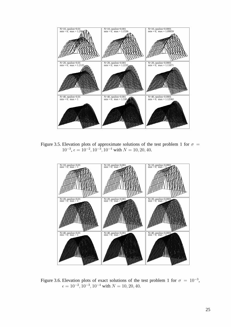
Figure 3.5. Elevation plots of approximate solutions of thetest problem 1 forσ =

10−3, ǫ = 10−2, 10−3, 10−4 with N = 10, 20, 40. . . . . . . . . . . . . . . . . . . . . . . . . .25

Figure 3.6. Elevation plots of exact solutions of the test problem 1 forσ = 10−3,

ǫ = 10−2, 10−3, 10−4 with N = 10, 20, 40. . . . . . . . . . . . . . . . . . . . . . . . . . . . . . . . .25

Figure 3.7. Contour plots of approximate solutions of the test problem 1 forσ =

10−3 ǫ = 10−2, 10−3, 10−4 with N = 10, 20, 40. . . . . . . . . . . . . . . . . . . . . . . . . . .26

Figure 3.8. Contour plots of exact solutions of the test problem 1 forσ = 10−3,

ǫ = 10−2, 10−3, 10−4 with N = 10, 20, 40. . . . . . . . . . . . . . . . . . . . . . . . . . . . . . . . .26

viii

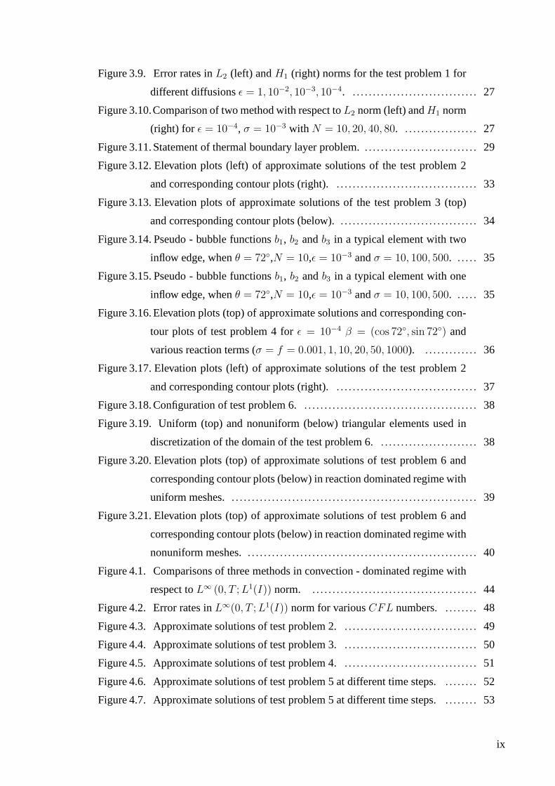
Figure 3.9. Error rates inL2 (left) andH1 (right) norms for the test problem 1 for

different diffusionsǫ = 1, 10−2, 10−3, 10−4. . . . . . . . . . . . . . . . . . . . . . . . . . . . . . . .27

Figure 3.10.Comparison of two method with respect toL2 norm (left) andH1 norm

(right) for ǫ = 10−4, σ = 10−3 with N = 10, 20, 40, 80. . . . . . . . . . . . . . . . . . . 27

Figure 3.11. Statement of thermal boundary layer problem.. . . . . . . . . . . . . . . . . . . . . . . . . . . .29

Figure 3.12. Elevation plots (left) of approximate solutions of the test problem 2

and corresponding contour plots (right).. . . . . . . . . . . . . . . . . . . . . . . . . . . . . . . . . . .33

Figure 3.13. Elevation plots of approximate solutions of the test problem 3 (top)

and corresponding contour plots (below).. . . . . . . . . . . . . . . . . . . . . . . . . . . . . . . . . .34

Figure 3.14. Pseudo - bubble functionsb1, b2 andb3 in a typical element with two

inflow edge, whenθ = 72,N = 10,ǫ = 10−3 andσ = 10, 100, 500. . . . . . 35

Figure 3.15. Pseudo - bubble functionsb1, b2 andb3 in a typical element with one

inflow edge, whenθ = 72,N = 10,ǫ = 10−3 andσ = 10, 100, 500. . . . . . 35

Figure 3.16. Elevation plots (top) of approximate solutions and corresponding con-

tour plots of test problem 4 forǫ = 10−4 β = (cos 72, sin 72) and

various reaction terms (σ = f = 0.001, 1, 10, 20, 50, 1000). . . . . . . . . . . . . . 36

Figure 3.17. Elevation plots (left) of approximate solutions of the test problem 2

and corresponding contour plots (right).. . . . . . . . . . . . . . . . . . . . . . . . . . . . . . . . . . .37

Figure 3.18. Configuration of test problem 6.. . . . . . . . . . . . . . . . . . . . . . . . . . . . . . . . . . . . . . . . . . .38

Figure 3.19. Uniform (top) and nonuniform (below) triangular elements used in

discretization of the domain of the test problem 6.. . . . . . . . . . . . . . . . . . . . . . . .38

Figure 3.20. Elevation plots (top) of approximate solutions of test problem 6 and

corresponding contour plots (below) in reaction dominatedregime with

uniform meshes.. . . . . . . . . . . . . . . . . . . . . . . . . . . . . . . . . . . . . . . . . . . . . . . . . . .. . . . . . . . . . 39

Figure 3.21. Elevation plots (top) of approximate solutions of test problem 6 and

corresponding contour plots (below) in reaction dominatedregime with

nonuniform meshes.. . . . . . . . . . . . . . . . . . . . . . . . . . . . . . . . . . . . . . . . . . . . . . . . . . .. . . . . . 40

Figure 4.1. Comparisons of three methods in convection - dominated regime with

respect toL∞ (0, T ;L1(I)) norm. . . . . . . . . . . . . . . . . . . . . . . . . . . . . . . . . . . . . . . . . .44

Figure 4.2. Error rates inL∞(0, T ;L1(I)) norm for variousCFL numbers. . . . . . . . . 48

Figure 4.3. Approximate solutions of test problem 2.. . . . . . . . . . . . . . . . . . . . . . . . . . . . . . . . .49



Figure 4.6. Approximate solutions of test problem 5 at different time steps. . . . . . . . . 52

Figure 4.7. Approximate solutions of test problem 5 at different time steps. . . . . . . . . 53

ix

LIST OF TABLES

Table Page

Table 2.1. Errors inL2 norm for various values ofh when the problem (2.1) is in

diffusion - dominated regime.. . . . . . . . . . . . . . . . . . . . . . . . . . . . . . . . . . . . . . . . . . . . . . .9

Table 2.2. Errors inH1 norm for various values ofh when the problem (2.1) is in

diffusion - dominated regime.. . . . . . . . . . . . . . . . . . . . . . . . . . . . . . . . . . . . . . . . . . . . . . .10

Table 2.3. Errors inL2 norm for various values ofh when the problem (2.1) is in

convection - dominated regime.. . . . . . . . . . . . . . . . . . . . . . . . . . . . . . . . . . . . . . . . . . . . .13

Table 2.4. Errors inH1 norm for varioush when the problem (2.1) is in convec-

tion - dominated regime.. . . . . . . . . . . . . . . . . . . . . . . . . . . . . . . . . . . . . . . . . . . . . . . . . . .. 13

Table 3.1. Errors of the test problem 1 inL2 norm for variousN with σ = 10−3

and different diffusionsǫ = 1, 10−2, 10−3, 10−4 . . . . . . . . . . . . . . . . . . . . . . . . . . .28

Table 3.2. Errors of the test problem 1 inH1 norm for variousN with σ = 10−3

and different diffusionsǫ = 1, 10−2, 10−3, 10−4. . . . . . . . . . . . . . . . . . . . . . . . . . .28

x

CHAPTER 1

INTRODUCTION

1.1. Introduction

Convection - diffusion - reaction (CDR) problem is one of themost frequently

used model problem in science and engineering. This model problem describes how the

concentration of a number of substances (e.g., pollutants,chemicals, electrons) distributed

in a medium changes under the influence of three processes, namely convection, diffusion

and reaction.Convectionrefers to the movement of a substance within a medium (e.g.,

water or air). Diffusion refers to the movement of the substance from an area of high

concentration to an area of low concentration, resulting inthe uniform distribution of the

substance. A chemicalreactionis a process that results in the inter-conversion of chemical

substance. Thus simulations of convection - diffusion - reaction equations are required in

various applications. Numerical simulations of convection - diffusion - reaction problems

have been studied actively during the last thirty five years.

A characteristic feature of solutions of convection - diffusion - reaction problems

is the presence of sharp layers. When convection or reactiondominates, there are physical

effects in the problem that occur on a scale which is much smaller than the smallest one

representable on the computational grid. However such effects have a strong impact on

the larger scale. It is known that plain Galerkin method produces undesired oscillations

that pollute whole domain in the presence of under-resolvedlayers.

Petrov-Galerkin method changing the shape of the test functions is one of the ear-

liest attempts to cure this situation. In order to gain the control of derivatives Streamline-

Upwind Petrov Galerkin (SUPG) method which is first proposedin (Brooks & Hughes

1982) is a much more general approach where the variational formulation is augmented.

The advantages of this method are its great generality to analyze and to derive the error

bounds. The main drawback of SUPG method is the presence of a stabilizing parameter

that needs to be properly chosen.

Another approach is Residual-Free-Bubble (RFB) method which is based on en-

riching the finite element space. It is first studied in (Baiocchi et al. 1993) to find a

suitable value of stabilizing parameter for SUPG method. The main problem with this

method is that it requires the solution of a local PDE. Cheap approximate solutions to this

1

local problem were designed by several researchers (Baiocchi et al. 1993), (Nesliturk

1999), (Brezzi et al. 1998), (Brezzi et al. 2003), ( Sendur &Nesliturk 2011). Link-

Cutting Bubble (LCB) strategy aims to stabilize the Galerkin method by using a suitable

refinement near the layer region. LCB strategy uses the piecewise linear bubble functions

to find the suitable sub-grid nodes. It works as the plain Galerkin method on augmented

meshes. It is extended to time-dependent convection - diffusion - reaction problem in one

dimension in (Asensio et al. 2007). One of the drawback of this strategy is that in limit

regimes sub-grid nodes are very close to the original nodes so undesired oscillations may

occur at sub-grid nodes near layers for unsteady problems. Hence, in numerical simula-

tions one has to exclude the sub-grid nodes. Another drawback of LCB strategy is that in

two dimensions it is very difficult to implement because of its technique.

Pseudo Residual-Free Bubble (P-RFB) method aims to get sub-grid nodes to ap-

proximate bubble functions cheaply using piecewise linearfunctions ( Sendur & Nes-

liturk 2011). The main advantage of P-RFB method is that it can be implemented in two

dimensions ( Sendur et al. 2012). Another advantage of thismethod is that since integrals

of P-RFB functions are directly used when constructing the mass matrix, a smaller mass

matrix is used with respect to the mass matrix constructed inLCB strategy.

In my thesis we will examine P-RFB method for both steady and unsteady con-

vection - diffusion - reaction problems in one and two space dimensions.

1.2. Layout of the Thesis

Chapter 2 reviews RFB method and P-RFB method in one dimension for steady

convection - diffusion - reaction problems. Comparisons are done between P-RFB method,

LCB strategy and SUPG method in different regimes. Approximate solutions and error

rates inL2 norm are given.

Chapter 3 deals with steady convection - diffusion - reaction problems in two

dimensions and examines P-RFB method in different regimes.A comparison is done

between P-RFB and SUPG methods. Approximate solutions in different regimes are

given.

Chapter 4 is devoted to extension of P-RFB method to unsteadyconvection - dif-

fusion - reactions problems. Variational formulations of P-RFB method, LCB strategy

and SUPG method are given in one dimension.CFL numbers at which P-RFB method,

LCB strategy and SUPG method work best with Crank-Nicolson scheme are determined.

Then comparisons between the methods at theseCFL numbers are done. Finally, the

2

thesis extends P-RFB method to unsteady convection - diffusion - reaction problems in

two dimensions. Variational formulations of P-RFB and SUPGmethods are given. A

comparison between these two methods with Bacward-Euler scheme is established.

3

CHAPTER 2

PSEUDO RESIDUAL - FREE BUBBLES FOR STEADY

CONVECTION - DIFFUSION - REACTION PROBLEMS IN

ONE DIMENSION

In this section, we will show a stabilization method for one -dimensional steady

convection - diffusion - reaction problems, designed to treat the most interesting case of

small diffusion, but able to adapt one regime to another continuously which is studied in

( Sendur & Nesliturk 2011). This method aims to approximate the RFB functions effi-

ciently but cheaply without compromising the accuracy. Thepseudo bubbles are chosen

to be piecewise linear on a suitable sub-grid that, the position of whose nodes are deter-

mined by minimizing the residual of local differential problems with respect toL1 norm

( Sendur & Nesliturk 2011). Location of sub-grid nodes in (Sendur & Nesliturk 2011)

coincides with the location of sub-grid nodes in (Brezzi et al. 2003) when the problem is

in reaction - dominated regime.

2.1. A Review of RFB Method in One Dimension

Consider the two point boundary value problem

Lu = −ǫu′′ + βu′ + σu = f(x) on I,

u(0) = u(1) = 0,(2.1)

whereI = (0, 1). Let Th = K be a decomposition ofI whereK = (xk−1, xk), k =

1, ..., N . For simplicity we shall assume that the subintervals are uniform so that length

of each subinterval ish. We also assume that diffusion coefficientǫ is positive constant

and convection fieldβ and reaction fieldσ are non-negative constants. It is well known

that when diffusion coefficientǫ is small with respect toβ orσ, Galerkin method produces

oscillations as depicted in Fig. 2.1. To treat this case several stabilized methods have been

introduced such as SUPG (Streamline - Upwind Petrov/Galerkin) method which is first

described in (Brooks & Hughes 1982) and the RFB method which is based on augmenting

the finite element space of linear basis functions. RFB method can be summarized as

4

0

0.2

0.4

0.6

0.8

1

1.2

0 0.2 0.4 0.6 0.8 1

Figure 2.1. Standard Galerkin finite element method withǫ = 0.001, β = 1, σ = 1andh = 0.02 subject to homogeneous boundary condition.

follows. Let start with recalling abstract variational formulation of problem (2.1): Find

u ∈ H10 (I) such that

a(u, v) = (f, v), ∀v ∈ H10 (I), (2.2)

where

a(u, v) = ǫ

∫

I

u′v′dx+

∫

I

(βu)′vdx+

∫

I

σuvdx. (2.3)

DefineVh subspace ofH10 (I) as finite - dimensional space. Then Galerkin finite element

method reads: Finduh ∈ Vh such that

a(uh, vh) = (f, vh), ∀vh ∈ Vh. (2.4)

Now, decompose the spaceVh asVh = VL⊕

VB, whereVL is the space of continuous

piecewise linear polynomials andVB =⊕

K BK with BK = H10 (K). From this decom-

position everyvh ∈ Vh can be written in the formvh = vL + vB, wherevL ∈ VL and

vB ∈ VB. Bubble componentuB of uh satisfy the original differential equation in an

element K strongly, i.e.

LuB = −LuL + f in K, (2.5)

5

subject to boundary condition,

uB = 0 on ∂K. (2.6)

Since the support of bubbleuB is contained within the elementK we can make a static

condensation for the bubble part, getting directly theVL- projectionuL of the solutionuh

(Brezzi & Russo 1993). This can be done as follows. UsingVh = VL⊕

VB, the finite

element approximation reads: Finduh = uL + uB in Vh such that

a(uL, vL) + a(uB, vL) = (f, vL), ∀vL ∈ VL. (2.7)

From equations (2.5) and (2.6),uB is identified by the linear partuL and source function

0

0.2

0.4

0.6

0.8

1

0 0.02 0.04 0.06 0.08 0.1

"RFB""P-RFB"

0

0.2

0.4

0.6

0.8

1

0 0.02 0.04 0.06 0.08 0.1

"RFB""P-RFB"

Figure 2.2. Comparison of exact solution (curved line) of the optimal bubble with itspiecewise linear approximation for problem parametersǫ = 0.005, β = 1,σ = 0.001 (left) andǫ = 0.0001, β = 1, σ = 0.001 (right).

f , which is as complicated as solving the original differential equation. Therefore, it is

important to bring a cheap approximation to the bubble function which gives a similar

stabilization effect as shown in Fig. 2.2 .

2.2. Pseudo - RFB in One Dimension

In order to make an efficient linear approximation to the bubbles, locations of

sub-grid nodes are crucial. This is accomplished by a minimization process with respect

6

to L1 norm in the presence of layers ( Sendur & Nesliturk 2011). Let z1 andz2 be two

sub-grid in a typical elementK = (xk−1, xk) such thatxk−1 < z1 < z2 < xk on which

we approximate the bubble functions. Assume thatf is a piecewise linear function with

respect to discretization. Then the residual in (2.5) becomes a linear function and it is

reasonable to consider bubble functionsBi (i = 1, 2) defined by

LBi = −Lϕi in K, Bi = 0 on∂K, i = 1, 2, (2.8)

whereϕ1, ϕ2 are the restrictions of the piecewise linear basis functions for VL to K.

Further defineBf such that

LBf = f in K, Bf = 0 on∂K. (2.9)

LetB∗i (x) = αibi(x) be the classical Galerkin approximation ofBi through (2.8), that is

a(B∗i , bi)K = (−Lϕi, bi)K , i = 1, 2, (2.10)

wherebi is a piecewise linear function with

bi(xk−1) = bi(xk) = 0, bi(zi) = 1, i = 1, 2. (2.11)

Using numerical integration and properties of bubble functions one can get explicit ex-

pressions ofα1 andα2 as follows:

α1 =3β + (ξ − 2h)σ

2h( 3ǫξ(h−ξ)

+ σ), α2 = −3β + (2h− η)σ

2h( 3ǫη(h−η)

+ σ), (2.12)

whereξ = z1−xk−1, η = xk−z2, δ = z2−z1. Now it remains to choosezi. The main idea

behind determining the locations of sub-grid nodes is to minimize residual with respect

toL1 norm coming out from equation (2.8). That is, choosezi such that

Ji =

∫

K

|LB∗i + Lϕi|dx, i = 1, 2, (2.13)

is minimum ( Sendur & Nesliturk 2011).

7

2.2.1. Diffusion - Dominated Regime

The problem is assumed to be diffusion - dominated when6ǫ > βh2/9 ( Sendur

& Nesliturk 2011). In this regime, stabilization is not needed and a uniform sub-grid is

chosen asξ = η = δ = h/3 ( Sendur & Nesliturk 2011).

2.2.2. Convection - Dominated Regime

The problem is convection - dominated if6ǫ < βh2/9 with 3β ≥ σh. The follow-

ing lemma which is given in ( Sendur & Nesliturk 2011) suggests an optimal position for

z2.

Lemma 1 In convection - dominated case, the pointηe =−3β+

√9β2+24ǫσ

2σminimizes the

integral (2.13) fori = 2.

There are several possibilities forξ in convection - dominated regime. To determine the

optimalξ, we look at the errors inL2 norm for various values ofξ. We set the diffusion

coefficientǫ = 10−5, the convective field toβ = 1 and reaction term toσ = 1 with exter-

nal sourcef = 1. From Fig. 2.3 we can see that optimalξ is h− η and error inL2 norm

is of order 2. Thus in convection - dominated regime we takeη = ηe andξ = h− η.

2.2.3. Reaction - Dominated Regime

In reaction - dominated regime position ofz2 is as in convection - dominated

regime. Note that the problem is in reaction - dominated regime if 6ǫ ≤ βh2/9 with

3β < σh. After the minimization of the integralJ1, ξ, η andδ are suggested as follows in

( Sendur & Nesliturk 2011):

ξe =3β +

√

9β2 + 24ǫσ

2σ, η = ηe, ξ = minh− η, ξe, δ = (h− η − ξ).

(2.14)

2.3. Numerical Experiments

In this section, we report some numerical experiments to illustrate the performance

of P-RFB ( Sendur & Nesliturk 2011), Link - Cutting Bubble Strategy (Brezzi et al. 2003)

8

10−3

10−2

10−1

10−6

10−5

10−4

10−3

10−2

h

||u−

u h|| L 2

h − eta

h − 1.2*eta

h − 1.4*eta

h − 2*eta

h − 0.9*eta

h − 0.5*eta

h − 0.1*eta

Figure 2.3. Optimalξ in convection - dominated regime.

and SUPG method. Stabilization parameterτ = 1/(2σ + 2βh+ 12ǫ

h2 ) for SUPG method is

taken from (Asensio et al. 2007). In this chapter all tests are done in the unit interval

(0.1) and uniform meshes are used.

2.3.1. Test 1 (Diffusion - Dominated Regime)

We start with the advection - diffusion - reaction problem (2.1) subject to ho-

mogeneous Dirichlet boundary condition when the problem isdiffusion dominated. The

diffusion coefficient is set toǫ = 1. The convective field is set toβ = 1 and the reaction

term toσ = 1 with external forcef = 1. Table 2.1. and Table 2.2. show the values of

errors inL2 andH1 norms forh = 0.05, 0.025, 0.0125, 0.00625, respectively. Fig 2.4.

Table 2.1. Errors inL2 norm for various values ofh when the problem (2.1) is indiffusion - dominated regime.

h=0.05 h=0.025 h=0.0125 h=0.00625P-RFB 0.00018 0.000046 0.000011 0.0000029LCB 0.00019 0.000047 0.000011 0.0000030

SUPG 0.00018 0.000045 0.000011 0.0000028

shows the error rates inL2 andH1 norms. In diffusion dominated regime all the three

9

Table 2.2. Errors inH1 norm for various values ofh when the problem (2.1) is indiffusion - dominated regime.

h=0.05 h=0.025 h=0.0125 h=0.00625P-RFB 0.012 0.0061 0.0030 0.0015LCB 0.012 0.0061 0.0030 0.0015

SUPG 0.012 0.0061 0.0030 0.0015

10−3

10−2

10−1

10−6

10−5

10−4

10−3

h

||u−

u h|| L 2

P−RFB

LCB

SUPG

10−3

10−2

10−1

10−3

10−2

10−1

h

||u−

u h|| H1

P−RFB

LCB

SUPG

Figure 2.4. Error rates inL2 andH1 norms when the problem (2.1) is in diffusion -dominated regime.

methods turn into Standard Galerkin finite element method and they give approximately

the same results.

2.3.2. Test 2 (Convection - Dominated Regime)

Our second numerical experiment is a test problem taken from(Brezzi et al.

2003) which is an advection - diffusion - reaction problem (2.1) subject to homoge-

nous Dirichlet boundary condition when the convection termis dominated. 11 nodes

are used for numerical approximations. The diffusion coefficient is set toǫ = 0.00001,

convection term toβ = 1 and reaction term is set toσ = 1. We assume external force

f = 1. Fig 2.5 shows the numerical approximations. Errors inL2 andH1 norms are

reported in Table 2.3. and Table 2.4. respectively. Fig. 2.6shows the error rates for

10

h = 0.05, 0.025, 0.0125, 0.00625. In convection - dominated regime error inL2 norm is

of order2 and inH1 norm is of order1 for the three methods. SUPG method produces an

oscillation near boundary layer.

2.3.3. Test 3 (Reaction - Dominated Regime)

We now consider the advection - diffusion - reaction problem(2.1) subject to ho-

mogenous Dirichlet boundary condition when reaction term is dominated. The diffusion

coefficient is set toǫ = 0.00001, convective field toβ = 1 and reaction term is set to

σ = 100. We assumef = 100. For numerical approximations (Fig. 2.7)21 nodes

are used. All the methods works fine in reaction dominated regime but SUPG method

produces oscillations again near boundary layers.

2.3.4. Test 4 (Internal Layer Problem)

Our last experiment is as in previous one advection - diffusion - reaction problem

(2.1) subject to Dirichlet boundary condition when reaction term is dominated but an

internal layer exists. The diffusion coefficient is set toǫ = 0.00001, convection term

to β = 1 and reaction term is set toσ = 50. External forcef is piecewise defined

such thatf = −50 for x ≤ 0.5 andf = 50 for x > 0.5. 41 nodes are used for numerical

approximations. From Fig 2.8 we can say that Pseudo - RFB is able to capture the internal

layer more accurately than the other ones. SUPG method produces oscillations near both

internal layer and boundary layer.

11

0

0.1

0.2

0.3

0.4

0.5

0.6

0.7

0 0.2 0.4 0.6 0.8 1

"P-RFB""exact"

0

0.1

0.2

0.3

0.4

0.5

0.6

0.7

0 0.2 0.4 0.6 0.8 1

"LCB""exact"

0

0.1

0.2

0.3

0.4

0.5

0.6

0.7

0 0.2 0.4 0.6 0.8 1

"SUPG""exact"

Figure 2.5. Approximate solutions when the problem (2.1) isin convection dominatedregime.

10−3

10−2

10−1

10−6

10−5

10−4

10−3

h

||u−

u h|| L 2

P−RFB

LCB

SUPG

10−2

10−1

10−3

10−2

h

||u−

u h|| H1

P−RFB

LCB

SUPG

Figure 2.6. Error rates inL2 andH1 norms when the problem (2.1) is in convection -dominated regime.

12

Table 2.3. Errors inL2 norm for various values ofh when the problem (2.1) is inconvection - dominated regime.

h=0.05 h=0.025 h=0.0125 h=0.00625P-RFB 0.00014 0.000036 0.0000092 0.0000023LCB 0.00014 0.000036 0.0000092 0.0000023

SUPG 0.00014 0.000036 0.0000091 0.0000022

Table 2.4. Errors inH1 norm for varioush when the problem (2.1) is in convection -dominated regime.

h=0.05 h=0.025 h=0.0125 h=0.00625P-RFB 0.0093 0.0046 0.0023 0.0011LCB 0.0093 0.0046 0.0023 0.0011

SUPG 0.0093 0.0046 0.0023 0.0011

0

0.2

0.4

0.6

0.8

1

1.2

0 0.2 0.4 0.6 0.8 1

"P-RFB""exact"

0

0.2

0.4

0.6

0.8

1

1.2

0 0.2 0.4 0.6 0.8 1

"LCB""exact"

0

0.2

0.4

0.6

0.8

1

1.2

0 0.2 0.4 0.6 0.8 1

"SUPG""exact"

Figure 2.7. Numerical approximations when the problem (2.1) is in reaction domi-nated regime.

13

-1.5

-1

-0.5

0

0.5

1

1.5

0 0.2 0.4 0.6 0.8 1

"P-RFB"

-1.5

-1

-0.5

0

0.5

1

1.5

0 0.2 0.4 0.6 0.8 1

"LCB"

-1.5

-1

-0.5

0

0.5

1

1.5

0 0.2 0.4 0.6 0.8 1

"SUPG"

Figure 2.8. Numerical approximations with an internal layer when the problem (2.1)is in reaction dominated regime.

14

CHAPTER 3

PSEUDO RESIDUAL - FREE BUBBLES FOR

CONVECTION - DIFFUSION - REACTION PROBLEMS IN

TWO DIMENSIONS

This section is devoted to the application of the Pseudo Residual - free Bubble

functions for the stabilization of two - dimensional steadyconvection - diffusion - reac-

tion problems. In one dimension two sub-grid nodes are sufficient. But in two dimensions

three sub-grid nodes are necessary in each triangular element to approximate the bubble

functions. Presence of three sub-grid nodes in an element makes LCB strategy very diffi-

cult to apply in two dimensions. However, since only integrals of Pseudo Residual - free

bubble functions are directly used in calculations withoutmodifying the given mesh, it

is easier to implement P-RFB method in two dimensions when the positions of sub-grid

nodes are in hand. Positions of these three sub-grid nodes are determined by minimizing

the residual of local differential problems with respect toL1 norm as in one dimension

( Sendur et al. 2012).

3.1. A Review of RFB Method in Two Dimensions

Consider the elliptic convection - diffusion - reaction problem on polygonal do-

mainΩ in 2D

Lu = −ǫ∆u + β.∇u+ σu = f on Ω,

u = 0 on ∂Ω,(3.1)

where the diffusion coefficientǫ is positive constant, convection termβ and reaction term

σ are non-negative constants. LetTh be a decomposition of the domainΩ in to triangles

K, and lethk = diam(K) with h = maxK∈Thhk. We assume thatTh is admissible (non

- overlapping triangles, their union reproduces the domain) and shape regular (the trian-

gles verify a minimum angle condition). We start by considering the abstract variational

15

formulation of the problem (3.1): Findu ∈ H10 (Ω) such that

a(u, v) = (f, v) ∀v ∈ H10 (Ω) (3.2)

wherea(u, v) = ǫ∫

Ω∇u.∇v +

∫

Ω(β.∇u)v +

∫

Ωσuv and(f, v) =

∫

Ωfv. DefineVh as

a finite dimensional subspace ofH10 (Ω). Then standard Galerkin finite element method

reads: Finduh ∈ Vh such that

a(uh, vh) = (f, vh) ∀vh ∈ Vh. (3.3)

We now decompose the spaceVh such thatVh = VL⊕

VB, whereVL is the space of

continuous piecewise linear polynomials andVB =⊕

K BK with BK = H10 (K). Then

vh = vL + vB can be uniquely written wherevL ∈ VL andvB ∈ VB. From the decom-

position ofVh into VL andVB, we require the bubble componentuB of uh to satisfy the

original differential equation inK strongly i.e.,

LuB = −LuL + f in K (3.4)

subject to boundary conditions,

uB = 0 on∂K. (3.5)

By the static condensation procedure, (Brezzi & Russo 1993)the method reads: Find

uh = uL + uB in Vh such that

a(uL, vL) + a(uB, vL) = (f, vL) ∀vL ∈ VL. (3.6)

The bubble component should be computed to solve (3.6). Fromequations (3.4) and (3.5)

bubble functionub is identified by the linear partuL and the source functionf which is as

complicated as solving the original differential equation. So it is important to get a cheap

approximation for the RFB functions which gives a similar stabilization effect ( Sendur

et al. 2012).

16

3.2. Pseudo RFB in Two Dimensions

In order to make an efficient linear approximation to the bubble functions, loca-

tions of sub-grid nodes are crucial. LetPi (i = 1, 2, 3) be these sub-grid nodes. Location

of those sub-grid nodes are determined by a minimization process with respect toL1 norm

in the presence of layers ( Sendur et al. 2012). Assume thatf is a piecewise linear func-

tion with respect to discretization. Then the residual in (3.4) becomes a linear function

and it is reasonable to consider bubble functionsBi (i = 1, 2) defined by

LBi = −Lϕi in K, Bi = 0 on∂K, i = 1, 2, 3 (3.7)

whereϕ1, ϕ2 andϕ3 are the restrictions of the piecewise linear basis functions for VL to

K. Further defineBf such that

LBf = f in K, Bf = 0 on∂K. (3.8)

Since

uL|K =3∑

i=1

ciϕi (3.9)

we can write

uB|K =3∑

i=1

ciBi +Bf (3.10)

with the same coefficientci. From here

LuB = −LuL + f in K. (3.11)

That is, equation (3.4) is automatically satisfied ( Senduret al. 2012). LetB∗i (x) =

αibi(x) be the classical Galerkin approximation ofBi through (3.7) that is,

a(B∗i , bi)K = (−Lϕi, bi)K , i = 1, 2 (3.12)

17

wherebi is a piecewise linear function such that

bi(Vj) = 0 and bi(Pi) = 1 ∀i, j = 1, 2, 3 (3.13)

whereVi are the vertices ofK. From equation (3.12) one can easily get

αi =−(Lϕi, bi)

a(bi, bi)=

−(Lϕi, bi)

ǫ||∇bi||2K + σ||bi||2Ki = 1, 2, 3 (3.14)

where in equation (3.14) the following fact is used ( Senduret al. 2012);

∫

K

(β.∇bi)bi =∫

K

∇.(βbi)bi−∫

K

(∇.β)bibi =∫

∂K

(βbibi).da−∫

K

0 ∗ bibi = 0+0 = 0.

(3.15)

To determine the location of internal points,L1 minimization process is applied to the

following integral coming out from the bubble equation (3.7) ( Sendur et al. 2012)

Ji =

∫

K

|LB∗i + Lϕi|, i = 1, 2, 3. (3.16)

Before giving the explicit expression of internal nodes fordifferent regimes, we will give

additional notation about element geometry. Edges ofK are denoted byei opposite toVi,

length ofei by |ei|, the midpoint of edgeei by Mi, the outward unit normal toei by ni,

νi = |ei|ni andβνi = (β, νi). If βν1 < 0, βν2 > 0 andβν3 > 0 then the element has only

one inflow edge and ifβν1 > 0, βν2 < 0 andβν3 < 0 then the element has two inflow

edges as depicted in Fig 3.1.

3.2.1. Diffusion - Dominated Regime

Location ofPi along the median fromVi is defined as

Pi = (1− ti)Mi + tiVi, 0 < ti < 1, i = 1, 2, 3. (3.17)

t1, t2, andt3 are defined for both one inflow and two inflow edge ast1 = t2 = t3 = 1/3

( Sendur et al. 2012). That is when the problem is in diffusion dominated regime the

sub-grid nodes are at the barycentre of triangular element.

18

Figure 3.1. Configuration of internal nodes for element has one inflow edge (left) andtwo inflow edge (right).

3.2.2. Convection - Dominated Regime

We consider the both one inflow edge element and two inflow edges element and

we start with one inflow edge.

3.2.2.1. One Inflow Edge

Location ofPi along the median fromVi is defined as

Pi = (1− ti)Mi + tiVi, 0 < ti < 1, i = 1, 2, 3. (3.18)

The problem is in convection - dominated regime ifǫ ≤ ǫ∗1 with 2σ|K| < minβν2 , βν3where

ǫ∗1 =2|K|(−3βν1 + σ|K|)9(|e1|2 + |e2|2 + |e3|2)

. (3.19)

The following lemma which is given in ( Sendur et al. 2012) suggests an optimal position

for P1 along the median fromV1.

Lemma 1 If the inflow boundary make up of one edge, then the pointt∗1 = 1−−ρ1+√

ρ21+λ1

2σ|K|2

minimizes the integral (3.16) fori = 1 in convection - dominated flows whereρ1 =

19

Figure 3.2. Pseudo - bubble functionsb1, b2 andb3 in a typical element with one inflowedge, whenθ = 72,N = 20,ǫ = 10−2, 10−3, 10−4.

−2βν1 |K|+ 3ǫ|e2 − e3|2 andλ1 = 24ǫσ|K|2(|e2|2 + |e3|2).The choice of other two pointsP2 andP3 should be consistent with the physics of the

problem. Thus in convection dominated regime we take

t1 = t∗1 if ǫ < ǫ∗1,

t1 = 1/3 otherwise,

t2 = t3 = min1/3, 1− t∗1.(3.20)

In Fig 3.2 the behaviours of approximate bubble functions ina typical elementK with one

inflow edge, forβ = (cos 72, sin 72), σ = 0.001 and variousǫ are displayed. The first

column of the figure represents the bubble functionb1 for decreasing values of diffusion

(ǫ = 10−2, 10−3, 10−4). The corresponding numerical results forb2 andb3 are shown in

columns2 and3 respectively.

20

3.2.2.2. Two Inflow Edges

Now let the inflow boundary make up of two edges and lete2 ande3 be the inflow

ones. The problem is convection dominated ifǫ ≤ minǫ∗1, ǫ∗2 where

ǫ∗i =2|K|(−3βνi + σ|K|)9(|e1|2 + |e2|2 + |e3|2)

i = 1, 2. (3.21)

The following lemmas suggest optimal positions forP2 andP3. Proof of the lemmas are

given in ( Sendur et al. 2012).

Lemma 2 If the inflow boundary make up of two edges, then the pointt∗2 = 1 −−ρ2+

√ρ22+λ2

2σ|K|2minimizes the integral (3.16) fori = 2 in convection - dominated flows

whereρ2 = −2βν2 |K|+ 3ǫ|e1 − e3|2 andλ2 = 24ǫσ|K|2(|e1|2 + |e3|2).Lemma 3 If the inflow boundary make up of two edges, then the pointt∗3 = 1 −−ρ3+

√ρ23+λ3

2σ|K|2minimizes the integral (3.16) fori = 3 in convection - dominated flows

whereρ3 = −2βν3 |K|+ 3ǫ|e1 − e2|2 andλ3 = 24ǫσ|K|2(|e1|2 + |e2|2).For convection dominated regime, the choice of other pointP1 should be consistent with

the physics of the problem. Thus we take

t2 = t∗2, t3 = t∗3, t1 = min1/3, 1− t∗2, 1− t∗3. (3.22)

In Fig 3.3 the behaviours of pseudo - bubble functions in a typical elementK with two

inflow edge, forβ = (cos 72, sin 72), σ = 0.001 and variousǫ are displayed. The first

column of the figure represents the bubble functionb1 for decreasing values of diffusion

(ǫ = 10−2, 10−3, 10−4). The corresponding numerical results forb2 andb3 are shown in

columns2 and3 respectively.

3.2.2.3. Numerical Tests

In this section, we present some numerical experiments to assess the accuracy and

performance of P-RFB method. We shall report errors inL2 andH1 norms and a com-

parison is done between SUPG and P-RFB methods in terms ofL2 andH1 norms. In

our calculations we take different partitions of domainΩ. N represents the number of

element in eachx andy direction for uniformly partitioned domains.

21

Figure 3.3. Pseudo - bubble functionsb1, b2 andb3 in a typical element with two inflowedge, whenθ = 72,N = 20,ǫ = 10−2, 10−3, 10−4.

Test 1(Convection - dominated regime)

We start with considering the advection - diffusion - reaction equation (3.1) on a

unit square that can be solved analytically. We consider following problem

−ǫ∆u + (1, 0).∇u+ σu = 0, (3.23)

subject to boundary conditions (see Fig 3.4)

u =

0, if y = 0, 0 ≤ x ≤ 1,

0, if x = 1, 0 ≤ y ≤ 1,

0, if y = 1, 0 ≤ x ≤ 1,

sin(πy), if x = 0, 0 ≤ y ≤ 1.

(3.24)

Analytical solution of test problem 1:

Let u(x, y) = h(x)g(y) be our solution. Substitutingu(x, y) into the equation (3.23)

22

Figure 3.4. Configuration of test problem 1.

we get

−ǫh′′g − ǫg′′ + h′g + σhg = 0. (3.25)

Seperating the variables in equation (3.25)

−ǫh′′

h+h′

h+ σ = ǫ

g′′

g= −λ (3.26)

whereλ is a constant. From equation (3.26) and the given boundary conditions

ǫg′′ + λg = 0, g(0) = 0, g(1) = 0 (3.27)

ǫh′′ − h′ − h(λ+ σ), h(1) = 0. (3.28)

Equation (3.27) is a two point boundary value problem and itssolution is of the form

g(y) = c1 sin(

√

λnǫy) (3.29)

whereλn = ǫn2π2, n = 1, 2, 3, ... andc1 is a constant. Solution of equation (3.28) is of

23

the form

h(x) = ex

2ǫ

(

c2 sinh

(

√

1 + 4ǫ(σ + ǫn2π2)

2ǫ(x− 1)

))

(3.30)

wherec2 is a constant. From superposition principle

u(x, y) =∞∑

n=1

Anex

2ǫ sinh

(

√

1 + 4ǫ(σ + ǫn2π2)

2ǫ(x− 1)

)

sin(nπy). (3.31)

Using orthogonality ofsin function and last boundary condition

A1 =1

sinh

(

−√

1+4ǫ(σ+ǫπ2)

2ǫ

) , An = 0 for n = 2, 3, .... (3.32)

Hence our solution is

u(x, y) = ex

2ǫ

1

sinh

(

−√

1+4ǫ(σ+ǫπ2)

2ǫ

) sinh

(

√

1 + 4ǫ(σ + ǫπ2)

2ǫ(x− 1)

)

sin(πy).

(3.33)

Elevation plots of approximate and exact solutions forσ = 10−3 and for different dif-

fusions (ǫ = 10−2, 10−3, 10−4) with N = 10, 20, 40 are represented respectively in Fig

3.5 and Fig 3.6. The columns represent the solutions with a certain ǫ and increasingN .

Corresponding contour plots are represented in Fig 3.7 and Fig 3.8 respectively. In Table

3.1 and Table 3.2 errors inL2 andH1 norms are reported respectively. In Fig 3.9 error

rates are represented inL2 andH1 norms respectively. It can be seen from numerical

calculations that the error inL2 norm is of order2 and inH1 norm is of order1 which are

the expected orders. The method works fine in limit regimes. In Fig 3.10 a comparison

between SUPG and P-RFB method is represented with respect toL2 andH1 norm. Sta-

bilization parameter for SUPG methodτ = 1/( 4ǫh2

k

+ 2|β|hk

+ σ) wherehk is an appropriate

measure for the size of the mesh cell, is taken from (Codina 1998). SUPG and P-RFB

methods approximately have the same quality in convection dominated regime.

Test 2(Thermal boundary layer problem)

Now we consider a problem taken from (Nesliturk 1999). Let us consider a

24

N=10, epsilon=0.01min = 0, max = 1.298

N=10, epsilon=0.001min = 0, max = 1.1536

N=10, epsilon=0.0001min = 0, max = 1.09959

N=20, epsilon=0.01min = 0, max = 1.2125

N=20, epsilon=0.001min = 0, max = 1.2235

N=20, epsilon=0.0001min = 0, max = 1.11071

N=40, epsilon=0.01min = 0, max = 1

N=40, epsilon=0.001min = 0, max = 1.330

N=40, epsilon=0.0001min = 0, max = 1.12582

Figure 3.5. Elevation plots of approximate solutions of thetest problem 1 forσ =10−3, ǫ = 10−2, 10−3, 10−4 with N = 10, 20, 40.



N=10, epsilon=0.0001min = 0, max = 1



N=20, epsilon=0.0001min = 0, max = 1



N=40, epsilon=0.0001min = 0, max = 1

Figure 3.6. Elevation plots of exact solutions of the test problem 1 forσ = 10−3,ǫ = 10−2, 10−3, 10−4 with N = 10, 20, 40.

25

N=10, epsilon=0.01

min = 0, max = 1.29804

N=10, epsilon=0.001

min = 0, max = 1.1536

N=10, epsilon=0.0001

min = 0, max = 1.09959

N=20, epsilon=0.01

min = 0, max = 1.21259

N=20, epsilon=0.001

min = 0, max = 1.2235


min = 0, max = 1.11071

N=40, epsilon=0.01

min = 0, max = 1

N=40, epsilon=0.001

min = 0, max = 1.33056


min = 0, max = 1.12582

Figure 3.7. Contour plots of approximate solutions of the test problem 1 forσ = 10−3

ǫ = 10−2, 10−3, 10−4 with N = 10, 20, 40.

N=10, epsilon=0.01

min = 0, max = 1

N=10, epsilon=0.001

min = 0, max = 1


min = 0, max = 1

N=20, epsilon=0.01

min = 0, max = 1

N=20, epsilon=0.001

min = 0, max = 1


min = 0, max = 1

N=40, epsilon=0.01

min = 0, max = 1

N=40, epsilon=0.001

min = 0, max = 1


min = 0, max = 1

Figure 3.8. Contour plots of exact solutions of the test problem 1 forσ = 10−3, ǫ =10−2, 10−3, 10−4 with N = 10, 20, 40.

26

10−1

10−5

10−4

10−3

10−2

10−1

h

||u−

u h|| L 2

epsilon:1

epsilon:0.01

epsilon:0.001

epsilon:0.0001

10−1

10−2

10−1

100

h

||u−

u h|| H1

epsilon:1

epsilon:0.01

epsilon:0.001

epsilon:0.0001

Figure 3.9. Error rates inL2 (left) andH1 (right) norms for the test problem 1 fordifferent diffusionsǫ = 1, 10−2, 10−3, 10−4.

10−1

10−5

10−4

10−3

10−2

10−1

h

||u−

u h|| L 2

P−RFBSUPG

10−1

10−2

10−1

100

h

||u−

u h|| H1

P−RFBSUPG

Figure 3.10. Comparison of two method with respect toL2 norm (left) andH1 norm(right) for ǫ = 10−4, σ = 10−3 with N = 10, 20, 40, 80.

27

Table 3.1. Errors of the test problem 1 inL2 norm for variousN with σ = 10−3 anddifferent diffusionsǫ = 1, 10−2, 10−3, 10−4

N=10 N=20 N=40 N=80ǫ=1 0.003202 0.000804 0.000200 0.0000501ǫ=0.01 0.0486 0.00905 0.000369 0.0000899ǫ=0.001 0.0201 0.00489 0.000903 0.000113ǫ=0.0001 0.0131 0.00193 0.000314 0.0000587

Table 3.2. Errors of the test problem 1 inH1 norm for variousN with σ = 10−3 anddifferent diffusionsǫ = 1, 10−2, 10−3, 10−4.

N=10 N=20 N=40 N=80ǫ=1 0.105 0.0530 0.0263 0.01288ǫ=0.01 0.832 0.273 0.0263 0.0129ǫ=0.001 0.285 0.140 0.0585 0.0156ǫ=0.0001 0.19 0.0611 0.0275 0.0137

rectangular domain of sides1.0 and0.5, subject to following boundary conditions

u =

1, if x = 0, 0 ≤ y ≤ 0.5,

1, if y = 0.5, 0 ≤ x ≤ 1,

0, if y = 0, 0 ≤ x ≤ 1,

2y, if x = 1, 0 ≤ y ≤ 0.5.

(3.34)

The flow is taken asβ = (2y, 0) (see Fig 3.11). In each element we consider the vari-

able component of flow as constant i.e. we take the average value of2y at nodes in each

element. This problem may be viewed as the simulation of the development of a thermal

boundary layer on a fully developed flow between two parallelplates, where the top plate

is moving with velocity equal to one and the bottom plate is fixed. In our test we take

the diffusionǫ = 10−5 and the reaction termσ = 10−3. In Fig 3.12 the elevation plots of

approximate solutions and corresponding contour plots arepresented forN = 10, 20, 40.

Test 3(Propagation of discontinuity on boundary through the wind)

28

Figure 3.11. Statement of thermal boundary layer problem.

Our last problem for convection - dominated regime is about propagation of dis-

continuity on boundary. We use a uniform triangulations on unit square. We take diffu-

sionsǫ = 10−2, 10−3, convective fieldβ = (cos 72, sin 72) and reaction termσ = 10−3

with N = 20, 40, 80. In Fig 3.13 elevation plots of approximate solutions and their cor-

responding contour plots are presented. The first column of the figure represents the

approximate solutions and their corresponding contour plots for decreasing diffusions

(ǫ = 10−2, 10−3).

3.2.3. Reaction - Dominated Regime

Again we consider both one inflow edge element and two inflow edges element.

We start with considering the two inflow edges element.

3.2.3.1. Two Inflow Edges

The problem is reaction - dominated ifǫ ≤ minǫ∗2, ǫ∗3 with σ|K| > 3βν1

( Sendur et al. 2012). Position ofP2 andP3 are as in convection - dominated regime. It

remains to define location ofP1. Location ofPi along the median fromVi is defined as

Pi = (1− ti)Mi + tiVi, 0 < ti < 1, i = 1, 2, 3. (3.35)

The following lemma suggests optimal position forP1. Proof of the lemma is given in

( Sendur et al. 2012).

Lemma 4 If the inflow boundary make up of two edges, then the pointt∗∗1 = 1 −

29

ρ1+√

ρ21+λ1

2σ|K|2minimizes the integral (3.16) fori = 1 in reaction - dominated flows where

ρ1 = 2βν1|K| − 3ǫ|e2 − e3|2 andλ1 = 24ǫσ|K|2(|e2|2 + |e3|2).Thus we taket1, t2 andt3 as follows ( Sendur et al. 2012) :

t2 = t∗2,

t3 = t∗3,

t1 = maxmin1/3, 1− t2, 1− t3, t∗∗1 .(3.36)

In Fig 3.14 the behaviours of pseudo - bubble functions in a typical elementK with two

inflow edges, forβ = (cos 72, sin 72), ǫ = 10−3 and variousσ are displayed. The first

column of the figure represents the bubble functionb1 for increasing values of reaction

(σ = 10, 100, 500). The corresponding numerical results forb2 and b3 are shown in

column2 and3 respectively.

3.2.3.2. One Inflow Edge

In this case, the problem is reaction - dominated if ( Senduret al. 2012)

ǫ ≤ ǫ∗1 with σ|K| > 3maxβν2 , βν3. (3.37)

Position ofP1 is as in convection - dominated regime. It remains to define locations of

P2 andP3. The following lemmas suggests optimal positions forP2 andP3. Proofs of the

lemmas are given in ( Sendur et al. 2012).

Lemma 5 If the inflow boundary make up of one edge, then the pointt∗∗2 = 1− ρ2+√

ρ22+λ2

2σ|K|2

minimizes the integral (3.16) fori = 2 in reaction-dominated flows whereρ2 = 2βν2 |K|−3ǫ|e1 − e3|2 andλ2 = 24ǫσ|K|2(|e1|2 + |e3|2).Lemma 6 If the inflow boundary make up of one edge, then the pointt∗∗3 = 1− ρ3+

√ρ23+λ3

2σ|K|2

minimizes the integral (3.16) fori = 3 in reaction - dominated flows whereρ3 = 2βν3|K|−3ǫ|e1 − e2|2 andλ3 = 24ǫσ|K|2(|e1|2 + |e2|2).Thus we taket1, t2 andt3 as follows ( Sendur et al. 2012) :

t1 = t∗1,

t2 = max1− t1, t∗∗2 ,

t3 = max1− t1, t∗∗3 .

(3.38)

30

In Fig 3.15 the behaviours of pseudo - bubble functions in a typical elementK with

one inflow edge, forθ = 72, ǫ = 10−3 and variousσ are displayed. The first column

of the figure represents the bubble functionb1 for increasing values of reaction(σ =

10, 100, 500). The corresponding numerical results forb2 andb3 are shown in column2

and3 respectively.

3.2.3.3. Numerical Tests

Now we presents three numerical experiments to asses the quality of P-RFB method

in reaction dominated regime. Our first and second test show continuous transition of sub-

grid nodes from one regime to another. Third test is done whenthe problem is reaction

dominated without external source.

Test 4(Continuous transition from one regime to another)

This test problem is convection - diffusion - reaction problem (3.1) taken from

(Asensio et al. 2004). We takeǫ = 10−4, β = (cos 72, sin 72) with various reaction

terms (σ = f = 0.001, 1, 10, 20, 50, 1000) with N = 20. Elevation plots of approximate

solutions and their corresponding contour plots are presented in Fig 3.16. From Fig 3.16

we can say that P-RFB method has continuous transition between convection - dominated

regime and reaction - dominated regime.

Test 5(Continuous transition from one regime to another)

Now, we consider convection - diffusion - reaction problem (3.1) with ǫ = 10−3,

f = 1 andβ = (cos 72, sin 72) with homogenous Dirichlet boundary conditions. In

Fig 3.17 elevation plots of approximate solutions for the given data are presented with in-

creasing reaction from left to right and from top to bottom. From Fig 3.17 we can say that

P-RFB method satisfies continuous transition between convection - dominated regime and

reaction dominated regime for this problem.

Test 6(Reaction - dominated regime)

Our last test problem is taken from (Franca & Valentin 2000).Problem con-

figurations are displayed in Fig 3.18. In this problem we testour method with uniform

31

and nonuniform meshes (see Fig 3.19). Our discretizations consist of200 and400 el-

ements. We takeǫ = 10−4, β = (0.15, 0.1) andf = 0 for various values of reaction

(σ = 10, 102, 103). In Fig 3.20 and Fig 3.21 elevation plots of approximate solutions and

corresponding contour plots for uniform and nonuniform discretizations are presented

respectively. As we see from Fig 3.20 and Fig. 3.21 when the problem is in reaction

dominated regime, P-RFB method works perfect.

32

N=10, min = 0, max = 1.042 N=10

min = 0, max = 1.042

N=20, min = 0, max = 1.077 N=20

min = 0, max = 1.077

N=40, min = 0, max = 1.14281 N=40

min = 0, max = 1.14281

Figure 3.12. Elevation plots (left) of approximate solutions of the test problem 2 andcorresponding contour plots (right).

33

epsilon=0.01, N=20min = -0.002, max = 1.32

epsilon=0.01, N=40min = -0.00024, max = 1.059

epsilon=0.01, N=80min = 0, max = 1

epsilon=0.001, N=20min = -0.05, max = 1.40

epsilon=0.001, N=40min = -0.024, max = 1.389

epsilon=0.001, N=80min = -0.0093, max = 1.442

epsilon=0.01, N=20

min = -0.002, max = 1.32

epsilon=0.01, N=40

min = -0.00024, max = 1.059

epsilon=0.01, N=80

min = 0, max = 1epsilon=0.001, N=20

min = -0.050, max = 1.40

epsilon=0.001, N=40

min = -0.024, max = 1.389

epsilon=0.001, N=80

min = -0.0093, max = 1.442

Figure 3.13. Elevation plots of approximate solutions of the test problem 3 (top) andcorresponding contour plots (below).

34

Figure 3.14. Pseudo - bubble functionsb1, b2 andb3 in a typical element with two inflowedge, whenθ = 72,N = 10,ǫ = 10−3 andσ = 10, 100, 500.

Figure 3.15. Pseudo - bubble functionsb1, b2 andb3 in a typical element with one inflowedge, whenθ = 72,N = 10,ǫ = 10−3 andσ = 10, 100, 500.

35

sigma=0.001min = -0.034, max = 1.468

sigma=1min = 0, max = 1.288



sigma=50min = 0, max = 1.382

sigma=1000min = 0, max = 1.326

sigma=0.001

min = -0.034, max = 1.468

sigma=1

min = 0, max = 1.288

sigma=10

min = 0, max = 1.55sigma=20

min = 0, max = 1.48

sigma=50

min = 0, max = 1.382

sigma=1000

min = 0, max = 1.326

Figure 3.16. Elevation plots (top) of approximate solutions and corresponding contourplots of test problem 4 forǫ = 10−4 β = (cos 72, sin 72) and variousreaction terms (σ = f = 0.001, 1, 10, 20, 50, 1000).

36

sigma=0.001min = 0, max = 1.77507

sigma=1min = 0, max = 1.11572

sigma=10min = 0, max = 0.167387

sigma=20min = 0, max = 0.0797448

sigma=50min = 0, max = 0.0291678

sigma=100min = 0, max = 0.0137563

Figure 3.17. Elevation plots (left) of approximate solutions of the test problem 2 andcorresponding contour plots (right).

37

Figure 3.18. Configuration of test problem 6.

N=10 N=20

Figure 3.19. Uniform (top) and nonuniform (below) triangular elements used in dis-cretization of the domain of the test problem 6.

38

N=10, sigma=10

min = -0.13, max = 1

N=10, sigma=100

min = -0.11, max = 1

N=10, sigma=1000

min = -0.11, max = 1

N=20, sigma=10

min = -0.18, max = 1

N=20, sigma=100

min = -0.12, max = 1

N=20, sigma=1000

min = -0.11, max = 1

N=10, sigma=10

min = -0.13034, max = 1

N=10, sigma=100

min = -0.116681, max = 1

N=10, sigma=1000

min = -0.113474, max = 1

N=20, sigma=10

min = -0.184943, max = 1

N=20, sigma=100

min = -0.122981, max = 1

N=20, sigma=1000

min = -0.115838, max = 1

Figure 3.20. Elevation plots (top) of approximate solutions of test problem 6 and corre-sponding contour plots (below) in reaction dominated regime with uniformmeshes.

39

sigma=10, 200 nonuniform meshes

min = -0.147885, max = 1


min = -0.134069, max = 1


min = -0.132333, max = 1


min = -0.199935, max = 1


min = -0.149122, max = 1


min = -0.144302, max = 1


min = -0.14, max = 1


min = -0.13, max = 1


min = -0.13, max = 1


min = -0.19, max = 1


min = -0.14, max = 1


min = -0.14, max = 1

Figure 3.21. Elevation plots (top) of approximate solutions of test problem 6 and corre-sponding contour plots (below) in reaction dominated regime with nonuni-form meshes.

40

CHAPTER 4

PSEUDO RESIDUAL - FREE BUBBLES FOR UNSTEADY

CONVECTION - DIFFUSION - REACTION PROBLEMS

4.1. Pseudo Residual - Free Bubbles for Unsteady Convection-

Diffusion - Reaction Problems in One Dimension

In this section we focus on unsteady convection - diffusion -reaction problem for

the case of small diffusion. The standard Galerkin method produces undesired oscillations

with well - known time discretizations. To cure this situation we apply Pseudo - RFB

method to unsteady convection - diffusion - reaction problem (4.1) and we compare results

with SUPG and LCB for different initial conditions and problem parameters. For the

unsteady problem we have two types of partial differentiation of different nature. On the

one hand we discretize first in space then we use a time integrator which is referred as

FEs−FDt. On the other hand we first discretize time derivative then discretize in space

resulting family of steady differential equations which isreferred asFDt−FEs. The first

is generally known asmethod of linesand second is known ashorizontal method of

lines. In both cases we use Crank - Nicolson scheme which is second order accurate and

unconditionally stable. For space discretization we use stabilized finite element methods

Pseudo - RFB ( Sendur & Nesliturk 2011), Link - Cutting Bubble (LCB) (Brezzi et

al. 2003) and Stream Line Upwind Petrov Galerkin (SUPG) method. We consider the

following problem;

ut − ǫuxx + βux + σu = f(x) in I × (0, T ),

u = 0 on ∂I × (0, T ),

u = u0 on I × 0,(4.1)

whereI is the interval(0, L) and the coefficientsǫ > 0 andσ ≥ 0 andβ are assumed to

be piecewise constants for the sake of simplicity. Let[0, T ] be the time interval. Consider

uniform partition0 = t0 < t1... < tN = T of this time interval with time - step size

41

∆t = T/N . Then time discretization of (4.1) by Crank - Nicolson scheme gives

1∆tun+1 + 1

2Lun+1 = 1

2(fn+1 + fn) + 1

∆tun − 1

2Lun,

n = 0, 1, ..., N − 1 u0 = u(0),(4.2)

whereL = −ǫ∂xx+β∂x+σI andI denotes the identity operator. After time discretization

standard Galerkin reads: Forn = 0, 1..., N − 1, find un+1h ∈ Vh such that∀vh ∈ Vh

1∆t(un+1

h , vh) +12a(un+1

h , vh) =12(fn+1 + fn, vh) +

1∆t(unh, vh)− 1

2a(unh, vh), (4.3)

wherea(un+1h , vh) = ǫ((un+1

h )′

, v′

h) + β((un+1h )

′

, vh) + σ(un+1h , vh). Discretizing first in

space then in time, one get the same equation (4.3) for standard Galarkin method. LCB

strategy reads the same equation with standard Galerkin method on augmented meshes

(Asensio et al. 2007). But when calculating the sub-grid nodes inFDt−FEs modified

problem parameters are used. SUPG methods reads: Forn = 0, 1..., N−1, findun+1h ∈ Vh

such that∀vh ∈ Vh

1∆t(un+1

h , vh) + τ(un+1h , βv

′

h) +12a(un+1

h , vh) + τ 12a(un+1

h , βv′

h) =

12(fn+1 + fn, vh) + τ 1

2(fn+1 + fn, βv

′

h) +1∆t(unh, vh)+

τ 1∆t(unh, βv

′

h)− 12a(unh, vh)− τ 1

2a(unh, βv

′

h).

(4.4)

Stabilization parameter is taken from (Asensio et al. 2007)and forFDt−FEs it is

defined as

τ =

(

2

∆t+ σ +

|β|hk

+6ǫ

h2k

)−1

, (4.5)

and forFEs−FDt it is defined as

τ =

(

2σ +2|β|hk

+12ǫ

h2k

)−1

. (4.6)

In extended spaceVh = VL⊕

VB, P-RFB method reads: Forn = 0, 1..., N − 1, find

un+1h ∈ Vh such that∀vh ∈ Vh

1

2ǫ(

(un+1h )

′

, v′

h

)

+1

2β(

(un+1h )

′

, vh

)

+

(

σ

2+

1

∆t

)

(

un+1h , vh

)

=1

∆t(unh, vh)−

1

2a(unh, vh)

(4.7)

42

whereunh = cn1ψ1 + cn2ψ2 + cn1α1b1 + cn2α2b2 + λ1α1b1 + λ2α2b2. Herecn1 andcn2 are

solutions at time stepn at one element nodes.ψ1 andψ2 are linear basis functions and

λ1 = λ2 = −f/σ. Sinceǫ/2, β/2 andσ/2 + 1/∆t play the role of diffusion, advection

and reaction coefficients, when calculating sub-grid nodesin FDt−FEs we use these

modified parameters. ForFEs−FDt original problem parameters are used to calculate

the sub-grid nodes.

4.1.1. Numerical Tests

In this section we report some numerical experiments to illustrate the performance

of the P-RFB method, SUPG method and LCB strategy. We comparethe three methods

with L∞(0, T ;L1(I)) norm and give numerical simulations for different problem param-

eters and different initial conditions. We take a uniform partition of unit interval into

subintervals of lengthh = 1/M whereM is an integer.

4.1.1.1. Test 1 (Choice of CFL Numbers)

Our first test is unsteady convection - diffusion - reaction problem (4.1) subject to

homogenous Dirichlet boundary condition.We choose a smooth initial condition which is

defined in equation 4.7. We set diffusion coefficient toǫ = 10−4, advection coefficient to

β = 1 and reaction term toσ = 10−3 with f = 0. We set final time toT = 0.2. We use

20, 40, 80, 160, 320 uniform meshes to calculate the error inL∞(0, T ;L1(I)) norm when

CFL = 1, 0.05, 0.025, 0.01 whereCFL = ∆t|β|h

. We compare the three methods with

respect toL∞(0, T ;L1(I)) norm at whichCFL they work best in convection - dominated

regime. In this respect we take20, 40 and80 meshes to do comparisons of methods in this

regime. From Fig. 4.2 we say that Pseudo - RFB method works best whenCFL = 1 for

bothFDt−FEs andFEs−FDt, LCB strategy method works best whenCFL = 0.025

which is consistent with proposed in (Asensio et al. 2007) for both FDt−FEs and

FEs−FDt . SUPG method works best whenCFL = 0.025 for FDt−FEs and works

best whenCFL = 0.5 for FEs−FDt. From Fig. 4.1 it is easy to see that in limit

regime P-RFB is the best. It is consistent because in limit regime Pseudo - RFB functions

approximate RFB functions better in limiting case.

43

10−1.9

10−1.8

10−1.7

10−1.6

10−1.5

10−1.4

10−1.8

10−1.7

10−1.6

10−1.5

10−1.4

10−1.3

10−1.2

10−1.1

h

ER

RO

RL1

P−RFB, cfl=1

LCB, cfl=0.25

SUPG, cfl=0.25

(a)FDt−FEs

10−1.9

10−1.8

10−1.7

10−1.6

10−1.5

10−1.4

10−2

10−1

100

h

ER

RO

RL1

P−RFB, cfl=1

LCB, cfl=0.25

SUPG, cfl=0.5

(b) FEs−FDt

Figure 4.1. Comparisons of three methods in convection - dominated regime with re-spect toL∞ (0, T ;L1(I)) norm.

u(0, x) =

sin(2πx) if x ≤ 0.5,

0 if x > 0.5.(4.8)

4.1.1.2. Test 2 (Convection - Dominated Regime)

In this test problem we have considered the equation of first test problem one but

with ǫ = 10−6 and with initial data

u(0, x) =

1 if |x− 0.3| ≤ 0.1,

0 otherwise.. (4.9)

We take80 uniform meshes. In Fig. 4.3 approximate solutions for threemethods are pre-

sented at whichCFL they work best for bothFDt−FEs andFEs−FDt. We see from

Fig. 4.3 that results of P-RFB method are perfect for bothFDt−FEs andFEs−FDt.

44

4.1.1.3. Test 3 (Convection - Dominated Regime with Different Initial

Condition)

This test is devoted to a different initial condition:

u(0, x) =

e100x sin(10πx) if 0 ≤ x ≤ 0.1,

0 otherwise.(4.10)

We set diffusion coefficient toǫ = 10−6, convective field toβ = 1 and reaction term to

σ = 10−6 with f = 0. We takeM = 80 and set the final timeT = 0.4. In Fig. 4.4

approximate solutions for three methods are presented at whichCFL number they work

best. As in the previous results of test problem results of Pseudo - RFB method are perfect

for this delicate initial condition.

4.1.1.4. Test 4 (Reaction - Dominated Regime)

In this test we consider the reaction dominated case with zero initial condition.

We set diffusion coefficient toǫ = 10−6, convective field toβ = 1 and reaction term and

external source toσ = f = 100. We takeM = 40 and set the final timeT = 1.0. In Fig.

4.5 approximate solutions for three methods are presented at which CFL number they

work best. Pseudo - RFB and LCB give good results. However SUPG methods produces

undesired oscillations near boundary layer.

4.2. Pseudo Residual - Free Bubbles for Unsteady Convection-

Diffusion - Reaction Problems in Two Dimensions

This section is devoted to time - dependent convection - diffusion - reaction prob-

lems in two dimensions. As in one dimensional case standard Galerkin produces un-

desired oscillations for unsteady convection - diffusion -reaction problems in 2D. We

apply P-RFB method and SUPG method to cure this situation. Wediscretize first in space

then we use Backward-Euler for time integration which is strongly stable. Consider the

45

parabolic convection - diffusion - reaction problem

∂u∂t

− ǫ(

∂2u∂x2 +

∂2u∂y2

)

+ β.(

∂u∂x, ∂u∂y

)

+ σu = f(t, x, y) on Ω × (0, T ),

u = 0 on ∂Ω × (0, T ), u(0, x, y) = u0 on Ω × 0,(4.11)

where the diffusion coefficientǫ is positive constant, convection termβ and reaction term

σ are non-negative constants. LetTh be a decomposition of the domainΩ in to triangles

K and lethk = diam(K) with h = maxK∈Thhk. We assume thatTh is admissible

(non-overlapping triangles, their union reproduces the domain) and shape regular (the

triangles verify a minimum angle condition). Let[0, T ] be the time interval. Consider

uniform partition0 = t0 < t1... < tN = T of this time interval with time-step size

∆t = T/N . Then standard Galerkin reads with time discretization of (4.11) by Backward

- Euler scheme: Forn = 0, 1..., N − 1, findun+1h ∈ Vh such that

(

un+1h − unh∆t

, vh

)

+ a(

un+1h , vh

)

=(

f(., tn+1, vh))

∀vh ∈ Vh (4.12)

whereunh represents the approximation ofu(., tn) and

a (unh, vh) = ǫ

∫

Ω

(

∂unh∂x

,∂unh∂y

)

.

(

∂vh∂x

,∂vh∂y

)

+

∫

Ω

β.

(

∂unh∂x

,∂unh∂y

)

vh +

∫

Ω

σunhvh.

(4.13)

Pseudo - RFB method reads in extended spaceVh = VL⊕

VB: For n = 0, 1..., N − 1,

find un+1h ∈ Vh such that∀vh ∈ Vh

(

un+1h − unh∆t

, vh

)

+ a(

un+1h , vh

)

=(

f(., tn+1), vh)

(4.14)

whereunh = cn1ψ1+cn2ψ2+c

n3ψ3+c

n1α1b1+c

n2α2b2+c

n3α3b3+λ1α1b1+λ2α2b2+λ3α3b3.

Herecn1 , cn2 andcn3 are solutions at time stepn at one element nodes.ψ1, ψ2 andψ3 are

linear basis functions.λ1 = λ2 = λ3 = −f/σ for external sourcef is constant.

SUPG methods reads: Forn = 0, 1..., N − 1, find un+1h ∈ Vh such that∀vh ∈ Vh

1∆t(un+1

h , vh) + τ(un+1h , β.∇vh) + a(un+1

h , vh) + τa(un+1h , β∇vh) =

12(fn+1 + fn, vh) + τ 1

2(fn+1 + fn, β.∇vh) + 1

∆t(unh, vh)+

τ 1∆t(unh, β.∇vh).

(4.15)

46

Stabilization parameter is taken from (Asensio et al. 2007)and it is defined as

τ =

(

2σ +2|β|hk

+12ǫ

h2k

)−1

. (4.16)

4.2.1. Numerical Tests

In this section we report a test problem to compare Pseudo - RFB and SUPG

method. LCB strategy has not being extended to two dimensions so far. We do our test

with discretizing first in space then in time with Backward - Euler scheme. We use 12800

uniform triangular elements on unit square.

4.2.1.1. Test 5 (Convection - Dominated Regime)

We set diffusion coefficient toǫ = 10−5, advection coefficient toβ = (cos(π/4),

sin(π/4)) and reaction term toσ = 10−3 with f = 0. We set final time toT = 0.5. We

do 50 time steps. In Fig.4.6 and Fig.4.7 approximate solutions are presented at different

time steps.

47

10−3

10−2

10−1

10−3

10−2

10−1

100

h

ER

RO

RL1

cfl=1

cfl=0.5

cfl=0.25

cfl=0.1

(a) P-RFB (FDt−FEs)

10−3

10−2

10−1

10−3

10−2

10−1

100

h

ER

RO

RL1

cfl=1

cfl=0.5

cfl=0.25

cfl=0.1

(b) P-RFB (FEs−FDt)

10−3

10−2

10−1

10−3

10−2

10−1

100

h

ER

RO

RL1

cfl=1

cfl=0.5

cfl=0.25

cfl=0.1

(c) LCB (FDt−FEs)

10−3

10−2

10−1

10−3

10−2

10−1

100

h

ER

RO

RL1

cfl=1

cfl=0.5

cfl=0.25

cfl=0.1

(d) LCB (FEs−FDt)

10−3

10−2

10−1

10−3

10−2

10−1

100

h

ER

RO

RL1

cfl=1

cfl=0.5

cfl=0.25

cfl=0.1

(e) SUPG (FDt−FEs)

10−3

10−2

10−1

10−3

10−2

10−1

100

h

ER

RO

RL1

cfl=1

cfl=0.5

cfl=0.25

cfl=0.1

(f) SUPG (FEs−FDt)

Figure 4.2. Error rates inL∞(0, T ;L1(I)) norm for variousCFL numbers.

48

-0.2

0

0.2

0.4

0.6

0.8

1

1.2

0 0.2 0.4 0.6 0.8 1

"P-RFB""initial"

(a) P-RFB forCFL = 1 (FDt−FEs)

-0.2

0

0.2

0.4

0.6

0.8

1

1.2

0 0.2 0.4 0.6 0.8 1

"P-RFB""initial"

(b) P-RFB forCFL = 1 (FEs−FDt)

-0.2

0

0.2

0.4

0.6

0.8

1

1.2

0 0.2 0.4 0.6 0.8 1

"LCB""initial"

(c) LCB for CFL = 0.25 (FDt−FEs)

-0.2

0

0.2

0.4

0.6

0.8

1

1.2

0 0.2 0.4 0.6 0.8 1

"LCB""initial"

(d) LCB for CFL = 0.25 (FEs−FDt)

-0.2

0

0.2

0.4

0.6

0.8

1

1.2

0 0.2 0.4 0.6 0.8 1

"SUPG""initial"

(e) SUPG forCFL = 0.25 (FDt−FEs)

-0.2

0

0.2

0.4

0.6

0.8

1

1.2

0 0.2 0.4 0.6 0.8 1

"SUPG""initial"

(f) SUPG forCFL = 0.5 (FEs−FDt)

Figure 4.3. Approximate solutions of test problem 2.

49

-500

0

500

1000

1500

2000

2500

0 0.2 0.4 0.6 0.8 1

"P-RFB""initial"


-500

0

500

1000

1500

2000

2500

0 0.2 0.4 0.6 0.8 1

"P-RFB""initial"


-500

0

500

1000

1500

2000

2500

0 0.2 0.4 0.6 0.8 1

"LCB""initial"


-500

0

500

1000

1500

2000

2500

0 0.2 0.4 0.6 0.8 1

"LCB""initial"


-500

0

500

1000

1500

2000

2500

0 0.2 0.4 0.6 0.8 1

"SUPG""initial"


-500

0

500

1000

1500

2000

2500

0 0.2 0.4 0.6 0.8 1

"SUPG""initial"



50

0

0.2

0.4

0.6

0.8

1

0 0.2 0.4 0.6 0.8 1

"P-RFB"


0

0.2

0.4

0.6

0.8

1

0 0.2 0.4 0.6 0.8 1

"P-RFB"


0

0.2

0.4

0.6

0.8

1

0 0.2 0.4 0.6 0.8 1

"LCB"


0

0.2

0.4

0.6

0.8

1

0 0.2 0.4 0.6 0.8 1

"LCB"


0

0.2

0.4

0.6

0.8

1

1.2

1.4

1.6

0 0.2 0.4 0.6 0.8 1

"SUPG"


0

0.2

0.4

0.6

0.8

1

1.2

1.4

0 0.2 0.4 0.6 0.8 1

"SUPG"



51

P-RFB

Time step = 0, min = 0, max = 1

SUPG

Time step = 0, min = 0, max = 1

T=0

P-RFB

Time step = 15, min = -0.025, max = 1.00

SUPG

Time step = 15, min = -0.025, max = 1.0

T=0.15

Figure 4.6. Approximate solutions of test problem 5 at different time steps.

52

P-RFB

Time step = 30, min = -0.021, max = 0.99

SUPG

Time step = 30, min = -0.0212, max = 1.00

T=0.3

P-RFB

Time step = 50, min = -0.018, max = 0.99

SUPG

Time step = 50, min = -0.0177, max = 0.99

T=0.5

Figure 4.7. Approximate solutions of test problem 5 at different time steps.

53

CHAPTER 5

CONCLUSION

Here we studied Pseudo Residual-Free Bubbles method for both steady and un-

steady convection-diffusion-reaction equations in one and two dimensions. In detail we

primarily applied the method to steady problem . We approximated the RFB functions

with piecewise linear functions using two sub-grid nodes inone dimension. We com-

pared P-RFB method with LCB strategy and SUPG method.

For the case of two dimensions, three sub-grid nodes are usedto approximate the

bubbles with piecewise linear functions. Numerical experiments have been given to asses

the performance of the method. We looked at the error rates inL2 andH1 norms.

For unsteady problems in one dimension, two kinds of discretizations have been

considered. The first one is discretization first in time thendiscretization in space which is

known as horizontal method of lines. The second one is discretization first in space then

in time which is known as method of lines. For the horizontal method of lines modified

sub-grid nodes are used. We have tested the method with Crank-Nicolson scheme and

compared with other stabilized methods.

Finally, we adapted P-RFB method to unsteady convection-diffusion-reaction prob-

lems in two dimensions with Backward-Euler scheme. We applied just method of lines

and compared P-RFB with SUPG method at different time steps.

54

REFERENCES

ASENSIO, M.I., AYUSO, B. & SANGALLI , G. (2007) Coupling stabilized finiteelement methods with finite difference time integration foradvection-diffusion-reaction problems.Comput. Methods Appl. Mech. Engrg.,196, 3475-3491.

ASENSIO, M.I., RUSSO, A. & SANGALLI , G. (2004) The Residual-Free Bubble nu-merical method with quadratic elements.Math. Models Methods Appl. Sci.,14,641-661.

BAIOCCHI, C., BREZZI, F. & FRANCA, L.P. (1993) Virtual bubbles and the GaLS.Comput. Methods Appl. Mech. Engrg.,105, 125-141

BREZZI, F., BRISTEAU, M.O., FRANCA, L.P., MALLET, M. & ROGE G. (1992)A relationship between stabilized finite element methods and the Galerkin methodwith bubble functions.Comput. Methods Appl. Mech. Engrg.,96, 117-129.

BREZZI, F., HAUKE , G., MARINI , L.D. & SANGALLI , G. (2003) Link-cutting bub-bles for the stabilization of convection-diffusion-reaction problems.Math. ModelsMethods Appl. Sci.,13, 445-461

BREZZI, F., MARINI , L.D. & RUSSO, A. (1998) Applications of pseudo residual-freebubbles to the stabilization of convection-diffusion problems.Comput. MethodsAppl. Mech. Engrg.,166, 51-63

BREZZI, F., MARINI , L.D. & RUSSO, A. (2004) On the choice of a stabilizing subgridfor convection-diffusion problems.Comput. Methods Appl. Mech. Engrg,194, 127-148.

BREZZI, F. & MARINI , L.D. (2002) Augmented spaces, two-level methods, and sta-bilizing subgrids.Int. J. Numer. Meth. Fluids,40, 31-46.

BREZZI, F. & RUSSO, A. (1993) Choosing bubbles of advection-diffision problems.Math. Models Methods Appl. Sci.,4, 571-587

BROOKS, A.N. & HUGHES, T.J.R. (1982) Streamline upwind/Petrov-Galerkin for-mulations for convection dominated flows with particular emphasis on the incom-pressible Navier-Stokes equations.Comput. Methods Appl. Mech. Engrg.,32, 199-259.

CODINA , R. (1998) Comparison of some finite element methods for solving the diffu-sion - convection - reaction equation.Comput. Methods Appl. Mech. Engrg.,156,185-210.

55

ELMAN , H.C., SILVESTER, D.J. & WATHEN, A.J. (2005) Finite Elements and FastIterative Solvers with Applications in Incompressible Fluid Dynamics.Oxford Uni-versity Press.

FRANCA, L.P. & VALENTIN , F. (2000) On an improved unusual stabilized finite ele-ment method for the advective-reactive-diffusive equation.Comput. Methods Appl.Mech. Engrg.,190, 1785-1800.

FRANCA, L.P., NESLITURK, A.I. & STYNES, M. (1998) On the stability of residual-free bubbles for convection-diffusion problems and their approximation by a two-level finite element method.Comput. Methods Appl. Mech. Engrg,166, 35-49.

FRANCA, L.P. & TOBISKA, L. (2001) Stability of the Residual Free Bubble Methodfor Bilinear Finite Elements on Rectangular Grids.IMA J. Numer. Anal,22, 73-87.

JOHNSON, C. (1987) Numerical solution of partial differential equations by the finiteelement method.Cambridge University Press.

NESLITURK, A.I. (1999) Approximating the incompressible navier stokes equationsusing a two level finite element method.Thesis of Doctor of Philosophy.

NESLITURK, A.I. (2010) On the choice of stabilizing sub-grid for convection - diffu-sion problem on rectangular grids.Computers and Mathematics with Applications,59, 3687-3699.

NESLITURK, A.I., AYDIN , S.H. & SEZGIN, M.T. (2008) Two-level finite elementmethod with a stabilizing subgrid for the incompressible Navier-Stokes equations.Int. J. Numer. Meth. Fluids,58, 551-572.

QUARTERONI, A., SACCO, R. & SALERI , F. (2000) Numerical Mathematics.Springer.

SANGALLI , G. (2000) Global and local error analysis for the residual-free bubblesmethod applied to advection-dominated problems.SIAM J. Numer. Anal.,38, 1496-1522.

STRICKWERDA, J. (1989) Finite Difference Schemes and Partial Differential Equa-tions.WadWorth and Brooks/Cole, Pacific Grove.

SULI , E. (2007) Finite Element Methods For Partial DifferentialEquations .LectureNotes.

SENDUR, A. & N ESLITURK, A.I. (2011) Applications of the pseudo residual-freebubbles to the stabilization of convection-diffusion-reaction problems.Calcolo,49,1-19

56

SENDUR, A., NESLITURK, A.I. & K AYA , A. (2012) Applications of RFBs to the sta-bilization of the convection-diffusion-reaction problems in 2D.Computer Methodsin Applied Mechanics and Engineering(submitted)

57

pseudo residual - free bubble functions for the...

Documents