psic4 cross check validation intercomparison results...
TRANSCRIPT

Cross Check of the Validation and Intercomparison Results
BRGM/RP-55637 -FR August 2006

2
3
PSIC4
Cross-check of the Validation and Inter-
comparison Results
Marta Agudo - Michele Crosetto
(Institute of Geomatics)

4
Keywords: PS Interferometry, Coal Mining, Gardanne, levelling In bibliography, this report should be cited as follows: Agudo M., Crosetto M., 2006, Cross Check of the Validation and Intercomparison Results, BRGM/RP-55637-FR © BRGM, 2007. No part of this document may be reproduced without the prior permission of the PSIC4 Validation-Consortium members.

5
CONTENT
INTRODUCTION...............................................................................................6
TASK 9.1 CROSS-CHECK OF THE LEVELLING DATA ...........................................7
TASK 9.2 REVIEW THE PRE-PROCESSING OPERATIONS ...................................18
TASK 9.2.1 CONSISTENCY CHECK OF THE DIFFERENT INPUT
DATASETS ..............................................................................................19
TASK 9.2.2 CHECK OF COORDINATE TRANSFORMATION ..........................27
SUB-TASK 9.2.2.1 CHECK LEVELLING DATA .......................................28
SUB-TASK 9.2.2.2 CHECK THE ORTHOIMAGE .....................................32
SUB-TASK 9.2.2.3 CHECK LEVELLING OVER THE ORTHOIMAGE .........37
TASK 9.2.3 REVIEW HOW THE GEOCODING ERRORS ARE
ESTIMATED AND CORRECTED ................................................................39
TASK 9.2.4 REVIEW HOW DEFORMATIONS ARE REFERRED TO THE
SAME AREA ............................................................................................45
TASK 9.2.5 REVIEW THE SPATIAL RESAMPLING OF PS DATA.....................59
TASK 9.2.6 REVIEW THE TEMPORAL RESAMPLING OF LEVELLING
DATA......................................................................................................62
TASK 9.3 REVIEW THE VALIDATION ACTIVITIES ............................................64
TASK 9.3.1 CHECK AND ANALYSIS OF THE TIME SERIES
VALIDATION ..........................................................................................65
TASK 9.3.2 CHECK THE VELOCITY VALIDATION.......................................67
TASK 9.4 REVIEW THE INTER-COMPARISON ACTIVITIES.................................68
TASK 9.4.1 CHECK THE ESTIMATION OF PS SPATIAL DISTRIBUTION
AND DENSITIES.......................................................................................69
TASK 9.4.2 CHECK THE INTER-COMPARISON OF VELOCITY MAPS ............70
TASK 9.4.3 CHECK THE APS INTER-COMPARISON .....................................71
TASK 9.4.4 CHECK OF THE GEOCODING INTER-COMPARISON...................76
CONCLUSIONS...............................................................................................77
6
INTRODUCTION
This document reports the on the cross-check activities of the Task 9 of the PSIC4 project. These activities involve a comprehensive check of all the data processing and analysis tasks preformed by the PSIC4 validation team in order to validate and inter-compare the PSI results.
The Task 9 represents an additional task with respect to the original structure of the PSIC4 project. It has been introduced as a consequence of the first PSIC4 validation results shown in the meeting held in Frascati the 1st February 2006. Though preliminary, these results showed important discrepancies between the performances achieved by the PSI results over the Gardanne test site and the standard performances (in terms of precision and accuracy) expected for the PSI products (deformation velocity maps, deformation time series, topographic error, geocoding, etc.). Since the above “standard performances” of PSI are widely documented in the scientific literature, in the Frascati meeting was decided to analyse in depth the above discrepancies.
In principle, there are three main components which drive the results of the PSIC4 validation and inter-comparison activities:
- the quality of the PSI data delivered by the eight teams.
- the levelling data, which represent the key in situ data used as reference for the validation,
- the same methods and procedures used for the validation and inter-comparison tasks,
The discrepancies between the performances of the preliminary PSI results over the PSIC4 test site and the standard and published performances of PSI could be explained by at least one of the above components. It is clear that the check of the first component, the quality of the PSI data delivered by the eight teams, represents the main objective of the entire PSIC4 project. The attention was therefore focused on the other two components, deciding to devote an entire additional task of PSIC4 to check them (Task 9).
The main objective of Task 9 is to perform a cross-check of the last two components: the levelling data, and the validation and inter-comparison procedures. The key goal is to deliver reliable validation and inter-comparison results, which can represent a technically sound base to assess the PSI performances over the Gardanne test site. The Task 9 involves different activities needed to verify the quality of the levelling data, revise the validation and intercomparison procedures, and analyse their results. These activities required a remarkable exchange of intermediate results between the PSIC4 validation teams.
In order to perform the checks of Task 9 different approaches have been used:
1. Collect extra data and information. This, for instance, has been the case in Task 9.1, where the extra data provided by Carbonnage de France plaid a key role to assess the quality of the levelling traverses used for the PSIC4 validation tasks.
2. Perform simple formal checks on the inputs and outputs of the pre-processing, validation and intercomparison task. This formal checks typically concern file names, content and dimension of records, the output of simple transformations, etc.
3. Perform ad hoc checks, specifically designed for checking and verification purposes. For instance, these checks have been performed to get independent computations (with independent software) from those performed by the PSIC4 validation team.
In the following, the cross-check of the different validation and inter-comparison tasks is described, discussing in details the analysis, and the outcome of every check. Some additional details of the cross-check activities are collected in the Annexes of this document.
7
TASK 9.1 CROSS-CHECK OF THE LEVELLING DATA
• WP Leader: IG • Key Personnel: M. Crosetto, M. Agudo. • Introduction
This task is mainly focused on the study on the so-called “sure levelling traverses”, i.e. the traverses which have an estimated closing error. The main objective is to assess the reliability of the points of these levelling traverses.
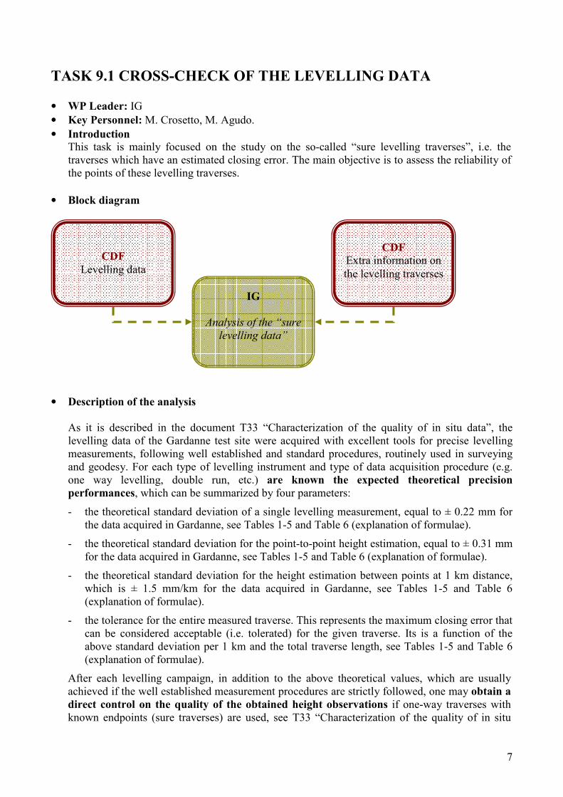
• Block diagram
• Description of the analysis
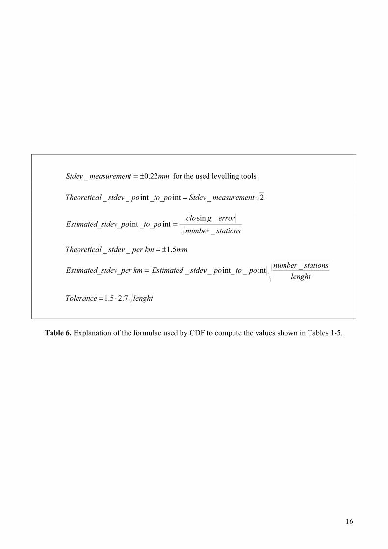
As it is described in the document T33 “Characterization of the quality of in situ data”, the levelling data of the Gardanne test site were acquired with excellent tools for precise levelling measurements, following well established and standard procedures, routinely used in surveying and geodesy. For each type of levelling instrument and type of data acquisition procedure (e.g. one way levelling, double run, etc.) are known the expected theoretical precision performances, which can be summarized by four parameters:
- the theoretical standard deviation of a single levelling measurement, equal to ± 0.22 mm for the data acquired in Gardanne, see Tables 1-5 and Table 6 (explanation of formulae).
- the theoretical standard deviation for the point-to-point height estimation, equal to ± 0.31 mm for the data acquired in Gardanne, see Tables 1-5 and Table 6 (explanation of formulae).
- the theoretical standard deviation for the height estimation between points at 1 km distance, which is ± 1.5 mm/km for the data acquired in Gardanne, see Tables 1-5 and Table 6 (explanation of formulae).
- the tolerance for the entire measured traverse. This represents the maximum closing error that can be considered acceptable (i.e. tolerated) for the given traverse. Its is a function of the above standard deviation per 1 km and the total traverse length, see Tables 1-5 and Table 6 (explanation of formulae).
After each levelling campaign, in addition to the above theoretical values, which are usually achieved if the well established measurement procedures are strictly followed, one may obtain a direct control on the quality of the obtained height observations if one-way traverses with known endpoints (sure traverses) are used, see T33 “Characterization of the quality of in situ
IG
Analysis of the “sure
levelling data”
CDF
Levelling data
CDF
Extra information on the levelling traverses

8
data”. In fact, for these traverses it is possible to estimate the closing error, a key experimental value (note, not a theoretical one) from which the following comparisons can be made. In order to accept a traverse the closing error must be smaller than the tolerance of the given traverse. Other parameters are given by the estimated standard deviation point-to-point (which can be compared with the theoretical standard deviation point-to-point), and the estimated standard deviation at 1 km (which can be compared with the theoretical standard deviation for the height estimation between at 1 km distance).
The Task 9.1 has been based on the extra information provided by Carbonnage De France, CDF. Thanks to this information, for the five sure levelling lines of the Gardanne test site, the above three comparisons have been made for each traverse. The results of the comparison of each traverse are briefly summarized below.
- The AXE levelling traverse (Table 1) represents the longest traverse, with a length up to 10.9 km (campaign of May 2000). With the exception of the first six campaigns, where the closing error is not available, all other 17 campaigns have a closing error that is smaller than the tolerance. This indicates the good quality of the data acquired with this traverse.
- The CIMETIÈRE levelling traverse (Table 2) is a much shorter traverse, with a length of about 2.5 km. With the exception of one campaign, all other 12 campaigns have a closing error that is smaller than the tolerance. The only exception (June 1995) shows a closing error that is 103% of the tolerance. This corresponds to an estimated standard deviation at 1 km of 4.2 mm/km. The quality of this traverse is certainly acceptable.
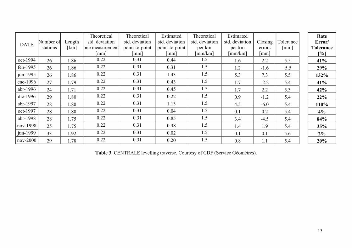
- The CENTRALE levelling traverse (Table 3) is a short traverse, with a length of about 1.8 km. Two campaigns out of 12 have a closing error above the tolerance (110% for April 1997, and 132% for June 1995). These two campaigns were however considered acceptable by CDF, and their data were included in the levelling dataset.
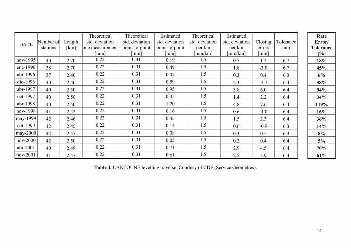
- The CANTOUNE levelling traverse (Table 4) has a length of about 2.5 km. For this traverse only one campaign out of 14 has a closing error above the tolerance (119% for April 1998). The quality of this traverse is globally acceptable.
- The BOUC levelling traverse (Table 5) has a length up to about 4 km. For this traverse all 14 campaigns have a closing error below the tolerance. Note that 6 of them have a ratio error/tolerance below 40%. This is certainly a good traverse.
In general the above traverses have a good quality. We focus the attention of other two key parameters to appreciate this quality:
- the estimated standard deviation point-to-point (which have typically a distance between 50 and 100 m) is well below 1 mm for almost all the levelling traverses, with very few exceptions for the above campaigns whose closing error is above the tolerance. This is an interesting parameter, which confirms the suitability of the analysed data even to validate the differential (point-to-point) deformation measures provided by PSI.
- another interesting parameter is given by the estimated standard deviation at 1 km, which for the great majority of the traverses (e.g. 14 out of 17 for the AXE traverse) is below 2 mm/km.
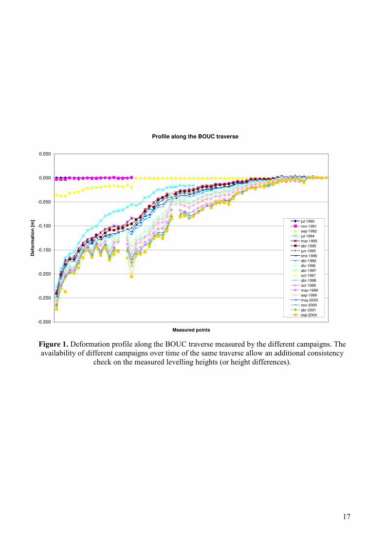
Beside the above parameters, which confirm the quality of the levelling data, one has to take into account that CDF had an additional important option to check the quality of the acquired data. In fact, thanks to the availability of different campaigns over the same traverse, for each campaign it was possible to check the consistency of its data with the data already acquired in previous

9
campaigns (an example of deformation profile along the BOUC traverse is shown in Figure 1): this represents an interesting extra-control to guarantee the quality of the acquired data. • The result of the analysis is POSITIVE
The analysis of the levelling traverses with estimated closing errors confirms the good global quality of the levelling data used as reference in the PSIC4 validation activities.
Note that an additional analysis on the quality of the levelling line has been carried out in the sub-task T9.2.2. This analysis concerns the planimetric positioning of the levelling points.


11
DATE Number of
stations
Length [km]
Theoretical std. deviation
one measurement [mm]
Theoretical std. deviation point-to-point
[mm]
Estimated std. deviation point-to-point
[mm]
Theoretical std. deviation
per km [mm/km]
Estimated std. deviation
per km [mm/km]
Closing errors [mm]
Tolerance [mm]
Rate
Error/
Tolerance
[%]
jul-1990 15 0.53 0.22 0.31 1.5 +/- 2.9 sep-1991 41 2.58 0.22 0.31 1.5 +/- 6.5 ago-1992 137 9.04 0.22 0.31 1.5 +/- 12.2 abr-1993 137 9.04 0.22 0.31 1.5 +/- 12.2 oct-1993 137 9.04 0.22 0.31 1.5 +/- 12.2 abr-1994 41 2.58 0.22 0.31 1.5 +/- 6.5 oct-1994 137 9.04 0.22 0.31 0.99 1.5 3.9 11.6 +/- 12.2 95%
feb-1995 139 9.01 0.22 0.31 0.30 1.5 1.2 3.5 +/- 12.2 29%
jun-1995 141 9.10 0.22 0.31 0.07 1.5 0.3 0.8 +/- 12.2 7%
ene-1996 140 8.97 0.22 0.31 0.35 1.5 1.4 -4.1 +/- 12.1 34%
abr-1996 143 9.18 0.22 0.31 0.53 1.5 2.1 -6.3 +/- 12.3 51%
dic-1996 172 9.18 0.22 0.31 0.26 1.5 1.1 -3.4 +/- 12.3 28%
abr-1997 173 9.18 0.22 0.31 0.37 1.5 1.6 -4.8 +/- 12.3 39%
oct-1997 173 9.18 0.22 0.31 0.23 1.5 1.0 -3.1 +/- 12.3 25%
abr-1998 175 9.18 0.22 0.31 0.37 1.5 1.6 -4.8 +/- 12.3 39%
oct-1998 153 9.32 0.22 0.31 0.15 1.5 0.6 +1.8 +/- 12.4 15%
abr-1999 173 10.24 0.22 0.31 0.47 1.5 1.9 -6.2 +/- 13.0 48%
sep-1999 142 8.04 0.22 0.31 0.07 1.5 0.3 -0.8 +/- 11.5 7%
may-2000 186 10.91 0.22 0.31 0.21 1.5 0.9 -2.9 +/- 13.4 22%
oct-2000 185 10.62 0.22 0.31 0.61 1.5 2.5 +8.3 +/- 13.2 63%
abr-2001 141 8.04 0.22 0.31 0.22 1.5 0.9 +2.6 +/- 11.5 23%
oct-2001 141 8.03 0.22 0.31 0.45 1.5 1.9 +5.3 +/- 11.5 46%
jun-2002 112 6.33 0.22 0.31 0.33 1.5 1.4 +3.5 +/- 10.2 34%
Table 1. AXE levelling traverse. Courtesy of CDF (Service Géomètres).

12
Table 2. CIMETIÈRE levelling traverse. Courtesy of CDF (Service Géomètres).
DATE Number of
stations
Length [km]
Theoretical std. deviation
one measurement [mm]
Theoretical std. deviation point-to-point
[mm]
Estimated std. deviation point-to-point
[mm]
Theoretical std. deviation
per km [mm/km]
Estimated std. deviation
per km [mm/km]
Closing errors [mm]
Tolerance [mm]
Rate
Error/
Tolerance
[%]
oct-1994 42 2.50 0.22 0.31 0.31 1.5 1.3 2.0 6.4 31%
feb-1995 43 2.50 0.22 0.31 0.46 1.5 1.9 3.0 6.4 47%
jun-1995 43 2.50 0.22 0.31 1.01 1.5 4.2 6.6 6.4 103%
ene-1996 45 2.50 0.22 0.31 0.48 1.5 2.0 -3.2 6.4 50%
abr-1996 45 2.59 0.22 0.31 0.02 1.5 0.1 0.2 6.5 2%
dic-1996 50 2.50 0.22 0.31 0.35 1.5 1.6 2.5 6.4 39%
abr-1997 47 2.50 0.22 0.31 0.76 1.5 3.3 5.2 6.4 81%
oct-1997 48 2.50 0.22 0.31 0.68 1.5 3.0 4.7 6.4 73%
abr-1998 48 2.50 0.22 0.31 0.84 1.5 3.7 5.8 6.4 91%
nov-1998 44 2.53 0.22 0.31 0.39 1.5 1.6 -2.6 6.4 40%
jun-1999 52 2.54 0.22 0.31 0.07 1.5 0.3 -0.5 6.5 8%
jun-2000 48 2.58 0.22 0.31 0.43 1.5 1.9 3.0 6.5 46%
nov-2000 49 2.57 0.22 0.31 0.07 1.5 0.3 0.5 6.5 8%
13
DATE Number of
stations
Length [km]
Theoretical std. deviation
one measurement [mm]
Theoretical std. deviation point-to-point
[mm]
Estimated std. deviation point-to-point
[mm]
Theoretical std. deviation
per km [mm/km]
Estimated std. deviation
per km [mm/km]
Closing errors [mm]
Tolerance [mm]
Rate
Error/
Tolerance
[%]
oct-1994 26 1.86 0.22 0.31 0.44 1.5 1.6 2.2 5.5 41%
feb-1995 26 1.86 0.22 0.31 0.31 1.5 1.2 -1.6 5.5 29%
jun-1995 26 1.86 0.22 0.31 1.43 1.5 5.3 7.3 5.5 132%
ene-1996 27 1.79 0.22 0.31 0.43 1.5 1.7 -2.2 5.4 41%
abr-1996 24 1.71 0.22 0.31 0.45 1.5 1.7 2.2 5.3 42%
dic-1996 29 1.80 0.22 0.31 0.22 1.5 0.9 -1.2 5.4 22%
abr-1997 28 1.80 0.22 0.31 1.13 1.5 4.5 -6.0 5.4 110%
oct-1997 28 1.80 0.22 0.31 0.04 1.5 0.1 0.2 5.4 4%
abr-1998 28 1.75 0.22 0.31 0.85 1.5 3.4 -4.5 5.4 84%
nov-1998 25 1.75 0.22 0.31 0.38 1.5 1.4 1.9 5.4 35%
jun-1999 33 1.92 0.22 0.31 0.02 1.5 0.1 0.1 5.6 2%
nov-2000 29 1.78 0.22 0.31 0.20 1.5 0.8 1.1 5.4 20%
Table 3. CENTRALE levelling traverse. Courtesy of CDF (Service Géomètres).
14
DATE Number of
stations
Length [km]
Theoretical std. deviation
one measurement [mm]
Theoretical std. deviation point-to-point
[mm]
Estimated std. deviation point-to-point
[mm]
Theoretical std. deviation
per km [mm/km]
Estimated std. deviation
per km [mm/km]
Closing errors [mm]
Tolerance [mm]
Rate
Error/
Tolerance
[%]
nov-1995 40 2.70 0.22 0.31 0.19 1.5 0.7 1.2 6.7 18%
ene-1996 38 2.70 0.22 0.31 0.49 1.5 1.8 -3.0 6.7 45%
abr-1996 37 2.40 0.22 0.31 0.07 1.5 0.3 0.4 6.3 6%
dic-1996 40 2.50 0.22 0.31 0.59 1.5 2.3 -3.7 6.4 58%
abr-1997 40 2.50 0.22 0.31 0.95 1.5 3.8 6.0 6.4 94%
oct-1997 40 2.50 0.22 0.31 0.35 1.5 1.4 2.2 6.4 34%
abr-1998 40 2.50 0.22 0.31 1.20 1.5 4.8 7.6 6.4 119%
nov-1998 41 2.52 0.22 0.31 0.16 1.5 0.6 -1.0 6.4 16%
may-1999 42 2.46 0.22 0.31 0.35 1.5 1.5 2.3 6.4 36%
oct-1999 42 2.45 0.22 0.31 0.14 1.5 0.6 -0.9 6.3 14%
may-2000 44 2.45 0.22 0.31 0.08 1.5 0.3 0.5 6.3 8%
nov-2000 42 2.50 0.22 0.31 0.05 1.5 0.2 0.4 6.4 5%
abr-2001 40 2.49 0.22 0.31 0.71 1.5 2.9 4.5 6.4 70%
nov-2001 41 2.47 0.22 0.31 0.61 1.5 2.5 3.9 6.4 61%
Table 4. CANTOUNE levelling traverse. Courtesy of CDF (Service Géomètres).

15
DATE Number of
stations
Length [km]
Theoretical std. deviation
one measurement [mm]
Theoretical std. deviation point-to-point
[mm]
Estimated std. deviation point-to-point
[mm]
Theoretical std. deviation
per km [mm/km]
Estimated std. deviation
per km [mm/km]
Closing errors [mm]
Tolerance [mm]
Rate
Error/
Tolerance
[%]
abr-1995 47 3.72 0.22 0.31 0.12 1.5 0.4 -0.8 7.8 10%
jun-1995 47 3.72 0.22 0.31 0.71 1.5 2.5 4.9 7.8 63%
ene-1996 48 3.80 0.22 0.31 0.12 1.5 0.4 0.8 7.9 10%
abr-1996 47 3.70 0.22 0.31 1.12 1.5 4.0 -7.7 7.8 99%
dic-1996 60 3.90 0.22 0.31 0.08 1.5 0.3 -0.6 8.0 8%
abr-1997 60 3.90 0.22 0.31 0.63 1.5 2.5 4.9 8.0 61%
oct-1997 60 3.90 0.22 0.31 0.01 1.5 0.0 -0.1 8.0 1%
abr-1998 60 3.90 0.22 0.31 0.99 1.5 3.9 7.7 8.0 96%
oct-1998 59 3.89 0.22 0.31 0.10 1.5 0.4 -0.8 8.0 10%
may-1999 60 4.00 0.22 0.31 0.27 1.5 1.1 -2.1 8.1 26%
sep-1999 54 3.80 0.22 0.31 0.08 1.5 0.3 -0.6 7.9 7%
may-2000 51 3.80 0.22 0.31 0.06 1.5 0.2 0.4 7.9 5%
nov-2000 51 3.80 0.22 0.31 1.02 1.5 3.7 7.3 7.9 92%
abr-2001 51 3.80 0.22 0.31 0.18 1.5 0.7 1.3 7.9 16%
Table 5. BOUC levelling traverse. Courtesy of CDF (Service Géomètres).
16
mmtmeasuremenStdev 22.0_ ±= for the used levelling tools
2_intint__ tmeasuremenStdev_to_popostdevlTheoretica =
stationsnumber
errorgclo_to_postdev_poEstimated_
_
_sinintint =
mmper kmstdevlTheoretica 5.1__ ±=
lenght
stationsnumberpotopostdevEstimatedkmstdev_per Estimated_
_int_int___=
lenghtTolerance 7.25.1 ⋅=
Table 6. Explanation of the formulae used by CDF to compute the values shown in Tables 1-5.
17
Profile along the BOUC traverse
-0.300
-0.250
-0.200
-0.150
-0.100
-0.050
0.000
0.050
Measured points
Defo
rmati
on
[m
] jul-1990
nov-1991
sep-1992
jul-1994
mar-1995
abr-1995
jun-1995
ene-1996
abr-1996
dic-1996
abr-1997
oct-1997
abr-1998
oct-1998
may-1999
sep-1999
may-2000
nov-2000
abr-2001
sep-2004
Figure 1. Deformation profile along the BOUC traverse measured by the different campaigns. The availability of different campaigns over time of the same traverse allow an additional consistency
check on the measured levelling heights (or height differences).

18
TASK 9.2 REVIEW THE PRE-PROCESSING OPERATIONS
• WP Leader: IG • Key Personnel: M. Crosetto, M. Agudo. • Sub-tasks:
� T9.2.1 Consistency check of the different input datasets
� T9.2.2 Check of coordinate transformation
� T9.2.3 Review how geocoding errors are estimated and corrected
� T9.2.4 Review how deformations are referred to the same area
� T9.2.5 Review the spatial resampling of PS dataT9.2.6 Review the temporal
resampling of levelling data
T9.2.6 Review the temporal
resampling of levelling data
T9.2.5 Review the
spatial resampling of
PS data T9.2.4
Review how deformations are referred to the same area
T9.2.3 Review how geocoding errors are
estimated and corrected
T9.2.2
Check of coordinate
transformation
T9.2.1
Consistency check of the
different input datasets
T9.2
Pre-processing
operations

19
TASK 9.2.1 CONSISTENCY CHECK OF THE DIFFERENT INPUT
DATASETS
• WP Leader: IG • Key Personnel: M. Crosetto, M. Agudo. • Introduction
Generic check on the different data gathered from CDF, the PSI teams, and other sources.
• Block diagram - Check the levelling points (see Task 9.2.2.1). - Check the orthoimage (see Task 9.2.2.2). - Check the levelling points over the orthoimage (see Task 9.2.2.3). - Check the PS datasets.
Levelling
points
BRGM
Compile the different
datasets
Consistency of the different input datasets
(See Task 9.2.2)
PS in WGS84 coordinates
provided by ESA (coming from the
teams)
Orthoimage
Auxiliary data, mining maps, etc.
Check 1
Check 2
20
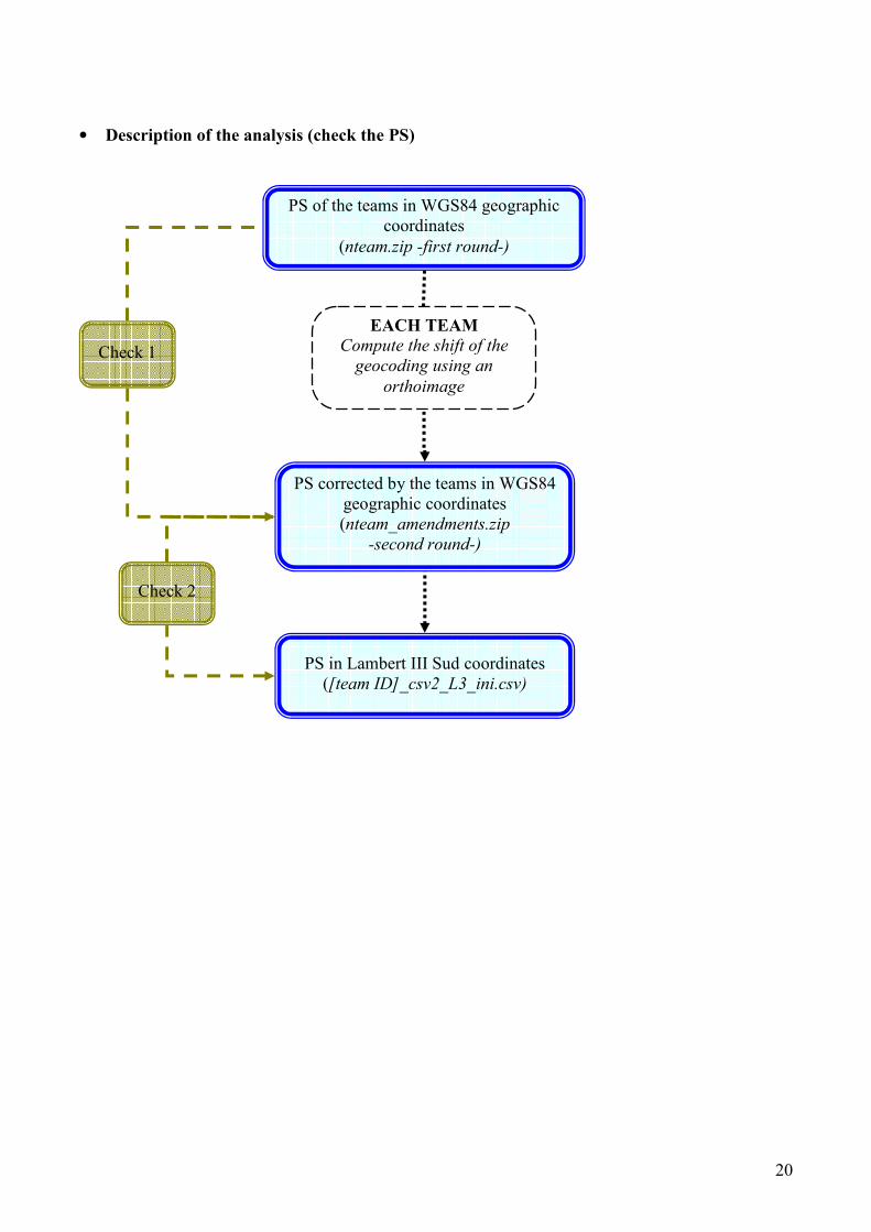
• Description of the analysis (check the PS)
PS of the teams in WGS84 geographic coordinates
(nteam.zip -first round-)
EACH TEAM
Compute the shift of the
geocoding using an
orthoimage
PS corrected by the teams in WGS84 geographic coordinates (nteam_amendments.zip
-second round-)
Check 1
Check 2
PS in Lambert III Sud coordinates ([team ID]_csv2_L3_ini.csv)
21
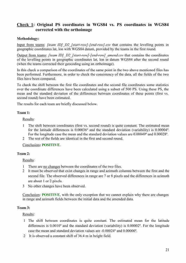
Check 1: Original PS coordinates in WGS84 vs. PS coordinates in WGS84
corrected with the orthoimage
Methodology:
Input from teams: [team ID]_D2_[start-row]-[end-row].csv that contains the levelling points in geographic coordinates lat, lon with WGS84 datum, provided by the teams in the first round.
Output from teams: [team ID]_D2_[start-row]-[end-row]_amend.csv that contains the coordinates of the levelling points in geographic coordinates lat, lon in datum WGS84 after the second round (when the teams corrected their geocoding using an orthoimage).
In this check a comparison of the coordinates of the same point in the two above mentioned files has been performed. Furthermore, in order to check the consistency of the data, all the fields of the two files have been compared.
To check the shift between the first file coordinates and the second file coordinates some statistics over the coordinate differences have been calculated using a subset of 500 PS. Using these PS, the mean and the standard deviation of the differences between coordinates of these points (first vs. second round) have been estimated.
The results for each team are briefly discussed below.
Team 1:
Results:
1 The shift between coordinates (first vs. second round) is quite constant. The estimated mean for the latitude differences is 0.00036º and the standard deviation (variability) is 0.00004º. For the longitude case the mean and the standard deviation values are 0.00049º and 0.00028º.
2 The rest of the fields are identical in the first and second round.
Conclusion: POSITIVE.
Team 2:
Results:
1 There are no changes between the coordinates of the two files. 2 It must be observed that exist changes in range and azimuth columns between the first and the
second file. The observed differences in range are 7 or 8 pixels and the differences in azimuth are about 1 or 2 pixels.
3 No other changes have been observed.
Conclusion: POSITIVE, with the only exception that we cannot explain why there are changes in range and azimuth fields between the initial data and the amended data.
Team 3:
Results:
1 The shift between coordinates is quite constant. The estimated mean for the latitude differences is 0.0010º and the standard deviation (variability) is 0.00002º. For the longitude case the mean and standard deviation values are -0.00024º and 0.00000º.
2 It is observed a constant shift of 36.4 m in height field.

22
3 No more changes have been observed.
Conclusion: POSITIVE.
Team 4:
Results:
1 The shift between coordinates is constant. The constant shifts are in latitude 0.00004º and in longitude 0.00013º.
2 There are constant shifts in the range coordinates (1160 pixels) and in azimuth ones (14250). 3 No more changes have been observed.
Conclusion: POSITIVE, with the exception that we cannot explain why there are changes in range and azimuth fields between initial data and amended data.
Team 5:
Results:
1 The shift between coordinates is quite constant. The estimated mean for the latitude differences is -0.00014º and the standard deviation (variability) is 0.00003º. For the longitude case the mean and standard deviation values are -0.00017º and 0.00019º.
2 It is observed a high variability in height field and in range field.
Conclusion: POSITIVE, with the exception that we cannot explain why there are changes in range and azimuth fields between initial data and amended data.
Team 6:
Results:
1 There are no changes between the coordinates of the two files. 2 It must be observed that there are changes in range and azimuth colons between the first and
the second file. The observed differences in range are 5 pixels and the differences in azimuth are of 161 pixels.
3 No more changes have been observed.
Conclusion: POSITIVE.
Team 7:
Results:
No amendments were provided by Team 7.
Team 8:
Results:
It seems that the data have been entirely re-processed. Therefore, this check for Team 8 has no meaning.
In the following, a table summarizes all the shifts obtained by the correction of the teams from the first round to the second round.
23
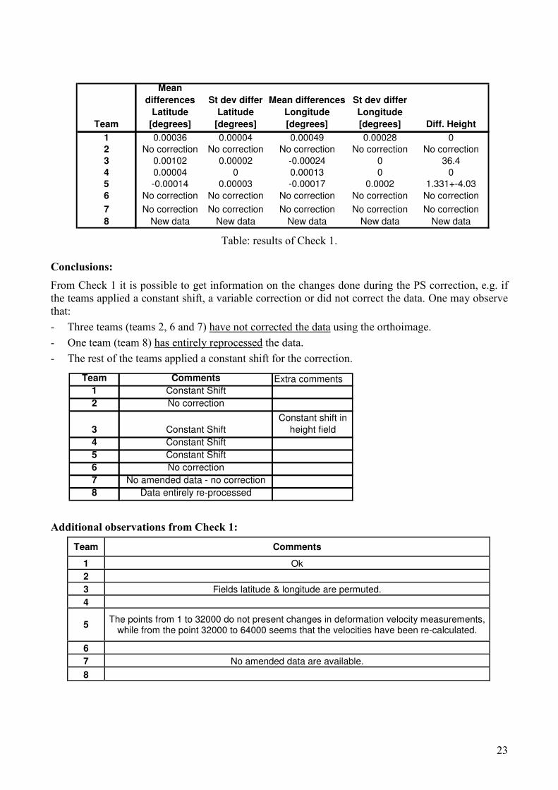
Table: results of Check 1.
Conclusions:
From Check 1 it is possible to get information on the changes done during the PS correction, e.g. if the teams applied a constant shift, a variable correction or did not correct the data. One may observe that:
- Three teams (teams 2, 6 and 7) have not corrected the data using the orthoimage.
- One team (team 8) has entirely reprocessed the data.
- The rest of the teams applied a constant shift for the correction.
Additional observations from Check 1:
Team Comments
1 Ok
2
3 Fields latitude & longitude are permuted.
4
5 The points from 1 to 32000 do not present changes in deformation velocity measurements,
while from the point 32000 to 64000 seems that the velocities have been re-calculated.
6
7 No amended data are available.
8
Team
Mean
differences
Latitude
[degrees]
St dev differ
Latitude
[degrees]
Mean differences
Longitude
[degrees]
St dev differ
Longitude
[degrees] Diff. Height
1 0.00036 0.00004 0.00049 0.00028 0
2 No correction No correction No correction No correction No correction
3 0.00102 0.00002 -0.00024 0 36.4
4 0.00004 0 0.00013 0 0
5 -0.00014 0.00003 -0.00017 0.0002 1.331+-4.03
6 No correction No correction No correction No correction No correction
7 No correction No correction No correction No correction No correction
8 New data New data New data New data New data
Team Comments Extra comments
1 Constant Shift
2 No correction
3 Constant Shift
Constant shift in
height field
4 Constant Shift
5 Constant Shift
6 No correction
7 No amended data - no correction
8 Data entirely re-processed
24
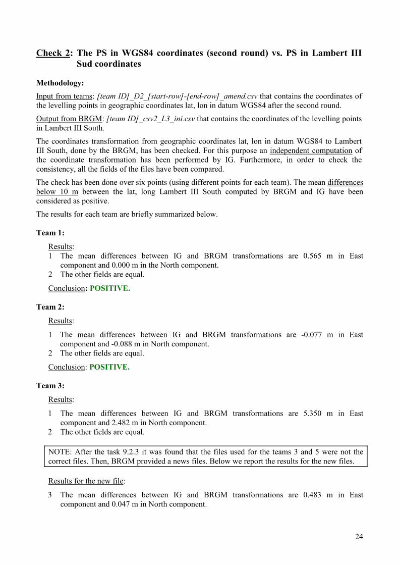
Check 2: The PS in WGS84 coordinates (second round) vs. PS in Lambert III
Sud coordinates
Methodology:
Input from teams: [team ID]_D2_[start-row]-[end-row]_amend.csv that contains the coordinates of the levelling points in geographic coordinates lat, lon in datum WGS84 after the second round.
Output from BRGM: [team ID]_csv2_L3_ini.csv that contains the coordinates of the levelling points in Lambert III South.
The coordinates transformation from geographic coordinates lat, lon in datum WGS84 to Lambert III South, done by the BRGM, has been checked. For this purpose an independent computation of the coordinate transformation has been performed by IG. Furthermore, in order to check the consistency, all the fields of the files have been compared.
The check has been done over six points (using different points for each team). The mean differences below 10 m between the lat, long Lambert III South computed by BRGM and IG have been considered as positive.
The results for each team are briefly summarized below. Team 1:
Results: 1 The mean differences between IG and BRGM transformations are 0.565 m in East
component and 0.000 m in the North component. 2 The other fields are equal.
Conclusion: POSITIVE.
Team 2:
Results:
1 The mean differences between IG and BRGM transformations are -0.077 m in East component and -0.088 m in North component.
2 The other fields are equal.
Conclusion: POSITIVE.
Team 3:
Results:
1 The mean differences between IG and BRGM transformations are 5.350 m in East component and 2.482 m in North component.
2 The other fields are equal. NOTE: After the task 9.2.3 it was found that the files used for the teams 3 and 5 were not the correct files. Then, BRGM provided a news files. Below we report the results for the new files.
Results for the new file:
3 The mean differences between IG and BRGM transformations are 0.483 m in East component and 0.047 m in North component.

25
4 The other fields are equal.
Conclusion: POSITIVE.
Team 4:
Results:
1 The mean differences between IG and BRGM transformations are -0.044 m in East component and -0.084 m in North component.
2 The other fields are equal.
Conclusion: POSITIVE.
Team 5:
Results:
1 The mean differences between IG and BRGM transformations are -8.477 m in East component and 1.657 m in North component.
2 The other fields are equal. NOTE: After the task 9.2.3 it was found that the files used for the teams 3 and 5 were not the correct files. Then, BRGM provided a news files. Below we report the results for the new files.
Results for the new file:
3 The mean differences between IG and BRGM transformations are 0.790 m in East component and 0.113 m in North component.
4 The other fields are equal. Conclusion: POSITIVE.
Team 6:
Results:
1 The mean differences between IG and BRGM transformations are -0.099 m in East component and -0.104 m in North component.
2 The other fields are equal.
Conclusion: POSITIVE.
Team 7:
Results:
1 The mean differences between IG and BRGM transformations are -0.076 m in East component and -0.081 m in North component.
2 The other fields are equal.
Conclusion: POSITIVE.

26
Team 8:
Results:
1 The mean differences between IG and BRGM transformations are 0.491 m in East component and 0.048 m in North component.
2 The other fields are equal.
Conclusion: POSITIVE.
The following table summarizes the differences estimated for the eight teams.
Team Mean
differences East (m)
Mean differences North (m)
Dif Heigh
Dif. velo
Dif. cohe
Dif. range
Dif. azimut
1 0.565 0.000 0.000 0.000 0.000 0.000 0.000
2 -0.077 -0.088 0.000 0.000 0.000 0.000 0.000
3 0.483 0.046 0.000 0.000 0.000 0.000 0.000
4 -0.044 -0.084 0.000 0.000 0.000 0.000 0.000
5 0.790 0.113 0.000 0.000 0.000 0.000 0.000
6 -0.099 -0.104 0.000 0.000 0.000 0.000 0.000
7 -0.076 -0.081 0.000 0.000 0.000 0.000 0.000
8 0.491 0.048 0.000 0.000 0.000 0.000 0.000
Table: results of Check 2.

27
TASK 9.2.2 CHECK OF COORDINATE TRANSFORMATION
• WP Leader: IG • Key Personnel: M. Crosetto, M. Agudo. • Introduction
Generic check on the different datasets which have undergone coordinate transformation. • Block diagram
PS datasets in WGS84
Levelling coordinates in Lambert III Sud
Coordinate transformation from WGS84 or Lambert II etendú to
Lambert III Sud
Levelling over the orthoimage (in Lambert III Sud
coordinates)
Orthoimages in Lambert II etendú and WGS84
PS datasets over the orthoimage (in Lambert III Sud
coordinates)
See sub-task 9.2.2.1
See Task 9.2.1
See sub-task 9.2.2.2
See sub-task 9.2.2.3
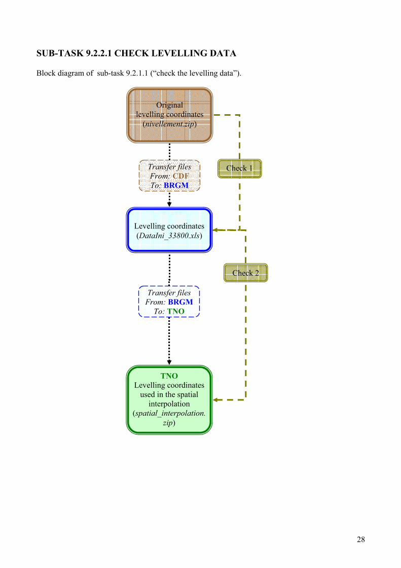
28
SUB-TASK 9.2.2.1 CHECK LEVELLING DATA
Block diagram of sub-task 9.2.1.1 (“check the levelling data”).
Original
levelling coordinates (nivellement.zip)
Transfer files
From: CDF
To: BRGM
Levelling coordinates (DataIni_33800.xls)
TNO
Levelling coordinates used in the spatial
interpolation (spatial_interpolation.
zip)
Transfer files
From: BRGM
To: TNO
Check 1
Check 2

29
Preliminary Check:
In a preliminary Check, we observed that exist several levelling points with the same coordinates. In order to check if this, some questions were sent to CDF (Carbonnage de France).
Step 1: Questions for CDF
In the files Puits_y.xls and Arbois.xls we found these points with the same coordinates. Can you please explain why? See the mentioned points in the following tables.
� Line Puits_y:
Y--1--Sud-Est 851777 132777Y--10--Sud-est 851777 132777… … … … … … … … … Y--2--Nord-Est 851798 132768Y--20--Nord-Est 851798 132768Y--21--Nord-Est 851798 132768… … … … … … Y--31--Nord-Ouest 851790 132752Y--30--Nord-Ouest 851790 132752
� Line Arbois:
12--540 851335 133592 12--541-1 851335 133592 … … … 12--550 851325 133590 12--551-1 851325 133590
Step 2: Response from CDF
There are some points with the same coordinates because in some places a redundant information is needed: two or more levelling points can be located within few tens of centimetres. Therefore, the information contained in the files is correct. The result of this preliminary Check was therefore considered POSITIVE.

30
Check 1: The levelling coordinates CDF vs. BRGM In order to control the planimetric coordinates of the levelling points, a check has been realized in order to ensure that the levelling coordinates didn’t suffered any change during the file transformation from CDF to BRGM. Methodology:
Input from CDF: levelling.zip that contains 12 Excel files with the original Lambert III Sud coordinates for the levelling lines.
Input from BRGM: Dataini_33800.xls that contains the coordinates of the levelling points in Lambert III Sud coordinates.
Comparison of the coordinates of the same point in the two files coming from different groups. Results:
1. For the 12 levelling lines the comparison was satisfactory. Some difference exist between
the two files, but the differences are negligible if compared with the precision of the levelling measurements.
2. In different levelling lines there are points of the CDF file that have not been included in the
BRGM file.
Conclusion: POSITIVE.
Details of the analysis check:
This is the list of the analysed levelling lines: Axe, Cantoune, Centrale, Cimetiere, Hbcm_bouc, Arbois, Pechiney_usine, Puits_y, Scp_bouc, Scp_maillage, Scp_simiane, Sncf_aix_marxeille. The first five lines are the closed levelling lines.
In the Annex 1 of this document are reported the results of Check 1 for the closed levelling lines. The results for the rest of the lines are reported in the Annex 1.2. For each line are shown the X, Y Lambert III South coordinates for the points coming from the CDF files and those for the BRGM file. In the two last columns are shown the difference between the X and the Y coordinates respectively.

31
Check 2: The levelling coordinates used in the spatial interpolation compared
with the BRGM coordinates The BRGM and TNO files (Dataini_33800.xls and spatial_interpolation.zip, respectively) contain in principle the same coordinates for the levelling points.
In order to control the levelling coordinates used in the spatial interpolation, a comparison with the BRGM files checked in Check 1 has been realized. Methodology:
Input from BRGM: Dataini_33800.xls that contains the coordinates of the levelling points in Lambert III Sud coordinates.
Input from TNO: spatial_interpolation.zip.
It has been done a comparison of the coordinates of the same points in the two above mentioned files and has been computed the difference in the same way done in Check 1. Results:
There are no differences between the two files. There is a full consistency between the input and the output files.
Conclusion: POSITIVE.

32
SUB-TASK 9.2.2.2 CHECK THE ORTHOIMAGE
Block diagram of sub-task 9.2.2.2 (“check the orthoimage”).
Orthoimage in Lambert II Sud coordinates
(13-1998-820-1835-C10.ecw
13-1998-820-1870-C10.ecw
- for the validation tasks -)
Orthoimage in Lambert III Sud coordinates
(SUD_lambertIIIS_2.tif -for the
validation tasks on the Gardanne area)
Orthoimage in WGS84 coordinates (SUD_WGS84_6_urbanarea2.tif –
provided to the teams)
Check
33
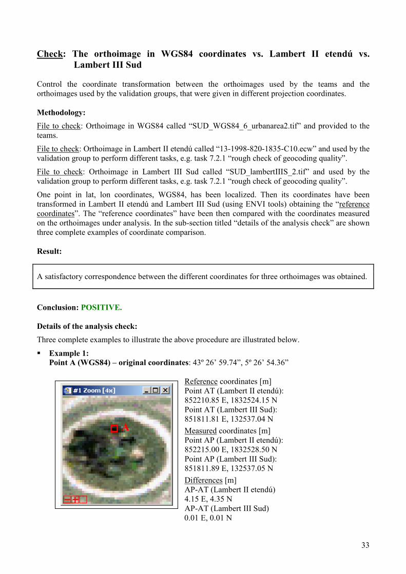
Check: The orthoimage in WGS84 coordinates vs. Lambert II etendú vs.
Lambert III Sud Control the coordinate transformation between the orthoimages used by the teams and the orthoimages used by the validation groups, that were given in different projection coordinates. Methodology:
File to check: Orthoimage in WGS84 called “SUD_WGS84_6_urbanarea2.tif” and provided to the teams.
File to check: Orthoimage in Lambert II etendú called “13-1998-820-1835-C10.ecw” and used by the validation group to perform different tasks, e.g. task 7.2.1 “rough check of geocoding quality”.
File to check: Orthoimage in Lambert III Sud called “SUD_lambertIIIS_2.tif” and used by the validation group to perform different tasks, e.g. task 7.2.1 “rough check of geocoding quality”.
One point in lat, lon coordinates, WGS84, has been localized. Then its coordinates have been transformed in Lambert II etendú and Lambert III Sud (using ENVI tools) obtaining the “reference coordinates”. The “reference coordinates” have been then compared with the coordinates measured on the orthoimages under analysis. In the sub-section titled “details of the analysis check” are shown three complete examples of coordinate comparison. Result:
A satisfactory correspondence between the different coordinates for three orthoimages was obtained.
Conclusion: POSITIVE.
Details of the analysis check:
Three complete examples to illustrate the above procedure are illustrated below.
� Example 1:
Point A (WGS84) – original coordinates: 43º 26’ 59.74”, 5º 26’ 54.36”
Reference coordinates [m] Point AT (Lambert II etendú): 852210.85 E, 1832524.15 N Point AT (Lambert III Sud): 851811.81 E, 132537.04 N
Measured coordinates [m] Point AP (Lambert II etendú): 852215.00 E, 1832528.50 N Point AP (Lambert III Sud): 851811.89 E, 132537.05 N
Differences [m] AP-AT (Lambert II etendú) 4.15 E, 4.35 N AP-AT (Lambert III Sud)
0.01 E, 0.01 N
A

34
Lambert III Sud: Lambert II etendú:
� Example 2:
Point B (WGS84) – original coordinates: 43º 27’ 7.00”, 5º 27’ 23.54”
Reference coordinates [m] Point BT (Lambert II etendú): 852858.55 E, 1832774.41 N Point BT(Lambert III Sud): 852458.91 E, 132785.74 N Measured coordinates [m] Point BP (Lambert II etendú): 852863.00 E, 1832778.00 N Point BP(Lambert III Sud): 852458.89 E, 132785.55 N Differences [m] BP-BT (Lambert II etendú) 4.45 E, 3.59 N BP-BT (Lambert III Sud) -0.02 E, -0.19 N
B
AT=AP
AT
AP
35
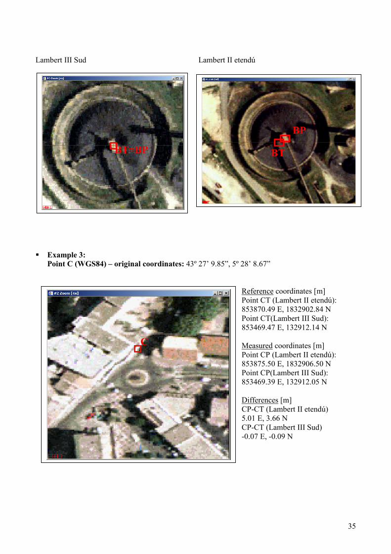
Lambert III Sud Lambert II etendú
� Example 3:
Point C (WGS84) – original coordinates: 43º 27’ 9.85”, 5º 28’ 8.67”
Reference coordinates [m] Point CT (Lambert II etendú): 853870.49 E, 1832902.84 N Point CT(Lambert III Sud): 853469.47 E, 132912.14 N Measured coordinates [m] Point CP (Lambert II etendú): 853875.50 E, 1832906.50 N Point CP(Lambert III Sud): 853469.39 E, 132912.05 N Differences [m] CP-CT (Lambert II etendú) 5.01 E, 3.66 N CP-CT (Lambert III Sud) -0.07 E, -0.09 N
BT=BP
BT
BP
C

36
Lambert III Sud: Lambert II etendú:
CT = CP
CT CP
37
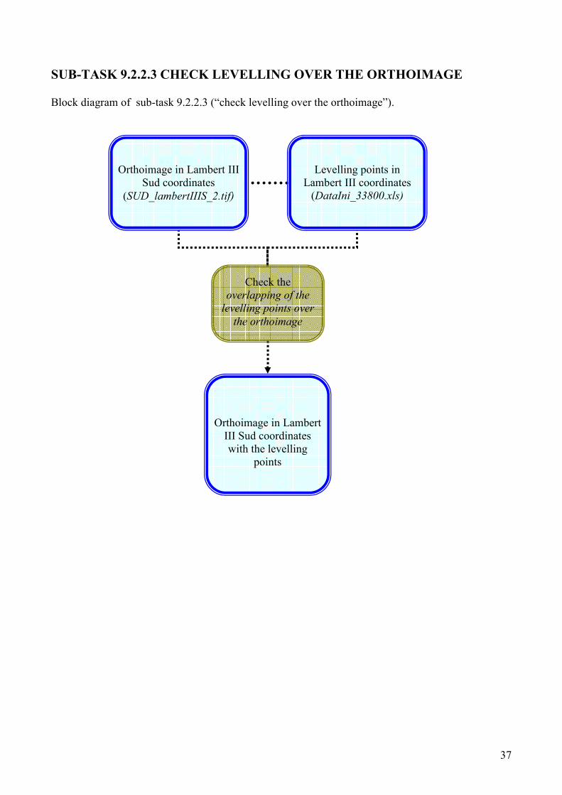
SUB-TASK 9.2.2.3 CHECK LEVELLING OVER THE ORTHOIMAGE
Block diagram of sub-task 9.2.2.3 (“check levelling over the orthoimage”).
Orthoimage in Lambert III Sud coordinates
(SUD_lambertIIIS_2.tif)
Check the overlapping of the
levelling points over
the orthoimage
Orthoimage in Lambert III Sud coordinates with the levelling
points
Levelling points in Lambert III coordinates
(DataIni_33800.xls)

38
Check: The levelling coordinates over the orthoimage In order to check the planimetric position of the levelling points, these points have been overlapped to the orthoimage. In order to control the accurate position of these points, an independent check over the closed levelling lines has been realized by CDF. Methodology :
Input from BRGM: Dataini_33800.xls that contains the coordinates of the levelling points in Lambert III Sud coordinates.
Input from BRGM: SUD_lambertIIIS_2.tif orthoimage in Lambert III Sud coordinates.
Files to check: Axe.doc, Cantoune.doc, Centrale.doc, Cimetiere.doc, Hbcm_bouc.doc. Independent check through CDF:
First step: In order to control the location of the levelling various files with the levelling points overlapped to the orthoimage have been generated. An independent check has been realized by sending these files to CDF.
Results of first step: The response from CDF was satisfactory: only a negligible shift in the location of the levelling points was noticed.
Second step: A global check has been realized for the closed levelling lines. CDF sent to IG five PDF files with the levelling points overlapped to the orthoimage. This made possible the visual check of the levelling locations.
Result:
A satisfactory check has been realized. The shift that it could be appreciated is negligible for the purposes of the PSIC4 project.
Conclusion: POSITIVE.
Details of the analysis check:
The details of this check are shown in the Annex 2 of this document.

39
TASK 9.2.3 REVIEW HOW THE GEOCODING ERRORS ARE ESTIMATED
AND CORRECTED
• WP Leader: IG • Key Personnel: M. Crosetto, M. Agudo. • Introduction
Verification of the geocoding error estimation procedure, check of the estimated systematic errors, and control of the procedure used to compensate for these errors.
• Block diagram
PS in Lambert III Sud coordinates for each
team (Tn_csv2_L3_ini.csv)
Transform files
From: BRGM
To: BRGM
PS corrected by the shifts computed by BRGM
(Tn_csv2_L3_Geocomp.csv)
Statistics and interpretation of the results for each team
Comparison
BRGM vs. BGS
Check 1
Check 2

40
Check 1: Formal check of the input files In order to control the files used and handled by BRGM, a formal check of all the fields included in these files has been realized. Furthermore, using the information of the coordinates of the PS before the correction of the BRGM estimations, i.e. the files provided by the teams ( “Tn_csv2_L3_ini.csv” ), and the information coming from the BRGM files the shifts applied to the teams has been checked against the BRGM documentation ( “Tn_csv2_L3_Geocomp.csv ” ). Methodology:
Input from BRGM: Tn_csv2_L3_ini.csv that contains the coordinates of the PS points in Lambert III Sud coordinates.
Output from BRGM: Tn_csv2_L3_Geocomp.csv that contains the coordinates of the PS points in Lambert III Sud coordinates and corrected with the geocoded shifts computed by BRGM. Results:
The shifts computed for the BRGM and the shifts founded in the documentation are consistent.
Conclusion: POSITIVE.
Details of the analysis check:
Comparison between the two files for each team:
TEAM
DIFF. X provided by
BRGM documentation
[m]
DIFF. Y provided by
BRGM documentation
[m]
Distance [m]
DIFF. X in PS_geocomp
FILEs [m]
DIFF. Y in PS_geocomp
FILEs [m]
COMMENTS
1 No reliable correspondence No changes -
2 15.35 -2.21 15.51 15.35 -2.21 -
3 7 4 8.06 0 0 No correspondence
with the files
4 13.88 4 14.44 13.88 4 -
5 7 -7 9.90 -0.53 -0.14 No correspondence
with the files
6 -79.36 21.12 82.12 -79.36 21.12
The no correction in the 2nd round could
explain the 80 m of the shift.
7 10.51 10.62 14.94 10.51 10.62 -
8 No reliable correspondence No changes -
After these results, the BRGM send two new files for teams 3 and 5 because the check indicated that something was wrong (see the comments in the last column of the above table). Therefore, a new difference table has been generated, see next page. It must be underline that the documentation of the shifts has changed. A new table with the computed shifts was used.
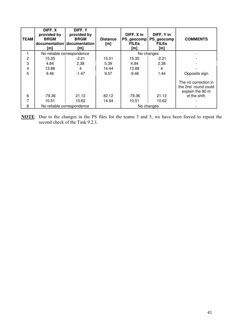
41
TEAM
DIFF. X provided by
BRGM documentation
[m]
DIFF. Y provided by
BRGM documentation
[m]
Distance [m]
DIFF. X in PS_geocomp
FILEs [m]
DIFF. Y in PS_geocomp
FILEs [m]
COMMENTS
1 No reliable correspondence No changes -
2 15.35 -2.21 15.51 15.35 -2.21 -
3 4.84 2.38 5.39 4.84 2.38 -
4 13.88 4 14.44 13.88 4 -
5 9.46 -1.47 9.57 -9.46 1.44 Opposite sign
6 -79.36 21.12 82.12 -79.36 21.12
The no correction in the 2nd. round could
explain the 80 m of the shift.
7 10.51 10.62 14.94 10.51 10.62 -
8 No reliable correspondence No changes -
NOTE: Due to the changes in the PS files for the teams 3 and 5, we have been forced to repeat the
second check of the Task 9.2.1.

42
Check 2: Check how the geocoding errors are corrected and estimated In a first step two checks related to the correction of the geocoded PS it have been performed. One of these check has been related to the files provided by BRGM that contained the final shifts applied to the teams. Check 2 involves an independent check over the files provided by BGS. Methodology:
Input from BRGM: “PSIC4 Report on the geocoding method.doc” that contains the information of the studies realized by BRGM for the geocoding correction.
Input from BGS: PS_Shifting_DraftReport1.doc that contains the information of the points used to compute the geocoding correction.
A comparison between the two studies has been done. One study is coming from BRGM and the other one from BGS. Furthermore, a visual check has been done in order to confirm that for the teams 1 and 8 it was impossible to determine the geocoding shifts. Result:
By comparing the geocoding shifts of BRGM and BGS we conclude that the geocoding corrections applied by BRGM to the PS teams (in the second delivery) are good corrections to establish a consistent relationship between the PS and the levelling points. Furthermore, from the interpretation of the geocoding results the following aspects were highlighted: - at least one team has excellent geocoding results (team 3); - other teams (like teams 4 and 5) have relatively good geocoding results. However, it is important
to underline that a there is a high dispersion of the estimated geocoding errors. This suggests to be careful in interpreting the magnitude of the geocoding errors.
- one team has big geocoding errors (team 6). However, one has to consider that this team has not performed the correction of the geocoding based on the orthoimage (second round).
Conclusion: POSITIVE.
Details of the analysis check:
For each team we have visualized the corrected PS over the orthoimage. Furthermore, some statistics have been computed using the documentation coming from the BGS study related to the rough geocoding. The most important results are briefly commented below. Some other details of the analysis are reported in the Annex of this document.
- Team 1: By the analysis performed by IG it was confirmed that the geocoding shift cannot be computed for team 1. In fact, the PS are distributed over the orthoimage without following any clear pattern.
- Team 2 to 7: See statistics below.
- Team 8: By the analysis performed by IG it was confirmed that the geocoding shift cannot be computed for team 8. There is a high PS density: it is impossible to find any pattern.
Further interpretations of the results are provided in the following three pages, see the Figure and the Table.

43
Figure provided by BGS: geocoding shifts computed by BGS for the different teams.
By analysing the above Figure and the Table shown in the following page, the following considerations have been derived:
- For team 2: both the graphic (above Figure) and the statistics of the Table shown in the next page indicate a high dispersion of the estimated geocoding errors: the standard deviation in X is 23.7 m. This value, which can be explained either by a great variability of the geocoding errors over the analysed area or by the inaccuracy of the estimation procedure (are we sure that the PS are correctly identified in the orthoimage?), suggests to be very careful in interpreting the magnitude of the geocoding errors.
- For team 3: it has excellent geocoding results. In the direction perpendicular to the fly (descending) the team has almost a perfected geocoding.
- For other teams, like team 4 and 5, the mean the standard deviations of the geocoding errors have comparable values (e.g. team 4: mean = 8.4 m, st.dev. = 7.7 m). Again, this fact suggests to be careful in interpreting the magnitude of the geocoding errors. In fact, these values raise doubts on how significant are the estimated geocoding values.
- For team 6: it has big geocoding errors. However, one has to consider that this team has not performed the correction of the geocoding based on the orthoimage (second round).
Conclusions:
We have to be careful in deriving conclusions from the estimated geocoding errors.

44
DX from BGS [m] Statistics for DX [m] Comments
BRGM shift
applied
P1 P2 P3 P4 P5 Number of estimation MIN MAX MEAN STDEV
Team 1 - - - - - 0/5 - - - - -
Team 2 18 1 -26 -34 15 5/5 1 -34 -5.20 23.70 Different shift orientation 15.35
Team 3 4 3 - 3 4 4/5 3 4 3.50 0.58 4.84
Team 4 14 13 15 0 0 5/5 0 15 8.40 7.70 13.88
Team 5 -7 - - -16 -2 3/5 -2 16 -8.33 7.09 9.46
Team 6 -79 -88 - - -96 3/5 -79 -96 -87.67 8.50 No correction in the 2nd
round -79.36
Team 7 8 12 - 10 14 4/5 8 12 11.00 2.58 10.51
Team 8 - - - - - 0/5 - - - - -
DY from BGS [m] Statistics for DY [m] Comments
BRGM shift
applied
P1 P2 P3 P4 P5 Number of estimation MIN MAX MEAN STDEV
Team 1 - - - - - 0/5 - - - - -
Team 2 -8 -5 3 7 -5 5/5 3 -8 -1.60 6.31 Different shift orientation -2.21
Team 3 7 3 - 4 1 4/5 1 7 3.75 2.50 2.38
Team 4 4 1 3 0 0 5/5 0 4 1.60 1.82 4.00
Team 5 7 - - 5 1 3/5 1 7 4.33 3.06 -1.47
Team 6 25 14 - - 18 3/5 14 25 19.00 5.57 No correction in the 2nd
round 21.12
Team 7 -6 -15 - -12 -14 4/5 -6 -15 -11.75 4.03 -10.62
Team 8 - - - - - 0/5 - - - - -
Table: Statistics of the shifts computed by BGS vs. BRGM. (see “PS_Shifting_DraftReport1.doc” for more information of the 5 points used to compute the corrections coming from BGS).

45
TASK 9.2.4 REVIEW HOW DEFORMATIONS ARE REFERRED TO THE
SAME AREA
• WP Leader: IG • Key Personnel: M. Crosetto, M. Agudo. • Introduction
This are the objectives of Task 9.2.4:
� understand how the stable areas (one main area, plus two additional areas used for verification purposes) have been chosen,
� verify the procedure to refer the PS data to the same area,
� check the quality of the velocity maps after referring them to the same area. Use two additional areas: check the velocity and time series of the PS,
� analyse the presence of systematic effects in the velocity maps, especially the linear trends in the East-West direction.

46
• Block diagram
PS in Lambert III Sud coordinates for each team
(Tn_csv2_L3_Geocomp.csv)
Transform files
From: BRGM
To: BRGM
PS corrected by the shifts computed by BRGM
(Tn_csv2_L3_corrected.csv)
Review how the deformations are referred to the same area
Check the
quality of the
velocity maps
Check 1
Check 2
Check the selection of the
stable area
Check 3

47
Check 1: Formal check of the input files In order to control the files used and handled by BRGM, a formal check of all the fields included in these files has been performed. Methodology:
Input from BRGM: Tn_csv2_L3_Geocomp.csv that contains the coordinates of the PS points in Lambert III Sud coordinates and corrected with the geocoded shifts computed by BRGM. For the two teams whose geocoding correction was not performed the files Tn_csv2_L3_ini.csv were used.
Output from BRGM: Tn_JD_L3_corrected.csv that contains the coordinates of the PS points after the operation to put to in the same reference all the velocity maps computed by BRGM. Results:
The shifts computed for the BRGM and the shifts founded in the documentation are consistent, with the exception of team 8 (see response from the BRGM, in the final section of this check).
Conclusion: POSITIVE.
Details of the analysis check:
The comparison between the two files is shown below for each team:
- Team 1
Lambert III geocoding corrected
ID YL3 [m]
XL3 [m]
Velo [mm/yr]
Velocity after putting to zero in 1
st
stable area [mm/yr]
Diff. in velo
[mm/yr]
1 143047 872323.3 -0.36 0.259 -0.62
2 143096.5 872040.8 -1.667 -1.048 -0.62
3 143333.7 870682.4 -1.093 -0.474 -0.62
4 143369.9 870476.3 -0.272 0.347 -0.62
5 143395.5 870332.8 -1.484 -0.865 -0.62
6 143542.7 869487.9 -1.718 -1.099 -0.62
- Team 2
Lambert III geocoding corrected
ID YL3 [m]
XL3 [m]
Velo [mm/yr]
Velocity after putting to zero in 1
st
stable area [mm/yr]
Diff. in velo
[mm/yr]
14007 145769.22 849909.04 0.187 1.024 -0.837
14008 145179.8 853274.15 -1.555 -0.718 -0.837
14024 145282.49 852660.98 -2.608 -1.771 -0.837
14026 145366.67 852177.29 -7.961 -7.124 -0.837
14028 145141.54 853451.04 -1.097 -0.26 -0.837
14030 144988.62 854320.67 -1.128 -0.291 -0.837

48
- Team 3
Lambert III geocoding corrected
ID YL3 [m]
XL3 [m]
Velo [mm/yr]
Velocity after putting to zero in
1st
stable area [mm/yr]
Diff. in velo
[mm/yr]
0 147674.4 854762.2 0.792 0.009 0.78
1 147674.7 854758.9 0.882 0.099 0.78
2 147916 853380 0.688 -0.095 0.78
5 147913.1 853374.6 1.226 0.443 0.78
6 147914.9 853364.5 1.658 0.875 0.78
7 148459.7 850248.1 0.233 -0.55 0.78
- Team 4
Lambert III geocoding corrected
ID YL3 [m]
XL3 [m]
Velo [mm/yr]
Velocity after putting to zero
in 1st
stable area [mm/yr]
Diff. in velo
[mm/yr]
00AAB 142119.3 874914.1 2.1 1.346 0.75
00AAE 142723.4 871460.7 1.33 0.576 0.75
00AAR 142158.2 874668.9 0.61 -0.144 0.75
00AAS 142165.7 874625.5 1.99 1.236 0.75
00ABA 142788 871068.4 1.76 1.006 0.75
00ABB 142833.4 870808.6 1.24 0.486 0.75
- Team 5
Lambert III geocoding corrected
ID YL3 [m]
XL3 [m]
Velo [mm/yr]
Velocity after putting to zero
in 1st
stable area
[mm/yr]
Diff. in velo
[mm/yr]
2937.5_12261.0 155731.7 843063.95 -0.5 0.7 -1.20
3010.0_12261.0 155978.06 841657.66 0.5 1.7 -1.20
2952.0_12264.0 155769.54 842777.96 -0.5 0.7 -1.20
2952.5_12264.0 155769.33 842776.07 -0.5 0.7 -1.20
2942.0_12265.0 155730.02 842979.23 -0.5 0.7 -1.20
2942.5_12265.0 155730.02 842975.45 -0.5 0.7 -1.20
- Team 6
Lambert III geocoding corrected
ID YL3 [m]
XL3 [m]
Velo [mm/yr]
Velocity after putting to zero
in 1st
stable area
[mm/yr]
Diff. in velo
[mm/yr]
0 132597.72 848132.58 0 1.288 -1.29
1 147040.24 848258.7 -1.7146 -0.42662 -1.29
2 146810.28 848166.11 -2.0971 -0.80908 -1.29
3 146488.34 849693.58 -1.7722 -0.48419 -1.29
4 146339.73 850266.18 -1.506 -0.21798 -1.29
5 146270.99 850197.24 -1.7016 -0.41361 -1.29

49
- Team 7
Lambert III geocoding corrected
ID YL3 [m]
XL3 [m]
Velo [mm/yr]
Velocity after putting to zero
in 1st
stable area
[mm/yr]
Diff. In velo
[mm/yr]
0 136896.36 877962.51 -0.255531 0.495469 -0.75
1 136910.23 877908.07 -1.04843 -0.29743 -0.75
2 136897.2 877911.64 -0.065246 0.685754 -0.75
3 136894.04 877907.12 -0.594201 0.156799 -0.75
4 140179.59 878129.42 -0.646368 0.104632 -0.75
5 137018.59 877841.54 -0.350612 0.400388 -0.75
- Team 8
Lambert III geocoding corrected
ID YL3 [m]
XL3 [m]
Velo [mm/yr]
Velocity after putting to zero in
1st
stable area [mm/yr]
Diff. in velo
[mm/yr]
0 137812.1 855707.2 -1.50065 -1.04765 -0.453
1 137827.97 855124.4 0.123785 0.576785 -0.453
2 137815.25 855151.1 0.112507 0.565507 -0.453
3 137814.93 855129.76 -0.31579 0.13721 -0.453
4 137836.06 854984.4 -0.898033 -0.445033 -0.453
5 137810.41 855132.39 0.047547 0.500547 -0.453
Information provided by the BRGM (“vitesse_zoneStable.txt” file)
VITESSE LOS MOYENNE SUR LA ZONE STABLE: The first number corresponds to the mean LOS velocity subtracted for each team, the second number shows the number of PS and the last is the standard deviation.
T1(new) = -0.623 3 0.27 T2 = -0.837 16 0.89 T3 = 0.783 25 0.30 T4 = 0.754 34 0.66 T5 = -1.208 24 0.82 T6 = -1.288 37 0.34 T7 = -0.751 62 0.53 T8(new) = -0.563 81 0.54 !!! NOTE: there is no correspondence!
Response from BRGM
On December, teams 1 and 8 decided to reprocess their data (just the geocoding) and gave to BRGM the new amendments. At this late time, BRGM had already processed their former data and corrected them for the stable area and reference date. Anyway, they calculated the mean and the standard deviation of the new PS's LOS velocity over the stable area and analysed the results. The difference in the mean LOS velocity between “new” and “former” is 0.11 mm/y over 13 years, while the difference in standard deviation is 0.02 mm, for T8. Given T8 geocoding precision, they decided not to change the results, keeping the “former” values and assuming that the change would not affect the performance of T8.
Conclusion: The difference are negligible for the study.

50
Check 2: Review the quality of the LOS velocity maps In order to analyse the LOS velocity maps, the behaviour of the PS, and the presence of systematic effects, the maps of the teams have been visualized. Results:
All the velocity maps shown approximately the same behaviour. The velocity map of team 8 seems to be slightly affected by atmosphere effects.
Conclusion: POSITIVE.
Details of the analysis check:
Over the velocity maps few areas have been selected, see the following figure that refers to the team 8. Over these areas some statistics have been computed.
absidence_1 absidence_1_center
absidence_2
absidence_3
absidence_4
absidence_5
absidence_6
absidence_7
absidence_8
absidence_9
51
In the following we list few comments related to the different areas. The Annex 4 of this document contains the details of this analysis.
■ Absidence 1:
- Great dispersion for the mean velocity values - Great variability of the values included in the study zone
■ Absidence 2:
- Team 3, 4, 5 show the same behaviour - This area is far from the main stable area - Team 8: possible atmospheric effects?Absidence 3:
- Good behaviour
■ Absidence 4:
- Close to the main stable area - Team 3, 4, 5 show the same behaviour
■ Absidence 5:
- Good behaviour with a difference standard deviation around 0.5 mm.
■ Absidence 6:
- Good behaviour with a difference standard deviation around 0.5 mm.
■ Absidence 7:
- Contains the main stable area - Team 3, 4, 5 show the same behaviour - Global good behaviourAbsidence 8:
- Possible area with gradient of movement - The same behaviour for all the teams, except team 8. - Team 8: possible atmospheric effects?Absidence 9:
- Good behaviour except for the team 2.
Over the velocity maps other few areas have been selected, see the following figure that refers to the team 8. These areas are subsidence areas for the team 8. Over these areas some statistics have been computed. In the following, we list few comments related to these areas. The Annex 4 of this document contains the details of this analysis.

52
■ Subsidence 1:
- Team 3, 4, 5, 7 show the same behaviour - Area with gradient of movementSubsidence 2:
- Area with gradient of movement
■ Subsidence 3:
- Area with gradient of movement - There is the same behaviour for all the teams
■ Subsidence 4:
- Area with gradient of movement - Few points in the areaSubsidence 5:
- Area with gradient of movement - The same behaviour for all the teams except for the team 2.
subsidence_1
subsidence_2
subsidence_3
subsidence_4
subsidence_5
53
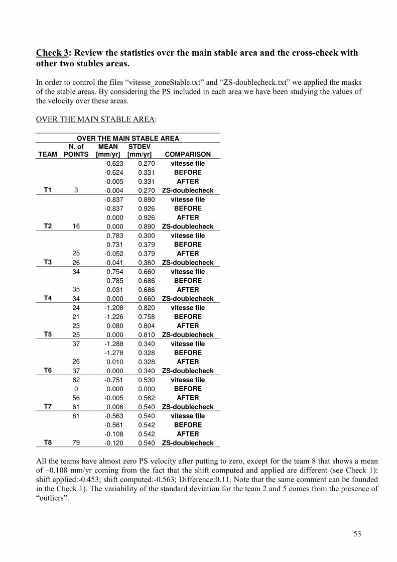
Check 3: Review the statistics over the main stable area and the cross-check with
other two stables areas. In order to control the files “vitesse_zoneStable.txt” and “ZS-doublecheck.txt” we applied the masks of the stable areas. By considering the PS included in each area we have been studying the values of the velocity over these areas. OVER THE MAIN STABLE AREA:
OVER THE MAIN STABLE AREA
TEAM N. of
POINTS MEAN
[mm/yr] STDEV [mm/yr] COMPARISON
-0.623 0.270 vitesse file
-0.624 0.331 BEFORE
-0.005 0.331 AFTER
T1 3 -0.004 0.270 ZS-doublecheck
-0.837 0.890 vitesse file
-0.837 0.926 BEFORE
0.000 0.926 AFTER
T2 16 0.000 0.890 ZS-doublecheck
0.783 0.300 vitesse file
0.731 0.379 BEFORE
25 -0.052 0.379 AFTER
T3 26 -0.041 0.360 ZS-doublecheck
34 0.754 0.660 vitesse file
0.785 0.686 BEFORE
35 0.031 0.686 AFTER
T4 34 0.000 0.660 ZS-doublecheck
24 -1.208 0.820 vitesse file
21 -1.226 0.758 BEFORE
23 0.080 0.804 AFTER
T5 25 0.000 0.810 ZS-doublecheck
37 -1.288 0.340 vitesse file
-1.278 0.328 BEFORE
26 0.010 0.328 AFTER
T6 37 0.000 0.340 ZS-doublecheck
62 -0.751 0.530 vitesse file
0 0.000 0.000 BEFORE
56 -0.005 0.562 AFTER
T7 61 0.006 0.540 ZS-doublecheck
81 -0.563 0.540 vitesse file
-0.561 0.542 BEFORE
-0.108 0.542 AFTER
T8 79 -0.120 0.540 ZS-doublecheck
All the teams have almost zero PS velocity after putting to zero, except for the team 8 that shows a mean of –0.108 mm/yr coming from the fact that the shift computed and applied are different (see Check 1): shift applied:-0.453; shift computed:-0.563; Difference:0.11. Note that the same comment can be founded in the Check 1). The variability of the standard deviation for the team 2 and 5 comes from the presence of “outliers”.
54
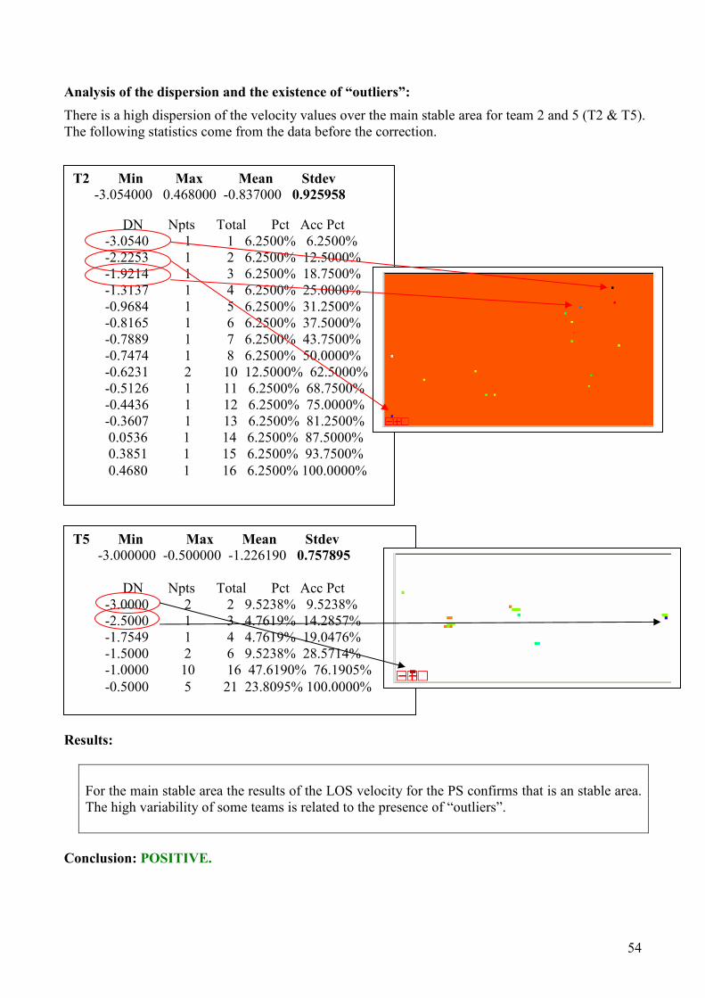
Analysis of the dispersion and the existence of “outliers”:
There is a high dispersion of the velocity values over the main stable area for team 2 and 5 (T2 & T5). The following statistics come from the data before the correction.
Results:
For the main stable area the results of the LOS velocity for the PS confirms that is an stable area. The high variability of some teams is related to the presence of “outliers”.
Conclusion: POSITIVE.
T2 Min Max Mean Stdev
-3.054000 0.468000 -0.837000 0.925958 DN Npts Total Pct Acc Pct -3.0540 1 1 6.2500% 6.2500% -2.2253 1 2 6.2500% 12.5000% -1.9214 1 3 6.2500% 18.7500% -1.3137 1 4 6.2500% 25.0000% -0.9684 1 5 6.2500% 31.2500% -0.8165 1 6 6.2500% 37.5000% -0.7889 1 7 6.2500% 43.7500% -0.7474 1 8 6.2500% 50.0000% -0.6231 2 10 12.5000% 62.5000% -0.5126 1 11 6.2500% 68.7500% -0.4436 1 12 6.2500% 75.0000% -0.3607 1 13 6.2500% 81.2500% 0.0536 1 14 6.2500% 87.5000% 0.3851 1 15 6.2500% 93.7500% 0.4680 1 16 6.2500% 100.0000%
T5 Min Max Mean Stdev -3.000000 -0.500000 -1.226190 0.757895 DN Npts Total Pct Acc Pct -3.0000 2 2 9.5238% 9.5238% -2.5000 1 3 4.7619% 14.2857% -1.7549 1 4 4.7619% 19.0476% -1.5000 2 6 9.5238% 28.5714% -1.0000 10 16 47.6190% 76.1905% -0.5000 5 21 23.8095% 100.0000%

55
OVER THE SNCF AND CIME STABLE AREAS (Cross-check of the stable area): The objective here was to analyse the velocity maps over the additional stable areas. We expected almost zero velocity values over the stable areas of SNCF or CIME. Below we show the statistics for these additional areas.
STATS SNCF
TEAM N. of
POINTS MEAN
[mm/yr] STDEV [mm/yr] COMPARISON
2 0.654 0.034 AFTER
T1 2 0.654 0.024 ZS-doublecheck
10 0.918 1.482 AFTER
T2 10 0.910 1.400 ZS-doublecheck
5 0.080 0.693 AFTER
T3 6 0.060 0.560 ZS-doublecheck
12 0.704 0.439 AFTER
T4 11 0.630 0.350 ZS-doublecheck
6 -1.675 4.248 AFTER
T5 7 -1.510 3.610 ZS-doublecheck
3 0.033 0.118 AFTER
T6 3 0.030 0.090 ZS-doublecheck
11 0.652 0.575 AFTER
T7 11 0.650 0.540 ZS-doublecheck
64 0.788 0.746 AFTER
T8 61 0.790 0.740 ZS-doublecheck
T2 Min Max Mean Stdev -1.639000 3.270000 0.917900 1.482399 DN Npts Total Pct Acc Pct -1.6390 1 1 10.0000% 10.0000% 0.1128 2 3 20.0000% 30.0000% 0.2091 1 4 10.0000% 40.0000% 0.3053 1 5 10.0000% 50.0000% 0.7481 1 6 10.0000% 60.0000% 0.9406 1 7 10.0000% 70.0000% 2.1342 1 8 10.0000% 80.0000% 2.9235 1 9 10.0000% 90.0000% 3.2700 1 10 10.0000% 100.0000%

56
Results:
In the additional stable areas, and in particular in SNCF, occurs the same of the main stable area: the presence of outliers explains the high dispersion for some results.
Conclusion: POSITIVE.
T5 Min Max Mean Stdev -10.300000 0.700000 -1.675000 4.247794 DN Npts Total Pct Acc Pct -10.3000 1 1 16.6667% 16.6667% -0.5510 1 2 16.6667% 33.3333% -0.3353 1 3 16.6667% 50.0000% 0.1824 2 5 33.3333% 83.3333% 0.7000 1 6 16.6667% 100.0000%
57
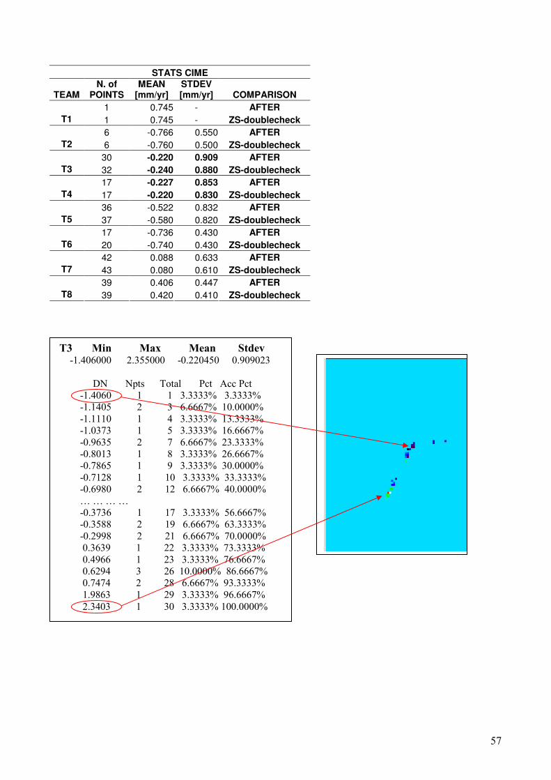
STATS CIME
TEAM N. of
POINTS MEAN
[mm/yr] STDEV [mm/yr] COMPARISON
1 0.745 - AFTER
T1 1 0.745 - ZS-doublecheck
6 -0.766 0.550 AFTER
T2 6 -0.760 0.500 ZS-doublecheck
30 -0.220 0.909 AFTER
T3 32 -0.240 0.880 ZS-doublecheck
17 -0.227 0.853 AFTER
T4 17 -0.220 0.830 ZS-doublecheck
36 -0.522 0.832 AFTER
T5 37 -0.580 0.820 ZS-doublecheck
17 -0.736 0.430 AFTER
T6 20 -0.740 0.430 ZS-doublecheck
42 0.088 0.633 AFTER
T7 43 0.080 0.610 ZS-doublecheck
39 0.406 0.447 AFTER
T8 39 0.420 0.410 ZS-doublecheck
T3 Min Max Mean Stdev -1.406000 2.355000 -0.220450 0.909023 DN Npts Total Pct Acc Pct -1.4060 1 1 3.3333% 3.3333% -1.1405 2 3 6.6667% 10.0000% -1.1110 1 4 3.3333% 13.3333% -1.0373 1 5 3.3333% 16.6667% -0.9635 2 7 6.6667% 23.3333% -0.8013 1 8 3.3333% 26.6667% -0.7865 1 9 3.3333% 30.0000% -0.7128 1 10 3.3333% 33.3333% -0.6980 2 12 6.6667% 40.0000% … … … … -0.3736 1 17 3.3333% 56.6667% -0.3588 2 19 6.6667% 63.3333% -0.2998 2 21 6.6667% 70.0000% 0.3639 1 22 3.3333% 73.3333% 0.4966 1 23 3.3333% 76.6667% 0.6294 3 26 10.0000% 86.6667% 0.7474 2 28 6.6667% 93.3333% 1.9863 1 29 3.3333% 96.6667% 2.3403 1 30 3.3333% 100.0000%

58
Results:
In the additional stable areas, and in particular in CIME, occurs the same of the main stable area: the presence of outliers explains the high dispersion for some results.
Conclusion: POSITIVE.
T4 Min Max Mean Stdev -1.524000 1.786000 -0.226941 0.853154 DN Npts Total Pct Acc Pct -1.5240 1 1 5.8824% 5.8824% -1.1346 1 2 5.8824% 11.7647% -1.1216 1 3 5.8824% 17.6471% -0.9918 1 4 5.8824% 23.5294% -0.8231 1 5 5.8824% 29.4118% -0.6933 1 6 5.8824% 35.2941% -0.4336 2 8 11.7647% 47.0588% -0.3168 1 9 5.8824% 52.9412% -0.3038 1 10 5.8824% 58.8235% -0.1740 1 11 5.8824% 64.7059% -0.0702 1 12 5.8824% 70.5882% 0.0207 1 13 5.8824% 76.4706% 0.5009 1 14 5.8824% 82.3529% 0.7735 1 15 5.8824% 88.2353% 0.9682 1 16 5.8824% 94.1176% 1.7860 1 17 5.8824% 100.0000%

59
TASK 9.2.5 REVIEW THE SPATIAL RESAMPLING OF PS DATA
• WP Leader: IG • Key Personnel: M. Crosetto, M. Agudo. • Introduction:
The objective of this task is to check the procedure used to spatially resample the PS data, and analyse the intermediate results generated by this task. This check includes two controls: a formal check of the files used in the PSIC4 Task 7.1.2; and a check of the procedure used to spatial resample the PS data.
Check 1 : The levelling coordinates used in the spatial interpolation compared
with the BRGM coordinates The BRGM and TNO files (Dataini_33800.xls and spatial_interpolation.zip, respectively) contain in principle the same coordinates for the levelling points.
In order to control the levelling coordinates used in the spatial interpolation, a comparison with the BRGM files that contain the levelling coordinates has been realized. Methodology :
See sub-task 9.2.2.1 “Check the levelling data”, Check 2. Results:
No differences between the two files. Consistency satisfactory between the input and the output.
Conclusion: POSITIVE.

60
Check 2 : Check the procedure Methodology:
The objective of Check 2 is to control the outcome of the spatial resampling procedure. For this purpose, the deformation time series of the spatially interpolated PS and the time series of the original PS have been compared, checking the agreement between them. Results:
The similar behaviour of the PS generated by the method of the spatial resampling and the original PS confirms the correctness of the resampling procedure.
Conclusion: POSITIVE.
Details of the analysis check:
In the following it is shown the scheme of the procedure used for spatial resampling of the PS data.
Levelling point
PS
Levelling point
PS

61
The following Figure shows an example of the comparison between the deformation time series of the spatially interpolated PS (bold purple line) and the time series of the original PS (different thin purple lines). This example, coming from TNO, concerns the AXE levelling line - Point: 2-2010-2.
In the above graph, which refers to the team 8, is shown the time series of the PS spatially resampled at the position of the levelling reference point (bold purple line). The thin lines correspond to the temporal evolution of the PS that are located within 50 m from the above mentioned levelling point.
In the bottom left of the above Figure are indicated the number of PS used for the spatial resampling (eight), the average distance of these PS to the position of the levelling point (40 m) and the average coherence, which represents the quality index of the PS (0.57). In this example one may notice a the good agreement (i.e. a similar same behaviour) between the resampled PS and the eight original PS. In addition, in the bottom centre of the image, is indicated a classification of the analysed PS, which is based on the type of movement (linear or non-linear) and the type of the magnitude of the movement (flat or steep). In this case, it is a steep and non-linear movement.
62
TASK 9.2.6 REVIEW THE TEMPORAL RESAMPLING OF LEVELLING
DATA
• WP Leader: IG • Key Personnel: M. Crosetto, M. Agudo. • Introduction:
The objective of this task is the check of the procedure used to temporal resample the levelling data, and analyse the intermediate results generated by this task. Furthermore, an additional check on the temporal interpolation is described in the T9.3.1 “Check and analysis of the Time Series Validation”.
Methodology:
The objective of this task is to check the procedure of the temporal resampling. This has been achieved by comparing the original levelling data with the levelling data interpolated at the dates of acquisition of the SAR images. Results:
The good agreement between the two types of information confirms the correctness of the temporal resampling procedure.
Conclusion: POSITIVE.
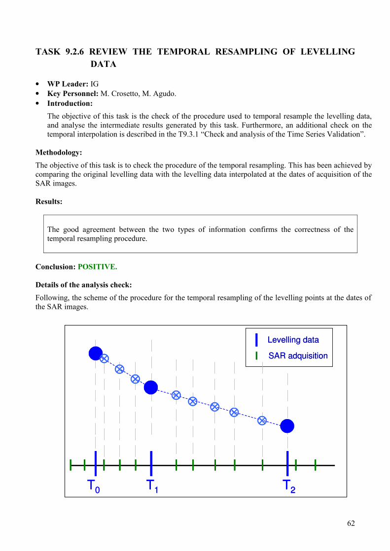
Details of the analysis check:
Following, the scheme of the procedure for the temporal resampling of the levelling points at the dates of the SAR images.
T0 T1 T2
SAR adquisition
Levelling data
T0 T1 T2T1 T2
SAR adquisition
Levelling data

63
The following figure shows an example related to the AXE levelling line, Point: RNGF_7. This graph shows the original levelling data (in pink squares) and the temporal resampling of these data, which are interpolated at the dates of the SAR images acquisitions (the interpolated values are indicated by blue dots). One may notice a good agreement between the interpolated and the original levelling data. In addition, in the next figure, at the end of the page, it is shown the kriging error of the temporal resampling for the RNGF_7 point.
Temporal resampling / versus original levelling data
Line: AXE, point: RNGF_7
-200
-150
-100
-50
0
50
01/0
1/9
2
31/1
2/9
2
01/0
1/9
4
01/0
1/9
5
02/0
1/9
6
02/0
1/9
7
02/0
1/9
8
03/0
1/9
9
03/0
1/0
0
03/0
1/0
1
04/0
1/0
2
04/0
1/0
3
05/0
1/0
4
04/0
1/0
5
05/0
1/0
6Time
Cu
mu
l d
isp
lacem
en
t (m
m) Original Levelling Data
Temporal Resampling
Kriging error
Line: AXE, point: RNGF_7
0
5
10
01/0
1/9
2
31/1
2/9
2
01/0
1/9
4
01/0
1/9
5
02/0
1/9
6
02/0
1/9
7
02/0
1/9
8
03/0
1/9
9
03/0
1/0
0
03/0
1/0
1
04/0
1/0
2
04/0
1/0
3
05/0
1/0
4
04/0
1/0
5
05/0
1/0
6
Time
Kriging error for the temporal Resampling

64
TASK 9.3 REVIEW THE VALIDATION ACTIVITIES
• WP Leader: IG • Key Personnel: M. Crosetto, M. Agudo. • Description:
This Task includes two sub-tasks:
■ T9.3.1 Check and analysis of the Time Series Validation
■ T9.3.2 Check the Velocity validation.

65
TASK 9.3.1 CHECK AND ANALYSIS OF THE TIME SERIES VALIDATION
• WP Leader: IG • Key Personnel: M. Crosetto, M. Agudo. • Introduction:
The Task 7.2.2.1 “Time Series Validation” of PSIC4 represents one of the most important steps in the entire validation activities. In this task some analyses and interpretations have been performed on the time series.
Methodology:
In this task the levelling and the PS data have been compared. This was performed by analysing the time series graphs provided by TNO.
In addition, it is worth to underline that in the Task 10 of PSIC4 a detail analysis of the time series has been performed, by comparing the levelling data with the DInSAR data. The good agreement between them confirms the correctness of the time series. Results:
During the analyses and interpretations performed on the time series the correctness of the time series has been confirmed.
Conclusion: POSITIVE.
Comments:
In the Annex 5 of this document, are shown different graphs relative to several levelling lines. In each graph is shown the temporal evolution of the levelling point (in black) and the temporal evolution of the resampled PS. Each graph contains the data of at least one or several teams. Using these graphs some analyses and interpretations of the time series have been performed. The outcomes of these analyses are briefly summarized in the following page.
One example is illustrated in the Figure of the following page. For this Figure is provided the same information that is given for the graph analysed in the Check 2 of task 9.2.5: in the bottom left of the image are indicated the number of PS used for the spatial resampling, the average distance of these PS to the position of the levelling point, and the average coherence. In addition, in the bottom centre of the image is indicated the classification of the type of movement (linear or non-linear) and the type of the magnitude of the movement (flat or steep). In this case is a steep and non-linear movement.
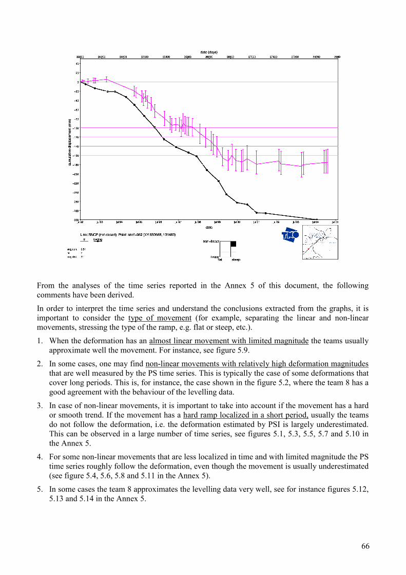
66
From the analyses of the time series reported in the Annex 5 of this document, the following comments have been derived.
In order to interpret the time series and understand the conclusions extracted from the graphs, it is important to consider the type of movement (for example, separating the linear and non-linear movements, stressing the type of the ramp, e.g. flat or steep, etc.).
1. When the deformation has an almost linear movement with limited magnitude the teams usually approximate well the movement. For instance, see figure 5.9.
2. In some cases, one may find non-linear movements with relatively high deformation magnitudes that are well measured by the PS time series. This is typically the case of some deformations that cover long periods. This is, for instance, the case shown in the figure 5.2, where the team 8 has a good agreement with the behaviour of the levelling data.
3. In case of non-linear movements, it is important to take into account if the movement has a hard or smooth trend. If the movement has a hard ramp localized in a short period, usually the teams do not follow the deformation, i.e. the deformation estimated by PSI is largely underestimated. This can be observed in a large number of time series, see figures 5.1, 5.3, 5.5, 5.7 and 5.10 in the Annex 5.
4. For some non-linear movements that are less localized in time and with limited magnitude the PS time series roughly follow the deformation, even though the movement is usually underestimated (see figure 5.4, 5.6, 5.8 and 5.11 in the Annex 5).
5. In some cases the team 8 approximates the levelling data very well, see for instance figures 5.12, 5.13 and 5.14 in the Annex 5.
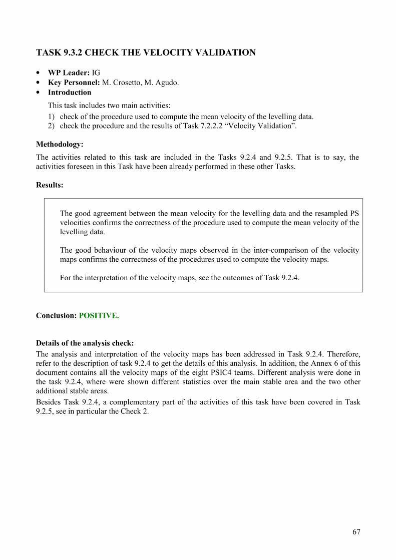
67
TASK 9.3.2 CHECK THE VELOCITY VALIDATION
• WP Leader: IG • Key Personnel: M. Crosetto, M. Agudo. • Introduction
This task includes two main activities:
1) check of the procedure used to compute the mean velocity of the levelling data. 2) check the procedure and the results of Task 7.2.2.2 “Velocity Validation”.
Methodology:
The activities related to this task are included in the Tasks 9.2.4 and 9.2.5. That is to say, the activities foreseen in this Task have been already performed in these other Tasks. Results:
The good agreement between the mean velocity for the levelling data and the resampled PS
velocities confirms the correctness of the procedure used to compute the mean velocity of the levelling data.
The good behaviour of the velocity maps observed in the inter-comparison of the velocity
maps confirms the correctness of the procedures used to compute the velocity maps. For the interpretation of the velocity maps, see the outcomes of Task 9.2.4.
Conclusion: POSITIVE.
Details of the analysis check:
The analysis and interpretation of the velocity maps has been addressed in Task 9.2.4. Therefore, refer to the description of task 9.2.4 to get the details of this analysis. In addition, the Annex 6 of this document contains all the velocity maps of the eight PSIC4 teams. Different analysis were done in the task 9.2.4, where were shown different statistics over the main stable area and the two other additional stable areas.
Besides Task 9.2.4, a complementary part of the activities of this task have been covered in Task 9.2.5, see in particular the Check 2.

68
TASK 9.4 REVIEW THE INTER-COMPARISON ACTIVITIES
• WP Leader: IG • Key Personnel: M. Crosetto, M. Agudo. • Description:
This Task includes two sub-tasks:
■ T9.4.1 Check the estimation of PS spatial distribution and densities
■ T9.4.2 Check the Inter-comparison of velocity maps
■ T9.4.3 Check the APS inter-comparison
■ T9.4.4 Check of the geocoding inter-comparison.

69
TASK 9.4.1 CHECK THE ESTIMATION OF PS SPATIAL DISTRIBUTION
AND DENSITIES
• WP Leader: IG • Key Personnel: M. Crosetto, M. Agudo. • Introduction
This task involves a generic check of the PSIC4 Task 7.3.1 “PSI spatial distribution and densities”. Methodology:
The key activities related to this task have been performed in the frame of Task 9.2.4. Results:
The distribution and densities of the PS have been analysed in the Task 9.2.4.
Conclusion: POSITIVE.
Details of the analysis check:
See task 9.2.4 and Annex 6 of this document to get more information about the data contained in the velocity maps, the different densities and the distribution of each team.
Comments:
1. Using the visualization of the velocities maps the different densities of the teams have been analysed. The teams 7 and 8 have the higher density. Note that for the team 8 the correction of the geocoding was impossible due to a high density and a spatial distribution of the PS over the orthoimage (the density does not match with urban features, etc.).
2. Due to the fact that the teams used different cut-off values to define their PS, different PS densities and spatial distributions are obtained. In addition, the shape of the spatial distribution is related to the land cover of the studied area. For example, in urban areas the coherence is better and, then, a higher number of PS is obtained, while the number decreases in forest areas where the coherence is minor.

70
TASK 9.4.2 CHECK THE INTER-COMPARISON OF VELOCITY MAPS
• WP Leader: IG • Key Personnel: M. Crosetto, M. Agudo. • Introduction:
This task involves a generic check of the Task 7.3.4 “Inter-comparison of velocity maps”. The activities related to this task have been performed in the frame of Task 9.2.4. In this task, in fact, the mean and standard deviation of the velocities have been computed over two types of areas:
a) the main stable area and the two other stable areas,
b) different deformation areas.
This check was entirely included in the task 9.2.4, where the velocity maps have been analysed. By computing the statistics over the stable and not stable areas different patterns in the velocity maps have been found. Furthermore, with by visualizing the velocity maps different densities have been founded for each team, as it has been already mentioned in the task 9.4.1.
Results:
The good inter-comparison between the velocity maps of the teams confirms the correctness of the procedure used to derive the velocity maps.
Conclusion: POSITIVE.
Details of the analysis check:
See the description of Task 9.2.4 for the analysis of the velocity maps of each team. Furthermore, the Annex 6 contains the velocity maps of the PSIC4 teams.

71
TASK 9.4.3 CHECK THE APS INTER-COMPARISON
• WP Leader: IG • Key Personnel: M. Crosetto, M. Agudo. • Introduction:
This task involves a generic check of the Task 7.3.2 “APS Inter-comparison”. Its objective is to analyse the APS maps, by comparing them with the velocity maps in order to detect any correlation between them. The goal of this analysis is to highlight potential artefacts in the APS related to the deformation areas.
Results:
There are no evident APS patterns related to the velocity maps, with the exception of the teams 1 and 3.
Conclusion: POSITIVE.
Details of the analysis check:
In the following, the APS estimated by each team for the image 33835 (19/08/1992), is analysed in detail.
■ Team 1. The velocity and the APS map show the same spatial pattern. This means that the estimation of the APS is probably affected by a contribution due to the terrain deformation. This clearly represents an error of the estimation process (see Figure 4.3.1).
Figure 4.3.1. On the left, the velocity map of the team 1. On the right, its APS map.

72
■ Team 2. No pattern related to the deformation has been found (see Figure 4.3.2).
Figure 4.3.2. On the left, the velocity map of the team 2. On the right, its APS map.
■ Team 3. More or less the same pattern of team 1 has been found. The highest values for the APS
are localized in the deformation area, i.e. in the centre of the image (see Figure 4.3.3).
Figure 4.3.3. On the left, the velocity map of the team 3. On the right, its APS map.
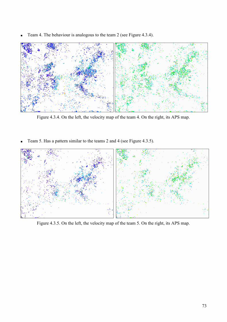
73
■ Team 4. The behaviour is analogous to the team 2 (see Figure 4.3.4).
Figure 4.3.4. On the left, the velocity map of the team 4. On the right, its APS map. ■ Team 5. Has a pattern similar to the teams 2 and 4 (see Figure 4.3.5).
Figure 4.3.5. On the left, the velocity map of the team 5. On the right, its APS map.
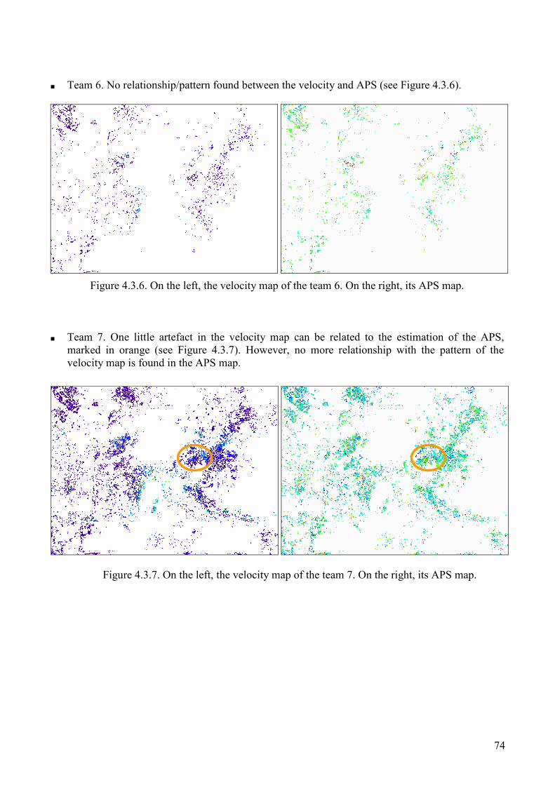
74
■ Team 6. No relationship/pattern found between the velocity and APS (see Figure 4.3.6).
Figure 4.3.6. On the left, the velocity map of the team 6. On the right, its APS map. ■ Team 7. One little artefact in the velocity map can be related to the estimation of the APS,
marked in orange (see Figure 4.3.7). However, no more relationship with the pattern of the velocity map is found in the APS map.
Figure 4.3.7. On the left, the velocity map of the team 7. On the right, its APS map.
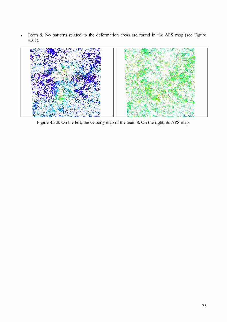
75
■ Team 8. No patterns related to the deformation areas are found in the APS map (see Figure
4.3.8).
Figure 4.3.8. On the left, the velocity map of the team 8. On the right, its APS map.

76
TASK 9.4.4 CHECK OF THE GEOCODING INTER-COMPARISON
• WP Leader: IG • Key Personnel: M. Crosetto, M. Agudo. • Introduction
This task involves a generic check of the PSIC4 Task 7.3.3 “Geocoding inter-comparison”. Results:
The outcomes of the Task 7.3.3, i.e. the average geocoding differences and the standard deviations of the geocoding differences, only provide a rough information on the geocoding inter-comparison.
Conclusion: POSITIVE, however one has to take into account that the statistics derived in this task only provide rough estimation values to inter-compare the geocoding of the different teams.
Details of the analysis check:
The procedure used in Task 7.3.3, “Geocoding inter-comparison”, allows a large number of pairs of radar targets to be selected. However, this procedure only provides a rough estimation of the geocoding shifts between pairs of PSIC4 teams. In fact, it does not consider that the teams adopt different reference systems in the radar space, i.e. that the radar images used by the different teams are not perfectly co-registered. For this reason it is suggested to consider this limitation of the adopted procedure when analysing the results of Task 7.3.3.

77
CONCLUSIONS
The Task 9 of the PSIC4 project has been devoted to a comprehensive check of all the data processing and analysis tasks preformed by the PSIC4 validation team in order to validate and inter-compare the PSI results. The comprehensive check has been focused on two key components of the PSIC4 project:
- the levelling data, that are in situ data used as reference for the validation,
- the methods and procedures used for the validation and inter-comparison tasks.
The comprehensive check has given positive results for all the tasks and sub-tasks of Task 9. Few exceptions concern some validation and inter-comparison sub-tasks. These exceptions, which are documented in detail in this report, have negligible influence on the PSIC4 validation results.
The cross-check of the levelling data has been mainly based on extra information provided by Carbonnage de France. By analysing those levelling traverses that have estimated closing errors (closed traverses) the good global quality of the levelling data has been highlighted.
The cross-check of all the validation and inter-comparison tasks has required a remarkable exchange of intermediate results between the PSIC4 validation teams. This cross-check has been based on different complementary approaches:
1. Collecting extra data, e.g. those provided by Carbonnage de France to check a key validation feature: the correct planimetric positioning of the levelling data.
2. Performing simple formal checks on the inputs and outputs of the different tasks and sub-tasks.
3. Designing ad hoc checks, specifically conceived for checking and verification purposes. For instance, some of these checks have been performed to get independent computations, by using independent software, from those performed by the PSIC4 validation team.
4. An important type of cross-checks has been implicitly performed by be analysing different aspects of the same type of data, e.g. see the different validation and inter-comparison activities that are related to the velocity maps.
Again, the different cross-checks have globally provided positive results. Therefore the outcomes of the validation and inter-comparison results have shown to be consistent and reliable: they represent a technically sound base to be used to assess the PSI performances over the Gardanne test site.