PSSE Redux: Convex Relaxation, Decentralized,

Robust, and Dynamic Approaches

Vassilis Kekatos, Gang Wang, Hao Zhu, and Georgios B. Giannakis ∗

August 15, 2017

1 Introduction

With the advent of digital computers, power system engineers in the 1960stried computing the voltages at critical buses based on readings from cur-rent and potential transformers. Local personnel manually collected thesereadings and forwarded them by phone to a control center. Nevertheless,due to timing, modeling, and instrumentation inaccuracies, the power flowequations were always infeasible. In a seminal contribution [61], the statisti-cal foundations were laid for a multitude of grid monitoring tasks, includingtopology detection, static state estimation, exact and linearized models, baddata analysis, centralized and decentralized implementations, as well as dy-namic state tracking. Since then, different chapters, books, and review arti-cles have nicely outlined the progress in the area; see for example [74, 55, 1].The revolutionary monitoring capabilities enabled by synchrophasor unitshave been put forth in [58].

This chapter aspires to glean some of the recent advances in power sys-tem state estimation (PSSE), though our collection is not exhaustive byany means. The Cramer-Rao bound, a lower bound on the (co)variance

∗V. Kekatos is with the Bradley Department of Electrical and Computer Engineering,Virginia Tech, Blacksburg, VA 24061, USA. G. Wang is with the Department of Electri-cal and Computer Engineering, University of Minnesota, Minneapolis, MN 55455, USA,and also with the State Key Lab of Intelligent Control and Decision of Complex Sys-tems, Beijing Institute of Technology, Beijing 100081, P. R. China. H. Zhu is with theDepartment of Electrical and Computer Engineering, University of Illinois, Urbana, IL61801. G. B. Giannakis is with the Department of Electrical and Computer Engineer-ing, University of Minnesota, Minneapolis, MN 55455, USA. E-mails: kekatos@vt.edu;{gangwang, georgios}@umn.edu; haozhu@illinois.edu.

1

arX

iv:1

708.

0398

1v1

[cs

.SY

] 1

4 A

ug 2

017

of any unbiased estimator, is first derived for the PSSE setup. After re-viewing the classical Gauss-Newton iterations, contemporary PSSE solversleveraging relaxations to convex programs and successive convex approxima-tions are explored. A disciplined paradigm for distributed and decentralizedschemes is subsequently exemplified under linear(ized) and exact grid mod-els. Novel bad data processing models and fresh perspectives linking criticalmeasurements to cyber-attacks on the state estimator are presented. Fi-nally, spurred by advances in online convex optimization, model-free andmodel-based state trackers are reviewed.

Notation: Lower- (upper-) case boldface letters denote column vec-tors (matrices), and calligraphic letters stand for sets. Vectors 0, 1, anden denote respectively the all-zero, all-one, and the n-th canonical vectorsof suitable dimensions. The conjugate of a complex-valued object (scalar,vector or matrix) x is denoted by x∗; <{x} and ={x} are its real and imag-inary parts, and j :=

√−1. Superscripts T and H stand for transpose and

conjugate-transpose, respectively, while Tr(X) is the trace of matrix X. Adiagonal matrix having vector x on its main diagonal is denoted by dg(x);whereas, the vector of diagonal entries of X is dg(X). The range space of Xis denoted by range(X); and its null space (kernel) by null(X). The notationN (µ,Σ) represents the Gaussian distribution with mean µ and covariancematrix Σ.

2 Power Grid Modeling

This section introduces notation and briefly reviews the power flow equa-tions; for detailed exposition see e.g., [1], [19] and references therein. Apower system can be represented by the graph G = (B,L), where the nodeset B comprises its Nb buses, and the edge set L its Nl transmission lines.Given the focus on alternating current (AC) power systems, steady-statevoltages and currents are represented by their single-phase equivalent pha-sors per unit.

A transmission line (n, k) ∈ L running across buses n, k ∈ B is modeledby its total series admittance ynk = gnk + jbnk, and total shunt susceptancejbsnk. If Vn is the complex voltage at bus n, the current Ink flowing frombus m to bus n over line (m,n) is

Ink = (ynk + jbsnk/2)Vn − ynkVn. (1)

The current Inm coming from the other end of the line can be expressedsymmetrically. That is not the case if the two buses are connected via a

2

transformer with complex ratio ρnk followed by a line, where

Ink =ynk + jbsnk/2

|ρnk|2Vn −

ynkρ∗nkVn (2a)

Inm = (ynk + jbsnk/2)Vn −ynkρnkVn. (2b)

Kirchhoff’s current law dictates that the current injected into bus n isIn =

∑n∈Bn Ink, where Bn denotes the set of buses directly connected to

bus n. If vector i ∈ CNb collects all nodal currents, and v ∈ CNb all nodalvoltages, the two vectors are linearly related through the bus admittancematrix Y = G + jB as

i = Yv. (3)

Similar to (3), line currents can be stacked in the 2Nl-dimensional vector if ,and expressed as a linear function of nodal voltages

if = Yfv (4)

for some properly defined 2Nl ×Nb complex matrix Yf [cf. (1)–(2)].The complex power injected into bus n will be denoted by Sn := Pn +

jQn. Since by definition Sn = VnI∗n, the vector of complex power injectionss = p + jq can be expressed as

s = dg(v)i∗ = dg(v)Y∗v∗. (5)

The power flowing from bus n to bus n over line (m,n) is Snk = VnI∗nk.If voltages are expressed in polar form Vn = Vne

jθn , the power flowequations in (5) per real and imaginary entry can be written as

Pn =

Nb∑n=1

VnVn [Gnk cos(θn − θn) +Bnk sin(θn − θn)] (6a)

Qn =

Nb∑n=1

VnVn [Gnk sin(θn − θn)−Bnk cos(θn − θn)] . (6b)

Since power injections are invariant if voltages are shifted by a commonangle, the voltage phase is arbitrarily set to zero at a particular bus calledthe reference bus.

Alternatively to (6), if voltages are expressed in rectangular coordinatesVn = Vr,m + jVi,m, power injections are quadratically related to voltages

Pn = Vr,m

Nb∑n=1

(Vr,nGnk − Vi,nBnk) + Vi,m

Nb∑n=1

(Vi,nGnk + Vr,nBnk) (7a)

3

Qn = Vi,m

Nb∑n=1

(Vr,nGnk − Vi,nBnk)− Vr,mNb∑n=1

(Vi,nGnk + Vr,nBnk). (7b)

To compactly express (7), observe that S∗n = V∗nIn = (vHen)(eTn i) =vHene

TnYv from which it readily follows that

Pn = vHHPnv (8a)

Qn = vHHQnv (8b)

where the involved matrices are defined as

HPn :=1

2

(ene

TnY + YHene

Tn

)(9a)

HQn :=1

2j

(ene

TnY −YHene

Tn

). (9b)

Similar expressions hold for the squared voltage magnitude at bus n:

V 2n = vHHVnv, where HVn := ene

Tn . (10)

Realizing that a line current can also be provided as Ink = eTnkif , thepower flow on line (n, k) as seen from bus n is expressed as S∗nk = V∗nInk =(vHen)(eTnkif ) = vHene

TnkYfv, from which it follows that

Pnk = vHHPnkv (11a)

Qnk = vHHQnkv (11b)

where HPnkand HQnk

are defined by substituting eTnY and YHen by eTnkYf

and YHf enk in (9), accordingly.Equations (8), (10) and (11) explain how power injections, flows, and

squared voltage magnitudes are quadratic functions of voltage phasors asdescribed by vHHmv for certain complex Nb×Nb matrices Hm. Regardlessif Y and/or Yf are symmetric or Hermitian, Hm are Hermitian by definition.This means that Hm = HHm, or equivalently, <{Hm}T = <{Hm}, and={Hm}T = −={Hm}. It can be easily verified that the quadratic functionscan be expressed in terms of real-valued quantities as

vHHmv = vT Hmv (12)

for the expanded real-valued voltage vector v := [<{v}T ={v}T ]T , and thereal-valued counterpart of Hm, namely

Hm :=

[<{Hm} −={Hm}={Hm} <{Hm}

]. (13)

4

3 Problem Statement

It was seen in Section 2 that given grid parameters collected in Y and Yf , allpower system quantities can be expressed in terms of the voltage vector v,which justifies its term as the system state. Meters installed across the gridmeasure electric quantities, and forward their readings via remote terminalunits to a control center for grid monitoring. Due to lack of synchronization,conventional meters cannot utilize the angle information of phasorial quan-tities. For this reason, legacy measurements involve phaseless power injec-tions and flows along with voltage and current magnitudes at specific buses.The advent of the global positioning system (GPS) facilitated a precise tim-ing signal across large geographical areas, thus enabling the revolutionarytechnology of synchrophasors or phasor measurement units (PMUs) [58].Recovering bus voltages given network parameters and the available mea-surements constitutes the critical task of power system state estimation.This section formally states the problem, provides the Cramer-Rao boundon the variance of any unbiased estimator, and reviews the Gauss-Newtoniterations. Solvers based on semidefinite relaxation and successive convexapproximations are subsequently explicated, and the section is wrapped upwith issues germane to PMUs.

3.1 Weighted Least-Squares Formulation

Consider M real-valued measurements {zm}Mm=1 related to the complexpower system state v through the model

zm = hm(v) + εm (14)

where hm(v) : CNb → R is a (non)-linear function of v, and εm capturesthe measurement noise and modeling inaccuracies. Collecting measurementsand noise terms in vectors z and ε accordingly, the vector form of (14) reads

z = h(v) + ε (15)

for the mapping h : CNb → RM . Model (15) is instantiated for differenttypes of measurements next.

Traditionally, the system state v is expressed in polar coordinates, namelynodal voltage magnitudes and angles. Then h(v) maps the 2Nb-dimensionalstate vector to SCADA measurements through the nonlinear equations (6).Expressing the states in polar form has been employed primarily due to tworeasons. First, the Jacobian matrix of h(v) is amenable to approximations.

5

Secondly, voltage magnitude measurements are directly related to states.Nevertheless, due to recent computational reformulations, most of our ex-position models voltages in the rectangular form. Then, as detailed in (12),the m-th SCADA measurement zm involves the quadratic function of thestate hm(v) = vHHmv for a Hermitian matrix Hm.

Expressing voltages in rectangular coordinates is computationally ad-vantageous when it comes to synchrophasors too. As evidenced by (3)–(4),PMU measurements feature linear mappings hm(v). If PMU measurementsare expressed in rectangular coordinates, the model in (14) simplifies to

z = Hv + ε (16)

for an M × Nb complex matrix H, and complex-valued noise ε. Followingthe notation of (12)–(13), the linear measurement model of (16) can beexpressed in terms of real-valued quantities as

z = (H∗)v + ε. (17)

The random noise vector ε in (15) is usually assumed independent ofh(v), zero-mean and circularly symmetric, that is E[εεH] = Σε and E[εεT ] =0. The last assumption holds if for example the real and imaginary compo-nents of ε are independent and have identical covariance matrices. This istrue for a PMU measurement, where the actual state lies at the center of aspherically-shaped noise cloud on the complex plane.

Moreover, the entries of ε are oftentimes assumed uncorrelated yieldinga diagonal covariance Σε = dg({σ2m}) with σ2m being the variance of them-th entry εm. However, that may not always be the case. For example,active and reactive powers at the same grid location are derived as productsbetween the readings of a current transformer and a potential transformer.Further, noise terms may be correlated between the real and imaginary partsof the same phasor in a PMU.

Adopting the weighted least-squares (WLS) criterion, power system stateestimation can be formulated as

minimizev∈CNb

‖Σ−1/2ε (z− h(v))‖22 (18)

where Σ−1/2ε is the matrix square root of the inverse noise covariance matrix.

If the noise is independent across measurements, then (18) simplifies to

minimizev

M∑m=1

(zm − hm(v))2

σ2m. (19)

6

Either way, the PSSE task boils down to a (non)-linear least-squares (LS) fit.When the mapping h(v) is linear or when the entries of ε are uncorrelated,the measurement model in (15) can be prewhitened. For example, the linearmeasurement model z = Hv + ε can be equivalently transformed to

Σ−1/2ε z = (Σ−1/2ε H)v + Σ−1/2ε ε (20)

so that the associated noise Σ−1/2ε ε is now uncorrelated. To ease the presen-

tation, the noise covariance will be henceforth assumed Σε = IM , yielding

v := arg minv

M∑m=1

(zm − hm(v))2. (21)

For Gaussian measurement noise ε ∼ N (0, IM ), the minimizer of (21) coin-cides with the maximum likelihood estimate (MLE) of v [29].

3.2 Cramer-Rao Lower Bound Analysis

According to standard results in estimation theory [29], the variance ofany unbiased estimator is lower bounded by the Cramer-Rao lower bound(CRLB). Appreciating its importance as a performance benchmark acrossdifferent estimators, the ensuing result shown in the Appendix derives theCRLB for any unbiased power system state estimator based on the so-termedWirtinger’s calculus for complex analysis [41].

Proposition 1. Consider estimating the unknown state vector v ∈ CNb

from the noisy SCADA data {zm}Mm=1 of (15), where the Gaussian mea-surement error εm is independent across meters with mean zero and varianceσ2m. The covariance matrix of any unbiased estimator v satisfies

Cov(v) � [F†(v,v∗)]1:Nb,1:Nb(22)

where the Fisher information matrix (FIM) is given as

F(v,v∗)=

[ ∑Mm=1

1σ2m

(Hmv)(Hmv)H∑M

m=11σ2m

(Hmv)(H∗mv∗)H∑Mm=1

1σ2m

(H∗mv∗)(Hmv)H∑M

m=11σ2m

(H∗mv∗)(H∗mv∗)H

].

(23)In addition, matrix F(v,v∗) has at least rank-one deficiency even when allpossible SCADA measurements are available.

Although rank-deficient, the pseudo-inverse of F(v,v∗) qualifies as avalid lower bound on the mean-square error (MSE) of any unbiased estima-tor [63]. Rank deficiency of the FIM originates from the inherent voltage

7

angle ambiguity: SCADA measurements remain invariant if nodal voltagesare shifted globally by a unimodular phase constant. Fixing the angle ofthe reference bus waives this issue. It is also worth stressing that the CRLBin Prop. 1 is oftentimes attainable and benchmarks the optimal estimatorperformance [63]. Having derived the CRLB for the PSSE task, our nextsubsection deals with PSSE solvers.

3.3 Gauss-Newton Iterations

Consider for specificity model (16), though the real-valued model in (17)or the model involving polar coordinates could be employed as well. Whenthe noise covariance matrix Σε = IM , the PSSE task in (18) reduces to thenonlinear LS problem

minimizev∈CNb

‖z− h(v)‖22 (24)

for which the Gauss-Newton iterations are known to offer the “workhorse”solution [3, Ch. 1], [1, Ch. 2]. According to the Gauss-Newton method,the function h(v) is linearized at a given point vi ∈ CNb using Taylor’sexpansion as

h(v,vi) := h(vi) + Ji(v − vi)

where Ji := ∇h(vi) is the M × Nb Jacobian matrix of h evaluated at vi,whose (m,n)-th entry is given by the Wirtinger derivative ∂hm/∂Vn; seee.g., [41] for Wirtinger’s calculus. The Gauss-Newton method subsequentlyapproximates the nonlinear LS fit in (24) with a linear one of h, and relieson its minimizer to obtain the next iterate as

vi+1 ∈ arg minv

∥∥z− h(v,vi)∥∥2

= arg minv

∥∥z− h(vi)∥∥2 − 2(v − vi)H(Ji)H(z− h(vi))

+ (v − vi)H(Ji)HJi(v − vi). (25)

When matrix (Ji)HJi is invertible, vi+1 can be found in closed form as

vi+1 = vi +[(Ji)HJi

]−1(Ji)H(z− h(vi)). (26)

The state estimate is iteratively updated using (26) until some stoppingcriterion is satisfied.

If, on the other hand, the WLS cost (18) is minimized, the Gauss-Newton

iterations can be similarly obtained by treating Σ−1/2ε z as z and Σ

−1/2ε h(v)

as h(v) in (24), yielding

vi+1 = vi +[(Ji)HΣ−1ε Ji

]−1(Ji)HΣ−1ε (z− h(vi)). (27)

8

It is well known that the pure Gauss-Newton iterations in (26) or (27)may not guarantee convergence, which in fact largely depends on the startingpoint v0 [3, Ch. 1.5]. A common way to improve convergence and ensuredescent of the cost in (18) consists of including a backtracking line search in(27) to end up with

vi+1 = vi + µi[(Ji)HΣ−1ε Ji

]−1(Ji)HΣ−1ε (z− h(vi)) (28)

where the step size µi > 0 is found through the backtracking line searchrule [3, Ch. 1.2]. Due to its intimate relationship with ordinary gradient de-scent alternatives for nonconvex optimization however, this Gauss-Newtoniterative procedure can be trapped by local solutions [3, Ch. 1.5]. In anutshell, the grand challenge remains to develop PSSE solvers capable of at-taining or approximating the global optimum at manageable computationalcomplexity. A few recent proposals in this direction are presented next.

3.4 Semidefinite Relaxation

A method to tackle the nonlinear measurement model that can convert thePSSE problem of (21) to a convex semidefinite program (SDP) has beenintroduced in [83], [84]. Consider first expressing each measurement in zlinearly in terms of the outer-product matrix V := vvH. In this way, thequadratic models in (8), (10), and (11) can be transformed to linear ones interms of the matrix variable V. Thus, each noisy measurement in (14) canbe written as zm = vHHmv + εm = Tr(HmV) + εm. Rewriting the PSSEtask in (21) accordingly in terms of V reduces to

V1 := arg minV∈CNb×Nb

M∑m=1

[zm − Tr(HmV)

]2(29a)

s. to V � 0, and rank(V) = 1 (29b)

where the positive semi-definite (PSD) and the rank-1 constraints jointlyensure that for any V obeying (29b), there always exists a vector v suchthat V = vvH.

Although zm and V are linearly related as in (29), nonconvexity is stillpresent in two aspects: (i) the cost function in (29a) has degree 4 in theentries of V; and (ii) the rank constraint in (29b) is nonconvex. Aimingfor an SDP reformulation of (29), Schur’s complement lemma, see e.g., [5,Appx. 5.5], can be leveraged to tightly bound each summand in (29a) using

9

an auxiliary variable χm > 0. Collecting all χm’s in χ ∈ Rm, the problemin (29) can be expressed as

{V2, χ2} := arg minV, χ

1T χ (30a)

s. to V � 0, and rank(V) = 1 (30b)[χm zm − Tr(HmV)

zm − Tr(HmV) 1

]�0, ∀m. (30c)

The equivalence among all three SE problems (21), (29), and (30) has beenshown in [83], where their optimal solutions satisfy:

V1 = V2 = vvH, and χ2,m =[zm − Tr(HmV2)

]2, ∀m. (31)

The only source of nonconvexity in the equivalent SE problem of (30)comes from the rank-1 constraint. Motivated by the technique of semidefi-nite relaxation (SDR); see e.g., the seminal work of [21], one can obtain thefollowing convex SDP upon dropping the rank constraint

{V, χ} := arg minV, χ

1T χ (32a)

s. to V � 0, and (30c). (32b)

For the SDR-PSSE formulation in (32), a few assumptions have beenmade in [84] to establish its global optimality in a specific setup.

(as1) The graph G = (B,L) has a tree topology;

(as2) Every bus is equipped with a voltage magnitude meter; and

(as3) All measurements in z are noise-free, that is ε = 0.

Proposition 2. Under (as1)-(as3), solving the relaxed problem (32) at-tains the global optimum of the original PSSE problem (30) or (21); that is,rank(V) = 1.

Assumptions (as1)-(as3) may offer a close approximation of the realisticPSSE scenario, thanks to characteristics of transmission systems such assparse connectivity, almost flat voltage profile, and high metering accuracy.Although they do not hold precisely in realistic transmission systems, near-optimality of the relaxed problem (32) has been numerically supported byextensive tests [84]. A more crucial issue is to recover a feasible SE solutionfrom the relaxed problem (32), as V is very likely to have rank greater than1. This is possible either by finding the best rank-1 approximation to V viaeigenvalue decomposition, or via randomization [46].

10

SDR endows SE with a convex SDP formulation for which efficientschemes are available to obtain the global optimum using for example theinterior-point solver. The computational complexity for eigen-decompositionis in the order of matrix multiplication, and thus negligible compared tosolving the SDP; see [46] and references therein. However, the polynomialcomplexity of solving the SDP could be a burden for real-time power sys-tem monitoring, which motivates well the distributed implementation ofSection 4.2.

3.5 Penalized Semidefinite Relaxation

Building on an alternative formulation of the power flow problem, a penalizedversion of the aforementioned SDP-based state estimator has been devisedin [48, 47, 78]. Commencing with the power flow task, it can be interpretedas a particular instance of PSSE, where:

• Measurements (henceforth termed specifications) are noiseless;

• Excluding the reference bus, buses are partitioned into the subset BPVfor which active injections and voltage magnitudes are specified, andthe subset BPQ, for which active and reactive injections are specified.

The power flow task can be posed as the feasibility problem; that is,

find v ∈ CNb (33)

s. to Pn = vHHPnv, ∀n ∈ BPV ∪ BPQQn = vHHQnv, ∀n ∈ BPQV 2n = vHHVnv, ∀n ∈ BPV, and V 2

ref = V0.

Using the SDP reformulation presented earlier, the power flow task can beequivalently expressed as

find V ∈ CNb×Nb (34)

s. to zm = Tr(HmV), m = 1, . . . , 2Nb − 1

V � 0, and rank(V) = 1

where the specifications (constraints) of (33) have been generically capturedby the pairs {(zm; Hm)}2Nb−1

m=1 .Although the optimization in (34) is non-convex, a convex relaxation

can be obtained by dropping the rank constraint. To promote rank-onesolutions, the feasibility problem is further reduced to [48]

V := arg minV�0

Tr(H0V) (35)

11

s. to zm = Tr(HmV), m = 1, . . . , 2Nb − 1. (36)

If the Hermitian matrix H0 is selected such that H0 � 0, rank(H0) = Nb−1,and H01 = 0; then any state v close to the flat voltage profile 1 + j0 canbe recovered from the rank-one minimizer V of (35); see [48, Thm. 2]. Thestated conditions exclude the case H0 = INb

that would have led to thenuclear-norm heuristic commonly used in low-rank matrix completion.

Spurred by this observation, the PSSE task can be posed as [47]

Vµ := arg minV�0

Tr(H0V) + µM∑m=1

fm(zm − Tr(HmV)

)(37)

for some regularization parameter µ ≥ 0, where M now can be larger than2Nb− 1. The second term in the cost of (37) is a data-fitting term ensuringthat the recovered state is consistent with the collected measurements basedon selected criteria. Two cases for fm of special interest are the LS fitfLSm (ε) := ε2, and the least-absolute value (LAV) one fLAVm (ε) := |ε|, ∀m =1, . . . ,M . On the other hand, the first term in (37) can be understood as aregularizer to promote rank-one solutions Vµ; see more details in [47].

In the noiseless setup, where all measurements comply with the modelzm = vH0 Hmv0, the minimization in (37) has been shown to possess a rank-one minimizer Vµ = vµv

Hµ for all µ ≥ 0 under both fLSm and fLAVm ; see

details in [47]. Interestingly, the solution vµ obtained under the LS fit doesnot coincide with v0 for any µ ≥ 0, whereas the LAV solution vµ provides

the actual state v0 for a sufficiently large µ. Error bounds between Vµ

and v0vH0 under the regularized LAV solution for noisy measurements are

established in [78].

3.6 Feasible Point Pursuit

The feasible point pursuit (FPP) method studied in [51] offers anothercomputationally manageable solver for approximating the globally optimalPSSE. As a special case of the convex-concave procedure [44], FPP is an it-erative algorithm for handling general nonconvex quadratically constrainedquadratic programs (QCQPs) [77]. It approximates the feasible solutions ofa nonconvex QCQP by means of a sequence of convexified QCQPs obtainedwith successive convex inner-restrictions of the original nonconvex feasibilityset [77].

The first step in applying FPP to PSSE is a reformulation of (18) into

12

a standard QCQP [71, 70]

minimizev∈CNb , χ∈RM

χTΣ−1ε χ (38a)

s. to vHHmv ≤ zm + χm, 1 ≤ m ≤M (38b)

vH (−Hm) v ≤ −zm + χm, 1 ≤ m ≤M (38c)

where vector χ ∈ RM collects the auxiliary variables {χm ≥ 0}Mm=1. Forpower flow and power injection measurements, the corresponding Hermitianmeasurement matrices {Hm} are indefinite in general; thus, both constraints(38b) and (38c) are nonconvex. On the contrary, squared voltage magnitudemeasurements relate to positive semidefinite matrices {Hm}, so that onlythe related constraint (38c) is nonconvex. Either way, problem (38) is NP-hard, and hence computationally intractable [57].

Using eigen-decomposition, every measurement matrix Hm can be ex-pressed as the sum of a positive and a negative semidefinite matrix asHm = H+

m + H−m, so that the constraints in (38) are rewritten as

vHH+mv + vHH−mv ≤ zm + χm (39a)

vHH+mv + vHH−mv ≥ zm − χm (39b)

for m = 1, . . . ,M . Observe now that since vHH−mv is a concave function ofv, it is upper bounded by its first-order (linear) approximation at any pointvi; that is,

vHH−mv ≤ 2<{(vi)HH−mv} − (vi)HH−mvi.

The concave function vH(−H+m)v can be upper bounded similarly.

Based on this observation, the FPP technique replaces the concave func-tions in the constraints of (39) with their linear upper bounds. The point oflinearization at every iteration is chosen to be the previous state estimate.Specifically, initializing with v0, the FPP produces the iterates

{vi+1, χi+1} := arg minv, χ≥0

χTΣ−1ε χ (40)

s. to vHH+mv + 2<{(vi)HH−mv} ≤ zm + (vi)HH−mvi + χm, ∀m

vHH−mv + 2<{(vi)HH+mv} ≥ zm + (vi)HH+

mvi − χm, ∀m.

At every iteration, the FPP technique solves the now convex QCQP in(40). The procedure has been shown to globally converge to a stationarypoint of the WLS formulation (18) of the PSSE task [71]. Extensions of thedeveloped FPP solver to cope with linear(ized) measurements and bad dataare straightforward; see [71] for details.

13

10-4

10-2

100

102

Ang

le e

rror

(de

gree

s)

5 10 15 20 25 30

bus index

10-5

100

Mag

nitu

de e

rror

(p.

u.)

GN-based SESDR-based SEFPP-based SE

1 2 3 4 5Types of measurements

10-3

10-2

10-1

100

101

102

Mea

n-sq

uare

err

or (

p.u.

)

GN-based SESDR-based SEFPP-based SECramer-Rao bound

Figure 1: Left: Voltage magnitude and angle estimation errors per bus forthe IEEE 30-bus system. Right: MSEs and CRLB versus types of measure-ments used for the IEEE 14-bus system using: (i) Gauss-Newton iterations;ii) the SDR-based PSSE; and iii) the FPP-based PSSE.

Figure 1 compares Gauss-Newton iterations, the SDR-based solver, andthe FPP-based solver on the IEEE 14- and 30-bus systems [64]. The ac-tual nodal voltage magnitudes and angles were generated uniformly at ran-dom over [0.9, 1.1] and [−0.4π, 0.4π], respectively. Independent zero-meanGaussian noise with standard deviation 0.05 for power and 0.02 for voltagemeasurements was assumed, and all reported results were averaged over 100independent Monte Carlo realizations. The measurements for the IEEE 30-bus system include all nodal voltage magnitudes and the active power flowsat both sending and receiving ends. The left panel of Fig. 1 depicts thatthe magnitude and angle estimation errors attained by the FPP solver areconsistently below its competing alternatives [71].

The second experiment examines the MSE performance of the three ap-proaches relative to the CRLB of (22) for the IEEE 14-bus test system.Initially, all voltage magnitudes as well as all sending- and receiving-end ac-tive power flows were measured, which corresponds to the base case 1 in thex-axis of the right panel of Fig. 1. To show the MSE performance relative foran increasing number of measurements, additional types of measurementswere included in a deterministic manner. All types of SCADA measurementswere ordered as {V 2

n , Pkn, Pnk, Qkn, Qnk, Pn, Qn}. Each x-axis value in theright panel of Fig. 1 implies that the number of ordered types of measure-ments was used in the experiment to obtain the corresponding MSEs.

14

3.7 Synchrophasors

To incorporate synchrophasors into the PSSE formulation, let ζn = Φnv+εncollect the noisy PMU data at bus n [cf. (16)]. The related measurementmatrix is Φn, and the measurement noise εn is assumed to be complex zero-mean Gaussian, independent from the noise ε in legacy meters and acrossbuses. Following the normalization convention in (21), the noise vector εnis assumed prewhitened, such that all PMU measurements exhibit the sameaccuracy. The PSSE task now amounts to estimating v given both z and{ζn}n∈P , where P ⊆ B denotes the subset of the PMU-instrumented buses.Hence, the MLE cost in (21) needs to be augmented by the log-likelihoodinduced by PMU data as

v := arg minv

M∑m=1

(zm − hm(v))2 +∑n∈P‖ζn −Φnv‖22. (41)

The SDR methodology is again well motivated to convexify the augmentedPSSE problem (41) into

minimizeV, v, χ

1T χ+∑n∈P

[Tr(ΦHn ΦnV)− 2<{ζHn Φnv}

](42a)

s. to

[V vvH 1

]� 0, and (30c). (42b)

By Schur’s complement, the left SDP constraint in (42b) can be expressedequivalently as V � vvH. If the latter constraint is enforced with equality,the matrix V becomes rank-one. Imposing a rank-one constraint in (42)renders it equivalent to the augmented PSSE task of (41). The SDP herealso offers the advantages of (32), in terms of the near-optimality and thedistributed implementation deferred to Section 4.2. To recover a feasiblesolution, one can again use the best rank-1 approximation or adopt therandomization technique as elucidated in [84].

Alternatively, the two types of measurements can be jointly utilized uponinterpreting the SCADA-based estimate as a prior for PMU-based estima-tion [58, 32]. Specifically, if vs is the SCADA-based estimate, the priorprobability density function of the actual state can be postulated to be acircularly symmetric complex Gaussian with mean vs and covariance Σs.

Given PMU data and the SCADA-based prior, the state can be estimatedfollowing a maximum a-posteriori probability (MAP) approach as

v := arg minv

(v − vs)HΣ−1s (v − vs) +

∑n∈P‖ζn −Φnv‖22 (43)

15

where the first summand is the negative logarithm of the prior distribution,and the second one is the negative log-likelihood from the PMU data. Inessence, the approach in (43) treats the SCADA-based estimate as pseudo-measurements relying on the model vs = v + ε with circularly symmetriczero-mean noise having E[εεH] = Σs.

4 Distributed Solvers

Upcoming power system requirements call for decentralized solvers. Mea-surements are now collected at much finer spatio-temporal scales and thenumber of states increases exponentially as monitoring schemes extend tolow-voltage distribution grids [13]. Tightly interconnected power systemscall for the close coordination of regional control centers [22], while opera-tors and utilities perform their computational operations on the cloud.

This section reviews advances in distributed PSSE solvers. As the namesuggests, distributed PSSE solutions spread the computational load acrossdifferent processors or control centers to speed up time, implement memory-intensive tasks, and/or guarantee privacy. A network of processors may becoordinated by one or more supervising control centers in a hierarchicalfashion, or completely autonomously, by exchanging information betweenprocessors. To clarify terminology, the latter architecture will be henceforthidentified as decentralized.

Distributed solvers with a hierarchical structure have been proposedsince the statistical formulation of PSSE [61, Part III]. Different versionsof this original scheme were later developed in [10], [27], [80], [22], [38].Decentralized schemes include block Jacobi iterations [43], [9]; an approxi-mate algorithm building on the related optimality conditions [18]; or matrix-splitting techniques for facilitating matrix inversion across areas runningGauss-Newton iterations [53]. Most of the aforementioned approaches pre-sume local identifiability (i.e., each area is identifiable even when sharedmeasurements are excluded) or their convergence is not guaranteed. Assum-ing a ring topology, every second agent updates its state iteratively throughthe auxiliary problem principle in [16]. Local observability is waived in theconsensus-type solver of [75], where each control center maintains a copy ofthe entire high-dimensional state vector resulting in slow convergence. Fora relatively recent review on distributed PSSE solves, see also [23].

16

Figure 2: Left: The IEEE 14-bus system partitioned into four areas [64, 38].Dotted lassos show the buses belonging to area state vectors vk’s. PMU busvoltage (line current) measurements depicted by green circles (blue squares).Right: The matrix structure for the left system with the distributed SDRsolver: green square denotes the overall V, while dark and light blue onescorrespond to the four area submatrices {Vk} and their overlaps.

4.1 Distributed Linear Estimators

Consider an interconnected system partitioned in K areas supervised byseparate control centers. Without loss of generality, an area may be thoughtof as an independent system operator region, a balancing authority, a powerdistribution center, or a substation [58]. Area k collects Mk measurementsobeying the linear model

zk = Hkvk + εk (44)

where vector vk ∈ CNk collects the system states related to zk throughthe complex matrix Hk. The random noise vector εk is zero-mean withidentity covariance upon prewhitening, if measurements are uncorrelatedacross areas. The model in (44) is exact for PMU measurements, but itmay also correspond to a single Gauss-Newton iteration as explained inSection 3.3.

Performing PSSE locally at area k amounts to solving

minimizevk∈Xk

fk(vk) (45)

where the convex set Xk captures possible prior information, such as zero-

17

injection buses or short circuits [55], [1]. If fk(vk) = ‖zk −Hkvk‖22/2, theminimizer of (45) is the least-squares estimate (LSE) of vk, which is alsothe MLE of vk for Gaussian εk.

As illustrated in Fig. 2, the per-area state vectors {vk}Kk=1 overlap par-tially. Although area 4 supervises buses {9, 10, 14}, it also collects the cur-rent reading on lines (10, 11). Thus, its state vector v4 extends to bus{11} that is nominally supervised by area 3. To setup notation, define Sklas the shared states for a pair of neighboring areas (k, l). Let also vk[l](vl[k]) denote the sub-vector of vk (vl) consisting of their overlapping vari-ables ordered as they appear in v. For example, v3[4] = v4[3] contain thebus voltages of {11}. Solving the K problems in (45) separately is appar-ently suboptimal since the estimates of shared states will disagree, tie-linemeasurements have to be ignored, and boundary states may thus becomeunobservable.

Coupling the per-area PSSE tasks can be posed as

minimize{vk∈Xk}

K∑k=1

fk(vk) (46)

s. to vk[l] = vl[k], ∀l ∈ Bk, ∀k

where Nk is the set of areas sharing states with area k. The equality con-straints of (46) guarantee consensus over the shared variables. Although(46) is amenable to decentralized implementations (cf. [16]), areas need acoordination protocol for their updates. To enable a truly decentralized so-lution, we follow the seminal approach of [60, 82]. An auxiliary variable vklis introduced per pair of connected areas (k, l); the symbols vkl and vlk areused interchangeably. The optimization in (46) can then be written as

minimize{vk∈Xk}, {vkl}

K∑k=1

fk(vk) (47)

s. to vk[l] = vkl, ∀l ∈ Bk, k = 1, . . . ,K.

Problem (47) can be solved using the alternating direction method ofmultipliers (ADMM) [4], [20]. In its general form, ADMM tackles convexoptimization problems of the form

minimizex∈X , z∈Z

f(x) + g(z) (48a)

s. to Ax + Bz = c (48b)

18

for given matrices and vectors (A,B, c) of proper dimensions. Upon assign-ing a Lagrange multiplier λ for the coupling constraint in (48a), the (x, z)minimizing (48a) are found through the next iterations for some µ > 0

xi+1 := arg minx∈X

f(x) +µ

2‖Ax + Bzi − c + λi‖22 (49a)

zi+1 := arg minz∈Z

g(z) +µ

2‖Axi+1 + Bz− c + λi‖22 (49b)

λi+1 := λi + Axi+1 + Bzi+1 − c. (49c)

Towards applying the ADMM iterations to (46), identify variables {vk}as x in (48a) and {vkl} as z with g(z) = 0. Moreover, introduce Lagrangemultipliers λk,l for each constraint in (47). Observe that λk,l and λl,k cor-respond to the distinct constraints vk[l] = vkl and vl[k] = vkl, respectively.According to (49a), the per-area state vectors {vk} can be updated sepa-rately as

vi+1k := arg min

vk∈Xk

fk(vk) +µ

2

∑l∈Bk

‖vk[l]− vikl + λik,l‖22. (50)

From (49b) and assuming every state is shared by at most two areas, theauxiliary variables vkl can be readily found in closed form given by

vi+1kl =

1

2

(vi+1k [l] + vi+1

l [k] + λik,l + λil,k)

(51)

while the two related multipliers are updated as

λi+1k,l := λik,l + (vi+1

k [l]− vi+1kl ) (52a)

λi+1l,k := λil,k + (vi+1

l [k]− vi+1kl ). (52b)

Adding (52) by parts and combining it with (51) yields λi+1k,l = −λi+1

l,k atall iterations i if the multipliers are initialized at zero. Hence, the auxiliaryvariable vkl ends up being the average of the shared states; that is,

vi+1kl =

1

2

(vi+1k [l] + vi+1

l [k]). (53)

To summarize, at every iteration i:

(i) Each control area solves (50). If fk(vk) is the LS fit and for uncon-strained problems, the per-area states are updated as the LSEs usinglegacy software. The second summand in (50) can be interpreted aspseudo-measurements on the shared states forcing them to consentacross areas.

19

0 10 20 30 40 50 60 70 8010

−6

10−5

10−4

10−3

10−2

Iteration

Err

or

curv

es a

vera

ged o

ver

are

as

LSE

D−RPSSE

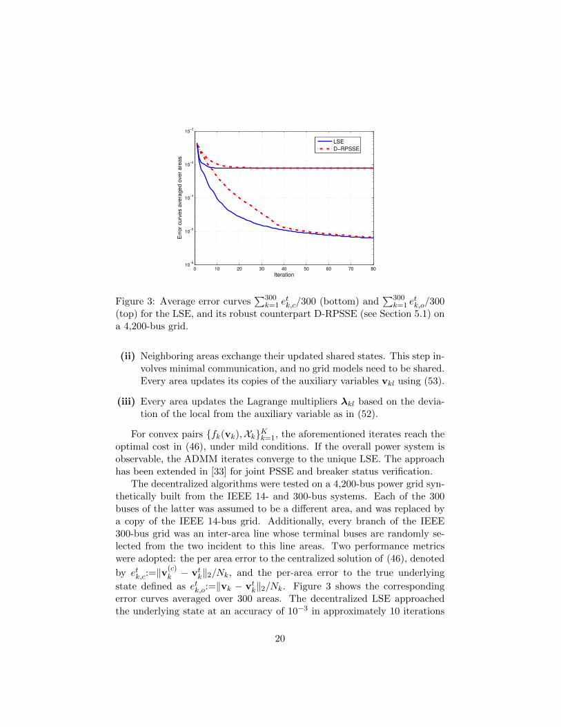
Figure 3: Average error curves∑300

k=1 etk,c/300 (bottom) and

∑300k=1 e

tk,o/300

(top) for the LSE, and its robust counterpart D-RPSSE (see Section 5.1) ona 4,200-bus grid.

(ii) Neighboring areas exchange their updated shared states. This step in-volves minimal communication, and no grid models need to be shared.Every area updates its copies of the auxiliary variables vkl using (53).

(iii) Every area updates the Lagrange multipliers λkl based on the devia-tion of the local from the auxiliary variable as in (52).

For convex pairs {fk(vk),Xk}Kk=1, the aforementioned iterates reach theoptimal cost in (46), under mild conditions. If the overall power system isobservable, the ADMM iterates converge to the unique LSE. The approachhas been extended in [33] for joint PSSE and breaker status verification.

The decentralized algorithms were tested on a 4,200-bus power grid syn-thetically built from the IEEE 14- and 300-bus systems. Each of the 300buses of the latter was assumed to be a different area, and was replaced bya copy of the IEEE 14-bus grid. Additionally, every branch of the IEEE300-bus grid was an inter-area line whose terminal buses are randomly se-lected from the two incident to this line areas. Two performance metricswere adopted: the per area error to the centralized solution of (46), denoted

by etk,c:=‖v(c)k − vtk‖2/Nk, and the per-area error to the true underlying

state defined as etk,o:=‖vk − vtk‖2/Nk. Figure 3 shows the correspondingerror curves averaged over 300 areas. The decentralized LSE approachedthe underlying state at an accuracy of 10−3 in approximately 10 iterations

20

or 6.2 msec on an Intel Duo Core @ 2.2 GHz (4GB RAM) computer usingMATLAB; while the centralized LSE finished in 93.4 msec.

4.2 Distributed SDR-based Estimators

Although the SDR-PSSE approach incurs polynomial complexity when im-plemented as a convex SDP, its worst-case complexity is stillO(M4

√Nb log(1/ε))

for a given solution accuracy ε > 0 [46]. For typical power networks, thenumber of measurements M is on the order of the number of buses Nb, andthus the worst-case complexity becomes O(N4.5

b log(1/ε)). This complexitycould be prohibitive for large-scale power systems, which motivates acceler-ating the SDR-PSSE method using distributed parallel implementations.

Following the area partition in Fig. 2, the m-th measurement per area kcan be written as

zk,m = hk,m(vk) + εk,m = Tr(Hk,mVk) + εk,m, ∀k,m

where Vk denotes a submatrix of V formed by extracting the rows andcolumns corresponding to buses in area k; and likewise for each Hk,m. Dueto the overlap among the subsets of buses, the outer-product Vk of area koverlaps also with Vl for each neighboring area l ∈ Nk, as shown in Fig. 2.

By reducing the measurements at area k to submatrix Vk, one can de-fine the PSSE error cost fk(Vk) :=

∑Mkm=1 [zk,m − Tr(Hk,mVk)]

2 per areak, which only involves the local matrix Vk. Hence, the centralized PSSEproblem in (32) becomes equivalent to

V = arg minV�0

K∑k=1

fk(Vk). (54)

This equivalent formulation effectively expresses the overall PSSE cost as thesuperposition of each local cost fk. Nonetheless, even with such a decom-posable cost, the main challenge to implement (54) in a distributed mannerlies in the PSD constraint that couples the overlapping local matrices {Vk}(cf. Fig. 2). If all submatrices {Vk} were non-overlapping, the cost wouldbe decomposable as in (54), and the PSD of V would boil down to a PSDconstraint per area k, as in

V = arg min{Vk�0}

K∑k=1

fk(Vk). (55)

Similar to PSSE for linearized measurements in (46), the formulation in(55) can be decomposed into sub-problems, thanks to the separable PSD

21

constraints. It is not always equivalent to the centralized (54) though, be-cause the PSD property of all submatrices does not necessarily lead to aPSD overall matrix. Nonetheless, the decomposable problem (55) is stilla valid SDR-PSSE reformulation, since with the additional per-area con-straints rank(Vk) = 1, it is actually equivalent to (30). While it is totallylegitimate to use (55) as the relaxed SDP formulation for (30), the tworelaxed problems are actually equivalent under mild conditions.

The fresh idea here is to explore valid network topologies to facilitatesuch PSD constraint decomposition. To this end, it will be instrumen-tal to leverage results on completing partial Hermitian matrices to obtainPSD ones [24]. Upon obtaining the underlying graph formed by the spec-ified entries in the partial Hermitian matrices, these results rely on theso-termed graph chordal property to establish the equivalence between thepositive semidefiniteness of the overall matrix and that of all submatricescorresponding to the graph’s maximal cliques. Interestingly, this techniquewas recently used for developing distributed SDP-based optimal power flow(OPF) solvers in [28, 12, 42].

Construct first a new graph B′ over B, with all its edges correspondingto the entries in {Vk}. The graph G′ amounts to having all buses withineach subset Nk to form a clique. Furthermore, the following are assumed:

(as4) The graph with all the control areas as nodes, and their edges definedby the neighborhood subset {Nk}Kk=1 forms a tree.

(as5) Each control area has at least one bus that does not overlap with anyneighboring area.

Proposition 3. Under (as4)-(as5), the two relaxed problems (54) and (55)are equivalent.

Proposition 3 can be proved by following the arguments in [84] to showthat the entire PSD matrix V can be “completed” using only the PSDsubmatrices Vk. The key point is that in most power networks even thosenot obeying (as4) and (as5), (55) can achieve the same accuracy as thecentralized one. At the same time, decomposing the PSD constraint in (55)is of paramount importance for developing distributed solvers. One canadopt the consensus reformulation to design the distributed solver for (55) asin (46) of Section 4.1. Accordingly, the ADMM iterations can be employedto solve (55) through iterative information exchanges among neighboringareas, and this is the basis of the distributed SDR-PSSE method.

This distributed SDR-PSSE method was tested on the IEEE 118-bussystem using the three-area partition in [31]. All three areas measure their

22

0 20 40 60 8010

−3

10−2

10−1

100

101

Lo

cal m

atrix

err

or

Iteration index

Area 1Area 2Area 3

0 20 40 60 80

10−1

100

Loca

l est

imat

ion

erro

r

Iteration index

Area 1Area 2Area 3

Figure 4: (Left) Per area state matrix error and (Right) state vector esti-mation error, versus the number of ADMM iterations for the distributedSDR-PSSE solver using the IEEE 118-bus system.

local bus voltage magnitudes, as well as real and reactive power flow levelsat all lines. The overlaps among the three areas form a tree communicationgraph used to construct the area-coupling constraints. To demonstrate con-vergence of the ADMM iterations to the centralized SE solution V of (55),the local matrix Frobenius error norm ‖Vi

(k) − V(k)‖F is plotted versus theiteration index i in the left panel of Fig. 4 for every control area k. Clearly,all local iterates converge to (approximately with a linear rate) their coun-terparts in the centralized solution. As the task of interest is to estimate thevoltages, the local estimation error for the state vector ‖vi(k)−v(k)‖2 is alsodepicted in the right panel of Fig. 4, where v(k) is the estimate of bus volt-

ages at area k obtained from the iterate Vi(k) using the eigen-decomposition

method. Interestingly, the estimation error costs converge within the es-timation accuracy of around 10−2 after about 20 iterations (less than 10iterations for area 1), even though the local matrix has not yet converged.In addition, these error costs decrease much faster in the first couple of itera-tions. This demonstrates that even with only a limited number of iterations,the PSSE accuracy can be greatly boosted in practice, which in turn makesinter-area communication overhead more affordable.

5 Robust Estimators and Cyber Attacks

Bad data, also known as outliers in the statistics parlance, can challengePSSE due to communication delays, instrument mis-calibration, and/or line

23

parameter uncertainty. In today’s cyber-enabled power systems, smart me-ter and synchrophasor data could be also purposefully manipulated to mis-lead system operators. This section reviews conventional and contemporaryapproaches to coping with outliers.

5.1 Bad Data Detection and Identification

Bad data processing in PSSE relies mainly on the linear measurement modelz = Hv + ε, where H ∈ RM×N . Recall that this model is exact for PMUmeasurements [cf. (16)–(17)], but approximate per Gauss-Newton iterationor under the linearized grid model. In addition, the aforementioned modelassumes real-valued states and measurements, slightly abusing the symbolsintroduced in (17). This is to keep the notation uncluttered and cover bothcases of exact and inexact grid models. Albeit the nominal measurementnoise vector is henceforth assumed zero-mean with identity covariance, re-sults extend to colored noise as per (20).

To capture bad data, the measurement model is now augmented as

z = Hv + o + ε (56)

where o ∈ RM is an unknown vector whose m-th entry om is deterministi-cally non-zero only if zm is a bad datum [30, 39, 15]. Therefore, vector o issparse, i.e., many of its entries are zero. Under this outlier-cognizant modelin (56), the unconstrained LSE given as vLSE = (HTH)−1HT z, yields theresidual error

r := z−HvLSE = Pz = P(o + ε) (57)

with P := IM −H(HTH)−1HT being the so-called projection matrix ontothe orthogonal subspace of range(H). The last equality in (57) stems fromthe fact that PH = 0. As a projection matrix, P is idempotent, that is,P = P2; Hermitian PSD with (M − N) eigenvalues equal to one and Nzero eigenvalues; while its diagonal entries satisfy Pm,m ∈ [0, 1] for m =1, . . . , M ; see e.g., [6].

For ε ∼ N (0, IM ), it apparently holds that Pε ∼ N (0,P). The mean-squared residual error is (see also [39] for its Bayesian counterpart)

E[‖r‖22] = E[‖Pε‖22] + ‖Po‖22 = (M −N) + ‖Po‖22. (58)

In the absence of bad data, or if o ∈ range(H), the squared residual errorfollows a χ2 distribution with mean (M − N). The χ2-test compares ‖r‖22against a threshold to detect the presence of bad data [1, 55].

24

Finding both v and o from measurements in (56) may seem impossi-ble, given that the number of unknowns exceeds the number of equations.Leveraging the sparsity of o though, interesting results can be obtained [30].If τ0 bad data are expected, one would ideally wish to solve

{v, o} ∈ arg minv, o

{1

2‖z−Hv − o‖22 : ‖o‖0 ≤ τ0

}. (59)

But the `0-(pseudo) norm ‖o‖0 counting the number of non-zero entries ofo, renders (59) NP-hard in general; see also Definition 2 later in Section 5.2.

For the special case of τ0 = 1, problem (59) can be efficiently handled.Consider the scenario where the only non-zero entry of o is the m-th one,and denote the related v minimizer by v(m). Apparently, the m-th entry of

the o minimizer is om := zm − hTmv(m). This choice nulls the m-th residual

(zm − hTmv(m) − om = 0). With the m-th residual zeroed, the cost in (59)becomes ‖r(m)‖22 := ‖z(m) − H(m)v(m)‖22, where z(m) is obtained from zupon dropping its m-th entry and H(m) by removing the m-th row of H.The problem in (59) is then equivalent to

minimizem

1

2‖r(m)‖22. (60)

Problem (60) can be solved by exhaustively finding all M LSEs excludingone measurement at a time. Fortunately, a classical result from the adaptivefiltering literature relates the error ‖r(m)‖22 to the error attained using alloutlier-free measurements ‖r‖22 := ‖Pz‖22; see e.g., [25, Ch. 9]

‖r‖22 = ‖r(m)‖22 + rmom. (61)

The same result links the a-posteriori error rm to the a-priori error om asrm = Pm,mom. Through these links, solving (60) is equivalent to:

rmax := maximizem

|rm|√Pm,m

. (62)

In words, a single bad datum can be identified by properly normalizing theentries of the original residual vector r = Pz.

Interestingly, the task in (62) coincides with the largest normalized resid-ual (LNR) test that compares rmax to a prescribed threshold to identify asingle bad datum [1, Sec. 5.7]. The threshold is derived after recognizingthat in the absence of bad data, rm/

√Pm,m is standard normal for all m.

The LNR test does not generalize for multiple bad data and problem(59) becomes computationally intractable for larger τ0’s. Heuristically, if

25

a measurement is deemed as outlying, PSSE is repeated after discardingthis bad datum, the LNR test is re-applied, and the process iterates till nocorrupted data are identified. Alternatively, the least-median squares andthe least-trimmed squares estimators have provable breakdown points andsuperior efficiency under Gaussian data; see e.g., [52] and references therein.Nevertheless, their complexity scales unfavorably with the network size.

Leveraging compressed sensing [7], a practical robust estimator can befound if the `0-pseudonorm is surrogated by the convex `1-norm as [30, 31]

minimizev, o

{1

2‖z−Hv − o‖22 : ‖o‖1 ≤ τ1

}(63)

for a preselected constant τ1 > 0, or in its Lagrangian form

{v, o} ∈ arg minv, o

1

2‖z−Hv − o‖22 + λ‖o‖1 (64)

for some tradeoff parameter λ > 0. The estimates of (64) offer joint stateestimation and bad data identification. Even when some measurements aredeemed as corrupted, their effect has been already suppressed. The op-timization task in (64) can be handled by off-the-shelf software or solverscustomized to the compressed sensing setup. When λ → ∞, the minimizero becomes zero, and thus v reduces to the LSE. On the contrary, by let-ting λ → 0+, the solution v coincides with the least-absolute value (LAV)estimator [40, 6, 17, 68]; presented earlier in (37), namely

vLAV := arg minv‖z−Hv‖1. (65)

For finite λ > 0, the v minimizer of (64) is equivalent to Huber’s M-estimator; see [30] and references therein. Based on this connection andfor Gaussian ε, parameter λ can be set to 1.34, which makes the estima-tor 95% asymptotically efficient for outlier-free measurements [50, p. 26].Huber’s estimate can be alternatively expressed as the v-minimizer of [49],minimizev,ω

12‖ω‖

22 + λ‖v−Hv− ω‖1. The bad data identification perfor-

mance of this minimization has been analyzed in [76].Table 1 compares several bad data analysis methods on the IEEE 14-

bus grid of Fig. 2 under the next four scenarios: (S0) no bad data; (S1)bad data on line (4, 7); (S2) bad data on line current (4, 7) and bus volt-age 5; and (S3) bad data on bus voltage 5 and line currents (4, 7) and(10, 11). In all scenarios, bad data are simulated by multiplying the realand imaginary parts of the actual measurement by 1.2. The performancemetric here is the `2-norm between the true state and the PSSE, which is

26

Table 1: Mean-Square Estimation Error in the Presence of Bad Data

Method GA-LSE LSE LNRT Huber’s

(S0) 0.0278 0.0278 0.0286 0.0281

(S1) 0.0313 0.0318 0.0331 0.0322

(S2) 0.0336 0.1431 0.0404 0.0390

(S3) 0.0367 0.1434 0.0407 0.0390

averaged over 1,000 Monte Carlo runs. Four algorithms were tested: (a)an ideal but practically infeasible genie-aided LSE (GA-LSE), which ignoresthe corrupted measurements; (b) the regular LSE; (c) the LNR test-based(LNRT) estimator with the test threshold set to 3.0 [1]; and (d) Huber’sestimator of (64) with λ = 1.34. For (S0)-(S1), the estimators performcomparably. The few corrupted measurements in (S2)-(S3) can deteriorateLSE’s performance, while Huber’s estimator performs slightly better thanLNRT. Computationally, Huber’s estimator was run within 1.3 msec, whilethe LNRT required 1.5 msec. The computing times were also measured forthe IEEE 118-bus grid without corrupted data. Interestingly, the averagetime on the IEEE 118-bus grid without corrupted data are 3.2 msec and81 msec, respectively.

Towards a robust decentralized state estimator, the ADMM-based frame-work of Section 4.1 can be engaged here too. If the measurement model forthe k-th area is zk = Hkvk + ok + εk, the centralized problem boils down to

minimize{vk∈Xk, ok}

K∑k=1

1

2‖zk −Hkvk − ok‖22 + λ‖ok‖1. (66)

To allow for decentralized implementation, the optimization in (66) can bereformulated as

minimizeK∑k=1

1

2‖zk −Hkvk − ok‖22 + λ‖ωk‖1 (67a)

over {vk ∈ Xk, ok, ωk}, {vkl} (67b)

s. to vk[l] = vkl, for all l ∈ Bk, k = 1, . . . ,K. (67c)

ok = ωk, for all k = 1, . . . ,K. (67d)

As in Section 4.1, the constraints in (67c) and the auxiliary variables {vkl}enforce consensus of shared states. On the other hand, the variables {ok}

27

are duplicated as {ωk} in (67d). Then, variables {vk, ok} are put togetherin the x-update of ADMM in (49a), whereas {vkl, ωk} fall into the z-updatein (49b). In this fashion, costs are separable over variable groups, and theminimization involving the `1-norm enjoys a closed-form solution expressedin terms of the soft thresholding operator [31].

5.2 Observability and Cyber Attacks

In the cyber-physical smart grid context, bad data are not simply uninten-tional errors, but can also take the form of malicious data injections [54].Amid these challenges, the intertwined issues of critical measurements andstealth cyber-attacks on PSSE are discussed next.

It has been tacitly assumed so far that the power system is observable. Apower system is observable if distinct states v 6= v′ are mapped to distinctmeasurements h(v) 6= h(v′) under a noiseless setup. Equivalently, if theso-called measurement distance function is defined as [81]

D(h) := minimizev 6=v′

‖h(v)− h(v′)‖0 (68)

the power system is observable if and only if D(h) ≥ 1. Given the networktopology and the mapping h(v), the well-studied topic of observability anal-ysis aims at determining whether the system state is uniquely identifiable,at least locally in a neighborhood of the current estimate [1, Ch. 4]. If not,mapping observable islands, meaning maximally connected sub-grids withobservable internal flows, is important as well.

Observability analysis relies on the decoupled linearized grid model, andis accomplished through topological or numerical tests [8, 56]. Apparently,under the linear or linearized model h(v) = Hv, the state v is uniquelyidentifiable if and only if H is full column-rank. Phase shift ambiguities canbe waived by fixing the angle at a reference bus.

In the presence of bad data and/or cyber attacks, observability analysismay not suffice. Consider the noiseless measurement model z = h(v) + o,where the non-zero entries of vector o correspond to bad data or compro-mised meters; and let us proceed with the following definitions.

Definition 1 (Observable attack [81]). The attack vector o is deemed asobservable if for every state v there is no v′ 6= v, such that h(v)+o = h(v′).

Definition 2 (Identifiable attack [81]). The attack vector o is identifiableif for every v there is no (v′,o′) with v′ 6= v and ‖o′‖0 ≤ ‖o‖0, such thath(v) + o = h(v′) + o′.

28

If the outlier vector o is observable, the operator can tell that the col-lected measurements do not correspond to a system state, and can hencedecide that an attack has been launched. Nevertheless, the attacked meterscan be pinpointed only under the stronger conditions of Definition 2.

The resilience of the measurement mapping h(v) against attacks can becharacterized through D(h) in (68): The maximum number of counterfeitedmeters for an attack to be observable is Ko = D(h)−1 and to be identifiable,

it is Ki = bD(h)−12 c; see [81, 76]. Here, the floor function bxc returns the

greatest integer less than or equal to x.Consider the linear mapping h(v) = Hv. Measurement m is termed

critical if once removed from the measurement set, it renders the powersystem non-identifiable. In other words, although H is full column-rank, itssubmatrix H(m) is not. It trivially follows that D(h) = 1, and the systemoperator can be arbitrarily misled even if only measurement m is attacked.Due to the typically sparse structure of H, critical measurements or multiplesimultaneously corrupted data do exist [1]. It was pointed out in [45] that ifan attack o can be constructed to lie in the range(H), it comprises a ‘stealthattack.’ Although finding D(h) is not trivial in general, a polynomial-timealgorithm leveraging a graph-theoretic approach is devised in [39].

6 Power System State Tracking

The PSSE methods reviewed so far ignore system dynamics and do notexploit historical information. Dynamic PSSE is well motivated thanks to itsimproved robustness, observability, and predictive ability when additionaltemporal information is available [26]. Recently proposed model-free andmodel-based state tracking schemes are outlined next.

6.1 Model-free State Tracking via Online Learning

In complex future power systems, one may not choose to explicitly committo a model for the underlying system dynamics. The framework of onlineconvex optimization (OCO), particularly popular in machine learning, canaccount for unmodeled dynamics and is thus briefly presented next [62].

The OCO model considers a multi-stage game between a player and anadversary. In the PSSE context, the utility or the system operator assumesthe role of the player, while the loads and renewable generations can beviewed as the adversary. At time t, the player first selects an action Vt froma given action set V, and the adversary subsequently reveals a convex loss

29

function ft : V → R. In this round, the player suffers a loss ft(Vt). Theultimate goal for the player is to minimize the regret Rf (T ) over T rounds:

Rf (T ) :=T∑t=1

ft(Vt)−minimizeV∈V

T∑t=1

ft(V). (69)

The regret is basically the accumulated cost incurred by the player relativeto that by a single fixed action V0 := arg minV∈V

∑Tt=1 ft(V). This fixed

action is selected with the advantage of knowing the loss functions {ft}Tt=1

in hindsight. Under appropriate conditions, judiciously designed online op-timization algorithms can achieve sublinear regret; that is, Rf (T )/T → 0 asT → +∞.

Building on the SDR-PSSE formulation of Section 3.4, the ensuing methodconsiders streaming data for real-time PSSE. The data referring to and col-lected over the control period t are {(zmt ; Hmt)}Mt

mt=1 with t = 1, . . . , T .The number and type of measurements can change over time, while the ma-trix corresponding to measurement m may change over time as indicated by{Hmt}Mt

mt=1 due to topology reconfigurations. The online PSSE task can benow formulated as

minimizeV�0

T∑t=1

ft(V) (70)

where ft(V) :=∑Mt

mt=1[zmt −Tr(HmtV)]2. Online PSSE aims at improvingthe static estimates by capitalizing on previous measurements as well astracking slow time-varying variations in generation and demand.

Minimizing the cost in (70) may be computationally cumbersome forreal-time implementation. An efficient alternative based on online gradientdescent amounts to iteratively minimizing a regularized first-order approxi-mation of the instantaneous cost instead [37]

Vt+1 := arg minV�0

Tr(VH∇ft(Vt)) +1

2µt‖V −Vt‖2F (71)

for t = 1, . . ., and suitably selected step sizes µt > 0. Interestingly, theoptimization in (71) admits a closed-form solution given by

Vt+1 = ProjS+ [Vt − µt∇ft(Vt)] (72)

with ProjS+ denoting the projection onto the positive semidefinite cone,which can be performed using eigen-decomposition followed by setting neg-ative eigenvalues to zero. It is worth mentioning that the online PSSE in

30

(72) enjoys sublinear regret [37]. Upon finding Vt, a state estimate vt can beobtained by eigen-decomposition or randomization as in Section 3.4. Withan additional nuclear-norm regularization term promoting low-rank solu-tions in (71), online ADMM alternatives were devised in [36]. Interestingly,online learning tools has recently been advocated for numerous real-timeenergy management tasks in [35], [34], [69].

6.2 Model-based State Tracking

Although the previous model-free solver can recover slow time-varying states,model-based approaches facilitate tracking of fast time-varying system states.A typical state-space model for power system dynamics is [65]

vt+1 = Ftvt + gt + ωt (73a)

zt = h(vt) + εt (73b)

where Ft denotes the state-transition matrix, gt captures the process mis-match, and wt is the additive noise. The nonlinear mapping h(·) comes fromconventional SCADA measurements. Values {(Ft,gt)} can be obtained inreal-time using for example Holt’s system identification method [11]. Twocommon dynamic tracking approaches to cope with the nonlinearity in themeasurement model of (73b) include the (extended or unscented) Kalmanfilters and moving horizon estimators [65, 14, 26, 73, 72], and they are out-lined in order next.

The extended Kalman filter (EKF) handles the nonlinearity by lineariz-ing h(v) around the state predictor. To start, let vt+1|t stand for the pre-dicted estimate at time t + 1 given measurements {zτ}tτ=1 up to time t.Let also vt+1|t+1 be the filtered estimate given measurements {zτ}t+1

τ=1. Ifthe noise terms ωt and εt in (73) are assumed zero-mean Gaussian withknown covariance matrices Qt � 0 and Rt � 0, respectively, the EKF canbe implemented with the following recursions

vt+1|t+1 = vt+1|t + Kt+1

[zt+1 − h(vt+1|t)

](74)

where the state predictor vt+1|t and the Kalman gain Kt+1 are given by

vt+1|t = Ftvt|t + gt (75a)

Kt+1 = Pt+1|tJHt+1

(Jt+1Pt+1|tJ

Ht+1 + Rt+1

)−1(75b)

Pt+1|t+1 = Pt+1|t −Kt+1Jt+1Pt+1|t (75c)

Pt+1|t = FtPt|tFHt + Qt (75d)

31

with Jt+1 being the measurement Jacobian matrix of h evaluated at vt+1|t,and Pt+1|t+1 � 0 (Pt+1|t � 0) denoting the corrected (predicted) stateestimation error covariance matrix at time t+ 1. To improve on the approx-imation accuracy of the EKF, extended Kalman filters (UKF) have beenreported in [65]; see also [79] for their robust versions. Particle filteringmay also be useful if its computational complexity can be supported duringreal-time power systems operations.

Because the EKF and UKF are known to diverge for highly nonlineardynamics, moving horizon estimation (MHE) has been suggested as an ac-curate yet tractable alternative with proven robustness to bounded modelerrors [59]. Different from Kalman filtering, the initial state v0, and noisesωt and εt in MHE are viewed as deterministic unknowns taking values fromgiven bounded sets S, W, and E , respectively. The sets W and E modeldisturbances with truncated densities [59].

The idea behind MHE is to perform PSSE by exploiting useful informa-tion present in a sliding window of the most recent observations. Considerhere a sliding window of length L + 1. Let vt−L|t denote the smoothedestimate at time t − L given L past measurements, as well as the cur-rent one, namely {zτ}tτ=t−L. MHE aims at obtaining the most recent Lstate estimates {vt−L+s|t}Ls=0 based on {zτ}tt−L and the available estimatevt−L := vt−L|t−1 from time t− 1 and for t ≥ L. A key simplification is thatonce vt−L|t becomes available, the other L recent estimates at time t can berecursively obtained through ‘noise-free’ propagation based on the dynamicmodel (73a); that is,

vt−L+s|t = Ft−L+s−1vt−L+s−1|t (76)

for s = 1, . . . , L. By relating all recent estimates to vt−L|t via successivemultiplications of transition matrices, the update in (76) simplifies to

vt−L+s|t = Tt−L+svt−L|t (77)

where Tt−L+s := Ft−L+s−1Tt−L+s−1 for s = 1, . . . , L, with Tt−L = I. TheMHE-based state estimate vt−L|t is then given by

vt−L|t := arg minv

L∑s=0

∥∥zt−L+s − h(Tt−L+sv)∥∥22

+ λ‖v − vt−L‖22 (78)

where λ > 0 can be tuned relying on our confidence in the state predictorvt−L, and the measurements {zτ}tt−L. Given the quadratic dependence of

32

the SCADA measurements {h(vt)} and the state v, the optimization prob-lem in (78) is non-convex.

Finding the MHE-based state estimates in real time entails online so-lutions of dynamic optimization problems. The MHE formulation can beconvexified by exploiting the semidefinite relaxation: vector v is lifted to thematrix V := vvH � 0, and the m-th entry of h(vt−L+s) for s = 0, . . . , L, isexpressed as

hm(Tt−L+sv) = vHTHt−L+sHmTt−L+sv = Tr(THt−L+sHmTt−L+sV).

Upon dropping the nonconvex rank constraint rank(V) = 1, the SDP-basedMHE yields

Vt−L|t := arg minV�0

L∑s=0

∥∥zt−L+s−Tr(THt−L+sHmTt−L+sV

)∥∥22+λ‖v−vt−L‖22

which can be solved in polynomial time using off-the-shelf toolboxes. Rank-one state estimates can be obtained again through eigen-decomposition orrandomization. The complexity of solving the last problem is rather highin its present form on the order of N4.5

b [46]. Therefore, developing fastersolvers for the SDP-based MHE by exploiting the rich sparsity structure in{Hm} matrices is worth investigating. Decentralized and localized MHEimplementations are also timely and pertinent. Devising FPP-based solversfor the MHE in (78) constitutes another research direction.

7 Discussion

This chapter has reviewed some of the recent advances in PSSE. After de-veloping the CRLB, an SDP-based solver, and its regularized counterpartwere discussed. To overcome the high complexity involved, a scheme namedfeasible point pursuit relying on successive convex approximations was alsoadvocated. A decentralized PSSE paradigm put forth provides the meansfor coping with the computationally-intensive SDP formulations, it is tai-lored for the interconnected nature of modern grids, while it can also affordprocessing PMU data in a timely fashion. A better understanding of cyberattacks and disciplined ways for decentralized bad data processing were alsoprovided. Finally, this chapter gave a fresh perspective to state trackingunder model-free and model-based scenarios.

Nonetheless, there are still many technically challenging and practicallypertinent grid monitoring issues to be addressed. Solving power grid data

33

processing tasks on the cloud has been a major trend to alleviate data stor-age, communication, and interoperability costs for system operators andutilities. Moreover, with the current focus on low- and medium-voltage dis-tribution grids, solvers for unbalanced and multi-phase operating conditions[2] are desirable. Smart meters and synchrophasor data from distributiongrids (also known as micro-PMUs [67]) call for new data processing solu-tions. Advances in machine learning and statistical signal processing, suchas sparse and low-rank models, missing and incomplete data, tensor decom-positions, deep learning, nonconvex and stochastic optimization tools, and(multi)kernel-based learning to name a few, are currently providing novelpaths to grid monitoring tasks while realizing the vision of smarter energysystems.

Acknowledgements

G. Wang and G. B. Giannakis were supported in part by NSF grants 1423316,1442686, 1508993, and 1509040; and by the Laboratory Directed Researchand Development Program at the NREL. H. Zhu was supported in part byNSF grants 1610732 and 1653706.

Appendix

Proof of Prop. 1. Consider the AGWN model (15) with ε ∼ N (0,dg({σ2m})).The data likelihood function is

p(z; v) =M∏m=1

1√2πσ2m

exp

[−(zm − vHHmv)2

2σ2m

](79)

and the negative log-likelihood function denoted by f(v) = − ln p(z; x) is

f(v) =

M∑m=1

[1

2σ2m

(zm − vHHmv

)2+

1

2ln(2πσ2m

)]. (80)

The Fisher information matrix (FIM) is defined as the Hessian of thereal-valued function f(v) with respect to the complex vector v ∈ CNb . De-riving the CRLB amounts to finding the Hessian of a real-valued functionwith respect to a complex-valued vector. Wirtinger’s calculus confirms thatf(v) can be equivalently rewritten as f(v,v∗); see e.g., [41]. Upon intro-ducing the conjugate coordinates [vT (v∗)T ]T ∈ C2Nb , the Wirtinger deriva-tives, namely the first-order partial differential operators of functions over

34

complex domains, are given by [41]

∂f

∂v:=

∂f(v,v∗)

∂vT

∣∣∣∣constant v∗

=

[∂f

∂V1· · · ∂f

∂VN

]∣∣∣∣constant v∗

∂f

∂v∗:=

∂f(v,v∗)

∂(v∗)T

∣∣∣∣constant v

=

[∂f

∂V∗1· · · ∂f

∂V∗N

]∣∣∣∣constant v

.

These definitions follow the convention in multivariate calculus that deriva-tives are denoted by row vectors, and gradients by column vectors. Definefor notational brevity φm(v,v∗) := zm − (v∗)THmv for m = 1, . . . ,M .Accordingly, the Wirtinger derivatives of f(v,v∗) in (80) are obtained as

∂f

∂v=

M∑m=1

1

σ2mφm

∂φm∂vT

and∂f

∂v∗=

L∑m=1

1

σ2mφm

∂φm∂(v∗)T

(82)

and the Wirtinger derivatives of φm(v,v∗) can be found likewise

∂φm∂vT

= −(Hmv)H and∂φm∂(v∗)T

= −(H∗mv∗)H. (83)

In the conjugate coordinate system, the complex Hessian of f(v,v∗) withrespect to the conjugate coordinates [vT (v∗)T ]T is defined as

H(v,v∗) := ∇2f(v,v∗) =

[Hvv Hv∗v

Hvv∗ Hv∗v∗

](84)

whose blocks are given as

Hvv :=∂

∂vT

(∂f

∂v

)H, Hv∗v :=

∂

∂(v∗)T

(∂f

∂v

)HHvv∗ :=

∂

∂vT

(∂f

∂v∗

)H, Hv∗v∗ :=

∂

∂(v∗)T

(∂f

∂v∗

)H.

Substituting (82) and (83) into the last equations and after algebraic ma-nipulations yields

Hvv =

M∑m=1

σ−2m

(Hmv(Hmv)H − φmHm

)(85a)

Hv∗v =

M∑m=1

σ−2m Hmv(H∗mv∗)H (85b)

35

Hvv∗ =

M∑m=1

σ−2m H∗mv∗(Hmv)H (85c)

Hv∗v∗ =M∑m=1

σ−2m

(H∗mv∗(H∗mv∗)H − φmH∗m

). (85d)

Evaluating the Hessian blocks of (85) at the true value of v, and takingthe expectation with respect to ε, yields E[φm] = 0. Hence, the φm-relatedterms in (85) disappear, and the FIM F(v,v∗) := E[H(v,v∗)] simplifies tothe expression in (23); see also [66].

To show that the FIM is rank-deficient, define gm := [(Hmv)H (H∗mv∗)H]H,so that the FIM becomes F =

∑Mm=1 σ

−2m gmgHm. Observe now that the non-

zero vector d(v) := [vT − (v∗)T ]T is orthogonal to gm for m = 1, . . . ,M ;that is,

gHmd = vHHmv − (vHHmv)∗ = 0.

Based on the latter, it is not hard to verify that Fd = 0, which proves thatthe null space of F is non-empty.

References

[1] A. Abur and A. Gomez-Exposito, Power System State Estimation: The-ory and Implementation. New York, NY: Marcel Dekker, 2004.

[2] M. Bazrafshan and N. Gatsis, “Comprehensive modeling of three-phasedistribution systems via the bus admittance matrix,” arXiv:1705.06782,2017.

[3] D. P. Bertsekas, Nonlinear Programming, 2nd ed. Belmont, MA:Athena Scientific, 1999.

[4] S. Boyd, N. Parikh, E. Chu, B. Peleato, and J. Eckstein, “Dis-tributed optimization and statistical learning via the alternating di-rection method of multipliers,” Found. Trends Mach. Learn., vol. 3,pp. 1–122, 2010.

[5] S. Boyd and L. Vandenberghe, Convex Optimization. New York, NY:Cambridge University Press, 2004.

[6] M. K. Celik and A. Abur, “A robust WLAV state estimator using trans-formations,” IEEE Trans. Power Syst., vol. 7, no. 1, pp. 106–113, Feb.1992.

36

[7] S. S. Chen, D. L. Donoho, Michael, and A. Saunders, “Atomic decom-position by basis pursuit,” SIAM J. Sci. Comput., vol. 20, pp. 33–61,Jul. 1998.

[8] K. A. Clements, G. R. Krumpholz, and P. W. Davis, “Power sys-tem state estimation with measurement deficiency: An observabil-ity/measurement placement algorithm,” IEEE Trans. Power App.Syst., vol. 102, no. 7, pp. 2012–2020, Jul. 1983.

[9] A. J. Conejo, S. de la Torre, and M. Canas, “An optimization approachto multiarea state estimation,” IEEE Trans. Power Syst., vol. 22, no. 1,pp. 213–221, Feb. 2007.

[10] T. V. Cutsem and M. Ribbens-Pavella, “Critical survey of hierarchicalmethods for state estimation of electric power systems,” IEEE Trans.Power App. Syst., vol. 102, no. 10, pp. 3415–3424, Oct. 1983.

[11] A. L. Da Silva, M. Do Coutto Filho, and J. De Queiroz, “State forecast-ing in electric power systems,” IEE Proc. Generat. Transm. Distrib.,vol. 130, no. 5, pp. 237–244, Sep. 1983.

[12] E. Dall’Anese, H. Zhu, and G. B. Giannakis, “Distributed optimalpower flow for smart microgrids,” IEEE Trans. Smart Grid, vol. 4,no. 3, pp. 1464–1475, Sep. 2013.

[13] J. De La Ree, V. A. Centeno, J. Thorp, and A. Phadke, “Synchro-nized phasor measurement applications in power systems,” IEEE Trans.Smart Grid, vol. 1, no. 1, pp. 20–27, Jun. 2010.

[14] A. S. Debs and R. E. Larson, “A dynamic estimator for tracking thestate of a power system,” IEEE Trans. Power App. Syst., no. 7, pp.1670–1678, Sep. 1970.

[15] D. Duan, L. Yang, and L. L. Scharf, “Phasor state estimation fromPMU measurements with bad data,” in Proc. IEEE Workshop onComp. Adv. in Multi-Sensor Adaptive Proc., San Juan, Puerto Rico,Dec. 2011.

[16] R. Ebrahimian and R. Baldick, “State estimation distributed process-ing,” IEEE Trans. Power Syst., vol. 15, no. 4, pp. 1240–1246, Nov.2000.

37

[17] A. A. El-Keib, J. Nieplocha, H. Singh, and D. Maratukulam, “A de-composed state estimation technique suitable for parallel processor im-plementation,” IEEE Trans. Power Syst., vol. 7, no. 3, pp. 1088–1097,Aug. 1992.

[18] D. M. Falcao, F. F. Wu, and L. Murphy, “Parallel and distributed stateestimation,” IEEE Trans. Power Syst., vol. 10, no. 2, pp. 724–730, May1995.

[19] G. B. Giannakis, V. Kekatos, N. Gatsis, S.-J. Kim, H. Zhu, and B. Wol-lenberg, “Monitoring and optimization for power grids: A signal pro-cessing perspective,” IEEE Signal Process. Mag., vol. 30, no. 5, pp.107–128, Sept. 2013.

[20] G. B. Giannakis, Q. Ling, G. Mateos, I. D. Schizas, and H. Zhu, “Decen-tralized learning for wireless communications and networking,” Split-ting Methods in Communication, Imaging, Science, and Engineering,pp. 461–497, Springer, 2016.

[21] M. X. Goemans and D. P. Williamson, “Improved approximation algo-rithms for maximum cut and satisfiability problems using semidefiniteprogramming,” J. ACM, vol. 42, no. 6, pp. 1115–1145, Nov. 1995.

[22] A. Gomez-Exposito, A. Abur, A. de la Villa Jaen, and C. Gomez-Quiles,“A multilevel state estimation paradigm for smart grids,” Proc. IEEE,vol. 99, no. 6, pp. 952–976, Jun. 2011.

[23] A. Gomez-Exposito, A. de la Villa Jaen, C. Gomez-Quiles,P. Rousseaux, and T. V. Cutsem, “A taxonomy of multi-area stateestimation methods,” Electr. Pow. Syst. Res., vol. 81, pp. 1060–1069,Apr. 2011.

[24] R. Grone, C. R. Johnson, E. M. Sa, and H. Wolkowicz, “Positive definitecompletions of partial hermitian matrices,” Linear Algebra & its Appl.,vol. 58, pp. 109–124, Apr. 1984.

[25] S. Haykin, Adaptive Filter Theory. New York, NY: Prentice Hall, 2002.

[26] S.-J. Huang and K.-R. Shih, “Dynamic-state-estimation scheme includ-ing nonlinear measurement function considerations,” IEE Proc. Gen-erat. Transm. Distrib., vol. 149, no. 6, pp. 673–678, Nov. 2002.

38

[27] S. Iwamoto, M. Kusano, and V. H. Quintana, “Hierarchical state es-timation using a fast rectangular-coordinate method,” IEEE Trans.Power Syst., vol. 4, no. 3, pp. 870–880, Aug. 1989.

[28] R. A. Jabr, “Exploiting sparsity in SDP relaxations of the OPF prob-lem,” IEEE Trans. Power Syst., vol. 27, no. 2, pp. 1138–1139, May2012.

[29] S. M. Kay, Fundamentals of Statistical Signal Processing, Vol. I: Esti-mation Theory. Prentice Hall, 1993.

[30] V. Kekatos and G. B. Giannakis, “From sparse signals to sparse resid-uals for robust sensing,” IEEE Trans. Signal Process., vol. 59, no. 7,pp. 3355–3368, Jul. 2011.

[31] ——, “Distributed robust power system state estimation,” IEEE Trans.Power Syst., vol. 28, no. 2, pp. 1617–1626, May 2013.

[32] V. Kekatos, G. B. Giannakis, and B. F. Wollenberg, “Optimal place-ment of phasor measurement units via convex relaxation,” IEEE Trans.Power Syst., vol. 27, no. 3, pp. 1521–1530, Aug. 2012.

[33] V. Kekatos, E. Vlachos, D. Ampeliotis, G. B. Giannakis, andK. Berberidis, “A decentralized approach to generalized power sys-tem state estimation,” in Proc. IEEE Wkshp. on Comp. Adv. in Multi-Sensor Adaptive Proc., Saint Martin, Dec. 2013.

[34] V. Kekatos, G. Wang, A. J. Conejo, and G. B. Giannakis, “Stochas-tic reactive power management in microgrids with renewables,” IEEETrans. Power Syst., vol. 30, no. 6, pp. 3386–3395, Nov. 2015.

[35] S. J. Kim, G. B. Giannakis, and K. Y. Lee, “Online optimal power flowwith renewables,” in Asilomar Conf. on Signals, Syst. and Comput.,Pacific Grove, CA, Nov 2014, pp. 355–360.

[36] S.-J. Kim, “Online power system state estimation using alternatingdirection method of multipliers,” in Proc. IEEE PES Summer Meeting,Denver, CO, 2015.

[37] S.-J. Kim, G. Wang, and G. B. Giannakis, “Online semidefinite pro-gramming for power system state estimation,” in Proc. IEEE Intl. Conf.on Acoustics, Speech, and Signal Process., Florence, Italy, May 2014,pp. 6024–6027.

39

[38] G. N. Korres, “A distributed multiarea state estimation,” IEEE Trans.Power Syst., vol. 26, no. 1, pp. 73–84, Feb. 2011.

[39] O. Kosut, L. Jia, J. Thomas, and L. Tong, “Malicious data attacks onthe smart grid,” IEEE Trans. Smart Grid, vol. 2, no. 4, pp. 645–658,Dec. 2011.

[40] W. W. Kotiuga and M. Vidyasagar, “Bad data rejection properties ofweighted least-absolute-value techniques applied to static state estima-tion,” IEEE Trans. Power App. Syst., no. 4, pp. 844–853, Apr. 1982.

[41] K. Kreutz-Delgado, “The complex gradient operator and the CR-calculus,” arXiv:0906.4835, 2009.

[42] A. Y. Lam, B. Zhang, and T. David, “Distributed algorithms for opti-mal power flow problem,” in Proc. IEEE Conf. on Decision and Control,Maui, HI, Dec. 2012, pp. 430–437.

[43] S.-Y. Lin and C.-H. Lin, “An implementable distributed state estima-tor and distributed bad data processing schemes for electric power sys-tems,” IEEE Trans. Power Syst., vol. 9, no. 3, pp. 1277–1284, Aug.1994.

[44] T. Lipp and S. Boyd, “Variations and extension of the convex–concaveprocedure,” Optim. Eng., vol. 17, no. 2, pp. 263–287, Jun. 2016.

[45] Y. Liu, P. Ning, and M. K. Reiter, “False data injection attacks againststate estimation in electric power grids,” ACM Trans. Info. and SystemSecurity, vol. 14, no. 1, pp. 13:1–13:33, May 2011.

[46] Z.-Q. Luo, W.-K. Ma, A. M.-C. So, Y. Ye, and S. Zhang, “Semidefiniterelaxation of quadratic optimization problems,” IEEE Signal Process.Mag., vol. 27, no. 3, pp. 20–34, May 2010.

[47] R. Madani, A. Ashraphijuo, J. Lavaei, and R. Baldick, “Power systemstate estimation with a limited number of measurements,” in Proc.IEEE Conf. on Decision and Control, Las Vegas, NV, Dec. 2016.

[48] R. Madani, J. Lavaei, and R. Baldick, “Convexification of power flowproblem over arbitrary networks,” in Proc. IEEE Conf. on Decisionand Control, Osaka, Japan, Dec. 2015.

[49] O. L. Mangasarian and D. R. Musicant, “Robust linear and supportvector regression,” IEEE Trans. Pattern Anal. Mach. Intell., vol. 22,no. 9, pp. 950–955, Sep. 2000.

40

[50] R. A. Maronna, R. D. Martin, and V. J. Yohai, Robust Statistics: The-ory and Methods. Wiley, 2006.

[51] O. Mehanna, K. Huang, B. Gopalakrishnan, A. Konar, andN. Sidiropoulos, “Feasible point pursuit and successive approximationof non-convex QCQPs,” vol. 22, no. 7, pp. 804–808, Nov. 2015.

[52] L. Mili, M. G. Cheniae, and P. J. Rousseeuw, “Robust state estimationof electric power systems,” IEEE Trans. Circuits Syst. I, vol. 41, no. 5,pp. 349–358, May 1994.

[53] A. Minot, Y. M. Lu, and N. Li, “A distributed Gauss-Newton methodfor power system state estimation,” IEEE Trans. Power Syst., vol. 31,no. 5, pp. 3804–3815, Sep. 2016.

[54] B. Y. Mo, T. H.-J. Kim, K. Brancik, D. Dickinson, H. Lee, A. Perrig,and B. Sinopoli, “Cyber-physical security of a smart grid infrastruc-ture,” Proc. IEEE, vol. 100, no. 1, pp. 195–209, Jan. 2012.

[55] A. Monticelli, “Electric power system state estimation,” Proc. IEEE,vol. 88, no. 2, pp. 262–282, Feb. 2000.

[56] A. Monticelli and F. F. Wu, “Network observability: Theory,” IEEETrans. Power App. Syst., vol. 104, no. 5, pp. 1042–1048, May 1985.

[57] P. M. Pardalos and S. A. Vavasis, “Quadratic programming with onenegative eigenvalue is NP-hard,” J. Global Optim., vol. 1, no. 1, pp.15–22, Mar. 1991.

[58] A. G. Phadke and J. S. Thorp, Synchronized Phasor Measurements andTheir Applications. New York, NY: Springer, 2008.

[59] C. V. Rao, J. B. Rawlings, and D. Q. Mayne, “Constrained state esti-mation for nonlinear discrete-time systems: Stability and moving hori-zon approximations,” IEEE Trans. Autom. Contr., vol. 48, no. 2, pp.246–258, Feb. 2003.

[60] I. D. Schizas, A. Ribeiro, and G. B. Giannakis, “Consensus in ad hocWSNs with noisy links: Part I: Distributed estimation of deterministicsignals,” IEEE Trans. Signal Process., vol. 56, no. 1, pp. 350–364, Jan.2008.

[61] F. C. Schweppe, J. Wildes, and D. Rom, “Power system static stateestimation: Parts I, II, and III,” IEEE Trans. Power App. Syst., vol. 89,pp. 120–135, Jan. 1970.

41

[62] S. Shalev-Shwartz, “Online learning and online convex optimization,”Found. and Trends Mach. Learning, vol. 4, no. 2, pp. 107–194, Mar.2011.

[63] P. Stoica and T. L. Marzetta, “Parameter estimation problems withsingular information matrices,” IEEE Trans. Signal Process., vol. 49,no. 1, pp. 87–90, Jan. 2001.

[64] Power systems test case archive. Univ. of Washington. [Online].Available: http://www.ee.washington.edu/research/pstca/

[65] G. Valverde and V. Terzija, “Unscented Kalman filter for power systemdynamic state estimation,” IEE Proc. Generat. Transm. Distrib., vol. 5,no. 1, pp. 29–37, Jan. 2011.

[66] A. Van den Bos, “A Cramer-Rao lower bound for complex parameters,”IEEE Trans. Signal Process., vol. 40, no. 10, Oct. 1994.

[67] A. Von Meier, D. Culler, A. McEachern, and R. Arghandeh, “Micro-synchrophasors for distribution systems,” in Proc. IEEE Conf. on In-novative Smart Grid Technologies, 2014, pp. 1–5.

[68] G. Wang, G. B. Giannakis, and J. Chen, “Robust and scalable powersystem state estimation via composite optimization,” preprint, 2017.

[69] G. Wang, V. Kekatos, A. J. Conejo, and G. B. Giannakis, “Ergodic en-ergy management leveraging resource variability in distribution grids,”IEEE Trans. Power Syst., vol. 31, no. 6, pp. 4765–4775, Nov. 2016.

[70] G. Wang, A. S. Zamzam, G. B. Giannakis, and N. D. Sidiropoulos,“Power system state estimation via feasible point pursuit,” in Proc.IEEE Global Conf. on Signal and Inf. Process., Washington, D.C., Nov.2016.

[71] ——, “Power system state estimation via feasible point pursuit: Algo-rithms and Crmer-Rao bound,” arXiv:1203.0853, 2017.

[72] G. Wang, S.-J. Kim, and G. B. Giannakis, “Moving-horizon dynamicpower system state estimation using semidefinite relaxation,” in Proc.IEEE PES General Meeting, Washington, DC, Jul. 2014, pp. 1–5.

[73] S. Wang, W. Gao, and A. S. Meliopoulos, “An alternative method forpower system dynamic state estimation based on unscented transform,”IEEE Trans. Power Syst., vol. 27, no. 2, pp. 942–950, May 2012.

42

[74] A. J. Wood and B. F. Wollenberg, Power Generation, Operation, andControl, 2nd ed. New York, NY: Wiley & Sons, 1996.

[75] L. Xie, D.-H. Choi, and S. Kar, “Cooperative distributed state esti-mation: Local observability relaxed,” in Proc. IEEE Power & EnergySociety General Meeting, Detroit, MI, Jul. 2011.

[76] W. Xu, M. Wang, J. F. Cai, and A. Tang, “Sparse error correctionfrom nonlinear measurements with applications in bad data detectionfor power networks,” IEEE Trans. Signal Process., vol. 61, no. 24, pp.6175–6187, Dec. 2013.

[77] A. S. Zamzam, N. D. Sidiropoulos, and E. Dall’Anese, “Beyond relax-ation and Newton-Raphson: Solving AC OPF for multi-phase systemswith renewables,” IEEE Trans. Smart Grid, 2017.

[78] Y. Zhang, R. Madani, and J. Lavaei, “Conic relaxations for power sys-tem state estimation with line measurements,” IEEE Trans. ControlNetw. Syst., 2017 (to appear).

[79] J. Zhao, M. Netto, and L. Mili, “A robust iterated extended Kalmanfilter for power system dynamic state estimation,” IEEE Trans. PowerSyst., 2016 (to appear).

[80] L. Zhao and A. Abur, “Multiarea state estimation using synchronizedphasor measurements,” IEEE Trans. Power Syst., vol. 20, no. 2, pp.611–617, May 2005.

[81] H. Zhu and G. B. Giannakis, “Robust power system state estimationfor the nonlinear AC flow model,” in Proc. North American PowerSymposium, Urbana-Champaign, IL, Sep. 2012.

[82] H. Zhu, G. B. Giannakis, and A. Cano, “Distributed in-network decod-ing,” IEEE Trans. Signal Process., vol. 57, no. 10, pp. 3970–3983, Oct.2009.

[83] H. Zhu and G. B. Giannakis, “Estimating the state of AC power sys-tems using semidefinite programming,” in Proc. North American PowerSymposium, Boston, MA, Aug. 2011.

[84] ——, “Power system nonlinear state estimation using distributedsemidefinite programming,” IEEE J. Sel. Topics Signal Process., vol. 8,no. 6, pp. 1039–1050, Dec. 2014.

43