1

PSY 311- MEASUREMENT AND EVALUATION

MOI UNIVERSITY.

THIRD YEAR-SECOND SEMESTER.

COURSE OUTLINE.

Lecturer(s): Mr. kiptala/Mr. Okero

INTRODUCTION

This part of the course will be covered within half a semester (six weeks). The method of teaching will consist of three lectures per week.

The course is concerned with behavioral statistics, measurement and classroom assessment in which the following main topics will be covered;

1. Measurement and its significance in the behavioral studies.

2. Statistics –descriptive and inferential statistics, graphical representation of statistical data.

3. Measures of association or relationship. 4. Measurement of dispersion or spread.

COURSE OBJECTIVES

1. Differentiate among the following important terms; measurement, evaluation and tests/assessment.

2. Identify the various characteristics of measurement variables and their significance.

3. Discuss the various types of scales and their significance to behavioral studies. 4. Discuss the various methods of data presentation. 5. Discuss the measures of central tendency and their significance to behavioral

statistics. 6. Discuss the various measures of variability and standard scores.

EVALUATION

The evaluation of the course will consist of;

• A project and or a continuous assessment test (C.A.T)- 30% • Final university examination -70%

2

COURSE CONTENT

Topic 1 Introduction

• Topics, Key words and terminologies. • Significance of measurement and evaluation. • Characteristics of measurement. • Scales of measurement.

Topic 2 Methods of data presentation

• Data matrix method. • Construction of a frequency distribution table. • Graphical representation of frequency distribution-histogram, frequency

polygon, • Qualities of shape. • Cumulative frequency distribution.

Topic 3 Measures of central tendency.

• Mean • Mode • Median • Relationship between measures of central tendency.

Topic 4 Measures of variability

• Range • Semi-interquartile range • Mean deviation • Standard deviation

Topic 5 Standard scores

• Z-scores • T-scores

Topic 6 The normal curve

• Significance to behavioral statistics. REFERENCE

1. Broadfoot, p. (ed) (1980); Selection, Certification and Control(ed); the Falmer Press, London.

2. Eisner, e. w. (1985); The Art of Educational Evaluation, A Personal View, The Falmer press, London.

3. Hopkins, K.D. and Stanly, j. C. (1981); Educational and Psychological Measurement and Evaluation, Prentice-Hall Inc. New Jersey

4. Lehman I.J. and Mehrens, W.A. (1984); Measurement and evaluation in Education and Psychology (3rd ed), CBS College Publications Co., New York.

3

5. Mathew, j. C. (1985); Examinations Commentary, George Allan and Unwin, London.

6. Kombo, D. K. & Tromp D. L.(2006); Proposal and Thesis Writing, Paulines Publications Africa, Nairobi.

7. Coon D. (2005); psychology a journey, Vicki Knight, Belmont, USA. 8. Thorndike R. M.(2005); Measurement and Evaluation in Psychology and Education

(6th ed), Pearson Education, Inc, New Jersey.

TOPIC ONE

INTRODUCTION

• We frequently make decisions at all levels; be it at home or school and generally every day in life. The more we know about the factors involved in the decisions, the better the decisions are likely to be.

• These decisions should be based on a test or measurement-empirical evidence. • The information at hand must be appropriate for the very decision to be made

and the decision maker must know how best to use the information and what inferences it does and does not support i.e., we will examine:-

1. Key concepts 2. Key practices 3. Methods

That have been developed in education and psychology to aid in decision making i.e., what is it that helps us in decision making. Some decision like

1. This child is fit for this class 2. Personality type 3. Achievement 4. Instructional techniques 5. Behavioural

• Psychological researchers generally follow a scientific approach • This involves the logic of testing hypotheses produced from falsifiable theories. • When enrolling for a course in psychology, the prospective student is very often

taken aback by the discovery that the syllabus includes a fair-sized dollop of statistics and that practical research; experiments and report writing are all involved.

• It is strange that of all sciences-natural and social-the one which directly concerns ourselves as individuals in society is the least likely to be found in schools, where teachers are preparing young people for social life, amongst other things! It is also strange that a student can study all the hard sciences-physics, chemistry and biology-yet never be asked to consider what a science is until they study psychology or sociology.

4

THE HISTORICAL PERSPECTIVE • Formal evaluation of education achievement and the use of this information to

make decisions is an old practice. The Chinese for instance had developed a system of testing and evaluation much earlier than 1800 which resembled the best of modern practice. It served as a model for civil service exams in Western Europe and America during the 1800.

• Although the widespread use of psychological testing is largely a phenomenon of the 20th century, it has been noted that rudimentary forms of testing date back to at least 2200 B.C., when the Chinese emperor had his officials examined every third year to determine their fitness for office (Gregory, 1992).

• Such testing was modified and refined over the centuries until written exams were introduced in the Han dynasty.

• The Chinese examination system took its final form about 1370 when proficiency in the Confusian Classics was emphasized.

• The examinations were grueling and rigorous (e.g., spend a day and a night in a small isolated booth composing essays on assigned topics and writing a poem).

• Those who passed the hierarchical examinations became mandarins or eligible for public office (Gregory, 1992). However, the similarities between the ancient Chinese traditions and current testing practices are superficial.

• Formal measurement procedure began to appear in western educational practice during the 19th century.

• Herman Ebbinghaus came up with a completion test 1896; prior to that it was only essay and oral exams that were used to evaluate or measure students achievement-as a way of measuring mental fatigue in students.

• In 1897 Joseph Rice used the 1st uniform written exams to test spelling achivemenmt of students in public schools in Boston.

• He demonstrated that the amount of time devoted to spelling drills was not related to achievement in spelling.

• He concluded that the time could be reduced and used to teach science. • Rice’s study was used to make a curricula decision. • The second half of the century (19th) saw increased interest in measuring human

characteristics . • Guster Fechner undertook to measure sensory processes. He laid the logical

foundation for psychological and educational measurement. • Sir Francis Galton and Carl Pearson came up with the correlation coefficient in

the service of research on the distribution and causes of human differences. (a & b go along)

• There came the Dubois period of the 1970’s, also known as the laboratory period (when things were being discovered) in the history of psychological measurement; also known as the era of brass instrument psychology because mechanical devices were used to collect measurements of physical and sensory characteristics.

5

Timeline of Early Milestones in the History of Testing

• 2200 B.C.: Chinese emperor examined his officials every third year to determine their fitness for office.

• 1862 A.D.: Wilhelm Wundt uses a calibrated pendulum to measure the “speed of thought”.

• 1869: Scientific study of individual differences begins with the publication of Francis Galton’s Classification of Men According to Their Natural Gifts.

• 1879: Wundt establishes the first psychological laboratory in Leipzig, Germany. • 1884: Galton administers the first test battery to thousands of citizens at the

International Health Exhibit. • 1888: J.M. Cattell opens a testing laboratory at the University of Pennsylvania. • 1890: Cattell uses the term "mental test" in announcing the agenda for his

Galtonian test battery. • 1901: Clark Wissler discovers that Cattellian “brass instruments” tests have no

correlation with college grades. • 1904: Charles Spearman describes his two-factor theory of mental abilities. First

major textbook on education measurement, E. L. Thorndike’s Introduction to the Theory of Mental and Social Measurement, is published.

• 1905: Binet and Simon invented the first modern intelligence scale. Carl Jung uses word-association test for analysis of mental complexes.

• 1914: Stern introduces the intelligence quotient (IQ): the mental age divided by chronological age.

• 1916: Lewis Terman revises the Binet-Simon scales, publishes the Standford-Binet. Revisions appear in 1937, 1960, and 1986.

• 1917: Army Alpha and Army Beta, the first group intelligence tests, are constructed and administered to U.S. Army recruits. Robert Woodworth develops the Personal Data Sheet, the first personality test.

• 1920: Rorschach Inkblot test is published. • 1921: Psychological Corporation – the first major test publisher – is founded by

Cattell, Thorndike, and Woodworth. • 1927: First edition of Strong Vocational Interest Blank for Men is published. • 1938: First Mental Measurements Yearbook is published. • 1939: Wechsler-Bellevue Intelligence Scale is published. Revisions are published

in 1955, 1981, and 1997 • 1942: Minnesota Multiphasic Personality Inventory is published. • 1949: Wechsler Intelligence Scale for Children is published. Revisions are

published in 1974 and 1991.

6

KEY WORDS AND TERMINOLOGIES

Feedback

• Is basically the knowledge of performance supplied to a teacher or a learner (processor).

• The word itself explains its function i.e., some information which is obtained at the end of a certain process is fed back to the rest of the elements of a process.

• The product is immediately analyzed and the information about its quality is fed-back so that the process may be:-(a decision may be made on whether the process is to be)

1. Continued 2. Modified 3. Changed

• Feedback keeps the learning process on the right track until the task is accomplished. Thus it must be:-

1. Immediate 2. Precise in magnitude 3. Part of the process.

• Feedback is therefore, the knowledge of performance i.e., whatever I do I should know.

Measurement

• It is the process of assigning numbers to objects or units of population according to a specific set of rules or rating scales.

• The scales should help you answer a specific question i.e., about whether the (numbers) information conveys exactly –or actually conveys the quantitative information i.e., whether the information is the same e.g., he got 10 marks in English and Mathematics-is it the same.

• What scale is it based on-grading is different in different subjects. And different schools.

• E.g., 80-100 A, 75-79 A-, 70-74 B+, • The set of rules used in measurement is what is called a scale. • If we are interested in our measurement scales, it is imperative for us to have

knowledge about the scale used in measurement as is critical for proper interpretation of the measurement.

• Pass marks for different schools and organizations is different • Teachers measure students knowledge and skills by asking questions-oral or

written or by allowing them to demonstrate learned skills-through exams-and scores are assigned.

7

Steps in measurement 1. Identifying and defining the attribute-we are interested in measuring the

attribute of that person e.g, height, weight, personality, intelligence, achievement, IQ.

2. Determining operations to isolate and display the attribute. Determine the variables and isolate the attribute. An attribute is defined by how it is measured and therefore, its’ said to have an operational definition.

3. Quantifying the attribute- you need to express the results in quantitative terms. Assign numbers to a given attribute e.g., 70%, 30%

Evaluation

• This is the process of determining the usefulness or worth of something in terms of cost, adequacy and effectiveness.

• The focus of evaluation is the usefulness or value. • During evaluation we compare performance and effectiveness

The role of evaluation

1. Serves as a feed back to educational planners, examination council and teachers on the basis of the performance of students in their final examination.

2. It stimulates learning 3. It regulates the teaching and learning program 4. Discovers the students’ strengths and weaknesses 5. Informs students and parents about a students’ progress 6. Provides screening for further studies

8

STATISTICS

• Statistics is a set of procedures for describing, synthesizing, analyzing and interpreting quantitative data.

• This refers to numbers obtained through exams, tests, interviews, research, experiments, e.t.c.,

• It refers to a discipline or a field of inquiry with its own rules and principles of operation. Branches of statistic

1. Descriptive statistics 2. Inferential statistics 3. Correlational statistics

• Statistics consists of tabular, graphical and numerical methods for describing a set of data.

• Tabular methods include:- data matrix and frequency distributions, c.f. distributions and r.f. distributions

• The graphical methods include:- bar graphs, histograms, pie charts, frequency polygons and ogives

• Numerical methods includes:-measures of central tendency, measures of variability, measures of association and relationship. Inferential statistics

• Refers to the process of making inferences about a population based on a limited sample data.

• Inferences are made when:- 1. Making conclusions 2. Making predictions 3. Making generalization 4. Making statements

• Our purpose is to describe and study population. • Population is a group of individuals, objects or items from which samples are

taken for measurement. • It is a set of all units e.g., people, objects and animals. • A population refers to the entire group of persons or elements that have at least

one thing in common for instance students of Moi University. • A sample is a sub-set of the unit of a population. It is the representative of the

population. Methods of sampling

1. Random sampling plans- 2. Non-random sampling plans

9

NB: students to make an attempt to understand methods of sampling.

Elements of statistics.

• Statistics are measures that are used to describe a sample • Parameters are measures that are used to describe a population • Population measures are called parameters and are denoted by Greek letters µ σ,

σ2, ℓxy ℓ2xy, • Sample measures are called statistics and are denoted by the roman letters ẍ, s,

s2, rxy, r2xy Measure Sample/statistic Population/parameter Mean ẍ µ (miu)

Standard deviation s σ (sigma) variance s2 σ2 Correlation coefficient rxy ℓxy (rho) Coefficient of determination r2xy ℓ2xy (rho)

Characteristics of population measures.

• Sample measures tend to vary from sample to sample, whereas population parameters are relatively constant and known.

• Population measures are estimated from sample measures and therefore sample statistics are occasionally referred to as estimators

• A population measures is estimated from an average of an infinitely large number of sample measures.

• When the average of an infinitely large number of sample measure equals to the number being estimated, the estimator is said to be biased. µ= (ẍ1 + ẍ2 + ẍ3 + … + ẍn)/n.

• When the average of an infinitely large number of sample measure is less than the parameter being estimated, the estimator is said to be biased.

• The mode and the medians are biased estimators of miu and the s and s2 are unbiased estimators of µ while the range, siqr, mean deviation are unbiased measures of µ.

Difference between sample measures and population parameters.

• When an index such as the mean is used to describe a characteristic of the sample, it is called a statistic and when it is used to describe the characteristics of the population, it is called a parameter.

• Sample measures are denoted by roman letters ẍ, s, s2, rxy, r2xy. Whereas population parameters are denoted by the Greek letters µ σ, σ2, ℓxy ℓ2xy.

• Sample measures vary from sample to sample whereas population measures are relatively constant and known.

10

• Sample measures are also called estimators because they are used to estimate the population measures or parameters

• A population measure is estimated from the average of an infinitely large sample measures.

Variables

• A variable is anything which varies. • Variable are identified events which change in value • Let’s list some things which vary:-height, weight, time, political party, feelings,

attitudes, personality, extroversion, attitude towards vandals, anxiety, achievement e.t.c.,

• Variables can take to major forms- independent variables (causes) and dependent variable (outcomes).

Measurement

• It is the process of assigning numbers to objects or units of population according to a specific set of rules or rating scales.

• The scales should help you answer a specific question i.e., about whether the (numbers) information conveys exactly –or actually conveys the quantitative information i.e., whether the information is the same e.g., he got 10 marks in English and Mathematics-is it the same.

• What scale is it based on-grading is different in different subjects. And different schools.

• E.g., 80-100 A, 75-79 A-, 70-74 B+, • Same characteristics are difficult to measure e.g., affection-love, sadness, joy,

fun….. • The set of rules used in measurement is what is called a scale. • If we are interested in our measurement scales, it is imperative for us to have

knowledge about the scale used in measurement as is critical for proper interpretation of the measurement.

• Pass marks for different schools and organizations is different • Teachers’ measure students’ knowledge and skills by asking questions-oral or

written or by allowing them to demonstrate learned skills-through exams-and scores are assigned.

Characteristics of measurement

• It is a systematic process of assigning numerals to objects or individuals as a means of presenting their characteristics or behavior.

• It uses methods of observation, rating scales and any other means to assign numerals

• The rating scales used include; nominal, interval, ordinal and ratio scales. • Measurement can be relative or absolute

11

• Measurement involves the development of instruments to measure the characteristics or behavior of objects or individuals.

• Measurement requires that the instruments developed should be reliable and valid

• The marking process in schools constitutes a measurement process • The purpose of measurement is to present information conveniently in numerical

form or qualitative form.

Type of characteristics in measurement

Constant

• When measurements on the same characteristics remain the same from one unit to another of the population they are said to be constant. Number of ears, nose, eyes, legs, hands e.t.c.

• NB: constants are not popular with research investigators.

Variables

• These are measureable characteristics that assume different values among the subjects.

• They refer to any characteristic of a person or object that can change over time. • Social and behavioural scientists are primarily concerned with the characteristics

of people, environment and situations. • Variables are used for the purpose of research through the use of dependent

variables. • Variables can be:-

1. Qualitative 2. Quantitative

Qualitative variables

These are variables whose measurement vary in kind from unit to unit of a population e.g., gender, tribe, race, eye colour, occupation, and so on.

Quantitative variables

These are variables whose measurement vary in magnitude from unit to unit in a population e.g., no. of bothers/sisters, water consumption, enrollment, age, weight e.t.c.

Types of quantitative variables

1. Discrete quantitative variables-these are those variables that increase or decrease by whole numbers and not by fractional amounts. These can take on the number line.

12

When measurement on a quantitative variable can only assume countable number of values, the variable is called, discrete whole numbers/integers, e.g., enrollment, no. of brothers/sisters, no. of teachers, students, voters.

2. Continuous quantitative variables – these are those variables that can theoretically assume an infinite number of values between any two units-infinite. Therefore continuous variables can assume numbers that represent any fraction of a whole number. When measurement on a quantitative variable can assume any one of the countless number of values in the line interval the variable is called continuous e.g., ½, 1 ½, 3.667, age, weight, distance, power consumption.

Scales of measurement

• Measurement refers to the assignment of numbers to objects or events according to a specific set of rules or rating scales.

• This set of rules is called a scale • Different variables require different rules for assigning numbers to individual

population units in order to express the differences between them. Therefore, the knowledge of data that you have is very important since specific variables can be measured using one scale or the other. This is also critical for the proper interpretation of the measurement.

• The scale should help you answer a specific question i.e., about whether the information conveys exactly –or actually the quantitative information or whether the information is the same. E.g., he got 20% in mathematics and English-is it the same-it is based on what scale. Grading in most cases is different-is grade A in mathematics equivalent to the same in B e.g., 65-69 B, 70-74 B+, 75-79 A-, this is your rating scale.

• Pass marks in different schools differs and you need to know the scale for different schools-issues of schools being equipped and well facilitated. Are they performing at the same rating?

Types of scales

• Data for analysis results from the measurement of one or more variables. • Depending upon the variables and the way in which they are measured,

different kinds of data results representing different scales of measurement. • There are four types of measurement scales:-

1. Nominal 2. Ordinal 3. Interval 4. Ratio

Nominal scale

• This is the lowest scale or level of measurement.

13

• This is a scale in which numbers are used to label, classify or identify people or objects of interest.

• The nominal scale can take a verbal label, place of names, does not show amounts and is used to represent something.

• This scale classifies persons or objects into two or more categories. Whatever, the basis of classification, a person can only be in one category-and members of a given category have a common set of characteristics e.g., tall vs short, male vs female, introverted vs extroverted.

• It is also used for identification e.g., Tsc Nos, Reg. No., Id Nos., Football jersey nos. reg. no. adm. Nos.

• All mathematical operations with nominal data are meaningless. Conditions that nominal data should satisfy

1. Exclusiveness-no one member of population should belong to more than one category.

2. Exhaustiveness- every member must be categorized, he must be exhausted.

3. Homogeineous- members should have uniform characteristics.

Ordinal scale

• The ordinal scale of measurement is a rank order scale. Sometimes nos represent some order on a given trait i.e., ranking.

• An ordinal scale not only classifies subjects but also ranks them in terms of the degree to which they possess a characteristic of interest.

• In other words, an ordinal scale puts the subjects in order from the highest to the lowest, from the most to the least. However, they do not contain information about how much more or less.

• A scale that tells us the order in which people stand, who has more trait, but not by how much is called the ordinal scale. It does not contain information about the amount.

• Ordinal scale of measurement allows you to make ordinal judgement i.e., it allows you to determine which is better or worse than any other.

• While the ordinal scale is more precise measurement than a nominal scale, it still does not allow the level of precision usually desired in a research study.

• It classifies, labels, and ranks.

Interval scale

• This scale has equal distances between adjacent no.s as well as ordinality i.e., it has all the characteristics of the nominal and ordinal scale, but in addition it is based upon predetermined equal intervals.

• Most of the tests used in educational research, such as achievement tests, aptitude tests, and intelligence tests represent interval scales (IQs and melting

14

points are also interval). Therefore, you will most often be working with statistics appropriate for interval data.

• When we talk about scores we are referring to interval data. • These are measurements that enable the determination of how much more or less

of characteristics being measured is possessed by one unit of population of a sample than the other.

• This scale does not have a true zero point. Such scales have an arbitrary maximum score and an arbitrary minimum score or zero point.

• E.g., if an IQ test produces scores ranging from 0-200, a score of 0 does not indicate the absence of intelligence nor does a score of 200 indicate possession of the ultimate intelligence.

• A score of zero only indicates the lowest level of performance possible on that particular test and a score of 200 represents the highest level.

• Addition and subtraction on interval scale are meaningful but multiplication and division is meaningless because zero is arbitrary.

Ratio scale

• This represents the highest most precise and sophisticated level of measurement.

• It has an advantage of all the other measurement and in addition a meaningful zero.

• Zero is absolute or true e.g., enrollment, annual profit and no. of male/female students, height, weight, time...

• Because of the true zero point, not only can we say that the difference between a height of 3’2” and a height of 4’2” is the same as the difference between 5’4” and 6’4”, but also that a man 6’ 4”, is twice as tall as a child 3’2”.

• Similarly, 60 minutes is three times as long as 20 minutes, and 40 pound is 4 times as heavy as 10 pounds.

• Thus, with a ratio scale we can say that Egor is tall and Ziggie is short (nominal scale), Egor is taller than Ziggie (ordinal scale), Egor is seven feet tall and Zaggie is five feet tall (interval scale), and Egor is seven-fifths as tall as Zaggie.

• Since most physical scales of measurement represent ratio scale, but psychological measures do not, ratio scales are not used very often in educational research.

Methods of data presentation Data matrix

• This is a table of scores in which persons or cases are listed on the rows of the table and the information collected on the persons or cases is listed along the columns.

15

Index no. Name Eng Kis Geog Phy

2728 Wakesho jumapili 65 76 85 45

Frequency distributions

• This is a tabular arrangement of score values showing the frequency with which each score occurs.

• It is a table that shows how often each score has occurred • Frequency distribution is a distribution that shows the number of

times a given score occurs when all values are placed in order of magnitude.

How to construct a frequency distribution

• List all the possible scores from the highest to the lowest or vice-versa • Then count/tally the frequency of occurrence of each score-count/tally

the number of times each score value occurs in the set of data. • Convert the number of tallies to Arabic numerals in the column laballed

frequency. • Check the accuracy by counting or by adding the numbers on the

frequency column. Example 1

The following is the score list of the IQs of school based students at Rongo campus. Construct ungrouped frequency distribution table.

The raw scores are as follows:-

98 124 99 111 105

112 120 108 103 105

97 101 127 99 119

122 105 124 96 115

102 101 109 103 96

97 104 100 115 126

110 119 113 106 100

107 108 113 112 125

16

The ungrouped frequency distribution table

Score tally Frequency (f) 127 126 125 124 122 120 119 115 113 112 111 110 109 108 107 106 105 104 103 102 101 100 99 98 97 96

1 1 1 11 1 1 11 11 11 11 1 1 1 11 1 1 111 1 11 1 11 11 11 1 11 11

1 1 1 2 1 1 2 2 2 2 1 1 1 2 1 1 3 1 2 1 2 2 2 1 2 2

∑f =40

Grouped frequency distributions

• Although a frequency distribution represents a group of scores much more efficiently than does a randomly ordered list of scores (as shown above), a large number of scores can even be more efficiently be represented if they are displayed in a grouped frequency distribution.

• A grouped frequency distribution is a distribution in which the scores have been placed into classes.

• To construct a grouped frequency distribution you must first identify the size of the class interval.

17

• A class interval refers to the range of scores within the overall range of scores under consideration. It is always smaller than the overall range of values under consideration.

• This is applied when the difference in scores and values is big. To determine the class intervals, you say; No. of class intervals= range/class size Or Class size = range of score/ total no. of class intervals

• The ideal number of class intervals is one that economically presents the scores and at the same time allows you to obtain a clear picture of the data.

• Most of the data that social and behavioural scientists collect can be accomoted by 10 to 20 class intervals. However this is just but a guideline.

• In general, you should select fewer class intervals as the number of scores decreases and more class intervals as the number of scores increases. Steps in selecting a class interval

• Choose the no. of interval to be used • Find the average of scores by subtracting the lowest score from the highest score. • Divide the range by the number of class intervals to determine the class size (i).

Round off if a whole no. is not found/obtained. • Begin the lowest class interval with a score value that is exactly dicisible by the

class size (i). Class size (i) = (Xh – Xl)/no. of class intervals (from example 1) =(127 – 96)/6

= 5.0 Example 2 (follow example one above)

Class interval(i)

tally freq L.S.L U.S.L LRL URL Mid-point (x)

125 – 129 120 – 124 115 – 119 110 – 114 105 – 109 100 – 104 95 – 99

111 1111 1111 111111 11111111 11111111 1111111

3 4 4 6 8 8 7

125 120 115 110 105 100 95

129 124 119 114 109 104 99

124.5 119.5 114.5 109.5 104.5 99.5 94.5

129.5 124.5 119.5 114.5 109.5 104.5 99.5

127 122 117 112 107 102 97

18

Example 3

The following is a some raw data of an achievement test

77 64 82 74 38 66 82 76 61 69

73 57 65 70 75 54 67 71 66 70

88 71 68 84 67 57 58 64 68 64

63 77 78 73 86 77 63 58 65 53

49 61 67 79 73 36 53 62 63 68

I. Using a class size of 5, make a grouped frequency distribution table.

Class interval Tally Frequency 85-89 80-84 75-79 70-74 65-69 60-64 55-59 50-54 45-49 40-44 35-39

11 111 1111 11 1111 111 1111 1111 1 1111 1111 1111 111 1 0 11

2 3 7 8 11 9 4 3 1 0 2

Total 50 Class intervals (score, exact, and real limits)

• After you have identified the size of the class intervals and the number of class intervals. You must specify the real limits of the class interval.

• Class intervals are defined by the score limits, the lower score value of the class intervals is called the lower score limit (LSL) and the higher score value is called the upper score limit (USL).

• Score limits are known as apparent limits because they appear to divide actual boundaries of the class interval.

• The real limits of a score represent those points falling half a unit above and half a unit below a score.

• The use of real limits is a way of dealing with the inexact measurement of continuous variables.

• Real limits of a class interval defines the actual boundary of a class interval, the lowest possible score of a class interval is called the lower real limit and the highest possible score of the class interval is called the upper real limit. LRL=LSL – 0.5 units URL = USL+ 0.5 units

19

NB: whenever numbers are written to the nearest whole numbers the unit is 1. Mid-point

• The mid-point of a class interval in defined as the score value falling exactly half-way between the possible numbers in the interval.

• This can be arrived at by saying:- Mid-point = (LSL + USL)/2 …………………………..(1) Mid-point = (LRL +URL)/2……………………………(2) Mid-point = LRL + i/2 = URL – i/2…………………..(3)

Graphical representation of frequency distributions

• You have just seen that a group of scores arranged in the form of frequency distributions communicates information in a rapid and efficient form i.e., table.

• It is often more effective to present information pictorially in form of a graph. • The type of graph to be constructed depends on the type of data you have

collected. • We draw graphs of frequency distributions to determine their shape.

General characteristics of graphs

• A graph is a pictorial representation of data displayed in a two-dimensional space (X-axis and Y-axis).

• The X-axis is labeled the abscissa and the Y-axis is labeled the ordinate. • The abscissa-X-axis or horizontal axis or dimension contains the independent

variables e.g., class intervals, years, success or failure • The ordinate –Y-axis or vertical axis or dimension contains the dependent

variables e.g., the range of response, c.f.s rates of responding and reaction time.

20

The basic features of a graph y-axis (ordinate) the X-Y plane. dependent variables or responses, outcomes. (0,0) X-axis Independent variables (class intervals, experimental groups, scores)

Types of graphs

1. The histogram 2. Frequency polygons

Steps in graph construction

• The two axes of the graph are constructed at right angles to each other, vertical axis-ordinate and horizontal axis-abscissa.

• The value of the independent score is listed along the abscissa and the dependent variable (frequencies) are listed along the ordinate.

• The graph is constructed so that it can begin and end with a zero-we may be interested in calculating the area.

• The ordinate is drawn about two/thirds as long as the abscissa • A break in the abscissa shows that score values begin above zero.

Bar graph.

• A bar graph uses a vertical bar to represent the number of observations within a given category.

• Such a graph must be frequently used to illustrate the frequency of occurance of observations in a given category.

• For example, assume you were asked to illustrate the number of people in your university majoring in history, English, mathematics, physics and biology. One way to illustrate is by a bar graph such as the one below.

subject physics chemistry biology mathatics english geography no. of students 50 60 90 45 110 65

21

Main features or characteristics

• In a bar graph information is represented in a series of bars

• The height/length of each bar is proportional to the quantity represented • All the bars are similar. • These bar may be drawn vertically or horizontally

• The ratio of the horizontal scale to the vertical scale should be such that the information is clearly presented for easy understanding.

• Bar graphs are normally appropriate only for nominally or ordinally scaled variables.

HISTOGRAM

• A histogram is a bar graph that is used with interval or ratio-scaled observations-which is the primary difference with a bar graph.

• The bars in the histogram touch, whereas they did not touch with the bar graph. Touching suggests continuity between the various categories on the x-axis.

• A histogram therefore is a graph in which each class interval boundaries is represented on the abscissa and the frequencies of each class interval is represented on the height of the bar (ordinate).

Characteristics of the histogram

• It is used with interval/ratio scaled observation. • The area of the bars represents the frequencies of each score or class • A bar is raised above each score or interval on the horizontal axis – the width of

the bar should extend from the lower real limit to the upper real limit of each class interval.

• The horizontal axis represents all the possible scores-which are either single or class intervals.

22

• Here the categories must be placed in a predetermined order. EXAMPLE

Draw a histogram and a frequency polygon for the marks gained by 40 pupils in a mathematics examination as shown below.

Marks 20 - 29 30 – 39 40 - 49 50 – 59 60 - 69 70 - 79 No. of students

2 4 8 15 9 2

mid-point 24.5 34.5 44.5 54.5 64.5 74.5

Frequency polygon

• This is merely an extension of the histogram • It represents the frequency of scores in the various categories in the form of a

curve rather than in a series of adjacent bars. • A frequency polygon is a graph in which each mid-point of each class interval is

represented on the abscissa and the frequency of each midpoint is represented ordinate.

• It is obtained by plotting frequencies against the mid-point and the points are joined by straight lines.

23

Shapes of frequency distributions

• It is important that you become familiar with the different shapes of the frequency distribution and the labels that are applied to these distributions/shapes.

• All distributions are either symmetrical or asymmetrical and each of these two general types of distributions have several variations.

• The qualities of shape include:- 1. Symmetry 2. Modality

3. Peakedness or kurtosis.

Symmetry

Symmetrical distributions

• This is a distribution that is shaped in such a way that the left and the right halves are mirror images of each other.

• Here the value of the mean, the median and the mode are the same. • If you fold the distribution in the middle, the left and right halves would

correspond exactly to fit each other.(i.e., A=B)

Significance

• This indicates an average performance because majority of the candidates have average scores and very few obtain very low scores or high scores. Types

• Symmetrical distributions can be categorized or grouped into two main categories.

1. Bell shaped-symmetrical distributions 2. Non-bell shaped distributions-skewed distributions-asymmetrical.

24

Asymmetrical distributions (skewed distribution).

• When a distribution is not normal it is said to be skewed. In both cases the mean is pulled to the direction of the extreme scores since the mean is affected by the extreme scores and the median is not.

• A distribution is said to be skewed when one tail is longer than the other relative to its central position.

• A skewed distribution is very simply a distribution that is not symmetrical • A non-symmetrical distribution can be skewed either positively or negatively.

Positively skewed distributions

• This distribution has many low scores and few high scores. • A distribution is said to be positively skewed when the longer tail extends in the

positive direction. • Here the mean is greater or higher than the median. • Mean>median>mode • Here the fewest scores are to the right of the distribution, which means that it is

positively skewed.

Significance

• This is indicative of poor performance as majority of the students/candidates are obtaining very low score and few candidates are obtaining very high points for various reasons, e.g.,

1. The exam was very difficult 2. There was ineffective teaching 3. Unfamiliar curriculum 4. Ineffective learning experiences

Negatively skewed distributions

• This has many high scores and few low scores. • A distribution is said to be negatively skewed when the longer tail extends in the

negative direction. • Mean<median<mode.

Significance

• This is indicative of very good performance, because majority of the students/candidates scored highly and very few candidates obtained low scores for several reasons:-

1. The teaching was effective 2. The learning experiences were effective 3. The examination was simple 4. Cheating was evident 5. Leakage

25

Modality

• These are non-bell shaped curves • These refer to virtually any type of symmetrical distribution that is not bell

shaped. • The three most common in this category are the modal, rectangular and u-

shaped curves, as illustrated below. • Modality can be expressed in terms of the relative peaks a distribution exhibits

(posses) e.g., 1. One peak-unimodal 2. Two peaks-bimodal 3. Three peaks-trimodal

• One peak indicates that performance is similar, and students have uniform ability and therefore all perform well or badly (poorly).

• Bimodal-this is an indication of mixed ability performance by the learners. Here the students perform differently-one group performs well and the other group performs poorly. Specialized teaching is appropriate for this kind of group.

Kurtosis

• This refers to the height of a distribution relative to the normal curve.

• Such curves can vary in terms of flatness or peakedness-a characteristic known as kurtosis.

• If a distribution is symmetric, the next question is about the central peak: is it high and sharp, or short and broad? You can get some idea of this from the histogram, but a numerical measure is more precise.

• The height and sharpness of the peak relative to the rest of the data are measured by a number called kurtosis. Higher values indicate a higher, sharper peak; lower values indicate a lower, less distinct peak.

• This occurs because, as Wikipedia’s article on kurtosis explains, higher kurtosis means more of the variability is due to a few extreme differences from the mean, rather than a lot of modest differences from the mean.

• Balanda and MacGillivray say the same thing in another way: increasing kurtosis is associated with the “movement of probability mass from the shoulders of a distribution into its center and tails.” (Kevin P. Balanda and H.L. MacGillivray. “Kurtosis: A Critical Review”. The American Statistician 42:2 [May 1988], pp 111–119, drawn to my attention by Karl Ove Hufthammer)

Types of kurtosis

• The reference standard is a normal distribution, which has a kurtosis of 3. In token of this, often the excess kurtosis is presented: excess kurtosis is simply

26

kurtosis−3. For example, the “kurtosis” reported by Excel is actually the excess kurtosis.

• There are three descriptions of kurtosis:-

1. Leptokurtic kurtosis

2. Platykurtic kurtosis

3. Mesokurtic kurtosis

Leptokurtic kurtosis

• A distribution with kurtosis >3 (excess kurtosis >0) is called leptokurtic. Compared to a normal distribution, its central peak is higher and sharper, and its tails are longer and fatter.

• A distribution that more peaked than the normal is called a leptokurtic distribution.

• This distribution is characterized by variables having most of their scores piled up around the mid-point.

• This represents a thin distribution • Here, there is an indication of uniform homogeneous score distribution • The distance or difference between the higher and lower performer is very low. • The measure of variability is very small

Platykurtic kurtosis • A distribution with kurtosis <3 (excess kurtosis <0) is called platykurtic.

Compared to a normal distribution, its central peak is lower and broader, and its tails are shorter and thinner.

• A distribution which is more flatter than the normal curve is called a platykurtic distribution.

• This distribution is characterized by a flat curve which means that the scores are more evenly distributed throughout the curve.

• Here the difference between the highest performer and the lowest performer is very large due to mixed ability or the group is heterogeneous.

• Here the measure of variability is very large.

Mesokurtic kurtosis • A normal distribution has kurtosis exactly 3 (excess kurtosis exactly 0). Any

distribution with kurtosis ≈3 (excess ≈0) is called mesokurtic. • This distribution conforms to the ideal shape of the normal distribution • This distribution is important because it forms the basis of many of the social

statistical tests used in the social and behavioural sciences • Most of the candidates will obtain average grades and very few will obtain

extreme scores.

27

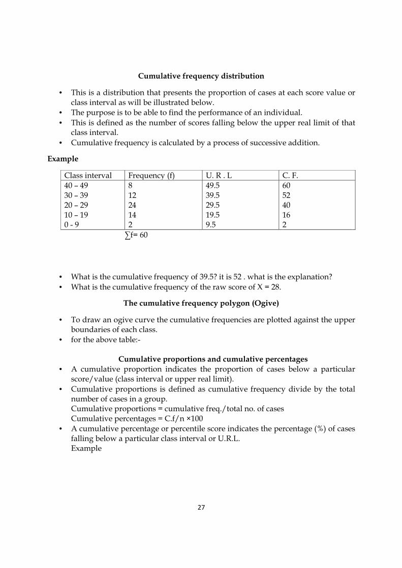
Cumulative frequency distribution

• This is a distribution that presents the proportion of cases at each score value or class interval as will be illustrated below.

• The purpose is to be able to find the performance of an individual. • This is defined as the number of scores falling below the upper real limit of that

class interval. • Cumulative frequency is calculated by a process of successive addition.

Example

Class interval Frequency (f) U. R . L C. F. 40 – 49 30 – 39 20 – 29 10 – 19 0 - 9

8 12 24 14 2

49.5 39.5 29.5 19.5 9.5

60 52 40 16 2

∑f= 60

• What is the cumulative frequency of 39.5? it is 52 . what is the explanation? • What is the cumulative frequency of the raw score of X = 28.

The cumulative frequency polygon (Ogive)

• To draw an ogive curve the cumulative frequencies are plotted against the upper boundaries of each class.

• for the above table:-

Cumulative proportions and cumulative percentages

• A cumulative proportion indicates the proportion of cases below a particular score/value (class interval or upper real limit).

• Cumulative proportions is defined as cumulative frequency divide by the total number of cases in a group. Cumulative proportions = cumulative freq./total no. of cases Cumulative percentages = C.f/n ×100

• A cumulative percentage or percentile score indicates the percentage (%) of cases falling below a particular class interval or U.R.L. Example

28

Cumulative proportion polygon and cumulative percentages polygon

• A cumulative proportions polygon is obtained by plotting the cumulative proportions against the upper real limits.

• A cumulative percentages polygon is obtained by plotting the C% against the U.R.L. The graph of Cumulative proportion polygon.

• What is the percentile equivalent of a raw of 118 in the distribution above ? P=87%+/- 1

• What is the cut-off score to select 25% and 30% of the candidates to attempt a competitive programme in the above score distribution. % equivalent of 70%=111 marks. Graph of cumulative percentages polygon.

PERCENTILE RANK

• A percentile rank is a number that indicates the percentage of scores that are equal to or less than a specified score.

• For example, if you made a score of 165 on a psychology test and this corresponds to a percentile rank of 88% of the people taking the test made a score equal or less than your score and 12% of the people taking the same test made a score greater than yours. Percentile rank=cumulative freq./freq ×100 = 23/40 × 100 = 58%.

• This means 58% of the people taking the test received a score equal to or less than 109.5.

• A much simpler procedure for calculating a percentile rank is to use the following formula: Percentile rank = (cful – (X – Xll)/n × fi ) 100 N Where:- Cful – Cumulative freq. of the upper real limits of the interval below the one containing the score of interest. X – Score of interest XLL – lower real limits fi - frequency of the interval containing X (score of interest). n – Total no. of cases i – Class size What is the percentile rank of a raw score of X=122 in the above distribution. The interval is 120 – 124. XLL =119.5. fi =4, Cful = 33 C= 5 n = 40.

29

P122 = (33 + (122 – 119.5)/5 × 4) 40 ×100 = 87.5%. How to determine a raw score given a percentile rank.

• First convert the percentile into C.F. using the following formula Percentile rank = c.f./n × 100 c.f. = (perc. Rank × no.)/100.

• Make c.f. the subject • Using the following formula calculate the cut-off score using the following

formula. X = Xll + i(c.f. – c.ful)/fi.

Example

• What is the cut-off score to select 25% of the candidates to enter into a competitive program. The percentile rank = c.f./n × 100 -The equivalent to a cut-off score of 75%. C.F. = (75 × 40)/100 = 30. Class interval f URL C.F. C.Prop. C% 115 – 119 4 119.5 30 0.83 83

• Class interval 115 – 119 has a what cut-off score XLL =114.5, fi =4, Cful =29, i= 5 Cut-off score =X=114.5 + 5(30 – 29)/4. =114.5 + 1.25 = 115.75.

Measures of central tendency

• Measures of central tendency give the researcher a convenient way of describing a set of data with a single number.

• The number, which results from computation of a measure of central tendency, represents the average or typical score attained by a group of subjects.

• The central tendency of a distribution describes the location of a centre of a distribution by indicating one score value which represents the average score.

• The three most frequently encountered indices of central tendency are; 1. Mode 2. Median 3. Mean • Each of these indices is appropriate for a different scale of measurement; • the mode is appropriate for nominal data, • the median for ordinal data, • And the mean for interval or ratio data. • Since most measurements in educational research represent an interval scale, the

mean is the most frequently used measure of central tendency.

30

Mode

• It is the most frequent, most popular and most repeated score in a distribution of scores.

• If you want to identify the modal score, you merely identify the score that occurred most frequently.

• This is the score that is attained by more subjects than any other. • The mode is not established through calculation; it is determined by looking at

the scores and seeing which score occurs most frequently. Characteristics of the mode.

• It is very simple to determine • A set of scores may have two or more modes, in which case it is referred to as

bimodal. • It is an unstable measure of central tendency • It is a poor measure of a grouped data e.g., the idea of modal class; mid-point. • It’s a poor measure of central tendency when the distribution is rectangular. • When nominal data is involved however, the mode is the only appropriate

measure of central tendency. • It is also used with multimodal distributions because the mode is the only

measure of central tendency that communicates that two distinct scores exist within the overall distribution of scores.

Limitations of the mode.

• A set of scores may have two or more modes. • Its unstable measure of central tendency because equal sized samples randomly

collected from the same population are likely to have different modes. • It’s only suitable for nominal date.

The median

• The median is useful when the exact mid-point of the data is required. • It is that point in a distribution above and below which are 50% of the scores. • It is the 50th percentile • It divides a distribution of scores exactly half way so that 50% of the scores fall

below the median and 50% of the scores fall above the median. • Consequently the median corresponds to the second quartile, Q2- that is, it

represents the 50th percentile score. • The median is the most preferred measure of central tendency with drastically

skewed distributions. Calculation of the median

• There are two methods of arriving at the median. 1. Inspection method-direct –finite 2. Formula method

Inspection method-direct –finite

• To compute the median by the direct method, we must first determine whether the group of numbers contains an even or odd number of scores.

31

• If n is odd the median is that score value that corresponds to the middle score when the scores are arranged in an ascending order. e.g., X= 2, 6, 11, 18, 29, 30, 33. N=7; the median = 18

• If n is an even no. the median is the score value falling half-way between the score of the two middle scores. Median = ((n/2)th + (n/2 + 1)th )2 E.g., compute the median of X=3, 5, 7, 8, 9, 11, 14, 16. Median = ((8/2)th + (8/2 + 1)th)/2 = (4th + 5th)/2 = (8 + 9)/2 = 17/2 = 8.5

Formulae method

• When the median is calculated from a grouped frequency distribution, the following general formula is used. Median = XLL + i(c.f.50 – c.f.ul)fc Example Calculate the median for the following frequencies.

Class interval Frequency (f) c.f. 125 – 129 120 – 124 115 – 119 110 – 114 105 – 109 100 – 104 95 – 99

3 4 4 6 8 8 7

40 37 33 29 23 15 7

Median= Cf50 = (50 ×n)100 = (50 × 40)/100 = 20. The median class = n/2 = 40/2 = 20th –c.f. Therefore, the class interval 105 – 109 has the median class. Using the median = XLL + i(c.f.50 – c.f.ul)fc

XLL = 104.5, i= 5, c.f.50 = 20, c.f.ul = 15, fc = 8. = 104.5 + 5(20 – 15)/8 =104.5 + 5(5)/8 =104.5 + 25/8 = 107.6

Characteristics of the median.

1. The median is a desirable measure of central tendency for two reasons; • It’s insensitive to extreme scores (i.e. the higher and lower scores)

E.g. income of employees are argued out by trade unions using the median, as the government base on the mean

32

• It’s not sensitive to missing scores. 2. The most reported in research.

Mean

• This is the average of the scores . • It’s the sum total of all scores, divided by the number of scores entered.

Mean (X) = ∑X/n Or X = ∑fX/∑f Where; X = arithmetic mean ∑=sum of all scores F= frequency N= number of scores.

Characteristics of the mean.

• The mean is biased or takes account of each and every score, unlike the median, it is definitely affected by extreme scores.

• It acts like a balancing point. • It is influenced by extreme scores i.e., scores that are not like other e.g., skewed

distributions. Example. Calculate the mean scored by students X and Y. X= 15, 10, 8, 6, 5, 4. Y= 60, 10, 8, 6, 5, 4. X= ∑x/n = 48/6 = 8. Y= ∑y/n = 93/6 = 15.5 The mean is not a good measure/option of skewed distributions. Properties of the mean

• The sum of the deviations from the mean will always be zero. Deviations (d) = x – x = ∑(x – x ) = 0.

• The sum of the square deviations of each score from the mean is less than the sum of square deviations about any other number. ∑(X-X)2 is minimum.

Measures of dispersion/variability

• Although measures of central tendency are useful statistics for describing a set of data, they are not sufficient.

• Two sets of data, which are very different, can have identical means or medians. • As an example consider the following sets of data

Set A- 79, 79, 79, 80, 81, 81, 81. leptokurtic Set B- 50, 60, 70, 80, 90, 100, 110.-mesokurtic

33

The means of both sets is 80 and the median of both is 80. But set A is very different from set B. In set A the scores are all very close together and clustered around the mean. In set B the scores are much more spread out; there is much more variation or variability in set B. Thus there is a need for a measure, which indicates how spread out the scores are.

• The greater the differences between the scores and by different people the spread out or scattered the scores are in the distribution. This distribution is referred to as heterogeneous.

• The smaller the difference between scores and by different people the more clustered together the scores are in the distribution. This is a homogeneous distribution, implying uniform ability. Hence a small measure of variability.

• There are a number of descriptive statistics that serves this purpose and they are referred to as a measure of variability. These are;-

1. Range 2. Semi-interquartile range 3. Mean deviation 4. Variance 5. Standard deviation

Range

• The range is simply the difference between the highest and the lowest score in a distribution and is determined by subtraction.

• It’s the distance between the highest score and the lowest score in the distribution.

• It is the crudest measure of variability, or dispersion of a group of scores. Range = highest score – the lowest score. R = Xh – Xl

Characteristics

• It uses only two extreme scores in a distribution. • The range is very unstable as it is based on two extreme scores. • The range doesn’t provide the correct pattern of variation • The range is only useful as a quick and rough estimate of measures of variability. • It is extremely unstable and is affected by chance factor

Semi-interquartile range

• To overcome the instability inherent in the range as a measure of variability the semi-interquartile range is sometimes used.

• The SIQR is half the distance between the first quartile (Q1) and the third quartile (Q3).

• SIQR is defined as half the difference between the 75th and 25th percentile score. SIQR= (Q3 – Q1)/2

34

Where; Q1 - score at 25th percentile Q3 - score at 75th percentile

• Specifically SQIR provides a measure of the spread of the middle 50% of the scores. Graphical illustration.

Characteristics

• Used with skewed distribution • It’s a measure of spread of the middle 50% of the scores • Uses two scores only • Extreme scores do not influence; hence is more stable than the range. • It is used along with the median.

Example

Calculate the semi-interquartile range for the following raw scores.

2, 3, 3, 3, 4, 4, 5, 5, 5, 5, 5, 5, 6, 6, 6, 6, 7, 7, 7, 7, 8, 8, 8, 9, 9, 9, 10, 10.

Q1 = ¼ × 28 = 7th score.

Counting the 7th score from the lowest = 5.

Q3 = ¾ × 28 = 21st score

Counting from the lowest- the largest score is 8.

Therefore, SIQR= (Q3 – Q1)/2 = ½(8 – 5) = 1.5

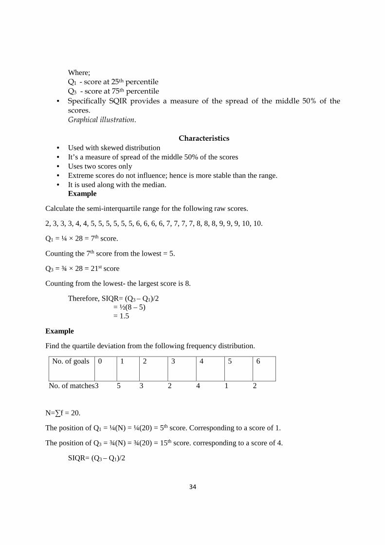
Example

Find the quartile deviation from the following frequency distribution.

No. of goals 0 1 2 3 4 5 6

No. of matches3 5 3 2 4 1 2

N=∑f = 20.

The position of Q1 = ¼(N) = ¼(20) = 5th score. Corresponding to a score of 1.

The position of Q3 = ¾(N) = ¾(20) = 15th score. corresponding to a score of 4.

SIQR= (Q3 – Q1)/2

35

=(4 – 1)/2

=1.5.

Example

Estimate the lower and the upper quartiles for the following frequency distributions by calculation.

Class interval Frequency (f) c.f. 125 – 129 120 – 124 115 – 119 110 – 114 105 – 109 100 – 104 95 - 99

3 4 4 6 8 8 7

40 37 33 29 23 15 7

Estimate the position of the lower quartile (Q1). Q1 = 1/4 (40) = 10 Q1 is therefore found within the class interval 100 – 104. Q1 = XLL + i(c.f.25 + c.f.ul)/fc XLL = 99.5, fc = 8, c.f.ul = 7, i=5, c.f.25= 10 Median = 99.5 + 5/8(10-7) = 101.38. Estimate the position of the upper quartile (Q3) on the table above. Q3 = ¾(40) = 30 Q3 is therefore, found within the intervals 115 – 119. Q3 = XLL + i(c.f.75 + c.f.ul)/fc

XLL = 114.5, fc = 4, c.f.ul = 29, i=5, c.f.75= 30 Q3 =114.5 + 5/4(30 – 29) = 115.75 SIQR= (Q3 – Q1)/2 = ½(101.38. - 115.75) = 7. 19. Mean deviation.

• We require a measure of dispersion which involves all the measures of the distribution.

• One such measure is the mean deviation. • Deviation-is the distance of a raw score from the mean.

d= X – X ∑d = ∑(X – X) = 0. NB: read about mean absolute deviations and mean squared deviations.

• Mean deviation is defined as the sum of absolute deviations divided by the total number of cases.

36

Mean deviation = ∑|X - X|/n .

Merits

• It is easy to calculate

Demerits

• Not mathematically tractable • Not useful with inferential statistics

Variance

• Variance –it is defined as the average of the sum of the squared deviations of the scores about the mean.

• The variance gives the measure of dispersion in square units. • The definitional formula for variance

S2 = ∑(X – X)2/n-1 Or S2 = ∑X2/n – 1. We often use the unbiased formula because we are not making inferences. S2 = ∑(X – X)2/n-1 The biased formula is S2 = ∑(X – X)2/n – is used while making inferences.

How to obtain the variance

Steps

• Compute the mean of the scores -(X). • Subtract the mean from each score -(X – X) • Get the difference called deviations –(d or X). • Square the deviations –(d2 or X2) • Sum the squared deviations -∑(X – X)2 • Divide the sum by the number of scores less one – (N – 1).

Merits

• It can be partitioned into different portions and the different portions attributed to different sources.

• It is unbiased • It is mathematically tractable • It can be used with inferential statistics.

37

Demerits

• It is inflated as each score is squared. • Not used with skewed distributions

Example

Calculate the variance for the following score distribution.

1, 2, 3, 7, 8, 9. Use the definitional formulae to compute the variance of the number of miles jogged daily for six consecutive days.

X X(d) X – X=X (X – X)2 = X2

1

2

3

7

8

9

5

5

5

5

5

5

-4

-3

-2

2

3

4

16

9

4

4

9

16

∑f = 30 ∑X = 0 ∑X2= 58

X = 30/6 = 5

S2 = ∑(X – X)2/n-1

= 58/5

=11.6.

The standard deviation

• Although the variance has several advantages as a measure of variability it does seem to be an inflated measure because each deviation score is squared before it is summed.

• In the example above the variance is 11.6 and the largest score is 9. • One way to avoid this inflation of the variance as an index of variability would

be to undo the squaring process that was used to circumvent the deviation scores from summing to zero.

• Standard deviation- is merely the square root of the variance. S = √∑(X – X)2/n – 1 - the unbiased formula.

38

Or S = √∑X2/n – 1

• It is used to indicate the spread, or scatter or variability that exists in a distribution of scores.

• It is affected by the spread of the scores around the mean. • The smaller the standard deviation the more homogeneous the scores are and

vice versa.

Merits

• It is unbiased • It is mathematically tractable • It can be used with inferential statistics. • It is consistent and efficient • It is the most preferred measure of variability

Demerits

• Not used with skewed distributions. • It is affected by the spread of scores from the mean.

Example

Calculate the variance and standard deviation of the following distributions.

X X – X (X – X)2

20

18

16

15

10

5

6

4

1

-2

-4

-9

36

16

1

4

16

81

∑X= 84 0 ∑(X – X)2=154

Mean (X) = ∑X/n =84/6 = 14

Variance = ∑(X – X)2/n – 1

39

= 154/6 – 1

= 30.5

Standard deviation = √variance =√∑(X – X)2/n – 1 = √154/5 = 5.55

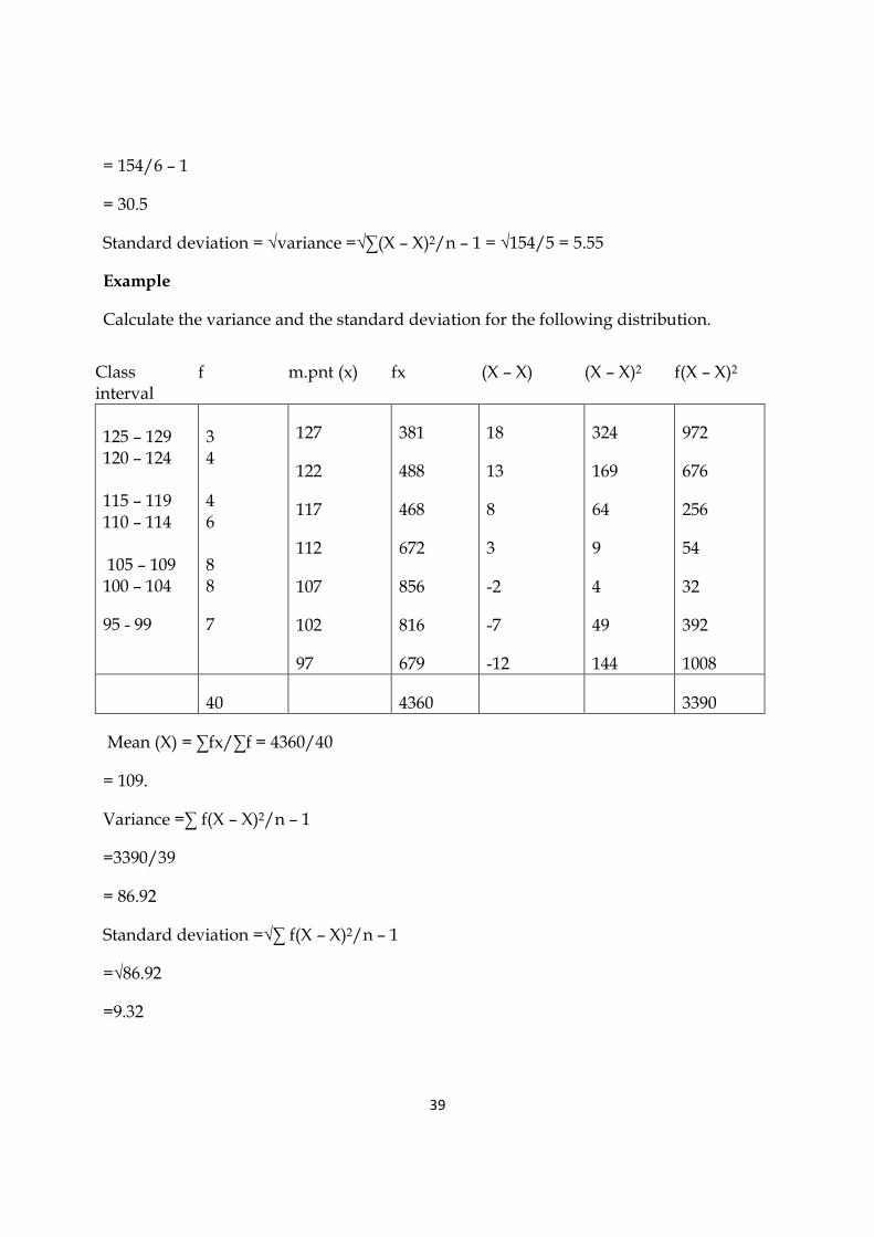
Example

Calculate the variance and the standard deviation for the following distribution.

Class interval

f m.pnt (x) fx (X – X) (X – X)2 f(X – X)2

125 – 129 120 – 124 115 – 119 110 – 114 105 – 109 100 – 104

95 - 99

3 4 4 6 8 8

7

127

122

117

112

107

102

97

381

488

468

672

856

816

679

18

13

8

3

-2

-7

-12

324

169

64

9

4

49

144

972

676

256

54

32

392

1008

40 4360 3390

Mean (X) = ∑fx/∑f = 4360/40

= 109.

Variance =∑ f(X – X)2/n – 1

=3390/39

= 86.92

Standard deviation =√∑ f(X – X)2/n – 1

=√86.92

=9.32

40

RAW SCORE FORMULAE

The variance and standard deviations of raw scores can be arrived at using the following formulae.

The variance = S2 = (∑X2 – (∑X)/n)/n-1

The standard deviation= S = √ (∑X2 – (∑X)/n)/n-1.

Example

Using the raw score formulae calculate the variance and the standard deviation in the distribution below.

Score (X) X2

20

18

16

15

10

5

400

324

225

256

100

25

∑X = 84 ∑X2 = 1330

Variance = (∑X2 – (∑X)/n)/n-1

= (1330 – (84)2/6)/5

= (1330 – 1176)/5

= 154/5

=30.8

Standard deviation = √30.8 = 5.55

41

STANDARD SCORES

• A standard score is a score that indicates how far a raw score deviates from the mean in standard deviation units.

• It is a measure of relative position which is appropriate when the data represent an interval or ratio scale.

• In behavioral research, many different scales of measurement are used to measure the outcome of a study e.g., reaction times may be measured in seconds or even milliseconds; a research questionnaire may have 50 questions or less and may have a mean of 15 with a standard deviation of 8.

• Our objective is to make comparison • To compare two characteristics measured on every person. • Therefore, different tests or measurements result in scores with varying means

and standard deviations. • Hence raw scores don’t mean much and can’t be compared directly. • However, researchers, or educators often are interested in seeing how one

person’s score compares with another. • To do this, researchers often convert raw scores into derived scores. • Derived scores are raw scores that have been translated into more useful scores

on some type of standardized basis and they include:- 1. Age and grade equivalent scores 2. Percentile ranks 3. Standard scores.

• Derived scores indicate where a particular raw score falls in relation to all other raw scores in the same distribution.

• Derived scores enable the researcher to say how well the individual has performed compared to all others taking the same test.

• Standard scores provide a means of comparing an individual’s performance relative to that of the group.

• Standard scores are also used to evaluate an individual’s performance in different instruments or subjects.

• Standard scores use a common scale to indicate how an individual compares to other individuals in the group.

• Standard scores indicate how far a given raw score is from the reference point. • Standard scores include:-

1. Z-scores 2. T-scores 3. Stanine scores 4. Percentile ranks.

• Percentiles: These scores show how a student's performance compares to others tested during test development. A student who scores at the 50th percentile performed at least as well as 50 percent of students his age in the development of

42

the test. As you will note on the table below, a score at the 50th percentile is within the average range.

• Z-Scores: These scores range from +4 to -4 and have an average of zero. Positive scores are above average. Negative scores are below average. The table below shows the approximate percentile scores that correspond to z-scores.

• T-Scores: have an average of 50 and a standard deviation of 10. Scores above 50 are above average. Scores below 50 are below average. The table below shows the approximate standard scores, percentile scores, and z-scores, scores that correspond to t-scores.

• Stanine Scores: Stanine is a contraction of the term "standard nine." These scores range from one to nine and have an average of about 4.5.

• As you can see from the table, standardized test scores enable us to compare a student's performance on different types of tests. Although all test scores should be considered estimates, some are more precise than others. Standard scores and percentiles, for example, define a student's performance with more precision than do t-scores, z-scores, or stanines

Z-SCORES

• A Z-score is the distance of a raw score from the mean in s.d. units. • One standard score that is used very frequently is a Z-score. • A Z-score expresses how far a score is from the mean in terms of standard

deviation units. • Z-scores are the simplest form of standard scores • Z-scores have the advantage that raw scores on different tests can be compared

directly. • For example, suppose a student received a score of 60 on a biology test and 80 on

a chemistry test, in which test is the student good? • A naïve observer might be endeared to infer at a glance that the student is doing

better in chemistry than in biology. • However, how well the student is doing comparatively cannot be determined

until we know the mean and standard deviations for each distribution of scores, i.e., raw scores doesn’t mean much.

• Suppose we find that biology test has a mean of 50 and s.d. of 5 and chemistry test has a mean of 90 and s.d. of 10. Now what does this tell us?

• The student’s raw score in biology is actually two standard deviations above the mean (a Z of +2); whereas his raw score in chemistry (80) is one standard deviation below the mean (a Z of -1.0).

• Therefore, a Z-score tells how many s.d. a raw score falls above or below the mean.

• Algebraically the Z-score is represented as follows. Formulae for a Z-score

43

Z = (raw score – mean)/standard deviation. =(X – X)/s.d.

Example

Peter received a score of 70 on a geography test with a mean of 50 and s.d. of 20. He also received a score of 80 in math’s test with a mean of 90 and a s.d. of 10. In which exam did peter perform better?

Solution

Geography: - X≈ (50, 20), and X = 70.

Zs = (Xs – Xs)/s.d.

Z= (70 – 50)/20 = +1.0

Maths;

X≈ (90, 10), X= 80.

Zs = (Xs – Xs)/s.d.

= (80 – 90)/10

= -1.0

• Therefore, peter’s performance in geography is better than his performance in maths.

• Peter’s score in geography is one standard deviation above the mean whereas his performance in maths is one standard deviation below the mean.

Characteristics of Z-scores

• A Z-score contains four important pieces of information about the corresponding observed or raw score.

1. The magnitude of the Z-score tells or indicates how many standard deviations a raw score lies away from the mean.

2. The sign of the Z-score indicates whether the raw score lies above the mean (Z is positive) or below the mean (Z is negative).

3. The mean of the distribution of Z-scores will always be zero regardless of the value of the original mean. Z = (∑Z)/n = 1/n (∑(X – X)/s.d. But (∑(X – X) = 0 ∑ = 1/n.s.d. (∑(X – X) =0 The mean is zero because the mean is a balancing point of a distribution.

44

4. The variance of a Z-distribution is 1.0 5. A normal distribution with a mean of 0 and a standard deviation of 1.0 is

called the standard normal distribution and it is used in the process of score interpretation or inferences.

6. Although transforming raw scores to Z-scores changes the mean and s.d. , this transformation does not alter the shape of it. The frequency of Z-scores is exactly equal to the frequency of its corresponding raw (X) score, i.e., the shape is invariant.

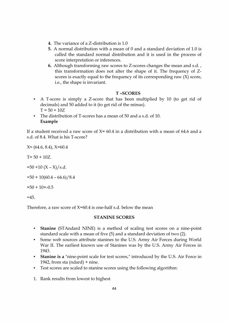
T –SCORES

• A T-score is simply a Z-score that has been multiplied by 10 (to get rid of decimals) and 50 added to it (to get rid of the minus). T = 50 + 10Z

• The distribution of T-scores has a mean of 50 and a s.d. of 10. Example

If a student received a raw score of X= 60.4 in a distribution with a mean of 64.6 and a s.d. of 8.4. What is his T-score?

X≈ (64.6, 8.4), X=60.4

T= 50 + 10Z.

=50 +10 (X – X)/s.d.

=50 + 10(60.4 – 64.6)/8.4

=50 + 10×-0.5

=45.

Therefore, a raw score of X=60.4 is one-half s.d. below the mean

STANINE SCORES

• Stanine (STAndard NINE) is a method of scaling test scores on a nine-point standard scale with a mean of five (5) and a standard deviation of two (2).

• Some web sources attribute stanines to the U.S. Army Air Forces during World War II. The earliest known use of Stanines was by the U.S. Army Air Forces in 1943.

• Stanine is a "nine-point scale for test scores," introduced by the U.S. Air Force in 1942, from sta (ndard) + nine.

• Test scores are scaled to stanine scores using the following algorithm:

1. Rank results from lowest to highest

45

2. Give the lowest 4% a stanine of 1, the next 7% a stanine of 2, etc., according to the following table:

Calculating Stanines

Result Ranking

4% 7% 12% 17% 20% 17% 12% 7% 4%

Stanine 1 2 3 4 5 6 7 8 9

• The underlying basis for obtaining stanines is that a normal distribution is divided into nine intervals, each of which has a width of 0.5 standard deviations excluding the first and last. The mean lies at the centre of the fifth interval.

• Stanines can be used to convert any test score into a single digit number. This was valuable when paper punch cards were the standard method of storing this kind of information. However, because all stanines are integers, two scores in a single stanine are sometimes further apart than two scores in adjacent stanines. This reduces their value.

• Today stanines are mostly used in educational assessment. • A statine therefore, is a standard score based on dividing the normal curve into

nine intervals along the base line. • Indeed, its very name, stanine is formed by combining the sta of standard and

nine. • We determine an individual’s stanine by identifying the percentile to which a

person’s raw score would be equivalent, and then using percentages given in the above figure, we locate the proper stanine.

• For example, if Irene earned a raw score equivalent to a 33rd percentile, then we would know that Irene’s score was in the middle of the fourth stanine (4+7+12+17 =40); and so we would assign her a stanine score of four.

• Note that with the exception of the first and ninth stanines, all of the stanines are of identical size, namely, one-half standard deviation unit.

• 99.9% of all scores are within -3 to +3 s.d. • The middle stanines extends plus and minus one-fourth (0.25) standard

deviation units from the mean.

46

THE NORMAL CURVE

• The normal distribution is a widely used statistical tool.

• The normal distribution is often referred to as a bell curve, given its bell-type shape and perfect symmetry.

• The normal curve represents a distribution of individuals and generally indicates that most individuals are typical or normal on a particular measurement, but some individuals differ from that norm; as one moves further and further away from the center of the normal curve, individuals tend to exhibit characteristics that are more atypical of the norm.

• A curious thing happens when data is summarized in a frequency distribution polygon. Regardless of the characteristics being measured (e.g., achievement, personality, height e.t.c.,) often this frequency polygon looks like a bell and so it is described as a bell-shaped curve.

• The curve is roughly symmetric, with the most frequently earned scores at the middle of the distribution and the least earned scores at the extreme of the distribution.

• The mean, mode and median provide about the same numerical values as measures of central tendency of this distribution.

• However, a normal distribution is a mathematical idealization of a particular type of symmetrical distribution; but it is a good mathematical curve that provides a good model of relative frequency distribution found in behavioural research.

• Therefore, the normal curve is the most important of all frequency polygons because any data from any variable describes a normal curve e.g., height, weight…, the normal curve is also a useful with inferential statistics as a probability distribution.

Properties of the Normal Distribution

1. Unimodal (one mode) - this implies that in a large frequency distribution then most frequently observed score X, is that value of X falling exactly at the mean of the distribution. The greater the distance between X and the mean, the smaller the frequency with which X occurs; hence the characteristic of the bell shaped.

2. Symmetrical (left and right halves are mirror images)-- just as many people above the mean as below the mean-

If the normal curve is folded about its mean, the two halves will be mirror images of each other. Therefore, the percentage of scores above the mean equals the percentage of scores below the mean.

3. Bell shaped (maximum height (mode) at the mean)

47

4. Mean, Mode, and Median are all located in the center-they are equal. 5. Asymptotic (the further the curve goes from the mean, the closer it gets to the X

axis; but the curve never touches the X axis) –the normal curve is continuous for all values of X from -∞ to +∞ ; but never touches the abscissa.

AREA UNDER the NORMAL CURVE

• 68% of our subjects are plus or minus one standard deviation • 95.4% of our subjects are plus or minus two standard deviations • 99.7% of our subjects are plus or minus three standard deviations

MEASURES USED TO ASSESS NORMALCY

• Although the normal distribution is often what people expect to see, many distributions turn out not to look exactly like a perfect bell curve. There are a number of criteria that can be used to assess the normality of a curve. The criteria often provide information regarding how much a particular distribution differs from a normal distribution.

• First, distributions can be skewed. A distribution is skewed when the mean of a sample differs from the median. When the mean exceeds the median, a distribution will be positively skewed, or skewed to the right; when the mean is less than the median, the distribution will be negatively skewed, or skewed to the left.

• A skewed distribution is one that contains extreme scores at either end of the distribution; this causes one tail of the curve to look as if it is stretched outward. For example, if a researcher examined a distribution of family income in a particular neighborhood where a billionaire lived, then the distribution would be positively skewed, because this one extremely high income would affect the shape of the distribution by literally pulling the distribution to the right by affecting the mean.

• Statisticians often indicate the level of skewness with a numerical value; a curve with a skewness of zero is a perfect normal distribution; in contrast, a curve with a skewness greater than or equal to ± 2.0 is quite highly skewed. A positive skewness value indicates that the distribution is skewed to the right (i.e., the mean is larger than the median), whereas a negative skewness value indicates that the distribution is skewed to the left (i.e., the mean is smaller than the median).

• Second, distributions also can be described in terms of their kurtosis. The term kurtosis refers to how flat or peaked a curve is. In terms of kurtosis, the normal curve is mesokurtic (i.e., neither too peaked nor flat). In contrast, distributions that are rather flat and have high standard deviations are referred to as platykurtic distribution, whereas distributions with a thin, tall center and a low standard deviation are referred to as leptokurtic distributions. A platykurtic

48

distribution might occur when there is a large amount of variability in a measure (e.g., scores on an achievement test in a particular school vary greatly, from some very low scores to some average scores to some very high scores); in contrast, a leptokurtic distribution might occur when there is little variability in a measure (e.g., scores on an achievement test for most students in the school were all very close to each other, with little variability).

INTERPRETATIONS OF THE NORMAL CURVE

• The normal curve is generally measured in standard deviation units, most commonly referred to as z-scores. The normal distribution has a mean z-score of zero and a standard deviation of 1.0.

• A z-score for any individual can be determined by subtracting the mean score of the distribution from the individual's specific score and then dividing by the standard deviation of the distribution.

• One of the most interesting mathematical features of the normal curve is that the percentages of scores that fall within certain areas under the curve are consistent across all normal distributions.

• Mathematically, exactly 34.13% of the area under the normal curve falls between the middle of the curve (which is also the mean, median, and mode), and one standard deviation above the mean (or one z-score above the mean); similarly, exactly 34.13% of the area under the curve also falls between the middle of the curve and one standard deviation below the mean.

• The percentage of area under the curve decreases as the number of standard deviation units one moves away from the mean increases. Thus an additional 13.59% of the area under the curve falls between both + 1 and + 2 standard deviations above the mean, and -1 and -2 standard deviations below the mean; an additional 2.15% of the area under the normal curve falls between =b 2 and ± 3 standard deviations above and below the mean (Sprinthall, 1997).

• The percentages of the area under the curve continue to remain identical on both the left and right-hand sides of the normal distribution as one proceeds up through higher standard deviations (z-scores). The exact percentage of area under the normal curve between any z-score and the mean can be determined by using a z-score table, which can be found in most introductory statistics text books.

• Normal curves are also related to percentile scores, which are commonly used by many educational practitioners. This is particularly important, because educators often need to report and interpret individual students' test scores for parents. A percentile is the point in a distribution below which a certain percentage of scores fall; thus a student who scored in the 60th percentile on an examination scored higher than 60% of the students who took that examination (this does not mean that the student correctly answered 60% of the questions on the examination). On a normal distribution, the 50th per-centile corresponds with the

49

middle of the curve, or a z-score of zero. When z-scores are positive, percentile measures will be above 50, whereas when z-scores are negative, percentile measures will be below 50.

• Some other scores that are typically used in the field of education also can be expressed in terms of normal distributions. One of these is T scores, which have a mean of 50 and a standard deviation of 10; another is a stanine score, which divides the normal distribution into nine distinct units. Thus a mean T score (50) corresponds to the 50th percentile, to a z-score of zero, and to a stanine score of 5.

AREAS UNDER THE NORMALCURVE

• The table below contains the area under the standard normal curve from 0 to z. this can be used to compute the cumulative

distribution function values for the standard normal distribution.

• The table utilizes the symmetry of the normal distribution, so what in fact is given is

• where a is the value of interest. This is demonstrated in the graph below for a = 0.5. The shaded area of the curve represents the

probability that x is between 0 and a.

This can be clarified by a few simple examples.

1. What is the probability that x is less than or equal to 1.53? Look for 1.5 in the X column, go right to the 0.03 column to find the

value 0.43699. Now add 0.5 (for the probability less than zero) to obtain the final result of 0.93699.

2. What is the probability that x is less than or equal to -1.53? For negative values, use the relationship

From the first example, this gives 1 - 0.93699 = 0.06301.

3. What is the probability that x is between -1 and 0.5? Look up the values for 0.5 (0.5 + 0.19146 = 0.69146) and -1 (1 - (0.5 +

0.34134) = 0.15866). Then subtract the results (0.69146 - 0.15866) to obtain the result 0.5328.

To use this table with a non-standard normal distribution (either the location parameter is not 0 or the scale parameter is not 1),

standardize your value by subtracting the mean and dividing the result by the standard deviation. Then look up the value for this

standardized value.

A few particularly important numbers derived from the table below, specifically numbers that are commonly used in significance tests, are summarized in the following table:

50

p 0.001 0.005 0.010 0.025 0.050 0.100

Zp -3.090 -2.576 -2.326 -1.960 -1.645 -1.282

p 0.999 0.995 0.990 0.975 0.950 0.900

Zp +3.090 +2.576 +2.326 +1.960 +1.645 +1.282

These are critical values for the normal distribution.

The standard normal curve

The table below gives the areas under the standard normal curve according to the distance on the baseline between the mean and a given Z-score. The total area under the standard normal curve is 1.0.

51

Area under the Normal Curve from 0 to X X 0.00 0.01 0.02 0.03 0.04 0.05 0.06 0.07 0.08 0.09 0.0 0.00000 0.00399 0.00798 0.01197 0.01595 0.01994 0.02392 0.02790 0.03188 0.03586 0.1 0.03983 0.04380 0.04776 0.05172 0.05567 0.05962 0.06356 0.06749 0.07142 0.07535 0.2 0.07926 0.08317 0.08706 0.09095 0.09483 0.09871 0.10257 0.10642 0.11026 0.11409 0.3 0.11791 0.12172 0.12552 0.12930 0.13307 0.13683 0.14058 0.14431 0.14803 0.15173 0.4 0.15542 0.15910 0.16276 0.16640 0.17003 0.17364 0.17724 0.18082 0.18439 0.18793 0.5 0.19146 0.19497 0.19847 0.20194 0.20540 0.20884 0.21226 0.21566 0.21904 0.22240 0.6 0.22575 0.22907 0.23237 0.23565 0.23891 0.24215 0.24537 0.24857 0.25175 0.25490 0.7 0.25804 0.26115 0.26424 0.26730 0.27035 0.27337 0.27637 0.27935 0.28230 0.28524 0.8 0.28814 0.29103 0.29389 0.29673 0.29955 0.30234 0.30511 0.30785 0.31057 0.31327 0.9 0.31594 0.31859 0.32121 0.32381 0.32639 0.32894 0.33147 0.33398 0.33646 0.33891 1.0 0.34134 0.34375 0.34614 0.34849 0.35083 0.35314 0.35543 0.35769 0.35993 0.36214 1.1 0.36433 0.36650 0.36864 0.37076 0.37286 0.37493 0.37698 0.37900 0.38100 0.38298 1.2 0.38493 0.38686 0.38877 0.39065 0.39251 0.39435 0.39617 0.39796 0.39973 0.40147 1.3 0.40320 0.40490 0.40658 0.40824 0.40988 0.41149 0.41308 0.41466 0.41621 0.41774 1.4 0.41924 0.42073 0.42220 0.42364 0.42507 0.42647 0.42785 0.42922 0.43056 0.43189 1.5 0.43319 0.43448 0.43574 0.43699 0.43822 0.43943 0.44062 0.44179 0.44295 0.44408 1.6 0.44520 0.44630 0.44738 0.44845 0.44950 0.45053 0.45154 0.45254 0.45352 0.45449 1.7 0.45543 0.45637 0.45728 0.45818 0.45907 0.45994 0.46080 0.46164 0.46246 0.46327 1.8 0.46407 0.46485 0.46562 0.46638 0.46712 0.46784 0.46856 0.46926 0.46995 0.47062 1.9 0.47128 0.47193 0.47257 0.47320 0.47381 0.47441 0.47500 0.47558 0.47615 0.47670 2.0 0.47725 0.47778 0.47831 0.47882 0.47932 0.47982 0.48030 0.48077 0.48124 0.48169 2.1 0.48214 0.48257 0.48300 0.48341 0.48382 0.48422 0.48461 0.48500 0.48537 0.48574 2.2 0.48610 0.48645 0.48679 0.48713 0.48745 0.48778 0.48809 0.48840 0.48870 0.48899 2.3 0.48928 0.48956 0.48983 0.49010 0.49036 0.49061 0.49086 0.49111 0.49134 0.49158 2.4 0.49180 0.49202 0.49224 0.49245 0.49266 0.49286 0.49305 0.49324 0.49343 0.49361 2.5 0.49379 0.49396 0.49413 0.49430 0.49446 0.49461 0.49477 0.49492 0.49506 0.49520 2.6 0.49534 0.49547 0.49560 0.49573 0.49585 0.49598 0.49609 0.49621 0.49632 0.49643 2.7 0.49653 0.49664 0.49674 0.49683 0.49693 0.49702 0.49711 0.49720 0.49728 0.49736 2.8 0.49744 0.49752 0.49760 0.49767 0.49774 0.49781 0.49788 0.49795 0.49801 0.49807 2.9 0.49813 0.49819 0.49825 0.49831 0.49836 0.49841 0.49846 0.49851 0.49856 0.49861 3.0 0.49865 0.49869 0.49874 0.49878 0.49882 0.49886 0.49889 0.49893 0.49896 0.49900 3.1 0.49903 0.49906 0.49910 0.49913 0.49916 0.49918 0.49921 0.49924 0.49926 0.49929 3.2 0.49931 0.49934 0.49936 0.49938 0.49940 0.49942 0.49944 0.49946 0.49948 0.49950 3.3 0.49952 0.49953 0.49955 0.49957 0.49958 0.49960 0.49961 0.49962 0.49964 0.49965 3.4 0.49966 0.49968 0.49969 0.49970 0.49971 0.49972 0.49973 0.49974 0.49975 0.49976 3.5 0.49977 0.49978 0.49978 0.49979 0.49980 0.49981 0.49981 0.49982 0.49983 0.49983 3.6 0.49984 0.49985 0.49985 0.49986 0.49986 0.49987 0.49987 0.49988 0.49988 0.49989 3.7 0.49989 0.49990 0.49990 0.49990 0.49991 0.49991 0.49992 0.49992 0.49992 0.49992 3.8 0.49993 0.49993 0.49993 0.49994 0.49994 0.49994 0.49994 0.49995 0.49995 0.49995 3.9 0.49995 0.49995 0.49996 0.49996 0.49996 0.49996 0.49996 0.49996 0.49997 0.49997 4.0 0.49997 0.49997 0.49997 0.49997 0.49997 0.49997 0.49998 0.49998 0.49998 0.49998

• The mathematical model of normal distributions defines a family of distributions. These normal distributions may differ in their means and s.d., but they all have properties of the normal curve in common.

• Since these distributions resemble each other in terms of their properties, they are often referred as a family of normal distributions.

• The normal curve permits the interpretations of scores with reference to where they fall in the distribution.

• Since 100% (a proportion of 1.00) represents an entire quantity, the total area underneath the curve of any distribution is 100% or 1.00.

• Infact the area under the relative frequency polygon is always 1.0 (trapezoidal method, Simpsons or integration can be used).

52

• Whan area is divided into parts as illustrated in the figure above, the relative frequency or proportions or percentages of scores falling in some parts of the distribution can be determined.

• However, the interpretation of scores using the above figure is of limited usefulness because Z-scores may take values other than just whole numbers.

• For this reason, a table has been made that gives the proportions of area under the standard normal curve that corresponds to each possible Z-score.

• Several questions can be answered using the Z-scores and the normal curve table.

1. What percentage of scores fall between the mean and a given raw score:- Steps

• First convert the raw score into a Z-score. • Next draw the normal curve and shade the required area. • Next read off the required area from the normal table.

Example

What is the proportion of area between Charles’ score of 70 and the mean in a distribution with a mean of 50 and s.d. of 10.

Soln.

X= 70 ≈ (50, 10)

Z = (X – X)/s.d. = (70 – 50)/10

=+2.0

From the normal table; A= 0.477.

Therefore, the proportion of scores between the mean and charles’ scores is 0.477.

Example

Suppose john earned a score of 30 in a distribution with a mean of 50 and a s.d. of 10. What proportion of scores fall between john’s score and the mean.

Soln.

X= 30 ≈ (50, 10)

Z = (X – X)/s.d = (30 – 50)/10

= -2.0

A Z-score of -2.0 s.d. implies the score of 30 is 2 s.d. below the mean. However, since the normal curve is symmetrical about the mean, the area between the mean and 2 s.d.

53

below the mean is the same as the area between the mean and the 2 s.d. above the mean. Hence the proportion is 0.477

NB: you ignore the sign since the normal curve is symmetrical.

2. What proportion of scores fall above or below a given raw score. Steps

• First convert the raw scores to a Z-score • Draw the sketch of the normal curve • Shade the area you are looking for.

Example

Find the proportion of area above Rodah’s score of 60 in a distribution with a mean of 50 and s.d. of 10.0

Soln

X = 60 ≈ (50, 10)

Z =(X – X)/s.d = (60 – 50)/10

=+1.0

Area A1 from the table is 0.341

We know that the area above or below the mean is 0.500

Therefore, the required area (above) is simply the area above the mean minus the area between the mean and +1 s.d.

Required area = 0.500 – 0.341 = 0.159

Area below:

The area below +1.0 s.d. is the sum of area below the mean (0.5) and the area between the mean and +1.0 s.d.

But A1 = 0.500 and A2 = 0.341 from the table.

Area below rodah’s score = A1 + A2 = 0.500 + 0.341 = 0.841

3. What proportion of area of scores falls between two raw scores.

Steps

• Transform the two raw scores into Z-scores • Next draw a picture of the normal distribution and locate the two z-scores on the

abscissa and shade in the area between them.

54

• Then find the proportion of scores falling below or above each of the z-scores • Then subtract the smaller area from the bigger area to find the proportion of area

between them. Example

Jane has a score of X=42 and John has a score of X=60 in a distribution with a mean of 50 and s.d. of 10. Find the proportion of scores between jane’s and john’s scores.

Soln

Jane’s

X=42 ≈ (50, 10)

Z = (X – X)/s.d = (42 – 50)/10 = -0.80

Area above Jane’s score A1 + A2

But A1 = 0.288 from the table and A2= 0.500

The area above Jane’s score = 0.288 + 0.500 = 0.788

John’s

X = 60 ≈ (50, 10)

Z = (X – X)/s.d. = (60 – 50)/10 =+1.0

Area above john’s score = area above the mean – A1 = 0.500 – 0.341 =0.159

Proportion of area between Jane’s and john’s score = 0.788 – 0.159 = 0.629.

Using area below

Area below Jane’s = 0.500 - 0.288 = 0.212

John’s

Are below john’s score = A1 + A2 = 0.500 + 0.341 = 0.841

Area between Jane’s and john’s score = 0.841 – 0..212 = 0.629

4. What raw score falls above (or below) a given percentage of scores (determining of cut-off scores). Steps.

• First draw the picture of the normal curve and shade in the area to be found.(% of scores)

• Convert the given percentage to a proportion by dividing by 100.

55

• Then turn the table and find the Z-score corresponding to the shaded area of your diagram.

• Now you know the values of Z, X, and s.d., then apply the following formulae Z= (X – X)/s.d. Make X the subject X = s.d..Z + X

Example

What raw score falls above 38% of the scores in a distribution with a mean of 50 and s.d. of 10?

Soln

38% = 0.380

A1 = 0.500 – 0.380

= 0.120

The area between the mean and the score of interest is 0.120

The area of 0.120 is between the mean and Z- score of -0.3 (to the left).

X = Z.s.d. + X

= -0.3 × 10 + 50

=-3.0 + 50

= 47

Therefore, a raw score of 47 falls above 38% of the scores.

Type of Scores

Standard Score (SS) compares the student's performance with that of other children at the same age or grade level. For reference, Standard Score of 85-115 fall within normal range. Standard score of 84 or lower fall below the normal range and scores of 116 or higher fall above normal range.

The Percentile (%) Score indicates the student's performance on given test relative to the other children the same age on which the test was nor med. A score of 50% or higher is above normal range.

Stanine Score like the Standard score reflects the student's performance compared with that of other students in the age range on which the given test was normed. For reference, a stanine of 7 is above average, a stanine of 5 is average and a stanine of 3 is below average.

56

The Standard Deviation is a useful measure of the scatter of the observations is this: if the observations follow a Normal distribution, a range covered by one standard deviation above the mean and one standard deviation below it (x+1SD) includes about 68% of the observations; a range of two standard deviations above and two below (x+2SD) about 95% of the observations; and of three standard deviations above and three below (x+3SD) about 99.7% of the observations.

57

Part II

Definition of terms.

Measurement: -This is a systematic process of assigning numerical to individuals’ properties or characteristics.

Test: - This is a device that is used to obtain a measure of individuals’ behavior.

- It is a device used to measure people characteristics i.e. height, intellectual ability, etc.

Evaluation: - This is the process of determining the usefulness / value / worth of something in terms of cost, adequacy and effectiveness.

- During evaluation, a comparison of performance & objectiveness is done. - The focus of evaluation is the usefulness or value. - It doesn’t matter with the level of marks but what is the value of the

mark attained to the evaluator’s community.

Types of Tests

i) Criterion – referenced tests

These are the tests concerned with level of mastery of such defined skills (domain-referenced).

They focus solely on reaching a standard of performance on a specific skill called for by the test exercises.

The test itself and the domain of content it represents provide the standard.

Many, perhaps most assessments needed for instructional decisions are of this sort.

ii) Norm – referenced tests

This is a case where performance is evaluated not in relation to the set of tasks per se, but in relation to the performance of some more general reference group.

The quality of the performance is defined by comparison with the behavior of others.

Test of this kind may appropriately be used in many situations calling for curricular, guidance, or research decisions.

58

Types of Evaluation

a) Formative evaluation This is an evaluation given out by teachers and counselors who are often interested in using tests to determine their students’ and clients’ strengths and weaknesses, the areas where they are doing well and those where they are doing poorly.

Assessment for this purpose, guide future instruction i.e. test results are used to inform or shape the course of instruction e.g. C.A.Ts.

b) Summative evaluation An evaluation done to reach a summary statement of the person’s accomplishments to date (e.g. end of course exams, K.C.S.E., e.t.c.) and it is used for placement decisions.

It provides a summary of student achievement i.e. used after instruction is completed to summarize what students have learned.

Includes both teachers-constructed and administered tests, which are typically used to make decisions about grades, and standardized achievement tests, which are used to evaluate instruction and identify exceptionally high - or low - performing students.

Evaluation Process

Measurement is one form of evidence used during the process of evaluation. Evaluation in education involves determining the congruence between performance and learning behavior. However, tests and examinations provide evidence on performance but not learning behavior.

The process of evaluation involves the following steps:

i) Identification of a specific community ii) Specification of the community needs e.g. economic, social or political needs iii) Specification of objectives derived from community needs iv) Identification of activities people can participate in to achieve the needs v) Specification of conditions under which activities should be carried out vi) Development of instruments to measure achievement of needs vii) Stating conditions under which the instruments can best measure

achievement of the needs viii) Administration of the instrument ix) Rating the measurements and interpretation of the results x) Provision of feedback to the community.

59

Evaluation Instrument.

An evaluation instrument is any tool or device/means used to obtain measurements about the behavior or characteristics of an object or individual. In education, examples of evaluation instruments are tests and examinations.

The three main characteristics (criteria) of evaluation instruments are:

1. Reliability 2. Validity 3. Usability/Practicability.

Reliability

This is the consistency of measurements when the same instrument is administered to the same group of people more than once.

It is the ability of the instrument to accurately reproduce the same measurements/scores.

Some degree of inconsistency is present in all measurement procedures. If for example we call a given score a true score (T), then each observed score or measurement (X) includes this true score plus some error of measurement (e) i.e.

X = T + e

Any difference between an observed score (X) and the true score (T) is an error of measurement (e) i.e. e = X – T

The types of reliability evidences are:

a) Stability reliability evidence. Provide evidence about consistence of test result over a period of time e.g. test-retest method where some test is administered to the same group but different dates. Correlation co-efficient between 1st and 2nd measures is done.

b) Equivalent form reliability evidence. Provide evidence about the consistence of scores for a group of people with different tests on the same date and now calculate correlation co-efficient. The tests should be of the same ability, similar characteristics of what to test, same topic and same instructions.

c) Stability and Equivalent reliability evidence. Provide evidence on the consistence of the test performance by group of people on different tests administered in different tests administered in different dates. Then calculate correlation co-efficient.

60

d) Scorer/Marker reliability evidence. Provide evidence on the consistence on marking processes and they are done thro:

i) Inter-Scorer:- Same responses from same group of people are marked by different markers/scorers. Correlation co-efficient between 1st & 2nd scores.

ii) Intra-Scorer:- Same responses, same scorer, but the scorer has to mark the responses more than once. Then the correlation co-efficient is worked out between the two scores.

e) Internal Consistency reliability evidence. Provide evidence on contribution of each item or a set of items contribution to the final score or how a section of items related to final score.

Split-half method can be used where tests are divided into two equal halves, and each half is scored and marked independently, then correlation co-efficient for the two halves calculated. If the two halves have high correlation coefficient, it means the items between the tests are related. Low correlation or no correlation means the tests are not related, the characteristic in one half is different from the 2nd half.

Validity

Validity refers to how well the instrument measures what it is supposed to measure. It is the degree to which inferences can be made from the measurements in terms of the subject content and the learning behavior.

The types of validity evidences are:

a) Content validity evidence. Provides evidence on how well the subject content and learning behavior are reflected in the instrument. It is estimated using blue print or grid of test specification. The instrument should adequately sample the prescribed curriculum and include cognitive, affective and psychomotor domains & levels of objectives.

b) Criterion-related validity evidence.

Provides evidence on how the instrument compares with other already established instruments. They are two types, namely:

- Predictive validity evidence - Concurrent validity evidence.

61

c) Construct validity evidence. Provides evidence on how well the measurements from the instrument can be interpreted in psychological constructs e.g. intelligence, creativity, honesty, fear, innovativeness, e.t.c

Usability/Predictability

Involves the interpretation of the test scores and their use in making education related decision:-

i) Ease of interpretation and application ii) Time required for administration iii) Ease of administration iv) Cost of testing v) Ease of scoring, etc.

Ceiling Effect.

A ceiling effect is said to occur when those taking the test (or the examinees) score at or near the maximum score. This is when most of the examinees score highly. The ceiling effect performance can be illustrated using the following negatively skewed graph:

The ceiling effect may imply:

i) Poor test construction is where tasks are far much below examinees abilities i.e. task was too easy.

ii) Good teaching-learning process i.e. the teaching was well facilitated and learners were motivated to learn and led to good performance.

iii) Focus on mastery learning where most of the learners mastered the required skills.

iv) Good achievement of the educational goals/objectives by most of the learners. v) Adequate achievement of the needs of the community. vi) Good education system or programmes.

62

Floor Effect.

A floor effect is said to occur when those taking the test (examinees) score at or near the minimum score or at chance level. This is when the examinees perform very poorly. The floor effect performance can be illustrated by the following positively skewed graph:

The floor effect may imply:

- Poor test construction if the tasks are far much high compared to the level of the examinees.

- Poor teaching-learning process, that leads to poor performance. - Focus was on selection of a few individuals for specific activities,

specialized skills. - Poor or no achievement of educational goals and/or objectives by most

learners. - Poor or no achievement of the needs of the community. - Poor educational system or programmes.