ptolemy ii - eecs at uc berkeley · volume 3 ptolemy ii domains this volume describes ptolemy ii...

PTOLEMY IIHETEROGENEOUS

CONCURRENT MODELING AND DESIGN IN JAVA

Edited by:Christopher Brooks, Edward A. Lee, Xiaojun Liu, Steve Neuendorffer, Yang Zhao, Haiyang Zheng

VOLUME 3: PTOLEMY II DOMAINS

Authors:Shuvra S. BhattacharyyaChristopher BrooksElaine CheongJohn Davis, IIMudit GoelBart KienhuisEdward A. LeeJie LiuXiaojun LiuLukito MuliadiSteve NeuendorfferJohn ReekieNeil SmythJeff TsayBrian VogelWinthrop WilliamsYuhong XiongYang ZhaoHaiyang Zheng

Department of Electrical Engineering and Computer SciencesUniversity of California at Berkeleyhttp://ptolemy.eecs.berkeley.edu

Document Version 5.0for use with Ptolemy II 5.0July 15, 2005

Memorandum UCB/ERL M05/23Earlier versions:• UCB/ERL M04/17• UCB/ERL M03/29• UCB/ERL M02/23• UCB/ERL M01/12• UCB/ERL M99/40

This project is supported by the National Science Foundation (NSF award number CCR-00225610), and Chess (the Center for Hybrid and Embedded Software Systems), which receives support from NSF and the following companies: Agilent, General Motors, Hewlett-Packard,Honeywell, Infineon, and Toyota.

A

•T

HE

•UN

IVE

RS I T Y • O F • C

AL

I FO

RN

IA•

•1868•

LET THE R E BE

LIG H T

Copyright 1998-2005 The Regents of the University of California.All rights reserved.

“Java” is a registered trademark of Sun Microsystems.

VOLUME 3

PTOLEMY II DOMAINS

This volume describes Ptolemy II domains. The domains implement models of computation, which aresummarized in chapter 1. Most of these models of computation can be viewed as a framework for com-ponent-based design, where the framework defines the interaction mechanism between the compo-nents. Some of the domains (CSP, DDE, and PN) are thread-oriented, meaning that the componentsimplement Java threads. These can be viewed, therefore, as abstractions upon which to build threadedJava programs. These abstractions are much easier to use (much higher level) than the raw threads andmonitors of Java. Others (CT, DE, SDF) of the domains implement their own scheduling betweenactors, rather than relying on threads. This usual results in much more efficient execution. The Giottodomain, which addresses real-time computation, is not threaded, but has concurrency features similarto threaded domains. The FSM domain is in a category by itself, since in it, the components are notproducers and consumers of data, but rather are states. The non-threaded domains are described first,followed by FSM and Giotto, followed by the threaded domains. Within this grouping, the domains areordered alphabetically (which is an arbitrary choice).

Volume 1 is an introduction to Ptolemy II, including tutorials on use of the software, and volume 2describes the Ptolemy II software architecture.

This page intentional left mostly blank.

Contents

Volume 3

Ptolemy II Domains 3Contents 5

1. DE Domain 11.1. Introduction 1

1.1.1. Model Time 11.1.2. Simultaneous events 21.1.3. Iteration 41.1.4. Starting a Model 41.1.5. Pure Events at the Current Time 41.1.6. Stopping Execution 5

1.2. Overview of The Software Architecture 51.3. The DE Actor Library 71.4. Mutations 71.5. Writing DE Actors 9

1.5.1. General Guidelines 91.5.2. Examples 121.5.3. Thread Actors 14

1.6. Composing DE with Other Domains 151.6.1. DE inside Another Domain 161.6.2. Another Domain inside DE 18

2. CT Domain 192.1. Introduction 19

2.1.1. System Specification 212.1.2. Time 22

2.2. Solving ODEs numerically 232.2.1. Basic Notations 232.2.2. Fixed-Point Behavior 242.2.3. ODE Solvers Implemented 242.2.4. Discontinuity 262.2.5. Breakpoint ODE Solvers 27

2.3. Signal Types 272.4. CT Actors 29

2.4.1. CT Actor Interfaces 292.4.2. Actor Library 292.4.3. Domain Polymorphic Actors 32

2.5. CT Directors 332.5.1. ODE Solvers 332.5.2. CT Director Parameters 33

2.5.3. CTMultiSolverDirector 342.5.4. CTMixedSignalDirector 342.5.5. CTEmbeddedDirector 35

2.6. Interacting with Other Domains 352.7. CT Domain Demos 36

2.7.1. Lorenz System 362.7.2. Microaccelerometer with Digital Feedback. 382.7.3. Sticky Point Masses System 39

2.8. Implementation 402.8.1. ct.kernel.util package 402.8.2. ct.kernel package 412.8.3. Scheduling 452.8.4. Controlling Step Sizes 462.8.5. Mixed-Signal Execution 472.8.6. Hybrid System Execution 47

Appendix: Brief Mathematical Background 483. SDF Domain 49

3.1. Purpose of the Domain 493.2. Using SDF 49

3.2.1. Deadlock 493.2.2. Consistency of data rates 513.2.3. How many iterations? 523.2.4. Granularity 52

3.3. Properties of the SDF domain 533.3.1. Scheduling 543.3.2. Hierarchical Scheduling 553.3.3. Hierarchically Heterogeneous Models 56

3.4. Software Architecture 563.4.1. SDF Director 563.4.2. SDF Scheduler 573.4.3. SDF ports and receivers 593.4.4. ArrayFIFOQueue 60

3.5. Actors 604. FSM Domain 61

4.1. Introduction 614.2. Building FSMs in Vergil 62

4.2.1. Alternate Mark Inversion Coder 624.3. The Implementation of FSMActor 64

4.3.1. Guard Expressions 644.3.2. Actions 664.3.3. Execution 66

4.4. Modal Models 674.4.1. A Schmidt Trigger Example 674.4.2. Implementation 694.4.3. Applications 69

5. Giotto Domain 715.1. Introduction 71

5.2. Using Giotto 715.3. Interacting with Other Domains 74

5.3.1. Giotto Embedded in DE and CT 745.3.2. FSM and SDF embedded inside Giotto 75

5.4. Software structure of the Giotto Domain and implementation 765.4.1. GiottoDirector 775.4.2. GiottoScheduler 785.4.3. GiottoReceiver 795.4.4. GiottoCodeGenerator 80

6. CSP Domain 816.1. Introduction 816.2. Properties of the CSP Domain 82

6.2.1. Atomic Communication: Rendezvous 826.2.2. Choice: Nondeterministic Rendezvous 826.2.3. Deadlock 846.2.4. Time 846.2.5. Differences from Original CSP Model as Proposed by Hoare 85

6.3. Using CSP 856.3.1. Unconditional vs. Conditional Rendezvous 856.3.2. Time 87

6.4. The CSP Software Architecture 886.4.1. Class Structure 886.4.2. Starting the model 886.4.3. Detecting deadlocks: 906.4.4. Terminating the model 916.4.5. Pausing/Resuming the Model 91

6.5. Example CSP Applications 926.5.1. Dining Philosophers 926.5.2. Hardware Bus Contention 93

6.6. Technical Details 936.6.1. Rendezvous Algorithm 936.6.2. Conditional Communication Algorithm 946.6.3. Modification of Rendezvous Algorithm 98

7. DDE Domain 997.1. Introduction 997.2. Using DDE 99

7.2.1. DDEActor 1007.2.2. DDEIOPort 1007.2.3. Feedback Topologies 100

7.3. Properties of the DDE domain 1017.3.1. Enabling Communication: Advancing Time 1017.3.2. Maintaining Communication: Null Tokens 1027.3.3. Alternative Distributed Discrete Event Methods 104

7.4. The DDE Software Architecture 1057.4.1. Local Time Management 1057.4.2. Detecting Deadlock 1067.4.3. Ending Execution 106

7.5. Example DDE Applications 1078. PN Domain 109

8.1. Introduction 1098.2. Using PN 110

8.2.1. Deadlock in Feedback Loops 1108.2.2. Designing Actors 110

8.3. Properties of the PN domain 1108.3.1. Asynchronous Communication 1108.3.2. Bounded Memory Execution 1118.3.3. Time 1118.3.4. Mutations 112

8.4. The PN Software Architecture 1128.4.1. PNDirector 1128.4.2. TimedPNDirector 1128.4.3. PNQueueReceiver 1138.4.4. Handling Deadlock 1148.4.5. Finite Iterations 1148.4.6. NondeterministicMerge 114

9. PSDF Domain 1159.1. Purpose of the Domain 1159.2. Using PSDF 115

9.2.1. Restricted Reconfiguration 1169.2.2. Symbolic scheduling limitations 117

9.3. Properties of the PSDF domain 1179.3.1. Scheduling 1179.3.2. Local Synchrony and Reconfiguration Analysis 118

9.4. Software Architecture 1199.5. Actors 119

10. HDF Domain 12110.1.Introduction 12110.2.Using HDF in Vergil 121

10.2.1. Data Rates of the Modal Model 12110.2.2. Multi-Token Syntax in Guard Expressions 12210.2.3. Actions in Modal Model 123

10.3.Properties of the HDF domain 12310.3.1. Scheduling 12310.3.2. Hierarchical Heterogeneous Models 123

10.4.Software Architecture 12310.4.1. HDF Director 12310.4.2. HDFFSM Director 124

10.5.Actors 12411. DDF Domain 125

11.1.Introduction 12511.2.Properties of the DDF domain 125

11.2.1. Firing Rules 12611.2.2. Scheduling 126

11.3.Software Architecture and Implementation 12811.3.1. DDFDirector 12811.3.2. Writing DDF Actors 129

11.4.Example DDF Applications 13111.4.1. Conditionals with If-Else Structure 13111.4.2. Data-Dependent Iterations 13211.4.3. Recursion 134

References 135Index 145

Heterogeneous Concurrent Modeling an

1
DE Domain
Authors: Adam CataldoEdward A. LeeLukito MuliadiWinthrop WilliamsHaiyang Zheng

1.1 Introduction

The discrete-event (DE) domain supports time-oriented models of systems such as queueing sys-tems, communication networks, and digital hardware. In this domain, actors communicate by sendingevents, where an event is a data value (a token) and a tag, which contains a time stamp and microstep.The microstep is used to sort simultaneous events, that is, events with the same time stamp. Formally,a tag , where is a real number representing the time stamp and is natural number repre-senting the microstep.

A DE scheduler ensures that events are processed chronologically according to this time stamp byfiring those actors whose available input events are the oldest (having the earliest time stamp of allpending events). Thus, all DE actors are assumed to be causal. Informally, a DE actor is causal if anyoutput event with tag depends only on input events with tags earlier than or equal to . A tag is earlier than tag if or if and . See [27] for a mathematical definition.

A key strength in our implementation is that simultaneous events (those with identical timestamps) are handled systematically and deterministically. Another strength is that the global eventqueue uses an efficient structure that minimizes the overhead associated with maintaining a sorted listwith a large number of events.

1.1.1 Model Time

In the DE model of computation, time is global, in the sense that all actors share the same globaltime stamp and microstep. The current time and current microstep of the model are advanced by the

t τ n,( )= τ n

t t τ1 n1,( )τ2 n2,( ) τ1 τ2< τ1 τ2= n1 n2<

d Design 1

DE Domain

DE director. The current time of the model is often called the model time or simulation time to avoidconfusion with current real time.

As in most Ptolemy II domains, actors communicate by sending tokens through ports. Ports can beinput ports, output ports, or both. Tokens are sent by an output port and received by all input ports con-nected to the output port through relations. When a token is sent from an output port, it is packaged asan event and stored in a global event queue. When an actor does not specify the time stamp of an out-put, the time of the event is the model time and its microstep is the current microstep. Specialized DEactors can produce events with future time stamps. In the current implementation, only the DE directorcan advance the time stamp. Also the microstep can only be advanced by the DE director.

Actors may request that they be fired now, or at some time in the future, by calling the fireAt()method of the director. This places a pure event (one with a time stamp and a microstep, but no data)on the event queue at the time which is given as a parameter to the fireAt() method. This time must begreater than or equal to the current time. A pure event can be thought of as setting an alarm clock to beawakened in the future. Sources (actors with no inputs) are thus able to be fired despite having noinputs to trigger a firing of the whole model. Moreover, actors that introduce delay (outputs have largertime stamps than the inputs) can use this mechanism to schedule a firing in the future to produce anoutput. For convenience, the director has a fireAtCurrentTime() method, which calls fireAt() with themodel time as a parameter. This permits I/O actors to have themselves fired in real-time whenever dataarrives at a physical I/O port. When the fireAtCurrentTime() method is called, the actor will be fired atthe next microstep. Also for convenience, the director provides a fireAtRelativeTime(). Note thatfireAt() cannot take as a parameter a time earlier than the model time.

In the global event queue, events are sorted based on their tags, including time stamps andmicrosteps, and depths (explained in the next section). An event is removed from the global eventqueue when the model time reaches its time stamp, and if it has a data token, then that token is put intothe destination input port.

At any point in the execution of a model, the events stored in the global event queue have timestamps greater than or equal to the model time. The DE director is responsible for advancing (i.e.incrementing) the model time when all events with time stamps equal to the current model time havebeen processed (i.e. the global event queue only contains events with time stamps strictly greater thanthe current time). The current time is advanced to the smallest time stamp of all events in the globalevent queue.

1.1.2 Simultaneous events

An important aspect of a DE domain is the prioritizing of simultaneous events. This gives thedomain a dataflow-like behavior for events with identical tags. It is done by assigning a depth to eachactor and a microstep to each phase of execution within a given time stamp. Each depth is a non-nega-tive integer, uniquely assigned; i.e. no two actors are assigned the same depth.

The depth of an actor determines the priority of events destined to that actor, relative to otherevents with the same time stamp and the same microstep. The highest priority events are those destinedto actors with the lowest depth.

Consider the simple topology shown in figure 1.1. Assume that actor Y is not a delay actor, mean-ing that its output events have the same time stamp and microstep as its input events (this is suggestedby the dotted arrow). Suppose that actor X produces an event with time stamp . That event is avail-able at ports B and D, so the scheduler could choose to fire actors Y or Z. Which should it fire? Intu-ition tells us it should fire the upstream one first, Y, because that firing may produce another event with

τ

2 Ptolemy II

DE Domain

time stamp at port D (which is presumably a multiport). It seems logical that if actor Z is going to getone event on each input channel with the same time stamp, then it should see those events in the samefiring. Thus, if there are simultaneous events at B and D, then the one at B will have higher priority.

The depths are determined by a topological sort of a directed acyclic graph (DAG) of the actors.The DAG of actors follows the topology of the graph, except when there are declared delays. Once theDAG is constructed, it is sorted topologically. This simply means that an ordering of actors is assignedsuch that an upstream actor in the DAG is earlier in the ordering than a downstream actor. The depth ofan actor is defined to be its position in this topological sort, starting with zero. For example, in figure1.1, X will have depth 0, Y will have depth 1, and Z will have depth 2.

In general, a DAG has several correct topological sorts. The topological sort is not unique, mean-ing that the depths assigned to actors are somewhat arbitrary. But an upstream actor will always have alower depth than a downstream actor, unless there is an intervening delay actor. Thus, given simulta-neous input events with the same microstep, an upstream actor will always fire before a downstreamactor. Such a strategy ensures that the execution is deterministic, assuming the actors only communi-cate via events. In other words, even though there are several possible choices that a scheduler couldmake for an ordering of firings, all choices that respect the priorities yield the same results.

There are situations where constructing a DAG following the topology is not possible. Considerthe topology shown in figure 1.2. It is evident from the figure that the topology is not acyclic. Indeed,figure 1.2 depicts a zero-delay loop where topological sort cannot be done. The director will refuse torun the model, and will terminate with an error message.

The TimedDelay actor in DE is a domain-specific actor that asserts a delay relationship betweenits input and output. Thus, if we insert a TimedDelay actor in the loop, as shown in figure 1.3, thenconstructing the DAG becomes once again possible. The TimedDelay actor breaks the precedences.Below we will explain how you can write custom actors that have the same property.

Note in particular that the TimedDelay actor breaks the precedences even if its delay parameter isset to zero. Thus, the DE domain is perfectly capable of modeling feedback loops with zero time delay,but the model builder has to specify the order in which events should be processed by placing a Timed-Delay actor with a zero value for its parameter. Note that a time delay of 0.0 time will still advance themicrostep by one.

FIGURE 1.1. If there are simultaneous events at B and D, then the one at B will have higher priority because it may trigger another simultaneous event at D.

X A

Y CB

ZD

τ

FIGURE 1.2. An example of a directed zero-delay loop.

X C

B

AY ED

Heterogeneous Concurrent Modeling and Design 3

DE Domain

1.1.3 Iteration

At each iteration, after advancing the current tag, the director chooses all events in the global eventqueue that have the smallest time stamps, microstep, and depth (tested in that order). If two eventshave the same time stamp, microstep, and depth, they are destined to the same actor, since the depth isunique for each actor. These events are ordered by the order in which they are produced. The chosenevents are then removed from the global event queue and their data tokens are inserted into the appro-priate input ports of the destination actor. Then, the director iterates the destination actor; i.e. it invokesprefire(), fire(), and postfire(). The director will keep iterating the destination actor until there are noevents in its input ports or its prefire() method returns false.

A firing of an actor may produce additional events at the current model time and the currentmicrostep (the actor reacts instantaneously, or has zero delay), which are pending on the event queue.The DE director repeats the above procedure until there are no more events with their time stamp andmicrostep equal to the current tag. This concludes one iteration of the model. An iteration, therefore,processes all events on the event queue with the smallest tag.

1.1.4 Starting a Model

Before one of the iterations described above can be run, there have to be initial events in the globalevent queue. Actors may produce initial pure events or regular output events in their initialize()method. A model starts when at least one actor must produce events. All the domain-polymorphictimed sources described in the Actor Libraries chapter produce pure events, so these can be used inDE. We can define the start time to be the smallest time stamp of these initial events.

1.1.5 Pure Events at the Current Time

An actor calls fireAt() to schedule a pure event. The pure event is a request to the scheduler to firethe actor sometime in the future. However, the actor may choose to call fireAt() with the time argu-ment equal to the current time. In fact, the preferred method for domain-polymorphic source actors toget started is to have code like the following in their initialize() method:

Director director = getDirector();director.fireAt(this, director.getModelTime());

This will schedule a pure event on the event queue with microstep zero and depth equal to that of thecalling actor.

An actor may also call fireAt() with the current time in its fire() method. This is a request to berefired later in the current iteration. This is managed by queueing a pure event with microstep one

FIGURE 1.3. A Delay actor can be used to break a zero-delay loop.

X C

B

AY ED

Delay

IJ

4 Ptolemy II

DE Domain

greater than the current microstep. In fact, this is the only situation in which the microstep is incre-mented beyond zero.

A pure event at the current time can also be scheduled by code like the following:

Director director = getDirector();director.fireAtCurrentTime(this);

This code is equivalent to the previous example when used within standard actor methods like ini-tialize() and fire(). This is because the director never advances model time while an actor is being ini-tialized or fired. However, when methods (such as an I/O callback) queue events at the current time,they need to use the latter code. This is because the director runs in a separate thread from the callbackand, in the former code, will occasionally advance the model time between the call to getModelTime()and the call to fireAt().

1.1.6 Stopping Execution

Execution stops when one of these conditions becomes true:• The global event queue becomes empty and the stopWhenQueueIsEmpty parameter of the director

is true.• No matter whether the stopWhenQueueIsEmpty parameter is true or false, when the current model

time reaches the stop time (set by calling the setStopTime() method of the DE director) and there are no events with time stamp equal to the current model time.

Events at the stop time are processed before stopping the model execution. The execution ends by call-ing the wrapup() method of all actors. Wrapup() is called even when execution has been stopped due toan exception. Therefore, throwing an exception in the wrapup() method of an actor is not recom-mended as this exception will mask the original exception, making the source of the original exceptiondifficult to locate.

It is also possible to explicitly invoke the iterate() method of the manager for some fixed numberof iterations. Recall that an iteration processes all events with the same tag, so this will run the modelthrough a specified number of discrete time steps and microsteps.

Note that an actor can prevent execution from stopping properly if it blocks in its fire() method. Anactor which blocks in fire() should have a stopFire() method which, when called, notifies the fire()method to cease blocking and return.

1.2 Overview of The Software Architecture

The UML static structure diagram for the DE kernel package is shown in figure 1.4. For modelbuilders, the important class is DEDirector. At the heart of DEDirector is a global event queue thatsorts events according to their time stamps, microsteps, and depths (priorities).

The DEDirector uses an efficient implementation of the global event queue, a calendar queue datastructure [20]. In theory, the time complexity for this particular implementation is O(1) in bothenqueue and dequeue operations. This means that the time complexity for enqueue and dequeue oper-ations is independent of the number of pending events in the global event queue. However, to realizethis performance, it is necessary for the distribution of events to match certain assumptions. Our calen-


DE Domain

FIGURE 1.4. UML static structure diagram for the DE kernel package.

DEDirector

+DEDirector()+DEDirector(w : Workspace)+DEDirector(c : CompositeEntity, name : String)+fireAtRelativeTime(actor : Actor, time : double)+getEventQueue() : DEEventQueue+getRealStartTimeMillis() : long+getStartTime() : double+getStopTime() : double#_dequeueEvents() : Actor#_disableActor(actor : Actor)#_enqueueEvent(actor : Actor, time : double)#_enqueueEvent(rcv : DEReceiver, tk : Token, time : double)#_enqueueEvent(rcv : DEReceiver, tk : Token)#_getDepth(actor : Actor) : int

+binCountFactor : Parameter(IntToken)+isCQAdaptive : Parameter(BooleanToken)+minBinCount : Parameter(IntToken)+startTime : Parameter(DoubleToken)+stopTime : Parameter(DoubleToken)+stopWhenQueueIsEmpty : Parameter(BooleanToken)+synchronizeToRealTime : Parameter(BooleanToken)#_eventQueue : DEEventQueue#_noMoreActorsToFire : boolean#_stopRequested : boolean-_disabledActors : Set-_microstep : int

DEActor

+DEActor(container : CompositeEntity, name : String)

DEIOPort

+DEIOPort()+DEIOPort(c : ComponentEntity, name : String, isInput : boolean, isOutput : boolean)+DEIOPort(container : ComponentEntity, name : String)+DEIOPort(workspace : Workspace)+broadcast(token : Token, delay : double)+send(channelIndex : int, token : Token, delay : double) : void

Director

TypedAtomicActor

TypedIOPort

1..10..n

«Interface»DEEventQueue

+clear()+get() : DEEvent+isEmpty() : boolean+put(event : DEEvent)+take() : DEEvent

DECQEventQueue

+DECQEventQueue()+DECQEventQueue(minBinCount : int, binCountFactor : int, isAdaptive : boolean)

-_cQueue : CalendarQueue

DEEvent

+DEEvent(rc : DEReceiver, tk : Token, tStamp : double, microstep : int, depth : int)+DEEvent(actor : Actor, timeStamp : double, microstep : int, depth : int)+actor() : Actor+compareTo(event : DEEvent) : final int+depth() : int+isSimultaneousWith(event : DEEvent) : boolean+microstep() : int+receiver() : DEReceiver+timeStamp() : double+token() : Token

-_actor : Actor-_microstep : int-_receiver : DEReceiver-_receiverDepth : int-_timeStamp : double-_token : Token«Interface»

TimedActor

AbstractReceiver

«Interface»Comparable

DECQEventQueue.DECQComparator

+compare(o1 : Object, o2 : Object) : int

-_binWidth : DEEvent-_zeroReference : DEEvent

«Interface»CQComparator

«Interface»Debuggable

DEReceiver

+DEReceiver()+DEReceiver(container : IOPort)+getDirector() : DEDirector+put(token : Token, time : double)+setDelay(delay : double)#_triggerEvent(token : Token)

-_delay : double-_tokens : LinkedList

«Interface»SequenceActor

inner class

DEEDirector

6 Ptolemy II

DE Domain

dar queue implementation observes events as they are dequeued and adapts the structure of the queueaccording to their statistical properties. Nonetheless, the calendar queue structure will not prove opti-mal for all models. For extensibility, alternative implementations of the global event queue can be real-ized by implementing the DEEventQueue interface and specifying the event queue using theappropriate constructor for DEDirector.

The DEEvent class carries tokens through the event queue. It contains their time stamp, theirmicrostep, and the depth of the destination actor, as well as a reference to the destination actor. Itimplements the java.lang.Comparable interface, meaning that any two instances of DEEvent can becompared. The private inner class DECQEventQueue.DECQComparator, which is provided to the cal-endar queue at the time of its construction, performs the requisite comparisons of events.

1.3 The DE Actor Library

The DE domain has a small library of actors in the ptolemy.domains.de.lib package, shown in fig-ure 1.5. The DETransformer base class for actors provides an input and output port. The TimedDelayand Server actors influence the firing priorities as explained below by specifying function dependen-cies. The Merge actor merges events sequences in chronological order.

1.4 Mutations

The DE director tolerates changes to the model during execution. The change should be queuedusing requestChange(). While invoking those changes, the method invalidateSchedule() is expected tobe called, notifying the director that the topology it used to calculate the priorities of the actors is nolonger valid. This will result in the priorities being recalculated the next time prefire() is invoked.

An example of a mutation is shown in figures 1.6. Figure 1.7 defines a class that constructs a sim-ple model in its constructor. The model consists of a clock connected to a recorder. The method insert-Clock() creates an anonymous inner class that extends ChangeRequest1. Its execute() methoddisconnects the two existing actors, creates a new clock and a merge actor, and reconnects the actors asshown in figure 1.6.

When the insertClock() method is called, a change request is queued with the top-level compositeactor, which delegates the request to the manager. The manager executes the request after the currentiteration completes. Thus, the change will always be executed between non-equal time stamps, sincean iteration consists of processing all events at the current time stamp.

Actors that are added in the change request are automatically initialized. Note, however, one sub-tlety. The next to last line of the insertClock() method is:

_rec.input.createReceivers();

This method call is necessary because the connections of the recorder actor have changed, but since theactor is not new, it will not be reinitialized. Recall that the preinitialize() and initialize() methods are

1. Often a more convenient way to generate mutations is to construct a MoML description of the mutation and issue a MoMLChangeRequest. We are describing here a more direct, low-level mechanism. Note that if you are using actor-oriented classes, you may need to modify this example to propagate the changes from a class defini-tion to instances and/or subclasses, if the changes are made to a class definition. If you use MoML, the propaga-tion is handled for you by the MoML parser.


DE Domain

FIGURE 1.5. The library of DE-specific actors.

DEActor

WaitingTime

+output : TypedIOPort(DoubleToken)+waitee : TypedIOPort(Token)+waiter : TypedIOPort(Token)-_waiting : Vector

Sampler

+trigger : TypedIOPort(Token)-_lastInputs : Token[]

TimedDelay

+delay : Parameter(DoubleToken)

DETransformer

+input : DEIOPort+output : DEIOPort

Server

+newServiceTime : DEIOPort(DoubleToken)+serviceTime : Parameter(DoubleToken)-_nextTimeFree : double

Merge

TypedAtomicActor«Interface»

TimedActor«Interface»

SequenceActor

SingleEvent

+output : TypedIOPort+time : Parameter(DoubleToken)+value : Parameter

Queue

+trigger : TypedIOPort(Token)-_queue : FIFOQueue

TimeGap

-_previousTime : double

Timer

+value : Parameter

VariableDelay

+defaultDelay : Parameter(DoubleToken)+delay : DEIOPort-_delay : double

SamplerWithDefault

+initialValue : Parameter+trigger : TypedIOPort(Token)-_lastInputs : Token[]

QueueWithNextOut

+nextOut : TypedIOPort(Token)+trigger : TypedIOPort(Token)-_queue : FIFOQueue

Inhibit

+inhibit : TypedIOPort

Previous

+initialValue : Parameter

Transformer

+input : TypedIOPort+output : TypedIOPort

PreemptableTask

+executionTime : Parameter(DoubleToken)+interrupt : TypedIOPort(Boolean)

EventFilter

EventButton

+text : StringAttribute

Source

+trigger : TypedIOPort+output : TypedIOPort

«Interface»Placeable

8 Ptolemy II

DE Domain

guaranteed to be called only once, and one of the responsibilities of the preinitialize() method is to cre-ate the receivers in all the input ports of an actor. Thus, whenever connections to an input port changeduring a mutation, the mutation code itself must call createReceivers() to reconstruct the receivers.Note that this will result in the loss of any tokens that might already be queued in the preexistingreceivers of the ports. It is because of this possible loss of data that the creation of receivers is not doneautomatically. The designer of the mutation should be aware of the possible loss of data.

There is an additional subtlety about mutations. If an actor locks a resource, such as an I/O port orDatagramSocket, it typically releases this resource in its wrapup() method. However, when the actor isremoved while the model is executing, wrapup() never gets called. This case can be handled by over-riding the setContainer() method with the following code:

public void setContainer(CompositeEntity container) throws IllegalActionException, NameDuplicationException {

if (container != getContainer()) {wrapup();

}super.setContainer(container);

}

When overriding setContainer() in this way, it is best to make wrapup() idem potent because futureimplementations of the director might automatically unlock resources of removed actors.

1.5 Writing DE Actors

It is very common in DE modeling to include custom-built actors. No pre-defined actor libraryseems to prove sufficient for all applications. For the most part, writing actors for the DE domain is nodifferent than writing actors for any other domain. Some actors, however, need to exercise particularcontrol over time stamps and actor priorities. The first section below gives general guidelines for writ-ing DE actors and domain-polymorphic actors that work in DE. The second section explains in detailthe priorities, and in particular, how to write actors that implement delays. The final section discussesactors that operate as a Java thread.

1.5.1 General Guidelines

The points to keep in mind are:

FIGURE 1.6. Topology before and after mutation for the example in figure 1.7.

clock recorder

clockmerge

clock2

recorder

before after


DE Domain

package ptolemy.domains.de.lib.test;

import ptolemy.kernel.util.*;import ptolemy.kernel.*;import ptolemy.actor.*;import ptolemy.actor.lib.*;import ptolemy.domains.de.kernel.*;import ptolemy.domains.de.lib.*;

public class Mutate {

public Manager manager;

private Recorder _rec; private Clock _clock; private TypedCompositeActor _top; private DEDirector _director;

public Mutate() throws IllegalActionException, NameDuplicationException {

_top = new TypedCompositeActor();_top.setName("top");manager = new Manager();_director = new DEDirector();_top.setDirector(_director);_top.setManager(manager);

_clock = new Clock(_top, "clock");_clock.values.setExpression("[1.0]");_clock.offsets.setExpression("[0.0]");_clock.period.setExpression("1.0");_rec = new Recorder(_top, "recorder");_top.connect(_clock.output, _rec.input);

}

public void insertClock() {// Create an anonymous inner classChangeRequest change = new ChangeRequest(_top, "test2") {

public void _execute() throws IllegalActionException,NameDuplicationException {

_clock.output.unlinkAll();_rec.input.unlinkAll();Clock clock2 = new Clock(_top, "clock2");clock2.values.setExpression("[2.0]");clock2.offsets.setExpression("[0.5]");clock2.period.setExpression("2.0");Merge merge = new Merge(_top, "merge");_top.connect(_clock.output, merge.input);_top.connect(clock2.output, merge.input);_top.connect(merge.output, _rec.input);// Any pre-existing input port whose connections// are modified needs to have this method called._rec.input.createReceivers();_director.invalidateSchedule();

}};_top.requestChange(change);

}}

FIGURE 1.7. An example of a class that constructs a model and then mutates it.

10 Ptolemy II

DE Domain

• When an actor fires, not all ports have tokens, and some ports may have more than one token. The time stamps of the events that contained these tokens are no longer explicitly available. The cur-rent model time (obtained by the getModelTime() method of the director) is assumed to be the time stamp of the events.

• If the actor leaves unconsumed tokens on its input ports, then it will be iterated again before model time is advanced. This ensures that the current model time is in fact the time stamp of the input events. However, occasionally, an actor will want to leave unconsumed tokens on its input ports, and not be fired again until there is some other new event to be processed. To get this behavior, it should return false from prefire(). This indicates to the DE director that it does not wish to be iter-ated. If an actor’s output depends on the time stamp of a token with earlier time stamp, it should not leave unconsumed tokens. Instead, it should consume them and store the event and time stamp as a state for future firings.

• If the actor returns false from postfire(), then the director will not fire that actor again. Events that are destined for that actor are discarded.

• When an actor produces an output token, the time stamp for the output event is taken to be the cur-rent model time. If the actor wishes to produce an event at a future model time, it needs to call the director’s fireAt() method to schedule a future firing, and then to produce the token at that time.

• If an actor contains a callback method or a private thread and this callback or thread wishes to pro-duce an event now or at a future model time, then a reliable way to achieve this is to call either the fireAtCurrentTime() method or the fireAtRelativeTime() method. These methods may safely be called asynchronously, yielding real-time liveness. By contrast, fireAt() must be called from within the director thread that calls standard actor methods such as prefire(), fire(), and postfire().

• By convention in Ptolemy II, actors update their state only in the postfire() method. In DE, the fire() method is only invoked once per iteration, so it may be tempting to ignore this convention and update state in the fire() method. DE actors are often useful in hybrid systems models, where this assumption no longer holds, so we recommend that you only update state in the postfire() method. The simplest way to ensure this is follow the following pattern. For each state variable, such as a private variable named _count,

private int _count;

create a shadow variable

private int _countShadow;

Then write the methods as follows:

public void fire() {_countShadow = _count;... perform some computation that may modify _countShadow ...

}public boolean postfire() {

_count = _countShadow;return super.postfire();

}


DE Domain

This ensures that the state is updated only in postfire().

In a similar fashion, delayed outputs (produced by either mechanism) should be produced in the postfire() method, since delayed outputs are persistent state. Thus, fireAt() should be called in postfire() only.

1.5.2 Examples

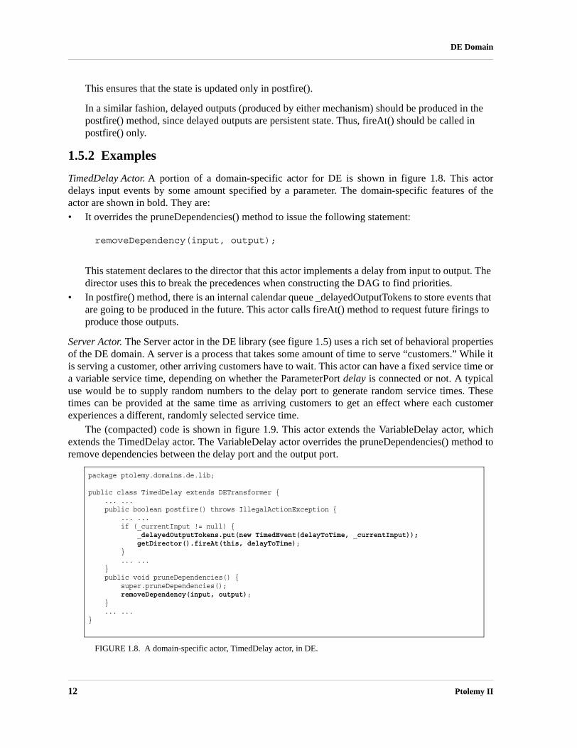
TimedDelay Actor. A portion of a domain-specific actor for DE is shown in figure 1.8. This actordelays input events by some amount specified by a parameter. The domain-specific features of theactor are shown in bold. They are:• It overrides the pruneDependencies() method to issue the following statement:

removeDependency(input, output);

This statement declares to the director that this actor implements a delay from input to output. The director uses this to break the precedences when constructing the DAG to find priorities.

• In postfire() method, there is an internal calendar queue _delayedOutputTokens to store events that are going to be produced in the future. This actor calls fireAt() method to request future firings to produce those outputs.

Server Actor. The Server actor in the DE library (see figure 1.5) uses a rich set of behavioral propertiesof the DE domain. A server is a process that takes some amount of time to serve “customers.” While itis serving a customer, other arriving customers have to wait. This actor can have a fixed service time ora variable service time, depending on whether the ParameterPort delay is connected or not. A typicaluse would be to supply random numbers to the delay port to generate random service times. Thesetimes can be provided at the same time as arriving customers to get an effect where each customerexperiences a different, randomly selected service time.

The (compacted) code is shown in figure 1.9. This actor extends the VariableDelay actor, whichextends the TimedDelay actor. The VariableDelay actor overrides the pruneDependencies() method toremove dependencies between the delay port and the output port.

package ptolemy.domains.de.lib;

public class TimedDelay extends DETransformer { ... ... public boolean postfire() throws IllegalActionException { ... ... if (_currentInput != null) { _delayedOutputTokens.put(new TimedEvent(delayToTime, _currentInput)); getDirector().fireAt(this, delayToTime); } ... ... } public void pruneDependencies() { super.pruneDependencies(); removeDependency(input, output); } ... ...}

FIGURE 1.8. A domain-specific actor, TimedDelay actor, in DE.

12 Ptolemy II

DE Domain

The fire() method first reads and updates the _delay amount. Then it reads the input tokens andstore them into the local event queue that stores the delayed input tokens for future processing in thepostfire() method. In the end, it checks whether there is some output event scheduled to be produced atthe current tag. If there is one, output that event. Otherwise, do nothing.

The postfire() method first removes the output token being produced from the local event queuethat stores delayed output tokens. If the server is free at the current time, then this actor schedules afuture firing to handle the remaining inputs. This is done in the postfire() method rather than the fire()method in keeping with the policy in Ptolemy II that persistent state is not updated in the fire() method.

Note that if an actor does not consume input tokens that are available in the fire() method, it isessential that prefire() returns false. Otherwise, the DE scheduler will keep firing the actor until theinputs are all consumed, which will never happen if the actor is not consuming inputs!

package ptolemy.domains.de.lib;

public class Server extends VariableDelay { public PortParameter delay; public void fire() throws IllegalActionException { delay.update(); _delay = ((DoubleToken) delay.getToken()).doubleValue(); Time currentTime = getDirector().getModelTime(); if (input.hasToken(0)) { _currentInput = input.get(0); _delayedInputTokensList.addLast(_currentInput); } else { _currentInput = null; } _currentOutput = null; if (_delayedOutputTokens.size() > 0) { if (currentTime.compareTo(_nextTimeFree) == 0) { TimedEvent earliestEvent = (TimedEvent) _delayedOutputTokens.get(); Time eventTime = earliestEvent.timeStamp; if (!eventTime.equals(currentTime)) { throw new InternalErrorException("Service time is " + "reached, but output is not available."); } _currentOutput = (Token) earliestEvent.contents; output.send(0, _currentOutput); } } } public void initialize() throws IllegalActionException { super.initialize(); _nextTimeFree = Time.NEGATIVE_INFINITY; _delayedInputTokensList = new LinkedList(); } public boolean postfire() throws IllegalActionException { Time currentTime = getDirector().getModelTime(); if (_currentOutput != null) { _delayedOutputTokens.take(); } if ((_delayedInputTokensList.size() != 0) && _delayedOutputTokens.isEmpty()) { _nextTimeFree = currentTime.add(_delay); _delayedOutputTokens.put(new TimedEvent(_nextTimeFree, _delayedInputTokensList.removeFirst())); getDirector().fireAt(this, _nextTimeFree); } return !_stopRequested; }}

FIGURE 1.9. Code for the Server actor. For more details, see the source code.


DE Domain

1.5.3 Thread Actors1

In some cases, it is useful to describe an actor as a thread that waits for input tokens on its inputports. The thread suspends while waiting for input tokens and is resumed when some or all of its inputports have input tokens. While this description is functionally equivalent to the standard descriptionexplained above, it leverages on the Java multi-threading infrastructure to save the state information.

Consider the code for the ABRecognizer actor shown in figure 1.10. The two code listings imple-ment two actors with equivalent behavior. The left one implements it as a threaded actor, while theright one implements it as a standard actor. We will from now on refer to the left one as the threadeddescription and the right one as the standard description. In both descriptions, the actor has two inputports, inportA and inportB, and one output port, outport. The behavior is as follows.

Produce an output event at outport as soon as events at inportA and inportB occursin that particular order, and repeat this behavior.

Note that the standard description needs a state variable state, unlike the case in the threadeddescription. In general the threaded description encodes the state information in the position of thecode, while the standard description encodes it explicitly using state variables. While it is true that thecontext switching overhead associated with multi-threading application reduces the performance, weargue that the simplicity and clarity of writing actors in the threaded fashion is well worth the cost insome applications.

To write an actor in the threaded fashion, one simply derives from the DEThreadActor class andimplements the run() method. In many cases, the content of the run() method is enclosed in the infinite‘while(true)’ loop since many useful threaded actors do not terminate.

The waitForNewInputs() method is overloaded and has two flavors, one that takes no arguments

1. This section describes techniques that have not been widely used, and are not extensively tested.

public class ABRecognizer extends DEThreadActor {StringToken msg = new StringToken("Seen AB");

// the run method is invoked when the thread// is started.public void run() {

while (true) {waitForNewInputs();if (inportA.hasToken(0)) {

IOPort[] nextInport = {inportB};waitForNewInputs(nextInport);outport.broadcast(msg);

}}

}

public class ABRecognizer extends DEActor {StringToken msg = new StringToken("Seen AB");

// We need an explicit state variable in// this case.int state = 0;

public void fire() {switch (state) {

case 0:if (inportA.hasToken(0)) {

state = 1;break;

}case 1:

if (inportB.hasToken(0)) {state = 0;outport.broadcast(msg);

}}

}}

FIGURE 1.10. Code listings for two style of writing the ABRecognizer actor.

14 Ptolemy II

DE Domain

and another that takes an IOPort array as argument. The first suspends the thread until there is at leastone input token in at least one of the input ports, while the second suspends until there is at least oneinput token in any one of the specified input ports, ignoring all other tokens.

In the current implementation, both versions of waitForNewInputs() clear all input ports before thethread suspends. This guarantees that when the thread resumes, all tokens available are new, in thesense that they were not available before the waitForNewInput() method call.

The implementation also guarantees that between calls to the waitForNewInputs() method, the restof the DE model is suspended. This is equivalent to saying that the section of code between calls to thewaitForNewInput() method is a critical section. One immediate implication is that the result of themethod calls that check the configuration of the model (e.g. hasToken() to check the receiver) will notbe invalidated during execution in the critical section. It also means that this should not be viewed as away to get parallel execution in DE. For that, consider the DDE domain.

It is important to note that the implementation serializes the execution of threads, meaning that atany given time there is only one thread running. When a threaded actor is running (i.e. executing insideits run() method), all other threaded actors and the director are suspended. It will keep running until awaitForNewInputs() statement is reached, where the flow of execution will be transferred back to thedirector. Note that the director thread executes all non-threaded actors. This serialization is neededbecause the DE domain has a notion of global time, which makes parallelism much more difficult toachieve.

The serialization is accomplished by the use of monitor in the DEThreadActor class. Basically, thefire() method of the DEThreadActor class suspends the calling thread (i.e. the director thread) until thethreaded actor suspends itself (by calling waitForNewInputs()). One key point of this implementationis that the threaded actors appear just like an ordinary DE actor to the DE director. The DEThreadActorbase class encapsulates the threaded execution and provides the regular interfaces to the DE director.Therefore the threaded description can be used whenever an ordinary actor can, which is everywhere.

The code shown in figure 1.11 implements the run method of a slightly more elaborate actor withthe following behavior:

Emit an output O as soon as two inputs A and B have occurred. Reset this behavioreach time the input R occurs.

Recent work has extended the DE Director to support parallel execution in the form of actors contain-ing private threads and callbacks. Future work in this area may involve extending the infrastructure tosupport additional concurrency constructs, such as preemption, other forms of parallel execution, etc.It might also be interesting to explore new concurrency semantics similar to the threaded DE, but with-out the ‘forced’ serialization.

1.6 Composing DE with Other Domains

One of the major concepts in Ptolemy II is modeling heterogeneous systems through the use ofhierarchical heterogeneity. Actors on the same level of hierarchy obey the same set of semantics rules.Inside some of these actors may be another domain with a different model of computation. This mech-anism is supported through the use of opaque composite actors. An example is shown in figure 1.12.The outermost domain is DE and it contains seven actors, two of them are opaque and composite. Theopaque composite actors contain subsystems, which in this case are in the DE and CT domains.


DE Domain

1.6.1 DE inside Another Domain

The DE subsystem completes one iteration whenever the opaque composite actor is fired by theouter domain. One of the complications in mixing domains is in the synchronization of time. Denotethe current time of the DE subsystem by tinner and the current time of the outer domain by touter. Aniteration of the DE subsystem is similar to an iteration of a top-level DE model, except that prior to theiteration tokens are transferred from the ports of the opaque composite actors into the ports of the con-tained DE subsystem, and after the end of the iteration, the director requests a refire at the smallesttime stamp in the event queue of the DE subsystem. This presumes that the DE subsystem knows atwhat time stamp the it, or one of its contained actors, will wish to be refired. Future work may removethis limitation, allowing real-time events (such as from I/O) to propagate out of a DE subsystem. Cur-rently the DE domain can handle such asynchronous events only if it is not inside another domain.

public void run() {try {

while (true) {// In initial state..waitForNewInputs();if (R.hasToken(0)) {

// Resetting..continue;

}if (A.hasToken(0)) {

// Seen A..IOPort[] ports = {B,R};waitForNewInputs(ports);if (!R.hasToken(0)) {

// Seen A then B..O.broadcast(new DoubleToken(1.0));IOPort[] ports2 = {R};waitForNewInputs(ports2);

} else {// Resettingcontinue;

}} else if (B.hasToken(0)) {

// Seen B..IOPort[] ports = {A,R};waitForNewInputs(ports);if (!R.hasToken(0)) {// Seen B then A..O.broadcast(new DoubleToken(1.0));IOPort[] ports2 = {R};waitForNewInputs(ports2);

} else {// Resettingcontinue;

}} // while (true)

} catch (IllegalActionException e) {getManager().notifyListenersOfException(e);

}}

FIGURE 1.11. The run() method of the ABRO actor.

16 Ptolemy II

DE Domain

The transfer of tokens from the ports of the opaque composite actor into the ports of the containedDE subsystem actors is done in the transferInputs() method of the DE director. This method isextended from its default implementation in the Director class. The implementation in the DEDirectorclass advances the current time of the DE subsystem to the current time of the outer domain, then callssuper.transferInputs(). It is done in order to correctly associate tokens seen at the input ports of theopaque composite actor, if any, with events at the current time of the outer domain, touter, and put theseevents into the global event queue. This mechanism is, in fact, how the DE subsystem synchronize itscurrent time, tinner, with the current time of the outer domain, touter.(Recall that the DE directoradvances time by looking at the smallest time stamp in the event queue of the DE subsystem). Specifi-cally, before the advancement of the current time of the DE subsystem tinner is less than or equal to thetouter, and after the advancement tinner is equal to the touter.

Requesting a refiring is done in the postfire() method of the (inner) DE director by calling thefireAt() method of the executive (outer) director. Its purpose is to ensure that events in the DE sub-system are processed on time with respect to the current time of the outer domain, touter.

Note that if the DE subsystem is fired due to the outer domain processing a refire request, thenthere may not be any tokens in the input port of the opaque composite actor at the beginning of the DEsubsystem iteration. In that case, no new events with time stamps equal to touter will be put into theglobal event queue. Interestingly, in this case, the time synchronization will still work because tinnerwill be advanced to the smallest time stamp in the global event queue which, in turn, has to equal touterbecause we always request a refire according to that time stamp.

K(z)Sin + 1/s 1/s

ZOH

ProcessDelay

InterruptibleServer

DEPoisson

ContinuousTime

DiscreteEvent

Discrete Event

FIGURE 1.12. An example of heterogeneous and hierarchical composition. The CT subsystem and DE subsystem are inside an outermost DE system. This example is developed by Jie Liu [93].


DE Domain

1.6.2 Another Domain inside DE

Due to its nature, any opaque composite actor inside DE is opaque and therefore, as far as the DEDirector is concerned, behaves exactly like a domain polymorphic actor. Recall that domain polymor-phic actors are treated as functions with zero delay in computation time. To produce events in thefuture, domain polymorphic actors request a refire from the DE director and then produce the eventswhen it is refired.

18 Ptolemy II

Heterogeneous Concurrent Modeling and D

2
CT Domain
Author: Jie LiuHaiyang Zheng

2.1 Introduction

The continuous-time (CT) domain in Ptolemy II aims to help the design and simulation of systemsthat can be modeled using ordinary differential equations (ODEs). ODEs are often used to model ana-log circuits, plant dynamics in control systems, lumped-parameter mechanical systems, lumped-parameter heat flows and many other physical systems.

Let’s start with an example. Consider a second order differential system,

(1)

The equations could be a model for an analog circuit as shown in figure 2.1(a), where z is the voltage

mz·· t( ) bz· t( ) kz t( )+ + u t( )y t( ) c z t( )z 0( )

⋅10 z· 0( ), 0.=

===

+-

u

R1 R2 R3

R4C1 C2 y

+

-

z

+

-

(a) A circuit implementation.

FIGURE 2.1. Possible implementations of the system equations.

(b) A mechanical implementation.

1 2 3I1

Substrate

proof-mass

mz

Fk Fbk b

u

esign 19

CT Domain

of node 3, and

(2)

Or it could be a lumped-parameter spring-mass mechanical model for the system shown in figure2.1(b), where z is the position of the mass, m is the mass, k is the spring constant, b is the dampingparameter, and c = 1.

In general, an ODE-based continuous-time system has the following form:

(3)

(4)

, (5)

where, , , a real number, is continuous time. At any time t, , an n-tuple of real num-bers, is the state of the system; is the m-dimensional input of the system; is the l-dimensional output of the system; is the derivative of with respect to time , i.e.

. (6)

Equations (3), (4), and (5) are called the system dynamics, the output map, and the initial condition ofthe system, respectively.

For example, for the mechanical system above, if we define a vector

, (7)

then system (1) can be written in form of (3)-(5), like

(8)

The solution, x(t), of the set of ODE (3)-(5), is a continuous function of time, also called a wave-form, which satisfies the equation (3) and initial condition (5). The output of the system is then definedas a function of x(t) and u(t), which satisfies (4). The precise solution of a set of ODEs is usuallyimpossible to be found using digital computers. Numerical solutions are approximations of the precisesolution. A numerical solution of ODEs are usually done by integrating the right-hand side of (3) on adiscrete set of time points. Using digital computers to simulate continuous-time systems has been stud-ied for more than three decades. One of the most well-known tools is Spice [112]. The CT domain dif-fers from Spice-like continuous-time simulators in two ways — the system specification is somewhatdifferent, and it is designed to interact with other models of computation.

m R1 R2 C1 C2k

⋅ ⋅⋅R1 C1 R2 C2

b⋅+⋅

1c R4 R3 R4+( )⁄ .

====

x· f x u t, ,( )=

y g x u t, ,( )=

x t0( ) x0=

t ℜ∈ t t0≥ x ℜn∈u ℜm∈ y ℜl∈

x· ℜn∈ x t

x·dxdt------=

x t( ) z t( )z· t( )

=

x· t( ) 1m---- 0 1

k– b–x t( ) 0

1 m⁄u t( )

y t( )

+

c 0 x t( )

x 0( ) 10

0.

=

=

=

20 Ptolemy II

CT Domain

2.1.1 System Specification

There are usually two ways to specify a continuous-time system, the conservation-law model andthe signal-flow model [63]. The conservation-law models, like the nodal analysis in circuit simulation[60] and bond graphs [128] in mechanical models, define systems by their physical components, whichspecify relations of cross and through variables, and conservation laws are used to compile the compo-nent relations into global system equations. For example, in circuit simulation, the cross variables arevoltages, the through variables are currents, and the conservation laws are Kirchhoff’s laws. Thismodel directly reflects the physical components of a system, thus is easy to construct from a potentialimplementation. The actual mathematical representation of the system is hidden. In signal-flow mod-els, entities in a system are maps that define the mathematical relation between their input and outputsignals. Entities communicate by passing signals. This kind of models directly reflects the mathemati-cal relations among signals, and is more convenient for specifying systems that do not have an explicitphysical implementation yet.

In the CT domain of Ptolemy II, the signal-flow model is chosen as the interaction semantics. Theconservation-law semantics may be used within an entity to define its I/O relation. There are fourmajor reasons for this decision:

1. The signal-flow model is more abstract. Ptolemy II focuses on system-level design and behavior simulation. It is usually the case that, at this stage of a design, users are working with abstract mathematical models of a system, and the implementation details are unknown or not cared about.

2. The signal flow model is more flexible and extensible, in the sense that it is easy to embed compo-nents that are designed using other models. For example, a discrete controller can be modeled as a component that internally follows a discrete event model of computation but exposes a continu-ous-time interface.

3. The signal flow model is consistent with other models of computation in Ptolemy II. Most models of computation in Ptolemy use message-passing as the interaction semantics. Choosing the signal-flow model for CT makes it consistent with other domains, so the interaction of heterogeneous systems is easy to study and implement. This also allows domain polymorphic actors to be used in the CT domain.

4. The signal flow model is compatible with the conservation law model. For physical systems that are based on conservation laws, it is usually possible to wrap them into an entity in the signal flow model. The inputs of the entity are the excitations, like the current on ideal current sources, and the outputs are the variables that the rest of the system may be interested in.The signal flow block diagram of the system (3) - (5) is shown in figure 2.2. The system dynamics

(3) is built using integrators with feedback. In this figure, u, , x, and y, are continuous signals flowingfrom one block to the next. Notice that this diagram is only conceptual, most models may involve mul-

FIGURE 2.2. A conceptual block diagram for continuous time systems.

g( )f( )u yxx

.

x·


CT Domain

tiple integrators1. Time is shared by all components, so it is not considered as an input. At any fixedtime t, if the “snapshot” values x(t) and u(t) are given, then and y(t) can be found by evaluating fand g, which can be achieved by firing the respective blocks. The “snapshot” of all the signals at iscalled the behavior of the system at time .

The signal-flow model for the example system (1) is shown in figure 2.3. For comparison purpose,the conservation-law model (modified nodal analysis) of the system shown in figure 2.1(a) is shown in(9).

(9)

By doing some math, we can see that (9) and (8) are in fact equivalent. Equation (9) can be easilyassembled from the circuit, but it is more complicated than (8). Notice that in (9) is the derivativeoperator, which is replaced by an integration algorithm at each time step, and the system equationsreduce to a set of algebraic equations. Spice software is known to have a very good simulation enginefor models in form of (9).

2.1.2 Time

One distinct characterization of the CT model is the continuity of time. This implies that a contin-uous-time system have a behavior at any time instance. The simulation engine of the CT model shouldbe able to compute the behavior of the system at any time point, although it may march discretely intime. In order to achieve an accurate simulation, time should be carefully discretized. The discretiza-tion of time, which appears as integration step sizes, may be determined by time points of interest (e.g.

1. Ptolemy II does not support vectorization in the CT domain yet.

x· t( )t

t

u + C

-b/m

-k/m

y1/m

U G1 A S1 S2 G4 Y

G2

G3

FIGURE 2.3. The block diagram for the example system.

1R1------- 1

R1-------– 0 0 1–

1R1-------–

1R1------- 1

R2------- C1

ddt-----+ +

1R2-------– 0 0

01

R2-------–

1R2------- 1

R3------- C2

ddt-----+ +

1R3-------– 0

0 01

R3-------–

1R3------- 1

R4-------+ 0

1 0 0 0 0

v1

v2

v3

y

I1

0

0

0

0

u

=

d/dt

22 Ptolemy II

CT Domain

discontinuities), by the numerical error of integration, and by the convergence in solving algebraicequations.

Time is also global, which means that all components in the system share the same notion of time.

2.2 Solving ODEs numerically

We outline some basic terminologies on numerical ODE solving techniques that are used in thischapter. This is not a summary of numerical ODE solving theory. For a detailed treatment for ODEsand their numerical solutions, please refer to books on numerical solutions for ODEs, e.g. [45].

Not all ODEs have a solution, and some ODEs have more than one solution. In such situations, wesay that the solution is not well defined. This is usually a result of errors in the system modeling. Werestrict our discussion to systems that have unique solutions. Theorem 1 in Appendix A states the con-ditions for the existence and uniqueness of solutions of ODEs. Roughly speaking, we denote by D a setin which contains at most a finite number of points per unit interval, and let u be piecewise-contin-uous on . Then, for any fixed u(t), if f is also piecewise-continuous on , and f satisfies theLipschitz condition (see e.g. [45]), then the ODE (3) with the initial condition (5) has a unique solu-tion. The solution is called the state trajectory of the system. The key of simulating a continuous-timesystem numerically is to find an accurate numerical approximation of the state trajectory.

2.2.1 Basic Notations

Usually, only the solution on a finite time interval is needed. A simulation of the system isperformed on discrete time points in this interval. We denote by

, (10)

where

, (11)

the set of the discrete time points of interest. To explicitly illustrate the discretization of time and thedifference between the precise solution and the numerical solution, we use the following notation inthe rest of the chapter:• : the n-th time point, to explicitly show the discretization of time. However, we write t, if the

index n is not important.• : the precise (continuous) state trajectory from time to ;• : the precise solution of (3) at time ;

• : the numerical solution of (3) at time ;

• : step size of numerical integration. We also write if the index n in the sequence

is not important. For accuracy reason, may not be uniform.

• : the 2-normed difference between the precise solution and the numerical solution at

step n is called the (global) error at step n; the difference, when we assume are precise,

is called the local error at step n. Local errors are usually easy to estimate and the estimation can be used for controlling the accuracy of numerical solutions.

ℜℜ D– ℜ D–

t0 tf[ , ]

Tc t0 t1 t2 …tn …tf,, , ,{ } Tc, t0 tf,[ ]⊂=

t0 t1 t2 … tn … tf< < < < < <

tn

x ti tj,[ ] ti tj

x tn( ) tn

xtntn

hn tn tn 1––= h

h

x tn( ) xtn–

xt0…xtn 1–


CT Domain

A general way of numerically simulating a continuous-time system is to compute the state and theoutput of the system in an increasing order of . Such algorithms are called the time-marching algo-rithms, and, in this chapter, we only consider these algorithms. There are variety of time marchingalgorithms that differ on how is computed given . The choice of algorithms is applica-tion dependent, and usually reflects the speed, accuracy, and numerical stability trade-offs.

2.2.2 Fixed-Point Behavior

Numerical ODE solving algorithms approximate the derivative operator in (3) using the historyand the current knowledge on the state trajectory. That is, at time , the derivative of x is approxi-mated by a function of , i.e.

. (12)

Plugging (3) in this, we get

(13)

Depending on whether explicitly appears in (13), the algorithms are called explicit integrationalgorithms or implicit integration algorithms. That is, we end up solving a set of algebraic equations inone of the two forms:

(14)

or

, (15)

where are derived from the time , the input , the function f, and the history of xand . Solving (14) or (15) at a particular time is called an iteration of the CT simulation at .

Equation (14) can be solved simply by a function evaluation and an assignment. But the solutionof (15) is the fixed point of FI, which may not exist, may not be unique, or may not be able to be found.The contraction mapping theorem [21] shows the existence and uniqueness of the fixed-point solution,and provides one way to find it. Given the map FI that is a local contraction map (generally true forsmall enough step sizes) and let an initial guess be in the contraction radius, then a unique fixedpoint exists and can be found by iteratively computing:

(16)

Solving both (14) and (15) should be thought of as finding the fixed-point behavior of the systemat a particular time. This means both functions should be smooth w.r.t. time, during oneiteration of the simulation. This further implies that the topology of the system, all the parameters, andall the internal states that the firing functions depend on should be kept unchanged. We require thatdomain polymorphic actors to update internal states only in the postfire() method exactly for thisreason.

2.2.3 ODE Solvers Implemented

The following solvers has been implemented in the CT domain.

tn

xtnxt0

…xtn 1–

tnxt0

… xtn 1–xtn

, , ,

x· tnp xt0

… xtn 1–xtn

, , ,( )=

p xt0…xtn 1–

xtn,( ) f xtn

u tn( ) tn,,( )=

xtn

xtnFE xt0

… x, ,tn 1–

( )=

FI xt0… x, ,

tn( ) 0=

FE and FI tn u tn( )x· tn tn

σ0

σ1 FE σ0( ), σ2 FE σ1( ), σ3 FE σ2( ), …= = =

FE and FI

24 Ptolemy II

CT Domain

1. Forward Euler solver:

(17)

2. 2(3)-order Explicit Runge-Kutta solver

(18)

with error control:

(19)

if , , otherwise, fail. If this step is successful, the next integration step size is predicted by:

(20)

3. 4(5)-order Explicit Runge-Kutta solver1

(21)

1. This algorithm is based on "A Variable Order Runge-Kutta Method for Initial Value Problems with Rapidly Varying Right-Hand Sides" by J. R. Cash and A. H. Karp, ACM Transactions on Mathematical Software, 16(3), 201-222 (1990).

xtn 1+xtn

hn 1+ x· tn

⋅+

xtnhn 1+ f xtn

utntn, ,( )⋅+

=

=

K0 hn 1+ f xtnutn

tn, ,( )

K1

⋅

hn 1+ f xtnK0 2⁄ utn hn 1+ 2⁄+ tn hn 1+ 2⁄+, ,+( )

K2

⋅

hn 1+ f xtn3K1 4⁄+ utn 3hn 1+ 4⁄+ tn 3hn 1+ 4⁄+, ,( )⋅

x̃tn 1+xtn

29---K0

13---K1

49---K2+ + +

=

=

=

=

K3 hn 1+ f x̃tn 1+utn 1+

tn 1+, ,( )

LTE

⋅

572------K0–

112------K1

19---K2

18---K3–+ +

=

=

LTE ErrorTolerance< xtn 1+x̃tn 1+

=

hn 2+ hn 1+ max 0.5 0.8 ErrorTolerance( ) LTE⁄3⋅,( )⋅=

K0 hn 1+ f xtnutn

tn, ,( )

K1

⋅

hn 1+ f xtnK0 5⁄ utn hn 1+ 5⁄+ tn hn 1+ 5⁄+, ,+( )

K2

⋅

hn 1+ f xtn3K0 40⁄ 9K1 40⁄+ + utn 3hn 1+ 10⁄+ tn 3hn 1+ 10⁄+, ,( )⋅

K3 hn 1+ f xtn3K0 10⁄ 9K1 10⁄– 6K2 5⁄+ + utn 3hn 1+ 5⁄+ tn 3hn 1+ 5⁄+, ,( )⋅

K4 hn 1+ f xtn11K0 54⁄– 5K1 2⁄ 70K2 27⁄– 35K3 27⁄+ + utn hn 1++ tn hn 1++, ,( )

K5 hn 1+ f xtn1631K0 55296⁄ 175K1 512⁄ 575K2 13824⁄ 44275K3 110592⁄

253K4 4096⁄

+ + + +

+ utn 7hn 1+ 8⁄+ tn 7hn 1+ 8⁄+, ,

(

)

⋅=

⋅

x̃tn 1+xtn

37378---------K0

250621---------K1

125594---------K2

5121771------------K5+ + + +

=

=

=

=

=

=


CT Domain

with error control:

(22)

if , , otherwise, fail. If this step is successful, the next integration step size is predicted by:

(23)

4. Backward Euler solver:

(24)

5. Trapezoidal Rule solver:

. (25)

Among these solvers, 1), 2) and 3) are explicit; 4) and 5) are implicit. Also, 1) and 4) do not per-form step size control, so are called fixed-step-size solvers; 2), 3), and 5) change step sizes accordingto error estimation, so are called variable-step-size solvers. Variable-step-size solvers adapt the stepsizes according to changes of the system flow, thus are “smarter” than fixed-step-size solvers.

2.2.4 Discontinuity

The existence and uniqueness of the solution of an ODE (Theorem 1 in Appendix A) allows theright-hand side of (3) to be discontinuous at a discrete set D1, and the elements in this discrete set arecalled the breakpoints (also called the discontinuous points in some literature). These breakpoints maybe caused by the discontinuity of input signal u, or by the intrinsic flow of f. At these points, the solu-tions are defined based on a discrete-event semantics and achieved by performing discrete phase ofexecutions. Discrete phase of executions solve the final values at breakpoints, which are the solutionsdefined on the right limits. The left limits of the solutions, which are called initial values at break-points, are solved with the normal continuous-time equations based on the ODE.

One impact of breakpoints on ODE solvers is that history solutions are useless when approximat-ing the derivative of x after the breakpoints. The solver should resolve the new initial conditions andstart the solving process as if it is at a starting point. So, the discretization of time should step exactlyon breakpoints for the left limit, and start at the breakpoint again after finding the right limit.

A breakpoint may be known beforehand, in which case it is called a predictable breakpoint. For

1. A discrete set is an ordered set for which there exists an order embedding to the natural numbers.

K6 hn 1+ f x̃tn 1+utn 1+

tn 1+, ,( )

LTE

⋅

37378--------- 2825

27648---------------–

K0250621--------- 18575

48384---------------–

K2125594--------- 13525

55296---------------–

K3277

14336---------------K4–

5121771------------ 1

4---–

K5

+ +

+

=

=

LTE ErrorTolerance< xtn 1+x̃tn 1+

=

hn 2+ hn 1+ ErrorTolerance( ) LTE⁄5⋅=

xtn 1+xtn

hn 1+ x· tn 1+

⋅+

xtnhn 1+ f xtn 1+

utn 1+tn 1+, ,( )⋅+

=

=

xtn 1+xtn

hn 1+

2------------ x· tn

x· tn 1++( )

+

xtn

hn 1+

2------------ x· tn

f xtn 1+utn 1+

tn 1+, ,( )+( )+

=

=

26 Ptolemy II

CT Domain

example, a square wave source actor knows its next flip time. This information can be used to controlthe discretization of time. A breakpoint can also be unpredictable, which means it is unknown until thetime it occurs is passed. For example, an actor that varies its functionality when the input signalcrosses a threshold can only report a “missed” breakpoint after an integration step is finished. How tohandle breakpoints correctly is a big challenge for integrating continuous-time models with discretemodels like DE and FSM.

2.2.5 Breakpoint ODE Solvers

Breakpoints in the CT domain are handled by adjusting integration steps. We use a table to handlepredictable breakpoints, and use the step size control mechanism to handle unpredictable breakpoints.The breakpoint handling are transparent to users, and the implementation details (provided in section2.8.4) are only needed when developing new directors, solvers, or event generators.

Since the history information is useless at breakpoints, a special ODE solver is designed to restartthe numerical integration process. In particular, we have implemented the DerivativeResolver, whichcalculates the derivative of the current state, i.e. . This is simply done by evaluation theright-hand side of (3). At breakpoints, this solver is used for the first step to generate history informa-tion for explicit methods or one step methods. Notice that this solver does not advance time and it canonly be used at breakpoints.

2.3 Signal Types

The CT domain of Ptolemy II supports continuous time mixed-signal modeling. As a consequence,there could be two types of signals in a CT model: continuous signals and discrete events. Note that forboth types of signals, time is continuous. These two types of signals directly affect the behavior of areceiver that contains them. A continuous CTReceiver contains a sample of a continuous signal at thecurrent time. Reading a token from that receiver will not consume the token. A discrete CTReceivermay or may not contain a discrete event. Reading from a discrete CTReceiver with an event will con-sume the event, so that events are processed exactly once1. Reading from an empty discrete CTRe-ceiver is not allowed.

Note that some actors can be used to compute on both continuous and discrete signals. For exam-ple, an adder can add two continuous signals, as well as two sets of discrete events. Whether a particu-lar link among actors is continuous or discrete is resolved by a signal type system. The signal typesystem understands signal types on specific actors (indicated by the interfaces they implement or theparameters specified on their ports), and try to resolve signal types on the ports of domain polymorphicactors.

The signal type system in the CT domain works on a simple lattice of signal types, shown in Fig-ure 2.4. A type lower in the lattice is more specific than a type higher in the lattice. A CT model iswell-defined and executable, if and only if all ports are resolved to either CONTINUOUS or DIS-CRETE. Some actors have their signal types fixed. For example, an Integrator has a CONTINU-OUS input and a CONTINUOUS output; a PeriodicSampler has a CONTINUOUS input and aDISCRETE output; a TriggeredSampler has one CONTINUOUS input (the input), one DIS-CRETE input (the trigger), and a DISCRETE output; and a ZeroOrderHold has a DISCRETE inputand a CONTINUOUS output. For domain polymorphic actors that implement the SequenceActor

1. This distinction of receivers is also called state and event semantics in some literatures [70].

dx( ) dt( )⁄


CT Domain

interface, i.e. they operate solely on sequences of tokens, their inputs and outputs are treated as DIS-CRETE. For other domain polymorphic actors that can operate on both continuous and discrete sig-nals, the signal type on their ports are initially UNRESOLVED. The signal type system will resolveand check signal types of ports according to the following two rules:• If a port p is connected to another port q with a more specific type, then the type of p is resolved to

that of the port q. If p is CONTINUOUS but q is DISCRETE, then both of them are resolved to NOT-A-TYPE.

• Unless otherwise specified, the types of the input ports and output ports of an actor are the same.At the end of the signal-type resolution, if any port is of type UNRESOLVED or NOT-A-TYPE,

then the topology of the system is illegal, and the execution is denied.The signal type of a port can also be forced by adding an parameter “signalType” to the port. The

signal type system will recognize this parameter and resolve other types accordingly. To add thisparameter, right click on the port, select Configure, then add a parameter with the name signalType andthe value of a string of either “CONTINUOUS” or “DISCRETE”, noting the quotation marks.

Signal types may be more trickier at the boundaries of opaque composite actors than within a CTmodel. Because of the information hiding, it may not be obvious which port of another level of hierar-chy is continuous and which port is discrete. In the CT domain, we follow these rules to resolve signaltypes for composite ports:• A TypedCompositeActor within a CT model is always treated as entirely discrete. Within a CT

model, for any opaque composite actor that may contain continuous dynamics at a deeper level, use the CTCompositeActor (listed in the actor library as “continuous time composite actor” in domain specific actors) or the modal model composite actor.

• For a CTCompositeActor or a modal model within a CT model, all its ports are treated as contin-uous by default. To allow a discrete event going through the composite actor boundary, manually set the signal type of that port by adding the signalType parameter.

• For a TypedCompositeActor containing a CT model, all the ports of the TypedCompositeAc-tor are treated as discrete, and the CT director to use is the CTMixedSignalDirector (listed as CTDirector in the vergil director library).

• For a CTCompositeActor or a modal model containing a CT model, all the signal types of the ports of the container are treated as continuous, and can be set by adding the signalType parameter. The CTDirector to use in this situation is the CTEmbeddedDirector.

UNRESOLVED

CONTINUOUS DISCRETE

NOT-A-TYPE

FIGURE 2.4. A signal type lattice.

28 Ptolemy II

CT Domain

2.4 CT Actors

A CT system can be built up using actors in the ptolemy.domains.ct.lib package and domain poly-morphic actors that have continuous behaviors (i.e. all actors that do not implement the SequenceActorinterface). The key actor in CT is the integrator. It serves the unique role of wiring up ODEs. Otheractors in a CT system are usually stateless. A general understanding is that, in a pure continuous-timemodel, all the information — the state of the system— is stored in the integrators.

2.4.1 CT Actor Interfaces

In order to schedule the execution of actors in a CT model and to support the interaction betweenCT and other domains (which are usually discrete), we provide the following interfaces.• CTDynamicActor. Dynamic actors are actors that contains continuous dynamics in their I/O path.

An integrator is a dynamic actor, and so are all actors that have integration relations from their inputs to their outputs.

• CTEventGenerator. Event generators are actors that convert continuous time input signals to dis-crete output signals.

• CTStatefulActor. Stateful actors are actors that have internal states. The reason to classify this kind of actor is to support rollback, which may happen when a CT model is embedded in a discrete event model.

• CTStepSizeControlActor. Step size control actors influence the integration step size by telling the director whether the current step is accurate. The accuracy is in the sense of both tolerable numerical errors and absence of unpredictable breakpoints. It may also provide information about refining a step size for an inaccurate step and suggesting the next step size for an accurate step.

• CTWaveformGenerator. Waveform generators are actors that convert discrete input signals to continuous-time output signals. Strictly speaking, event generators and waveform generators do not belong to any domain, but the

CT domain is design to handle them intrinsically. When building systems, CT parts always providediscrete interface to other domains.

A loop containing only dynamic actors or a loop containing only non-dynamic actors are notallowed in a CT model. They introduce problems about the order that actors are executed. A loop onlycontaining dynamic actors can be easily broken by a Scale actor with scale 1. A loop of non-dynamicactors builds an algebraic equation. The CT domain does not support modeling algebraic equations,yet.

2.4.2 Actor Library

ContinuousClock. This clock actor generates a periodic continuous-time signal with regularly spacedintervals. The time interval is specified by the period and offset parameters, where the offset parametercontains an array of strictly increasing values that do not exceed the period value. The values of thesignal are specified by the values parameter. The values parameter also contains an array and thelength of this array should be the same as the array length of the offset parameter. This clock actor isdifferent from the normal clock actor (called DiscreteClock) in the actor.lib directory in two ways.First, this actor has a value at any time point. Second, at each offset, this actor produces two values,where the first one is the left limit and second value is the right limit.


CT Domain

ContinuousTransferFunction. A transfer function in the continuous time domain. This actor imple-ments a transfer function where the single input (u) and single output (y) can be expressed in (Laplace)transfer function form as the following equation:

(26)

where m and n are the number of numerator and denominator coefficients, respectively. This actorshas two parameters − numerator and denominator − containing the coefficients of the numerator anddenominator in descending powers of s. The parameters are double arrays. The order of the denomina-tor (n) must be greater than or equal to the order of the numerator (m).

CTPeriodicalSampler. This event generator periodically samples the input signal and generates eventswith the value of the input signal at these time points. The values are always the initial values of theinput signal. The sampling rate is given by the samplePeriod parameter, which has default value 0.1.The sampling time points, which are known beforehand, are examples of predictable breakpoints.

CTRateLimiter. This actor limits the first derivative of the input signal so that the output signal doesnot change faster than the specified limit.

CTTriggeredSampler. This actor samples the continuous input signal when there is a discrete eventpresent at the trigger input. Note that this sampler can generate values other than initial values of theinput signal.

DifferentialSystem. The differential system model implements a system whose behavior is definedby:

(27)

where x is the state vector, u is the input vector, and y is the output vector, t is the time. Users mustgive the name of the variables by filling in the parameter and add ports with proper names. The actor,upon creation, has no inputs and no outputs. After creating proper ports, their names can be used in theexpressions of state equations and output equations. The name of the state variables are manuallyadded by filling in the stateVariableNames parameter.

The state equations and output maps must be manually created by users as parameters. If there aren state variables then users need to create n additional parameters, one for each state equation.And the parameters must be named as x1_dot, ..., xn_dot, respectively. Similarly, if the output portshave names , then users must create additional r parameters for output maps. These parametersshould be named y1, ..., yr, respectively.

EventSource. This actor outputs a set of events at a discrete set of time points. It can be used to gener-ate impulses in CT models.

FirstOrderHold. This actor converts discrete events at the input to a continuous-time signal at the out-put by projecting the value with the derivative.

Y s( )U s( )-----------

b1sm 1–

b2sm 2– … bm+ + +

a1sn 1–

a2sn 2– … an+ + +

-------------------------------------------------------------------=

x· f x u t, ,( )y g x u t, ,( )x t0( ) x0

==

=

x1…xn

y1…yr

30 Ptolemy II

CT Domain

Integrator: The integrator for continuous-time simulation. An integrator has one input port and oneoutput port. Conceptually, the input is the derivative of the output, and an ordinary differential equa-tion is modeled as an integrator with feedback.

An integrator is a dynamic, step-size-control, and stateful actor. To help resolve new states from previous states, a set of variables are used:

• state and its derivative: These are the new state and its derivative at a time point, which have been confirmed by all the step size control actors.

• tentative state and tentative derivative: These are the state and derivative which have not been con-firmed. It is a starting point for other actors to estimate the accuracy of this integration step.

• history: The previous states and derivatives. An integrator remembers the history states and their derivatives for the past several steps. The history is used by multistep methods.

An integrator has one parameter: initialState. At the initialization stage of the simulation, the state of the integrator is set to the initial state. Changes of initialState will be ignored after the simula-tion starts, unless the initialize() method of the integrator is called again. The default value of this parameter is 0.0. An integrator can possibly have several auxiliary variables. These auxiliary variables are used by ODE solvers to store intermediate states for individual integrators.

The CTBaseIntegrator class, which is the super class of Integrator overrides the pruneDependen-cies() method of the AtomicActor class to issue the following statement:

removeDependency(input, output);

This statement declares that the output from an integrator from a firing does not depend on its input. The CT scheduler does not use this information to construct an execution schedule. How-ever, when a CT model works as a subsystem in a DE model, this dependency information is used to help the DE director to construct a DE schedule and assign priorities (execution orders).

LevelCorssingDetector. This actor converts a continuous-time signal to discrete events when the con-tinuous-time signal crosses a level threshold. It has a parameter, errorTolerance, which controls howaccurately the level crossing is determined. The direction parameter can constrain the actor to detectrising crossing only, or falling crossing only, or both. It has three possible values, "rising", "falling",and "both", where "both" is the default. This actor controls the step size such that level crossings neveroccur during an integration. So, this actor is only used in the continuous-time domain. .

LinearStateSpace. The State-Space model implements a system whose behavior is defined by:

(28)

where x is the state vector, u is the input vector, and y is the output vector. The matrix coefficientsmust have the following characteristics:• A must be an n-by-n matrix, where n is the number of states.• B must be an n-by-m matrix, where m is the number of inputs.• C must be an r-by-n matrix, where r is the number of outputs.• D must be an r-by-m matrix.

x· Ax Buy

+Cx Du

x t0( )+x0

==

=


CT Domain

The actor accepts m inputs and generates r outputs through a multiple input port and a multipleoutput port. The widths of the ports must match the number of rows and columns in correspondingmatrices, otherwise, an exception will be thrown.

ThresholdMonitor. This actor controls the integration steps so that the given threshold (on the input) isnot crossed in one step. This actor has one input port and one output port. It has two parameters thresh-oldWidth and thresholdCenter, which have default value 1e-2 and 0, respectively. If the input is withinthe range defined by the threshold center and threshold width, then a true token is emitted from the out-put.

TriggeredContinuousClock. This actor is an extension of the ContinuousClock with a start and stopinput ports. It can only be used in CT models. A token at the start input port will start the clock. Atoken at the stop input port will stop the clock, if it is running. If both start and stop ports receivetokens simultaneously, then the clock will be stopped.

ZeroCrossingDetector. This is an extension of the LevelCrossingDetector actor with the threshold as0.

ZeroOrderHold. This is a waveform generator that converts discrete events into continuous signals.This actor acts as a zero-order hold. It consumes the token when the consumeCurrentEvent() iscalled. This value will be held and emitted every time it is fired, until the next time consumeCur-rentEvent() is called. This actor has one single input port, one single output port, and no parame-ters.

2.4.3 Domain Polymorphic Actors

Not all domain polymorphic actors can be used in the CT domain. Whether an actor can be useddepends on how the internal states of the actor evolve when executing. • Stateless actors: All stateless actors can be used in CT. In fact, most CT systems are built by inte-

grators and stateless actors.• Timed actors: Timed actors change their states according to the notion of time in the model. All

actors that implement the TimedActor interface can be used in CT, as long as they do not also implement SequenceActor. Timed actors that can be used in CT include plotters that are designed to plot timed signals.

• Sequence actors: Sequence actors change their states according to the number of input tokens received by the actor and the number of times that the actor is postfired. Since CT is a time driven model, rather than a data driven model, the number of received tokens and the number of postfires do not have a significant semantic meaning. So, none of the sequence actors can be used in the CT domain. For example, the Ramp actor in Ptolemy II changes its state −− the next token to emit −− corresponding to the number of times that the actor is postfired. In CT, the number of times that the actor is postfired depends on the discretization of time, which further depend on the choice of ODE solvers and setting of parameters. As a result, the slope of the ramp may not be a constant, and this may lead to very counterintuitive models. The same functionality is replaced by a Current-Time actor and a Scale actor. If sequence behaviors are indeed required, event generators and waveform generators may be helpful to convert continuous and discrete signals.

32 Ptolemy II

CT Domain

2.5 CT Directors

There are two CT directors −− CTMixedSignalDirector and CTEmbeddedDirector. A CTMixed-SignalDirector can be used both at the top-level or inside a composite actor, and a CTEmbeddedDirec-tor can only be contained in a CTCompositeActor. In terms of mixing models of computation, bothdirectors can execute composite actors that implement other models of computation, as long as thecomposite actors are properly connected (see section 2.6). Both CTMixedSignalDirector and CTEm-beddedDirector can be contained by other domains. The outside domain of a composite actor withCTMixedSignalDirector can be any discrete domain, such as DE, DT, etc. The outside domain of acomposite actor with CTEmbeddedDirector must also be CT or FSM, if the outside domain of theFSM model is CT. (See also the HSDirector in the FSM domain.)

2.5.1 ODE Solvers

There are six ODE solvers implemented in the ptolemy.domains.ct.kernel.solver package. Thesesolvers are ForwardEulerSolver, BackwardEulerSolver, ExplicitRK23Solver, ExplicitRK45Solver,TrapezoidalRuleSolver, and DerivativeResolver. The DerivativeResolver is specific for handlingbreakpoints. They implement the ODE solving algorithms in section 2.2.3 and section 2.2.5, respec-tively.

2.5.2 CT Director Parameters

The CTDirector base class maintains a set of parameters which controls the execution. Theseparameters, shared by all CT directors, are listed in Table 12 on page 33. Individual directors may havetheir own (additional) parameters, which will be discussed in the appropriate sections.

Table 12: CTDirector Parameters

Name Description TypeDefaultValue

errorTolerance The upper bound of local errors. Actors that perform integration error control (usually integrators in variable step size ODE solving methods) will compare the estimated local error to this value. If the local error estimation is greater than this value, then the integra-tion step is considered inaccurate, and should be restarted with a smaller step sizes.

double 1e-4

initStepSize This is the step size that users specify as the desired step size. For fixed step size solvers, this step size will be used in all non-breakpoint steps. For variable step size solvers, this is only a suggestion.

double 0.1

maxIterations This is used to avoid the infinite loops in (implicit) fixed-point iterations. If the number of fixed-point iterations exceeds this value, but the fixed point is still not found, then the fixed-point procedure is considered failed. The step size will be reduced by half and the integration step will be restarted.

int 20

maxStepSize The maximum step size used in a simulation. This is the upper bound for adjusting step sizes in variable step-size methods. This value can be used to avoid sparse time points when the system dynamic is simple.

double 1.0

minStepSize The minimum step size used in a simulation. This is the lower bound for adjusting step sizes. If this step size is used and the errors are still not tolerable, the simulation aborts. This step size is also used for the first step after breakpoints.

double 1e-5


CT Domain

2.5.3 CTMultiSolverDirector

A CTMultiSolverDirector has two ODE solvers — one for ordinary use and one specifically forbreakpoints. Thus, besides the parameters in the CTDirector base class, this class adds two moreparameters as shown in Table 13 on page 34.

A CTMultiSolverDirector can direct a model that has composite actors implementing other modelsof computation. One simulation iteration is done in two phases: the continuous phase and the discretephase. Let the current iteration be n. In the continuous phase, the differential equations are integratedfrom time to . After that, in the discrete phase, all (discrete) events which happen at are pro-cessed. The step size control mechanism will assure that no events will happen between and .

2.5.4 CTMixedSignalDirector

This director is designed to be the director when a CT subsystem is contained in an event-basedsystem, like DE or DT. As proved in [97], when a CT subsystem is contained in the DE domain, theCT subsystem should run ahead of the global time, and be ready for rollback. This director implementsthis optimistic execution.

Since the outside domain is event-based, each time the embedded CT subsystem is fired, the inputdata are events. In order to convert the events to continuous signals, breakpoints have to be introduced.So this director extends CTMultiSolverDirector, which always has two ODE solvers. There is one

startTime The start time of the simulation. This is only applicable when CT is the top level domain. Otherwise, the CT director follows the time of its executive director.

double 0.0

stopTime The stop time of the simulation. This is only applicable when CT is the top level domain. Otherwise, the CT director follows the time of its executive director.

double Double.MAX_VALUE

synchronizeTo-RealTime

Indicate whether the execution of the model is synchronized to real time at best effort. boolean false

timeResolution This controls the comparison of time. Since time in the CT domain is a double precision real number, it is sometimes impossible to reach or step at a specific time point. If two time points are within this resolution, then they are considered identical.

double 1e-10

valueResolution This is used in (implicit) fixed-point iterations. If in two successive iterations the differ-ence of the states is within this resolution, then the integration step is called converged, and the fixed point is considered reached.

double 1e-6

Table 13: Additional Parameter for CTMultiSolverDirector

Name Description Type Default Value

ODESolver The fully qualified class name for the ODE solver class.

string “ptolemy.domains.ct.kernel.solver.ForwardEulerSolver”

breakpointODESolver The fully qualified class name for the breakpoint ODE solver class.

string “ptolemy.domains.ct.kernel.solver.DerivativeResolver”

Table 12: CTDirector Parameters

Name Description TypeDefaultValue

tn 1– tn tntn 1– tn

34 Ptolemy II

CT Domain

more parameter used by this director — the runAheadLength, as shown in Table 14 on page 35.

When the CT subsystem is fired, the CTMixedSignalDirector will get the current time and thenext iteration time from the outer domain, and take the min( , ) as the fire end time, where is the value of the parameter maxRunAheadLength. The execution lasts as long as the fire end time isnot reached or an output event is not detected.

This director supports rollback; that is when the state of the continuous subsystem is confirmed (byknowing that no events with a time earlier than the CT current time will be present), the state of thesystem is marked. If an optimistic execution is known to be wrong, the state of the CT subsystem willroll back to the latest marked state.

This director can also be used at the top level of a model, which works just as a CTMultipleSolver-Director.

2.5.5 CTEmbeddedDirector

This director is used when a CT subsystem is embedded in another continuous time system, eitherdirectly or through a hierarchy of finite state machines, like in the hybrid system scenario [99]. Thisdirector can pass step size control information up to its executive director. To achieve this, the directormust be contained in a CTCompositeActor, which implements the CTStepSizeControlActor interfaceand can pass the step size control information from the inner domain to the outer domain.

This director extends CTMultiSolverDirector, with no additional parameters. A major differencebetween this director and the CTMixedSignalDirector is that this director does not support rollback. Infact, when a CT subsystem is embedded in a continuous-time environment, rollback is not necessary.

2.6 Interacting with Other Domains

The CT domain can interact with other domains in Ptolemy II. In particular, we consider interac-tion among the CT domain, the discrete event (DE) domain and the finite state machine (FSM)domain. Following circuit design communities, we call a composition of CT and DE a mixed-signalmodel; following control and computation communities, we call a composition of CT and FSM ahybrid system model.

There are two ways to put CT and DE models together, depending on the containment relation. Ineither case, event generators and waveform generators are used to convert the two types of signals.Figure 2.5 shows a DE component wrapped by an event generator and a waveform generator. From theinput/output point of view, it is a continuous time component. Figure 2.6 shows a CT subsystemwrapped by a waveform generator and an event generator. From the input/output point of view, it is adiscrete event component. Notice that event generators and waveform generators always stay in the CTdomain.

A hierarchical composition of FSM and CT is shown in figure 2.7. A CT component, by adoptingthe event generation technique, can have both continuous and discrete signals as its output. The FSM

Table 14: Additional Parameter for CTMixedSignalDirector

Name Description TypeDefault Value

runAheadLength The maximum length of time for the CT subsystem to run ahead of the global time. double 1.0

ττ′ τ τ′– l l


CT Domain

can use predicates on these signals, as well as its own input signals, to build trigger conditions. Theactions associated with transitions are usually setting parameters in the destination state, including theinitial conditions of integrators.

2.7 CT Domain Demos

Here are some demos in the CT domain showing how this domain works and the interaction withother domains.

2.7.1 Lorenz System

The Lorenz System (see, for example, pp. 213-214 in [40]) is a famous nonlinear dynamic systemthat shows chaotic attractors. The system is given by:

FIGURE 2.5. Embedding a DE component in a CT system.

WaveformGenerator

EventGenerator

DE

any CT director

FIGURE 2.6. Embedding a CT component in a DE system.

∫f(x,u) g(x,u)u xx

. yWaveformGenerator

EventGenerator

CTMixedSignalDirectorDEDirector

FIGURE 2.7. Hybrid system modeling.

q1A CB

CTMultisolverDirectorHSDirector

CTEmbeddedDirector

q2

B1 B2

CTEmbeddedDirector

36 Ptolemy II

CT Domain

(29)

The system is built by integrators and stateless domain polymorphic actors, as shown in figure 2.8. The result of the state trajectory projecting onto the plane is shown in figure 2.9. The ini-

tial conditions of the state variables are all 1.0. The default value of the parameters are:.

x·1 σ x2 x1–( )x·2 λ x3–( )x1 x2x·3

–x1 x2 b x3⋅–⋅

===

σ±x1

x2

λ ± X

±

X

b

±x3

FIGURE 2.8. Block diagram for the Lorenz system.

x1 x2,( )

FIGURE 2.9. The simulation result of the Lorenz system.

σ 1 λ, 25 b, 2.0= = =


CT Domain

2.7.2 Microaccelerometer with Digital Feedback.

Microaccelerometers are MEMS devices that use beams, gaps, and electrostatics to measure accel-eration. Beams and anchors, separated by gaps, form parallel plate capacitors. When the device isaccelerated in the sensing direction, the displacement of the beams causes a change of the gap size,which further causes a change of the capacitance. By measuring the change of capacitance (using acapacitor bridge), the acceleration can be obtained accurately. Feedback can be applied to the beamsby charging the capacitors. This feedback can reduce the sensitivity to process variations, eliminatemechanical resonances, and increase sensor bandwidth, selectivity, and dynamic range.

Sigma-delta modulation [25], also called pulse density modulation or a bang-bang control, is a dig-ital feedback technique, which also provides the A/D conversion functionality. Figure 2.10 shows theconceptual diagram of system. The central part of the digital feedback is a one-bit quantizer.

We implemented the system as Mark Alan Lemkin designed [88]. As shown in the figure 2.11, thesecond order CT subsystem is used to model the beam. The voltage on the beam-gap capacitor is sam-pled every T seconds (much faster than the required output of the digital signal), then filtered by a leadcompensator (FIR filter), and fed to an one-bit quantizer. The outputs of the quantizer are converted toforce and fed back to the beams. The outputs are also counted and averaged every NT seconds to pro-duce the digital output. In our example, the external acceleration is a sine wave.

The execution result of the microaccelerometer system is shown in figure 2.12. The upper plot inthe figure plots the continuous signals, where the low frequency (blue) sine wave is the acceleration

+-

Digital

T

V/F

FIGURE 2.10. Micro-accelerator with digital feedback

FIGURE 2.11. Block diagram for the micro-accelerator system.

text

K(z)

Sin

+ 1/s 1/s

ZOH

DEDirectorCTMixedSignalDirector

Sampler

ZeroOrderHold

CTPlot

IntegratorIntegrator

Gain

Gain

Gain

Gain Source

FIRFilter Quantizer

accumulator DEPlot

38 Ptolemy II

CT Domain

input, the high frequency waveform (red) is the capacitance measurement, and the squarewave (green)is the zero-order hold of the feedback from the digital part. In the lower plot, the dense events (blue)are the quantized samples of the capacitance measurements, which has value +1 or -1, and the sparseevents (red) are the accumulation and average of the previous 64 quantized samples. The sparse eventsare the digital output, and as expected, they have a sinsoidal shape.

2.7.3 Sticky Point Masses System

This sticky point mass demo shows a simple hybrid system. As shown in figure 2.13, there are twopoint masses on a frictionless table with two springs attaching them to fixed walls. Given initial posi-tions other than the equilibrium points, the point masses oscillate. The distance between the two wallsare close enough that the two point masses may collide. The point masses are sticky, in the way so thatwhen they collide, they will sticky together and become one point mass with two springs attached to it.We also assume that the stickiness decays exponentially after the collision, such that eventually the

FIGURE 2.12. Execution result of the microaccelerometer system.

FIGURE 2.13. Sticky point masses system


CT Domain

pulling force between the two springs is big enough to pull the point masses apart. This separationgives the two point masses a new set of initial positions, and they oscillate freely until they collideagain.

The system model, as shown in figure 2.14, has three levels of hierarchy −− CT, FSM, and CT. Thetop level is a continuous time model with two actors, a CTCompositeActor that outputs the position ofthe two point masses, and a plotter that simply plots the trajectories. The composite actor is a finitestate machine with two modes, separated and together.

In the separated state, there are two differential equations modeling two independently oscillatingpoint masses. There is also an event detection mechanism, implemented by subtracting one positionfrom another and comparing the result to zero. If the positions are equal, within a certain accuracy,then the two point masses collide, and a collision event is generated. This event will trigger a transitionfrom the separated state to the together state. And the actions on the transition set the velocity of thestuck point mass based on Law of Conservation of Momentum.

In the together state, there is one differential equation modeling the stuck point masses, andanother first order differential equation modeling the exponentially decaying stickiness. There isanother expression computing the pulling force between the two springs. The guard condition from thetogether state to the separated state compares the pulling force to the stickiness. If the pulling force isbigger than the stickiness, then the transition is taken. The velocities of the two separated point massesequal to their velocities before the separation. The simulation result is shown in figure 2.15, where theposition of the two point masses are plotted.

2.8 Implementation

The CT domain consists of the following packages, ct.kernel, ct.kernel.util, ct.kernel.solver, andct.lib, as shown in figure 2.16.

2.8.1 ct.kernel.util package

The ct.kernel.util package provides a basic data structure — TotallyOrderedSet, which is usedto store breakpoints. The UML for this package is shown in figure 2.17. A totally ordered set is a set(i.e. no duplicated elements) in which the elements are totally comparable. This data structure is usedto store breakpoints since breakpoints are processed in their chronological order.

FIGURE 2.14. Modeling sticky point masses.

k1*(y1 - in)/m1

k2*(y2 - in)/m2

=?

P1

P2

V1

V2

C

(k1*y1+ k2*y2 - in)/(m1+m2)

P1

V

P2

k1*(y1-in) - k2*(y2 - in)Fs

St

C

P:=P1V:=(V1*m1+V2*m2)/(m1+m2)

s:=5

|Fs|>St

P1:=PP2:=PV1:=VV2:=V

P1

P2

Plot

HSDirector

CTMultiSolverDirector

CTEmbeddedDirector CTEmbeddedDirector

-s

40 Ptolemy II

CT Domain

2.8.2 ct.kernel package

The ct.kernel package is the key package of the CT domain. It provides interfaces to classifyactors, scheduler, director, and a base class for ODE solvers. The interfaces are used by the schedulerto generate schedules. The classes, including the CTBaseIntegrator class and the ODESolverclass, are shown in figure 2.18. Here, we use the delegation and the strategy design patterns [50][44] inthe CTBaseIntegrator and the ODESolver classes to support seamlessly changing ODE solverswithout reconstructing integrators. The execution methods of the CTBaseIntegrator class are dele-gated to the ODESolver class, and subclasses of ODESolver provide the concrete implementations ofthese methods, depending on the ODE solving algorithms.

CT directors implement the semantics of the continuous time execution. As shown in figure 2.19,directors that are used in different scenarios derive from the CTDirector base class. The CTSched-uler class provides schedules for the directors.

The ct.kernel.solver package provides a set of ODE solvers. The classes are shown in figure 2.20.

FIGURE 2.15. The simulation result of the sticky point masses system.

FIGURE 2.16. The packages in the CT domain.

ct.kernel

BreakpointODESolverCTBaseIntegratorCTCompositeActorCTDirectorCTDynamicActorCTEmbeddedDirectorCTEventGeneratorCTMixedSignalDirectorCTMultiSolverDirectorCTReceiverCTScheduleCTSchedulerCTStatefulActorCTStepSizeControlActorCTTransparentDirectorCTWaveformGeneratorNumericalNonconvergeExceptionODESolver

ct.kernel.util

FuzzyDoubleComparatorTotallyOrderedSet

ct.kernel.solver

BackwardEulerSolverDerivativeResolverExplicitRK23SolverFixedStepSolverForwardEulerSolverImpulseBESolverTrapezoidalRulSolver

ct.lib

ContinuousTransferFunctionCTPeriodicSamplerCTRateLimiterCTTriggeredSamplerDifferentialSystemEventSourceFirstOrderHoldIntegratorLevelCrossingDetectorLinearStateSpaceThresholdMonitorZeroCrossingDetectorZeroOrderHold


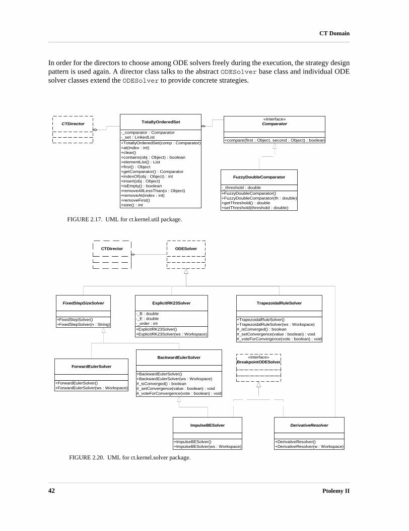
CT Domain

In order for the directors to choose among ODE solvers freely during the execution, the strategy designpattern is used again. A director class talks to the abstract ODESolver base class and individual ODEsolver classes extend the ODESolver to provide concrete strategies.

FIGURE 2.17. UML for ct.kernel.util package.

«Interface»Comparator

+compare(first : Object, second : Object) : boolean

FuzzyDoubleComparator

+FuzzyDoubleComparator()+FuzzyDoubleComparator(th : double)+getThreshold() : double+setThreshold(threshold : double)

-_threshold : double

TotallyOrderedSet

+TotallyOrderedSet(comp : Comparator)+at(index : int)+clear()+contains(obj : Object) : boolean+elementList() : List+first() : Object+getComparator() : Comparator+indexOf(obj : Object) : int+insert(obj : Object)+isEmpty() : boolean+removeAllLessThan(o : Object)+removeAt(index : int)+removeFirst()+size() : int

-_comparator : Comparator-_set : LinkedList

CTDirector

FIGURE 2.20. UML for ct.kernel.solver package.

FixedStepSizeSolver

+FixedStepSolver()+FixedStepSolver(n : String)

ForwardEulerSolver

+ForwardEulerSolver()+ForwardEulerSolver(ws : Workspace)

BackwardEulerSolver

+BackwardEulerSolver()+BackwardEulerSolver(ws : Workspace)#_isConverged() : boolean#_setConvergence(value : boolean) : void#_voteForConvergence(vote : boolean) : void

TrapezoidalRuleSolver

+TrapezoidalRuleSolver()+TrapezoidalRuleSolver(ws : Workspace)#_isConverged() : boolean#_setConvergence(value : boolean) : void#_voteForConvergence(vote : boolean) : void

ExplicitRK23Solver

+ExplicitRK23Solver()+ExplicitRK23Solver(ws : Workspace)

-_B : double-_E : double-_order : int

ImpulseBESolver

+ImpulseBESolver()+ImpulseBESolver(ws : Workspace)

ODESolverCTDirector

DerivativeResolver

+DerivativeResolver()+DerivativeResolver(w : Workspace)

«Interface»BreakpointODESolver

42 Ptolemy II

CT Domain

FIGURE 2.18. UML for ct.kernel package, actor related classes.

NumericalNonconvergeException

+NumericalNonconvergeException(detail : String)+NumericalNonconvergeException(obj : NamedObj, detail : String)+NumericalNonconvergeException(obj1 : NamedObj, obj2 : NamedObj, detail : String)

ptolemy.actor.TypedAtomicActor

CTBaseIntegrator

+CTBaseIntegrator(ca : TypedCompositeActor, name : String)+clearHistory()+getAuxVariables() : double[]+getDerivative() : double+getHistory(index : int) : double[]+getHistoryCapacity() : int+getState() : double+getTentativeState() : double+getValidHistoryCount() : int+setAuxVariables(index : int, value : double)+setHistoryCapacity(cap : int)+setTentativeDerivative(value : double)+setTentativeState(value : double)

+initialState : Parameter+input : TypedIOPort+output : TypedIOPort#_history : CTBaseIntegrator.History-_auxVariables : double[]-_initState : double-_state : double-_tentativeDerivative : double-_tentativeState : double

«Interface»CTDynamicActor

+emitTentativeOutput()

«Interface»CTStepSizeControlActor

+isThisStepAccurate() : boolean+predictedStepSize() : double+refinedStepSize() : double

«Interface»CTStatefulActor

+goToMarkedState()+markStates()

«Interface»CTEventGenerator

+hasCurrentEvent() : boolean

CTReceiver

+CTReceiver()+CTReceiver(container : IOPort)

+CONTINUOUS : CTReceiver.SignalType+DISCRETE : CTReceiver.SignalType+UNKNOWN : CTReceiver.SignalType

ptolemy.actor.Mailbox

«Interface»CTWaveformGenerator

«Interface»ptolemy.actor.Actor

ODESolver

+ODESolver()+ODESolver(w : Workspace)+ODESolver(w : Workspace, name : String)+getRound()+getHistoryCapacityRequirement() : int+getIntegratorAuxVariableCount() : int+incrementRound()+integratorFire(integ : CTBaseIntegrator)+integratorIsAccurate(integ : CTBaseIntegrator) : boolean+integratorPredictedStepSize(integ : CTBaseIntegrator) : double+resetRound()+resolveStates() : boolean

-_container : Director-_round : int

delegate

NamedObj CTDirector

ptolemy.actor.TypedCompositeActor

CTCompositeActor

+CTCompositeActor()+CTCompositeActor(ws : Workspace)+CTCompositeActor(ca : TypedCompositeActor, nm : String)

InvalidStateException

«throws»


CT Domain

FIGURE 2.19. UML for ct.kernel package, director related classes.

StaticSchedulingDirector

CTDirector

+CTDirector()+CTDirector(ws : Workspace)+CTDirector(ce : CompositeEntity, nm : String)+canBeInsideDirector() : boolean+canBeTopLevelDirector() : boolean+getBreakPoints() : TotallyOrderedSet+getCurrentODESolver() : ODESolver+getCurrentStepSize() : double+getInitialStepSize() : double+getIterationBeginTime() : double+getErrorTolerance() : double+getMaxIterations() : int+getMaxStepSize() : double+getMinStepSize() : double+getNextIterationTime() : double+getStartTime() : double+getStopTime() : double+getSuggestedNextStepSize() : double+getTimeResolution() : double+getValueResolution() : double+isBreakpointIteration() : boolean+isDiscretePhase() : boolean+produceOutput() : void+setCurrentStepSize(step : double)+setSuggestedNextStepSize(nextstep : double)+updateContinuousStates() : void

+errorTolerance : Parameter+initStepSize : Parameter+maxIteration : Parameter+maxStepSize : Parameter+minStepSize : Parameter+startTime : Parameter+stopTime : Parameter+synchronizeToRealTime : Parameter+timeResolution : Parameter+valueResolution : Parameter#_refireActors : LinkedList-_breakPoints : TotallyOrderedSet-_currentSolver : ODESolver-_currentStepSize : double-_suggestedNextStepSize : double

Scheduler

1..1

container

containee

ODESolver

CTMultiSolverDirector

+CTMultiSolverDirector()+CTMultiSolverDirector(ws : Workspace)+CTMultiSolverDirector(ce : CompositeEntity, nm : String)+getBreakpointSolver() : ODESolver+getODESolver() : ODESolver

+breakpointODESolver : Parameter+ODESolver : Parameter

CTScheduler

+CTScheduler()+CTScheduler(w : Workspace)+CTScheduler(container : Director, nm : String)+isDiscrete(actor : Actor) : boolean+isContinuous(actor : Actor) : boolean+predecessorList(actor : Actor) : List+successorList(actor : Actor) : List+signalTypeToString(signal : CTReceiver.SignalType) : String#_toArithmeticGraph(list : List) : DirectectedAcyclicGraph

+CONTINUOUS : CTReceiver.SignalTYpe+DISCRETE : CTReceiver.SignalType+UNKNOWN : CTReceiver.SignalType

CTEmbeddedDirector

+CTEmbeddedDirector()+CTEmbeddedDirector(ws : Workspace)+CTEmbeddedDirector(ce : CompositeEntity, nm : String)

-_outsideStepSize : double-_outsideTime : double

«Interface»CTTransparentDirector

+isThisStepAccurate() : boolean+predictedStepSize() : double+refinedStepSize() : double

CTMixedSignalDirector

+CTMixedSignalDirector()+CTMixedSignalDirector(ws : Workspace)+CTMixedSignalDirector(ce : CompositeEntity, nm : String)+getIterationEndTime() : double+getOutsideTime() : double#_catchup()#_markStates()#_rollback()

+runAheadLength : Parameter-_inEventPhase : boolean-_iterationEndTime : double-_knownGoodTime : double-_outsideTime : double

CTCompositeActor

CTSchedule

+CTSchedule()

+CONTINUOUS_ACTORS : int+DISCRETE_ACTORS : int+DYNAMIC_ACTORS : int+EVENT_GENERATORS : int+OUTPUT_ACTORS : int+OUTPUT_STEP_SIZE_CONTROL_ACTORS : int+STATE_STEP_SIZE_CONTROL_ACTORS : int+STATE_TRANSITION_ACTORS : int+WAVEFORM_GENERATORS : int

44 Ptolemy II

CT Domain

2.8.3 Scheduling

This section and the following three sections provide technical details and design decisions madein the implementation of the CT domain. These details are only necessary if the readers want to imple-ment new directors or ODE solvers.

In general, simulating a continuous-time system (3)-(5) by a time-marching ODE solver involvesthe following execution steps:

1. Given the state of the system at time points , if the current integration step size is , i.e. , compute the new state using the numerical integration algorithms. During the application of an integration algorithm, each evaluation of the f(a, b, t) function is achieved by the following sequence:

• Integrators emit tokens corresponding to a;• Source actors emit tokens corresponding to b;• The current time is set to t;• The tokens are passed through the topology (in a data-driven way) until they reach the integrators

again. The returned tokens are .

2. After the new state is computed, test whether this step is successful. Local truncation error and unpredictable breakpoints are the issues to be concerned with, since those could lead to an unsuc-cessful step.

3. If the step is successful, predict the next step size. Otherwise, reduce the step size and try again.Due to the signal-flow representation of the system, the numerical ODE solving algorithms are imple-mented as actor firings and token passings under proper scheduling.

The scheduler partitions a CT system into two clusters: the state transition cluster and the outputcluster. In a particular system, these clusters may overlap.

The state transition cluster includes all the actors that are in the signal flow path for evaluating thef function in (3). It starts from the source actors and the outputs of the integrators, and ends at theinputs of the integrators. In other words, integrators, and in general dynamic actors, are used to breakcausality loops in the model. A topological sort of the cluster provides an enumeration of actors in theorder of their firings. This enumeration is called the state transition schedule. After the integrators pro-duce tokens representing , one iteration of the state transition schedule gives the tokens representing

back to the integrators. The output cluster consists of actors that are involved in the evaluation of the output map g in (4).

It is also similarly sorted in topological order. The output schedule starts from the source actors and theintegrators, and ends at the sink actors.

For example, for the system shown in figure 2.3, the state transition schedule isU-G1-G2-G3-A

where the order of G1, G2, and G3 are interchangeable. The output schedule is G4-Y

The event generating schedule is empty.A special situation that must be taken care of is the firing order of a chain of integrators, as shown

in figure 2.21. For the implicit integration algorithms, the order of firings determines two distinct kindsof fixed point iterations. If the integrators are fired in the topological order, namely in ourexample, the iteration is called the Gauss-Seidel iteration. That is, always uses the new guess from

xt0…xtn 1–

t0…tn 1–h tn tn 1– h+= xtn

x·x a=

f a b t, ,( )=

xtn

xtx· t f xt u t( ) t,,( )=

x1 x2→x2


CT Domain

in this iteration for its new guess. On the other hand, if they are fired in the reverse topologicalorder, the iteration is called the Gauss-Jacobi iteration, where uses the tentative output from inthe last iteration for its new estimation. The two iterations both have their pros and cons, which arethoroughly discussed in [115]. Gauss-Seidel iteration is considered faster in the speed of convergencethan Gauss-Jacobi. For explicit integration algorithms, where the new states are calculated solelyfrom the history inputs up to , the integrators must be fired in their reverse topological order. Forsimplicity, the scheduler of the CT domain, at this time, always returns the reversed topological orderof a chain of integrators. This order is considered safe for all integration algorithms.

2.8.4 Controlling Step Sizes

Choosing the right time points to approximate a continuous time system behavior is one of themajor tasks of simulation. There are three factors that may impact the choice of the step size. • Error control. For all integration algorithms, the local error at time is defined as a vector norm

(say, the 2-norm) of the difference between the actual solution and the approximation calculated by the integration method, given that the last step is accurate. That is, assuming

then

. (30)

It can be shown that by carefully choosing the parameters in the integration algorithms, the localerror is approximately of the p-th order of the step size, where p, an integer closely related to thenumber of f function evaluations in one integration step, is called the order of the integration algo-rithm, i.e. . Therefore, in order to achieve an accurate solution, the step sizeshould be chosen to be small. But on the other hand, small step sizes means long simulation time.In general, the choice of step size reflects the trade-off between speed and accuracy of a simula-tion.

• Convergence. The local contraction mapping theorem (Theorem 2 in Appendix A) shows that for implicit ODE solvers, in order to find the fixed point at , the map in (15) must be a (local) contraction map, and the initial guess must be within an ball (the contraction radius) of the solu-tion. It can be shown that can be made contractive if the step size is small enough. (The choice of the step size is closely related to the Lipschitz constant). So the general approach for resolving the fixed point is that if the iterating function does not converge at one step size, then reduce the step size by half and try again.

• Discontinuity. At discontinuous points, the derivatives of the signals are not continuous, so the integration formula is not applicable. That means the discontinuous points can not be crossed by one integration step. In particular, suppose the current time is t and the intended next time point is t+h. If there is a discontinuous point at , where , then the next step size should be reduced to . For a predictable breakpoint, the director can adjust the step size accordingly before starting an integration step. However for an unpredictable breakpoint, which is reported “missed” after an integration step, the director should be able to discard its last step and restart

td∫ td∫x1 x2

x2·

x1·

FIGURE 2.21. A chain of integrators.

x1x2 x1

xtnx· tn 1–

tnx tn( ) xtn

xtn 1–x tn 1–( )=

Etnxtn

x tn( )–=

EtnO tn tn 1––( )p( )∼

tn FI ( )ε

FI ( )

FI ( )

t δ+ δ h<t δ+

46 Ptolemy II

CT Domain

with a smaller step size to locate the actual discontinuous point.

Notice that convergence and accuracy concerns only apply to some ODE solvers. For example,explicit algorithms do not have the convergence problem, and fixed step size algorithms do not havethe error control capability. On the other hand, discontinuity control is a generic feature that is inde-pendent on the choice of ODE solvers.

2.8.5 Mixed-Signal Execution

DE inside CT.

Since time advances monotonically in CT and events are generated chronologically, the DE com-ponent receives input events monotonically in time. In addition, a composition of causal DE compo-nents is causal [82], so the time stamps of the output events from a DE component are always greaterthan or equal to the global time. From the view point of the CT system, the events produced by a DEcomponent are predictable breakpoints.

Note that in the CT model, finding the numerical solution of the ODE at a particular time is seman-tically an instantaneous behavior. During this process, the behavior of all components, including thoseimplemented in a DE model, should keep unchanged. This implies that the DE components should notbe executed during one integration step of CT, but only between two successive CT integration steps.

CT inside DE.

When a CT component is contained in a DE system, the CT component is required to be causal,like all other components in the DE system. Let the CT component have local time , when it receivesan input event with time stamp . Since time is continuous in the CT model, it will execute from itslocal time , and may generate events at any time greater or equal to . Thus we need

(31)

to ensure causality. This means that the local time of the CT component should always be greater thanor equal to the global time whenever it is executed.

This ahead-of-time execution implies that the CT component should be able to remember its paststates and be ready to rollback if the input event time is smaller than its current local time. The state itneeds to remember is the state of the component after it has processed an input event. Consequently,the CT component should not emit detected events to the outside DE system before the global timereaches the event time. Instead, it should send a pure event to the DE system at the event time, and waituntil it is safe to emit it.

2.8.6 Hybrid System Execution

Although FSM is an untimed model, its composition with a timed model requires it to transfer thenotion of time from its external model to its internal model. During continuous evolution, the system issimulated as a CT system where the FSM is replaced by the continuous component refining the currentFSM state. After each time point of CT simulation, the triggers on the transitions starting from the cur-rent FSM state are evaluated. If a trigger is enabled, the FSM makes the corresponding transition. Thecontinuous dynamics of the destination state is initialized by the actions on the transition. The simula-tion continues with the transition time treated as a breakpoint.

tτ

t t

t τ≥


CT Domain

Appendix A: Brief Mathematical Background

Theorem 1. [Existence and uniqueness of the solution of an ODE] Consider the initialvalue ODE problem

. (32)

If f satisfies the conditions:

1. [Continuity Condition] Let D be the set of possible discontinuity points; it may be empty. For each

fixed and , the function in (32) is continuous. And , the

left-hand and right-hand limit and are finite.

2. [Lipschitz Condition] There is a piecewise continuous bounded function : , where is the set of non-negative real numbers, such that

. (33)

Then, for each initial condition there exists a unique continuous function

such that,

(34)

and

. (35)

This function is called the solution through of the ODE (32).

Theorem 2. [Contraction Mapping Theorem.] If is a local contraction map at

x with contraction radius , then there exists a unique fixed point of F within the ball centered at x.

I.e. there exists a unique , , such that . And , the

sequence

(36)

converges to .

x· f x t,( )x t0( ) x0

==

x ℜn∈ u ℜm∈ f:ℜ\ D ℜn→ τ∀ D∈

f x u τ-, ,( ) f x u τ+, ,( )

k ℜ ℜ +→ ℜ+

t ℜ ζ ξ ℜnu ℜm∈∀,∈,∀,∈∀

f ξ u t, ,( ) f ζ u t, ,( )– k t( ) ξ ζ–≤

t0 x0,( ) ℜ ℜn×⊆

ψ: ℜ ℜn→

ψ t0( ) x0=

ψ· t( ) f ψ t( ) u t( ) t, ,( ) t ℜ\D∈∀=

ψ t( ) t0 x0,( )

F:ℜn ℜn→ε ε

σ ℜn∈ σ x– ε≤ σ F σ( )= σ0 ℜn σ0 x– ε≤,∈∀

σ1 F σ0( ), σ2 F σ1( ), σ3 F σ2( ), …= = =

σ

48 Ptolemy II

Heterogeneous Concurrent Modeling and Desi

3
SDF Domain
Author: Steve NeuendorfferContributor: Brian Vogel

3.1 Purpose of the Domain

The synchronous dataflow (SDF) domain is useful for modeling simple dataflow systems withoutcomplicated flow of control, such as signal processing systems. Under the SDF domain, the executionorder of actors is statically determined prior to execution. This results in execution with minimal over-head, as well as bounded memory usage and a guarantee that deadlock will never occur. This domain isspecialized, and may not always be suitable. Applications that require dynamic scheduling could usethe process networks (PN) domain instead, for example.

3.2 Using SDF

There are four main issues that must be addressed when using the SDF domain:• Deadlock• Consistency of data rates• The value of the iterations parameter• The granularity of execution

This section will present a short description of these issues. For a more complete description, seesection 3.3.

3.2.1 Deadlock

Consider the SDF model shown in figure 3.1. This actor has a feedback loop from the output of theAddSubtract actor back to its own input. Attempting to run the model results in the exception shown atthe right in the figure. The director is unable to schedule the model because the input of the AddSub-tract actor depends on data from its own output. In general, feedback loops can result in such condi-

gn 49

SDF Domain

tions.The fix for such deadlock conditions is to use the SampleDelay actor, shown highlighted in figure

3.2. This actor injects into the feedback loop an initial token, the value of which is given by the initia-lOutputs parameter of the actor. In the figure, this parameter has the value {0}. This is an array with asingle token, an integer with value 0. A double delay with initial values 0 and 1 can be specified usinga two element array, such as {0, 1}.

It is important to note that it is occasionally necessary to add a delay that is not in a feedback loopto match the delay of an input with the delay around a feedback loop. It can sometimes be tricky to seeexactly where such delays should be placed without fully considering the flow of the initial tokensdescribed above.

FIGURE 3.1. An SDF model that deadlocks.

FIGURE 3.2. The model of figure 3.1 corrected with an instance of SampleDelay in the feedback loop.

50 Ptolemy II

SDF Domain

3.2.2 Consistency of data rates

Consider the SDF model shown in figure 3.3. The model is attempting to plot a sinewave and itsdownsampled counterpart. However, there is an error because the number of tokens on each channel ofthe input port of the plotter can never be made the same. The DownSample actor declares that it con-sumes 2 tokens using the tokenConsumptionRate parameter of its input port. Its output port similarlydeclares that it produces only one token, so there will only be half as many tokens being plotted fromthe DownSample actor as from the Sinewave.

The fixed model is shown in figure 3.4, which uses two separate plotters. When the model is exe-cuted, the plotter on the bottom will fire twice as often as the plotter on the top, since it must consumetwice as many tokens. Notice that the problem appears because one of the actors (in this case, theDownSample actor) produces or consumes more than one token on one of its ports. One easy way toensure rate consistency is to use actors that only produce and consume one token at a time. This specialcase is known as homogeneous SDF. Note that actors like the SequencePlotter which do not specifyrate parameters are assumed to be homogeneous. For more specific information about the rate parame-

FIGURE 3.3. An SDF model with inconsistent rates.

FIGURE 3.4. Figure 3.3 modified to have consistent rates.


SDF Domain

ters and how they are used for scheduling, see section 3.3.1.

3.2.3 How many iterations?

Another issue when using the SDF domain concerns the value of the iterations parameter of theSDF director. In homogeneous models one token is usually produced for every iteration. However,when token rates other than one are used, more than one interesting output value may be created foreach iteration. For example, consider figure 3.5 which contains a model that plots the Fast FourierTransform of the input signal. The important thing to realize about this model is that the FFT actordeclares that it consumes 256 tokens from its input port and produces 256 tokens from its output port,corresponding to an order 8 FFT. This means that only one iteration is necessary to produce all 256values of the FFT.

Contrast this with the model in figure 3.6. This model plots the individual values of the signal.Here 256 iterations are necessary to see the entire input signal, since only one output value is plotted ineach iteration.

3.2.4 Granularity

The granularity of execution of an SDF model is determined by solving a set of equations deter-mined by declared data rates of actors, and the connections between actors. As mentioned in the previ-ous section, this schedule may involve a small or large number of firings of each actor, depending onthe relative data rates of the actors. Generally, the smallest possible valid schedule, corresponding tothe smallest granularity of execution, is the most interesting. However, there are some instances when

FIGURE 3.5. A model that plots the Fast Fourier Transform of a signal. Only one iteration must be executed to plot all 256 values of the FFT, since the FFT actor produces and consumes 256 tokens each firing.

FIGURE 3.6. A model that plots the values of a signal. 256 iterations must be executed to plot the entire sig-nal.

52 Ptolemy II

SDF Domain

this is not the case. In such cases the vectorizationFactor parameter of the SDF director can be used toscale up the granularity of the schedule. A vectorizationFactor of 2 implies that each actor is firedtwice as many times as in the normal schedule.

One example when this might be useful is when modeling block data processing. For instance, wemight want to build a model of a signal processing system that filters blocks of 40 samples at a timeusing an FIR filter. Such an actor could be written in Java, or it could be built as a hierarchical SDFmodel, using a single sample FIR filter, as shown in Figure 3.7. The vectorizationFactor parameter ofthe director is set to 40. Here, each firing of the SDF model corresponds to 40 firings of the single sam-ple FIR filter.

Another useful time to increase the level of granularity is to allow vectorized execution of actors.Some actors override the iterate() method to allow optimized execution of several consecutive firings.Increasing the granularity of an SDF model can provide more opportunities for the SDF director toperform this optimization, especially in models that do not have fine-grained feedback.

3.3 Properties of the SDF domain

SDF is an untimed model of computation. All actors under SDF consume input tokens, performtheir computation and produce outputs in one atomic operation. If an SDF model is embedded within atimed model, then the SDF model will behave as a zero-delay actor.

In addition, SDF is a statically scheduled domain. The firing of a composite actor corresponds to asingle iteration of the contained(3.3.1) model. An SDF iteration consists of one execution of the pre-calculated SDF schedule. The schedule is calculated so that the number of tokens on each relation isthe same at the end of an iteration as at the beginning. Thus, an infinite number of iterations can beexecuted, without deadlock or infinite accumulation of tokens on each relation.

Execution in SDF is extremely efficient because of the scheduled execution. However, in order toexecute so efficiently, some extra information must be given to the scheduler. Most importantly, thedata rates on each port must be declared prior to execution. The data rate represents the number oftokens produced or consumed on a port during every firing1. In addition, explicit data delays must beadded to feedback loops to prevent deadlock. At the beginning of execution, and any time these datarates change, the schedule must be recomputed. If this happens often, then the advantages of scheduledexecution can quickly be lost.

1. This is known as multirate SDF, where arbitrary rates are allowed. Not to be confused with homogeneous SDF, where the data rates are fixed to be one.

FIGURE 3.7. A model that implements a block FIR filter. The vectorizationFactor parameter of the director is set to the size of the block.


SDF Domain

3.3.1 Scheduling

The first step in constructing the schedule is to solve the balance equations [87]. These equationsdetermine the number of times each actor will fire during an iteration. For example, consider the modelin figure 3.8. This model implies the following system of equations, where ProductionRate and Con-sumptionRate are declared properties of each port, and Firings is a property of each actor that will besolved for:

Firings(A) × ProductionRate(A1) = Firings(B) × ConsumptionRate(B1)

Firings(A) × ProductionRate(A2) = Firings(C) × ConsumptionRate(C1)

Firings(C) × ProductionRate(C2) = Firings(B) × ConsumptionRate(B2)

These equations express constraints that the number of tokens created on a relation during an iterationis equal to the number of tokens consumed. These equations usually have an infinite number of lin-early dependent solutions, and the least positive integer solution for Firings is chosen as the firing vec-tor, or the repetitions vector.

The second step in constructing an SDF schedule is dataflow analysis. Dataflow analysis ordersthe firing of actors, based on the relations between them. Since each relation represents the flow ofdata, the actor producing data must fire before the consuming actor. Converting these data dependen-cies to a sequential list of properly scheduled actors is equivalent to topologically sorting the SDFgraph, if the graph is acyclic1. Dataflow graphs with cycles cause somewhat of a problem, since suchgraphs cannot be topologically sorted. In order to determine which actor of the loop to fire first, a datadelay must be explicitly inserted somewhere in the cycle. This delay is represented by an initial tokencreated by one of the output ports in the cycle during initialization of the model. The presence of thedelay allows the scheduler to break the dependency cycle and determine which actor in the cycle to firefirst. In Ptolemy II, the initial token (or tokens) can be sent from any port, as long as the port declaresan tokenInitProduction property. However, because this is such a common operation in SDF, the Sam-pleDelay actor (see section 3.5) is provided that can be inserted in a feedback loop to break the cycle.Cyclic graphs not properly annotated with delays cannot be executed under SDF. An example of acyclic graph properly annotated with a delay is shown in figure 3.9.

In some cases, a non-zero solution to the balance equations does not exist. Such models are said to

1. Note that the topological sort does not correspond to a unique total ordering over the actors. Furthermore, espe-cially in multirate models it may be possible to interleave the firings of actors that fire more than once. This can result in many possible schedules that represent different performance trade-offs. We anticipate that future schedulers will be implemented to take advantage of these trade-offs. For more information about these trade-offs, see [47].

E0

D1: SDF director

A1

AA2

C1C

C2

B1

BB2

FIGURE 3.8. An example SDF model.

54 Ptolemy II

SDF Domain

be inconsistent, and cannot be executed under SDF. Inconsistent graphs inevitably result in eitherdeadlock or unbounded memory usage for any schedule. As such, inconsistent graphs are usually bugsin the design of a model. However, inconsistent graphs can still be executed using the PN domain, ifthe behavior is truly necessary. Examples of consistent and inconsistent graphs are shown in figure3.10.

3.3.2 Hierarchical Scheduling

So far, we have assumed that the SDF graph is not hierarchical. The simplest way to schedule ahierarchical SDF model is flatten the model to remove the hierarchy, and then schedule the model as

E4

2

1 2

1 1

2

D1: SDF director

AB

C

FIGURE 3.9. A consistent cyclic graph, properly annotated with delays. A one token delay is represented by a black circle. Actor C is responsible for setting the tokenInitProduction parameter on its output port, and cre-ating the two tokens during initialization. This graph can be executed using the schedule A, A, B, C, C.

E1

D1: SDF director

A1

AA2

C1C

C2

B1

BB2

1

1

1

1

22

E2

D1: SDF director

A1

AA2

C1C

C2

B1

BB2

1

1

1

1

21

FIGURE 3.10. Two models, with each port annotated with the appropriate rate properties. The model on the top is consistent, and can be executed using the schedule A, A, C, B, B. The model on the bottom is inconsis-tent because tokens will accumulate between ports C2 and B2.


SDF Domain

usual. This technique allows the most efficient schedule to be constructed for a model, and avoids cer-tain composability problems when creating hierarchical models. In Ptolemy II, a model created using atransparent composite actor to define the hierarchy is scheduled in exactly this way.

Ptolemy II also supports a stronger version of hierarchy, in the form of opaque composite actors. Inthis case, the hierarchical actor appears to be no different from the outside than an atomic actor with nohierarchy. The SDF domain does not have any information about the contained model, other than therate parameters that may be specified on the ports of the composite actor. The SDF domain is designedso that it automatically sets the rates of external ports when the schedule is computed. Most otherdomains are designed (conveniently enough) so that their models are compatible with default rateproperties assumed by the SDF domain. For a complete description of these defaults, see the descrip-tion of the SDFScheduler class in section 3.4.2.

3.3.3 Hierarchically Heterogeneous Models

An SDF model can generally be embedded in any other domain. However, SDF models are unlikemost other hierarchical models in that they often require multiple inputs to be present. When buildingone SDF model inside another SDF model, this is ensured by the containing SDF model because of theway the data rate parameters are set as described in the previous section. For most other domains, theSDF director will check how many tokens are available on its input ports and will refuse firing (byreturning false in prefire()) until enough data is present for an entire iteration to complete.

3.4 Software Architecture

The SDF kernel package implements the SDF model of computation. The structure of the classesin this package is shown in figure 3.11.

3.4.1 SDF Director

The SDFDirector class extends the StaticSchedulingDirector class. When an SDF director is cre-ated, it is automatically associated with an instance of the default scheduler class, SDFScheduler. Thisscheduler is intended to be relatively fast, but not designed to optimize for any particular performancegoal. The SDF director does not currently restrict the schedulers that may be used with it. For moreinformation about SDF schedulers, see section 3.4.2.

The director has a parameter, iterations, which determines a limit on the number of times thedirector wishes to be fired1. After the director has been fired the given number of times, it will alwaysreturn false in its postfire() method, indicating that it does not wish to be fired again. The iterationsparameter must contain an integer value. The default value is an IntToken with value 0. A non-positiveinteger indicates that there is no preset limit for the number of times the director will fire. Users willlikely specify a positive value in the director of the toplevel composite actor as the number of topleveliterations of the model.

The SDF director also has a vectorizationFactor parameter that can be used to request vectorizedexecution of a model. This parameter increases the granularity of the executed schedule so that thedirector fires each actor vectorizationFactor times of the normal. The vectorizationFactor parametermust contain a positive integer value. The default value is an IntToken with value one, indicating thatno vectorization should be done. Changing this parameter changes the meaning of an embedded SDF

1. This parameter acts similarly to the Time-to-Stop parameter in Ptolemy Classic.

56 Ptolemy II

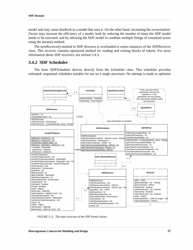
SDF Domain

model and may cause deadlock in a model that uses it. On the other hand, increasing the vectorization-Factor may increase the efficiency of a model, both by reducing the number of times the SDF modelneeds to be executed, and by allowing the SDF model to combine multiple firings of contained actorsusing the iterate() method.

The newReceiver() method in SDF directors is overloaded to return instances of the SDFReceiverclass. This receiver contains optimized method for reading and writing blocks of tokens. For moreinformation about SDF receivers, see section 3.4.3.

3.4.2 SDF Scheduler

The basic SDFScheduler derives directly from the Scheduler class. This scheduler providesunlooped, sequential schedules suitable for use on a single processor. No attempt is made to optimize

FIGURE 3.11. The static structure of the SDF kernel classes.

TypedIOPort

SDFScheduler

+SDFScheduler()+SDFScheduler(container : Director, name : String)+SDFScheduler(w : Workspace)+getFiringCount(entity : Entity) : int+getTokenConsumptionRate(p : IOPort) : int+getTokenInitProduction(p : IOPort) : int+getTokenProductionRate(p : IOPort)

SDFDirector

+SDFDirector()+SDFDirector(w : Workspace)+SDFDirector(c : CompositeEntity, name : String)

iterations : int vectorizationFactor : int

1..1

1..1

SDFReceiver

+SDFReceiver()+SDFReceiver(size : int)+SDFReceiver(container : IOPort)+SDFReceiver(container : IOPort, size : int)+get(offset : int) : Token+getCapacity() : int+getHistoryCapacity() : int+historyElements() : Enumeration+historySize() : int+setCapacity(capacity : int)+setHistoryCapacity(capacity : int)+size() : int

ArrayFIFOQueue

+ArrayFIFOQueue()+ArrayFIFOQueue(size : int)+ArrayFIFOQueue(container : Nameable)+ArrayFIFOQueue(container : Nameable, size : int)+ArrayFIFOQueue(model : ArrayFIFOQueue)+elementList() : Llist+elements() : Enumeration+get(offset : int)+getCapacity() : int+getContainer() : Nameable+getHistoryCapacity() : int+historyElements() : Enumeration+historySize() : int+isEmpty() : boolean+isFull() : boolean+put(o : Object)+putArray(o : Object[])+putArray(array : object[], count : int)+setCapacity(capacity : int)+setContainer(container : Nameable)+setHistoryCapacity(capacity : int)+size() : int+take() : Object+takeArray(o : Object[])+takeArray(o : object [], count : int)

+INFINITE_CAPACITY : int+DEFAULT_CAPACITY : int+STARTING_ARRAYSIZE : int+DEFAULT_HISTORY_CAPACITY : int-_container : Nameable-_queuearray : Object[]-_historyList : LinkedList

1..1

1..1

0..n

1..1

Receiver

+get() : Token+getArray(length : int) : Token[]+getContainer() : IOPort+hasRoom() : boolean+hasRoom(count : int) : boolean+hasToken() : boolean+hasToken(count : int) : boolean+put(t : Token)+putArray(tokens : Token [], length : int)+setContainer(port : IOPort)

SDFIOPort

+SDFIOPort(c : ComponentEntity, name : String)+getTokenConsumptionRate() : int+getTokenInitProduction() : int+getTokenProductionRate() : int+setTokenConsumptionRate(rate : int)+setTokenInitProduction(rate : int)+setTokenProductionRate(rate : int)

+tokenConsumptionRate : int+tokenInitProduction : int+tokenProductionRate : int

TypedAtomicActor

0..n

1..1

Ports may have theseparameters, but are not

required to. If theparameters are not present,

then appropriate default valuesare assumed.


uses parameters to schedule

creates

Scheduler

+getSchedule() : Schedule+schedule() : Enumeration

creates

actor.AbstractReceiver


SDF Domain

the schedule by minimizing data buffer sizes, minimizing the size of the schedule, or detecting paral-lelism to allow execution on multiple processors. We anticipate that more elaborate schedulers capableof these optimizations will be added in the future.

The scheduling algorithm is based on the simple multirate algorithm in [87]. Currently, only singleprocessor schedules are supported. The multirate scheduling algorithm relies on the actors in the sys-tem to declare the data rates of each port. The data rates of ports are specified using three parameterson each port named tokenConsumptionRate, tokenProductionRate, and tokenInitProduction. The pro-duction parameters are valid only for output ports, while the consumption parameter is valid only forinput ports. If a parameter exists that is not valid for a given port, then the value of the parameter mustbe zero, or the scheduler will throw an exception. If a valid parameter is not specified when the sched-uler runs, then default values of the parameters will be assumed, however the parameters are not thencreated1.

After scheduling, the SDF scheduler will set the rate parameters on any external ports of the com-posite actor. This allows a containing actor, which may represent an SDF model, to properly schedulethe contained model, as long as the contained model is scheduled first. To ensure this, the SDF directorforces the creation of the schedule after initializing all the actors in the model. The SDF scheduler alsosets attributes on each relation that give the maximum buffer size of the relation. This can be usefulfeedback for analyzing deadlocks, or for visualization.This mechanism is illustrated in the sequencediagram in figure 3.12.

SDF graphs should generally be connected. If an SDF graph is not connected, then there is someconcurrency between the disconnected parts that is not captured by the SDF rate parameters. In suchcases, another model of computation (such as process networks) should be used to explicitly specifythe concurrency. As such, the SDF scheduler by default disallows disconnected graphs, and will throwan exception if you attempt to schedule such a graph. However, sometimes it is useful to avoid intro-ducing another model of computation, or to allow dynamic modifications to an executing model. Bysetting the allowDisconnectedGraphs parameter of the SDF director to true, the scheduler will assumea default notion of concurrency between different parts of a model. Each disconnected ‘island’ will bescheduled independently, and an overall schedule created that includes one execution of the schedulefor each island.

Multiports. Notice that it is impossible to set a rate parameter on individual channels of a port. This isintentional, and all the channels of an actor are assumed to have the same rate. For example, when theAddSubtract actor fires under SDF, it will consume exactly one token from each channel of its inputplus port, consume one token from each channel of its minus port, and produce one token the singlechannel of its output port. Notice that although the domain-polymorphic adder is written to be moregeneral than this (it will consume up to one token on each channel of the input port), the SDF sched-uler will ensure that there is always at least one token on each input port before the actor fires.

Dangling ports. All channels of a port are required to be connected to a remote port under the SDFdomain. A regular port that is not connected will always result in an exception being thrown by thescheduler. However, the SDF scheduler detects multiports that are not connected to anything (and thushave zero width). Such ports are interpreted to have no channels, and will be ignored by the SDFscheduler.

1. The assumed values correspond to a homogeneous actor with no data delay. Input ports are assumed to have a consumption rate of one, output ports are assumed to have a production rate of one, and no tokens are produced during initialization.

58 Ptolemy II

SDF Domain

3.4.3 SDF ports and receivers

Unlike most domains, multirate SDF systems tend to produce and consume large blocks of tokensduring each firing. Since there can be significant overhead in data transport for these large blocks, SDFreceivers are optimized for sending and receiving a block of tokens en masse.

The SDFReceiver class implements the Receiver interface. Instead of using the FIFOQueue classto store data, which is based on a linked list structure, SDF receivers use the ArrayFIFOQueue class,which is based on a circular buffer. This choice is much more appropriate for SDF, since the size of thebuffer is bounded, and can be determined statically1.

The SDFIOPort class extends the TypedIOPort class. It exists mainly for convenience when creat-ing actors in the SDF domain. It provides convenience methods for setting and accessing the rateparameters used by the SDF scheduler.

1. Although the buffer sizes can be statically determined, the current mechanism for creating receivers does not easily support it. The SDF domain currently relies on the buffer expanding algorithm that the ArrayFIFOQueue uses to implement circular buffers of unbounded size. Although there is some overhead during the first iteration, the overhead is minimal during subsequent iterations (since the buffer is guaranteed never to grow larger).

FIGURE 3.12. The sequence of method calls during scheduling of a hierarchical model.

a:CompositeActor

a.d:SDFDirector

s1:SDFScheduler

initialize()

a.b:CompositeActor

a.b.d:SDFDirector

s2:SDFScheduler

initialize()

initialize()

sc1:Schedule

a.b.p:IOPort

setRates

getSchedule()

sc2:Schedule

a.p:IOPort

getRates

getSchedule()

setRates


SDF Domain

3.4.4 ArrayFIFOQueue

The ArrayFIFOQueue class implements a first in, first out (FIFO) queue by means of a circulararray buffer1. Functionally it is very similar to the FIFOQueue class, although with different enqueueand dequeue performance. It provides a token history and an adjustable, possibly unspecified, boundon the number of tokens it contains.

If the bound on the size is specified, then the array is exactly the size of the bound. In other words,the queue is full when the array becomes full. However, if the bound is unspecified, then the circularbuffer is given a small starting size and allowed to grow. Whenever the circular buffer fills up, it iscopied into a new buffer that is twice the original size.

3.5 Actors

Most domain-polymorphic actors can be used under the SDF domain. However, actors that dependon a notion of time may not work as expected. For example, in the case of a TimedPlotter actor, all datawill be plotted at time zero when used in SDF. In general, domain-polymorphic actors (such asAddSubtract) are written to consume at most one token from each input port and produce exactly onetoken on each output port during each firing. Under SDF, such an actor will be assumed to have a rateof one on each port, and the actor will consume exactly one token from each input port during each fir-ing. There is one actor that is normally only used in SDF: the SampleDelay actor. This actor is pro-vided to make it simple to build models with feedback, by automatically handling thetokenInitProduction parameter and providing a way to specify the tokens that are created.

SampleDelayPorts: input (Token), output (Token).Parameters: initialOutputs (ArrayToken).

During initialization, create a token on the output for each token in the initialOutputs array. During each firing, consume one token on the input and produce the same token on the output.

1. Adding an array of objects to an ArrayFIFOQueue is implemented using the java.lang.system.arraycopy method. This method is capable of safely removing certain checks required by the Java language. On most Java implementations, this is significantly faster than a hand coded loop for large arrays. However, depending on the Java implementation it could actually be slower for small arrays. The cost is usually negligible, but can be avoided when the size of the array is small and known when the actor is written.

60 Ptolemy II


4
FSM Domain
Authors: Xiaojun LiuEdward A. LeeHaiyang Zheng

4.1 Introduction

Finite state machines (FSMs) have been used extensively in designing sequential control logic.There are two major reasons behind their use. First, FSMs are a very intuitive way to capture controllogic and make it easier to communicate a design. Second, FSMs have been the subject of a long his-tory of research work. Many formal analysis and verification methods have been developed for them.

In their simple flat form, FSM models have a key weakness: the number of states in an FSM modelcan get quite large even for a moderately complex system. Such models quickly become chaotic andincomprehensible when one tries to model a system having many concurrent activities. The problemcan be solved by introducing hierarchical organization into FSM models and using them in combina-tion with concurrency models. David Harel first used this approach when he introduced the Statechartsformalism [52].

The Statecharts formalism extends the conventional FSM model in three aspects: hierarchicaldecomposition of states, concurrent composition of FSMs in a synchronous-reactive fashion, and abroadcast communication mechanism between concurrent components. While how these extensions fittogether was not completely specified in [52], Harel’s work stimulated a lot of interest in the approach.Consequently, there is a proliferation of variants of the Statecharts formalism [12], each proposing adifferent way to make the extensions fit into a monolithic model. Unfortunately, in all these variantsFSM is combined with a particular concurrency model. The applicability of the resulting models isoften limited.

Based on the Ptolemy philosophy of hierarchical composition of heterogeneous models of compu-tation, the *charts1 formalism [47] allows embedding hierarchical FSMs within a variety of concur-rency models. If tight synchronization is possible and desirable, then FSMs can be composed by thesynchronous-reactive model. If the system has a global notion of time and components communicate

esign 61

FSM Domain

by time-stamped events, then FSMs can be composed by the discrete-event model. The rest of thischapter focuses on how the FSM domain in Ptolemy II supports the *charts formalism.

4.2 Building FSMs in Vergil

An FSM model is contained by an instance of FSMActor. The FSM model reacts to inputs to theFSM actor by making state transitions. Actions such as sending tokens to the output ports of the FSMactor can be associated with state transitions. In this section, we show how to construct and run amodel with an FSM actor in Vergil.

4.2.1 Alternate Mark Inversion Coder

Alternate Mark Inversion (AMI) is a simple digital transmission technique that encodes a bitstream on a signal line as shown below:

The 0 bits are transmitted with voltage zero. The 1 bits are transmitted alternately with positive andnegative voltages. On average, the resulting waveform will have no DC component.

We can model an AMI coder with a two-state FSM shown in figure 4.2. To construct a Ptolemy IImodel containing this coder, follow these steps:

1. Start Vergil, open a graph editor by selecting File -> New -> Graph Editor.

2. From MoreLibraries/Automata in the palette on the left, drag an FSM actor to the graph. Rename the FSM actor AMICoder.

3. Right click on AMICoder, select Configure Ports. Add an input port with name in and an output port with name out to AMICoder.

4. Right click on AMICoder, select Look Inside. This will open an FSM editor for AMICoder. Note that the ports of AMICoder are placed at the upper left corner of the graph panel.

5. From the palette on the left, drag a state to the graph, rename it Positive. Drag another state to the graph, rename it Negative.

6. Control-drag from the Positive state to the Negative state to create a transition.

7. Double click on the transition. This will bring up the dialog box shown in figure 4.1 for editing the parameters of the transition.

8. Set guardExpression to in == 1, and outputActions to out = 1.

9. Create a transition from the Positive state back to itself with guard expression in == 0 and output action out = 0.

1. Pronounced “starcharts.” The star represents a wildcard that can be interpreted as matching multiple concur-rency models.

0 0 0 0 0 01 1 1 1 1 1 1+V

-V0

62 Ptolemy II

FSM Domain

10. Create a transition from the Negative state back to itself with guard expression in == 0 and out-put action out = 0.

11. Create a transition from the Negative state to the Positive state with guard expression in == 1 and output action out = -1.

12. Right click on the background of the graph panel. Select Configure from the context menu. This will bring up the dialog box for editing parameters of AMICoder. Set initialStateName to Posi-tive.

13. The construction of AMICoder is complete. It will look like what is shown in figure 4.2.

14. Return to the graph editor opened in step 1.

15. Drag a Pulse actor (from Actors/Sources/SequenceSources), a SequencePlotter (from Actors/Sinks/SequenceSinks), and an SDF director (from Directors) to the graph.

16. Connect the actors as shown in figure 4.3.

FIGURE 4.1. The dialog box for editing parameters of a transition.

FIGURE 4.2. Vergil FSM editor showing the AMICoder.


FSM Domain

17. Edit parameters of the Pulse actor: set indexes to {0, 1, 2, 3, 4, 5}; set values to {0, 1, 1, 1, 0, 1}.

18. The model construction is complete.

19. Select View -> Run Window from the menu. Set director iterations to 6 and execute the model. For a better display of the result, open the set plot format dialog box, unselect connect and use various marks.

4.3 The Implementation of FSMActor

The FSMActor-related classes in the FSM kernel package are shown in figure 4.4.The FSMActor class extends the CompositeEntity class and implements the TypedActor interface.

An FSM actor contains states and transitions. The State class is a subclass of ComponentEntity. A statehas two ports: incomingPort, which links to incoming transitions to the state, and outgoingPort, whichlinks to transitions going out from the state. The Transition class is a subclass of ComponentRelation.A transition links to exactly two ports: the outgoing port of its source state, and the incoming port of itsdestination state.

4.3.1 Guard Expressions

The guard of a transition is specified by its guardExpression string attribute. Guard expressions areparsed and evaluated using the Ptolemy II expression language (see the Expressions chapter and theData chapter for details). Guard expressions should evaluate to a boolean value. A transition is enabledif its guard expression evaluates to true. Parameters of the FSM actor and input variables (definedbelow) can be used in guard expressions.

Input variables represent the status and input value for each input port of the FSM actor. If theinput port is a single port, two variables are used: a status variable named portName_isPresent, anda value variable named portName. If the input port is a multiport of width n, 2n variables are used, twofor each channel: a status variable named portName_channelIndex_isPresent, and a value variablenamed portName_channelIndex. A status variable will have boolean value true if there is a token at thecorresponding input, or false otherwise. A value variable has the same type as the corresponding input,and contains the token received from the input, or null if there is no token. All input variables are con-tained by the FSM actor.

In the following examples (and the examples in the next section), we assume that the FSM actorhas two input ports: a single port in1 and a multiport in2 of width 2; an output port out that is a multi-

FIGURE 4.3. An SDF model with the AMICoder.

64 Ptolemy II

FSM Domain

port of width 2; and a parameter param.• Guard expression: in2_0 + in2_1 > 10. If the inputs from the two channels of port in2 have a

total greater than 10, the transition is enabled. Note that if one or both channels of port in2 do not have a token when this expression is evaluated, an exception will be thrown.

• Guard expression: in1_isPresent && in1 > param. If there is input from port in1 and the value of the input is greater than param, the transition is enabled.

FIGURE 4.4. The UML static structure diagram of FSMActor-related classes.

«Interface»TypedActor CompositeEntity

FSMActor

+FSMActor()+FSMActor(workspace : Workspace)+FSMActor(container : CompositeEntity, name : String)+currentState() : State+getInitialState() : State+reset()#_chooseTransition(transitionList : List) : Transition#_commitLastChosenTransition()#_createInputVariables(port : TypedIOPort)#_isRefinementOutput(port : TypedIOPort, channel : int) : boolean#_removeInputVariables(port : TypedIOPort)#_setCurrentConnectionMap()#_setInputVariables(port : TypedIOPort, channel : int)#_setInputsFromRefinement()

+initialStateName : StringAttribute#_currentState : State#_inputVariableMap : Map#_lastChosenTransition : Transition

ComponentEntity

ComponentRelation

State

+State(container : CompositeEntity, name : String)+getRefinement() : TypedActor+nonpreemptiveTransitionList() : List+preemptiveTransitionList() : List

+incomingPort : ComponentPort+outgoingPort : ComponentPort+refinementName : StringAttribute

Transition

+Transition(container : FSMActor, name : String)+choiceActionList() : List+commitActionList() : List+destinationState() : State+getGuardExpression() : String+getLabel() : String+getTriggerExpression() : String+isEnabled() : boolean+isPreemptive() : boolean+isTriggered() : boolean+setGuardExpression(expression : String)+setTriggerExpression(expression : String)+sourceState() : State

+exitAngle : Parameter+gamma : Parameter+guardExpression : StringAttribute+outputActions : OutputActionsAttribute+preemptive : Parameter (BooleanToken)+reset : Parameter (BooleanToken)+setActions : CommitActionsAttribute+triggerExpression : StringAttribute

Director

FSMDirector

+FSMDirector()+FSMDirector(workspace : Workspace)+FSMDirector(container : CompositeEntity, name : String)+getController() : FSMActor#_currentLocalReceivers(port : IOPort) : Receiver[][]

+controllerName : StringAttributeAction

+Action(transition : Transition, name : String)+execute()

StringAttribute

0..n0..1

0..n0..1

0..n0..1

«Interface»ChoiceAction

«Interface»CommitAction

0..1

1..1controller

CompositeActor

«Interface»TypedActor

1..1

1

1..1

1

0..n

0..1

0..1

0..1refinement

AbstractActionsAttribute

+AbstractActionsAttribute(transition : Transition, name : String)+execute()#_getDestination(name : String) : NamedObj

OutputActionsAttribute

+OutputActionsAttribute(transition : Transition, name : String)

CommitActionsAttribute

+CommitActionsAttribute(transition : Transition, name : String)


FSM Domain

4.3.2 Actions

A transition can have a set of actions that produce output tokens or set parameters of the FSMactor. To make FSM actors domain polymorphic (see section 4.5), especially for them to be operationalin domains having fixed-point semantics, two kinds of actions are defined: choice actions and commitactions. Choice actions do not modify the extended state1 of the FSM actor. They are executed whenthe FSM actor is fired and the containing transition is enabled. Commit actions may modify theextended state of the FSM actor. They are executed in postfire() if the containing transition wasenabled in the last firing of the FSM actor. Two marker interfaces are defined in the FSM kernel pack-age: ChoiceAction, which is implemented by all choice action classes, and CommitAction, imple-mented by all commit action classes.

A transition has an outputActions attribute which is an instance of OutputActionsAttribute. TheOutputActionsAttribute class allows the user to specify a list of semicolon separated output actions ofthe form destination = expression. The expression can use parameters and input variables ofthe FSM actor. The destination is either a port name, in which case the result token from evaluating theexpression is broadcast to all channels of the port, or of the form portName(channelIndex), inwhich case the result token is sent to the specified channel. Output actions are choice actions.• outputActions: out = in1_isPresent ? in1 : 0. Broadcast the input from port in1, or 0 if

there is no input from in1, to the two channels of out.• outputActions: out(0) = param; out(1) = param + 1. Send the value of param to the first

channel of out, and the value of param plus 1 to the second channel.A transition has a setActions attribute which is an instance of CommitActionsAttribute. The Com-

mitActionsAttribute class allows the user to specify a list of semicolon separated commit actions of theform destination = expression. The expression can use parameters and input variables of theFSM actor. The destination is a parameter name.• setActions: param = param + (in1_isPresent ? in1 : 0). The input values from port in1

are accumulated in param.It is worth noting that parameter values are persistent. If not properly initialized, the parameter paramin the above example will retain its accumulated value from previous model executions. A usefulapproach is to build the FSM model such that the initial state has an outgoing transition with guardexpression true, and use the set actions of this transition for parameter initialization.

4.3.3 Execution

The methods that define the execution of an FSM actor are implemented as follows:• preinitialize(): create receivers and input variables for each input port; set current state to

the initial state as specified by the initialStateName attribute.• initialize(): perform domain-specific initialization by calling the initialize(Actor) method of

the director. Note that in the example given in section 4.2.1, the director will be the SDF director.• prefire(): always return true. An FSM actor is always ready to fire.• fire(): set the values of input variables; choose the enabled transition among the outgoing tran-

sitions of the current state; execute the choice actions of the chosen transition.• postfire(): execute the commit actions of the last chosen transition; change state to the destina-

1. The extended state of an FSM actor is the current state of the state machine it contains plus the set of current val-ues of its parameters.

66 Ptolemy II

FSM Domain

tion state of that transition. If the destination state is a final state as specified by the finalState-Names attribute, then return false to inform the director not to fire this actor again.

Non-deterministic FSMs are also supported. A nondeterministic transition can be specified by settingthe nondeterministic parameter to true. The fire() method checks whether there is more than oneenabled transition from the current state. If there is and all enabled transitions are nondeterministic, theFSM actor randomly chooses one. If at least one of the multiple enabled transitions is deterministic, anexception is thrown. In the case when there is no enabled transition, the FSM will stay in its currentstate.

4.4 Modal Models

The FSM domain supports the *charts formalism with modal models. The concept of modal modelis illustrated in figure 4.5. M is a modal model with two operation modes. The modes are representedby states of an FSM that controls mode switching. Each mode has a refinement that specifies thebehavior of the mode. In Ptolemy II, a modal model is constructed in a modal model actor having theFSM director as local director. The modal model actor contains a mode controller (an FSM actor) anda set of actors that model the refinements. The FSM director mediates the interaction with the outsidedomain, and coordinates the execution of the refinements with the mode controller.

4.4.1 A Schmidt Trigger Example

In this section, we will illustrate how to build a modal model in Ptolemy II with a simple Schmidttrigger example. The output from the Schmidt trigger will move from -1.0 to 1.0 when its inputbecomes greater than 0.3, and will move back to -1.0 once its input becomes less than -0.3.

1. Open a Vergil graph editor. From Actors/HigherOrderActors, drag a ModalModel actor to the graph, rename it SchmidtTrigger. Add an input port named in and an output port named out to it.

2. Look inside SchmidtTrigger. This will open an FSM editor for the mode controller. Construct a two-state FSM as shown in figure 4.6. Set the reset parameter of both transitions to true. Set ini-tial state name of the mode controller to N.

3. Right click on the state named P, select Add Refinement. Specify the name of the refinement as RefinementP. A Vergil graph editor will be opened for the refinement. Build a model for it as shown in figure 4.7. Set the value of Const to 1.0. Edit parameters of Pulse: set indexes to

FIGURE 4.5. A modal model example.

A B

MTop-level Domain

Refinement A Refinement B


FSM Domain

{0, 1, 2, 3, 4}, and values to {-2.0, -1.6, -1.2, -0.8, -0.4}.

4. Add a refinement named RefinementN to state N. Build a model for it similar to the one shown in figure 4.7. Set the value of Const to -1.0. Edit parameters of Pulse: set indexes to {0, 1, 2, 3, 4}, and values to {2.0, 1.6, 1.2, 0.8, 0.4}.

5. Back to the graph editor opened in step 1. Build the model as shown in figure 4.8. The model gen-erates an input signal (a sinusoid plus Gaussian noise) for the SchmidtTrigger and plots its output. Edit parameters of Ramp: set init to -PI/2, and step to PI/20. Edit parameters of Gaussian: set standardDeviation to 0.2.

6. Run the model for 200 iterations. A sample result is shown in figure 4.9.

FIGURE 4.6. The mode controller for SchmidtTrigger.

FIGURE 4.7. Model for the refinements in SchmidtTrigger.

FIGURE 4.8. The top-level model with the SchmidtTrigger.

FIGURE 4.9. Sample result of the model shown in figure 4.8.

68 Ptolemy II

FSM Domain

4.4.2 Implementation

The classes in the FSM kernel package that support modal models are shown in figure 4.10. Theexecution of a modal model is summarized below.

When a modal model is fired:

1. The FSM director transfers the input tokens from the outside domain to the mode controller and to the refinement of its current state.

2. The preemptive transitions from the current state of the mode controller are examined. If there is an enabled transition, execute the choice actions of the transition, go to step 5.

3. Fire the refinement of the current state.

4. The non-preemptive transitions from the current state of the mode controller are examined. If there is an enabled transition, execute the choice actions of the transition.

5. Any output token produced by the mode controller or the refinement is transferred to the outside domain.

To make a transition preemptive, set its preemptive parameter to true. The mode controller does notchange state during successive firings in one iteration in order to support outside domains that iterateto a fixed point. In postfire(), if there is an enabled transition in the latest firing:

1. Execute the commit actions of the transition.

2. Set the current state of the mode controller to the destination state of the transition.

3. If the value of the reset parameter of the transition is true, the refinement of the destination state is initialized.

4.4.3 Applications

Hybrid System Modeling. An HSDirector class that extends the FSMDirector class is created for mod-eling hybrid systems with FSMs and continuous-time (CT) models. An example is presented in section

FSMActor StateDirector

FSMDirector

+FSMDirector()+FSMDirector(workspace : Workspace)+FSMDirector(container : CompositeEntity, name : String)+getController() : FSMActor#_currentLocalReceivers(port : IOPort) : Receiver[][]

+controllerName : StringAttribute

0..n

0..1

0..1

1..1controller

CompositeActor«Interface»TypedActor1..1 1

1..1

1

0..n

0..1

0..1

0..1refinement

FIGURE 4.10. FSM kernel classes that support modal models.


FSM Domain

2.7.3. Execution control is discussed in section 2.8.6.

Multirate System Modeling. A MultirateFSMDirector class and an HDFFSMDirector class are createdfor modeling FSMs with multirate dataflow models. The MultirateFSMDirector extends the FSMDi-rector by supporting production and consumption of multiple tokens on a port in a firing. The HDFF-SMDirector further extends the MultirateFSMDirector by restricting that state transitions could onlyoccur between global iterations. More details can be found in Chapter 10.

Communication Protocol Modeling. Hierarchical FSMs are used to model protocol control logic. Thetiming characteristics of the communication channel are captured by discrete-event (DE) models. Wehave applied this approach to the alternating bit protocol. The detailed models can be found in the FSMdomain demo directory ($PTII/ptolemy/domains/fsm/demo/ABP).

70 Ptolemy II

Heterogeneous Concurrent Modeling and

5
Giotto Domain
Authors: Haiyang ZhengEdward LeeChristoph Kirsch

5.1 Introduction

The Giotto model is a semantic model that describes the communication between periodic timetriggered components. It was developed by Thomas Henzinger and his group. It was designed fordeterministic and safety critical applications.

The main points about the Giotto model are: 1. A Giotto model is composed of one or more modes and each mode is composed of several tasks. 2. For every task, the design specifies a worst case execution time (WCET) which constrains the

execution time of that task in the model.3. Tasks are concurrent and preemptable.4. Each task may consume some tokens and produce some tokens for other actors or itself, the pro-

duced tokens are not available until the end of the task’s deadline.5. Mode switching includes invoking or terminating some tasks.6. There are constraints on mode switching, e.g., the states consistency of tasks. More details of the Giotto model may be found at http://www-cad.eecs.berkeley.edu/~giotto.

5.2 Using Giotto

The execution time of an actor in the Giotto model is defined as the period (a parameter of theGiotto Director) divided by the frequency (a parameter associated with the actor). To configure theperiod of a Giotto model, modify the value of the period parameter. The default value of period is 0.1sec. To configure the frequency of a task, add a parameter called frequency (the value has to be an inte-ger). Without the explicit frequency parameter, the director assigns a default frequency 1 to the actor.

Design 71

Giotto Domain

There is also an iterations parameter associated with the director, which is used to control the num-ber of iterations of the model, or the total execution time of the model. The default value is 0, whichmeans that the model executes forever.

There is one constraint when constructing models: each channel of an input port must have exactlyone source. This ensures the determinacy of the model.

Figure 5.1 is a simple Giotto model. The simulation result of this model is shown in Figure 5.2.The blue box in Figure 5.1 is GiottoCodeGenerator. It is used to generate Giotto code for the E-Com-piler for schedulability analysis. To use the GiottoCodeGenerator, drag the CodeGenerator into thegraph editor from the tools on the left side under the directory more libraries/experimental domains/Giotto. Double clicking this icon will pop up a text window with the generated code. The generatecode for Figure 5.1 is shown in Figure 5.3.

To compile the generated code, save the file as Simple.giotto in $PTII/ptolemy/domains/giotto/demo/Simple. Download and install the Giotto Development Kit (GDK) [132] from http://embed-ded.eecs.berkeley.edu/giotto/download.html. If necessary, edit the GIOTTO_DIR variable in $PTII/ptolemy/domains/giotto/kernel/giotto.mk to reflect where you installed the GDK. In the $PTII/ptolemy/domains/giotto/demo/Simple directory, run "make demo_gdk". This will create and compilethe java files in the $PTII/ptolemy/domains/giotto/demo/Simple/Simple/ directory and then start up theGDK. In the GDK window, load Simple.giotto with File -> Open, change the package from"giotto.functionality.code.hovercraft" to "Simple" and hit the compile button.

Run the E Code with E Code -> Run E Code. The methods names will appear on standard out.

FIGURE 5.1. A Simple Giotto model with only one mode.

72 Ptolemy II

Giotto Domain

FIGURE 5.2. Simulation results for the model in Figure 5.1

sensoractuatoroutput Token_port Ramp_output := CGinit_Ramp_output;task Ramp (Token_port Ramp_trigger,Token_port Ramp_step) output (Ramp_output) state (){ schedule CGRamp_Task(Ramp_trigger,Ramp_step,Ramp_output)}task outputs (Token_port outputs_input) output () state (){ schedule CGoutputs_Task(outputs_input,)}task outputs2 (Token_port outputs2_input) output () state (){ schedule CGoutputs2_Task(outputs2_input,)}driver Ramp_driver () output (Token_port Ramp_trigger,Token_port Ramp_step){}driver outputs_driver (Ramp_output) output (Token_port outputs_input){ if constant_true() then copy_Token_port( Ramp_output, outputs_input)}driver outputs2_driver (Ramp_output)

output (Token_port outputs2_input){ if constant_true() then copy_Token_port( Ramp_output, outputs2_input)}start SimpleGiotto { mode SimpleGiotto () period 100 { taskfreq 1 do Ramp(Ramp_driver); taskfreq 1 do outputs(outputs_driver); taskfreq 2 do outputs2(outputs2_driver); }}

FIGURE 5.3. Generated Giotto code for the model in Figure 5.1


Giotto Domain

5.3 Interacting with Other Domains

During the design of real applications, big models are often decomposed into smaller models, eachhaving their own model of computation. So, it is important to study the interactions between Giottomodels and other models. A few discussions and examples are given in the following paragraphs.

5.3.1 Giotto Embedded in DE and CT

The interface between DE model and Giotto model is well defined. Embedded inside DE model,the Giotto model could easily be invoked to meet design requirements. The composite model gives aparadigm of asynchronous Giotto model triggered by discrete events compared with the normal Giottomodel triggered by periodic time.

Figure 5.4 shows a Giotto model composed inside a DE model, which can be found at $PTII/ptolemy/domains/giotto/demo/Composite/Composite.xml. The details of the DE domain are in Chap-ter 14. The Giotto model runs with period 0.2 sec. and iterates twice each time it is invoked. There aretwo triggering events: one happens at time 0.0 sec. and the other at time 1.0 sec. The result is shown inFigure 5.5. The results in the State plot have a delay of 0.2 sec. with respect to the triggering events inthe Events plot.

There are a few important issues:

i. The results in states plot has 0.2 sec. delay according to the Giotto semantics. ii. For each input to the Giotto model, two outputs are generated since the value of the iterations

parameter is 2.

FIGURE 5.4. Giotto model embedded in DE model.

74 Ptolemy II

Giotto Domain

When a Giotto model is composed inside a CT model, the Giotto model is always invoked. So, theiterations parameter does not has effect.

5.3.2 FSM and SDF embedded inside Giotto

A Giotto model may be composed of several modes. To realize mode switching, we employed themodal model. A modal model is basically a FSM with the states which may be refined into other mod-els of computations. The details of the modal model is in Chapter 16. In our example, the states arerefined into the SDF models. The details of the SDF domain is in Chapter 15.

The model shown in Figure 5.6 can be found at $PTII/ptolemy/domains/giotto/demo/Multimode/Multimode.xml. This model is a simple implementation of mode switching where each mode has onlyone task, (implemented as a SDF model). The modal model has three states, init, mode1 and mode2.The default state is init and it is never reached again after the execution starts. The states mode1 andmode2 are refined into the tasks doing addition and subtraction respectively.

FIGURE 5.5. Simulation results of model of Figure 5.4


Giotto Domain

The simulation result is shown in Figure 5.7. The outputs plotter resides in the Giotto model.Mode1 plotter and mode2 plotter reside in states of mode1 and mode2.

The outputs plot shows the results have 0.1 sec. delay according to the Giotto semantics. At time0.4 sec., the mode1 plot shows a mode switching (from mode1 to mode2) happens. However, the modeswitching does not show on the outputs plot until 0.5 sec.

Note that in the mode2 plot, the last result at 0.7 sec. does not show up in the outputs plot. The rea-son is that although the result of mode2 is available at 0.7 sec., it is not transferred to the outputs actoruntil 0.8 sec. Thus, the outputs plotter could not show the result until 0.8 sec., which exceeds the itera-tions limit.

5.4 Software structure of the Giotto Domain and imple-mentation

The Giotto kernel package implements the Giotto model of computation. It's composed of threeclasses: GiottoScheduler, GiottoDirector and GiottoReceiver. Also, a code generation tool the E-com-plier is provided as GiottoCodeGenerator. The structure of classes is shown the Figure 5.8.

FIGURE 5.6. Modal model embedded in Giotto model.

76 Ptolemy II

Giotto Domain

5.4.1 GiottoDirector

GiottoDirector extends StaticSchedulingDirector class. It implements a model of computationaccording to the Giotto semantics with the help of the GiottoScheduler and the GiottoReceiver. Giot-toScheduler provides a list of schedules and GiottoReceiver provides the buffered states.

There are three parameters associated with the GiottoDirector: period, iterations and synchronize-ToRealTime. The execution phases of GiottoDirector include initialize, prefire, fire and postfire.

1. In the initialize phase, the director resets all the receivers and properly initializes the outputports of actors. The director also gets the list of schedules. A schedule is a list of actors to be fired atthe same time. It synchronizes to the cpu time if the parameter synchronizeToRealTime is true.

2. In the prefire phase, the director updates the current time from upper level director if necessary.It also decides to firing or not by checking whether the current time is less than the expected executiontime.

3. In the fire phase, the director iterates the list of schedules via index indicator unitIndex. Eachtime, the unitIndex is incremented by 1 referring to the next schedule. When it exceeds the schedulelist size, it rounds back to 0. The director does two things in sequence: invoking all the actors listed inthe schedule and transferring outputs of the actors after their executions. The director needs to be syn-chronized to real time if the parameter synchronizeToRealTime is true.

4. In the postfire phase, if the Giotto model is embedded, the director does not advance time byitself. Its next firing is scheduled by the executive director (in the example in Figure 5.4, the DE direc-

FIGURE 5.7. Simulation results for model in Figure 5.6.


Giotto Domain

tor). Note that the last transfer of outputs happens after the execution of all the actors and no actors arefired. A boolean variable transferOutputsOnly is introduced to indicate the transfer. When the itera-tions requirement is first met, the director sets transferOutputsOnly to true and prepares for the nextiteration. The postfire() method returns true. In the immediately following postfire phase, transferOut-putsOnly is set back to false. The postfire() method returns false to terminate the model execution.

When the Giotto model is embedded inside other models, for example, the model in Figure 5.4.The Giotto director asks GiottoReceiver to call remove() instead of get(), otherwise, the states plotterwill always be fired because the _token is not cleared.

5.4.2 GiottoScheduler

GiottoScheduler extends the Scheduler class. It is used to construct a list of schedules for the Giot-toDirector. A schedule is a list of actors that will be fired by the GiottoDirector at the same time. Giot-


GiottoDirector

+iterations : Int+period : double+synchronizeToRealTime : boolean#_DEFAULT_GIOTTO_PERIOD: double

+GiottoDirector()+GiottoDirector( container : CompositeEntity, name : String)+GiottoDirector(workspace : Workspace)+getIntPeriod()+getPeriod()

GiottoCodeGenerator

+generatedCode : String

+GiottoCodeGenerator(_container : NamedObj, name : String)+generateCode()

Attribute

AbstractReceiver

GiottoReceiver

+GiottoReceiver()+GiottoReceiver(container : IOPort)+remove()+reset()+update()

Scheduler

TypedAtomicActorcreates

creates

uses

1 .. 1

1 .. 1

GiottoScheduler

#DEFAULT_GIOTTO_FREQUENCY : int

+GiottoScheduler()+GiottoScheduler(workspace : Workspace)+getFrequency(actor : Actor)+getMinTimeStep(period : double)

FIGURE 5.8. The static structure of the Giotto package kernel classes.

78 Ptolemy II

Giotto Domain

toScheduler provides two things for GiottoDirector: the minimum unit time increment forGiottoDirector to advance time and the list of schedules. To get schedule, use getSchedule() methodfrom GiottoDirector.

GiottoScheduler first makes topology analysis to construct a list of the actors including the opaquecomposite actors and atomic actors. It also constructs an array frequencyArray, the elements are thefrequency values associated with the actor list. With the frequencyArray, the greatest common divider(gcd) and the least common multiple (lcm) of all the frequency values are calculated. The minimumunit time increment is defined as period / lcm. With frequencyArray and lcm, another array: interval-Array is constructed to indicate when the actor to be added into schedule.

In order to compute the schedule, a simple timer: giottoSchedulerTime is introduced, which iter-ates from 0 to lcm with tick increment of gcd.

When constructing the list of schedules, there are two loops. The outer loop iterates the giot-toSchedulerTime. The inner loop iterates the intervalArray. The inner loop constructs the fireAtSame-TimeSchedule. The outer loop constructs a schedule, the list of the fireAtSameTimeSchedules. TheJava code of schedule computation is shown in Figure 5.9.

5.4.3 GiottoReceiver

GiottoReceiver extends the AbstractReceiver class. The key point is that the GiottoReceiver hasdouble buffers: _nextToken and _token. When the get() method is called, a copy of _token is con-sumed. When the put() method is called, only the _nextToken is updated. When the update() method iscalled, the _token is updated by _nextToken. When the remove() method is called, a copy of the _tokenis returned and the _token is cleared. It is the GiottoDirector that delays update calls to realize theGiotto semantics.

FIGURE 5.9. Schedule computation of GiottoScheduler.

Schedule schedule = new Schedule();

for ( _giottoSchedulerTime = 0; _giottoSchedulerTime < _lcm; ) {

Schedule fireAtSameTimeSchedule = new Schedule(); actorListIterator = actorList.listIterator();

for (i = 0; i < actorCount; i++ ) {Actor actor = (Actor) actorListIterator.next();if ((_giottoSchedulerTime % intervalArray[i]) == 0)

{ Firing firing = new Firing(); firing.setActor(actor); fireAtSameTimeSchedule.add(firing); } }

_giottoSchedulerTime += _gcd; schedule.add(fireAtSameTimeSchedule);}


Giotto Domain

The GiottoReceiver also has a reset() method. Reset is used to clear all the tokens including_nextToken and _token but returns nothing. Remove is used to return the _token and clear it but keeps_nextToken. Reset is used for initialization and remove is used for transfer of outputs to outside envi-ronment when the Giotto model is embedded inside other models.

5.4.4 GiottoCodeGenerator

GiottoCodeGenerator extends Attribute class. It is used to generate Giotto code for E-Compiler forschedulability analysis.

The current GiottoCodeGenerator works for one mode only. It iterates all the entities and treatsthem as tasks. From the input ports of the entities, source ports and their containers are traced. Themodel inputs are treated as sensors and the model outputs are treated as actuators.

The generated Giotto code usually has six parts: sensorCode, actuatorCode, outputCode,taskCode, driverCode and modeCode. The sensorCode and actuatorCode are the interfaces to the out-side environment. The outputCode and driverCode describe the data dependencies. Note that for out-putCode, it is illegal for an input port to have more than one source. TaskCode is the description of thecomputation of tasks (actors). ModeCode defines which tasks are in each mode, along with theirparameters.

The example code is in Figure 5.3.

null null

_nextToken null

_nextToken _tokennew token

put

update

reset

remove

token

get

FIGURE 5.10. Working mechanism of GiottoReceiver.

80 Ptolemy II


6
CSP Domain
Author: Neil SmythContributors: Elaine Cheong

John S. Davis IIBilung LeeSteve Neuendorffer

6.1 Introduction

The communicating sequential processes (CSP) domain in Ptolemy II models a system as a net-work of sequential processes that communicate by passing messages synchronously through channels.If a process is ready to send a message, it blocks until the receiving process is ready to accept the mes-sage. Similarly if a process is ready to accept a message, it blocks until the sending process is ready tosend the message. This model of computation is non-deterministic as a process can be blocked waitingto send or receive on any number of channels. It is also highly concurrent.

The CSP domain is based on the model of computation (MoC) first proposed by Hoare [61][62] in1978. In this MoC, a system is modeled as a network of processes communicate solely by passing mes-sages through unidirectional channels. The transfer of messages between processes is via rendezvous,which means both the sending and receiving of messages from a channel are blocking: i.e. the sendingor receiving process stalls until the message is transferred. Some of the notation used here is borrowedfrom Gregory Andrews’ book on concurrent programming [7], which refers to rendezvous-based mes-sage passing as synchronous message passing.

Applications for the CSP domain include resource management and high level system modelingearly in the design cycle. Resource management is often required when modeling embedded systems,and to further support this, a notion of time has been added to the model of computation used in thedomain. This differentiates our CSP model from those more commonly encountered, which do not typ-ically have any notion of time, although several versions of timed CSP have been proposed [59]. Itmight thus be more accurate to refer to the domain using our model of computation as the “TimedCSP” domain, but since it can be used with and without time, it is simply referred to as the CSP

esign 81

CSP Domain

domain.

6.2 Properties of the CSP Domain

At the core of CSP communication semantics are two fundamental ideas. First is the notion ofatomic communication and second is the notion of nondeterministic choice. It is worth mentioning arelated model of computation known as the calculus of communicating systems (CCS) that was inde-pendently developed by Robin Milner in 1980 [107]. The communication semantics of CSP are identi-cal to those of CCS.

6.2.1 Atomic Communication: Rendezvous

Atomic communication is carried out via rendezvous and implies that the sending and receiving ofa message occur simultaneously. During rendezvous both the sending and receiving processes blockuntil the other side is ready to communicate; the acts of sending and receiving are indistinguishableactivities since one can not happen without the other. A real world analogy to rendezvous can be foundin telephone communications (without answering machines). Both the caller and callee must be simul-taneously present for a phone conversation to occur. Figure 6.1 shows the case where one process isready to send before the other process is ready to receive. The communication of information in thisway can be viewed as a distributed assignment statement.

The sending process places some data in the message that it wants to send. The receiving processassigns the data in the message to a local variable. Of course, the receiving process may decide toignore the contents of the message and only concern itself with the fact that a message arrived.

6.2.2 Choice: Nondeterministic Rendezvous

Nondeterministic choice provides processes with the ability to randomly select between a set ofpossible atomic communications. We refer to this ability as nondeterministic rendezvous and hereinlies much of the expressiveness of the CSP model of computation. The CSP domain implements non-deterministic rendezvous via guarded communication statements. A guarded communication state-

Process A Process B

send(B, msg)

receive(A, var)

progress

blocked

transfer of data

FIGURE 6.1. Illustrating how processes block waiting to rendezvous

82 Ptolemy II

CSP Domain

ment has the form

guard; communication => statements;

The guard is only allowed to reference local variables, and its evaluation cannot change the state of theprocess. For example it is not allowed to assign to variables, only reference them. The communicationmust be a simple send or receive, i.e. another conditional communication statement cannot be placedhere. Statements can contain any arbitrary sequence of statements, including more conditional commu-nications.

If the guard is false, then the communication is not attempted and the statements are not executed.If the guard is true, then the communication is attempted, and if it succeeds, the following statementsare executed. The guard may be omitted, in which case it is assumed to be true.

There are two conditional communication constructs built upon the guarded communication state-ments: CIF (conditional if) and CDO (conditional do). These are analogous to the if and while state-ments in most programming languages. Note that each guarded communication statement representsone branch of the CIF or CDO. The communication statement in each branch can be either a send or areceive, and they can be mixed freely.

CIF: The form of a CIF is

For each branch in the CIF, the guard (G1, G2,...) is evaluated. If it is true (or absent, whichimplies true), then the associated communication statement is enabled. If one or more branch isenabled, then the entire construct blocks until one of the communications succeeds. If more than onebranch is enabled, the choice of which enabled branch succeeds with its communication is made non-deterministically. Once the succeeding communication is carried out, its associated statements are exe-cuted and the process continues. If all of the guards are false, then the process continues executingstatements after the end of the CIF.

It is important to note that, although this construct is analogous to the common if programmingconstruct, its behavior is very different. In particular, all guards of the branches are evaluated concur-rently, and the choice of which one succeeds does not depend on its position in the construct. The nota-tion “[]” is used to hint at the parallelism in the evaluation of the guards. In a common if, the branchesare evaluated sequentially and the first branch that is evaluated to true is executed. The CIF constructalso depends on the semantics of the communication between processes, and can thus stall the progressof the thread if none of the enabled branches is able to rendezvous.

CIF {G1;C1 => S1;

[] G2;C2 => S2;

[]...

}


CSP Domain

CDO: The form of the CDO is

The behavior of the CDO is similar to the CIF in that for each branch the guard is evaluated andthe choice of which enabled communication to make is taken non-deterministically. However, theCDO repeats the process of evaluating and executing the branches until all the guards return false.When this happens the process continues executing statements after the CDO construct.

An example use of a CDO is in a buffer process which can both accept and send messages, but hasto be ready to do both at any stage. The code for this would look similar to that in figure 6.2. Note thatin this case both guards can never be simultaneously false so this process will execute the CDO for-ever.

6.2.3 Deadlock

A deadlock situation is one in which none of the processes can make progress: they are all eitherblocked trying to rendezvous or they are delayed (see the next section). Thus, two types of deadlockcan be distinguished:

real deadlock - all active processes are blocked trying to communicate.

time deadlock - all active processes are either blocked trying to communicate or are delayed, and at least one processes is delayed.

6.2.4 Time

In the CSP domain, time is centralized. That is, all processes in a model share the same time,referred to as the current model time. Each process can only choose to delay itself for some period rel-ative to the current model time, or a process can wait for time deadlock to occur at the current modeltime. In both cases, a process is said to be delayed.

When a process delays itself for some length of time from the current model time, it is suspendeduntil time has sufficiently advanced, at which stage it wakes up and continues. If the process delaysitself for zero time, this will have no effect and the process will continue executing.

A process can also choose to delay its execution until the next occasion a time deadlock is reached.The process resumes execution at the model time at which it began its delay. This allows a model toseveral sequences of actions at the same model time. The next occasion time deadlock is reached, any

CDO {G1;C1 => S1;

[] G2;C2 => S2;

[]...

}

FIGURE 6.2. Example of how a CDO might be used in a buffer.

CDO { (room in buffer?); receive(input, beginningOfBuffer) => update pointer to beginning of buffer;

[] (messages in buffer?); send(output, endOfBuffer) => update pointer to end of buffer;

}

84 Ptolemy II

CSP Domain

processes delayed in this manner will continue, and time will not be advanced. An example of usingtime in this manner can be found in section 6.5.2.

Time may be advanced when all the processes are delayed or are blocked trying to rendezvous,and at least one process is delayed. If one or more processes are delaying until a time deadlock occurs,these processes are woken up and time is not advanced. Otherwise, the current model time is advancedjust enough to wake up at least one process. Note that there is a semantic difference between a processdelaying for zero time, which will have no effect, and a process delaying until the next occasion a timedeadlock is reached.

Note also that time, as perceived by a single process, cannot change during its normal execution;time can only change at rendezvous points or when the process delays. A process can be aware of thecentralized time, but it cannot influence the current model time except by delaying itself. The choicefor modeling time was in part influenced by Pamela [46], a run time library that is used to model paral-lel programs.

6.2.5 Differences from Original CSP Model as Proposed by Hoare

The model of computation used by the CSP domain differs from the original CSP [61] model intwo ways. First, a notion of time has been added. The original proposal had no notion of time, althoughthere have been several proposals for timed CSP [59]. Second, as mentioned in section 6.2.2, it is pos-sible to use both send and receive in guarded communication statements. The original model onlyallowed receives to appear in these statements, though Hoare subsequently extended their scope toallow both communication primitives [62].

One final thing to note is that in much of the CSP literature, send is denoted using a “!”, pro-nounced “bang”, and receive is denoted using a “?”, pronounced “query”. This syntax was what wasused in the original CSP paper by Hoare. For example, the languages Occam [24] and Lotos [38] bothfollow this syntax. In the CSP domain in Ptolemy II we use send and get, the choice of which is influ-enced by the desire to maintain uniformity of syntax across domains in Ptolemy II that use messagepassing. This supports the heterogeneity principle in Ptolemy II which enables the construction andinter-operability of executable models that are built under a variety of models of computation. Simi-larly, the notation used in the CSP domain for conditional communication constructs differs from thatcommonly found in the CSP literature.

6.3 Using CSP

There are two basic issues that must be addressed when using the CSP domain:• Unconditional vs. conditional rendezvous• Time

6.3.1 Unconditional vs. Conditional Rendezvous

The basic communication statements send() and get() correspond to rendezvous communication inthe CSP domain. The fact that a rendezvous is occurring on every communication is transparent to theactor code due to the domain framework. However, this rendezvous is unconditional (deterministic);an actor can only attempt to communicate on one port at a time. To realize the full power of the CSPdomain, which allows non-deterministic rendezvous, it is necessary to write custom actors that use theconditional communication constructs in the CSPActor base class. There are three steps involved:


CSP Domain

1) Create a ConditionalReceive or ConditionalSend branch for each guarded communication state-ment, depending on the communication. Pass each branch a unique integer identifier, starting fromzero, when creating it.

2) Pass the branches to the chooseBranch() method in CSPActor. This method evaluates theguards, decides which branch gets to rendezvous, performs the rendezvous, and returns the identifica-tion number of the branch that succeeded. If all of the guards were false, -1 is returned.

3) Execute the statements for the guarded communication that succeeded.

A sample template for executing a conditional communication is shown in figure 6.3. This tem-plate corresponds to the CDO (conditional do) construct in CSP, described in section 6.2.2. In creatingthe ConditionalSend and ConditionalReceive branches, the first argument represents the guard. Thesecond and third arguments represent the port and channel to send or receive the message on. Thefourth argument is the identifier assigned to the branch. The fifth argument (for ConditionalSend) con-tains the token to be sent. The choice of placing the guard in the constructor was made to keep the syn-tax of using guarded communication statements to the minimum, and to have the branch classesresemble the guarded communication statements they represent as closely as possible. This can giverise to the case where the Token specified in a ConditionalSend branch may not yet exist, but this hasno effect because once the guard is false, the token in a ConditionalSend is never referenced.

The code for using a CIF (conditional if) is similar to that in figure 6.3 except that the surroundingwhile loop is omitted and the case when the identifier returned is -1 does nothing. At some stage thesteps involved in using a CIF or a CDO may be automated using a pre-parser, but for now the usermust follow the approach described above.

Figure 6.4 shows some actual code based on the template above that implements a buffer process.This process repeatedly rendezvous on its input port and its output port, buffering the data if the read-ing process is not yet ready for the writing process. It is worth pointing out that if most channels in a

boolean continueCDO = true;while (continueCDO) {

// step 1:ConditionalBranch[] branches = new ConditionalBranch[#branchesRequired];// Create a ConditionalReceive or a ConditionalSend for each branch// e.g. branches[0] = new ConditionalReceive((guard), input, 0, 0);

// step 2:int result = chooseBranch(branches);

// step 3:if (result == 0) {

// execute statements associated with first branch} else if (result == 1) {

// execute statements associated with second branch.} else if ... // continue for each branch ID

} else if (result == -1) {// all guards were false so exit CDO. continueCDO = false;

} else {// error

}}

FIGURE 6.3. Template for executing a CDO construct.

86 Ptolemy II

CSP Domain

model are buffered in this way, it may be easier to create the model in the PN domain, where everychannel implicitly has an unbounded buffer.

6.3.2 Time

The CSP domain does not currently use the fireAt() mechanism to model time. If an actor wishesbe delayed a certain amount of time during execution of the model, it must derive from CSPActor.Each process in the CSP domain is able to delay itself, either for some period from the current modeltime or until the next occasion time deadlock is reached at the current model time. The two methods tocall are delay() and waitForDeadlock(). If a process delays itself for zero time from the current time,the process will continue immediately. Thus delay(0.0) is not equivalent to waitForDeadlock()

As far as each process is concerned, time can only increase while it is blocked waiting to rendez-vous or when it is delayed. A process can be aware of the current model time, but it should only affectthe model time by delaying its execution, thus forcing time to advance. The method setCurrentTime()should never be called from a process. However, if no processes are delayed, it is possible to set themodel time by calling the setCurrentTime() method of the director. However, this method is presentonly for composing CSP with other domains.

By default every model in the CSP domain is timed. To use CSP without a notion of time, simplydo not use the delay() method. The infrastructure supporting time does not affect the model executionif this method is not used. For more information about the semantics of Timed CSP models, see section6.2.4

boolean guard = false;boolean continueCDO = true;ConditionalBranch[] branches = new ConditionalBranch[2];while (continueCDO) {

// step 1guard = (_size < depth);branches[0] = new ConditionalReceive(guard, input, 0, 0);guard = (_size > 0);branches[1] = new ConditionalSend(guard, output, 0, 1, _buffer[_readFrom]);

// step 2int successfulBranch = chooseBranch(branches);

// step 3if (successfulBranch == 0) {

_size++;_buffer[_writeTo] = branches[0].getToken();_writeTo = ++_writeTo % depth;

} else if (successfulBranch == 1) {_size--;_readFrom = ++_readFrom % depth;

} else if (successfulBranch == -1) {// all guards false so exit CDO// Note this cannot happen in this casecontinueCDO = false;

} else {throw new TerminateProcessException(getName() + ": " +

"branch id returned during execution of CDO.");}

}

FIGURE 6.4. Code used to implement the buffer process described in figure 6.3.


CSP Domain

6.4 The CSP Software Architecture

6.4.1 Class Structure

In a CSP model, the director is an instance of CSPDirector. Since the model is controlled by aCSPDirector, all the receivers in the ports are CSPReceivers. The combination of the CSPDirector andCSPReceivers in the ports gives CSP semantics to a model. The CSP domain associates each channelwith exactly one receiver, which is located at the receiving end of the channel. Thus any process thatsends or receives to any channel will rendezvous at a CSPReceiver. Figure 6.5 shows the static struc-ture diagram of the five main classes in the CSP kernel, and a few of their associations. These are theclasses that provide all the infrastructure needed for a CSP model.

CSPDirector: This gives CSP semantics to a model. It takes care of starting all the processes and con-trols/responds to both real and time deadlocks. It also maintains and advances the model time whennecessary.

CSPReceiver: This ensures that communication of messages between processes is via rendezvous.

CSPActor: This adds the notion of time and the ability to perform conditional communication.

ConditionalReceive, ConditionalSend: This is used to construct the guarded communication state-ments necessary for the conditional communication constructs.

6.4.2 Starting the model

The director creates a thread for each actor under its control in its initialize() method. It alsoinvokes the initialize() method on each actor at this time. The director starts the threads in its prefire()method, and detects and responds to deadlocks in its fire() method. The thread for each actor is aninstance of ProcessThread, which invokes the prefire(), fire() and postfire() methods for the actor untilit finishes or is terminated. It then invokes the wrapup() method and the thread dies.

Figure 6.6 shows the code executed by the ProcessThread class. Note that it makes no assumption

director.initialize() =>create a thread for each actorupdate count of active processes with the directorcall initialize() on each actor

director.prefire() => start the process threads => calls actor.prefire()calls actor.fire()calls actor.postfire()repeat.

director.fire() => handle deadlocks until a real deadlock occurs.

director.postfire() =>return a boolean indicating if the execution of the model should continue for another iteration

director.wrapup() => terminate all the processes =>calls actor.wrapup()decrease the count of active processes with the director

FIGURE 6.6. Sequence of steps involved in setting up and controlling the model.

88 Ptolemy II

CSP Domain

FIGURE 6.5. Static structure diagram for classes in the CSP kernel.

ConditionalBranch

+ConditionalBranch(guard : boolean, port : IOPort, branchID : int)+getController() : ConditionalBranchController+getID() : int+getGuard() : boolean+getParent() : CSPActor+getReceiver() : CSPReceiver+getToken() : Token+isAlive() : boolean

#_guard : boolean

ConditionalReceive

+ConditionalReceive(guard : boolean, port : IOPort, channel : int, id : int)+run()#_arriveAfterConditionalSend(receiver : CSPReceiver, controller : ConditionalBranchController) : boolean#_arriveAfterPut(receiver : CSPReceiver, controller : ConditionalBranchController)#_arriveFirst(receiver : CSPReceiver, controller : ConditionalBranchController)

ConditionalSend

+ConditionalSend(guard : boolean, port : IOPort, channel : int, id : int, t : Token)+run()#_arriveAfterCondRec(Receiver : CSPReceiver, controller : ConditionalBranchController) : boolean#_arriveAfterGet(receiver : CSPReceiver, controller : ConditionalBranchController)#_arriveFirst(receiver : CSPReceiver, controller : ConditionalBranchController)

CSPActor

+CSPActor()+CSPActor(w : Workspace)+CSPActor(cont : CompositeActor, name : String)+chooseBranch(branches : ConditionalBranch[]) : int+delay(delta : double)#_cancelDelay()#_continue()#_waitForDeadlock()

CSPReceiver

+CSPReceiver()+CSPReceiver(p : IOPort)+prepareToBlock()+wakeUpBlockedPartner()#_checkFlagsAndWait()#_getOtherController() : ConditionalBranchController#_isConditionalReceiveWaiting() : boolean#_isConditionalSendWaiting() : boolean#_isGetWaiting() : boolean#_isPutWaiting() : boolean#_setConditionalRecieve(v : boolean, parent : CSPActor)#_setConditionalSend(v : boolean, parent : CSPActor)

CSPDirector

+CSPDirector()+CSPDirector(workspace : Workspace)+CSPDirector(container : CompositeEntity, name : String)#_actorBlocked(receiver : CSPReceiver)#_actorDelayed(delta : double, actor : CSPActor)#_actorUnBlocked(receiver : CSPReceiver)#_areActorsDeadlocked() : boolean#_resolveInternalDeadlock() : boolean

IOPort

CompositeProcessDirector

0..n

0..1

controls

0..n

1..1

ConditionalBranchController

+ConditionalBranchController(container : Actor)+chooseBranch(branches : ConditionalBranch[]) : int+getParent() : Actor+terminate()#_branchBlocked(receiver : CSPReceiver)#_branchFailed(branchNumber : int)#_branchSucceeded(branchNumber : int)#_branchUnblocked(receiver : CSPReceiver)#_isBranchFirst(branchNumber : int) : boolean#_releaseFirst(branchNumber : int)

«Interface»ConditionalBranchActor

+getConditionalBranchController() : ConditionalBranchController

AbstractReceiverProcessReceiver

TypedAtomicActor

Runnable


CSP Domain

about the actor it is executing, so it can execute any domain-polymorphic actor as well as CSP domain-specific actors. In fact, an actor from any other domain that does not rely on the specifics of its parentdomain can be executed in the CSP domain by the ProcessThread.

6.4.3 Detecting deadlocks:

For deadlock detection, the director maintains three counters: • The number of active processes which are threads that have started but have not yet finished• The number of blocked processes which is the number of processes that are blocked waiting to ren-

dezvous, and • The number of delayed processes, which is the number of processes waiting for time to advance

plus the number of processes waiting for time deadlock to occur at the current model time.When the number of blocked processes equals the number of active processes, then real deadlock

has occurred and the fire method of the director returns. When the number of blocked plus the numberof delayed processes equals the number of active processes, and at least one process is delayed, thentime deadlock has occurred. If at least one process is delayed waiting for time deadlock to occur at thecurrent model time, then the director wakes up all such processes and does not advance time. Other-wise the director looks at its list of processes waiting for time to advance, chooses the earliest one andadvances time sufficiently to wake it up. It also wakes up any other processes due to be awakened atthe new time. The director checks for deadlock each occasion a process blocks, delays or dies.

For the director to work correctly, these three counts need to be accurate at all stages of the modelexecution, so when they are updated becomes important. Keeping the active count accurate is rela-tively simple; the director increases it when it starts the thread, and decreases it when the thread dies.Likewise the count of delayed processes is straightforward; when a process delays, it increases thecount of delayed processes, and the director keeps track of when to wake it up. The count is decreasedwhen a delayed process resumes.

public void run() {try {

boolean iterate = true;while (iterate) {

// container is checked for null to detect the termination // of the actor.iterate = false;if ((Entity)_actor).getContainer() != null && _actor.prefire()) {

_actor.fire();iterate = _actor.postfire();

} }

} catch (TerminateProcessException t) {// Process was terminated early

} catch (IllegalActionException e) {_manager.fireExecutionError(e);

} finally {try {

_actor.wrapup();} catch (IllegalActionExeption e) {

_manager.fireExecutionError(e);} _director.decreaseActiveCount();

}}

FIGURE 6.7. Code executed by ProcessThread.run().

90 Ptolemy II

CSP Domain

However, due to the conditional communication constructs, keeping the blocked count accuraterequires a little more effort. For a basic send or receive, a process is registered as being blocked whenit arrives at the rendezvous point before the matching communication. The blocked count is thendecreased by one when the corresponding communication arrives. However what happens when anactor is carrying out a conditional communication construct? In this case the process keeps track of allof the branches for which the guards were true, and when all of those are blocked trying to rendezvous,it registers the process as being blocked. When one of the branches succeeds with a rendezvous, theprocess is registered as being unblocked.

6.4.4 Terminating the model

A process can finish in one of two ways: either by returning false in its prefire() or postfire() meth-ods, in which case it is said to have finished normally, or by being terminated early by a TerminatePro-cessException. For example, if a source process is intended to send ten tokens and then finish, it wouldexit its fire() method after sending the tenth token, and return false in its postfire() method. This causesthe ProcessThread (see figure 6.7) representing the process to exit its while loop and execute its finallyclause. The finally clause calls wrapup() on the actor it represents and decreases the count of activeprocesses in the director; the thread representing the process dies.

A TerminateProcessException is thrown whenever a process tries to communicate via a channelwhose receiver has its finished flag set to true. When a TerminateProcessException is caught in Pro-cessThread, the finally clause is also executed and the thread representing the process dies.

To terminate the model, the director sets the finished flag in each receiver. The next occasion a pro-cess tries to send to or receive from the channel associated with that receiver, a TerminateProcessEx-ception is thrown. This mechanism can also be used in a selective fashion to terminate early anyprocesses that communicate via a particular channel. When the director controlling the execution ofthe model detects real deadlock, it returns from its fire() method. In the absence of hierarchy, thiscauses the wrapup() method of the director to be invoked. It is the wrapup() method of the director thatsets the finished flag in each receiver. Note that the TerminateProcessException is a runtime exceptionso it does not need to be declared as being thrown.

There is also the option of abruptly terminating all the processes in the model by calling termi-nate() on the director. This method differs from the approach described in the previous paragraph inthat it stops all the threads immediately and does not give them a chance to update the model state.After calling this method, the state of the model is unknown and so the model should be recreated aftercalling this method. This method is only intended for situations when the execution of the model hasobviously gone wrong, and for it to finish normally would either take too long or be impossible. Itshould rarely be called.

6.4.5 Pausing/Resuming the Model

Pausing and resuming a model does not affect the outcome of a particular execution of the model,only the rate of progress. The execution of a model can be paused at any stage by calling the pause()method on the director. This method is blocking, and will only return when the model execution hasbeen successfully paused. To pause the execution of a model, the director sets a paused flag in everyreceiver, and the next occasion a process tries to send to or receive from the channel associated withthat receiver, it is paused. The whole model is paused when all the active processes are delayed, pausedor blocked. To resume the model, the resume() method can be called similarly on the director. Thismethod resets the paused flag in every receiver and wakes up every process waiting on a receiver lock.


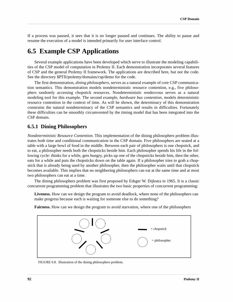
CSP Domain

If a process was paused, it sees that it is no longer paused and continues. The ability to pause andresume the execution of a model is intended primarily for user interface control.

6.5 Example CSP Applications

Several example applications have been developed which serve to illustrate the modeling capabili-ties of the CSP model of computation in Ptolemy II. Each demonstration incorporates several featuresof CSP and the general Ptolemy II framework. The applications are described here, but not the code.See the directory $PTII/ptolemy/domains/csp/demo for the code.

The first demonstration, dining philosophers, serves as a natural example of core CSP communica-tion semantics. This demonstration models nondeterministic resource contention, e.g., five philoso-phers randomly accessing chopstick resources. Nondeterministic rendezvous serves as a naturalmodeling tool for this example. The second example, hardware bus contention, models deterministicresource contention in the context of time. As will be shown, the determinacy of this demonstrationconstrains the natural nondeterminacy of the CSP semantics and results in difficulties. Fortunatelythese difficulties can be smoothly circumvented by the timing model that has been integrated into theCSP domain.

6.5.1 Dining Philosophers

Nondeterministic Resource Contention. This implementation of the dining philosophers problem illus-trates both time and conditional communication in the CSP domain. Five philosophers are seated at atable with a large bowl of food in the middle. Between each pair of philosophers is one chopstick, andto eat, a philosopher needs both the chopsticks beside him. Each philosopher spends his life in the fol-lowing cycle: thinks for a while, gets hungry, picks up one of the chopsticks beside him, then the other,eats for a while and puts the chopsticks down on the table again. If a philosopher tries to grab a chop-stick that is already being used by another philosopher, then the philosopher waits until that chopstickbecomes available. This implies that no neighboring philosophers can eat at the same time and at mosttwo philosophers can eat at a time.

The dining philosophers problem was first proposed by Edsger W. Dijkstra in 1965. It is a classicconcurrent programming problem that illustrates the two basic properties of concurrent programming:

Liveness. How can we design the program to avoid deadlock, where none of the philosophers can make progress because each is waiting for someone else to do something?

Fairness. How can we design the program to avoid starvation, where one of the philosophers

= chopstick

= philosopher

FIGURE 6.8. Illustration of the dining philosophers problem.

92 Ptolemy II

CSP Domain

could make progress but does not because others always go first?

This implementation uses an algorithm that lets each philosopher randomly chose which chopstick topick up first (via a CDO), and all philosophers eat and think at the same rates. Each philosopher andeach chopstick is represented by a separate process. Each chopstick has to be ready to be used by eitherphilosopher beside it at any time, hence the use of a CDO. After it is grabbed, it blocks waiting for amessage from the philosopher that is using it. After a philosopher grabs both the chopsticks next tohim, he eats for a random time. This is represented by calling delay() with the random interval to eatfor. The same approach is used when a philosopher is thinking. Note that because messages are passedby rendezvous, the blocking of a philosopher when it cannot obtain a chopstick is obtained for free.

This algorithm is fair, as any time a chopstick is not being used, and both philosophers try to use it,they both have an equal chance of succeeding. However, this algorithm does not guarantee the absenceof deadlock, and if it is let run long enough this will eventually occur. The probability that deadlockoccurs sooner increases as the thinking times are decreased relative to the eating times.

6.5.2 Hardware Bus Contention

Deterministic Resource Contention. This demonstration consists of a controller, N processors and amemory block, as shown in Figure 6.9. At randomly selected points in time, each processor requestspermission from the controller to access the memory block. The processors each have priorities associ-ated with them and in cases where there are simultaneous memory access requests, the controllergrants permission to the processor with the highest priority. Due to the atomic nature of rendezvous, itis impossible for the controller to check priorities of incoming requests while requests are occurring.To overcome this difficulty, an alarm is employed. The alarm is started by the controller immediatelyfollowing the first request for memory access at a given instant in time. It is awakened when a delayblock occurs to indicate to the controller that no more memory requests will occur at the given point intime. Hence, the alarm uses CSP’s notion of delay blocking to make deterministic an inherently non-deterministic activity.

6.6 Technical Details

6.6.1 Rendezvous Algorithm

In CSP, the locking point for all communication between processes is the receiver. Any time a pro-

FIGURE 6.9. Illustration of the Hardware Bus Contention example.

Processor ProcessorProcessor

Memory AlarmController


CSP Domain

cess wishes to send or receive, it must first acquire the lock for the receiver associated with its commu-nication channel. Two key facts to keep in mind when reading the following algorithms are that eachchannel has exactly one receiver associated with it and that at most one process can be trying to send to(or receive from) a channel at any stage. The constraint that each channel can have at most one processtrying to send to (or receive from) a channel at any stage is not currently enforced, but an exceptionwill be thrown if such a model is not constructed.

The rendezvous algorithm is entirely symmetric for the put() and the get(), except for the directionthe token is transferred. This helps reduce the number of deadlock situations that could arise and alsomakes the interaction between processes more understandable and easier to explain. The algorithm forget() is shown in figure 6.10. The algorithm for put() is exactly the same except that put and get areswapped everywhere. Thus it suffices to explain what happens when a get() arrives at a receiver, i.e.when a process tries to receive from the channel associated with the receiver.

When a get() arrives at a receiver, a put() is either already waiting to rendezvous or it is not. Boththe get() and put() methods are entirely synchronized on the receiver so they cannot happen simulta-neously (only one thread can possess a lock at any given time). Without loss of generality assume aget() arrives before a put(). The rendezvous mechanism is basically three steps: a get() arrives, a put()arrives, the rendezvous completes.

(1) When the get() arrives, it sees that it is first and sets a flag saying a get is waiting. It then waits on the receiver lock while the flag is still true,

(2) When a put() arrives, it sets the getWaiting flag to false, wakes up any threads waiting on the receiver (including the get), sets the rendezvousComplete flag to false and then waits on the receiver while the rendezvousComplete flag is false,

(3) The thread executing the get() wakes up, sees that a put() has arrived, sets the rendezvousCom-plete flag to true, wakes up any threads waiting on the receiver, and returns thus releasing the lock. The thread executing the put() then wakes up, acquires the receiver lock, sees that the rendezvous is complete and returns.

Following the rendezvous, the state of the receiver is exactly the same as before the rendezvousarrived, and it is ready to mediate another rendezvous. It is worth noting that the final step, of makingsure the second communication to arrive does not return until the rendezvous is complete, is necessaryto ensure that the correct token gets transferred. Consider the case again when a get() arrives first,except now the put() returns immediately if a get() is already waiting. A put() arrives, places a token inthe receiver, sets the getWaiting flag to false and returns. Now suppose another put() arrives before theget() wakes up, which will happen if the thread the put() is in wins the race to obtain the lock on thereceiver. Then the second put() places a new token in the receiver and sets the put waiting flag to true.Then the get() wakes up, and returns with the wrong token! This is known as a race condition, whichwill lead to unintended behavior in the model. This situation is avoided by our design.

6.6.2 Conditional Communication Algorithm

There are two steps involved in executing a CIF or a CDO: deciding which enabled branch suc-ceeds, and carrying out the rendezvous.

Built on top of rendezvous: When a conditional construct has more than one enabled branch (the guard is true or absent), a newthread is spawned for each enabled branch. The job of the chooseBranch() method is to control these

94 Ptolemy II

CSP Domain

threads and to determine which branch should be allowed to successfully rendezvous. These threadsand the mechanism controlling them are entirely separate from the rendezvous mechanism describedin section 6.6.1, with the exception of one special case, which is described in section 6.6.3. Thus theconditional mechanism can be viewed as being built on top of basic rendezvous: conditional communi-cation knows about and needs basic rendezvous, but the opposite is not true. Again this is a designdecision which leads to making the interaction between threads easier to understand and is less proneto deadlock as there are fewer interaction possibilities to consider.

get arrives

put waiting? get waiting = trueNo

notifyAll

_checkAndWaitget

waiting?

register actorblocked

register actorunblocked

rendezvouscomplete = true

notifyAll

No

Yes

put waiting = false

rendezvouscomplete = false

_checkAndWait

notifyAll

rendezvouscomplete?

No

Yes

Wakes upCondSend if oneis waiting

Yes

wakes up

wakes up

FIGURE 6.10. Rendezvous algorithm.


CSP Domain

Choosing which branch succeeds. The manner in which the choice of which branch can rendezvous is worth explaining. The choose-Branch() method in CSPActor takes an array of branches as an argument. If all of the guards are false,it returns -1, which indicates that all the branches failed. If exactly one of the guards is true, it performsthe rendezvous directly and returns the identification number of the successful branch. The interestingcase is when more than one guard is true. In this case, it creates and starts a new thread for each branchwhose guard is true. It then waits, on an internal lock, for one branch to succeed. At that point it getswoken up, sets a finished flag in the remaining branches and waits for them to fail. When all thethreads representing the branches are finished, it returns the identification number of the successfulbranch. This approach is designed to ensure that exactly one of the branches created performs a ren-dezvous successfully.

Algorithm used by each branch: Similar to the approach followed in rendezvous, the algorithm by which a thread representing a branchdetermines whether or not it can proceed is entirely symmetrical for a ConditionalSend and a Condi-tionalReceive. The algorithm followed by a ConditionalReceive is shown figure 6.12. Again the lock-ing point is the receiver, and all code concerned with the communication is synchronized on thereceiver. The receiver is also where all necessary flags are stored.

Consider three cases.

(1) A conditionalReceive arrives and a put is waiting.

In this case, the branch checks if it is the first branch to be ready to rendezvous, and if so, it is goes ahead and executes a get. If it is not the first, it waits on the receiver. When it wakes up, it checks if it is still alive. If it is not, it registers that it has failed and dies. If it is still alive, it starts again by trying to be the first branch to rendezvous. Note that a put cannot disappear.

(2) A conditionalReceive arrives and a conditionalSend is waiting

When both sides are conditional branches, it is up to the branch that arrives second to check whether the rendezvous can proceed. If both branches are the first to try to rendezvous, the condi-tionalReceive executes a get(), notifies its parent that it succeeded, issues a notifyAll() on the receiver and dies. If not, it checks whether it has been terminated by chooseBranch(). If it has, it registers with chooseBranch() that it has failed and dies. If it has not, it returns to the start of the algorithm and tries again. This is because a ConditionalSend could disappear. Note that the parent of the first branch to arrive at the receiver needs to be stored for the purpose of checking if both branches are the first to arrive.

This part of the algorithm is somewhat subtle. When the second conditional branch arrives at the

rendezvous

which branch should succeed?

FIGURE 6.11. Conceptual view of how conditional communication is built on top of rendezvous.

96 Ptolemy II

CSP Domain

rendezvous point it checks that both sides are the first to try to rendezvous for their respective pro-cesses. If so, then the conditionalReceive executes a get(), so that the conditionalSend is never aware that a conditionalReceive arrived: it only sees the get().

(3) A conditionalReceive arrives first.

It sets a flag in the receiver that it is waiting, then waits on the receiver. When it wakes up, it checks whether it has been killed by chooseBranch. If it has, it registers with chooseBranch that it has failed and dies. Otherwise it checks if a put is waiting. It only needs to check if a put is waiting because if a conditionalSend arrived, it would have behaved as in case (2) above. If a put is wait-ing, the branch checks if it is the first branch to be ready to rendezvous, and if so it is goes ahead

conditional receivearrives

put waiting? No

get!!branchSucceeded

Yes

conditionalsend waiting?

first branch torendezvous?

Yes

branchFailed No

Return

_checkAndWait

NoReturn

still alive?

a put cannotdissappear

Yesfirst branch torendezvous?

_checkAndWaitNo

a conditionalSendCAN dissappear

Yes

still alive?

Yes

other sidefirst branch torendezvous?

notifyAllNo

No

Yes

get!!branchSucceeded

Return

No

conditional receivewaiting = true

_checkAndWait

branchFailed No

Return

still alive?

Yes

put waiting?get!!

branchSucceededYes

Return

No

Yes

branchFailed No

Return

Case 1 Case 2Case 3

first branch torendezvous?

Yes

No

FIGURE 6.12. Algorithm used to determine if a conditional rendezvous branch succeeds or fails


CSP Domain

and executes a get. If it is not the first, it waits on the receiver and tries again.

6.6.3 Modification of Rendezvous Algorithm

Consider the case when a conditional send arrives before a get. If all the branches in the condi-tional communication that the conditional send is a part of are blocked, then the process will registeritself as blocked with the director. When the get comes along, and even though a conditional send iswaiting, it too would register itself as blocked. This leads to one too many processes being registeredas blocked, which could lead to premature deadlock detection.

To avoid this, it is necessary to modify the algorithm used for rendezvous slightly. The change tothe algorithm is shown in the dashed ellipse in figure 6.13. It does not affect the algorithm except in thecase when a conditional send is waiting when a get arrives at the receiver. In this case the process thatcalls the get should wait on the receiver until the conditional send waiting flag is false. If the condi-tional send succeeded, and hence executed a put, then the get waiting flag and the conditional sendwaiting flag should both be false and the actor proceeds through to the third step of the rendezvous. Ifthe conditional send failed, it will have reset the conditional send waiting flag and issued a notifyAll()on the receiver, thus waking up the get and allowing it to properly wait for a put.

The same reasoning also applies to the case when a conditional receive arrives at a receiver beforea put.

get waiting = true

notifyAll

_checkAndWaitget

waiting?

register actorblocked

register actorunblocked

No

Yes

_checkAndWaitconditionalsend waiting?

No

Yes

FIGURE 6.13. Modification of rendezvous algorithm, section 6.6.3, shown in ellipse.

98 Ptolemy II


7
DDE Domain
Author: John S. Davis II

7.1 Introduction

The distributed discrete-event (DDE) model of computation incorporates a distributed notion oftime into a dataflow style of computation. Time progresses in a DDE model when the actors in themodel execute and communicate. Actors in a DDE model communicate by sending messages throughbounded, FIFO channels. Time in a DDE model is distributed and localized, and the actors of a DDEmodel each maintain their own local notion of the current time. Local time information is sharedbetween two connected actors whenever a communication between said actors occurs. Conversely,communication between two connected actors can occur only when constraints on the relative localtime information of the actors are adhered to.

The DDE domain is based on distributed discrete-event processing and leverages a wealth ofresearch devoted to this topic. Some tutorial publications on this topic are [30][43][64][109]. The DDEdomain implements a specific variant of distributed discrete event systems (DDES) as expounded byChandy and Misra [30]. The domain serves as a framework for studying DDES with two specialemphases. First we consider DDES from a dataflow perspective; we view DDE as an implementationof the Kahn dataflow model [66] with distributed time added on top. Second we study DDES not withthe goal of improving execution speed (as has been the case traditionally). Instead we study DDES tolearn its usefulness in modeling and designing systems that are timed and distributed.

7.2 Using DDE

The DDE domain is typed so that actors used in a model must be derived from TypedAtomicActor.The DDE domain is designed to use both DDE specific actors as well as domain-polymorphic actors.DDE specific actors take advantage of DDEActor and DDEIOPort which are designed to provide con-venient support for specifying time when producing and consuming tokens. The DDE domain also hasspecial restrictions on how feedback is specified in models.

esign 99

DDE Domain

7.2.1 DDEActor

The DDE model of computation makes one very strong assumption about the execution of anactor: all input ports of an actor operating in a DDE model must be regularly polled to determinewhich input channel has the oldest pending event. Any actor that adheres to this assumption can oper-ate in a DDE model. Thus, many polymorphic actors found in ptolemy/actor/[lib, gui] are suitable foroperation in DDE models. For convenience, DDEActor was developed to simplify the construction ofactors that have DDE semantics. DDEActor has two key methods as follows:

getNextToken(). This method polls each input port of an actor and returns the (non-Null) token thatrepresents the oldest event. This method blocks accordingly as outlined in section 7.3.1 (Communicat-ing Time).

getLastPort(). This method returns the input IOPort from which the last (non-Null) token was con-sumed. This method presumes that getNextToken() is being used for token consumption.

7.2.2 DDEIOPort

DDEIOPort extends TypedIOPort with parameters for specifying time stamp values of tokens thatare being sent to neighboring actors. Since DDEIOPort extends TypedIOPort, use of DDEIOPorts willnot violate the type resolution protocol. DDEIOPort is not necessary to facilitate communicationbetween actors executing in a DDE model; standard TypedIOPorts are sufficient in most communica-tion. DDEIOPorts become useful when the time stamp to be associated with an outgoing token isgreater than the current time of the sending actor. Hence, DDEIOPorts are only useful in conjunctionwith delay actors (see “Enabling Communication: Advancing Time” on page 7-101, for a definition ofdelay actor). Most polymorphic actors available for Ptolemy II are not delay actors.

7.2.3 Feedback Topologies

In order to execute models with feedback cycles that will not deadlock, FeedBackDelay actorsmust be used. FeedBackDelay is found in the DDE kernel package. FeedBackDelay actors do not per-form computation, but instead increment the time stamps of tokens that flow through them by a speci-fied delay. The delay value of a FeedBackDelay actor must be chosen to be less than the delta time ofthe feedback cycle in which the FeedBackDelay actor is contained. Elaborate delay values can be spec-ified by overriding the getDelay() method in subclasses of FeedBackDelay. An example can be foundin ptolemy/domains/dde/demo/LocalZeno/ZenoDelay.java.

A difficulty found in feedback cycles occurs during the initialization of a model’s execution. Infigure 7.1 we see that even if Actor B is a FeedBackDelay actor, the system will deadlock if the firstevent is created by A since C will block on an event from B. To alleviate this problem a special timestamp value has been reserved: PrioritizedTimedQueue.IGNORE. When an actor encounters an eventwith a time stamp of IGNORE (an ignore event), the actor will ignore the event and the input channel

Actor A Actor C

Actor B

Actor D

FIGURE 7.1. Initializing feedback topologies.

100 Ptolemy II

DDE Domain

it is associated with. The actor then considers the other input channels in determining the next avail-able event. After a non-ignore event is encountered and consumed by the actor, all ignore events willbe cleared from the receivers. If all of an actor’s input channels contain ignore events, then the actorwill clear all ignore events and then proceed with normal operation.

The initialize method of FeedBackDelay produces an ignore event. Thus, in figure 7.1, if B is aFeedBackDelay actor, the ignore event it produces will be sent to C’s upper input channel allowing Cto consume the first event from A. The production of null tokens and feedback delays will then be suf-ficient to continue execution from that point on. Note that the production of an ignore event by a Feed-BackDelay actor serves as a major distinction between it and all other actors. If a delay is desiredsimply to represent the computational delay of a given model, a FeedBackDelay actor should not beused.

The intricate operation of ignore events requires special consideration when determining the posi-tion of a FeedBackDelay actor in a feedback cycle. A FeedBackDelay actor should be placed so thatthe ignore event it produces will be ignored in deference to the first real event that enters a feedbackcycle. Thus, choosing actor D as a FeedBackDelay actor in figure 7.1 would not be useful given thatthe first real event entering the cycle is created by A.

7.3 Properties of the DDE domain

Operationally, the semantics of the DDE domain can be separated into two functionalities. Thefirst functionality relates to how time advances during the communication of data and how communi-cation proceeds via blocking reads and writes. The second functionality considers how a DDE modelprevents deadlock due to local time dependencies. The technique for preventing deadlock involves thecommunication of null messages that consist solely of local time information.

7.3.1 Enabling Communication: Advancing Time

Communicating Tokens. A DDE model consists of a network of sequential actors that are connectedvia unidirectional, bounded, FIFO queues. Tokens are sent from a sending actor to a receiving actor byplacing a token in the appropriate queue where the token is stored until the receiving actor consumes it.As in the process networks domain, the execution of each actor is controlled by a process. If a processattempts to read a token from a queue that is empty, then the process will block until a token becomesavailable on the channel. If a process attempts to write a token to a queue that is full, then the processwill block until space becomes available for more tokens in that queue. Note that this blocking read/write paradigm is equivalent to the operational semantics found in non-timed process networks (PN) asimplemented in Ptolemy II (see the PN Domain chapter).

If all processes in a DDE model simultaneously block, then the model deadlocks. If a deadlock isdue to processes that are either waiting to read from an empty queue, read blocks, or waiting to write toa full queue, write blocks, then we say that the model has experienced non-timed deadlock. Non-timeddeadlock is equivalent to the notion of deadlock found in bounded process networks scheduling prob-lems as outlined by Parks [120]. If a non-timed deadlock is due to a model that consists solely of pro-cesses that are read blocked, then we say that a real deadlock has occurred and the model is terminated.If a non-timed deadlock is due to a model that consists of at least one process that is write blocked,then the capacity of the full queues are increased until deadlock no longer exists. Such deadlocks arecalled artificial deadlock, and the policy of increasing the capacity of full queues as shown by Parkscan guarantee the execution of a model in bounded memory whenever possible.


DDE Domain

Communicating Time. Each actor in a DDE model maintains a local notion of time. Any non-negativereal number may serve as a valid value of time. As tokens are communicated between actors, timestamps are associated with each token. Whenever an actor consumes a token, the actor’s current time isset to be equal to that of the consumed token’s time stamp. The time stamp value applied to outgoingtokens of an actor is equivalent to that actor’s output time. For actors that model a process in whichthere is delay between incoming time stamps and corresponding outgoing time stamps, then the outputtime is always greater than the current time; otherwise, the output time is equal to the current time. Werefer to actors of the former case as delay actors.

For a given queue containing time stamped tokens, the time stamp of the first token currently con-tained by the queue is referred to as the receiver time of the queue. If a queue is empty, its receiver timeis the value of the time stamp associated with the last token to flow through the queue, or 0.0 if notokens have traveled through the queue. An actor may consume a token from an input queue given thatthe queue has a token available and the receiver time of the queue is less than the receiver times of allother input queues of the actor. If the queue with the smallest receiver time is empty, then the actorblocks until this queue receives a token, at which time the actor considers the updated receiver time inselecting a queue to read from. The last time of a queue is the time stamp of the last token to be placedin the queue. If no tokens have been placed in the queue, then the last time is 0.0

Figure 7.2 shows three actors, each with three input queues. Actor A has two tokens available onthe top queue, no tokens available on the middle queue and one token available on the bottom queue.The receiver times of the top, middle and bottom queue are respectively, 17.0, 12.0 and 15.0. Since thequeue with the minimum receiver time (the middle queue) is empty, A blocks on this queue before itproceeds. In the case of actor B, the minimum receiver time belongs to the bottom queue. Thus, B pro-ceeds by consuming the token found on the bottom queue. After consuming this token, B compares allof its receiver times to determine which token it can consume next. Actor C is an example of an actorthat contains multiple input queues with identical receiver times. To accommodate this situation, eachactor assigns a unique priority to each input queue. An actor can consume a token from a queue if noother queue has a lower receiver time and if all queues that have an identical receiver time also have alower priority.

Each receiver has a completion time that is set during the initialization of a model. The completiontime of the receiver specifies the time after which the receiver will no longer operate. If the time stampof the oldest token in a receiver exceeds the completion time, then that receiver will become inactive.

7.3.2 Maintaining Communication: Null Tokens

Deadlocks can occur in a DDE model in a form that differs from the deadlocks described in theprevious section. This alternative form of deadlock occurs when an actor read blocks on an input porteven though it contains other ports with tokens. The topology of a DDE model can lead to deadlock asread blocked actors wait on each other for time stamped tokens that will never appear. Figure 7.3 illus-

Actor A

15.0

12.0

17.022.0

Actor B

15.0

22.0

17.022.0

Actor C

15.0

28.0

15.022.0

FIGURE 7.2. DDE actors and local time.

102 Ptolemy II

DDE Domain

trates this problem. In this topology, consider a situation in which actor A only creates tokens on itslower output queue. This will lead to tokens being created on actor C’s output queue but no tokens willbe created on B’s output queue (since B has no tokens to consume). This situation results in D readblocking indefinitely on its upper input queue even though it is clear that no tokens will ever flowthrough this queue. The result: timed deadlock! The situation shown in figure 7.3 is only one exampleof timed deadlock. In fact there are two types of timed deadlock: feedforward and feedback.

Figure 7.3 is an example of feedforward deadlock. Feedforward deadlock occurs when a set ofconnected actors are deadlocked such that all actors in the set are read blocked and at least one of theactors in the set is read blocked on an input queue that has a receiver time that is less than the localclock of the input queue’s source actor. In the example shown above, the upper input queue of B has areceiver time of 0.0 even though the local clock of A has advanced to 8.0.

Feedback deadlock occurs when a set of cyclically connected actors are deadlocked such that allactors in the set are read blocked and at least one actor in the set, say actor X, is read blocked on aninput queue that can read tokens which are directly or indirectly a result of output from that same actor(actor X). Figure 7.4 is an example of feedback timed deadlock. Note that B can not produce an outputbased on the consumption of the token timestamped at 5.0 because it must wait for a token on theupper input that depends on the output of B!

Preventing Feedforward Timed Deadlock. To address feedforward timed deadlock, null tokens areemployed. A null token provides an actor with a means of communicating time advancement eventhough data (real tokens) are not being transmitted. Whenever an actor consumes a token, it places anull token on each of its output queues such that the time stamp of the null token is equal to the currenttime of the actor. Thus, if actor A of figure 7.3, produced a token on its lower output queue at time 5.0,it would also produce a null token on its upper output queue at time 5.0.

If an actor encounters a null token on one of its input queues, then the actor does the following.First it consumes the tokens of all other input queues it contains given that the other input queues havereceiver times that are less than or equal to the time stamp of the null token. Next the actor removes thenull token from the input queue and sets its current time to equal the time stamp of the null token. Theactor then places null tokens time stamped to the current time on all output queues that have a last timethat is less then the actor’s current time. As an example, if B in figure 7.3 consumes a null token on itsinput with a time stamp of 5.0 then it would also produce a null token on its output with a time stamp

Actor D

Actor B

Actor C

Actor A Actor E

3.0 2.08.0 5.0

FIGURE 7.3. Timed deadlock (feedforward).

Actor CActor A Actor D

8.0 5.0

Actor B

FIGURE 7.4. Timed deadlock (feedback).


DDE Domain

of 5.0.The result of using null tokens is that time information is evenly propagated through a model’s

topology. The beauty of null tokens is that they inform actors of inactivity in other components of amodel without requiring centralized dissemination of this information. Given the use of null tokens,feedforward timed deadlock is prevented in the execution of DDE models. It is important to recognizethat null tokens are used solely for the purpose of avoiding deadlocks. Null tokens do not represent anyactual components of the physical system being modeled. Furthermore, the production of a null tokenthat is the direct result of the consumption of a null token is not considered computation from thestandpoint of the system being modeled. The idea of null tokens was first espoused by Chandy andMisra [30].

Preventing Feedback Timed Deadlock. We address feedback timed deadlock as follows. All feedbackloops are required to have a cumulative time stamp increment that is greater than zero. In other words,feedback loops are required to contain delay actors. Peacock, Wong and Manning [121] have shownthat a necessary condition for feedback timed deadlock is that a feedback loop must contain no delayactors. The delay value (delay = output time - current time) of a delay actor must be chosen wisely; itmust be less then the smallest delta time of all other actors contained in the same feedback loop. Deltatime is the difference between the time stamps of a token that is consumed by an actor and the corre-sponding token that is produced in direct response. If a system being modeled has characteristics thatprevent a fixed, positive lower bound on delta time from being specified, then our approach can notsolve feedback timed deadlock. Such a situation is referred to as a Zeno condition. An applicationinvolving an approximated Zeno condition is discussed in section 7.5 below.

The DDE software architecture provides one delay actor for use in preventing feedback timeddeadlock: FeedBackDelay. See “Feedback Topologies” on page 7-100 for further details about thisactor.

7.3.3 Alternative Distributed Discrete Event Methods

The field of distributed discrete event simulation, also referred to as parallel discrete event simula-tion (PDES), has been an active area of research since the late 1970’s [30][43][64][109][121].Recently there has been a resurgence of activity [8][9][16]. This is due in part to the wide availabilityof distributed frameworks for hosting simulations and the application of parallel simulation techniquesto non-research oriented domains. For example, several WWW search engines are based on network ofworkstation technology.

The field of distributed discrete event simulation can be cast into two camps that are distinguishedby the blocking read approach taken by the actors. One camp was introduced by Chandy and Misra[30][43][109][121] and is known as conservative blocking. The second camp was introduced by DavidJefferson through the Jet Propulsion Laboratory Time Warp system and is referred to as the optimisticapproach [64][43]. In certain problems, the optimistic approach executes faster than the conservativeapproach, nevertheless, the gains in speed result in significant increases in program memory. The con-servative approach does not perform faster than the optimistic approach but it executes efficiently forall classes of discrete event systems. Given the modeling semantics emphasis of Ptolemy II, perfor-mance (speed) is not considered a premium. Furthermore, Ptolemy II’s embedded systems emphasissuggests that memory constraints are likely to be strict. For these reasons, the implementation found inthe DDE domain follows the conservative approach.

104 Ptolemy II

DDE Domain

7.4 The DDE Software Architecture

For a model to have DDE semantics, it must have a DDEDirector controlling it. This ensures thatthe receivers in the ports are DDEReceivers. Each actor in a DDE model is under the control of aDDEThread. DDEThreads contain a TimeKeeper that manages the local notion of time that is associ-ated with the DDEThread’s actor.

7.4.1 Local Time Management

The UML diagram of the local time management system of the DDE domain is shown in figure7.5 and consists of PrioritizedTimedQueue, DDEReceiver, DDEThread and TimeKeeper. Since time islocalized, the DDEDirector does not have a direct role in this process. Note that DDEReceiver isderived from PrioritizedTimedQueue. The primary purpose of PrioritizedTimedQueue is to keep trackof a receiver’s local time information. DDEReceiver adds blocking read/write functionality to Priori-tizedTimedQueue.

FIGURE 7.5. Key classes for managing time locally.

DDEThread

+DDEThread(actor : Actor, director : ProcessDirector)+getTimeKeeper() : TimeKeeper+noticeOfTermination()+start()+wrapup()

ProcessThread

«Interface»ProcessReceiver

AtomicActor

1..1

1..1 controls

1..1

1..1

manages time for

1..1

1..1

IOPort

0..n

0..1contains

0..n

1..1 containsDDEReceiver

+DDEReceiver()+DDEReceiver(cntr : IOPort)+DDEReceiver(cntr : IOPort, priority : int)+hasToken(branch : Branch) : boolean+prepareToBlock(branch : Branch)+put(token : Token)+put(token : Token, time : double, branch : Branch)+wakeUpBlockedPartner()#_hideNullTokens(hide : boolean)

-_terminate : boolean-_hideNullTokens : boolean

PrioritizedTimedQueue

+PrioritizedTimedQueue()+PrioritizedTimedQueue(p : IOPort)+PrioritizedTimedQueue(p : IOPort, priority : int)+getCapacity() : int+getLastTime() : double+getReceiverTime() : double+hasRoom() : boolean+hasRoom(numberOfTokens : int) : boolean+hasToken() : boolean+hasToken(numberOfTokens : int) : boolean+put(token : Token, time : double)+removeIgnoredToken() : void+reset() : void+setCapacity(capacity : int)#_getCompletionTime() : double#_hasNullToken() : boolean#_setCompletionTime(t : double)#_setReceiverTime(time : double)

+ETERNITY : double+IGNORE : double+INACTIVE : double#_lastTime : double#_priority : int-_completionTime : double-_receiverTime : double

TimeKeeper

+TimeKeeper(actor : Actor) : void+getCurrentTime() : double+getFirstReceiver() : PrioritizedTimedQueue+getNextTime() : double+getOutputTime() : double+removeAllIgnoredTokens() : void+sendOutNullTokens(receiver : DDEReceiver) : void+setCurrentTime(time : double) : void+updateReceiverList(queue : PrioritizedTimedQueue) : void#_setOutputTime(time : double) : void#_setReceiverPriorities() : void

-_currentTime : double-_outputTime : double

ReceiverComparator

+ReceiverComparator(keeper : TimeKeeper)+compare(first : Object, second : Object) : int

0..n

contains

«Interface»Comparator

AbstractReceiver


DDE Domain

When a DDEDirector is initialized, it instantiates a DDEThread for each actor that the directormanages. DDEThread is derived from ProcessThread. The ProcessThread class provides functionalitythat is common to all of the process domains (e.g., CSP, DDE and PN). The directors of all processdomains (including DDE) assign a single actor to each ProcessThread. ProcessThreads take responsi-bility of their assigned actor’s execution by invoking the iteration methods of the actor. The iterationmethods are prefire(), fire() and postfire(); ProcessThreads also invoke wrapup() on the actors theycontrol.

DDEThread extends the functionality of ProcessThread. Upon instantiation, a DDEThread createsa TimeKeeper object and assigns this object to the actor that it controls. The TimeKeeper gets access toeach of the DDEReceivers that the actor contains. Each of the receivers can access the TimeKeeperand through the TimeKeeper the receivers can then determine their relative receiver times. With thisinformation, the receivers are fully equipped to apply the appropriate blocking rules as they get and puttime stamped tokens.

DDEReceivers use a dynamic approach to accessing the DDEThread and TimeKeeper. To ensuredomain polymorphism, actors (DDE or otherwise) do not have static references to the TimeKeeper andDDEThread that they are controlled by. To ensure simplified mutability support, DDEReceivers do nothave a static reference to TimeKeepers. Access to the local time management facilities is accom-plished via the Java Thread.currentThread() method. Using this method, a DDEReceiver dynamicallyaccesses the thread responsible for invoking it. Presumably the calling thread is a DDEThread andappropriate steps are taken if it is not. Once the DDEThread is accessed, the corresponding Time-Keeper can be accessed as well. The DDE domain uses this approach extensively in DDERe-ceiver.put(Token) and DDEReceiver.get().

7.4.2 Detecting Deadlock

The other kernel classes of the DDE domain are shown in figure 7.6. The purpose of the DDEDi-rector is to detect and (if possible) resolve timed and/or non-timed deadlock of the model it controls.Whenever a receiver blocks, it informs the director. The director keeps track of the number of activeprocesses, and the number of processes that are either blocked on a read or write. Artificial deadlocksare resolved by increasing the queue capacity of write-blocked receivers.

Note the distinction between internal and external read blocks in DDEDirector’s package friendlymethods. The current release of DDE assumes that actors that execute according to a DDE model ofcomputation are atomic rather than composite. In a future Ptolemy II release, composite actors will befacilitated in the DDE domain. At that time, it will be important to distinguish internal and externalread blocks. Until then, only internal read blocks are in use.

7.4.3 Ending Execution

Execution of a model ends if either an unresolvable deadlock occurs, the director’s completiontime is exceeded by all of the actors it manages, or early termination is requested (e.g., by a user inter-face button). The director’s completion time is set via the public stopTime parameter of DDEDirector.The completion time is passed on to each DDEReceiver. If a receiver’s receiver time exceeds the com-pletion time, then the receiver becomes inactive. If all receivers of an actor become inactive and theactor is not a source actor, then the actor will end execution and its wrapup() method will be called. Insuch a scenario, the actor is said to have terminated normally.

Early terminations and unresolvable deadlocks share a common mechanism for ending execution.Each DDEReceiver has a boolean _terminate flag. If the flag is set to true, then the receiver will

106 Ptolemy II

DDE Domain

throw a TerminateProcessException the next time any of its methods are invoked. TerminatePro-cessExceptions are part of the ptolemy/actor/process package and ProcessThreads know to endan actor’s execution if this exception is caught. In the case of unresolvable deadlock, the _terminateflag of all blocked receivers is set to true. The receivers are then awakened from blocking and theyeach throw the exception.

7.5 Example DDE Applications

To illustrate distributed discrete event execution, we have developed an applet that features a feed-back topology and incorporates polymorphic as well as DDE specific actors. The model, shown in fig-ure 7.7, consists of a single source actor (ptolemy/actor/lib/Clock) and an upper and lower branch offour actors each. The upper and lower branches have identical topologies and are fed an identicalstream of tokens from the Clock source with the exception that in the lower branch ZenoDelayreplaces FeedBackDelay.

As with all feedback topologies in DDE (and DE) models, a positive time delay is necessary infeedback loops to prevent deadlock. If the time delay of a given loop is lower bounded by zero but cannot be guaranteed to be greater than a fixed positive value, then a Zeno condition can occur in whichtime will not advance beyond a certain point even though the actors of the feedback loop continue toexecute without deadlocking. ZenoDelay extends FeedBackDelay and is designed so that a Zeno con-dition will be encountered. When execution of the model begins, both FeedBackDelay and ZenoDelay

FIGURE 7.6. Additional classes in the DDE kernel.

DDEDirector

+DDEDirector()+DDEDirector(workspace : Workspace)+DDEDirector(container : CompositeEntity, name : String)+hasMutation() : boolean#_actorBlocked(receiver : DDEReceiver)#_actorBlocked(receivers : LinkedList)#_actorUnblocked(receivers : LinkedList)#_actorUnBlocked(receiver : DDEReceiver)#_getInitialTimeTable() : Hashtable#_incrementLowestCapacityPort()#_resolveInternalDeadlock() : boolean

+stopTime : Parameter

DDEActor

+DDEActor()+DDEActor(workspace : Workspace)+DDEActor(container : CompositeEntity, name : String)+getLastPort() : TypedIOPort+getNextToken() : Token#_getNextInput() : Token

-_currentTime : double-_lastPort : TypedIOPort

DDEIOPort

+DDEIOPort()+DDEIOPort(container : ComponentEntity, name : String)+DDEIOPort(container : ComponentEntity, name : String, in : boolean, out : boolean)+broadcast(token : Token, sendTime : double)+send(channel : int, token : Token, sendTime : double)+setContainer(container : ComponentEntity)

TypedIOPortCompositeProcessDirector

FeedBackDelay

+FeedBackDelay()+FeedBackDelay(workspace : Workspace)+FeedBackDelay(container : CompositeEntity, name : String)+getDelay() : double+setDelay(delay : double)

+input : TypedIOPort+nullDelay : Parameter+output : TypedIOPort+realDelay : Parameter#_delay : double

NullToken

Token

TypedAtomicActor


DDE Domain

are used to feed back null tokens into Wire so that the model does not deadlock. After local timeexceeds a preset value, ZenoDelay reduces its delay so that the lower branch approximates a Zeno con-dition.

In centralized discrete event systems, Zeno conditions prevent progress in the entire model. This istrue because the feedback cycle experiencing the Zeno condition prevents time from advancing in theentire model. In contrast, distributed discrete event systems localize Zeno conditions as much as ispossible based on the topology of the system. Thus, a Zeno condition can exist in the lower branch andthe upper branch will continue its execution unimpeded. Localizing Zeno conditions can be useful inlarge scale modeling in which a Zeno condition may not be discovered until a great deal of time hasbeen invested in execution of the model. In such situations, partial data collection may proceed prior tocorrection of the delay error that resulted in the Zeno condition.

Lower Branch

DoubleFork

Clock

TimedWire

FeedBackDelay

Plotter

DoubleFork PlotterWire

ZenoDelay

Timed

Upper Branch

FIGURE 7.7. Localized Zeno condition topology.

108 Ptolemy II

Heterogeneous Concurrent Modeling and

8
PN Domain
Author: Mudit GoelContributors: Adam Cataldo

Steve Neuendorffer

8.1 Introduction

The process networks (PN) domain in Ptolemy II models a system as a network of processes thatcommunicate with each other by passing messages through unidirectional first-in-first-out (FIFO)channels. A process blocks when trying to read from an empty channel until a message becomes avail-able on it. This model of computation is deterministic in the sense that the sequence of values commu-nicated on the channels is completely determined by the model. Consequently, a process network canbe evaluated using a completely parallel schedule, a completely sequential schedule, or any schedulein between, always yielding the same output results for a given input sequence.

PN is a natural model for describing signal processing systems where infinite streams of data sam-ples are incrementally transformed by a collection of processes executing in parallel. Embedded signalprocessing systems are good examples of such systems. They are typically designed to operate indefi-nitely with limited resources. This behavior is naturally described as a process network that runs for-ever but with bounded buffering on the communication channels whenever possible.1

PN can also be used to model concurrency in the various hardware components of an embeddedsystem. The process networks model of computation can model the functional behavior of these sys-tems and test them for their functional correctness, but it cannot directly model their real-time behav-ior. To address the involvement of time, we have extended the PN model such that it can include thenotion of time.

Some systems might display adaptive behavior like migrating code, agents, and arrivals and depar-tures of processes. To support this adaptive behavior, we provide a mutation mechanism that supports

1. In general, bounded buffers cannot be ensured for an arbitrary process network. An important part of the design of a process network concerns showing that the buffers are, in fact, bounded. Synchronous dataflow models are an important type of process network which always have bounded buffers.

Design 109

PN Domain

addition, deletion, and changing of processes and channels. With untimed PN, this might display non-determinism, while with timed-PN, it becomes deterministic.

The PN model of computation is a superset of the synchronous dataflow model of computation(see the SDF Domain chapter). Consequently, any SDF actor can be used within the PN domain. How-ever, the execution of the model is very different from SDF, since a separate process is created for eachactor. These processes are implemented as Java threads [116].

8.2 Using PN

There are two issues we consider in the PN domain:• Deadlock in feedback loops• Designing actors

8.2.1 Deadlock in Feedback Loops

Feedback loops in PN are handled in much the same way as in the SDF domain. One of the actorsin the feedback loop must create a number of tokens in its feedback loop in order to break the datadependency. Just like in the SDF domain, the SampleDelay actor can be used for this purpose.Remember, however, that the PN domain does not (and cannot) statically analyze the model to deter-mine the size of the delay necessary in the feedback loop. It is up to the designer of the model to spec-ify the correct amount of delay.

8.2.2 Designing Actors

In our PN domain implementation, it is not possible for an actor to check if data is present at aninput port. The hasToken() method always returns true indicating that a token is present, and if a tokenis not actually present, then the get() method will block until one becomes available. This allows mod-els to execute deterministically. However, actors that take inputs from more than one input can oftenbe difficult to write. An example is the Select actor; a control input is read first, and the data from thatport determines which input port to read from.

8.3 Properties of the PN domain

Two important properties of the PN domain implemented in Ptolemy II are that processes commu-nicate asynchronously (by ordered queues) and that the memory used in the communication isbounded whenever possible. The PN domain in Ptolemy II can be used with or without a notion oftime.

8.3.1 Asynchronous Communication

In [65][66], Kahn and MacQueen describe a model of computation where processes are connectedby communication channels to form a network. Processes produce data elements or tokens and sendthem along a unidirectional communication channel where they are stored in a FIFO queue until thedestination process consumes them. This is a form of asynchronous communication between pro-cesses. Communication channels are the only method processes may use to exchange information. Aset of processes that communicate through a network of FIFO queues defines a program.

110 Ptolemy II

PN Domain

Kahn and MacQueen require that execution of a process be suspended when it attempts to get datafrom an empty input channel (blocking reads). Hence, a process may not poll a channel for presence orabsence of data. At any given point, a process is either doing some computation (enabled) or it isblocked waiting for data (read blocked) on exactly one of its input channels; it cannot wait for datafrom more than one channel simultaneously. Systems that obey this model are determinate; the historyof tokens produced on the communication channels does not depend on the execution order. Therefore,the results produced by executing a program are not affected by the scheduling of the various pro-cesses.

In case all the processes in a model are blocked while trying to read from some channel, then wehave a real deadlock; none of the processes can proceed. Real deadlock is a program state that happensirrespective of the schedule chosen for the processes in a model. This characteristic is guaranteed bythe determinacy property of process networks.

8.3.2 Bounded Memory Execution

The high level of concurrency in process networks makes it an ideal match for embedded systemsoftware and for modeling hardware implementations. A characteristic of these embedded applicationsand hardware processes, is that they are intended to run indefinitely with a limited amount of memory.One problem with directly implementing the Kahn-MacQueen semantics is that bounded memory exe-cution of a process network is not guaranteed, even if it is possible. Hence, bounded memory executionof process networks becomes crucial for its usefulness for hardware and embedded software.

In [120], Parks addresses this aspect of process networks and provides an algorithm to make a pro-cess network application execute in bounded memory whenever possible. He provides an implementa-tion of the Kahn-MacQueen semantics using blocking writes that assigns a fixed capacity to each FIFOchannel and forces processes to block temporarily if a channel is full. Thus a process now has threestates: running (executing), read blocked, or write blocked and a process may not poll a channel foreither data or room.

In addition to the real deadlock described above, the introduction of a blocking write operation cancause an artificial deadlock of the process network. In this situation, all the processes in a model areblocked and at least one process is blocked on a write. However, unlike a real deadlock, a program cancontinue after artificial deadlock by increasing the capacity of the channels on which processes arewrite blocked. In particular, Parks chooses to increase only the capacity of the channel with the small-est capacity among the channels on which processes are write blocked. This algorithm minimizes over-all required memory in the channels and is used in the PN domain to handled artificial deadlock.

8.3.3 Time

In real-time systems and embedded applications, the real time behavior of a system is as importantas the functional correctness. Process networks can be used to describe the functional properties of asystem, but cannot describe temporal properties since the basic model lacks the notion of time. Onesolution is to use some other timed model of computation, such as DE, for describing temporal proper-ties. Another solution is to extend the process networks model of computation with a notion of time, aswe have done in Ptolemy II. This extension is based on the Pamela model [46], which was originallydeveloped for modeling the performance of parallel systems using Dykstra’s semaphores.

In the timed PN domain, time is global. All processes in a model share the same time, which isreferred to as the current time or model time. A process can explicitly wait for time to advance, bydelaying itself for some fixed amount of time. After being suspended for the specified amount of time,


PN Domain

the process wakes up and continues to execute. If the process delays itself for zero time then the pro-cess simply continues to execute.

In the timed PN domain, time changes only at specific moments and never during the execution ofa process. The time observed by a process can only advance when it is in one of the following twostates:

1. The process is delayed and is explicitly waiting for time to advance (delay block).

2. The process is waiting for data to arrive on one of its input channels (read block).When all the processes in a program are in one of these two states, then the program is in a state of

timed deadlock. The fact that at least one process is delayed, distinguishes timed deadlock from otherdeadlocks. When timed deadlock is detected, the current time is advanced until at least one process canwake up from a delay block and the model continues executing.

8.3.4 Mutations

The PN domain tolerates mutations, which are run-time changes in the model structure. Normally,mutations are realized as change requests queued with the model. In PN there is no determinate pointwhere mutations can occur other than a real deadlock. However, being able to perform mutations atthis point is unlikely as a real deadlock might never occur. For example, a model with even one non-terminating source never experiences a real deadlock. Therefore mutations cannot be performed atdeterminate points since the processes in the network are not synchronized. Executing mutations atarbitrary times introduces non-determinism in PN, since the state of the processes is unknown.

In timed PN, however, the presence of timed deadlock provides a regular point at which the stateof execution can be determined. This means that mutations in timed PN can be made deterministically.Implementation details are presented in the next section.

8.4 The PN Software Architecture

The PN domain kernel is realized in the package ptolemy.domains.pn.kernel. The structure dia-gram of the package is shown in figure 8.1.

8.4.1 PNDirector

This class extends the CompositeProcessDirector base class to add Kahn process networks (PN)semantics. This director does not support mutations or a notion of time. It provides only a mechanismto perform blocking reads and writes using bounded memory execution whenever possible.

This director is capable of handling both real and artificial deadlocks. Artificial deadlock isresolved as soon as it arises using Parks’ algorithm as explained in section 8.3.2. Real deadlock, how-ever, cannot be handled locally and must rely on the external environment to provide more data forexecution to continue.

PNDirector has a parameter called initialQueueCapacity that sets the initial capacities of thequeues in all the receivers created in the PN domain. Another parameter, maximumQueueCapacity,sets the upper bound on the queue capacities.

8.4.2 TimedPNDirector

TimedPNDirector extends the PNDirector to introduce a notion of global time to the model. It also

112 Ptolemy II

PN Domain

provides for deterministic execution of mutations. Mutations are performed at the earliest timed-dead-lock that occurs after they are queued. Since occurrence of timed-deadlock is deterministic, perform-ing mutations at this point makes mutations deterministic. The TimedPNDirector is currentlyexperimental; there are not very many tests for it.

8.4.3 PNQueueReceiver

The PNQueueReceiver implements the ProcessReceiver interface and contains a FIFO queue torepresent a process network communication channel. These receivers are also responsible for imple-menting the blocking reads and blocking writes through the get() and put() methods.

When the get() method is called, the receiver first checks whether its FIFO queue has any token. Ifnot, it reports to the director that the reading thread is blocked waiting for data. It also sets an internalflag to indicate that a thread is read blocked. Then the reading thread is suspended until some otherthread puts a token into the FIFO queue. At this point, the flag of the receiver is reset to false, thedirector is notified that a process has unblocked, the reading process retrieves the first token from theFIFO queue and execution continues.

The put() method of the receiver works similarly by first checking whether the FIFO queue is atfull capacity. If so, it reports to the director that the writing thread is blocked waiting for space in thequeue. It also sets an internal flag to indicate that a thread is write blocked. The writing thread blocksuntil some other thread gets a token from the FIFO queue, or the size of the queue is increased by thedirector because the model reached an artificial deadlock. In either case, the director is notified that awriting process unblocks and the internal flag is reset. The writing thread wakes up and its token is

PNDirector

+PNDirector()+PNDirector(workspace : Workspace)+PNDirector(container : CompositeEntity, name : String)+addProcessListener(listener : PNProcessListener)+removeProcessListener(listener : PNProcessListener)

+initialQueueCapacity : Parameter+maximumQueueCapacity : Parameter

«Interface»Receiver

PNQueueReceiver

+PNQueueReceiver()+PNQueueReceiver(container : IOPort)+prepareToBlock(branch : Branch)+setReadPending(readPending : boolean)+setWritePending(writePending : boolean)+wakeUpBlockedPartner()

QueueReceiver

FIFOQueue

1..1

1..1

TimedPNDirector

+TimedPNDirector()+TimedPNDirector(workspace : Workspace)+TimedPNDirector(container : CompositeEntity, name : String)+fireAt(actor : Actor, newFiringTime : double)+setCurrentTime(newTime : double)

«Interface»ProcessReceiver

CompositeProcessDirector

FIGURE 8.1. Static structure of the PN kernel.


PN Domain

placed into the receiver.

8.4.4 Handling Deadlock

Every time an actor in PN blocks, the count of blocked actors is incremented. If the total number ofactors blocked or paused by user request equals the total number of actors active in the simulation, adeadlock is detected. On detection of a deadlock, if one or more actors are blocked on a write, then thisis an artificial deadlock. The channel with the smallest capacity among all the channels with actorsblocked on a write is chosen and its capacity is doubled. This implements the bounded memory execu-tion of [120]. If a real deadlock is detected, then the fire() method of the director returns, allowing acontaining model to present more data to the inputs of the process network.

8.4.5 Finite Iterations

An important aspect of Ptolemy II is that the firing of an actor, or an entire model is guaranteed tocomplete. In the PN domain the end of a firing occurs when deadlock is reached. The deadlock can bereal or timed deadlock. However, in a process network real deadlock may never actually happen. Inthis case, in order to manually stop execution or to execute mutations there needs to be a way to halt allthe executing threads in the network. This is handled by the stopFire() method of the executable inter-face. The PN director implements this method to set a flag in each process which causes the process topause. Note that as with most domains, it is not possible to simply call the wrapup() method of the pro-cess director, since the fire method has not yet returned.

8.4.6 NondeterministicMerge

The PN domain supports a NondeterministicMerge actor, which merges two incoming streamsnondeterministically. This actor should be used with caution, since determinism is one of the key fea-tures of PN. Use of this actor is risky because any given execution is only representative of the possibleexecutions. Nonetheless, this offers a considerable increment in expressiveness.

114 Ptolemy II


9
PSDF Domain
Author: Steve NeuendorfferContributor: Shuvra Bhattacharyya

9.1 Purpose of the Domain

The parameterized synchronous dataflow (PSDF) domain is useful for modeling dataflow systemswith reconfiguration. Reconfiguration allows more interesting systems to be modeled without resort tomore generalized dataflow models. As such, the PSDF domain represents a design point between com-plete static scheduling in the synchronous dataflow (SDF) domain, and completely dynamic executionunder the process networks (PN) domain. Under the PSDF domain, symbolic analysis of the model isused to generate a quasi-static schedule that statically determines an execution order of actors, butdynamically determines the number of times each actor fires. The quasi-static schedule guaranteesbounded memory execution as long as the parameters that the schedule depends on are bounded. Addi-tionally, the model is guaranteed to be deadlock free, regardless of the parameter values. The primarydisadvantage of the PSDF domain is that current scheduling techniques are only valid for acyclicgraphs.

9.2 Using PSDF

There are several issues that must be addressed when using the PSDF domain, in addition to thenormal issues of synchronous dataflow models:• Restricted reconfiguration• Symbolic scheduling limitations

This section will present a short description of these issues. For a more complete description, seesection 9.3.

gn 115

PSDF Domain

9.2.1 Restricted Reconfiguration

Consider the SDF model shown in figure 9.1. This model displays arrays of various sizes. Everytime the SequenceToArray actor fires, it consumes an integer indicating the size of the next array fromthe Ramp actor and then consumes that many tokens from its top input port and wraps them into anarray. The SequenceToArray actor in this case is obviously not valid in SDF, since its rates change.This particular model is also not a valid PSDF model, although with some modifications it can bemade valid.

The difficulty with the below model arises because the schedule for the model depends on the run-time value consumed from the Ramp actor. However, this value is not consumed (or even produced)until after the schedule has begun executing. In the terminology of parameterized synchronous data-flow, the model is not locally synchronous[15]. One solution is to build the model hierarchically, asshown in figure 9.2. In this model, the Ramp actor executes first, and reconfigures the PSDF model.The reconfiguration happens before the PSDF schedule begins executing, and the quasi-static scheduleis instantiated with the correct token rates. Another possible solution would be to make the model aprocess network instead, but this would preclude static scheduling and efficient code generation.

FIGURE 9.1. A PSDF model that is not locally synchronous.

FIGURE 9.2. The model of figure 9.1 corrected using hierarchy.

116 Ptolemy II

PSDF Domain

9.2.2 Symbolic scheduling limitations

Parameterized synchronous dataflow scheduling results in a quasi-static schedule. In contrast tosynchronous dataflow schedules, which are a simple sequence of actor firings, a quasi-static scheduleis more of a program that generates a sequence at runtime. Essentially, the goal of the PSDF scheduleris to find a fixed program that will generate the correct schedules for any parameter value. PSDFscheduling for models without feedback is reasonably understood. Additionally, in models where feed-back does not restrict scheduling, the feedback can be eliminated for parameterized scheduling. How-ever, for models with tight feedback loops, scheduling is not quite as simple and the feedback cannotbe eliminated. The current scheduler implementation provides none of these improvements and onlyschedules models without feedback.

Another limitation of symbolic scheduling is that it must rely on a general symbolic math packageto guarantee a valid schedule. One solution is to provide side information to the model, to assist withsymbolic simplification. The current scheduler implementation provides no mechanism for this.

9.3 Properties of the PSDF domain

PSDF is an untimed model of computation, similar to the SDF domain (see Chapter 3). The keyimprovement is that the PSDF domain generates a schedule by considering the token consumption andproduction rates symbolically. Data rates on each port are allowed to change through reconfiguration,as long as reconfiguration does not occur during execution of the schedule, implying that the model islocally synchronous. Reconfiguration analysis is performed to statically determine when rate parame-ters change to ensure a valid schedule.

9.3.1 Scheduling

The first step in constructing synchronous dataflow schedules is to solve the balance equations[87]. These equations determine the number of times each actor will fire during an iteration. Ordi-narily, these equations are solved for a numeric solution, and an equivalent schedule is generated. Inthe PSDF domain, the balance equations are solved for a symbolic solution in the other variables. Thesymbolic solutions are converted into a quasi-static schedule where the number of firings of each actoris computed at run-time. For example, consider the model in figure 9.3. This model implies the follow-ing system of equations, where ProductionRate and ConsumptionRate are declared properties of eachport, and Firings is a property of each actor that will be solved for:

Firings(A) × ProductionRate(A1) = Firings(B) × ConsumptionRate(B1)

E0

D1: SDF director

A1

AA2

C1C

C2

B1

BB2

FIGURE 9.3. An example SDF model.


PSDF Domain

Firings(A) × ProductionRate(A2) = Firings(C) × ConsumptionRate(C1)

Firings(C) × ProductionRate(C2) = Firings(B) × ConsumptionRate(B2)

These equations express constraints that the number of tokens created on a relation during an iterationis equal to the number of tokens consumed. A symbolic solution to these equations asserts, forinstance, that:

Firings(A) = ConsumptionRate(B1) / (gcd(ConsumptionRate(C1) * ProductionRate(A1) / gcd(Pro-ductionRate(A2), ConsumptionRate(C1)), ConsumptionRate(B1))) * ConsumptionRate(C1) / gcd(Pro-

ductionRate(A2), ConsumptionRate(C1))

where gcd(a,b) is the greatest common divisor of a and b. As with SDF models, it is possible for amodel to be inconsistent, where no symbolic solution to the balance equations exists.

The second step in constructing a PSDF schedule is dataflow analysis. Dataflow analysis in anordinary synchronous dataflow model orders the firing of actors, based on the relations between them.In SDF scheduling, dataflow analysis involves simulation of the schedule execution until each actorhas been fired the required number of times. In PSDF scheduling, the situation is more complex, sincethe number of times an actor will fire is not known beforehand. To simplify the problem, we assumethat each actor appears exactly once in the schedule, and executes the number of times according to thesymbolic balance equations. This simplification cannot be done for all models with feedback, but canalways be done for models without feedback, hence the restriction mentioned in the previous section.

9.3.2 Local Synchrony and Reconfiguration Analysis

Although rate parameters in PSDF models are allowed to change between schedule iterations, theymust not change during the execution of a schedule. This property is known as local synchrony. Inorder to ensure local synchrony of PSDF models, reconfiguration analysis is performed during sched-uling. This reconfiguration analysis combines information on parameter dependency (which parame-ters depend on other parameters) and reconfiguration (which models modify parameter values). Theresult of reconfiguration analysis is the least change context of a parameter. The least change contextof a parameter is a composite actor that contains the parameter, reconfigures the parameter, and is con-tained by all other composite actors that reconfigure the parameter. Local synchrony requires that rateparameters used for scheduling are either not reconfigured, or have a least change context that containsthe PSDF model or is the PSDF model.

Reconfiguration analysis considers the following possible types of reconfiguration:Reconfiguration ports: PortParameters are reconfigured when tokens are received from a Parame-

terPort.Modal Models: Parameters may be reconfigured in finite-state machine transitions.Reconfiguration analysis is performed in a similar matter to data type analysis. A set of inequali-

ties are extracted from a model where each inequality represents a constraint on the least change con-text of a parameter. One class of constraint requires that the least change context of a parameter Pcannot be any higher in the hierarchy than the least change context of a parameter that P depends on.The second constraint requires that if a parameter is reconfigured by an actor, then the actor must con-tain the least change context of the parameter. These constraints are solved to determine the leastchange context of every parameter. The PSDF scheduler uses this information to check for local syn-chrony of the model and to reduce symbolic computations where possible if some rate parameters arenot reconfigured. The algorithm is described more completely in [102].

118 Ptolemy II

PSDF Domain


The PSDF kernel package implements the PSDF model of computation. The structure of this pack-age is similar to the structure of the SDF kernel package. The PSDF scheduler relies on a schedulinglibrary built by students at the University of Maryland. This library implements a parameterized ver-sion of the APGAN algorithm and makes relatively few optimizations to the symbolic schedule.Unlike the SDF domain, the PSDF domain computes external port rates which may be symbolic. TheSDF domain also leverages reconfiguration analysis to detect such cases and report a modeling error.

Reconfiguration analysis is implemented by the ptolemy.actor.util.ConstVariableModelAnalysisclass. This analysis operates globally on a model and is intended to be used during the preinitializationphase of execution by schedulers. The ConstVariableModelAnalysis class relies on declarations byobjects in a model which directly invoke the setToken() method on other parameters during executionof a model. The ptolemy.domains.fsm.FSMActor class and the ptolemy.actor.parameters.Parameter-Port class implement the ptolemy.actor.util.ExplicitChangeContext interface to declare that they mod-ify parameters directly. On some occasions, an object might detect a changed parameter, such asthrough the attributeChanged() method and modify another parameter. Such objects are expected touse the ptolemy.actor.util.DependencyDeclaration attribute to declare this parameter dependence,which would otherwise not be visible to the reconfiguration analysis. Dependencies which arisethrough parameter expressions are directly understood by the reconfiguration analysis and do not needto be explicitly declared.

9.5 Actors

Most domain-polymorphic actors can be used under the PSDF domain, with similar restrictions aswith the SDF domain. The SampleDelay actor can be used in PSDF models, although models withfeedback are not.


PSDF Domain

120 Ptolemy II


10
HDF Domain
Author: Ye Zhou

10.1 Introduction

The heterochronous dataflow (HDF) domain is useful for modeling dataflow systems withrestricted flow controls. Under the synchronous dataflow (SDF) domain (see Chapter 3), the set of portrates (called rate signatures) of an actor are constant, and the schedule is statically determined prior toexecution. The HDF domain extends the SDF domain by allowing changes in rate signatures betweeniterations. Within each iteration, rate signatures are fixed and an HDF model behaves like an SDFmodel. This guarantees that a schedule can be completely executed. Between iterations, the HDFdomain checks if there is any rate change and recomputes the schedule when necessary.

10.2 Using HDF in Vergil

The HDF domain is often used with a modal model, whose local director is configured to anHDFFSMDirector. The change of rate signatures is modeled by state transitions of the modal model, inwhich each state refinement infers a set of rate signatures. The HDFFSMDirector restricts that statetransitions can only occur between global iterations.

Figure 10.1 shows an HDF model example. The toplevel uses an HDF director. The modal modelis constructed in the same way as discussed in section 4.4. To configure the modal model with anHDFFSMDirector as its local director, double click on the modal model. Set the directorClass param-eter to ptolemy.domains.hdf.kernel.HDFFSMDirector.

10.2.1 Data Rates of the Modal Model

The HDF domain uses the hierarchical scheduling algorithm of SDF to schedule modal models.The port rates of a modal model in HDF are the external port rates of its current state refinement. Astate refinement could be an SDF model, or another HDF model. A state may also refine to anotherdomain that doesn’t have the notion of port rates. In this case, the default values of the rate parameters

gn 121

HDF Domain

are used. For more details on port rate parameters, see section 3.4.2.Note that a state in the modal model of HDF is restricted to have exactly one refinement, in order

to define a unique set of rate signatures of the modal model. There is only one exception. A state mayhave no refinement if upon being entered, it has an outgoing transition with a guard expression that istrue. This will be treated as a transient state1. Transient states can have preemptive and non-preemp-tive transitions, while non-transient states are assumed to have only non-preemptive transitions. Whena modal model reaches a transient state, it will progress through that state to the next state until itencounters a state with a refinement. An exception is thrown if the mode controller (FSMActor)reaches a transient state but cannot get out of it.

10.2.2 Multi-Token Syntax in Guard Expressions

A modal model with an HDFFSMDirector as its local director may consume and produce multipletokens on each firing. Therefore, we develop a syntax to address multiple tokens in guard expressions.This is implemented by creating an additional input variable2 for each port (or channel if the port is amultiport) in the FSMActor. If the port is a single port, an array value variable named portNameArrayis used. If the port is a multiport, an array value variable named portName_channelIndexArray is usedfor each channel. An array value variable is an array of variables that have the same type as the corre-sponding input. For an FSMActor governed by an HDFFSMDirector, the array value variable containsall the token received from the input in one iteration. We use portNameArray(i) orportName_channelIndexArray(i) to indicate the (i+1)-th most recent token received from that port(channel). The state variable portName_isPresent (or portName_channelIndex_isPresent) is true ifthere is at least one token at the corresponding port (or channel), and otherwise false. The value vari-able portName (or portName_channelIndex) is by default the last (most recent) token received. I.e.,portName = portNameArray(0).

In the following example, we assume that a modal model has a single input port input, which con-sumes three tokens in one iteration.• Guard expression: inputArray(0) + inputArray(1) > 10. If the last two tokens received

from the input port have a sum greater than 10, the transition is enabled. Note that if there are

1. Here the notion of transient state is different from what is defined in hybrid systems.2. The introduction of input variables of an FSMActor can be found in section 4.3.1.

FIGURE 10.1. An HDF model example.

A B

M

HDF Director


SDF Director SDF Director

HDFFSM Director

A B

M

HDF Director


SDF Director SDF Director

HDFFSM Director

122 Ptolemy II

HDF Domain

fewer than two tokens in the array value variable when the expression is evaluated, an exceptionwill be thrown.

• Guard expression: input + inputArray(1) > 10. This has the same meaning as the aboveexample.

• Guard expression: input_isPresent && input > 0. If at least one token is received from theinput port and the last token has a value greater than 0, the transition is enabled.

Guard expressions for multiport can be written in similar ways.

10.2.3 Actions in Modal Model

Set actions can be used in modal model to set parameters of the FSMActor. However, outputAc-tions should not be used in HDF since any output produced by the FSMActor will introduce conflictswith the port rates declared by the state refinement. The outputs of the modal model in HDF are allproduced by the state refinement.

10.3 Properties of the HDF domain

The HDF domain inherits most of the SDF properties. The notion of iteration and vectorizationalso apply to HDF.

10.3.1 Scheduling

The scheduling of HDF follows the hierarchical scheduling algorithm in SDF. Within each itera-tion, a modal model appears to be no different from the outside than an atomic actor, whose port ratesare set by the current state refinement. Since HDF uses modal models to define different sets of ratesignatures, it has only a finite number of schedules. We use a cache to save all these schedules, sowhen a state is revisited, we do not need to recompute the schedule again. The size of the cache is setby the scheduleCacheSize parameter of the HDF director.

10.3.2 Hierarchical Heterogeneous Models

An HDF model itself is a heterogeneous composition of dataflow models with FSM. An HDFmodel can generally be embedded in any other domain, with similar restrictions as with the SDFdomain.


The HDF kernel package includes an HDFDirector class and an HDFFSMDirector class.

10.4.1 HDF Director

The HDFDirector class extends the SDFDirector class by caching the schedules and dynamicallyobtain schedules between iterations. When an HDF director is created, it is automatically associatedwith an instance of the default scheduler class, CachedSDFScheduler, which is in the SDF kernel pack-age. The CachedSDFScheduler extends the SDFScheduler class by maintaining a cache of schedules.It is very efficient if only a moderate number of SDF schedules are used alternatively during execution.


HDF Domain

When the HDF model visits a new state (and hence a new set of rate signatures) in the modal model,the CachedSDFScheduler computes the schedule and saved it in the cache labeled with the corre-sponding rate signatures. Next time when this state is revisited, the HDF director obtains the schedulefrom the cache by identifying the rate signatures.

The cache also maintains an order of the schedules, with the most recently used schedule at thehead of the cache. If the cache is full, the least recently used schedule is discarded. The size of thecache is set by the scheduleCacheSize parameter of the HDF director, which takes an integer. If theparameter is set to a non-positive integer, it indicates the cache does not have a size limit. The defaultvalue of the parameter is 100.

The receivers in an HDF model are instances of SDFReceiver, in order to read and write tokens ina first-in-first-out (FIFO) order as in SDF.

10.4.2 HDFFSM Director

An HDFFSM director collaborates with an HDF director and governs the execution of a modalmodel in HDF. The HDFFSMDirector class extends the MultirateFSMDirector class in the FSM ker-nel package. The MultirateFSM director extends the FSM director by supporting the consumption andproduction of multiple tokens on a port in a firing. The HDFFSMDirector class further extends theMultirateFSMDirector by restricting that state transitions can only occur between global iterations.This is implemented by calling its requestChange() method, which is used to queue topology changes(mutations). Mutations are only executed between global iterations. Therefore, state transitions in HDFhappen less often than basic finite state machines, where transitions can occur between firings.

The receivers of a modal model with a MultirateFSM or HDFFSM director as its local director areinstances of SDFReceiver. Inputs to the FSMActor inside the modal model are read in a FIFO order.

10.5 Actors

Most domain-polymorphic actors can be used under the HDF domain, with similar restrictions aswith the SDF domain. The SampleDelay actor can be used in HDF models. However, SampleDelayactors inside state refinements might be problematic. One reason is that hiding initial tokens insideopaque composite actors may cause deadlock. On the other hand, the notion of initial tokens in theguard expressions are not supported.

124 Ptolemy II

Heterogeneous Concurrent Modeling and Des

11
DDF Domain
Author: Gang Zhou

11.1 Introduction

The dynamic dataflow (DDF) domain is a superset of the synchronous dataflow (SDF) and Bool-ean dataflow (BDF) domains. (BDF domain is not implemented in Ptolemy II yet, but available inPtolemy Classic.) In the SDF domain, an actor consumes and produces a fixed number of tokens perfiring. This static information makes possible compile-time scheduling. In the BDF domain, the staticanalysis techniques used in SDF are extended to allow Boolean-controlled dataflow actors and in somecases a quasi-static schedule can be pre-computed where each firing is annotated with the run-timeconditions under which the firing should occur. In the DDF domain, there are few constraints on theproduction and consumption behavior of actors, and the schedulers make no attempt to construct acompile-time schedule. Instead, each actor has a set of firing rules (patterns) and can be fired if one ofthem is satisfied, i.e., one particular firing pattern forms a prefix of sequences of unconsumed tokens atinput ports.

While the DDF domain can be used to model the most general form of dataflow systems, it is aspecial case of Kahn process networks. Instead of using the blocking read semantics of Kahn processnetworks, dataflow actors use firing rules for specifying conditions for invocations, each of whichdefines a quantum of computation. Using this quantum avoids the complexities and context switchingoverhead of process suspension and resumption incurred in most implementations of Kahn processnetworks. Instead of context switching, dataflow systems are executed by scheduling the actor firings.

Most of the contents of this chapter is based on [147]. Interested readers should refer to it for moredetails.

11.2 Properties of the DDF domain

To understand how the DDF domain works, one must first understand the firing rules for a generaldynamic dataflow actor. Then one must also understand the criteria a particular dynamic scheduling

ign 125

DDF Domain

algorithm is designed for.

11.2.1 Firing Rules

A general dynamic dataflow actor with m inputs and n outputs is defined by a pair {f, R} satisfyingthe following conditions3:• f: is a firing function where is a set of m-tuple sequences,• is a set of finite sequences called the firing rules,• is finite for all ,• no two distinct are joinable, i.e., they are not the prefixes of the same sequence.

When a firing rule forms a prefix of the sequence of unconsumed tokens at inputs, the actor is saidto be enabled and a firing can be invoked by consuming tokens in the firing rule and producing tokensresulting from applying the firing function f. Note that actors with no inputs (i.e., sources) are alwaysenabled.

The dynamic dataflow actors that can be used in the current DDF domain must also satisfy sequen-tial firing rules. Intuitively, sequential means that the firing rules can be tested in a pre-defined orderusing only blocking reads. Readers can refer to [85] for its technical definition. Some concrete exam-ples are provided in section 11.3.2 on writing DDF actors.

11.2.2 Scheduling

Given a DDF graph, there can be numerous ways to schedule its execution. The simplest way onecan think of is to keep firing any arbitrary enabled actor until either the graph is deadlocked or somepredefined stop condition is reached. However, there are many problems with this naïve scheduler. Forone, the execution may need unbounded memory whereas some other scheduler may only needbounded memory. Therefore we need some criteria to determine whether some scheduler is a “good”scheduler. It is important to point out that there are no absolute criteria. Different people can pose dif-ferent criteria as long as they can interpret their choice in a reasonable way.

The criteria used here were first realized in Ptolemy Classic, where the first criterion has higherpriority over the second one, the second one over the third one and so on:

1. After any finite time the token sequence (including consumed tokens) on any channel is a prefix ofthe least fixed-point given by the denotational semantics. (Correctness)

2. The scheduler should be able to execute a graph forever if it is possible to execute a graph forever.In particular, it should not stop prematurely if there are enabled actors. (Liveness)

3. The scheduler should be able to execute a graph forever in bounded memory if it is possible to exe-cute the graph forever in bounded memory. (Boundedness)

4. The scheduler should execute the graph in a sequence of well-defined and determinate iterations sothat the user can control the length of an execution by specifying the number of iterations to exe-cute. (Determinacy4)If a schedule satisfies condition 1, it is called a correct execution. To get a correct execution, we

3. A generalization of this is left out for the purpose of clearness. Interested readers should refer to [79].4. Here the notion of determinacy is different from that used in describing the intrinsic behavior of a model itself,

i.e., the determinacy of the channel history.

Sm

Sn→ S

m

R Sm⊆

f r( ) r R∈

r r' R∈,

126 Ptolemy II

DDF Domain

require that the operational semantics of a graph defined by a scheduler be consistent with its denota-tional semantics.

If a schedule satisfies condition 2 and 3, it is called a useful execution. In particular, condition 2requires that for every non-terminating model, after any finite time, the execution will extend at leastone sequence on some channel in additional finite time. Note the subtlety here. It does not require toextend every sequence. Condition 3 is for the purpose of practical implementation. Among all possibleschedulers, we would prefer those that can execute the graph with bounded memory. As pointed out byParks [120], liveness is a property of the model itself (directly related with lengths of sequences in itsdenotational semantics), whereas boundedness is a property of both the model and its scheduler. Buckproved in his Ph.D. thesis [22] that a BDF graph is Turing-complete. Since the BDF domain is a subsetof the DDF domain, a DDF graph is also Turing-complete. This has the consequence that both livenessand boundedness are undecidable for DDF graphs, meaning that no finite analysis can answer thequestion about these properties for any arbitrary DDF model. However, since a DDF scheduler hasinfinite time to run an infinite execution, there may exist schedulers that can satisfy both conditions, asParks’ algorithm did for Process Networks.

Condition 4 expresses the desire to extend the concept of iterations in the SDF domain to DDFdomain. In SDF, one iteration is defined as the minimum (but non-empty) complete cycle throughwhich the graph returns to its original state (defined as the number of tokens in each channel). This canbe determined by doing static analysis on the SDF graph. Then an SDF graph can be executed byrepeating iterations, and the user can control the length of execution by specifying the number of itera-tions in one execution. In DDF, there is no such inherent iteration. But we still want to define a some-what meaningful iteration which achieves something such as printing a dot on a plotter (whichinvolves invoking that actor once). And the set of actors executed in each iteration is determinate sothat the state of the model is a well-defined function of the number of iterations. This requires thatwhich actors to fire in each iteration should not depend on arbitrary decisions made by the scheduler,like the order in which it examines the enabling status of each actor. This way the user can control theprogress of the model using the similar mechanism as in SDF.

The particular scheduler implemented in the DDF domain is based on a scheduler in Ptolemy Clas-sic. The pseudo-code of the scheduling algorithm is given in figure 11.1. The intuition behind thisscheduler is that we defer firing of each enabled actor until it is absolutely necessary in order to avoiddeadlock. Thus we don’t create more tokens than necessary on each channel. To capture this notion, adeferrable actor is defined as one with any output channel (except a self-loop) that already has enoughtokens to satisfy the demand of the destination actor. There are a few subtle points here. First, if theactor has multiple output channels, it only takes one output channel satisfying one destination actorconnected to that channel to be a deferrable actor. Second, when one particular channel of a destinationactor is satisfied, it has two possible situations. One situation is that the number of tokens buffered onthat channel is greater than or equal to the number of tokens required for the next firing of the destina-tion actor. Another situation is that the destination actor does not consume a token on that channel dur-ing the next firing. Third, when one particular channel of a destination actor is satisfied, it does notmean the destination actor is enabled. It may be still waiting for tokens on different channels to enablethe next firing. The consequence is that we cannot use the prefire() method of the destination actor tocheck the deferability. Each actor must expose the number of tokens consumed on each input channelas part of its interface, which may dynamically change from one firing to another.


DDF Domain

11.3 Software Architecture and Implementation

The DDF domain kernel is realized in the package ptolemy.domains.ddf.kernel. The packageincludes an ActorEnablingStatus class and a DDFDirector class.

The ActorEnablingStatus class is a type-safe enumeration of three statuses an active actor may bein during the execution: ENABLED_DEFERRABLE, ENABLED_NOT_DEFERRABLE andNOT_ENABLED.

Since the communication style in a dataflow network is asynchronous message passing, we need afirst-in-first-out queue to act as the receiver in the DDF domain. There are two kinds of receivers thatare already implemented in the software which can be used for this purpose. One is the SDFReceiver,which contains an ArrayFIFOQueue implemented with a circular array. Another is the QueueReceiverwhich contains a FIFOQueue implemented with a LinkedList. The latter is used for the DDF domain.

11.3.1 DDFDirector

DDFDirector directly extends Director class. It implements a model of computation according tothe DDF semantics and a particular dynamic scheduling algorithm outlined in figure 11.1. The meth-ods that define the execution phases of the DDFDirector are implemented as follows:• initialize(): classify all actors into three categories: actors that are not enabled, actors that are

enabled but deferrable, and actors that are enabled and not deferrable. Search actors for a parame-ter named requiredFiringsPerIteration, which specifies the number of times the correspondingactor must be fired in one iteration.

• prefire(): check the input ports of the container composite actor (if necessary) to see whether

FIGURE 11.1. The pseudo-code of the scheduling algorithm implemented in the DDF domain.

At the start of each basic iteration compute {

E = set of enabled actors

D = set of deferrable and enabled actors

minimax(D) = subset of D as defined below

}

One basic (default) iteration consists of {

If (E \ D != Ø)

fire (E \ D)

else if (D != Ø)

fire minimax(D)

else

declare deadlock

}

minimax(D) = subset of D with the smallest maximum number of tokenson their output channels which satisfy the demands ofdestination actors

128 Ptolemy II

DDF Domain

they have enough tokens for the next iteration. Reset to zero the counting variables for those actorswhich are required to fire specified number of times in each iteration.

• fire(): perform one iteration of the model, which by default is one basic iteration. However, ifsome actor has a parameter named requiredFiringsPerIteration, continue to execute basic itera-tions until the actor has been fired at least the number of times given by that parameter. If morethan one actor has such a parameter, then the iteration will continue until all are satisfied. If theparameter runUntilDeadlockInOneIteration of the director has value true, one single iteration con-sists of repeating the basic iteration until deadlock is reached (thus overriding the previous defini-tion of one iteration), which is the status of the model where all active actors under the control ofthis director are unable to fire because their firing rules are not satisfied. However, they may beable to fire again during next iteration when tokens are transferred in from an outside domain.After each actor is fired, immediately determine the new status of the actors directly connected tothis actor as well as itself since the rest of the actors won’t be affected.

• postfire(): returns false when the value specified in the director parameter iterations has beenreached (there is no upper limit if the parameter is left with its default value 0) or the model comesto a deadlock in the current iteration.

Besides the two parameters runUntilDeadlockInOneIteration and iterations mentioned above,DDFDirector has a third parameter maximumReceiverCapacity, which sets the upper bound on thereceiver capacities. Its default value 0 means no upper limit.

The DDF domain tolerates mutations, which are run-time changes in the model structure. Nor-mally, mutations are realized as change requests queued with the model. The requests are executedbetween iterations of top level model and any new actors are initialized and become active for the nextiteration. Some high-order components can also perform mutations by themselves, such as ActorRe-cursion which can be used to design models with recursion at the actor-oriented level.

11.3.2 Writing DDF Actors

In SDF, the scheduling algorithm relies on the actors in the model to declare the data rate of eachport with up to three parameters named tokenConsumptionRate, tokenProductionRate, and tokenInit-Production. The production parameters are valid only for output ports, while the consumption parame-ter is valid only for input ports. If a valid parameter is not specified when the scheduler runs, thendefault values of the parameters corresponding to a homogeneous actor will be assumed: input portsare assumed to have a consumption rate of one, output ports are assumed to have a production rate ofone, and no tokens produced during initialization. If there are multiple channels connected to a multi-port, all channels are assumed to have the same rate given by the parameter.

In DDF, the director also relies on the tokenConsumptionRate parameter of each input port todetermine whether an actor is enabled/deferrable. However, unlike an SDF actor, the dynamic natureof a DDF actor dictates that this parameter will have a possible new value after each firing and thusmust be updated if needed. The tokenProductionRate parameter has no use in DDF because for a gen-eral DDF actor this information is not available before the actor gets fired. The tokenInitProductionparameter serves the same purpose as in SDF.

The BooleanSelect actor is a canonical actor in DDF domain and its design is representative ofDDF actors. In the DDF domain, it is renamed DDFBooleanSelect to distinguish it from BooleanSe-lect used in other domains such as DE. The actor has two firing rules. The first rule says if the controlport has a true token, the trueInput port must have a token and the second rule says if the control porthas a false token, the falseInput port must have a token. Compared with SDF actor firing rule which


DDF Domain

only specifies the number of tokens each input port must consume, the firing rules of DDFBooleanSe-lect actor also assert the token values of some input port. It seems that just providing the rate informa-tion wouldn’t be enough to distinguish between different firing rules. However, it turns out that for alarge category of actors which use so-called sequential firing rules, we can decompose an originalactor firing into multiple firings and in each of new firings, the rate information would be enough todetermine if an actor is enabled. This is because sequential means that the firing rules can be tested ina pre-defined order using only blocking reads. Each blocking read can be expressed as rate informationon the corresponding input port. Upon consuming the token, the actor determines the next input port toread token from, and the corresponding rate information is updated to reflect that.

The firing rules of DDFBooleanSelect actor are sequential, therefore we can introduce a two-phasefirings for this actor. During initialization, the control port sets its rate to 1 and trueInput/falseInputports both set their rates to 0. Figure 11.2 shows the code block for the initialization.

In the first firing, the actor consumes a Boolean token from control port. Depending on the Bool-ean value of that token (true or false), the corresponding port (trueInput or falseInput) changes its rateto 1 and the other port keeps its rate at 0. The control port also needs to change its rate to 0 to declarethat it doesn’t consume token in the next firing. In the second firing, trueInput port or falseInput portwith rate 1 consumes one token and sends it to the output port. Then the actor resets the rate parame-ters of all input ports the same as before the first firing. Figure 11.3 shows the code block for the split-phase firing. Figure 11.4 shows the code block for the rate update after each firing.

Another extension to the SDF domain involves rate declaration for multiports, which allow multi-ple-channel connections. In SDF, all channels connected to the same multiport have the same rate. This

FIGURE 11.2. Initialization code of DDFBooleanSelect actor.

public void initialize() throws IllegalActionException {super.initialize();_isControlRead = false;trueInput_tokenConsumptionRate.setToken(_zero);falseInput_tokenConsumptionRate.setToken(_zero);control_tokenConsumptionRate.setToken(_one);

}

private boolean _control;private boolean _isControlRead;private final static IntToken _zero = new IntToken(0);private final static IntToken _one = new IntToken(1);

FIGURE 11.3. Split-phase firing code of DDFBooleanSelect actor.

public void fire() throws IllegalActionException {super.fire();if (_isControlRead) {

if (_control) {output.send(0, trueInput.get(0));

} else {output.send(0, falseInput.get(0));

}_isControlRead = false;

} else {_control = ((BooleanToken) control.get(0)).booleanValue();_isControlRead = true;

}}

130 Ptolemy II

DDF Domain

won’t work for some dynamic actors. For example, the DDFSelect actor is very similar to DDFBool-eanSelect actor functionally. Its input port is a multiport because the actor communicates via an inde-terminate number of channels depending on the connections made to the input port. The control portconsumes an integer token, and its value specifies the input channel that should be read in the next fir-ing. In this case, an ArrayToken is used to represent the rates of the channels connected to the multi-port. The length of the array is equal to the width of the port, i.e., the number of channels connected tothe port. Each element of the array represents the rate of a channel in the order channels are createdwhile building the model. Figure 11.5 shows the code block for the initialization of all ArrayTokensand their exemplary uses for the DDFSelect actor.

It is interesting to notice that two actors BooleanSwitch and Switch, the counterparts of Bool-eanSelect and Select, don’t need special treatment to be used in DDF domain. They only have one fir-ing rule, i.e., each input channel needs one token. And that’s the default firing rule if no rate parametersare declared.

Finally, all SDF actors can be directly used in the DDF domain since the SDF domain is a subset ofthe DDF domain.

11.4 Example DDF Applications

This section gives several examples to show how conditionals, data-dependent iterations andrecursions can be modeled in the DDF domain.

11.4.1 Conditionals with If-Else Structure

The DDF-inside-SDF example in figure 11.6 demonstrates an if-then-else like structure in thedataflow context. In this example, the DDF composite actor looks like an SDF actor from outside. ArequiredFiringsPerIteration parameter is added to the DDFBooleanSelect actor and its value is set to2. In each iteration of the DDF composite actor, each input port consumes one token. Depending on theBoolean value of the token consumed from the control input port, the token consumed from the rampinput port is routed to the upper or the lower branch. Then it is processed by some actor and the resultemerges from DDFBooleanSelect actor. Finally it is transferred to the outside through the output port.

FIGURE 11.4. Rate update code of DDFBooleanSelect actor.

public boolean postfire() throws IllegalActionException {if (_isControlRead) {

if (_control) {trueInput_tokenConsumptionRate.setToken(_one);falseInput_tokenConsumptionRate.setToken(_zero);control_tokenConsumptionRate.setToken(_zero);

} else {trueInput_tokenConsumptionRate.setToken(_zero);falseInput_tokenConsumptionRate.setToken(_one);control_tokenConsumptionRate.setToken(_zero);

}} else {

trueInput_tokenConsumptionRate.setToken(_zero);falseInput_tokenConsumptionRate.setToken(_zero);control_tokenConsumptionRate.setToken(_one);

}return super.postfire();

}


DDF Domain

11.4.2 Data-Dependent Iterations

The model in figure 11.7 illustrates a do-while like structure in the dataflow context. Each numberproduced by Ramp actor is repeatedly multiplied by 0.5 until the product is below 0.5. The outside-the-loop Plotter has a requiredFiringsPerIteration parameter with value 1. Therefore each iteration in thismodel corresponds to a complete do-while loop for each number produced by Ramp actor.

FIGURE 11.5. Initialization of ArrayTokens and their exemplary uses for the DDFSelect actor.

public void connectionsChanged(Port port) {super.connectionsChanged(port);if (port == input) {

_rateArray = new ArrayToken[input.getWidth()];Token[] rate = new IntToken[input.getWidth()];for (int i = 0; i < input.getWidth(); i++) {

rate[i] = _zero;}try {

_rateZero = new ArrayToken(rate);for (int i = 0; i < input.getWidth(); i++) {

rate[i] = _one;_rateArray[i] = new ArrayToken(rate);rate[i] = _zero;

}} catch (IllegalActionException ex) {

// shouldn't happenthrow new InternalErrorException(ex);

}}

} public boolean postfire() throws IllegalActionException {

if (_isControlRead) {input_tokenConsumptionRate.setToken(_rateArray[_control]);control_tokenConsumptionRate.setToken(_zero);

} else {input_tokenConsumptionRate.setToken(_rateZero);control_tokenConsumptionRate.setToken(_one);

}return super.postfire();

}

private int _control;private boolean _isControlRead;private final static IntToken _one = new IntToken(1);private final static IntToken _zero = new IntToken(0);

/** An array of ArrayTokens to be used to set tokenConsumptionRate * of the input port. Each ArrayToken indicates the <i>input</i> * port needs to consume one token from a corresponding channel and * no token from the rest of the channels. The array is initialized * in the method connectionsChanged(). */private ArrayToken[] _rateArray;

/** An ArrayToken to be used to set tokenConsumptionRate of the input * port. It indicates the <i>input</i> port does not consume any token * from any channel. This variable is initialized in the method * connectionsChanged(). */private ArrayToken _rateZero;

132 Ptolemy II

DDF Domain

FIGURE 11.6. A model illustrating if-then-else structure.

FIGURE 11.7. A model illustrating do-while structure.


DDF Domain

11.4.3 Recursion

Eratosthenes (276 - 196 B.C.) invented a method called Sieve of Eratosthenes for efficiently con-structing tables of prime numbers. The method goes like this: first, write down a list of increasing inte-gers beginning with 2. Then filter out all multiples of 2. Move to the next remaining number, which inthis case is 3, then filter out all its multiples. Continue in this fashion and filter out all multiples of thenext remaining number. The numbers that are left up to the current remaining number are all primenumbers. In principle, this process can be repeated indefinitely to find any prime number.

It is interesting to see it implemented in a dataflow context in figure 11.8. The focus is on ActorRe-cursion, which is a composite actor with a StringParameter named recursionActor. Upon firing, itclones the composite actor containing itself and referred to by recursionActor. It places the cloneinside itself and connects the corresponding ports of both actors. In this example, recursionActor refersto Prime_Number_Filter. Therefore upon firing, ActorRecursion clones a filter inside itself to filter outthe multiples of the current remaining number and thus exactly implements the algorithm of Sieve ofEratosthenes.

FIGURE 11.8. A model illustrating recursion structure for computing prime numbers.

134 Ptolemy II

References

[1] G. Agha, Actors: A Model of Concurrent Computation in Distributed Systems, MIT Press, Cam-bridge, MA, 1986.

[2] G. Agha, “Abstracting Interaction Patterns: A Programming Paradigm for Open Distributed Sys-tems,” in Formal Methods for Open Object-based Distributed Systems, IFIP Transactions, E.Najm and J.-B. Stefani, Eds., Chapman & Hall, 1997.

[3] G. Agha, “Concurrent object-oriented programming,” Communications of the ACM, 33(9):125–140, Sept. 1990.

[4] G. Agha, S. Frolund, W. Kim, R. Panwar, A. Patterson, and D. Sturman, “Abstraction and modu-larity mechanisms for concurrent computing. IEEE Parallel and Distributed Technology: Systemsand Applications, 1(2):3–14, May 1993.

[5] G. Agha, I. A. Mason, S. F.Smith, and C. L. Talcott, “A foundation for actor computation. Journalof Functional Programming, 7(1):1–72, 1997.

[6] R. Allen and D. Garlan, “Formalizing Architectural Connection,” in Proc. of the 16th Interna-tional Conference on Software Engineering (ICSE 94), May 1994, pp. 71-80, IEEE ComputerSociety Press.

[7] G. R. Andrews, Concurrent Programming — Principles and Practice, Addison-Wesley, 1991.

[8] R. L. Bagrodia, “Parallel Languages for Discrete Event Simulation Models,” IEEE Computa-tional Science & Engineering, vol. 5, no. 2, April-June 1998, pp 27-38.

[9] R. Bagrodia, R. Meyer, et al., “Parsec: A Parallel Simulation Environment for Complex Sys-tems,” IEEE Computer, vol. 31, no. 10, October 1998, pp 77-85.

[10] P. Baldwin, S. Kohli, E. A. Lee, X. Liu and Y. Zhao, “Modeling of Sensor Nets in Ptolemy II,” InProceedings of Information Processing in Sensor Networks (IPSN), Berkeley, CA, USA, April26-27, 2004.

[11] P. Baldwin, S. Kohli, E. A. Lee, X. Liu and Y. Zhao, “Visualsense: Visual Modeling for Wirelessand Sensor Network Systems,” Technical Memorandum UCB/ERL M04/08, University of Cali-fornia, Berkeley, April 23, 2004.

[12] M. von der Beeck, “A Comparison of Statecharts Variants,” in Proc. of Formal Techniques inReal Time and Fault Tolerant Systems, LNCS 863, pp. 128-148, Springer-Verlag, 1994.

[13] A. Benveniste and G. Berry, “The Synchronous Approach to Reactive and Real-Time Systems,”Proceedings of the IEEE, Vol. 79, No. 9, 1991, pp. 1270-1282.

[14] A. Benveniste and P. Le Guernic, “Hybrid Dynamical Systems Theory and the SIGNAL Lan-guage,” IEEE Tr. on Automatic Control, Vol. 35, No. 5, pp. 525-546, May 1990.


[15] G. Berry and G. Gonthier, “The Esterel synchronous programming language: Design, semantics,implementation,” Science of Computer Programming, 19(2):87-152, 1992.

[16] S. Bhatt, R. M. Fujimoto, A. Ogielski, and K. Perumalla, “Parallel Simulation Techniques forLarge-Scale Networks,” IEEE Communications Magazine, Vol. 36, No. 8, August 1998, pp. 42-47.

[17] S. S. Bhattacharyya, P. K. Murthy and E. A. Lee, Software Synthesis from Dataflow Graphs, Klu-wer Academic Publishers, Norwell, Mass, 1996.

[18] J. Bier, E. Goei, W. Ho, P. Lapsley, M. O'Reilly, G. Sih and E. A. Lee, “Gabriel: A Design Envi-ronment for DSP,” IEEE Micro Magazine, October 1990, vol. 10, no. 5, pp. 28-45.

[19] C. H. Brooks and E. A. Lee, “Ptolemy II Coding Style,” Technical Memorandum UCB/ERLM03/44, University of California at Berkeley, November 24, 2003.

[20] Randy Brown, “CalendarQueue: A Fast Priority Queue Implementation for The Simulation EventSet Problem”, Communications of the ACM, October 1998, Volume 31, Number 10.

[21] V. Bryant, “Metric Spaces,” Cambridge University Press, 1985.

[22] J. T. Buck, “Scheduling Dynamic Dataflow Graphs with Bounded Memory Using the Token FlowModel,” Technical Memorandum UCB/ERL 93/69, Ph.D. Thesis, Dept. of EECS, University ofCalifornia, Berkeley, CA 94720, 1993.

[23] J. T. Buck, S. Ha, E. A. Lee, and D. G. Messerschmitt, “Ptolemy: A Framework for Simulatingand Prototyping Heterogeneous Systems,” Int. Journal of Computer Simulation, special issue on“Simulation Software Development,” vol. 4, pp. 155-182, April, 1994. (http://ptolemy.eecs.berke-ley.edu/publications/papers/94/JEurSim)

[24] A. Burns, Programming in OCCAM 2, Addison-Wesley, 1988.

[25] James C. Candy, “A Use of Limit Cycle Oscillations to Obtain Robust Analog-to-Digital Con-verters,” IEEE Tr. on Communications, Vol. COM-22, No. 3, pp. 298-305, March 1974.

[26] A. Cataldo, C. Hylands, E. A. Lee, J. Liu, X. Liu, S. Neuendorffer and H. Zheng, “Hyvisual: AHybrid System Visual Modeler,” Technical Memorandum UCB/ERL M03/30, University of Cal-ifornia, Berkeley, July 17, 2003.

[27] A. Cataldo, E. Lee, X. Liu, E. Matsikoudis and H. Zheng, “Discrete-Event Systems: GeneralizingMetric Spaces and Fixed Point Semenatics,” UCB/ERL M05/12, draft version, April 8, 2005.(http://ptolemy.eecs.berkeley.edu/publications/papers/05/DE_Systems/)

[28] L. Cardelli, Type Systems, Handbook of Computer Science and Engineering, CRC Press, 1997.

[29] P. Caspi, D. Pilaud, N. Halbwachs, and J. A. Plaice, “LUSTRE: A Declarative Language for Pro-gramming Synchronous Systems,” Conference Record of the 14th Annual ACM Symp. on Princi-ples of Programming Languages, Munich, Germany, January, 1987.

[30] K. M. Chandy and J. Misra, “Asynchronous Distributed Simulation Via a Sequence of ParallelComputations,” Communications of the ACM, vol. 24, no. 11, November 1981, pp. 198-205.

[31] I. Craig, The Interpretation of Object-Oriented Programming Languages, Springer-Verlag, 2001.

136 Ptolemy II

[32] B. A. Davey and H. A. Priestly, Introduction to Lattices and Order, Cambridge University Press,1990.

[33] John Davis II, "Order and Containment in Concurrent System Design," Ph.D. thesis, Memoran-dum UCB/ERL M00/47, Electronics Research Laboratory, University of California, Berkeley,September 8, 2000.(http://ptolemy.eecs.berkeley.edu/publications/papers/00/concsys/)

[34] S. A. Edwards and E. A. Lee, “The Semantics and Execution of a Synchronous Block-DiagramLanguage,” Science of Computer Programming, Vol. 48, no. 1, July 2003.

[35] S. A. Edwards, “The Specification and Execution of Heterogeneous Synchronous Reactive Sys-tems,” Ph.D. thesis, University of California, Berkeley, May 1997. Available as UCB/ERL M97/31. (http://ptolemy.eecs.berkeley.edu/papers/97/sedwardsThesis/)

[36] J. Eker, J. W. Janneck, E. A. Lee, J. Liu, X. Liu, J. Ludvig, S. Neuendorffer, S. Sachs, Y. Xiong,“Taming Heterogeneity-the Ptolemy Approach,” Proceedings of the IEEE, V. 91, No 1, January2003.

[37] J. Eker and J. W. Janneck, “Cal Language Report: Specification of the Cal Actor Language,”Technical Memorandum No. UCB/ERL M03/48, University of California, Berkeley, CA, Decem-ber 1, 2003.

[38] P. H. J. van Eijk, C. A. Vissers, M. Diaz, The formal description technique LOTOS, Elsevier Sci-ence, B.V., 1989. (http://wwwtios.cs.utwente.nl/lotos)

[39] R. Esser, “An Object Oriented Petri Net Approach to Embedded System Design,” Ph.D. Thesis,ETH, Zurich, 1996.

[40] P. A. Fishwick, Simulation Model Design and Execution: Building Digital Worlds, Prentice Hall,1995.

[41] C. Fong, "Discrete-Time Dataflow Models for Visual Simulation in Ptolemy II," Master's Report,Memorandum UCB/ERL M01/9, Electronics Research Laboratory, University of California, Ber-keley, January 2001.(http://ptolemy.eecs.berkeley.edu/publications/papers/00/dt/)

[42] M. Fowler and K. Scott, UML Distilled, Addison-Wesley, 1997.

[43] R. M. Fujimoto, “Parallel Discrete Event Simulation,” Communications of the ACM, vol. 33, no.10, October 1990, pp 30-53.

[44] E. Gamma, R. Helm, R. Johnson, and J. Vlissides, Design Patterns: Elements of Reusable Object-Oriented Software, Addison-Wesley, Reading MA, 1995.

[45] C. W. Gear, “Numerical Initial Value Problems in Ordinary Differential Equations,” Prentice HallInc. 1971.

[46] A. J. C. van Gemund, “Performance Prediction of Parallel Processing Systems: The PAMELAMethodology,” Proc. 7th Int. Conf. on Supercomputing, pages 418-327, Tokyo, July 1993.

[47] A. Girault, B. Lee, and E. A. Lee, “Hierarchical Finite State Machines with Multiple ConcurrencyModels,” April 13, 1998 (revised from Memorandum UCB/ERL M97/57, Electronics ResearchLaboratory, University of California, Berkeley, CA 94720, August 1997). (http://ptolemy.eecs.berkeley.edu/publications/papers/98/starcharts)


[48] M. Goel, Process Networks in Ptolemy II, MS Report, ERL Technical Report UCB/ERL No.M98/69, University of California, Berkeley, CA 94720, December 16, 1998. (http://ptolemy.eecs.berkeley.edu/publications/papers/98/PNinPtolemyII)

[49] G. Goessler and A. Sangiovanni-Vincentelli, “Compositional Modeling in Metropolis,” In Pro-ceedings of Second International Workshop on Embedded Software (EMSOFT), Grenoble,France, Springer-Verlag, October 7-9, 2002, 2002.

[50] M. Grand, Patterns in Java, Volume 1, A Catalog of Reusable Design Patterns Illustrated withUML, John Wiley & Sons, 1998.

[51] C. Hansen, “Hardware logic simulation by compilation,” In Proceedings of the Design Automa-tion Conference (DAC). SIGDA, ACM, 1988.

[52] D. Harel, “Statecharts: A Visual Formalism for Complex Systems,” Sci. Comput. Program., vol 8,pp. 231-274, 1987.

[53] P. G. Harrison, “A Higher-Order Approach to Parallel Algorithms,” The Computer Journal, Vol.35, No. 6, 1992.

[54] T. A. Henzinger, B. Horowitz and C. M. Kirsch, “Giotto: A Time-Triggered Language for Embed-ded Programming,” EMSOFT 2001, Tahoe City, CA, Springer-Verlag,

[55] T. A. Henzinger, “The theory of hybrid automata,” in Proceedings of the 11th Annual Symposiumon Logic in Computer Science, IEEE Computer Society Press, 1996, pp. 278-292, invited tutorial.

[56] T.A. Henzinger, and O. Kupferman, and S. Qadeer, “From prehistoric to postmodern symbolicmodel checking,” in CAV 98: Computer-aided Verification, pp. 195-206, eds. A.J. Hu and M.Y.Vardi, Lecture Notes in Computer Science 1427, Springer-Verlag, 1998.

[57] T. A. Henzinger and C. M. Kirsch, “The Embedded Machine: Predictable, portable real-timecode,” In Proceedings of Conference on Programming Language Design and Implementation(PLDI). SIGPLAN, ACM, June 2002.

[58] C. Hewitt, “Viewing control structures as patterns of passing messages,” Journal of ArtificialIntelligence, 8(3):323–363, June 1977.

[59] M. G. Hinchey and S. A. Jarvis, Concurrent Systems: Formal Developments in CSP, McGraw-Hill, 1995.

[60] C. W. Ho, A. E. Ruehli, and P. A. Brennan, “The Modified Nodal Approach to Network Analy-sis,” IEEE Tran. on Circuits and Systems, Vol. CAS-22, No. 6, 1975, pp. 504-509.

[61] C. A. R. Hoare, “Communicating Sequential Processes,” Communications of the ACM, Vol. 21,No. 8, August 1978.

[62] C. A. R. Hoare, Communicating Sequential Processes, Prentice-Hall, 1985.

[63] IEEE DASC 1076.1 Working Group, “VHDL-A Design Objective Document, version 2.3,” http://www.vhdl.org/analog/ftp_files/requirements/DOD_v2.3.txt

[64] D. Jefferson, Brian Beckman, et al, “Distributed Simulation and the Time Warp Operating Sys-tem,” UCLA Computer Science Department: 870042, 1987.

138 Ptolemy II

[65] G. Kahn, “The Semantics of a Simple Language for Parallel Programming,” Proc. of the IFIPCongress 74, North-Holland Publishing Co., 1974.

[66] G. Kahn and D. B. MacQueen, “Coroutines and Networks of Parallel Processes,” InformationProcessing 77, B. Gilchrist, editor, North-Holland Publishing Co., 1977.

[67] G. Karsai, M. Maroti, Á. Lédeczi, J. Gray and J. Sztipanovits, “Type Hierarchies and Composi-tion in Modeling and Meta-Modeling Languages,” IEEE Transactions on Control System Tech-nology, Vol. 12, No. 2, March 2004.

[68] G. Karsai, “A Configurable Visual Programming Environment: A Tool for Domain-Specific Pro-gramming,” IEEE Computer: 36-44, March 1995, 1995.

[69] E. Kohler, The Click Modular Router, Ph.D. Thesis, Massachusetts Institute of Technology,Department of Electrical Engineering and Computer Science, February 2001.

[70] H. Kopetz, Real-Time Systems: Design Principles for Distributed Embedded Applications, Klu-wer Academic Publishers, 1997.

[71] P. Laramie, R.S. Stevens, and M.Wan, “Kahn process networks in Java,” ee290n class projectreport, Univ. of California at Berkeley, 1996.

[72] D. Lea, Concurrent Programming in JavaTM, Addison-Wesley, Reading, MA, 1997.

[73] B. Lee and E. A. Lee, “Interaction of Finite State Machines with Concurrency Models,” Proc. ofThirty Second Annual Asilomar Conference on Signals, Systems, and Computers, Pacific Grove,California, November 1998. (http://ptolemy.eecs.berkeley.edu/publications/papers/98/Interaction-FSM/)

[74] B. Lee and E. A. Lee, “Hierarchical Concurrent Finite State Machines in Ptolemy,” Proc. of Inter-national Conference on Application of Concurrency to System Design, p. 34-40, Fukushima,Japan, March 1998 (http://ptolemy.eecs.berkeley.edu/publications/papers/98/HCFSMinPtolemy/)

[75] E. A. Lee and S. Neuendorffer, “Classes and Subclasses in Actor-Oriented Design,” In Proceed-ings of Conference on Formal Methods and Models for Codesign (MEMOCODE), San Diego,CA, USA, June 22-25, 2004.

[76] E. A. Lee and Y. Xiong, “A Behavioral Type System and Its Application in Ptolemy II,” FormalAspects of Computing Journal, special issue on Semantic Foundations of Engineering DesignLanguages, Volume 16, Number 3, August 2004.

[77] E. A. Lee, S. Neuendorffer and M. J. Wirthlin, “Actor-Oriented Design of Embedded Hardwareand Software Systems,” Journal of Circuits, Systems, and Computers, 12(3): 231-260, 2003,2003.

[78] E. A. Lee, “Embedded Software,” in Advances in Computers (M. Zelkowitz, editor), Vol. 56,Academic Press, London, 2002.

[79] E. A. Lee, “A Denotational Semantics for Dataflow with Firing,” Memorandum UCB/ERL M97/3, Electronics Research Laboratory, U. C. Berkeley, January 1997.

[80] E. A. Lee and T. M. Parks, “Dataflow Process Networks,” in Readings in Hardware/Software Co-Design, G. De Micheli, R. Ernst, and W. Wolf, eds., Morgan Kaufmann, San Francisco, 2002(reprinted from 85).


[81] E. A. Lee, “What's Ahead for Embedded Software?” IEEE Computer, September 2000, pp. 18-26.

[82] E. A. Lee, “Modeling Concurrent Real-time Processes Using Discrete Events,” Invited paper toAnnals of Software Engineering, Special Volume on Real-Time Software Engineering, Volume 7,1999, pp 25-45. Also UCB/ERL Memorandum M98/7, March 4th 1998.(http://ptolemy.eecs.ber-keley.edu/publications/papers/98/realtime)

[83] E. A. Lee and Y. Xiong, “System-Level Types for Component-Based Design,” First Workshopon Embedded Software, EMSOFT 2001, Lake Tahoe, CA, USA, Oct. 8-10, 2001. (also TechnicalMemorandum UCB/ERL M00/8, Electronics Research Lab, University of California, Berkeley,CA 94720, USA, February 29, 2000. (http://ptolemy.eecs.berkeley.edu/publications/papers/01/systemLevelType/)

[84] E. A. Lee, “Computing for Embedded Systems,” invited paper, IEEE Instrumentation and Mea-surement Technology Conference, Budapest, Hungary, May 21-23, 2001.

[85] E. A. Lee and T. M. Parks, “Dataflow Process Networks,”, Proceedings of the IEEE, vol. 83, no.5, pp. 773-801, May, 1995. (http://ptolemy.eecs.berkeley.edu/publications/papers/95/processNets)

[86] E. A. Lee and A. Sangiovanni-Vincentelli, “A Framework for Comparing Models of Computa-tion,”, IEEE Transactions on CAD, Vol 17, No. 12, December 1998 (Revised from ERL Memo-randum UCB/ERL M97/11, University of California, Berkeley, CA 94720, January 30, 1997).(http://ptolemy.eecs.berkeley.edu/publications/papers/97/denotational/)

[87] E. A. Lee and D. G. Messerschmitt, “Static Scheduling of Synchronous Data Flow Programs forDigital Signal Processing,” IEEE Trans. on Computers, January, 1987.

[88] M. A. Lemkin, Micro Accelerometer Design with Digital Feedback Control, Ph.D. dissertation,University of California, Berkeley, Fall 1997.

[89] S. Y. Liao, S. Tjiang, and R. Gupta, “An efficient implementation of reactivity for modeling hard-ware in the Scenic design environment,” In Proceedings of the 34th Design Automation Confer-ence (DAC’1997). SIGDA, ACM, 1997.

[90] J. Liu, J. Eker, J. W. Janneck and E. A. Lee, “Realistic Simulations of Embedded Control Sys-tems,” International Federation of Automatic Control, 15th IFAC World Congress, Barcelona,Spain, July 21-26, 2002.

[91] J. Liu, X. Liu, and E. A. Lee, “Modeling Distributed Hybrid Systems in Ptolemy II,” invitedembedded tutorial in American Control Conference, Arlington, VA, June 25-27, 2001.

[92] J. Liu, S. Jefferson, and E. A. Lee, “Motivating Hierarchical Run-Time Models in Measurementand Control Systems,” American Control Conference, Arlington, VA, pp. 3457-3462, June 25-27,2001.

[93] J. Liu and E. A. Lee, “A Component-Based Approach to Modeling and Simulating Mixed-Signaland Hybrid Systems,” ACM Trans. on Modeling and Computer Simulation, special issue on com-puter automated multi-paradigm modeling, Volume 12, Issue 4, pp. 343-368, October 2002.

[94] J. Liu and E. A. Lee, “On the Causality of Mixed-Signal and Hybrid Models,” 6th InternationalWorkshop on Hybrid Systems: Computation and Control (HSCC '03), April 3-5, Prague, CzechRepublic, 2003.

140 Ptolemy II

[95] J. Liu and E. A. Lee, “Timed Multitasking for Real-Time Embedded Software,” IEEE ControlSystems Magazine: 65-75, February, 2003.

[96] J. Liu, "Responsible Frameworks for Heterogeneous Modeling and Design of Embedded Sys-tems," Ph.D. thesis, Technical Memorandum UCB/ERL M01/41, University of California, Ber-keley, CA 94720, December 20th, 2001. (http://ptolemy.eecs.berkeley.edu/publications/papers/01/responsibleFrameworks/)

[97] J. Liu, Continuous Time and Mixed-Signal Simulation in Ptolemy II, MS Report, UCB/ERLMemorandum M98/74, Dept. of EECS, University of California, Berkeley, CA 94720, December1998. (http://ptolemy.eecs.berkeley.edu/publications/papers/98/MixedSignalinPtII/)

[98] J. Liu and E. A. Lee, "Component-based Hierarchical Modeling of Systems with Continuous andDiscrete Dynamics," Proc. of the 2000 IEEE International Conference on Control Applicationsand IEEE Symposium on Computer-Aided Control System Design (CCA/CACSD'00), Anchorage,AK, September 25-27, 2000. pp. 95-100

[99] J. Liu, X. Liu, T. J. Koo, B. Sinopoli, S. Sastry, and E. A. Lee, "A Hierarchical Hybrid Systemand Its Simulation", 1999 38th IEEE Conference on Decision and Control (CDC'99), Phoenix,Arizona.

[100]X. Liu, J. Liu, J. Eker, and E. A. Lee, “Heterogeneous Modeling and Design of Control Sys-tems,” in Software-Enabled Control: Information Technology for Dynamical Systems, T. Samadand G. Balas (eds.), New York City: IEEE Press, 2003.

[101]D. C. Luckham and J. Vera, “An Event-Based Architecture Definition Language,” IEEE Trans-actions on Software Engineering, 21(9), pp. 717-734, September, 1995.

[102]F. Maraninchi, “The Argos Language: Graphical Representation of Automata and Description ofReactive Systems,” in Proc. of the IEEE Workshop on Visual Languages, Kobe, Japan, Oct. 1991.

[103]S. McConnell, Code Complete: A Practical Handbook of Software Construction, MicrosoftPress, 1993.

[104]K. Mehlhorn and Stefan Naher. LEDA: A Platform for Combinatorial and Geometric Computing.Cambridge University Press, 1997.

[105]B. Meyer, Object Oriented Software Construction, 2nd ed., Prentice Hall, 1997.

[106]R. Milner, Communication and Concurrency, Prentice-Hall, Englewood Cliffs, NJ, 1989.

[107]R. Milner, “A Calculus of Communicating Systems”, Lecture Notes in Computer Science, Vol.92, Springer-Verlag, 1980.

[108]R. Milner, A Theory of Type Polymorphism in Programming, Journal of Computer and SystemSciences 17, pp. 384-375, 1978.

[109]J. Misra, “Distributed Discrete-Event Simulation,” Computing Surveys, vol. 18, no. 1, March1986, pp. 39-65.

[110]L. Muliadi, "Discrete Event Modeling in Ptolemy II," MS Report, Dept. of EECS, University ofCalifornia, Berkeley, CA 94720, May 1999. (http://ptolemy.eecs.berkeley.edu/publications/papers/99/deModeling/)


[111]P. K. Murthy and E. A. Lee, “Multidimensional Synchronous Dataflow,” IEEE Transactions onSignal Processing, volume 50, no. 8, pp. 2064 -2079, August 2002.

[112]L. W. Nagal, “SPICE2: A Computer Program to Simulate Semiconductor Circuits,” ERL MemoNo. ERL-M520, Electronics Research Laboratory, University of California, Berkeley, CA 94720.

[113]NASA Office of Safety and Mission Assurance, Software Formal Inspections Guidebook,August 1993 (http://satc.gsfc.nasa.gov/fi/gdb/fitext.txt).

[114]S. Neuendorffer, “Automatic Specialization of Actor-Oriented Models in Ptolemy II,” Master'sReport, Technical Memorandum UCB/ERL M02/41, University of California, Berkeley, CA94720, December 25, 2002.(http://ptolemy.eecs.berkeley.edu/papers/02/actorSpecialization)

[115]A. R. Newton and A. L. Sangiovanni-Vincentelli, “Relaxation-Based Electrical Simulation,”IEEE Tr. on Electronic Devices, Vol. ed-30, No. 9, Sept. 1983.

[116]S. Oaks and H. Wong, Java Threads, O’Reilly, 1997.

[117]OMG, Unified Modeling Language: Superstructure, version 2.0, 3rd revised submission to RFPad/00-09-02, April 10, 2003

[118]J. K. Ousterhout, Tcl and the Tk Toolkit, Addison-Wesley, Reading, MA, 1994.

[119]J. K. Ousterhout, Scripting: Higher Level Programming for the 21 Century, IEEE Computermagazine, March 1998.

[120]T. M. Parks, Bounded Scheduling of Process Networks, Technical Report UCB/ERL-95-105.Ph.D. Dissertation. EECS Department, University of California. Berkeley, CA 94720, December1995. (http://ptolemy.eecs.berkeley.edu/publications/papers/95/parksThesis/)

[121]J. K. Peacock, J. W. Wong and E. G. Manning, “Distributed Simulation Using a Network of Pro-cessors,” Computer Networks, vol. 3, no. 1, February 1979, pp. 44-56.

[122]Rational Software Corporation, UML Notation Guide, Version 1.1, September 1997, http://www.rational.com/

[123]J. Reekie, S. Neuendorffer, C. Hylands and E. A. Lee, “Software Practice in the PtolemyProject,” Technical Report Series, GSRC-TR-1999-01, Gigascale Silicon Research Center, Uni-versity of California, Berkeley, CA 94720, April 1999.(http://ptolemy.eecs.berkeley.edu/publica-tions/papers/99/sftwareprac/)

[124]J. Rehof and T. Mogensen, “Tractable Constraints in Finite Semilattices,” Third InternationalStatic Analysis Symposium, pp. 285-301, Volume 1145 of Lecture Notes in Computer Science,Springer, Sept., 1996.

[125]J. H. Reppy, “CML: A Higher-Order Concurrent Language,” SIGPLAN Notices, 26(6): 293-305,June, 1991.

[126]C. Rettig, “Automatic Units Tracking,” Embedded System Programming, March, 2001.

[127]A. J. Riel, Object Oriented Design Heuristics, Addison Wesley, 1996.

[128]R. C. Rosenberg and D.C. Karnopp, Introduction to Physical System Dynamics, McGraw-Hill,NY, 1983.

142 Ptolemy II

[129]J. Rowson and A. Sangiovanni-Vincentelli, “Interface Based Design,” Proc. of DAC ‘97.

[130]J. Rumbaugh, et al. Object-Oriented Modeling and Design Prentice Hall, 1991.

[131]J. Rumbaugh, OMT Insights, SIGS Books, 1996.

[132]M.A.A. Sanvido, A. Walburg. “Giotto Tutorial. Technical Memorandum,” UCB/ERL M04/30,University of California at Berkeley, October, 2004. (http://www.eecs.berkeley.edu/~tah/giotto/giottotutorial.pdf)

[133]S. Saracco, J. R. W. Smith, and R. Reed, Telecommunications Systems Engineering Using SDL,North-Holland - Elsevier, 1989.

[134]B. Selic, G. Gullekson, and P. Ward, Real-Time Object-Oriented Modeling, John Wiley & Sons,New York, NY 1994.

[135]N. Smyth, Communicating Sequential Processes Domain in Ptolemy II, MS Report, UCB/ERLMemorandum M98/70, Dept. of EECS, University of California, Berkeley, CA 94720, December1998. (http://ptolemy.eecs.berkeley.edu/publications/papers/98/CSPinPtolemyII/)

[136]I. E. Sutherland, “Sketchpad - a Man-Machine Graphical Communication System,” TechnicalReport 296, MIT Lincoln Laboratory, January, 1963.

[137]W. R. Sutherland, "The on-Line Graphical Specification of Computer Procedures," Ph.D. Thesis,MIT, Cambridge, MA, 1966.

[138]J. Teich, E. Zitzler, and S. Bhattacharyya, “3D exploration of software schedules for DSP algo-rithms,” In Proceedings of International Symposium on Hardware/Software Codesign (CODES).SIGDA, ACM, May 1999.

[139]J. Tsay, “A Code Generation Framework for Ptolemy II,” ERL Technical Report UCB/ERL No.M00/25, Dept. EECS, University of California, Berkeley, CA 94720, May 19, 2000. (http://ptolemy.eecs.berkeley.edu/publications/papers/00/codegen).

[140]J. Tsay, C. Hylands and E. A. Lee, "A Code Generation Framework for Java Component-BasedDesigns," CASES '00, November 17-19, 2000, San Jose, CA.

[141]P. Whitaker, "The Simulation of Synchronous Reactive Systems In Ptolemy II," Master's Report,Memorandum UCB/ERL M01/20, Electronics Research Laboratory, University of California,Berkeley, May 2001. (http://ptolemy.eecs.berkeley.edu/publications/papers/01/sr/)

[142]World Wide Web Consortium, XML 1.0 Recommendation, October 2000, http://www.w3.org/XML/

[143]World Wide Web Consortium, Overview of SGML Resources, August 2000, http://www.w3.org/MarkUp/SGML/

[144]Y. Xiong and E. A. Lee, “An Extensible Type System for Component-Based Design,” 6th Inter-national Conference on Tools and Algorithms for the Construction and Analysis of Systems, Ber-lin, Germany, March/April 2000. LNCS 1785.

[145]Y. Xiong, “An Extensible Type System for Component-Based Design,” Ph.D. thesis, TechnicalMemorandum UCB/ERL M02/13, University of California, Berkeley, CA 94720, May 1, 2002.(http://ptolemy.eecs.berkeley.edu/papers/02/typeSystem).


[146]Y. Zhao, “A Model of Computation with Push and Pull Processing,” Masters Thesis, TechnicalMemorandum No. UCB/ERL M03/51, University of California, Berkeley, December 16, 2003.

[147]G. Zhou, “Dynamic Dataflow Modeling in Ptolemy II,” Master's Report, Technical MemorandumNo. UCB/ERL M05/2, University of California, Berkeley, CA, 94720, December 21, 2004.

144 Ptolemy II

IndexSymbols

! in CSP 85? in CSP 85

Aactive processes 90AddSubtract actor 58advancing time

CSP domain 85allowDisconnectedGraphs parameter

port classes 58Andrews 81anonymous inner classes 7arraycopy() method 60ArrayFIFOQueue class 59, 60artificial deadlock 101, 111asynchronous communication 110atomic communication 82

Bbalance equations 54, 117bang in CSP 85blocked processes 90blocking reads 101, 111blocking receive 81blocking send 81blocking writes 101, 111bounded buffering 109bounded memory 49, 111, 115bus contention 92

CCachedSDFScheduler class 123calculus of communicating systems 82calendar queue 5causal 1CCS 82CDO 83, 94Chandy 99change requests 112ChangeRequest class 7chooseBranch() method

CSPActor class 86CIF 83, 86, 94circular buffer 60

communicating sequential processes 81communication networks 1Comparable interface 7completion time 102concurrent programming 92conditional communication 85conditional do 83conditional if 83ConditionalReceive class 86ConditionalSend class 86conservative blocking 104contention 92ContinuousTransferFunction actor 30CSP 81CSPActor class 85CSPDirector class 88CSPReceiver class 88CTEmbeddedDirector 35CTMultiSolverDirector 34CTPeriodicalSampler actor 30CTThresholdMonitor actor 32CTTriggeredSampler actor 30CTZeroOrderHold actor 32current microstep 1current time 1, 2, 111

DDAG 3dangling ports

SDF domain 58, 124data rates 53dataflow 2, 49, 99, 115, 121DDE 99DDE domain 15DDES 99DE 1DEActor class 6deadlock 53, 111

CSP domain 84DDE domain 101

DECQEventQueue class 6DECQEventQueue.DECQComparator class 7DEDirector class 5, 6DEEvent class 6, 7DEEventQueue interface 6DEEventTag class 6deferrable actor 127DEIOPort class 6delay 2

CSP domain 84in SDF 50

PN domain 111SDF domain 54

Delay actor 3delay actors

DDE domain 102delay() method

CSPActor class 87delayed processes 90delta time 104depth for actors in DE 2DEReceiver class 6determinism 81, 109deterministic 3DEThreadActor class 14DETransformer class 7DifferentialSystem actor 30digital hardware 1Dijkstra 92dining philosophers 92directed acyclic graph 3discrete-event domain 1distributed discrete-event domain 99distributed discrete-event systems 99distributed time 99domains.de.kernel package 5domains.de.lib package 7DownSample actor 51dynamic dataflow 125

Eevent queue 2events 1EventSource actor 30explicit integration algorithms 24

Ffairness 92FeedBackDelay actor in dde 104FIFO 60, 109FIFOQueue class 59finished flag 91fire() method

actor interface 4fireAt() 2fireAt() method

Director class 2, 11, 17fireAtCurrentTime() 2fireAtRelativeTime() 2firing function 126firing rules 126firing vector 54

first-in-first-out 109FirstOrderHold actor 30fixed point in continuous time execution 24function dependencies 7

GgetCurrentTime() method

DEDirector class 11global error for numerical ODE solution 23guarded communication 82, 86

Hhardware bus contention 92HDF 121HDFDirector class 123HDFFSMDirector class 124heterochronous dataflow 121Hoare 81, 85

Iimplicit integration algorithms 24in CSP 83inconsistent models 55initial token 54initialize() method

Actor interface 4initialQueueCapacity PNDirector Parameter 112instantaneous reaction 4Integrator actor 31invalidateSchedule() method

DEDirector class 7iterations parameter

SDFDirector class 52, 56J

Jefferson 104K

Kahn process networks 99L

least change context 118LinearStateSpace actor 31liveness 92local error for numerical ODE solution 23locally synchronous 116Lorenz system 36Lotos 85

MMEMS 38Merge actor 7microaccelerometer 38

microstep 1, 2Milner 82Misra 99MoC 81model time 2, 84, 111MoMLChangeRequest 7multiports

SDF domain 58MultirateFSMDirector class 124mutations 109, 112

DE domain 7N

non-determinism 81nondeterministic choice 82NondeterministicMerge actor 114non-timed deadlock 101null messages 101

OOCCAM 85optimistic approach 104

PPamela 111parallel discrete event simulation 104parameterized synchronous dataflow 115Parks, T. M. 111pause() method

CSPDirector class 91PDES 104PN 109postfire() method

actor interface 4DE domain 11DEDirector class 17Server actor 13

prefire() methodActor interface 4DE domain 11

priorities 93priority of events in DE 2Process Network Semantics 110process networks 49, 109, 115ProcessThread class 88pruneDependencies() method

AtomicActor class 12PSDF 115pure event 2

Qquasi-static schedule 115

query in CSP 85queue 60queueing systems 1

RRamp actor 116read blocked 111read blocks 101real deadlock 84, 101, 111receiver time 102reconfiguration analysis 118removeDependency() method

AtomicActor class 12, 31rendezvous 81, 94requestChange() method

Director class 7Manager class 7

resource contention 92resource management 81resume() method

CSPDirector class 91rollback 34runAheadLength parameter 35

SSampleDelay actor 50Scheduler class 57scheduling 56, 57, 124SDF 49, 115SDFAtomicActor class 59SDFDirector class 56SDFReceiver class 57, 59, 124SDFScheduler class 56, 57SequenceToArray actor 116sequential firing rules 126Server actor 7, 12setCurrentTime 87setCurrentTime() method

Director class 87setStopTime() method

DEDirector class 5signal processing 109simulation time 2simultaneous events 1, 2start time 4static scheduling 53StaticSchedulingDirector class 56stop time 5synchronous dataflow 49, 115synchronous message passing 81

Ttag 1terminate() method

Director class 91TerminateProcessException class 91terminating processes

CSP domain 91thread actors

DE domain 14ThresholdMonitor actor 32time

CSP domain 84DDE domain 99PN domain 111

time deadlock 84time stamp 1

DDE domain 102Time Warp system 104timed deadlock 103, 112TimedDelay actor

DE domain 7tokenConsumptionRate parameter

port classes 58tokenInitProduction parameter

port classes 58tokenProductionRate parameter

port classes 58

topological sort 3transferInputs() method

DEDirector class 17TriggeredContinuousClock actor 32

Uunconditional 85

VvectorizationFactor parameter

SDFDirector class 53, 56W

waitForDeadlock() methodCSPActor class 87

waitForNewInputs() methodDEThreadActor class 14

waveform 20wrapup() method

Actor interface 5write blocked 111write blocks 101

ZZeno condition 104zero delay actors 4ZeroCrossingDetector actor 32zero-delay loop 3

ptolemy ii - eecs at uc berkeley · volume 3 ptolemy ii domains this volume describes ptolemy ii...

Documents