pulsar searches and timing with the ska - skads-eu.org · the square kilometre array (ska) is a...

Astronomy & Astrophysics manuscript no. ska June 13, 2008(DOI: will be inserted by hand later)

Pulsar searches and timing with the SKA

R. Smits1, M. Kramer1, B. Stappers1, D.R. Lorimer2,3, J. Cordes4, and A. Faulkner1

1 Jodrell Bank Centre for Astrophysics, University of Manchester2 Department of Physics, West Virginia University, Morgan-town3 National Radio Astronomy Observatory, Green Bank4 Astronomy Department, Cornell University, Ithaca, NY

Received date / Accepted date

Abstract. The Square Kilometre Array (SKA) is a planned multi purpose radio telescope with a collecting areaapproaching 1 million square metres. One of the key science objectives of the SKA is to provide exquisite strong-field tests of gravitational physics by finding and timing pulsars in extreme binary systems such as a pulsar-blackhole binary. To find out how three preliminary SKA configurations will affect a pulsar survey, we have simulatedSKA pulsar surveys for each configuration. For surveys along the Galactic plane, which we define to be |l| < 45

and |b| < 5, the optimal centre frequency lies just above 1GHz. For the rest of the sky, a lower frequency of around600 MHz will maximise the survey yield, although special areas like the Galactic Centre may need frequenciesof 10 GHz or more. We describe a simple strategy for follow-up timing observations and find that timing sucha sample of pulsars could be achieved in 1–6 days, depending on the configuration. This time estimate does notinclude observing time for high precision timing which is required for the Key Science Project and is significantlylarger, depending on whether aperture arrays are available. We also study the computational requirements forbeam forming and data analysis for a pulsar survey. Beam forming of the single-pixel feed 15-m dishes using the1-km core of the SKA requires about 2.2×1015 ops. This number can be reduced when the dishes are placed insub-arrays. When the 15-m dishes are equipped with phased array feeds, the field of view can be increased byover a factor of 30. The required computational power then scales linearly with the field of view. For the aperturearray, the required computational power for beam forming is 1.4×1014 ops for the 1-km core. The correspondingdata rate from a pulsar survey using such a core is about 4.7×1011 and 1.6×1012 bytes per second for the dishesand the aperture array, respectively. The required computational power for a deep real time analysis is estimatedto be 1.2×1016 and 4.0×1016 ops for the dishes and the aperture array, respectively. We estimate that the totalnumber of pulsars the SKA will detect with the initially available computing power is around 15 000, when usingthe 1-km core and 30 minutes integration time, compared to 30 000 pulsars that are potentially detectable.

Key words. Stars: neutron – (Stars:) pulsars: general

1. Introduction

There are, arguably, no other astronomical objects whosediscovery and subsequent studies provides more insight insuch a rich variety of physics and astrophysics than radiopulsars. Pulsars find their applications (see e.g. Lorimer& Kramer 2005) in the study of the Milky Way, globularclusters, the evolution and collapse of massive stars, theformation and evolution of binary systems, the propertiesof super-dense matter, extreme plasma physics, tests oftheories of gravity, the detection of gravitational waves,and astrometry, to name only a few areas. Indeed, manyof these areas of fundamental physics can be best – or evenonly – studied, using radio observations of pulsars.

Send offprint requests to: R. Smits e-mail: Roy.Smits@

manchester.ac.uk

To harvest the copious amount of information and sci-ence accessible with pulsars, two different types of obser-vations are required. Firstly, suitable pulsars need to bediscovered via radio surveys that sample the sky with hightime and frequency resolution. Depending on the partic-ular region of sky to be covered (e.g. along the Galacticplane vs. higher Galactic latitudes), different technical re-quirements may be needed. Secondly, after the discov-ery, a much larger amount of observing is required toextract most of the science using pulsar timing obser-vations, i.e. the regular high-precision monitoring of thepulse times-of-arrival and the pulse properties. Again, de-pending on the type of sources to be monitored (e.g. youngpulsars in supernova remnants vs. millisecond pulsars inGlobular clusters) the requirements are different.

In the past 40 years, astronomers have impressivelydemonstrated the potential of pulsar search and timing

2 Smits et al.: Draft: Pulsar searches and timing with the SKA

observations (e.g. Hulse & Taylor 1975). However, the next10-15 years promise to revolutionise pulsar astrophysics ina way that is without parallel in the history of pulsars orradio astronomy in general. This revolution will be pro-vided by the next generation radio telescope known as the“Square-Kilometre-Array” (SKA) (e.g. Terzian & Lazio2006). The SKA will be the largest telescope ever built onEarth, with a maximum baseline of 3 000+km and abouta factor of 10–100 more powerful (both in sensitivity andsurvey speed) than any other radio telescope. The SKAwill be particularly useful for pulsars and their applica-tions in astrophysics and fundamental physics. Due to thelarge sensitivity of the SKA, not only a Galactic censusof pulsars can be performed, but the discovered pulsarscan also be timed more precisely than before. As a result,the pulsar science enabled by the SKA and described byCordes et al. (2004) and Kramer et al. (2004) includes:

– finding rare objects that provide the greatest opportu-nities as physics laboratories. Examples include– binary pulsars with black hole companions, which

enable strong-field tests of General Relativity.– pulsars in the Galactic Centre will probe conditions

near a 3 × 106 M⊙ black hole.– millisecond pulsars that act in an ensemble (known

as Pulsar Timing Array) as detectors of low-frequency (nHz) gravitational waves of astrophysi-cal and cosmological origin

– millisecond pulsars spinning faster than 1.4ms canconstrain the equation-of-state of superdense mat-ter.

– pulsars with translational speeds in excess of103 km s−1 probe both core-collapse physics andthe gravitational potential of our Galaxy.

– rotating radio transients (see McLaughlin et al.2006)

– intermittent pulsars (see Kramer et al. 2006)– understanding the advanced stages of stellar evolution.– probing the interstellar medium of our Galaxy.– understanding the pulsar emission mechanism.

The aim of this paper is to investigate, for differ-ent configurations of the SKA and different computationpower and data rates, a variety of different methods toachieve the best results for pulsar searches and pulsar tim-ing. We approach this problem by using Monte Carlo simu-lations based on our current understanding of the Galacticpulsar population. In §2, we summarise the various config-urations for the SKA. In §3, based on current populationsynthesis results, we investigate the SKA survey yields asa function of configuration and sky frequency. In §4, wedescribe a simple strategy for optimising follow-up timingobservations. Computational requirements for the pulsarsurveys are discussed in §5, from which we make specificrecommendations in §6. Finally, in §7, we present our con-clusions.

2. SKA configurations

We will express different sensitivities as a fraction of one‘SKA unit’ defined as 2× 104 m2 K−1. Following the spec-ifications given by Schilizzi et al. (2007), the SKA is likelyto consist of a sparse aperture array of tiled dipoles in thefrequency range of 70 to 500MHz and above 500MHz itwill consist of one of the following three implementations:

A 3 000 15-m dishes with a single-pixel feed, a sensitivityof 0.6 SKA units, Tsys=30K and 70% efficiency cover-ing the frequency range of 500MHz to 10GHz.

B 2 000 15-m dishes with phased array feeds from500MHz to 1.5GHz, a sensitivity of 0.35 SKA units,a field of view (FoV) of 20deg2, Tsys=35K and 70%efficiency and a single-pixel feed from 1.5 to 10GHz,with Tsys=30K.

C A combination of a dense aperture array (AA) with aFoV of 250deg2, a sensitivity of 0.5 SKA units, cover-ing the frequency range of 500 to 800MHz and 2 40015-m dishes with a single-pixel feed covering the fre-quency range of 800MHz to 10GHz, a sensitivity of0.5 SKA units, Tsys=30K and 70% efficiency.

We assume a filling factor of the elements of 20%within a 1 km radius and 50% within a 5 km radius. Thelow frequency array will be ignored, as we will not considerusing it for pulsar surveys or timing in this paper.

3. Pulsar surveys

One of the main science goals for the SKA is to find themajority of the pulsar population in the Galaxy. Theseshould include binary and millisecond pulsars, as well astransient and intermittent sources. A pulsar survey con-sists of two parts. The first part is using the telescope toobserve parts of the sky with a certain dwell time. Thetotal amount of telescope time depends on the FoV of thetelescope, the chosen dwell time of the observation andthe amount of sky that is searched. The second part isthe analysis of the observations, which can be performedeither real time, or offline. Depending on the amount ofdata that needs to be analysed and especially if acceler-ation searches are employed to search for binary pulsars(see e.g. Lorimer & Kramer 2005), this can be a very com-putationally expensive task. Real time processing has beendone in the past, but any major pulsar survey has alwayshad an off line processing component (see e.g. Lorimeret al. 2006).

3.1. Technical considerations

The FoV of a survey has a maximum that depends on thecharacteristics of the elements used. In the case of circu-lar dishes with a one pixel receiver, the FoV can be ap-proximated as (λ/Ddish)

2 steradians, where λ is the wave-length at which the survey is undertaken and Ddish is thedish diameter. However, by placing a phased array feed atthe focal point of the dish (see e.g. Ivashina et al. 2004),

Smits et al.: Draft: Pulsar searches and timing with the SKA 3

the FoV can be extended by a factor which we denote ξ.The total FoV then no longer depends on λ. In the caseof the Aperture Array (AA), the FoV of the elements isabout half the sky. The actual size of the FoV that can beobtained will be limited by the available computationalresources. This is because the signals from the elementswill be combined coherently, resulting in very small FoV’scalled ’pencil beams’, the size of which scales with 1/D2

tel,where Dtel is the telescope diameter. To obtain a largeFoV it is therefore necessary to restrict the beam formingto using only the elements in the core of the telescope,which will, however, reduce the sensitivity.

3.2. Survey simulation

To find out how the SKA pulsar survey performance de-pends on different SKA configurations, we simulated SKApulsar surveys for different collecting areas and differentcentre frequencies. The simulations were limited to iso-lated pulsars only. A paper addressing the problems ofthe searching for and timing of binary pulsars is in prepa-ration (Smits et al. in prep.)

3.2.1. Simulation method

The simulation was performed following Lorimer et al.(2006) and using their Monte Carlo simulation package1.In brief, the survey simulation works as follows.

– Determination of PDF’s. From two surveys that usedthe same observing system2 1008 non-binary pulsarswith P > 30ms were selected from the total sam-ple of detected pulsars. From this sample the under-lying probability density functions (PDF’s) were de-rived for pulsar period (P ), 1400-MHz radio luminosity(L), Galactocentric radius (R) and height above theGalactic plane (z). For our simulations, we used thePDF’s of the modified version of model C in Lorimeret al. (2006).

– Pulsar population synthesis. 30 000 pulsars were gen-erated that are beamed towards the Earth. Each ofthese were given random values for P , L, R and zfrom the derived PDF’s and a random position in theplane of the Galaxy following the procedure describedby Faucher-Giguere & Kaspi (2006). To allow us to ex-trapolate the 1400-MHz luminosities to other surveyfrequencies in the next step, we make the reasonableassumption that pulsar spectra can be approximatedas a power law (Lorimer et al. 1995) and assign eachpulsar a spectral index drawn from a normal distribu-tion with mean of –1.6 and standard deviation 0.35.

1 The package psrpop can be obtained from http://psrpop.

sourceforge.net. Additional software to simulate and analysea series of surveys can be obtained from: http://www.jb.man.ac.uk/∼rsmits/SKA.tgz

2 These surveys are the Parkes multibeam and the Parkeshigh-latitude survey.

– Detection by the SKA. For different configurations ofthe SKA, we compute the observed flux density of eachpulsar and compare it with the limiting flux thresholdof the survey. In addition, because the core of the SKAwill be located near a declination of –30, the sky vis-ible to the SKA was limited to a maximum declina-tion of 50. Finally, the scatter broadening time wasestimated using the NE2001 model Cordes & Lazio(2002). When this is accounted for, and the observedpulse width becomes larger than the pulsar period, thepulsar would not be detected.

Because the optimum centre frequency differs betweenthe Galactic plane and the rest of the sky, we split oursimulation into two parts. One part covered the Galacticplane, defined as |l| < 45 and |b| < 5. The other partcovered the rest of the sky. We assumed a bandwidth of500MHz and an integration time of 1800 s. The simula-tions were performed with values for the centre frequencyranging from 400MHz to 1.9GHz and for a sensitivityranging from 0.1 to 0.5 SKA units.

To study the performance of the AA, we also simulatedan all-sky survey (only the part visible by the SKA) usingthe AA with a sensitivity ranging from 0.1 to 0.5 SKAunits and an integration time of 1800 s.

3.2.2. Simulation results

The frequency dependence of the number of detected pul-sars is shown in Fig. 1. The top graph shows the numberof detected pulsars outside the Galactic plane. The bot-tom graph shows the number of detected pulsars insidethe Galactic plane. The five lines correspond to differ-ent collecting areas ranging from 0.1 to 0.5 SKA units.The optimal survey frequency for the Galactic plane liesjust above 1 GHz. Outside the Galactic plane it is about600MHz. The optimal survey frequency decreases withsmaller collecting area because the mean distance to thepulsar is smaller, therefore frequency dependent propaga-tion effects are smaller, allowing lower frequencies to beused. If the pulsar survey would be performed at the opti-mal frequency, the total number of detected pulsars wouldrange from about 14 000 to 25 000 pulsars for a sensitiv-ity of 0.1 to 0.5 SKA units, respectively. Note that allthese estimates include the currently known pulsar sam-ple. Fig. 2 shows the number of detected pulsars froman all-sky simulation of the AA as a function of collect-ing area. The number of detected pulsars is comparableto that of the dishes. Because the AA only operates ata frequency range below 1GHz, it is unable to penetratedeep into the scattering region of the Galactic plane. Thebest result would therefore be achieved by combining anall-sky survey using the AA with a Galactic plane sur-vey using the dishes. A separate simulation showed thatwhen using the 1-km core (corresponding to a sensitiv-ity of 0.1 SKA units), such a survey would detect about15 000 pulsars. The area of the AA that can be used forthe survey depends on the available computation power


4400

4600

4800

5000

5200

5400

5600

5800

0.4 0.6 0.8 1 1.2 1.4 1.6

Num

ber

of p

ulsa

rs

Center Frequency (GHz)

0.5 SKA units0.4 SKA units0.3 SKA units0.2 SKA units0.1 SKA units

6000

8000

10000

12000

14000

16000

18000

20000

22000

24000

0.4 0.6 0.8 1 1.2 1.4 1.6

Num

ber

of p

ulsa

rs


0.5 SKA units0.4 SKA units0.3 SKA units0.2 SKA units0.1 SKA units

Fig. 1. Number of detected pulsars from pulsar survey simu-lations as a function of centre frequency and for different col-lecting areas of the SKA. The top graph shows the number ofdetected pulsars outside the Galactic plane. The bottom graphshows the number of detected pulsars inside the Galactic plane.

for beam forming and data analysis as well as on the dis-tribution of the AA stations. A highly dense core wouldbe very favourable.

4. Timing

All pulsars that will be found by the SKA need to be-come part of a regular timing program to find the inter-esting pulsars. Ideally, they need to be timed once everytwo weeks for about 6 months to a signal-to-noise ratioof about 9 (which is only a nominal target to characterisethe new pulsars and to identify those sources which are in-teresting for high precision timing)3. Assuming that theywill be timed using dishes, the total duration of timing allnewly discovered pulsars just once depends on how the ob-servations are performed, i.e. at which points on the sky

3 Usually, at least 12 months are needed to break the degen-eracies between positional uncertainties and pulsar spin-down.However, we assume that the imaging capabilities of the SKAwill be used after the discovery to obtain an interferometricposition, which speeds up the process.

14000

15000

16000

17000

18000

19000

20000

21000

22000

0 0.1 0.2 0.3 0.4 0.5 0.6

Num

ber

of p

ulsa

rs

Sensitivity (SKA units)

Fig. 2. Number of detected pulsars from pulsar survey simula-tions of the AA as a function of collecting area. The frequencyrange of the AA was 500 to 800 MHz.

the telescope is pointed. To estimate the total durationof this timing process, we therefore suggest the followingscheme that minimises the average observation time perpointing, by grouping dim pulsars together in one FoV.Let ρfov be the angle of the FoV.

1. All pulsars are placed on a long list, in order of in-creasing brightness.

2. All pulsars within an angle of ρfov from the first pulsarof the list (the dimmest pulsar) are placed on a shortlist.

3. We now consider the dimmest pulsar on the short list.If possible, we restrict the pointing of the FOV to in-clude this pulsar and we remove this pulsar from boththe short list and the long list. If the pointing of theFOV is already too restricted to include this pulsar, itis removed from the short list only.

4. Step 3 is repeated until the short list is empty. Theresulting pointing is stored.

5. Step 2 through 4 are repeated until the long list isempty.

This timing optimisation method saves about 30 to 50% ofobservation time over a simple grid approach. To comparetiming performances, we used this scheme to simulate thetiming of 15 000 pulsars from an all-sky survey to a signal-to-noise ratio of 9 for each of the SKA-configurations, as-suming usage of the full collecting area and a pulsar sta-bilisation time (see e.g. Helfand et al. 1975) of 200 pulses.This lead to observation times of 6 days, 1.5 days and3 days for configurations A, B and C, respectively. Forconfiguration C the AA was used to time all the pulsarsoutside the Galactic plane. Fig. 3 shows the simulatedpulsar-sky and the pointings that result from the timingoptimisation method, assuming the 20 deg2 FoV of config-uration B.

To perform strong field tests of General Relativity andgravitational wave detection, it is essential to time a largenumber of specific pulsars to signal-to-noise ratios of up


Fig. 3. Hammer projection of the Galaxy with 15 000 detectedpulsars from an SKA pulsar survey simulation. The horizontalaxis corresponds to longitude and the vertical axis correspondsto latitude. The Galactic centre is located in the middle of theplot. The dashed lines running from top to bottom correspondto steps of 60 in longitude, whereas the dashed lines runningfrom left to right correspond to steps of 30 in latitude. Thecircles indicate all pointings (700) that result from the timingoptimisation method, assuming a FoV of 20 deg2.

to 100 (and longer stabilisation times) on a regular ba-sis. We used the same scheme as mentioned above to findthe total time it takes the different SKA configurations totime 250 pulsars once to a signal-to-noise of 100. With thesingle-pixel feed 15-m dishes this takes about 30 days, the15-m dishes with phased array feeds take about 20 daysand the AA only takes about 1 day. However, this assumesthat the polarisation purity of the AA is similar to that ofthe dishes, which might not be the case. Polarisation pu-rity expresses how much power from one polarisation leaksinto another polarisation after calibration. A poor polari-sation purity will distort the shape of the average pulsarprofile. When correlated with a template profile, taken ata different parallactic angle, this will lead to an increasein the error of the arrival time (see e.g. van Straten 2006).

5. Computational requirements

A pulsar survey requires the coherent addition of the sig-nals from the elements in the core of the SKA to formsufficient pencil beams to create the required FoV. Thesepencil beams will produce a large amount of data whichwill need to be analysed. We estimate the required com-putation power and data rates for 3 000 15-m dishes witha bandwidth of 500MHz and 2 polarisations and for theAA with a frequency range from 500 to 800MHz and 2polarisations.

5.1. Beam forming

Following Cordes (2007), we estimate the number of op-erations per second, Nosb, to fill the entire FoV of a dishwith pencil beams as4:

Nosb = FcNdishNpolBξ

(

Dcore

Ddish

)2

, (1)

where Fc is the fraction of dishes inside the core, Ndish

is the total number of dishes, Npol is the number of po-larisations, B is the bandwidth, Ddish is the diameter ofthe dishes, Dcore is the diameter of the core and ξ is thefactor by which the phased array feed extends the FoV.The number of operations per second to beam form a 1-km core containing 20% of 2 400 single-pixel 15-m dishesthen becomes 2.2 × 1015. The number of operations forbeam forming the full FoV of 15-m dishes with a phasedarray feed are simply a factor ξ higher, corresponding tothe increase in FoV. For the SKA implementation B, thiscorresponds to a factor of 31. The number of operationsfor beam forming can be reduced by beam forming in twostages, if we assume that the dishes in the core are posi-tioned such that they can form sub-arrays that all havethe same size. In the first stage, beam forming of the fullFoV is performed for each sub-array. In the second stagethe final pencil beams are formed by coherently adding thecorresponding beams of each sub-array formed in the firststage. When the sub-arrays have the optimal size givenby Dcore(FcNdish)−1/4, as we show in the Appendix, thenumber of operations per second becomes

Nosb = 2√

FcNdishNpolBξ

(

Dcore

Ddish

)2

. (2)

For the same parameters as above, the number of opera-tions per second becomes 2.0×1014. For the beam formingof the AA, the calculations are slightly different. Initialbeam forming will be performed at the stations them-selves, leading to beams equivalent to those of a 60-m dishfor each station. Demanding a total FoV of 3 deg2 and as-suming a total collecting area of 500 000m2, the numberof operations becomes:

Nosb = FcNdishNpolB · 3( π

180c

)2

D2coreν

2max, (3)

where c is the speed of light and Ndish ≈ 177. For a 1-km core, this leads to a required computation power of1.4 × 1014 ops. Fig. 4 shows the number of operations persecond for the beam forming as a function of core diameterfor the 15-m dishes with single-pixel feed and the AA.To obtain the benchmark concentration as a continuousfunction of core diameter between 0 and 10 km, we usedthe following expression:

Fc(Dcore) = a[1 − exp(−bDcore)], (4)

4 Note that for a phased array feed this function is actuallyfrequency dependent, because the total FoV of the dish thenbecomes constant, yet the FoV of the pencil beams is given by(λ/Dtel)

2. However, for the values of bandwidth and observa-tion frequency used in this paper, Eq. 1 is accurate.


1e-04

0.001

0.01

0.1

1

10

100

1000

0.1 1 10

Ope

ratio

ns p

er s

econ

d (p

eta-

ops)

Core diameter (km)

15-meter dishes, 1 stage (0.64 deg2)15-meter dishes, 2 stages (0.64 deg2)

AA (3 deg2)

Fig. 4. The number of operations per second required to per-form the beam forming for the 15-m dishes and the AA. It isassumed that there are 2 400 15-m dishes and the bandwidthis 500 MHz. For the AA it is assumed that the total collectingarea is 500 000 m2 and the frequency range is 0.5 to 0.8 GHz.In all cases the number of polarisations is 2. The thick blackline corresponds to the beam forming of the 15-m dishes inone stage. The thin black line corresponds to the beam form-ing of the 15-m dishes in two stages. The striped/dotted linecorresponds to the beam forming of the AA.

where a and b were tuned to the specifications of 20% and50% of the dishes within a 1-km and 5-km core, respec-tively, which leads to a = 0.56 and b = 0.45 × 10−3 m−1.

As an alternative to beam forming by coherentlyadding the signals from the dishes up to a certain coresize, it is also possible to perform the beam forming byincoherently adding the signals from sub-arrays. This pro-cess is similar to beam forming in two stages as mentionedabove, except that in the second stage the beams that wereformed in the first stage are added incoherently. This leadsto a much larger beam size, which reduces the requiredcomputation power for beam forming significantly. It alsoreduces the total data rate and the required computationpower for the data analysis. The drawback is that it re-duces the sensitivity of the telescope by a factor of

√Nsa,

where Nsa is the number of sub-arrays. However, this canbe partially compensated as this method allows utilisingall elements that are placed in sub-arrays of the same size,which can possibly be as much as 5 times the collectingarea of the core of the SKA.

5.1.1. Data analysis

There are two factors which impact on the total data vol-ume to be analysed. Firstly, the FoV will be split up inmany pencil beams, each of which will need to be searchedfor pulsar signals. Secondly, the SKA will be able to seethe majority of the sky, all of which we want to search forpulsars and pulsar binaries. There are two ways to achievethis. The first option is to analyse the data as it is received,immediately discarding the raw data after analysis. This

requires the analysis to take place in real time. The secondoption is to store all the data from part of the survey andanalyse them at any pace that we see fit before continuingwith the next part of the survey. Both approaches poseserious technical challenges, which we will discuss here.

First we consider the dishes for which we estimate thedata rate of one pencil beam as

Ddish =1

tsamp

B

∆νNpol

Nbits

8Bps, (5)

where tsamp is the sampling time, B is the bandwidth,∆ν is the frequency channel width, Npol is the number ofpolarisations and Nbits is the number of bits used in thedigitisation. ∆ν can be estimated by demanding that thedispersion smearing within the frequency channel does notexceed the sampling time, which leads to:

∆ν(GHz) =tsamp(µs)ν3

min(GHz)

8.3 × 103DMmax

, (6)

where νmin is the minimum (lowest) frequency in the ob-servation frequency band and DMmax is the maximumexpected dispersion measure. For the dishes, the numberof pencil beams to fill up the FoV can be estimated asξ(Dcore/Ddish)

2. For the AA, the number of pencil beamsbecomes frequency dependent and for 3 deg2 FoV it isgiven by

NpbAA = 3( π

180c

)2

D2coreν

2. (7)

However, a pencil beam needs to be centred on the samepoint on the sky over the frequency band to allow for sum-ming over frequency. Thus, even though the pencil beamsbecome larger towards lower frequency, the number of pen-cil beams needs to remain constant and is determined bythe highest frequency. The total data rate from the AAcan then be estimated as

DAA =1

tsamp

B

∆νNpol

Nbits

83( π

180c

)2

D2coreν

2maxBps. (8)

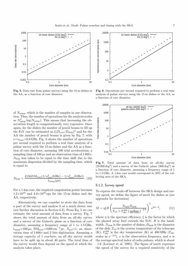
Fig. 5 shows the data rate from a pulsar survey for the15-m dishes and the AA as a function of core diame-ter, assuming tsamp=100µs, DMmax=1000 cm−3 pc for thedishes and DMmax=500 cm−3 pc for the AA, Npol=1 and2 bit digitisation. The AA was assumed to operate onthe full frequency range of 0.5 to 0.8GHz. The frequencyrange for the dishes was assumed to be 1 to 1.5GHz. Fora 1-km core, the data rate for the 15-m dishes with single-pixel feed is 4.7 × 1011 bytes per second and for the AAit is 1.6 × 1012 bytes per second. Both values scale lin-early with the FoV. We can estimate the number of oper-ations to search one ‘pencil beam’ for accelerated periodicsources as one Fourier Transform of all the samples in theobservation, for each trial DM-value and for each trial ac-celeration:

Noa = NDMNacc × 5Nsamp log2(Nsamp), (9)

where NDM is the number of trial DM-values, Nacc is thenumber of trial accelerations which scales with the square


0.001

0.01

0.1

1

10

100

1000

0.1 1 10

Dat

a ra

te (

tera

-byt

es/s

)

Core diameter (km)

15 meter dishes (0.64 deg2)AA (3 deg2)

Fig. 5. Data rate from pulsar surveys using the 15-m dishes orthe AA, as a function of core diameter.

of Nsamp, which is the number of samples in one observa-tion. Thus, the number of operations for the analysis scalesas N3

samp log(Nsamp). This means that increasing the ob-servation length is computationally very expensive. Onceagain, for the dishes the number of pencil beams to fill upthe FoV can be estimated as ξ(Dcore/Ddish)

2 and for theAA the number of pencil beams is given by Eq. 7, withν=νmax=0.8GHz. Fig. 6 shows the number of operationsper second required to perform a real time analysis of apulsar survey with the 15-m dishes and the AA as a func-tion of core diameter, assuming 100 trial accelerations, asampling time of 100µs and an observation time of 1 800 s.NDM was taken to be equal to the time shift due to themaximum dispersion divided by the sampling time, whichis equal to

NDM =4150DMmax(1/ν2

min(GHz) − 1/ν2max(GHz))

tsamp(µs). (10)

For a 1-km core, the required computation power becomes1.2×1016 and 4.0×1016 ops for the 15-m dishes and theAA, respectively.

Alternatively, we can consider to store the data froma part of the survey and analyse it at a much slower rate(see further discussion in Section 6.2). From Eq. 5 we canestimate the total amount of data from a survey. Fig. 7shows the total amount of data from an all-sky surveyand a survey of the Galactic plane as a function of corediameter, assuming a frequency range of 1 to 1.5GHz,tsamp=100µs, DMmax=1000 cm−3 pc, Npol=1, an obser-vation time of 1 800 s and 2 bits digitisation. Assuming astorage capacity of 1 exa-byte, an all sky survey wouldhave to be split up in about 40 parts. The total time ofthe survey would then depend on the speed at which theanalysis takes place.

0.1

1

10

100

1000

10000

0.1 1 10

Ope

ratio

ns p

er s

econ

d (p

eta-

ops)

Core diameter (km)

15 meter dishes (0.64 deg2)AA (3 deg2)

Fig. 6. Operations per second required to perform a real timeanalysis of pulsar surveys using the 15-m dishes or the AA, asa function of core diameter.

0.01

0.1

1

10

100

1000

10000

0.1 1 10

Tot

al d

ata

(exa

-byt

es)

Core diameter (km)

all-sky (30000 deg2)galactic plane (900 deg2)

Fig. 7. Total amount of data from an all-sky survey(35 000 deg2) and a survey of the Galactic plane (900 deg2) asa function of core diameter, assuming a frequency range of 1to 1.5 GHz. A 1-km core would correspond to 20% of the col-lecting area of the SKA.

5.1.2. Survey speed

To express the trade-off between the SKA design and sur-vey speed, we define the figure of merit for dishes as (seeappendix for derivation)

M = ηξB

(

NdishDdish

Ttel + T 400sky

(

ν400 MHz

)−2.6

)2

ν2α−2, (11)

where η is the aperture efficiency, ξ is the factor by whichthe phased array feed extends the FoV, B is the band-width, Ndish is the number of dishes, Ddish is the diameterof the dish, Ttel is the system temperature of the telescope(K), T 400

sky is the sky temperature (K) at 400MHz (Tsky

scales as ν−2.6), ν is the observation frequency, and α isthe average spectral index of radio pulsars, which is about–1.6 (Lorimer et al. 1995). The figure of merit expressesthe speed of the survey for a required sensitivity of the


1e-06

1e-05

1e-04

0.001

0.01

0.1

1

10

100

1000

0.1 1 10

Fig

ure

of m

erit

(arb

itrar

y un

its)


Fig. 8. The frequency dependence of the figure of merit. Thisfunction expresses the speed of the survey for a fixed sensitivityof the telescope.

telescope. Fig. 8 shows the strong dependence of the fig-ure of merit on the observation frequency. The slope athigh frequencies is due to the spectral index of pulsarsand the decrease of the FoV. At low frequency the figureof merit becomes flat as the sky temperature begins todominate the system temperature. In practise, pulsars be-come harder to detect at low frequencies where scatteringeffects broaden the pulsar profile. Since the scattering de-pends on the location on the sky, it was not included inthe merit function. Thus, at low frequencies the figure ofmerit is overestimated. However, scattering effects are onlysignificant for pulsars located in the Galactic plane. Fornormal pulsars, low frequencies are very favourable (seevan Leeuwen & Stappers 2008).

The total observation time of a survey is given by:

ttotal =Ωsur

ΩFoV

tpoint (12)

where Ωsur is the total solid angle of sky covered by thesurvey, ΩFoV is the total FoV of the dishes and tpoint isthe observation time per pointing.

6. Suggestions

An estimate of the computational power by 2015 is givenby Cornwell (2005) to be 10Pflop for $100M. To estimatewhat the SKA can achieve for pulsar searches and tim-ing, we will assume that several 1016 ops are available forbeam forming and data analysis when this survey will beperformed, which will be after 2020.

We consider three scenarios, two with full coherentbeam forming, where the analysis takes place either inreal time or offline and one scenario where part of thebeam forming takes place incoherently.

6.1. Real time analysis

First we assume that the analysis takes place equally fastas the data streaming in. The immediate benefits are that

no time is lost for the data analysis and that only reduceddata needs to be stored. One drawback, however, is thatthe data can only be processed once. Experience with cur-rent pulsar surveys show that it is extremely advantageousto have multiple passes at pulsar survey data analysis (seee.g. Faulkner et al. 2005).

As calculated in section 5.1.1, for a 1-km core thedata rate from the dishes with a single-pixel feed is4.7 × 1011 bytes/s. The required computational power forreal time analysis is 1.2 × 1016 ops. Both values scale lin-early with FoV. Only with SKA implementation B, wherethe dishes have phased array feeds, can the FoV of thedishes be increased beyond 0.64 deg2. Using the 1-km coreof the AA and using a FoV of 3 deg2 leads to a data rateof 1.6× 1012 bytes/s and requires a computation power of4.0 × 1016 ops to analyse the data in real time.

SKA implementation A suggests the all-sky survey tobe performed with single-pixel 15-m dishes. At low fre-quencies the FoV of the dishes is about 1 deg2. The entiresurvey will then take about 600 days. In implementation Ba larger FoV can be used. The survey time of 600 days thenscales inversely with the FoV, however the data rates andrequired computation power go up linearly with the FoV.Implementation C has the benefit of the AA for which anall-sky survey takes only about 200 days and the surveyof the Galactic plane with single-pixel 15-m dishes takesabout 30 days. The data rates and required computationpower for the AA are larger than for the dishes. Whenwe take this into account the total survey time for allimplementations become similar, except that implemen-tations B and C allow for a faster survey and the AA inimplementation C might be used for other observationssimultaneously (see Cordes 2007, for using the SKA as asynoptic survey telescope).

6.2. Offline analysis

The offline analysis requires the full data from an obser-vation to be stored. Thus, the data rates from Fig. 5 be-come the rates at which data is written to a storage de-vice. When the maximum data storage has been reached,the observation can be stopped and the data analysis canbe performed at any pace suitable. After the data analysishas been completed, the next observation can be run. Thisallows a trade-off between computation cost and surveyspeed. A drawback is that, depending on available futurestorage solutions, the total survey time may easily becomemore than a decade for any SKA implementation.

6.3. Incoherent beam forming

For real time analysis, restrictions on the computationalpower and data rate will likely limit the FoV to about3 deg2. The survey time will then become at least 200 days.Offline analysis requires the huge data rates to be writtento a storage device and will increase the survey time bya significant factor. We therefore consider the possibility


of incoherent addition of the sub arrays, as described insection 5.1.

We will assume that all the elements in the SKA areplaced such that their signals can be combined to formsub-arrays (or stations in the case of the AA) of 60 metresin diameter (similar to van Leeuwen & Stappers 2008, forLOFAR). The pencil beams that are formed by coherentlyadding the signals from the sub-array elements are about17 times larger than the pencil beams from coherentlybeam forming the 1-km core. Thus the number of pencilbeams required to fill the FoV becomes about 280 timessmaller. The computational requirements for beam form-ing, data analysis as well as the data rates go down linearlyby this factor. This method of beam forming utilises thefull collecting area of the SKA, which increases the sensi-tivity by a factor of 5. However, because the sub-arrays areadded incoherently, the sensitivity decreases by the squareroot of the number of sub-arrays. For the AA there willbe about 180 stations. Thus the sensitivity goes down bya factor of

√180/5 ≈ 2.7. Assuming that the dishes are

placed in sub-arrays with a 20% filling factor, the numberof sub-arrays will be between 600 and 900, depending onthe SKA implementation. For incoherent beam formingthe sensitivity will then go down by a factor between 5and 6.

7. Summary

We have investigated the pulsar yields for different SKAconfigurations by simulating SKA pulsar surveys for dif-ferent collecting areas and centre frequencies. For theGalactic plane, the optimal centre frequency lies justabove 1 GHz. Outside the Galactic plane the optimal cen-tre frequency lies between 600 and 900MHz, dependingon the collecting area. Combining the dishes and the AAto perform a survey inside the Galactic plane and outsidethe Galactic plane, respectively, would result in detectionof roughly 15 000 pulsars. Increasing the collecting areawithin the 1-km core would improve the detected numberof pulsars significantly.

Performing a pulsar survey with the SKA requires thecoherent addition of the signals of the individual elements,forming sufficient pencil beams as to fill the entire FoVof a single dish. Because of the extreme computationalrequirements that arise due to large baselines, it is notpossible to combine the signals of all of the elements inthe SKA. Rather, only the core of the SKA can be usedfor a pulsar survey. We have derived the computationalrequirements to perform such beam forming as a functionof core-diameter for the 15-m dishes and the AA. For a 1-km core the requirements are 2.2×1015 and 1.4×1014 opsfor the 15-m dishes and the AA, respectively. When thedishes are placed such that they can form sub-arrays, thecomputational requirement for beam forming goes downsignificantly. We have also calculated the data rates andthe computational requirements for applying a search-algorithm to the data to find binary pulsars. Both limit

the usage of the SKA for pulsar searches to a core of about1 km.

Acknowledgements. The authors would like to thank SimonJohnston, Andrew Lyne and Scott Ransom for their usefulsuggestions. This effort/activity is supported by the EuropeanCommunity Framework Programme 6, Square Kilometre ArrayDesign Studies (SKADS), contract no 011938. DRL is sup-ported by a Research Challenge Grant from West VirginiaEPSCoR.

Appendix

Beam forming of the dishes

Cordes (2007) estimated the number of operations to performthe beam forming for a pulsar survey as one operation (corre-sponding to the phase shift of one element) for each dish andeach polarisation at the Nyquist frequency. This needs to beperformed for each of the pencil beams that fill the total FoV.This leads to the total number of operations per second

Nosb = FcNdishNpolB(

Dcore

Ddish

)2

, (13)

where Fc is the fraction of dishes inside the core, Ndish is thetotal number of dishes, Npol is the number of polarisations,B is the bandwidth, Ddish is the diameter of the dishes andDcore is the diameter of the core. The fraction (Dcore/Ddish)2

is equal to the required number of pencil beams to fill up theFoV. If we assume that the dishes in the core are positionedsuch that they can form sub-arrays, beam forming can takeplace in two stages. In the first stage beam forming of the fullFoV is performed for each sub-array. In the second stage thefinal pencil beams are formed by coherently adding the cor-responding beams of each sub-array formed in the first stage.This leads to the following expression for the number of oper-ations required for beam forming in two stages:

Nosb2 = NsaNdishsaNpolB(

Dsa

Ddish

)2

+(

Dsa

Ddish

)2

NsaNpolB(

Dcore

Dsa

)2

, (14)

where Nsa is the number of sub-arrays in the core, Ndishsa is thenumber of dishes in one sub-array and Dsa is the diameter ofthe sub-arrays. Substituting Ndishsa = FcNdish/Nsa and Nsa =(Dcore/Dsa)

2 yields

Nosb2 = FcNdishNpolB(

Dsa

Ddish

)2

+NpolB(

Dcore

Ddish

)2 (Dcore

Dsa

)2

, (15)

which has a minimum at Dsa = Dcore(FcNdish)−1/4. At thisminimum, the number of operations for beam forming in 2stages is:

Nminosb2 = 2

√FcNdishNpolB

(

Dcore

Ddish

)2

. (16)

Beam forming of the AA

For the AA, initial beam forming will be performed at eachstation; this will lead to beams equivalent to those of a 60-m dish. Assuming a collecting area of 500 000 m2, this leads


to about 177 stations. The FoV of 1 pencil beam is givenby (λ/DCore)

2 = (c/νDcore)2 steradians, where c is the speed

of light. Thus, to cover 3 deg2 the required number of pencilbeams is (3π/180)2/(c/νDcore)

2. Within the frequency band,the number of pencil beams needs to remain identical as to en-able summing over frequency. In order to have a full coverageof the 3 deg2, the required number of pencil beams is thereforeobtained by setting ν to νmax. The number of operations persecond to perform the beam forming of the AA is then givenby (see also Eq. 3)

Nosb = FcNdishNpolB · 3(

π

180c

)2

D2coreν

2max. (17)

Derivation of figure of merit

Neglecting numerical factors and physical constants, the figureof merit expresses the speed of a survey for a given sensitivityof the telescope. It therefore scales with aperture efficiency (η),the FoV, the bandwidth (B), the square of the collecting area(A) and the reciprocal of the square of the system temperature(Tsys). For a pulsar survey it also scales with the square ofthe flux of pulsars, which scales as να, with ν the observationfrequency and α the average spectral index of radio pulsars,which is about –1.6. Thus:

M = ηBFoV

(

Aνα

Tsys

)2

. (18)

The FoV is given by ξλD−1dish

, where ξ is the factor by which thephased array feed extends the FoV and Ddish is the diameter ofthe antennas. This is equal to ξcν−1D−1

dish. The collecting areacan be expressed as A = NdishπD2

dish/4, where Ndish is thenumber of dishes. Tsys is the sum of the telescope temperatureand the sky temperature, the latter scaling with frequency asν−2.6. Putting all this in Eq. 18 and removing all constants,yields:

M = ηξB

(

NdishDdish

Ttel + T 400sky

(

ν400 MHz

)

−2.6

)2

ν2α−2 (19)

Glossary

The following list summarises the meaning of the most impor-tant parameters in this paper.

Tsys: system temperature (including contributions from re-ceiver and sky background.

T 400sky : sky temperature at 400 MHz.

FoV: Field-of-View, size of the sky area instantaneously cov-ered by the telescope.

η: aperture efficiency for dishes.Ddish: diameter of a single dish.Dtel: diameter of the total telescope (maximum baseline).Dcore: diameter of the core region.Nosb: number of operations per second required for beam

forming.Ndish: total number of dishes.Fc: fraction of the number of dishes inside the core.Npol: number of polarisations.B: observing bandwidth.ξ: factor by which the phased array feed expands the FoV.

Note that for a phased array feed this factor is frequencydependent.

νmax: maximum observing frequency.a, b: parameters appearing in Eq. 4.Ddish: survey data rate for one pencil beam.DAA: total survey data rate for AAs.tsamp: sampling time for pulsar survey.∆ν: channel bandwidth for pulsar survey.Nbits: number of bits used for digitisation of survey data.νmin: lowest frequency used for pulsar survey.DMmax: maximum dispersion measure to be searched or ex-

pected.NDM: number of trial DM-values.Nsamp: number of samples in each survey time series.Nacc: number of trial accelerations to be searched.NpbAA: number of pencil beams for AAs.Noa: number of operations to search one pencil beam in accel-

eration searches.M : survey-speed figure-of-merit for searches with dishes.ttotal: total observing time for a survey.tpoint: observing time per survey pointing.Ωsur: total sky (solid angle) for survey.ΩFoV: total FoV for dishes.

References

Cordes, J. 2007, SKA memo 97, http://www.skatelescope.org/PDF/memos/97 memo Cordes.pdf

Cordes, J. M., Kramer, M., Lazio, T. J. W., et al. 2004, NewAstronomy Review, 48, 1413

Cordes, J. M. & Lazio, T. J. W. 2002, ArXiv Astrophysicse-prints

Cornwell, T. J. 2005, SKA memo 64Faucher-Giguere, C.-A. & Kaspi, V. M. 2006, ApJ, 643, 332Faulkner, A. J., Kramer, M., Lyne, A. G., et al. 2005, ApJ,

618, L119Helfand, D. J., Manchester, R. N., & Taylor, J. H. 1975, ApJ,

198, 661Hulse, R. A. & Taylor, J. H. 1975, 201, L55Ivashina, M. V., bij de Vaate, J. G., Braun, R., & Bregman,

J. D. 2004, in Presented at the Society of Photo-OpticalInstrumentation Engineers (SPIE) Conference, Vol. 5489,Ground-based Telescopes. Edited by Oschmann, JacobusM., Jr. Proceedings of the SPIE, Volume 5489, pp. 1127-1138 (2004)., ed. J. M. Oschmann, Jr., 1127–1138

Kramer, M., Backer, D. C., Cordes, J. M., et al. 2004, NewAstronomy Review, 48, 993

Kramer, M., Lyne, A. G., O’Brien, J. T., Jordan, C. A., &Lorimer, D. R. 2006, Science, 312, 549

Lorimer, D. R., Faulkner, A. J., Lyne, A. G., et al. 2006,MNRAS, 372, 777

Lorimer, D. R. & Kramer, M. 2005, Handbook of PulsarAstronomy (Cambridge University Press)

Lorimer, D. R., Yates, J. A., Lyne, A. G., & Gould, D. M.1995, MNRAS, 273, 411

McLaughlin, M. A., Lyne, A. G., Lorimer, D. R., et al. 2006,439, 817

Schilizzi, R. T., Alexander, P., Cordes, J. M., et al.2007, SKA draft, http://www.skatelescope.org/PDF/

Preliminary Specifications of the Square Kilometre Array

v2.7.1.pdf

Terzian, Y. & Lazio, J. 2006, in Presented at theSociety of Photo-Optical Instrumentation Engineers (SPIE)Conference, Vol. 6267, Ground-based and AirborneTelescopes. Edited by Stepp, Larry M.. Proceedings of theSPIE, Volume 6267, pp. 62672D (2006).


van Leeuwen, J. & Stappers, B. 2008, in American Institute ofPhysics Conference Series, Vol. 983, American Institute ofPhysics Conference Series, 598–600

van Straten, W. 2006, ApJ, 642, 1004

pulsar searches and timing with the ska - skads-eu.org · the square kilometre array (ska) is a...

Documents