q. changeat, b. edwards, i.p. waldmann, andg. tinetti
TRANSCRIPT
Draft version October 12, 2020Typeset using LATEX twocolumn style in AASTeX62
Towards a more complex description of chemical profiles in exoplanet retrievals: A 2-layer parameterisation
Q. Changeat,1 B. Edwards,1 I.P. Waldmann,1 and G. Tinetti1
1Department of Physics and Astronomy
University College London
Gower Street,WC1E 6BT London, United Kingdom
(Accepted to ApJ, November 2019)
ABSTRACT
State of the art spectral retrieval models of exoplanet atmospheres assume constant chemical profiles
with altitude. This assumption is justified by the information content of current datasets which do not
allow, in most cases, for the molecular abundances as a function of pressure to be constrained.
In the context of the next generation of telescopes, a more accurate description of chemical profiles
may become crucial to interpret observations and gain new insights into atmospheric physics. We
explore here the possibility of retrieving pressure-dependent chemical profiles from transit spectra,
without injecting any priors from theoretical chemical models in our retrievals. The “2-layer” param-
eterisation presented here allows for the independent extraction of molecular abundances above and
below a certain atmospheric pressure.
By simulating various cases, we demonstrate that this evolution from constant chemical abundances
is justified by the information content of spectra provided by future space instruments. Comparisons
with traditional retrieval models show that assumptions made on chemical profiles may significantly
impact retrieved parameters, such as the atmospheric temperature, and justify the attention we give
here to this issue.
We find that the 2-layer retrieval accurately captures discontinuities in the vertical chemical profiles,
which could be caused by disequilibrium processes – such as photo-chemistry – or the presence of
clouds/hazes. The 2-layer retrieval could also help to constrain the composition of clouds and hazes
by exploring the correlation between the chemical changes in the gaseous phase and the pressure at
which the condensed phase occurs.
The 2-layer retrieval presented here therefore represents an important step forward in our ability to
constrain theoretical chemical models and cloud/haze composition from the analysis of future obser-
vations.
1. INTRODUCTION
In the past years an increasing number of exoplanetary
atmospheres have been characterised with space and
ground-based observatories. Ultraviolet, optical and in-
frared spectra, recorded through transit, eclipse, high-
dispersion and direct imaging, have offered a glimpse
of the atmospheric structure and composition of exotic
worlds orbiting other stars. In most cases the data
available are sparse and therefore their interpretation
is rarely unique. To explore the degeneracy, reliability
and correlations among the atmospheric parameters ex-
tracted from the data, the past decade has seen a surge
Corresponding author: Q. Changeat
in spectral retrieval models developed by many teams
(e.g. Terrile et al. 2005; Irwin et al. 2008; Madhusudhan
& Seager 2009; Line et al. 2013; Waldmann et al. 2015b;
Cubillos et al. 2016; Lavie et al. 2017; Goyal et al. 2018;
Gandhi & Madhusudhan 2018).
Most current spectral retrieval models assume con-
stant or simplified atmospheric thermal profiles. Addi-
tionally, chemical profiles which are constant with al-
titude are assumed (e.g. MacDonald & Madhusudhan
2017; Tsiaras et al. 2018; Pinhas et al. 2019). In these
models, the mixing ratio of each individual molecule is
fully determined by a single free parameter. So far, this
approach has been successful due to the relatively poor
quality of the input data from space and ground-based
instruments. Given the low signal to noise, spectral res-
olution and the narrow wavelength coverage, current
arX
iv:1
903.
1118
0v4
[as
tro-
ph.E
P] 9
Oct
202
0
2
data cannot be used to constrain more complex mod-
els. However, the next generation of telescopes coming
online in the next decade, will demand more complex re-
trievals to extract all the information content embedded
in the data. In the context of NASA-JWST (Bean et al.
2018), ESA-ARIEL (Tinetti et al. 2018) and other facil-
ities from ground and space (e.g. E-ELT (Brandl et al.
2018), Twinkle (Edwards et al. 2019b)), the higher res-
olution, signal-to-noise ratio (SNR) and broader wave-
length range will allow for less abundant trace gases
and refined thermal profiles to be captured. For in-
stance, Rocchetto et al. (2016) have demonstrated that
the assumption of constant atmospheric thermal profiles
will be inadequate to interpret correctly future better-
quality transit spectra recorded from space. Addition-
ally these new instruments may be sensitive enough to
constrain non-constant chemical profiles.
The need for an increased chemical complexity is
sometimes addressed in the literature through addi-
tional constraints in the retrievals from dynamical and
chemical models (“hybrid” models). This method is al-
ready widely explored in retrievals aiming at constrain-
ing the thermal profiles, e.g. the Guillot model (Guillot
2010) and other 2-stream approximations (Heng et al.
2014; Malik et al. 2017). This strategy allows for more
complex thermal profiles to be considered, while limit-
ing the number of free parameters. Similarly, equilib-
rium and disequilibrium chemical models may be used
to constrain chemical profiles. Agundez et al. (2014)
showed, with their 2D chemical model of HD 209458 b
and HD 189733 b, that accurate parameterisations of ex-
oplanetary atmospheres could be extremely complex.
Interesting alternatives combine both physical/chemical
models and free parameters such as the model adopted
by Madhusudhan & Seager (2009), where the chemical
profiles are computed in equilibrium and multiplied by
a factor to account for potential departures from the
equilibrium.
The hybrid retrieval models have, however, two major
disadvantages. First, the forward model requires signifi-
cant computing time to ensure convergence of the chem-
ical/dynamical modules, which becomes even longer if
used for retrievals. More fundamentally, they imply
assumptions on the state of the planet and its physi-
cal/chemical behaviour. As the physics of such systems
can be extremely complex and far from any environment
we know in the Solar System, the selection of a particu-
lar model may lead to results biased by preconception.
For instance, Venot et al. (2012) proposed a disequi-
librium model adapted for hot-Jupiters and found sig-
nificant differences when comparing with other models
such as the equilibrium ones. This result highlights the
issue of assuming a particular physics as a prior in in-
verse models, when our knowledge of exoplanetary at-
mospheres is still in an early phase. At least until our
knowledge of these exotic worlds has progressed substan-
tially, the results obtained by spectral retrievals should
be kept independent from ab initio dynamical and chem-
ical models, and used instead to constrain/validate some
aspects of said models.
The approach taken here is to increase the number of
free variables for each molecular species considered. Ap-
plying this approach to currently available data is not
justifiable as it would simply increase the degeneracy of
the retrieved solutions. By contrast, attempts to use
models of inadequate complexity to analyse spectra ob-
served by next generation facilities are likely to provide
incomplete pictures and misleading results. This paper
explores the importance of moving towards a more com-
plete description of chemical profiles through the anal-
ysis of simulated transit data from JWST, ARIEL and
other future telescopes. In that context, we consider the
example of a 2-layer parametrisation with 3 degrees of
freedom.
Section 2 presents the 2-layer approach and describes
the methodology adopted. A validation of the method
using simple cases is then reported in Section 3, fol-
lowed by specific examples of exoplanetary atmospheres
in section 4. Section 5 discusses the model’s strengths
and limitations.
2. METHODOLOGY
2.1. Overview and key assumptions
This work focuses on retrievals of transit spectra, so
that, for simplicity, the thermal profile can be assumed
isothermal in some benchmark cases – note that this as-
sumption is abandoned in Section 4 to ensure our simula-
tions are as realistic as possible. In eclipse spectroscopy,
the thermal gradients and the chemical profiles are al-
ways entangled, making it a more complex case which
will be considered in a separate paper.
The 2-layer parametrisation has been adopted for its
simplicity and because it does not rely on external phys-
ical assumptions which, as previously described, could
bias the results of the retrieval. While our model is
clearly not representative of all real atmospheres, it al-
lows us to consider a departure from the constant mixing
ratios case.
Both the forward radiative transfer models and the
inverse models (spectral retrievals) are based on the
open-source TauREx from Waldmann et al. (2015a) and
Waldmann et al. (2015b), which has been modified for
the purpose of this study. TauREx is a fully Bayesian
radiative transfer and retrieval framework which en-
3
Opacity References
H2-H2 Abel et al. (2011), Fletcher et al. (2018)
H2-He Abel et al. (2012)
H2O Barton et al. (2017), Polyansky et al. (2018)
CH4 Hill et al. (2013), Yurchenko & Tennyson (2014)
CO Li et al. (2015)
CO2 Rothman et al. (2010)
TiO Schwenke (1998)
Table 1. List of opacities used in this work
compasses molecular line-lists from the Exomol project
(Tennyson et al. 2016), HITEMP (Rothman & Gordon
2014) and HITRAN (Gordon et al. 2016). The com-
plete list of opacity used in this paper can be found in
Table 1. The public version of TauREx1 is able to re-
trieve chemical composition of exoplanets by assuming
constant abundances with altitude. It can also simulate
atmospheres in equilibrium.
Here we added the new 2-layer module to the code.
The chemical parametrisation we used can be described
by three variables: the surface/bottom abundance XS ,
the top abundance XT and the pressure defining the
separation of the two layers (Input Pressure Point PIfor the forward model and Retrieved Pressure Point PR).
The chemical profile is linearly interpolated in log space
– smoothing over 10% of the atmosphere – to avoid a
sharp transition in the profile. An example of a 2-layer
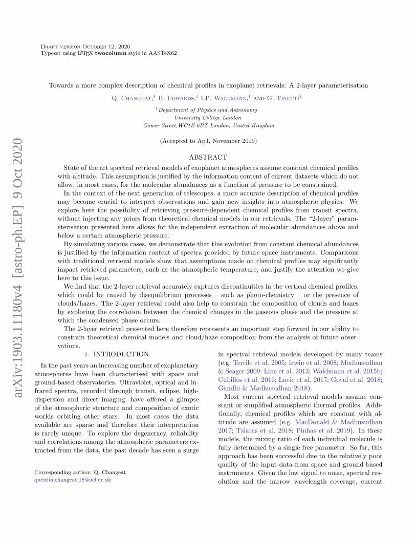
chemical profile for water vapour is given in Figure 1.
For all the tests reported in this paper, we follow the
3-step procedure detailed below.
2.2. Step 1: generating high-resolution input spectra
We start by using TauREx in forward mode and gener-ate a high-resolution theoretical spectrum. In our mod-
els, we assumed a maximum pressure of 10 bar, cor-
responding to the planet surface. The atmosphere is
composed of the inactive gases H2 and He, for which
we set the ratio He/H2 to 0.15 and add the considered
active molecules (relative abundance defined by their
mixing ratio). We consider collision induced absorption
of the H2-H2 and H2-He pairs and opacities induced by
Rayleigh scattering (Cox 2015). Throughout the paper,
the molecular mixing ratios and profiles in the forward
model are varied to create high resolution spectra for a
wide range of compositions and cases. The planetary
parameters have been set to the well known exoplanet
HD 209458 b in Section 3 and are listed in the Appendix.
1 https://github.com/ucl-exoplanets/TauREx public
10 10 10 9 10 8 10 7 10 6 10 5 10 4 10 3
Mixing ratio of H2O
10 9
10 7
10 5
10 3
10 1
101
Pres
sure
(bar
)
Figure 1. Example of a 2-layer chemical profile withH2O. This profile can be used as input for forward simu-lations of exoplanet spectra, as well as for fitting data inretrievals. Here, the surface layer is depleted with a mix-ing ratio XS(H2O) of 10−10 and the top layer has a largequantity of H2O, with XT (H2O) = 10−3. The separationpressure of the two layers is set to PI(H2O) = 10−3 bar andthe transition is smoothed over 10% of the atmosphere (10layers).
The adopted approach is compatible with any other set
of planetary and atmospheric parameters and is applied
in section 4 to two other simulated planets inspired by
WASP-33 b and GJ 1214 b.
2.3. Step 2: convolution of the input spectra with the
instrument response function
High-resolution theoretical spectra obtained in sec.
2.2 are convolved with the instrument response func-
tion to simulate realistic observations. We use ArielRad
(Mugnai et al. 2020) to provide realistic noise models
for spectra obtained by ARIEL and chose planets that
are in the current target list Edwards et al. (2019a).
In the case of JWST, we used the noise estimates for
HD 209458 b presented in Rocchetto et al. (2016). An
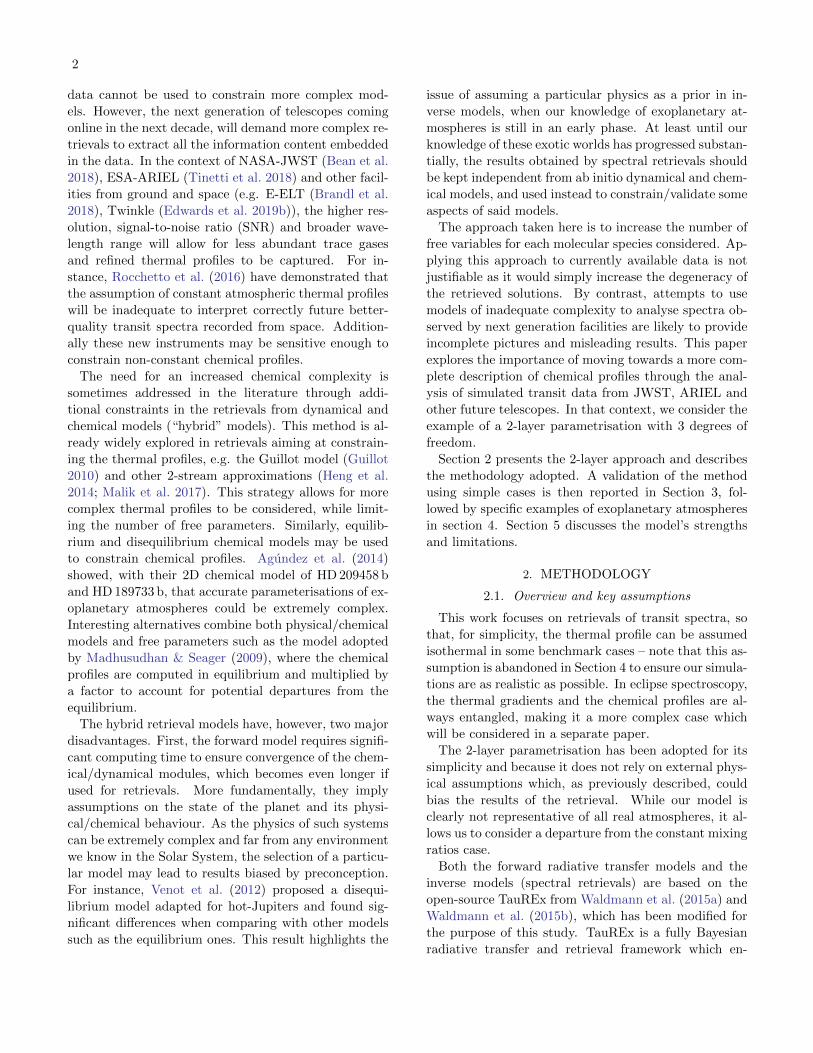
example of this process is shown in Figure 2 where
both the high-resolution theoretical spectrum and the
ARIEL-simulated case are presented.
2.4. Step 3: Retrievals
We run TauREx in retrieval mode and use the spectra
obtained in step 2 as input to the retrieval. We used the
nested sampling algorithm Multinest from Feroz et al.
(2009) with 1500 live points and a log likelihood tol-
erance of 0.5. The retrieved parameters include our
chemical setup (3 variables per chemical species), the
isothermal temperature value and the planet radius. We
4
Figure 2. Example of forward models assuming a 2-layerchemical profile of H2O as shown in Figure 1. Grey curve:high-resolution theoretical spectrum obtained with TauRExat step 1 (sec. 2.2). Blue curve: simulated ARIEL observa-tions after having processed the theoretical spectrum in step2 (sec. 2.3).
therefore have a minimum of 5 free parameters that we
attempt to retrieve. In the case where the mixing ra-
tios were assumed constant with altitude (1-layer for-
ward model), the Retrieved Pressure Point has been
fixed, so that we have only 2 free variables per chem-
ical species or a minimum of 4 free parameters. In
our retrieval scheme, we use uniform priors for all the
free parameters. In all our retrievals, chemical abun-
dances are allowed to explore the bounds 10−12 to 10−1.
For the Retrieved Pressure Point, we allow the bounds
from 10−1 to 10−4 bar for the Section 3. In Section
4, since we investigate less ad-hoc situations, we allow
the pressure to explore 10−1 bar to 10−7 bar. For the
isothermal temperature retrievals, the priors span ± 30
percent of the ground truth value. In section 4, since
we investigate more realistic examples, we retrieve a 3-
point temperature profile (Waldmann et al. (2015a)).
The atmospheric parameters used to generate the the-
oretical spectrum in step 1 are the ground truth. By
comparing the posteriors obtained by the retrieval to
the ground truth, we can test the reliability and ac-
curacy of the retrieval process. Furthermore, by using
the predicted performances of JWST and ARIEL, we
can quantify the expected information content of future
data, with a view to assessing the ability to probe the
chemical complexity of exoplanet atmospheres. For each
retrieval, we state the Nested Sampling Log-Evidence.
Bayes factor B (Jeffreys 1998), which is the ratio of the
evidences of two competing models (E1 and E2), allows
to compare models against each other. In practice, the
log(B) Interpretation
0 to 0.5 No Evidence
0.5 to 1 Some Evidence
1 to 2 Strong Evidence
> 2 Decisive
Table 2. Interpretation of the Bayes ratio (Kass & Raftery1995)
table in Kass & Raftery (1995) gives an interpretation
of log(B) = ∆log(E) = log(E2) − log(E1):
By applying the 3-step methodology, a number of
cases are simulated. Firstly, we verify that the 2-layer
retrieval is able to recover the more basic 1-layer input
(i.e. a constant chemical profile). We then investigate
the “retrievability” of the 2-layer input spectrum by a
2-layer retrieval in the case of JWST and ARIEL ob-
servations. Finally, we explore the advantage of using
a 2-layer approach by comparing how a 2-layer input
spectrum is recovered by both 1- and 2-layer retrievals.
2.5. Testing the 2-layer approach: Retrieval of a
1-layer input spectrum using the 2-layer
parametrisation
As a sanity check, we test that the more complex 2-
layer model can indeed recognise the simple case of con-
stant chemistry. A 1-layer simulated spectrum is gener-
ated and we attempt to recover the solution using the
2-layer model. Here, the retrieval of the pressure point
(PR) is disabled as this parameter introduces intrinsic
degeneracy in the specific case of constant chemistry.
Here, the goal being to illustrate that our 2-layer model
returns the expected solution when tested on the 1-layer
forward model, the behaviour of the retrieval when the
Retrieved Pressure Point is activated is discussed in sec-
tion 4. As any value for this point would work, we arbi-
trarily choose to set it at PI = 10−1.3 bar.
2.6. Retrieval of a 2-layer input spectrum as observed
by JWST and ARIEL
We study an exoplanet exhibiting noticeable chemical
modulations with altitude. This case can be simulated
by using a 2-layer profile as input. We present the partic-
ular case of an input H2O profile with 2 layers separating
at PI(H2O) = 10−2 bar. The input H2O surface layer is
set with a mixing ratio of XS(H2O) = 10−3 and the top
layer contains XT (H2O) = 10−5. The input spectrum
is simulated at high-resolution and observations are re-
produced by convolving the theoretical spectrum to the
instrument response function of JWST and ARIEL.
2.7. Comparison of the 1-layer and 2-layer retrievals.
5
By comparing the results obtained with the 1-layer
and 2-layer retrievals, we aim to illustrate issues that
may occur when performing a retrieval with a model of
inappropriate complexity. Therefore, we simulate plan-
etary atmospheres with 2-layer chemical profiles and
analyse the results if the retrieval is performed with a
1-layer chemical approach. For this test, we use ARIEL
simulations to illustrate our results. In particular, two
main issues could occur and need to be tested:
1. The observed spectrum cannot be explained using
the 1-layer retrieval, as the best solution retrieved
does not fit the data.
2. The 1-layer retrieval manages to achieve a “good”
fit but the retrieved parameters are wrong com-
pared to the ground-truth. This issue is more sub-
tle as there is little evidence and no direct way to
spot the error.
These two points can be tested by considering the fol-
lowing examples. For the former, we assume an atmo-
sphere with a single CH4 profile with a surface layer
of XS(CH4) = 10−5 up to PI(CH4) = 10−2 bar and
XT (CH4) = 10−10 above that pressure, corresponding
to a depleted layer. For the latter, we simulate a sin-
gle H2O profile where the planet contains XS(H2O) =
10−10 up to 10−2 bar and the mixing ratio isXT (H2O) =
10−3 for lower pressures.
3. RESULTS
3.1. Testing the 2-layer approach: Retrieval of a
1-layer input spectrum using the 2-layer
parametrisation
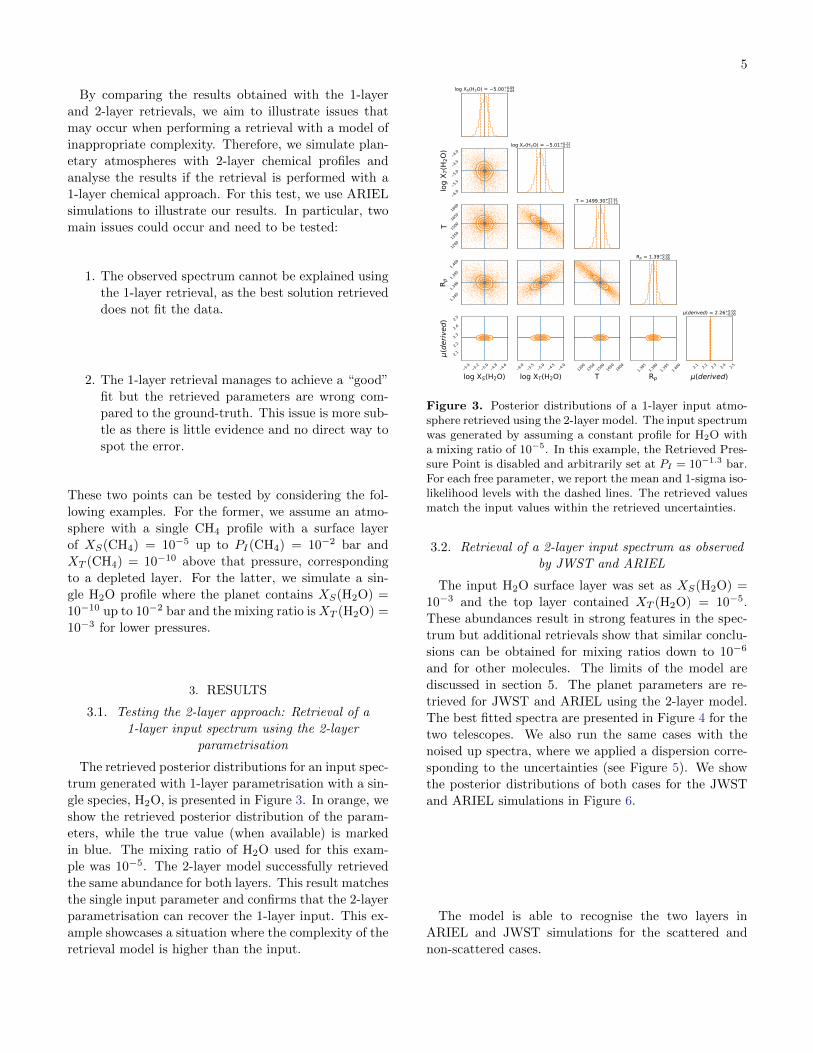
The retrieved posterior distributions for an input spec-
trum generated with 1-layer parametrisation with a sin-
gle species, H2O, is presented in Figure 3. In orange, we
show the retrieved posterior distribution of the param-
eters, while the true value (when available) is marked
in blue. The mixing ratio of H2O used for this exam-
ple was 10−5. The 2-layer model successfully retrieved
the same abundance for both layers. This result matches
the single input parameter and confirms that the 2-layer
parametrisation can recover the 1-layer input. This ex-
ample showcases a situation where the complexity of the
retrieval model is higher than the input.
log XS(H2O) = 5.00+0.090.09
6.05.55.04.54.0
log
X T(H
2O)
log XT(H2O) = 5.01+0.220.22
1200
1350
1500
1650
1800
T
T = 1499.30+57.6157.12
1.385
1.390
1.395
1.400
R p
Rp = 1.39+0.000.00
5.4 5.2 5.0 4.8 4.6
log XS(H2O)
2.12.22.32.42.5
(der
ived
)
6.0 5.5 5.0 4.5 4.0
log XT(H2O)12
0013
5015
0016
5018
00
T1.3
851.3
901.3
951.4
00
Rp
2.1 2.2 2.3 2.4 2.5
(derived)
(derived) = 2.26+0.000.00
Figure 3. Posterior distributions of a 1-layer input atmo-sphere retrieved using the 2-layer model. The input spectrumwas generated by assuming a constant profile for H2O witha mixing ratio of 10−5. In this example, the Retrieved Pres-sure Point is disabled and arbitrarily set at PI = 10−1.3 bar.For each free parameter, we report the mean and 1-sigma iso-likelihood levels with the dashed lines. The retrieved valuesmatch the input values within the retrieved uncertainties.
3.2. Retrieval of a 2-layer input spectrum as observed
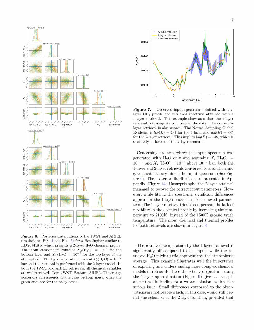
by JWST and ARIEL
The input H2O surface layer was set as XS(H2O) =
10−3 and the top layer contained XT (H2O) = 10−5.
These abundances result in strong features in the spec-
trum but additional retrievals show that similar conclu-
sions can be obtained for mixing ratios down to 10−6
and for other molecules. The limits of the model are
discussed in section 5. The planet parameters are re-
trieved for JWST and ARIEL using the 2-layer model.
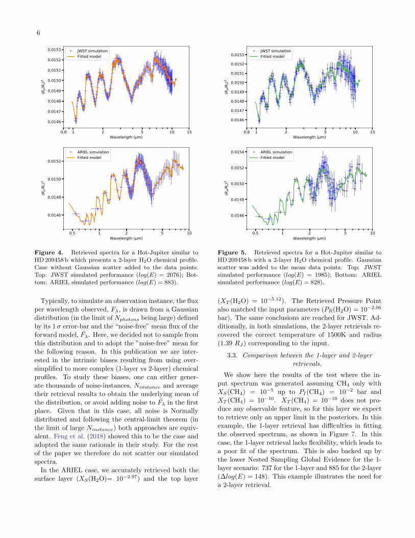
The best fitted spectra are presented in Figure 4 for the
two telescopes. We also run the same cases with the
noised up spectra, where we applied a dispersion corre-
sponding to the uncertainties (see Figure 5). We show
the posterior distributions of both cases for the JWST
and ARIEL simulations in Figure 6.
The model is able to recognise the two layers in
ARIEL and JWST simulations for the scattered and
non-scattered cases.
6
0.8 1 2 5 10 15Wavelength ( m)
0.0146
0.0147
0.0148
0.0149
0.0150
0.0151
0.0152
0.0153(R
p/Rs)2
JWST simulationFitted model
0.5 1 2 5 10Wavelength ( m)
0.0146
0.0148
0.0150
0.0152
(Rp/R
s)2
ARIEL simulationFitted model
Figure 4. Retrieved spectra for a Hot-Jupiter similar toHD 209458 b which presents a 2-layer H2O chemical profile.Case without Gaussian scatter added to the data points.Top: JWST simulated performance (log(E) = 2076); Bot-tom: ARIEL simulated performance (log(E) = 883).
Typically, to simulate an observation instance, the flux
per wavelength observed, Fλ, is drawn from a Gaussian
distribution (in the limit of Nphotons being large) defined
by its 1σ error-bar and the “noise-free” mean flux of the
forward model, Fλ. Here, we decided not to sample from
this distribution and to adopt the ”noise-free” mean for
the following reason. In this publication we are inter-
ested in the intrinsic biases resulting from using over-
simplified to more complex (1-layer vs 2-layer) chemical
profiles. To study these biases, one can either gener-
ate thousands of noise-instances, Ninstance and average
their retrieval results to obtain the underlying mean of
the distribution, or avoid adding noise to Fλ in the first
place. Given that in this case, all noise is Normally
distributed and following the central-limit theorem (in
the limit of large Ninstance) both approaches are equiv-
alent. Feng et al. (2018) showed this to be the case and
adopted the same rationale in their study. For the rest
of the paper we therefore do not scatter our simulated
spectra.
In the ARIEL case, we accurately retrieved both the
surface layer (XS(H2O)= 10−2.97) and the top layer
0.8 1 2 5 10 15Wavelength ( m)
0.0146
0.0147
0.0148
0.0149
0.0150
0.0151
0.0152
0.0153
(Rp/R
s)2
JWST simulationFitted model
0.5 1 2 5 10Wavelength ( m)
0.0146
0.0148
0.0150
0.0152
0.0154
(Rp/R
s)2
ARIEL simulationFitted model
Figure 5. Retrieved spectra for a Hot-Jupiter similar toHD 209458 b with a 2-layer H2O chemical profile. Gaussianscatter was added to the mean data points. Top: JWSTsimulated performance (log(E) = 1985); Bottom: ARIELsimulated performance (log(E) = 828).
(XT (H2O) = 10−5.12). The Retrieved Pressure Point
also matched the input parameters (PR(H2O) = 10−2.06
bar). The same conclusions are reached for JWST. Ad-
ditionally, in both simulations, the 2-layer retrievals re-
covered the correct temperature of 1500K and radius
(1.39 RJ) corresponding to the input.
3.3. Comparison between the 1-layer and 2-layer
retrievals.
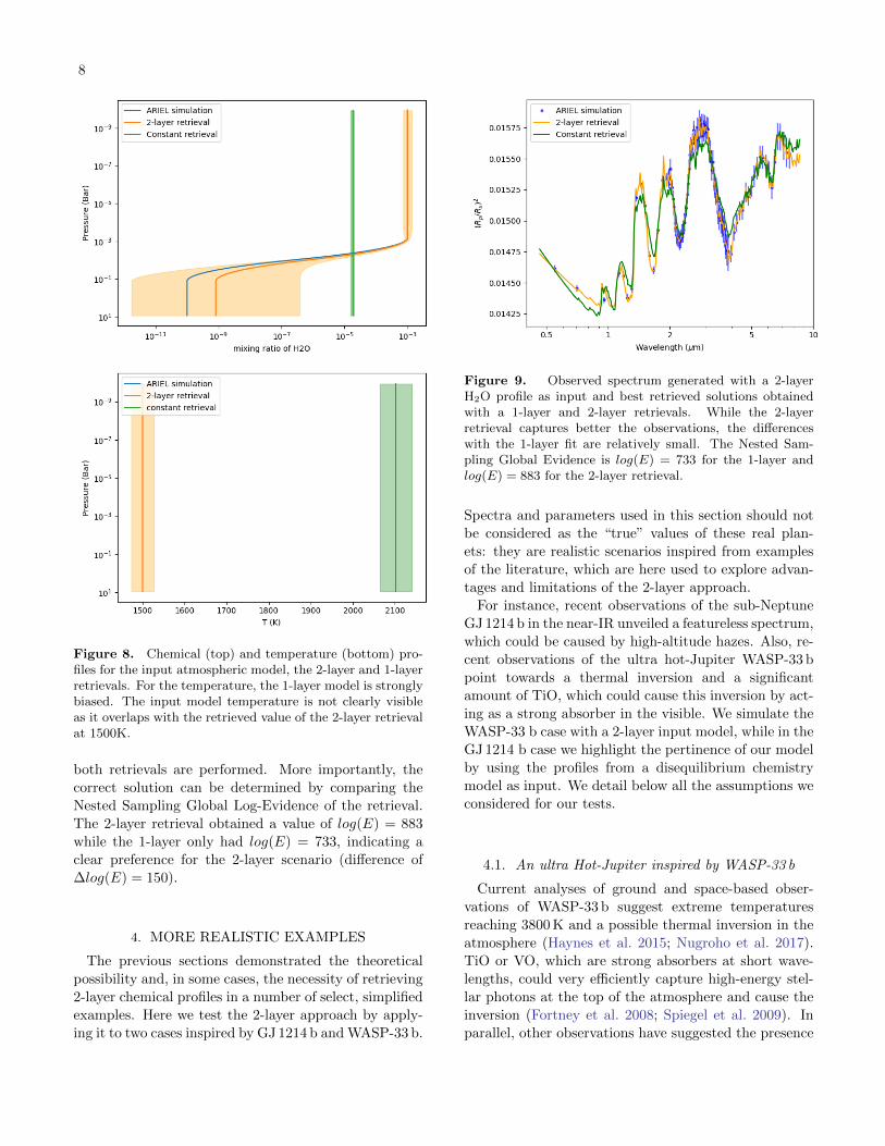
We show here the results of the test where the in-
put spectrum was generated assuming CH4 only with
XS(CH4) = 10−5 up to PI(CH4) = 10−2 bar and
XT (CH4) = 10−10. XT (CH4) = 10−10 does not pro-
duce any observable feature, so for this layer we expect
to retrieve only an upper limit in the posteriors. In this
example, the 1-layer retrieval has difficulties in fitting
the observed spectrum, as shown in Figure 7. In this
case, the 1-layer retrieval lacks flexibility, which leads to
a poor fit of the spectrum. This is also backed up by
the lower Nested Sampling Global Evidence for the 1-
layer scenario: 737 for the 1-layer and 885 for the 2-layer
(∆log(E) = 148). This example illustrates the need for
a 2-layer retrieval.
7
log XS(H2O) = 3.08+0.190.15
6.0
5.5
5.0
4.5
4.0
log
X T(H
2O) log XT(H2O) = 5.11+0.17
0.13
2.82.42.01.61.2
log
P(H 2
O)
log P(H2O) = 2.05+0.140.18
1200
1400
1600
1800
T
T = 1526.01+41.4939.55
1.380
1.386
1.392
1.398
R p
Rp = 1.39+0.000.00
4.0 3.5 3.0 2.5 2.0
log XS(H2O)
1.82.12.42.73.0
(der
ived
)
6.0 5.5 5.0 4.5 4.0
log XT(H2O)2.8 2.4 2.0 1.6 1.2
log P(H2O)12
0014
0016
0018
00
T1.3
801.3
861.3
921.3
98
Rp
1.8 2.1 2.4 2.7 3.0
(derived)
(derived) = 2.27+0.010.00
log XS(H2O) = 2.97+0.220.19
6.0
5.5
5.0
4.5
4.0
log
X T(H
2O) log XT(H2O) = 5.12+0.24
0.25
2.82.42.01.61.2
log
P(H 2
O)
log P(H2O) = 2.06+0.180.20
1200
1400
1600
1800
T
T = 1501.13+87.0979.84
1.380
1.386
1.392
1.398
R p
Rp = 1.39+0.000.00
4.0 3.5 3.0 2.5 2.0
log XS(H2O)
1.82.12.42.73.0
(der
ived
)
6.0 5.5 5.0 4.5 4.0
log XT(H2O)2.8 2.4 2.0 1.6 1.2
log P(H2O)12
0014
0016
0018
00
T1.3
801.3
861.3
921.3
98
Rp
1.8 2.1 2.4 2.7 3.0
(derived)
(derived) = 2.28+0.010.01
Figure 6. Posterior distributions of the JWST and ARIELsimulations (Fig. 4 and Fig. 5) for a Hot-Jupiter similar toHD 209458 b, which presents a 2-layer H2O chemical profile.The input atmosphere contains XS(H2O) = 10−3 for thebottom layer and XT (H2O) = 10−5 for the top layer of theatmosphere. The layers separation is set at PI(H2O) = 10−2
bar and the retrieval is performed with the 2-layer model. Inboth the JWST and ARIEL retrievals, all chemical variablesare well retrieved. Top: JWST; Bottom: ARIEL. The orangeposteriors corresponds to the case without noise, while thegreen ones are for the noisy cases.
Figure 7. Observed input spectrum obtained with a 2-layer CH4 profile and retrieved spectrum obtained with a1-layer retrieval. This example showcases that the 1-layerretrieval is inadequate to interpret the data. The correct 2-layer retrieval is also shown. The Nested Sampling GlobalEvidence is log(E) = 737 for the 1-layer and log(E) = 885for the 2-layer retrieval. This implies log(B) = 148, which isdecisively in favour of the 2-layer scenario.
Concerning the test where the input spectrum was
generated with H2O only and assuming XS(H2O) =
10−10 and XT (H2O) = 10−3 above 10−2 bar, both the
1-layer and 2-layer retrievals converged to a solution and
gave a satisfactory fits of the input spectrum (See Fig-
ure 9). The posterior distributions are presented in Ap-
pendix, Figure 14. Unsurprisingly, the 2-layer retrieval
managed to recover the correct input parameters. How-
ever, while fitting the spectrum, significant differences
appear for the 1-layer model in the retrieved parame-
ters. The 1-layer retrieval tries to compensate the lack of
flexibility in the chemical profile by increasing the tem-
perature to 2100K instead of the 1500K ground truth
temperature. The input chemical and thermal profiles
for both retrievals are shown in Figure 8.
The retrieved temperature by the 1-layer retrieval is
significantly off compared to the input, while the re-
trieved H2O mixing ratio approximates the atmospheric
average. This example illustrates well the importance
of exploring and understanding more complex chemical
models in retrievals. Here the retrieved spectrum using
the 1-layer approximation (Figure 9) gives an accept-
able fit while leading to a wrong solution, which is a
serious issue. Small differences compared to the obser-
vations are noticeable which, in this case, would still per-
mit the selection of the 2-layer solution, provided that
8
Figure 8. Chemical (top) and temperature (bottom) pro-files for the input atmospheric model, the 2-layer and 1-layerretrievals. For the temperature, the 1-layer model is stronglybiased. The input model temperature is not clearly visibleas it overlaps with the retrieved value of the 2-layer retrievalat 1500K.
both retrievals are performed. More importantly, the
correct solution can be determined by comparing the
Nested Sampling Global Log-Evidence of the retrieval.
The 2-layer retrieval obtained a value of log(E) = 883
while the 1-layer only had log(E) = 733, indicating a
clear preference for the 2-layer scenario (difference of
∆log(E) = 150).
4. MORE REALISTIC EXAMPLES
The previous sections demonstrated the theoretical
possibility and, in some cases, the necessity of retrieving
2-layer chemical profiles in a number of select, simplified
examples. Here we test the 2-layer approach by apply-
ing it to two cases inspired by GJ 1214 b and WASP-33 b.
Figure 9. Observed spectrum generated with a 2-layerH2O profile as input and best retrieved solutions obtainedwith a 1-layer and 2-layer retrievals. While the 2-layerretrieval captures better the observations, the differenceswith the 1-layer fit are relatively small. The Nested Sam-pling Global Evidence is log(E) = 733 for the 1-layer andlog(E) = 883 for the 2-layer retrieval.
Spectra and parameters used in this section should not
be considered as the “true” values of these real plan-
ets: they are realistic scenarios inspired from examples
of the literature, which are here used to explore advan-
tages and limitations of the 2-layer approach.
For instance, recent observations of the sub-Neptune
GJ 1214 b in the near-IR unveiled a featureless spectrum,
which could be caused by high-altitude hazes. Also, re-
cent observations of the ultra hot-Jupiter WASP-33 b
point towards a thermal inversion and a significant
amount of TiO, which could cause this inversion by act-
ing as a strong absorber in the visible. We simulate the
WASP-33 b case with a 2-layer input model, while in the
GJ 1214 b case we highlight the pertinence of our model
by using the profiles from a disequilibrium chemistry
model as input. We detail below all the assumptions we
considered for our tests.
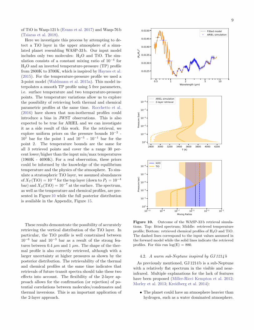
4.1. An ultra Hot-Jupiter inspired by WASP-33 b
Current analyses of ground and space-based obser-
vations of WASP-33 b suggest extreme temperatures
reaching 3800 K and a possible thermal inversion in the
atmosphere (Haynes et al. 2015; Nugroho et al. 2017).
TiO or VO, which are strong absorbers at short wave-
lengths, could very efficiently capture high-energy stel-
lar photons at the top of the atmosphere and cause the
inversion (Fortney et al. 2008; Spiegel et al. 2009). In
parallel, other observations have suggested the presence
9
of TiO in Wasp-121 b (Evans et al. 2017) and Wasp-76 b
(Tsiaras et al. 2018).
Here we investigate this process by attempting to de-
tect a TiO layer in the upper atmosphere of a simu-
lated planet resembling WASP-33 b. Our input model
includes only two molecules: H2O and TiO. The sim-
ulation consists of a constant mixing ratio of 10−4 for
H2O and an inverted temperature-pressure (TP) profile
from 2800K to 3700K, which is inspired by Haynes et al.
(2015). For the temperature-pressure profile we used a
3-point model (Waldmann et al. 2015a). This model in-
terpolates a smooth TP profile using 5 free parameters,
i.e. surface temperature and two temperature-pressure
points. The temperature variations allow us to explore
the possibility of retrieving both thermal and chemical
parametric profiles at the same time. Rocchetto et al.
(2016) have shown that non-isothermal profiles could
introduce a bias in JWST observations. This is also
expected to be true for ARIEL and we can investigate
it as a side result of this work. For the retrieval, we
explore uniform priors on the pressure bounds 10−2 -
101 bar for the point 1 and 10−5 - 10−1 bar for the
point 2. The temperature bounds are the same for
all 3 retrieved points and cover the a range 30 per-
cent lower/higher than the input min/max temperatures
(1960K - 4690K). For a real observation, these priors
could be informed by the knowledge of the equilibrium
temperature and the physics of the atmosphere. To sim-
ulate a stratospheric TiO layer, we assumed abundances
ofXT (TiO) = 10−4 for the top layer (down to PI = 10−4
bar) andXS(TiO) = 10−7 at the surface. The spectrum,
as well as the temperature and chemical profiles, are pre-
sented in Figure 10 while the full posterior distribution
is available in the Appendix, Figure 15.
These results demonstrate the possibility of accurately
retrieving the vertical distribution of the TiO layer. In
particular, the TiO profile is well constrained between
10−6 bar and 10−3 bar as a result of the strong fea-
tures between 0.4 µm and 1 µm. The shape of the ther-
mal profile is also correctly retrieved, although with a
larger uncertainty at higher pressures as shown by the
posterior distribution. The retrievability of the thermal
and chemical profiles at the same time indicates that
retrievals of future transit spectra should take these two
effects into account. The flexibility of the 2-layer ap-
proach allows for the confirmation (or rejection) of po-
tential correlations between molecules/condensates and
thermal inversions. This is an important application of
the 2-layer approach.
0.5 1 2 5 10Wavelength ( m)
0.0125
0.0130
0.0135
0.0140
0.0145
0.0150
(Rp/R
s)2
Fitted modelARIEL simulation
2800 3000 3200 3400 3600 3800 4000 4200T (K)
10 9
10 7
10 5
10 3
10 1
101Pr
essu
re (b
ar)
ARIEL simulation2-layer retrieval
10 11 10 9 10 7 10 5 10 3 10 1
Mixing Ratios
10 9
10 7
10 5
10 3
10 1
101
Pres
sure
bar
)
H2OTIO
Figure 10. Outcome of the WASP-33 b retrieval simula-tions. Top: fitted spectrum; Middle: retrieved temperatureprofile; Bottom: retrieved chemical profiles of H2O and TiO.The dashed lines correspond to the input values assumed inthe forward model while the solid lines indicate the retrievedprofiles. For this run log(E) = 880.
4.2. A warm sub-Neptune inspired by GJ 1214 b
As previously mentioned, GJ 1214 b is a sub-Neptune
with a relatively flat spectrum in the visible and near-
infrared. Multiple explanations for the lack of features
have been proposed (Miller-Ricci Kempton et al. 2012;
Morley et al. 2013; Kreidberg et al. 2014):
• The planet could have an atmosphere heavier than
hydrogen, such as a water dominated atmosphere.
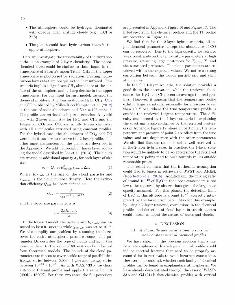
10
• The atmosphere could be hydrogen dominated
with opaque, high altitude clouds (e.g. KCl or
ZnS).
• The planet could have hydrocarbon hazes in the
upper atmosphere.
Here we investigate the retrievability of the third sce-
nario as an example of 2-layer chemistry. The photo-
chemical hazes could be similar to those found in the
atmosphere of Saturn’s moon Titan. CH4 in the upper
atmosphere is photolysed by radiation, creating hydro-
carbon hazes that are opaque in the near infrared. This
scenario implies a significant CH4 abundance at the sur-
face of the atmosphere and a sharp decline in the upper
atmosphere. For our input forward model, we used the
chemical profiles of the four molecules H2O, CH4, CO2
and CO published by Miller-Ricci Kempton et al. (2012)
in the case of solar abundance and Kzz = 106 cm2s−1.
The profiles are retrieved using two scenarios: A hybrid
one with 2-layer chemistry for H2O and CH4 and the
1-layer for CO2 and CO; and a fully 1-layer chemistry
with all 4 molecules retrieved using constant profiles.
For the hybrid case, the abundances of CO2 and CO
were indeed too low to retrieve the 2-layer profile. The
other input parameters for the planet are described in
the Appendix. We add hydrocarbon hazes layer adopt-
ing the model described in Lee et al. (2013). The clouds
are treated as additional opacity σc for each layer of size
∆z:
σc = QextπR2cloudsχclouds∆z. (1)
Where Rclouds is the size of the cloud particles and
χclouds is the cloud number density. Here the extinc-
tion efficiency Qext has been defined as:
Qext =5
Q0x−4 + x0.2, (2)
and the cloud size parameter x is:
x =2πRclouds
λ. (3)
In the forward model, the particle size Rclouds was as-
sumed to be 0.01 microns while χclouds was set to 10−6.
We also simplify our problem by assuming the hazes
cover the entire atmospheric pressure range. The pa-
rameter Q0 describes the type of clouds and is, in this
example, fixed to the value of 80 as it can be informed
from theoretical models. The bounds of the cloud pa-
rameters are chosen to cover a wide range of possibilities:
Rclouds varies between 0.003 - 1 µm and χclouds varies
between 10−15 - 10−3. As with WASP-33 b, we chose
a 3-point thermal profile and apply the same bounds
(490K - 1690K). For these two cases, the full posteriors
are presented in Appendix Figure 16 and Figure 17. The
fitted spectrum, the chemical profiles and the TP profile
are presented in Figure 11.
We find that for the 2-layer hybrid scenario, all in-
put chemical parameters except the abundance of CO
can be recovered. Due to the high opacity, we retrieve
weak constraints on the temperature parameters at high
pressure, returning large posteriors for Tsurf , T1 and
the associated pressures. The cloud parameters are re-
trieved within the expected values. We notice a strong
correlation between the clouds particle size and their
abundances.
In the full 1-layer scenario, the solution provides a
good fit to the observation, while the retrieved abun-
dances for H2O and CH4 seem to average the real pro-
files. However, it appears that the temperature profile
exhibit large variations, especially for pressures lower
than 10−2 bar, where the true temperature profile is
outside the retrieved 1-sigma temperature. The diffi-
culty encountered by the 1-layer scenario in explaining
the spectrum is also confirmed by the retrieved posteri-
ors in Appendix Figure 17 where, in particular, the tem-
perature and pressure of point 2 are offset from the true
values and are degenerate with the other parameters.
We also find that the radius is not as well retrieved as
in the 2-layer hybrid case. In practice, the 1-layer solu-
tion would be unlikely to be accepted since the retrieved
temperature points tend to push towards values outside
reasonable priors.
This result confirms that the isothermal assumption
could lead to biases in retrievals of JWST and ARIEL
(Rocchetto et al. 2016). Additionally, the mixing ratio
of around 10−10 of H2O in the upper atmosphere is too
low to be captured by observations given the large haze
opacity assumed. For this planet, the detection limit
of H2O at this altitude is around 10−5, correctly inter-
preted by the large error bars. Also for this example,
by using a 2-layer retrieval, correlations in the chemical
profiles and detection of cloud layers in transit spectra
could inform us about the nature of hazes and clouds.
5. DISCUSSION
5.1. A physically motivated reason to consider
non-constant vertical chemical profiles
We have shown in the previous sections that simu-
lated atmospheres with a 2-layer chemical profile would
induce spectral features that need to be properly ac-
counted for in retrievals to avoid incorrect conclusions.
However, one could ask whether such family of chemical
profiles can be found in exoplanetary atmospheres. We
have already demonstrated through the cases of WASP-
33 b and GJ 1214 b that chemical profiles with vertical
11
0.5 1 2 5 10Wavelength ( m)
0.022
0.024
0.026
0.028
0.030
0.032
0.034
(Rp/R
s)2
Fitted modelARIEL simulation
0.5 1 2 5 10Wavelength ( m)
0.022
0.024
0.026
0.028
0.030
0.032
0.034
(Rp/R
s)2
Fitted modelARIEL simulation
700 800 900 1000 1100 1200 1300 1400T (K)
10 9
10 7
10 5
10 3
10 1
101
Pres
sure
(bar
)
ARIEL simulation2-layer retrieval
600 800 1000 1200 1400 1600T (K)
10 9
10 7
10 5
10 3
10 1
101
Pres
sure
(bar
)
ARIEL simulation2-layer retrieval
10 11 10 9 10 7 10 5 10 3 10 1
Mixing Ratios
10 9
10 7
10 5
10 3
10 1
101
Pres
sure
bar
)
H2OCH4CO2CO
10 11 10 9 10 7 10 5 10 3 10 1
Mixing Ratios
10 9
10 7
10 5
10 3
10 1
101
Pres
sure
bar
)
H2OCH4CO2CO
Figure 11. Results of the retrieval for a planet like GJ 1214 b. Left: 2-layer profile for H2O and CH4, while CO2 and CO useconstant profiles. Right: all molecules are retrieved with constant (1-layer profile) chemistry. Top rows: fitted spectra, middlerows: temperature profiles and bottom rows: chemical profiles of H2O, CH4 and CO2 and CO. For the temperature and thechemical profiles, the dotted lines correspond to the input values. For the 2-layer run we obtain log(E) = 736, while for the1-layer run we get log(E) = 691 (∆log(E) = 45).
discontinuities could be important if clouds and hazes
are present in the atmosphere.
Additionally, chemical simulations by Venot et al.
(2012) suggest at least two typical behaviours for chem-
ical profiles in exoplanetary atmospheres of the type
HD 209458b. Some molecules of interest, such as H2O
and CO, are predicted to have a constant mixing ratios
as a function of pressure. Others, like NH3 or CH4, are
expected to vary with altitude. In the deep atmosphere
(generally pressures higher than 1 bar / 105 Pa) chemical
reactions are close to their thermochemical equilibrium
values. In the higher part of the atmosphere (∼ 10−4 bar
/ 10 Pa) photo-chemistry and disequilibrium processes
may modify the overall mix by dissociation and creation
of atomic species and new molecules. In addition, Moses
et al. (2013) investigated the composition of Hot Nep-
tunes like GJ 436 b with a wide range of metallicities
and the resulting chemical profiles demonstrated com-
plex behaviours. This highlights the need for adapted
retrieval techniques. These disequilibrium processes are
12
expected to be more prominent and important in colder
atmospheres (Tinetti et al. 2018).
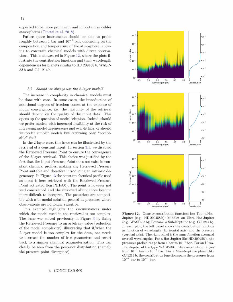
Future space instruments should be able to probe
roughly between 1 bar and 10−5 bar, depending on the
composition and temperature of the atmosphere, allow-
ing to constrain chemical models with direct observa-
tions. This is showcased in Figure 12, where the plots il-
lustrate the contribution functions and their wavelength
dependencies for planets similar to HD 209458 b, WASP-
33 b and GJ 1214 b.
5.2. Should we always use the 2-layer model?
The increase in complexity in chemical models must
be done with care. In some cases, the introduction of
additional degrees of freedom comes at the expense of
model convergence, i.e: the flexibility of the retrieval
should depend on the quality of the input data. This
opens up the question of model selection. Indeed, should
we prefer models with increased flexibility at the risk of
increasing model degeneracies and over-fitting, or should
we prefer simpler models but returning only “accept-
able” fits?
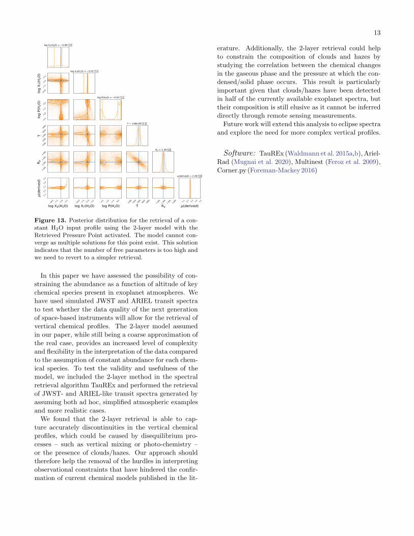
In the 2-layer case, this issue can be illustrated by the
retrieval of a constant input. In section 3.1, we disabled
the Retrieved Pressure Point to ensure the convergence
of the 2-layer retrieval. This choice was justified by the
fact that the Input Pressure Point does not exist in con-
stant chemical profiles, making any Retrieved Pressure
Point suitable and therefore introducing an intrinsic de-
generacy. In Figure 13 the constant chemical profile used
as input is here retrieved with the Retrieved Pressure
Point activated (log P(H2O)). The point is however not
well constrained and the retrieved abundances become
more difficult to interpret. The posteriors are compati-
ble with a bi-modal solution peaked at pressures where
observations are no longer sensitive.
This example highlights the circumstances under
which the model used in the retrieval is too complex.
The issue was solved previously in Figure 3 by fixing
the Retrieved Pressure to an arbitrary value (reduction
of the model complexity), illustrating that if/when the
2-layer model is too complex for the data, one needs
to decrease the number of free parameters and revert
back to a simpler chemical parameterisation. This can
clearly be seen from the posterior distribution (namely
the pressure point divergence).
6. CONCLUSIONS
0.5 0.9 1.6 2.8 4.9 8.6Wavelength ( m)
101
10 1
10 3
10 5
10 7
10 9
Pres
sure
(Bar
)
0 1Contribution
10 9
10 7
10 5
10 3
10 1
101
0.5 0.9 1.6 2.8 4.9 8.6Wavelength ( m)
101
10 1
10 3
10 5
10 7
10 9
Pres
sure
(Bar
)
0 1Contribution
10 9
10 7
10 5
10 3
10 1
101
0.5 0.9 1.6 2.8 4.9 8.6Wavelength ( m)
101
10 1
10 3
10 5
10 7
10 9
Pres
sure
(Bar
)
0 1Contribution
10 9
10 7
10 5
10 3
10 1
101
Figure 12. Opacity contribution functions for: Top: a Hot-Jupiter (e.g. HD 209458 b); Middle: an Ultra Hot-Jupiter(e.g. WASP-33 b); Bottom: a Sub-Neptune (e.g. GJ 1214 b).In each plot, the left panel shows the contribution functionas function of wavelength (horizontal axis) and the pressure(vertical axis). The right panel is the same function averagedover all wavelengths. For a Hot Jupiter like HD 209458 b, thepressures probed range from 1 bar to 10−4 bar. For an Ultra-Hot Jupiter of the type WASP-33 b, the contribution rangesfrom 10−1 bar to 10−7 bar. For a Mini-Neptune planet likeGJ 1214 b, the contribution function spans the pressures from10−1 bar to 10−6 bar.
13
log XS(H2O) = 5.06+0.593.47
10.0
7.55.02.5
log
X T(H
2O) log XT(H2O) = 5.01+0.14
1.91
4.5
3.0
1.5
0.0
log
P(H 2
O)
log P(H2O) = 0.01+0.734.49
1200
1350
1500
1650
1800
T
T = 1496.99+47.8451.82
1.385
1.390
1.395
1.400
R p
Rp = 1.39+0.000.00
10.0 7.5 5.0 2.5
log XS(H2O)
2.12.22.32.42.5
(der
ived
)
10.0 7.5 5.0 2.5
log XT(H2O)4.5 3.0 1.5 0.0
log P(H2O)12
0013
5015
0016
5018
00
T1.3
851.3
901.3
951.4
00
Rp
2.1 2.2 2.3 2.4 2.5
(derived)
(derived) = 2.26+0.000.00
Figure 13. Posterior distribution for the retrieval of a con-stant H2O input profile using the 2-layer model with theRetrieved Pressure Point activated. The model cannot con-verge as multiple solutions for this point exist. This solutionindicates that the number of free parameters is too high andwe need to revert to a simpler retrieval.
In this paper we have assessed the possibility of con-
straining the abundance as a function of altitude of key
chemical species present in exoplanet atmospheres. We
have used simulated JWST and ARIEL transit spectra
to test whether the data quality of the next generation
of space-based instruments will allow for the retrieval of
vertical chemical profiles. The 2-layer model assumed
in our paper, while still being a coarse approximation of
the real case, provides an increased level of complexity
and flexibility in the interpretation of the data compared
to the assumption of constant abundance for each chem-
ical species. To test the validity and usefulness of the
model, we included the 2-layer method in the spectral
retrieval algorithm TauREx and performed the retrieval
of JWST- and ARIEL-like transit spectra generated by
assuming both ad hoc, simplified atmospheric examples
and more realistic cases.
We found that the 2-layer retrieval is able to cap-
ture accurately discontinuities in the vertical chemical
profiles, which could be caused by disequilibrium pro-
cesses – such as vertical mixing or photo-chemistry –
or the presence of clouds/hazes. Our approach should
therefore help the removal of the hurdles in interpreting
observational constraints that have hindered the confir-
mation of current chemical models published in the lit-
erature. Additionally, the 2-layer retrieval could help
to constrain the composition of clouds and hazes by
studying the correlation between the chemical changes
in the gaseous phase and the pressure at which the con-
densed/solid phase occurs. This result is particularly
important given that clouds/hazes have been detected
in half of the currently available exoplanet spectra, but
their composition is still elusive as it cannot be inferred
directly through remote sensing measurements.
Future work will extend this analysis to eclipse spectra
and explore the need for more complex vertical profiles.
Software: TauREx (Waldmann et al. 2015a,b), Ariel-
Rad (Mugnai et al. 2020), Multinest (Feroz et al. 2009),
Corner.py (Foreman-Mackey 2016)
14
Acknowledgements
This project has received funding from the European
Research Council (ERC) under the European Union’s
Horizon 2020 research and innovation programme (grant
agreement No 758892, ExoAI), under the European
Union’s Seventh Framework Programme (FP7/2007-
2013)/ ERC grant agreement numbers 617119 (Exo-
Lights) and the European Union’s Horizon 2020 COM-
PET programme (grant agreement No 776403, Exo-
plANETS A). Furthermore, we acknowledge funding by
the Science and Technology Funding Council (STFC)
grants: ST/K502406/1, ST/P000282/1, ST/P002153/1,
ST/T001836/1 and ST/S002634/1.
REFERENCES
Abel, M., Frommhold, L., Li, X., & Hunt, K. L. 2011, The
Journal of Physical Chemistry A, 115, 6805
—. 2012, The Journal of chemical physics, 136, 044319
Agundez, M., Parmentier, V., Venot, O., Hersant, F., &
Selsis, F. 2014, A&A, 564, A73
Barton, E. J., Hill, C., Yurchenko, S. N., et al. 2017,
Journal of Quantitative Spectroscopy and Radiative
Transfer, 187, 453
Bean, J. L., Stevenson, K. B., Batalha, N. M., et al. 2018,
Publications of the Astronomical Society of the Pacific,
130, 114402
Brandl, B. R., Absil, O., Agocs, T., et al. 2018, in Society
of Photo-Optical Instrumentation Engineers (SPIE)
Conference Series, Vol. 10702, Ground-based and
Airborne Instrumentation for Astronomy VII, 107021U
Cox, A. N. 2015, Allen’s astrophysical quantities (Springer)
Cubillos, P., Blecic, J., Harrington, J., et al. 2016, BART:
Bayesian Atmospheric Radiative Transfer fitting code,
Astrophysics Source Code Library, , , ascl:1608.004
Edwards, B., Mugnai, L., Tinetti, G., Pascale, E., & Sarkar,
S. 2019a, AJ, 157, 242
Edwards, B., Rice, M., Zingales, T., et al. 2019b,
Experimental Astronomy, 47, 29
Evans, T. M., Sing, D. K., Kataria, T., et al. 2017, Nature,
548, 58
Feng, Y. K., Robinson, T. D., Fortney, J. J., et al. 2018,
AJ, 155, 200
Feroz, F., Hobson, M. P., & Bridges, M. 2009, MNRAS,
398, 1601
Fletcher, L. N., Gustafsson, M., & Orton, G. S. 2018, The
Astrophysical Journal Supplement Series, 235, 24
Foreman-Mackey, D. 2016, The Journal of Open Source
Software, 1, 24. https://doi.org/10.21105/joss.00024
Fortney, J. J., Lodders, K., Marley, M. S., & Freedman,
R. S. 2008, ApJ, 678, 1419
Gandhi, S., & Madhusudhan, N. 2018, MNRAS, 474, 271
Gordon, I., Rothman, L. S., Wilzewski, J. S., et al. 2016, in
AAS/Division for Planetary Sciences Meeting Abstracts,
Vol. 48, AAS/Division for Planetary Sciences Meeting
Abstracts #48, 421.13
Goyal, J. M., Mayne, N., Sing, D. K., et al. 2018, MNRAS,
474, 5158
Guillot, T. 2010, A&A, 520, A27
Harpsøe, K. B. W., Hardis, S., Hinse, T. C., et al. 2013,
A&A, 549, A10
Haynes, K., Mandell, A. M., Madhusudhan, N., Deming,
D., & Knutson, H. 2015, The Astrophysical Journal, 806,
146. http://stacks.iop.org/0004-637X/806/i=2/a=146
Heng, K., Mendonca, J. M., & Lee, J.-M. 2014, The
Astrophysical Journal Supplement Series, 215, 4
Hill, C., Yurchenko, S. N., & Tennyson, J. 2013, Icarus,
226, 1673
Irwin, P. G. J., Teanby, N. A., de Kok, R., et al. 2008,
JQSRT, 109, 1136
Jeffreys, H. 1998, The theory of probability (OUP Oxford)
Kass, R. E., & Raftery, A. E. 1995, Journal of the american
statistical association, 90, 773
Kreidberg, L., Bean, J. L., Desert, J.-M., et al. 2014,
Nature, 505, 69
Lavie, B., Mendonca, J. M., Mordasini, C., et al. 2017, AJ,
154, 91
Lee, J.-M., Heng, K., & Irwin, P. G. J. 2013, The
Astrophysical Journal, 778, 97. https:
//doi.org/10.1088%2F0004-637x%2F778%2F2%2F97
Li, G., Gordon, I. E., Rothman, L. S., et al. 2015, The
Astrophysical Journal Supplement Series, 216, 15
Line, M. R., Wolf, A. S., Zhang, X., et al. 2013, ApJ, 775,
137
MacDonald, R. J., & Madhusudhan, N. 2017, MNRAS, 469,
1979
Madhusudhan, N., & Seager, S. 2009, ApJ, 707, 24
Malik, M., Grosheintz, L., Mendonca, J. M., et al. 2017,
AJ, 153, 56
Miller-Ricci Kempton, E., Zahnle, K., & Fortney, J. J.
2012, ApJ, 745, 3
Morley, C. V., Fortney, J. J., Kempton, E. M.-R., et al.
2013, The Astrophysical Journal, 775, 33. https:
//doi.org/10.1088%2F0004-637x%2F775%2F1%2F33
Moses, J. I., Line, M. R., Visscher, C., et al. 2013, ApJ,
777, 34
15
Mugnai, L. V., Pascale, E., Edwards, B., Papageorgiou, A.,
& Sarkar, S. 2020, arXiv e-prints, arXiv:2009.07824
Nugroho, S. K., Kawahara, H., Masuda, K., et al. 2017, AJ,
154, 221
Pinhas, A., Madhusudhan, N., Gandhi, S., & MacDonald,
R. 2019, Monthly Notices of the Royal Astronomical
Society, 482, 1485.
http://dx.doi.org/10.1093/mnras/sty2544
Polyansky, O. L., Kyuberis, A. A., Zobov, N. F., et al.
2018, Monthly Notices of the Royal Astronomical
Society, 480, 2597
Rocchetto, M., Waldmann, I. P., Venot, O., Lagage, P. O.,
& Tinetti, G. 2016, ApJ, 833, 120
Rothman, L., Gordon, I., Barber, R., et al. 2010, Journal of
Quantitative Spectroscopy and Radiative Transfer, 111,
2139
Rothman, L. S., & Gordon, I. E. 2014, in 13th International
HITRAN Conference, June 2014, Cambridge,
Massachusetts, USA
Schwenke, D. W. 1998, Faraday Discussions, 109, 321
Spiegel, D. S., Silverio, K., & Burrows, A. 2009, ApJ, 699,
1487
Stassun, K. G., Collins, K. A., & Gaudi, B. S. 2017, AJ,
153, 136
Tennyson, J., Yurchenko, S. N., Al-Refaie, A. F., et al. 2016,
Journal of Molecular Spectroscopy, 327, 73 , new Visions
of Spectroscopic Databases, Volume II. http://www.
sciencedirect.com/science/article/pii/S0022285216300807
Terrile, R. J., Fink, W., Huntsberger, T., et al. 2005, in
Bulletin of the American Astronomical Society, Vol. 37,
AAS/Division for Planetary Sciences Meeting Abstracts
#37, 1566
Tinetti, G., Drossart, P., Eccleston, P., et al. 2018,
Experimental Astronomy, doi:10.1007/s10686-018-9598-x
Tsiaras, A., Waldmann, I. P., Zingales, T., et al. 2018, AJ,
155, 156
Venot, O., Hebrard, E., Agundez, M., et al. 2012, A&A,
546, A43
Waldmann, I. P., Rocchetto, M., Tinetti, G., et al. 2015a,
ApJ, 813, 13
Waldmann, I. P., Tinetti, G., Rocchetto, M., et al. 2015b,
ApJ, 802, 107
Yurchenko, S. N., & Tennyson, J. 2014, Monthly Notices of
the Royal Astronomical Society, 440, 1649

16
APPENDIX
PLANET’S PARAMETERS USED FOR THE FORWARD MODELS
Parameters used in our forward models for the 3 types of planets: a hot-Jupiter type HD 209458 b (Stassun et al.
(2017)), an Ultra hot-Jupiter type WASP-33 b (Stassun et al. (2017)) and a Sub Neptune Type GJ 1214 b (Harpsøe
et al. (2013)):
Parameters Hot Jupiter Ultra Hot Jupiter Sub Neptune
Rs(Rsun) 1.19 1.55 0.216
Ts(K) 6091 7308 3026
Rp(RJupiter) 1.39 1.6 0.254
Mp(MJupiter) 0.73 1.17 0.0197
POSTERIORS OF RETRIEVALS FOR A PLANET WITH AN INVERTED H2O CHEMICAL PROFILE USING
CONSTANT AND 2-LAYER CHEMICAL MODELS
log XS(H2O) = 9.09+2.061.99
3.63.22.82.42.0
log
X T(H
2O) log XT(H2O) = 3.00+0.13
0.14
2.82.42.01.61.2
log
P(H 2
O)
log P(H2O) = 2.07+0.160.18
1380
1440
1500
1560
1620
T
T = 1500.34+25.7725.97
1.385
1.390
1.395
1.400
R p
Rp = 1.39+0.000.00
10.0 7.5 5.0 2.5
log XS(H2O)
2.12.22.32.42.5
(der
ived
)
3.6 3.2 2.8 2.4 2.0
log XT(H2O)2.8 2.4 2.0 1.6 1.2
log P(H2O)13
8014
4015
0015
6016
20
T1.3
851.3
901.3
951.4
00
Rp
2.1 2.2 2.3 2.4 2.5
(derived)
(derived) = 2.26+0.000.00
log X(H2O) = 4.74+0.060.06
1400
1600
1800
2000
2200
T
T = 2102.09+38.7839.95
1.370
1.375
1.380
1.385
1.390
R p
Rp = 1.38+0.000.00
4.95
4.80
4.65
4.50
log X(H2O)
2.12.22.32.42.5
(der
ived
)
1400
1600
1800
2000
2200
T1.3
701.3
751.3
801.3
851.3
90
Rp
2.1 2.2 2.3 2.4 2.5
(derived)
(derived) = 2.26+0.000.00
Figure 14. Posteriors of the 2-layer retrieval (left) and the constant retrieval (right) for a simulated ARIEL observation of aplanet with an inverted H2O profile. The top layer contains XT (H2O) = 10−3 for pressures lower than PI(H2O) = 10−2 barand the surface layer is depleted with a mixing ratio of only XS(H2O) = 10−10.
17
POSTERIORS DISTRIBUTION FOR THE RETRIEVAL OF WASP-33 B
log H2O = 4.53+1.050.92
10.0
7.55.02.5
log
X S(T
iO)
log XS(TiO) = 7.85+1.352.24
8
6
4
2
log
X T(T
iO)
log XT(TiO) = 4.53+1.100.93
4.5
3.0
1.5
0.0
log
P(Ti
O)
log P(TiO) = 3.41+1.041.16
2400
3000
3600
4200
T sur
f
Tsurf = 3523.38+680.55876.20
2400
3000
3600
4200
T 1
T1 = 3281.27+499.02738.05
2400
3000
3600
4200
T 2
T2 = 3692.71+289.47186.95
1.81.20.60.00.6
P 1
P1 = 0.47+0.880.93
4.84.03.22.41.6
P 2
P2 = 3.25+1.331.07
1.44
1.50
1.56
1.62
1.68
R p
Rp = 1.61+0.030.04
8 6 4 2
log H2O
2.12.22.32.42.5
(der
ived
)
10.0 7.5 5.0 2.5
log XS(TiO)8 6 4 2
log XT(TiO)4.5 3.0 1.5 0.0
log P(TiO)24
0030
0036
0042
00
Tsurf24
0030
0036
0042
00
T124
0030
0036
0042
00
T2
1.8 1.2 0.6 0.0 0.6
P1
4.8 4.0 3.2 2.4 1.6
P21.4
41.5
01.5
61.6
21.6
8
Rp
2.1 2.2 2.3 2.4 2.5
(derived)
(derived) = 2.26+0.000.00
Figure 15. Posteriors distribution for the retrieval of WASP-33 b. The planet presents constant H2O abundance and a TiO2-layer profile with a large abundance in the upper atmosphere.
18
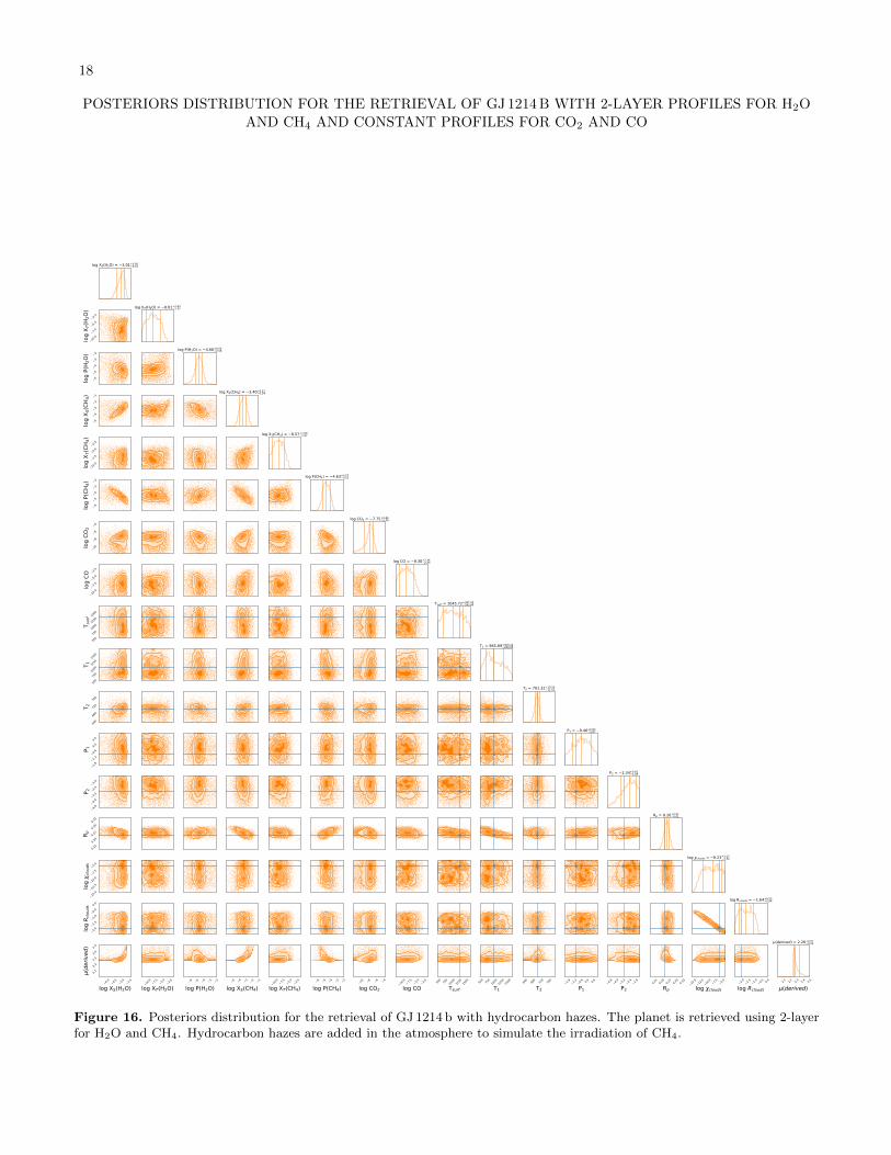
POSTERIORS DISTRIBUTION FOR THE RETRIEVAL OF GJ 1214 B WITH 2-LAYER PROFILES FOR H2O
AND CH4 AND CONSTANT PROFILES FOR CO2 AND CO
log XS(H2O) = 3.01+0.660.91
10.0
7.55.02.5
log
X T(H
2O) log XT(H2O) = 8.01+2.43
2.42
6
5
4
3
2
log
P(H 2
O)
log P(H2O) = 4.66+0.530.58
5
4
3
2
1
log
X S(C
H 4) log XS(CH4) = 3.40+0.51
0.54
10.0
7.55.02.5
log
X T(C
H 4) log XT(CH4) = 8.57+1.89
1.97
6
5
4
3
2
log
P(CH
4)
log P(CH4) = 4.63+0.570.55
10
8
6
4
log
CO2
log CO2 = 7.75+0.821.39
10.0
7.55.02.5
log
CO
log CO = 8.30+2.342.33
500
750
1000
1250
1500
T sur
f
Tsurf = 1045.72+387.95343.49
500
750
1000
1250
1500
T 1
T1 = 965.89+400.22284.68
640
680
720
760
T 2
T2 = 701.32+10.5011.62
1.81.20.60.00.6
P 1
P1 = 0.46+0.830.87
4.84.03.22.41.6
P 2
P2 = 2.34+0.811.09
0.21
0.24
0.27
0.30
0.33
R p
Rp = 0.26+0.010.01
15.0
12.5
10.0
7.55.0
log
clou
ds
log clouds = 8.23+3.273.34
2.01.51.00.50.0
log
R clo
uds
log Rclouds = 1.64+0.550.54
6.0 4.5 3.0 1.5
log XS(H2O)
2.12.22.32.42.5
(der
ived
)
10.0 7.5 5.0 2.5
log XT(H2O)6 5 4 3 2
log P(H2O)5 4 3 2 1
log XS(CH4)10
.0 7.5 5.0 2.5
log XT(CH4)6 5 4 3 2
log P(CH4)10 8 6 4
log CO210
.0 7.5 5.0 2.5
log CO50
075
010
0012
5015
00
Tsurf
500
750
1000
1250
1500
T164
068
072
076
0
T21.8 1.2 0.6 0.0 0.6
P14.8 4.0 3.2 2.4 1.6
P20.2
10.2
40.2
70.3
00.3
3
Rp15
.012
.510
.0 7.5 5.0
log clouds
2.0 1.5 1.0 0.5 0.0
log Rclouds
2.1 2.2 2.3 2.4 2.5
(derived)
(derived) = 2.28+0.070.02
Figure 16. Posteriors distribution for the retrieval of GJ 1214 b with hydrocarbon hazes. The planet is retrieved using 2-layerfor H2O and CH4. Hydrocarbon hazes are added in the atmosphere to simulate the irradiation of CH4.
19
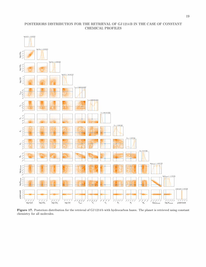
POSTERIORS DISTRIBUTION FOR THE RETRIEVAL OF GJ 1214 B IN THE CASE OF CONSTANT
CHEMICAL PROFILES
log H2O = 5.53+0.220.22
5.75.45.14.8
log
CH4
log CH4 = 5.35+0.130.13
10.5
9.07.56.0
log
CO2
log CO2 = 8.94+0.420.90
10
8
6
4
log
CO
log CO = 10.24+1.381.12
500
750
1000
1250
1500
T sur
f
Tsurf = 1360.56+224.69321.47
500
750
1000
1250
1500
T 1
T1 = 1269.90+291.85412.79
640
680
720
760
T 2
T2 = 632.32+18.5870.58
1.81.20.60.00.6
P 1
P1 = 0.93+1.000.60
4.84.03.22.41.6
P 2
P2 = 1.87+0.532.06
0.24
0.26
0.28
0.30
R p
Rp = 0.27+0.010.01
15.0
12.5
10.0
7.55.0
log
clou
ds
log clouds = 8.97+3.003.12
2.01.51.00.50.0
log
R clo
uds
log Rclouds = 1.75+0.520.50
6.6 6.0 5.4 4.8
log H2O
2.12.22.32.42.5
(der
ived
)
5.7 5.4 5.1 4.8
log CH410
.5 9.0 7.5 6.0
log CO2
10 8 6 4
log CO50
075
010
0012
5015
00
Tsurf
500
750
1000
1250
1500
T164
068
072
076
0
T21.8 1.2 0.6 0.0 0.6
P14.8 4.0 3.2 2.4 1.6
P20.2
40.2
60.2
80.3
0
Rp15
.012
.510
.0 7.5 5.0
log clouds
2.0 1.5 1.0 0.5 0.0
log Rclouds
2.1 2.2 2.3 2.4 2.5
(derived)
(derived) = 2.26+0.000.00
Figure 17. Posteriors distribution for the retrieval of GJ 1214 b with hydrocarbon hazes. The planet is retrieved using constantchemistry for all molecules.