quadrotor team modeling and control for dlo transportation · quadrotor team modeling and control...
TRANSCRIPT
Quadrotor Team Modeling andControl for DLO Transportation
By
Julián Estévez Sanz
Submitted to the department of Computer Science and Artificial Intelligence in partialfulfillment of the requirements for the degree of Doctor of Philosophy
PhD Advisor:
Prof. Manuel Graña Romayat The University of the Basque Country (UPV/EHU)
Euskal Herriko UnibertsitateaUniversidad del País VascoDonostia - San Sebastián
2016

AUTORIZACION DEL/LA DIRECTOR/A DE TESIS
PARA SU PRESENTACION
Dr. MANUEL M. GRAÑA ROMAY con N.I.F. 15932620Z como Director de la Tesis
Doctoral: Quadrotor Modeling and Control for DLO Transportation realizada en el
Programa de Doctorado en Ingeniería Informática por el Doctorando D. JULIÁN
ESTÉVEZ SANZ, autorizo la presentación de la citada Tesis Doctoral, dado que
reúne las condiciones necesarias para su defensa.
En DONOSTIA a 16 de mayo de 2016
EL DIRECTOR DE LA TESIS
Fdo.:

CONFORMIDAD DEL DEPARTAMENTO
El Consejo del Departamento de CIENCIAS DE LA COMPUTACIÓN E INTELIGENCIA
ARTIFICIAL en reunión celebrada el día ___ de ____________ de 201__ ha acordado
dar la conformidad a la admisión a trámite de presentación de la Tesis Doctoral
titulada: Quadrotor Modeling and Control for DLO Transportation dirigida por el Dr.
MANUEL M. GRAÑA ROMAY y presentada por Don JULIÁN ESTÉVEZ SANZ ante
este Departamento.
En DONOSTIA a ___ de ____________ de 201__
VºBº DIRECTOR/A DEL DEPARTAMENTO SECRETARIO/A DEL DEPARTAMENTO
Fdo.:____________________________ Fdo.:____________________________

AUTORIZACIÓN DE LA COMISIÓN ACADÉMICA DEL PROGRAMA DE
DOCTORADO
La Comisión Académica del Programa de Doctorado en Ingeniería
Informática en reunión celebrada el día ____ de ___________ de 201___, ha
acordado dar la conformidad a la presentación de la Tesis Doctoral
titulada: Quadrotor Modeling and Control for DLO Transportation dirigida
por el Dr. MANUEL M. GRAÑA ROMAY y presentada por D. JULIÁN ESTÉVEZ
SANZ adscrito al Departamento CIENCIAS DE LA COMPUTACIÓN E
INTELIGENCIA ARTIFICIAL
En DONOSTIA a de de
EL MIEMBRO DE LA COMISIÓN ACADÉMICA RESPONSABLE DEL
PROGRAMA DE DOCTORADO
Fdo.: _____________________________________

ACTA DE GRADO DE DOCTOR O DOCTORA ACTA DE DEFENSA DE TESIS DOCTORAL
DOCTORANDO/A D. Julián Estévez Sanz
TITULO DE LA TESIS: Quadrotor Modeling and Control for DLO Transportation
El Tribunal designado por la Comisión de Postgrado de la UPV/EHU para calificar la Tesis
Doctoral arriba indicada y reunido en el día de la fecha, una vez efectuada la defensa por el/la
doctorando/a y contestadas las objeciones y/o sugerencias que se le han formulado, ha
otorgado por___________________ la calificación de: unanimidad ó mayoría
SOBRESALIENTE / NOTABLE / APROBADO / NO APTO
Idioma/s de defensa (en caso de más de un idioma, especificar porcentaje defendido en cada
idioma):
Castellano _______________________________________________________________
Euskera _______________________________________________________________
Otros Idiomas (especificar cuál/cuales y porcentaje) ______________________________
En a de de
EL/LA PRESIDENTE/A, EL/LA SECRETARIO/A,
Fdo.: Fdo.:
Dr/a: ____________________ Dr/a: ______________________
VOCAL 1º, VOCAL 2º, VOCAL 3º,
Fdo.: Fdo.: Fdo.:
Dr/a: Dr/a: Dr/a:
EL/LA DOCTORANDO/A,
Fdo.: _____________________

Acknowledgments
Third time lucky, and it is sure that would have been not possible without Prof.Manuel Graña. During this time, both of us had to learn to rely on each other andovercome all the inquisitive reviewers. Thanks specially for getting me enjoy thisjob and research field.
I want to thank all the GIC members I shared a word with for widening thehabitual researchers’ activities, and living experiences I would not have imaginedto do along my PhD process.
I am very grateful to my closest friends for always accepting “it is hard to say”to their “how is your thesis going?” question, and thanks to the Owl for lightningthe path in different aspects of my life.
Finally, special thanks to my family and Amalia for their unconditional supportand continous aid.
Julián Estévez Sanz

Quadrotor Modeling and Control for DLO Transportation
byJulián Estévez Sanz
Submitted to the Department of Computer Science and Artificial Intelligence on May 16th, 2016, in partial
fulfillment of the requirements for the degree of Doctor of Philosophy
AbstractThis Thesis presents a proposal of a dynamic model for loading Deformable Lin-ear Objects (DLO) with a team of quadrotors. Three factors play a role in thismodel: Dynamic model of the payload solid, dynamic model of the quadrotor fortaking into account the passive dynamics of the DLO, and a control strategy foran efficient and robust transportation. We differentiate two tasks: (a) achieving aequi-workload spatial configuration of the quasy-stationary DLO-quadrotors sys-tem. (b) performing the transportation by horizontal displacement of the wholesystem. The transportation is a simple follow-the-leader maintining a line strategy,but the local quadrotor controls must be robust enough to cope with all non-linearinduced by the DLO and other external perturbations. Quadrotor controllers are de-signed in order to assure the system stability and quick convergence for the robustachievement of the current task. Offline and online control strategies are comparedand tested in various experiments to compare their fitness to variable dynamic con-ditions of the system, including external wind disturbances and taking into accountthe scalability of the system.

Contents
1 Introduction 11.1 Introduction . . . . . . . . . . . . . . . . . . . . . . . . . . . . . 11.2 Motivation . . . . . . . . . . . . . . . . . . . . . . . . . . . . . 21.3 Elementary definitions . . . . . . . . . . . . . . . . . . . . . . . 3
1.3.1 Deformable Linear Objects (DLO) . . . . . . . . . . . . . 31.3.2 Transport problem definition . . . . . . . . . . . . . . . . 41.3.3 Quadrotor modeling and control . . . . . . . . . . . . . . 4
1.4 Thesis goals . . . . . . . . . . . . . . . . . . . . . . . . . . . . . 51.5 Thesis contributions . . . . . . . . . . . . . . . . . . . . . . . . . 6
1.5.1 Publications achieved . . . . . . . . . . . . . . . . . . . . 71.6 Thesis organization . . . . . . . . . . . . . . . . . . . . . . . . . 7
2 State of the Art 92.1 Some basic definitions . . . . . . . . . . . . . . . . . . . . . . . 92.2 Previous works on deformable linear objects models . . . . . . . 10
2.2.1 DLO modeling approaches . . . . . . . . . . . . . . . . . 102.2.2 Aerial payload transportation using DLO . . . . . . . . . 112.2.3 Catenaries . . . . . . . . . . . . . . . . . . . . . . . . . . 14
2.3 Drone cooperative systems . . . . . . . . . . . . . . . . . . . . . 162.4 Quadrotor dynamic modeling . . . . . . . . . . . . . . . . . . . 17
2.4.1 Dynamic equations . . . . . . . . . . . . . . . . . . . . . 202.4.2 Wind disturbance model . . . . . . . . . . . . . . . . . . 21
2.5 Control strategies . . . . . . . . . . . . . . . . . . . . . . . . . . 212.5.1 PID tuning algorithms . . . . . . . . . . . . . . . . . . . 23
3 Dynamical models 253.1 Introduction . . . . . . . . . . . . . . . . . . . . . . . . . . . . . 253.2 Geometrical and dynamical DLO model . . . . . . . . . . . . . . 263.3 Desired team spatial configuration . . . . . . . . . . . . . . . . . 273.4 Quadrotor modeling . . . . . . . . . . . . . . . . . . . . . . . . . 32
xv
3.4.1 Coordinate frames . . . . . . . . . . . . . . . . . . . . . 323.4.2 Dynamic equations . . . . . . . . . . . . . . . . . . . . . 34
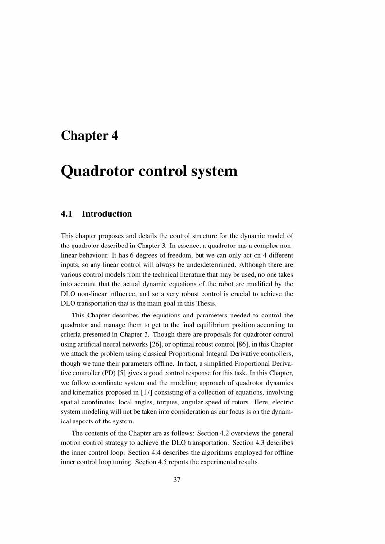
4 Quadrotor control system 374.1 Introduction . . . . . . . . . . . . . . . . . . . . . . . . . . . . . 374.2 General motion control for DLO transportation . . . . . . . . . . 384.3 Inner control loop . . . . . . . . . . . . . . . . . . . . . . . . . . 394.4 Offline inner control loop tuning . . . . . . . . . . . . . . . . . . 41
4.4.1 Ziegler-Nichols algorithm . . . . . . . . . . . . . . . . . 414.4.2 Particle Swarm Optimization (PSO) . . . . . . . . . . . . 41
4.5 Experiment 1 . . . . . . . . . . . . . . . . . . . . . . . . . . . . 434.5.1 Results of Experiment 1a . . . . . . . . . . . . . . . . . . 454.5.2 Results of Experiment 1b . . . . . . . . . . . . . . . . . . 47
4.6 Conclusions . . . . . . . . . . . . . . . . . . . . . . . . . . . . . 50
5 Transportation control 535.1 Introduction . . . . . . . . . . . . . . . . . . . . . . . . . . . . . 535.2 Quadrotor team control model . . . . . . . . . . . . . . . . . . . 545.3 Outer-loop control . . . . . . . . . . . . . . . . . . . . . . . . . 545.4 Outer control loop adaptive tuning . . . . . . . . . . . . . . . . . 565.5 Heuristics for smooth behaviors . . . . . . . . . . . . . . . . . . 585.6 Experiment 2 . . . . . . . . . . . . . . . . . . . . . . . . . . . . 58
5.6.1 Results of Experiment 2a . . . . . . . . . . . . . . . . . . 605.6.2 Results of Experiment 2b . . . . . . . . . . . . . . . . . 645.6.3 Results of Experiment 2c . . . . . . . . . . . . . . . . . 64
5.7 Experiment 3 . . . . . . . . . . . . . . . . . . . . . . . . . . . . 645.7.1 Results of Experiment 3a . . . . . . . . . . . . . . . . . . 695.7.2 Results of Experiment 3b . . . . . . . . . . . . . . . . . . 69
5.8 Conclusions . . . . . . . . . . . . . . . . . . . . . . . . . . . . . 72
6 Conclusions and Future Work 796.1 Conclusions . . . . . . . . . . . . . . . . . . . . . . . . . . . . . 79
6.1.1 Aerial robots modeling for cooperative transportation ofDLOs . . . . . . . . . . . . . . . . . . . . . . . . . . . . 79
6.1.2 Offline control strategy . . . . . . . . . . . . . . . . . . . 796.1.3 Online adaptive control strategy . . . . . . . . . . . . . . 80
6.2 Future Work . . . . . . . . . . . . . . . . . . . . . . . . . . . . . 806.2.1 System modeling . . . . . . . . . . . . . . . . . . . . . . 806.2.2 Control strategy . . . . . . . . . . . . . . . . . . . . . . . 81

CONTENTS xvii
Bibliography 82

xviii CONTENTS
List of Figures
1.1 Stylized physical representation of three drones carrying a DLOwhich is approximated by two catenary curve sections. . . . . . . 2
1.2 Roll, pitch and yaw angles representation . . . . . . . . . . . . . 5
2.1 Model to transport a payload in three dimensions through the airdescribed in [63] . . . . . . . . . . . . . . . . . . . . . . . . . . 13
2.2 2013 model for DLO transportation through the air . . . . . . . . 132.3 Hose model used in [81] . . . . . . . . . . . . . . . . . . . . . . 142.4 Catenary curve modeling a DLO holding between robots A and B. 152.5 Plus (left) and cross (right) rotor configurations . . . . . . . . . . 182.6 Plus configuration: pitch, roll and yaw controls, where red arrows
indicate the relative rotor speed . . . . . . . . . . . . . . . . . . . 192.7 Inner and outer loop for attitude and position . . . . . . . . . . . 222.8 PID controller diagram . . . . . . . . . . . . . . . . . . . . . . . 23
3.1 Catenary parameters (I,J) correspond to the catenary nodes . . . . 273.2 Catenary and two robots system . . . . . . . . . . . . . . . . . . 283.3 Catenary and three robots system. Initial state . . . . . . . . . . . 283.4 Plot of the differences with the desired state in Eq. 3.4. . . . . . . 293.5 Two fold catenary sustained by a three robots system. Initial (blue)
and final (red) states. . . . . . . . . . . . . . . . . . . . . . . . . 313.6 Two fold catenary sustained by three robot in an asymmetric initial
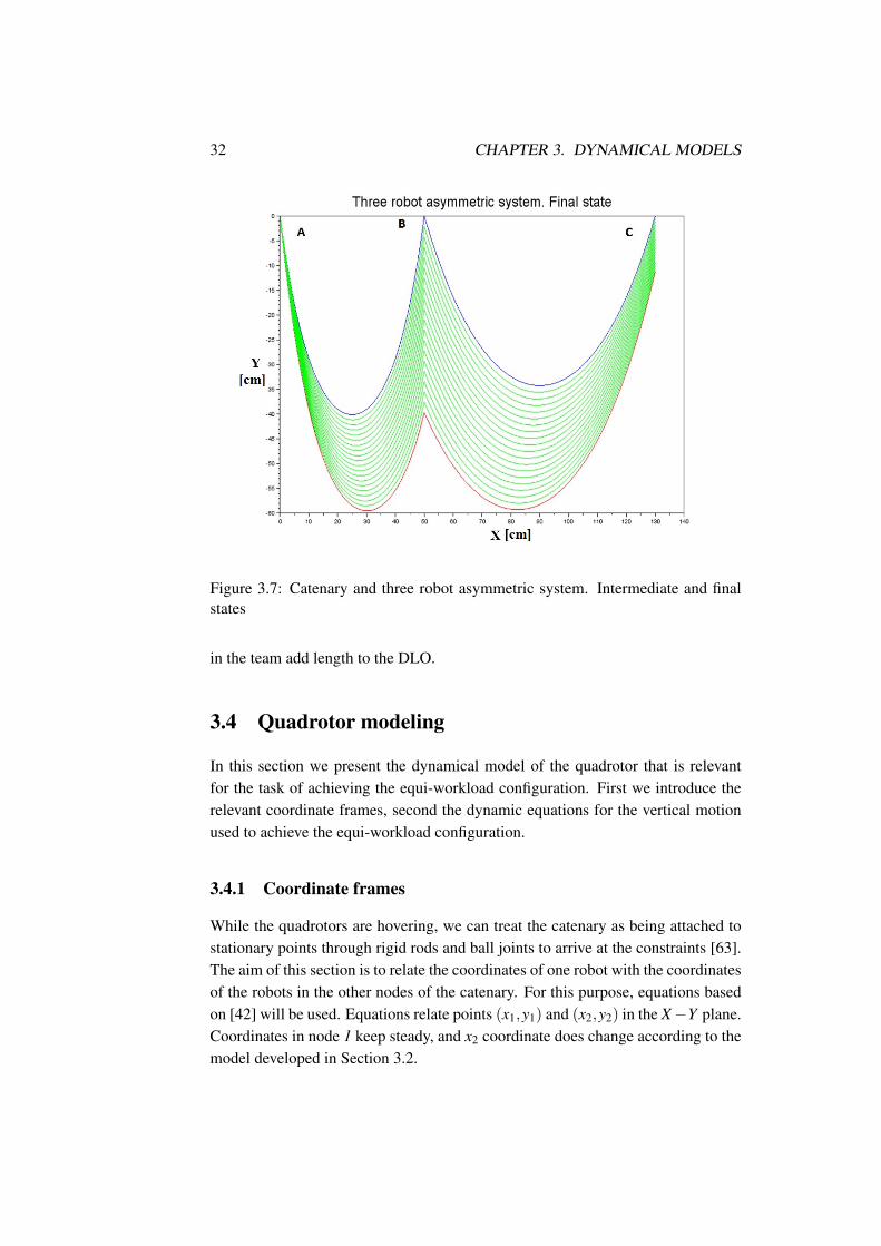
state. . . . . . . . . . . . . . . . . . . . . . . . . . . . . . . . . 313.7 Catenary and three robot asymmetric system. Intermediate and fi-
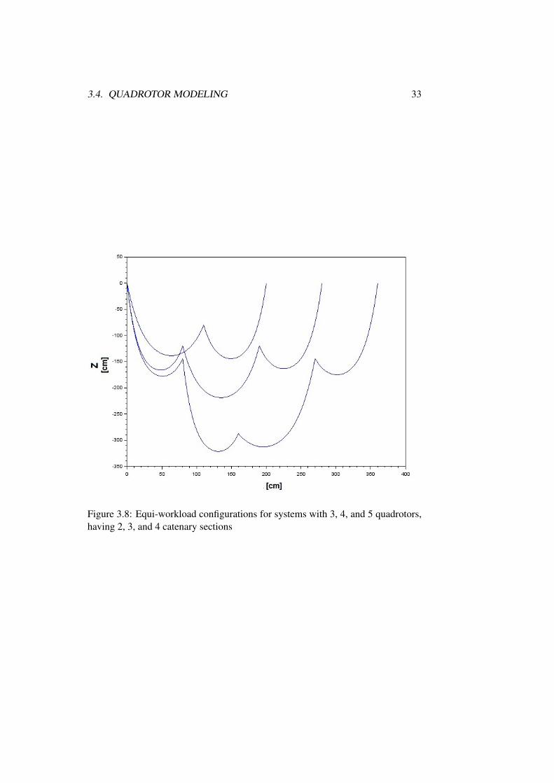
nal states . . . . . . . . . . . . . . . . . . . . . . . . . . . . . . . 323.8 Equi-workload configurations for systems with 3, 4, and 5 quadro-
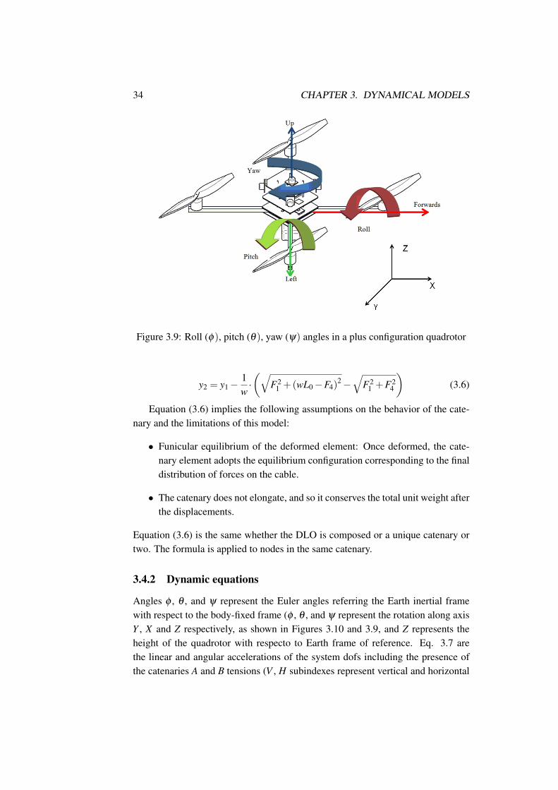
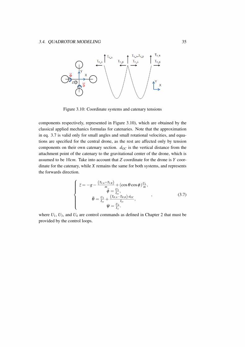
tors, having 2, 3, and 4 catenary sections . . . . . . . . . . . . . . 333.9 Roll (φ), pitch (θ), yaw (ψ) angles in a plus configuration quadrotor 343.10 Coordinate systems and catenary tensions . . . . . . . . . . . . . 35
4.1 Two loops controllers for quadrotor position and orientation . . . 38
xix
xx LIST OF FIGURES
4.2 Roll (φ), pitch (θ), yaw (ψ) angles in a plus configuration quadrotor 394.3 PID Z controller . . . . . . . . . . . . . . . . . . . . . . . . . . 404.4 PID φ controller . . . . . . . . . . . . . . . . . . . . . . . . . . . 404.5 PID θ controller . . . . . . . . . . . . . . . . . . . . . . . . . . . 404.6 PID ψ controller . . . . . . . . . . . . . . . . . . . . . . . . . . 414.7 Catenary and three robots system for Experiment 1a. Initial and
final state . . . . . . . . . . . . . . . . . . . . . . . . . . . . . . 444.8 Balanced catenary for Experiment 1b . . . . . . . . . . . . . . . . 454.9 Response of middle quadrotor in Figure 4.7, position in the Z co-
ordinate (elevation) under ZN tuning control to achieve the desiredstate of robot equiload. . . . . . . . . . . . . . . . . . . . . . . . 46
4.10 Response of quadrotor B of Figure 4.7, vertical speed under ZNtuning control to achieve the desired state of robot equiload. . . . 46
4.11 Response of quadrotor vertical B of Figure 4.7, vertical accelera-tion under ZN tuning control to achieve the desired state of robotequiload. . . . . . . . . . . . . . . . . . . . . . . . . . . . . . . . 47
4.12 Response of quadrotor vertical B of Figure 4.7, vertical displace-ment under PSO tuning control to achieve the desired state of robotequiload. Three different PD tuning combinations . . . . . . . . . 48
4.13 Response of quadrotor vertical B of Figure 4.7 Z displacement.Three different convergence heights . . . . . . . . . . . . . . . . 48
4.14 Response of quadrotor vertical B of Figure 4.7 vertical displace-ment under PSO for different dynamic parameters . . . . . . . . . 49
4.15 Response of quadrotor B of Figure 4.8, position in the Z coordinate(elevation) under the PID control to achieve the desired state ofrobot equiload after the extension of one of the catenaries due tochange in cruise speed of the C robot. . . . . . . . . . . . . . . . 50
4.16 Time plot of the load supported by quadrotor B of Figure 4.8 afterthe extension of one of the catenaries due to change in cruise speedof the C robot. . . . . . . . . . . . . . . . . . . . . . . . . . . . 51
5.1 Follow-the-leader behavior parameters: distance (λ ) between quadro-tors positions, and heading angular difference (ϕ) parameters. . . 55
5.2 Membership functions of the fuzzy adaption rules of the PD controlparameters . . . . . . . . . . . . . . . . . . . . . . . . . . . . . 56
5.3 Catenaries configuration for Experiment 2 . . . . . . . . . . . . . 605.4 Dependence of overshot in X (image a) and Y (image b) of robots
D1 and D2 on the required distance when training the controllersby minimizing CF1 in Experiment 2a . . . . . . . . . . . . . . . 61
LIST OF FIGURES xxi
5.5 Dependence of overshot in X (image a) and Y (image b) of robotsD1 and D2 on the required distance when training the controllersby minimizing CF2 in Experiment 2a . . . . . . . . . . . . . . . 62
5.6 Trajectory of the three quadrotors in (X ,Y ) space when the desiredmotion is (a) (4x,4y) = (60,30), (b) (4x,4y) = (140,60), forthe controllers achieved with both cost functions CF1 (up) and CF2(down). . . . . . . . . . . . . . . . . . . . . . . . . . . . . . . . 63
5.7 X (image a) and Y (image b) trajectory of three quadrotors in Ex-periment 2b . . . . . . . . . . . . . . . . . . . . . . . . . . . . . 65
5.8 Thrust of D1 and D2 in Experiment 2c under no disturbances . . . 66
5.9 Trajectory and thrust of drones under controllers trained minimiz-ing CF1 suffering wind disturbances in X direction in Experiment2c . . . . . . . . . . . . . . . . . . . . . . . . . . . . . . . . . . 67
5.10 Trajectory and thrust of drones under controllers trained minimiz-ing CF2 suffering wind disturbances in X direction in Experiment2c . . . . . . . . . . . . . . . . . . . . . . . . . . . . . . . . . . 67
5.11 Path of the leader quadrotor for the Experiment 3b . . . . . . . . . 67
5.12 Comparison offline PSO optimal estimation of PD controller pa-rameters vs online fuzzy modulated adaptive controller in Experi-ment 3a. a) Results without perturbations. b) Results under windconditions. . . . . . . . . . . . . . . . . . . . . . . . . . . . . . . 70
5.13 Trajectories of a system of four quadrotors in Experiment 3a with-out disturbances. Each color line corresponds to the motion of aquadrotor. (a), offline PSO optimal parameter setting of the con-troller. (b), online fuzzy modulated adaptive controller. . . . . . . 71
5.14 Trajectories of a system of four drones in Experiment 3b. (a), of-fline PSO optimal parameter setting. (b), online fuzzy modulatedadaptive controller. . . . . . . . . . . . . . . . . . . . . . . . . . 73
5.15 Error of offline PSO optimal parameter setting versus online fuzzymodulated adaptive controller following a curve path in Experi-ment 3b, increasing the number of quadrotors in the system. a)plot without wind shear infuence. b) wind frequency perturbationis set to its nominal value. . . . . . . . . . . . . . . . . . . . . . 74
5.16 Exploration of wind shear frequency impact on navigation error ofoffline PSO optimal parameter setting versus online fuzzy modu-lated adaptive controller following the curve path in Experiment 3bwith 4 drones . . . . . . . . . . . . . . . . . . . . . . . . . . . . 75
5.17 Time evolution of reference (blue) and real (red) values of the θ
and φ angles in a system of 3 quadrotors controlled by the fuzzyonline adaptive algorithm in the setting of Experiment 3b, for nowind conditions. Left and right column plots correspond to the θ
and φ angles of each robot, respectively. . . . . . . . . . . . . . . 765.18 Time evolution of reference (blue) and real (red) values of the dis-
tance between 3 quadrotors controlled by the fuzzy online adaptivealgorithm in the setting of Experiment 3b, for no wind conditions. 77
List of Tables
4.1 Ziegler-Nichols rules . . . . . . . . . . . . . . . . . . . . . . . . 424.2 Values of standard parrot quadrotor physical parameters. . . . . . 434.3 PSO parameters for Experiment 1 . . . . . . . . . . . . . . . . . 474.4 Values of AR Parrot [47] . . . . . . . . . . . . . . . . . . . . . . 49
5.1 PSO parameters for CF1 in Experiment 2 . . . . . . . . . . . . . 595.2 Values of standard parrot . . . . . . . . . . . . . . . . . . . . . . 685.3 Drones starting coordinates for Experiment 3 . . . . . . . . . . . 68

xxiv LIST OF TABLES
Chapter 1
Introduction
1.1 Introduction
The growing availability of cheap and robust quadrotors is making feasible inno-vative applications. A recently proposed challenging task for Unmanned AerialVehicles (UAV) is the transportation of deformable linear objects (DLO) [2], i.e.cables, by a team of quadrotors, which can be extremely useful in emergency situ-ations, such rescue operations in highly unstructured environments.
Controlling the motion of isolated quadrotors in obstacle free environmentshas been successfully achieved in the literature by optimized Proportional IntegralDerivative (PID) controllers [65]. However, solution of the control of a team ofquadrotors subject to non-linear interactions induced by a DLO hanging from themis far from being solved. In this regard, the works initiated in [31] and furtherdeveloped in this Thesis open a new venue of research, directly related to effortsof control of cooperative teams of aerial robots under the non-linear dynamicalinteractions introduced by the DLO linking.
Modeling DLO kinematics is a complex task requiring a compromise betweenmodel accuracy and computational cost [108]. Computing its reaction to externalforces involves careful modeling and optimization techniques. The DLO acts as apassive object that links otherwise isolated and independent quadrotors [28], intro-ducing dynamic interactions among the robots in the form of non-linear constraints.Previous works have dealt with dynamic modeling of the process of transporting aDLO by a team of mobile robots on a 2D surface [29].
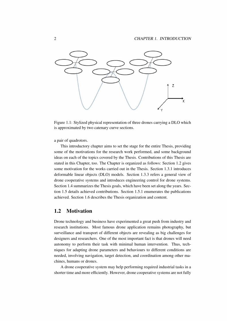
The physical configuration of an instance of the system with three quadrotors isrepresented in Figure 1.1, where three drones are sustaining a DLO hanging freelyin the space in stationary state. Non stationary regimes correspond to take-off andlanding of the robots, until they reach a height where the DLO does not touch anysurface. The DLO in Figure 1.1 appears divided in two sections each hanging from
1
2 CHAPTER 1. INTRODUCTION
Figure 1.1: Stylized physical representation of three drones carrying a DLO whichis approximated by two catenary curve sections.
a pair of quadrotors.This introductory chapter aims to set the stage for the entire Thesis, providing
some of the motivations for the research work performed, and some backgroundideas on each of the topics covered by the Thesis. Contributions of this Thesis arestated in this Chapter, too. The Chapter is organized as follows: Section 1.2 givessome motivation for the works carried out in the Thesis. Section 1.3.1 introducesdeformable linear objects (DLO) models. Section 1.3.3 refers a general view ofdrone cooperative systems and introduces engineering control for drone systems.Section 1.4 summarizes the Thesis goals, which have been set along the years. Sec-tion 1.5 details achieved contributions. Section 1.5.1 enumerates the publicationsachieved. Section 1.6 describes the Thesis organization and content.
1.2 Motivation
Drone technology and business have experimented a great push from industry andresearch institutions. Most famous drone application remains photography, butsurveillance and transport of different objects are revealing as big challenges fordesigners and researchers. One of the most important fact is that drones will needautonomy to perform their task with minimal human intervention. Thus, tech-niques for adapting drone parameters and behaviours to different conditions areneeded, involving navigation, target detection, and coordination among other ma-chines, humans or drones.
A drone cooperative system may help performing required industrial tasks in ashorter time and more efficiently. However, drone cooperative systems are not fully
1.3. ELEMENTARY DEFINITIONS 3
studied. As more drones are included in the team, or the task complexity increases,the correct drone coordination becomes a key issue. There, control happens to becritic, as it involves aspects as whether control is decentralized or centralized, orrearranges for any incidence, such a single drone failure in the swarm, or changingoutdoors perturbations. Thus, developing a robust control for these autonomouscooperative systems drones presents as a great technological and scientific chal-lenge for researchers and industry.
Packet delivery is turning out promising drone application for society. Thosepackets are habitually represented as regular small boxes, but after the launch ofthis idea some years ago, now unexplored alternatives start to rise up. How woulda swarm of drones be able to coordinate to transport a big packet? Or would a teamof aerial robots be capable of loading a deformable solid that could change theirdynamics continuously? In this Thesis, we combined the two previous mentionedpoints, and we developed a semi-autonomous cooperative drone system for thetransport of deformable linear objects.
DLO aerial transportation presents a wide range of potential applications. Someof them are listed next:
• Tethered quadrotors, which permit a continuous energy supply [104]
• ETH Institute for Dynamic Systems and Control published a video wherea team of quadrotors build autonomously a bridge made of ropes, which islater tested to support the crossing of a person. Their work was covered in[9] and [8], and the demo is located in their YouTube Channel 1.
• Second, SAP Group and Service-drone companies together carried out in2014 small tasks of a high-voltage line renewal with drones. Their video canbe found in Youtube2.
1.3 Elementary definitions
We include here some definitions that are recurrent along the Thesis report.
1.3.1 Deformable Linear Objects (DLO)
A DLO can be considered a single dimensional solid which acts as a passive ob-ject with strong dynamics linking the quadrotors, and influencing their dynamics.There are several examples of DLO models [107] such as wires, cables and ropes,which have different applications in industry [41], i.e. medical robots [67]. DLO
1https://www.youtube.com/watch?v=CCDIuZUfETc2https://www.youtube.com/watch?v=Cb6DBu8pHO0
4 CHAPTER 1. INTRODUCTION
geometrical and kinematics modeling is a complex task and requires a compro-mise between feasibility of the model and computational cost. Models of DLOhave been developed specifically to model rope manipulation to produce knots[58],[84]. Vibration damping of DLO has been dealt with fuzzy control and slidingmode control [27]. Reproducing the motion of the DLO in response to a force in-volves careful modeling and optimization techniques [60],[25]. Linked Multicom-ponent Robotic Systems (L-MCRS) [28] are a special case of DLO manipulatedby robots, whose dynamics have been studied in the case of ground mobile robots[29], achieving control by reinforcement learning [33][54].
1.3.2 Transport problem definition
The challenge of this Thesis work is to achieve robust navigation of a team ofquadrotors while carrying a DLO hanging from them. Robustness means that wewant the team to complete the task despite the perturbations introduced by the DLOnon-linear independent dynamics or external perturbations, such as wind shear ofvarious frequencies. Transportation means that the whole DLO is moved to an-other ground location from the initial one. We have identified two phases in thistask. First, setting the drones and DLO in an spatial configuration that imposesthe same workload to each quadrotor, an equi-workload configuration. Second, thetransportation per se that implies the motion of the whole system in the XY plane.
To do research on how to solve this problem we needed to attack two fronts.One is the accurate modeling of the DLO quadrotors system to be able to simulatethe system under diverse control and environmental conditions. The second is thedesign of robust control systems. If we assume quasy-stationary conditions theDLO can be modeled by sections of catenary curves, which allows very efficientimplementations of the system simulation. We try to achieve robust control byadaptive control approaches.
1.3.3 Quadrotor modeling and control
Although cooperative robot systems for collective intelligence purposes are widelystudied and big achievements are being obtained [83], cooperative drone systemsfor object transportation still remains an unexplored field. Few research groupshave created cooperative transportations [89] for quadrotors, but they still keep twobig differences with this Thesis: first, they do not attack the problem of deformablelinear objects fully, and secondly, they do not develop an efficient strategy for theirtransportation.
There are four input forces (one per rotor) and six output states (x,y, z, θ , φ ,ψ). Therefore, a quadrotor is an underactuated aircraft and modeling a vehicle suchthis is not an easy task because of its complex structure. The aim is to develop

1.4. THESIS GOALS 5
Figure 1.2: Roll, pitch and yaw angles representation
a model of the vehicle as realistic as possible. In the quadrotor, there are fourrotors with fixed angles which represent four input forces that are basically thethrust generated by each propeller, which create moments simulatenously. Thesemoments have been experimentally observed to be linearly dependent on the thrustforces at low speeds. The collective input is the sum of the thrusts of each motor.Pitch movement is obtained by increasing or reducing the speed of the rear motorwhile reducing or increasing the spped of the front motor. The roll movement isobtained similarly increasing or reducing the speeds on the right and left rotors.The yaw movement is obtained by varying the speed of the front and rear motorstogether while decreasing or increasing the speed of the lateral motors together.This should be done while keeping the total thrust constant. A representation ofthis model is shown in Figure 1.2.
The quadrotor dynamic modeling constrains the possibilities for engineeringcontrol strategies. In the bibliography, different alternatives are studied: PID con-trollers, LQR controllers, backstepping, robust, or optimal control algorithms, amongothers [118], [6]. In this Thesis, PID controllers were used. However, it is alsonecessary to obtain a good tuning methodology. The correct choice of these para-menters must guarantee convergence, stability, and adaptability in different stresssituations [57][100] [65].
1.4 Thesis goals
The main goal of this Thesis can be stated as follows:
1. Design of robust control systems for the transportation of a DLO by a team
6 CHAPTER 1. INTRODUCTION
of robots.
2. Experimental validation of the system under specific conditions.
From the operative point of view, we need to achieve specific goals:
1. Building an accurate dynamic simulation model of the DLO + quadrotorteam, in order to validate the control proposal in repeatable and controlledconditions. To achieve this goal we need to:
(a) Propose an accurate model of the DLO dynamics, that would also beefficient from the computational cost aspect.
(b) Build simulation models of the quadrotor.
2. Propose an overall team control strategy, i.e. how the drones coordinate toachieve the transportation task.
3. Define a spatial configuration of the quadrotors in which the energy con-sumption is the same for all, avoiding early energy depletion by some robots.
4. Propose robust drone control that carries out the desired task under the loadand perturbations induced by the DLO and external perturbations, such aswind.
(a) Offline tuning of the controllers
(b) Online adaptive tuning of the controllers
1.5 Thesis contributions
Pursuing the above goals, we have achieved several contributions. The main scien-tific results and contributions from this Thesis are the following:
1. We have proved that catenaries are suitable models for the dynamic repre-sentation of DLOs transportation by teams of quadrotors.
2. We have formalized a dynamic model that captures the dynamic behavior ofthe aerial robots together with the DLOs, which is adaptable to robots andDLOs with different physical and dynamic properties.
3. We have defined and computed the equi-workload spatial configuration, al-lowing equal energy consumption of all drones.
1.6. THESIS ORGANIZATION 7
4. We have proposed and published an innovative way of transporting DLOs,considering the quadrotors payload and difference of relative heights amongthem.
5. Defined of a leader-following strategy that ensures that distance limits amongdrones is kept along a straight or curved path.
6. We have obtained both offline and online control strategies that ensure therapid convergence of the system and its stability.
1.5.1 Publications achieved
• Estevez J., Lopez-Guede J. M., Graña M., (2014), “Quasi-stationary statetransportation of a DLO with quadrotors”. Robotics and Autonomous Sys-tems, Volume 63, Part 2, pp 187-194, ISSN 0921-8890.
• Lopez-Guede J. M., Estevez J., Graña J., Reinforcement Learning in SingleRobot DLO Transport Task: A Physical Proof of Concept, SOCO 2015 .
• Estevez J., Lopez-Guede J. M., Graña M., (2015), Robust Control Tuning byPSO of Aerial Robots DLO Transportation. IWINAC 2015.
• Estevez J., Lopez-Guede J. M., Graña M., (2015), “Robust Control Tuningby PSO of Aerial Robots DLO Transportation”. Bioinspired Computation inArtificial Systems 9108, pp 291-300. Springer.
• Estevez J., Lopez-Guede J. M., Graña M., (2016), “Particle Swarm Opti-mization quadrotor control for cooperative aerial transportation of deformablelinear objects”. Cybernetics and Systems. Vol. 47 (1-2), pp 4-16.
• Estevez J., Guisasola J., (2015) “El Taller del “Cuadricóptero” en la Sem-ana de la Ciencia. Divulgación de las aplicaciones científico-técnicas en lasociedad”. Revista Alambique (in press).
• Estevez J., Graña M., Lopez-Guede J.M., (2015), “Online fuzzy modulatedadaptive PD control for cooperative aerial transportation of deformable lin-ear objects”. Integrated Computer-Aided Engineering (submitted)
1.6 Thesis organization
The Thesis is organized as follows:
• Chapter 2 shows the State of the Art of the research lines. The aim of thischapter is to set the stage for different models and algorithms. Therefore, wecover in detail the literature for each aspect.
8 CHAPTER 1. INTRODUCTION
• Chapter 3 develops a dynamic model both for quadrotors and DLO. Here wepropose the catenary model for DLO, and give the dynamic equations of thequadrotors. This chapter is the basis for the development of a motion controlfor the cooperative system. Quadrotors’ dynamics are non-linear, and thusa precise and careful control is necessary. The control system is divided intwo parts.
• Chapter 4 explains the equi-workload configuration and its computation.Then we introduce the PD controller for inner loop control for altitude con-trol. We report computational experiments validating the approach.
• Chapter 5 discusses outer loop control for position control, proposing a novelfuzzy modulated adaptive tuning of the PD controllers. We report computa-tional experiments comparing offline and online approaches, to validate ourproposal.
• Chapter 6 ends with conclusions of the Thesis and some future work linesplanned to work on after current phase.
Chapter 2
State of the Art
In this Chapter we gather descriptions of the state of the art of the two researchlines mentioned in the introductory Chapter. The Chapter is structured as follows:Section 2.1 gives some basic definitions that will be used all along the Thesis.Section 2.2 presents a view of the state of the art on DLO modeling for differentapplications. Quadrotor modeling and control are divided in two sections: Section2.3 introduces the antecedents and problems of cooperative robotic systems. Sec-tion 2.4 gives the dynamical description of the quadrotor. Section 2.5 gives somebackground of quadrotors control and adaptive strategies.
2.1 Some basic definitions
Let us recall some definitions.
• Deformable Linear Object (DLO): As the definition states, these solidscan change their shape due to manipulation, representing a passive object.Due to the complexities of their representation, different simplifications areusually implemented for the simulation easiness.
• Cosserat rods: It is a physical model to represent DLO. The rod, which isassumed to undergo flexure about two principal axes, extension, shear andtorsion, are described by a general geometrically exact theory.
• Spline: it is a numeric function that is piecewise-defined by polynomialfunctions, and which possesses a high degree of smoothness at the placeswhere the polynomial pieces connect.
• Cooperative behavior: Given some task specified by a designer, a multiple-robot system displays cooperative behaviour if, due to some underlying mech-
9
10 CHAPTER 2. STATE OF THE ART
anism (i.e., the “mechanism of cooperation”), there is an increase in the totalutility of the system.
• Catenary curve: is the model of 2D rigid solid in quasy-stationary state,hanging freely from its two extremes.
2.2 Previous works on deformable linear objects models
Research on robotic manipulation has mainly focused on manipulating rigid ob-jects so far. However, many important application domains require manipulatingdeformable objects, especially deformable linear objects (DLO), such as ropes, ca-bles, and sutures. Such objects are very challenging to handle, as they can exhibita great diversity of behaviors. However, models that fully show dynamics, graphicrepresentation, material behaviour and deformation all together is an extreme dif-ficult task and it requires a very high computational cost. Thus, different modelshave emerged where one or two of DLO properties are finely represented whilesacrificing other ones, with a lower computational cost for online realistic simula-tions.
2.2.1 DLO modeling approaches
Two main representations are found in the bibliography: Cosserat rods and ge-ometric splines. In the robotics community, several recent works use Cosserattheory. A Cosserat medium was first described in 1909 by Cosserat brothers.This medium is described by a set of oriented micro-solids. [74] first introducedCosserat’s rod theory in computer graphics to model cantilever objects. This workfirst calculates the forces and torques iteratively along the rod discretization, andthen evaluates the geometrical configuration in backward iterations using differen-tial equations. [108] achieves a very accurate static solution of a cable simulationby considering it as a succession of oriented frames and by minimizing its potentialenergy; this approach is mechanically accurate, but demands a very high compu-tation cost. He uses Lagrangean formulation for his calculus, which gets a fastcomputation method and visually realistic for low resolution rods. [41] formulatesthe dynamic model of an inextensible DLO using finite element model (FEM) andLagrange motion equations including some dynamic effects, such as mass. Themain drawback of these methods is that it is difficult to combine such models withconstraints. Moreover, these methods need at least a reference point for calculation,which might not always be available in practical cases.
Spline-based techniques are still quite isolated within the physical animationliterature. [101] initiated deformable models in Computer Graphics, including
2.2. PREVIOUS WORKS ON DEFORMABLE LINEAR OBJECTS MODELS11
physics-based curves using a Lagrangian form of Newton’s equation. [45] simplystated, created an algorithm that divides a curve in segments of constant curvatureand solves the constrained energy minimization problem for a DLO manipulationpath planning. Later, [67] extended this idea to 3D, and made the algorithm morescalable to a higher number of segments. To simulate a deformable object, we needto compute any physically plausible configuration; not only stable configurations.The emphasis is on efficiency in computing the response of an object to internaland external forces. [78] uses a spline of linear springs, while [51] and [18] usedeformable splines for suture simulation in computer graphics, considering somesubtle dynamic effects.
However, these approaches do not consider the dynamic non-linearities thatDLO create when linked between different active agents. In order to model theseeffects, [79] developed dynamic NURBS, which is a combination of geometricsplines and physical models. Recently, in many of this kind of applications Geo-metric Dynamic Exact Splines (GEDS) are used, [103]. GEDS simply explained,represent a sum of geometric splines and Cosserat rods. For instance, it is used in[29] and [54] for the modeling of the transportation of deformable linear objectswith wheeled robots. However, the goal of this Thesis pursues the transportationof DLO through air, thus normally not considering transition states (taking off) orcontact against walls.
2.2.2 Aerial payload transportation using DLO
One situation when DLO are involved in transportation is when the payload to betransported is connected to the robots by DLO, i.e. some kind of cable. Though thecable is deformable, when it is transmitting the force of the robot to the payloadthe DLO acts as a rigid solid. Nevertheless, we review here some approaches inthe literature for the sake of completitude.
Though there are examples in the literature of robotic teams doing towing ofpayloads on the ground, there are significant differences between interacting withan object on the ground and in the air. The problem of swinging hanging payloadmanipulated by a robotic device has been studied for more than 30 years now.Certainly, in 1983 Gregory Starr [91] presented his work, Swing-free transportof suspended objects with a robot manipulator, later extended by [92], Swing-FreeTransport of Suspended Objects With a Path-Controlled Robot Manipulator, wherein both cases he used classical elementary applied mechanics equations for thesystem modeling. Despite the simplicity of the equations, his work lead to severalpatents, such as [87, 44, 40, 39].
After this initial step, following works pushed on a further study on this task,searching for robotic trajectories for payload transportation [93], vibration reduc-
12 CHAPTER 2. STATE OF THE ART
tion while performing this task [71], and development of control strategies forpayload manipulators [32] [111] [73]. Most works focused their efforts on sin-gle cable aerial towing of a payload, which applications go from personal rescueswith helicopter to heavy loads manipulation with cranes whose control is quitecomplex. First research works about UAVs transporting payloads appeared in late90’s [72][13]. In [23], the authors consider the problem of cooperative towing witha team of ground robots, where under quasi-static assumptions there is a uniquesolution to the motion of the object given the robot forces.
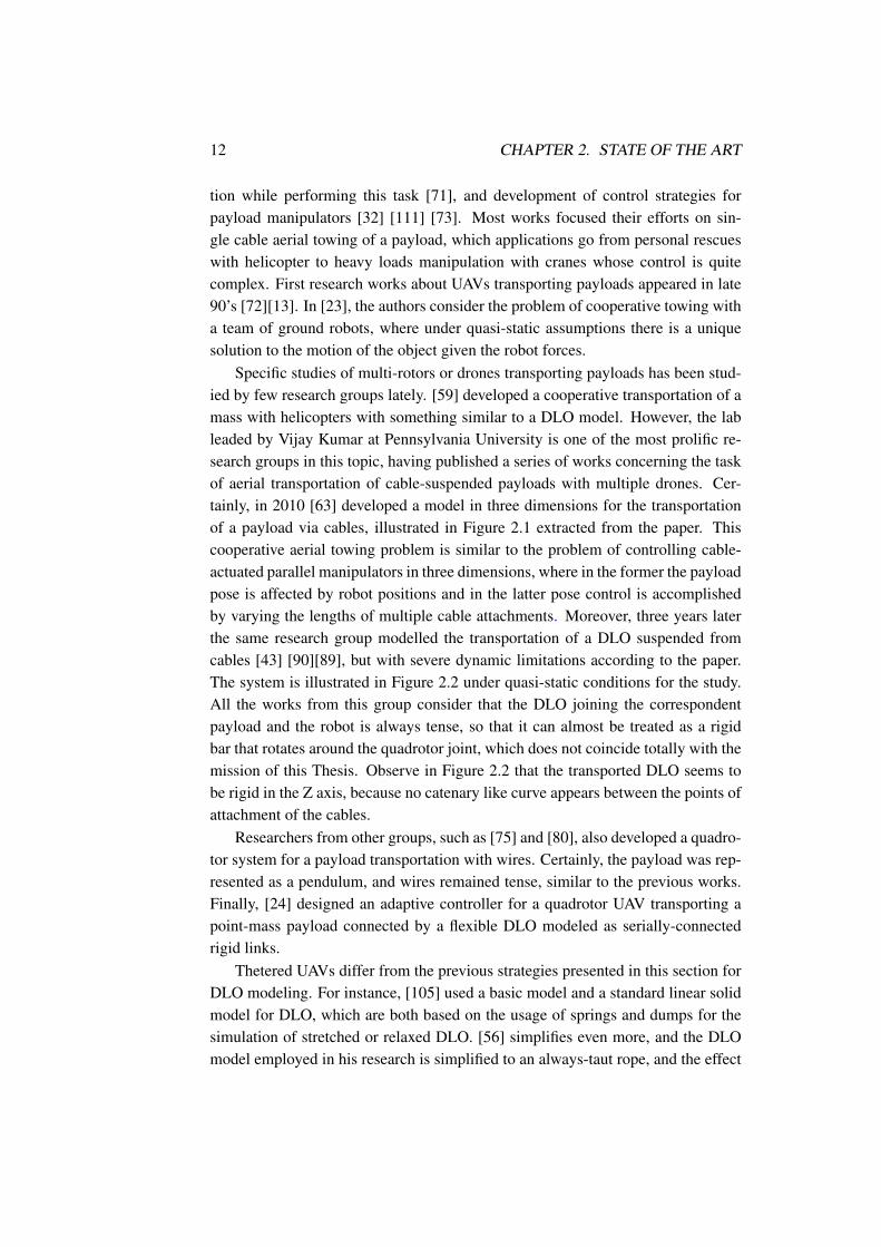
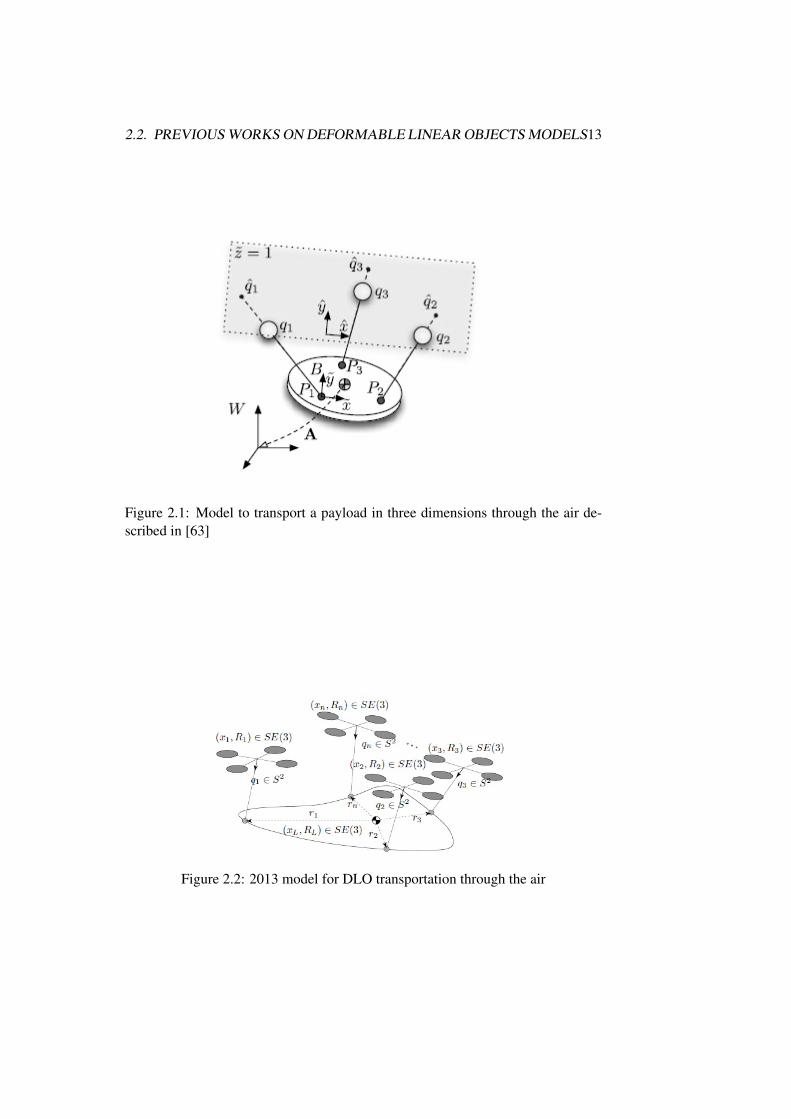
Specific studies of multi-rotors or drones transporting payloads has been stud-ied by few research groups lately. [59] developed a cooperative transportation of amass with helicopters with something similar to a DLO model. However, the lableaded by Vijay Kumar at Pennsylvania University is one of the most prolific re-search groups in this topic, having published a series of works concerning the taskof aerial transportation of cable-suspended payloads with multiple drones. Cer-tainly, in 2010 [63] developed a model in three dimensions for the transportationof a payload via cables, illustrated in Figure 2.1 extracted from the paper. Thiscooperative aerial towing problem is similar to the problem of controlling cable-actuated parallel manipulators in three dimensions, where in the former the payloadpose is affected by robot positions and in the latter pose control is accomplishedby varying the lengths of multiple cable attachments. Moreover, three years laterthe same research group modelled the transportation of a DLO suspended fromcables [43] [90][89], but with severe dynamic limitations according to the paper.The system is illustrated in Figure 2.2 under quasi-static conditions for the study.All the works from this group consider that the DLO joining the correspondentpayload and the robot is always tense, so that it can almost be treated as a rigidbar that rotates around the quadrotor joint, which does not coincide totally with themission of this Thesis. Observe in Figure 2.2 that the transported DLO seems tobe rigid in the Z axis, because no catenary like curve appears between the points ofattachment of the cables.
Researchers from other groups, such as [75] and [80], also developed a quadro-tor system for a payload transportation with wires. Certainly, the payload was rep-resented as a pendulum, and wires remained tense, similar to the previous works.Finally, [24] designed an adaptive controller for a quadrotor UAV transporting apoint-mass payload connected by a flexible DLO modeled as serially-connectedrigid links.
Thetered UAVs differ from the previous strategies presented in this section forDLO modeling. For instance, [105] used a basic model and a standard linear solidmodel for DLO, which are both based on the usage of springs and dumps for thesimulation of stretched or relaxed DLO. [56] simplifies even more, and the DLOmodel employed in his research is simplified to an always-taut rope, and the effect
2.2. PREVIOUS WORKS ON DEFORMABLE LINEAR OBJECTS MODELS13
Figure 2.1: Model to transport a payload in three dimensions through the air de-scribed in [63]
Figure 2.2: 2013 model for DLO transportation through the air
14 CHAPTER 2. STATE OF THE ART
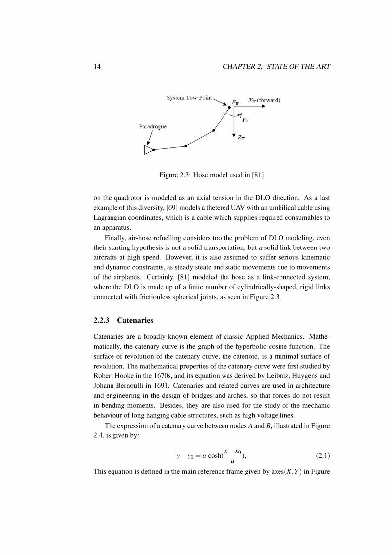
Figure 2.3: Hose model used in [81]
on the quadrotor is modeled as an axial tension in the DLO direction. As a lastexample of this diversity, [69] models a thetered UAV with an umbilical cable usingLagrangian coordinates, which is a cable which supplies required consumables toan apparatus.
Finally, air-hose refuelling considers too the problem of DLO modeling, eventheir starting hypothesis is not a solid transportation, but a solid link between twoaircrafts at high speed. However, it is also assumed to suffer serious kinematicand dynamic constraints, as steady steate and static movements due to movementsof the airplanes. Certainly, [81] modeled the hose as a link-connected system,where the DLO is made up of a finite number of cylindrically-shaped, rigid linksconnected with frictionless spherical joints, as seen in Figure 2.3.
2.2.3 Catenaries
Catenaries are a broadly known element of classic Applied Mechanics. Mathe-matically, the catenary curve is the graph of the hyperbolic cosine function. Thesurface of revolution of the catenary curve, the catenoid, is a minimal surface ofrevolution. The mathematical properties of the catenary curve were first studied byRobert Hooke in the 1670s, and its equation was derived by Leibniz, Huygens andJohann Bernoulli in 1691. Catenaries and related curves are used in architectureand engineering in the design of bridges and arches, so that forces do not resultin bending moments. Besides, they are also used for the study of the mechanicbehaviour of long hanging cable structures, such as high voltage lines.
The expression of a catenary curve between nodes A and B, illustrated in Figure2.4, is given by:
y− y0 = a·cosh(x− x0
a), (2.1)
This equation is defined in the main reference frame given by axes(X ,Y ) in Figure
2.2. PREVIOUS WORKS ON DEFORMABLE LINEAR OBJECTS MODELS15
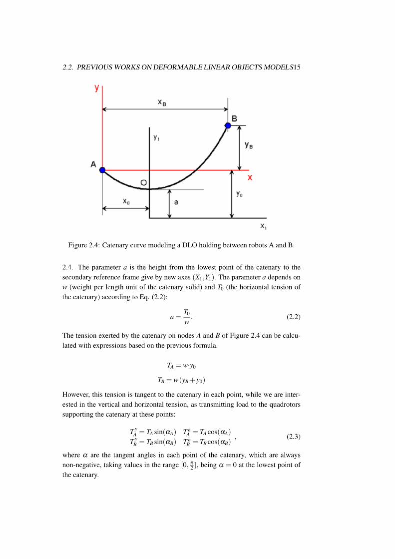
Figure 2.4: Catenary curve modeling a DLO holding between robots A and B.
2.4. The parameter a is the height from the lowest point of the catenary to thesecondary reference frame give by new axes (X1,Y1). The parameter a depends onw (weight per length unit of the catenary solid) and T0 (the horizontal tension ofthe catenary) according to Eq. (2.2):
a =T0
w. (2.2)
The tension exerted by the catenary on nodes A and B of Figure 2.4 can be calcu-lated with expressions based on the previous formula.
TA = w·y0
TB = w(yB + y0)
However, this tension is tangent to the catenary in each point, while we are inter-ested in the vertical and horizontal tension, as transmitting load to the quadrotorssupporting the catenary at these points:
T yA = TA sin(αA) T h
A = TA cos(αA)
T yB = TB sin(αB) T h
B = TB cos(αB), (2.3)
where α are the tangent angles in each point of the catenary, which are alwaysnon-negative, taking values in the range [0, π
2 ], being α = 0 at the lowest point ofthe catenary.
16 CHAPTER 2. STATE OF THE ART
The high aspect ratio of thin objects, such as paper and cloth, and linear objects,such as wire and thread, often causes instability in the computation of deformedshapes. Thus, various modeling techniques have been adapted for thin or linearobjects. For example, the deformed shape of a thread suspended by two pointshas been analyzed using calculus of variations and it has been found that the shapecan be described by a catenary [42]. In these approaches, the material propertiesare not considered; only the mass and quasi-static effects are considered. As thiselement is a rigid solid, deformations due to collisions cannot be modelled withsuch manner.
However, its usage as DLO modeling for robotics is only applied to cable-driven parallel robots, such as in [62] [48], who proposed an elastic catenary modelfor this kind of robots. On the other hand, [94], [4] and [37] perform a goodanalysis of effects of catenary joints and assumed hypothesis and considerations,both in 2D and 3D. Besides, the computer graphics cost, even in online simulations,is extremely low. [55] proposes a model for catenaries torsion and aerodynamiceffect inspired for hanging bridges. In summary, the application of catenaries toDLO transportation with quadrotors is an innovative contribution of this Thesis tothe State of the Art.
2.3 Drone cooperative systems
The study of multiple-robot systems naturally extends research done on single-robot systems, but it is also a discipline unto itself. Multiple-robot systems canaccomplish tasks that no single robot can accomplish, since ultimately a singlerobot, no matter how capable, is spatially limited:
• Tasks may be inherently too complex (or impossible) for a single robot to ac-complish, or performance benefits can be gained from using multiple robots.
• Building and using several simple robots can be easier, cheaper, more flex-ible and more fault-tolerant than having a single powerful robot for eachseparate task. Scalability is rewarded.
• The constructive, synthetic approach inherent in cooperative mobile roboticscan possibly yield insights into fundamental problems in the social sciences(organization theory, economics, cognitive psychology), and life sciences(theoretical biology, animal ethology).
• In case of payload transportation, sharing the load among a number of dronesturns the system into a more energy efficient one.
2.4. QUADROTOR DYNAMIC MODELING 17
In the literature, [21] and [76] provide a good study of the early antecedents andframework of this kind of systems. Coordination and interactions of multiple in-telligent agents have been actively studied in the field of distributed artificial in-telligence since the early 1970’s [12]. In the late 1980’s, the robotics researchcommunity became very active in cooperative robotics, beginning with projectssuch as CEBOT [34], SWARM [11], ACTRESS [7], and GOFER [20].
First research works about aerial cooperative robotic systems appeared in mid90’s [112], and this activity heavily increased in next decade, being of special in-terest for patrolling, fault-tolerant cooperation, swarm control, role assignment,multi-robot path planning, exploration and mapping, perimeter surveillance, andnowadays, collaborative learning.
In terms of practical value, one of the greatest benefits of the cooperative sys-tem is that it can provide users with superior information. However, developingsuch an autonomous cooperative system is quite challenging because of techni-cal and operation issues such as decision making, formation, path planning, to besolved. Control of the system might be centralized or decentralized.
• Centralized: means that all the information about the aerial robots is sentto a single server where the controls are calcultated for each aerial robot andsent back
• Decentralized: means that no central server exists, so that each aerial robotcomputes its own control based only on information from other aerial robotswithin a particular spatial range of itself. The situation is far from ideal underthe computational perspective because the number of aerial robots that canbe within range at a given time is bounded and therefore so is the time thealgorithm will take to run, regardless of the total number of aerial robotsinvolved.
2.4 Quadrotor dynamic modeling
A quadrotor is an agile flying vehicle, able to attain the full range of motions. Itis propelled by four rotors symmetrically disposed across its center. They havesmaller dimension and simple fabrication than conventional helicopters. Gener-ally, it should be classified as a rotary-wing aircraft according to its capability ofhover, perform horizontal flight, and vertical take-off and landing (VTOL). In thedecade of 1920, prototypes of manned quadrotors were introduced for the first time;however, the development of this new type of air vehicle was interrupted for sev-eral decades due to various reasons such as mechanical complexity, large size andweight, and difficulties in achieving robust stable control, especially. Only in re-cent years a great deal of interests and efforts have been attracted on it; a quadrotor
18 CHAPTER 2. STATE OF THE ART
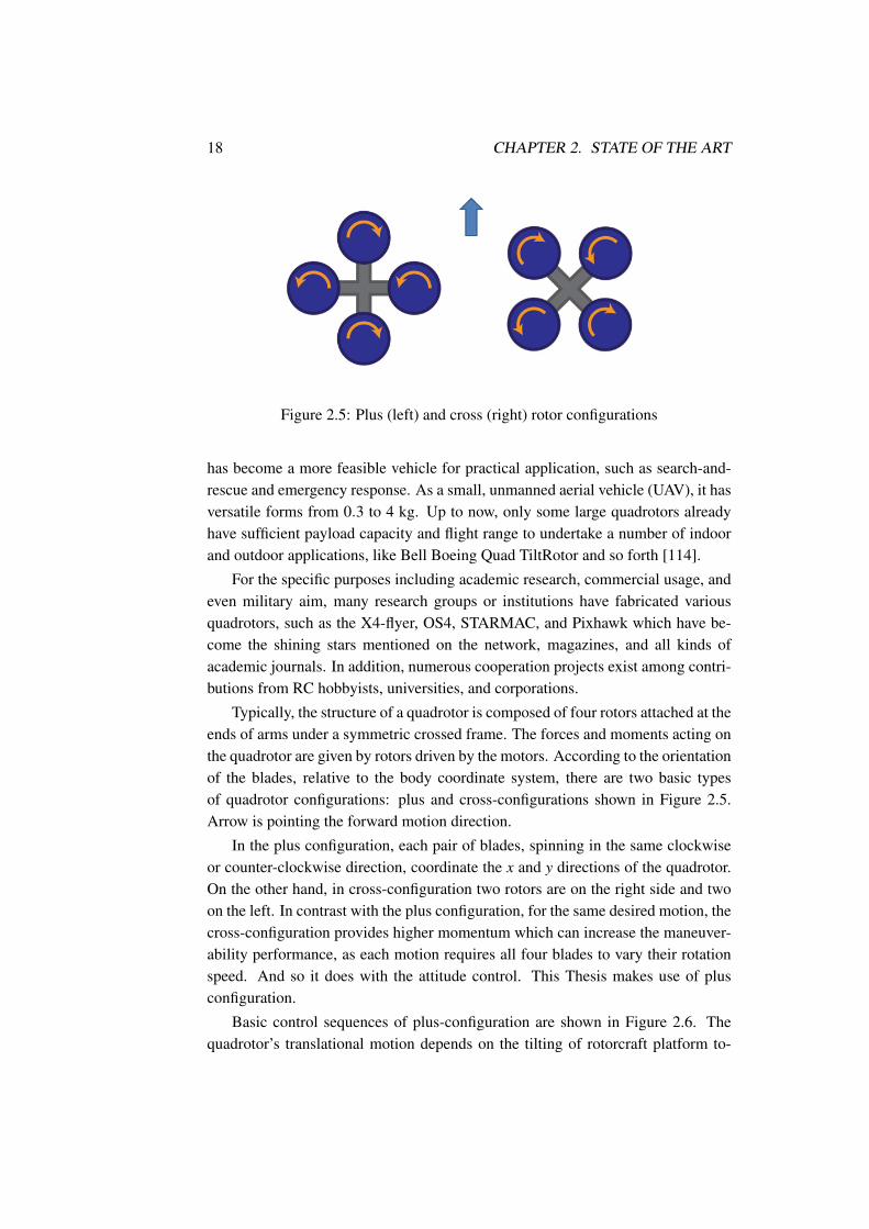
Figure 2.5: Plus (left) and cross (right) rotor configurations
has become a more feasible vehicle for practical application, such as search-and-rescue and emergency response. As a small, unmanned aerial vehicle (UAV), it hasversatile forms from 0.3 to 4 kg. Up to now, only some large quadrotors alreadyhave sufficient payload capacity and flight range to undertake a number of indoorand outdoor applications, like Bell Boeing Quad TiltRotor and so forth [114].
For the specific purposes including academic research, commercial usage, andeven military aim, many research groups or institutions have fabricated variousquadrotors, such as the X4-flyer, OS4, STARMAC, and Pixhawk which have be-come the shining stars mentioned on the network, magazines, and all kinds ofacademic journals. In addition, numerous cooperation projects exist among contri-butions from RC hobbyists, universities, and corporations.
Typically, the structure of a quadrotor is composed of four rotors attached at theends of arms under a symmetric crossed frame. The forces and moments acting onthe quadrotor are given by rotors driven by the motors. According to the orientationof the blades, relative to the body coordinate system, there are two basic typesof quadrotor configurations: plus and cross-configurations shown in Figure 2.5.Arrow is pointing the forward motion direction.
In the plus configuration, each pair of blades, spinning in the same clockwiseor counter-clockwise direction, coordinate the x and y directions of the quadrotor.On the other hand, in cross-configuration two rotors are on the right side and twoon the left. In contrast with the plus configuration, for the same desired motion, thecross-configuration provides higher momentum which can increase the maneuver-ability performance, as each motion requires all four blades to vary their rotationspeed. And so it does with the attitude control. This Thesis makes use of plusconfiguration.
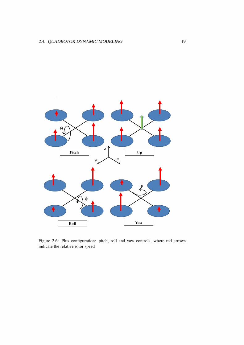
Basic control sequences of plus-configuration are shown in Figure 2.6. Thequadrotor’s translational motion depends on the tilting of rotorcraft platform to-
2.4. QUADROTOR DYNAMIC MODELING 19
Figure 2.6: Plus configuration: pitch, roll and yaw controls, where red arrowsindicate the relative rotor speed
20 CHAPTER 2. STATE OF THE ART
wards the desired orientation. The quadrotor has six degrees of freedom (DOF) tobe controlled by four inputs; therefore it is an underactuated system. In principle,a quadrotor is dynamically unstable and therefore careful control is necessary tomake it stable. Two main dynamic simulation approaches are widely accepted inthe literature for quadrotors:
• 1) Euler–Lagrange approach
• 2) Newton-Euler approach
Both methods lead to obtain same results in simulations, although Euler-Lagrangeis considered to have the advantage that it takes the same form in any system of gen-eralized coordinates, and it is better suited to generalizations and control adding.Typically two reference-frames are necessary to define the quadrotor’s dynamics:a body-fixed frame and Earth-fixed frame. However, exact and rigorous formulasderived from these approaches are fairly complex for control purposes, and thussome simplifications are implemented in most research works. These simplifiedformulas are the ones that appear in this section.
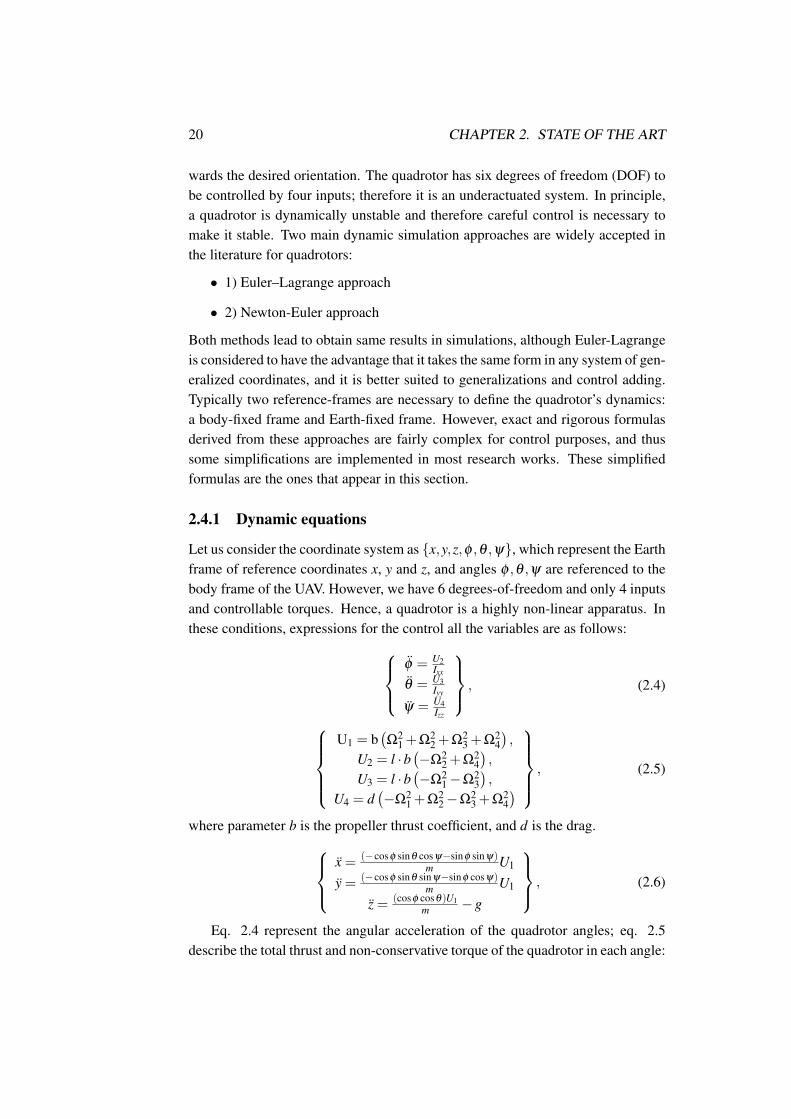
2.4.1 Dynamic equations
Let us consider the coordinate system as x,y,z,φ ,θ ,ψ, which represent the Earthframe of reference coordinates x, y and z, and angles φ ,θ ,ψ are referenced to thebody frame of the UAV. However, we have 6 degrees-of-freedom and only 4 inputsand controllable torques. Hence, a quadrotor is a highly non-linear apparatus. Inthese conditions, expressions for the control all the variables are as follows:
φ = U2Ixx
θ = U3Iyy
ψ = U4Izz
, (2.4)
U1 = b
(Ω2
1 +Ω22 +Ω2
3 +Ω24),
U2 = l ·b(−Ω2
2 +Ω24),
U3 = l ·b(−Ω2
1−Ω23),
U4 = d(−Ω2
1 +Ω22−Ω2
3 +Ω24) , (2.5)
where parameter b is the propeller thrust coefficient, and d is the drag.x = (−cosφ sinθ cosψ−sinφ sinψ)
m U1
y = (−cosφ sinθ sinψ−sinφ cosψ)m U1
z = (cosφ cosθ)U1m −g
, (2.6)
Eq. 2.4 represent the angular acceleration of the quadrotor angles; eq. 2.5describe the total thrust and non-conservative torque of the quadrotor in each angle:
2.5. CONTROL STRATEGIES 21
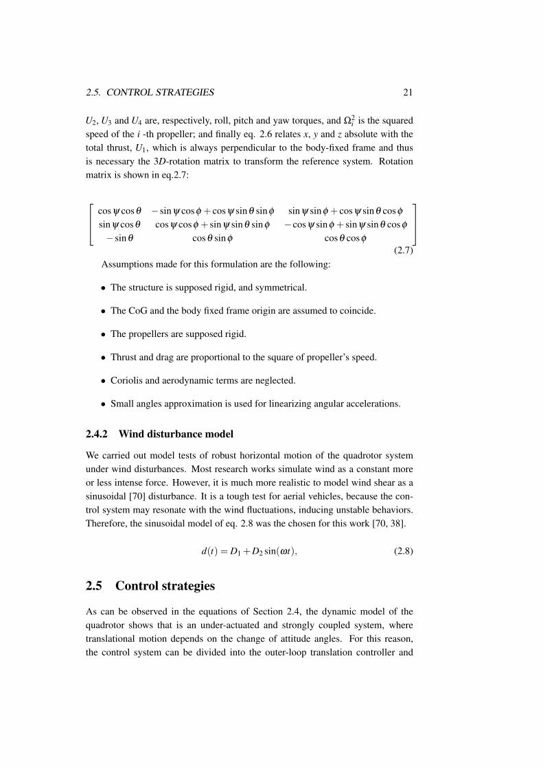
U2, U3 and U4 are, respectively, roll, pitch and yaw torques, and Ω2i is the squared
speed of the i -th propeller; and finally eq. 2.6 relates x, y and z absolute with thetotal thrust, U1, which is always perpendicular to the body-fixed frame and thusis necessary the 3D-rotation matrix to transform the reference system. Rotationmatrix is shown in eq.2.7:
cosψ cosθ −sinψ cosφ + cosψ sinθ sinφ sinψ sinφ + cosψ sinθ cosφ
sinψ cosθ cosψ cosφ + sinψ sinθ sinφ −cosψ sinφ + sinψ sinθ cosφ
−sinθ cosθ sinφ cosθ cosφ
(2.7)
Assumptions made for this formulation are the following:
• The structure is supposed rigid, and symmetrical.
• The CoG and the body fixed frame origin are assumed to coincide.
• The propellers are supposed rigid.
• Thrust and drag are proportional to the square of propeller’s speed.
• Coriolis and aerodynamic terms are neglected.
• Small angles approximation is used for linearizing angular accelerations.
2.4.2 Wind disturbance model
We carried out model tests of robust horizontal motion of the quadrotor systemunder wind disturbances. Most research works simulate wind as a constant moreor less intense force. However, it is much more realistic to model wind shear as asinusoidal [70] disturbance. It is a tough test for aerial vehicles, because the con-trol system may resonate with the wind fluctuations, inducing unstable behaviors.Therefore, the sinusoidal model of eq. 2.8 was the chosen for this work [70, 38].
d(t) = D1 +D2 sin(ωt), (2.8)
2.5 Control strategies
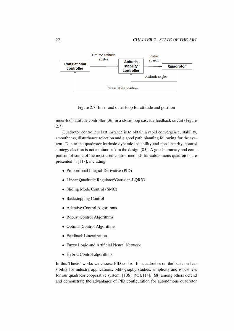
As can be observed in the equations of Section 2.4, the dynamic model of thequadrotor shows that is an under-actuated and strongly coupled system, wheretranslational motion depends on the change of attitude angles. For this reason,the control system can be divided into the outer-loop translation controller and
22 CHAPTER 2. STATE OF THE ART
Figure 2.7: Inner and outer loop for attitude and position
inner-loop attitude controller [36] in a close-loop cascade feedback circuit (Figure2.7).
Quadrotor controllers last instance is to obtain a rapid convergence, stability,smoothness, disturbance rejection and a good path planning following for the sys-tem. Due to the quadrotor intrinsic dynamic instability and non-linearity, controlstrategy election is not a minor task in the design [85]. A good summary and com-parison of some of the most used control methods for autonomous quadrotors arepresented in [118], including:
• Proportional Integral Derivative (PID)
• Linear Quadratic Regulator/Gaussian-LQR/G
• Sliding Mode Control (SMC)
• Backstepping Control
• Adaptive Control Algorithms
• Robust Control Algorithms
• Optimal Control Algorithms
• Feedback Linearization
• Fuzzy Logic and Artificial Neural Network
• Hybrid Control algorithms
In this Thesis’ works we choose PID control for quadrotors on the basis on fea-sibility for industry applications, bibliography studies, simplicity and robustnessfor our quadrotor cooperative system. [106], [95], [14], [68] among others defendand demonstrate the advantages of PID configuration for autonomous quadrotor
2.5. CONTROL STRATEGIES 23
Figure 2.8: PID controller diagram
systems against others. That way, the tuning of the control system reduces to thetuning of PID controllers discussed next.
2.5.1 PID tuning algorithms
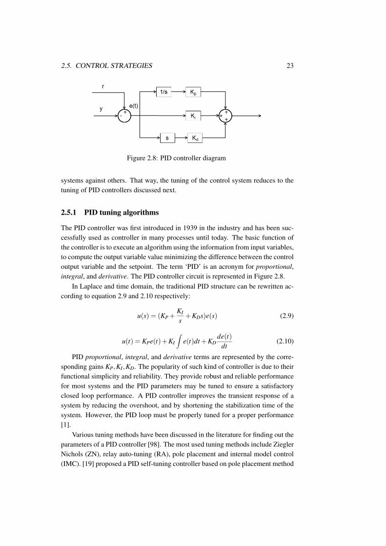
The PID controller was first introduced in 1939 in the industry and has been suc-cessfully used as controller in many processes until today. The basic function ofthe controller is to execute an algorithm using the information from input variables,to compute the output variable value minimizing the difference between the controloutput variable and the setpoint. The term ‘PID’ is an acronym for proportional,integral, and derivative. The PID controller circuit is represented in Figure 2.8.
In Laplace and time domain, the traditional PID structure can be rewritten ac-cording to equation 2.9 and 2.10 respectively:
u(s) = (KP +KI
s+KDs)e(s) (2.9)
u(t) = KPe(t)+KI
∫e(t)dt +KD
de(t)dt
(2.10)
PID proportional, integral, and derivative terms are represented by the corre-sponding gains KP,KI,KD. The popularity of such kind of controller is due to theirfunctional simplicity and reliability. They provide robust and reliable performancefor most systems and the PID parameters may be tuned to ensure a satisfactoryclosed loop performance. A PID controller improves the transient response of asystem by reducing the overshoot, and by shortening the stabilization time of thesystem. However, the PID loop must be properly tuned for a proper performance[1].
Various tuning methods have been discussed in the literature for finding out theparameters of a PID controller [98]. The most used tuning methods include ZieglerNichols (ZN), relay auto-tuning (RA), pole placement and internal model control(IMC). [19] proposed a PID self-tuning controller based on pole placement method
24 CHAPTER 2. STATE OF THE ART
for controlling an aluminum rolling mill. [117] proposed tuning of PID controllerwith time integral performance criteria, where ZN method was used to determiningthe controller parameters. [88] proposed a controller with a fuzzy model for air-conditioning system.
Different control schemes using PID controllers have been discussed in the lit-erature by various researchers. [77] proposed an internal model based robust inver-sion feed-forward and feedback control approach for LPV system while [114] pre-sented a discrete feed-forward and feedback optimal tracking control scheme for asteel jacket plat subjected to external wave force. [116] presented a comparativeanalysis between a single-loop control system and a cascade control system for athird-order process. [115] proposed model matching methods and approximate dy-namic inversion techniques for designing feed-forward controllers. A feed-forwardvelocity control scheme for a DC motor based on the inverse dynamic model hasbeen presented in the literature by [10]. A robust cascade control system has beenimplemented for controlling central air-conditioning system by [109]. [64] pro-posed a feed-forward control law based upon the concept of control equilibriumpoint.
Genetic Algorithm (GA) was proposed as an effective solution for the search inthe space of parameters for the optimal parameter setting. The fundamental compo-nents of GA are encoding, reproduction, crossover and mutation [99]. It has beenshown that GA could produce better results in PID tuning than the primitive tun-ing methods [49] having stochastic global searching characteristics that mimickingthe process of natural evolution. Later, a set of new intelligent approaches calledswarm intelligence tuning, such as Ant Colony Optimization, Particle Swarm Opti-mization (PSO) (first introduced by Kennedy and Eberhart in 1995 [46]), BacterialForaging optimization algorithm were introduced which could produce an effec-tive characteristics of positive feedback, search mechanism, distributed computa-tion and constructive greedy heuristic for simpler, efficient and faster tuning thanprimitive and other evolutionary tuning approaches for having improved character-istics like dynamic adjustment inertia weight factors, etc. Positive feedback searchproduces advantageous results, distributive computation can be used to avoid pre-matured convergence and greedy heuristic is helpful to find the solution of earlystages of search process.
Chapter 3
Dynamical models
3.1 Introduction
In this Chapter, we describe the dynamic models for the simulation of the aerialDLO transportation with quadrotors that will be used to tune and test the con-trollers for such task. As discussed in the state of the art of Chapter 2, there aredifferent approaches for modeling DLO, inspired in different disciplines such asmedicine, engineering, robotics, or computer graphics. However, most proposedmodels are subjected to certain modeling and behaviour restrictions due to the bigcomplexity and cost of processing. Our proposal is a novel way of modeling theDLO allowing to simulate the its transportation by aerial robots, i.e. quadrotors.Different quadrotor demos have shown that DLO transportation is feasible, how-ever in this Thesis we are concerned with developing robust control strategies.
The DLO model allows accurate modeling of the influence of DLO in quadro-tor dynamics in terms of thrust, weight or any other parameter that affects quadrotorbehaviour. Different quadrotor models exist, although they normally do not takeinto account the attachment of any payload. And as a final constraint, the modifiedquadrotor dynamics must admit any kind of engineering control which assures thatDLO transportation converges and happens smoothly.
The Chapter contents is as follows: Section 3.2 presents the modeling of theDLO as a collection of catenary curves, and its dynamical model, i.e. the resultingforces exerted on the quadrotors. Section 3.3 presents the derivation of the spatial(vertical) configuration of the quadrotor team where all the drones are supportingthe same load, and, thus, consuming the same quantity of energy. Section 3.4presents the dynamical model of the quadrotor, focused on the vertical dimensionto achieve the equi-workload spatial configuration.
25
26 CHAPTER 3. DYNAMICAL MODELS
3.2 Geometrical and dynamical DLO model
This section contains the description of the geometric and dynamical model of theDLO and the team of quadrotors carrying it. First, we justify and describe the DLOgeometrical model by a composition of catenary curves. Secondly, we give thecharacterization of the desired equi-workload configuration, and its computationfrom the geometrical/dynamical model.
Previous works on DLO transportation by a team of robots [29] were basedon a Generalized Dynamic Splines (GEDS) model of the DLO. GEDS are an ex-tension of the Cosserat rods models to capture the dynamics of a DLO. However,this approach has several drawbacks. The most critical is that the length of theDLO changes according to the settings of the spline model parameters. This isunacceptable for the case considered in present Thesis, because this effect wouldintroduce unreal random changes of altitude of the quadrotor UAVs. We will re-strict our study in the Thesis to the quasi-stationary state, when the drones are atcruise height and the DLO is freely hanging at full length. In this situation, theDLO can be modeled as a catenary curve [16], or a collection of catenary curvessharing their extreme points, and the deformations induced by its transportation canbe modeled by transformations between catenary curves. The catenary is the idealhyperbolic shape of a DLO whose unique load is its own weight, corresponding toa quasi-stationary state. It is the model of a perfect 2D rigid solid at equilibrium.Two drones (n = 2) can carry a catenary holding it at its end points (nodes). A longDLO divided in two sections, is transported by three drones (n = 3), and hence-forth, so that always n quadrotor UAVs carry a DLO composed of n− 1 sections.Each section will be modeled as an independent catenary curve without consider-ation of bending effects at the joining point. The study presented in this Chapterassumes two sections at most, but results are easily extrapolated to a greater num-ber of sections. Also, we deal with 2D catenary curves, but extension to 3D isimmediate [22]. Collision with ground surfaces render the catenary model inaccu-rate. They happen in the phases of take off and landing.
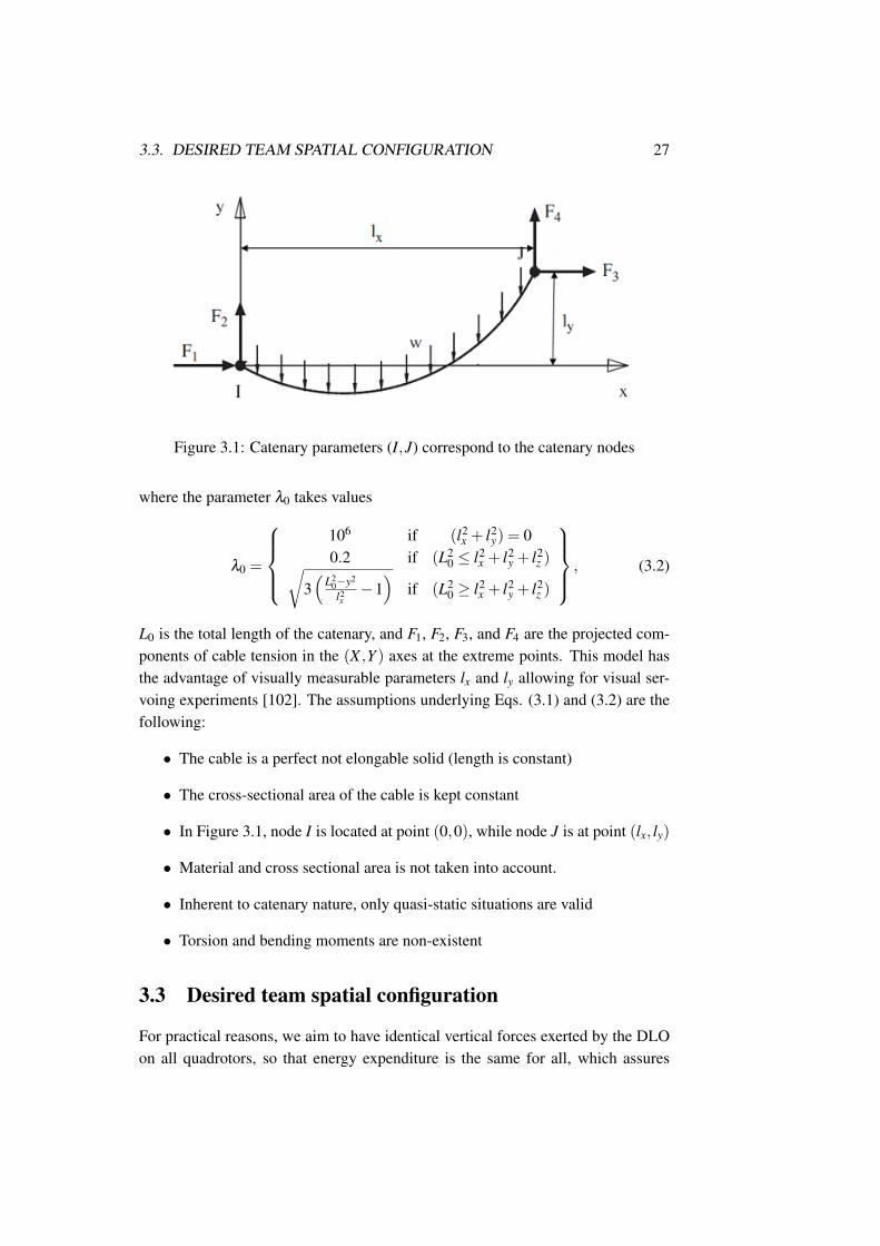
For real life experimentation requiring visual feedback, we need to reformulatethe conventional catenary model. This model, illustrated in Figure 3.1, is given bythe following equations:
F1 =− w·lx
2·λ0
F2 =w2 (−ly coth(λ0)+L0)
F3 =−F1
F4 = w·L0−F2
, (3.1)
3.3. DESIRED TEAM SPATIAL CONFIGURATION 27
Figure 3.1: Catenary parameters (I,J) correspond to the catenary nodes
where the parameter λ0 takes values
λ0 =
106 if (l2
x + l2y) = 0
0.2 if (L20 ≤ l2
x + l2y + l2
z )√3(
L20−y2
l2x−1)
if (L20 ≥ l2
x + l2y + l2
z )
, (3.2)
L0 is the total length of the catenary, and F1, F2, F3, and F4 are the projected com-ponents of cable tension in the (X ,Y ) axes at the extreme points. This model hasthe advantage of visually measurable parameters lx and ly allowing for visual ser-voing experiments [102]. The assumptions underlying Eqs. (3.1) and (3.2) are thefollowing:
• The cable is a perfect not elongable solid (length is constant)
• The cross-sectional area of the cable is kept constant
• In Figure 3.1, node I is located at point (0,0), while node J is at point (lx, ly)
• Material and cross sectional area is not taken into account.
• Inherent to catenary nature, only quasi-static situations are valid
• Torsion and bending moments are non-existent
3.3 Desired team spatial configuration
For practical reasons, we aim to have identical vertical forces exerted by the DLOon all quadrotors, so that energy expenditure is the same for all, which assures
28 CHAPTER 3. DYNAMICAL MODELS
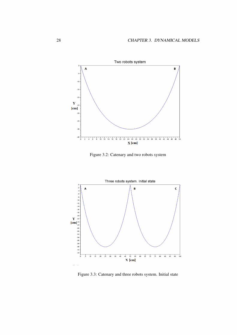
Figure 3.2: Catenary and two robots system
Figure 3.3: Catenary and three robots system. Initial state
3.3. DESIRED TEAM SPATIAL CONFIGURATION 29
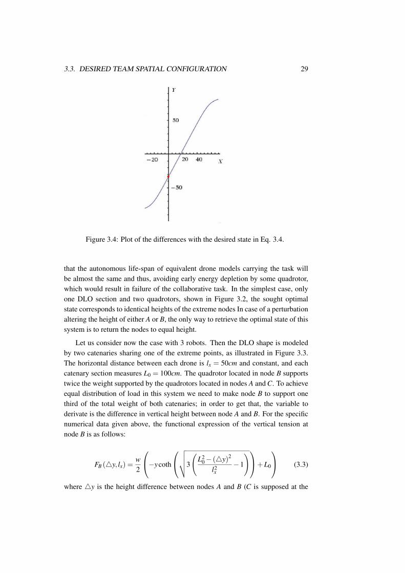
Figure 3.4: Plot of the differences with the desired state in Eq. 3.4.
that the autonomous life-span of equivalent drone models carrying the task willbe almost the same and thus, avoiding early energy depletion by some quadrotor,which would result in failure of the collaborative task. In the simplest case, onlyone DLO section and two quadrotors, shown in Figure 3.2, the sought optimalstate corresponds to identical heights of the extreme nodes In case of a perturbationaltering the height of either A or B, the only way to retrieve the optimal state of thissystem is to return the nodes to equal height.
Let us consider now the case with 3 robots. Then the DLO shape is modeledby two catenaries sharing one of the extreme points, as illustrated in Figure 3.3.The horizontal distance between each drone is lx = 50cm and constant, and eachcatenary section measures L0 = 100cm. The quadrotor located in node B supportstwice the weight supported by the quadrotors located in nodes A and C. To achieveequal distribution of load in this system we need to make node B to support onethird of the total weight of both catenaries; in order to get that, the variable toderivate is the difference in vertical height between node A and B. For the specificnumerical data given above, the functional expression of the vertical tension atnode B is as follows:
FB (4y, lx) =w2
−ycoth
√√√√3
(L2
0− (4y)2
l2x
−1
)+L0
(3.3)
where 4y is the height difference between nodes A and B (C is supposed at the
30 CHAPTER 3. DYNAMICAL MODELS
same height as A). Then the desired state is characterized by the following equality:
DF = FB (4y, lx)−(n−1)·w·L0
n= 0 (3.4)
Where n is the number of drones taking part in the cooperative transport system(n = 3 in current example) and DF represents the load difference among node Band any of the remaining nodes. Using the Newton-Raphson iterative method, min-imization of this function converges quickly using the expression of the gradient ofEq. (3.3) for the specific numerical values of the parameters given above:
∂
∂yFB (4y, lx) = F ′ =
w2
(-coth(A)−
√3·(4y)2 · 1
sinh2 (A)
l2x ·A
), (3.5)
where A is:
A =
√√√√3·
(L2
0− (4y)2
l2x
)−1
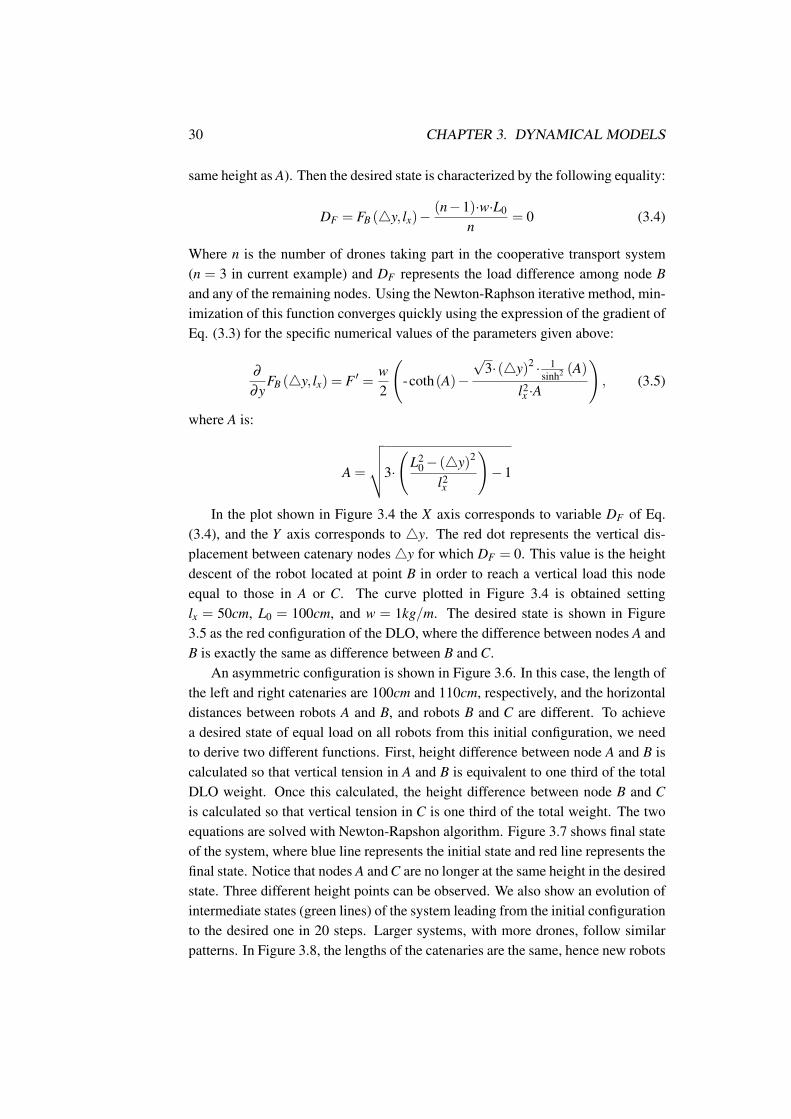
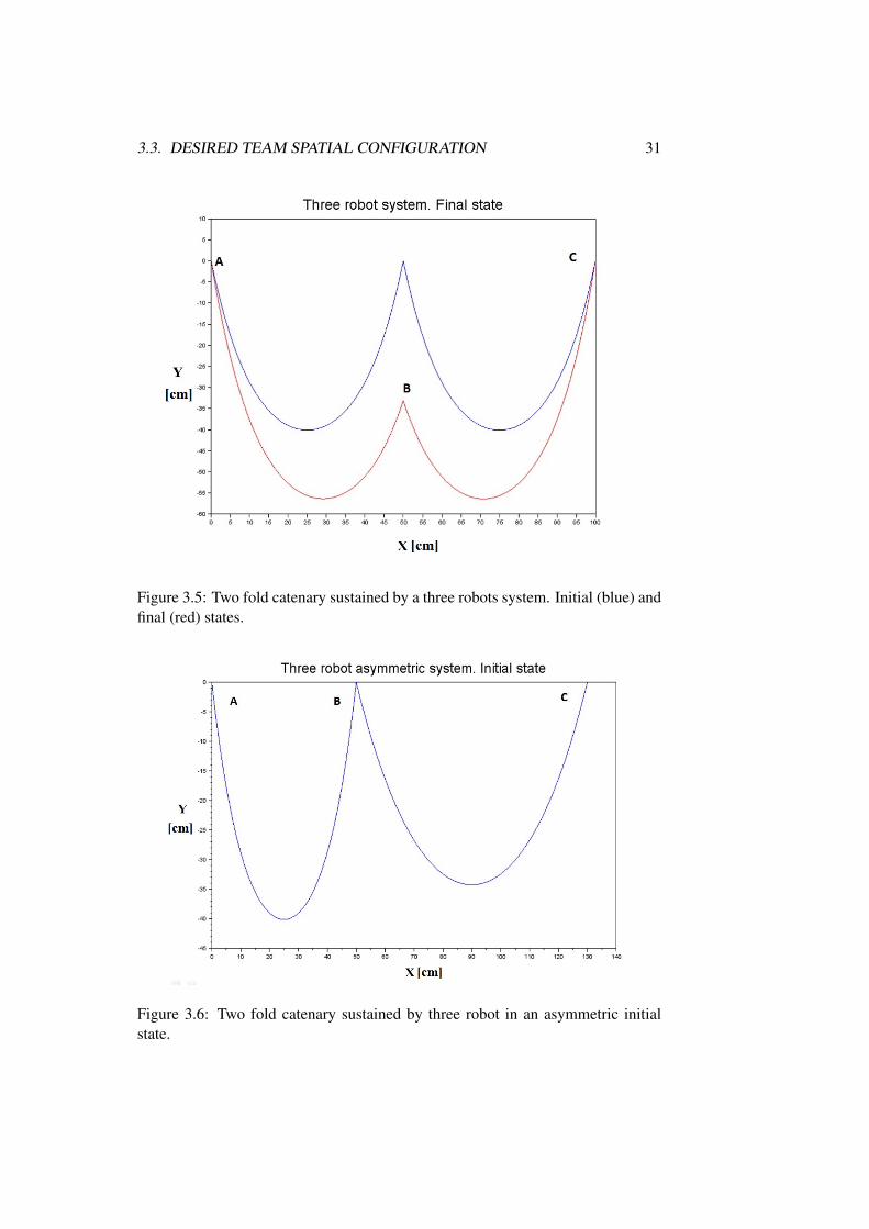
In the plot shown in Figure 3.4 the X axis corresponds to variable DF of Eq.(3.4), and the Y axis corresponds to 4y. The red dot represents the vertical dis-placement between catenary nodes4y for which DF = 0. This value is the heightdescent of the robot located at point B in order to reach a vertical load this nodeequal to those in A or C. The curve plotted in Figure 3.4 is obtained settinglx = 50cm, L0 = 100cm, and w = 1kg/m. The desired state is shown in Figure3.5 as the red configuration of the DLO, where the difference between nodes A andB is exactly the same as difference between B and C.
An asymmetric configuration is shown in Figure 3.6. In this case, the length ofthe left and right catenaries are 100cm and 110cm, respectively, and the horizontaldistances between robots A and B, and robots B and C are different. To achievea desired state of equal load on all robots from this initial configuration, we needto derive two different functions. First, height difference between node A and B iscalculated so that vertical tension in A and B is equivalent to one third of the totalDLO weight. Once this calculated, the height difference between node B and Cis calculated so that vertical tension in C is one third of the total weight. The twoequations are solved with Newton-Rapshon algorithm. Figure 3.7 shows final stateof the system, where blue line represents the initial state and red line represents thefinal state. Notice that nodes A and C are no longer at the same height in the desiredstate. Three different height points can be observed. We also show an evolution ofintermediate states (green lines) of the system leading from the initial configurationto the desired one in 20 steps. Larger systems, with more drones, follow similarpatterns. In Figure 3.8, the lengths of the catenaries are the same, hence new robots
3.3. DESIRED TEAM SPATIAL CONFIGURATION 31
Figure 3.5: Two fold catenary sustained by a three robots system. Initial (blue) andfinal (red) states.
Figure 3.6: Two fold catenary sustained by three robot in an asymmetric initialstate.
32 CHAPTER 3. DYNAMICAL MODELS
Figure 3.7: Catenary and three robot asymmetric system. Intermediate and finalstates
in the team add length to the DLO.
3.4 Quadrotor modeling
In this section we present the dynamical model of the quadrotor that is relevantfor the task of achieving the equi-workload configuration. First we introduce therelevant coordinate frames, second the dynamic equations for the vertical motionused to achieve the equi-workload configuration.
3.4.1 Coordinate frames
While the quadrotors are hovering, we can treat the catenary as being attached tostationary points through rigid rods and ball joints to arrive at the constraints [63].The aim of this section is to relate the coordinates of one robot with the coordinatesof the robots in the other nodes of the catenary. For this purpose, equations basedon [42] will be used. Equations relate points (x1,y1) and (x2,y2) in the X−Y plane.Coordinates in node 1 keep steady, and x2 coordinate does change according to themodel developed in Section 3.2.
3.4. QUADROTOR MODELING 33
Figure 3.8: Equi-workload configurations for systems with 3, 4, and 5 quadrotors,having 2, 3, and 4 catenary sections
34 CHAPTER 3. DYNAMICAL MODELS
Figure 3.9: Roll (φ), pitch (θ), yaw (ψ) angles in a plus configuration quadrotor
y2 = y1−1w·(√
F21 +(wL0−F4)
2−√
F21 +F2
4
)(3.6)
Equation (3.6) implies the following assumptions on the behavior of the cate-nary and the limitations of this model:
• Funicular equilibrium of the deformed element: Once deformed, the cate-nary element adopts the equilibrium configuration corresponding to the finaldistribution of forces on the cable.
• The catenary does not elongate, and so it conserves the total unit weight afterthe displacements.
Equation (3.6) is the same whether the DLO is composed or a unique catenary ortwo. The formula is applied to nodes in the same catenary.
3.4.2 Dynamic equations
Angles φ , θ , and ψ represent the Euler angles referring the Earth inertial framewith respect to the body-fixed frame (φ , θ , and ψ represent the rotation along axisY , X and Z respectively, as shown in Figures 3.10 and 3.9, and Z represents theheight of the quadrotor with respecto to Earth frame of reference. Eq. 3.7 arethe linear and angular accelerations of the system dofs including the presence ofthe catenaries A and B tensions (V , H subindexes represent vertical and horizontal
3.4. QUADROTOR MODELING 35
Figure 3.10: Coordinate systems and catenary tensions
components respectively, represented in Figure 3.10), which are obtained by theclassical applied mechanics formulas for catenaries. Note that the approximationin eq. 3.7 is valid only for small angles and small rotational velocities, and equa-tions are specified for the central drone, as the rest are affected only by tensioncomponents on their own catenary section. dGC is the vertical distance from theattachment point of the catenary to the gravitational center of the drone, which isassumed to be 10cm. Take into account that Z coordinate for the drone is Y coor-dinate for the catenary, while X remains the same for both systems, and representsthe forwards direction.
z =−g− (TV,A+TV,B)m +(cosθ cosφ)U1
m ,
φ = U2Ixx,
θ = U3Iyy
+(TH,A−TH,B)·dGC
Iyy,
ψ = U4Izz.
, (3.7)
where U1, U3, and U4 are control commands as defined in Chapter 2 that must beprovided by the control loops.

36 CHAPTER 3. DYNAMICAL MODELS
Chapter 4
Quadrotor control system
4.1 Introduction
This chapter proposes and details the control structure for the dynamic model ofthe quadrotor described in Chapter 3. In essence, a quadrotor has a complex non-linear behaviour. It has 6 degrees of freedom, but we can only act on 4 differentinputs, so any linear control will always be underdetermined. Although there arevarious control models from the technical literature that may be used, no one takesinto account that the actual dynamic equations of the robot are modified by theDLO non-linear influence, and so a very robust control is crucial to achieve theDLO transportation that is the main goal in this Thesis.
This Chapter describes the equations and parameters needed to control thequadrotor and manage them to get to the final equilibrium position according tocriteria presented in Chapter 3. Though there are proposals for quadrotor controlusing artificial neural networks [26], or optimal robust control [86], in this Chapterwe attack the problem using classical Proportional Integral Derivative controllers,though we tune their parameters offline. In fact, a simplified Proportional Deriva-tive controller (PD) [5] gives a good control response for this task. In this Chapter,we follow coordinate system and the modeling approach of quadrotor dynamicsand kinematics proposed in [17] consisting of a collection of equations, involvingspatial coordinates, local angles, torques, angular speed of rotors. Here, electricsystem modeling will not be taken into consideration as our focus is on the dynam-ical aspects of the system.
The contents of the Chapter are as follows: Section 4.2 overviews the generalmotion control strategy to achieve the DLO transportation. Section 4.3 describesthe inner control loop. Section 4.4 describes the algorithms employed for offlineinner control loop tuning. Section 4.5 reports the experimental results.
37
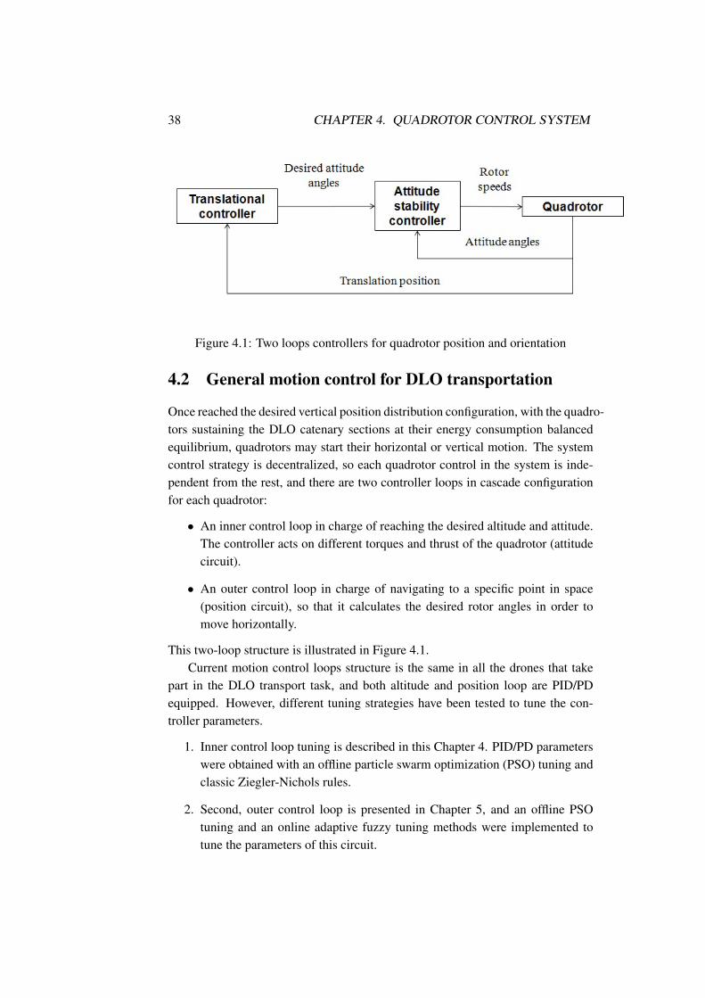
38 CHAPTER 4. QUADROTOR CONTROL SYSTEM
Figure 4.1: Two loops controllers for quadrotor position and orientation
4.2 General motion control for DLO transportation
Once reached the desired vertical position distribution configuration, with the quadro-tors sustaining the DLO catenary sections at their energy consumption balancedequilibrium, quadrotors may start their horizontal or vertical motion. The systemcontrol strategy is decentralized, so each quadrotor control in the system is inde-pendent from the rest, and there are two controller loops in cascade configurationfor each quadrotor:
• An inner control loop in charge of reaching the desired altitude and attitude.The controller acts on different torques and thrust of the quadrotor (attitudecircuit).
• An outer control loop in charge of navigating to a specific point in space(position circuit), so that it calculates the desired rotor angles in order tomove horizontally.
This two-loop structure is illustrated in Figure 4.1.Current motion control loops structure is the same in all the drones that take
part in the DLO transport task, and both altitude and position loop are PID/PDequipped. However, different tuning strategies have been tested to tune the con-troller parameters.
1. Inner control loop tuning is described in this Chapter 4. PID/PD parameterswere obtained with an offline particle swarm optimization (PSO) tuning andclassic Ziegler-Nichols rules.
2. Second, outer control loop is presented in Chapter 5, and an offline PSOtuning and an online adaptive fuzzy tuning methods were implemented totune the parameters of this circuit.

4.3. INNER CONTROL LOOP 39
Figure 4.2: Roll (φ), pitch (θ), yaw (ψ) angles in a plus configuration quadrotor
4.3 Inner control loop
We use four PD controllers for the roll, pitch, yaw and height, respectively, whichare the degrees of freedom (dof) of each quadrotor [17]. The block diagrams speci-fying the control of the degrees of freedom of each quadrotor are shown in Figures4.3, 4.4, 4.5, and 4.6. In the four control subsystems, the aim is that the real valueof the degree of freedom reaches the desired value, denoted by a d subindex. KP,KI , and KD are the three PID control parameters to be tuned. Finally, IXX , IYY , IZZ
[Nms2 or kgm2] are the body rotational moment of inertia around the X , Y and Zaxis.
The control system is scalable and can work with multiple drones. For greatersimplicity, the ψ degree of freedom is set to 0, so we will deal with PD controllers.The methodology to tune PD parameters of the quadrotor is described in Section4.4. In our experiments, all the quadrotors taking part in the system are equippedwith the same inner-loop PD parameters. In order to find them, two different exper-iments are carried out. In Experiment 1a, we carry out a comparison between thetwo offline tuning methods. In Experiment 1b, the robustness of chosen parametersin Experiment 1a is tested.
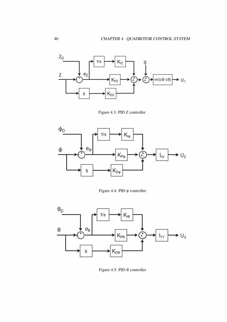
40 CHAPTER 4. QUADROTOR CONTROL SYSTEM
Figure 4.3: PID Z controller
Figure 4.4: PID φ controller
Figure 4.5: PID θ controller
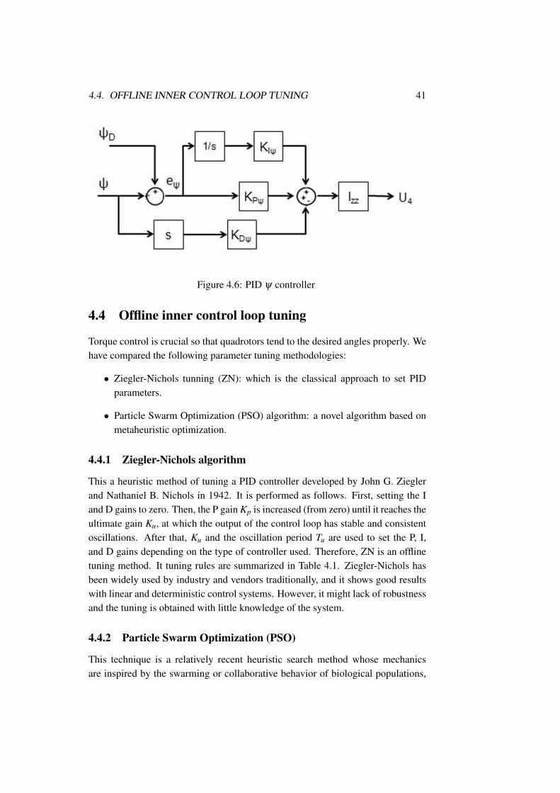
4.4. OFFLINE INNER CONTROL LOOP TUNING 41
Figure 4.6: PID ψ controller
4.4 Offline inner control loop tuning
Torque control is crucial so that quadrotors tend to the desired angles properly. Wehave compared the following parameter tuning methodologies:
• Ziegler-Nichols tunning (ZN): which is the classical approach to set PIDparameters.
• Particle Swarm Optimization (PSO) algorithm: a novel algorithm based onmetaheuristic optimization.
4.4.1 Ziegler-Nichols algorithm
This a heuristic method of tuning a PID controller developed by John G. Zieglerand Nathaniel B. Nichols in 1942. It is performed as follows. First, setting the Iand D gains to zero. Then, the P gain Kp is increased (from zero) until it reaches theultimate gain Ku, at which the output of the control loop has stable and consistentoscillations. After that, Ku and the oscillation period Tu are used to set the P, I,and D gains depending on the type of controller used. Therefore, ZN is an offlinetuning method. It tuning rules are summarized in Table 4.1. Ziegler-Nichols hasbeen widely used by industry and vendors traditionally, and it shows good resultswith linear and deterministic control systems. However, it might lack of robustnessand the tuning is obtained with little knowledge of the system.
4.4.2 Particle Swarm Optimization (PSO)
This technique is a relatively recent heuristic search method whose mechanicsare inspired by the swarming or collaborative behavior of biological populations,
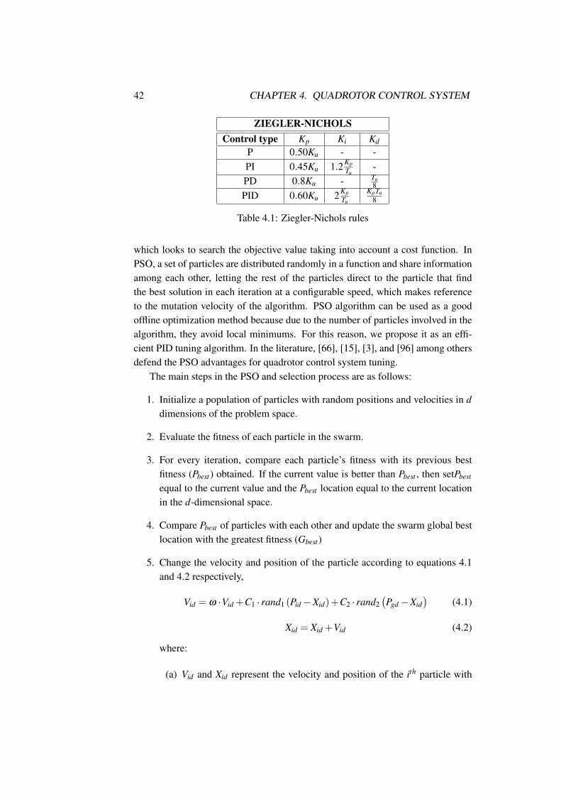
42 CHAPTER 4. QUADROTOR CONTROL SYSTEM
ZIEGLER-NICHOLSControl type Kp Ki Kd
P 0.50Ku - -PI 0.45Ku 1.2 Kp
Tu-
PD 0.8Ku - Tu8
PID 0.60Ku 2 KpTu
KpTu8
Table 4.1: Ziegler-Nichols rules
which looks to search the objective value taking into account a cost function. InPSO, a set of particles are distributed randomly in a function and share informationamong each other, letting the rest of the particles direct to the particle that findthe best solution in each iteration at a configurable speed, which makes referenceto the mutation velocity of the algorithm. PSO algorithm can be used as a goodoffline optimization method because due to the number of particles involved in thealgorithm, they avoid local minimums. For this reason, we propose it as an effi-cient PID tuning algorithm. In the literature, [66], [15], [3], and [96] among othersdefend the PSO advantages for quadrotor control system tuning.
The main steps in the PSO and selection process are as follows:
1. Initialize a population of particles with random positions and velocities in ddimensions of the problem space.
2. Evaluate the fitness of each particle in the swarm.
3. For every iteration, compare each particle’s fitness with its previous bestfitness (Pbest) obtained. If the current value is better than Pbest , then setPbest
equal to the current value and the Pbest location equal to the current locationin the d-dimensional space.
4. Compare Pbest of particles with each other and update the swarm global bestlocation with the greatest fitness (Gbest)
5. Change the velocity and position of the particle according to equations 4.1and 4.2 respectively,
Vid = ω ·Vid +C1 · rand1 (Pid−Xid)+C2 · rand2(Pgd−Xid
)(4.1)
Xid = Xid +Vid (4.2)
where:
(a) Vid and Xid represent the velocity and position of the ith particle with
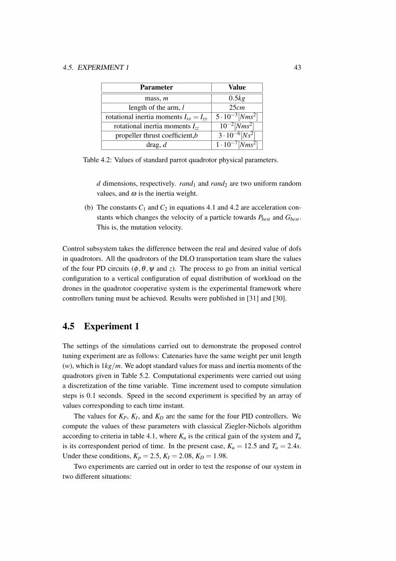
4.5. EXPERIMENT 1 43
Parameter Valuemass, m 0.5kg
length of the arm, l 25cmrotational inertia moments Ixx = Iyy 5 ·10−3[Nms2]
rotational inertia moments Izz 10−2[Nms2]
propeller thrust coefficient,b 3 ·10−6[Ns2]
drag, d 1 ·10−7[Nms2]
Table 4.2: Values of standard parrot quadrotor physical parameters.
d dimensions, respectively. rand1 and rand2 are two uniform randomvalues, and ω is the inertia weight.
(b) The constants C1 and C2 in equations 4.1 and 4.2 are acceleration con-stants which changes the velocity of a particle towards Pbest and Gbest .This is, the mutation velocity.
Control subsystem takes the difference between the real and desired value of dofsin quadrotors. All the quadrotors of the DLO transportation team share the valuesof the four PD circuits (φ ,θ ,ψ and z). The process to go from an initial verticalconfiguration to a vertical configuration of equal distribution of workload on thedrones in the quadrotor cooperative system is the experimental framework wherecontrollers tuning must be achieved. Results were published in [31] and [30].
4.5 Experiment 1
The settings of the simulations carried out to demonstrate the proposed controltuning experiment are as follows: Catenaries have the same weight per unit length(w), which is 1kg/m. We adopt standard values for mass and inertia moments of thequadrotors given in Table 5.2. Computational experiments were carried out usinga discretization of the time variable. Time increment used to compute simulationsteps is 0.1 seconds. Speed in the second experiment is specified by an array ofvalues corresponding to each time instant.
The values for KP, KI , and KD are the same for the four PID controllers. Wecompute the values of these parameters with classical Ziegler-Nichols algorithmaccording to criteria in table 4.1, where Ku is the critical gain of the system and Tu
is its correspondent period of time. In the present case, Ku = 12.5 and Tu = 2.4s.Under these conditions, Kp = 2.5, KI = 2.08, KD = 1.98.
Two experiments are carried out in order to test the response of our system intwo different situations:
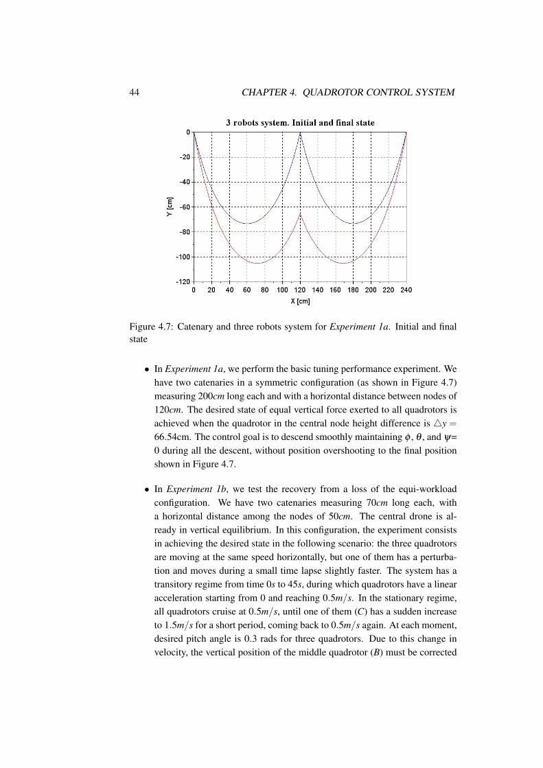
44 CHAPTER 4. QUADROTOR CONTROL SYSTEM
Figure 4.7: Catenary and three robots system for Experiment 1a. Initial and finalstate
• In Experiment 1a, we perform the basic tuning performance experiment. Wehave two catenaries in a symmetric configuration (as shown in Figure 4.7)measuring 200cm long each and with a horizontal distance between nodes of120cm. The desired state of equal vertical force exerted to all quadrotors isachieved when the quadrotor in the central node height difference is 4y =
66.54cm. The control goal is to descend smoothly maintaining φ , θ , and ψ=0 during all the descent, without position overshooting to the final positionshown in Figure 4.7.
• In Experiment 1b, we test the recovery from a loss of the equi-workloadconfiguration. We have two catenaries measuring 70cm long each, witha horizontal distance among the nodes of 50cm. The central drone is al-ready in vertical equilibrium. In this configuration, the experiment consistsin achieving the desired state in the following scenario: the three quadrotorsare moving at the same speed horizontally, but one of them has a perturba-tion and moves during a small time lapse slightly faster. The system has atransitory regime from time 0s to 45s, during which quadrotors have a linearacceleration starting from 0 and reaching 0.5m/s. In the stationary regime,all quadrotors cruise at 0.5m/s, until one of them (C) has a sudden increaseto 1.5m/s for a short period, coming back to 0.5m/s again. At each moment,desired pitch angle is 0.3 rads for three quadrotors. Due to this change invelocity, the vertical position of the middle quadrotor (B) must be corrected
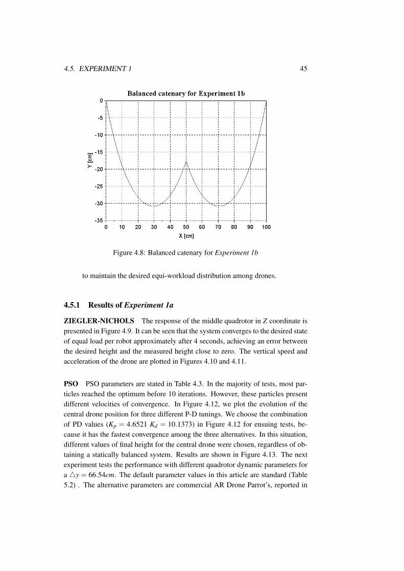
4.5. EXPERIMENT 1 45
Figure 4.8: Balanced catenary for Experiment 1b
to maintain the desired equi-workload distribution among drones.
4.5.1 Results of Experiment 1a
ZIEGLER-NICHOLS The response of the middle quadrotor in Z coordinate ispresented in Figure 4.9. It can be seen that the system converges to the desired stateof equal load per robot approximately after 4 seconds, achieving an error betweenthe desired height and the measured height close to zero. The vertical speed andacceleration of the drone are plotted in Figures 4.10 and 4.11.
PSO PSO parameters are stated in Table 4.3. In the majority of tests, most par-ticles reached the optimum before 10 iterations. However, these particles presentdifferent velocities of convergence. In Figure 4.12, we plot the evolution of thecentral drone position for three different P-D tunings. We choose the combinationof PD values (Kp = 4.6521 Kd = 10.1373) in Figure 4.12 for ensuing tests, be-cause it has the fastest convergence among the three alternatives. In this situation,different values of final height for the central drone were chosen, regardless of ob-taining a statically balanced system. Results are shown in Figure 4.13. The nextexperiment tests the performance with different quadrotor dynamic parameters fora 4y = 66.54cm. The default parameter values in this article are standard (Table5.2) . The alternative parameters are commercial AR Drone Parrot’s, reported in
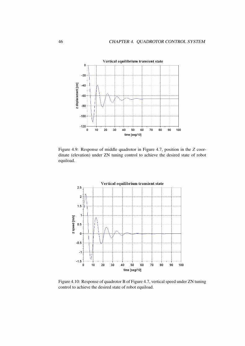
46 CHAPTER 4. QUADROTOR CONTROL SYSTEM
Figure 4.9: Response of middle quadrotor in Figure 4.7, position in the Z coor-dinate (elevation) under ZN tuning control to achieve the desired state of robotequiload.
Figure 4.10: Response of quadrotor B of Figure 4.7, vertical speed under ZN tuningcontrol to achieve the desired state of robot equiload.
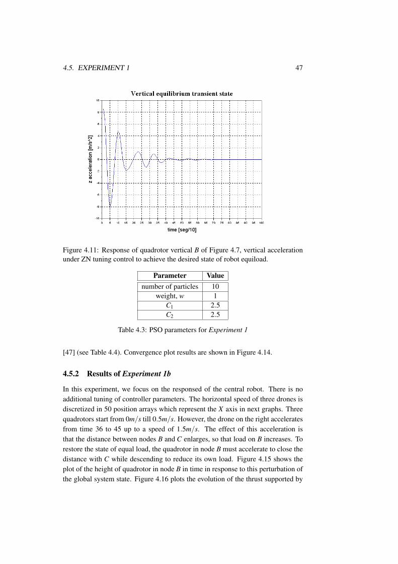
4.5. EXPERIMENT 1 47
Figure 4.11: Response of quadrotor vertical B of Figure 4.7, vertical accelerationunder ZN tuning control to achieve the desired state of robot equiload.
Parameter Valuenumber of particles 10
weight, w 1C1 2.5C2 2.5
Table 4.3: PSO parameters for Experiment 1
[47] (see Table 4.4). Convergence plot results are shown in Figure 4.14.
4.5.2 Results of Experiment 1b
In this experiment, we focus on the responsed of the central robot. There is noadditional tuning of controller parameters. The horizontal speed of three drones isdiscretized in 50 position arrays which represent the X axis in next graphs. Threequadrotors start from 0m/s till 0.5m/s. However, the drone on the right acceleratesfrom time 36 to 45 up to a speed of 1.5m/s. The effect of this acceleration isthat the distance between nodes B and C enlarges, so that load on B increases. Torestore the state of equal load, the quadrotor in node B must accelerate to close thedistance with C while descending to reduce its own load. Figure 4.15 shows theplot of the height of quadrotor in node B in time in response to this perturbation ofthe global system state. Figure 4.16 plots the evolution of the thrust supported by
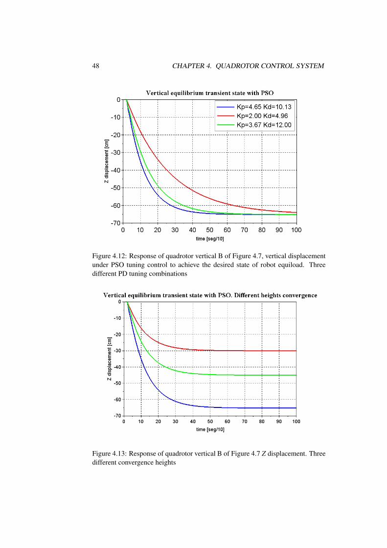
48 CHAPTER 4. QUADROTOR CONTROL SYSTEM
Figure 4.12: Response of quadrotor vertical B of Figure 4.7, vertical displacementunder PSO tuning control to achieve the desired state of robot equiload. Threedifferent PD tuning combinations
Figure 4.13: Response of quadrotor vertical B of Figure 4.7 Z displacement. Threedifferent convergence heights
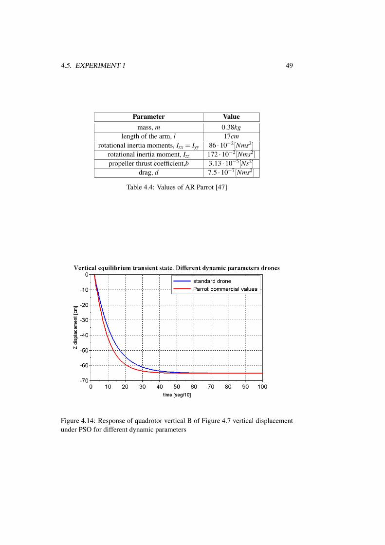
4.5. EXPERIMENT 1 49
Parameter Valuemass, m 0.38kg
length of the arm, l 17cmrotational inertia moments, Ixx = Iyy 86 ·10−2[Nms2]
rotational inertia moment, Izz 172 ·10−2[Nms2]
propeller thrust coefficient,b 3.13 ·10−5[Ns2]
drag, d 7.5 ·10−7[Nms2]
Table 4.4: Values of AR Parrot [47]
Figure 4.14: Response of quadrotor vertical B of Figure 4.7 vertical displacementunder PSO for different dynamic parameters
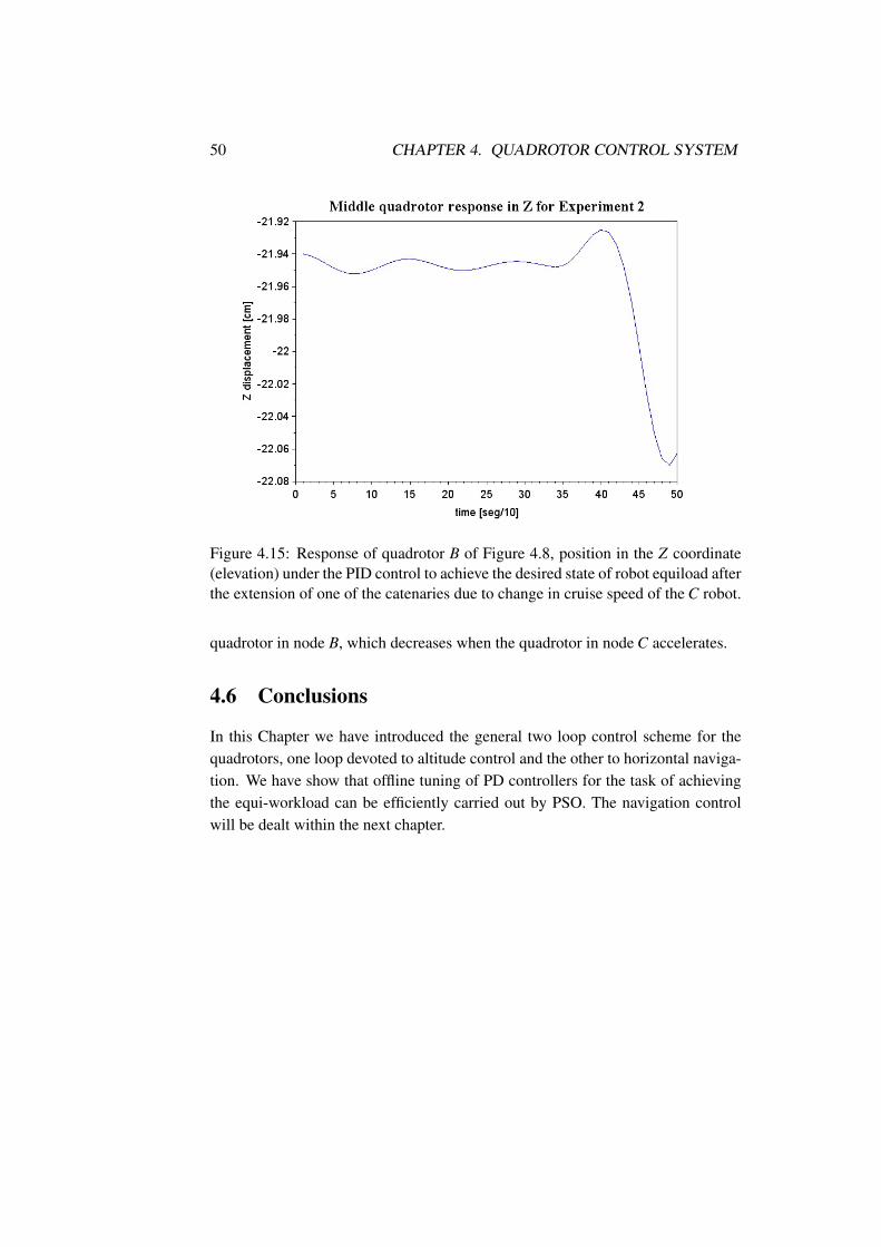
50 CHAPTER 4. QUADROTOR CONTROL SYSTEM
Figure 4.15: Response of quadrotor B of Figure 4.8, position in the Z coordinate(elevation) under the PID control to achieve the desired state of robot equiload afterthe extension of one of the catenaries due to change in cruise speed of the C robot.
quadrotor in node B, which decreases when the quadrotor in node C accelerates.
4.6 Conclusions
In this Chapter we have introduced the general two loop control scheme for thequadrotors, one loop devoted to altitude control and the other to horizontal naviga-tion. We have show that offline tuning of PD controllers for the task of achievingthe equi-workload can be efficiently carried out by PSO. The navigation controlwill be dealt within the next chapter.
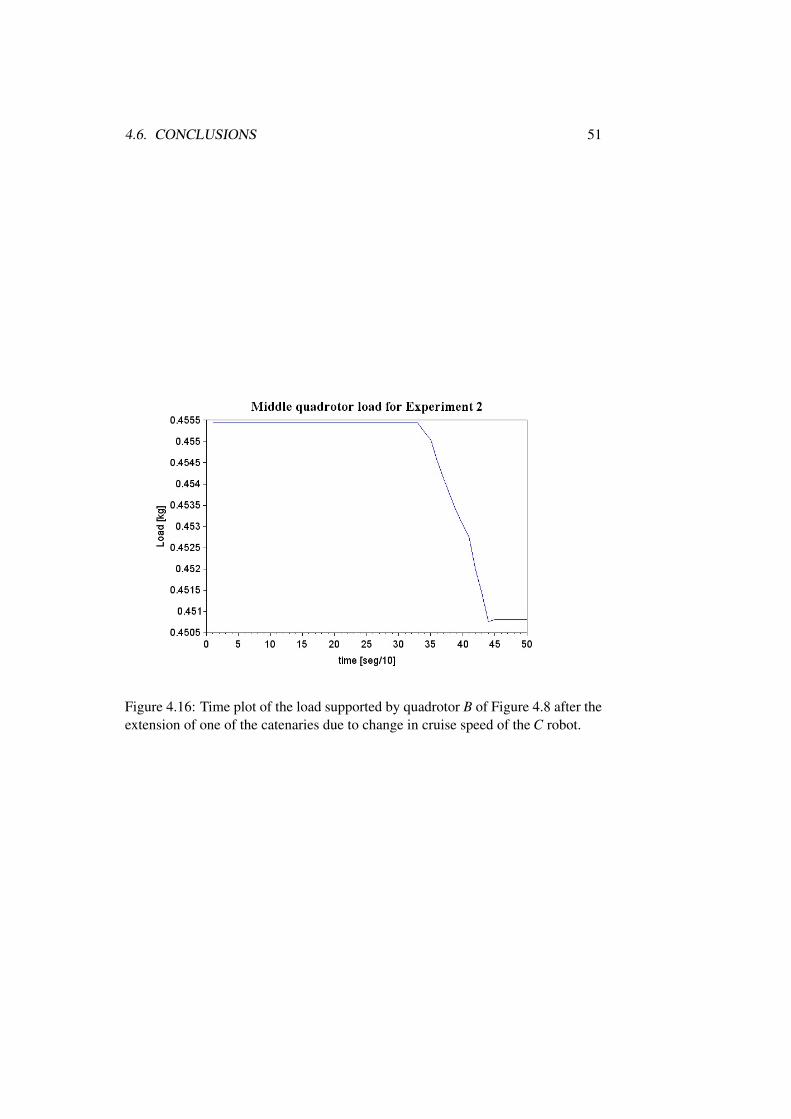
4.6. CONCLUSIONS 51
Figure 4.16: Time plot of the load supported by quadrotor B of Figure 4.8 after theextension of one of the catenaries due to change in cruise speed of the C robot.
52 CHAPTER 4. QUADROTOR CONTROL SYSTEM
Chapter 5
Transportation control
5.1 Introduction
This Chapter presents the second part of the quadrotor control structure for the taskof team DLO transportation, which is in charge of tuning the outer-loop control,i.e. the navigation towards the goal position. As in Chapter 4, PID/PD controllerswill be used for the outer-loop control configuration too. However, inner-loop tun-ing has been carried out offline in this Thesis, which has the advantage of adapt-ing from scratch to different quadrotor dynamic parameters, catenary lengths, orheight objectives. But it turns out that it might be not easily adapted to uncertainconditions, such as suffering variable wind perturbations along a path. PID is tai-lored to control linear stationary systems, but a team of quadrotors carrying a DLOis strongly non-linear and non-stationary, hence we propose an adaptive controlwhose implementation is explained in this Chapter. Simulation based experimentsshow the comparison between an offline and online tuning of outer-loop controlunder different stress conditions. Regarding the kind of PID controller, the integralcontrol term has not been considered in the works of this Chapter due to the goodresponse that the PD controller achieved in Experiment 1a in Chapter 4. Havingcomparable response quality, we prefer to work with a computationally simplerand easier to tune controller.
The content of the chapter is as follows: Section 5.2 presents the quadrotorteam control stategy to achieve DLO transportation. Section 5.3 presents the outercontrol loop, which achieves the robust quadrotor motion to perform DLO trans-portation. Section 5.4 presents our online adaptive control using a fuzzy modula-tion in order to achieve outer loop controller tuning. Section 5.5 discusses someheuristics that we apply to obtain smooth system behavior. Section 5.6 describesthe results of the DLO transportation simple scenario of line-following followinga baseline approach of tuning the PD controllers with a PSO approach similar to
53
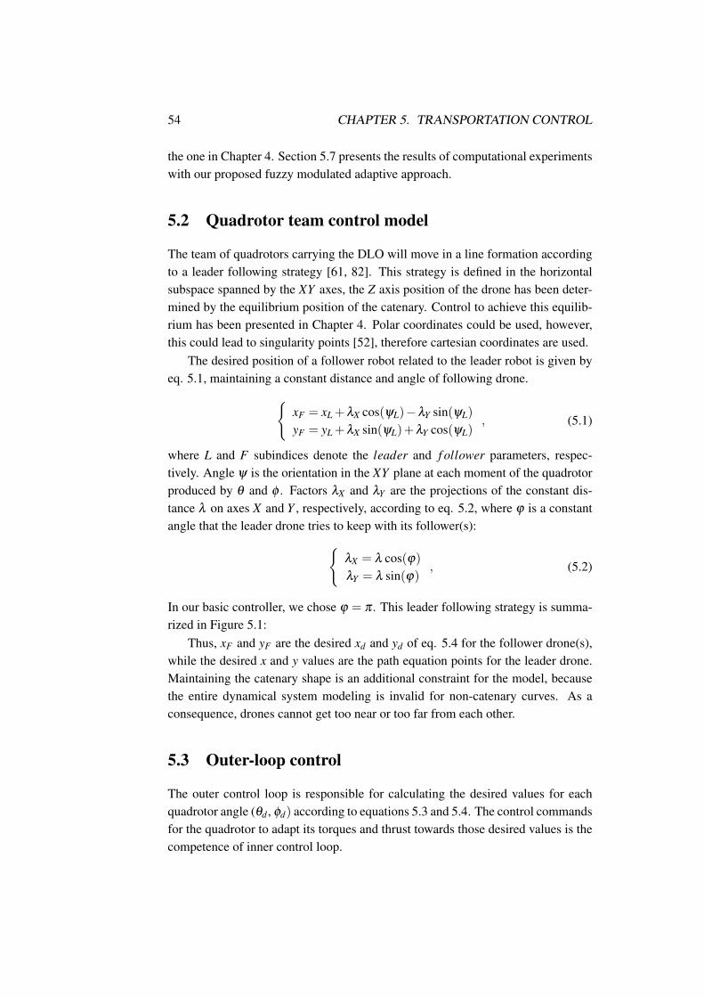
54 CHAPTER 5. TRANSPORTATION CONTROL
the one in Chapter 4. Section 5.7 presents the results of computational experimentswith our proposed fuzzy modulated adaptive approach.
5.2 Quadrotor team control model
The team of quadrotors carrying the DLO will move in a line formation accordingto a leader following strategy [61, 82]. This strategy is defined in the horizontalsubspace spanned by the XY axes, the Z axis position of the drone has been deter-mined by the equilibrium position of the catenary. Control to achieve this equilib-rium has been presented in Chapter 4. Polar coordinates could be used, however,this could lead to singularity points [52], therefore cartesian coordinates are used.
The desired position of a follower robot related to the leader robot is given byeq. 5.1, maintaining a constant distance and angle of following drone.
xF = xL +λX cos(ψL)−λY sin(ψL)
yF = yL +λX sin(ψL)+λY cos(ψL), (5.1)
where L and F subindices denote the leader and f ollower parameters, respec-tively. Angle ψ is the orientation in the XY plane at each moment of the quadrotorproduced by θ and φ . Factors λX and λY are the projections of the constant dis-tance λ on axes X and Y , respectively, according to eq. 5.2, where ϕ is a constantangle that the leader drone tries to keep with its follower(s):
λX = λ cos(ϕ)λY = λ sin(ϕ)
, (5.2)
In our basic controller, we chose ϕ = π . This leader following strategy is summa-rized in Figure 5.1:
Thus, xF and yF are the desired xd and yd of eq. 5.4 for the follower drone(s),while the desired x and y values are the path equation points for the leader drone.Maintaining the catenary shape is an additional constraint for the model, becausethe entire dynamical system modeling is invalid for non-catenary curves. As aconsequence, drones cannot get too near or too far from each other.
5.3 Outer-loop control
The outer control loop is responsible for calculating the desired values for eachquadrotor angle (θd , φd) according to equations 5.3 and 5.4. The control commandsfor the quadrotor to adapt its torques and thrust towards those desired values is thecompetence of inner control loop.
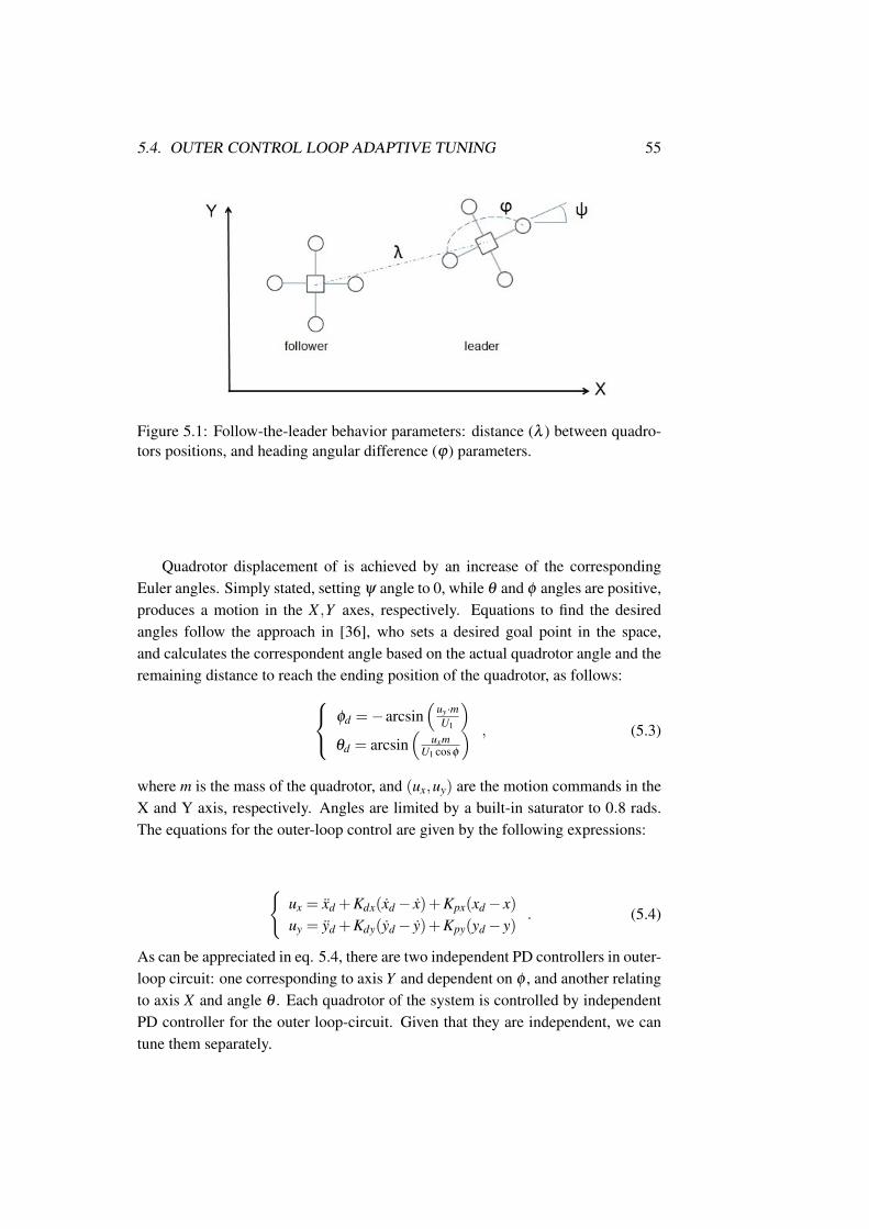
5.4. OUTER CONTROL LOOP ADAPTIVE TUNING 55
Figure 5.1: Follow-the-leader behavior parameters: distance (λ ) between quadro-tors positions, and heading angular difference (ϕ) parameters.
Quadrotor displacement of is achieved by an increase of the correspondingEuler angles. Simply stated, setting ψ angle to 0, while θ and φ angles are positive,produces a motion in the X ,Y axes, respectively. Equations to find the desiredangles follow the approach in [36], who sets a desired goal point in the space,and calculates the correspondent angle based on the actual quadrotor angle and theremaining distance to reach the ending position of the quadrotor, as follows: φd =−arcsin
(uy·mU1
)θd = arcsin
(uxm
U1 cosφ
) , (5.3)
where m is the mass of the quadrotor, and (ux,uy) are the motion commands in theX and Y axis, respectively. Angles are limited by a built-in saturator to 0.8 rads.The equations for the outer-loop control are given by the following expressions:
ux = xd +Kdx(xd− x)+Kpx(xd− x)uy = yd +Kdy(yd− y)+Kpy(yd− y)
. (5.4)
As can be appreciated in eq. 5.4, there are two independent PD controllers in outer-loop circuit: one corresponding to axis Y and dependent on φ , and another relatingto axis X and angle θ . Each quadrotor of the system is controlled by independentPD controller for the outer loop-circuit. Given that they are independent, we cantune them separately.
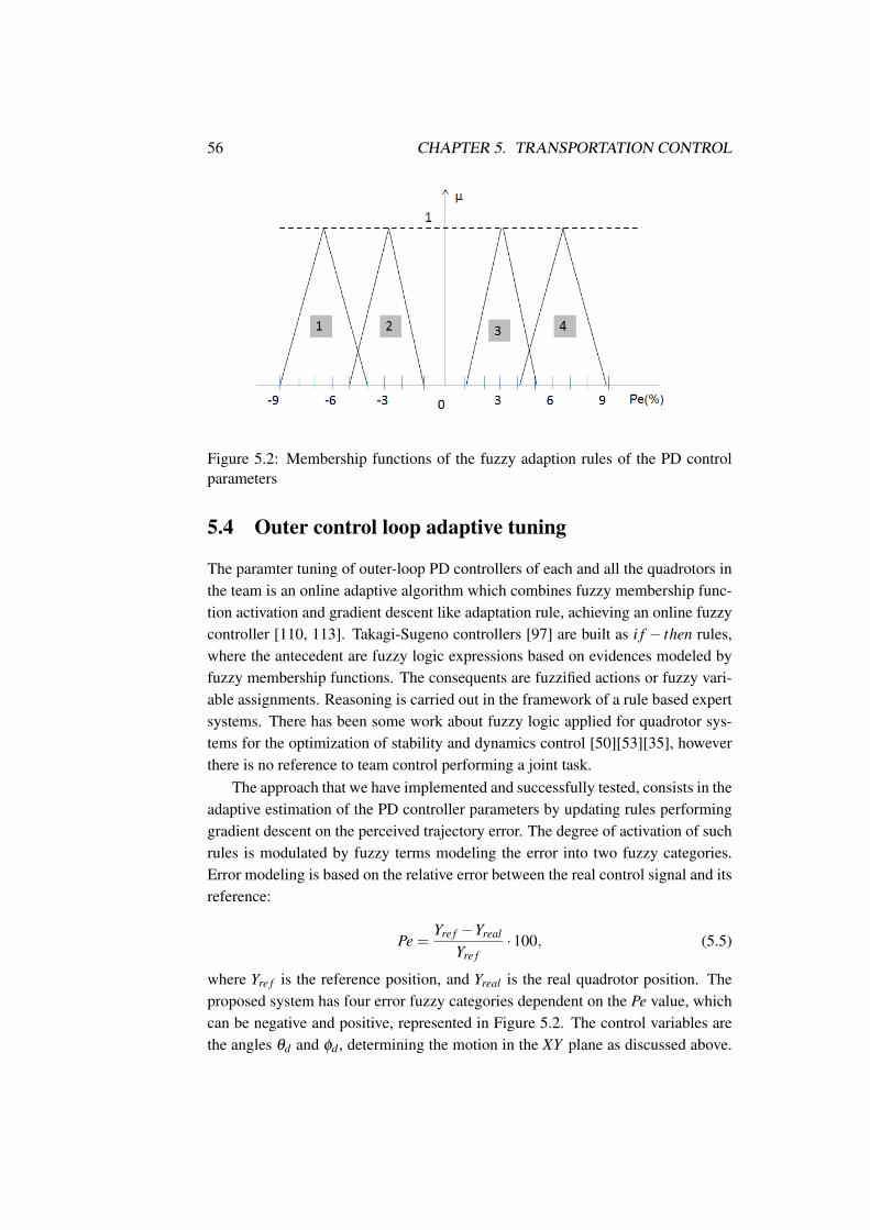
56 CHAPTER 5. TRANSPORTATION CONTROL
Figure 5.2: Membership functions of the fuzzy adaption rules of the PD controlparameters
5.4 Outer control loop adaptive tuning
The paramter tuning of outer-loop PD controllers of each and all the quadrotors inthe team is an online adaptive algorithm which combines fuzzy membership func-tion activation and gradient descent like adaptation rule, achieving an online fuzzycontroller [110, 113]. Takagi-Sugeno controllers [97] are built as i f − then rules,where the antecedent are fuzzy logic expressions based on evidences modeled byfuzzy membership functions. The consequents are fuzzified actions or fuzzy vari-able assignments. Reasoning is carried out in the framework of a rule based expertsystems. There has been some work about fuzzy logic applied for quadrotor sys-tems for the optimization of stability and dynamics control [50][53][35], howeverthere is no reference to team control performing a joint task.
The approach that we have implemented and successfully tested, consists in theadaptive estimation of the PD controller parameters by updating rules performinggradient descent on the perceived trajectory error. The degree of activation of suchrules is modulated by fuzzy terms modeling the error into two fuzzy categories.Error modeling is based on the relative error between the real control signal and itsreference:
Pe =Yre f −Yreal
Yre f·100, (5.5)
where Yre f is the reference position, and Yreal is the real quadrotor position. Theproposed system has four error fuzzy categories dependent on the Pe value, whichcan be negative and positive, represented in Figure 5.2. The control variables arethe angles θd and φd , determining the motion in the XY plane as discussed above.
5.4. OUTER CONTROL LOOP ADAPTIVE TUNING 57
We have a independent PD controller for each angle. Therefore, there are two errore(t) functions depending on the spatial coordinate to control, as shown in eq. 5.6:
eφ (t) = φd−φ (t)eθ (t) = θd−θ (t)
, (5.6)
where φd and θd are the desired values of the angles. Membership functionsµ1 (Pe(t)) and µ4 (Pe(t)) modulate the activation of equation 5.7 that performsthe adaptation of parameter Kp, while functions µ2 (Pe(t)) and µ3 (Pe(t)) modu-late the activation of equation 5.8 that performing the adaptation of parameter Kd .The online parameter adaptation equations read as follows:
Kp (t +1) = Kp (t)+αe(t)(µ1 (Pe(t))+µ4 (Pe(t))) (5.7)
Kd(t +1) = Kd (t)+αe(t)(µ2 (Pe(t))+µ3 (Pe(t))) (5.8)
where α is the adaptation factor, e(t) is the navigation error at each t moment, andµk (Pe(t)) is the k− th membership value function, which provides the activationstrength of the adaptation function (note that the activation values are always be-tween 0 and 1 due to the triangular shape of the membership functions specifiedin Figure 5.2, which have empty support intersections). The adaption factor α isinitialized with a value between 0 and 1 and remains constant until the end of theprocess. The online PD controller tuning is intended to allow the system to adapt todifferent trajectories, dynamic parameters of the quadrotors, and unknown catenaryweight per length.
Convergence of the fuzzy modulation approach The online adaptation equa-tions Eq. (5.7) and Eq. (5.8) are in fact instances of the general stochastic gradientdescent algorithm applied in many neural network learning algorithms. It is wellknown that convergence of online stochastic gradient descent learning in station-ary environments require that the gradient descent gain αt complies with conditions∑t α2
t < ∞ and limt→∞
αt = 0. However, if the environment is non-stationary the decayof the gradient descent gain freezes adaptation, so that after some time the systembecomes insensitive to changes in the environment and, therefore, equivalent to anoffline training/tuning algorithm. Hence we leave the gain fixed to a small constantvalue, so that adaptation is never stopped. Additionally, the membership functionmodulation factors further enhance convergence, because they focus the learning ofthe PID coefficients Kp and Kd according to the error magnitude. For greater errormagnitude, the Kp coefficient is more affected, while fine tuning to small errors isachieved affecting the Kd coefficient. Lacking a formal analytical proof, the intu-

58 CHAPTER 5. TRANSPORTATION CONTROL
ition is that the process will not diverge because the overall gain is always smallerthan 1. Empirical (simulated) experiments confirm that the approach works well.
5.5 Heuristics for smooth behaviors
In a multi-quadrotor system, there is no gurantee that all the robots will fly at thesame speed, therefore inducing distance variations among catenary nodes, whichmay lead to system instability and collapse. In order to prevent that, two extraconditions are introduced in the model. For each leader-follower pair of drones:
• If the euclidean distance between drones overcomes a threshold, the leader’sdesired angles turn to 0 until the distance falls within the desired range again.
• If the euclidean distance between drones is shorter than a threshold, the fol-lower’s desired angles turn to 0 until the distance increases.
Besides, ϕ constant angle creates sharp path changes, and abrupt changes in cate-nary node distances. To achieve path smoothing we make ϕ variable, as follows:
ϕ = π− (ψL−ψF)
2, (5.9)
where, ψL and ψF are the XY heading angles of the leader and follower robotrespectively, in [rad].
5.6 Experiment 2
This section gives results on the baseline PD controller tuning by a PSO approachfor the DLO transportation task, as in the tuning of the controller to achieve theequi-workload position in Chapter 4. We train a PD controller, which is applied toeach of the four rotors in the quadrotor. The PSO cost function value is computedafter the simulation of the system performing one instance of the task. There-fore, carrying the PD parameter tuning by PSO is very time consuming, involvingthousands of simulations. Once the PD parameter values are chosen, robustnessexperiments are carried out.
The experimental system is composed of three quadrotors carrying a DLO intwo sections of symmetric catenaries, with the robots flying in parallel. That is,three quadrotors must reach the (x0,i +∆x,y0,i +∆y) coordinates at the same time,where (x0,i,y0,i) is the inital position of the i-th robot, and (x,y) is the displacementto the desired position. Robots are named D1, D2, and D3.
Time increment used to compute simulation steps is 0.1 seconds. Specific val-ues of system parameters in the experiment are: each catenary section has length
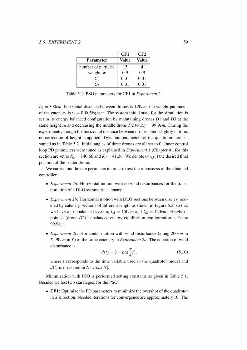
5.6. EXPERIMENT 2 59
CF1 CF2Parameter Value Value
number of particles 15 4weight, w 0.9 0.9
C1 0.01 0.01C2 0.01 0.01
Table 5.1: PSO parameters for CF1 in Experiment 2
L0 = 300cm; horizontal distance between drones is 120cm, the weight parameterof the catenary is w = 0,005kg/cm. The system initial state for the simulation isset in its energy balanced configuration by maintaining drones D1 and D3 at thesame height z0 and decreasing the middle drone D2 to 4y = 99.9cm. During theexperiments, though the horizontal distance between drones alters slightly in time,no correction of height is applied. Dynamic parameters of the quadrotors are as-sumed as in Table 5.2. Initial angles of three drones are all set to 0. Inner controlloop PD parameters were tuned as explained in Experiment 1 (Chapter 4), for thissection are set to Kp = 140.66 and Kd = 41.36. We denote (xd ,yd) the desired finalposition of the leader drone.
We carried out three experiments in order to test the robustness of the obtainedcontroller.
• Experiment 2a: Horizontal motion with no wind disturbances for the trans-portation of a DLO symmetric catenary.
• Experiment 2b: Horizontal motion with DLO sections between drones mod-eled by catenary sections of different length as shown in Figure 5.3, so thatwe have an unbalanced system, lx1 = 150cm and lx2 = 120cm. Height ofpoint A (drone D2) at balanced energy equilibrium configuration is 4y =
99.9cm.
• Experiment 2c: Horizontal motion with wind disturbance (along 200cm inX , 90cm in Y ) of the same catenary in Experiment 2a. The equation of winddisturbance is:
d(t) = 3+ sin(π
4t), (5.10)
where t corresponds to the time variable used in the quadrotor model andd(t) is measured in Newtons[N].
Minimization with PSO is performed setting constants as given in Table 5.1.Besides we test two starategies for the PSO:
• CF1: Optimize the PD parameters to minimize the overshot of the quadrotorin X direction. Needed iterations for convergence are approximately 10. The
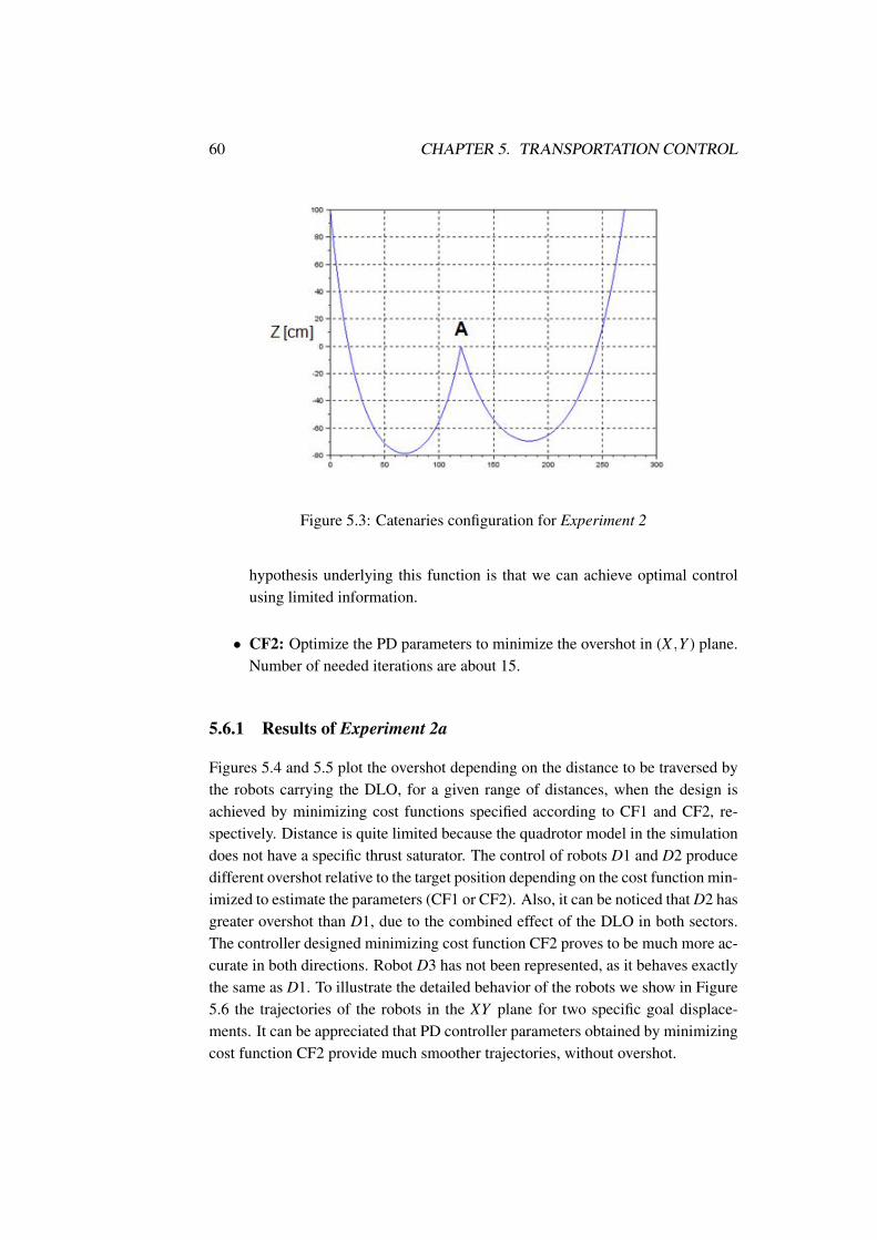
60 CHAPTER 5. TRANSPORTATION CONTROL
Figure 5.3: Catenaries configuration for Experiment 2
hypothesis underlying this function is that we can achieve optimal controlusing limited information.
• CF2: Optimize the PD parameters to minimize the overshot in (X ,Y ) plane.Number of needed iterations are about 15.
5.6.1 Results of Experiment 2a
Figures 5.4 and 5.5 plot the overshot depending on the distance to be traversed bythe robots carrying the DLO, for a given range of distances, when the design isachieved by minimizing cost functions specified according to CF1 and CF2, re-spectively. Distance is quite limited because the quadrotor model in the simulationdoes not have a specific thrust saturator. The control of robots D1 and D2 producedifferent overshot relative to the target position depending on the cost function min-imized to estimate the parameters (CF1 or CF2). Also, it can be noticed that D2 hasgreater overshot than D1, due to the combined effect of the DLO in both sectors.The controller designed minimizing cost function CF2 proves to be much more ac-curate in both directions. Robot D3 has not been represented, as it behaves exactlythe same as D1. To illustrate the detailed behavior of the robots we show in Figure5.6 the trajectories of the robots in the XY plane for two specific goal displace-ments. It can be appreciated that PD controller parameters obtained by minimizingcost function CF2 provide much smoother trajectories, without overshot.
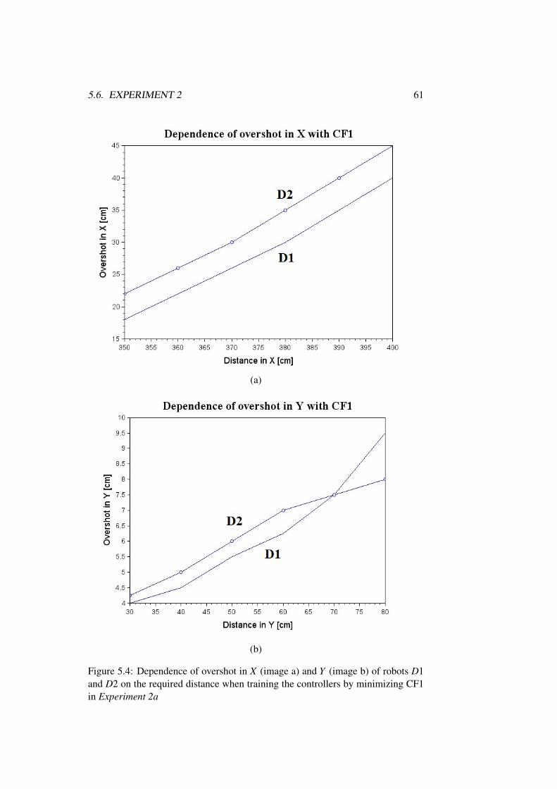
5.6. EXPERIMENT 2 61
(a)
(b)
Figure 5.4: Dependence of overshot in X (image a) and Y (image b) of robots D1and D2 on the required distance when training the controllers by minimizing CF1in Experiment 2a
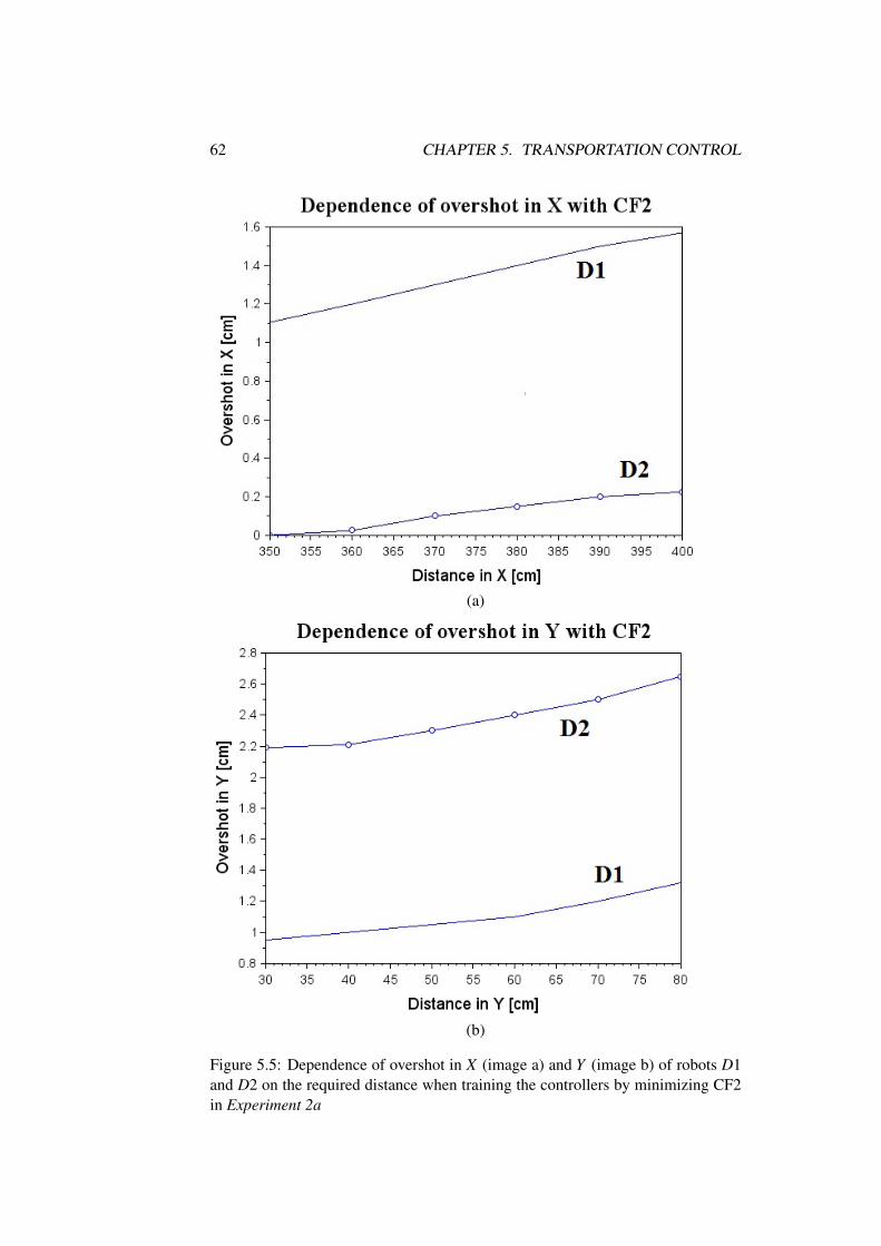
62 CHAPTER 5. TRANSPORTATION CONTROL
(a)
(b)
Figure 5.5: Dependence of overshot in X (image a) and Y (image b) of robots D1and D2 on the required distance when training the controllers by minimizing CF2in Experiment 2a
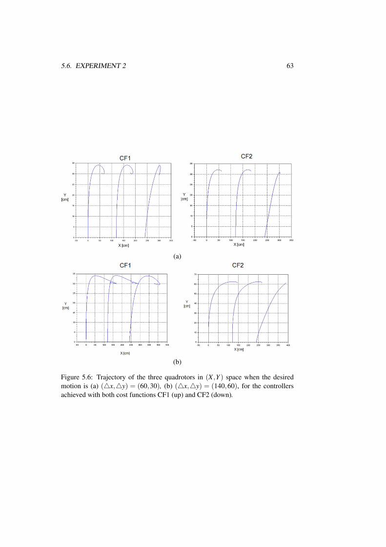
5.6. EXPERIMENT 2 63
(a)
(b)
Figure 5.6: Trajectory of the three quadrotors in (X ,Y ) space when the desiredmotion is (a) (4x,4y) = (60,30), (b) (4x,4y) = (140,60), for the controllersachieved with both cost functions CF1 (up) and CF2 (down).
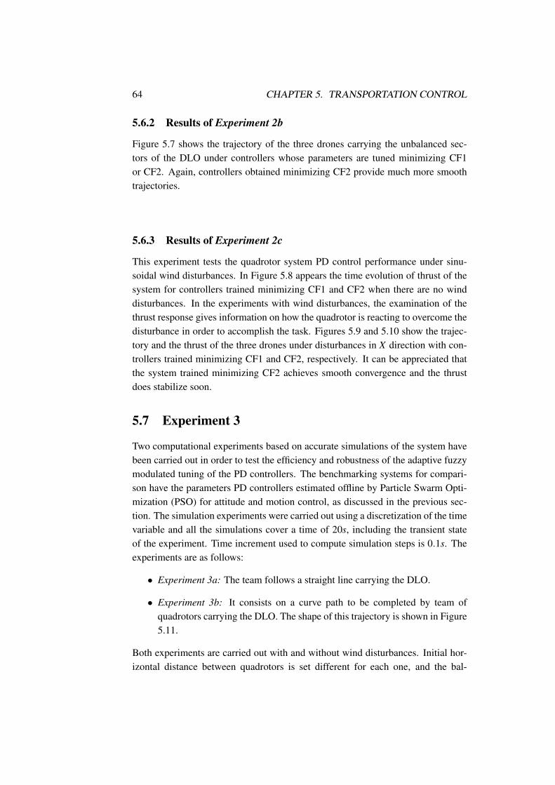
64 CHAPTER 5. TRANSPORTATION CONTROL
5.6.2 Results of Experiment 2b
Figure 5.7 shows the trajectory of the three drones carrying the unbalanced sec-tors of the DLO under controllers whose parameters are tuned minimizing CF1or CF2. Again, controllers obtained minimizing CF2 provide much more smoothtrajectories.
5.6.3 Results of Experiment 2c
This experiment tests the quadrotor system PD control performance under sinu-soidal wind disturbances. In Figure 5.8 appears the time evolution of thrust of thesystem for controllers trained minimizing CF1 and CF2 when there are no winddisturbances. In the experiments with wind disturbances, the examination of thethrust response gives information on how the quadrotor is reacting to overcome thedisturbance in order to accomplish the task. Figures 5.9 and 5.10 show the trajec-tory and the thrust of the three drones under disturbances in X direction with con-trollers trained minimizing CF1 and CF2, respectively. It can be appreciated thatthe system trained minimizing CF2 achieves smooth convergence and the thrustdoes stabilize soon.
5.7 Experiment 3
Two computational experiments based on accurate simulations of the system havebeen carried out in order to test the efficiency and robustness of the adaptive fuzzymodulated tuning of the PD controllers. The benchmarking systems for compari-son have the parameters PD controllers estimated offline by Particle Swarm Opti-mization (PSO) for attitude and motion control, as discussed in the previous sec-tion. The simulation experiments were carried out using a discretization of the timevariable and all the simulations cover a time of 20s, including the transient stateof the experiment. Time increment used to compute simulation steps is 0.1s. Theexperiments are as follows:
• Experiment 3a: The team follows a straight line carrying the DLO.
• Experiment 3b: It consists on a curve path to be completed by team ofquadrotors carrying the DLO. The shape of this trajectory is shown in Figure5.11.
Both experiments are carried out with and without wind disturbances. Initial hor-izontal distance between quadrotors is set different for each one, and the bal-
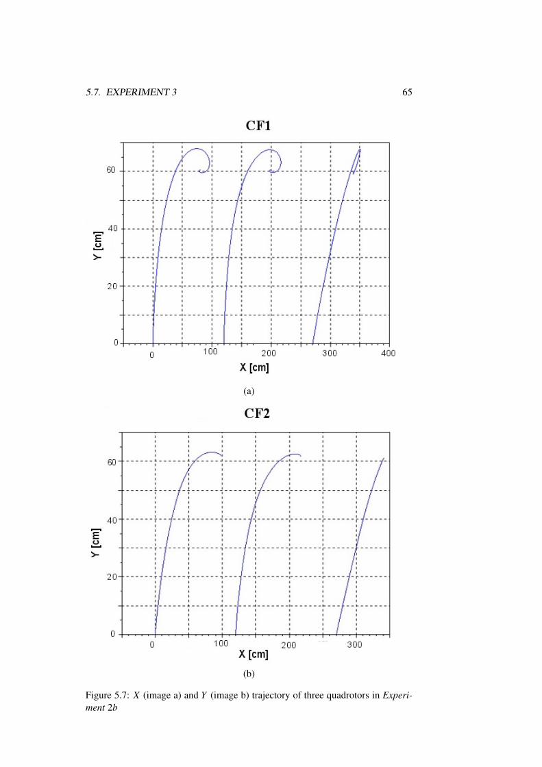
5.7. EXPERIMENT 3 65
(a)
(b)
Figure 5.7: X (image a) and Y (image b) trajectory of three quadrotors in Experi-ment 2b
66 CHAPTER 5. TRANSPORTATION CONTROL
(a)
(b)
Figure 5.8: Thrust of D1 and D2 in Experiment 2c under no disturbances
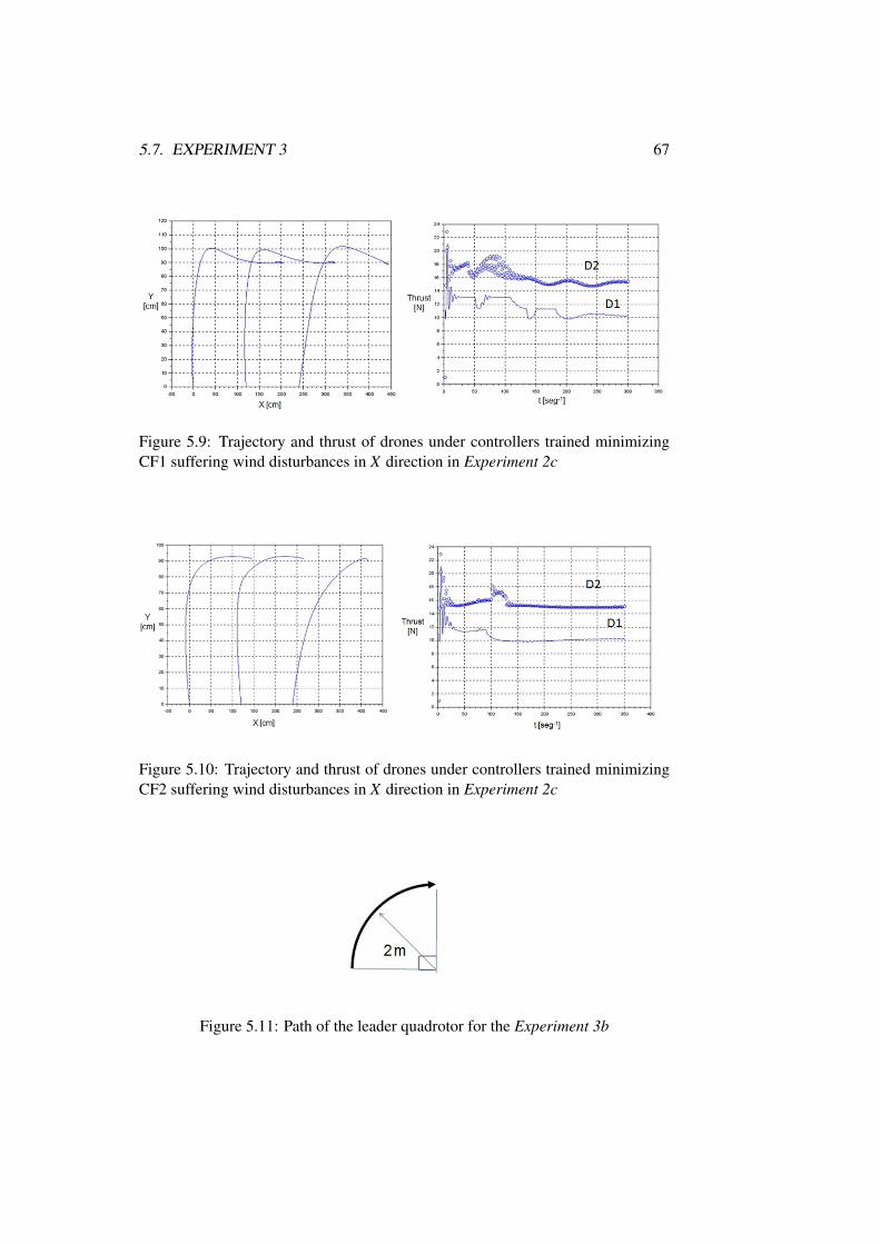
5.7. EXPERIMENT 3 67
Figure 5.9: Trajectory and thrust of drones under controllers trained minimizingCF1 suffering wind disturbances in X direction in Experiment 2c
Figure 5.10: Trajectory and thrust of drones under controllers trained minimizingCF2 suffering wind disturbances in X direction in Experiment 2c
Figure 5.11: Path of the leader quadrotor for the Experiment 3b
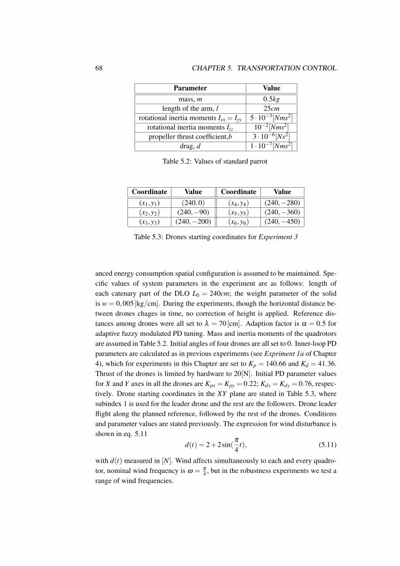
68 CHAPTER 5. TRANSPORTATION CONTROL
Parameter Valuemass, m 0.5kg
length of the arm, l 25cmrotational inertia moments Ixx = Iyy 5 ·10−3[Nms2]
rotational inertia moments Izz 10−2[Nms2]
propeller thrust coefficient,b 3 ·10−6[Ns2]
drag, d 1 ·10−7[Nms2]
Table 5.2: Values of standard parrot
Coordinate Value Coordinate Value(x1,y1) (240,0) (x4,y4) (240,−280)(x2,y2) (240,−90) (x5,y5) (240,−360)(x3,y3) (240,−200) (x6,y6) (240,−450)
Table 5.3: Drones starting coordinates for Experiment 3
anced energy consumption spatial configuration is assumed to be maintained. Spe-cific values of system parameters in the experiment are as follows: length ofeach catenary part of the DLO L0 = 240cm; the weight parameter of the solidis w = 0,005 [kg/cm]. During the experiments, though the horizontal distance be-tween drones chages in time, no correction of height is applied. Reference dis-tances among drones were all set to λ = 70 [cm]. Adaption factor is α = 0.5 foradaptive fuzzy modulated PD tuning. Mass and inertia moments of the quadrotorsare assumed in Table 5.2. Initial angles of four drones are all set to 0. Inner-loop PDparameters are calculated as in previous experiments (see Expriment 1a of Chapter4), which for experiments in this Chapter are set to Kp = 140.66 and Kd = 41.36.Thrust of the drones is limited by hardware to 20[N]. Initial PD parameter valuesfor X and Y axes in all the drones are Kpx = Kpy = 0.22; Kdx = Kdy = 0.76, respec-tively. Drone starting coordinates in the XY plane are stated in Table 5.3, wheresubindex 1 is used for the leader drone and the rest are the followers. Drone leaderflight along the planned reference, followed by the rest of the drones. Conditionsand parameter values are stated previously. The expression for wind disturbance isshown in eq. 5.11
d(t) = 2+2sin(π
4t), (5.11)
with d(t) measured in [N]. Wind affects simultaneously to each and every quadro-tor, nominal wind frequency is ω = π
4 , but in the robustness experiments we test arange of wind frequencies.
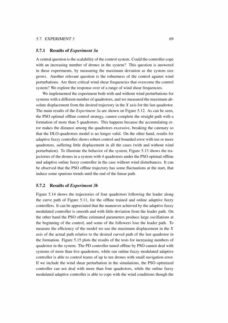
5.7. EXPERIMENT 3 69
5.7.1 Results of Experiment 3a
A central question is the scalability of the control system. Could the controller copewith an increasing number of drones in the system? This question is answeredin these experiments, by measuring the maximum deviation as the system sizegrows. Another relevant question is the robustness of the control against windperturbations. Are there critical wind shear frequencies that overcome the controlsystem? We explore the response over of a range of wind shear frequencies.
We implemented the experiment both with and without wind perturbations forsystems with a different number of quadrotors, and we measured the maximum ab-solute displacement from the desired trajectory in the X axis for the last quadrotor.The main results of the Experiment 3a are shown on Figure 5.12. As can be seen,the PSO optimal offline control strategy, cannot complete the straight path with aformation of more than 5 quadrotors. This happens because the accumulating er-ror makes the distance among the quadrotors excessive, breaking the catenary sothat the DLO-quadrotors model is no longer valid. On the other hand, results foradaptive fuzzy controller shows robust control and bounded error with ten or morequadrotors, suffering little displacement in all the cases (with and without windperturbation). To illustrate the behavior of the system, Figure 5.13 shows the tra-jectories of the drones in a system with 4 quadrotors under the PSO optimal offlineand adaptive online fuzzy controller in the case without wind disturbances. It canbe observed that the PSO offline trajectory has some fluctuations at the start, thatinduce some spurious trends until the end of the linear path.
5.7.2 Results of Experiment 3b
Figure 5.14 shows the trajectories of four quadrotors following the leader alongthe curve path of Figure 5.11, for the offline trained and online adaptive fuzzycontrollers. It can be appreciated that the maneuver achieved by the adaptive fuzzymodulated controller is smooth and with little deviation from the leader path. Onthe other hand the PSO offline estimated parameters produce large oscillations atthe beginning of the control, and some of the followers lose the leader path. Tomeasure the efficiency of the model we use the maximum displacement in the Xaxis of the actual path relative to the desired curved path of the last quadrotor inthe formation. Figure 5.15 plots the results of the tests for increasing numbers ofquadrotor in the system. The PD controller tuned offline by PSO cannot deal withsystems of more than five quadrotors, while our online fuzzy modulated adaptivecontroller is able to control teams of up to ten drones with small navigation error.If we include the wind shear perturbation in the simulations, the PSO optimizedcontroller can not deal with more than four quadrotors, while the online fuzzymodulated adaptive controller is able to cope with the wind conditions though the
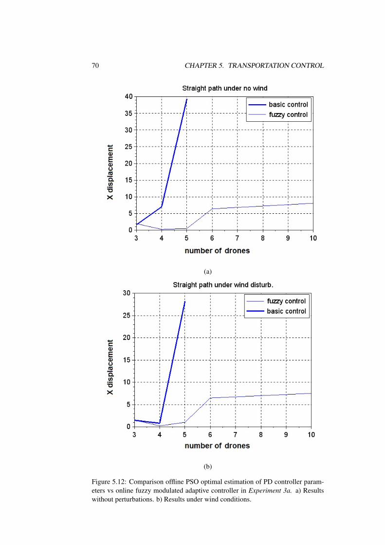
70 CHAPTER 5. TRANSPORTATION CONTROL
(a)
(b)
Figure 5.12: Comparison offline PSO optimal estimation of PD controller param-eters vs online fuzzy modulated adaptive controller in Experiment 3a. a) Resultswithout perturbations. b) Results under wind conditions.
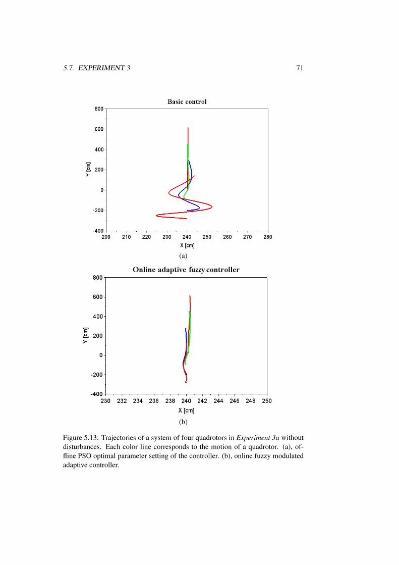
5.7. EXPERIMENT 3 71
(a)
(b)
Figure 5.13: Trajectories of a system of four quadrotors in Experiment 3a withoutdisturbances. Each color line corresponds to the motion of a quadrotor. (a), of-fline PSO optimal parameter setting of the controller. (b), online fuzzy modulatedadaptive controller.
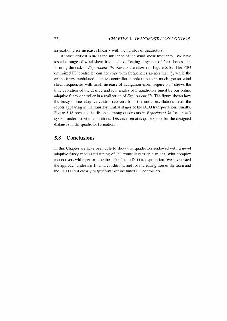
72 CHAPTER 5. TRANSPORTATION CONTROL
navigation error increases linearly with the number of quadrotors.Another critical issue is the influence of the wind shear frequency. We have
tested a range of wind shear frequencies affecting a system of four drones per-forming the task of Experiment 3b. Results are shown in Figure 5.16. The PSOoptimized PD controller can not cope with frequencies greater than π
2 , while theonline fuzzy modulated adaptive controller is able to sustain much greater windshear frequencies with small increase of navigation error. Figure 5.17 shows thetime evolution of the desired and real angles of 3 quadrotors tuned by our onlineadaptive fuzzy controller in a realization of Experiment 3b. The figure shows howthe fuzzy online adaptive control recovers from the initial oscillations in all therobots appearing in the transitory initial stages of the DLO transportation. Finally,Figure 5.18 presents the distance among quadrotors in Experiment 3b for a n = 3system under no wind conditions. Distance remains quite stable for the designeddistances in the quadrotor formation.
5.8 Conclusions
In this Chapter we have been able to show that quadrotors endowed with a noveladaptive fuzzy modulated tuning of PD controllers is able to deal with complexmaneouvers while performing the task of team DLO transportation. We have testedthe approach under harsh wind conditions, and for increasing size of the team andthe DLO and it clearly outperforms offline tuned PD controllers.
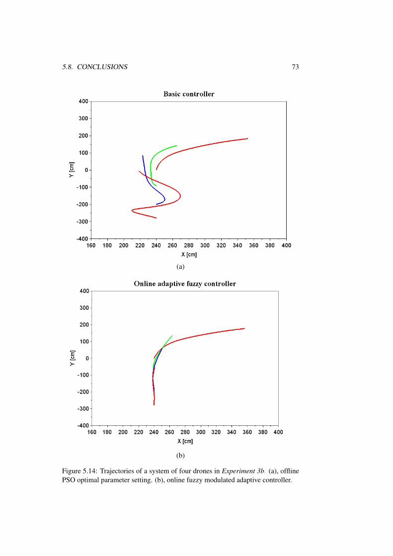
5.8. CONCLUSIONS 73
(a)
(b)
Figure 5.14: Trajectories of a system of four drones in Experiment 3b. (a), offlinePSO optimal parameter setting. (b), online fuzzy modulated adaptive controller.
74 CHAPTER 5. TRANSPORTATION CONTROL
(a)
(b)
Figure 5.15: Error of offline PSO optimal parameter setting versus online fuzzymodulated adaptive controller following a curve path in Experiment 3b, increasingthe number of quadrotors in the system. a) plot without wind shear infuence. b)wind frequency perturbation is set to its nominal value.
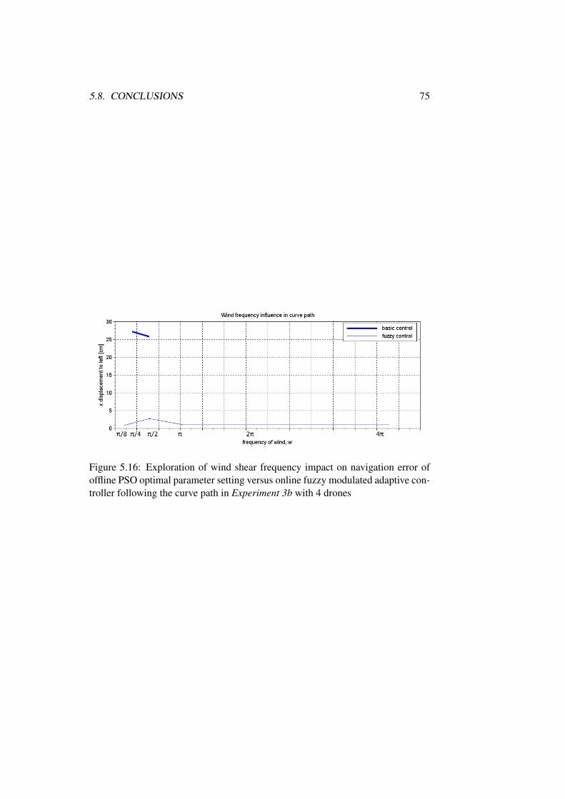
5.8. CONCLUSIONS 75
Figure 5.16: Exploration of wind shear frequency impact on navigation error ofoffline PSO optimal parameter setting versus online fuzzy modulated adaptive con-troller following the curve path in Experiment 3b with 4 drones
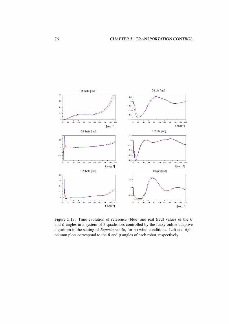
76 CHAPTER 5. TRANSPORTATION CONTROL
Figure 5.17: Time evolution of reference (blue) and real (red) values of the θ
and φ angles in a system of 3 quadrotors controlled by the fuzzy online adaptivealgorithm in the setting of Experiment 3b, for no wind conditions. Left and rightcolumn plots correspond to the θ and φ angles of each robot, respectively.
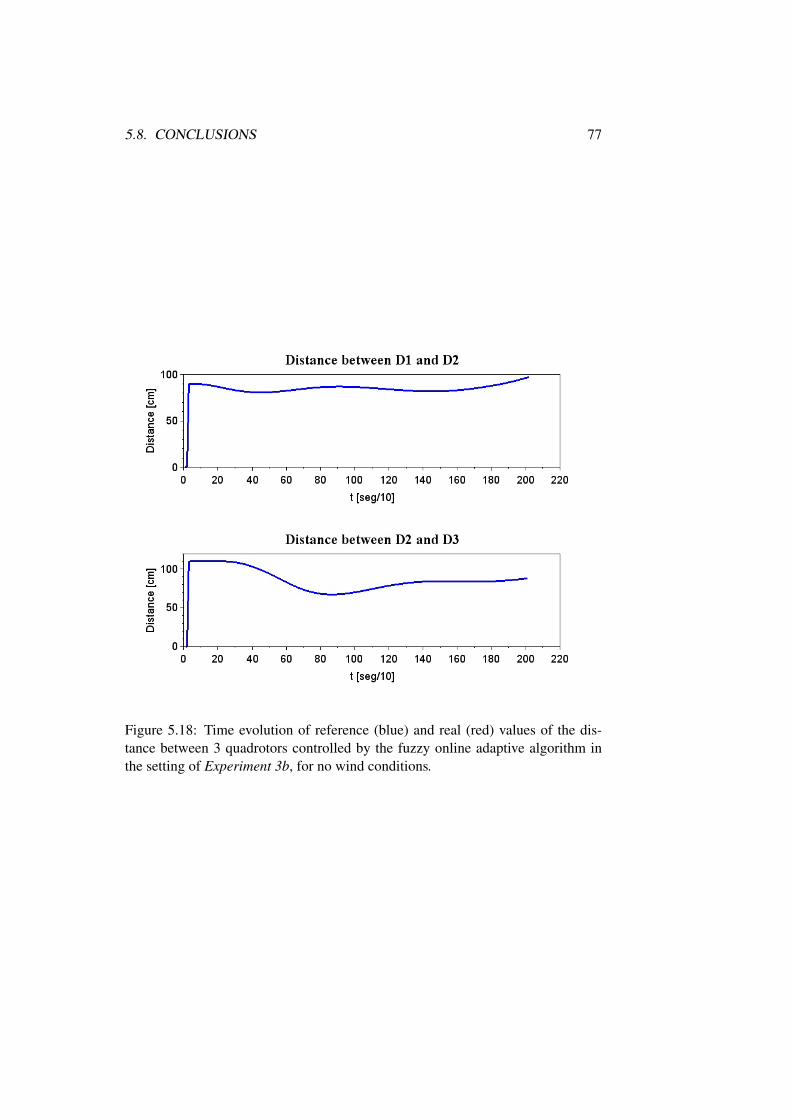
5.8. CONCLUSIONS 77
Figure 5.18: Time evolution of reference (blue) and real (red) values of the dis-tance between 3 quadrotors controlled by the fuzzy online adaptive algorithm inthe setting of Experiment 3b, for no wind conditions.

78 CHAPTER 5. TRANSPORTATION CONTROL
Chapter 6
Conclusions and Future Work
6.1 Conclusions
The general goals of the Thesis were proposed in the Introduction. Sections 6.1.1,6.1.2and 6.1.3 discuss our achievements of these goals.
6.1.1 Aerial robots modeling for cooperative transportation of DLOs
In this Thesis a novel model of a system to transport DLO solids such as wires andropes with some aerial robots has been proposed and validated and it represents awork aligned with the Linked Multi-Robot-Component-Systems that the researchgroup of Computational Intelligence in UPV-EHU previously worked on. Being aquadrotor a non-linear system, a careful and precise modeling becomes indispens-able. In our approach, the dofs of the system are related to body-centered frameangles (yaw, pitch, roll) and earth-frame Z coordinate. The proposal presents anovel way of representing DLO during transportation as catenaries, going a stepfurther of the state of the art, as most researchers consider payload transportationwith UAVs modelled as a pendulum. The dynamic parameters used for the experi-ments are standard drones’ and do not require any modification excepting the ideallinking point between the catenary and the UAV. The simulations show feasibledrone behaviour and torque-thrust values.
6.1.2 Offline control strategy
Each quadrotor control was formed by two-loops circuits: attitude-control (inner-loop) and position-control circuits (outer-loop). We considered that all the quadro-tors share the same values of inner controllers and that all the circuits related to thefour dofs are equal. Offline control strategy was used in first phase for inner-looptuning and in second, for outer-loop tuning.
79
80 CHAPTER 6. CONCLUSIONS AND FUTURE WORK
We have compared two PID/PD offline tuning methods to adapt the quadro-tor system for a smooth, fast and reliable behaviour. Firstly, we tested classicalZiegler-Nichols strategy, and later, we adopted an intelligent tuning method: PSO(Particle Swarm Optimization). Results showed that PSO tuning obtained a betterperformance, which also resulted to be robust to different quadrotor dynamic pa-rameters and different catenary own weights, which turn the transportation systeminto an adaptable and robust system and PSO implementation showed good resultseven with only PD parameters. These experiments were carried out in a single axisdirection.
In the second phase of the offline control tuning, horizontal motion of quadro-tor system was implemented. Here, only PSO tuning was tested under differentstress conditions, paths distances and catenary weights. Experiments resulted in abetter performance of the UAV systems if the PSO tuning considered two movingdirections rather than only one.
6.1.3 Online adaptive control strategy
Online adaptive strategy was applied to outer-loop PD tuning only. We consid-ered inner-loop PD values fixed by PSO in previous step. An adaptive fuzzystrategy tuning method was implemented, inspired on Takagi-Sugeno controllersand i f − then rules. This tuning strategy was tested in linear and curve paths forquadrotor transportation systems against basic offline control based on PSO algo-rithm. Effects of number of drone members was also studied and experiments werecarried out under different stress conditions.
Besides, a proposal of quadrotors formation both in curve and straight pathswas proposed, considering the distance constraints that catenary usage implies.
6.2 Future Work
Next, Sections 6.2.1, 6.2.2 describe the future work plan for the three main areasshown in this Thesis.
6.2.1 System modeling
Further work will involve testing new approaches to cope with transient states pro-voked by DLOs and their deformation during transportation process. As explainedin State of Art Chapter, multiple proposals of deformable linear objects exist, buta further study on how these dynamic effects change the quadrotor transportationcurrent behaviour should be studied.
6.2. FUTURE WORK 81
Moreover, an experimental realization of the quadrotor DLOs transporting sys-tem is highly advisable in order to test the efectiveness and eficiency of currentThesis work. This step will drop loads of information about correct solids or per-turbations modeling, control strategy and extra features.
Collision with ground surfaces render the catenary model inaccurate and theyhappen in the phases of take off and landing. In this Thesis work have not beentaken into consideration, and thus and enhancement of the model to adopt thisposibility appears as a challenging task.
6.2.2 Control strategy
Implementation of Machine Learning Techniques to our system, focused on futureimplementation of professional routine works, such as the continuous transporta-tion of cables from one point to another. We refer to adaptive systems when thesystem uses some intelligent algorithms to find the most suitable actions to its cur-rent situation, but we talk about "learning" machine or system once the systemis not just able to find some efficient solutions by running some intelligent meth-ods, but also through memorizing, comparing the result of "adaptive" algorithm.Sort of getting experience with time. Machine learning presents a wide horizon ofpossibilities to implement in drone applications such this.
82 CHAPTER 6. CONCLUSIONS AND FUTURE WORK
Bibliography
[1] K. J. AAström and T. Hägglund. PID Controllers: Theory, Design, andTuning. Instrument Society of America, Research Triangle Park, NC, 2edition, 1995.
[2] J. Acker and D. Henrich. Manipulation of deformable linear objects: Fromgeometric model towards program generation. In Robotics and Automation,2005. ICRA 2005. Proceedings of the 2005 IEEE International Conferenceon, pages 1541–1547, April 2005.
[3] Ramzy S. Ali, Ammar A. Aldair, and Ali K. Almousawi. Article: Design anoptimal pid controller using artificial bee colony and genetic algorithm forautonomous mobile robot. International Journal of Computer Applications,100(16):8–16, August 2014. Full text available.
[4] A. Andreu, L. Gil, and P. Roca. A new deformable catenary element for theanalysis of cable net structures. Computers & Structures, 84(29-30):1882–1890, Nov 2006.
[5] K.H. Ang, G.C.Y. Chong, and Y. Li. Pid control system analysis, design,and technology. IEEE Trans Control Systems Tech, 13(4):559–576, 2005.
[6] L.M. Argentim, W.C. Rezende, P.E. Santos, and R.A. Aguiar. Pid, lqr andlqr-pid on a quadcopter platform. In Informatics, Electronics Vision (ICIEV),2013 International Conference on, pages 1–6, May 2013.
[7] H. Asama, A. Matsumoto, and Y. Ishida. Design of an autonomous anddistributed robot system: Actress. In Intelligent Robots and Systems ’89. TheAutonomous Mobile Robots and Its Applications. IROS ’89. Proceedings.,IEEE/RSJ International Workshop on, pages 283–290, Sep 1989.
[8] F. Augugliaro, S. Lupashin, M. Hamer, C. Male, M. Hehn, M.W. Mueller,J.S. Willmann, F. Gramazio, M. Kohler, and R. D’Andrea. The flight as-sembled architecture installation: Cooperative construction with flying ma-chines. Control Systems, IEEE, 34(4):46–64, Aug 2014.
83
84 BIBLIOGRAPHY
[9] F. Augugliaro, A. Mirjan, F. Gramazio, M. Kohler, and R. D’Andrea. Build-ing tensile structures with flying machines. In Intelligent Robots and Sys-tems (IROS), 2013 IEEE/RSJ International Conference on, pages 3487–3492, Nov 2013.
[10] N. Barakat and R. Rajagopalan. Speed control of a dc motor using a feedfor-ward computed torque control scheme. In Intelligent Control, 1996., Pro-ceedings of the 1996 IEEE International Symposium on, pages 432–437,Sep 1996.
[11] G. Beni. The concept of cellular robotic system. In Intelligent Control,1988. Proceedings., IEEE International Symposium on, pages 57–62, Aug1988.
[12] A. H. Bond and L. Gasse. Front matter. In Alan H. BondLes Gasser, editor,Readings in Distributed Artificial Intelligence, pages iii –. Morgan Kauf-mann, 1988.
[13] John M. Borky. Payload technologies and applications for uninhabited airvehicles (uavs). In Aerospace Conference, 1997. Proceedings., IEEE, vol-ume 3, pages 267–283 vol.3, Feb 1997.
[14] Samir Bouabdallah, Roland Siegwart, Autonomous Systems, and Lab. Fullcontrol of a quadrotor. 2003.
[15] S. Labiod Boubertakh, S. Bencharef. Pso-based pid and control design andfor the stabilization and of a quadrotor. IEEE.
[16] Gordon Bowden. Stretched Wire Mechanics. eConf, C04100411:038, 2004.
[17] Tammaso Bresciani. Modelling, identification and control of a quadrotorhelicopter. Master’s Thesis ISRN LUTFD2/TFRT--5823--SE, Departmentof Automatic Control, Lund University, Sweden, October 2008.
[18] Joel Brown, Jean-Claude Latombe, and Kevin Montgomery. Real-time knot-tying simulation. The Visual Computer, 20(2):165–179, 2004.
[19] R.E. Brown, G.N. Maliotis, and J.A. Gibby. Pid self-tuning controllerfor aluminum rolling mill. Industry Applications, IEEE Transactions on,29(3):578–583, May 1993.
[20] P. Caloud, Wonyun Choi, J.-C. Latombe, C. Le Pape, and M. Yim. Indoorautomation with many mobile robots. In Intelligent Robots and Systems ’90.’Towards a New Frontier of Applications’, Proceedings. IROS ’90. IEEEInternational Workshop on, pages 67–72 vol.1, Jul 1990.

BIBLIOGRAPHY 85
[21] Y.U. Cao, A.S. Fukunaga, A.B. Kahng, and F. Meng. Cooperative mo-bile robotics: antecedents and directions. In Intelligent Robots and Systems95. ’Human Robot Interaction and Cooperative Robots’, Proceedings. 1995IEEE/RSJ International Conference on, volume 1, pages 226–234 vol.1,Aug 1995.
[22] T.-O. Chan and D. D. Lichti. 3d catenary curve fitting for geometric calibra-tion. ISPRS - International Archives of the Photogrammetry, Remote Sens-ing and Spatial Information Sciences, XXXVIII-5/W12:259–264, 2011.
[23] Peng Cheng, Jonathan Fink, Soonkyum Kim, and Vijay Kumar. Algorith-mic Foundation of Robotics VIII: Selected Contributions of the Eight In-ternational Workshop on the Algorithmic Foundations of Robotics, chapterCooperative Towing with Multiple Robots, pages 101–116. Springer BerlinHeidelberg, Berlin, Heidelberg, 2010.
[24] Shicong Dai, Taeyoung Lee, and Dennis S. Bernstein. Adaptive control ofa quadrotor uav transporting a cable-suspended load with unknown mass.In 53rd IEEE Conference on Decision and Control December 15-17, 2014.Los Angeles, California, USA. IEEE, 2014.
[25] G.G. Denisov, V.V. Novilov, and M.L. Smirnova. The momentum of wavesand their effect on the motion of lumped objects along one-dimensional elas-tic systems. Journal of Applied Mathematics and Mechanics, 76(2):225 –234, 2012.
[26] T. Dierks and S. Jagannathan. Output feedback control of a quadrotor uavusing neural networks. Neural Networks, IEEE Transactions on, 21(1):50–66, Jan 2010.
[27] Feng Ding, Jian Huang, Yongji Wang, and Lifei Mao. Vibration dampingin manipulation of deformable linear objects using sliding mode control.In Control Conference (CCC), 2012 31st Chinese, pages 4924–4929, July2012.
[28] R.J. Duro, M. Graña, and J. de Lope. On the potential contributions of hy-brid intelligent approaches to multicomponen robotic system development.Information Sciences, 180(14):2635–2648, 2010.
[29] Z. Echegoyen, I. Villaverde, R. Moreno, M. Graña, and A. d Anjou.Linked multi-component mobile robots: Modeling, simulation and control.Robotics and Autonomous Systems, 58(12):1292–1305, Dec 2010.
86 BIBLIOGRAPHY
[30] Julian Estevez and Manuel Graña. Bioinspired Computation in ArtificialSystems: International Work-Conference on the Interplay Between Naturaland Artificial Computation, IWINAC 2015, Elche, Spain, June 1-5, 2015,Proceedings, Part II, chapter Robust Control Tuning by PSO of AerialRobots Hose Transportation, pages 291–300. Springer International Pub-lishing, Cham, 2015.
[31] Julian Estevez, Jose Manuel Lopez-Guede, and Manuel Graña. Quasi-stationary state transportation of a hose with quadrotors. Robotics and Au-tonomous Systems, 63, Part 2(0):187 – 194, 2015. Cognition-oriented Ad-vanced Robotic Systems.
[32] B. Etkin. Stability of a towed body. Journal of Aircraft, 35(2):197–205,1998.
[33] Borja Fernandez-Gauna, Jose Manuel Lopez-Guede, and Ekaitz Zulueta.Linked multicomponent robotic systems: Basic assessment of linking ele-ment dynamical effect. In Hybrid Artificial Intelligence Systems, 5th Inter-national Conference, HAIS 2010, San Sebastián, Spain, June 23-25, 2010.Proceedings, Part I, pages 73–79, 2010.
[34] T. Fukuda and S. Nakagawa. Dynamically reconfigurable robotic system.In Robotics and Automation, 1988. Proceedings., 1988 IEEE InternationalConference on, pages 1581–1586 vol.3, Apr 1988.
[35] Deepak Gautam and Cheolkeun H. Control of a quadrotor using a smartself-tuning fuzzy PID controller. International Journal of Advanced RoboticSystems, page 1, 2013.
[36] Xun Gong, Yue Bai, Cheng Peng, Changjun Zhao, and Yantao Tian. Trajec-tory tracking control of a quad-rotor uav based on command filtered back-stepping. In Intelligent Control and Information Processing (ICICIP), 2012Third International Conference on, pages 179–184, July 2012.
[37] Greco. A procedure for the static analysis of cable structures followingelastic catenary theory. international jrnl of solids and structures, 2014.
[38] Lei Guo and Songyin Cao. Anti-disturbance control theory for systems withmultiple disturbances: A survey. ISA Transactions, 53(4):846 – 849, 2014.Disturbance Estimation and Mitigation.
[39] C.X. Habisohn. Method for damping load oscillations on a crane, October 51999. US Patent 5,960,969.
BIBLIOGRAPHY 87
[40] C.X. Habisohn. Method for inching a crane without load swing, April 182000. US Patent 6,050,429.
[41] Jian Huang, Pei Di, T. Fukuda, and T. Matsuno. Dynamic modeling andsimulation of manipulating deformable linear objects. In Mechatronics andAutomation, 2008. ICMA 2008. IEEE International Conference on, pages858–863, Aug 2008.
[42] H. M. Irvine. Cable Structures. MIT Press, 1981.
[43] Qimi Jiang and Vijay Kumar. Determination and stability analysis of equi-librium configurations of objects suspended from multiple aerial robots.Journal of Mechanisms and Robotics, 4(2):021005, 2012.
[44] J.F. Jones, B.J. Petterson, and D.R. Strip. Methods of and system forswing damping movement of suspended objects, March 5 1991. US Patent4,997,095.
[45] Emery Jou and Weimin Han. 2. Minimal-Energy Splines with Various EndConstraints, chapter 2, pages 23–40.
[46] J. Kennedy and R. Eberhart. Particle swarm optimization. In Neural Net-works, 1995. Proceedings., IEEE International Conference on, volume 4,pages 1942–1948 vol.4, Nov 1995.
[47] Andrzej Koszewnik. The parrot UAV controlled by PID controllers. ActaMechanica et Automatica, 8(2), Jan 2014.
[48] K. Kozak, Qian Zhou, and Jinsong Wang. Static analysis of cable-drivenmanipulators with non-negligible cable mass. Robotics, IEEE Transactionson, 22(3):425–433, June 2006.
[49] R.A. Krohling and J.P. Rey. Design of optimal disturbance rejection pid con-trollers using genetic algorithms. Evolutionary Computation, IEEE Trans-actions on, 5(1):78–82, Feb 2001.
[50] Hyeonbeom Lee and H.J. Kim. Robust control of a quadrotor using takagi-sugeno fuzzy model and an lmi approach. In Control, Automation and Sys-tems (ICCAS), 2014 14th International Conference on, pages 370–374, Oct2014.
[51] Julien Lenoir, Philippe Meseure, Laurent Grisoni, and Christophe Chail-lou. Medical Simulation: International Symposium, ISMS 2004, Cambridge,
88 BIBLIOGRAPHY
MA, USA, June 17-18, 2004. Proceedings, chapter A Suture Model for Sur-gical Simulation, pages 105–113. Springer Berlin Heidelberg, Berlin, Hei-delberg, 2004.
[52] Xiaohai Li and Jizhong Xiao. Robot formation and control in leader-follower and motion using and direct and lyapunov method. INTERNA-TIONAL JOURNAL OF INTELLIGENT CONTROL AND SYSTEMS, 10(3),2005.
[53] Yibo Li, Zitong Li, Yi Wang, and Wei Chen. Design of fuzzy neural net-work guidance law based on takagi-sugeno for uav. International Journal ofControl and Automation, 7(12):133–142, 2014.
[54] JoseManuel Lopez-Guede, Manuel Graña, JoseAntonio Ramos-Hernanz,and Fernando Oterino. A neural network approximation of l-mcrs dynam-ics for reinforcement learning experiments. In JoseManuel Ferrandez Vi-cente, Jose c©Ramon Alvarez Sanchez, Felix Paz Lopez, and Fco.JavierToledo Moreo, editors, Natural and Artificial Computation in Engineeringand Medical Applications, volume 7931 of Lecture Notes in Computer Sci-ence, pages 317–325. Springer Berlin Heidelberg, 2013.
[55] Angelo Luongo, Daniele Zulli, and Giuseppe Piccardo. On the effect of twistangle on nonlinear galloping of suspended cables. Computers & Structures,87(15-16):1003–1014, Aug 2009.
[56] S. Lupashin and R. D’Andrea. Stabilization of a flying vehicle on a tauttether using inertial sensing. In Intelligent Robots and Systems (IROS), 2013IEEE/RSJ International Conference on, pages 2432–2438, Nov 2013.
[57] M. Fanni A. Ramadan A. Abo-Ismail M. Elsamanty, A. Khalifa. Method-ology for identifying quadrotor parameters, attitude estimation and control.Technical Report for, 2013.
[58] T. Matsuno, D. Tamaki, F. Arai, and T. Fukuda. Manipulation of deformablelinear objects using knot invariants to classify the object condition basedon image sensor information. Mechatronics, IEEE/ASME Transactions on,11(4):401–408, Aug 2006.
[59] I. Maza, K. Kondak, M. Bernard, and A. Ollero. Multi-uav cooperation andcontrol for load transportation and deployment. Journal of Intelligent andRobotic Systems, 57(1):417–449, 2009.
BIBLIOGRAPHY 89
[60] Midhun S. Menon, G.K. Ananthasuresh, and Ashitava Ghosal. Naturalmotion of one-dimensional flexible objects using minimization approaches.Mechanism and Machine Theory, 67(0):64 – 76, 2013.
[61] D. A. Mercado, R. Castro, and R. Lozano. Quadrotors flight formation con-trol using a leader-follower approach. In 2013 European Control Conference(ECC) July 17-19, 2013, Zürich, Switzerland., 2013.
[62] J.-P. Merlet. The kinematics of cable-driven parallel robots with saggingcables: preliminary results. In Robotics and Automation (ICRA), 2015 IEEEInternational Conference on, pages 1593–1598, May 2015.
[63] Nathan Michael, Jonathan Fink, and Vijay Kumar. Cooperative manipula-tion and transportation with aerial robots. Autonomous Robots, 30(1):73–86,Sep 2010.
[64] M. Mohammadzaheri, Lei Chen, F. Behnia-Willison, and P. Aryan. A de-sign approach for feedback-feedforward control systems. In Control andAutomation, 2009. ICCA 2009. IEEE International Conference on, pages2266–2271, Dec 2009.
[65] Mohammed J. Mohammed, Mofeed T. Rashid, and Abduladhem A. Ali. De-sign optimal pid controller for quad rotor system. International Journal ofComputer Applications, 106(3):15–20, November 2014. Full text available.
[66] Mohd Ariffanan Mohd Basri, Abdul Rashid Husain, and Kumeresan A.Danapalasingam. Enhanced backstepping controller design with applicationto autonomous quadrotor unmanned aerial vehicle. Journal of Intelligent &Robotic Systems, 79(2):295–321, 2014.
[67] M. Moll and L.E. Kavraki. Path planning for deformable linear objects.IEEE Trans. Robot., 22(4):625–636, 2006.
[68] M. Morari and E. Zafiriou. Robust Process Control. Prentice Hall, Engle-wood Cliffs, 1989.
[69] Frà c©dà c©ric Muttin. Umbilical deployment modeling for tethered UAVdetecting oil pollution from ship. Applied Ocean Research, 33(4):332 – 343,2011.
[70] C. Nicol, C.J.B. Macnab, and A. Ramirez-Serrano. Robust adaptive controlof a quadrotor helicopter. Mechatronics, 21(6):927 – 938, 2011.
90 BIBLIOGRAPHY
[71] Mark W. Noakes and John F. Jansen. Generalized inputs for damped-vibration control of suspended payloads. Robotics and Autonomous Sys-tems, 10(2 - 3):199 – 205, 1992.
[72] Yaakov Oshman and Michael Isakow. Mini-uav altitude estimation usingan inertially stabilized payload. Aerospace and Electronic Systems, IEEETransactions on, 35(4):1191–1203, 1999.
[73] P. Trivailo P. Williams, D. Sgarioto. Optimal control of an aircraft-towed flexible cable system. Journal of Guidance, Control and Dynamics,29(2):401–410, 2006.
[74] Dinesh K. Pai. STRANDS: Interactive Simulation of Thin Solids usingCosserat Models. Computer Graphics Forum, 2002.
[75] I. Palunko, R. Fierro, and P. Cruz. Trajectory generation for swing-free ma-neuvers of a quadrotor with suspended payload: A dynamic programmingapproach. In Robotics and Automation (ICRA), 2012 IEEE InternationalConference on, pages 2691–2697, May 2012.
[76] Lynne E. Parker. Distributed Autonomous Robotic Systems 4, chapter Cur-rent State of the Art in Distributed Autonomous Mobile Robotics, pages3–12. Springer Japan, Tokyo, 2000.
[77] Chao Peng, Zhenzhen Zhang, Jianxiao Zou, Kai Li, and Jian Zhang. Internalmodel based robust inversion feedforward and feedback 2dof control forLPV system with disturbance. Journal of Process Control, 23(10):1415 –1425, 2013.
[78] J. Phillips, A. Ladd, and L.E. Kavraki. Simulated knot tying. In Robotics andAutomation, 2002. Proceedings. ICRA ’02. IEEE International Conferenceon, volume 1, pages 841–846 vol.1, May 2002.
[79] Hong Qin and Demetri Terzopoulos. D-nurbs: A physics-based geomet-ric design framework. IEEE Transactions on Visualization and ComputerGraphics,2(1, 2:85–96, 1996.
[80] Cesáreo Raimúndez and José Luis Camaño. CONTROLO’2014 – Pro-ceedings of the 11th Portuguese Conference on Automatic Control, chap-ter Transporting Hanging Loads Using a Scale Quad-Rotor, pages 471–482.Springer International Publishing, Cham, 2015.
[81] Kapseong Ro and James W Kamman. Modeling and simulation of hose-paradrogue aerial refueling systems. Journal of guidance, control, and dy-namics, 33(1):53–63, 2010.
BIBLIOGRAPHY 91
[82] V. Roldao, R. Cunha, D. Cabecinhas, C. Silvestre, and P. Oliveira. A leader-following trajectory generator with application to quadrotor formation flight.Robotics and Autonomous Systems, 62(10):1597 – 1609, 2014.
[83] Michael Rubenstein, Alejandro Cornejo, and Radhika Nagpal. Pro-grammable self-assembly in a thousand-robot swarm. Science,345(6198):795–799, 2014.
[84] M. Saha and P. Isto. Manipulation planning for deformable linear objects.Robotics, IEEE Transactions on, 23(6):1141–1150, Dec 2007.
[85] Atheer L. Sali. Flight pid controller design for a uav quadrotor. ScientificResearch and Essays Vol. 5(23), pp. 3660-3667, 4 December, 2010, 2010.
[86] A.C. Satici, H. Poonawala, and M.W. Spong. Robust optimal control ofquadrotor uavs. Access, IEEE, 1:79–93, 2013.
[87] W.E. Singhose and D. Kim. Methods and systems for double-pendulumcrane control, August 7 2012. US Patent 8,235,229.
[88] J.M. Sousa, R. Babuska, and H. Verbruggen. Internal model control witha fuzzy model: application to an air-conditioning system. In Fuzzy Sys-tems, 1997., Proceedings of the Sixth IEEE International Conference on,volume 1, pages 207–212 vol.1, Jul 1997.
[89] K. Sreenath, N. Michael, and V. Kumar. Trajectory generation and control ofa quadrotor with a cable-suspended load - a differentially-flat hybrid system.In Robotics and Automation (ICRA), 2013 IEEE International Conferenceon, pages 4888–4895, May 2013.
[90] Koushil Sreenath and Vijay Kumar. Dynamics, control and planning forcooperative manipulation of payloads suspended by cables from multiplequadrotor robots. In Robotics: Science and Systems (RSS), 2013.
[91] G.P. Starr. Swing-free transport of suspended objects with a robot manipu-lator. In Decision and Control, 1983. The 22nd IEEE Conference on, pages1484–1487, Dec 1983.
[92] G.P. Starr. Swing-free transport of suspended objects with a path-controlledrobot manipulator. J. Dyn. Sys., Meas., Control, 107(1):97–100, 1985.
[93] D.R. Strip. Swing-free transport of suspended objects: a general treatment.Robotics and Automation, IEEE Transactions on, 5(2):234–236, Apr 1989.
92 BIBLIOGRAPHY
[94] Miguel Such, Jesus R. Jimenez-Octavio, Alberto Carnicero, and OscarLopez-Garcia. An approach based on the catenary equation to deal withstatic analysis of three dimensional cable structures. Engineering Structures,31(9):2162 – 2170, 2009.
[95] G. Szafranski and R. Czyba. Different approaches and of pid and control uavand type quadrotor. In Proceedings of the International Micro Air Vehiclesconference 2011 summer edition, 2011.
[96] Mazidah Tajjudin, Ramli Adnan, Norlela Ishak, Mohd Hashimah Ismail,Hezri Fazalul, Rahiman Faculty, and of Engineering. Model reference inputfor an optimal pid tuning using pso. In 2011 IEEE International Conferenceon Control System, Computing and Engineering. IEEE, 2011.
[97] T. Takagi and M. Sugeno. Fuzzy identification of systems and its applica-tions to modeling and control. Systems, Man and Cybernetics, IEEE Trans-actions on, SMC-15(1):116–132, Jan 1985.
[98] Wen Tan, Jizhen Liu, Tongwen Chen, and Horacio J. Marquez. Compari-son of some well-known PID tuning formulas. Computers & ChemicalEngineering, 30(9):1416 – 1423, 2006.
[99] K.S. Tang, G.R. Chen, K.F. Man, and S. Kwong. PID Control: New Iden-tification and Design Methods, chapter Fuzzy Logic and Genetic AlgorithmMethods in PID Tuning, pages 339–360. Springer London, London, 2005.
[100] Tanveer. Pid based controller design for attitude stabilization of quad-rotor.Technical Report research, 2014.
[101] Demetri Terzopoulos, John Platt, Alan Barr, and Kurt Fleischer. Elasticallydeformable models. SIGGRAPH Comput. Graph., 21(4):205–214, August1987.
[102] Huu-Tai Thai and Seung-Eock Kim. Nonlinear static and dynamic analysisof cable structures. Finite Elements in Analysis and Design, 47(3):237 –246, 2011.
[103] A. Theetten, L. Grisoni, C. Andriot, and B. Barsky. Geometrically exactdynamic splines. Computer Aided Desisgn, 40(1):35–48, 2008.
[104] M. Tognon, S. S. Dash, and A. Franchi. Observer-based control of positionand tension for an aerial robot tethered to a moving platform. IEEE Roboticsand Automation Letters, 1(2):732–737, July 2016.
BIBLIOGRAPHY 93
[105] Marco Tognon. Attitude and Tension Control of a Tethered Formation ofAerial Vehicles. PhD thesis, 2014.
[106] Van Tu Duong, Hak Kyeong Kim, Tan Tien Nguyen, Sea June Oh, andSang Bong Kim. Position control of a small scale quadrotor using blockfeedback linearization control. Lecture Notes in Electrical Engineering,pages 525–534, 2014.
[107] H. Wakamatsu, K. Takahashi, and S. Hirai. Dynamic modeling of linearobject deformation based on differential geometry coordinates. In Roboticsand Automation, 2005. ICRA 2005. Proceedings of the 2005 IEEE Interna-tional Conference on, pages 1028–1033, April 2005.
[108] Hidefumi Wakamatsu and Shinichi Hirai. Static modeling of linear objectdeformation based on differential geometry. The International Journal ofRobotics Research, 23(3):293–311, 2004.
[109] Jiangjiang Wang, Youyin Jing, and Chunfa Zhang. Robust cascade controlsystem design for central airconditioning system. In Intelligent Control andAutomation, 2008. WCICA 2008. 7th World Congress on, pages 1506–1511,June 2008.
[110] Naifeng Wen, Lingling Zhao, Xiaohong Su, and Peijun Ma. Uav online pathplanning algorithm in a low altitude dangerous environment. AutomaticaSinica, IEEE/CAA Journal of, 2(2):173–185, April 2015.
[111] N. Yanai, M. Yamamoto, and Akira Mohri. Feedback control for wire-suspended mechanism with exact linearization. In Intelligent Robots andSystems, 2002. IEEE/RSJ International Conference on, volume 3, pages2213–2218 vol.3, 2002.
[112] A. Yavnai. Distributed decentralized architecture for autonomous coopera-tive operation of multiple agent system. In Autonomous Underwater VehicleTechnology, 1994. AUV ’94., Proceedings of the 1994 Symposium on, pages61–67, Jul 1994.
[113] F.-K. Yeh. Attitude controller design of mini-unmanned aerial vehicles usingfuzzy sliding-mode control degraded by white noise interference. ControlTheory Applications, IET, 6(9):1205–1212, June 2012.
[114] Bao-Lin Zhang, Yu-Jia Liu, Hui Ma, and Gong-You Tang. Discrete feed-forward and feedback optimal tracking control for offshore steel jacket plat-forms. Ocean Engineering, 91:371 – 378, 2014.
94 BIBLIOGRAPHY
[115] Hua Zhong, L. Pao, and R. de Callafon. Feedforward control for disturbancerejection: Model matching and other methods. In Control and DecisionConference (CCDC), 2012 24th Chinese, pages 3528–3533, May 2012.
[116] Yingchun Zhong and Yan Luo. Comparative study of single-loop controland cascade control of third-order object. Procedia Engineering, 15:783 –787, 2011. CEIS 2011.
[117] M. Zhuang and D.P. Atherton. Automatic tuning of optimum pid con-trollers. Control Theory and Applications, IEE Proceedings D, 140(3):216–224, May 1993.
[118] Andrew Zulu and Samuel John. A review of control algorithms for au-tonomous quadrotors. Open Journal of Applied Sciences, 224(14):547–556,2014.