quantitative analysis · decision analysis fundamentals of decision theory models ch. 3 2 ....
TRANSCRIPT

Quantitative Analysis
Dr. Abdallah Abdallah
Fall Term 2014
1

Decision analysis
Fundamentals of decision theory models
Ch. 3
2

Decision theory
Decision theory is an analytic and systemic way to tackle problems
Six steps in decision making 1. Clearly define the problem at hand 2. List the possible alternatives 3. Identify the possible outcomes or state of nature 4. List the payoffs of each combination of alternatives
and outcomes 5. Select one of the mathematical decision theory
models 6. Apply the model and make your decision
3

Decision making environments
Types of decision making environments
Decision making under certainty
The consequences of the different alternatives or decisions are known in advance
Decision making under uncertainty
Probabilities of different outcomes are not known
Decision making under risk
Probabilities of different outcomes are known
4

Decision making under uncertainty
Possible criteria to choose between different alternatives
1. Optimistic (maximax)
2. Pessimistic (maximin)
3. Criterion of realism (Hurwicz)
4. Equally likely (Laplace)
5. Minimax regret (opportunity loss)
5

3-6
Maximax
Used to find the alternative that maximizes the maximum payoff.
Locate the maximum payoff for each alternative.
Select the alternative with the maximum number.
STATE OF NATURE
ALTERNATIVE FAVORABLE MARKET ($)
UNFAVORABLE MARKET ($)
MAXIMUM IN A ROW ($)
Construct a large plant
200,000 –180,000 200,000
Construct a small plant
100,000 –20,000 100,000
Do nothing 0 0 0
Table 3.2
Maximax

3-7
Maximin
Used to find the alternative that maximizes the minimum payoff.
Locate the minimum payoff for each alternative.
Select the alternative with the maximum number.
STATE OF NATURE
ALTERNATIVE FAVORABLE MARKET ($)
UNFAVORABLE MARKET ($)
MINIMUM IN A ROW ($)
Construct a large plant
200,000 –180,000 –180,000
Construct a small plant
100,000 –20,000 –20,000
Do nothing 0 0 0
Table 3.3 Maximin

3-8
Criterion of Realism (Hurwicz)
This is a weighted average compromise between optimism and pessimism.
Select a coefficient of realism , with 0≤α≤1.
A value of 1 is perfectly optimistic, while a value of 0 is perfectly pessimistic.
Compute the weighted averages for each alternative.
Select the alternative with the highest value.
Weighted average = (maximum in row)
+ (1 – )(minimum in row)

3-9
Criterion of Realism (Hurwicz)
For the large plant alternative using = 0.8:
(0.8)(200,000) + (1 – 0.8)(–180,000) = 124,000
For the small plant alternative using = 0.8:
(0.8)(100,000) + (1 – 0.8)(–20,000) = 76,000
STATE OF NATURE
ALTERNATIVE FAVORABLE MARKET ($)
UNFAVORABLE MARKET ($)
CRITERION OF REALISM
( = 0.8) $
Construct a large plant
200,000 –180,000 124,000
Construct a small plant
100,000 –20,000 76,000
Do nothing 0 0 0
Table 3.4
Realism

3-10
Equally Likely (Laplace)
Considers all the payoffs for each alternative Find the average payoff for each alternative.
Select the alternative with the highest average.
STATE OF NATURE
ALTERNATIVE FAVORABLE MARKET ($)
UNFAVORABLE MARKET ($)
ROW AVERAGE ($)
Construct a large plant
200,000 –180,000 10,000
Construct a small plant
100,000 –20,000 40,000
Do nothing 0 0 0
Table 3.5
Equally likely
3-11
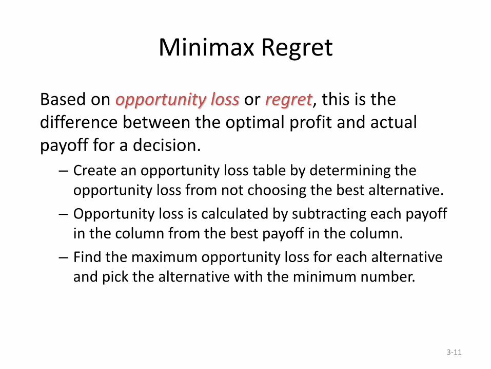
Minimax Regret
Based on opportunity loss or regret, this is the difference between the optimal profit and actual payoff for a decision.
– Create an opportunity loss table by determining the opportunity loss from not choosing the best alternative.
– Opportunity loss is calculated by subtracting each payoff in the column from the best payoff in the column.
– Find the maximum opportunity loss for each alternative and pick the alternative with the minimum number.

3-12
Minimax Regret
STATE OF NATURE
FAVORABLE MARKET ($) UNFAVORABLE MARKET ($)
200,000 – 200,000 0 – (–180,000)
200,000 – 100,000 0 – (–20,000)
200,000 – 0 0 – 0
Table 3.6
Determining Opportunity Losses for Thompson Lumber

3-13
Minimax Regret
Table 3.7
STATE OF NATURE
ALTERNATIVE FAVORABLE MARKET ($)
UNFAVORABLE MARKET ($)
Construct a large plant 0 180,000
Construct a small plant 100,000 20,000
Do nothing 200,000 0
Opportunity Loss Table for Thompson Lumber

3-14
Minimax Regret
Table 3.8
STATE OF NATURE
ALTERNATIVE FAVORABLE MARKET ($)
UNFAVORABLE MARKET ($)
MAXIMUM IN A ROW ($)
Construct a large plant
0 180,000 180,000
Construct a small plant
100,000 20,000 100,000
Do nothing 200,000 0 200,000 Minimax
Thompson’s Minimax Decision Using Opportunity Loss
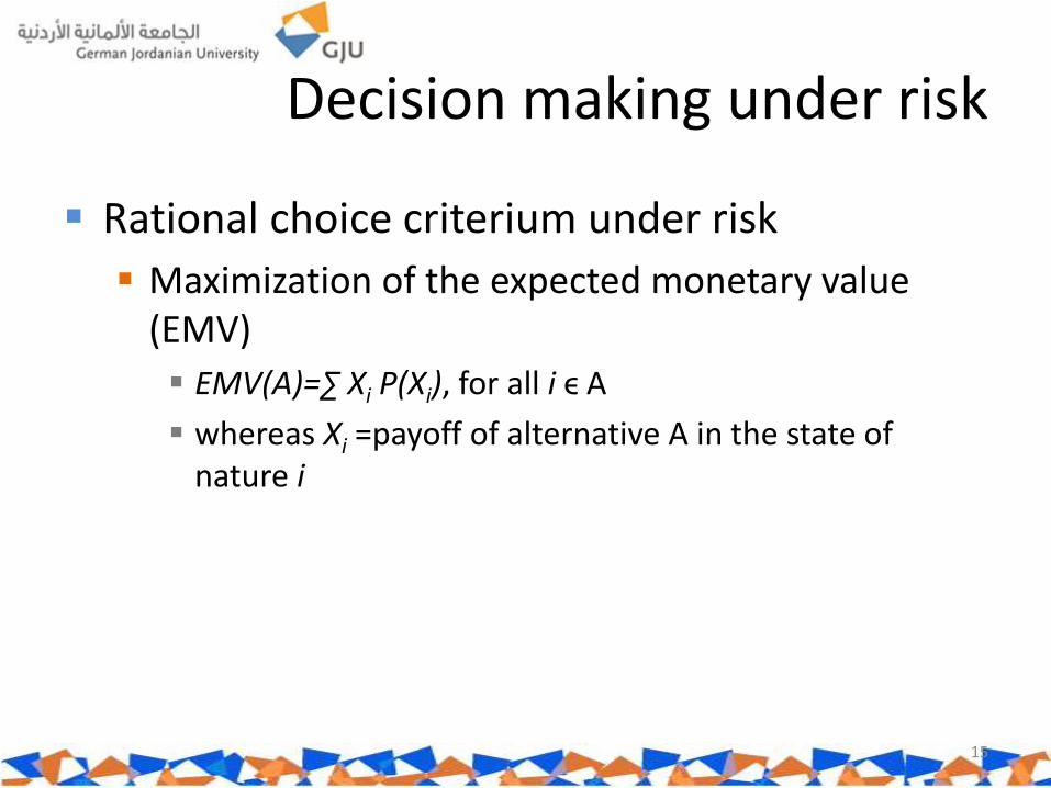
Decision making under risk
Rational choice criterium under risk
Maximization of the expected monetary value (EMV)
EMV(A)=∑ Xi P(Xi), for all i ϵ A
whereas Xi =payoff of alternative A in the state of nature i
15

Decision making under risk
Problem 3-20
a. What decision would maximize expected profits, if investment is the same?
16
alternative good bad
stock market 80000 -20000
bonds 30000 20000
CDs 23000 23000
probability 0,5 0,5
state of nature
EMV
30000
25000
23000

3-17
Expected Opportunity Loss
Expected opportunity loss (EOL) is the cost of not picking the best solution.
First construct an opportunity loss table.
For each alternative, multiply the opportunity loss by the probability of that loss for each possible outcome and add these together.
Minimum EOL will always result in the same decision as maximum EMV.
Minimum EOL will always equal EVPI.

3-18
Expected Opportunity Loss
EOL (large plant) = (0.50)($0) + (0.50)($180,000)
= $90,000
EOL (small plant) = (0.50)($100,000) + (0.50)($20,000)
= $60,000
EOL (do nothing) = (0.50)($200,000) + (0.50)($0)
= $100,000
Table 3.11
STATE OF NATURE
ALTERNATIVE FAVORABLE MARKET ($)
UNFAVORABLE MARKET ($) EOL
Construct a large plant 0 180,000 90,000
Construct a small plant
100,000 20,000 60,000
Do nothing 200,000 0 100,000
Probabilities 0.50 0.50
Minimum EOL

3-19
Sensitivity Analysis
Sensitivity analysis examines how the decision
might change with different input data.
For the Thompson Lumber example:
P = probability of a favorable market
(1 – P) = probability of an unfavorable market

3-20
Sensitivity Analysis
EMV(Large Plant) = $200,000P – $180,000)(1 – P)
= $200,000P – $180,000 + $180,000P
= $380,000P – $180,000
EMV(Small Plant) = $100,000P – $20,000)(1 – P)
= $100,000P – $20,000 + $20,000P
= $120,000P – $20,000
EMV(Do Nothing) = $0P + 0(1 – P)
= $0
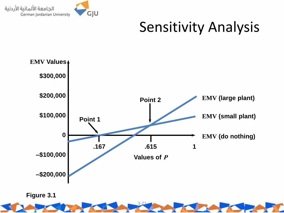
3-21
Sensitivity Analysis
$300,000
$200,000
$100,000
0
–$100,000
–$200,000
EMV Values
EMV (large plant)
EMV (small plant)
EMV (do nothing)
Point 1
Point 2
.167 .615 1
Values of P
Figure 3.1

3-22
Sensitivity Analysis
Point 1:
EMV(do nothing) = EMV(small plant)
000200001200 ,$,$ P 1670000120
00020.
,
,P
00018000038000020000120 ,$,$,$,$ PP
6150000260
000160.
,
,P
Point 2:
EMV(small plant) = EMV(large plant)

3-23
Sensitivity Analysis
$300,000
$200,000
$100,000
0
–$100,000
–$200,000
EMV Values
EMV (large plant)
EMV (small plant)
EMV (do nothing)
Point 1
Point 2
.167 .615 1
Values of P
BEST ALTERNATIVE
RANGE OF P VALUES
Do nothing Less than 0.167
Construct a small plant 0.167 – 0.615
Construct a large plant Greater than 0.615
Figure 3.1

Decision trees
Graphical way of representing (sequential) decision problem
Consisting in decision nodes and state of nature nodes
24
Decision node
State of nature nodes

Decision tree The decision tree for the „constructing a
plant“ problem would be
25
Favorable Market
Unfavorable Market
Favorable Market
Unfavorable Market
1
Construct
Small Plant 2
A Decision Node
A State-of-Nature Node

3-26
Thompson’s Decision Tree
Favorable Market
Unfavorable Market
Favorable Market
Unfavorable Market
1
Construct
Small Plant 2
Alternative with best EMV is selected
Figure 3.3
EMV for Node 1 = $10,000
= (0.5)($200,000) + (0.5)(–$180,000)
EMV for Node 2 = $40,000
= (0.5)($100,000) + (0.5)(–$20,000)
Payoffs
$200,000
–$180,000
$100,000
–$20,000
$0
(0.5)
(0.5)
(0.5)
(0.5)
3-27
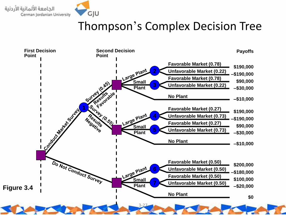
Thompson’s Complex Decision Tree
First Decision Point
Second Decision Point
Favorable Market (0.78)
Unfavorable Market (0.22)
Favorable Market (0.78)
Unfavorable Market (0.22)
Favorable Market (0.27)
Unfavorable Market (0.73)
Favorable Market (0.27)
Unfavorable Market (0.73)
Favorable Market (0.50)
Unfavorable Market (0.50)
Favorable Market (0.50)
Unfavorable Market (0.50) Small
Plant
No Plant
6
7
Small
Plant
No Plant
2
3
Small
Plant
No Plant
4
5
1
Payoffs
–$190,000
$190,000
$90,000
–$30,000
–$10,000
–$180,000
$200,000
$100,000
–$20,000
$0
–$190,000
$190,000
$90,000
–$30,000
–$10,000
Figure 3.4
3-28
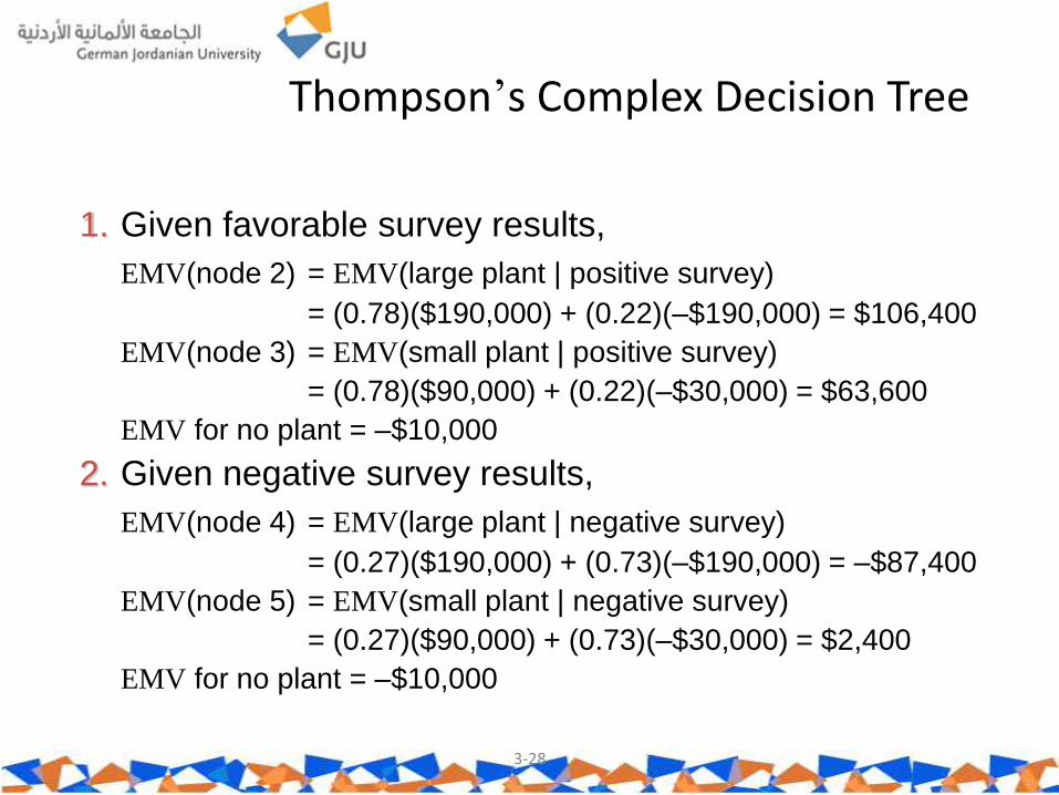
Thompson’s Complex Decision Tree
1. Given favorable survey results,
EMV(node 2) = EMV(large plant | positive survey)
= (0.78)($190,000) + (0.22)(–$190,000) = $106,400
EMV(node 3) = EMV(small plant | positive survey)
= (0.78)($90,000) + (0.22)(–$30,000) = $63,600
EMV for no plant = –$10,000
2. Given negative survey results,
EMV(node 4) = EMV(large plant | negative survey)
= (0.27)($190,000) + (0.73)(–$190,000) = –$87,400
EMV(node 5) = EMV(small plant | negative survey)
= (0.27)($90,000) + (0.73)(–$30,000) = $2,400
EMV for no plant = –$10,000
3-29
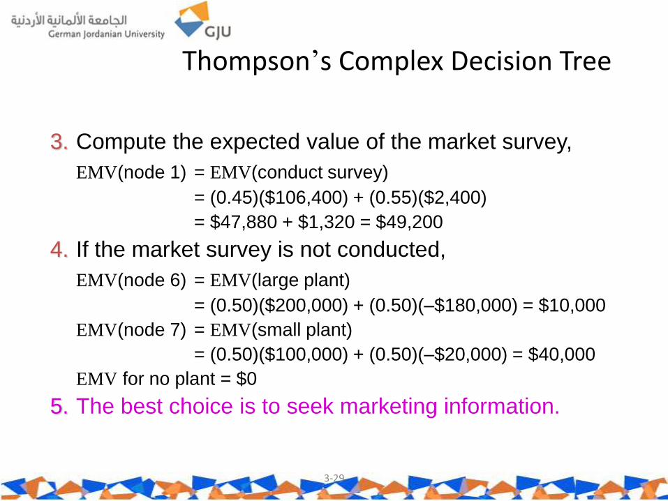
Thompson’s Complex Decision Tree
3. Compute the expected value of the market survey,
EMV(node 1) = EMV(conduct survey)
= (0.45)($106,400) + (0.55)($2,400)
= $47,880 + $1,320 = $49,200
4. If the market survey is not conducted,
EMV(node 6) = EMV(large plant)
= (0.50)($200,000) + (0.50)(–$180,000) = $10,000
EMV(node 7) = EMV(small plant)
= (0.50)($100,000) + (0.50)(–$20,000) = $40,000
EMV for no plant = $0
5. The best choice is to seek marketing information.
3-30
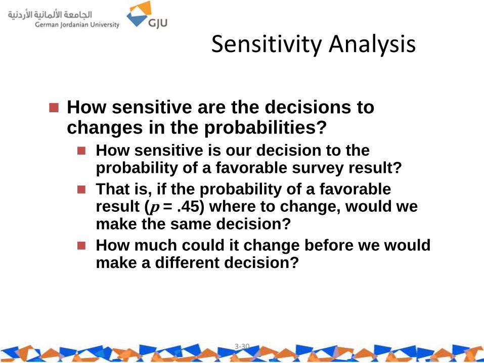
Sensitivity Analysis
How sensitive are the decisions to changes in the probabilities? How sensitive is our decision to the
probability of a favorable survey result?
That is, if the probability of a favorable result (p = .45) where to change, would we make the same decision?
How much could it change before we would make a different decision?

3-31
Sensitivity Analysis
p = probability of a favorable survey result
(1 – p) = probability of a negative survey result
EMV(node 1) = ($106,400)p +($2,400)(1 – p)
= $104,000p + $2,400
We are indifferent when the EMV of node 1 is the same as the EMV of not conducting the survey, $40,000
$104,000p + $2,400 = $40,000
$104,000p = $37,600
p = $37,600/$104,000 = 0.36
If p<0.36, do not conduct the survey. If p>0.36,
conduct the survey.

Bayesian probability update
Exercise
There are two urns containing colored balls. The first urn contains 50 red balls and 50 blue balls. The second urn contains 30 red balls and 70 blue balls. One of the two urns is randomly chosen (both urns have probability 0.50 of being chosen) and then a ball is drawn at random from one of the two urns. If a red ball is drawn, what is the probability that it comes from the first urn?
32

Case study
An oil exploration company considers three alternative investments, costing $100,000 each:
Bank investment: granting 10% after 5 years
Exploration A: either $200,000 or $-50,000 with a success probability of 0.50
Exploration B: either $300,000 or $-20,000 with a success probability of 0.60
What should the company do?
33

Case study
Considering only the explorations, how do the results change, if probabilities change?
It is further known, that the success probability of investment A is three times higher that that of B
How do the results change if the bank investment is considered, too?
34

3-35
Utility Theory
Monetary value is not always a true indicator of the overall value of the result of a decision.
The overall value of a decision is called utility.
Economists assume that rational people make decisions to maximize their utility.

3-36
Heads (0.5)
Tails (0.5)
$5,000,000
$0
Utility Theory
Accept Offer
Reject Offer
$2,000,000
EMV = $2,500,000 Figure 3.6
Your Decision Tree for the Lottery Ticket

3-37
Utility Theory
Utility assessment assigns the worst outcome a utility of 0, and the best outcome, a utility of 1.
A standard gamble is used to determine utility values.
When you are indifferent, your utility values are equal.
Expected utility of alternative 2 = Expected utility of alternative 1
Utility of other outcome = (p)(utility of best outcome, which is 1)
+ (1 – p)(utility of the worst outcome,
which is 0)
Utility of other outcome = (p)(1) + (1 – p)(0) = p

3-38
Standard Gamble for Utility Assessment
Best Outcome Utility = 1
Worst Outcome Utility = 0
Other Outcome Utility = ?
(p)
(1 – p)
Figure 3.7

3-39
Investment Example
Jane Dickson wants to construct a utility curve revealing her preference for money between $0 and $10,000.
A utility curve plots the utility value versus the monetary value.
An investment in a bank will result in $5,000.
An investment in real estate will result in $0 or $10,000.
Unless there is an 80% chance of getting $10,000 from the real estate deal, Jane would prefer to have her money in the bank.
So if p = 0.80, Jane is indifferent between the bank or the real estate investment.
3-40
Investment Example
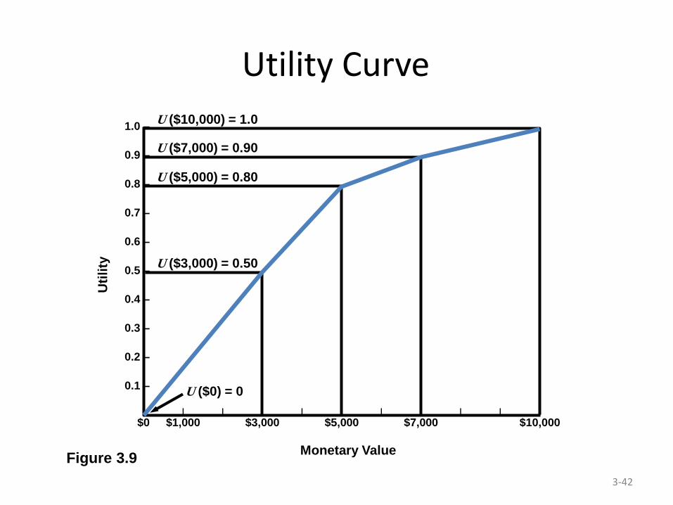
Figure 3.8
p = 0.80
(1 – p) = 0.20
$10,000 U($10,000) = 1.0
$0 U($0.00) = 0.0
$5,000 U($5,000) = p = 0.80
Utility for $5,000 = U($5,000) = pU($10,000) + (1 – p)U($0)
= (0.8)(1) + (0.2)(0) = 0.8

3-41
Investment Example
Utility for $7,000 = 0.90
Utility for $3,000 = 0.50
We can assess other utility values in the same way.
For Jane these are:
Using the three utilities for different dollar amounts, she can construct a utility curve.
3-42
Utility Curve
U ($7,000) = 0.90
U ($5,000) = 0.80
U ($3,000) = 0.50
U ($0) = 0
Figure 3.9
1.0 –
0.9 –
0.8 –
0.7 –
0.6 –
0.5 –
0.4 –
0.3 –
0.2 –
0.1 –
| | | | | | | | | | |
$0 $1,000 $3,000 $5,000 $7,000 $10,000
Monetary Value
Uti
lity
U ($10,000) = 1.0

3-43
Utility Curve
Jane’s utility curve is typical of a risk avoider. She gets less utility from greater risk.
She avoids situations where high losses might occur.
As monetary value increases, her utility curve increases at a slower rate.
A risk seeker gets more utility from greater risk As monetary value increases, the utility curve increases
at a faster rate.
Someone with risk indifference will have a linear utility curve.

3-44
Preferences for Risk
Figure 3.10
Monetary Outcome
Uti
lity
Risk Avoider
Risk Seeker
3-45
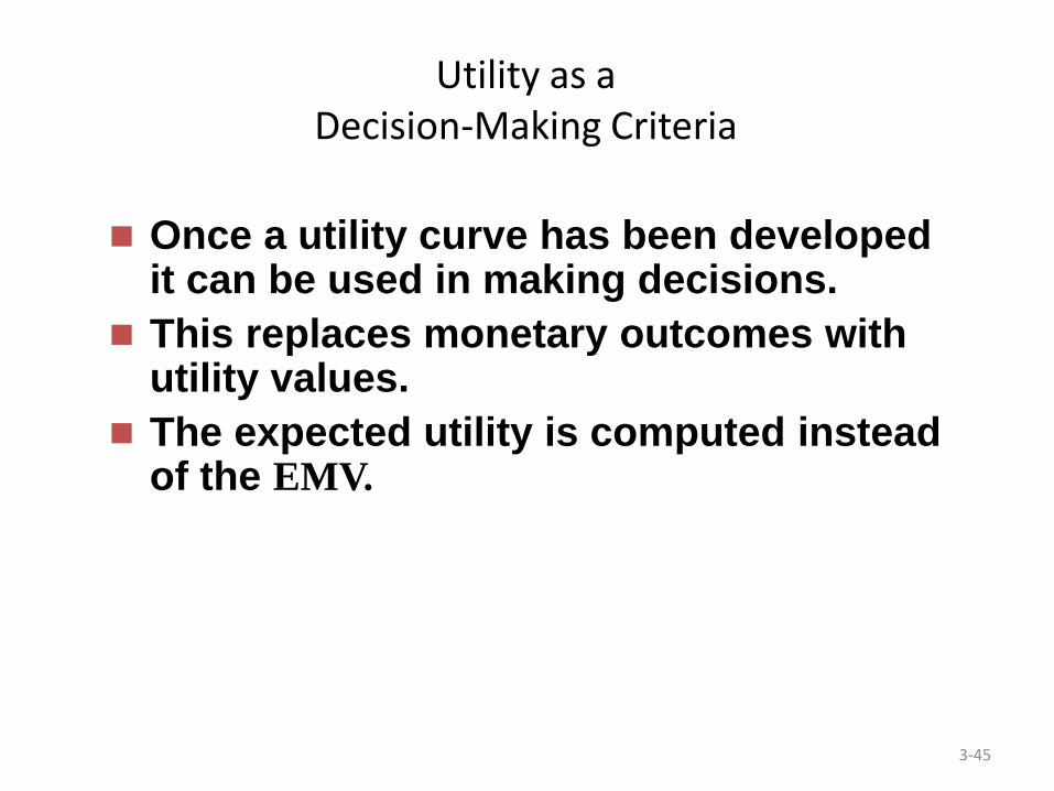
Utility as a Decision-Making Criteria
Once a utility curve has been developed it can be used in making decisions.
This replaces monetary outcomes with utility values.
The expected utility is computed instead of the EMV.

3-46
Utility as a Decision-Making Criteria
Mark Simkin loves to gamble.
He plays a game tossing thumbtacks in the air.
If the thumbtack lands point up, Mark wins $10,000.
If the thumbtack lands point down, Mark loses $10,000.
Mark believes that there is a 45% chance the thumbtack will land point up.
Should Mark play the game (alternative 1)?

3-47
Utility as a Decision-Making Criteria
Figure 3.11
Tack Lands Point Up (0.45)
$10,000
–$10,000
$0
Tack Lands Point Down (0.55)
Mark Does Not Play the Game
Decision Facing Mark Simkin
3-48
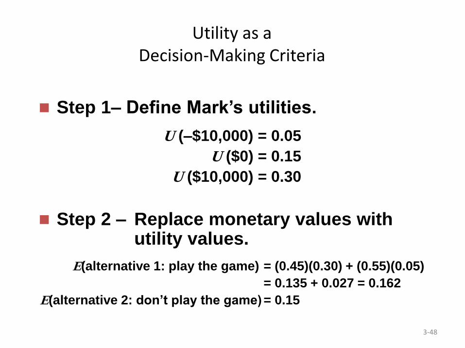
Utility as a Decision-Making Criteria
Step 1– Define Mark’s utilities.
U (–$10,000) = 0.05
U ($0) = 0.15
U ($10,000) = 0.30
Step 2 – Replace monetary values with utility values.
E(alternative 1: play the game) = (0.45)(0.30) + (0.55)(0.05)
= 0.135 + 0.027 = 0.162
E(alternative 2: don’t play the game) = 0.15

3-49
Utility Curve for Mark Simkin
Figure 3.12
1.00 –
0.75 –
0.50 –
0.30 –
0.25 –
0.15 –
0.05 –
0 – | | | | |
–$20,000 –$10,000 $0 $10,000 $20,000
Monetary Outcome
Uti
lity

3-50
Utility as a Decision-Making Criteria
Figure 3.13
Tack Lands Point Up (0.45)
0.30
0.05
0.15
Tack Lands Point Down (0.55)
Don’t Play
Utility E = 0.162
Using Expected Utilities in Decision Making