quantitative assessment of agricultural runoff and soil

Quantitative Assessment of Agricultural Runoff andSoil Erosion Using Mathematical Modeling:Applications in the Mediterranean RegionG. ARHONDITSIS*,1

Department of Marine SciencesUniversity of the Aegean81100 Mytilene, Greece

C. GIOURGAA. LOUMOUM. KOULOURIDepartment of Environmental StudiesUniversity of the Aegean81100 Mytilene, Greece

ABSTRACT / Three mathematical models, the runoff curvenumber equation, the universal soil loss equation, and themass response functions, were evaluated for predicting non-point source nutrient loading from agricultural watersheds ofthe Mediterranean region. These methodologies were appliedto a catchment, the gulf of Gera Basin, that is a typical terres-trial ecosystem of the islands of the Aegean archipelago. Thecalibration of the model parameters was based on data from

experimental plots from which edge-of-field losses of sedi-ment, water runoff, and nutrients were measured. Special em-phasis was given to the transport of dissolved and solid-phasenutrients from their sources in the farmers’ fields to the outletof the watershed in order to estimate respective attenuationrates. It was found that nonpoint nutrient loading due to sur-face losses was high during winter, the contribution being be-tween 50% and 80% of the total annual nutrient losses fromthe terrestrial ecosystem. The good fit between simulated andexperimental data supports the view that these modeling pro-cedures should be considered as reliable and effective meth-odological tools in Mediterranean areas for evaluating potentialcontrol measures, such as management practices for soil andwater conservation and changes in land uses, aimed at dimin-ishing soil loss and nutrient delivery to surface waters. Further-more, the modifications of the general mathematical formula-tions and the experimental values of the model parametersprovided by the study can be used in further application ofthese methodologies in watersheds with similar characteris-tics.

One of the problems frequently involved in coastalmanagement is that of distinguishing between pointand nonpoint discharges, which is essential for effectiveprotection of seawater quality (Paerl 1997). Pointsources enter the pollution transport routes at discrete,identifiable locations and usually can be measured di-rectly. On the other hand, nonpoint sources enter sur-face waters in a diffuse manner and at intermittentintervals that are related mostly to the occurrence ofmeteorological events. They cannot be monitored attheir point of origin and their exact source is difficultor impossible to trace. Therefore, nonpoint sources areinherently difficult to measure and they cannot be

assessed in terms of effluent limitations (Novotny andChesters 1981, Marchetti and Verna 1992).

The difficulties and inaccuracies concerning theprediction of soil loss and direct runoff from varioussoil and crop combinations encountered in watershedsand the retention and transport processes of nutrientsthrough these systems were partially surpassed by theuse of mathematical models (Deaton and Winebrake1999). Individual components of basins have beenmodeled with varying levels of success to attempt tounderstand the interdisciplinary nature of processesoperating at the watershed level (Borah 1989, Huberand others 2000). These models can be classified ac-cording to their level of sophistication and potentialfield of application, and each class is efficient for arange of simulations, which, in principle, cover anylevel of detail the user might deem necessary (Bouraouiand Dillaha 1996).

During the last decade, comprehensive-modelingconstructions, focused on deterministic, stochastic, lin-ear or nonlinear interpretations of the coastal systems’behavior have reached an advanced level in NorthAmerica and Europe (Nikolaidis and others 1998, Bas-

KEY WORDS: Nonpoint source pollution; Mediterranean region; Coastalmanagement; Mathematical model; Agricultural runoff;Soil erosion

1Present address: Department of Civil and Environmental Engineer-ing, University of Washington, 313B More Hall, Box 352700, Seattle,Washington, USA

*Author to whom correspondence should be addressed; email:[email protected]

DOI: 10.1007/s00267-001-2692-1

Environmental Management Vol. 30, No. 3, pp. 434–453 © 2002 Springer-Verlag New York Inc.

nyat and others 1999, Ekholm and others 1999). Mean-while, similar approaches in the Mediterranean regionare still in an early phase and considerable gaps in theliterature exist with regard to the computation of re-gionalized relationships and the objective calibration ofthe various parameters of well-known algorithms (Bag-arello and D’Asaro 1994). Existing knowledge in thisgeographic area is primarily based on strict applicationsof international mathematical developments, withoutany adjustment for the unique structure of the Medi-terranean-type ecosystems and the implications of thelocal physicochemical and biological factors.

The goal of this work was to develop a consistentmethodology for assessing nonpoint source pollutionin the Mediterranean region. The effectiveness and thepredictability of three models, the runoff curve numberequation (CNE), the universal soil loss equation(USLE), and the mass response functions (MRF), weretested in a typical terrestrial ecosystem of the Mediter-ranean region. The study also provides the fundamen-tal framework so that the requirements of the particularmathematical models are met, whereas conceptualmodifications in the basic analysis of soil erosion andsurface runoff are proposed with a view of improvingthe quantification of the nutrient outflows of the eco-systems. Finally, a critical discussion tends to emphasizethe defects of these methods and the need for detailedsensitivity analysis and validation of these models under

various meteorological conditions, agricultural prac-tices, and landscape characteristics of the Mediterra-nean area.

Methodology

The Study Area

This study was conducted within the gulf of GeraBasin, a 194-km2 drainage area on the island of Lesvos(Figure 1). The flora on this island belongs to the OleoCeratonion zone. According to Thornthwaite’s classifica-tion system, the local climate is of the type C1dB3� b�4,characterized by an annual rainfall between 600 and800 mm; an annual evapotranspiration potential of 900mm, and a high mean air temperature of 19°C (Arhon-ditsis and others 2000b). The area is considered as atypical terrestrial ecosystem of the Mediterranean re-gion that is characterized mostly by shallow and infer-tile soils, steep slopes, water deficiency, and limitedarable lands. The geological substrate consists mostly ofmetamorphic rocks (marbles, mica schists), igneousrocks (granites, basalts), and alluvial depositions. Mostof the local rivers have a torrential regime that is con-siderably influenced by local precipitation characteris-tics and physiographic features of the area. Figure 2illustrates the potential hydrographic characteristics ofthe watershed and shows that most of these flow paths

Figure 1. Gulf of Gera, Island of Lesvos, Greece showing the sampling sites of the marine (GG1-GG8) and terrestrial ecosystems.Numbers 1, 2, 3, and 4 correspond to the land cover categories: cultivated olive groves, abandoned olive groves, maquis, andwetlands, respectively. Letters A, B, and C correspond to altitudes of �150, 150–300, and �300 m, respectively.

Modeling Nonpoint Pollution in the Mediterranean Region 435

usually remain inactivated but can occasionally contrib-ute to the routing of the runoff volumes of stormevents, especially during the years of high annual rain-fall. Shortage of arable land in the watershed has beencompensated by the construction of extensive systemsof terraces that minimize soil erosion.

Table 1 lists the most abundant vegetation types ofthe area, as result of a landscape analysis based onthe unsupervised and supervised classification of

Landsat Thematic Mapper (TM) images (Hatzopou-los and others 1992). The landscape is characterizedby a traditional monoculture of olive trees (Olea eu-ropea) occupying 60% of the total area of the water-shed. Two types of olive plantations can be distin-guished; cultivated and abandoned. Cultivatedplantations are the olive groves in which cultivationtakes place annually and wild woody plants are lim-ited. Abandoned plantations are olive groves in

Figure 2. The hydrographic characteristics of Gulf of Gera’s watershed.

436 G. Arhonditsis and others

which the canopy of the olive trees is limited, wildwoody plants exist, and natural vegetation of olivetrees has begun. The mountainous zones of thecatchment (�32%) are covered with evergreensclerophyllous plant communities (maquis),phrygana in combination with coniferous trees (Pi-nus brutia), constituting the climax stage of naturalecosystems in the Mediterranean region. Further-more, the landscape of the northwestern part of thewatershed is characterized by the presence of wet-lands (3.5%) used as pastures for sheep and goatsyear round. The structure and the dynamic behaviorof these characteristic plant types of the Mediterra-nean region were studied by a dense sampling net-work (Figure 1), whereas the experimental proce-dure and further details about the results arereported elsewhere (Arhonditsis and others 2000b).

The subsequent seawater body, the gulf of Gera, isa semienclosed marine ecosystem with a mean depthof 10 m and a total volume of 9 � 108 m3. It isinfluenced by significant nutrient fluxes from agri-cultural runoff and soil erosion, especially during thewinter period when the contribution is between 40%and 60% of the total nutrient flux (Arhonditsis andothers 2000a). The chemical and biological informa-tion collected from eight sampling sites (Figure 1),revealed that the mean concentrations of nitrate,

phosphate, organic nitrogen, and chlorophyll arerather high, being 0.55, 0.19, 7.93 �g-at/liter and0.98 �g/liter, respectively. These mean values arecharacteristic of a mesotrophic marine environmentwith eutrophic trends (Kitsiou and Karydis 1998).Thus, the potential threat for a further decline in thequality of the marine ecosystem indicates a need forthe development of management schemes that con-trol nonpoint pollution.

Application of Nonpoint Pollution Models

Inventory of source areas. Three nonpoint source pol-lution models were applied to the watershed to inven-tory its physicochemical and biological properties. Thisprocedure was simplified considerably by the divisionof the heterogeneous and complex system into compu-tational elements or grid cells. Cell size selection wasinvestigated through sensitivity analysis of the models’input parameters (Vieux and Needham 1993), whichindicated that in all cases the best fit with the experi-mental results was obtained using a grid of 0.25 � 0.25km. The discrimination of the cell characteristics (i.e.,soil type, land use, management or treatment practice,slope length, and distance from the nearest stream) wassupported by the use of GIS (Hatzopoulos and others1992). Nutrient variability, determined from the previ-ous mentioned study, focused on the temporal patterns

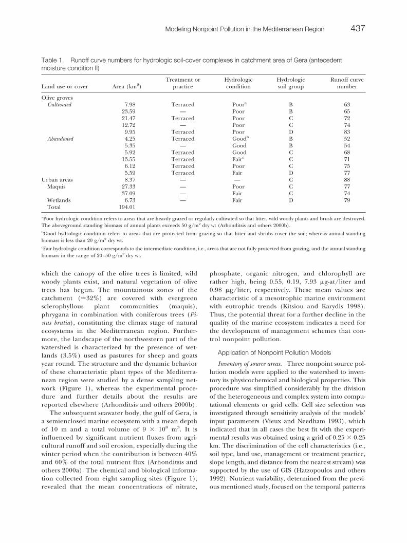
Table 1. Runoff curve numbers for hydrologic soil-cover complexes in catchment area of Gera (antecedentmoisture condition II)

Land use or cover Area (km2)Treatment or

practiceHydrologiccondition

Hydrologicsoil group

Runoff curvenumber

Olive grovesCultivated 7.98 Terraced Poora B 63

23.59 — Poor B 6521.47 Terraced Poor C 7212.72 — Poor C 749.95 Terraced Poor D 83

Abandoned 4.25 Terraced Goodb B 525.35 — Good B 545.92 Terraced Good C 68

13.55 Terraced Fairc C 716.12 Terraced Poor C 755.59 Terraced Fair D 77

Urban areas 8.37 — — C 88Maquis 27.33 — Poor C 77

37.09 — Fair C 74Wetlands 6.73 — Fair D 79Total 194.01

aPoor hydrologic condition refers to areas that are heavily grazed or regularly cultivated so that litter, wild woody plants and brush are destroyed.The aboveground standing biomass of annual plants exceeds 50 g/m2 dry wt (Arhonditsis and others 2000b).bGood hydrologic condition refers to areas that are protected from grazing so that litter and shrubs cover the soil; whereas annual standingbiomass is less than 20 g/m2 dry wt.cFair hydrologic condition corresponds to the intermediate condition, i.e., areas that are not fully protected from grazing, and the annual standingbiomass in the range of 20–50 g/m2 dry wt.


of inorganic nutrients and organic nitrogen over themost abundant vegetation types of the area (Arhondit-sis and others 2000b). Figure 3 represents the spatialdistribution of soil concentrations of nitrate, ammo-nium, and phosphate over the gulf of Gera basinduring the winter period when the most significantrainfall events take place. The values of nutrientsassigned to the intermediate cells that did not coin-cide with experimental sites (Figure 1), were ob-tained by interpolation using the inverse distance-

weighting method (Watson and Philip 1985). Theestimation of the solid and dissolved phase fractionwas obtained through Langmuir (for phosphates)and Freundlich (for ammonium) isotherms, whereasthe nitrate was assumed to be totally dissolved (No-votny and others 1978, Novotny and Chesters 1981).Daily and hourly precipitation records, used for thedetermination of the various model parameters, wereavailable from a meteorological station locatedwithin the watershed.

Figure 3. Spatial distribution of total soil concentrations(�g/cm3) of (a) nitrate, (b) ammonium, and (c) phosphateover the gulf of Gera Basin during the winter period.


Runoff curve number equation

Fundamental concepts. This method is a convenientmeans of estimating excess rain, and the general for-mulas describing the rainfall-runoff events are:

Qkt ��Rkt � 0.2 � Skt�

2

2.54 � �Rkt � 0.8 � Skt�(1)

CNkt �1000

10 �Skt

2.54

(2)

in which Rkt is the rainfall (centimeters), on day t fromsource area k, Skt is a detention parameter (centime-ters), Qkt is the runoff (centimeters), and CNkt is anexpression called “curve number,” which is a tabulatedfunction of soil hydrologic group, land cover, manage-ment, hydrologic condition, and antecedent soil mois-ture (Haith and Tubbs 1981). The term “soil hydro-logic group” refers to the classification of the watershedsoils into four hydrologic groups, according to theirpermeability and runoff potential (Chow and others1988): group A contains soils with sands or gravel,exhibiting low surface runoff potential; groups B (mod-erately coarse texture) and C (moderately fine texture)present intermediate to slow rates of water transmis-sion, respectively; and group D soils have high surfacerunoff potential, consisting chiefly of clay soils with ahigh swelling potential, soils with a permanently highwater table, or shallow soils over nearly imperviousmaterial (Novotny and Chesters 1981).

The nutrient losses from a unit source area k, due toa runoff event on day t, are given by (Haith and Tubbs1981):

LD � 10 � Cdkt � Qkt � TDk (3)

where LDkt is the dissolved-phase fraction of nutrientloss in kilograms per square kilometer, Cdkt is the nu-trient concentration in dissolved phase measured inmilligrams per liter TDk is a transport factor indicatingthe fraction of dissolved-phase nutrient that movesfrom the edge of the source area to the watershedoutlet, and Qkt is the rainfall height in centimeters. Thetotal dissolved nutrient export (LD) for a specific timeperiod is calculated in equation 4, by multiplying thelosses from each source by its respective area (Ak, inkilometer2) and summing over all unit source areas anddays in the time period:

LD � 10 � �t

�k

Cdkt � Qkt � TDk � Ak (4)

Thus, the implementation of this method requires es-timates of runoff, pollutant concentrations, and atten-

uation during the transport from each unit source areawithin the watershed.

Illustrative applications. One of the most importantaspects of the model application was the determinationof the runoff curve number values that correspond tothe characteristic soil/cover complexes of the area(Hauser and Jones 1991). In the present work, thederived runoff curves were based on experimental re-sults, extracted from the field plots of the sites in Figure1. This network covered the entire extent of the water-shed and took into consideration all the possible com-binations of soil hydrologic groups, land uses or covers,and management and hydrologic conditions encoun-tered in the study system. The size of the experimentalplots was variable (10–26 m2) and at least three repe-titions per combination were used as a minimum stan-dard of objectivity (Arhonditsis and others 2000b). Ta-ble 1 shows the results for the average soil moisturelevel of the area, the so-called antecedent moisturecondition II (Novotny and Chesters 1981). Moreover,the effects of the antecedent soil moisture on the run-off curve values were obtained by the use of equation 5(Hawkins 1978):

CN2 �1200

1200CN1

[ET (R Q)]

2.54

(5)

where CN1 and CN2 are the runoff curve values at times1 and 2, respectively, R and Q are the interim rainfallinputs (centimeters) and runoff losses (centimeters),and ET is the sum of evapotranspiration and drainagelosses (centimeters) during this time interval and werebased on actual field measurements (Arhonditsis1998). The minimal and maximal values of the runoffcurves reflecting the lowest and the highest runoff po-tential of each unit source area, the so-called anteced-ent moisture conditions I and III, were based on theequations 6 and 7 (Chow and others 1988):

CNI �CNII

2.334 � 0.01334 � CNII(6)

CNIII �CNII

0.4036 � 0.0059 � CNII(7)

where CNI, CNII, and CNIII are the runoff curve valuesof the three soil moisture classes.

The most fundamental factor affecting the concen-trations of dissolved nutrients in runoff is the quantityof available nutrients in the soil. Although these nutri-ents may come from various sources, the total availablenitrogen and phosphorus for a specific land cover isrelatively constant and thus dissolved nutrient concen-


trations in runoff are primarily functions of the vegeta-tion types in the source areas (Scholefield and Stone1995, Summers and others 1999). Table 2 shows flow-weighted average dissolved ammonium, nitrate, andphosphate concentrations in runoff from the mostabundant plant types of the watershed, measured onthe field plots over three years of natural precipitation.Since average nutrient concentrations often differ sig-nificantly over the year, the concentrations were sepa-rated into cold- and warm-weather categories in orderto increase model accuracy. Given the climatic condi-tions of the Mediterranean region, cold-weather condi-tions were assumed to last from the first day in whichthe 30-day running average temperature fell below10°C (early December) until the first day in which the30-day average exceeded 10°C (the end of February orearly March). The warm-weather concentrations arehigher as a result of fertilizer applications and micro-bial activity, accelerated by the favorable abiotic factors(temperature, solar radiation, moisture) that prevailduring this time period (Moreno and Oechel 1995).

Numerous applications of the CNE are based on theassumption that both runoff and dissolved pollutantsare conserved during their movement from the farm-er’s fields to the watershed outlet. This perception isvalid for dissolved substances (i.e., nitrates) that areattenuated primarily by biological phenomena andthus are not likely to be significantly reduced (Haithand Tubbs 1981). Consequently, a transport factorequal to 1 was considered for dissolved losses of nitratefor all the unit source areas of the watershed. On theother hand, there may be opportunities for dissolvedchemicals such as phosphate and ammonium to beremoved from the runoff solution by adsorption or bychemical reactions with the topsoil. In these cases, theassumption that TDk � 1 would be invalid, especially forsingle isolated events, leading to overestimation of theexport of dissolved pollutants from watersheds. Thus, a

new transport factor for phosphate and ammonium wasapplied, given by equation 8:

TDk � e � � � dk (8)

where dk is the downslope distance (meters) from thecenter of source area k to the nearest identifiable drain-age channel, and � is a coefficient, which was found,after model calibration, to be 0.001 for ammonium and0.002 for phosphate.

Mass response functions

Fundamental concepts. The mass response functionsare defined as probability–density functions associatedwith the random holding time of the water particleswithin the basin and conditional on the time of occur-rence of the storm event. The particle-holding timesare assumed to drive mass transfer through contactbetween phases and control the chemical process ofsorption phenomena (Rinaldo and Marani 1987). Thefundamental model structure may be described as thecombination of a water quality component, based on asimple mass balance, with the Nash conceptual hydro-logic model of rainfall–runoff transformations (Ben-doricchio and Rinaldo 1986). The latter componentmodels the watershed as a cascade of continuouslystirred tank reactors. According to this concept, thetransfer function of a hydrologically active unit area torainfall events distributed in time according to i( ) isbuilt by convolution as:

Q�t;n;k� � �0

t

h�t � ;n;k� � i� �d (9)

where

h�t;n;k� �l

k � � �n�� t/k�n � 1 � e � t/k (10)

Table 2. Dissolved ammonium, nitrate and phosphate,a concentrations in runoff from most abundant watershedland-cover categories of watershed

Land cover

Concentrations (mg/liter)

Warm weather Cold weather

Ammonium Nitrate Phosphate Ammonium Nitrate Phosphate

Olive grovesCultivated 0.82 � 0.15 1.21 � 0.18 0.31 � 0.08 0.61 � 0.08 1.02 � 0.12 0.22 � 0.05Abandoned 0.53 � 0.09 0.72 � 0.10 0.22 � 0.07 0.30 � 0.06 0.61 � 0.05 0.20 � 0.04

Urban areas 0.81 � 0.18 0.81 � 0.11 0.32 � 0.10 0.81 � 0.09 0.84 � 0.08 0.34 � 0.05Maquis 0.21 � 0.08 0.34 � 0.08 0.12 � 0.02 0.23 � 0.03 0.19 � 0.04 0.15 � 0.02Wetlands 0.62 � 0.17 0.72 � 0.12 0.29 � 0.05 0.50 � 0.04 0.58 � 0.10 0.20 � 0.03

aRefers to all the filterable molybdate-reactive P.


where Q(t;n;k) is the flow output (cubic meters perhour) per unit source area (square meters), h(t;n;k) isthe ordinate of the instantaneous unit hydrograph(hours1), is the lag time that corresponds to the timeinterval between maximum rain excess and the peak ofthe runoff (hours), i( ) is the impulse hyetograph(meters per hour), n is a dimensionless watershed char-acteristic representing approximately the number ofreservoirs, (n) is the gamma function of n, and k is astorage constant (hours1) related to the time of travelof rainwater from the most remote point on the water-shed to the watershed outlet te (time of equilibrium ortime of concentration) by the expression k � te/n.

Furthermore, the conceptual scheme for the chem-ical mass transfer, in a continuously stirred tank reac-tor, is given by:

�c�t

� h�ce � c� (11)

where c is the current nutrient concentration (mili-grams per liter) in the runoff volume (mobile phase), ce

is the equilibrium concentrations (miligrams per liter)in the dissolved-phase (an interphase where solid orfixed and mobile phases are in equilibrium), and h is amass transfer coefficient (hours1) that measures theactual speed of chemical transfer from the interphaseto the bulk of the runoff (Zingales and others 1984). Inthe case that ce is a time-independent variable and h isa spatial and temporal constant, the flow rate q of anutrient and the total quantity Z in the watershed out-let, are given by the following unit-mass response func-tions:

q�t; n; k; h; c�e� � c�e � �Q�t; n; k�

� � kk � h�

n

� Q�t; n; k � h�� (12)

Z�t; n; k; h; c�e� ��0

t

q�t; n; k; h; c�e�dt � c�et � �V�t; n; k�

� � kk � h�

n

� V�t; n; k � h�� (13)

c�e � �y1

y2 �x1

x2

c�e� x, y�dxd y (14)

where q(t;n;k;h;c�e) is the nutrient flow rate (miligramsper hour), Z(t,n,k,h,c�e) is the total nutrient load (milli-grams) at time t, Q(t;n;k) is the flow output (m3 perhour) and V(t;n;k) is the runoff volume discharge (cu-bic meters) at time t per unit area (square meters).

Finally, the term c�e constitutes an innovation of thepresent study, referring to the spatial variability of c�eover the basin. It is computed by integrating the distri-bution function ce(x,y) of the dissolved-phase concen-trations over the catchment area, where x1, x2, y1, and y2

correspond to the coordinates of the watershed bound-aries.

Illustrative applications. One principal question ofthe model application is how many linear pools areneeded for the simulation of solute transport in thehydrologic response (Bendoricchio and Rinaldo 1986).In the present work, the optimum fitting between com-puted runoff and measured hydrographs was producedby applying n � 2. Furthermore, the estimation of thescale parameter k was sought from two alternative meth-ods in the literature; the parameterization of the instan-taneous unit hydrograph in terms of Horton orderratios or the application of Manning’s surface rough-ness factor-based equations to compute the time ofequilibrium (Novotny and Chesters 1981, Rosso 1984,Chow and others 1988). Given the ambiguous hydro-graphic status of the study watershed and the torrentialregime of the local rivers, the determination of someessential input requirements of the former approach,such as the geomorphologic characteristics of the basin(i.e., the Horton’s numbers RA, RB, and RL or the meanlength of ith order stream), is rather complicated andinaccurate. Thus, the latter method is deemed moreappropriate and reliable for areas characterized by thegeomorphoclimatic conditions of the Mediterraneanregion. The estimation of the time of equilibrium te foreach source area was computed by the following for-mulas:

te � te1 � te2 (15)

te1 � 6.9 �L1

0.6 � nM10.6

i0.4 � S10.3 (16)

te2 � 0.017 �L2 � nM2

R2/3 � S20.5 (17)

where te1 and te2 are the time lengths (minutes) of theoverland and channel flow, respectively, i the rain in-tensity (millimeters per hour), R is the hydraulic radius(meters) of the channel defined as cross-sectional areadivided by the wetted perimeter, S1 and S2 are the meanslopes (meters per meter) of the overland and channelflow, L1 and L2 are the lengths (meters) of the overlandand channel flow, nM1 and nM2 are the Mannings sur-face roughness factors, which vary with the groundcover. Table 3 presents literature-based values of theManning factors (Chow and others 1988), adjustedduring the calibration process in order to obtain better


fit between simulated and experimental data. Thesevalues can also be extrapolated and tested in othercatchments of the Mediterranean region characterizedby the same land uses or ground covers with similarqualitative characteristics and species composition. Thefirst equation of the overland flow was developed for atwo-plane V-shaped watershed using the kinematic waveapproximation, but can account for wider and morecomplex representations after the division of the water-shed into homogeneous computational elements(Chow and others 1988). On the other hand, the sec-ond equation presumes a uniform flow of runoff in theopen channels, a prerequisite that seems to be valid,since the depth of flow in the local torrents and rills isapproximately constant in the direction of flow (Albert-son and Simons 1964).

Another critical point of the model development wasthe incorporation of the term c�e that describes thespatial variability of the dissolved-phase concentrationsof nitrate, ammonium, and phosphate over the basin.This addition amplifies the role of the features of thestudy system in the modeling procedure, resulting inmore realistic results (Bendoricchio and Rinaldo 1986,Rinaldo and Marani 1987). The description of the equi-librium concentrations c�e as a function of space wasobtained in two ways: (1) the interpolation method,computing the spatial heterogeneity of dissolved-phase

nutrients, similar to the method already used for thetotal soil concentrations, and (2) multiple regressionanalysis (Draper and Smith 1981). In this particularcase, a preliminary test (not reported in this paper)showed that the later approach produced a better fitbetween observed and computed values, and it wastherefore considered more suitable for the explicit ex-pression of the mass response functions. The watershedwas divided into six subcatchments (outlined in Figure2), where separate sets of equations were formed inorder to increase accuracy of the method (Arhonditsis1998). Seasonality effects (i.e., variations of ce at timescales larger than that of the hydrologic response) werealso taken into account by defining three (four seasonsminus one) dummy variables (Golfinopoulos and oth-ers 1998). The seasons with the dummy variables werewinter (win), spring (spr) and autumn (aut). As anexample, the values of the variable (win) were deter-mined by the expression:

win � � 1 if the simulated runoff event takesplace in the winter period

0 otherwise

Preliminary data analysis involved the testing of normal-ity using the Kolmogorov-Smirnov test and data trans-formations in the cases of a poor fitting to the normaldistribution. The data were also tested for homoscedas-ticity using the Durbin-Watson test, whereas the rela-tionships between the variables were examined by sim-ple correlation (Vounatsou and Karydis 1991). Theequations describing the spatial distribution of the dis-solved-phase concentrations of nitrate, ammonium,and phosphate over the western part of the basin (sim-ilar equations were developed for the rest parts of thewatershed), are the following:

NO3(e) � 44.3868 � x 32.0318 � y

6.3751 � win � y 14.9041 � spr

11.1821 � x � y5.4032 � x2 (18)

NH4(e) � 0.3551 � x 0.7564 � y2 0.3790 � win � y

0.3113 � spr 0.3066 � x � y (19)

logPO4(e) � 0.2272 � x 0.1492 � y

0.0344 � win � �y 0.0209 � spr

0.3555 � x � y (20)

0.15 � x � 5.6 km and 0.01 � y � 1.5 km

where the ranges of the variables x and y are defined bythe coordinates of the remotest experimental sitesalong the two dimensions of the basin. Generally, themethod has resulted in statistically significant regres-

Table 3. Mean values of the Manning’s roughnessfactor, nM, for overland and channel flow over studywatersheda

Manning’sroughness

factor(nM)

a) Overland flowOlive groves

Cultivated, ground cover� 60% 0.2830–60% 0.22� 30% 0.16

Abandoned, ground cover�50% 0.38�50% 0.32

Maquis, ground cover�70% 0.1835–70% 0.12�35% 0.08

Channel flowEarth, straight and uniform 0.028

Earth and winding 0.042Few trees, stones, or brush 0.063

Weeds and stones 0.055aLiterature-based values of Manning factors (Chow and others 1988),adjusted during the calibration process.


sion models at the 5% level, with satisfactory multipledetermination coefficients (R2 � 0.75) for all subcatch-ments of the watershed (Arhonditsis 1998).

The calibration of the model was obtained by sys-tematic sampling and flow measurements on an hourlybasis during the occurrence of several rainfall–runoffevents. The samples were taken from the outlets of thetwo basic torrents of the area, located on the northernand western part of the watershed. Analytical work wasfocused on the determination of nitrate, ammonium,and phosphate concentrations in the bulks of runoff(Arhonditsis 1998). Finally, the lack of experimentalmeasurements of the base flow for some rainfall eventswas overcome by the hydrograph separation technique,based on drawing a straight line from the point of riseto a point on the lower portion of the recession seg-ment of the hydrograph (Chow 1964).

Universal Soil Loss Equation

Fundamental concepts. The universal soil loss equa-tion (USLE) is the most common estimator of soil losscaused by upland erosion and when applied to individ-ual rainstorms it is formulated as:

Xkt � Rt � Ck � Kk � Lk � Sk � Pk (21)

where Xkt is soil erosion (tons per hectare) on day tfrom source area k, Ck is the crop management factor(unitless), which reflects the effects of cropping andmanagement practices on erosion rates, Kk is the soilerodibility factor, (tons � hectare � hours)/(hectare �

megajoules � centimeters), which is an estimate of thepotential erodibility of the soil, Pk is the erosion controlpractice factor (unitless), which accounts for the ero-sion control effectiveness of various land treatments orcontrol structures, Lk is the slope length factor (unit-less), and Sk is the steepness factor (unitless), whichrepresents the effects of overland runoff length andslope steepness on erosion (Yoder and Lown 1995).The remaining term Rt is the rainfall energy intensityfactor (megajoules � centimeters per hectares � hours)for the rainstorm on day t, based on the followingformulas (Bagarello and D’Asaro 1994):

Rt � 0.013 � Et � I t30 (22)

Et � �i � 1

n

Ei � 10 � �i � 1

n

�206 87 � log10(Ii�] � ri

(23)

in which I t30 is the maximum 30-min storm intensity

(centimeters per hour), Et is the storm kinetic energy(megajoules per hectare) computed by dividing therainfall into n intervals of constant intensity, and Ei, Ii,

ri are the kinetic energy. (megajoules per hectare), theintensity (centimeters per hour), the total rain (centi-meters) of the ith interval, respectively. In the presentwork, given the precipitation characteristics of the Med-iterranean region (relatively small duration, rapidchanges in the intensity), the rainfall events were di-vided into 15-min intervals.

The nutrient losses from unit source area k, due tosoil erosion on day t, are given by (Haith and Tubbs1981):

LSkt � 0.1 � Cskt � Xkt � TSk (24)

where LSkt is the solid-phase fraction of nutrient loss inkilograms per kilometer2, Cskt is the nutrient concen-tration in solid-phase form measured in milligrams perkilogram, TSk is a transport factor indicating the frac-tion of solid-phase nutrient that moves from the edge ofthe source area to the watershed outlet, and Xkt is thesoil loss (tons per hectare). The total solid nutrientexport (LS) for a specific time period is calculated bymultiplying the losses from each source unit area by itsrespective area Ak (in kilometers2) and summing overall unit source areas and days in the time period:

LS � 0.1 � �t

�k

Cskt � Xkt � TSk � Ak (25)

This method requires estimates of erosion, pollutantconcentrations, and attenuation during the transportfrom each unit source area to the watershed outlet.

Illustrative applications. The estimation of the cropmanagement (C), soil erodibility (K), and erosion con-trol practice (P) factors, was based on three years ofexperimental field results from the sites in Figure 1.Arhonditsis and others (2000b) evaluated all possiblecombinations of soil texture, organic matter content,land cover, topographic features, and managementpractices encountered in the study watershed. Table 4shows the experimental mean values and the respectivestandard deviations of these factors for various sub-classes, discriminated in terms of the percentage treecanopy, ground cover, organic matter content, andslope. These subclasses were statistically significantgroups with regard to the factor values, defined (i.e.,ranges, upper and lower limits) by forming differentcombinations of groups with varying sizes and limitsand testing their significance with parametric or non-parametric analysis of variance (Zar 1984). Addition-ally, mathematical expressions and parameters describ-ing the slope-length and the slope-steepness factors arepresented in Table 5 (Moore and Wilson 1992, Renardand others 1994).

Concentrations of solid-phase nutrients in erodedsoil (sediment) usually exceed these of in situ soil, since


erosion and sediment transport processes selectivelyfavor the small organic matter and clay particles thatcontain much of the soil’s nutrients (Renard and Fer-reira 1993). Thus, in situ soil nutrient concentrationsare multiplied by an enrichment ratio to estimate con-centrations in the sediment. Enrichment ratio studieshave been reviewed by several investigators, but theonly conclusions that can be drawn are that enrichmentratios for N and P typically vary from 1 to 4 (Culley andBolten 1983, Dorioz and others 1989, Alexander and

others 2000). In the present work, the experimentalprocedure revealed that the concentrations of ammo-nium and phosphate in sediment were approximatelytwice the concentrations of the in situ soil (Arhonditsis)(and others 2000b), which is also the most frequentvalue reported in the literature (Smith and Patrick1991, Sheridan and others 1999).

Solid-phase nutrients move with sediments, and there-fore transport factors for sediment losses or sedimentdelivery ratios can be used directly. The present study has

Table 4. Mean values of crop management, soil erodibility, and erosion control practice factors of universal soilloss equationa

Land coverCrop management

factor (C) Soil erodibility factor (K)Erosion control practice factor

(P)

Western part of the watershed(mean soil texture; sandy loam)

Olive grovesCultivated, tree canopy OM � 1.0 0.28 � 0.02 Terracing

�60% 0.008 � 0.002 1.0 � OM � 2.0 0.25 � 0.02 S � 5.0 0.20 � 0.0130–60% 0.012 � 0.003 2.0 � OM � 3.0 0.22 � 0.02 5.0 � S � 10.0 0.25 � 0.02�30% 0.020 � 0.004 3.0 � OM � 4.0 0.20 � 0.02 10.0 � S � 15.0 0.30 � 0.02

Northern part of the watershed(mean soil texture: silty loam)

15.0 � S � 20.020.0 � S � 25.0

0.35 � 0.010.45 � 0.01

Abandoned, ground cover OM � 1.0 0.47 � 0.04 25.0 � S � 30.0 0.55 � 0.03

�50% 0.005 � 0.002 1.0 � OM � 2.0 0.43 � 0.0330.0 � S � 35.0 0.70 � 0.02

�50% 0.010 � 0.002 2.0 � OM � 3.0 0.38 � 0.0235.0 � S 1.00 � 0.02

3.0 � OM � 4.0 0.34 � 0.03Eastern part of the watershed

(mean soil texture: sandy clay) No erosion control practices

Maquis, ground cover OM � 1.0 0.15 � 0.01 Factor P � 1.0070% 0.211 � 0.021 1.0 � OM � 2.0 0.14 � 0.0335–70% 0.308 � 0.022 2.0 � OM � 3.0 0.13 � 0.02�35% 0.501 � 0.025 3.0 � OM � 4.0 0.12 � 0.01

aOM represents the organic matter Content (%) of the soils.bS represents the slope (%).

{{{

{

Table 5. Mathematical expressions and parameters describing slope–length and slope–steepness factors of theuniversal soil loss equation (Moore and Wilson 1992, Renard and others 1994)

Equations Parameters

Lk � [�k/22.13]mk L, Slope–length factor�k, the horizontal slope length (m) parameter of a source area k, extracted from

contour mapsmk, an exponent related to the ratio of rill erosion (caused by flow) to interrill erosion

(principally caused by raindrop impact)S, slope-steepness factor

Sk � � 3.0sin�k0.8 0.56 slopek � 4.5%

10.8sin�k 0.03 4.5 � slopek � 9% �k � arctan slopek(%)/10016.8sin�k 0.5 slopek � 9%


selected a delivery ratio sensitive to the location of sourceareas with respect to streams; a feature that permits theidentification of fields with the greatest sediment deliveryratios and enables the evaluation of control techniquesand management structures on specific places of the wa-tershed (Novotny and Chesters 1981):

TSk � dk� 0.34 (26)

where TSk is the sediment delivery ratio for field or unitsource area k, and dk is the downslope distance (meters)from the center of source area k to the nearest identi-fiable drainage channel. The exponent value 0.34 was

a result of the calibration of the model, giving the bestfit with experimental data.

Results and Discussion

Runoff Curve Number Equation

Simulated and observed monthly runoff from Gera’swatershed during the period of the experiment isshown in Figure 4a. Direct runoff was computed as thetotal streamflow volume for an event minus the respec-tive baseflow, which in turn was identified using thepreviously described hydrograph separation technique.

Figure 4. Measured versus predicted cumulative monthly (a) runoff volumes and (b) sediment losses from Gera’s watershed.The simulated data are based on the use of the Runoff Curve Number Equation and the Universal Soil Loss Equation,respectively. The experimental data result from extrapolation of field measurements on unit plots (Arhonditsis and others2000b). As a deviation measure between experimental and simulated data was used, the absolute percent error (APE � 100 �� observed value simulated value �/observed value).


It can be seen that the absolute percent error (APE)was less than 30% for the entire simulation period asidefrom November and December of 1995, which were theonly exceptional cases. In general, most of the runoffdischarges occurred from November to April, and De-cember seems to be the wettest month of year with acumulative runoff volume that reaches or sometimesexceeds 3 million cubic meters. On the other hand,rainfall–runoff events during the summer period arerare, and the watershed soils are dry, characterized by amoisture content that can occasionally approach thewilting point. Such an extreme and prolonged periodof drought occurred from the summer until the lateautumn of 1995, resulting in soil moisture levels belowthe presumed lowest limit of moisture class I. In thisperiod, the assignment of runoff curve values to thesoils was inaccurate, leading to major discrepanciesbetween simulated and experimental data after theoccurrence of the first runoff events in November(68%) and December (65%) of 1995. The results im-proved significantly in January of 1996 (9%), when soilmoisture and general hydrological activity of the water-shed ranged within the limits and model assumptions.

Similar inferences could be extracted from dis-solved-phase nitrate, ammonium, and phosphate, sincepredicted exports from the study watershed are propor-tional to runoff. Figure 5 shows that the model closelyreproduces the annual trends of dissolved-phase nutri-ent losses. Nonpoint nutrient loading was significantduring the winter period, whereas the summer lossesinto the subsequent seawater body were negligible. Themaximum monthly values were observed in February1996, when a number of storm events resulted in ex-treme losses of 9.6, 4.5, and 3.3 tons of nitrate, ammo-nium, and phosphate, respectively. Moreover, the high-est nutrient concentrations in the runoff volumes werenoted during February and March, mainly due to con-temporary application of fertilizers to the olive groves.

It seems the runoff curve number equation accu-rately simulates rainfall–runoff processes and should beconsidered an effective method for predicting dis-solved-phase nutrient fluxes over the study watershed.The estimated curve numbers (Table 1) and the nutri-ent concentrations in the runoff (Table 2) can beproposed as reference values for similar works in basinscharacterized by land uses, management practices, andhydrologic conditions of the Mediterranean region.Moreover, the new formula for the transport factoraccurately reproduces the transport of dissolved ammo-nium and phosphorus within the watershed. However,the nonuniform distribution of rainfall over the annualcycle and the extended dry periods that frequentlycharacterize the Mediterranean climate lead to ex-

treme conditions that cannot be described adequatelyby this method. The runoff curve number techniquewas not generated to account for moisture levels lowerthan those of the dry soils of the so-called antecedentmoisture condition I (Chow and others 1988). Thisshortcoming could be overcome by redefining the low-est limits of the runoff curve numbers for the specificcombinations of soil hydrologic groups, land covers,management, and hydrologic conditions. Such an ad-justment requires experimental data similar to thoseobtained during November and December of 1995, butalso a broader framework and testing of the results inadditional locations of the Mediterranean area. Finally,the runoff processes due to snowmelt were not consid-ered, since the occurrence of such events is rare andinsignificant in the islands of the Aegean Sea.

Mass Response Functions

The application of this mathematical model, basedon conditional probabilistic schemes, was intended todiminish the study time-scale of event-based responsesto instantaneous intertidal values, in order to effectivelyintegrate terrestrial loading with contemporary reten-tion time in the recipient gulf. Such a time scale isdeemed necessary during periods when the hydrody-namic regime favors the rapid export of excessive nu-trient loads into the open sea and the seawater is re-newed in time spans of less than ten days (Arhonditsisand others 2000a). Figure 6 illustrates experimentaland simulated flow rates of nitrate, ammonium, andphosphate at the outlet of the Evergetoulas River over anumber of extreme rainfall events that took place from25 November to 3 December 1996. The presentation ofthis particular case was due to its unique and extremecharacter, since such a sequence of storm events result-ing in a total runoff discharge of 1.5 � 106 m3, occursonce or twice a decade. It can be seen that the modelaccurately predicted the flow rates of dissolved-phasenutrients. Minor discrepancies were observed after thefifth day when a heavy and protracted storm had led totenfold (phosphate) and 40-fold (nitrate) increases ofthe nonpoint fluxes. Similar inferences could be ex-tracted from the rest of the simulated rainfall–runoffevents, where their milder characteristics (intensity,time duration) resulted in a better agreement with theexperimental measurements.

The quantitative assessment of the goodness-of-fitbetween experimental and simulated flow rates of dis-solved-phase nitrate, ammonium, and phosphate for 12storm events was performed by the two-sided Kolmog-orov-Smirnov test (Table 6). This statistical analysischecks the maximum difference between simulatedand observed distributions to determine if it exceeds a


Figure 5. Measured versus predicted cumulative monthly exports of dissolved-phase (a) nitrate, (b) ammonium, and (c)phosphate from Gera’s watershed. The simulated data are based on the use of the Runoff Curve Number Equation. Theexperimental data result from extrapolation of field measurements on unit plots (Arhonditsis and others 2000b). As a deviationmeasure between experimental and simulated data was used the absolute percent error (APE � 100 � � observed value simulated value �/observed value).


critical value. Its nonparametric character has a muchhigher power than normal statistical techniques (i.e., ttest, regression analysis) for analyses of data sets involv-ing small sample sizes and skewed distributions, i.e., themonitored storm load data sets (Hartigan and others1983). Based on a 0.05 probability cutoff for the 95%confidence interval, the statistics in Table 6 indicatethat the simulated nutrient loads do not vary signifi-cantly from those monitored in the watershed. It canalso be observed that this model accounts for a widerange of rainfall–runoff events, including surface nu-trient wash-off loads from a few kilograms up to 2000kg or more. However, the simulation of two rainfallevents that took place in December 1995, after thedry autumn of 1995, was unsuccessful and resulted insignificant deviations from the observed data (resultsnot presented in this paper). These inaccuracieswere attributed mostly to erroneous estimations ofthe net rainfall over time, since the leaching in suchan extreme level of aridity seems to be more complexand unpredictable than in the usual situations (Baiand others 1996).

Finally, the mass transfer coefficient h had a criticalrole for the simulation process, varying from event toevent (0.03–0.26 hours1) and thus modifying theshape, timing, and ordinates of the pollutants’ runoffimpulse. The physical interpretation of this coefficientincludes the contributions of several microscopic mech-anisms, depending on (1) the physics of the transportphenomena involved, (2) the geometry of the micro-scopic contact, and (3) the chemical components in-volved; moreover, the present work has revealed a po-tential relation between its values and the ambienttemperature (Rinaldo and Marani 1987, Arhonditsis1998). These inferences constitute an aim of on-goingresearch to develop mathematical expressions that linkthe factor h with physicochemical parameters and clar-ify the transfer processes from the interphase (wherefixed and mobile phase are in equilibrium) to therunoff bulks.

Universal Soil Loss Equation

Predictions of monthly sediment losses and the re-spective APEs over the testing period are illustrated inFigure 4b. The model closely reproduces the monthlysediment loss and demonstrates that significant quan-tities of soil are lost in the winter period (50–80 tons),whereas in the summertime the losses were negligible.

The model accurately predicted the occurrence of twolarge sediment-yielding months—February 1996 (58tons) and December 1997 (31 tons). Time lags betweenerosion and sediment delivery, reflecting the deposi-tion and resuspension components of the sedimenttransport process, were minor due to the steepness ofthe study watershed. As a consequence of this feature,the accuracy of event-based simulations of soil erosionhas increased, and this would enable the developmentof integrated modeling approaches that focus on thedownstream conditions that link terrestrial and aquaticprocesses. (The perspectives for event-based simula-tions are discussed in the Summary and Conclusionssection below).

The USLE has also presented inaccurate predictionsunder extreme conditions of dryness, underestimatingsoil erosion during November–December 1995. Ini-tially the APE for these months was 137% and 122%,respectively (not included in Figure 4b). By contrastwith the previous models, the specific procedure hasthe capability to surpass this problem by changing thevalue of the exponent m (initially m � 0.60) of the slopelength factor L. As was shown in Table 5, this exponentis a tabulated function of the percent slope and the rill(caused by flow) to interrill (principally caused by rain-drop impact) ratio of the source areas. In general, thewatershed is characterized by consolidated soils withlittle to moderate cover associated with an interme-diate rill–interrill ratio. However, these conditionschange drastically during the period of aridity whenthe annual plants, effective in preserving soil cohe-siveness, could not be sustained by the low moisturecontent (Crubb and Hopkins 1986). Consequently,the unconsolidated character of the soils led to ahigh ratio of rill to interrill erosion, increasing thevalues of the exponent m (a value of m � 0.72 gavethe best results), which in turn relatively improvedthe simulations of the watershed’s behavior duringthe first rainstorms after the dry period. (The APEfor November and December of 1995 decreased tolevels of 85% and 74%, respectively).

The model also accurately described the temporalvariations of solid-phase ammonium and phosphateexports from the study watershed (Figure 7). Moreover,in terms of coastal management and soil and waterconservation, the model was effective in simulating nu-trient losses from the various ecosystems of this Medi-terranean area. It was predicted that nutrient fluxes via

™™™™™™™™™™™™™™™™™™™™™™™™™™™™™™™™™™™™™™™™™™™™™™™™™™™™™™™™™™™™™™™™™™™™™™™™™™™™™™™™™™™™™™™™™™™™™™™™™™™™™™™™™™™™™™3Figure 6. Flow rates of nitrate, ammonium, and phosphate for a sequence of rainfall events that took place from 25 Novemberto 3 December 1996: experimental and simulated data, based on the use of the Mass Response Functions, at the outlet of the mostimportant torrent of Gera’s watershed.


the pathway of erosion could be considerable from themaquis areas, with a total amount of 3.08 kg N/km2/yrand 0.54 kg P/km2/yr for ammonium and phosphate,respectively. These results were in good agreement withexperimental data based on edge-of-field losses (Arhon-ditsis 1998). Significant quantities of nutrients have alsobeen exported from cultivated olive groves. These dis-charges can be attributed mostly to the accumulation ofinorganic nutrients and organic matter on the topsoillayers due to fertilizer applications and excrement fromgrazing animals. Soil eroded and delivered from thesezones contains a higher percentage of finer and lessdense materials (i.e., clay particles or organic residues)accompanied by higher nutrient concentrations thanthe parent soil due to their greater adsorption capacity.Furthermore, the corresponding values from the aban-doned olive groves were less than 0.62 kg N/km2/yrand 0.24 kg N/km2/yr, revealing their resistance tothese mechanisms of degradation. The reliability of themodel in partitioning the total solid-phase nutrientexports and assessing the contribution of the variousland-cover categories indicates that it is a useful meth-odological tool for evaluating alternative managementschemes and control practices in order to diminishnonpoint fluxes into surface receiving waters. Addi-tional knowledge about the dynamics of this terrestrialecosystem will be gained by taking into account winderosion, a great problem in many regions of the world,which is not modeled by USLE (Beinhauer and Kruse1994).

Summary and Conclusions

Three well-known models—the runoff curve num-ber equation, the universal soil loss equation and themass response functions—were calibrated and testedfor assessing nonpoint pollution in a typical terrestrialecosystem in Greece. The relatively good agreementbetween simulated and experimental data supports theview that they can be proposed as effective estimatorsfor identifying the approximate magnitudes of non-point fluxes of nutrients in agricultural runoff andevaluating the likely changes in loading associated withalternative management practices. Furthermore, thestudy provides several modifications of the generalmathematical formulations and experimental values ofthe model parameters that should be considered essen-tial for literature reviews and further application ofthese methodologies in similar watersheds within theMediterranean region.

The main shortcoming of these models involves thesimulation of rainfall–runoff events after the extendedperiods of dryness that frequently characterize theMediterranean region. Significant inaccuracies wereobserved between computed and measured values, in-dicating that basin responses under such extreme con-ditions are too complex and chaotic to be amenable toconventional process modeling (Nikolaidis and others1998). However, possible extrapolation of these meth-ods could be accomplished by redefining the empiricalequations and regression models for the specific com-binations of soil hydrologic groups, land covers, and

Table 6. Results of two-sided Kolmogorov-Smirnov goodness-of-fit test between experimental and simulateda flowrates of dissolved-phase nitrate, ammonia, and phosphate for 12 storm events or storm periods

Date (m/d/y)

Nitrate Ammonia Phosphate

Total NO3observed

(kg)

Total NO3simulated

(kg)K-S testvalues

Total NH4observed

(kg)

Total NH4simulated

(kg)K-S testvalues

Total PO4observed

(kg)

Total PO4simulated

(kg)K-S testvalues

9/2/1996 35.1 29.3 0.433 13.2 12.5 0.309b 9.1 7.5 0.339b

26/2/1996 12.2 10.4 0.417b 6.6 5.1 0.443b 2.5 1.2 0.376b

13/3/1996 13.4 11.5 0.381b 5.7 4.5 0.389b 2.2 1.3 0.314b

5/4/1996 73.3 68.7 0.214b 11.1 12.3 0.331b 5.4 5.5 0.222b

15/4/1996 191 193 0.296b 29.2 33.4 0.283b 23.2 21.5 0.268b

25/11/1996–3/12/1996

1837 1822 0.141b 331 339 0.138b 197 194 0.122b

4/3/1997 65.1 63.3 0.237b 12.1 11.4 0.219b 9.1 8.4 0.259b

2/4/1997 158 155 0.315b 37.3 25.2 0.463 25.2 18.1 0.47610/12/97 16.9 12.1 0.481 5.5 4.7 0.259b 2.5 1.8 0.304b

22/12/97 58.5 55.3 0.194b 10.2 9.1 0.227b 5.3 4.5 0.197b

3/2/98 81.5 83.7 0.255b 19.7 17.3 0.235b 8.2 9.1 0.254b

10/3/98 100 102 0.214b 23.2 25.6 0.158b 12.1 13.7 0.192b

aSimulated data based on the use of the mass response functions.bSimulated and experimental data not significantly different at the 0.05 level.


management under such extreme hydrologic condi-tions. This effort requires experimental data extractedat broader frameworks and testing of the results atvarious locations in the Mediterranean area. Moreover,the organization of such an experimental networkwould also support the stages of sensitivity analysis andvalidation that so far are totally unexplored, since thepresent study emphasized only long-term (three-year)model calibration. In this particular case, given thenature of the present models, the basic goal of thesensitivity analysis would be the determination of objec-tive ranges and confidence intervals for all crucialmodel parameters, whereas validation will test the mod-

els’ performance against independent data sets (i.e.,nonpoint discharges under different sequences of me-teorological events, geomorphological characteristicsof the watershed, and agricultural practices that can beencountered in the Mediterranean region). Both sen-sitivity analysis and validation are essential processes forestablishing the reliability of the models (Oreskes andothers 1994, Wallach and Genard 1998, Cipra 2000),and their exploration constitutes an aim for on-goingstudies.

The perspective of decreasing the study time scale oferosion processes was purposely not addressed at thispaper, since it was deemed that the present framework

Figure 7. Measured versus predicted cumulative monthly exports of solid-phase (a) ammonium and (b) phosphate from Gera’swatershed. The simulated data are based on the use of the Universal Soil Loss Equation. The experimental data result fromextrapolation of field measurements on unit plots (Arhonditsis and others 2000b). As a deviation measure between experimentaland simulated data was used, the absolute percent error (APE � 100 � � observed value simulated value �/observed value).


is not adequate for such a complicated goal. Manyfactors and processes influence the overall processfrom its sources to the watershed outlet, including re-deposition of sediment in surface water storage, trap-ping of sediment by vegetation and plant residues, localscour or redeposition in rills and channels, adsorption–desorption mechanisms and decomposition–decay pro-cesses to which pollutants are subjected within the run-off (Jolankai 1983). Consequently, extensive watersampling networks and additional analytical ap-proaches (i.e., tracers) should be adopted for support-ing more sophisticated modeling efforts, where specialemphasis would be given in the description of all thepreviously mentioned reaction and transformation pro-cesses (Peterson and others 2001). This reconsidera-tion of the present experimentation and the develop-ment of more refined frameworks seem to be essentialfor more realistic reproductions of nutrient dynamicsin terrestrial ecosystems and more accurate predictionsof event-based responses of soil erosion.

Literature Cited

Albertson, M. L., and D. B. Simons. 1964. Fluid mechanics.Chapter 7 in V. T. Chow (ed.), Handbook of applied hydrol-ogy. McGraw-Hill, New York.

Alexander, R. B., R. A. Smith, and G. E. Schwarz. 2000. Effectof channel size on the delivery of nitrogen to the Gulf ofMexico. Nature 403:758–761.

Arhonditsis, G. 1998. Quantitative assessment of the effects ofnon-point sources to coastal marine eutrophication. PhDthesis (in Greek, with English abstract), Department ofEnvironmental Studies, University of the Aegean, Mytilene,Greece.

Arhonditsis, G., G. Tsirtsis, G. Angelidis, and M. Karydis.2000a. Quantification of the effects of non-point nutrientsources to coastal marine eutrophication: Applications to asemi-enclosed gulf in the Mediterranean Sea. Ecological Mod-elling 129(2–3):209–227.

Arhonditsis, G., C. Giourga, and A. Loumou. 2000b. Ecolog-ical patterns and comparative nutrient dynamics of naturaland agricultural Mediterranean-type ecosystems. Environ-mental Management, 26(5):527–537.

Bagarello, V., and F. D’Asaro. 1994. Estimating single stormerosion index. Transactions of the American Society of Agricul-tural Engineering 37(3):785–791.

Bai, M., J. C. Roegiers, and H. I. Inyang. 1996. Contaminanttransport in non-isothermal fractured porous media. Jour-nal of Environmental Engineering 122,(5):416–423.

Basnyat, P., L. D. Teeter, K. M. Flynn, and B. G. Lockaby.1999. Relationships between landscape characteristics andnon-point source pollution inputs to coastal estuaries. En-vironmental Management 23:539–549.

Beinhauer, R., and A. Kruse. 1994. Soil erosivity by wind inmoderate climates. Ecological Modelling 75/76:279–287.

Bendoricchio, G., and A. Rinaldo. 1986. Field scale simulation

of nutrient losses. Pages 277–293 in F. Zingales and A.Giorgini (eds.), Agricultural non-point source pollution,model selection and application. Elsevier Scientific Publish-ing, Amsterdam.

Borah, D. K. 1989. Runoff simulation model for small water-sheds. Transactions of the American Society of Agricultural Engi-neering 32(3):881–886.

Bouraoui, F., and T. A. Dillaha. 1996. Answers-2000: Runoffand sediment transport model. Journal of Environmental En-gineering 122(6):493–502.

Chow, V. T. 1964. Runoff. Section 14 in V. T. Chow (ed.),Handbook of applied hydrology. McGraw-Hill, New York.

Chow, V. T., D. R. Maidment, and L. W. Mays. 1988. Appliedhydrology. McGraw-Hill New York.

Cipra, B. 2000. Revealing uncertainties in computer models.Science 287:960–961.

Crubb, P. J., and A. J. M. Hopkins. 1986. Pages 21–38 in B.Dell, A. J. M. Hopkins, and B. B. Lamont (eds.), Resiliencein Mediterranean-type ecosystems. Kluwer Academic Pub-lishers, Boston.

Culley, J. L. B., and E. F. Bolten. 1983. Suspended solids andphosphorus loads from clay soil: A watershed study. Journalof Environmental Quality 12:498–503.

Deaton, M. L., and J. J. Winebrake. 1999. Dynamic modellingof environmental systems. Springer-Verlag, New York.

Dorioz, J. M., E. Pilleboue, and A. Ferhi. 1989. Phosphorusdynamics in watersheds: Role of trapping processes in sed-iments. Water Resources Research 23:147–158.

Draper, N. R., and H. Smith. 1981. Applied regression analy-sis. John Wiley & Sons, New York.

Ekholm, P., K. Kallio, E. Turtola, S. Rekolainen, and M.Puustinen. 1999. Simulation of dissolved phosphorus fromcropped and grassed clayey soils in southern Finland. Agri-culture, Ecosystems & Environment 72(3):271–283.

Golfinopoulos, S. K., N. K. Xilourgidis, M. N. Kostopoulou,and T. D. Lekkas. 1998. Use of a multiple regression modelfor predicting trihalomethane formation. Water Research, 9,2821–2829.

Haith, D. A., and L. J. Tubbs. 1981. Watershed loading func-tions for nonpoint sources. Journal of the Environmental En-gineering Division, 107(EE1):121–137.

Hartigan, J. P., T. F. Quasebarth, and E. Southerland. 1983.Calibration of NPS model loading factors. Journal of Envi-ronmental Engineering, 109(6):1259–1272.

Hatzopoulos, J. N., C. Giourga, S. Koukoulas, and N. Margaris1992. Land cover classification of olive trees in Greek is-lands using Landsat-TM images. Pages 201–207 in Proceed-ings of the ASPRS at the International Conference in Wash-ington DC, 2–7 August 1992.

Hauser, V. L., and O. R. Jones. 1991. Runoff curve numbersfor the southern High Plains. Transactions of the AmericanSociety of Agricultural Engineering 34(1):142–148.

Hawkins, R. H. 1978. Runoff curve numbers with varying sitemoisture. Journal of the Irrigation and Drainage Division104(IR4):389–398.

Huber, A., M. Bach, and H. G. Frede. 2000. Pollution ofsurface waters with pesticides in Germany: Modeling non-


point source inputs. Agriculture, Ecosystems & Environment80(3):191–204.

Jolankai, G. 1983. Modelling of non-point source pollution.Pages 283–385 in S. E. Jorgensen (ed.), Application ofecological modelling in environmental management. PartA. Elsevier Scientific Publishing, Amsterdam.

Kitsiou, D., and M. Karydis. 1998. Development of categoricalmapping for quantitative assessment of eutrophication.Journal of Coastal Conservation 4:35–44.

Marchetti, R., and N. Verna. 1992. Quantification of the phos-phorus and nitrogen loads in the minor rivers of the Emilia-Romagna coast (Italy). A methodological study on the useof theoretical coefficients in calculating the loads. Pages315–335 in R. A. Vollenweider, R. Marchetti and R. Viviani(eds.), Marine Coastal Eutrophication, Elsevier SciencePublications, Amsterdam.

Moore, I. D., and J. P Wilson. 1992. Length-slope factors forthe revised universal soil loss equation: Simplified methodof estimation. Journal of Soil and Water Conservation 47(5):422–428.

Moreno, J. M., and W. C. Oechel. 1995. Global change andMediterranean-type ecosystems. Springer-Verlag, New York.

Nikolaidis, N. P., H. Heng, R. Semagin, and J. C. Clausen.1998. Non-linear response of a mixed land use watershed tonitrogen loading. Agriculture, Ecosystems & Environment67(2–3):251–265.

Novotny, V., and G. Chesters. 1981. Handbook of nonpointpollution: Sources and management, Van Nostrand Rein-hold, New York.

Novotny, V., H. Tran, G. V. Sinsiman, and G. Chesters. 1978.Mathematical modeling of land runoff contaminated byphosphorus. Journal of Water Pollution Control Federation1:101–112.

Oreskes, N., K. Shrader-Frechette, and K. Belitz. 1994. Verifi-cation, validation and confirmation of numerical models inthe earth sciences. Science, 263:641–646.

Paerl, H. W. 1997. Coastal eutrophication and harmful algalblooms: Importance of atmospheric deposition andgroundwater as ‘new’ nitrogen and other nutrient sources.Limnology and Oceanography, 42(5, part 2):1137–1153.

Peterson, B. J., W. M. Wollheim, P. J. Mulholland, J. R. Web-ster, J. L. Meyer, J. L. Tank, E. Marti, W. B. Bowden, H. M.Valett, A. E. Hersley, W. H. McDowell, W. K. Dodds, S. K.Hamilton, S. Gregory, and D. D. Morrall. 2001. Control ofnitrogen export from watersheds by headwater streams.Science 292:86–90.

Renard, K. G., and V. A. Ferreira. 1993. RUSLE model de-

scription and database sensitivity. Journal of EnvironmentalQuality 22:458–466.

Renard, K. G., G. R. Foster, D. C. Yoder, and D. K. McCool.1994. RUSLE revisited: Status, questions, answers and thefuture. Journal of Soil Water Conservation 49(3):213–220.

Rinaldo, A., and A. Marani. 1987. Basin scale model of solutetransport. Water Resources Research, 23(11):2107–2118.

Rosso, R. 1984. Nash model relation to Horton order ratios.Water Resources Research 20(7):914–920.

Scholefield, D., and A. C. Stone. 1995. Nutrient losses inrunoff water following application of different fertilisers tograssland cut for silage. Agriculture, Ecosystems & Environment55(3):181–191.

Sheridan, J. M., R. Lowrance, and D. D. Bosch. 1999. Man-agements effects on runoff and sediment transport in ripar-ian forest buffers. Transactions, American Society of Agricul-tural Engineers 42:55–64.

Smith, L. M., and D. M. Patrick. 1991. Erosion, sedimentationand fluvial systems. Geological Society of America, CentennialSpecial Volume 3:169–181.

Summers, R. N., D. Van Gool, N. R. Guise, G. J. Heady, and T.Allen. 1999. The phosphorus content in the run-off fromthe coastal catchment of the Peen Inlet and Harvey Estuaryand its associations with land characteristics. Agriculture,Ecosystems & Environment 73(3):271–279.

Vieux, B. E., and S. Needham. 1993. Non-point pollutionmodel sensitivity to grid-cell size. Journal of Water ResourcesPlanning and Management 119(2):141–157.

Vounatsou, P., and M. Karydis. 1991. Environmental charac-teristics in oligotrophic waters: Data evaluation and statisti-cal limitations in water quality studies. Environmental Moni-toring and Assessment 18:211–220.

Wallach, D., and M. Genard. 1998. Effect of uncertainty ininput and parameter values on model prediction error.Ecological Modelling 105:337–345.

Watson, D. F., and G. M. Philip. 1985. A refinement of inversedistance weighted interpolation. Geo-Processing 2:315–327.

Yoder, D., and J. Lown. 1995. The future of RUSLE: Inside thenew revised universal soil loss equation. Journal of Soil WaterConservation 50(5):484–489.

Zar, J. H. 1984. Biostatistical analysis, 2nd ed., Prentice-Hall,Englewood Cliffs, New Jersey.

Zingales, F., A. Marani, A. Rinaldo, and G. Bendoricchio.1984. A conceptual model of unit-mass response functionfor non-point source pollutant runoff. Ecological Modelling26:285–311.


quantitative assessment of agricultural runoff and soil

Documents