« QUANTITATIVE EASING AND THE SAFE ASSET ILLUSION»

ALEXANDER BECHTEL JENS EISENSCHMIDT ANGELO RANALDO ALEXIA VENTULA VEGHAZY WORKING PAPERS ON FINANCE NO. 2021/10 SWISS INSTITUTE OF BANKING AND FINANCE (S/BF - HSG)

JUNE 9, 2021

Quantitative Easing and the Safe Asset

Illusion∗

Alexander Bechtel† University of St. Gallen

Jens Eisenschmidt‡ European Central Bank

Angelo Ranaldo§ University of St. Gallen

Alexia Ventula Veghazy¶ European Central Bank

June 9, 2021

∗We thank Arvind Krishnamurthy, Giuseppe Maraffino, Hee Su Roh, Jean-David Sigaux, andthe participants of the 14th Federal Reserve Bank of New York / New York University, SternSchool of Business Conference on Financial Intermediation 2019, 6th International Conference onSovereign Bond Markets 2019, and of research seminars at the Bank for International Settlements,European Central Bank, Stanford University (reading group), and University of St. Gallen. Wealso thank Maria Elena Filippin and Gabriela Silova for providing outstanding research assistance.†E-mail: alexander.bechtel@unisg.ch.‡E-mail: jens.eisenschmidt@ecb.int.§E-mail: angelo.ranaldo@unisg.ch.¶E-mail: alexia.ventula_veghazy@ecb.europa.eu.

Quantitative Easing and the Safe Asset Illusion

Quantitative Easing and the Safe Asset Illusion

June 9, 2021

Abstract

The massive recourse to quantitative easing (QE) calls for a better

understanding of its effects on safe assets. Based on a simple balance sheet

framework, we show how QE impacts the total amount, cross-sectional

distribution, and composition of safe assets in the economy. Analyzing the

ECB’s Public Sector Purchase Programme (PSPP), we find that the amount

of universally accessible safe assets decreases and there is a transfer of safe

assets from the non-bank to the banking sector. We call this phenomenon the

safe asset illusion. The sectoral shift in the holding structure of safe assets

has important implications for financial stability and the cost of secured

liquidity.

Keywords: Safe assets, quantitative easing, Public Sector Purchase

Programme,secured deposits, repurchase agreements

JEL Codes: G12, G18, G21, E43, E52, D40

1 Introduction

Do large-scale asset purchases by central banks—commonly known as Quantitative

Easing (QE)—affect the allocation and composition of safe assets in the economy?

If so, why and what are the consequences? These are important questions given the

enormous and prolonged use of such polices by many central banks around the world.

Furthermore, safe assets play an important role for the global financial system and

they have been in increasing demand since the financial crisis. (e.g., International

Monetary Fund, 2012; Caballero, Farhi, and Gourinchas, 2017; Gorton, 2017).

In this paper, we examine the effect of QE on the total amount, sectoral holdings,

and composition of safe assets. We show that even though QE is effectively an

exchange of two forms of safe assets—government bonds and central bank reserves—

it is not neutral to safe assets, creating a “safe asset illusion”. The main friction

behind this illusion is the exclusive access to central bank reserves by banks, which

creates a class of safe assets that is not universally accessible. We start our analysis

by deriving conditions for the neutrality of QE in a simple balance sheet framework.

Using unique and granular data from the European Central Bank’s (ECB) Public

Sector Purchase Programme (PSPP), we show that these conditions are violated:

The PSPP (1) increases the total amount of safe assets, (2) induces a net-transfer of

safe assets from the non-bank to the banking sector, and (3) decreases the amount

of universally accessible safe assets. Additionally, we show that the safe asset

illusion has distributional consequences for the non-bank sector because non-banks

have to pay a safety premium for securely storing their liquidity. Finally, the

safe asset illusion also has implications for financial stability because it leads to a

deterioration of the collateral quality in money markets creating financial fragility.

1

What are safe assets? Safe assets are debt contracts that have money-like

attributes, which make them attractive as collateral and a store of value (Nagel,

2016). They are information-insensitive in the sense that there is no need for

agents to seek information relevant to the instrument’s safety (Dang, Gorton, and

Holmstrom, 2015). Due to these attributes, safe assets usually carry a convenience

premium (e.g., Krishnamurthy and Vissing-Jorgensen, 2012). Examples of safe

assets are highly rated government bonds or central bank reserves. The key

characteristic analyzed in this paper is whether a safe asset is universally accessible.

Some safe assets are only accessible to certain economic agents and financial

institutions. For instance, while a government bond is accessible to everyone, many

institutional frameworks grant access to central bank reserves (hereafter, reserves)

to banks only. Therefore, we define reserves as being not universally accessible.

Additionally, we distinguish safe assets from so-called quasi-safe assets. Quasi-safe

assets behave similarly to safe assets in almost all states of the world. Under

these circumstances they provide safety and liquidity benefits and also carry a

convenience premium. In bad states of the world, however, quasi-safe assets become

information-sensitive as investors begin having doubts about the true value of these

assets (e.g., Moreira and Savov, 2017; Kacperczyk, Perignon, and Vuillemey, 2018).

Thus, their convenience yield is wobbling in the sense that their safety and liquidity

attributes decrease or disappear (Gorton, 2017). Examples of quasi-safe assets

are private debt securities such as certificates of deposits (CDs), bank deposits,

mortgage-backed securities (e.g., He and Song, 2020) or public debt securities issued

by sovereigns with worse credit ratings.

The contribution of this paper is to examine the effects of QE on safe assets as

well as the implications for financial stability and the distribution of wealth in the

2

economy. To this end, we formalize the safe asset illusion in a simple balance sheet

framework that enables us to analyze the interactions between the central bank,

the non-bank sector, and the banking sector from a safe asset perspective. Based

on this framework, we derive conditions for the neutrality of QE to safe assets. In

particular, we show that (1) QE is neutral to the total amount of safe assets if the

central bank purchases only safe assets (for instance, only safe government bonds),

(2) it is neutral to the sectoral holdings of safe assets if the central bank purchases

only safe government bonds and only from banks, and (3) it is never neutral to the

composition of safe assets, that is, to the share of universally accessible safe assets.

In our empirical analysis, we bring the balance sheet framework to data from

the ECB in order to test if the neutrality conditions are violated and to what

extent they are violated. To this end, we analyze two unique and granular data

sets: first, data on PSPP purchases conducted by the ECB between March 2015

and December 2018.1 Second, we analyze the ECB’s Securities Holdings Statistics

(SHSS), which contains security-level portfolio holdings of investors resident in

the euro area. SHSS data covers the main categories of assets (government and

corporate bonds, asset-backed securities and covered bonds) and investors (banks,

households, insurance companies and pension funds, other non-financials, and

foreign investors).

We find that between Q1 2015 and Q4 2018, the total amount of safe assets

in the euro area (EA) increases from 49% to 55% of euro area GDP. Additionally,

there is a transfer of safe assets from the non-bank to the banking sector. While

the banking sector increases its safe asset holdings as a share of euro area GDP by

1To be precise, the PSPP is implemented by the Eurosystem. We use the terms ECB andEurosystem interchangeably.

3

more than 10.9%, non-banks even reduce their holdings by 4.4%. We also document

significant cross-sectional variation in the preference of non-banks to hold safe

assets, which leads to cross-sectional differences in how non-banks rebalance their

safe asset holdings. The foreign sector is the biggest seller of these assets. Insurance

companies and pension funds, on the other hand, even increase their safe asset

holdings. Finally, the share of universally accessible safe assets decreases from 46%

of euro area GDP in Q1 2015 to 39% in Q4 2018. Our findings are in line with

Koijen et al. (2020), who examine portfolio rebalancing behavior of different sectors

during the PSPP until the end of 2017. They look broadly at various asset classes

including corporate debt, asset-backed securities, and equity. In contrast, we focus

on public debt adding reserves into the mix. In our analysis, we distinguish between

safe and quasi-safe assets allowing us to make statements about the effect of QE

on the (cross-sectional) distribution and composition of safe assets.

We study two major implications of the safe asset illusion. First, we analyze the

impact of the safe asset illusion on the cost of safely storing liquidity. There are two

main ways to safely store liquidity: reserves and general collateral (GC) repurchase

agreements (repos). While banks can access both, non-banks can only access the

latter. As a consequence of the safe asset illusion, non-banks are forced to pay a

premium compared to banks if they want to safely store their liquidity. This safe

storage premium arising from the segmentation in the market of reserves amounts

to 7 – 10 basis points on average. For non-banks, this is a substantial additional

cost considering the level of short-term rates. If banks had to pay this premium,

their storage cost would have been EUR 3.3 – 4.7 billion higher between March

2015 and December 2018. Second, we examine the implications of the safe asset

illusion for financial stability. To this end, we study the role of universally accessible

4

safe assets as collateral. Through its large-scale government bond purchases, the

ECB reduces the share of outstanding universally accessible safe assets triggering a

substitution in collateralization of safe assets with quasi-safe assets. Consequently,

the overall collateral quality in money markets decreases, which leads to financial

fragility (Gorton and Ordonez, 2014) or fragile liquidity (Moreira and Savov, 2017).

The safe asset illusion contrasts with the irrelevance paradigm of Wallace (1981),

which stipulates that (non-standard) open market operations in assets are irrelevant

and do not have any real effect. Woodford (2012) makes use of this paradigm

pointing to the fact that targeted asset purchases would not have any effect on

prices in a representative agent asset pricing model.2 There are three strands

of the literature that aim to refute these results pointing to channels through

which QE might still affect prices: First, according to the signaling channel the

accommodative effects of QE originate from the central bank’s credible signal to

keep rates low for longer periods. QE might influence market participants’ views

about future monetary policy decisions and the state of the economy. Second, the

portfolio rebalancing channel hinges on the imperfect substitutability of assets

because they bear specific risk premiums or provide some utility such as liquidity or

collateral services (Gertler and Kiyotaki, 2010; Curdia and Woodford, 2011). Also,

according to preferred-habitat theories investors have a preference for a particular

asset or segment of the yield curve (Modigliani, Franco; Sutch, 1966). By altering

the amount of assets held in agents’ portfolios, QE can then affect asset prices even

in the presence of arbitrageurs (Vayanos and Vila, 2021).

2More specifically, in these models QE is neutral because it involves an exchange of governmentbonds for reserves leading only to a reshuffle of government assets held by economic agents. Theseagents ultimately suffer from losses of the central bank because losses lead to higher taxes; hence,it makes no difference whether households hold the bonds directly or via the central bank.

5

Our paper contributes to the third and most recent channel of QE non-neutrality:

the reserve channel. This channel centers around the segmentation in the market

of central bank reserves. It highlights one key distinguishing characteristic between

the purchased government bonds and newly created reserves: Even though both

are public liabilities, reserves are issued by central banks and only held by banks;

they are not universally accessible. Another important difference is that interest on

reserves is a policy variable while interest on bonds is a market variable (Reis, 2017).

When central banks buy safe government bonds from banks, QE is neutral from a

safe asset perspective as it swaps two safe assets. However, when central banks

buy government bonds from non-banks, QE has an unequal impact as non-banks

receive the proceeds from selling government bonds in the form of bank deposits

exposing them to credit risk in the banking sector. For the non-bank sector, QE is

equivalent to a swap of safe assets (government bonds) for quasi-safe assets (bank

deposits). Prior research has studied non-neutrality and the effects on inflation

(e.g., Benigno and Nistico, 2017). Christensen and Krogstrup (2019) analyze the

portfolio rebalancing effects on banks and non-banks focusing on the reduction

of asset portfolio duration. We show that QE induces a redistribution of safe

assets from non-banks to banks due to different degrees of accessibility to safe

assets. Additionally, we point to the distributional consequences that arise due to

a safe storage premium for non-banks. Finally, we show that the safe asset illusion

leads to financial fragility by reducing the collateral quality in short-term funding

markets.

Our paper contributes to two additional strands of the literature: First, research

on safe assets shows that their scarcity leads to global demand and supply imbalances

with effects for financial stability and the real economy (e.g, Caballero, Farhi, and

6

Gourinchas, 2008; Caballero and Krishnamurthy, 2009; Barro et al., 2017). It also

distinguishes between public/safe and private/quasi-safe assets showing that private

safe assets cease to be safe during crises (Sunderam, 2015; Moreira and Savov, 2017;

Kacperczyk, Perignon, and Vuillemey, 2018) or that public safe assets crowd out

private ones (Azzimonti and Yared, 2018). Our contribution is to show that QE can

exacerbate the safe asset scarcity for the non-bank sector as it induces a transfer of

these assets from non-banks to banks. In contrast to the existing literature that

focuses on the United States, our work analyzes and quantifies safe and quasi-safe

assets in the euro area. Additionally, we show that there is significant heterogeneity

in the preference to hold safe assets across different sectors of the economy.

Second, we contribute to the debate about monetary policy as tool for financial

stability (e.g., Stein, 2012; Gorton and Ordonez, 2014; Greenwood, Hanson, and

Stein, 2016; Moreira and Savov, 2017). As banks issue too many quasi-safe assets

(short-term debt) compared to the socially optimal level, Stein (2012) argues that

central banks can use their reserves as a tool to mitigate this problem. In the same

line of reasoning, Greenwood, Hanson, and Stein (2016) advocate for a more active

use of the Federal Reserves’s balance sheet to reduce financial risk arising from

excessive amounts of maturity transformation. Our results suggest that providing

the banking sector with additional liquidity through government bond purchases

indeed strengthens the financial stability of banks. However, we also show that

this comes at the cost of a reduction of universally accessible safe assets leading to

higher general financial fragility (Gorton and Ordonez, 2014) or fragile liquidity

(Moreira and Savov, 2017).

The remaining paper is structured as follows: In Section 2, we introduce the

concept of safe and quasi-safe assets and present the safe asset illusion in a simple

7

balance sheet framework. In Section 3, we test the predictions from the balance

sheet framework using securities holdings data from the ECB. Section 4 examines

the distributional consequences of the safe asset illusion for the banking and non-

bank sector as well as the implications for financial stability. Finally, in Section 5,

we discuss the policy implications of our findings and conclude.

2 The safe asset illusion

2.1 Safe and quasi-safe assets

Safe assets are usually debt contracts that have money-like attributes, which make

them attractive as a store of value, tool for liquidity management, and collateral

(e.g., Nagel, 2016; Caballero, Farhi, and Gourinchas, 2017; Caballero and Farhi,

2018). Due to these attributes, safe assets usually carry a convenience yield (e.g.,

Krishnamurthy and Vissing-Jorgensen, 2012; Gorton, 2017). Classical examples are

government bonds, such as Treasury bills or Bunds. Safe assets enable economic

agents to transact without being exposed to adverse selection. It is inefficient

to produce private information about these assets. Therefore, there is no danger

that the counterparty has an information advantage, which would create a lemons

problem (e.g., Gorton and Pennacchi, 1990; Gorton, 2017). Dang, Gorton, and

Holmstrom (2015) call this characteristic “information sensitivity”.

We follow the extant literature and distinguish between safe and quasi-safe assets.

Both are information-insensitive during normal times. Safe assets are less prone to

information events than quasi-safe assets because they are not or less exposed to bad

news. Additionally, since safe assets are issued by public entities, they are backed

8

by taxation, which makes them inherently more stable and safe (Krishnamurthy

and Vissing-Jorgensen, 2015). Therefore, safe assets tend to remain information-

insensitive even in times of uncertainty. Quasi-safe assets on the other hand are

more prone to becoming information-sensitive. Intuitively speaking, because of

the new information, the holders of quasi-safe assets become suspicious about the

fundamental value of the underlying debt. They start producing information as

soon as the value of information exceeds the cost of producing it. Moreira and Savov

(2017) call this situation “fragile liquidity”. Fragile liquidity is as good as any other

liquidity during quiet times, but it evaporates during times of uncertainty. Gorton

and Ordonez (2014) describe the same phenomenon using the term “financial

fragility”. They show how a small shock to the confidence in safe debt can have

large consequences for financial stability at the end of a credit boom. Zou (2019)

presents a model in which liquid markets are prone to a self-fulfilling market freeze

when buyers suddenly start producing information. This triggers a transition from

a liquid to an illiquid state from which there is no equilibrium path back without

exogenous intervention. Finally, Kacperczyk, Perignon, and Vuillemey (2018) show

that private safe assets cease to be perceived as safe in times of stress. They lose

their safety premium.

In this paper, we add one additional dimension to the safe asset taxonomy.

We divide (quasi-)safe assets into those that are universally accessible and those

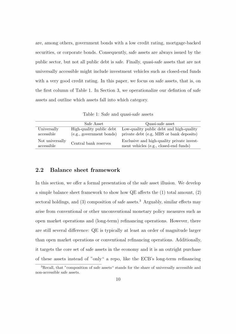
that are not. Table 1 summarizes our taxonomy. Differences in the accessibility

of safe assets are the main driver behind the safe asset illusion. The classical

example for a universally accessible safe asset are government bonds, such as U.S.

Treasuries or German Bunds. Reserves on the other hand are safe, but they are

not universally accessible. Examples for universally accessible quasi-safe assets

9

are, among others, government bonds with a low credit rating, mortgage-backed

securities, or corporate bonds. Consequently, safe assets are always issued by the

public sector, but not all public debt is safe. Finally, quasi-safe assets that are not

universally accessible might include investment vehicles such as closed-end funds

with a very good credit rating. In this paper, we focus on safe assets, that is, on

the first column of Table 1. In Section 3, we operationalize our defintion of safe

assets and outline which assets fall into which category.

Table 1: Safe and quasi-safe assets

Safe Asset Quasi-safe assetUniversallyaccessible

High-quality public debt(e.g., government bonds)

Low-quality public debt and high-qualityprivate debt (e.g, MBS or bank deposits)

Not universallyaccessible

Central bank reservesExclusive and high-quality private invest-ment vehicles (e.g., closed-end funds)

2.2 Balance sheet framework

In this section, we offer a formal presentation of the safe asset illusion. We develop

a simple balance sheet framework to show how QE affects the (1) total amount, (2)

sectoral holdings, and (3) composition of safe assets.3 Arguably, similar effects may

arise from conventional or other unconventional monetary policy measures such as

open market operations and (long-term) refinancing operations. However, there

are still several difference: QE is typically at least an order of magnitude larger

than open market operations or conventional refinancing operations. Additionally,

it targets the core set of safe assets in the economy and it is an outright purchase

of these assets instead of ”only“ a repo, like the ECB’s long-term refinancing

3Recall, that ”composition of safe assets“ stands for the share of universally accessible andnon-accessible safe assets.

10

operations.

Our economy consists of three sectors: the central bank, a banking sector, and

a non-bank sector. The distinguishing feature between a bank and non-bank is the

access to the balance sheet of the central bank. Hence, what we mean by a bank is

any institution with an account at the central bank. This might include entities

without a banking license. In the U.S., for instance, some government-sponsored

enterprises and money market funds have access to the Federal Reserve. Similarly,

we define non-banks as institutions that do not have access to the balance sheet of

the central bank. This includes households, non-financial corporations, insurance

companies, money market funds (in the euro area), hedge funds, pension funds,

etc. In particular, also foreign banks fall into that category.

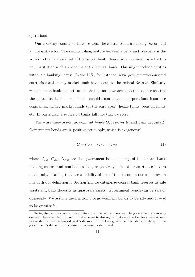
There are three assets: government bonds G, reserves R, and bank deposits D.

Government bonds are in positive net supply, which is exogenous:4

G = GCB +GBA +GNB, (1)

where GCB, GBA, GNB are the government bond holdings of the central bank,

banking sector, and non-bank sector, respectively. The other assets are in zero

net supply, meaning they are a liability of one of the sectors in our economy. In

line with our definition in Section 2.1, we categorize central bank reserves as safe

assets and bank deposits as quasi-safe assets. Government bonds can be safe or

quasi-safe. We assume the fraction ρ of government bonds to be safe and (1− ρ)

to be quasi-safe.

4Note, that in the classical macro literature, the central bank and the government are usuallyone and the same. In our case, it makes sense to distinguish between the two because—at leastin the short run—the central bank’s decision to purchase government bonds is unrelated to thegovernment’s decision to increase or decrease its debt level.

11

Figure 1 presents stylized balance sheets of our sectors. As government bonds

are in positive net supply, they are held as an asset by all three sectors. The central

bank issues reserves, which can only be held by the banking sector. The banking

sector issues unsecured deposits that are held by the non-bank sector.

Figure 1: Sectoral balance sheets

Figure 1 shows the balance sheet of the central bank, the banking sector, and the non-bank sector.

The balance sheets of the central bank, banking sector, and non-bank sector

can be written as:

CB : GCB = R + ECB, (2)

BA : GBA +R = D + EBA (3)

NB : GNB +D = ENB. (4)

Based on this framework, we examine the effects of large-scale government bond

purchases by the central bank on the holdings of safe and quasi-safe assets across

the different sectors.

Figure 2 illustrates the impact of QE on the sectoral balance sheets. The central

bank purchases government bonds from the banking and non-bank sector in the

12

secondary market against reserves, i.e., ∆R = ∆GCB. For simplicity, we assume

that the total amount of government debt G is unaffected by these purchases, i.e.,

∆G = 0. Consequently, the increase in bond holdings at the central bank has to be

offset by a decrease in the holdings of the banking and/or non-bank sector. We

assume that a fraction γ of the purchased bonds comes from the banking sector and

1− γ from the non-bank sector. The variable γ is a reduced-form parameter that

reflects the preferences of banks and non-banks to hold government bonds.5 Using

the budget constraint, Equation (1), we can write: ∆R = γ∆GCB + (1− γ)∆GCB.

Figure 2: Sectoral balance sheets during QE

Figure 2 shows how the balance sheets of the central bank, the banking sector, and the non-banksector are affected through government bond purchases by the central bank.

Figure 2 highlights several interesting facts: First, the central bank extends its

balance sheet by purchasing ∆GCB government bonds using newly created reserves

∆R. Second, the banking sector receives 100% of the newly created reserves. Hence,

for any γ < 1, the balance sheet of the banking sector increases as a consequence

of QE. Third, the non-bank sector sells (1− γ)∆GCB government bonds through

5The term preference should be taken in a broad sense. It encompasses the willingness butalso the requirement to hold safe assets; for example, laws and regulations might prescribe toinvest a certain amount in government bonds.

13

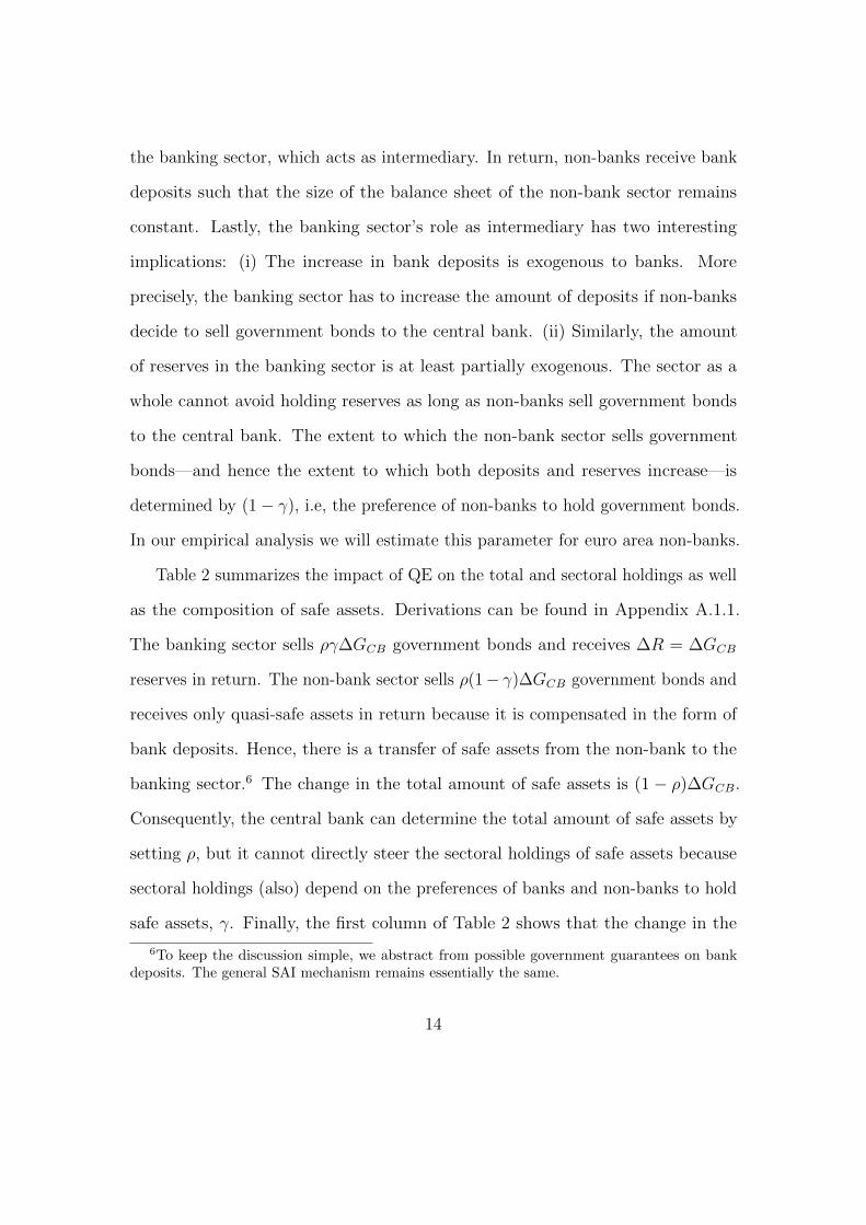
the banking sector, which acts as intermediary. In return, non-banks receive bank

deposits such that the size of the balance sheet of the non-bank sector remains

constant. Lastly, the banking sector’s role as intermediary has two interesting

implications: (i) The increase in bank deposits is exogenous to banks. More

precisely, the banking sector has to increase the amount of deposits if non-banks

decide to sell government bonds to the central bank. (ii) Similarly, the amount

of reserves in the banking sector is at least partially exogenous. The sector as a

whole cannot avoid holding reserves as long as non-banks sell government bonds

to the central bank. The extent to which the non-bank sector sells government

bonds—and hence the extent to which both deposits and reserves increase—is

determined by (1− γ), i.e, the preference of non-banks to hold government bonds.

In our empirical analysis we will estimate this parameter for euro area non-banks.

Table 2 summarizes the impact of QE on the total and sectoral holdings as well

as the composition of safe assets. Derivations can be found in Appendix A.1.1.

The banking sector sells ργ∆GCB government bonds and receives ∆R = ∆GCB

reserves in return. The non-bank sector sells ρ(1− γ)∆GCB government bonds and

receives only quasi-safe assets in return because it is compensated in the form of

bank deposits. Hence, there is a transfer of safe assets from the non-bank to the

banking sector.6 The change in the total amount of safe assets is (1 − ρ)∆GCB.

Consequently, the central bank can determine the total amount of safe assets by

setting ρ, but it cannot directly steer the sectoral holdings of safe assets because

sectoral holdings (also) depend on the preferences of banks and non-banks to hold

safe assets, γ. Finally, the first column of Table 2 shows that the change in the

6To keep the discussion simple, we abstract from possible government guarantees on bankdeposits. The general SAI mechanism remains essentially the same.

14

total amount of safe assets is composed of an increase in non-universally accessible

safe assets and a decrease in universally accessible safe assets. The former increase

by ∆R = ∆GCB and the latter decrease by ρ∆GCB.

Table 2 also presents the changes of the total and sectoral holdings of quasi-safe

asset. The holdings of the banking sector decrease by (1 − ρ)γ∆GCB, i.e., the

amount of quasi-safe government bonds sold by banks. In case of the non-bank

sector, the quasi-safe asset holdings increase by ρ(1− γ)∆GCB, i.e., the amount of

safe government bonds sold. This is due to the fact that non-banks only receive

bank deposits when selling safe government bonds. Additionally, the quasi-safe

asset holdings of non-banks do not change if they sell quasi-safe government bonds

because such a transaction would simply be a swap of two quasi-safe assets (quasi-

safe government bonds against bank deposits). In sum, whether the total amount

of quasi-safe assets increases or decreases depends on the relative size of the policy

parameter ρ that is determined by the central bank and the preference parameter

γ that differs across economic agents.7 The more safe assets are purchased by

the central bank (high ρ) and from the non-bank sector (small γ), the higher the

increase of quasi-safe assets.

In order to derive a measure for the preference of different sectors s to hold

government bonds, we introduce γs, where s ∈ {Bank, ICPF, OFI, HH, Other,

Foreign} and∑

s γs = 1.8 Against this background, we use

∆Gssafe

Gssafe

= −ργs∆GCB

Gssafe

(5)

7In the euro area, ρ is determined by the ECB capital key of the individual member countries.8Insurance companies and pension funds (ICPF), other financial institutions (OFI), households

(HH), others (Other), and foreign institutions (Foreign) are the non-bank sectors in our data,which we introduce in more detail in Section 3.

15

Table 2: Change in total and sectoral holdings of (quasi-)safe assets

Table 2 presents the changes in total and sectoral holdings of safe and quasi-safe assets. Derivationscan be found in the Appendix.

Safe assets Quasi-safe assetsBanking sector (1− ργ)∆GCB −(1− ρ)γ∆GCB

Non-bank sector −ρ(1− γ)∆GCB ρ(1− γ)∆GCB

Total (1− ρ)∆GCB (ρ− γ)∆GCB

as a measure for the cross-sectional variation in the preference to hold safe govern-

ment bonds. We can do this because the only driver of cross-sectional variation in

this measure is variation in γs. When bringing this measure to the data, we still

need to correct for the fact that the amount of outstanding government bonds also

changes due to the issuance of new bonds. We derive this measure in an extension

of the framework in the Appendix. While adding the issuance of new government

bonds to the framework is necessary to make it fully transparent how our measure

can be brought to SHSS data, nothing changes from a conceptual point of view.

Since the extension adds some complexity without changing the overall picture, we

decided to move it to the appendix.

We can now use the results presented in Table 2 to derive conditions for the

neutrality of QE for (1) the total amount, (2) the sectoral holdings, and (3) the

composition of safe assets.

Proposition 1 (Safe asset neutrality of QE)

(i) QE is neutral to the total amount of safe assets if ρ = 1, i.e., if the central

bank purchases only safe government bonds.

(ii) QE is neutral to the sectoral holdings of safe assets if ρ = γ = 1, i.e., if the

16

central bank purchases only safe government bonds and only from banks.

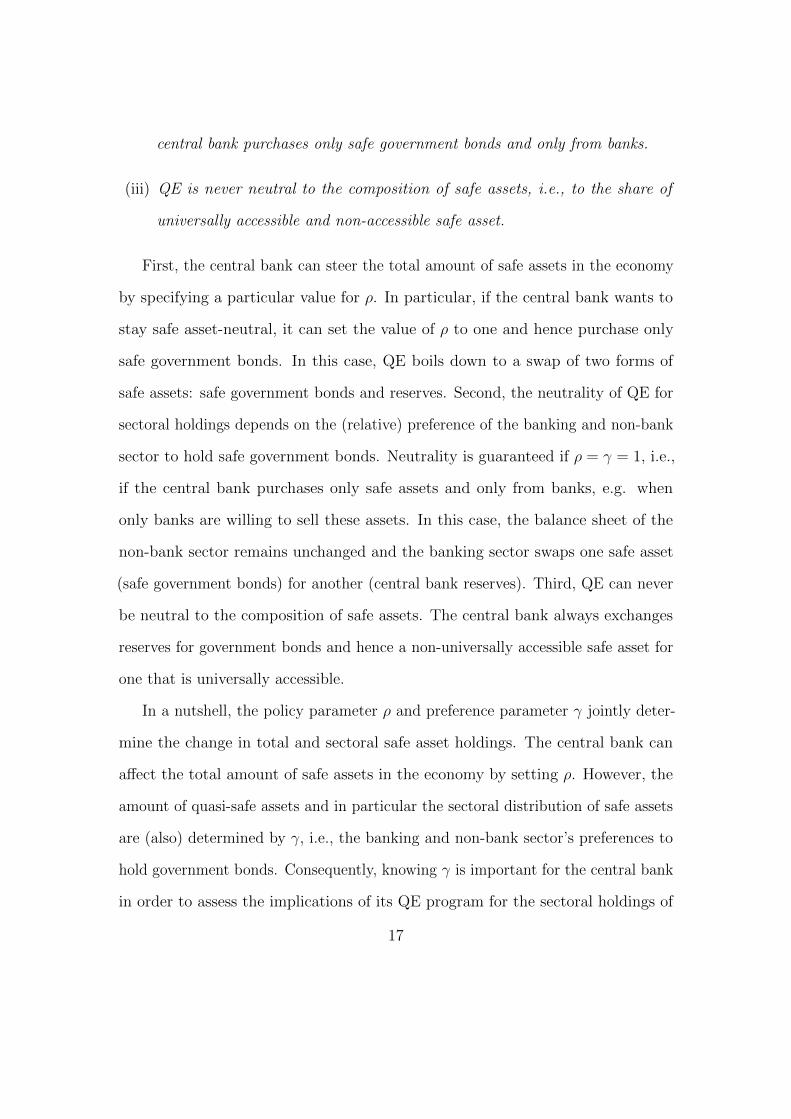
(iii) QE is never neutral to the composition of safe assets, i.e., to the share of

universally accessible and non-accessible safe asset.

First, the central bank can steer the total amount of safe assets in the economy

by specifying a particular value for ρ. In particular, if the central bank wants to

stay safe asset-neutral, it can set the value of ρ to one and hence purchase only

safe government bonds. In this case, QE boils down to a swap of two forms of

safe assets: safe government bonds and reserves. Second, the neutrality of QE for

sectoral holdings depends on the (relative) preference of the banking and non-bank

sector to hold safe government bonds. Neutrality is guaranteed if ρ = γ = 1, i.e.,

if the central bank purchases only safe assets and only from banks, e.g. when

only banks are willing to sell these assets. In this case, the balance sheet of the

non-bank sector remains unchanged and the banking sector swaps one safe asset

(safe government bonds) for another (central bank reserves). Third, QE can never

be neutral to the composition of safe assets. The central bank always exchanges

reserves for government bonds and hence a non-universally accessible safe asset for

one that is universally accessible.

In a nutshell, the policy parameter ρ and preference parameter γ jointly deter-

mine the change in total and sectoral safe asset holdings. The central bank can

affect the total amount of safe assets in the economy by setting ρ. However, the

amount of quasi-safe assets and in particular the sectoral distribution of safe assets

are (also) determined by γ, i.e., the banking and non-bank sector’s preferences to

hold government bonds. Consequently, knowing γ is important for the central bank

in order to assess the implications of its QE program for the sectoral holdings of

17

safe assets. In the Appendix, we discuss several boundary cases for ρ and γ.

3 Empirical analysis

In this section, we bring our balance sheet framework to data from the euro area

in order to examine the (non-)neutrality of the PSPP for safe assets and quantify

the effects. We measure changes in total and sectoral holdings of safe assets as well

as their composition between March 2015 and December 2018.

3.1 Public Sector Purchase Programme

The PSPP was formally announced in January 2015 and further implementation

details were communicated in March 2015, which marks also the start date of the

large scale asset purchase program of the euro area. The policy rationale of the

PSPP was to provide additional monetary policy accommodation in a situation in

which policy rates could not be cut (much) further (the deposit facility rate had

reached a level of −0.20 percent and the main refinancing rate stood at 0 percent).

The initial monthly envelope of PSPP purchases was EUR 60 billion, which

was increased in April 2016 to EUR 80 billion and then decreased again to EUR 60

billion in April 2017. Between March 2015 and December 2018, the Eurosystem

has purchased EUR 2.2 trillion of euro area government bonds, agency bonds and

euro area supras (e.g., EIB bonds).9 The purchase volumes were split according

to the capital key. In other words, each national central bank of the Eurosystem

purchased the share of the monthly PSPP envelope that corresponds to its capital

9Cumulative net purchase figures in this sub-section represent the difference between theacquisition cost of all purchase operations and the redeemed nominal amounts.

18

share, exclusively focusing on the govenment bonds of their own country.

As of 31 December 2018, out of the total PSPP purchase volume, the Eurosystem

had acquired EUR 519 billion in German, EUR 420 billion in French, EUR 365

billion in Italian, EUR 261 billion in Spanish and EUR 115 billion in Dutch

public sector bonds, corresponding to 26.1%, 18.3%, 16.9%, 21.8%, 24.5% of all

outstanding bonds of these countries.

3.2 Data description

We use data from the Securities Holdings Statistics by Sector (SHSS) database

which provides information on holdings of securities by euro area resident sectors.

In our sample, debt securities are identified by a unique International Securities

Identifier Number (ISIN) and the total reported holdings of these securities per

quarter are approximately EUR 19 trillion in nominal value. We merge the SHSS

data with the nominal value of the asset purchase programme (APP) holdings

of the Eurosystem at the security level and quarterly frequency, amounting to a

total of around EUR 2.4 trillion in Q4 2018. In addition, we enrich the database

with security level characteristics and outstanding amounts from the Centralised

Securities Database (CSDB), and complement the CSDB data with data on credit

ratings given by DBRS, Fitch, Moodys and Standard and Poors. When no sovereign-

and ISIN-level credit ratings are available, we use issuer-level credit ratings based

on characteristics of the ISINs. Our sample spans from Q2 2014 until Q4 2018.

Following Koijen et al. (2020), we group the SHSS holdings sectors into five

euro area sectors: monetary financial institutions (MFI, or: Banks), insurance

corporations and pensions funds (ICPF), other financial institutions (OFI) which

19

includes money market funds, investment funds and other financial corporations,

households (HH), and government and non-financial corporations (Other). We also

add the Eurosystem sector characterised by the APP holdings. Finally we create

the foreign sector (Foreign)—that is, non-euro area investors—as the residual

obtained from the difference between the total outstanding amount of a given

security and the aggregate holdings of the corresponding security by euro area

sectors.10 In addition, as CSDB should cover the full universe of euro-denominated

securities issued by euro area entities, we assign the total outstanding amount of

those securities of interest not included in the SHSS to the foreign sector.

We distinguish the assets covered in our sample between both government and

corporate bonds, asset-backed securities and covered bonds. For the purpose of

our analysis, we focus on euro-denominated government debt securities issued by

euro area legal entities, including agency bonds and supras held under the PSPP.

To this end, we use the CSDB characteristics to filter out securities that are still

alive in the investors’ holdings portfolio and classify them according to their debt

type.11 Thus, total nominal holdings of government debt securities amount to

approximately EUR 8.3 trillion on average over our review period. In addition,

holdings by the Eurosystem sector only comprise the PSPP purchases.

10A shortcoming of the SHSS data is the difficulty of measuring securities positions of investorslocated outside the euro area—also known as custodial bias—as foreign holdings are reported toa large extent indirectly via euro area custodians which may then not pick up the country of thefinal investor. Thus, holdings by the foreign sector are treated as a residual category to matchthe aggregate outstanding nominal amount of the securities of interest.

11Securities that have not been redeemed yet, but have a negative residual maturity, can still bereported in the investors’ holdings portfolio. We do not include securities with negative residualmaturity according to CSDB.

20

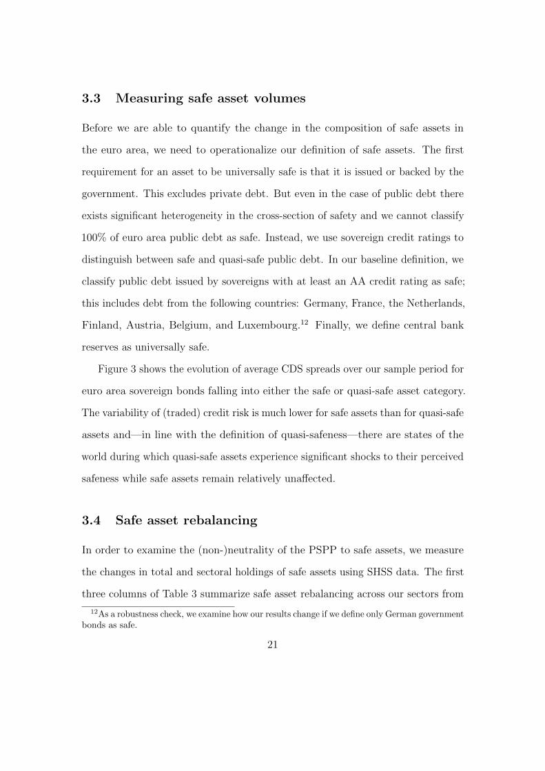
3.3 Measuring safe asset volumes

Before we are able to quantify the change in the composition of safe assets in

the euro area, we need to operationalize our definition of safe assets. The first

requirement for an asset to be universally safe is that it is issued or backed by the

government. This excludes private debt. But even in the case of public debt there

exists significant heterogeneity in the cross-section of safety and we cannot classify

100% of euro area public debt as safe. Instead, we use sovereign credit ratings to

distinguish between safe and quasi-safe public debt. In our baseline definition, we

classify public debt issued by sovereigns with at least an AA credit rating as safe;

this includes debt from the following countries: Germany, France, the Netherlands,

Finland, Austria, Belgium, and Luxembourg.12 Finally, we define central bank

reserves as universally safe.

Figure 3 shows the evolution of average CDS spreads over our sample period for

euro area sovereign bonds falling into either the safe or quasi-safe asset category.

The variability of (traded) credit risk is much lower for safe assets than for quasi-safe

assets and—in line with the definition of quasi-safeness—there are states of the

world during which quasi-safe assets experience significant shocks to their perceived

safeness while safe assets remain relatively unaffected.

3.4 Safe asset rebalancing

In order to examine the (non-)neutrality of the PSPP to safe assets, we measure

the changes in total and sectoral holdings of safe assets using SHSS data. The first

three columns of Table 3 summarize safe asset rebalancing across our sectors from

12As a robustness check, we examine how our results change if we define only German governmentbonds as safe.

21

Figure 3: CDS rates of safe and quasi-safe assets

Figure 3 presents average CDS rates of safe and quasi-safe assets in the euro area.

Q1 2015 to Q4 2018. The first column shows the cumulative changes in reserve

holdings of the banking sector as a share of euro area GDP. Reserve holdings

increases strongly because banks receive reserves irrespective of which sector sells

safe and quasi-safe government bonds to the ECB.13

The second column summarizes the rebalancing of safe government bonds as

a share of euro area GDP. The ECB purchases 11.1% of safe government bonds

from the banking and non-bank sector. Banks decrease their holdings by 3.4% and

non-banks by 4.4%, leading to a total reduction in safe government bonds of 7.8%.

The difference between this reduction and the ECB purchases amounts to 3.3%,

which is the positive net issuance of additional safe government bonds by euro

13Since the PSPP has not been the only purchase program and since there are other drivers ofreserve holdings, the change in reserves deviates from the total PSPP purchase volume (14.3% vs.16.7% as a share of euro area GDP). Hence, the assumption ∆R = ∆G from the balance sheetmodel does not hold and therefore we use the change in reserve holding ∆R directly to measurethe change in safe asset holdings.

22

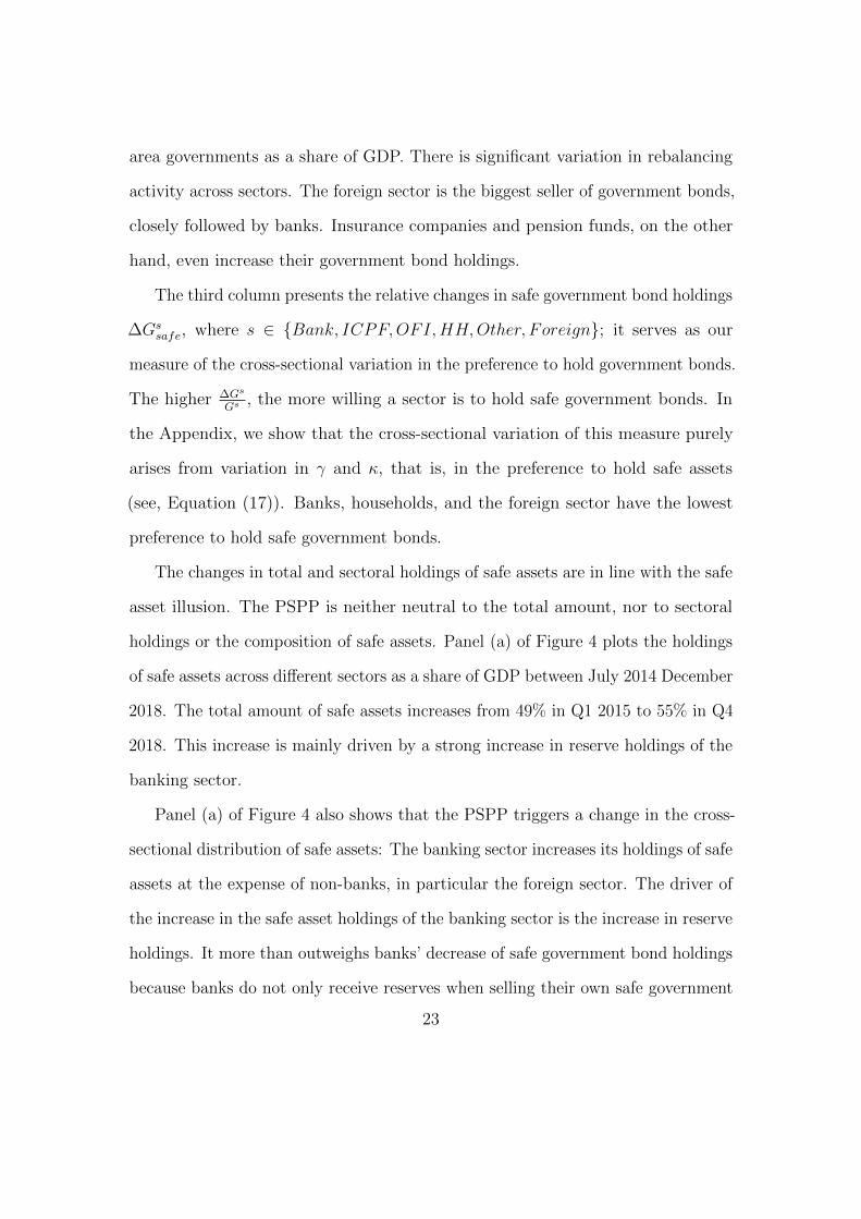
area governments as a share of GDP. There is significant variation in rebalancing

activity across sectors. The foreign sector is the biggest seller of government bonds,

closely followed by banks. Insurance companies and pension funds, on the other

hand, even increase their government bond holdings.

The third column presents the relative changes in safe government bond holdings

∆Gssafe, where s ∈ {Bank, ICPF,OFI,HH,Other, Foreign}; it serves as our

measure of the cross-sectional variation in the preference to hold government bonds.

The higher ∆Gs

Gs , the more willing a sector is to hold safe government bonds. In

the Appendix, we show that the cross-sectional variation of this measure purely

arises from variation in γ and κ, that is, in the preference to hold safe assets

(see, Equation (17)). Banks, households, and the foreign sector have the lowest

preference to hold safe government bonds.

The changes in total and sectoral holdings of safe assets are in line with the safe

asset illusion. The PSPP is neither neutral to the total amount, nor to sectoral

holdings or the composition of safe assets. Panel (a) of Figure 4 plots the holdings

of safe assets across different sectors as a share of GDP between July 2014 December

2018. The total amount of safe assets increases from 49% in Q1 2015 to 55% in Q4

2018. This increase is mainly driven by a strong increase in reserve holdings of the

banking sector.

Panel (a) of Figure 4 also shows that the PSPP triggers a change in the cross-

sectional distribution of safe assets: The banking sector increases its holdings of safe

assets at the expense of non-banks, in particular the foreign sector. The driver of

the increase in the safe asset holdings of the banking sector is the increase in reserve

holdings. It more than outweighs banks’ decrease of safe government bond holdings

because banks do not only receive reserves when selling their own safe government

23

Table 3: Safe asset rebalancing

Table 3 shows the cumulative rebalancing as a share of euro area real GDP (in percent) fromQ1 2015 to Q4 2018 of safe assets (reserves and government bonds rated at least AA), Germangovernment bonds, and government bonds rated lower than AA. The third, fifth, and seventhcolumn present relative changes (in percent), which serve as a proxy for the cross-sectionalvariation in the preference of holing these assets. The top panel reports the rebalancing of thebanking and non-bank sector, distinguishing between the five non-bank categories. The secondpanel reports the rebalancing of the Eurosystem and the bottom panel reports net issuances.

Safe assets Gov bonds (DE) Gov bonds (<AA)

Sector ∆ RGDP

∆ Gs

GDP∆Gs

Gs ∆ Gs

GDP∆Gs

Gs ∆ Gs

GDP∆Gs

Gs

Banks 14.33 −3.42 −30.89 −1.31 −32.98 −1.22 −6.95

Non-banks −4.43 −4.77 −1.59 −5.16 −1.77 −1.92

OFI −0.07 6.76 −0.10 2.04 −1.11 −14.93

ICPF 0.65 16.46 0.14 21.53 0.88 25.33

HH −0.12 −39.54 −0.07 −44.18 −0.47 −19.49

Other −0.07 3.91 0.00 8.68 −0.39 −19.48

Foreign −4.83 −16.27 −1.56 −10.82 −0.68 −7.07

Eurosystem 11.10 4.01 5.60Total 14.33 3.26 1.11 2.61

bonds, but also when selling their quasi-safe bonds and when selling bonds for their

customers. The holdings of insurance companies and pension funds remain stable.

The holdings of households and other non-bank entities are negligible.

Finally, Panel (b) of Figure 4 shows that the PSPP also affects the composition

of safe assets. It presents the holdings of universally accessible safe assets. The

total amount of these assets decreases from 46% of euro area GDP in Q1 2015 to

39% in Q4 2018. Consequently, the amount of safe assets that are not universally

accessible (that is, reserves) increases at the expense of universally accessible safe

24

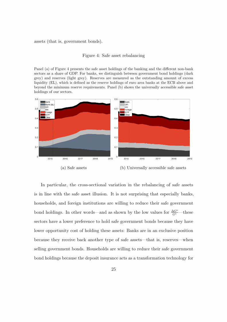
assets (that is, government bonds).

Figure 4: Safe asset rebalancing

Panel (a) of Figure 4 presents the safe asset holdings of the banking and the different non-banksectors as a share of GDP. For banks, we distinguish between government bond holdings (darkgrey) and reserves (light grey). Reserves are measured as the outstanding amount of excessliquidity (EL), which is defined as the reserve holdings of euro area banks at the ECB above andbeyond the minimum reserve requirements. Panel (b) shows the universally accessible safe assetholdings of our sectors.

(a) Safe assets (b) Universally accessible safe assets

In particular, the cross-sectional variation in the rebalancing of safe assets

is in line with the safe asset illusion. It is not surprising that especially banks,

households, and foreign institutions are willing to reduce their safe government

bond holdings. In other words—and as shown by the low values for ∆Gs

Gs —these

sectors have a lower preference to hold safe government bonds because they have

lower opportunity cost of holding these assets: Banks are in an exclusive position

because they receive back another type of safe assets—that is, reserves—when

selling government bonds. Households are willing to reduce their safe government

bond holdings because the deposit insurance acts as a transformation technology for

25

them, transforming a quasi-safe asset into a safe asset (up to 100,000 EUR, which

is a meaningful size for the average household). Finally, the trade-off for the foreign

sector is of a somewhat different nature because safe euro area government bonds

can be replaced by a similar safe government bond from another jurisdiction—for

example, US treasuries—without fundamentally changing the risk profile of the

asset.

3.5 Robustness checks

The fourth and fifth column of Table 3 present the rebalancing volumes for German

government bonds.14 These numbers serve as a robustness check to examine if our

results change when applying a more restrictive definition of safe assets. The cross-

sectional variation of the preferences to hold safe government bonds—measured by

∆Gs

Gs —is similar to our baseline results. Banks, households, and the foreign sector

are most willing to reduce their safe government bond holdings.

The sixth and seventh column of Table 3 present the reblancing volumes for

quasi-safe government bonds, that is, bonds rated lower than AA. The cross-

sectional variation in the preferences to hold these bonds differs from our baseline

results. Except for insurance companies and pension funds, which increase their

holdings of quasi-safe bonds, all other sectors reduce their holdings. These results

support our approach to measuring safe and quasi-safe assets using AA as a rating

threshold. There seems to be a difference in the rebalancing behavior between

government bonds with ratings above and below this threshold.

14German government bonds follow the same definition as overall government bonds, includingGerman agency bonds held under the PSPP.

26

4 Implications of the safe asset illusion

In this section, we discuss two main implications of the safe asset illusion: First, we

analyze the premium that non-banks have to pay for safely storing their liquidity.

There are two main ways to safely store liquidity: central bank reserves and general

collateral (GC) repurchase agreements (repos). While banks can rely on both,

non-banks cannot access the central bank deposit facility and therefore they have

to pay a premium to ensure that their liquidity is stored safely. Second, we show

that the PSPP reduces the collateral quality in the money market, which may

adversely impact financial stability.

4.1 Distributional consequences for the banking and non-

bank sector: safe storage premium

The GC repo market with safe assets as collateral is one of very few—if not the

only—possibilities for non-banks to deposit their short-term liquidity nearly without

risk.15 A GC repo is conceptually identical to a (very) short-term secured loan.

Hence, the cash-rich agent lends its funds to (or deposits with) a cash-seeking agent

at a predefined rate and maturity against collateral.

Since the start of the PSPP, however, the repo rate has fallen strongly, in

particular for repos backed by safe assets. Extant literature suggests that large-

scale government bond purchases render safe assets scarce, which is reflected in

15There are other financial instruments for holding liquid positions such as certificates of depositand savings or money market accounts. However, (reverse) repos secured by safe assets representthe safest option for lending with very short maturities. The asset being used as collateral can bea particular asset (special collateral or SC repos) or any asset from a predefined basket of assets(general collateral or GC repos). We focus on GC repos because this is the market segment thatis used to manage liquidity, while SC repos are rather used to borrow or lend securities.

27

lower rates for these assets in the repo market (e.g., D’Amico, Fan, and Kitsul,

2018; Arrata et al., 2020; Corradin and Maddaloni, 2020). Therefore, it has become

more and more expensive to store short-term liquidity safely. For banks, the

deposit facility rate (DFR) is a lower bound for the rate they accept to deposit

their cash. Hence, if the repo rate drops below the DFR, banks have a strong

incentive to deposit their cash at the deposit facility instead of using the repo

market. Non-banks on the other hand do not have access to this facility. Their

main alternative to a bank deposit is the repo market, which increases their safe

storage cost relative to that of banks, creating a safe storage premium. This

premium can be interpreted as a convenience yield that originates due to a market

segmentation in the market for reserves. The safe asset literature points to two

main determinants of the convenience yield: a safety and a liquidity premium

(e.g., Krishnamurthy and Vissing-Jorgensen, 2012; Sunderam, 2015; Gorton, 2017),

which in turn increases with the opportunity cost of holding money (Nagel, 2016).

The segmentation inherent in the monetary policy setting granting the access only

to banks induces non-banks to pay a convenience yield for holding liquidity safely.

Figure 5 plots the rate on the ECB’s deposit facility together with the overnight

rate on euro GC repos backed by safe euro area government bonds (blue) and

German government bonds (black).16 In an overnight GC repo, the non-bank

deposits cash overnight in return for a government bond. The transaction is

reversed the next day. Both the DFR and GC repo rate have moved to negative

territory already in 2014. Additionally, the repo rate has dropped below the DFR

shortly after the start of the PSPP and stayed there ever since. Hence, since at

16We collect the underlying data from the three major repo exchanges in the euro area:BrokerTec, Eurex, and MTS. For a more detailed description of the market and this dataset, seeRanaldo, Schaffner, and Vasios (2020).

28

least mid-2015 non-banks have to pay a premium to store their overnight liquidity

safely. Between March 2015 and December 2018, this premium has averaged 7

basis points for safe government bonds and 10 basis points for German government

bonds.

These costs likely represent a lower bound estimate for the costs of non-banks for

a GC repo as these rates are those observed on large platforms which typically do

not have non-banks among their customers. Eisenschmidt, Ma, and Zhang (2020)

show that non-banks can access the repo market only at significantly higher costs

than banks. Looking at repo rates in the OTC segment contained in the ECB’s

MMSR statistic allows separating repo trades according to their counterparty. Repo

spreads paid by non-banks are significantly higher than those paid by banks, with

non-banks paying between 10 – 15 basis points higher rates than banks, although

the drawback of the approach is that a clean separation between GC and SC repos

is not possible and the estimated spread between non-banks and banks may be

biased upwards. In any case, the reported premia are substantial given the very

low interest rates in the money market. If banks had to store their liquidity in the

GC repo market, that is, they would have to pay a similar type of premium as

non-banks to safely store their reserves, they would have faced additional cost of

EUR 3.3 – 4.7 billion between March 2015 and December 2018.17 Consequently,

the market segmentation in the market for central bank reserves creates a wedge

between the banking and non-bank sector when it comes to the costs of safely

storing cash.

17Computed as average amount of excess liquidity times 7 basis points (lower bound) and 10basis points (upper bound) annualized interest rate spread for the period March 2015 – December2018. Recall that excess liquidity is defined as the reserve holdings of euro area banks at the ECBabove and beyond the minimum reserve requirements.

29

Figure 5: The safe storage premium

Figure 5 plots the rate on the ECB’s deposit facility rate together with the rate on general collateralrepurchase agreements backed by safe government bonds (blue) and German government bonds(black). The dotted vertical line marks the start of the PSPP purchases in March 2015.

4.2 Fragile liquidity

In this section, we show that due to the PSPP, the overall quality of collateral in the

money market decreases. The rationale behind this development is straight-forward:

With the start of the PSPP, the share of universally accessible safe assets steadily

decreases because the ECB acts as buy and hold investor of safe government bonds.

In particular, the ECB purchases more safe than quasi-safe government bonds (in

absolut and relative terms). This reduction in the relative supply of safe government

bonds is reflected in the use of these assets as collateral in the money market. The

consequent substitution from safe to quasi-safe collateral is important because it

contributes to financial fragility.

Figure 6 plots the trading volume of overnight euro GC repos traded on the

three major exchanges in the euro area (BrokerTec, Eurex, and MTS). The figure

distinguishes between repos backed by safe and quasi-safe government bonds. Before

30

the start of the PSPP purchases—indicated by the dotted vertical line—cumulated

trading volumes of repos backed by quasi-safe assets were slightly below those

backed by safe assets. After the start of the PSPP, repo volumes start to fall

because of the additional excess liquidity in the system. However, trading volumes

of repos backed by safe assets fall faster than those backed by quasi-safe assets.

Thereby the collateral base in the repo market deteriorates, increasing the share of

quasi-safe assets.

Figure 6: GC repo trading volumes

Figure 6 plots the repo trading volume of overnight euro GC repos collateralized by safe andquasi-safe assets. The data captures repos traded on the three major trading platforms in Europe:BrokerTec, Eurex, and MTS. The dotted vertical line marks the start of the PSPP purchases.

As discussed above, quasi-safe assets behave similarly to safe assets during

normal times and even carry a convenience premium (e.g., Kacperczyk, Perignon,

and Vuillemey, 2018). However, their convenience yield is wobbling because in bad

times, their safety and liquidity attributes reduce or can even disappear swiftly.

The main issue is that quasi-safe assets become information-sensitive as investors

doubt the true value and risk of these assets. This mechanism also applies to

31

quasi-safe assets used as collateral impairing their collateral value. Against this

background, a collateral base consisting of a high share of quasi-safe assets leads

to financial fragility (Gorton and Ordonez, 2014) or fragile liquidity (Moreira and

Savov, 2017).

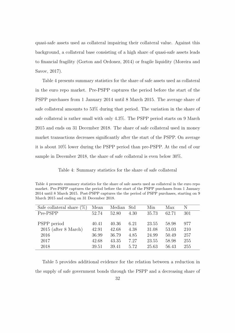
Table 4 presents summary statistics for the share of safe assets used as collateral

in the euro repo market. Pre-PSPP captures the period before the start of the

PSPP purchases from 1 January 2014 until 8 March 2015. The average share of

safe collateral amounts to 53% during that period. The variation in the share of

safe collateral is rather small with only 4.3%. The PSPP period starts on 9 March

2015 and ends on 31 December 2018. The share of safe collateral used in money

market transactions decreases significantly after the start of the PSPP. On average

it is about 10% lower during the PSPP period than pre-PSPP. At the end of our

sample in December 2018, the share of safe collateral is even below 30%.

Table 4: Summary statistics for the share of safe collateral

Table 4 presents summary statistics for the share of safe assets used as collateral in the euro repomarket. Pre-PSPP captures the period before the start of the PSPP purchases from 1 January2014 until 8 March 2015. Post-PSPP captures the the period of PSPP purchases, starting on 9March 2015 and ending on 31 December 2018.

Safe collateral share (%) Mean Median Std Min Max NPre-PSPP 52.74 52.80 4.30 35.73 62.71 301

PSPP period 40.41 40.36 6.21 23.55 58.98 9772015 (after 8 March) 42.91 42.68 4.38 31.08 53.03 2102016 36.99 36.79 4.85 24.99 50.49 2572017 42.68 43.35 7.27 23.55 58.98 2552018 39.51 39.41 5.72 25.63 56.43 255

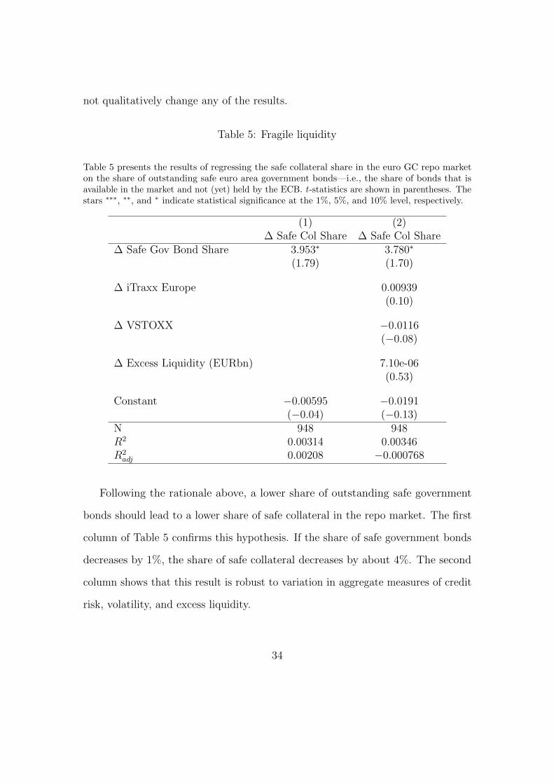
Table 5 provides additional evidence for the relation between a reduction in

the supply of safe government bonds through the PSPP and a decreasing share of

32

safe collateral in the euro GC repo market. It presents the results of the following

regression:

∆Safe Col Share = α + β∆Safe Gov Bond Share

+ γ1∆iT raxxt + γ2∆V STOXXt + γ3∆ELt + εt,

(6)

where Safe Col Share is the safe collateral share in the euro GC repo market(V olSA

t

V olTotalt

), Safe Gov Bond Share is the share of outstanding safe euro area govern-

ment bonds, that is, the share of bonds that is available in the market and not

(yet) held by the ECB(

OutstandingSAt

OutstandingTotalt

). iT raxxt is the iTraxx Europe. It captures

variation in CDS spreads that might be caused by changes in market-wide credit

or liquidity risk. V STOXXt captures changes in expectations about aggregate

volatility. It reflects the investor sentiment and overall economic uncertainty by

measuring the 30-day implied volatility of the EURO STOXX 50. ELt is the

level of excess liquidity holdings. Including ELt enables us to control for potential

changes in the demand for safe collateral that are driven by the need to safely store

the additional liquidity from the PSPP. Finally, εt is the error term. In order to

ensure stationarity and to rule out spurious correlation, we take first differences of

all variables. Additionally, we estimate Equation (6) using robust standard errors.

Since GC repo baskets only exist for selected euro area countries, we consider

only the following countries in this analysis: Austria, Belgium, Germany, Finland,

France, Luxembourg, the Netherlands (safe) and Spain, Greece, Ireland, and

Portugal (quasi-safe). In order to control for end-of-quarter effects and eliminate

problems stemming from extreme seasonalities common to repo markets, we exclude

the last day of each quarter from the regression. Leaving these observations in does

33

not qualitatively change any of the results.

Table 5: Fragile liquidity

Table 5 presents the results of regressing the safe collateral share in the euro GC repo marketon the share of outstanding safe euro area government bonds—i.e., the share of bonds that isavailable in the market and not (yet) held by the ECB. t-statistics are shown in parentheses. Thestars ∗∗∗, ∗∗, and ∗ indicate statistical significance at the 1%, 5%, and 10% level, respectively.

(1) (2)∆ Safe Col Share ∆ Safe Col Share

∆ Safe Gov Bond Share 3.953∗ 3.780∗

(1.79) (1.70)

∆ iTraxx Europe 0.00939(0.10)

∆ VSTOXX −0.0116(−0.08)

∆ Excess Liquidity (EURbn) 7.10e-06(0.53)

Constant −0.00595 −0.0191(−0.04) (−0.13)

N 948 948R2 0.00314 0.00346R2

adj 0.00208 −0.000768

Following the rationale above, a lower share of outstanding safe government

bonds should lead to a lower share of safe collateral in the repo market. The first

column of Table 5 confirms this hypothesis. If the share of safe government bonds

decreases by 1%, the share of safe collateral decreases by about 4%. The second

column shows that this result is robust to variation in aggregate measures of credit

risk, volatility, and excess liquidity.

34

5 Conclusion

We propose a simple balance sheet framework outlining the non-neutrality of large-

scale government bond purchases—known as Quantitative Easing, short: QE—to

safe assets. We show that while QE increases the total amount of safe assets, it

transfers safe assets from the non-bank to the banking sector and it decreases the

amount of safe assets that are universally accessible. We call this phenomenon the

safe asset illusion. In our empirical analysis, we show that during the ECB’s Public

Sector Purchase Programme—between Q1 2015 and Q4 2018—the total amount of

safe assets increases from 49% to 55% of euro area GDP. However, this increase

is exclusively driven by newly issued central bank reserves and only the banking

sector profits from it. The safe asset holdings of the non-bank sector decrease

by 4.4% during the same period. Importantly, the total amount of universally

accessible safe assets decreases from 46% of euro area GDP in Q1 2015 to 39% in

Q4 2018, contributing significantly to the overall scarcity of safe assets in the euro

area. We examine two implications of this safe asset scarcity for the distribution of

wealth and financial stability: First, since non-banks do not have access to central

bank reserves, they have to pay a premium for safely storing their liquidity. Second,

the PSPP deteriorates the collateral quality in the money market.

The main friction behind the safe asset illusion is the market segmentation

originating from granting only the banking sector access to the balance sheet of the

central bank. This gives rise to several possible policy responses that can mitigate

the adverse effects of the safe asset illusion: First, the ECB could extend the access

to its reserves to a wider range of institutions. This would allow (parts of) the

non-bank sector to profit from the possibility to safely and (relatively) cheaply

35

store liquidity in the deposit facility (or a similar facility). Against this background,

the debate around retail central bank digital currencies (CBDC) seems interesting

because a retail CBDC would give all economic agents access to central bank money.

Of course, the implications of a retail CBDC go far beyond its effect on safe assets.

Nevertheless, it seems worth to include this dimension into the debate surrounding

the introduction of a CBDC.

A second policy response to address the adverse effects of the safe asset illusion

would be to increase the availability of universally accessible safe assets. For

instance, the ECB could intensify its efforts to channel back safe assets into the

market via its securities lending facility. Alternatively, it could issue its own safe

assets, for instance, in form of ECB Debt Certificates (Hardy, 2020). Securities

lending as well as ECB Debt Certificates would mitigate the scarcity of safe

collateral in the repo market, leading to higher repo rates. Therefore, these policies

could decrease the cost of safely storing liquidity for the institutions without access

to the deposit facility.

The goal of this paper was to outline and document the effect of QE—in partic-

ular, of the PSPP—on the total amount, sectoral distribution, and composition

of safe assets. Our findings raise a couple of interesting questions, which can

be addressed by future research. For instance: Are banks profiting or suffering

from the additional safe asset holdings? Since excess liquidity is remunerated at

negative interest rates, it is open whether the net effect of additional safe assets is

positive or negative for the banking sector. Moreover, the safe asset illusion suggests

that the cross-sectional heterogeneity in the preferences to hold safe government

bonds have important implications for the transmission efficiency of QE. Especially

those sectors with high opportunity cost of holding safe assets are less willing to

36

give these assets away. Against this background, it seems likely that the ex ante

holding structure of government bonds matters for the efficiency of QE. If most of

the government bonds are in the hands of sectors with a high preference to hold

government bonds, the price impact of asset purchases might increase.

37

References

Arrata, W., B. Nguyen, I. Rahmouni-Rousseau, and M. Vari. 2020. The scarcity

effect of QE on repo rates: evidence from the euro area. Journal of Financial

Economics 137:837–856.

Azzimonti, M., and P. Yared. 2018. The optimal public and private provision of

safe assets. NBER Working Paper 24534.

Barro, R. J., J. Fernandez-Villaverde, O. Levintal, and A. Mollerus. 2017. Safe

Assets. NBER Working Paper 20652:1–46.

Benigno, P., and S. Nistico. 2017. Safe Assets, Liquidity, and Monetary Policy.

American Economic Journal: Macroeconomics 9:182–227.

Caballero, B. R. J., E. Farhi, and P.-O. Gourinchas. 2008. An Equilibrium Model

of “Global Imbalances” and Low Interest Rates. American Economic Review

98:358–393.

Caballero, R. J., and E. Farhi. 2018. The Safety Trap. Review of Economic Studies

85:223–274.

Caballero, R. J., E. Farhi, and P.-O. Gourinchas. 2017. The Safe Assets Shortage

Conundrum. Journal of Economic Perspectives 31:29–46.

Caballero, R. J., and A. Krishnamurthy. 2009. Global Imbalances and Financial

Fragility. American Economic Review Papers and Proceedings 99:584–588.

Christensen, J. H., and S. Krogstrup. 2019. Transmission of Quantitative Easing:

The role of Central Bank Reserves. Economic Journal 129:249–272.

38

Corradin, S., and A. Maddaloni. 2020. The importance of being special: Repo

markets during the crisis. Journal of Financial Economics 137:392–429.

Curdia, V., and M. Woodford. 2011. The central-bank balance sheet as an instru-

ment of monetary policy. Journal of Monetary Economics 58:54–79.

D’Amico, S., R. Fan, and Y. Kitsul. 2018. The Scarcity Value of Treasury Collateral:

Repo-Market Effects of Security-Specific Supply and Demand Factors. Journal

of Financial and Quantitative Analysis 53:2103–2129.

Dang, T. T. V., G. Gorton, and B. Holmstrom. 2015. The Information Sensitivity

of a Security.

Eisenschmidt, J., Y. Ma, and A. L. Zhang. 2020. Monetary Policy Transmission in

Segmented Markets.

Gertler, M., and N. Kiyotaki. 2010. Financial intermediation and credit policy in

business cycle analysis. In Handbook of Monetary Economics, 547–599. Elsevier

Ltd.

Gorton, G. 2017. The History and Economics of Safe Assets. Annual Review of

Economics 9:547–586.

Gorton, G., and G. Ordonez. 2014. Collateral Crises. American Economic Review

104:343–378.

Gorton, G., and G. Pennacchi. 1990. Financial Intermediaries and Liquidity

Creation. Journal of Finance 45:49–71.

39

Greenwood, R., S. G. Hanson, and J. C. Stein. 2016. The Federal Reserve’s Balance

Sheet as a Financial-Stability Tool. Prepared for the Federal Reserve Bank of

Kansas City’s Economic Policy Symposium in Jackson Hole 2016.

Hardy, D. C. 2020. ECB Debt Certificates: the European counterpart to US T-bills.

University of Oxford Discussion Paper 913.

He, Z., and Z. Song. 2020. Agency MBS as Safe Assets.

International Monetary Fund. 2012. The Quest for Lasting Stability. Global

Financial Stability Report 1–172.

Kacperczyk, M., C. Perignon, and G. Vuillemey. 2018. The Private Production of

Safe Assets. CEPR Discussion Papers 12086.

Koijen, R. S. J., F. Koulischer, B. Nguyen, and M. Yogo. 2020. Inspecting the

Mechanism of Quantitative Easing in the Euro Area. Journal of Financial

Economics (forthcoming).

Krishnamurthy, A., and A. Vissing-Jorgensen. 2012. The Aggregate Demand for

Treasury Debt. Journal of Political Economy 120:233–267.

———. 2015. The impact of Treasury supply on financial sector lending and

stability. Journal of Financial Economics 118:571–600.

Modigliani, Franco; Sutch, R. 1966. Innovations in Interest Rate Policy. American

Economic Review 56:178–197.

Moreira, A., and A. Savov. 2017. The Macroeconomics of Shadow Banking. Journal

of Finance 72:2381–2432.

40

Nagel, S. 2016. The Liquidity Premium of Near-Money Assets. Quarterly Journal

of Economics 131:1927–1971.

Ranaldo, A., P. Schaffner, and M. Vasios. 2020. Regulatory Effects on Short-Term

Interest Rates. Journal of Financial Economics (forthcoming).

Reis, R. 2017. QE in the future: The central bank’s balance sheet in a fiscal crisis.

IMF Economic Review 65:71–112.

Stein, J. C. 2012. Monetary Policy as Financial Stability Regulation. Quarterly

Journal of Economics 127:57–95.

Sunderam, A. 2015. Money Creation and the Shadow Banking System. Review of

Financial Studies 28:939–977.

Vayanos, D., and J.-L. Vila. 2021. A Preferred-Habitat Model of the Term Structure

of Interest Rates. Econometrica 89.

Wallace, N. 1981. A Modigliani-Miller Theorem for Open-Market Operations.

American Economic Review 71:267–274.

Woodford, M. 2012. Methods of Policy Accommodation at the Interest-Rate Lower

Bound. Proceedings - Economic Policy Symposium - Jackson Hole 185–288.

Zou, J. 2019. Information Acquisition and Liquidity Traps in Over-the-Counter

Markets.

41

A Appendix

A.1 Balance sheet framework

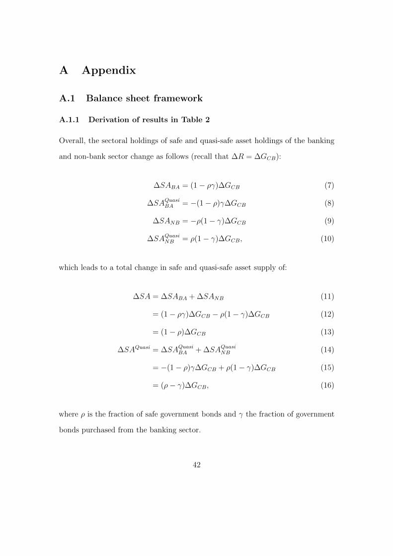
A.1.1 Derivation of results in Table 2

Overall, the sectoral holdings of safe and quasi-safe asset holdings of the banking

and non-bank sector change as follows (recall that ∆R = ∆GCB):

∆SABA = (1− ργ)∆GCB (7)

∆SAQuasiBA = −(1− ρ)γ∆GCB (8)

∆SANB = −ρ(1− γ)∆GCB (9)

∆SAQuasiNB = ρ(1− γ)∆GCB, (10)

which leads to a total change in safe and quasi-safe asset supply of:

∆SA = ∆SABA + ∆SANB (11)

= (1− ργ)∆GCB − ρ(1− γ)∆GCB (12)

= (1− ρ)∆GCB (13)

∆SAQuasi = ∆SAQuasiBA + ∆SAQuasi

NB (14)

= −(1− ρ)γ∆GCB + ρ(1− γ)∆GCB (15)

= (ρ− γ)∆GCB, (16)

where ρ is the fraction of safe government bonds and γ the fraction of government

bonds purchased from the banking sector.

42

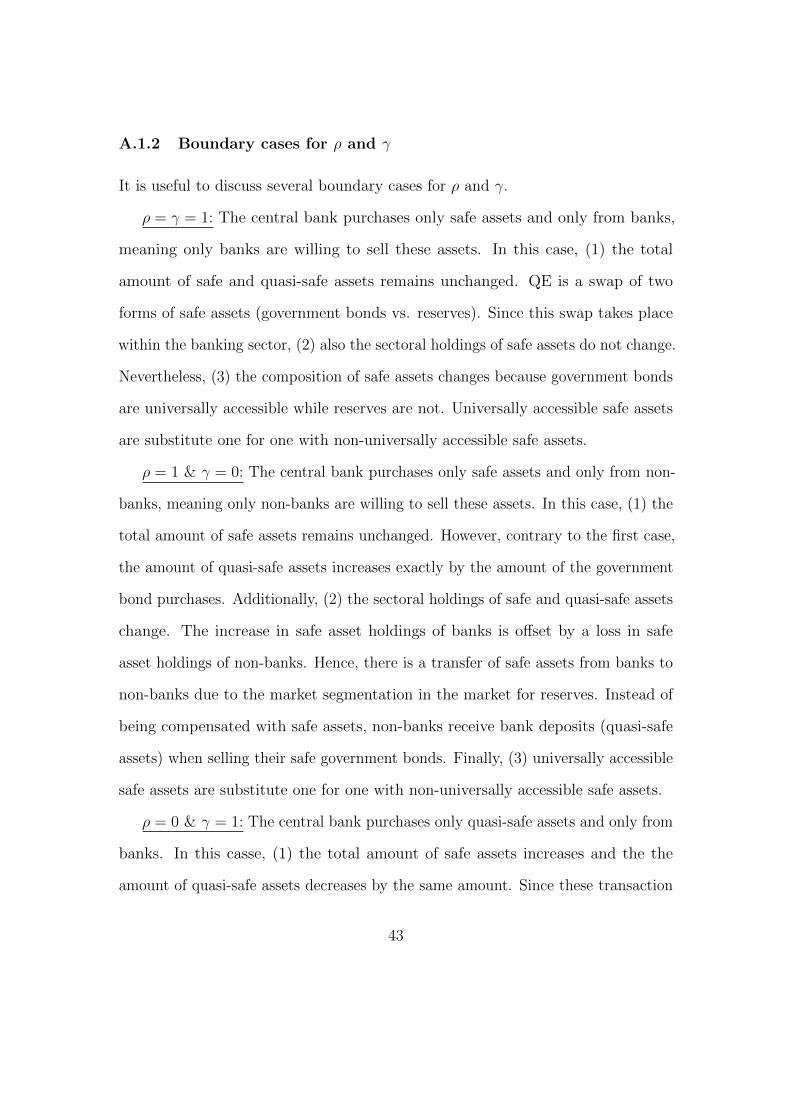
A.1.2 Boundary cases for ρ and γ

It is useful to discuss several boundary cases for ρ and γ.

ρ = γ = 1: The central bank purchases only safe assets and only from banks,

meaning only banks are willing to sell these assets. In this case, (1) the total

amount of safe and quasi-safe assets remains unchanged. QE is a swap of two

forms of safe assets (government bonds vs. reserves). Since this swap takes place

within the banking sector, (2) also the sectoral holdings of safe assets do not change.

Nevertheless, (3) the composition of safe assets changes because government bonds

are universally accessible while reserves are not. Universally accessible safe assets

are substitute one for one with non-universally accessible safe assets.

ρ = 1 & γ = 0: The central bank purchases only safe assets and only from non-

banks, meaning only non-banks are willing to sell these assets. In this case, (1) the

total amount of safe assets remains unchanged. However, contrary to the first case,

the amount of quasi-safe assets increases exactly by the amount of the government

bond purchases. Additionally, (2) the sectoral holdings of safe and quasi-safe assets

change. The increase in safe asset holdings of banks is offset by a loss in safe

asset holdings of non-banks. Hence, there is a transfer of safe assets from banks to

non-banks due to the market segmentation in the market for reserves. Instead of

being compensated with safe assets, non-banks receive bank deposits (quasi-safe

assets) when selling their safe government bonds. Finally, (3) universally accessible

safe assets are substitute one for one with non-universally accessible safe assets.

ρ = 0 & γ = 1: The central bank purchases only quasi-safe assets and only from

banks. In this casse, (1) the total amount of safe assets increases and the the

amount of quasi-safe assets decreases by the same amount. Since these transaction

43

take place on the balance sheet of the banking sector, (2) the (quasi-)safe asset

holdings of non-banks remain unchanged. (3) The amount of universally accessible

safe assets remains unchanged because the central bank purchases only quasi-

safe assets. Simultaneously, the amount of non-universally accessible safe assets

increases because the central bank pays its purchases with newly creates reserves.

ρ = 0 & γ = 0: The central bank purchases only quasi-safe assets and only from

non-banks. In this case, (1) the total amount of safe assets increases and the

amount of quasi-safe assets remains unchanged. The former is due to the fact

that banks receive safe reserves because they act as intermediary. Hence, (2) the

safe asset holdings of the banking sector increase. The latter is due to the fact

that non-banks are compensated with bank deposits. They swap two forms of

quasi-safe assets such that their (quasi-)safe asset holdings remain unchanged.

(3) The amount of universally accessible safe assets remains unchanged because

the central bank purchases only quasi-safe assets. Simultaneously, the amount of

non-universally accessible safe assets increases because the central bank pays its

purchases with newly creates reserves.

A.2 Balance sheet framework extension: positive net is-

suance of new government bonds

The net issuance of government bonds is an important driver of changes in total

and sectoral holdings of government bonds. Against this background, we extend our

framework. We assume that an exogenous treasury can change the net debt level

by purchasing or selling government bonds.18 Contrary to central bank purchases,

18Note, that selling (purchasing) government bonds corresponds to the situation in which theamount of newly issued government bonds exceeds (is smaller than) the amount of maturing ones,

44

these operations change the amount of outstanding government bonds, i.e., ∆G 6= 0.

Since governments usually increase their net debt levels, we consider the case in

which the treasury sells bonds, i.e., ∆G > 0. We assume it sells a fraction κ to

the banking and (1− κ) to the non-bank sector. Additionally, we introduce the

parameters [ρ1, ρ2] to distinguish between safe and quasi-safe government bonds;

ρ1 represent the amount of safe assets purchased by the central bank as a share of

total purchases and ρ2 represents the amount of safe assets issued by the treasury

as a share of total net issuance.

Table 6 presents the change in total and sectoral holdings of (quasi-)safe assets,

if we allow for changes in government debt levels. Derivations can be found in

the Appendix. Since the banking sector acts as an intermediary for non-banks, it

receives additional reserves whenever banks or non-banks sell government bonds

to the central bank. Hence, reserve holdings increase by ∆GCB. Similarly, the

banking sector spends reserves whenever banks or non-banks purchase newly issued

government bonds. Hence, the reserve holdings decrease by ∆G. To arrive at the

total change in safe asset holdings of the banking sector, we still need to take into

account that banks sell safe government bonds to the central bank. This reduces

their safe asset holdings by ρ1γ. Additionally, they purchase safe newly issued

government bonds. This increases their safe asset holdings by ρ2κ∆G. Taken

together, the total change in safe asset holdings of the banking sector amounts to

(1− ρ1γ)∆GCB − (1− ρ2κ)∆G.

The banking sector reduces its quasi-safe asset holdings by (1 − ρ1)γ∆GCB

because it sells quasi-safe government bonds to the central bank. Simultaneously,

it increases its quasi-safe asset holdings by (1 − ρ2)κ∆G because it purchases

such that the net indebtedness of the government increases (decreases).

45

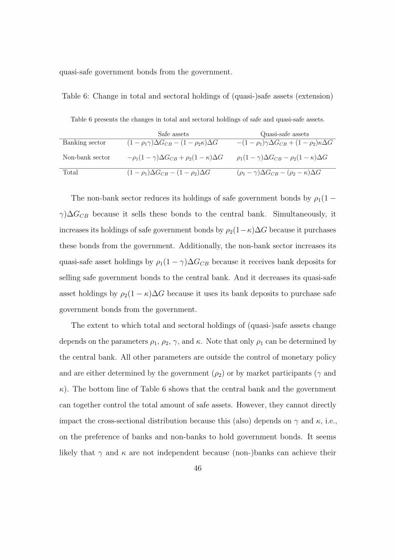
quasi-safe government bonds from the government.

Table 6: Change in total and sectoral holdings of (quasi-)safe assets (extension)

Table 6 presents the changes in total and sectoral holdings of safe and quasi-safe assets.

Safe assets Quasi-safe assetsBanking sector (1− ρ1γ)∆GCB − (1− ρ2κ)∆G −(1− ρ1)γ∆GCB + (1− ρ2)κ∆G

Non-bank sector −ρ1(1− γ)∆GCB + ρ2(1− κ)∆G ρ1(1− γ)∆GCB − ρ2(1− κ)∆G

Total (1− ρ1)∆GCB − (1− ρ2)∆G (ρ1 − γ)∆GCB − (ρ2 − κ)∆G

The non-bank sector reduces its holdings of safe government bonds by ρ1(1−

γ)∆GCB because it sells these bonds to the central bank. Simultaneously, it

increases its holdings of safe government bonds by ρ2(1−κ)∆G because it purchases

these bonds from the government. Additionally, the non-bank sector increases its

quasi-safe asset holdings by ρ1(1− γ)∆GCB because it receives bank deposits for

selling safe government bonds to the central bank. And it decreases its quasi-safe

asset holdings by ρ2(1− κ)∆G because it uses its bank deposits to purchase safe

government bonds from the government.

The extent to which total and sectoral holdings of (quasi-)safe assets change

depends on the parameters ρ1, ρ2, γ, and κ. Note that only ρ1 can be determined by

the central bank. All other parameters are outside the control of monetary policy

and are either determined by the government (ρ2) or by market participants (γ and

κ). The bottom line of Table 6 shows that the central bank and the government

can together control the total amount of safe assets. However, they cannot directly

impact the cross-sectional distribution because this (also) depends on γ and κ, i.e.,

on the preference of banks and non-banks to hold government bonds. It seems

likely that γ and κ are not independent because (non-)banks can achieve their

46

preferred level of safe asset holdings by adjusting the amount of government bonds

they sell to the central bank (γ) and/or the amount they purchase in primary

auctions (κ).

Against this background, we derive a measure for the preference to hold safe

government bonds as a function of γ and κ, which we can later bring to the data.

To this end, we define define γ = γBank and (1− γ) = γNon−bank = γICPF + γOFI +

γHH + γOther + γForeign. We do the same for κ. Using SHSSdata, we are able to

measure the change in safe government bond holdings of our sectors ∆Gssafe, where

s ∈ {Bank, ICPF,OFI,HH,Other, Foreign}. Against this background, we use

∆Gssafe

Gssafe

= −(ρ1γs∆GCB + ρ2κ

s∆G)

Gssafe

(17)

as a measure for the cross-sectional variation in the preference to hold safe govern-

ment bonds. We can do this because the only driver of cross-sectional variation in

this measure is variation in γ and κ.

Finally, we can use the results presented in Table 6 to derive conditions for the

neutrality of QE when allowing the total amount of outstanding government bonds

G to change. As in Proposition 1, we can derive these conditions for (1) the total

amount, (2) the sectoral holdings, and (3) the composition of safe assets.

Proposition 2 (Safe asset neutrality of QE)

(i) QE is neutral to the total amount of safe assets if

• ρ1 = ρ2 = 1, i.e., if the central bank purchases only safe government

bonds and only safe government bonds are issued

• ρ1∆GCB = ρ2∆G, i.e., the amount of safe government bonds purchased

47

by the central bank equals the amount of newly issued safe government

bonds

(ii) QE is neutral to the sectoral holdings of safe assets if

• ρ1 = ρ2 = γ = κ = 1, i.e., if the central bank purchases only safe

government bonds and only from banks; and if only safe government

bonds are issued and only to banks

• ∆GCB = ∆G & ρ1 = ρ2 & γ = κ, i.e., the amount of government

bonds purchased by the central bank equals the amount of newly issued

government bonds, the share of safe government bonds purchased by

the central bank equals the share of safe government bonds in primary

auctions, and the share of bonds purchased from banks equals the share

issued to banks

(iii) QE is never neutral to the composition of safe assets, i.e., to the share of

universally accessible and non-accessible safe asset.

A.3 Data characteristics

The SHSS data vintage used for our sample refers to June 2020 and data is collected

on a quarterly basis by euro-area custodians. Sectors in the SHSS database are

defined according to the ESA 2010 classification. Securities held exclusively by

non-euro area sectors that are not held via a euro area custodians are not available

in SHSS and, thereafter, neither their amount outstanding. In addition, securities

which have not been redeemed yet, but have a negative residual maturity can still

be reported in the investors holdings portfolio. Thus we do not include securities

48

with negative residual maturity according to CSDB. We define government bonds

as securities issued by ESA 2010 sectors S 13, S 1311, S 1312, S 1313 and S 1314

(general, central and local government and social security), and agency bonds

(i.e. corporate bonds backed by the government) and supras held under PSPP.

The classifications of the CSDB debt type variable changes after 2016Q3. Up to

2016Q3, we define corporate bonds as debt types D.1, D.11, D.15, D.16, D.164,

D.18, D.3 and D.32 and which are not issued by the government sector, as well

as securities included in the ECB’s Corporate sector purchase program. Covered

bonds and asset-back securities correspond to debt types D.21, D.23 and D.233

which are not issued by the government sector, as well as to securities included in

the ECB’s asset-backed securities purchase program and covered bond purchase

program 3. After 2016Q3, we still follow the securities classification according to the

inclusion into the corresponding ECB’s purchase programs, but we define corporate

bonds as debt types D.1, D.11, D.14, D.141, D.15, D.16, D.18, D. 181, D.1811,

D.1812, D.1813, D.1819, D.182, D.1821 and D.1822 and which are not issued by

the government sector; and covered bonds and asset-back securities correspond to

debt types D.13, D.131 and D.139 and not issued by the government sector.

49