quantitative thermo-acoustics and related problems · quantitative thermo-acoustics and related...

Quantitative Thermo-acoustics and related problems

Guillaume Bal

Department of Applied Physics & Applied Mathematics, Columbia University, New

York, NY 10027

E-mail: [email protected]

Kui Ren

Department of Mathematics, University of Texas at Austin, Austin, TX 78712


Gunther Uhlmann

Department of Mathematics, UC Irvine, Irvine, CA 92697 and Department of

Mathematics, University of Washington, Seattle, WA 98195


Ting Zhou

Department of Mathematics, University of Washington, Seattle, WA 98195


Abstract. Thermo-acoustic tomography is a hybrid medical imaging modality that

aims to combine the good optical contrast observed in tissues with the good resolution

properties of ultrasound. Thermo-acoustic imaging may be decomposed into two steps.

The first step aims at reconstructing an amount of electromagnetic radiation absorbed

by tissues from boundary measurements of ultrasound generated by the heating caused

by these radiations. We assume this first step done. Quantitative thermo-acoustics

then consists of reconstructing the conductivity coefficient in the equation modeling

radiation from the now known absorbed radiation. This second step is the problem of

interest in this paper.

Mathematically, quantitative thermo-acoustics consists of reconstructing the

conductivity in Maxwell’s equations from available internal data that are linear in the

conductivity and quadratic in the electric field. We consider several inverse problems

of this type with applications in thermo-acoustics as well as in acousto-optics. In this

framework, we obtain uniqueness and stability results under a smallness constraint on

the conductivity. This smallness constraint is removed in the specific case of a scalar

model for electromagnetic wave propagation for appropriate illuminations constructed

by the method of complex geometric optics (CGO) solutions.

Keywords. Photo-acoustics, Thermo-acoustics, inverse scattering with internal data,

inverse problems, acousto-optics stability estimates, complex geometrical optics (CGO)

solutions.

Quantitative Thermo-acoustics and related problems 2

1. Introduction

Thermo-acoustic tomography and photo-acoustic tomography are based on what we

will refer to as the photo-acoustic effect: a fraction of propagating radiation is absorbed

by the underlying medium. This results in local heating and hence local mechanical

expansion of the medium. This in turn generates acoustic pulses that propagate to the

domain’s boundary. The acoustic signal is measured at the domain’s boundary and

used to reconstruct the amount of absorbed radiation. The reconstruction of absorbed

radiation is the first step in both thermo-acoustic and photo-acoustic tomography.

What distinguishes the two modalities is that in photo-acoustic tomography (also called

acousto-optic tomography), radiation is high-frequency radiation (near-infra-red with

sub-µm wavelength) while in thermo-acoustics, radiation is low-frequency radiation

(microwave with wavelengths comparable to 1m).

The second step in photo- and thermo-acoustic tomography is called quantitative

photo- or thermo-acoustics and consists of reconstructing the absorption coefficient from

knowledge of the amount of absorbed radiation. This second step is different in thermo-

acoustic and photo-acoustics as radiation is typically modeled by Maxwell’s equations

in the former case and transport or diffusion equations in the latter case. The problem

of interest in the paper is quantitative thermo-acoustics.

For physical descriptions of the photo-acoustic effect, which we could also call the

thermo-acoustic effect, we refer the reader to the works [6, 7, 8, 12, 26, 27] and their

references. For the mathematical aspects of the first step in thermo- and photo-acoustics,

namely the reconstruction of the absorbed radiation map from boundary acoustic wave

measurements, we refer the reader to e.g. [1, 10, 11, 13, 14, 15, 18, 20, 23]. Serious

difficulties may need to be addressed in this first step, such as e.g. limited data, spatially

varying acoustic sound speed [1, 15, 23], and the effects of acoustic wave attenuation

[17]. In this paper, we assume that the absorbed radiation map has been reconstructed

satisfactorily.

In thermo-acoustics, where radiation is modeled by an electromagnetic field E(x)

solving (time-harmonic) Maxwell’s equations, absorbed radiation is described by the

product H(x) = σ(x)|E(x)|2. The second step in the inversion thus concerns the

reconstruction of σ(x) from knowledge of H(x). This paper presents several uniqueness

and stability results showing that in several settings, the reconstruction of σ(x) from

knowledge of H(x) is a well-posed problem. These good stability properties were

observed numerically in e.g., [19], where it is also stated that imaging H(x) may not

provide a faithful image for σ(x) because of diffraction effects.

In photo-acoustics, radiation is modeled by a radiative transfer equation or a

diffusion equation. Several results of uniqueness in the reconstruction of the absorption

and scattering coefficients have been obtain recently. We refer the reader to e.g.,

[5, 7, 8, 22], for works on quantitative photoacoustics in the mathematics and

bioengineering literatures.

After recalling the equations modeling radiation propagation and acoustic


propagation, we define in section 2 below the mathematical problems associated to

quantitative thermo-acoustics. We mainly consider two problems: a system of time-

harmonic Maxwell equations and a scalar approximation taking the form of a Helmholtz

equation.

This paper presents two different results. The first result, presented in section

3, is a uniqueness and stability result under the condition that σ is sufficiently small

(as a bounded function). This result, based on standard energy estimates, works for

general problems of the form Hu = σu and includes the thermo-acoustic models both

in the vectorial and scalar cases. The same technique also allows us to reconstruct

σ when H = ∆ the Laplace operator. This has applications in simplified models of

acousto-optics as they arise, e.g., in [4].

The second result removes the smallness constraint on σ for the (scalar) Helmholtz

model of radiation propagation. The result is based on proving convergence of a fixed

point iteration for the conductivity σ under the assumption that σ is sufficiently regular

and that the electromagnetic illumination applied to the boundary of the domain is

well-chosen. In some sense, the smallness constraint on σ is traded against a constraint

on the type of electromagnetic illumination that is applied. The method of proof is

based on using complex geometric optics (CGO) solutions that are asymptotically, as

a parameter ρ → ∞, independent of the unknown term σ. Such CGO’s allow us to

construct a contracting functional on σ provided that the electromagnetic illumination

is well-chosen (in a non-explicit way). The technique of CGO solutions is similar to

their use in quantitative reconstructions in photo-acoustics as they were presented in

[5].

2. Quantitative thermo-acoustics

2.1. Modeling of the electromagnetic radiation

The propagation of electromagnetic radiation is given by the equation for the electric

field1

c2

∂2

∂t2E + σµ

∂

∂tE +∇×∇× E = S(t, x), (1)

for t ∈ R and x ∈ R3. Here, c2 = (εµ)−1 is the light speed in the domain of interest, ε the

permittivity, µ the permeability, and σ = σ(x) the conductivity we wish to reconstruct.

Let us consider the scalar approximation to the above problem:

1

c2

∂2

∂t2u+ σµ

∂

∂tu−∆u = S(t, x), (2)

for t ∈ R and x ∈ Rn for n ≥ 2 an arbitrary dimension. This approximation will be

used to simplify some derivations in the paper. One of the main theoretical results in

the paper (presented in section 4) is at present obtained only for the simplified scalar

setting.

Let ωc = ck be a given frequency, which we assume corresponds to a wavelength

λ = 2πk

that is comparable or large compared to the domain we wish to image. We


assume that S(t, x) is a narrow-band pulse with central frequency ωc of the form

−e−iωctφ(t)S(x), where φ(t) is the envelope of the pulse and S(x) is a superposition

of plane waves with wavenumber k such that ωc = ck. As a consequence, upon taking

the Fourier transform in the above equation and assuming that all frequencies satisfy a

similar equation, we obtain that

u(t, x) ∼ φ(t)u(x),

where

∆u+ k2u+ ikcµσu = S(x). (3)

We recast the above equation as a scattering problem with incoming radiation ui(x)

and scattered radiation us(x) satisfying the proper Sommerfeld radiation conditions

at infinity. Replacing cµσ by σ to simplify notation, we thus obtain the model for

electromagnetic propagation:

∆u+ k2u+ ikσ(x)u = 0, u = ui + us. (4)

The incoming radiation ui is a superposition of plane waves of the form ui = eikξ·x with

ξ ∈ S2 and is assumed to be controlled experimentally.

2.2. Modeling of the acoustic radiation

The amount of absorbed radiation by the underlying medium as the electromagnetic

waves propagate is given by

H(t, x) = σ(x)|u(t, x)|2 ∼ φ2(t)σ(x)|u|2(x). (5)

A thermal expansion (assumed to be proportional to H) results and acoustic waves are

emitted. Such waves are modeled by

1

c2s(x)

∂2p

∂t2−∆p = β

∂

∂tH(t, x), (6)

with cs the sound speed and β a coupling coefficient measuring the strength of the

photoacoustic effect. We assume β to be constant and known. The pressure p(t, x) is

then measured on ∂X as a function of time.

The first task in thermo-acoustics is to solve an inverse wave problem consisting of

reconstructing H(t, x) from knowledge of p(t, x) measured on ∂X as a function of time.

The latter problem is however extremely underdetermined when H(t, x) is an arbitrary

function of time and space. In order for the inverse wave problem to be well-posed,

restrictions on H(t, x) need to be performed. Typically, a separation of time scales is

invoked to ensure that H(t, x) has a support in time that is small compared to the time

scale of acoustic wave propagation. When such a separation of scale is valid, we obtain

as in [2] that

H(t, x) = H(x)δ0(t), H(x) = σ(x)

∫R|u(t, x)|2dt = σ(x)|u(x)|2

∫Rφ2(t)dt. (7)


We assume that the pulse intensity is normalized so that∫R φ

2(t)dt = 1. The above

separation of scales holds for measurements of acoustic frequencies that are comparable

to or smaller than the frequency of the pulse φ(t). Typical experiments are performed

for pulses of duration τ := 0.5µs. For a sound speed of cs = 1.5 103m/s, this corresponds

to a spatial scale of 0.75mm. In other words, the approximation (7) is valid for time

scales larger than 0.5µs, which corresponds to a physical resolution (typically chosen to

be 12λ) limited by λ = 0.75mm.

Real measurements correspond to sources of the form φ2(t) ∗H(x)δ0(t), which are

therefore convolved at the time scale τ . This corresponds in the reconstruction of H(x)

to a blurring at the scale λ. As a consequence, details of H(x) at the scale below 12λ

cannot be reconstructed in a stable manner.

At any rate, we assume the first step in thermoacoustic tomography, namely the

reconstruction of H(x) from knowledge of pressure p(t, x) on ∂X done. It then remains

to reconstruct σ from knowledge of H.

2.3. Inverse Scattering Problems with Internal Data

We are now ready to present the inverse problems with internal data we consider in this

paper. We recall that u is modeled as the solution to (4). The incoming condition is

imposed experimentally. We assume here that we can construct prescribed illuminations

ui given as arbitrary superposition of plane waves eikξ·x with ξ ∈ S2.

Traces u|∂X of solutions to (4) are dense in H12 (∂X) [16]. As a consequence, for

each g ∈ H 12 (∂X), we can find a sequence of illuminations ui such that the solution u

in the limit is the solution of

∆u+ k2u+ ikσ(x)u = 0, X

u = g ∂X,(8)

for a given boundary condition g(x). The internal data are then of the form

H(x) = σ(x)|u|2(x). (9)

It remains to find procedures that allow us to uniquely reconstruct σ(x) from knowledge

of H(x) with a given illumination. We shall consider two different theories. The first one

assumes a specific form of g but allows us to reconstruct arbitrary (sufficiently smooth)

σ while the second one applies for general illuminations g but only for small (though

not necessarily smooth) functions σ(x).

The above derivation can be generalized to the full system of Maxwell’s equations.

We then obtain the following inverse problem. Radiation is modeled by

−∇×∇× E + k2E + ikσ(x)E = 0, X

ν × E = g ∂X.(10)

In the vectorial case, the internal data, i.e., the amount of absorbed electromagnetic

radiation, are then of the form

H(x) = σ(x)|E|2(x). (11)


3. A general class of inverse problems with internal data

The above problems are examples of a more general class we define as follows. Let

P (x,D) be an operator acting on functions defined in Cm for m ∈ N∗ an integer and

with values in the same space and let B be a linear boundary operator defined in the

same spaces. Consider the equation

P (x,D)u = σ(x)u, x ∈ XBu = g, x ∈ ∂X.

(12)

We assume that the above equation admits a unique weak solution in some Hilbert space

H1 for sufficiently smooth illuminations g(x) on ∂X.

For instance, P could be the Helmholtz operator ik−1(∆+k2) seen in the preceding

section with u ∈ H1 := H1(X;C) and g ∈ H12 (∂X;C) with B the trace operator on

∂X. Time -harmonic Maxwell’s equations can be put in that framework with m = n

and

P (x,D) =1

ik(∇×∇×−k2). (13)

We impose an additional constraint on P (x,D) that the equation P (x,D)u = f on

X with Bu = 0 on ∂X admits a unique solution in H = L2(X;Cm). For instance,

H = L2(X;C) in the example seen in the preceding section in the scalar approximation

provided that k2 is not an eigenvalue of −∆ on X. For Maxwell’s equations, the above

constraint is satisfied so long as k2 is not an internal eigenvalue of the Maxwell operator

[9]. This is expressed by the existence of a constant α > 0 such that:

(P (x,D)u, u)H ≥ α(u, u)H. (14)

Finally we assume that the conductivity σ is bounded from above by a positive

constant:

0 < σ(x) ≤ σM(x) a.e. x ∈ X. (15)

We denote by ΣM the space of functions σ(x) such that (15) holds. Measurements are

then of the form H(x) = σ(x)|u|2, where | · | is the Euclidean norm on Cm. Then we

have the following result.

Theorem 3.1 Let σj ∈ ΣM for j = 1, 2. Let uj be the solution to P (x,D)uj = σjuj in

X with Buj = g on ∂X for j = 1, 2. Define the internal data Hj(x) = σj(x)|uj(x)|2 on

X.

Then for σM sufficiently small so that σM < α, we find that:

(i) [Uniqueness] If H1 = H2 a.e. in X, then σ1(x) = σ2(x) a.e. in X where H1 = H2 > 0.

(ii) [Stability] Moreover, we have the following stability estimate

‖w1(√σ1 −

√σ2)‖H ≤ C‖w2(

√H1 −

√H2)‖H, (16)

for some universal constant C and for positive weights given by

w21(x) =

∏j=1,2

|uj|√σj

(x), w2(x) =1

α− supx∈X

√σ1σ2

maxj=1,2

√σj|uj′|

(x) + maxj=1,2

1√σj

(x). (17)


Here j′(j) = (2, 1) for j = (1, 2).

The weights w1 and w2 are written here in terms of the conductivities σj and the

radiation solutions uj. Under appropriate conditions on the solution uj, these weights

can be bounded above and below by explicit constants. In such circumstances, the above

theorem thus shows that the reconstruction of σ is Lipschitz-stable in H with respect

to errors in the available data H.

Proof. Some straightforward algebra shows that

P (x,D)(u1 − u2) =√σ1σ2

(|u2|u1 − |u1|u2

)+ (√H1 −

√H2)

(√σ1

|u1|−√σ2

|u2|

).

Here we have defined u = u|u| . Although this does not constitute an equation for u1−u2,

it turns out that

||u2|u1 − |u1|u2| = |u2 − u1|,

as can easily be verified. Our assumptions on P (x,D) then imply that

(α− supx∈X

√σ1σ2)‖u1 − u2‖2

H ≤(

(√H1 −

√H2)

(√σ1

|u1|−√σ2

|u2|

), u1 − u2

)H,

and a corresponding bound for u1 − u2:

(α− supx∈X

√σ1σ2)‖u1 − u2‖H ≤

∥∥∥(√H1 −

√H2)

(√σ1

|u1|−√σ2

|u2|

)∥∥∥H.

Now, we find that

|u1| − |u2| =√H1√σ1

−√H2√σ2

= (H1H2)14

( 1√σ1

− 1√σ2

)+ (H

141 −H

142 )( H 1

41√σ1

− H142√σ2

).

Using (H141 −H

142 )(H

141 +H

142 ) = (H

121 −H

122 ) and ||u1| − |u2|| ≤ |u1− u2|, we obtain (16).

Reconstructions for a simplified acousto-optics problem. In thermo-acoustics, the

operator P (x,D) considered in the preceding section is purely imaginary as can be

seen in (13). In a simplified version of the acousto-optics problem considered in [4], it

is interesting to look at the problem where P (x,D) = ∆ and where the measurements

are given by H(x) = σ(x)u2(x). Here, u is thus the solution of the elliptic equation

(−∆ + σ)u = 0 on X with u = g on ∂X. Assuming that g is non-negative, which is the

physically interesting case, we obtain that |u| = u and hence

∆(u1 − u2) =√σ1σ2(u2 − u1) + (

√H1 −

√H2)

( σ1√H1

− σ2√H2

).

Therefore, as soon as 0 is not an eigenvalue of ∆ +√σ1σ2, we obtain that u1 = u2 and

hence that σ1 = σ2. In this situation, we do not need the constraint that σ is small.

For instance, for σ0 such that 0 is not an eigenvalue of ∆ + σ0, we find that for σ1


and σ2 sufficiently close to σ0, then H1 = H2 implies that σ1 = σ2 on the support of

H1 = H2. This particular situation, where a spectral equation arises for u2 − u1, seems

to be specific to the problem with P (x,D) = ∆ and u is a non-negative scalar quantity.

Similarly, when P (x,D) = −∆, it was proved recently in [25] that the measurements

uniquely and stably determine σ in the Helmholtz equation (∆ + σ)u = 0.

However, it is shown in [3] that two different, positive, absorptions σj for j = 1, 2,

may in some cases provide the same measurement H = σju2j with ∆uj = σjuj on

X with uj = g on ∂X and in fact σ1 = σ2 on ∂X so that these absorptions cannot be

distinguished by their traces on ∂X. Such a result should be compared to non-uniqueness

results in the theory of semi-linear partial differential equations. This counter-example

shows, that the smallness condition in Theorem 3.1 is necessary in general.

In the setting of thermo-acoustics, the theorem above is valid also only when the

σ is sufficiently small. In the scalar case of thermo-acoustics, however, the smallness

condition can be removed under additional assumptions on the illumination g.

4. The scalar Helmholtz equation.

Such illuminations are constructed using Complex Geometrical Optics (CGO) solutions

as in the inverse problem considered in [5], although the method of proof is somewhat

different in the thermo-acoustic context. Our proof here is based on showing that an

appropriate functional of σ admits a unique fixed point. This can be done when the

conductivity σ is sufficiently smooth. We assume that σ ∈ Hp(X) for p > n2

and

construct

q(x) = k2 + ikσ(x) ∈ Hp(X), p >n

2. (18)

Moreover, q(x) is the restriction to X of the compactly supported function (still called

q) q ∈ Hp(Rn). The extension is chosen so that [24, Chapter VI, Theorem 5]

‖q|X‖Hp(X) ≤ C‖q‖Hp(Rn), (19)

for some constant C independent of q.

Then (8) is recast as

∆u+ q(x)u = 0, X

u = g ∂X.(20)

We recall that measurements are of the form H(x) = σ(x)|u|2(x).

We construct g as the trace of the CGO solution of

∆u+ qu = 0, Rn, (21)

with u = eρ·x(1 + ψρ) with

ρ · ρ = 0 (22)


and ψρ solution in L2δ (see (25) below) of the equation:

∆ψρ + 2ρ · ∇ψρ = −q(x)(1 + ψρ), Rn. (23)

The data then take the form

e−(ρ+ρ)·xH(x) = σ(x) +H[σ](x), H[σ](x) = σ(x)(ψρ + ψρ + ψρψρ). (24)

It remains to show that H[σ](x) is a contraction, which is a sufficient condition for (24)

to admit a unique solution. We do this in the space Y = Hn2

+ε(X) where n is spatial

dimension. This is an algebra and we know that if σ is in that space, then the restriction

of ψρ to X is also in that space. Moreover ρψρ is bounded in that norm independently

of ρ. The contraction property of H for ρ sufficiently large stems from the contraction

property of σ → ψρ[σ] for ρ sufficiently large. For the latter, we need to adapt the

results proved in [5] to obtain Lipschitzness of ψρ with respect to σ in the space Y with

its natural norm.

The Lipschitzness is obtained as follows. We introduce the spaces Hsδ for s ≥ 0 as

the completion of C∞0 (Rn) with respect to the norm ‖ · ‖Hsδ

defined as

‖u‖Hsδ

=(∫

Rn〈x〉2δ|(I −∆)

s2u|2dx

) 12, 〈x〉 = (1 + |x|2)

12 . (25)

Here (I−∆)s2u is defined as the inverse Fourier transform of 〈ξ〉su(ξ), where u(ξ) is the

Fourier transform of u(x).

We define Y = Hp(X) and M as the space of functions in Y with norm bounded

by a fixed M > 0.

Lemma 4.1 Let ψ be the solution of

∆ψ + 2ρ · ∇ψ = −q(1 + ψ), (26)

and ψ be the solution of the same equation with q replaced by q, where q is defined as in

(18) with σ replaced by σ. We assume that q and q are in M. Then there is a constant

C such that for all ρ with |ρ| ≥ |ρ0|, we have

‖ψ − ψ‖Y ≤C

|ρ|‖σ − σ‖Y . (27)

Proof. We proceed as in [5] and write

ψ =∑j≥0

ψj,

with

(∆ + 2ρ · ∇)ψj = −qψj−1, j ≥ 0 (28)

with ψ−1 = 1. This implies that

(∆ + 2ρ · ∇)(ψj − ψj) = −((q − q)ψj−1 + q(ψj−1 − ψj−1)

). (29)


In the proof of [5, Proposition 3.1], it is shown that for some constant C independent

of ρ for |ρ| sufficiently large,

‖ψj‖Hsδ≤ C|ρ|−1‖q‖Hs

1‖ψj−1‖Hs

δ,

where by a slight abuse of notation, ‖ψ−1‖Hsδ≡ 1. We assume that C|ρ|−1‖q‖Hs

1< 1 for

|ρ| sufficiently large so that the above series is summable in j. Let us still denote by ψjthe restriction of ψj to X. Since 〈x〉 is bounded on X, we deduce from (19) that

‖ψj‖Y ≤ C|ρ|−1‖q‖Y ‖ψj−1‖Y . (30)

Upon defining εj = ‖ψj−ψj‖Y , we deduce from (30) and (29) that for some constant

C,

|ρ|εj ≤ C‖ψj−1‖Y ‖q − q‖Y + CMεj−1,

with ε−1 = 0. Summing over 0 ≤ j ≤ J yields

J∑j=0

εj ≤C

|ρ|‖q − q‖Y

J∑j=0

‖ψj−1‖Y +CM

|ρ|

J−1∑j=0

εj.

When ρ is sufficiently large so that r := CM |ρ|−1 < 1, we obtain that∑j≥0

εj ≤C‖q − q‖Y(1− r)|ρ|

∑j≥0

‖ψj−1‖Y ≤C ′

(1− r)|ρ|(1 + ‖q‖Y )‖q − q‖Y .

This shows that

‖ψ − ψ‖Y ≤∑j≥0

‖ψ − ψ‖Y ≤C

|ρ|‖q − q‖Y ≤

Ck

|ρ|‖σ − σ‖Y . (31)

This concludes the proof of the lemma.

From this, we obtain the

Corollary 4.2 Let |ρ| ≥ ρ0 for ρ0 sufficiently large. Then there exists a constant r < 1

such that

‖H[σ]−H[σ]‖Y ≤ r‖σ − σ‖Y . (32)

Proof. We recall that

H[σ](x) = σ(x)(ψρ + ψρ + ψρψρ).

Since Y is an algebra and σ and ψρ are bounded in Y , we deduce from the preceding

lemma the existence of a constant C such that

‖H[σ]−H[σ]‖Y ≤C

|ρ|‖σ − σ‖Y .

It remains to choose |ρ| sufficiently large to show that H is a contraction from Y to Y .

We thus deduce the reconstruction algorithm

σ = limm→∞

σm, σ0 = 0, σm(x) = e−(ρ+ρ)·xH(x)−H[σm−1](x), m ≥ 1.


4.1. Reconstructions for the inverse scattering problem

The above method allows us to uniquely reconstruct σ provided that gρ := uρ|∂X is

chosen as a boundary illumination. Let now g be close to gρ and define

(∆ + q)u = 0, X, u = g ∂X.

We also define uρ the CGO calculated with q with trace gρ on ∂X as well as u solution

of

(∆ + q)u = 0, X, u = g ∂X.

Then we find that

(∆ + q)(u− uρ) = 0 X, u− uρ = g − gρ ∂X,

as well as

(∆ + q)(u− uρ) = 0 X, u− uρ = g − gρ ∂X.

Let us define Z = Hp− 12 (∂X). We can show the following result:

Theorem 4.3 Let ρ ∈ Cn be such that |ρ| is sufficiently large and ρ · ρ = 0. Let σ and

σ be functions in M.

Let g ∈ Z be a given illumination and H(x) be the measurement given in (9) for

u solution of (8). Let H(x) be the measurement constructed by replacing σ by σ in (9)

and (8).

Then there is an open set of illuminations g in Z such that H(x) = H(x) in Y

implies that σ(x) = σ(x) in Y . Moreover, there exists a constant C independent of σ

and σ in M such that

‖σ − σ‖Y ≤ C‖H − H‖Y . (33)

More precisely, we can write the reconstruction of σ as finding the unique fixed point

to the equation

σ(x) = e−(ρ+ρ)·xH(x)−Hg[σ](x), in Y. (34)

The functional Hg[σ] defined as

Hg[σ](x) = σ(x)(ψg(x) + ψg(x) + ψg(x)ψg(x)), (35)

is a contraction map for g in the open set described above, where ψg is defined as the

solution to

(∆ + 2ρ · ∇)ψg = −q(1 + ψg), X, ψg = e−ρ·xg − 1 ∂X. (36)

We thus deduce the reconstruction algorithm

σ = limm→∞

σm, σ0 = 0, σm(x) = e−(ρ+ρ)·xH(x)−Hg[σm−1](x), m ≥ 1. (37)


Proof. We deduce from Lemma 4.1 and standard trace theorems that

‖ψ|∂X − ψ|∂X‖Z ≤C

|ρ|‖σ − σ‖Y .

Let g0 = eρ·x(1 + ψ|∂X) so that ψg0 = ψ. We have, using Lemma 4.1 again and elliptic

regularity of solutions to (36), that

‖ψg0 − ψg0‖Y ≤ ‖ψ − ψ‖Y + ‖ψ − ψg0‖Y ≤ ‖ψ − ψ‖Y + C‖ψ|∂X − g0‖Z ≤C

|ρ|‖σ − σ‖Y .

Let now g be close to g0. Then we have

ψg − ψg =[(ψg − ψg0)− (ψg − ψg0)

]+ (ψg0 − ψg0).

It remains to analyze the term under square brackets. Define δψ = ψg − ψg0 with a

similar notation for δψ. Then we find that

(∆ + 2ρ · ∇+ q)(δψ − δψ) = (q − q)δψ, X, δψ − δψ = 0, ∂X.

Standard regularity results show that

‖(ψg − ψg0)− (ψg − ψg0‖Y ≤ C‖q − q‖Y ‖g − g0‖Z .

As a consequence, we obtain that

‖ψg − ψg‖Y ≤ C( 1

|ρ|+ ‖e−ρ·x(g − g0)‖Z

)‖σ − σ‖Y . (38)

More generally, we find that

‖Hg[σ]−Hg[σ]‖Y ≤ C( 1

|ρ|+ ‖e−ρ·x(g − g0)‖Z

)‖σ − σ‖Y . (39)

This shows that Hg[σ] − Hg[σ] is a contraction for |ρ| sufficiently large and g in a

sufficiently small open set around g0. This concludes the proof of the theorem.

The above theorem provides a unique and stable reconstruction of σ provided that

the latter is sufficiently regular and provided that the illumination is sufficiently close

to the CGO solutions that were constructed. The constraint on the illuminations is

therefore not very explicit. The above method does not seem to directly generalize to

the system of Maxwell’s equations, where CGO solutions are more involved [28] and for

which it is not clear that a contraction of the form (27) is available.

5. Numerical experiments

We now present some numerical simulations to verify the theory presented in the

previous sections. To simplify the computation, we consider here only two-dimensional

problems. In this section, the unit of length is centimeter (cm) and that of the


conductivity coefficient is Siemens per centimeter (S cm−1). The domain we take is

the square X = (0 2) × (0 2). The permeability inside the domain is µ = 10µ0, where

µ0 is the vacuum permeability. The frequency of the problem is 3 GHz so that the

wavenumber k ≈ 2π in all calculations. The conductivity σ we reconstructed below is

rescaled by kcµ. These numbers are similar to those in [19]. Both the scalar Helmholtz

equation and the vectorial Maxwell equation are solved with a first order finite element

method, implemented in MATLAB.

We implemented two different reconstruction algorithms. In the first algorithm, we

reconstruct the unknowns by solving the least square minimization problem

σ∗ = arg minσ‖H(σ)−H∗‖2

L2(X) + γR(σ), (40)

where σ is the unknown conductivity parameter to be reconstructed, H∗ is the interior

data and H(σ) is the model prediction given in (9) and (11), respectively, for the

Helmholtz equation and the vectorial Maxwell equation. The regularization term R(σ)

is a Tikhonov regularization functional selected as the L2 norm of ∇σ. We solve the

above least-square problem with a quasi-Newton type of iterative scheme implemented

in [21].

For the reconstruction in the Helmholtz case, we also implemented the iteration

scheme (37) where we need to solve (36) at each iteration to find ψg. This equation

is again discretized with a first order finite element scheme. The performance of the

reconstruction scheme depends on the choice of the complex vector parameter ρ. The

computational cost of the solution of (36) also depends on this parameter. For the

problems we consider below, we selected ρ = 6ζ + 6iζ⊥ with ζ = (1, 0), ζ⊥ = (0, 1).

This ρ makes (37) convergent while preventing the quantity e−(ρ+ρ)·x from generating

overflow.

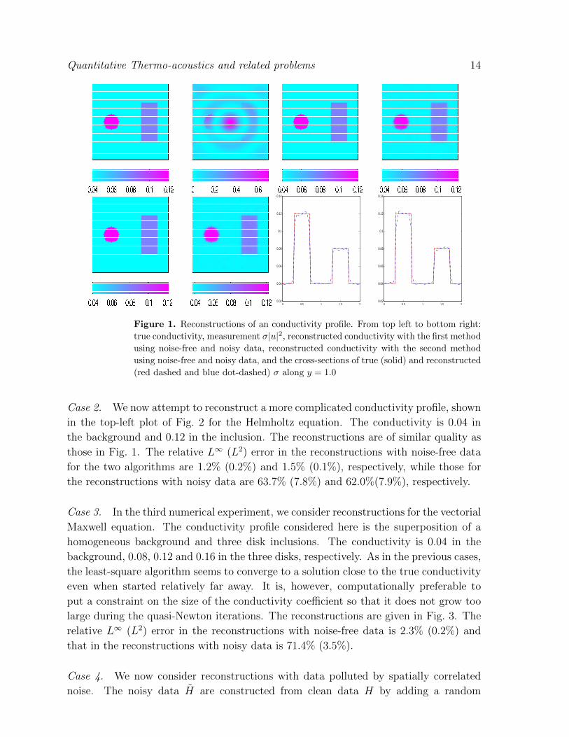
Case 1. We first consider the reconstruction of the simple conductivity profile

σ(x) =

0.12, x ∈ X1

0.08, x ∈ X2

0.04, x ∈ X\(X1 ∪X2)

(41)

where X1 = {x||x−(0.5, 1)| ≤ 0.2} and X2 is the rectangle X2 = [1.3 1.7]×[0.5 1.5]. The

true conductivity profile is shown in the top-left plot of Fig. 1. The synthetic data that

we have constructed is shown on the top-right plot of the same figure. We performed

four reconstructions. Two with noise-free data and two with noisy data that contain

10% multiplicative noise added by the algorithm H = H ∗(1+ α100

random) with random

a random field with values in [−1 1] and α the noise level. The reconstructions are given

the second and third row of Fig. 1. The relative L∞ (L2) error in the reconstructions with

data for the two algorithms are 1.5% (0.2%) and 1.5% (0.1%), respectively, while those

for the reconstructions with noisy data are 48.2% (2.9%) and 49.1%(2.9%) respectively.


0 0.5 1 1.5 20.02

0.04

0.06

0.08

0.1

0.12

0.14

0 0.5 1 1.5 20.02

0.04

0.06

0.08

0.1

0.12

0.14

Figure 1. Reconstructions of an conductivity profile. From top left to bottom right:

true conductivity, measurement σ|u|2, reconstructed conductivity with the first method

using noise-free and noisy data, reconstructed conductivity with the second method

using noise-free and noisy data, and the cross-sections of true (solid) and reconstructed

(red dashed and blue dot-dashed) σ along y = 1.0

Case 2. We now attempt to reconstruct a more complicated conductivity profile, shown

in the top-left plot of Fig. 2 for the Helmholtz equation. The conductivity is 0.04 in

the background and 0.12 in the inclusion. The reconstructions are of similar quality as

those in Fig. 1. The relative L∞ (L2) error in the reconstructions with noise-free data

for the two algorithms are 1.2% (0.2%) and 1.5% (0.1%), respectively, while those for

the reconstructions with noisy data are 63.7% (7.8%) and 62.0%(7.9%), respectively.

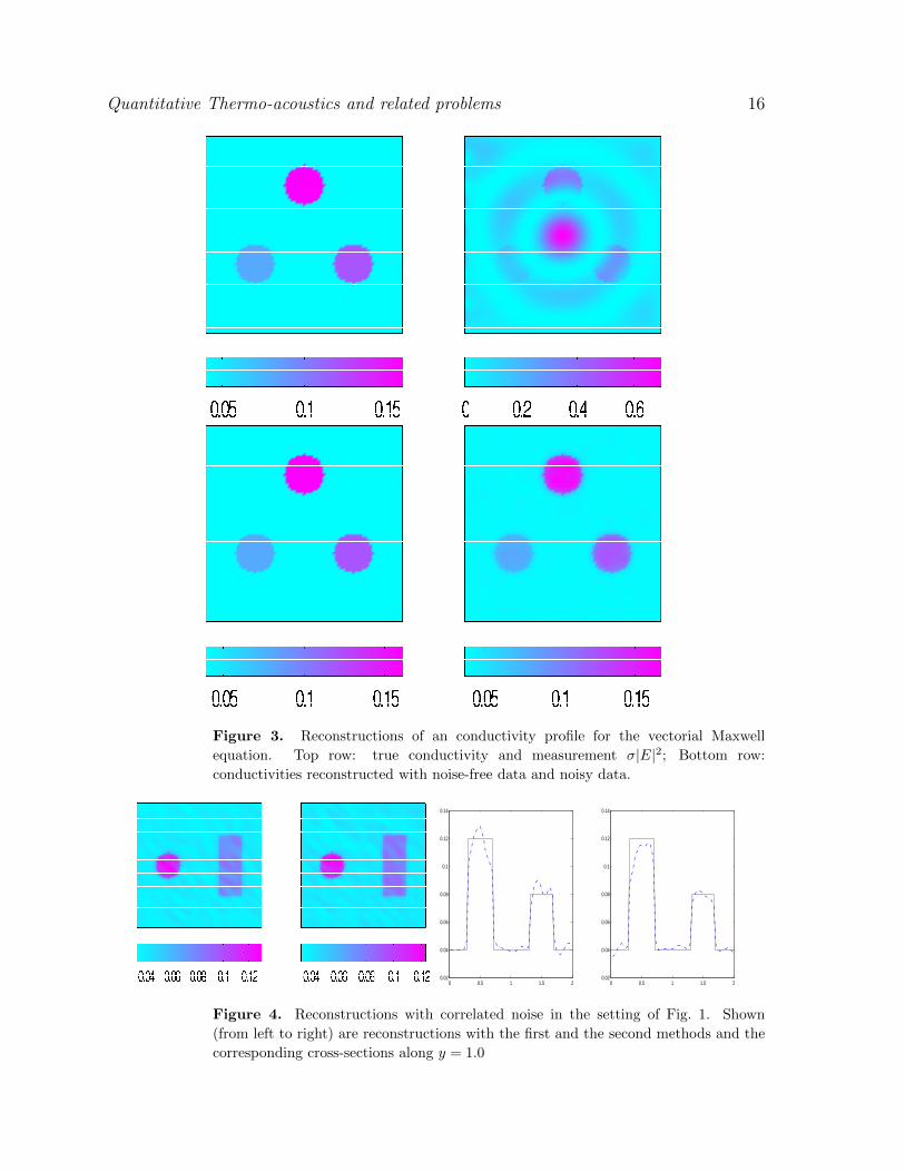
Case 3. In the third numerical experiment, we consider reconstructions for the vectorial

Maxwell equation. The conductivity profile considered here is the superposition of a

homogeneous background and three disk inclusions. The conductivity is 0.04 in the

background, 0.08, 0.12 and 0.16 in the three disks, respectively. As in the previous cases,

the least-square algorithm seems to converge to a solution close to the true conductivity

even when started relatively far away. It is, however, computationally preferable to

put a constraint on the size of the conductivity coefficient so that it does not grow too

large during the quasi-Newton iterations. The reconstructions are given in Fig. 3. The

relative L∞ (L2) error in the reconstructions with noise-free data is 2.3% (0.2%) and

that in the reconstructions with noisy data is 71.4% (3.5%).

Case 4. We now consider reconstructions with data polluted by spatially correlated

noise. The noisy data H are constructed from clean data H by adding a random


0 0.5 1 1.5 20.02

0.04

0.06

0.08

0.1

0.12

0.14

0 0.5 1 1.5 20.02

0.04

0.06

0.08

0.1

0.12

0.14

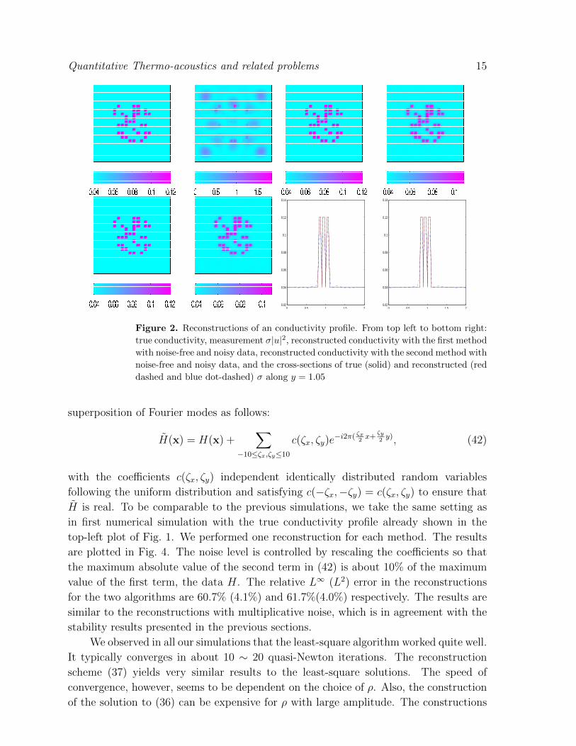
Figure 2. Reconstructions of an conductivity profile. From top left to bottom right:

true conductivity, measurement σ|u|2, reconstructed conductivity with the first method

with noise-free and noisy data, reconstructed conductivity with the second method with

noise-free and noisy data, and the cross-sections of true (solid) and reconstructed (red

dashed and blue dot-dashed) σ along y = 1.05

superposition of Fourier modes as follows:

H(x) = H(x) +∑

−10≤ζx,ζy≤10

c(ζx, ζy)e−i2π( ζx

2x+

ζy2y), (42)

with the coefficients c(ζx, ζy) independent identically distributed random variables

following the uniform distribution and satisfying c(−ζx,−ζy) = c(ζx, ζy) to ensure that

H is real. To be comparable to the previous simulations, we take the same setting as

in first numerical simulation with the true conductivity profile already shown in the

top-left plot of Fig. 1. We performed one reconstruction for each method. The results

are plotted in Fig. 4. The noise level is controlled by rescaling the coefficients so that

the maximum absolute value of the second term in (42) is about 10% of the maximum

value of the first term, the data H. The relative L∞ (L2) error in the reconstructions

for the two algorithms are 60.7% (4.1%) and 61.7%(4.0%) respectively. The results are

similar to the reconstructions with multiplicative noise, which is in agreement with the

stability results presented in the previous sections.

We observed in all our simulations that the least-square algorithm worked quite well.

It typically converges in about 10 ∼ 20 quasi-Newton iterations. The reconstruction

scheme (37) yields very similar results to the least-square solutions. The speed of

convergence, however, seems to be dependent on the choice of ρ. Also, the construction

of the solution to (36) can be expensive for ρ with large amplitude. The constructions


Figure 3. Reconstructions of an conductivity profile for the vectorial Maxwell

equation. Top row: true conductivity and measurement σ|E|2; Bottom row:

conductivities reconstructed with noise-free data and noisy data.

0 0.5 1 1.5 20.02

0.04

0.06

0.08

0.1

0.12

0.14

0 0.5 1 1.5 20.02

0.04

0.06

0.08

0.1

0.12

0.14

Figure 4. Reconstructions with correlated noise in the setting of Fig. 1. Shown

(from left to right) are reconstructions with the first and the second methods and the

corresponding cross-sections along y = 1.0


with CGO solutions is a useful theoretical tool. But they do not seem to provide better

numerical algorithms that standard least-squares algorithms for qPAT.

Acknowledgment

GB was supported in part by NSF Grants DMS-0554097 and DMS-0804696. KR was

supported in part by NSF Grant DMS-0914825. GU was partly supported by NSF,

a Chancellor Professorship at UC Berkeley and a Senior Clay Award. TZ was partly

supported by NSF grants DMS 0724808 and DMS 0758357.

References

[1] H. Ammari, E. Bossy, V. Jugnon, and H. Kang, Mathematical modelling in photo-acoustic

imaging, to appear in SIAM Review, (2009).

[2] G. Bal, A. Jollivet, and V. Jugnon, Inverse transport theory of Photoacoustics, Inverse

Problems, 26 (2010), p. 025011.

[3] G. Bal and K. Ren, Non-uniqueness results for a hybrid inverse problem, submitted.

[4] G. Bal and J. C. Schotland, Inverse Scattering and Acousto-Optics Imaging, Phys. Rev.

Letters, 104 (2010), p. 043902.

[5] G. Bal and G. Uhlmann, Inverse diffusion theory for photoacoustics, Inverse Problems, 26(8)

(2010), p. 085010.

[6] B. T. Cox, S. R. Arridge, and P. C. Beard, Photoacoustic tomography with a limited-

apterture planar sensor and a reverberant cavity, Inverse Problems, 23 (2007), pp. S95–S112.

[7] , Estimating chromophore distributions from multiwavelength photoacoustic images, J. Opt.

Soc. Am. A, 26 (2009), pp. 443–455.

[8] B. T. Cox, J. G. Laufer, and P. C. Beard, The challenges for quantitative photoacoustic

imaging, Proc. of SPIE, 7177 (2009), p. 717713.

[9] R. Dautray and J.-L. Lions, Mathematical Analysis and Numerical Methods for Science and

Technology. Vol.3, Springer Verlag, Berlin, 1993.

[10] D. Finch and Rakesh., Recovering a function from its spherical mean values in two and three

dimensions, in Photoacoustic imaging and spectroscopy L. H. Wang (Editor), CRC Press, (2009).

[11] S. K. Finch, D. Patch and Rakesh., Determining a function from its mean values over a family

of spheres, SIAM J. Math. Anal., 35 (2004),the cross-sections of true (solid) and reconstructed

(red dashed and blue dot-dashed) pp. 1213–1240.

[12] A. R. Fisher, A. J. Schissler, and J. C. Schotland, Photoacoustic effect for multiply

scattered light, Phys. Rev. E, 76 (2007), p. 036604.

[13] M. Haltmeier, O. Scherzer, P. Burgholzer, and G. Paltauf, Thermoacoustic computed

tomography with large planar receivers, Inverse Problems, 20 (2004), pp. 1663–1673.

[14] M. Haltmeier, T. Schuster, and O. Scherzer, Filtered backprojection for thermoacoustic

computed tomography in spherical geometry, Math. Methods Appl. Sci., 28 (2005), pp. 1919–

1937.

[15] Y. Hristova, P. Kuchment, and L. Nguyen, Reconstruction and time reversal in

thermoacoustic tomography in acoustically homogeneous and inhomogeneous media, Inverse

Problems, 24 (2008), p. 055006.

[16] V. Isakov, Inverse Problems for Partial Differential Equations, Springer Verlag, New York, 1998.

[17] R. Kowar and O. Scherzer, Photoacoustic imaging taking into account attenuation, in

Mathematics and Algorithms in Tomography, vol. 18, Mathematisches Forschungsinstitut

Oberwolfach, 2010, pp. 54–56.


[18] P. Kuchment and L. Kunyansky, Mathematics of thermoacoustic tomography, Euro. J. Appl.

Math., 19 (2008), pp. 191–224.

[19] C. H. Li, M. Pramanik, G. Ku, and L. V. Wang, Image distortion in thermoacoustic

tomography caused by microwave diffraction, Phys. Rev. E, 77 (2008), p. 031923.

[20] S. Patch and O. Scherzer, Photo- and thermoacoustic imaging, Inverse Problems, 23 (2007),

pp. S1–10.

[21] K. Ren, G. Bal, and A. H. Hielscher, Frequency domain optical tomography based on the

equation of radiative transfer, SIAM J. Sci. Comput., 28 (2006), pp. 1463–1489.

[22] J. Ripoll and V. Ntziachristos, Quantitative point source photoacoustic inversion formulas

for scattering and absorbing medium, Phys. Rev. E, 71 (2005), p. 031912.

[23] P. Stefanov and G. Uhlmann, Thermoacoustic tomography with variable sound speed, Inverse

Problems, 25 (2009), p. 075011.

[24] E. Stein, Singular Integrals and Differentiability Properties of Functions, vol. 30 of Princeton

Mathematical Series, Princeton University Press, Princeton, 1970.

[25] F. Triki, Uniqueness and stability for the inverse medium problem with internal data, Inverse

Problems, 26 (2010), p. 095014.

[26] M. Xu and L. V. Wang, Photoacoustic imaging in biomedicine, Rev. Sci. Instr., 77 (2006),

p. 041101.

[27] Y. Xu, L. Wang, P. Kuchment, and G. Ambartsoumian, Limited view thermoacoustic

tomography, in Photoacoustic imaging and spectroscopy L. H. Wang (Editor), CRC Press, Ch.

6, (2009), pp. 61–73.

[28] T. Zhou, Reconstructing electromagnetic obstacles by the enclosure method, Inverse Probl.

Imaging, 4(3) (2010), pp. 547–569.

quantitative thermo-acoustics and related problems · quantitative thermo-acoustics and related...

Documents