Quantum Computation

Jonathan A. Jones

Hilary 2010

Chapter 1

Principles of Quantum Computing

The purpose of this chapter is to provide a brief introduction to the fundamental principles un-derlying quantum computing: specific implementations will be considered in later chapters. For agood introduction to reversible computing see [RF96], while for quantum computing the standardtext [SS04] covers most of what you will need. The definitive text [NC00] is rather complicated; asan alternative try [ERD03].

1.1 Reversible computing

While quantum computation in its modern form is still a relatively young discipline1, researchershave been interested in the relationship between quantum mechanics and computing for a longtime. Early workers were not interested in the ideas of quantum parallelism, which will be exploredin the next section, but rather in the question of whether explicitly quantum mechanical systemscould be used to implement classical computations2. There are two technological reasons why thismight be considered an important question (beyond, of course, its intrinsic interest and amusementvalue).

The first reason is a direct consequence of Moore’s laws. After the development of integratedcircuits computing technology began its headlong dash down the twin roads of ever faster and eversmaller devices. These two phenomena are closely related: as computing devices must communicatewithin themselves, and as the speed of information transfer cannot exceed the speed of light, fastercomputers must indeed be smaller. Unfortunately there is a limit to this process, defined by theatomic scale: once the size of individual transistors becomes comparable with that of atoms the oldfashioned approach of micro-electronics becomes untenable. This limit is now being approached,but physicists were well aware of the existence of this limit long before reaching it became areal danger. The fundamental problem is that while macroscopic objects, such as transistors, aredescribed by irreversible physical processes, the behaviour of atoms and other very small objectsis essentially reversible3. Conventional computing, based on logic gates such as and and or is an

1The definition of “modern” quantum computation is largely a matter of taste, but in my opinion the field canbe traced back to a 1992 paper by Deutsch and Jozsa [DJ92].

2The key names in this field are Bennett [CHB73], Fredkin and Toffoli [FT82], and Landauer [RL82].3Recall that entropy and related ideas such as the arrow of time are essentially macroscopic concepts arising from

the statistical behaviour of large collections of microscopic objects.

1

apparently irreversible process, and it is not immediately obvious that it can be carried out at theatomic level. To overcome this it is necessary to show that computing can be carried out in anessentially reversible manner.

The second reason is closely related but more subtle. In addition to being made out of stuff,classical computers consume energy which they convert to heat. Our ever faster computers performthis transformation ever more rapidly, and modern computers suffer from the twin problems ofexcessive energy consumption (familiar as the short battery life of laptops) and excessive heatoutput (seen in laptops which are too hot to be used on laps). This problem could in principlebe completely overcome if (and only if) reversible computing is possible, as physically reversibleprocesses do not consume any energy4.

It is well known from classical irreversible computation that any desired logic operation can bebuilt from a network of and and not gates, and to prove that reversible computing is possible inprinciple it suffices5 to exhibit reversible versions of these gates. The not gate is easy, as this gateis intrinsically reversible; in reversible computing it is conveniently written as

ÂÁÀ¿»¼½¾ (1.1)

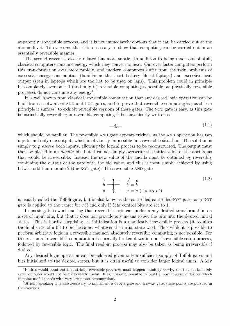
which should be familiar. The reversible and gate appears trickier, as the and operation has twoinputs and only one output, which is obviously impossible in a reversible situation. The solution issimply to preserve both inputs, allowing the logical process to be reconstructed. The output mustthen be placed in an ancilla bit, but it cannot simply overwrite the initial value of the ancilla, asthat would be irreversible. Instead the new value of the ancilla must be obtained by reversiblycombining the output of the gate with the old value, and this is most simply achieved by usingbitwise addition modulo 2 (the xor gate). This reversible and gate

a • a′ = ab • b′ = bc ÂÁÀ¿»¼½¾ c′ = c⊕ (a and b)

(1.2)

is usually called the Toffoli gate, but is also know as the controlled-controlled-not gate, as a notgate is applied to the target bit c if and only if both control bits are set to 1.

In passing, it is worth noting that reversible logic can perform any desired transformation ona set of input bits, but that it does not provide any means to set the bits into the desired initialstates. This is hardly surprising, as initialization is a manifestly irreversible process (it requiresthe final state of a bit to be the same, whatever the initial state was). Thus while it is possible toperform arbitrary logic in a reversible manner, absolutely reversible computing is not possible. Forthis reason a “reversible” computation is normally broken down into an irreversible setup process,followed by reversible logic. The final readout process may also be taken as being irreversible ifdesired.

Any desired logic operation can be achieved given only a sufficient supply of Toffoli gates andbits initialized to the desired states, but it is often useful to consider larger logical units. A key

4Purists would point out that strictly reversible processes must happen infinitely slowly, and that an infinitelyslow computer would not be particularly useful. It is, however, possible to build almost reversible devices whichcombine useful speeds with very low power consumptions.

5Strictly speaking it is also necessary to implement a clone gate and a swap gate; these points are pursued inthe exercises.

2

example is provided by reversible function evaluation, which for a function with two input bits andone output bit takes the form

af

a

b b

c ÂÁÀ¿»¼½¾ c⊕ f(a, b)

(1.3)

sometimes called a f -controlled-not gate. Clearly values of the function can be obtained by settinga and b to the desired inputs, and setting c = 0. Functions with more than one output bit can behandled by combining each output bit with its own ancilla.

1.2 Quantum parallelism

As we have seen, classical reversible computing can be achieved on a quantum computer by settingthe initial states of the qubits to eigenstates representing the desired inputs and then performingthe desired sequence of reversible logic gates. However quantum computers are capable of muchmore than this! Ultimately this comes from the fact that quantum operations are unitary, whichmeans they are both reversible and linear, and that quantum bits can be found in superpositionstates.

Consider a quantum network to evaluate a function f . If the input register is in an eigenstate|x〉 we can write this process as

|x〉|0〉 Uf−→ |x〉|f(x)〉. (1.4)

If the input register is in a superposition the result is trivially deduced by linearity. The ini-tial superposition state is a linear combination of inputs, and the resulting state will be a linearcombination of outputs:

N∑j=1

αj|xj〉|0〉 Uf−→N∑

j=1

αj|xj〉|f(xj)〉. (1.5)

Thus the quantum computer has effectively evaluated the function over all N inputs at the sametime! This effect, known as quantum parallelism, underlies all quantum algorithms. Note that ifthe input register comprises n qubits then it can be placed in a superposition of 2n states, andso the quantum computer can perform 2n calculations at once. While this is impressive, it is notimmediately clear how useful it is, and this point will be considered below.

Before doing this, I touch briefly on the question of universality of logic gates. As describedabove, the Toffoli gate is universal for reversible computing, meaning that any reversible logic canbe implemented using only Toffoli gates. Other universal gates6 are known, but like the Toffoligate they are all three bit gates, and it can be shown that a three bit gate is essential and thatuniversal computing cannot be achieved using only one and two bit reversible classical gates, such asnot and controlled-not. This appears to contradict a claim made earlier, that universal quantumcomputing can be achieved using only single qubit and two qubit gates. The solution to this paradoxis, of course that the Toffoli gate can be constructed out of single qubit and two qubit gates, but

6Such as the Fredkin (controlled-swap) gate, which swaps the values of two target qubits if and only if the controlqubit is set to 1.

3

only if these gates are not classical! For example a Toffoli gate can be implemented7 using twocontrolled-not gates, two controlled-square-root-of-not gates and one controlled-inverse-square-root-of-not gate. These last two gates can themselves be built out of controlled-notgates and single qubit gates such as the Hadamard gate.

1.3 Getting the answer out

Although quantum parallelism allows a quantum computer to simultaneously evaluate a functionover a vast superposition of inputs, it is not immediately clear that the result can actually be usedin any useful way, as it appears as a superposition of possible inputs and outputs. Suppose aquantum computer is prepared in the final state given in equation 1.5, and the values of the twoquantum registers are read out. Like any quantum measurement this can only result in one ofthe eigenstates of the measurement basis, and assuming that the measurement is performed in thecomputational basis then the result will be

|xj〉|f(xj)〉 (1.6)

for some value of j. The value returned will be chosen at random, with probabilities given by |αj|2as usual. Note that the values returned for the input and output will always correspond to thesame value of j, as the state before the measurement is an entangled superposition of inputs andoutputs.

As described above, a quantum function evaluation could be simulated by just evaluating thefunction over one input chosen at random; clearly this would not be very useful! The secret un-derlying effective quantum computation is that one does not measure the superposition of functionvalues directly; instead this is manipulated in cunning ways to produce an interesting result. To beuseful this process must combine the different values of f(xj) in a suitable fashion, so that the finalresult depends on all them. However, as the final measurement outcome can only be a single pairof numbers, this result cannot simply reveal the function values directly. Quantum computation isall about determining small pieces of information which depend on a large number of intermediateresults.

1.4 Deutsch’s algorithm

The invention of Deutsch’s algorithm can be taken as defining the start of modern quantum compu-tation8, and it remains a key example, exhibiting many of the key properties of quantum algorithmsin easy bite-size form.

Consider a binary function f from one bit to one bit, that is a function which takes in either 0or 1 as its input and returns either 0 or 1 as its output. There are four such functions

x f00(x) f01(x) f10(x) f11(x)0 0 0 1 11 0 1 0 1

(1.7)

7The explicit form is given in [SS04] and [ERD03].8The version of Deutsch’s algorithm described here is not in fact the original but a later modification which is

both more powerful and easier to understand.

4

which may be conveniently labeled as shown. These functions can be divided into two constantfunctions (f00 and f11), which have the same output for both inputs, and two balanced functions (f01

and f10), which have one output of 0 and one of 1. Equivalently, these functions can be classifiedaccording to their parity, defined as f(0)⊕ f(1).

Deutsch’s problem considers the determination of the parity of some unknown function f chosenfrom these four functions. It is assumed that the only way in which we can access this function isby the use of an oracle. This is just a fancy name for a black-box implementation of f which allowsus to investigate a function f by asking its value for some input x. The aim is to find the parity off with the smallest number of oracle calls9, that is the smallest number of queries10 about valuesof f(x).

In the language of quantum computing, this oracle must take the form of a propagator, whichperforms the transformation

|x〉|y〉 Uf−→ |x〉|y ⊕ f(x)〉 (1.8)

allowing the function to be evaluated in the usual reversible manner. This can be depicted as an(abstract) quantum circuit

|x〉Uf

|x〉|y〉 |y ⊕ f(x)〉

(1.9)

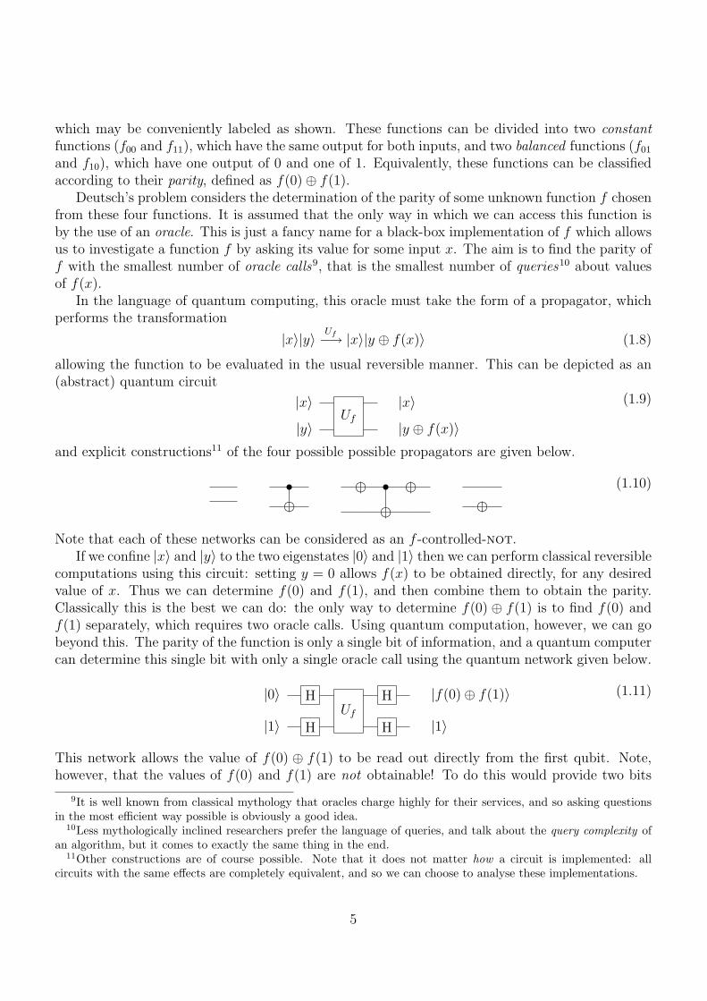
and explicit constructions11 of the four possible possible propagators are given below.

•ÂÁÀ¿»¼½¾

ÂÁÀ¿»¼½¾ • ÂÁÀ¿»¼½¾ÂÁÀ¿»¼½¾ ÂÁÀ¿»¼½¾

(1.10)

Note that each of these networks can be considered as an f -controlled-not.If we confine |x〉 and |y〉 to the two eigenstates |0〉 and |1〉 then we can perform classical reversible

computations using this circuit: setting y = 0 allows f(x) to be obtained directly, for any desiredvalue of x. Thus we can determine f(0) and f(1), and then combine them to obtain the parity.Classically this is the best we can do: the only way to determine f(0) ⊕ f(1) is to find f(0) andf(1) separately, which requires two oracle calls. Using quantum computation, however, we can gobeyond this. The parity of the function is only a single bit of information, and a quantum computercan determine this single bit with only a single oracle call using the quantum network given below.

|0〉 HUf

H |f(0)⊕ f(1)〉

|1〉 H H |1〉

(1.11)

This network allows the value of f(0) ⊕ f(1) to be read out directly from the first qubit. Note,however, that the values of f(0) and f(1) are not obtainable! To do this would provide two bits

9It is well known from classical mythology that oracles charge highly for their services, and so asking questionsin the most efficient way possible is obviously a good idea.

10Less mythologically inclined researchers prefer the language of queries, and talk about the query complexity ofan algorithm, but it comes to exactly the same thing in the end.

11Other constructions are of course possible. Note that it does not matter how a circuit is implemented: allcircuits with the same effects are completely equivalent, and so we can choose to analyse these implementations.

5

of information, and this requires two oracle calls12. The quantum algorithm merely provides anefficient way of answering a question; it does not perform the completely impossible.

So far I have simply asserted that this network will solve Deutsch’s problem: the next step isto show that it does so! This can be achieved in many different ways, and here I consider fourpossibilities in order of increasing sophistication.

The crudest approach is simply to work out what happens by direct matrix multiplication. Todo this we need a matrix description of the two qubit Hadamard

H(2) = H⊗ H =1

2

1 1 1 11 −1 1 −11 1 −1 −11 −1 −1 1

(1.12)

explicit forms for the four possible propagators

Uf00 =

1 0 0 00 1 0 00 0 1 00 0 0 1

Uf01 =

1 0 0 00 1 0 00 0 0 10 0 1 0

Uf10 =

0 1 0 01 0 0 00 0 1 00 0 0 1

Uf11 =

0 1 0 01 0 0 00 0 0 10 0 1 0

(1.13)and a description of the initial state

|01〉 =

0100

. (1.14)

The result then follows by direct multiplication. Note that this can be achieved either by multiplyingthe ket vector by each matrix in turn, or alternatively by multiplying the three matrices togetherfirst, and then applying the resultant matrix product to the ket vector. Both approaches haveadvantages, and it is not always immediately obvious which is the best approach in any particularcase.

A more interesting, approach is to consider the fate of the second qubit. This begins in |1〉which is converted to |−〉 by the first Hadamard. This then evolves according to

|0〉 − |1〉√2

Uf−→ |0⊕ f(x)〉 − |1⊕ f(x)〉√2

(1.15)

where x is the state of the first qubit. Now if f(x) = 0 this is just equal to |−〉, while if f(x) = 1it simplifies to

|1〉 − |0〉√2

= −|−〉 (1.16)

and so the process can be summarized as

|−〉 Uf−→ (−1)f(x)|−〉. (1.17)

12A more careful analysis of this algorithm suggests that the value of f(0), and thus the value of f(1), can beobtained from the phase of the final result. However this phase is a global phase, and thus not physically detectable.

6

The value of f(x) appears not in the value of the qubit, but rather in its phase. If this phase werea global phase then the information would in effect be lost, but this does not occur in Deutsch’salgorithm as the first qubit is also in a superposition state. Thus the algorithm begins with thesequence of transformations

|0〉|1〉 H(2)−→ |+〉|−〉 =|0〉|−〉+ |1〉|−〉√

2

Uf−→ (−1)f(0)|0〉|−〉+ (−1)f(1)|1〉|−〉√2

(1.18)

Note that the phase does not “belong” to the second qubit, but to the whole system, and canequally well be thought of as being applied to the first qubit13. Furthermore, the second qubit isalways in state |−〉, and this term can be factored out. Now if the function f is constant, so thatf(1) = f(0), equation 1.18 simplifies to

(−1)f(0) × |0〉+ |1〉√2

× |−〉 = (−1)f(0)|+〉|−〉 (1.19)

while if the function is balanced the result is

(−1)f(0) × |0〉 − |1〉√2

× |−〉 = (−1)f(0)|−〉|−〉. (1.20)

The initial phase term is a global phase and can be dropped. Finally, applying the last pair ofHadamard gates gives either |0〉|1〉 or |1〉|1〉 as appropriate.

The third approach is to combine the insights obtained from the second approach with knowledgeof the properties of gates. A little thought about the propagators Uf reveals that they all take theform of some combination of 11 gates (when f = 0) and X gates (when f = 1) applied to thesecond qubit, while the first qubit is left untouched. The effect of the Hadamard gates appliedto the second qubit before and after Uf is to convert this gate to an equivalent combination of 11and Z gates (since H11H = 11 and HXH = Z). Finally, applying a Z gate to a qubit in state |1〉 isequivalent to multiplying the state by minus one. Thus we can immediately deduce that the firstqubit undergoes the sequence of transformations

|0〉 H−→ |0〉+ |1〉√2

Uf−→ (−1)f(0)|0〉+ (−1)f(1)|1〉√2

H−→ |f(0)⊕ f(1)〉. (1.21)

Note that we do not need to explicitly write out the state of the second qubit at each stage: allthe states involved are separable and so it makes sense to talk about the state of the two qubitsindividually.

The final, and perhaps the boldest approach is to use operator identities to analyse the wholecircuit and only then consider the action on particular qubits. This can be done using explicitpropagator identities, or simply by using circuit identities to manipulate the circuits themselves.Thus, for example, the combined propagator for the case of f11 is given by

(H⊗ H).(11⊗ X).(H⊗ H) = (H.11.H)⊗ (H.X.H) (1.22)

13This effect, sometimes called phase kickback is very common in quantum computing.

7

which simplifies to 11⊗ Z using standard identities. In the same way the circuit for the case of f01

can be manipulated using circuit identities

H • H

H X H

=H • H

Z

=H Z H

•=

X

•(1.23)

and so the effect of applying Hadamard gates to both qubits before and after a controlled-notgate is simply to reverse the roles of control and target qubits. This greatly reduces the amount ofeffort, and examining the final circuits for the four possible functions

ÂÁÀ¿»¼½¾•

ÂÁÀ¿»¼½¾

• Z Z

(1.24)

allows the final results, including the global phases, to be calculated immediately. In the caseof Deutsch’s algorithm, however, it is not immediately obvious that this approach provides muchinsight into why it works,14 beyond explaining why it is essential that the second qubit begins instate |1〉.

1.5 Related algorithms

Deutsch’s algorithm is simple, but important, as it shows that a quantum device can find a propertyof an unknown function (its parity) with a smaller number of queries than any possible classicalalgorithm (one rather than two). For this reason we can say that quantum computing is moreefficient than classical computing within the oracle model of function evaluation15. The simplicityof the algorithm is also an advantage, as it permits it to be implemented on very primitive quantumcomputers. Beyond this, however, Deutsch’s algorithm is important as the simplest member of alarge family of quantum algorithms16, including most notably Shor’s quantum factoring algorithm.

The second simplest algorithm in the family is the Deutsch–Jozsa algorithm, which solves a veryclosely related problem. Consider an unknown binary function with n input bits, giving N = 2n

possible inputs, and a single output bit. For the case n = 1, which we analysed above, such functionsare always constant or balanced, but for n > 1 this need not be true: for example a function withN = 4 might return the value 0 for one of its inputs and the value 1 for the other three. Suppose,however, that the function is guaranteed to be either constant or balanced (useful but apparentlyarbitrary guarantees of this kind are usually called promises). Then the Deutsch–Jozsa problemis to determine whether the function is constant or balanced with the smallest number of queries(oracle calls).

14This approach is developed in some detail in [NDM08], and in some cases, most notably the Bernstein–Vaziranialgorithm, seems to provide a great deal of insight into how they work. The essential feature in these cases is onceagain the ability of Hadamard gates to interconvert control and target qubits; this is not, of course, possible withclassical computers as Hadamards are not permitted gates for classical bits.

15It is widely believed that quantum computing is more efficient than classical computing in general, but this is asurprisingly hard point to prove. Ultimately this question is related to the key question in computational complexitytheory of whether P is equivalent to NP; this is one of the seven Clay Mathematics Institute Millennium Problemsand has a prize of $1,000,000 on its head

16Formally speaking these algorithms tackle the Abelian hidden subgroup family of problems.

8

A little thought reveals that the best possible classical algorithm in this case is to simply tryinputs at random and compare the outputs. If any two different inputs give different outputs thenwe can immediately deduce that the function is balanced, but if all the outputs are the same it seemslikely that the function is constant. In this latter case we cannot be sure the function is constantuntil N/2 + 1 different inputs have been tried, by which time a balanced function is certain tohave revealed itself. Thus solving the Deutsch–Jozsa problem classically will require between 2(best case) and N/2 + 1 (worst case) queries17. Remarkably a quantum computer implementingthe Deutsch–Jozsa algorithm18 can always answer the question in a single query.

The Deutsch–Jozsa algorithm gets its power not just from the fact that quantum parallelism isused to evaluate the function for all its possible inputs in one step, but also from a final Hadamardtransform which combines these results in a cunning way. This final Hadamard transform is closelyrelated to a much more powerful operation, the quantum Fourier transform, or QFT. The details ofhow this works are beyond the scope of this course, but in essence the QFT extracts the frequencyof some periodic variation in the value of a function taken over all its inputs. A simple exampleis provided by the Deutsch–Jozsa algorithm which determines whether this frequency is zero (forconstant functions) or not (for balanced functions). A more complex example is Simon’s periodfinding algorithm; this underlies Shor’s method for efficient factorization which will be discussed atthe very end of this chapter.

1.6 Deutsch’s algorithm and interferometry

There is another interesting way of looking at Deutsch’s algorithm, which emphasizes the physicsrather than the mathematics. In essence there is an extremely close link between Deutsch’s algo-rithm and a Mach–Zender interferometer!

Consider a single photon which is incident on a beam splitter. As usual we treat the beamsplitter as a Hadamard gate, taking the photon from state |0〉 to the state H|0〉 = |+〉. The twophoton paths are then recombined at another beam splitter (Hadamard gate), and the final resultwill be H|+〉 = |0〉. Thus the photon will always emerge at the same port of the second beamsplitter. In effect we have reduced the traditional complex treatment of an interferometer to thetrivial observation that HH = 11.

Now suppose that we introduce phase shifters into the separated beam paths, which apply aphase shift of π, and so multiply a state by −1. If we introduce a phase shifter into the |1〉 path,then our state |+〉 will clearly be converted to |−〉, and the final output will be |1〉. If we introducea phase shifter into the |0〉 path then out state will be converted into −|−〉, and once again theoutput at the second beam splitter will be |1〉. Finally inserting phase shifters into both pathsconverts |+〉 to −|+〉, leading to an output of |0〉. Thus the output will be |1〉 if the phase-shifton the two paths is different, and |0〉 if the phase shift on the two paths is the same. The analogywith Deutsch’s algorithm is obvious.

17For the Deutsch problem N = 2 and these two limits are the same.18The full details of the Deutsch–Jozsa algorithm are beyond the scope of this course, but they can be found in

standard texts such as [SS04], [NDM08] or [NC00]. The case n = 2 (N = 4) is explored in the problem set.

9

1.7 Grover’s algorithm

Grover’s quantum search algorithm is an example of the second great class of quantum algorithms.The algorithm can be described in many ways, but the simplest approach is once again to considerthe analysis of binary functions.

Suppose we have a binary function f with n input bits and a single output bit, and we arepromised that f(x) = 1 for exactly one input, with f(x) = 0 for the remaining 2n − 1 inputs.19

Beyond this we know nothing about f , and can only obtain more information by making oraclequeries. The problem is to find the unique satisfying value of x for which f(x) = 1 with the smallestnumber of queries20. With a classical computer the only possible approach is to try different inputsat random until we find the unique satisfying input. If the number of possible inputs N = 2n issmall, then this process will be easy, but as n grows the process becomes extremely inefficient: onaverage it will be necessary to try around N/2 inputs, which for n = 32 means billions of queries.

Grover’s quantum search algorithm allows the satisfying input to be located much more rapidly,with about

√N queries. The general case is beyond the scope of this course, but the simple case

of n = 2 is relatively simple to analyze. In this case a classical search will require either 1, 2 or 3queries21 while Grover’s algorithm can guarantee to locate the satisfying input in a single query byusing the quantum network shown below.

|0〉 Hf

H ²±°¯©ª­® H

|0〉 H H ²±°¯©ª­® H

|1〉 H ÂÁÀ¿»¼½¾ H H ÂÁÀ¿»¼½¾ H

(1.25)

The first three qubit gate is an f -controlled-not gate, while the second one is similar to a Toffoligate but applies a not gate to the target bit if and only if both control bits are in state 0. (As usualthese three qubit gates can be built out of one and two qubit gates, but it is simpler to considerthem at this more abstract level.)

To simplify the analysis of this network begin with the last ancilla qubit. This behaves in verymuch the same way as the second qubit in the Deutsch algorithm, converting the f -controlled-Xgates into f -controlled-Z gates, and thus into phase shifts. As a result we can now ignore this qubitand concentrate our attention on the first two.

The first two qubits begin in the state |00〉 which is converted by the two qubit Hadamard gateinto a uniform superposition of the four possible inputs

|00〉 H(2)−→ |+〉|+〉 =|00〉+ |01〉+ |10〉+ |11〉

2. (1.26)

19It is conventional to label these functions by stating the value of the unique input for which the function is equalto 1, so, for example, f01(01) = 1 while f01(00) = f01(10) = f01(11) = 0. Note, however, that these four functionsfij are not the same as the four functions fij used in describing Deutsch’s algorithm.

20If you don’t like this mathematical description, then consider the problem of finding out someone’s name givenonly their telephone number and a copy of the relevant telephone directory.

21Note that it is never necessary to try all four inputs, as if the satisfying input has not been located in the firstthree attempts we know that the last input must be the one we are seeking.

10

The f -controlled-Z gate now evaluates the function simultaneously over all the possible inputs andapplies appropriate phase shifts to give the state

(−1)f(00)|00〉+ (−1)f(01)|01〉+ (−1)f(10)|10〉+ (−1)f(11)|11〉2

(1.27)

where, because of the promise about f , only one of the states will have a minus sign. To take aconcrete example, if the satisfying input is 01, then the state will be

|00〉 − |01〉+ |10〉+ |11〉2

. (1.28)

The desired satisfying state has now been picked out, and it might seem that the problemhas been solved, but a little more thought reveals that this is not in fact the case. Althoughthe satisfying state is uniquely labeled by its phase, it still contributes the same amplitude to thesuperposition as the other states, and so any attempt to measure the state of the first two qubitswill simply return one of the possible inputs at random. The purpose of the remaining gates is toconvert this phase difference into an amplitude difference. For the gory details see the problem set;for the moment it suffices to note that in the network above these gates will concentrate all theamplitude in the superposition on the desired state, so that a measurement of the first two qubitswill immediately reveal the satisfying input. If n > 2 this process cannot be achieved in a singlestep, and it is necessary to use a sequence of oracle queries and amplitude amplification steps, butthe quantum search is still much more efficient than its classical equivalent.

1.8 Quantum simulation

In addition to the period-finding algorithms (such as Deutsch and Shor) and the search algorithms(such as Grover) there is a third significant group of quantum algorithms based on quantum sim-ulation. The basic idea is to use a quantum computer to simulate the behaviour of another, morecomplex, quantum system. This may turn out to be the most important application of quantumcomputers in real life, but is beyond the scope of this course.

1.9 Error correction

The discovery of quantum error correction22 is one of the key developments in quantum computing,as it convinced many sceptics that quantum computing might just be possible. All computers arevulnerable to errors, but this is much more true of quantum than classical devices, as classicaldigital computers are inherently stabilised. Classical bits can only take the values 0 and 1, and ifthe physical implementation of the bit (such as a voltage) wanders away from its ideal value it canbe driven back. This is impossible for quantum computers for two reasons. Firstly qubits are notconfined to |0〉 and |1〉, but will be found in general superposition states. Secondly the processesthat drive a bit back to its ideal state are dissipative, and so non-unitary, while quantum evolutionmust be unitary.

22Made simultaneously by Peter Shor in the USA and Andrew Steane in Oxford

11

An alternative approach to handling errors is to use error correcting codes. For example it ispossible to encode a single logical bit by using code words made up of three physical bits, with 000representing the logical bit 0, and 111 representing logical 1. If any one physical bit is corruptedthis can be detected, as the three bits will no longer have the same value, and setting the singlebit that disagrees back to the consensus state will correct the error. A more careful analysis showsthat as long as bits become corrupted independently and with a small error probability this canprovide effective error suppression, and more complex schemes can give even better performance.

This classical scheme is useless in the quantum world, as it relies on repeatedly measuring thevalues of the physical qubits and comparing them. For qubits this will destroy the fragile quantuminformation stored in superposition states. The key realisation for quantum error correction is thatit is, however, possible to perform these measurements in such a way that the error is identifiedwithout damaging the superposition. To achieve this it is essential that the measurement onlyprovides information about the error, and provides no information at all about the state of thelogical qubit.

As a concrete example I will consider a system where one logical qubit is encoded in threephysical qubits, where one of the qubits may have been damaged by a spin flip error, that is one ofthe three qubits may have experienced an unintended not gate (X gate). For a detailed discussionsee [NC00] or [SS04], which use a slightly different language than that used here. As for the classicalcode, the two code words used are |0L〉=|000〉 and |1L〉=|111〉, and an arbitrary superposition stateis encoded as

|ψL〉 = α|0L〉+ β|1L〉 = α|000〉+ β|111〉 (1.29)

which can be achieved using either of the encoding networks shown below.

|ψ〉 • •|0〉 ÂÁÀ¿»¼½¾

|0〉 ÂÁÀ¿»¼½¾

|ψ〉 •|0〉 ÂÁÀ¿»¼½¾ •|0〉 ÂÁÀ¿»¼½¾

(1.30)

After the error process (we assume that at most one of the three physical qubits has been flipped)this state is converted to

|ψL〉 −→

α|000〉+ β|111〉 no error

α|100〉+ β|011〉 bit 1 flipped

α|010〉+ β|101〉 bit 2 flipped

α|001〉+ β|110〉 bit 3 flipped

(1.31)

depending on the exact form of the error. The task is to identify the error while learning nothingabout α and β. This can be achieved using the following network, which requires two additional(ancilla) qubits

• ••

•

|0〉 ÂÁÀ¿»¼½¾ ÂÁÀ¿»¼½¾NM

°°°

|0〉 ÂÁÀ¿»¼½¾ ÂÁÀ¿»¼½¾NM

°°°

(1.32)

12

where the bottom two qubits are the ancillas. Note that only the ancillas are directly measured,not the logical qubit! If no error has occurred then both ancillas will end up in state |0〉, while ifan error has occurred then either or both of the ancillas will end up in state |1〉. The first ancillacan only end up in state |1〉 if the physical qubits 1 and 2 have different values, while the secondancilla can only end up in state |1〉 if the physical qubits 1 and 3 have different values. By thismeans the error can be detected! A more complete analysis is left to the problem set.

A very similar approach can be used to correct for random phase flip errors, that is random Zgates, by using the code words |0L〉=| + ++〉 and |1L〉=| − −−〉. It is also possible to correct forboth sorts of error at the same time. The conceptually simplest approach is to use the nine qubitShor code which concatenates the two types of error correction described above [SS04, NC00]; moreefficient methods are also available but these are more complex to explain.

So far I have only considered gross errors, taking the form of X gates and Z gates, and havenot considered more subtle errors, such as small rotations around arbitrary axes. Remarkably themethods outlined above are sufficient to correct any such error. This point is briefly explored inthe problems.

1.10 Decoherence free subspaces

The key assumption about errors used in quantum error correction is that they are independent anduncorrelated, that is the probability of any one qubit being affected does not depend on what hashappened to other qubits. In practice, however, errors are caused by undesirable interactions withthe environment, and in many implementations it is likely that the errors will be highly correlated.23

This is a problem for quantum error correction, but can be exploited to give an entirely differentmethod of tackling errors, based on the idea of a decoherence free subspace or DFS.24

Once again the method relies on the use of code words. Here I will give a very simple descriptionof a subspace resistant to phase flip errors, motivated by implementations in NMR. (The treatmentin [SS04] goes beyond the scope of this course.) Consider the two code words

|0L〉 = (|01〉+ |10〉)/√

2 |1L〉 = (|01〉 − |10〉)/√

2 (1.33)

which are the ψ± Bell states. These are orthogonal quantum states, and so can be used to encodea logical qubit. They have the important property that

( |01〉 ± |10〉√2

)Z⊗Z−→ −

( |01〉 ± |10〉√2

)(1.34)

so that these states are invariant (neglecting an irrelevant global phase) under simultaneous Zrotations. Clearly a superposition of |0L〉 and |1L〉 will have the same property, and such a qubitwill be invulnerable to perfectly correlated phase decoherence. Invulnerability to correlated X

23Two qubits which are physically close in space will have similar environments and thus similar unwanted inter-actions.

24This method has the advantage that its implementation does not require projective measurements, and so itcan be used with techniques where this is difficult, such as NMR. Furthermore, error correction requires that errorsbe constantly detected and corrected, with gates being applied to every qubit in the system on a regular basis. Forlarge systems this means that gates must be applied in parallel. By contrast, the DFS approach aims to preventerrors from happening in the first place, and is intrinsically parallel.

13

rotations can be achieved using the two Bell states φ+ and ψ+ as the logical basis, and completeinvulnerability can be achieved using more complex codes25.

From the description above the decoherence free subspace approach looks like a magic bullet,but this is an overoptimistic view. The DFS approach only works if errors are perfectly correlated,and this is unlikely to be completely true in practice. In reality a DFS will only resist the correlatedpart of the errors, and if there are any significant uncorrelated errors these will soon build up. Forthis reason many researchers believe that the DFS approach should be combined with standarderror correction.

A second more subtle point is that it is necessary to implement quantum logic gates on thelogical qubits, rather than the physical qubits, which requires that much more complicated gates bedesigned. An alternative approach is to leave the DFS temporarily, while the gate is implemented,and return to it to allow the qubit to be stored. Both methods have been explored.

1.11 Quantum Factoring

Finally we turn to Peter Shor’s quantum factoring algorithm, which has driven the huge expansionin funding for quantum computers over the last decade. This algorithm has the potential to destroymany current forms of cryptography known as public key methods26. These schemes use a publickey, which is in essence the product of two very large prime numbers, and a private key, which isderived from the two numbers themselves. The security of the system is based on the apparentdifficulty of deducing the private key from the public key, and so is ultimately based on the beliefthat factoring large composite numbers is a difficult business27. All currently known factoringschemes on classical computers are inefficient, and it is widely believed that no efficient classicalalgorithm exists. By contrast, Shor’s quantum algorithm is known to be efficient, and so factoringwill become easy if a quantum computer is built.

Shor’s factoring algorithm is quite complicated [SS04], but the basic idea is fairly easy tounderstand. Given an unknown composite number N it does not seek to factor N directly, butsolves a closely related problem based on modular exponentiation. Begin by choosing a randomnumber a which is coprime with N , that is a number which shares no common factors with N .This check is easily made using Euclid’s efficient algorithm for calculating the greatest commondivisor (gcd) of a and N , as gcd(a,N) = 1 if the numbers are coprime28. Now consider the function

axmod N (1.35)

which has a period r, so that r is the smallest integer such that

armod N = 1. (1.36)

25Note that the encodings given above are not the only possible encodings for decoherence free subspaces. Thesimplest way to see this is to note that as general superpositions of |0L〉 and |1L〉 are decoherence free, then we canchoose any orthonormal pair of superposition states as our basis states. For simultaneous Z rotations a particularlysimple encoding is |0L〉 = |01〉 and |1L〉 = |10〉.

26Most notably the RSA system which is the basis of SSL, which underlies all electronic commerce on the internet.27As an exercise you might wish to try finding the two prime factors of the five digit number 19519 by hand. Now

imagine factoring a 200 digit number!28Note that the greatest common divisor of two numbers is also known as the highest common factor. Euclid’s

algorithm is based on the fact that gcd(x, y) = gcd(y, x mod y) for any two positive integers x > y.

14

Finding this period is exactly the sort of thing which quantum computers are good at! As describedin Chapter 1 a quantum computer can evaluate the modular exponentiation function for all possiblevalues of x and then use the quantum Fourier transform to pick out the period r.

The final stage of the algorithm relies on further results from classical mathematics called theChinese remainder theorem and Fermat’s little theorem. Briefly these can be used to show that ifr is even and if ar/2 mod N 6= N − 1 then at least one of the two numbers given by

gcd(N, ar/2 ± 1) (1.37)

is a non-trivial factor of N . If r does not have the required properties then one can simply pickanother value of a and try again. In fact it turns out that the process works for the majority ofpossible values of a, and so the Shor algorithm is very likely to work after a few tries.

15

Chapter 2

Experimental quantum computing

The previous chapter simply assumed that we had access to a general purpose quantum computerwhich we could use to implement our algorithms, and completely ignored how this might actuallybe done. We will soon consider three possible implementations in detail (trapped atoms and ionsthis term, and nuclear magnetic resonance in Trinity), but before doing so it is useful to considerthe problem in general.

2.1 The DiVincenzo criteria

Almost any physical system could be considered as a candidate for implementing quantum comput-ing, but to be a serious candidate a proposed system must have certain properties. The traditionallist of essential requirements was first described by David DiVincenzo, and his criteria provide auseful structure for discussions.

1. A scalable physical system with well-characterized qubits.

2. The ability to initialize the state of the qubits to a simple fiducial state, such as |0〉.3. Long relevant decoherence times, much longer than the gate operation time.

4. A universal set of quantum gates.

5. A qubit-specific measurement capability.

6. The ability to interconvert stationary and flying qubits.

7. The ability to faithfully transmit flying qubits between specified locations.

It is important to note that fulfilling these criteria is only necessary for proposals to build large-scale general-purpose quantum computers; small “toy” computers can be built with systems whichdo not do so. Furthermore, the last two criteria are not in fact required for quantum computersthemselves, but rather in order to build a “quantum internet”. However these criteria are importantif quantum devices are to be used to implement complex quantum communication protocols (to bedescribed next term) such as quantum teleportation.

16

2.2 The state of the art

At the current time there are no known physical systems which clearly fulfill all seven (or evenjust the first five) DiVincenzo criteria. A thorough summary of progress is provided by theARDA Roadmap 2004 [ARDA04], while a more up to date summary was published in Naturein 2008 [KS08].

However there are several system which fulfil some of these criteria well enough to make simpledemonstrations possible, and it is these that we will concentrate on. For quantum communicationit is clearly essential that criterion 7 be fulfilled; this is currently only really achievable for photons1,and unsurprisingly photons dominate this field. For quantum computation the one critical require-ment is criterion 4, a universal set of logic gates, as without this it is impossible to demonstrateany interesting algorithms. Here the field is led by trapped atoms and ions and by NMR2, whichwere introduced in the first part of this course, and it is these techniques which I will concentrateon. These are also the approaches which have been most actively pursued within Atomic and LaserPhysics in Oxford.

1Recent work on ions has shown that ion based qubits can be transported over short distances.2Well informed students would also include the recent work on one-way computing with photon cluster states,

but this is well beyond the scope of the current course.

17

Chapter 3

Trapped Atoms and Ions

As discussed in the first part of this course, a qubit can in principle be encoded using two energylevels in an atom or ion. In order to make this approach practical, however, it is essential to trapthe atom or an ion so that it can be held in a well controlled environment where it can be easilymanipulated. This can be achieved using electric and magnetic fields. For an extensive descriptionof this topic see [CJF05]; here I only consider the basics.

The use of trapped ions is one of the first proposals for building quantum computers, and stillone of the best developed (see [HRB08] for a detailed review of recent work). Proposals involvingtrapped atoms are slightly more recent, and have both substantial advantages and disadvantagesin comparison with trapped ions. These differences can ultimately be traced back to the fact thations interact strongly with their environment and have long range interactions with one another,while atoms interact more weakly and over shorter ranges. Comparing and contrasting the twoapproaches provides a useful general introduction to the problems underlying many other proposals.As usual I will structure the discussion around the first five DiVincenzo criteria, except that I willleave the question of scalability (that is, whether the technique can be scaled up to produce a largescale general purpose computer) to later.

3.1 Qubits

As mentioned above, the essence of the proposal is to encode the two qubit states |0〉 and |1〉 intwo different energy levels of an atom or ion. These levels are frequently referred to as |g〉 and |e〉,suggesting the ground state and some excited state, but the actual choice of levels is made so asto optimize the behaviour of the system, and it is common to use two hyperfine sublevels of theground state. A quantum computer must, of course, have more than one qubit, and this is achievedby using more than one atom or ion, with one qubit encoded on each physical object.

3.1.1 Ion traps

It is relatively easy to trap an ion as it will interact strongly with an electric field through theCoulomb interaction. Here I will assume that the ion is positively charged1. An obvious first idea

1This is usually the case in the systems we will think about; obviously negatively charged ions can be trapped ina similar way.

18

about how to trap it is simply to surround the ion with positively charged electrodes, each of whichwill repel it, so that it remains in the centre of the system. A little thought, however, immediatelyreveals that this process cannot be made to work. A trapped ion would obviously sit at a minimumof the electrostatic potential produced by the electrodes, and the existence of such a minimumwould violate Gauss’s law.

For example consider an arrangement of six positive charges, placed at equal distances on the±x, ±y and ±z axes from the ion, effectively forming an octahedron. For motion along the axesthe potential increases as the ion moves from the origin, and so it seems that this potential willconfine the ion. For motion between the axes, however, the potential decreases, and so the ion willbe expelled in one of these directions. Another example is to consider surrounding the ion with auniform sphere of positive charge. Naively one might guess that the ion would be repelled by thecharges towards the centre of the sphere, but elementary electrostatics shows that the electric fieldinside a uniformly charged sphere is in fact uniform, and thus the ion will feel no force at all.

It therefore appears that ion trapping is impossible! Fortunately this is not the case, and oneanswer is to replace the static arrangement of charges with a time-varying electric field2. This canbe done in such a way that the time averaged potential does indeed have a minimum at the centreof the trap. The process is quite complex (see [CJF05] for details) but a simple analogy can bemade with the situation of a ball sitting on a saddle shaped surface [WR95]. Clearly the ball istrapped in one direction but repelled in the other, and left alone the ball will simply fall off thesaddle. If, however, the saddle is made to rotate at the appropriate velocity then the rising edge ofthe saddle will “catch up” with the ball as it begins to fall, so that the ball remains trapped. Themathematics of the situation are equivalent to those found in the traditional Paul trap.

A more common design used for ion trap quantum computing is the linear Paul trap. Thisproduces a confining potential which is strong in two directions (x and y) and weak in the third(z). If two or more ions are placed in the trap they will repel one another through their mutualcoulomb interactions, and the final result will be a linear string of ions along the z axis. Thespacing between the ions can be controlled by varying the strength of the trap along this axis, andis typically around 10 µm.

So far I have assumed that the only effect of the trapping potential is simply to keep the ion (orions) in one place, but the real situation is much more complex than this. As the ion is confinedits motional states become quantized. This can usually be approximated by a harmonic oscillatorpotential, and so the energy levels of the trapped ion are replaced by ladders of energy levels. Thispoint is considered in more detail in the section on Initialization.

3.1.2 Atom traps and optical lattices

Atoms, unlike ions, are uncharged, and so cannot be trapped with electric fields. Instead they aretrapped using light. As before, I only describe the basic ideas here; the details can be found in[CJF05]. The most obvious approach is based on the scattering force which occurs when atomsabsorb photons coming from one direction and re-emit them at random, resulting in a net changeof momentum. When applied to atoms in an atomic beam, which are initially traveling in similardirections at similar speeds, this approach can be used to bring atoms almost to a halt. A moresophisticated approach, known as optical molasses uses six beams, one directed along each axis

2An alternative solution, adopted in the Penning trap, combines electrostatic and magnetic fields.

19

and all tuned slightly below a transition. The Doppler effect means that atoms will preferentiallyabsorb photons from the beam towards which they are traveling (these photons are blue-shiftedtowards resonance), and so atoms are effectively prevented from moving in any direction. Thiseffect is usually described as cooling the atoms, and while low temperatures can be reached thisapproach is limited by the Doppler cooling limit, which arises in essence from the fact that there isa minimum momentum transfer corresponding to the absorption of a single photon. Fortunatelythis limit can be surpassed by more complex sub-Doppler cooling techniques, ultimately leadingto an ultracold Bose–Einstein condensation. An even more powerful trap, known as a MagnetoOptical Trap or MOT, can be obtained by combining magnetic fields with circularly polarised laserbeams as described in [CJF05]. This allows large numbers of cold atoms to be stored for later use.

A more subtle form of optical trapping is based on the dipole force. The basic mechanism canbe easily understood by considering the forces on a prism which refracts a light beam. As thelight beam is bent, its momentum is changed, and so there must be a corresponding change in themomentum of the prism. Thus the prism feels a force, pushing it in the opposite direction to thelight beam. This force will depend on both the angle of the incoming light (as well as its intensityof course) and on the refractive index of the prism.

A similar situation occurs with an atom in a light field, except (of course) that an atom is notshaped like a prism! A better model is to treat the atom as a spherical lens, either focusing ordefocusing the light. If the light is of uniform intensity then there is no overall force on the sphere,but if the intensity varies then the sphere will feel a force that depends on the gradient of theintensity. Depending on the relative refractive index of the sphere, ηs, and the medium, ηm, thesphere will be pushed towards the region of highest light intensity (if ηs > ηm) or the region oflowest light intensity (if ηs < ηm). As the refractive index of a material changes substantially closeto an absorption line, the properties of the force will depend on the relative frequency of the lightand that of the relevant transition. This is the basis of optical tweezers which have found extensiveapplication in biophysics and nanotechnology.

This description is not really applicable to atoms, as refractive index is a property of bulkmaterials, but a proper mathematical treatment [CJF05] leads to similar results. The electric fieldof light can induce an oscillating dipole in an atom, which then interacts with the light field (hencethe name of dipole force). The magnitude of this force is greatest when the frequency of the lightis close to resonance, and its direction depends on whether the light is tuned above or below thetransition. In a spatially varying light field, atoms will seek either the regions of highest intensity orthose of lowest intensity, depending on the frequency of the light, allowing traps to be constructed.

This idea underlies the use of optical lattices to manipulate very large numbers of atoms inequally large numbers of traps. A standing wave laser field is created, which gives a light fieldwhose intensity varies periodically with a period equal to half the wavelength of the light. It turnsout that the dipole force is particularly effective in this arrangement, allowing atoms to be trappedin each well. With a little more effort a two (or three) dimensional standing wave can be created,giving a two (or three) dimensional array of these microtraps, sometimes described as an “eggboxfor atoms”.

The traps in these optical lattice are not very deep, and so can only trap cold atoms. This isachieved by loading them with atoms from a MOT or from a previously prepared Bose–Einsteincondensate. (The advantage of using a BEC is that the atoms are so cold that they end up in the

20

lowest vibrational state3 of the trap.) These atoms fill the traps at random, but they can be forcedto redistribute themselves evenly, so that exactly one atom ends up in each trap. The resultingarray of single atoms is known as a Mott-insulator state, and their internal states can be used asqubits.

3.2 Initialization

Having trapped the atoms or ions it is necessary to ensure that their qubits are all in some welldefined initial state, usually |0〉, before they can be used for a computation. If the two basis stateswere indeed a ground and excited state then this could be achieved by direct cooling, but in practicemore subtle mechanisms are required, and this is achieved through optical pumping. The basicidea is very simple: a laser is used to excite atoms which are in any state other than the desiredinitial state, and combined with random relaxation processes this leads to preferential populationof the desired state.

With trapped ions it is important to note that in addition to cooling the qubit itself, it is alsoimportant to cool the vibrational modes of the ions within the trap potential. This can be donein exactly the same way, a technique known as sideband cooling. For a simple explanation see[SS04]. With trapped atoms this cooling is built into the early stages of the trapping process whenan ultra-cold BEC is prepared.

3.3 Decoherence

Decoherence processes occur in any physical system, and are the great enemy of quantum informa-tion processing as they cause coherent superpositions to decay into classical mixtures. In essenceall decoherence can be traced back to uncontrolled interactions with the environment. A detailedtreatment is well beyond the scope of this course, but it is immediately obvious that long rangecoulomb forces may give rise to serious problems in trapped ions.

Tackling decoherence is also the fundamental reason for using two hyperfine levels within theground state, rather than a ground state and an excited state. The ultimate limit to decoherenceis provided by the spontaneous emission lifetime of a transition, and this decreases very rapidly forthe high energy transitions to excited states.

3.4 Universal logic

Clearly it is essential to be able to perform universal quantum logic if interesting computations are tobe achieved. As mentioned previously, it can be shown that the combination of the controlled-notgate and a small set of single qubit gates is indeed universal for quantum information processing,meaning that any desired operation can be built from a network of these gates; in particular threequbit gates (such as the Toffoli gate) are not required. This is a key result in experimental quan-tum information processing as directly implementing a three qubit gate would require a physical

3Strictly speaking the lowest Bloch band of the lattice, as the vibrational levels are split into a band by quantumtunneling between different traps.

21

interaction involving three particles: fortunately we only require interactions involving one or twoatoms or ions.

3.4.1 Single qubit gates

Single qubit gates are (in principle) simple for trapped ions, as these can be achieved using Ramantransitions induced by shining lasers on the ion of interest. By controlling the power, duration, andphase of the laser pulse a wide range of different single qubit rotations can be directly achieved,and any remaining single qubit gates required can be constructed out of networks of these basicgates. Of course, single qubit gates require that only one qubit experiences the rotation, but this isrelatively simple as the spacing between ions is large compared to the wavelength of the laser lightused, and so it is not too difficult to focus the lasers down onto single ions.

The situation with atoms trapped in optical lattices is more problematic. There is no problemin using Raman transitions to induce rotations, but selectively exciting a single qubit is extremelydifficult. The separation between individual atoms is usually only half a wavelength of the lightused to set up the lattice, making it impossible to focus on a single atom. Although methods totackle this can be imagined this is currently a major problem with trapped atoms. It is, however,easy to carry out simultaneous identical single qubit gates on very large numbers of trapped atoms,and this intrinsic massive parallelism is a topic of considerable interest in optical lattice research.

3.4.2 Two qubit gates (ions)

Next it is necessary to implement a two qubit gate, such as the controlled-not gate. It is importantto note that the controlled-not gate is not the only universal two qubit gate, and in fact any non-trivial two qubit gate4, and thus almost any physical interaction between the atoms or ions carryingthe qubit, can be used as the basis of universal logic.

For trapped ions it is simple to see how a gate can be built in principle, although the detailsof actually doing it in practice are quite complex. The basic interaction used is the Coulombrepulsion between ions, which links the motional degrees of freedom of the ions into commonvibrational modes. To put it crudely, if one ion in a trap is waggled the others will certainly notice.The basic idea is to use selective Raman transitions which excite motions in an ion if and only ifit is in the (qubit) excited state, in effect transferring the information stored in the superpositionfrom the qubit state into the vibrational state of the ion. Since the motion of all the ions is coupled,this information is now available at each and every other ion in the form of its own vibrationalstate. Thus the common vibrational mode acts as a “data bus”, carrying quantum informationbetween different ions and so between different qubits. A slightly more detailed description of themechanism actually used (the classic Cirac–Zoller gate) can be found in [SS04] or [ZCDG03], buta full understanding is specifically off-syllabus.

3.4.3 Two qubit gates (atoms)

This approach cannot be used with trapped atoms, as they do not have the long range Coulombinteractions required. It is possible to use dipole–dipole interactions between induced electric

4To make this statement useful it is necessary to give a better definition of trivial, or equivalently non-trivial. Onesimple approach is to note that any gate which can convert a product state into an entangled state is non-trivial.

22

dipoles, but here I concentrate on another interaction, the contact or collision interaction.Although atoms do not normally interact strongly at long distances, they repel each other very

strongly at short distances, so that it is not possible to squeeze two atoms into the space normallyoccupied by one. The micro traps in optical lattices are so small that this effect can be quitesignificant, and so the energy of an atom in a trap will depend on whether or not there is anotheratom in the same trap. In general, the act of bringing two atoms closer together will raise theirenergy, and therefore (by the time-dependent Schrodinger equation) cause them to pick up anadditional phase shift, beyond that which they would have acquired if left alone. Note that to agood approximation only the energies of the atoms are changed, and not their wavefunctions, asexpected from first order perturbation theory.

Detailed calculations of the strength of the contact interaction are quite complex, but the keyresults are fairly simple. As the interatomic potential is usually short range only head-on collisionsmatter, and so the collision can be described using s-wave scattering, in which the relative orbitalangular momentum of the colliding particles is assumed to be zero. In this case the interactionturns out to be describable by a single parameter, the scattering length a. The energy shift arisingfrom the collisional interaction between two identical atoms of mass M is then approximately givenby

Ea =4π~2 a

M

∫|ψ|4 dr (3.1)

where ψ is the vibrational wavefunction of the atom in the trap. The fourth power dependence onψ corresponds to a quadratic dependence on the probability of the atom being found at some pointin the well, and so the integral gives the probability of two atoms being found at the same pointin space. Clearly this depends strongly on the shape of the trapping potential. Note that althoughthe scattering length has the dimensions of length it does not simply correspond to the atomic size:it can vary greatly with fine details of the situation, and can even be negative. For a slightly moredetailed treatment see [CJF05].

If two atoms are made to collide for a time τ , the system picks up an additional phase shifte−iφ, with φ = Eaτ/~. To implement a controlled logic gate with this interaction it is necessaryto make the additional phase shift depend on the qubit state of the two atoms involved. This canbe achieved by making the trapping potential depend on the qubit state, so that atoms in state|0〉 will feel one potential, while atoms in state |1〉 will feel a different potential. If these potentialscan be controlled independently, then atoms can be moved in different ways depending on theirqubit state. Since this whole process is quantum mechanical, an atom whose qubit is in a coherentsuperposition of both |0〉 and |1〉 will move in both directions at once!

This effect can be achieved when the qubit corresponds to the mS = ±12

spin states of the S1/2

ground state of an atom such as Rb. In this case the laser frequency can be chosen such that the ±12

spin states interact with the σ± components of the standing light wave, and these can be controlledby varying the phase of the light. In particular, it is possible to arrange that the σ+ traps, andthus the mS = +1/2 atoms, are moved in one direction, while the σ− traps (mS = −1/2 atoms)are moved in the other direction. If this process is applied to an optical lattice filled with atoms,the consequence is that atoms moving in one direction will collide with those moving in the otherdirection. The optical lattices can then be moved back to their original positions, and the atomswill end up where they started, except that those atoms which have collided will have picked upan additional phase.

23

For example consider the simple case of two atoms in neighboring traps, and suppose that thelattices are adjusted in such a way that atoms in state |0〉 move right, while those in state |1〉move left. If the atoms are numbered from left to right, then a collision will only occur if the firstatom moves right (and so is in state |0〉) and the second atom moves left (and so is in |1〉). Thusthe overall evolution (neglecting global phases and any background evolution due to the ordinaryenergy difference between |0〉 and |1〉) is

|00〉 → |00〉 |01〉 → e−iφ|01〉 |10〉 → |10〉 |11〉 → |11〉 (3.2)

which is a phase gate

Uφ =

1 0 0 00 e−iφ 0 00 0 1 00 0 0 1

. (3.3)

Choosing φ = π gives a gate very similar to the controlled-Z gate, and it is not surprising that thisgate is a universal two qubit logic gate.

It is important to note that there are several possible ambiguities in the definition of phasegates, both within the optical lattice literature, and also comparing this with other techniques.Firstly, there is some variation as to whether there is a plus or minus sign in front of the phaseshift, and secondly there is very considerable variation as to which state the additional phase isapplied to. Finally, some treatments explicitly include the ordinary background evolution. None ofthis is ultimately very important, as all these definitions are related by simple single qubit gates.Nevertheless, it is necessary to keep a careful eye out. It is also important to recall that collisiongates are coherent processes, and so the same description can be applied to atoms in superpositionstates, as we will explore next.

3.4.4 Massive entanglement

In the discussion above I only considered a pair of atoms. It is easy to see that entanglement canbe generated in such a system. For example

|00〉 H(2)−→ |+〉|+〉 = (|00〉+ |01〉+ |10〉+ |11〉)/2Uπ−→ (|00〉 − |01〉+ |10〉+ |11〉)/2

= (|0〉|−〉+ |1〉|+〉)/√

2

(3.4)

which is a maximally entangled Bell state, even if it is written in a slightly unusual basis. It couldbe converted to a conventional Bell state by applying a Hadamard gate to either of the two qubits,but this is difficult in an optical lattice as the two atoms are very close together.

The situation becomes even more interesting in lattices containing very large numbers of atoms.Since both the single qubit gates and the two qubit entangling gates are applied to all the qubits inparallel, this provides a simple route to extremely large entangled states, known as cluster states.

24

For three atoms the phase gate looks like

Uπ =

1 0 0 0 0 0 0 00 −1 0 0 0 0 0 00 0 −1 0 0 0 0 00 0 0 −1 0 0 0 00 0 0 0 1 0 0 00 0 0 0 0 −1 0 00 0 0 0 0 0 1 00 0 0 0 0 0 0 1

(3.5)

and the entangling transformation performs

|000〉 H(3)−→ Uπ−→ (|000〉 − |001〉 − |010〉 − |011〉+ |100〉 − |101〉+ |110〉+ |111〉)/2√

2

= (|+〉|0〉|−〉 − |−〉|1〉|+〉)/√

2(3.6)

which is an example of a class of three qubit entangled states called GHZ states. With largernumbers of qubits the resulting states are very complex and are called cluster states; a moresophisticated way of describing these states is hinted at in the problems. Even more interestingbehaviour can occur in multidimensional optical lattices, as in this case it is possible to moveatoms not just left to right, but also back to front and up and down, permitting much morecomplex interactions.

The result of these processes is often called massive entanglement, and is interesting for manyreasons. Firstly, optical lattices provide one of the simplest routes to extremely large entangledstates, which are important when studying the transition between quantum and classical physics.Secondly, the detailed form of the entangled states produced turns out to be surprisingly useful, withobvious applications in three areas of quantum information processing, namely error correction,quantum simulation, and the implementation of so-called “one-way” quantum computers. Thedetails of these topics are, however, beyond the scope of this course.

3.5 Readout

The final stage which must be considered in any proposed implementation of a quantum computeris, of course, readout: there is no point in running a quantum computation if the final result cannotactually be obtained. This final stage is relatively simple with ion traps, as it is possible to measurethe quantum states of ions with accuracy and selectivity. The basic idea is to detect the fluorescencefrom the ion using optical transitions.

This might seem impossible, as the qubit is deliberately implemented using two levels whichdo not fluoresce: if they did then they would swiftly relax and the quantum information would bedestroyed! The solution is to use a laser to drive the atom from one of the qubit states (usually|0〉) to a third level, which does fluoresce strongly. The simplest situation occurs when the thirdlevel decays back to |0〉, an example of a cycling transition. In this case strong fluorescence will beseen5 at the driving frequency if and only if the qubit is in state |0〉. For a superposition state

|ψ〉 = α|0〉+ β|1〉 (3.7)

5It is literally possible to see a single fluorescing ion with the naked eye.

25

this acts as a projective measurement: the system shows fluorescence, and ends up in state |0〉 withprobability |α|2, while no fluorescence is seen, and the atom ends up in state |1〉, with probability|β|2.

It is, of course, possible to use very similar methods with trapped atoms, but with opticallattices the characteristic problem of distinguishing between different atoms remains. Individualions in a trap can be distinguished by their positions using a simple microscope, but atoms in anoptical lattice are much closer together. It is also not really practical to focus the driving laser on asingle atom in a lattice. This makes selective readout just as difficult as selectively applying gates.

26

Chapter 4

Nuclear Magnetic Resonance

Liquid state nuclear magnetic resonance (NMR) is little studied in the standard Oxford Physicscourse1 but has recently become of considerable interest as a method for building small quantumcomputers. The underlying ideas were introduced in the first part of this course, but these werelimited to systems with a single nuclear spin, and thus a single qubit; here we expand these ideasto cover systems with two or more qubits. For a more detailed discussion see [SS04]; for the realdetails see [JAJ03].

4.1 Qubits

The basic idea behind NMR QC is that the two spin state of a spin-1/2 nucleus provide a naturalimplementation of a qubit: indeed it is such a natural implementation that a qubit is often referredto as a spin. To obtain more than one qubit, just use more than one spin. There are, however, flawsin this naive approach, which can be traced back to the low frequencies (and thus low energies) ofNMR transitions,

∆E = hν = ~γB (4.1)

where γ is a constant characteristic of the nucleus called the gyromagnetic ratio. This energy gaparises from the Zeeman interaction of the nuclear spin with an externally applied magnetic field,and for reasonably accessible field strengths (up to around 20 T) lies in the range up to 1 GHz.

4.1.1 Qubit selection

While these low frequencies make experiments very easy, the corresponding long wavelengths meanthat it is impossible to directly distinguish between different nuclei according to their positions inspace. Instead it is necessary to use the different transition frequencies observed for different nucleifor qubit selection. This is easy as long as different qubits are represented by different nuclearspecies, as these have different gyromagnetic ratios, leading to very different frequencies. However,there are only a small number of distinct spin-1/2 nuclei available, and a computer of any reasonable

1Its sole appearance outside C2 is in the practical SS14 (based on an approach to NMR which has been obsoletefor more than 40 years) and the short option S10 (which includes Magnetic Resonance Imaging). References tonuclear magnetic resonance in physics texts often refer to the molecular beam experiments by Rabi more than 60years ago.

27

size will have to represent several different qubits with the same nuclear type. Fortunately the exactfield experienced by a nucleus is not simply equal to the externally applied field, but also dependson local fields. Roughly speaking, the external field induces a current in the electrons surrounding anucleus; this current produces an additional field which acts to shield the nucleus from the appliedfield. These shielding effects, and thus the value of the transition frequency, will depend on thedetails of the nuclear environment, an effect known as the chemical shift.

It is in principle possible to use the methods of Magnetic Resonance Imaging (MRI) to makethe transition frequency depend on the spatial position of a nucleus, and this approach has beenconsidered. However, the spatial resolution required goes far beyond that normally achieved, andthis approach seems very difficult in practice.

4.1.2 Ensembles

A second problem of the low frequencies is that the energy of the corresponding photons (a fewµeV) is so low that it is not currently practical to detect a single radio frequency photon. Thus wecannot detect a single nuclear spin, and instead have to use an ensemble of identical independentnuclei. This greatly limits the range of systems available to us, and as we will see has very significantconsequences for both initialization and readout.

4.1.3 Molecules in liquids

The solution adopted in most NMR QC studies to date is to use fairly dilute solutions of smallmolecules in inert solvents2. Each molecule will contain a number of different spin-1/2 nuclei, eachof which can be used as a qubit. As every molecule is chemically identical, there are a very largenumber of copies of the quantum computer, and the experiment controls these in parallel3. Itmight seem that different molecules would in fact be subtly different (due to effects such as internalmotions and the orientation of the molecules with respect to one another and the applied field),but all these effects are averaged out by the rapid molecular tumbling which occurs in solution.Furthermore, it turns out that the interactions between spins in different molecules are averagedout by the same tumbling process, and so molecules in liquids provide an ensemble of identicalindependent copies, as required.

4.2 Initialization

The obvious method to initialize a spin system is simply to cool the spins directly into theirthermodynamic ground state4. However a comparison of the transition energy (say 1 µeV) with kTat room temperature (around 25 meV) reveals that this approach will require temperatures around1 mK. This temperature is perfectly attainable, but clearly not for solutions of small molecules.

There are three potential ways around this problem. The first is to switch to NMR studies ofsolid state systems, where direct cooling may be practical. The second is to find some cunning

2There have been some NMR QC studies involving solid state systems or more complex systems such as liquidcrystals, but these are not considered further here. See [JAJ03] for a brief discussion.

3Recall that there is effectively no spatial discrimination in NMR experiments.4Since a spin-1/2 particle is a natural qubit there is no question about cooling into one specific sub-level.

28

method to obtain a non-equilibrium population of the spin states. The third is, quite simply, tocheat! With ensemble systems it is possible to use so-called pseudo-pure states, which appear tobehave like pure states. All three approaches have been used, but the method of pseudo-pure statesis by far the most common.

4.2.1 Pseudo-pure states

The method of pseudo-pure states relies on two basic concepts to generate a state which appearsto behave like a pure state. The first fact is that it is possible to use a combination of unitaryand non-unitary operations to convert the thermodynamic equilibrium state of a spin system intoa state where all the different energy levels have the same population, except for the ground levelof the whole system which has a slightly higher population. The second fact is that the NMRexperiment is not sensitive to spin systems where all the levels have the same population, so thatthe only signal actually observed from this state arises from the small excess population in theground level. Thus the large ensemble of spins in a highly-mixed state gives the same result as amuch smaller ensemble of spins in a pure state.

To take a concrete example consider a molecule containing two spin-1/2 nuclei, each of thesame nuclear species and with small interactions such as the chemical shift ignored. The Zeemaninteraction means that the ground level |00〉 will lie at an energy hν below the unsplit position,while the level |11〉 will lie at hν above the unsplit position. The two levels |01〉 and |10〉 will bedegenerate at the original energy. Clearly the state |00〉 will have the largest population at thermalequilibrium, but the population differences will be small. In the high temperature limit kT À hν,which applies in liquid state NMR, the fractional populations can be written as 1/4 + ε, 1/4, 1/4,and 1/4− ε, with ε ∼ 10−5, and the resulting density matrix of the system is

ρB =∑

j

Pj|j〉〈j| =

1/4 + ε 0 0 00 1/4 0 00 0 1/4 00 0 0 1/4− ε

(4.2)

while the desired pure state is

ρ00 = |00〉〈00| =

1 0 0 00 0 0 00 0 0 00 0 0 0

. (4.3)

The method of pseudo-pure states works by averaging the populations of all the levels except |00〉,and for details of how this is done see [SS04]. The resulting state is

ρPP =

1/4 + ε 0 0 00 1/4− ε/3 0 00 0 1/4− ε/3 00 0 0 1/4− ε/3

= (1/4− ε/3)×

1 0 0 00 1 0 00 0 1 00 0 0 1

+ (4ε/3)× ρ00

(4.4)and since the first term is not observable this state looks just like a pure state, except that thesignal is only 4ε/3 times as large as the signal from a true pure state.

29

The pseudo-pure state approach works well with small spin systems, but has major problemswhen applied to larger spin-systems. This point will be discussed in more detail later.

4.3 Decoherence

At first glance it seems that decoherence should not be a major problem for NMR quantum com-puting. The ultimate limit is provided by the spontaneous emission lifetimes of the spin states, andthese are around 109 years. Real systems are not quite so extreme, as NMR relaxation is dominatedby stimulated emission and absorption, arising from random fluctuations in a spin’s environment,but relaxation times for spin-1/2 nuclei are still very long, typically around 1 s.

This coherence time is greater than that usually observed in trapped atoms and ions, but thisis not as important as it might seem. While the long coherence time makes experiments relativelysimple, what matters for quantum computation is not the coherence time itself, but rather the ratioof the coherence time to the gate time. This ratio determines the number of gates which can beperformed before the system has decohered away, and NMR gates are also very slow in comparisonwith those in systems of trapped atoms or ions.

A more subtle advantage of NMR is that the use of ensemble systems means that decoherenceappears differently in NMR quantum computers than in other systems. In a conventional quantumcomputer decoherence introduces the possibility that the the computer will make some randomtransition, and so return the wrong answer at the end of the computation. In ensemble computers,however, different members of the ensemble can return different answers, with the observed resultbeing an average over the whole ensemble. With luck the wrong answers produced by decoherencewill largely cancel out, so that it appears simply as a reduction in the signal strength rather thanas an actual wrong answer. Real life is rarely quite so kind, but there is some truth in this idea.

4.4 Universal Logic

As usual, the problem of implementing universal logic comes down to the problem of implementingsingle qubit and two qubit gates. Single qubit gates can be implemented using resonant radiofrequency pulses, and this topic was considered in detail in the first part of this course. The onlysubtle points arise from the problem of applying these gates to individual qubits, rather than thewhole spin system, and here I simply assume that frequency selection can be achieved.

4.4.1 Spin–spin coupling

Two qubit gates are much more interesting, as these require some sort of spin–spin interaction.The obvious source is the direct interaction between the magnetic dipoles of two nuclei, but thisinteraction depends on the angle between the internuclear vector and the magnetic field, and iscompletely averaged out by rapid molecular tumbling (this is in essence the reason why differentmolecules can be treated as being independent of one another). The key interaction in liquid stateNMR studies is scalar coupling, also known as J-coupling. This is closely related to the electron–nuclear hyperfine interaction, and is mediated between different nuclei by shared valence electronswithin the molecule. The key result is that the J-coupling interaction does survive molecular

30

tumbling, and provides a coupling between spins in the same molecule. However, because it is acorrection to the direct coupling term, it is typically rather small (rarely more than 500 Hz).

The scalar coupling naturally has the Heisenberg form expected for an exchange interaction

σ1 · σ2 = σ1xσ2x + σ1yσ2y + σ1zσ2z (4.5)

but in most situations is truncated to the Ising form σ1zσ2z by the larger Zeeman interactions.This is nothing more than first order perturbation theory, where a small perturbation is seen tohave little or no effect on the eigenstates of a system, while slightly shifting the eigenvalues (energylevels). Thus the overall Hamiltonian of a two spin system can be written as

H/~ = ω1σ1z

2+ ω2

σ2z

2+ ω12

σ1zσ2z

2(4.6)

where energies have been written in angular frequency units as usual, and the factors of 12

arenecessary as ~ω is the energy gap between the ±1

2states, not the shift of the individual states.

Note that many treatments of NMR QC use traditional NMR conventions, where the ~ is simplydropped and Pauli matrices are replaced by other operators which are equivalent up to a constantfactor, so the exact form of the Hamiltonian can seem quite variable.

4.4.2 Spin echoes and refocusing

This Hamiltonian contains a spin–spin interaction, and so in principle will permit universal quantumcomputation, but the form is rather more complicated than one might wish, and it would be nice tobe able to “sculpt” it into a more desirable form. This can be achieved with spin echoes, which werediscussed in detail for single qubit systems at the start of this course. The basic idea is to allow thesystem to evolve under a Hamiltonian for a time τ/2, apply a not gate, allow the system to evolvefor another time τ/2, and then apply a final not gate (this final not gate is not always included,but it makes the overall analysis slightly simpler). In a single qubit system this will refocus theevolution under the Zeeman splitting (rotation around the z-axis at the Larmor frequency). Asimple way to think about this is that by interconverting |0〉 and |1〉 the not gate causes the spinto precess backwards during the second τ/2 time period.

In a two qubit system several different spin echoes are possible, as not gates can be applied toeither or both of the two spins. The effect on the Zeeman terms is obvious, and each of these willbe refocused if a pair of not gates is applied to the corresponding spin. It only remains to considerwhat happens to the spin–spin coupling. If a pair of not gates is applied to one of the two spins,then the coupling will also be refocused in the same way. If, however, not gates are applied toboth spins then the coupling is unaffected by the not gates, and so its evolution adds up duringthe whole spin echo. In effect, the not gates applied to one spin reverse the coupling evolutionduring the second τ/2 period, but the not gates applied to the other spin reverse it again, leavingit overall unaffected. Thus the effect of the spin echo is equivalent to evolving under the averageHamiltonian

Hav/~ = ω12σ1zσ2z

2(4.7)

for the whole time period τ .

31

In a multi-spin system there will in principle be couplings between all the pairs of nuclei, andso the Hamiltonian takes the general form

H/~ =∑

j

ωjσjz

2+

∑

j>k

ωjkσjzσkz

2. (4.8)

Using more complex patterns of spin echoes it is possible to sculpt the Hamiltonian almost at will,refocusing undesired terms while keeping those that are wanted. For the details see [JAJ03].

It might seem that a NMR quantum computer would require every spin to be directly coupledto every other spin, but this is in fact not the case. It is, however, necessary that every spin bedirectly or indirectly coupled to every other spin, where indirect coupling means that two spins areconnected to one another through a chain of directly coupled intermediate spins. For example, alinear chain of spins, each of which is coupled to its immediate neighbours, is sufficient. To seethat this is true, note that a (logical) qubit can be moved around the (physical) spin system usingquantum swap gates, so that any two qubits can be made to interact even if there is no directcoupling between the spins they are currently located on.

4.5 Readout

The basic readout mechanism used in NMR quantum computing is to acquire an NMR spectrum. Aswe will see, this ensemble process is quite different from the conventional projective measurementsthat are normally discussed in quantum mechanics, and this has significant consequences. Beforediscussing this, however, it is useful to consider the basic form of the NMR spectrum.

4.5.1 NMR spectra

I begin by considering the conventional NMR spectrum acquired from a spin system in its thermalequilibrium state. A single isolated spin will give a signal at its Larmor frequency, while a pairof isolated spins with different chemical shifts will give rise to a pair of lines. If these spins areof the same nuclear type then these two lines will be visible in the same spectrum, but if theybelong to different nuclear species it will not normally be possible to observe them both in thesame experiment. The size of the signals will depend on the number of spins in the ensemble, thepolarisation of the spins (that is the size of the excess population in each spin’s ground state), andthe intrinsic sensitivity of the NMR apparatus.

In a system of two coupled spins the spectrum will be slightly more complex, as the transitionfrequency of each spin now depends on the state of the other spin. At thermal equilibrium the twospin states of the other spin will be almost equally populated, and so the signal is split into twolines of equal intensity, called a doublet, with a splitting equal to the J-coupling constant ω12. Insystem with more than two coupled spins, each line will be divided into a group of lines called amultiplet.

The situation is very similar when NMR spectra are used for readout of the final state of an NMRquantum computer, except (of course) that the sample does not begin at thermal equilibrium. Inthis case the state can be determined from the relative intensities of the various lines in the variousmultiplets, as described in [SS04].

32

4.5.2 Ensemble readout

When considering NMR readout mechanisms it is vital to recall that NMR experiments are carriedout not on a single molecule but on an ensemble of identical molecules. Thus an NMR spectrum doesnot reveal the state of an individual molecule, but rather the ensemble average over all molecules.An important consequence is that NMR measurements do not cause superposition states to collapse!

This immediately explains a common worry about NMR. A classical description of NMR mea-surement involves observing a rotating magnetization, and measuring its x and y components.Quantum mechanically this corresponds to measuring the expectation values of the x and y com-ponents of the spin’s angular momentum. As these are non-commuting observables, this ought tobe impossible! The solution to this apparent paradox is that the ensemble measurement does notin fact correspond to a projective measurement of a single spin, and so these arguments do notapply.

These ensemble measurements might seem more powerful than conventional projective mea-surements, but in fact they are usually less useful for two reasons. Firstly projective measurementsfollowed by classical control based on the result of the measurement plays a key role in schemessuch as quantum teleportation5. More importantly, projective measurements provide an excellentinitialization method: just measure a bit, and then flip it if it has the wrong value! If NMR hadprojective measurements there would be no need to worry about pseudo-pure states.

5NMR quantum computers can perform similar tasks using more complex quantum control methods but this isnot particularly satisfactory.

33

Chapter 5

Large scale quantum computers

Trapped ions, trapped atoms, and NMR spin systems are all fine ways of building small “toy”quantum computers, each with its own advantages and disadvantages. There are also many othertechniques which have been suggested, although these three so far remain in the lead. However themost powerful quantum computer constructed to date is an NMR device with seven qubits, andthis is not nearly large enough to make quantum computers useful (rather than merely interesting).

Although it is not completely clear how complex a general purpose quantum computer needsto be, it is clear that such a device will involve thousands or even millions of qubits, rather thanthe small handful involved today. It is, therefore, important to consider whether there is any hopeof scaling up these technologies to useful sizes, and I will consider each of the three approaches inturn. In many cases the limits can be related to the perceived need to perform error correction,and I will discuss this key idea as well as the related idea of decoherence free subspaces. Finally Iwill return to the question of what a large scale quantum computer might be used for, and give avery brief description of Shor’s quantum factoring algorithm.

5.1 Trapped ions

Trapped ions initially look very promising as a candidate for scaling up, as it is possible to trapthousands of ions while keeping a reasonable distance between them. Early experiments relied onparticular tricks which only work with systems of two ions, but this is not true of more recent work,and there is no reason in principle why these ions could not be controlled. The major issue turnsout to be the question of implementing logic gates in parallel in different parts of the computer.While this ability is not required in a ideal world, it is essential in large scale devices which rely onerror correction (described in Chapter 1).

For single qubit gates this means that each ion should be controlled by its own laser beam,rather than directing a single laser beam to different regions of the apparatus. The idea of a systemwith a few thousand lasers may sound ridiculous, but in fact is surprisingly reasonable, as they canall be generated from a single master source and controlled by small mirrors. Such devices, calledmicromirror arrays, are well developed for more conventional applications, and companies such asLucent have already begun development on systems with hundreds of thousands of controllablemirrors.

Two qubit gates are, however, more tricky, as the data bus provided by the common vibrational

34

modes of the ions proves to be a limit as well as an advantage. This bus can only hold a single qubit,and so conventional ion traps can only implement a single two qubit gate at a time. To get roundthis limit it is necessary to move to a much more complex design, involving very large numbersof ion traps each holding a small number of ions. These traps can then communicate by movingindividual ions between them. Remarkably it has already proved possible to demonstrate that ionscan be moved between traps while retaining quantum coherence, but while this is a significant firststep it is only a first step.

5.2 Optical lattices

The problem with optical lattice implementations is not so much scaling them up as getting themto work at all! The lack of selective gates remains a critical problem, although it should be notedthat it is not necessary to be able to perform all gates selectively. Perhaps the most interestingideas are based on the idea of one way computation using cluster states. In this model, parallelgates are used to generate massive entanglement, and measurements are used to implement thecomputation. However even this model requires atom selective measurements.

The fundamental problem is that the physical scale of the optical lattice is determined by thewavelength of the light used, and long wavelength traps are not particularly effective. A moresubtle idea is to set up a short wavelength array of traps and then use a long wavelength lattice tocontrol how this is filled, such as filling every fourth trap.

The other extreme is to abandon optical lattices and use individual atom traps, which can bebuilt to some desired scale. Of course this approach throws away the massive parallelism which isthe key idea of optical lattices. To date nobody has been able to combine selective control withmassive parallelism, but research continues.

5.3 NMR

NMR remains by far the simplest way to implement small quantum computations1 but there areformidable problems in scaling it up. The most obvious problem is that of initialization: whilethe pseudo-pure state method works well with small systems it is ultimately a cheat and cannotbe scaled up to large systems. The fraction of the ensemble found in the “excess” population ofground state falls off as the number of possible states increases, and so the signal strength fallsoff exponentially with the number of qubits involved. With more than a few dozen qubits thisexponential fall off renders the approach completely hopeless.

One way around this is to switch to solid state NMR, where the sample can be cooled sufficiently.Experiments on this approach have begun, but the problem is very challenging. A more subtleapproach is to use non-equilibrium spin states in liquid state samples, and recent experiments haveshown that it is possible to generate a two qubit NMR quantum computer in a pure ground state.However this approach is currently limited to two qubit systems.

1There are only a small handful of ion trap groups currently capable of implementing even the simplest quantumcomputation; by contrast any competent NMR spectroscopist should be able to get Deutsch’s algorithm working inless than a week.

35

Another problem is the lack of projective measurements. As previously noted this has seriousproblems for effective error correction, which seems to require this step. In fact this is not true,as projective measurements and classical control can be replaced by quantum control and a qubitreset mechanism. However all current NMR initialization methods can only be applied at the startof a computation, and resetting a qubit in the middle of a computation is not as yet possible. Thereare some very speculative ideas for achieving single qubit readout using spin sensitive atomic forcemicroscopes, but little has been demonstrated so far.

Yet another problem is that it is not yet clear how practical it will be to implement logic gates invery large spins systems with complex coupling patterns. In principle the problem looks tractable,but real life is unlikely to be quite so kind. However until the previous problems are solved thistopic is unlikely to receive much attention.

36

Bibliography

[ARDA04] ARDA Quantum Computation Roadmap 2004 available online at qist.lanl.gov

[CHB73] Logical reversibility of computation, C. H. Bennett, IBM Journal of Research and Devel-opment 17, 525 (1973).

[CJF05] Atomic Physics, C. J. Foot (2005).

[DJ92] Rapid solution of problems by quantum computation, D. Deutsch and R. Jozsa, Proceedingsof the Royal Society of London A 439, 553 (1992).

[ERD03] Quantum Entanglement and Information Processing, Les Houches Summer School SessionLXXIX edited by D. Esteve, J.-M. Raimond, and J. Dalibard (2003)

[FT82] Conservative logic, E. Fredkin and T. Toffoli, International Journal of Theoretical Physics21, 219 (1982).

[HRB08] Quantum computing with trapped ions, H. Haffner, C. F. Roos and R. Blatt, PhysicsReports 469 155 (2008).

[JAJ03] Nuclear Magnetic Resonance Quantum Computation, J. A. Jones, chapter 10 of [ERD03].Available online at nmr.physics.ox.ac.uk/pdfs/lhnmrqc.pdf

[KS08] Quantum coherence, K. Southwell, Nature, 453, 1003 (2008) and six subsequent articles.

[NC00] Quantum Computation and Quantum Information, M. A. Nielsen and I. L. Chuang (2000).

[NDM08] Quantum Computer Science: An Introduction, N. D. Mermin (2008).

[OM08] Quantum Bits and Quantum Sscrets, O. Morsch (2008).

[RF96] Feynman Lectures on Computation, R. Feynman, edited by A. J. G. Hey and R. W. Allen(1996).

[RL82] Uncertainty principle and minimal energy dissipation in the computer, R. Landauer, Inter-national Journal of Theoretical Physics 21, 283 (1982).

[SS04] Quantum Computing, J. Stolze and D. Suter (2004). The second edition (2008) is slightlybetter, but either is fine.

[WR95] Rotating saddle Paul trap, W. Rueckner et al., American Journal of Physics, 63, 186(1995).

37

[ZCDG03] Implementing quantum information processing with atoms, ions and photons, P. Zoller,J. I. Cirac, L. Duan and J. J. Garcıa-Ripoll, based on chapter 4 of [ERD03]. Available onlineat uk.arxiv.org/abs/quant-ph/0405025

All the papers listed above are available in the RSL and/or available online for computers withinthe Oxford University network. All the books listed should be widely available in college librariesexcept for ERD03, which is not actually required for the course but may be of interest. Twochapters of this book, [JAJ03] and [ZCDG03], are available online as listed above.

38