quantum mechanics foundations and applications lecture … · quantum mechanics foundations and...
TRANSCRIPT

UFR Mathématiques
Quantum mechanicsFoundations and applications
Lecture notes
Dimitri Petritis
RennesJanuary 2018
Mas
ter
dem
athé
mat
ique
s

Dimitri PetritisInstitut de recherche mathématique de RennesUniversité de Rennes 1 et CNRS (UMR6625)Campus de Beaulieu35042 Rennes CedexFrance
Mathematics subject classification (2010): 81P10, 81P15, 81P13, 81P16, 81P45, 60J05
c©2000–2018 D. Petritis

Warning!
This text is still in a preliminary version.Even if LATEX makes it look like a book, it is not as yet a book!

Contents
I Introduction to the physical problem and its mathematical for-malism 1
1 Physics, mathematics, and mathematical physics 31.1 Experiments . . . . . . . . . . . . . . . . . . . . . . . . . . . . . . . . . . . 31.2 A brief history of modern Physics . . . . . . . . . . . . . . . . . . . . . . . 4
1.2.1 End of 19th century: the era of false certainties . . . . . . . . . . . 41.2.2 1895 – 1932: Everything is falling down . . . . . . . . . . . . . . . 51.2.3 Physics after 1932 . . . . . . . . . . . . . . . . . . . . . . . . . . . . 8
1.3 When fundamental physics meets informatics and algorithmic complexity 101.4 Perspectives: foundational aspects . . . . . . . . . . . . . . . . . . . . . . 131.5 Plan of the lectures . . . . . . . . . . . . . . . . . . . . . . . . . . . . . . . 14
2 Phase space, observables, measurements, and yes-no experiments 152.1 Statistical models and measurements . . . . . . . . . . . . . . . . . . . . . 152.2 Some reminders from probability theory . . . . . . . . . . . . . . . . . . . 16
2.2.1 Three seemingly anodyne questions of the utmost importance . . 162.2.2 Random variables and probability kernels . . . . . . . . . . . . . 18
2.3 Classical physics as a probability theory with a dynamical law . . . . . . 212.3.1 A motivating example: gambling with a classical die . . . . . . . 212.3.2 Sharp classical effects and observables . . . . . . . . . . . . . . . . 272.3.3 Unsharp classical effects and observables . . . . . . . . . . . . . . 282.3.4 Postulates for classical systems . . . . . . . . . . . . . . . . . . . . 302.3.5 Interpretation of the postulates for classical systems . . . . . . . . 34
2.4 Classical physics does not suffice to describe Nature! . . . . . . . . . . . 362.5 Classical probability does not suffice to describe Nature! . . . . . . . . . 39
2.5.1 Bell’s inequalities . . . . . . . . . . . . . . . . . . . . . . . . . . . . 412.5.2 The Orsay experiment(s) . . . . . . . . . . . . . . . . . . . . . . . . 42
2.6 Quantum systems (elementary formulation) . . . . . . . . . . . . . . . . 452.6.1 Postulates of quantum mechanics (sharp effects and pure states) 462.6.2 Interpretation of the basic postulates . . . . . . . . . . . . . . . . . 47
3 Short resumé of Hilbert spaces 513.1 Scalar products and Hilbert spaces . . . . . . . . . . . . . . . . . . . . . . 513.2 Orthogonal and orthonormal systems; orthogonal complements . . . . . 543.3 Duality . . . . . . . . . . . . . . . . . . . . . . . . . . . . . . . . . . . . . . 573.4 Linear operators, inverses, adjoints . . . . . . . . . . . . . . . . . . . . . . 583.5 Classes of operators . . . . . . . . . . . . . . . . . . . . . . . . . . . . . . . 60
v

3.5.1 Normal operators . . . . . . . . . . . . . . . . . . . . . . . . . . . . 603.5.2 Projections . . . . . . . . . . . . . . . . . . . . . . . . . . . . . . . . 60
3.6 Various topologies on operator spaces . . . . . . . . . . . . . . . . . . . . 613.7 Spectral theorem for normal operators (dim H < ∞) . . . . . . . . . . . . 623.8 Tensor product of vector spaces . . . . . . . . . . . . . . . . . . . . . . . . 633.9 Dirac’s bra and ket notation . . . . . . . . . . . . . . . . . . . . . . . . . . 693.10 Positive operators . . . . . . . . . . . . . . . . . . . . . . . . . . . . . . . . 693.11 Trace class operators, partial trace . . . . . . . . . . . . . . . . . . . . . . . 713.12 Complete positivity, Stinespring theorem, Kraus operators . . . . . . . . 73
4 First consequences of quantum formalism 754.1 Heisenberg’s uncertainty principle . . . . . . . . . . . . . . . . . . . . . . 754.2 Light polarisers are not classical filters . . . . . . . . . . . . . . . . . . . . 76
4.2.1 Classical explanation . . . . . . . . . . . . . . . . . . . . . . . . . . 774.2.2 Quantum explanation . . . . . . . . . . . . . . . . . . . . . . . . . 78
4.3 True random numbers generator . . . . . . . . . . . . . . . . . . . . . . . 794.4 Bipartite entanglement and the EPR paradox . . . . . . . . . . . . . . . . 794.5 Quantum explanation of the Orsay experiment . . . . . . . . . . . . . . . 854.6 Violation of Bell’s inequality using entangled electrons . . . . . . . . . . 854.7 Kochen-Specker theorem and contextuality . . . . . . . . . . . . . . . . . 854.8 Decoherence and quantum to classical transition . . . . . . . . . . . . . . 85
II Quantum mechanics in finite dimensional spaces and its appli-cations 87
5 Cryptology 895.1 An old idea: the Vernam’s code . . . . . . . . . . . . . . . . . . . . . . . . 905.2 The classical cryptologic scheme RSA . . . . . . . . . . . . . . . . . . . . 905.3 Quantum key distribution . . . . . . . . . . . . . . . . . . . . . . . . . . . 92
5.3.1 The non cloning theorem . . . . . . . . . . . . . . . . . . . . . . . 925.3.2 The BB84 protocol . . . . . . . . . . . . . . . . . . . . . . . . . . . 93
5.4 Other cryptologic protocols . . . . . . . . . . . . . . . . . . . . . . . . . . 965.4.1 Six-state protocol . . . . . . . . . . . . . . . . . . . . . . . . . . . . 965.4.2 B92 . . . . . . . . . . . . . . . . . . . . . . . . . . . . . . . . . . . . 965.4.3 Ekert protocol . . . . . . . . . . . . . . . . . . . . . . . . . . . . . . 96
5.5 Eavesdropping strategy for individual attacks . . . . . . . . . . . . . . . 965.5.1 Other issues . . . . . . . . . . . . . . . . . . . . . . . . . . . . . . . 102
6 Turing machines, algorithms, computing, and complexity classes 1036.1 Deterministic Turing machines . . . . . . . . . . . . . . . . . . . . . . . . 1036.2 Computable functions and decidable predicates . . . . . . . . . . . . . . 1056.3 Complexity classes . . . . . . . . . . . . . . . . . . . . . . . . . . . . . . . 1066.4 Non-deterministic Turing machines and the NP class . . . . . . . . . . . . 1066.5 Probabilistic Turing machine and the BPP class . . . . . . . . . . . . . . . 1076.6 Boolean functions and circuits . . . . . . . . . . . . . . . . . . . . . . . . . 1076.7 Quantum Turing machines . . . . . . . . . . . . . . . . . . . . . . . . . . . 110

7 Elements of quantum computing 1137.1 Data representation on quantum computer . . . . . . . . . . . . . . . . . 1147.2 Classical and quantum gates and circuits . . . . . . . . . . . . . . . . . . 1157.3 Approximate realisation . . . . . . . . . . . . . . . . . . . . . . . . . . . . 1167.4 Examples of quantum gates . . . . . . . . . . . . . . . . . . . . . . . . . . 119
7.4.1 The Hadamard gate . . . . . . . . . . . . . . . . . . . . . . . . . . 1197.4.2 The phase gate . . . . . . . . . . . . . . . . . . . . . . . . . . . . . 1197.4.3 Controlled-NOT gate . . . . . . . . . . . . . . . . . . . . . . . . . . 1197.4.4 Controlled-phase gate . . . . . . . . . . . . . . . . . . . . . . . . . 1207.4.5 The quantum Toffoli gate . . . . . . . . . . . . . . . . . . . . . . . 120
8 Error correcting codes, classical and quantum 121
9 The Shor’s factoring algorithm 1239.1 Quantum Fourier transform (QFT) . . . . . . . . . . . . . . . . . . . . . . 1239.2 Phase estimation . . . . . . . . . . . . . . . . . . . . . . . . . . . . . . . . 1259.3 Order finding . . . . . . . . . . . . . . . . . . . . . . . . . . . . . . . . . . 128
9.3.1 The order finding problem . . . . . . . . . . . . . . . . . . . . . . 1289.3.2 Classical continued fraction expansion . . . . . . . . . . . . . . . 1309.3.3 Order finding algorithm . . . . . . . . . . . . . . . . . . . . . . . . 131
9.4 Shor’s factoring algorithm . . . . . . . . . . . . . . . . . . . . . . . . . . . 1339.5 Scalability requirements to implement Shor’s algorithm . . . . . . . . . . 134
III Quantum mechanics in infinite dimensional spaces 137
10 Algebras of operators 13910.1 Introduction and motivation . . . . . . . . . . . . . . . . . . . . . . . . . . 13910.2 Algebra of operators . . . . . . . . . . . . . . . . . . . . . . . . . . . . . . 14010.3 Convergence of sequences of operators . . . . . . . . . . . . . . . . . . . 14210.4 Classes of operators in B(H) . . . . . . . . . . . . . . . . . . . . . . . . . 142
10.4.1 Self-adjoint and positive operators . . . . . . . . . . . . . . . . . . 14310.4.2 Projections . . . . . . . . . . . . . . . . . . . . . . . . . . . . . . . . 14310.4.3 Unitary operators . . . . . . . . . . . . . . . . . . . . . . . . . . . . 14410.4.4 Isometries and partial isometries . . . . . . . . . . . . . . . . . . . 14410.4.5 Normal operators . . . . . . . . . . . . . . . . . . . . . . . . . . . . 145
10.5 States on algebras, GNS construction, representations . . . . . . . . . . . 145
11 Spectral theory in Banach algebras 14711.1 Motivation . . . . . . . . . . . . . . . . . . . . . . . . . . . . . . . . . . . . 14711.2 The spectrum of an operator acting on a Banach space . . . . . . . . . . . 14811.3 The spectrum of an element of a Banach algebra . . . . . . . . . . . . . . 15011.4 Relation between diagonalisability and the spectrum . . . . . . . . . . . 15311.5 Spectral measures and functional calculus . . . . . . . . . . . . . . . . . . 15411.6 Some basic notions on unbounded operators . . . . . . . . . . . . . . . . 157

12 Propositional calculus and quantum formalism based on quantum logic 16112.1 Lattice of propositions . . . . . . . . . . . . . . . . . . . . . . . . . . . . . 16112.2 Classical, fuzzy, and quantum logics; observables and states on logics . . 165
12.2.1 Logics . . . . . . . . . . . . . . . . . . . . . . . . . . . . . . . . . . 16512.2.2 Observables associated with a logic . . . . . . . . . . . . . . . . . 16612.2.3 States on a logic . . . . . . . . . . . . . . . . . . . . . . . . . . . . . 167
12.3 Pure states, superposition principle, convex decomposition . . . . . . . . 16912.4 Simultaneous observability . . . . . . . . . . . . . . . . . . . . . . . . . . 17112.5 Automorphisms and symmetries . . . . . . . . . . . . . . . . . . . . . . . 172
13 Standard quantum logics 17513.1 Observables . . . . . . . . . . . . . . . . . . . . . . . . . . . . . . . . . . . 17513.2 States . . . . . . . . . . . . . . . . . . . . . . . . . . . . . . . . . . . . . . . 17613.3 Symmetries . . . . . . . . . . . . . . . . . . . . . . . . . . . . . . . . . . . 179
14 States, effects, and the corresponding quantum formalism 18114.1 States and effects . . . . . . . . . . . . . . . . . . . . . . . . . . . . . . . . 18114.2 Operations . . . . . . . . . . . . . . . . . . . . . . . . . . . . . . . . . . . . 18114.3 General quantum transformations, complete positivity, Kraus theorem . 181
15 Some illustrating examples 18315.1 The harmonic oscillator . . . . . . . . . . . . . . . . . . . . . . . . . . . . 183
15.1.1 The classical harmonic oscillator . . . . . . . . . . . . . . . . . . . 18315.1.2 Quantum harmonic oscillator . . . . . . . . . . . . . . . . . . . . . 18715.1.3 Comparison of classical and quantum harmonic oscillators . . . . 191
15.2 Schrödinger’s equation in the general case, rigged Hilbert spaces . . . . 19115.3 Potential barriers, tunnel effect . . . . . . . . . . . . . . . . . . . . . . . . 19115.4 The hydrogen atom . . . . . . . . . . . . . . . . . . . . . . . . . . . . . . . 191
16 Quantum formalism based on the informational approach 193
17 Quantifying information: classical and quantum 19517.1 Classical information, entropy, and irreversibility . . . . . . . . . . . . . 195
A What is light? 197A.1 History . . . . . . . . . . . . . . . . . . . . . . . . . . . . . . . . . . . . . . 197A.2 Classical description . . . . . . . . . . . . . . . . . . . . . . . . . . . . . . 198A.3 Simplified quantum descriprtion . . . . . . . . . . . . . . . . . . . . . . . 199A.4 Quantum optics . . . . . . . . . . . . . . . . . . . . . . . . . . . . . . . . . 200
References 203
Index 208Index of symbols . . . . . . . . . . . . . . . . . . . . . . . . . . . . . . . . . . . 209Index of terms and notions . . . . . . . . . . . . . . . . . . . . . . . . . . . . . . 210

Part I
Introduction to the physical problemand its mathematical formalism
1


1Physics, mathematics, and mathematical
physics
La mathématique est une science expérimentale. Contrairement en effetà un contresens qui se répand de nos jours (. . . ), les objets mathématiquespréexistent à leurs définitions ; celles-ci ont été élaborées et précisées pardes siècles d’activité scientifique et, si elles se sont imposées, c’est en raisonde leur adéquation aux objets mathématiques qu’elles modélisent.
Michel Demazure: Calcul différentiel, Presses de l’École Polytechnique,Palaiseau (1979).
1.1 Experiments
Physics relies ultimately on experiment. Observation of many different experi-ments of similar type establishes a phenomenology revealing relations between theexperimentally measured physical observables. A phenomenology, even relying onfalse hypotheses, can still be useful if it predicts correctly quantitative relationshipsoccurring in yet unrealised experiments 1. The experimental nature of Physics impliesthe statistical character of its crude experimental results; nevertheless, sound resultscan be obtained thanks to the statistical reproducibility of the physical experiments.
The next step is inductive: physical models are proposed satisfying the phenomeno-
1. For instance, the Antikythera mechanism is a mechanical device of the size of a modern laptopconstituted of more than 30 bronze gears that has been found in a ship wreck. It is dated to 150–100 BC.It uses geocentric astronomical knowledge of Ptolemy’s era to predict movements of Mercury, Venus,Mars, Jupiter and Saturn. Although the phenomenology prevailing in the Antikythera mechanism isknown nowadays to be wrong, the mechanism had nevertheless predictive power.
3

1.2. A brief history of modern Physics
logical relations. Then, new phenomenology is predicted, new experiments designedto verify it, and new models are proposed. When sufficient data are available, a phys-ical theory is proposed verifying all the models that have been developed so far andall the phenomenological relations that have been established. The theory can deduc-tively predict the outcome for yet unrealised experiments. If it is technically possible,the experiment is performed. Either the subsequent phenomenology contradicts thetheoretical predictions — and the theory must be rejected — or it is in accordance withthem — and this precise experiment serves as an additional validity check of the the-ory. Therefore, physical theories have not a definite status: they are accepted as longas no experiment contradicts them!
Experiment Phenomenology
ModelTheory
Figure 1.1 – The endless loop of Physics
It is a philosophical debate how mathematical theories emerge. Some scientists —among them the author of these lines — share the opinion expressed by Michel De-mazure (see quotation), claiming that Mathematics is as a matter of fact an experimen-tal science. Accepting, for the time being, this view, hypotheses for particular mathe-matical branches are the pendants of models. What differentiates strongly mathematicsfrom physics is that once the axioms are stated, the proved theorems (phenomenology)need not be experimentally corroborated, they exist per se. The experimental nature ofmathematics is hidden in the mathematician’s intuition that served to propose a givenset of axioms instead of another.
Mathematical physics is physics, i.e. its truth relies ultimately on experiment butit is also mathematics, in the sense that physical theories are stated as a set of axioms(called postulates in the physical literature) and the resulting physical phenomenol-ogy must derive both as theorems and as experimental truth. Although experimentalresults can have random outcomes, an important epistemological requirement is thatthey must exhibit some kind of statistical reproducibility. Therefore, all physical the-ories can be described as a statistical model augmented by a dynamical law.
1.2 A brief history of modern Physics
1.2.1 End of 19th century: the era of false certainties
By the end of 19th century, the success of Physics to describe the known world wassuch that most physicists acquired the certainty that all physical phenomena could beexplained by the then known Physics.
— Space was thought as an infinite Euclidean space R3; time as an one-dimension-al space R, independent of space. Space and time were absolute entities, timeserving only to describe motion (evolution) in space.
/Users/dp/a/ens/iq-intro.tex2018-01-20 • 17:21:35.
4

Physics, mathematics, and mathematical physics
— Matter was thought as a continuum, described by densities, and its motion wasprecisely described by the equations of motion established 2 centuries ago byNewton that remained invariant under transformations of the Galileo’s group.
— Light, like all other electromagnetic phenomena, was governed by Maxwell’sequations that remained invariant under transformations of the Poincaré’s group.
— Thermodynamics and open thermal systems were phenomenologically under-stood.
All problems of Physics seemed to reduce in obtaining the correct solution of the ade-quate underlying differential equation.
Nevertheless, some (considered as) minor problems were remaining, like:— The experimental spectrum of a radiating black-body was in disagreement
with the theoretical computations in terms of Maxwell equations of electromag-netism.
— When Maxwell equations were considered without sources, they admitted so-lutions in the form of electromagnetic waves. By analogy with sound or waterwaves, electromagnetic waves were supposed to require a medium into whichthey can propagate. The existence of the luminiferous ether, as the adequatemedium for the propagation of electromagnetic waves, has then been conjec-tured.
But is was only a matter of time to definitely settle those small . . . inconveniences. Sev-eral senior scientists were supposedly 2 discouraging brilliant young fellows from pur-suing studies in Physics since . . . there was nothing interesting that remained to bediscovered. It turned out that this false certainty was one of the greatest fallacies in thehistory of sciences since almost all branches of physics have been revolutionised in theearly 20th century.
1.2.2 1895 – 1932: Everything is falling down
Ether does not exist. We have seen that the existence of the luminiferous ether hasbeen conjectured as a necessary medium ensuring the propagation of electro-magnetic waves. But if such a medium existed, it should be possible to detectit experimentally. After a series of ingenious experiments peformed in 1887 andlater during the period 1902 – 1905, by Andrew Abraham Michelson 3 and Ed-ward Morley proved that the ether does not exist! Therefore, the then availableunderstanding of Maxwell’s equations turned out to be incomplete.
2. Such a quote is misattributed to Lord Kelvin though there is no evidence that he said anythingof the sort. The only historically proven quote on the subject is due the American physicist AndrewAbraham Michelson who — as reported in the University of Chicago Annual Registrer 1894, page 159— said:
“While it is never safe to affirm that the future of Physical Science has no marvels in store even moreastonishing than those of the past, it seems probable that most of the grand underlying principleshave been firmly established and that further advances are to be sought chiefly in the rigorousapplication of these principles to all the phenomena which come under our notice. It is here thatthe science of measurement shows its importance — where quantitative work is more to be desiredthan qualitative work. An eminent physicist remarked that the future truths of physical science areto be looked for in the sixth place of decimals.”
3. Michelson won the 1907 Nobel Prize in Physics.
/Users/dp/a/ens/iq-intro.tex2018-01-20 • 17:21:35.
5

1.2. A brief history of modern Physics
Matter is discontinuous. It is remarkable that already in the 7th century BC, ques-tioning about the organisation of Nature started to occupy philosophers 4. Theexistence of atoms has then been conjectured 5 not on the basis of experimentalobservation but on the basis 6 of logical necessity! However, during the post-renaissance era of science, and until the early 19th century, the atomic hypothe-sis has been dismissed giving place to a continuum description of matter.In the beginning of the 19th century, John Dalton, a chemist, showed that chem-ical reactions were compatible with an atomistic description of matter. In 1827,Robert Brown, a botanist, observes an erratic movement of pollen particles insuspension in a liquid (Brownian motion). In 1866, Ludwig Boltzmann, in histhesis, establishes a kinetic theory of gases in which he explains the thermody-namic behaviour of gases in terms of mechanical equations of its atomic con-stituents. Nevertheless, the atomic hypothesis — as it is called by that time— is not accepted (if not rejected with sheer hostility) by the scientific estab-lishment. In 1897 Joseph John Thomson discovers the electron and proposes a(wrong) model of the atom. In 1905, Albert Einstein proves mathematically thatthe erratic motion of a witness particle in a liquid (the Brownian motion) is ex-plained by the random collisions of atoms of the liquid on the witness particle,provided that the witness particle is significantly larger than the atoms of theliquid. He obtains moreover precise quantitative relationships between variousphysical quantities that were instrumental to Jean Perrin for experimentally 7
proving the existence of atoms in 1908. Another of the false certainties of the19th century felt down . . . . Matter is not continuous!
Matter is not stable. Modern Chemistry emerged with the work of Antoine Lavoisierwho cut short, in 1783, the dreams and speculations of generations of alchemists 8
who pretended to transmutate ordinary metals to gold. As a matter of fact,Lavoisier established that substances intervening in a chemical reaction are onlyrecombinations of participating chemicals 9. In 1896, Henri Becquerel discoversradioactivity of uranium, a phenomenon confirmed later by Maria Skłodowska-Curie and Pierre Curie on uranium, radium and polonium 10. Radioactivityappeared then as the transmutation of a chemical consisting of one species ofatoms, like radium, to another species 11. Thus radioactive isotopes 238
92 U or 23492 U
4. Thales (624 – 546 BC) and Anaximander (ca. 610 – ca. 546 BC)5. By Leucippus (unknown dates during the 5th century BC) and Democritus (460 – 370 BC) and
later Epicurus (341 – 270 BC).6. The ancient atomists theorised that the two fundamental and oppositely characterised constituents
of the natural world are indivisible bodies — atoms — and void. The latter is described simply asnothing, or the negation of body. Atoms are by their nature intrinsically unchangeable; they can onlymove about in the void and combine into different clusters. Since the atoms are separated by void,they cannot fuse, but must rather bounce off one another when they collide. Because all macroscopicobjects are in fact combinations of atoms, everything in the macroscopic world is subject to change, astheir constituent atoms shift or move away. Thus, while the atoms themselves persist through all time,everything in the world of our experience is transitory and subject to dissolution.
7. And wining the 1927 Nobel Prize in Physics for this discovery.8. Even the great Sir Isaac Newton versed in those speculations during the period 1668–1675.9. Think of the chemical reaction NaOH + HCl→NaCl + H2O. Sodium (Na), oxygen (O), hydrogen
(H), and chlorine (Cl) are only recombined but globally preserved.10. The 1903 Nobel Prize in Physics has been awarded for the discovery of radioactivity to Antoine
Becquerel, Maria Skłodowska-Curie and Pierre Curie.11. Nowdays, we know that radioactivity is a transmutation of the atomic nucleus.
/Users/dp/a/ens/iq-intro.tex2018-01-20 • 17:21:35.
6

Physics, mathematics, and mathematical physics
of uranium, after a sequence of radioactive cascades transmutate eventually tothe stable isotope 206
82 Pb of lead.
Space and time are not absolute. Equations of classical mechanics are invariant un-der Galileo group; equations of electromagnetism are invariant under Poincarégroup. Why two different invariance groups are needed? In 1905, Albert Ein-stein starting from two simple principles, namely that the speed of light c is auniversal constant, the same in all reference frames, and that the laws of physicsmust remain identical in all inertial frames, establishes special relativity, uni-fying classical mechanics and electormagnetism. In the framework of specialrelativity, the notion of ether is no longer needed for light to propagate, at theexpense of merging absolute space and time in a single relative space-time, en-dowed with a flat pseudo-Euclidean metric where physical events occur.
Physical space-time is curved. In 1913, Einstein extends the special relativity, hehad conceived some eight years earlier, to include gravitational phenomena.The new theory is called the general relativity. In this new theory, the space-time becomes a pseudo-Riemannian manifold whose geometry (metric tensor)becomes itself a field. The local curvature of the manifold is determined bythe local density of the matter. On a Riemannian manifold, the role of straightlines is played by geodesics. For instance, the Moon is revolving around theEarth because the mass of the Earth curves locally the space-time so that thegeodesic followed by the Moon becomes a closed orbit around the Earth. Mostof the predictions of general relativity have been repeatedly tested (e.g. preces-sion of the perihelion of Mercury, gravitational lensing observed during totalsolar eclipses, etc.). The most decisive test of the theory was the experimentaldetection of gravitational waves; their existence has been theoretically predictedin 1916 by Einstein but they have been experimentally detected only one centurylater, on 14 September 2015, when the front of the gravitational wave generatedby the merging of two black holes reached the Earth. The article announcingthis detection [1] appeared on 11 February 2106. But one must not think thatgeneral relativity is some esoteric discipline only predicting some phenomenatotally irrelevant to every-day life. For instance, general relativity is necessaryto an every-day life technological application: the global positioning system 12.
Energy is not continuous. In 1887, Heinrich Hertz observed that ultraviolet lightfalling on some electrodes make them sparking more easily (photoelectric ef-fect). In 1900, Max Karl Ernst Planck gives a groundbreaking phenomenologicalderivation of the black-body radiation spectrum. If the energy levels of lightwave can only take discrete values, then a perfect agreement between experi-mental observation and computation can be achieved. In 1905, Albert Einstein— elaborating on the idea of Max Planck — proposes that a beam of light isnot a continuous wave propagating through space but a collection of discretewave packets, the photons, having an energy proportional to their frequency 13.
12. The GPS performs localisation of a car on the surface of the Earth by measuring its position relativeto three satellites whose coordinates are precisely known and proceeding by triangulation. The estimateof the car-satellite distance is obtained by the time needed for an electromagnetic signal to travel to andfro. To be useful, the precision of the localisation must be of the order of metre. Now, the mass of Earthcurves the space-time in its vicinity so that time lapses differently near Earth and near the satellites; toachieve the required precision of localisation, this curvature effect must be taken into account!
13. The frequency determines the colour of the light.
/Users/dp/a/ens/iq-intro.tex2018-01-20 • 17:21:35.
7

1.2. A brief history of modern Physics
Under this hypothesis, he gives an explanation of the photoelectric effect andproposes a quantitive estimate of the photoelectric current. These theoreticalpredictions have been experimentally verified 14 by Robert Andrews Millikanin 1914. Niels Bohr, Louis de Broglie, Werner Heisenberg, Wolfgang Pauli, PaulAdrien Maurice Dirac, Erwin Schrödinger, John von Neumann and others, dur-ing the golden era 1913 – 1932, considered Planck’s idea seriously and estab-lished Quantum Mechanics 15 named after the fact that energy is not continuousbut “quantified” (i.e. its possible values arise as integer multiples of a funda-mental “quantum” of energy). However, by 1926, two — apparently irreconcil-able — theories describe quantitatively atomic phenomena: matrix mechanics,advocated by Heisenberg, and wave mechanics, advocated by Dirac. Pauli ar-gues that the two theories should be equivalent. The equivalence is proved byvon Neumann in 1927 by showing that Heisenberg “matrices” are in fact oper-ators acting on a Hilbert space defined as the L2 space of Dirac waves.
1.2.3 Physics after 1932
A general physical theory must describe all physical phenomena in the universe,extending from elementary particles to cosmological phenomena. Numerical valuesof the fundamental physical quantities, i.e. mass (M), length (L), and time 16 (T), spanvast ranges:
10−31kg ≤ M ≤ 1051kg; 10−15m ≤ L ≤ 1027m; 10−23s ≤ T ≤ 1017s.
Units used in measuring fundamental quantities, i.e. kilogramme (kg), metre (m), andsecond (s) respectively, were introduced after the French Revolution so that everydaylife quantities are expressed with reasonable numerical values (roughly in the range10−3 − 103). The general theory believed to describe the universe 17 is called quantumfield theory; it contains two fundamental quantities, the speed of light in the vacuum,c = 2.99792458 × 10⁸m/s, and the Plank’s constant h = 1.05457 × 10⁻³⁴J·s. Theseconstants have extraordinarily atypical numerical values. Everyday velocities are neg-ligible compared to c, everyday actions are overwhelmingly greater than h. Therefore,everyday phenomena can be thought as the c → ∞ and h → 0 limits of quantum fieldtheory; the corresponding theory is called classical mechanics.
It turns out that considering solely the c → ∞ limit of quantum field theory givesrise to another physical theory called quantum mechanics; it describes phenomena for
14. And allowed Einstein to win the 1921 and Millikan the 1923 Nobel Prize in Physics for the expla-nation and the experimental confirmation of the photoelectric effect.
15. All founders of Quantum Mechanics, but von Neumann, have been laureates of the Nobel Prizein Physics: Planck in 1918, Bohr in 1922, de Broglie in 1929, Heisenberg in 1932, Schrödinger and Diracin 1933, Pauli in 1945.
16. The upper bound of physical times (1017s ' 1.4× 10¹⁰a) is identified with the “age of the uni-verse”. It turns out that the “age of the universe” is a badly defined concept since there is not yet agenerally accepted physical/mathematical theory encompassing both quantum field theory and gravi-tational phenomena beyond the Planck’s scale. When we extrapolate the estimates of the theory validbefore the Planck’s scale beyond that scale, an initial singularity is predicted, commonly termed Big-Bang. The “age of the universe” is the elapsed time since this classically determined initial singularity.
17. This claim is true if gravitational phenomena are not taken into account.
/Users/dp/a/ens/iq-intro.tex2018-01-20 • 17:21:35.
8

Physics, mathematics, and mathematical physics
which the action is comparable with h. These phenomena are important when dealingwith atoms and molecules.
The other partial limit, h→ 0, is physically important as well; it describes phenom-ena involving velocities comparable with c. These phenomena lead to another physicaltheory called special relativity.
Quantum field theory
Special relativity
Classical mechanics
Quantum mechanics
c→ ∞h→ 0
c→ ∞ h→ 0
Figure 1.2 – Physical theories (with the exception of gravity) as special cases of more general theories
Although quantum field theory is still mathematically incomplete, the theories ob-tained by the limiting processes described above, namely quantum mechanics, specialrelativity, and classical mechanics are mathematically closed, i.e. they can be formu-lated in a purely axiomatic fashion and all the experimental observations made so far(within the range of validity of these theories) are compatible with the derived theo-rems.
Among those three theories, quantum mechanics has a very particular status:— can be formulated in a totally axiomatic way;— all its predictions have been verified with unprecedented accuracy;— not a single experiment has ever put the theory in difficulty;— quantum phenomena play a prominent role in the global economy (a very con-
servative estimate is that 35–40% of the global wealth relies on exploiting quan-tum phenomena).
Quantum mechanics intervenes in a decisive manner in the explanation of vast classesof phenomena in other fundamental sciences and in technology. Without being ex-haustive, here are some examples of such quantum phenomena:
— atomic and molecular physics (e.g. stability of — non-radioactive — matter,physical properties of matter), quantum optics (e.g. lasers), nuclear magneticresonance and positron emission tomography (e.g. medical imaging),
— on which rely chemistry (e.g. valence theory) and biology (e.g. photosynthesis,structure of DNA),
— solid state physics (e.g. physics of semiconductors, transistors),— tunnel effect (e.g. atomic force microscope) and nanotechnology,— supraconductivity (e.g. magnetic levitation to sustain ultra-fast trains) and su-
perfluidity— . . . and the list keeps growing.
In spite of the tremendous usefulness, pertinence, and predictive power of quantummechanics, the theory — almost one century after its conception — has still an awk-ward and counterintuitive formulation. Phenomena like entanglement, teleportation,etc. remain difficult to apprehend.
/Users/dp/a/ens/iq-intro.tex2018-01-20 • 17:21:35.
9

1.3. When fundamental physics meets informatics and algorithmic complexity
1.3 When fundamental physics meets informatics and al-gorithmic complexity
There is however another major technological breakthrough that is foreseen with atremendous socio-economical impact: if the integration of electronic components con-tinues at the present pace (see figure 1.3), within 10–15 years, only some tenths of sili-cium atoms 18 will be required to store a single bit of information. Classical (Boolean)logics does not apply any longer to describe atomic logical gates, quantum (orthocom-plemented lattice) logics is needed instead.
Figure 1.3 – The evolution of the number of transistors on integrated circuits in the period 1971–2011.(Source: Wikipedia, transistor count.)
Theoretical exploration of this new type of informatics has started and it is proven[74] that some algorithmically complex problems, like the integer prime factoring prob-lem — for which the best known classical algorithm [47] requires a time that is su-perpolynomial in the number of digits — can be achieved in polynomial time usingquantum logic. The present time technology does not yet allow the prime factoringof large integers but it demonstrates that there is no fundamental physical obstruc-tion to its achievement for the rapidly improving computer technology. Should sucha breakthrough occur, all our electronic transmissions, protected by classical crypto-logic methods could become vulnerable. The table 1.1 gives a very rough estimateof the time needed to factor an n = 1000 digits numbers, assuming an operation pernanosecond for various hypotheses of algorithmic complexity.
18. The last generation of microprocessors has a etch thickness of some 14 nm while the siliciuminteratomic distance in the crystal is 0.2 nm.
/Users/dp/a/ens/iq-intro.tex2018-01-20 • 17:21:35.
10

Physics, mathematics, and mathematical physics
n O(exp(n)) O(exp(n1/3(log n)2/3)) O(n3)100 1.26× 10²¹s = 4.01× 10¹³a 3.13s = 9.93× 10⁻⁸a 1× 10⁻³s = 3.17× 10⁻¹¹a500 3.27× 10141s = 1.31× 10134a 6.74× 10¹⁰s = 2139a 0.125s = 3.96× 10⁻⁹a1000 1.07× 10292s = 3.39× 10284a 6.42× 10¹⁷s = 2.03× 10¹⁰a 1s = 3.17× 10⁻⁸a
Table 1.1 – A very rough estimate of the order of magnitude of the time needed to factor an n-bit number (with n = 100, 500, 1000), under the assumption of execution of the algorithm on ahypothetical computer performing an operation per nanosecond, as a function of the time complexityof the used algorithm. When the cryptologic protocol RSA has been proposed [65] in 1978, thebest factoring algorithm had a time complexity in O(exp(n)) (for comparison: “age of the universe”1.5 × 10¹⁰ a). The best known algorithm (the general number field sieve algorithm) reported in[48] requires time O(exp(n1/3 log2/3 n)) to factor a n-bit number. The Shor’s quantum factoringalgorithm [74] requires time O(n3).
On the other hand, present day technology allows to securely and unbreakably ci-pher messages using quantum cryptologic protocols. For instance, one can buy quan-tum random generators in the form of USB sticks (see figure 1.4) or general quantumcryptographic devices.
Figure 1.4 – Quantum random number generation and quantum cryptography are not speculativedreams of physicists but already full-fledged pre-industrial applications. In this figure is reproduced ascreen copy of the online catalog of the company selling quantum random number generators as wellas general quantum cryptographic devices. (By courtesy of Id-Quantique).
The figure 1.5 represents currently foreseen advancements in quantum informationtechnology for the coming years. (Source: Quantum Manifesto 2010 19). The sameefforts are deployed outside Europe. For instance, on 16 August 2016, at 01:40 localtime, China has launched the world’s first satellite, Micius, dedicated to testing thefundamentals of quantum communication in space in the framework of the QuantumExperiments at Space Scale (QUESS) mission. On 29 September 2017 the first inter-continental videoconference encrypted by quantum methods has been held betweenthe Austrian and Chinese academies of sciences in Vienna and Beijing (separated by7400 km), using the Chinese satellite Micius facility. This experiment paves the road fora worldwide quantum communication network foreseen for the forthcoming decade.
19. http://qurope.eu/manifesto
/Users/dp/a/ens/iq-intro.tex2018-01-20 • 17:21:35.
11

1.3. When fundamental physics meets informatics and algorithmic complexity
Communication Simulators Sensors Computers0–5 years
Quantum repeaters Simulator of motion of elec-trons in materials
Quantum sensors for nicheapplications (gravity andmagnetic sensors for healthcare, geosurvey and secu-rity)
Operation of a logical qubitwith error correction
Secure point-to-point quan-tum links
New algorithms for quan-tum simulators and net-works
More precise atomic clocksfor synchronisation of futuresmart networks
New algorithms for quan-tum computers
Small quantum processorexecuting technologicallyrelevant algorithms
5–10 yearsQuantum networks betweendistant cities
Development and design ofnew complex materials
Quantum sensors for largervolume applications (auto-motive, construction, etc.)
Solving chemistry and mate-rials science problems withspecial purpose quantumcomputer > 100 physicalqubit
Quantum credit cards Versatile simulator of quan-tum magnetism and electric-ity
Handheld quantum naviga-tion devices
≥ 10 yearsQuantum repeaters withcryptography and eaves-dropping detection
Simulators of quantum dy-namics and chemical reac-tion mechanisms to supportdrug design
Gravity imaging devicesbased on gravity sensors
Integration of quantum cir-cuit and cryogenic classicalcontrol hardware
Secure Europe-wide internetmerging quantum and clas-sical communication
Quantum sensors integrat-ing consumer applicationsincluding mobile devices
General purpose quantumcomputers exceeding com-putational power of classicalcomputers
Figure 1.5 – Advancement in quantum information technology foreseen for the coming years (extractedfrom the 2010 Quantum Manifesto). Similar roadmaps have been also established by the NFS. Inview of the present achievements, the objectives set for the 10 years — i.e. to be achieved by ca.2020 — sound quite realistic.
/Users/dp/a/ens/iq-intro.tex2018-01-20 • 17:21:35.
12

Physics, mathematics, and mathematical physics
It proves the possibility of entanglement between particles separated by such a largedistance 20.
Companies in the United States are also very actively developing quantum algo-rithms and test them on prototypal quantum computers. IBM launched, on 4 May2016, the world’s first publicly accessible quantum computer operating on 5 qubits 21.On 14 November 2017, IBM launched a quantum computer prototype, IBM Q, operat-ing with 50 qubits and constituting an important threshold because the computationalpower of a quantum computer with 50-qubit registers outperforms all known classi-cal computers; beyond 50 qubits we enter in the zone of quantum supremacy. Theenthusiasm of achieving large-scale universal computers in the foreseen future seemsnevertheless overoptimistic.
What sounds more realistic seems to be special purpose machines (like machinesexploiting quantum tunneling phenomena) to perform optimisation tasks. As a matterof fact, Nature, by choosing the lowest energy configurations, performs a non-trivialoptimisation task. If this ability of Nature can be tamed, then we can solve complicatedoptimisation problems by quantum evolution. Such ideas prevailed in the work [2],where DNA-computing has been used to encode and solve the “travelling salesmanproblem”, a problem known to be algorithmically NP-complete.
Beyond those foreseen advances in technology, computer science, information trans-mission and protection, material sciences, etc. another emerging usefulness is the back-action of quantum processes to introduce quantum-inspired methods applied to cogni-tive and decisional sciences (see e.g. [80, 75, 25, 52]). It is also important to realise thatseveral natural transformations induced by quantum phenomena (eg. photosynthesis)can be formalised as quantum computational tasks.
1.4 Perspectives: foundational aspects
In spite of the tremendous success in the predictive/explanatory power of quantummechanics and its mathematically closed form, its axiomatic setting is not very satisfac-tory; the theory looks as if a conceptual building block were missing in the descriptionof the theory. We have an extraordinarily predictive theory but — one century after itsconception — we still lack a satisfactory explanation scheme. During many decades,the core of physicists adopted the “shut up and compute” stance with foundationalaspects neglected — if not contemptuously abandoned to the quest of philosophers.The situation is fortunately changing and foundational aspects win renewed interest.Even the philosophical basis of quantum mechanics foundations are questioned byjoint efforts of physicists [10] and philosophers.
The main challenge in modern Physics remains the quest for the “big unification”,i.e. the conception of a theory encompassing — in a mathematically coherent and phys-ically verifiable way — quantum and gravitational phenomena. Two candidate theo-
20. Bell’s inequalities are stated and proved in §2.5.1 and the notion of entanglement explained in §4.4.21. Qubit is the quantum analog of bit.
/Users/dp/a/ens/iq-intro.tex2018-01-20 • 17:21:35.
13

1.5. Plan of the lectures
ries are competing nowadays: string theory and loop quantum gravity. String theorysupposes that the universe holds many dimensions: the four (spatio-temporal) de-grees of freedom are unbounded; the other (many) dimensions remain bounded. Loopquantum gravity [66] is more radical in the sense that it predicts that space-time itselfis discrete; its continuum appearance is only an illusion because every-day distancescontain a tremendous number of space quanta 22.
Another theoretical challenge remains the understanding of decoherence. Decoher-ence is the phenomenon responsible for the quantum-to-classical transition occurringin any realistic, i.e. non isolated from its environment, quantum system; it constitutesthe main impediment to the physical realisation of large scale quantum computers.Fully incorporating decoherence as a primitive notion into the mathematical founda-tions of quantum mechanics remains nowadays a challenging open problem. Possibly,the full understanding of decoherence will be ultimately achieved only when the grav-itational phenomena will be successfully incorporated into quantum theory. In thatrespect, the discreteness of space-time — advocated by quantum loop gravity — maybe the correct idea to understand the mechanisms underlying quantum measurementand decoherence.
1.5 Plan of the lectures
These lecture notes are divided in three parts:
1. The mathematical foundations of quantum mechanics are presented into thesimplest finite-dimensional case.
2. We then deal with the applications of finite-dimensional quantum mechanicsinto the rapidly developing field of quantum information, computing, com-munication, and cryptology.
3. Finally, the mathematical foundations are revisited in the general infinite-di-mensional case. Algebra, analysis, probability, and statistics are necessary todescribe and interpret this theory. Its predictions are often totally counter-intu-itive. Hence it is interesting to study this theory that provides a useful applica-tion of the mathematical tools, a source of inspiration 23 for new developmentsfor the underlying branches of mathematics, and a description of unusual phys-ical phenomena.
The third part does not depend on the second. Therefore, a course towards applicationsin quantum information can include only parts 1 and 2. A course orientated to morefundamental aspects can contain only parts 1 and 3.
22. The space quantum corresponds to the distance where gravitational and quantum phenomenabecome of the same order of magnitude. This distance is known as the “Planck scale” and correspondsto 10−35m.
23. Recall that entire branches of mathematics have been developed on purpose, to give precise math-ematical meaning to — initially — ill-defined mathematical objects introduced by physicists to formulateand handle quantum theory. To mention but the few most prominent examples of such mathematicaltheories: von Neumann algebras, spectral theory of operators, theory of distributions, non-commutativeprobabilities.
/Users/dp/a/ens/iq-intro.tex2018-01-20 • 17:21:35.
14

2Phase space, observables, measurements,
and yes-no experiments
It would seem that the theory is exclusively concerned about “results ofmeasurement”, and has nothing to say about anything else. What exactlyqualifies some physical systems to play the role of “measurer”? Was thewavefunction of the world waiting to jump for thousands of millions ofyears until a single-celled living creature appeared? Or did it have to wait alittle longer, for some better qualified system . . . with a Ph.D.? If the theoryis to apply to anything but highly idealised laboratory operations, are wenot obliged to admit that more or less “measurement-like” processes aregoing on more or less all the time, more or less everywhere? Do we nothave jumping then all the time?
John BELL: Against measurement, reprinted in [14].
2.1 Statistical models and measurements
As is the case in all experimental sciences, information on a physical system is ob-tained through observation (also called measurement) of the possible values or out-comes — within a prescribed set — that can take the physical observables. There existsan abstract set O of observables; every observable X ∈ O has possible outcomes in agiven set X := XX. The acquisition procedure of the information must be describedoperationally in terms of
— macroscopic instruments, and— prescriptions on the application of instruments on the observables of an objecti-
fied physical system.The biggest the set of observables whose values are known, the finest is the knowl-
15
2.2. Some reminders from probability theory
edge about the physical system. Since crude physical observables (e.g. number of par-ticles, energy, velocity, etc.) can take values in various sets (N, R+, R3, etc.), a practicalway in order to have a unified treatment for general systems is to reduce any physicalexperiment into a series of measurements of a special class of observables, called yes-no experiments or (sharp) effects. This is very reminiscent of the approximation ofany integrable random variable by a sequence of step functions. Therefore, ultimately,we can focus on observables taking values in the set 0, 1.
It turns out that physical observables for classical systems are just random vari-ables while states are probability measures on some measurable space called the phasespace. The first mathematically sound description [83] of quantum systems was inthe framework of Hilbert spaces. This description is sufficient to describe finite sys-tems and is the only one we shall use in this introductory section. The phase space ofa quantum system is a Hilbert space, observables are generally non-commuting Her-mitean operators acting on the Hilbert space while states constitute a special subclassof Hermitean operators (postive operators having a normalised trace), known as den-sity operators, on the same Hilbert space.
2.2 Some reminders from probability theory
2.2.1 Three seemingly anodyne questions of the utmost importance
Start by three very naïve-looking questions:
1. Is it possible to play “heads-or-tails” with the help of a honest die, i.e. simulatethe outcome of a single realisation of a honest coin from the outcome of a singlerealisation of a honest die?
2. Is it possible to play dice with the help of a honest coin, i.e. simulate a singleoutcome of a honest die from the outcome of a single realisation of a honestcoin?
3. More profoundly, how to play a random game having a finite set of outcomes?
The first question has an easy answer: the die outcomes form the space Ω =1, . . . , 6 equipped with the uniform probability determined by the constant prob-ability vector ρ(ω) = 1/6 for all ω ∈ Ω. The space of the coin outcomes is X = 0, 1;we can obviously silmulate a honest coin with the help of the map X : Ω→ X, defined,for instance, by
X(ω) =
0 if ω = even,1 if ω = odd.
Then the distribution of X on the space of outcomes X reads
νρX(x) = ∑
ω∈X−1(x)
ρ(ω) = 1/2, for x ∈ X.
The second question sounds awkward: the roles of Ω and X are now interchanged,reading respectively Ω = 0, 1 and X = 1, . . . , 6. Obviously any mapping X : Ω→
/Users/dp/a/ens/iq-phase.tex2018-01-20 • 17:24:11.
16

Phase space, observables, measurements, and yes-no experiments
To become quantifiable and theoretically exploitable, experimental observa-tions must be performed under very precise conditions, known as the experi-mental protocol.
— Firstly, the objectified system must be carefully prepared in an initialcondition known as the state of the system. Mathematically, the stateρ incorporates all the a priori information we have on the system, itbelongs to some abstract space of states S.
— Secondly, the system enters in contact with a measuring apparatus (in-strument), specifically designed to measure the outcomes of a givenobservable X. Observables belong to some abstract space O.
— Interaction of the system with the measuring apparatus returns out-comes of the observables; the outcome space is some measurable space(X,X ) with X some discrete or continuous Borel subset of R. This isprecisely the measurement process.
— The whole physics relies on the postulate of statistical reproducibilityof experiments: if the same measurement is performed on a very num-ber of copies of the system prepared in the same state, the experimen-tally observed data for a given observable take random outcomes in X
scattered with some fluctuations around some central value. However,when the number of repetitions tends to infinity, the empirical distribu-tion of the observed data tends to some probability distribution ν onthe space of outcomes (X,X ).
Thus, abstractly, a single measurement can be thought as a black box assign-ing to a pair (ρ, X) ∈ S×O
— the outcome of the observable X and— the probability of the occurrence of the given outcome.
When the experiment is repeated on a large ensemble of identically preparedsystems, the probability measure ν
ρX on the space of outcomes, i.e. the map ν
defined by:
S×O 3 (ρ, X) 7→ ν(ρ, X) := νρX ∈ M1(X,X ),
whose meaning is, for all A ∈ X ,
νρX(A) = P(X takes values in A|system has been prepared at ρ).
is also empirically determined.The pair (S, O) is called astatistical model. The protocol implemented in or-der to determine the possible outcomes and the map ν is called measurement.Mathematically, ν is fully determined by a stochastic transformation kernelexpressed in terms of X and ρ. For that reason, very often the measurement isidentified with this stochastic kernel.
Measurement
/Users/dp/a/ens/iq-phase.tex2018-01-20 • 17:24:11.
17

2.2. Some reminders from probability theory
X can take at most 2 distinct values in X, since |X(Ω)| ≤ 2. Therefore, the space Ωis not sufficiently large to host all possible outcomes of a die. As a matter of fact, it ispossible to simulate a die by throwing 2 or 3 times a honest coin. It can be shown that,in the long run (a very large number N of die outputs), one must throw the honest coinN log2 6 times (recall that 2 < log2 6 < 3) on average to simulate a single realisation ofthe die, since the entropy of a honest die is log2 6 bits (see lecture notes [62]).
We come now to the third question. The two previous questions showed that it ispossible to choose some space Ω sufficiently large, equipped with a probability vectorρ, and a map X from Ω to a set of possible outcomes X, provided that X(Ω) ⊇ X.The probability distribution of X is directly determined as the image probability ofthe vector ρ given by ν
ρX(x) = ∑ω∈X−1(x) ρ(ω). But, as the careful reader has already
understood, we still need some known probabilistic model Ω equipped with its prob-ability vector ρ, in order to simulate other random games. The above described pro-cedure — known as Kolmogorov’s axiomatisation of probability theory [44] — doesprovide an answer to the question whether is it possible to play a random game butdoes not answer the crucial question how to simulate a given random game. All theconstruction relies on the assumption that an abstract probabilistic model (Ω, ρ) exists;it can then be shown that any other probabilistic game can be built on it. It sounds as ifstandard probability theory is about transformations of an object we don’t know howto construct. These profound questionings obsessed Kolmogorov and led him to intro-duce another fundamental concept — nowadays known as Kolmogorov’s complexity(see for instance [79] for a detailed exposition of the subject, or [61] for a freely accessi-ble resource) — characterising the nature of truly random sequences. It is astonishingthat the far-reaching conclusions of Kolmogorov on this topic are seldom mentionedin standard courses of probability theory. As a matter of fact, an immediate corollaryof his approach of complexity is that there does not exist either a computer algorithm(a Turing machine) or a classical finite system allowing to produce a truly random se-quence! As a matter of fact, truly random sequences do exist in Nature but they are notproduced by classical finite systems or by computer algorithms. We shall show in thiscourse that it is very easy to produce a sequence of random bits by a small quantumphysical device; you can even buy such a device (see figure 1.4).
2.2.2 Random variables and probability kernels
The mappings X used in the previous subsection are archetypal examples of ran-dom variables. Let us recall the mathematical definition of a random variable.
Definition 2.2.1 (Random variable). Let (Ω,F ) be an abstract space of events, and(X,X ) a concrete space of events 1 (the space of outcomes). A function X : Ω → X
such that for every event A ∈ X of the space of outcomes, its inverse image is an eventof the abstract space, i.e. X−1(A) ∈ F , is called (X-valued) random variable. Whenthe abstract space (Ω,F ) comes equipped with a probability ρ, the random variable
1. Technically, both spaces are measurable spaces, i.e. F and X are σ-algebras of events. In order tobe able to define regular conditional distributions, we require the space X to be a Polish space (i.e. ametrisable, complete, and separable space), a requirement that will be automatically be fulfilled sincewe shall only consider the cases X = R or a discrete subset of R, in this course.
/Users/dp/a/ens/iq-phase.tex2018-01-20 • 17:24:11.
18

Phase space, observables, measurements, and yes-no experiments
X induces a probability νρX on (X,X ) (i.e. ν
ρX(A) = ρ(ω ∈ Ω : X(ω) ∈ A, A ∈ X ),
called the law (or distribution) of X.
Notation 2.2.2. The notation νρX for the law of the random variable X can be simplified
to νX or simply ν when, from the context, it is clear which probability ρ and whichrandom variable X we are considering. Note also that in classical probability courses,the probability ρ is usually denoted by P and the law of the random variable PX. Westick to the more precise notation introduced in definition 2.2.1. Occasionally we shallalso use the notation X∗ρ or ρ X−1 as equivalent expressions for ν
ρX. Finally recall that
on finite spaces X, the probability νρX is identified with a probability vector on X, i.e.
νρX : X→ [0, 1] with ∑x∈X ν
ρX(x) = 1.
Remark 2.2.3. The careful reader will certainly have noted that the probability mea-sure ρ (or ν
ρX) is not a constituent of the definition of random variable: the only re-
quirement is (F ,X )-measurability of X. Nevertheless, every ρ ∈ M1(F ) uniquelydetermines a ν
ρX ∈ M1(X ), the law of X.
Example 2.2.4. Let X = 0, 1, X be the algebra of subsets of X, and νX(0) =νX(1) = 1/2 the law of a random variable X (the honest coin tossing). A possiblerealisation of (Ω,F , ρ) is ([0, 1],B([0, 1]), λ), where λ denotes the Lebesgue measure,and a possible realisation of the random variable X is
X(ω) =
0 if ω ∈ [0, 1/2[1 if ω ∈ [1/2, 1].
Notice however that the above realisation of the probability space involves theBorel σ-algebra over an uncountable set, quite complicated an object indeed. A muchmore economical realisation should be given by Ω = 0, 1,F = X , and ρ(0) = ρ(1) =1/2. In the latter case the random variable X should read X(ω) = ω: on this smallerprobability space, the random variable is the identity function; such a realisation iscalled minimal.
Exercise 2.2.5. (An elementary but important exercise)! Generalise the above minimalconstruction to the case we consider two random variables Xi : Ω → X, for i = 1, 2.Are there some plausible requirements on the joint distributions for such a constructionto be possible?
Notation 2.2.6. For every abstract space of events (Ω,F ), we denote by
mF = f : Ω→ R; f random variable and bF = f ∈ mF : sup | f (ω)| < ∞
the vector spaces of random variables and bounded random variables respectively.We denote by mF+ or bF+ positive measurable or positive bounded measurable func-tions.M1(F ) denotes the convex set of probability measures on F ;M+(F ) the set ofpositive σ-finite measures andM(F ) the set of σ-finite measures.
Another important notion in probability theory is that of a stochastic kernel.
Definition 2.2.7 (Stochastic kernel). Let (W,W) and (X,X ) be two measurable spaces.A map
W×X 3 (w, A)→ K(w, A) ∈ [0, 1],
such that
/Users/dp/a/ens/iq-phase.tex2018-01-20 • 17:24:11.
19

2.2. Some reminders from probability theory
1. for each fixed w ∈W, the map K(w, ·) is a probability measure on (X,X ), and2. for each fixed A ∈ X , the map K(·, A) is (W ,B([0, 1])-measurable,
is termed a stochastic kernel (or probability kernel, or transition kernel) from (W,W)
to (X,X ), denoted by (W,W)K (X,X ). Notice that when W and X are finite sets,
the stochastic kernel K is in fact a matrix.
Definition 2.2.8. Let K be a probability kernel (W,W)K (X,X ). For f ∈ mX+, we
define a function on mW+, denoted by K f , by the formula:
∀w ∈W, K f (w) =∫
XK(w, dx) f (x) = 〈K(w, ·), f 〉.
The function f ∈ mX+ is not necessarily integrable with respect to the measureK(w, ·). The function K f is defined with values in [0,+∞] by approximating by stepfunctions. The definition can be extended to f ∈ mX by defining K f = K f+ − K f−
provided that the functions K f+ and K f− do not take simultaneously infinite values.
Definition 2.2.9. Let K be a probability kernel (W,W)K (X,X ). For µ ∈ M+(W),
we define a measure ofM+(X ), denoted by µK, by the formula:
∀A ∈ X , µK(A) =∫
Wµ(dw)K(w, A) = 〈µ, K(·, A)〉.
Note that the transition kernel (W,W)K (X,X ) acts contravariantly on functions
and covariantly on measures. In the language of categories, the whole picture reads:
M(W) M(X )
(W,W) (X,X )
bW bX
M(K) := K
K
b(K) := K
M M
b b
Notation 2.2.10. When the space X is denumerable (finite or infinite), we assume thatthe σ-algebra X is the exhaustive one, i.e. X = P(X). Since singletons belong obvi-ously to this X , we simplify notation by denoting K(w, x) := K(w, x). Similarly, ifρ ∈ M1(X ), instead of writing ρ(x) we simplify into ρ(x). Therefore, we identifyprobability measures on denumerable sets with probability row 2 vectors and stochas-tic kernels between denumerable sets with stochastic matrices K(w, x).
2. The reason we insist in representing probabilities on a denumerable set W by a row vector is thatwe view probabilities as linear functionals on the vector space of real random variables: the probabilitymeasure ρ ∈ M1(W) acts on the real random variable X on W as the product 〈ρ, X〉 = ∑w∈W ρ(w)X(w)to give the expectation of X under ρ. In other words, the space of real random variables on W is identi-fied with RW and the expectation of X w.r.t. ρ is nothing else than the product of the vectors ρX.
/Users/dp/a/ens/iq-phase.tex2018-01-20 • 17:24:11.
20

Phase space, observables, measurements, and yes-no experiments
Example 2.2.11. (Kernel of a noisy channel). Suppose that an optical fibre connectstwo distant positions in a network. Inputs are digitised signals (encoded in a binaryalphabet A = 0, 1), and outputs are also digitised signals (encoded in a binary al-phabet B ' A = 0, 1). Since transmission is through a physical device (fibre), singlebits suffer a random noise. Thus a 0 input bit will be transmitted correctly to an outputbit 0 with probability P00 and erroneously to a 1 bit with probability P01 (verifying ofcourse P00 + P01 = 1. Similarly, input bit 1 will be transmitted correctly with probabilityP11 and erroneously with probability P10. The matrix P = (Pab)a∈A,b∈B is an archety-pal example of a stochastic transformation kernel, i.e. a matrix with non-negative el-ements, whose every line sums up to 1, otherwise stated, every line is interpreted asa probability on the output space. The matrix elements are interpreted as conditionalprobabilities:
Pab = P(output bit = b|input bit = a).
If the input bits are randomly distributed according to the (row) probability vector ρ,then we can compute the joint input-output distribution
κ(a, b) := P(input bit = a, output bit = b) = ρ(a)Pab
and the output (row) probability vector ν as the second marginal of the joint probabil-ity: ν(b) = ∑a∈A κ(a, b) = ∑a∈A ρ(a)Pab, for b ∈ B.
In the same spirit, the observation of a given output influences the distribution ofthe input. We can infer on this influence by computing the conditional probability
P(input bit = a|output bit = b) =ρ(a)Pab
ν(b).
The formula of total probability guarantees that we recover
P(input bit = a) = ∑b
P(input bit = a|output bit = b)ν(b) = ∑b
ρ(a)Pab = ρ(a),
i.e. the marginal probability for the input equals the total probability obtained as theweighted sum of conditional probabilities given the possible outputs. The reader withbasic knowledge of probability theory may wonder why we are stating such elemen-tary facts here. The answer is to stress them because this elementary formula will notbe any longer valid in the quantum case (see §2.6.2)!
2.3 Classical physics as a probability theory with a dy-namical law
2.3.1 A motivating example: gambling with a classical die
Let Ω = 1, . . . , 6 and X = −1, 0, 1, thought as finite subsets of R — assumedequipped with their exhaustive σ-algebras F = P(Ω) and X = P(X), thought as sub-algebras of B(R) — and let X(ω) = (ω − 1) mod 3− 1 be a fixed X-valued random
/Users/dp/a/ens/iq-phase.tex2018-01-20 • 17:24:11.
21

2.3. Classical physics as a probability theory with a dynamical law
variable on Ω. Think of this random variable as representing a sharp decision rule:if the die shows up face ω, the gambler irrefutably wins X(ω) e. There are variousequivalent descriptions of the random variable X:
1. X can be thought as a vector of XΩ ⊂ RΩ:
X =
−101−101
∈ XΩ ⊂ RΩ.
2. Plotting the graph of X, as in figure 2.1, we observe that the graph is also equiv-alent to the matrix K ∈M|Ω|×|X|(0, 1) with elements
K =
1 0 00 1 00 0 11 0 00 1 00 0 1
with elements K(ω, x) =
1 if X(ω) = x0 otherwise.
We see immediately that K is a stochastic matrix (kernel), i.e. for all ω, the ωth
line sums up to 1, i.e. ∑x∈X K(ω, x) = 1. The significance of its matrix elementsis of the conditional probability
K(ω, x) = P(gain = x| die shows face ω).
Additionally, the stochastic matrix is of a very special type: in every line, there isexactly one element that is 1, all other elements being 0. Such a stochastic kernelis termed deterministic stochastic kernel. We have thus established that a X-valued random variable on Ω is equivalent to a deterministic stochastic kernelK between Ω and X; we denote it by KX if we wish to stress its equivalence toX.
3. The matrix K := KX has |X| columns. Denote by E[x] its xth column (we maywrite EX[x] instead of E[x] when we wish to stress that E is a column of thestochastic matrix KX stemming from the random variable X). Then E[x] is avector in 0, 1Ω ⊂ RΩ, i.e. a random variable. The value E[x](ω) = 1X−1(x)(ω)represents the decision (yes or no) to the question “does the gambler win x?”taken whenever the die shows up ω. There are some useful identities that wecan obtain:
(a) It is immediate to see that the random variable X is reconstructed fromthe collection of elementary questions (E[x])x∈X through the formula X =∑x∈X E[x]x, meaning that for every ω ∈ Ω, we have
X(ω) = ∑x∈X
1X−1(x)(ω)X(ω) = ∑x∈X
EX[x](ω)x = ∑x∈X
KX(ω, x)x.
These identities establish the fact that the datum X is equivalent to KX andto the collection (E[x])x∈X.
/Users/dp/a/ens/iq-phase.tex2018-01-20 • 17:24:11.
22

Phase space, observables, measurements, and yes-no experiments
(b) Let (εx)x∈X be the canonical basis of RX (written as row vectors), i.e.
ε−1 = (1, 0, 0), ε0 = (0, 1, 0), and ε1 = (0, 0, 1).
These row vectors are probability vectors on X and as a matter of fact theextreme points of the convex set of probability vectors in M1(X). We cannow reconstruct K as 3
K = ∑x∈X
E[x]⊗ εx,
meaning that for all (ω, A) ∈ Ω×X , we have
K(ω, A) = ∑x∈X
E[x](ω)εx(A) = ∑x∈A
K(ω, x).
(Recall that K has been defined as a random variable w.r.t. its first argumentand as a probability measure w.r.t. its second).
4. Since K represents a conditional probability, if ρ ∈ M1(Ω) is given (as a rowvector of RΩ), then we can compute the joint probability on Ω×X by:
P(die shows face ω, gambler wins x) = ρ(ω)K(ω, x).
From this formula follow(a) the second marginal, i.e. the probability on X:
P(gambler wins x) = νρX(x) = ∑
ω∈Ωρ(ω)K(ω, x) = ∑
ω∈Ωρ(ω)E[x](ω)
= 〈ρ, E[x]〉 = ρE[x] = E(E[x]),
(b) the expectation of E[x]
E(E[x]) = ∑ω∈Ω
ρ(ω)E[x](ω) = ∑ω∈Ω
ρ(ω) ∑x∈X
K(ω, x) = νρX(x),
(c) the expectation of X
EX = ∑ω∈Ω
ρ(ω) ∑x∈X
E[x](ω)x = ∑ω∈Ω
ρ(ω) ∑x∈X
K(ω, x)x
= ∑x∈X
ρKX(x)x = ∑x∈X
νρX(x)x,
(d) the reverse conditional law 4
P(die shows face ω| gambler won x) =ρ(ω)E[x](ω)
〈ρ, E[x]〉 ,
3. The symbol ⊗ stands for the tensor product. For A ∈ Mm,n(C) and B ∈ Mp,q(C), the tensorproduct is the matrix A⊗ B ∈Mmp,nq(C) that can be written in block form as
A⊗ B :=
A11B . . . A1nB...
......
Am1B . . . AmnB
6=AB11 . . . AB1q
......
...ABp1 . . . ABpq
= B⊗ A.
More precisely, the matrix elements of A⊗ B are given by (A⊗ B)rs = AijBkl , where r = (i− 1)p + k,for 1 ≤ k ≤ p and s = (j− 1)q + l, for 1 ≤ l ≤ q and 1 ≤ i ≤ m, 1 ≤ j ≤ n. More details about tensorproducts are given in §3.8.
4. We can write ρ(ω)E[x](ω) = E[x](ω)ρ(ω)E[x](ω) beacause E[x](ω) ∈ 0, 1, hence E[x]2 = E[x].The last form will be shown formally equivalent to the form we shall obtain in the quantum case.
/Users/dp/a/ens/iq-phase.tex2018-01-20 • 17:24:11.
23

2.3. Classical physics as a probability theory with a dynamical law
(e) the formula of total probability
P(die shows face ω) = ∑x∈X
P(die shows face ω| gambler won x)P(gambler won x)
= ∑x∈X
ρ(ω)E[x](ω)
〈ρ, E[x]〉 〈ρ, E[x]〉 = ρ(ω).
The profound meaning of this formula is that the observation of the outputleaves the initial state of the system unchanged.
5. Denote by O and I the “zero” and “one” random variables respectively, definedby O(ω) = 0 and I(ω) = 1; obviously we have O ≤ E[x] ≤ I component-wise.If A is an arbitrary subset of X we write E[A] = ∑x∈A E[x], with E[X] = I andE[∅] = O; if A ∩ B = ∅, then E[A t B] = E[A] + E[B]. As a matter of fact, E is aprobability measure taking as values random variables (of a particular type, i.e.random variables that are indicators). Finally E[A]2 = E[A] (where the squareis computed component-wise); therefore (E[A])A∈X are projections.
6. The random variables (E[x])x∈X appearing in the above resolution of unityare called sharp classical effects. The corresponding random variable X =∑x∈X E[x], or equivalently its kernel K (or equivalently the collection of ques-tions (E[x])x∈X), is called a sharp classical observable. (See precise definition2.3.5 below).
X(ω)
ω
−1
0
1
1 2 3 4 5 6
Figure 2.1 – The non-zero elements of the matrix K are depicted as coloured dots. The answer to thequestion E[−1] (i.e. does the random variable X take the value −1?) is the yes-no-valued randomvariable 1F, with F = X−1(−1) = 1, 4. Obviously, the collection (E[x])x∈X provides with apartition of unity because
∫X
E[dx] := ∑x∈X E[x] = E[X] = 1Ω = I on Ω.
Exercise 2.3.1. Denote by A, B, and C three coins: coin A is honest, coin B gives 1 withprobability 1/3 and coin B with probability 7/8. We toss coin A. If it shows 0, then thesecond toss is performed again with coin A, else with coin B. If the two tosses haveshown equal faces, i.e. if 00 or 11 has occurred, the third tossing is performed withcoin C, else with coin A. Let Ω denote the minimal space allowing to model the faceoutcomes during this experiment.
1. Give precisely Ω (assumed to be equipped with its exhaustive σ-algebra F ).2. Determine the probability vector ρ ∈ M1(Ω,F ) induced by this experiment.3. Let X : Ω → X := 0, 1, 2, 3 be random variable counting the number of 1’s.
Determine the stochastic kernel K describing this variable.
/Users/dp/a/ens/iq-phase.tex2018-01-20 • 17:24:11.
24

Phase space, observables, measurements, and yes-no experiments
4. Determine the effects (E[x])x∈X.5. Determine the probability vector ν
ρX.
6. Determine the conditional probability ρx(·).
Exercise 2.3.2. The component-wise partial ordering in the set of indicator-valuedrandom variables 0, 1Ω (defined by A ≤ B ⇔ A(ω) ≤ B(ω), ∀ω ∈ Ω) turns theset 0, 1Ω into a poset (partially ordered set). For the case |Ω| = 3, propose an ar-rangement of the elements of 0, 1Ω on a plane so that the order relation among thembecomes graphically visible. What is the role played by the random variables O and I?
The ideas developed in the previous paragraph can be extended to arbitrary ran-dom variables provided they are defined and take values on adequate measurablespaces. The example 2.3.3 suggests that a bijection between arbitrary random variablesand deterministic stochastic kernels prevails in the case (Ω,F ) ' (X,X ) ' (R,B(R)).It will be shown in theorem ?? that this bijection can be established whenever the spaces(Ω,F ) and (X,X ) are standard Borel (i.e. isomorphic to Polish spaces).
Example 2.3.3. (Approximating a measurable function). Let (Ω,F ) ' (X,X ) ' (R,B(R))and X : Ω → X a bounded Borel function. Standard integration theory states that Xcan be approximated by simple functions. More precisely, for every ε > 0, there exists afinite family (Fi)i of disjoint measurable sets Fi ∈ F and a finite family of real numbers(xi)i such that |X(ω)−∑i xi1Fi(ω)| < ε for all ω ∈ Ω.
It is instructive to recall the main idea of the proof of this elementary result. Letm = inf X(ω), M = sup X(ω), and subdivide the interval [m, M] into a finite family ofdisjoint intervals (Aj)j, with |Aj| < ε (see figure 2.2).
F(1)j F(2)
j F(3)j
ω
X(ω)
Aj
Figure 2.2 – The approximation of a bounded measurable function by simple functions. Observe thatX−1(Aj) = F(1)
j ∪ F(2)j ∪ F(3)
j = Fj. For any xj ∈ Aj and any ω ∈ Fj we have |X(ω)− xj| < ε.
For each j, select an arbitrary xj ∈ Aj; in the subset X−1(Aj) ∈ F , the values of Xlie within ε from xj. Therefore, we get the desired result by setting Fj = X−1(Aj). Iffor every Borel set A ∈ X , we define E[A] = 1X−1(A) (this is a random variable!), the
/Users/dp/a/ens/iq-phase.tex2018-01-20 • 17:24:11.
25

2.3. Classical physics as a probability theory with a dynamical law
approximation result can be rewritten as
|X(ω)−∑j
xjE[Aj](ω)| < ε, ∀ω ∈ Ω.
Now, E is a set function-valued random variable (a probability measure-valued ran-dom variable actually) and the sum ∑j E[Aj]xj tends to
∫E[dx]x. More precisely,
the function X is equivalent to the deterministic stochastic kernel K from (Ω,F ) to(R,B(R)), defined by the formula
Ω×B(R) 3 (ω, A) 7→ K(ω, A) = E[A](ω) = 1X−1(A)(ω) = εX(ω))(A) = εω(X−1(A)).
The kernel K acts (to the right) on positive measurable functions g defined on X by:
Kg(ω) =∫
XK(ω, dx)g(x) =
∫X
E[dx](ω)g(x) =∫
XεX(ω)(dx)g(x) = g(X(ω)).
In particular, if g = id then we recover the formula X =∫
XE[dx]x established above.
If the space (Ω,F ) carries a probability measure P, then the space (X,X ) acquiresalso a probability measure PX, the law of X, determined through the standard trans-port formula
PX(A) = PK(A) =∫
ΩP(dω)K(ω, A) =
∫Ω
P(dω)E[A](ω) = E(E[A]).
We are now in position to proceed with the general case.
Remark 2.3.4. As stressed in remark 2.2.3, the pertinent property in the defintion of arandom variable X is the measurability of the map X : Ω → X. Suppose that the Xcontains all singletons. It is then elementary to show that the datum of X is equivalentto the datum of a deterministic Markovian kernel KX : Ω × X → [0, 1] such thatKX(ω, A) = εX(ω)(A) = 1X−1(A)(ω) = 1A(X(ω)). The kernel K := KX acts to the righton the vector space bX : bX 3 f 7→ K f ∈ bF the right hand side being defined by theformula
K f (ω) :=∫
XK(ω, dx) f (x) ∈ bF , ∀ω ∈ Ω,
and to the left on the convex setM1(F ), by
M1(F ) 3 µ 7→ µK(A) :=∫
Ωµ(dω)K(ω, A) ∈ M1(X ), ∀A ∈ X .
Now for every A ∈ X , the kernel K(·, A) is a random variable defined on (Ω,F ). Ondenoting E[A] := EX[A] the random variable 5 defined by
E[A](ω) := K(ω, A) = 1A(X(ω)) = 1A X(ω), A ∈ X ,
we verify that the set function defined on F = B(R) by
B(R) 3 A 7→ E[A] = 1X−1(A) ∈ bF
5. We use this special notation to remind constantly to the reader that E[A] is still a function — arandom variable actually — that must be evaluated at a given point ω to give the number E[A](ω) ∈0, 1.
/Users/dp/a/ens/iq-phase.tex2018-01-20 • 17:24:11.
26

Phase space, observables, measurements, and yes-no experiments
is positive, majorised by E[X] = I, where I is the constant 1 random variable I(ω) = 1,and by monotone convergence σ-additive. Hence, E[·] is a random-variable-valuedprobability. Morover, E has the following properties
1. E is multiplicative: i.e. E[B ∩ C] = E[B]E[C] for all B, C ∈ B(R) (hence E isidempotent),
2. E is supported by Ran(X): i.e. E[A] ≡ 0 for all A ∈ B(R) such that A∩Ran(X) =∅.
Therefore E is a projection and, in particular, from 2, if B ∩ C = ∅ then E[B]E[C] = 0.
2.3.2 Sharp classical effects and observables
Definition 2.3.5. Let (Ω,F ) be an abstract measurable space and (R,B(R)) the con-crete Borel space on the reals.
1. Define a set function 6 E : B(R)→ bF by
B(R) 3 A 7→ E[A] ∈ 0, 1Ω ⊂ bF
such that E is(a) normalised: E[R] = I.(b) multiplicative: E[B ∩ C] = E[A]E[B] (hence idempotent: E[A]2 = E[A] for
all Borel sets A).(c) σ-additive: for any disjoint sequence (An)n∈N of Borel sets, we have E[tn∈NAn] =
∑n∈N E[An],The probability measure E on(R,B(R)) — defined above — taking as values0, 1-valued random variables, is called a sharp classical effect over (Ω,F ).The set of sharp classical effects over (Ω,F ) is denoted by Es(Ω,F ). If E ∈Es(Ω,F ) is a fixed sharp classical effect, then X =
∫R
E[dx]x defines a real val-ued random variable on (Ω,F ) by X(ω) =
∫R
E[dx](ω)x. Such a random vari-able is called a sharp classical observable. The set of sharp classical observablesover (Ω,F ) is denoted by Os(Ω,F ); it is isomorphic to the vector space RΩ.
2. If E ∈ Es(Ω,F ) is a fixed sharp classical effect (or equivalently X a sharp classi-cal observable), the stochastic kernel defined in the previous item, can be recon-structed 7 as K =
∫R
E[dx]⊗ εx. Since deterministic kernels are in bijection withrandom variables, the kernel is also called sharp classical observable.
3. Reciprocally, when a real valued random variable X is given on (Ω,F ), thenthere exists a sharp effect E associated with X defined by E[A] = 1X−1(A).
4. If X is the observable associated with the effect E, then the measure E is sup-ported by the set of outcomes X = im(X) = X(Ω), i.e. E[A] = O for all Borelsets A, such that A ∩ im(X) = ∅.
The quantity E[A] appears in various disciplines; what renders it a little mysteriousis that every discipline uses a different term for it. Depending on the context, E[A] iscalled
6. This function verifies, for all A ∈ B(R), the inequalities O ≤ E[A] ≤ I (the inequalities holdingcomponent-wise).
7. The meaning of this formula is that when applied on (ω, A) ∈ Ω × X , we get K(ω, A) =∫X
E[dx](ω)εx(A).
/Users/dp/a/ens/iq-phase.tex2018-01-20 • 17:24:11.
27

2.3. Classical physics as a probability theory with a dynamical law
— a question or a sharp effect or a yes-no experiment (in quantum mechanics)because the random variable E[A] can be interpreted as questioning whether
the event X ∈ A occurs and its possible values (answers) are 0 or 1,— a projective resolution of the identity (in measure theory) since E[A]2 = E[A]
for all A ∈ B(R) (hence it is a projection) and∫
RE[dx] = E[R] = I, where
I is the constant 1 random variable i.e. I(ω) = 1 for all ω ∈ Ω (hence it is aresolution of identity),
— a spectral projection (in functional analysis) because it is a projection and its“spectral” nature will become apparent later (see a simple example in the sub-paragraph Interpretation of postulate 2.6.4 and a more general development in§11.5),
— a deterministic decision rule (in mathematical statistics) for reasons that willbecome apparent later (see question 2 of exercise 2.5.3),
— a crisp set (in fuzzy logic); since for all A ∈ B(R), the indicator-function-valuedprobability E[A] can be interpreted as the membership in the set A, the set A isa crisp set. (See remark 2.3.9 below).
2.3.3 Unsharp classical effects and observables
This paragraph is a motivation for the notions of unsharp quantum effects and ob-servables introduced in §??. In quantum cryptography, contrary to classical one, aneavesdropper intrusion in the communication channel disturbs necessarily the trans-mitted message; to analyse precisely the relationship between information gain andinduced disturbance the notion of quantum unsharp effect is needed. Since these no-tions will not be used before §5.5, this paragraph can be omitted in first reading.
Suppose now that K is a genuine (non-deterministic) stochastic kernel between(Ω,F ) and (X,X ), i.e. for every ω ∈ Ω, the probability K(ω, ·) ∈ M1(X ) is notextremal. We can again consider for each A ∈ X the random variable E[A] defined byE[A](ω) = K(ω, A). For X ⊂ R and X ⊆ B(R), the map E : B(R)→ bF defined by
B(R) 3 A 7→ E[A] ∈ [0, 1]Ω ⊂ bF
verifies the properties of a sharp effect but multiplicativity (hence projection).
Definition 2.3.6. Let (Ω,F ) be an abstract measurable space and (R,B(R)) the con-crete Borel space on the reals.
1. Define a set function E by
B(R) 3 A 7→ E[A] ∈ bF
verifying O ≤ E[A] ≤ I for all A ∈ B(R) such that
(a) E is normalised: E[R] = I.(b) E is supermultiplicative: E[A ∩ B] ≥ E[A]E[B] (hence powers are contract-
ing: E[A]2 ≤ E[A] for all Borel sets A).(c) E is σ-additive: for any disjoint sequence (An)n∈N of Borel sets, we have
E[tn∈NAn] = ∑n∈N E[An],
/Users/dp/a/ens/iq-phase.tex2018-01-20 • 17:24:11.
28

Phase space, observables, measurements, and yes-no experiments
The probability measure E defined on (Ω,F ) taking as values [0, 1]-valued ran-dom variables is called a (unsharp) classical effect over (Ω,F ). The set of clas-sical effects over (Ω,F ) is denoted by E(Ω,F ), with Es(Ω,F ) ⊂ E(Ω,F ).
2. With any fixed classical effect E ∈ E(Ω,F ) we can associate a genuine (gener-ally non-deterministic) stochastic kernel K, defined by K =
∫R
E[dx]⊗ εx. (Themeaning of this formula is that when applied on (ω, A) ∈ Ω × B(R), we getK(ω, A) =
∫R
E[dx](ω)εx(A)). The kernel K is termed an R-valued (unsharp)classical observable. The set of classical observables over (Ω,F ) is denoted byO(Ω,F ).
Remark 2.3.7. If E ∈ E(Ω,F ) \ Es(Ω,F ), the random variable X =∫
XE[dx]x —
provided that the function x 7→ x is integrable with respect to the probability E —can again be constructed. Nevertheless, X is not any longer in bijection with K =∫
RE[dx]⊗ εx; instead, X is corresponds to a conditional expectation (see exercise 2.3.8).
Exercise 2.3.8. (Gambling with a die according to a randomised decision rule). Con-sider the spaces Ω and X introduced in §2.3.1 but with a genuine stochastic matrix 8
K =
2/3 0 1/3
0 1 01/3 0 2/32/3 0 1/3
0 1 01/3 0 2/3
leading to the effects E[−1] =
2/3
01/32/3
01/3
, E[0] =
010010
, E[1] =
1/3
02/31/3
02/3
.
1. Determine the random variable X = ∑x∈X E[x]x.2. Determine the deterministic stochastic kernel L associated with X and verify
that L 6= K.3. Show that along with the column decomposition K = ∑x∈X E[x] ⊗ εx, we can
also decompose K line-wise: K = ∑ω∈Ω eω ⊗ ν[ω], where ν[ω] is the row proba-bilty vector on X associated with the ωth line of K and eω ∈ RΩ the ωth comumnunit vector of RΩ.
4. Use the previous line decomposition of K to interpret the values −1, 0, 1 as arandomised gain G corresponding to the gambling with this die.
5. Show that X = E(G|F ).
Remark 2.3.9. In set theory, a (crisp) set A is a precisely determined collection of el-ements, i.e. for any a, we can unambiguously determine whether it belongs to A ornot. It is therefore clear that a set A can be identified with its indicator 1A, taking val-ues in 0, 1. The sharp effects being precisely indicators, they correspond to a crispdelimitation of the indexing set A.
Now, when sets are used to model physical objects, things may be less clear-cutthan the previous situation. Think, for instance, of the atmosphere: it is usually statedthat the atmosphere is a thin 9 gaseous mantle with a thickness of 10 km above Earth’s
8. Think of a randomised decision rule as induced by an experimental uncertainty. Suppose thatevery time the die is thrown, a LED display marks −1, 0, or 1, but the − sign LED of the display isdefunct: when a − sign must be displayed, with probability 1/3 the LED stays off, and conversely,when it must not be displayed with probability 1/3 the LED turns on.
9. Its thickness of 10 km must be compared with the radius of the Earth, ca. 6000 km.
/Users/dp/a/ens/iq-phase.tex2018-01-20 • 17:24:11.
29

2.3. Classical physics as a probability theory with a dynamical law
surface. Does it mean that a molecule of oxygen at 9999.9999 m from the surface be-longs to the atmosphere and another at 10000.0001 m not? If you have some doubtslook at the photograph 2.3 of a sunset taken from ISS and read carefully the caption ofthat figure.
Figure 2.3 – Photograph of a sunset taken from the International Space Station. The atmosphereis the blueish mantle above the Earth’s surface. Instead of a membership function associated withan indicator falling sharply from 1 to 0, a more appropriate description of the membership functionis that of a function falling smoothly from 1 to 0, the point where its value is 1/2 correspondingto approximately a distance of 10 km from Earth. Identification of a (fuzzy) set with a smoothmembership function is known as fuzzification.
0 0.2 0.4 0.6 0.8 1
0
0.2
0.4
0.6
0.8
1
0 0.2 0.4 0.6 0.8 1
0
0.2
0.4
0.6
0.8
1
Figure 2.4 – Example of sharp (left) and fuzzy (right) effects (E[c])c∈red, blue on Ω = [0, 1].
2.3.4 Postulates for classical systems
To describe a physical system, we need a scene on which the system is physicallyrealised and where all legitimate questions we can ask about the system receive def-inite answers. This scene is called phase space in classical physics. Nevertheless, theonly objects having physical pertinence are the family of questions we can formulateabout the system and the answers we receive in some very precise preparation of thesystem. From this conceptual view, the classical phase space shares the same indeter-minacy as the probability space. The only objects having physical relevance are thephysical observables (as is the case for random variables in probability theory). In thesame way a random variable is determined merely through its space of outcomes andits law, a given physical system can be described by different phase spaces; if the ques-tions formulated about the system are identically answered within the two descrip-
/Users/dp/a/ens/iq-phase.tex2018-01-20 • 17:24:11.
30

Phase space, observables, measurements, and yes-no experiments
tions, then we say the system admits different but mathematically equivalent physicalrealisations.
Example 2.3.10. (Dice rolling by the mathematician) Let the physical system be a dieand the complete set of questions to be answered the family (E[x])x=1,...,6 where E[x]stands for the question: “When the die lies at equilibrium on the table, does the topface read x?” An obvious choice for the phase space is Ω = 1, . . . , 6. The randomvariable X corresponding to the physical observable “value of the top face” is realisedby X(ω) = ω, ω ∈ Ω, the questions read then E[x] = 1X=x, for x = 1, . . . , 6, andX = ∑x∈X E[x]x.
Example 2.3.11. (Dice rolling by the layman) Consider the same space of outcomesas in example 2.3.10 and the same set of questions but think of the die as a solid bodythat can evolve in the space. To completely describe its state, we need 3 coordinatesfor its barycentre, 3 coordinates for the velocity of the barycentre, 3 coordinates forthe angular velocity, and the direction of the unit exterior normal at the centre of face“6”. Thus, Ω = R9 × S2. Now the realisation X : Ω → 1, . . . , 6 is much moreinvolved (but still possible in principle) and the questions are again represented byE[x] = 1X=x, for x = 1, . . . , 6. Additionally, again X = ∑x∈X E[x], but we don’t evendare to write down the explicit function X : Ω → X realising this experiment. Yet, thephase spaces given here and given in example 2.3.10 provide us with two different butmathematically equivalent physical realisations of the system “die”.
Postulate 2.3.12 (Phase-space). The phase space of a classical system is an abstract mea-surable space (Ω,F ). Events of this space correspond to measurable sets F ∈ F . When twosystems, respectively described by (Ω1,F1) and (Ω2,F2) are merged and considered as a sin-gle system, their phase space is (Ω1×Ω2,F1⊗F2), whereF1⊗F2 is the σ-algebra generatedby F1 ×F2.
Before continuing with the postulates, it is instructive to study the convexity prop-erties of the set of probability measuresM1(Ω,F ). Obviously, it is a convex set, i.e. ofµ1, µ2 ∈ M1(Ω,F ) and α ∈ [0, 1] then µ = αµ1 + (1− α)µ2 ∈ M1(Ω,F ).
Definition 2.3.13. A probability µ ∈ M1(Ω,F ) is called extremal if it cannot be non-trivially written as a convex combination of other probability measures, i.e. if µ =αµ1 + (1− α)µ2 ∈ M1(Ω,F ) with some α ∈]0, 1[, then necessarily µ1 = µ2 = µ. Theset of extremal points is denoted by ∂eM1(Ω,F ) or extrM1(Ω,F ).
The following lemma gives a practical method to test exremality.
Lemma 2.3.14. A probability µ is extremal if, and only if, for all F ∈ F we have µ(F) ∈0, 1.
Proof. [⇐: ] Suppose that for all F ∈ F we have µ(F) ∈ 0, 1 and µ is non-triviallydecomposable µ = αµ1 + (1− α)µ2 for some α ∈]0, 1[ and µ1, µ2 ∈ M1(Ω,F ).Now, if F is such that µ(F) = 0, then 0 = µ(F) = αµ1(F)+ (1− α)µ2(F) and bothterms in the last part of the equality are non-negative. Hence both must vanishand since neither α nor 1− α vanish, it must be µ1(F) = µ2(F) = µ(F) = 0. If Fis such that µ(F) = 1, then again the equality 1 = µ(F) = αµ1(F) + (1− α)µ2(F)
/Users/dp/a/ens/iq-phase.tex2018-01-20 • 17:24:11.
31

2.3. Classical physics as a probability theory with a dynamical law
can be satisfied only if µ1(F) = µ2(F) = µ(F) = 1 because both α and 1− α arestrictly less than 1. In summarising, for every F ∈ F , we have µ1(F) = µ2(F) =µ(F), concluding to the extremality of µ.
[⇒: ] If µ ∈ ∂eM1(Ω,F ), without verifying µ(F) ∈ 0, 1 for every F ∈ F , thenthere exists some F0 with 0 < α := µ(F0) < 1. Define then for all F ∈ F ,
µ1(F) =1
µ(F0)µ(F ∩ F0) and µ1(F) =
11− µ(F0)
µ(F ∩ Fc0).
With these definitions, we can write µ(F) = αµ1(F) + (1− α)µ2(F) for all F ∈F , with α ∈]0, 1[. Now µ1(F0) = 1 while µ2(F0) = 0 meaning that µ1 6= µ2and we have a non-trivial convex decomposition of µ. But this constitutes acontradiction because µ has been supposed extremal.
Corollary 2.3.15. We have that εω , ω ∈ Ω ⊆ ∂eM1(Ω,F ).
Nevertheless, we have not the converse inclusion in general. For instance considerthe case where F = ∅, F, Fc, Ω with |F| ≥ 2 and |Fc| ≥ 2. Then the probabilityverifying µ(F) = 1 and µ(Fc) = 0 is extremal but it cannot be written as a Dirac mass.
The following proposition gives the conditions under which the reverse inclusionholds.
Proposition 2.3.16. If F1. is separable — or denumerably generated — (i.e. there exists a sequence 10 (Fn)n∈N
such that F = σFn, n ∈N) and2. contains all singletons ω,
then εω , ω ∈ Ω = ∂eM1(Ω,F ).
Proof. It is enough to show the inclusion ∂eM1(Ω,F ) ⊆ εω , ω ∈ Ω. We shall showin fact that any µ ∈ ∂eM1(Ω,F ) coincides with a Dirac mass.
Suppose µ ∈ ∂eM1(Ω,F ). Then, for all n ∈N, we have µ(Fn) ∈ 0, 1. Define
Gn =
Fn if µ(Fn) = 1Fc
n if µ(Fn) = 0.
Consequently, µ(Gn) = 1 for all n, hence µ(∩n∈NGn) = 1, i.e. H := ∩n∈NGn 6= ∅.We shall show that the set H, supporting the measure µ, cannot contain more than oneelement either. Consider in fact the family of sets G (a sub-σ-algebra of F as a matterof fact) verifying
Fn, n ∈N ⊂ G := A ∈ F : A ∩ H = ∅ or H ⊆ A ⊆ F .
Since F = σFn, n ∈N, it follows that G = F . Now F contains all singletons. Hencefor every ω either ω ∩ H = ∅ or H ⊆ ω. Hence H must be a singleton.
10. Note that such a sequence is not unique!
/Users/dp/a/ens/iq-phase.tex2018-01-20 • 17:24:11.
32

Phase space, observables, measurements, and yes-no experiments
Corollary 2.3.17. If (Ω,F ) = (Rd,B(Rd) or Ω is finitely or infinitely denumerable andF = P(Ω) then εω , ω ∈ Ω = ∂eM1(Ω,F ). More generally, the same result holds if(Ω,F ) is a standard Borel space.
In the sequel, only phase spaces in one of the classe covered by the previous corol-lary 2.3.17 will be considered.
Postulate 2.3.18 (States). The set S of states of a classical system is the convex set of prob-ability measures on (Ω,F ). Pure states Sp are the extremal points of S; they correspond toDirac masses, i.e. Sp ∼= εω , ω ∈ Ω.
Postulate 2.3.19 (Evolution). Any time evolution of an isolated classical system is im-plemented by an invertible measurable transformation T : Ω → Ω leaving the set of statesinvariant, i.e. for every ρ ∈ S, we have T∗ρ := ρ T−1 ∈ S.
In 2.3.19, the measurability of T is required but not of T−1. It is not generally truethat the inverse map is also measurable. However, for T bijective (in fact injective) and(Ω,F ) a standard Borel space, one can show — though not so straightforwadly (see[43, §15.A], for instance) — that T−1 is also measurable.
Postulate 2.3.20 (Effects and observables). The sets of effects and observables are respec-tively the sets E(Ω,F ) and O(Ω,F ) defined in 2.3.6. The set Os(Ω,F ) of sharp observ-ables of a classical system is the set of real random variables X ∈ mF (with space of outcomes(X,X ) = (R,B(R))). The corresponding set Es(Ω,F ) of sharp effects or questions are theextremal points of E(Ω,F ); they are of the form E[A] : Ω → 0, 1 and any X ∈ Os(Ω,F )can be decomposed into its complete set of questions through X =
∫x∈R
E[dx]x.
Postulate 2.3.21 (Measurement). Measuring an effect E ∈ E when the system is preparedin state ρ ∈ S corresponds in determining the possible values of its outcomes — i.e. answers 0or 1 — and the distribution with which those outcomes occur, given by the probability measureν
ρE ∈ M1(X ), defined by ν
ρE(A) = E(E[A]) =
∫Ω ρ(dω)E[A](ω) = 〈ρ, E[A]〉 =: ρE[A],
for all A ∈ X .
Exercise 2.3.22. (Convexity of the set of effects). Let (Ω,F ) be an abstract measurablespace. Show that
1. E(Ω,F ) is convex and2. extr(E(Ω,F )) = Es(Ω,F ).
Exercise 2.3.23. Let ρ ∈ S be a state on (Ω,F ), X ∈ Os a X-valued random variable(X ⊆ R), and E[A] the question 1A X for some fixed A ∈ B(R).
1. Compute the expectation of E[A] w.r.t. ρ.2. What happens if ρ is a pure state?3. What happens if (Ω,F ) is minimal for the random variable X?
Solution: We have already established in example 2.3.3 that E(E[A]) = νρX(A). We
compute further:
1. ρE[A] =∫
Ω 1X∈A(ω)ρ(dω) =∫
Ω 1A(X(ω))ρ(dω).
/Users/dp/a/ens/iq-phase.tex2018-01-20 • 17:24:11.
33

2.3. Classical physics as a probability theory with a dynamical law
2. If ρ = εω0 for some ω0, then ρE[A] =∫
Ω 1X∈A(ω)εω0(dω) = 1A(X(ω0)) =
νρX(A) ∈ 0, 1. This result means that when measuring a sharp observable in a
pure state, any measurable set of the space of outcomes, either occurs with cer-tainty or almost surely does not occur. This is a far reaching result establishingthe reducibility of the classical randomness.
3. If the space is minimal for X, then X(ω) = ω and we get respectively: ρE[A] =∫Ω 1A(X(ω))ρ(dω) = ρ(A) for arbitrary state P and ρE[A] = εω0(A) in case of
a pure state ρ = εω0 .
Exercise 2.3.24. What is the minimal phase space for a mechanical system composedby N point particles in dimension 3?
2.3.5 Interpretation of the postulates for classical systems
We stick to example provided by the physical system “die”.
Phase space. From what is explained previously, we can use as phase space theset Ω = 1, . . . , 6, equipped with its exhaustive σ-algebra F = P(Ω). Allpertinent questions we can formulate on the system “die” can thus receive adefinite answer. Events correspond to F -measurable subsets of Ω.
States. The state of the system corresponds to the preparation of the physical sys-tem, i.e. the precise probability measure ρ ∈ M1(Ω,F ). A die is called honestif it comes out from the factory prepared in the state ρ with ρ(ω) = 1/6, for allω ∈ Ω. But any other probability is an admissible state of the die. There is astatistical way to describe the state ρ: if we receive a load of N identically pre-pared dice, throw them, and denote by N(ω) the number of dice having givenoutcome ω, with ω ∈ Ω when they were thrown. Then limn→∞
N(ω)N = ρ(ω),
by the law of large numbers.Suppose now that we have two types of loads of dice delivered by the factory,N1 in state ρ1 and N2 in state ρ2 and mix all N = N1 + N2 of them in an urn. Diceare chosen randomly from the urn, thrown, and the numbers N(ω) where theface ω is observed are registered. Then limN→∞
N(ω)N = pρ1(ω) + (1− p)ρ2(ω),
where p = limN→∞N1N and 1− p = limN→∞
N2N , with p ∈ [0, 1]. We have thus
prepared a new die system into a state, convex combination of the two previousones. Therefore convexity ofM1(Ω,F ) is not merely a mathematical propertyof the set of states, it is associated directly with the physical preparation of thesystem; it allows by mixing in different proportions systems prepared in givenstates, to obtain statistical ensembles that can be in any possible state.
Evolution. The physical realisation of the system die is irrelevant. Usually a dieis thought as a standard cubic die. However, throwing a cubic die and waitingfor its stopping on the table does not describe an isolated system! The solidbody “die” must lose all its kinetical energy by transforming it into heat whenit meats the plastic surface of the table. To speak about an isolated system, wehave to think of another realisation. For instance, a frictionless hexachromaticperfectly rigid ball whose 6 coloured regions on its surface have equal area is
/Users/dp/a/ens/iq-phase.tex2018-01-20 • 17:24:11.
34

Phase space, observables, measurements, and yes-no experiments
another possible physical realisation of a honest die 11. Isolated evolution of thisdie, corresponds to gently rolling the ball on a frictionless table. The “output”of this new “die” is the colour of the area containing at each moment the uniquepoint of the ball in contact with the table. Sampling the colour of the contactpoint at every second — say — implements a mapping T : Ω → Ω that ismeasurable and reversible. Reversible means that if a film shows this evolutionas the time passes or during its rewinding, the two animations are physicallyindistinguishable. There is no physical way to distinguish the evolution T fromits inverse T−1. Now since T is a measurable map from Ω into Ω, it is a Ω-valuedrandom variable on Ω. Hence it can also be represented by a stochastic kernel— in fact a matrix if Ω is finite — KT that must invertible; hence a permutation.
Effects and observables. The example of gambling with a classical die, presentedin §2.3.1, gives a precise description of what a sharp effect is, while the exampleof a randomised die given in §2.3.3, of what an unsharp effect is.
Measurement. As explained in §2.3.1, the probability, νρX, on the outcome space
X ⊆ R is given, for a sharp observable X, by
νρ
E[x](x) = ρ(X−1(x)) = ∑ω∈Ω
ρ(ω)E[x](ω) = 〈ρ, E[x]〉.
Consider now the significance of the quantity
ρ(ω)E[x](ω) = ρ(ω)K(ω, x) = P(die shows face ω; gain is x;
i.e. it represents the joint distribution of die outcome and gambler’s gain. Withthis interpretation, we can compute— the a posteriori probability on X as second marginal: ν
ρX(x) = ∑ω∈Ω ρ(ω)E[x](ω),
— the a priori probability on Ω as the first marginal: ρ(ω) = ∑x∈X ρ(ω)E[x](ω),— the conditional probability for the die showing face ω given that the gain has
been x:
ρx(ω) := P(die shows ω|X = x) =ρ(ω)E[x](ω)
〈ρ, E[x]〉 =E[x]ρ(ω)E[x](ω)
〈ρ, E[x]〉 .
Thus the joint probability can also be expressed through the formula
P(die shows ω; X = x) = ρx(ω)〈ρ, E[x]〉
so that by applying the formula of total probability we get consistently
P(die shows ω) = ∑x∈X
P(die shows ω; X = x)
= ∑x∈X
ρx(ω)〈ρ, E[x]〉 = ∑x∈X
ρ(ω)E[x](ω) = ρ(ω).
With this formula, it becomes apparent that νρ
E[x] is obtained as the second marginalof the joint probability and we get a totally coherent system of probabilities
11. Another possible realisation of an isolated system correspond to a cubic die launched in the outerspace from the spatial station. The die rotates about itself without friction in the interstellar space. Theoutcome of the die is identified with the face of the die having the largest projection area on the spacestation window. Since the motion of the die is free, the sequence of the “outcomes” is a permutationover the staes 1, . . . , 6.
/Users/dp/a/ens/iq-phase.tex2018-01-20 • 17:24:11.
35

2.4. Classical physics does not suffice to describe Nature!
thanks to the formula of total probability that holds in the classical setting. Itis precisely this statement that fails in the quantum setting and gives so an un-usual and counter-intuitive interpretation of quantum mechanics.
Let conclude this paragraph by another extremely trivial looking example. Its raisond’être here is that it will turn to the most awkward example when considered in thequantum setting (see example 2.6.6).
Example 2.3.25. (A classical Gedankenexperiment 12). Suppose a lorry has unchargeda huge amount, N, of dice, guaranteed by the producing factory to give outcomesdistributed according to a known probability vector ρ (e.g. uniform). Consider thefollowing experiment. We consider the random variable X : Ω → X ' Ω defined byX(ω) = ω and for some fixed x ∈ 1, . . . , 6, ask the question E[x] meaning “doesthe die show face x?” We group dice according to the response we got to the previousquestion. If we got answer “yes”, we place the die in the group of “yes answerers” andif not to the group of “no-nswerers”. When the question has been asked to all the Ndice, we get a group of N[x] yes-answerers and a group of N − N[x] no-answerers. Ofcourse, both experimental practice and elementary probabilistic reasoning show thatthe proportion N[x]/N is approximately equal to ρ(x). Now, ask the same questionbut only to the subgroup of “yes-answerers”. (Assume that the initial amount N wasso large that N[x] is also a huge number and proceed as before to form a sub-groupof “yes-yes-answerers” and a subgroup of “yes-no-answerers” according to the theirresponse to the second question and denote by N[xx] the number of yes-yes answers.Experimental practice and standard probabilistic reasoning give of course N[xx]/N[x]approximately equal to ρ(x) and N[xy]/N[x] ' ρ(y).
2.4 Classical physics does not suffice to describe Nature!
Quantum mechanics has been introduced in the 1930’s to explain physical phe-nomena without classical description. Therefore, there are numerous experiments inthe early years of the 20th century having only quantum explanation. The presentnotes are not intending to present an historical development of quantum theory butto provide the (non-physicist) reader with a feeling of the deadlocks reached by classi-cal physics. The most famous experiment of this type is the “double slit” experiment,popularised by the Nobel Prize winner — and unparalleled pedagogue — RichardFeynman [34] in his memorable lectures 13.
Suppose that a plane wave of wavelength λ reaches a wall pierced with two slitswhose distance is of the order of magnitude λ. Suppose further that a screen is placedparallel to the wall at a large distance D from it (see figure 2.5). Classical wave prop-agation predicts that the amplitude (hence intensity) of the wave at different points of
12. The term Gedankenexperiment — introduced by Einstein — means literally thought experiment. Itis used to describe a powerful epistemological method of logically inferring on the possible results onewould obtain if the experiment should be actually performed.
13. Video recordings of the seven “Messenger lectures” he gave at Cornell university in 1964 can befound at the site http://www.cornell.edu/video/playlist/richard-feynman-messenger-lectures. Theselectures, excerpted from his famous Lectures on Physics taught at Caltech, have been intended to more“profane” an audience. The double-slit experiment is presented in lecture six.
/Users/dp/a/ens/iq-phase.tex2018-01-20 • 17:24:11.
36
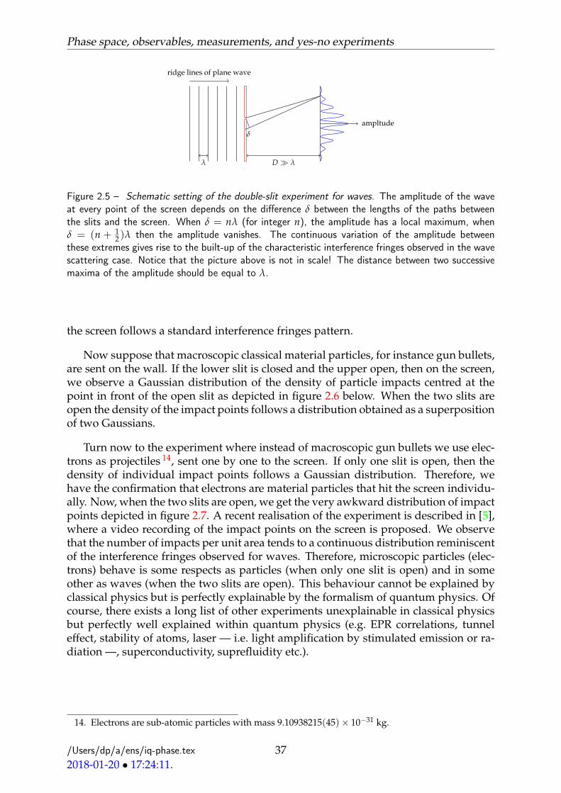
Phase space, observables, measurements, and yes-no experiments
λ
ridge lines of plane wave
D λ
ampltudeδ
Figure 2.5 – Schematic setting of the double-slit experiment for waves. The amplitude of the waveat every point of the screen depends on the difference δ between the lengths of the paths betweenthe slits and the screen. When δ = nλ (for integer n), the amplitude has a local maximum, whenδ = (n + 1
2 )λ then the amplitude vanishes. The continuous variation of the amplitude betweenthese extremes gives rise to the built-up of the characteristic interference fringes observed in the wavescattering case. Notice that the picture above is not in scale! The distance between two successivemaxima of the amplitude should be equal to λ.
the screen follows a standard interference fringes pattern.
Now suppose that macroscopic classical material particles, for instance gun bullets,are sent on the wall. If the lower slit is closed and the upper open, then on the screen,we observe a Gaussian distribution of the density of particle impacts centred at thepoint in front of the open slit as depicted in figure 2.6 below. When the two slits areopen the density of the impact points follows a distribution obtained as a superpositionof two Gaussians.
Turn now to the experiment where instead of macroscopic gun bullets we use elec-trons as projectiles 14, sent one by one to the screen. If only one slit is open, then thedensity of individual impact points follows a Gaussian distribution. Therefore, wehave the confirmation that electrons are material particles that hit the screen individu-ally. Now, when the two slits are open, we get the very awkward distribution of impactpoints depicted in figure 2.7. A recent realisation of the experiment is described in [5],where a video recording of the impact points on the screen is proposed. We observethat the number of impacts per unit area tends to a continuous distribution reminiscentof the interference fringes observed for waves. Therefore, microscopic particles (elec-trons) behave is some respects as particles (when only one slit is open) and in someother as waves (when the two slits are open). This behaviour cannot be explained byclassical physics but is perfectly explainable by the formalism of quantum physics. Ofcourse, there exists a long list of other experiments unexplainable in classical physicsbut perfectly well explained within quantum physics (e.g. EPR correlations, tunneleffect, stability of atoms, laser — i.e. light amplification by stimulated emission or ra-diation —, superconductivity, suprefluidity etc.).
14. Electrons are sub-atomic particles with mass 9.10938215(45)× 10−31 kg.
/Users/dp/a/ens/iq-phase.tex2018-01-20 • 17:24:11.
37

2.4. Classical physics does not suffice to describe Nature!
lower slit closed d = 4 d = 3 d = 2 d = 1
Figure 2.6 – Schematic setting of the double-slit experiment for gun bullets. When only the upper slitis open, we observe a Gaussian distribution of the density of impact points on the screen, centred infront of the upper slit. When the two slits are open, the density of impact points follows a distributionobtained as the superposition of two Gaussians centred in front of the slits. Depending on the distanceamong the slits the superposition can appear as unimodal or bimodal. In the above figure, the distanced among slits is given in ad hoc units (mutiples of the standard deviation of the Gaussian).
Figure 2.7 – Experimental observation of the impact points left on the screen by electrons in a doubleslit experiment. The four pictures a) – d) correspond at different instants of the experimental process.Picture a) corresponds to an early snapshot having accumulated only 11 impacts of individual electronson the screen, picture b) has 200, c) has 600, and d) has 40000. Continuing the accumulation ofimpact points, we get a continuous density of impacts that follows a pattern of interference fringes asis classically the case for waves! Source of pictures: Wikipedia, distributed under Creative CommonsLicence BY-SA 3.0.
/Users/dp/a/ens/iq-phase.tex2018-01-20 • 17:24:11.
38

Phase space, observables, measurements, and yes-no experiments
2.5 Classical probability does not suffice to describe Na-ture!
The previous section gave an example of experiment not explicable in terms of clas-sical physics. Since classical physics can be formulated as a classical probability the-ory augmented by a dynamical law, it is not surprising that classical probability turnsout to be not sufficient to explain Nature. So, the careful reader may wonder why toinclude the present section. The reason is that in the historical development of quan-tum mechanics, the statement about insufficiency of probability theory turned out tobe more controversial than the experimental evidence of the insufficiency of classicalphysics!
Quantum mechanics has been proposed as a theory explaining physical phenom-ena occurring mainly in microscopic systems. Nowadays quantum mechanics pro-vides us with a formalism that has been successfully tested in all known experimentalsituations; not a single prediction made by quantum theory has ever been falsified byan experiment! Nevertheless, the quantum formalism remains highly counter-intuitiveand several physicists have advocated the hypothesis that the theory is incomplete.The most prominent among those physicists was Einstein who refused to admit 15
the intrinsically stochastic nature of quantum mechanics in an influential paper [32]written jointly with Podolsky and Rosen in 1935, based on a Gedankenexperiment andknown as the EPR paradox 16.
When dealing with physical theories, we are confronted with two basic notions,locality and realism. Locality means that we can always take actions that have con-sequences only within a small region of space. In physics, locality stems from thefiniteness of the speed of light. Since no interaction can propagate faster than light,no influence can be sensed in space points lying beyond the wave front of light. Re-alism means that although experiments have always random outputs, the observedrandomness is nothing else than the reflection of the imperfection of the measuringinstruments. In a theory where realism applies, there is no conceptual obstruction tothink that there exists a state in which the system can be perfectly described in prin-ciple. The observed randomness is only a reflection of our incomplete knowledge ofthe precise state of the system. As we shall see later, when the standard formalism ofquantum mechanics will be introduced, this is not any longer the case for quantumsystems: quantum systems exhibit an irreducible randomness, a randomness that cannotbe removed by better describing the state. The role of the EPR paradox was to showthe incompleteness of the quantum theory. As the authors put it:
15. Cf. for instance his famous aphorism “God does not play dice with the world” (quoted from theconversations with Hermanns, in William Hermanns, Einstein and the Poet: in search of the cosmic man,Branden Press, Brookline, MA (1983).
16. See the “Analyse” item at http://bibnum.education.fr/physique/physique-quantique/le-paradoxe-epr for the unconventional beginnings and fate of the EPR paper.
/Users/dp/a/ens/iq-phase.tex2018-01-20 • 17:24:11.
39

2.5. Classical probability does not suffice to describe Nature!
“From this follows that either (1) the quantum mechanical description ofreality given by the wave function is not complete or (2) when the operatorscorresponding to two physical quantities do not commute the two quantitiescannot have simultaneous reality. For if both of them had simultaneousreality — and thus definite values — these values would enter into thecomplete description, according to the condition of completeness. If thenthe wave function provided such a complete description of reality, it wouldcontain these values; these would then be predictable. This not being thecase, we are left with the alternatives stated.”
This paper triggered extremely fruitful (although sometimes epic) discussions betweenthe tenants and the opponents of quantum formalism. Schrödinger, in a letter (inGerman) addressed to Einstein on 7 June 1935, uses for the first time the term Ver-schränkung; he translates it into entanglement 17 in the two papers he published [70, 71]to give a quantum explanation of “the EPR paradox”. In [70], Schrödinger realised thatentanglement refutes any paradoxical aspect of the EPR correlations. He has been ledto consider entanglement as the distinctive future of quantum mechanics. In his ownwords:
“When two systems (. . . ) enter into temporary physical interaction (. . . )and when after a time of mutual influence the systems separate again,then they can no longer be described in the same way as before, viz. byendowing each of them with a representative of its own. I would not callthat one but rather the characteristic trait of quantum mechanics,the one that enforces its entire departure from classical lines ofthought. By the interaction the two representatives have becomeentangled.”
Based on Einstein’s refutations, Bohm proposed, in [21, 22], a formalism of quan-tum mechanics postulating the existence of “hidden variables” (i.e. non observed ones),allowing to describe the same phenomenology as quantum mechanics without postu-lating an intrinsically stochastic nature of the theory. Therefore, the hidden variablesformalism intended to restore the realism of quantum mechanics. The introductionof hidden variables did not predict any new phenomenon beyond those predicted bystandard quantum theory and for many years, it was the root of a mainly philosophi-cal controversy between the tenants of standard quantum theory (the only one we shallpresent in the sequel of this course) and the tenants of the hidden variables description.
A major conceptual step was performed by Bell who established in [15] (see also[14]) that if hidden variables existed then they should have predictable consequencesthat could be experimentally tested. In spite of the fundamental interest such an ex-periment would have in the conceptual foundations of the theory, during several yearsit was dismissed by the scientific establishment — in another outburst of arrogance— as an uninteresting philosophical quest not worth the efforts of respectable scien-tists 18. Due to the enormous success of quantum mechanics to quantitatively predict
17. This notion will be defined in §4.4.18. Readers so inclined to philosophical meditation are invited to consider the ravages “fashion-led”
or “project-oriented” research can cause to the advancement of science.
/Users/dp/a/ens/iq-phase.tex2018-01-20 • 17:24:11.
40

Phase space, observables, measurements, and yes-no experiments
all observed phenomena, a utilitarian attitude condensed into the motto “shut up andcompute” prevailed in the scientific circles. It was only thanks to the ingeniousness ofseveral groups of experimental physicists around the world (Clauser, Shimony, Horne,Holt, Aspect, Dalibard, Roger who persevered in willing to experimentally test the hy-pothesis of hidden variables) that the existence of both local and realistic physical the-ories has been refuted in the three seminal papers [7, 8, 6] of the group at the Universitéd’Orsay. This experiment, of the utmost fundamental importance, is described in para-graph 2.5.2. It establishes that a theory that is simultaneously local and realistic cannotreproduce all the predictions of quantum mechanics (hence cannot explain experimen-tal observations either). Phrased differently, assuming realism, the phenomenon ob-served in this experience — when interpreted within classical probability — appearsas non-local. This fact is sometimes wrongly termed quantum non-locality in the liter-ature. This term will never be used in the sequel of this course.
Therefore, before presenting the nowadays accepted form of quantum mechanics,we spend some lines to describe Bell’s inequalities and explain in some details the Or-say experiment (see §2.5.2 below). We follow the exposition of [51] to refute the hiddenvariables hypothesis. The quantum mechanical explanation of the Orsay experiment— postponed after the introduction of the quantum formalism — will be given in §4.5.
2.5.1 Bell’s inequalities
Proposition 2.5.1 (The three-variable Bell’s inequality). Let X1, X2, X3 be an arbitrarytriple of 0, 1-valued random variables defined on some probability space (Ω,F , P). Then
P(X1 = 1, X3 = 0) ≤ P(X1 = 1, X2 = 0) + P(X2 = 1, X3 = 0).
Proof:
P(X1 = 1, X3 = 0) = P(X1 = 1, X2 = 0, X3 = 0) + P(X1 = 1, X2 = 1, X3 = 0)≤ P(X1 = 1, X2 = 0) + P(X2 = 1, X3 = 0).
Proposition 2.5.2 (The four-variable Bell’s inequality). Let X1, X2, Y1, Y2 be an arbitraryquadruple of 0, 1-valued random variables defined on some probability space (Ω,F , P).Then
P(X1 = Y1) ≤ P(X1 = Y2) + P(X2 = Y2) + P(X2 = Y1).
Proof: The random variables being 0, 1-valued, it is enough to check on all 16 possiblerealisations of the quadruple (X1(ω), X2(ω), Y1(ω), Y2(ω)) that
X1 = Y1 ⊆ [X1 = Y2] ∨ [X2 = Y2] ∨ [X2 = Y1].
/Users/dp/a/ens/iq-phase.tex2018-01-20 • 17:24:11.
41

2.5. Classical probability does not suffice to describe Nature!
α β
Figure 2.8 – When a photon passes through the first polariser — oriented in direction α — emergespolarised in that direction. When it encounters a second polariser — oriented in direction β — passesthrough with probability cos2(α− β). If the photon is initially already polarised in direction α, nothingchanges if the first polariser is removed.
2.5.2 The Orsay experiment(s)
The idea behind what is called nowadays “the Orsay experiment” 19 is to associateprecise physical observables with the 0, 1-valued quantities occurring in Bell’s in-equalities. Classical theory describes light as an electromagnetic wave; the electric fieldoscillates in a plane perpendicular to the propagation direction known as polarisation.(Some additional details on the nature and properties of light are given in appendix A).When monochromatic light emitted from a random source (i.e. unpolarised) of someintensity I passes through a polariser, the emerging beam is polarised in the directionof the polariser and has intensity I/2. Now, it has been established that a light beam iscomposed of a great number of elementary light quanta called photons
Therefore, the statement on intensities made above have only a statistical mean-ing; if a photon passing through a polariser (oriented in a given direction α) encoun-ters a second polariser oriented (in a direction β) has probability 1
2 cos2(α− β) to passthrough (see figure 5.1). This is an experimental fact, in accordance with both quantummechanical prescriptions and with classical electromagnetic theory of light.
If the experiment is to be explained in terms of classical probability, with everypolariser in direction α ∈ [0, π/2] is associated a random variable Xα ∈ 0, 1; therandom variables X are defined on a probability spaces (Ω,F , P) where ω ∈ Ω repre-sent the microscopic state of the photon. Now for the experimental setting depicted infigure 5.1, the random variables X are correlated as
E(XαXβ) = P(Xα = 1, Xβ = 1) =12
cos2(α− β).
But now there is a problem because this correlation cannot be that of classical randomvariables. Choosing in fact three polarisations α1, α2, and α3, we have P(Xαi = 1, Xαj =
0) = P(Xαi = 1)− P(Xαi = 1, Xαj = 1) = 12(1− cos2(αi − αj)) = 1
2 sin2(αi − αj) fori, j ∈ 1, 2, 3. The three-variable Bell inequality 2.5.1 reads then
12
sin2(α1 − α3) ≤12
sin2(α1 − α2) +12
sin2(α2 − α3).
19. As a matter of there has been two experiments.
/Users/dp/a/ens/iq-phase.tex2018-01-20 • 17:24:11.
42

Phase space, observables, measurements, and yes-no experiments
αi
PM1
Coincidence monitoring
PM2
β j
Ca
Figure 2.9 – Schematic view of the Orsay experiment [8]. A beam of calcium (Ca) atoms is triggeredby a laser. When thus excited, a calcium atom emits simultaneously two photons (at differentfrequencies) in opposite directions and having correlated polarisations. Two polarisers stand to theleft and to the right the calcium beam, at equal optical distances from it. An ingenious system of rapidoptical switches is used whose net effect can be described by the following equivalent description.After the two photons have been emitted, the left polariser is oriented according to an angle randomlychosen in the set α1, α2, the right polariser according to an angle randomly chosen in the setβ1, β2. The optical distance between the beam and the polarisers is sufficiently large to allowenough time for the switching to take place after the emission of the photons and before theirreaching the polarisers (so that any causal influence of the choice of orientations on the manner thephotons are emitted is safely excluded). After passing through the polarisers, the photons are detectedby photomultipliers (PM1) and (PM2) and only photons in synchronisation are recorded.
The choice α1 = 0, α2 = π/6, and α3 = π/3 leads to the impossible inequality 3/8 ≤1/8 + 1/8. Therefore, classical probability cannot describe this simple experiment.
On a second reading, this experiment is not very convincing because on arrangingpolarisers on the optical table as described above, there is nothing preventing concep-tually the second random variable Xβ to depend in fact on both α and β. But then thecorrelation reads E(XαXα,β) = P(Xα = 1, Xα,β = 1) = 1
2 cos2(α− β) and this can besatisfied by choosing, for instance, Xα and Xα,β independent with P(Xα = 1) = 1/2and P(Xα,β = 1) = cos2(α− β) which of course can be easily conceived.
The irrefutable evidence of the impossibility of describing Nature with merely clas-sical probability is provided through the second experiment Aspect, Dalibard andRoger performed in 1982, [6], schematically described in figure 2.9. (Please carefullyread the caption of this figure where the precise experimental setting is described). Thesame analysis can be made as in the previous experimental setting. Denoting by Xα the0, 1-valued random variable quantifying the passage of the photon through the leftpolariser and Yβ through the right one, it is experimentally established in [6] that,
P(Xα = Yβ) =12
sin2(α− β),
for every choice of α and β. (Note incidentally that the same conclusion is obtainedusing — the not yet presented — quantum formalism). Now the choice α1 = 0, α2 =π/3, β1 = π/2, and β2 = π/6, should read 1 ≤ 1/4 + 1/4 + 1/4, manifestly violatingthe four variable Bell’s inequality 2.5.2.
To better grasp the significance of this experiment, it has been proposed, see [51] for
/Users/dp/a/ens/iq-phase.tex2018-01-20 • 17:24:11.
43

2.5. Classical probability does not suffice to describe Nature!
instance, to think of it as a card game between two players X and Y who can pre-agreeon any conceivable strategy in order to win the game. The game is described in thefollowing
Exercise 2.5.3. (The Orsay experiment as a card game [51]) The game is played be-tween players X, Y (see figure 2.9), and A (like . . . Aspect) who acts as an arbiter andas game leader.
Description of the game
— A disposes of a well shuffled deck of red and black cards (consider it as aninfinite sequence of i.i.d. red, black-valued random variables uniformly dis-tributed on red, black := r, b).
— X and Y are free to use random resources (e.g. dice) if they wish.— Before the game starts, X and Y agree on given strategy (deterministic, non-
deterministic, or random) how to determine a yes, no-valued variable out ofthe colour of the card they will be presented. Once the game starts, the playersare not allowed any longer to communicate.
— A picks two cards from the deck and presents the one to X and the other to Y(mind that X and Y don’t know each other’s card).
— X and Y apply their own pre-agreed strategy to the colour they are presentedand simultaneously say yes or no.
— After the announcement of the players, the cards are laid on the table. Fourdifferent card pairs are possible (rr), (rb), (br), (bb), where the first colour refersto the colour of the X’s card and the second to the Y’s one (consider these colourpairs as boxes in a 2× 2 board). If both players have given the same answerthen 1 is written in the corresponding box, else 0 is marked.
— In the course of the game, the boxes get filled by sequences of 0’s and 1’s.— Let πcc′ , with c, c′ ∈ r, b, be the limit of the empirical probability of 1’s in the
box corresponding to colours (cc′) when the game runs indefinitely. The playerswin the game if πrr > πrb + πbr + πbb. The purpose is to show that there existsno strategy (deterministic or random) allowing the players to win the game.
Questions
1. Suppose that X and Y have agreed on the following strategy: X always says“yes”, independently of the colour of the card presented to her/him and Y an-swers the question “is my card red?”. Compute explicitly the values of πcc′ forc, c′ ∈ r, b and show that with this deterministic strategy, the numbers πcc′
satisfy the four variable Bell’s inequality πrr ≤ πrb + πbr + πbb.2. In the above strategy, the decision making process is described through the ma-
trices DX and DY with DX : r, b × 0, 1 → [0, 1] (and similarly for DY), de-fined respectively by
DX =
(0 10 1
)and DY =
(0 11 0
),
interpreted as meaning P(Answer of X is a | card colour is c) = DX(c, a) forc ∈ r, b and a ∈ 0, 1 (and similarly for Y). Hence the previously described
/Users/dp/a/ens/iq-phase.tex2018-01-20 • 17:24:11.
44

Phase space, observables, measurements, and yes-no experiments
strategies are termed deterministic strategies. There are 4 deterministic strate-gies for every player. Determine all 16 pairs of deterministic strategies and showthat for all of them, Bell’s inequality is verified.
3. Propose a plausible parametrisation of the space of all strategies (deterministicand random) and show that this space is convex. Is it a simplex? Show that theprevious deterministic strategies are extremal points of this space.
4. Conclude that in general any strategy can be written as a convex combinationof deterministic strategies. Is this decomposition unique? How such a convexcombination is related to hidden variables? Conclude that no classical strategyexists allowing to win this game.
Some hints concerning convexity and convex decomposition of stochastic matricesneeded for the the two last questions can be found in the chapter “Markov chainson finite state spaces” of the lecture notes [60].
This exercise shows that any system described in terms of classical probabilities,even augmented to incorporate hidden variables, cannot win this game. But the Orsayexperiment proved that Nature wins! Therefore, the quantum strategy used by Natureis strictly more powerful than any classical strategy. Probably the first person to reallyunderstand this power was Feynman (see [39, chap. 7 and 15] for instance), who firstconjectured the computational power of quantum mechanics and was the first whoproposed to use atoms as quantum computers.
Nowadays, many other experiments have been performed to refute the hiddenvariables hypothesis. We shall present in §4.6 the most recent one based on the vio-lation of Bell’s test in the form of the so called CHSH inequalities.
2.6 Quantum systems (elementary formulation)
Quantum mechanics emerged thanks to various experimental and theoretical ad-vances, due mainly to Bohr, Planck, Schrödinger, Heisenberg, Dirac, and many oth-ers. Various formulations of quantum mechanics are possible. We start from themost straightforward one [84], based on the Hilbert space formalism, introduced byvon Neumann in 1932. It turns out that shortly after the publication of this text, vonNeumann confessed that he was not satisfied with the Hilbert space formulation ofquantum mechanics (see [63] for a review of the ideas of von Neumann on quantummechanics that pays due attention to historical facts). Later on, a more general for-mulation [81], based on quantum logics and C∗-algebras, will be given; this formula-tion has the advantage of allowing a unified treatment for both classical and quantumsystems. Another possible formulation is provided by the operational formulation ofquantum mechanics, based on the notion of instrument (see [30, 56, 58, 59]) or infor-mational formulation (see [27, 28] for instance). The reader may wonder why so manyformulations have been proposed so far. The answer is that although all the formu-lations are totally satisfactory from the computational point of view, their predictivepower, and their adaptedness to explain diverse experiments, none of the existingones is philosophically and epistemologically satisfactory. Quantum mechanics is a
/Users/dp/a/ens/iq-phase.tex2018-01-20 • 17:24:11.
45

2.6. Quantum systems (elementary formulation)
partial theory, describing fragile systems, i.e. systems that eventually leave the quan-tum realm to enter the classical one; such a fragility demands for a unified treatmentof classical and quantum formalism, not guaranteed by any of the existing formalisms.The most counter-intuitive postulate of quantum mechanics is the measurement postu-late that obsessively tormented physicists since the early days of quantum mechanics(see [78, 76, 77] or [11] for a critical account of the previous references).
2.6.1 Postulates of quantum mechanics (sharp effects and pure states)
For the time being, we proclaim that a quantum system verifies the following pos-tulates, given in the same order as the postulates for classical systems. These postulateshold for very simple quantum systems (mainly for systems with finite degrees of free-dom with non-degenerate observables). They will be completed and extended later tocover more complicated systems.
Postulate 2.6.1 (Phase space). The phase space of a quantum mechanical system is a separablecomplex Hilbert space H. Events are associated with Hilbert subspaces of H. When twosystems, respectively described by Hilbert spaces H1 and H2, are considered as a single system,the composite system is described by the Hilbert space H1 ⊗H2 where ⊗ denotes the tensorproduct.
Postulate 2.6.2 (States). Unit vectors 20 of H correspond to pure 21 quantum states Sp.More precisely, with a unit vector ψ, we associate the spanned one-dimensional Hilbert sub-space Cψ and we denote by ρ = ρψ the orthoprojection onto Cψ. The set of pure states is thenidentified with Sp = ρψ, ψ ∈H, ‖ψ‖ = 1 ' Cψ.
Postulate 2.6.3 (Evolution). Any time evolution of an isolated quantum system is describedby a unitary operator acting on H. Conversely, any unitary operator acting on H correspondsto a possible invariance 22 of the system.
Postulate 2.6.4 (Observables). The set Os of sharp observables of a quantum system is theset of bounded self-adjoint operators X acting on the phase space H of the system. The space ofoutcomes of a sharp observable X is its spectrum, i.e. X = spec(X). Sharp effects E[A] arespecial self-adjoint operators occurring as spectral projections of an observable. The set of sharpeffects is denoted by Es. Conversely, if a projective resolution of unity E : B(R) → B(H) isgiven, we can associate the self-adjoint operator X having E as spectral projections. The set ofeffects (unsharp or fuzzy ones) E is the convex hull of Es.
Postulate 2.6.5 (Measurement). Measuring a sharp observable represented by its spectralprojectors (effects) E, in the pure state ρψ described by the unit vector ψ, corresponds to deter-mining the possible outcomes and the probability measure ν
ρψ
E on the real line induced by thespectral projectors through the formula
νρψ
E (B) = tr(ρψE[B]) = 〈ψ | E[B]ψ 〉, ∀B ∈ B(R) = tr(ρψE[B]) = 〈ρψ, E[B]〉,
20. Strictly speaking, equivalence classes of unit vectors differing by a global phase, called rays. Forthe sake of simplicity we stick to unit vectors in this introductory section.
21. The structure of the set of arbitrary states is postponed to postulate 3.11.8 that generalises thepresent one.
22. The time evolution of an isolated system leaves the physical quantity “energy” invariant. Unitaryoperators are associated with conserved quantities. See definition 12.5.4 and the reformulation of thepresent postulate as postulate 12.5.5 for precise statements.
/Users/dp/a/ens/iq-phase.tex2018-01-20 • 17:24:11.
46

Phase space, observables, measurements, and yes-no experiments
where 〈·, ·〉 denotes the duality bracket on Sp ×Os
2.6.2 Interpretation of the basic postulates
These postulates will be revisited later, after some basic notions on Hilbert spaceshave been reminded. For the time being, it is instructing to illustrate the implicationsof these axioms on a very simple non-trivial quantum system and interpret their sig-nificance. Beyond its pedagogical interest, this simple example has also an intrinsicinterest since it describes any physical system with two internal degrees of freedomserving to model a qubit, the quantum analog of a bit.
Phase space. We study a quantum system whose phase space H = C2. This is thesimplest non-trivial situation that might occur and could describe, for instance,the internal degrees of freedom of an atom having two states. In spite of itsapparent simplicity, the systems carries already very interesting features. Noticehowever that in general, even for very simple finite systems, the phase space isnot necessarily finite-dimensional.Every f ∈ H can be decomposed into the canonical basis (ε1, ε2) as f = f1ε1 +f2ε2 with f1, f2 ∈ C. If ‖ f ‖ 6= 0, denote by φ = f /‖ f ‖ the correspondingnormalised vector 23.
(Pure) states. Now φ = φ1ε1 + φ2ε2 with |φ1|2 + |φ2|2 = 1 corresponds to a purestate. The numbers |φ1|2 and |φ2|2 are non-negative reals summing up to 1;therefore, they are interpreted as a probability on the finite set of coordinates1, 2. Consequently, the complex numbers φ1 = 〈 ε1 | φ 〉 and φ2 = 〈 ε2 | φ 〉 arecomplex probability amplitudes, their squared moduli represent the probabilitythat a system in a pure state φ is in the pure state ε1 or ε2.Notice that pure states can be written as linear superpositions φ = φ1ε1 + φ2ε2meaning that a pure state φ can have components in two other pure states ε1and ε2. But this does not mean that the pure state φ can be written as a convexcombination of the pure states ε1 and ε2. The complex numbers φ1 and φ2 haveno probabilistic interpretation; only their squared amplitudes have.
Evolution. A unitary operator on H is a 2× 2 matrix U, verifying UU∗ = U∗U =I. If φ is a pure state, then ψ = Uφ verifies ‖ψ‖2 = 〈Uφ |Uφ 〉 = 〈 φ |U∗Uφ 〉 =‖φ‖2. Therefore quantum evolution transforms pure states into pure states (pre-serves purity of states). Moreover, due to the unitarity of U, we have φ = U∗ψ,and since U∗ is again unitary, it corresponds to a possible time evolution (as amatter of fact to the time reversed evolution of the one corresponding to U.)This shows that time evolution of isolated quantum systems is reversible.
(Sharp) effects and observables. Recall that any normal operator X admits a spec-tral decomposition X =
∫spec(X) E[dx]x. If X is self-adjoint, then spec(X) ⊆ R.
Let us illustrate with a very simple example: chose for X the matrix
X =
(1 2i−2i −2
).
23. General (unnormalised) vectors of H are denoted by small Latin letters f , g, h, etc.; normalisedvectors, representing rays, by small Greek letters φ, χ, ψ, etc.
/Users/dp/a/ens/iq-phase.tex2018-01-20 • 17:24:11.
47

2.6. Quantum systems (elementary formulation)
We compute easilyEigenvalues Eigenvectors Projectors
x ζ[x] E[x]
−3 1√5
(−i2
)15
(1 −2i2i 4
)2 1√
5
(2i1
)15
(4 2i−2i 1
)Hence
X = ∑x∈−3,2
E[x]x = (−3)15
(1 −2i2i 4
)+ 2
15
(4 2i−2i 1
).
Since the operator X is self-adjoint (hence normal), eigenvectors associated withdifferent eigenvalues are orthogonal (see §3.7, corollary ??). The operators E[−3]and E[2] are self-adjoint (hence they correspond to observables) and othoprojec-tors to mutually orthogonal subspaces. Since their spectrum is 0, 1, they playthe role of yes-no questions for a quantum system.
Measurement. This axiom in some respects generalises straightforwardly the clas-sical case; in some other it has the most counter-intuitive consequences.Straightforward generalisation of classical case: Let ψ ∈ H be a pure phase; since
ζ[−3] and ζ[2] are two orthonormal vectors of H (hence also pure phases),they serve as basis to decompose ψ = z−3ζ[−3]+ z2ζ[2], with ‖ψ‖2 = |z−3|2 +|z2|2 = 1. Thus any pure state ψ, with probability |〈ψ | ζ[−3] 〉|2 is in the purestate ζ[−3] and with probability |〈ψ | ζ[2] 〉|2 is in the pure state ζ[2].Compute further
νρψ
X (x) = tr(ρψE[x]) = 〈ψ | E[x]ψ 〉= ∑
x′ ,x′′∈spec(X)
zx′zx′′〈 ζ[x′] | E[x]ζ[x′′] 〉 = |zx|2 ∈ [0, 1].
Thus (|zx|2)x∈spec(X) can be interpreted as a probability on the set of the spec-tral values. Hence, the scalar product 〈ψ |Xψ 〉 = ∑x∈spec(X) x|zx|2 is the ex-pectation of the spectral values with respect to the decomposition of ψ on thebasis of eigenvectors. It is worth noticing that expectation of a classical ran-dom variable X taking values in a finite set x1, . . . , xn with probabilitiesp1, . . . , pn respectively, is
EX =n
∑k=1
xk pk =n
∑k=1
√pkxk√
pk =n
∑k=1
√pk exp(−iθk)xk
√pk exp(iθk),
with arbitrary θk ∈ R, k = 1, . . . , n. Hence, classically, EX = 〈ψ |Xψ 〉 with
ψ =
√
p1 exp(iθ1)...√
pn exp(iθn)
, verifying ‖ψ‖ = 1 and with X =
x1 0. . .
0 xn
.
We have moreover seen that classical probability is equivalent to classicalphysics; thanks to the previous lines, it turns out that it is also equivalentto quantum physics involving solely diagonal self-adjoint operators as ob-servables. The full flavour of quantum physics is obtained only when theobservables are represented by non-diagonal self-adjoint operators.
/Users/dp/a/ens/iq-phase.tex2018-01-20 • 17:24:11.
48

Phase space, observables, measurements, and yes-no experiments
Counter-intuitive consequences: Consider now,
f [x] = E[x]ψ =
〈 ζ[x] |ψ 〉ζ[x] if x ∈ spec(X)0 otherwise.
The vector f [x] is in general unnormalised; the corresponding normalisedstate φ[x] = E[x]ψ
‖E[x]ψ‖ , well defined whenever x ∈ spec(X) and ψ has a non-zero ζ[x]-component, has a very particular interpretation. Suppose we askthe question: “does the physical observable take the value−3?” The answer,as in the classical case, is a probabilistic one:
P(X = −3) = νρψ
X (−3) = |z−3|2 = 〈 f [−3] | f [−3] 〉 = ‖E[−3]ψ‖2 = tr(ρψE[−3]).
What is new, is that once we have asked this question, the state ψ is projectedon the eigenspace E[−3]H and is represented by the state φ[−3]. This meansthat asking a question on the system has irreversibly changed its state! Theconditional state ρφ[x] given that we have asked the question E[x] reads now
ρφ[x] =E[x]ρψE[x]tr(ρψE[x])
.
But now, the state has been irreversibly modified. If we apply the total prob-ability formula, we obtain
∑x∈spec(X)
ρφ[x] tr(ρψE[x]) = ∑x∈spec(X)
E[x]ρψE[x] 6= ρψ,
due to the non-commutativity of ρψ and E[x]. This is a totally new phe-nomenon without classical counterpart. Asking questions about a quan-tum system corresponds to a quantum measurement and the above formulashows that measurement irreversibly changes (projects) the state of the sys-tem. It will be shown later that the above averaging over the possible out-comes of a sharp observable X irreversibly transforms the quantum state ρψ
into the state ∑x∈spec(X) E[x]ρψE[x] that is isomorphic to a classical state.
Example 2.6.6. (A quantum Gedankenexperiment). Suppose that a a huge number, N,of copies of a “quantum die” has been prepared in a quantum state ρ guaranteed togive output x with probability tr(E[x]ρ) and repeat the experiment as described in theclassical setting of the example 2.3.25. Then of course, N[x]/N will tend to tr(E[x]ρ)as was the case in the classical situation. But now it follows from the formalism andis experimentally verified that N[xx]/N[x] → 1! This is a totally new phenomenon,without classical counterpart. It is termed collapse of the quantum state after a sharpmeasurement.
There are many other counter-intuitive quantum phenomena; we shall study someof them in this course.
Summarising the interpretation of these axioms, we have learnt that— quantum mechanics has a probabilistic interpretation, generalising the classical
probability theory to a quantum (non-Abelian) one,
/Users/dp/a/ens/iq-phase.tex2018-01-20 • 17:24:11.
49

2.6. Quantum systems (elementary formulation)
— quantum evolution is reversible (as is the classical one),— quantum measurement is irreversible and this constitutes a highly counter-intuitive
aspect of quantum mechanics.Were only to consider this generalisation of probability theory to a non-commutative
setting and to explore its implications for explaining quantum physical phenomena,should the enterprise be already a fascinating one. But there is even much more fas-cination about it: there has been demonstrated lately that quantum phenomena canserve to cipher messages in an unbreakable way and these theoretical predictions havealready been exemplified by currently working pre-industrial prototypes 24.
In a more speculative perspective, it is even thought that in the near future therewill be manufactured computers capable of performing large scale computations us-ing quantum algorithms 25. Should such a construction be realised, a vast family ofproblems in the (classical) complexity class of “exponential time” could be solved inpolynomial time on a quantum computer.
24. See the article [35], articles in Le Monde (they can be found on the website of this course), thewebsite www.idquantique.com of the company commercialising quantum cryptologic and teleportingdevices, etc.
25. Contrary to the quantum transmitters and cryptologic devices that are already available (withinpre-industrial technologies), the prototypes of quantum computers that have been manufactured so farhave still extremely limited scale capabilities.
/Users/dp/a/ens/iq-phase.tex2018-01-20 • 17:24:11.
50

3Short resumé of Hilbert spaces
For the sake of completeness, some standard results on Hilbert spaces are remindedin this chapter. Most of the proofs in this chapter are omitted because they are consid-ered as exercises; they can be found in the classical textbooks [3, 40, 64, 67, 87] whichare strongly recommended for further reading.
This chapter is written with two different readerships in mind: those interestedsolely in finite dimensional applications of quantum mechanics and those interested infull-fledged applications. The former can skip the passages printed in colour.
3.1 Scalar products and Hilbert spaces
Hilbert spaces have many distinct features. They are C-vector spaces (hence arealgebraic objects) equipped with a Hermitean scalar product (hence angles and ge-ometry follow) from which a Hilbert norm can be defined (they thus become analyticobjects) for which they are complete (hence a unit vector ψ has components on an or-thonormal basis (en) reading ∑n |ψn|2 = 1; therefore its components can be interpretedas probability amplitudes).
Definition 3.1.1. Let V be a C-vector space, u, v, w ∈ V, and α, β ∈ C. A form s :V×V→ C is
— sesquilinear it it is— linear with respect to the second 1 argument: s(u, αv + βw) = αs(u, v) +
βs(u, w), and
1. Notice that very often in the literature, the scalar product is defined to be linear with respect to itsfirst argument. This is only a matter of taste that must be consistently kept in the whole formalism. Westick in the definition given here because it greatly simplifies formulæ arising in the quantum mechanicalsetting.
51

3.1. Scalar products and Hilbert spaces
— antilinear with respect to first argument: s(αu+ βv, w) = αs(u, w)+ βs(v, w);— Hermitean if it sesquilinear and s(u, v) = s(v, u),— positive: s(v, v) ≥ 0, and— definite: s(v, v) = 0⇔ v = 0.
A Hermitean positive definite form is a a scalar product. The scalar product s is de-noted usually 〈 · | · 〉 and the pair (V, 〈 · | · 〉) is called a pre-Hilbert space. Two vectorsv and w are called orthogonal if 〈 v |w 〉 = 0.
Lemma 3.1.2. Let (V, 〈 · | · 〉) be a pre-Hilbert space and u, v ∈ V. The following hold:— Buniakowski-Cauchy-Schwarz inequality: |〈 u | v 〉| ≤
√〈 u | u 〉
√〈 v | v 〉,
— The scalar product defines uniquely a norm ‖v‖ =√〈 v | v 〉, called the Hilbert norm;
the scalar product is recovered from the Hilbert norm through the polarisation equal-ity
〈 u | v 〉 = 14
3
∑k=0
(−i)k‖u + ikv‖2.
— The function 〈 · | · 〉 : V×V→ C (hence the norm) is continuous.— The parallelogram rule holds, i.e.
‖u− v‖2 + ‖u + v‖2 = 2‖u‖2 + 2‖v‖2.
Lemma 3.1.3. [85, Th. 1.6, p. 9]: Let (V, ‖ · ‖) be a normed space. The norm is stemmingfrom a scalar product on V if, and only if, the norm satisfies the parallelogram rule.
Exercise 3.1.4. Give a Hilbert proof of Pythagoras theorem.
As stated above, the scalar product of a pre-Hilbert space (V, 〈 · | · 〉) induces aHilbert norm ‖v‖ =
√〈 v | v 〉 turning (V, ‖ · ‖) into a normed space; furthermore,
the Hilbert norm defines a distance d(x, y) = ‖x− y‖, turning thus (V, d) into a metricspace. We can therefore define the notion of a fundamental (Cauchy) sequence on V
as being a sequence v = (vn)n∈N of vectors vn ∈ V such that for every ε > 0 thereexists N = N(ε) ∈ N such that for m, n ≥ N, we have d(vn, vm) < ε. Nevertheless,nothing imposes that any fundamental sequence converges within V. If such is thecase, the metric space (V, d) (or the normed space (V, ‖ · ‖) is termed complete or Ba-nach space. A pre-Hilbert space that is complete for the metric induced by its Hilbertnorm is called a Hilbert space. A subset A ⊂ V of a Banach space is termed closed ifit contains the limits of all Cauchy sequences constructed from elements of A.
Usually we use the symbols F, G, H to denote Hilbert spaces instead of the genericsymbol U, V, W, X, Y, used for arbitrary spaces, i.e. when no further precision isgiven, F, G, H will stand for Hilbert spaces. In the same vein, vectors of a Hilbertspace are usually denoted by e, f , g, h, etc. or ε, ζ , η, φ, ψ, etc. instead of the genericnotation u, v, w, x, y, z, etc. for vectors in an arbitrary vector space.
Definition 3.1.5. Let (V, ‖ · ‖) be a normed space and A ⊂ V. The linear span of A,denoted vect(A), is the intersection of all subspaces of V which contain A; the closedlinear span of A, denoted vect(A), is the intersection of all closed subspaces of V whichcontain A.
/Users/dp/a/ens/iq-hilbe.tex2018-01-18 • 10:54:05.
52

Short resumé of Hilbert spaces
We recall that a complete metric space (V, d) is called a completion of a metricspace (V, d) if there exists an isometric embedding ι : V → V such that the imageι(V) is dense in V. An arbitrary normed space (not necessarily complete) can be com-pleted via a standard procedure we recall here briefly. Let CS(V) be the set of Cauchysequences on V, ∼ an equivalence relation on CS(V) defined, for sequneces v = (vn)and w = (wn), by
v ∼ w⇐⇒ limn→∞‖vn − wn‖ = 0,
and V = CS(V)/ ∼ the set of equivalence classes of ∼. The space V has a naturalvector space structure and through the definition
V 3 [v] 7→ ‖[v]‖ = limn→∞‖vn‖
— that can be shown to be independent of the representative v of [v] — becomes acomplete normed space. On identifying elements of V with constant sequences in V
we establish a canonical embedding ι : V→ V.
Theorem 3.1.6. For each normed (Hilbert) vector space V, there exists a completion V. Twoarbitrary completions (stemming from the same norm) are isomorphic.
Proof. See [40, §1.6, pp. 17–21] or [85, Th. 4.11, p. 64].
Exercise 3.1.7. The following are classical examples of normed spaces.1. The finite-dimensional vector space V = Cd with the ordinary scalar product〈 u | v 〉 = ∑d
n=1 unvn is obviously a Hilbert space.2. Let V = Md,d′(C) the set of d × d′ matrices with complex coefficients. Then〈 u | v 〉 = tr(u∗v), where u∗ denotes the transposed complex conjugate matrixof u, is a scalar product.
3. On defining ‖v‖p = (∑n∈N |vn|p)1/p for 1 ≤ p < ∞ and ‖v‖∞ = supn∈N |vn|,the spaces V = `p(N) are complete normed (Banach) spaces 2 for all 1 ≤ p ≤ ∞.The case p = 2 is very special, since `2(N) a Hilbert space with a scalar prod-uct, compatible with ‖ · ‖2, defined by 〈 u | v 〉 = ∑n∈N unvn. It is the infinite-dimensional generalisation of the example 1.
4. More generally, let A be an arbitrary set (not necessarily countable), µ : A →]0, ∞[, and p ∈ [1, ∞[. Consider functions v : A → C vanishing outside acountable set (that generally depends on v) and denote by
`p(A, µ) = v : A→ C, s.t. v ≡ 0 but on a countable set, ∑a∈A
|v(a)|pµ(a) < ∞ ⊆ CA.
On defining ‖v‖p := (∑a∈A |v(a)|pµ(a))1/p, the space `p(A, µ) becomes a normedspace. In particular, `2(A, µ) is a Hilbert space.
5. The space V = Lp([a, b], λ) with 1 ≤ p < ∞ can be equipped with a norm
‖ · ‖p defined by ‖v‖p =(∫
[a,b] |v(t)|pλ(dt)
)1/p. Then (V, ‖ · ‖p) is a Banach
space. For p = 2, it becomes also a Hilbert space for the scalar product 〈 u | v 〉 =∫[a,b] u(t)v(t)λ(dt).
2. Note that ‖v‖p = (∑n∈N |vn|p)1/p is well defined also for 0 < p < 1; nevertheless, in those cases,‖v‖p is not a norm. The spaces (`p(N), dp) with dp(v, w) = ∑n∈N |vn − wn|p are metric spaces for0 < p < 1.
/Users/dp/a/ens/iq-hilbe.tex2018-01-18 • 10:54:05.
53

3.2. Orthogonal and orthonormal systems; orthogonal complements
6. The space V = Ck([a, b]) can be equipped with a scalar product 〈 u | v 〉 =
∑kj=0∫[a,b] u(j)(t)v(j)(t)dt. The corresponding norm is denoted ‖ · ‖Wk,2 but the
normed space (V, ‖ · ‖Wk,2) is not complete. Its completion is called Sobolevspace Wk,2([a, b]) and is a Hilbert space. In particular, W0,2([a, b]) = L2([a, b]).
Recall that a subset C of a real or complex vector space V is convex if for all point(vectors) x, y ∈ C and all λ ∈ [0, 1], the point λx + (1− λ)y belongs to C.
Theorem 3.1.8. Let C be a non-empty, closed, convex set in a Hilbert space H. For anyh ∈H, there exists a unique point c ∈ C lying closer to h than any other point of C, i.e.
∀h ∈H, ∃!c := c(h) ∈ C : ‖h− c‖ = infa∈C‖h− a‖.
Corollary 3.1.9. Let G be a Hilbert subspace of H. Then, for all h ∈H, there exists a uniqueg ∈ G, such that
‖h− g‖ = inff∈G‖h− f ‖ and h− g ⊥ G.
Exercise 3.1.10 (An important one for probabilists). Let L1(Ω,F , P; C) denote the vec-tor space of integrable random variables over some probability space (Ω,F , P) and Ga sub-σ-algebra of F . Denote by F = L2(Ω,F , P; C) and G = L2(Ω, G , P; C). OnF a sesquilinear form s can be defined by s(X, Y) =
∫Ω X(ω)Y(ω)P(dω) that can be
turned into a scalar product by considering the space L2 instead of L2.1. Use corollary 3.1.9 to establish that for every X ∈ F there exists a Y ∈ G (unique
up to modifications differing from X on P-negligible sets), such that X−Y ⊥ Zfor all Z ∈ G.
2. Use the previous result, with Z = 1G for an arbitrary G ∈ G, to establish that Yis a version of the (classical) conditional expectation E(X|G).
3. Use the density of L2 into L1 and the monotone convergence theorem to estab-lish that for every random variable X ∈ L1(Ω,F , P; C), there exists a randomvariable Y ∈ L1(Ω, G , P; C) verifying
∀G ∈ G ,∫
GX(ω)P(dω) =
∫G
Y(ω)P(dω).
3.2 Orthogonal and orthonormal systems; orthogonal com-plements
Lemma 3.2.1. Let (ei)i=1,...,n be a collection of vectors of a Hilbert space H.1. If the collection are orthogonal, then ‖∑n
i=1 ei‖2 = ∑ni=1 ‖ei‖2.
2. If the collection are orthonormal, (λi)i=1,...,n are arbitrary complex numbers and h ∈H
arbitrary, then
‖h−n
∑i=1
λiei‖2 = ‖h‖2 +n
∑i=1|λi − ci|2 −
n
∑i=1|ci|2,
where ci = ci(h) := 〈 ei | h 〉.
/Users/dp/a/ens/iq-hilbe.tex2018-01-18 • 10:54:05.
54

Short resumé of Hilbert spaces
The significance of the previous result is better grasped in the following:
Theorem 3.2.2. If (ei)i=1,...,n is an orthonormal collection of vectors in H, the vector g ∈vect(e1, . . . , en) lying closest to h is the vector g = ∑n
i=1 〈 ei | h 〉ei, verifying ‖h − g‖2 =‖h‖2 −∑n
i=1 |〈 ei | h 〉|2.
In particular, if h ∈ vect(e1, . . . , en), then h = g = ∑ni=1 〈 ei | h 〉ei. These results
extend to the case of an infinitely denumerable orthonormal system.
Theorem 3.2.3 (Bessel inequality). If (en)n∈N is an orthonormal system in H, then
∀h ∈H, ∑n∈N
|〈 en | h 〉|2 ≤ ‖h‖2.
Theorem 3.2.4. Let (en)n∈N be an orthonormal system in H, and (λn)n∈N a sequence ofarbitrary complex numbers. Then ∑n∈N λnen converges — in Hilbert norm — towards avector h ∈H if, and only if, ∑n∈N |λn|2 < ∞.
The complex numbers 〈 en | h 〉 are known as Fourier coefficients of h. Combinedwith Bessel’s inequality, the previous theorem states that the Fourier series of anyh ∈ H converges towards a vector of g ∈ H. Without any additional condition how-ever, it is not guaranteed that g = h. This additional condition is completeness of theorthonormal system (en)n∈N, defined in the following
Definition 3.2.5. Let H be a Hilbert space.— A family (not necessarily countable) (ea)a∈A of vectors of H (not necessarily
orthonormal) is said to be complete if
[ ∀a ∈ A, 〈 h | ea 〉 = 0 ]⇒ [ h = 0 ].
— The space H is separable if it contains an at most infinitely countable densesubset.
Theorem 3.2.6. If a Hilbert space H is separable, then every orthonormal system (ea)a∈A hasa countable indexing set, i.e. |A| ≤ ℵ0.
Very often it is required the space to be separable, i.e. to possess a denumerabledense subset, but this requirement is not technically part of the definition of a Hilbertspace. And as a matter of fact, there exist non separable Hilbert spaces as the followingexample shows.
Example 3.2.7. [See [3, §15, p. 49] for instance] Consider the family of functions ( fλ)λ∈R
defined, for t ∈ R, by eλ(t) = exp(iλt) and form the linear hull L of sums of the form∑k ak fλk with only finitely many non-vanishing coefficients ak and B be this set aug-mented by the limits of uniformly convergent (on R) sums of this form.
The mathematician Harald Bohr 3 [23] (see also [20]) showed that a continuousfunction g belongs to B if, and only if, is quasi-periodic, i.e. for every ε > 0, thereexists an l := l(ε) such that in every interval of length l there exist a number τ:
3. Brother of the physicist Niels Bohr, one of the prominent founders of quantum mechanics.
/Users/dp/a/ens/iq-hilbe.tex2018-01-18 • 10:54:05.
55

3.2. Orthogonal and orthonormal systems; orthogonal complements
|g(t + τ) − g(t)| < ε, for all t ∈ R. For two polynomials g(t) = ∑mk=1 ak exp(iλkt)
and h(t) = ∑ns=1 bs exp(iµst) we can define a scalar product
〈 g | h 〉 = limT→∞
12T
∫ T
−Tg(t)h(t)dt
=m
∑k=1
n
∑s=1
akbs
(lim
T→∞
12T
∫ T
−Texp(−it(λk − µs)dt
)=
m
∑k=1
n
∑s=1
akbsδλk ,µs .
On completing L in the norm generated by this scalar product, we obtain a Hilbertspace B that is not separable because it contains the uncountable orthonormal system( fλ)λ∈R.
In the sequel, when we say Hilbert space we always mean separable Hilbert space.If H is separable, every complete orthonormal system is denumerable (finite or infi-nite). An infinite sequence of vectors is complete if and only if the sequence are closedin H. For separable Hilbert spaces, we have the following characterisation of com-pleteness.
Theorem 3.2.8 (Characterisation of completeness). Let (en)n∈N be an orthonormal systemin H. The following are equivalent:
1. The system (en)n∈N in H is complete.2. vect(en, n ∈N) = H.3. For all h ∈H, ‖h‖2 = ∑n∈N |〈 en | h 〉|2 (Parseval’s equality).4. For all h ∈H, h = ∑n∈N 〈 en | h 〉en, equality holding in Hilbert norm.
Exercise 3.2.9. If (en)n∈N is a complete orthonormal system in H, then for all g, h ∈H,〈 g | h 〉 = ∑n∈N 〈 g | en 〉〈 en | h 〉.
Definition 3.2.10. 1. Two vectors g, h ∈H are orthogonal if 〈 g | h 〉 = 0.2. Two subsets A, B ⊂ H are called orthogonal if ∀a ∈ A and ∀b ∈ B, we have〈 a | b 〉 = 0.
3. If A ⊂H, its orthogonal complement is defined as
A⊥ := h ∈H : ∀a ∈ A, 〈 a | h 〉 = 0 .
Theorem 3.2.11. If A ⊂H, then A⊥ is a Hilbert subspace (closed vector subspace) of H.
Theorem 3.2.12. Let G be a Hilbert subspace of H and h ∈ H. Then h ∈ G⊥ if, and only if,for all g ∈ G, we have ‖h− g‖ ≥ ‖h‖.
Definition 3.2.13. Let V be a vector space and X, Y vector subspaces of V.
1. If for every V ∈ V, there exists a unique X ∈ X (and consequently a uniqueY ∈ Y) such that v = x + y, we say that V is the direct sum of X and Y andwrite V = X⊕Y.
2. If X is a Hilbert space (or at least is equipped with a scalar product) and Y =X⊥, then V = X⊕X⊥ is an orthogonal direct sum.
/Users/dp/a/ens/iq-hilbe.tex2018-01-18 • 10:54:05.
56

Short resumé of Hilbert spaces
3.3 Duality
Definition 3.3.1. Let V be a C-vector space. A map F : V → C such that for allu, v ∈ V and all λ, µ ∈ C,
F(λu + µv) = λF(u) + µF(v),
is called a linear functional. The space V′ of all linear functionals on V is called the(algebraic) dual of V. (It is itself a C-vector space).
Example 3.3.2. 1. Let V = Cn and c1, . . . , cn be fixed complex numbers and (e1, . . . , en)a fixed basis of V. The map F defined by F(v) = ∑n
i=1 civi where (vi) denote thecomponents of v in the basis (ei) is a linear functional.
2. V = C([0, 1]; R) and µ ∈ M1(B([0, 1]) a probability measure on [0, 1] having adensity ρ. The map F(v) =
∫[0,1] v(t)ρ(t)dt is a linear functional.
3. V = L1(Ω,F , P). The expectation of every integrable real random variable is alinear functional.
4. V = H a Hilbert space and g a fixed vector in H. The map F(h) = 〈 g | h 〉 is alinear functional.
When the vector space V is equipped with a norm ‖ · ‖, with which it is complete(Banach space), we can consider continuous linear functionals.
Theorem 3.3.3. Let F be a linear functional on a complex Banach space (V, ‖ · ‖). Thefollowing are equivalent:
1. F is continuous everywhere.2. F is continuous at point 0.3. sup|F(v)|, v ∈ V, ‖v‖ ≤ 1 < ∞.
The previous theorem establishes continuity of F provided it is bounded on the unitball of V. The bound sup|F(v)|, v ∈ V, ‖v‖ ≤ 1 constitutes a norm, denoted ‖F‖.
Theorem 3.3.4. Let (V, ‖ · ‖) be a Banach space. The space of continuous linear functionals
V∗ = F ∈ V′, F continuous
is called the (topological) dual of V. When equipped with the norm ‖F‖ = sup|F(x)|, x ∈V, ‖x‖ ≤ 1, it becomes a Banach space on its own.
Beware of notation: in the French literature, very often V′ denotes the topologicaldual (in [24] for instance); in these notes we stick to the international usage.
In finite dimension the algebraic and topological duals of a normed space coincide.
Exercise 3.3.5. Show that if F ∈ V∗, then |F(v)| ≤ ‖F‖‖v‖.
Bi-dual
When the Banach space is a Hilbert space, we have a result generalising the corre-sponding result on finite dimensional Euclidean spaces, namely:
/Users/dp/a/ens/iq-hilbe.tex2018-01-18 • 10:54:05.
57
3.4. Linear operators, inverses, adjoints
Theorem 3.3.6 (Fréchet-Riesz). For every continuous linear functional F on a Hilbert spaceH, there exists a unique vector f ∈ H such that for all h ∈ H, F(h) = 〈 f | h 〉. Additionally,‖F‖ = ‖h‖.
The previous theorem establishes the existence of a map T : H → H∗ defined bythe formula T f (·) := 〈 f | · 〉. This mapping is antilinear (i.e. T(λ f +µg) = λT f +µTg),isometric (i.e. ‖T f ‖ = ‖ f ‖), and bijective. Therefore, T isometrically identifies H withits dual H∗; for this reason, we say that the Hilbert space is self-dual.
3.4 Linear operators, inverses, adjoints
Definition 3.4.1. Let V, W be C-vector spaces. A linear map X : V → W — i.e.satisfying for all u, v ∈ V and all λ, µ ∈ C, the linearity condition X(λu + µv) =λXu + µXv — is called a linear operator (or simply operator) from V to W.
1. The set of linear operators from V to W is denoted L(V, W) and is itself a C-vector space; when V = W we denote this set simply by L(V). An operatorX ∈ L(V) is called (linear) operator on V.
2. For X ∈ L(V, W), we define the kernel and the range respectively by
ker X = v ∈ V : Xv = 0 ⊂ V and im X = Xv, v ∈ V ⊂W.
3. When (V, ‖ · ‖V) and (W, ‖ · ‖W) are normed spaces, we can define
‖X‖ = ‖X‖V,W := sup‖Xv‖W, v ∈ V, ‖v‖V ≤ 1.
‖ · ‖ is a norm, called operator norm 4. The set
B(V, W) := X ∈ L(V, W) : ‖X‖ < ∞,
(or simply B(V) whenV = W), is called the space of bounded operators.Equipped with the operator norm, it becomes a normed vector space on its own.
Notice that an unbounded operator on a vector space V can only be defined on adomain Dom(X) strictly smaller than V. The operator is said to be essentially definedon V if Dom(X) is dense in V.
Any bounded operator X ∈ L(V, W) is continuous.
Example 3.4.2. 1. L(Cm, Cn) = B(Cm, Cn) = Mn×m(C).2. For any vector space V, we have V′ = L(V, C) and for any normed space
(V, ‖ · ‖), V∗ = B(V, C).3. Let H = L2([a, b]; C) with a < b. For any function f ∈ C([a, b]; C) define the
operator M := M f : H → H by Mh(t) = f (t)h(t), t ∈ [a, b]. Then M ∈ B(H),with ‖M‖ = ‖ f ‖sup = supt∈[a,b] | f (t)|, is called the multiplication operator.
4. Sometimes, the operator norm is denoted |||·|||.
/Users/dp/a/ens/iq-hilbe.tex2018-01-18 • 10:54:05.
58

Short resumé of Hilbert spaces
Theorem 3.4.3. If (W, ‖ · ‖) is a Banach space, then for every (V, ‖ · ‖) normed space,B(V, W), equipped with the operator norm, is a Banach space.
Theorem 3.4.4. If U, V, W are normed spaces, X ∈ B(V, W), and Y ∈ B(U, V), thenXY ∈ B(U, W) and ‖XY‖ ≤ ‖X‖‖Y‖.
Definition 3.4.5. An operator X ∈ B(V, W) is invertible if there exists an operatorY ∈ B(W, V), such that YX = IV and XY = IW. The operator Y is then termed theinverse of X and is denoted by X−1.
Remark 3.4.6. Notice that in the above definition X−1 is required to be bounded inorder to be considered as the inverse of X. For instance, on H = `2(N), let (en)n∈N
be a complete orthonormal system and define the operator X by its action on it, e.g.Xen = λnen, with λn ∈ C \ 0 and supn |λn| < ∞. Then X ∈ B(H) and X−1 is welldefined as an element of L(H) but not necessarily of B(H) since it may happen that‖X−1‖ = ∞; in that case, X is not invertible.
Exercise 3.4.7. If dim H < ∞ and X ∈ B(H), the the following are equivalent:
1. X is invertible.2. X is injective.3. X is surjective.4. ∃Y ∈ B(H) : XY = I,5. ∃Y ∈ B(H) : YX = I.
Remark 3.4.8. In infinite dimension the above claims are not equivalent. Provide withan example!
Theorem 3.4.9. Let X ∈ B(H, F). There exists a unique operator Y ∈ B(F, H) such that
∀ f ∈ F, ∀h ∈H, 〈 f |Xh 〉F = 〈Y f | h 〉H.
The operator Y is then denoted X∗ and called the adjoint operator of X.
Exercise 3.4.10. For H = `2(N), show that the adjoint of the right shift is the left shift.
Theorem 3.4.11. For any pair of Hilbert spaces F and H, and any X ∈ B(F, H), we haveX∗∗ = X, where X∗∗ = (X∗)∗. Moreover, ‖X∗‖ = ‖X‖.
Exercise 3.4.12. For F, G, H arbitrary Hilbert spaces, X, X1, X2 ∈ B(F, G), Y ∈ B(G, H),and λ1, λ2 ∈ C, show that
1. (YX)∗ = X∗Y∗ and2. (λ1X1 + λ2X2)
∗ = λ1X∗1 + λ2X∗2 .3. ‖XY‖ ≤ ‖X‖‖Y‖.4. ‖X‖ = ‖X∗‖ = ‖X∗X‖1/2.5. If X is invertible, then X∗ is invertible and (X∗)−1 = (X−1)∗.
/Users/dp/a/ens/iq-hilbe.tex2018-01-18 • 10:54:05.
59

3.5. Classes of operators
3.5 Classes of operators
3.5.1 Normal operators
Definition 3.5.1. Let X ∈ B(H) and X∗ its adjoint. The operator X is termed
1. normal if [X, X∗] := XX∗ − X∗X = 0,2. self-adjoint if X∗ = X,3. skew-adjoint if X∗ = −X (hence iX is self-adjoint),4. unitary if XX∗ = X∗X = I.
Self-adjoint, skew-adjoint, and unitary operators are all normal; nevertheless thereexist normal operators that are of not of any the previous types. Consider, for example,
X =
(1 1−1 1
).
Exercise 3.5.2. Show that X ∈ B(H) is normal if, and only if, ‖Xh‖ = ‖X∗h‖ for allh ∈H.
Definition 3.5.3. Two Hilbert spaces are isomorphic if there exists U : H1 → H2 thatis unitary, i.e.
〈Uh |Ug 〉H2= 〈 h | g 〉H1
, ∀h, g ∈H1.
Corollary 3.5.4. There exist only two types of separable spaces, those isomorphic to Cn (forsome n ∈N) and those isomorphic to `2(N).
Exercise 3.5.5. Show that if X is normal and U unitary, then Y = UXU∗ is normal.
3.5.2 Projections
Definition 3.5.6. Let V be a vector space and decomposed as a direct sum V = X⊕Y
into two vector subspaces X and Y. Define a linear operator P : V→ X by
V 3 v = x + y 7→ Pv = P(x + y) := x ∈ X.
Remark 3.5.7. If P is the operator defined in 3.5.6, obviously P2v = P2(x + y) = Px =x = Pv. Hence P2 = P. Additionally im P = X and ker P = Y.
Definition 3.5.8. A projection on a vector space V is a linear operator P ∈ L(V)satisfying the condition P2 = P.
There exists a bijection between projections and decompositions in direct sums asstated in the following important
Theorem 3.5.9. Let V be a vector space.
1. If an operator P ∈ L(V) is a projection on V, then V = im P⊕ ker P.2. If X and Y are vector subspaces of V such that V = X⊕Y, then there exists a projec-
tion P on V such that im P = X and ker P = Y.
/Users/dp/a/ens/iq-hilbe.tex2018-01-18 • 10:54:05.
60

Short resumé of Hilbert spaces
When the vector space is a Hilbert space H (hence equipped with a scalar prod-uct) and F a Hilbert subspace of H, obviously we can decompose the space into theorthogonal direct sum H = F⊕ F⊥. The projection operator is then defined analo-gously, thanks to the theorem 3.5.9, but now we have for h = f + g and h′ = f ′ + g′
that〈 Ph | h′ 〉 = 〈 h | f ′ + g′ 〉 = 〈 f | f ′ 〉 = 〈 f | Ph′ 〉 = 〈 h | Ph′ 〉.
We have thus:
Definition 3.5.10. A linear operator P : H → H is an orthoprojection on H if P is aprojection (i.e. P2 = P) and for every pair h, h′ ∈ H, we have 〈 Ph | h′ 〉 = 〈 h | Ph′ 〉 (i.e.P∗ = P).
Again we can establish a bijection between orthoprojections and decompositionsinto orthogonal Hilbert subspaces as shown in the next
Theorem 3.5.11. 1. If P is an orthoprojection on H, then im P is closed and H = im P⊕ker P.
2. If V is a Hilbert subspace of H then there exists an orthoprojection P on H such thatim P = V and ker P = V⊥.
Exercise 3.5.12. Let H = L2(R).
1. If V is the Hilbert subspace of even square integrable functions, then V⊥ is theHilbert subspace of odd square integrable functions, then P, Q defined by
Ph(x) =h(x) + h(−x)
2and Qh(x) =
h(x)− h(−x)2
,
are orthoproejections on H.2. If A ∈ B(R) and V = h ∈ H : h = 1Ah, then V is a vector subspace of H not
necessarily closed. Nevertheless, an orthoprojection P can be associated withthe decomposition H = V⊕V⊥, where V is the Hilbert subspace of functionswith support contained in A.
Exercise 3.5.13. An orthoprojection P 6= 0 on H has norm ‖P‖ = 1. Therefore, anyorthoprojection belongs to B(H).
Compléter: exemples de mesures étrangères et de somme infinie dénombrabled’espaces.
3.6 Various topologies on operator spaces
Uniform, strong, weak, weak*. Compléter théorème 3.2.8 par relation ∑n Pn = Ivalable en topologies faibles et fortes mais pas en uniforme.
/Users/dp/a/ens/iq-hilbe.tex2018-01-18 • 10:54:05.
61

3.7. Spectral theorem for normal operators (dim H < ∞)
3.7 Spectral theorem for normal operators (dim H < ∞)
The spectral theorem for infinite dimensional spaces is postponed until chapter 11.Here only the very basic notions are given for normal matrices.
Exercise 3.7.1. Let X be a d× d matrix with complex coefficients. Show that1. If the matrix is diagonal, then is normal;2. (by induction on the dimension) if the matrix is normal and upper triangular,
then it is diagonal.3. Conclude that a triangular matrix is normal if, and only if, it is diagonal.
We recall also Schur’s theorem, a classical result in linear algebra (see [36, Proposi-tion 18.3, p. 421] for instance):
Proposition 3.7.2 (Schur’s theorem). Every X ∈ L(Cd) is unitarily similar to an uppertriangular matrix 5.
Theorem 3.7.3 (Spectral theorem). Let X ∈ L(Cd). The following statements are equiva-lent:
1. X is normal.2. X is unitarily similar to a diagonal matrix.3. ∑1≤i,j≤d |Xij|2 = ∑1≤i≤d |λi|2, where λ1, . . . , λd are the eigenvalues of X counted with
their multiplicity.
Proof. 1⇔ 2: By proposition 3.7.2, X is unitarily similar to an upper triangular ma-trix T. By exercise 3.5.5, normality of X is equivalent to normality of T. By ex-ercise 3.7.1, T is equivalently diagonal. So X is unitarily similar to the diagonalmatrix T.
2⇒ 3: Suppose X is unitarily similar to a diagonal matrix D. Hence the diagonalelements of D are the eigenvalues of X. We have thus:
∑1≤i,j≤d
|Xij|2 = tr(X∗X) = tr(D∗D) = ∑1≤i≤d
|λi|2.
3⇒ 2: By Schur’s theorem 3.7.2, X is unitarily similar to an upper triangular matrixT. Hence,
tr(X∗X) = ∑1≤i,j≤d
|Xij|2 = tr(T∗T) = ∑1≤i,j≤d
|Tij|2.
But the triangular normal matrix T is in fact diagonal and its diagonal entries arethe eigenvalues of X, i.e. ∑1≤i,j≤d |Tij|2 = ∑1≤i≤d |Tii|2 = ∑1≤i≤d |λi|2 becausethe non-diagonal entries of T vanish. Hence, X is unitarily similar to a diagonalmatrix.
Corollary 3.7.4. Let H ' Cd for some d and X ∈ L(H). X is normal if and only if thereexists an orthonormal basis of H composed solely of eigenvectors of X.
Compléter
5. I.e. there exists a unitary matrix U such that X = UTU∗, where T is upper triangular.
/Users/dp/a/ens/iq-hilbe.tex2018-01-18 • 10:54:05.
62

Short resumé of Hilbert spaces
3.8 Tensor product of vector spaces
Tensor products appear naturally in quantum mechanics in order to deal with com-posite systems. Some precisions are due.
In all this section, V, W, X denote C-vector spaces and Bil(V×W; X) the set of X-valued bilinear mappings on V×W. When X = C we simplify notation for the setof bilinear forms to Bil(V×W). v, vi will denote generically vectors of V and w, wivectors of W. a, ai, b, bi, c, ci, d, di denote generically complex numbers.
Remark 3.8.1. Observe that
1. The set L(V, X) is isomorphic to the set Hom(V; X).2. The set V×W can be endowed with a natural linear structure on defining
(v1, w1) + (v2, w2) = (v1 + v2, w1 + w2)
a(v, w) = (av, aw).
3. Nevertheless Bil(V×W; X) fails to be isomorphic to Hom(V×W; X).
In view of this remark, the natural question that arises is: does there exist a vectorspace Y, somehow canonically derived from V and W, such that Bil(V×W; X) be-comes isomorphic to Hom(Y; X)? As we shall see, the answer to this question is yes,at the expense of dealing with some space, provisionally denoted by Y, that is muchlarger than V ×W. As a matter of fact, the space Y will be denoted in the sequelV⊗W.
In this section, we shall establish the following
Theorem 3.8.2. There exist a C-vector space, denoted by V⊗W, and a universal bilinearmap τ : V×W→ V⊗W such that for every β ∈ Bil(V×W; X), there exists a unique (upto isomorphisms) linear map λ := λβ ∈ Hom(V⊗W; X) verifying β = λ τ.
The aforementioned universality property of the map τ means that that this mapdepends on the choice of V and W but not on the choice of β ∈ Bil(V×W; X). For V,W, and X arbitrary vector spaces and β : V×W→ X an arbitrary bilinear map, thereexists a unique linear map λ := λβ : V⊗W → X such that the following diagramcommutes.
V×W
V⊗W X
βτ
λ
The tensor product can thus be thought as a machinery replacing bilinear maps β bylinear ones λ.
Definition 3.8.3. The C-vector space V ⊗W, whose existence is proclaimed in thetheorem 3.8.2, is termed tensor product of the vector spaces V and W. The map τassigns to every pair of vectors (v, w) their tensor product τ(v, w) = v⊗ w.
/Users/dp/a/ens/iq-hilbe.tex2018-01-18 • 10:54:05.
63

3.8. Tensor product of vector spaces
Definition 3.8.4. Let S be a fixed non empty set. A complex formal sum over S isan expression ∑s∈S ass, in which only finitely many as are non-zero complex numbers.The set of all these formal sums become a vector space, called the free vector spaceover S, if addition and scalar multiplication is defined by
∑s∈S
ass + ∑s∈S
a′ss = ∑s∈S
(as + a′s)s and b ·∑s∈S
ass = ∑s∈S
(b · as)s.
This space is denoted by F(S). Notice that F(S) ' CS.
If V and W are two vector spaces, their Cartesian product V ×W can be givena natural vector product structure as pointed out in remark 3.8.1. Nevertheless, weregard this product here as a mere set of pairs (v, w) without any further structure. In thefree vector space F(V×W) we cannot claim that (v1, w) + (v2, w) = (v1 + v2, w) orthat a(v, w) = (a · v, w) because these equalities are not implied by the definition 3.8.4. LetR ⊂ F(V×W)×F(V×W) be the equivalence relation 6 identifying pairs
(v1, w) + (v2, w) and (v1 + v2, w),(v, w1) + (v, w2) and (v, w1 + w2),
a · (v, w) and (a · v, w),a · (v, w) and (v, a · w).
We observe that the set of equivalece classes F(V×W)/R can be given a naturalvector space structure. Remark that with the previous identifications, the 0 vector ofF(V×W)/R is the class (0V, w) = (v, 0W).
Definition 3.8.5. The (algebraic) tensor product of the vector spaces V and W is thevector space F(V×W)/R, denoted by V⊗W.
In order to obtain properties of the tensor product, we need more detailed a de-scription of the above construction.
Consider now the vector subspace B of Bil(V×W) admitting (b(v,w), v ∈ V, w ∈W) as basis, where
b(v,w)(v′, w′) =
1 if (v, w) = (v′, w′)0 otherwise,
i.e. every β ∈ Bil(V×W) can be decomposed as β = ∑v∈V,w∈W β(v, w)b(v,w). Let B0be the vector subspace of B generated by the bilinear forms b(v1+v2,w)− b(v1,w)− b(v2,w),b(v,w1+w2)− b(v,w1)
− b(v,w2), b(v,αw)− αb(v,w), and b(αv,w)− αb(v,w) and Bc a complement 7
of B0 in B, i.e. a vector subspace of B such that B0 ∩Bc = 0, so that B = B0 ⊕Bc.We shall call tensor product V⊗W the space Bc and shall denote by π : B → Bc =
6. Recall that a relation is an equivalence if it is reflexive (I ⊆ R), symmetric (R−1 ⊆ R), andtransitive (R2 ⊆ R).
7. Uniquely determined up to isomorphisms.
/Users/dp/a/ens/iq-hilbe.tex2018-01-18 • 10:54:05.
64

Short resumé of Hilbert spaces
V⊗W the projection parallel to B0; we define π(b(v,w)) = v⊗w. Notice that with thisconstruction
(v1 + v2)⊗ w− v1 ⊗ w− v2 ⊗ w = π(b(v1+v2,w) − b(v1,w) − b(v2,w)) = 0
guaranteeing the identification claimed in the construction of F(V×V)/R.
Definition 3.8.6. Elements of V⊗W are called tensors. The set T = v ⊗ w : v ∈V, w ∈ W generates V⊗W. Elements of T are called simple or factored tensorswhile the elements of (V⊗W) \T are the entangled tensors.
Since the set T generates V⊗W, it follows that every tensor t ∈ T admits a rep-resentation t = ∑i∈I vi ⊗ wi, with a finite family I. As no condition is imposed on thevectors vi and wi, this representation is not unique.
The tensor product between vectors is the bilinear map τ : V ×W → V ⊗W
assigning to every pair of vectors (v, w) ∈ V×W their equivalence class τ(v, w) :=v⊗ w in V⊗W. It satisfies obviously the following equalities:
(v1 + v2)⊗ w = v1 ⊗ w + v2 ⊗ w,v⊗ (w1 + w2) = v⊗ (w1 + w2)
λ · v⊗ w = (λ · v)⊗ w) = v⊗ (λ · w).
The bilinear map τ : V×W→ V⊗W has a very particular (and important) meaningas established by the following
Proof of theorem 3.8.2. Existence: For every β ∈ B, define λ := λβ ∈ Hom(B; X) byits action on the base of B:
λ(bv,w) := β(v, w),
and, by linearity, extended on the whole space B. Since β ∈ B, it follows thatB0 ∈ ker(λ).Introduce henceforth λ := λβ ∈ Hom(Bc; X) by its action on the generating setof factored tensors T of Bc:
Bc 3 t = v⊗ w 7→ λ(t) = λ(v⊗ w) = λ(τ(v, w)) = λ(bv,w) = β(v, w).
The map λ is then extended on V⊗W by linearity, i.e. for t = ∑i∈I civi ⊗ wi,I finite, we have λ(t) = ∑i∈I ciβ(vi, wi). We have thus defined a linear map λ,linearising β in the sense β = λβ τ.It remains to establish the good definiteness of λ, i.e. establish that if ∑i civi ⊗wi and ∑i divi ⊗ wi are two different representations of the same tensor t thenλ(∑i∈I divi ⊗ wi) = λ(∑i∈I divi ⊗ wi) (note that without loss of generality thefamily I can be chosen the same in the two above sums, may be by adjoiningtensors in the equivalence class of 0). Now if ∑i∈I civi ⊗ wi = ∑i∈I divi ⊗ wi inV⊗W, then ∑i∈I(ci − di)bvi ,wi ∈ ker(λ). We have then
λ
(∑i∈I
(civi ⊗ wi − divi ⊗ wi)
)= λ
(∑i∈I
(ci − di)bvi ,wi
)= 0.
/Users/dp/a/ens/iq-hilbe.tex2018-01-18 • 10:54:05.
65

3.8. Tensor product of vector spaces
Uniqueness: Suppose that Λ is another linearisng map: β = Λ τ. Then λ and Λcoincide on T, so in particular on a basis of V⊗W. Hence the coincide on thewhole space.
Proposition 3.8.7. if (vi)i∈I and (wj)j∈J are bases of V and W respectively, then (vi ⊗wj)i∈I,j∈J is a basis of V⊗W.
Proof. We must show that the aforementioned family are independent and generating.
Linear independence: Let f ∈ V′ and g ∈W′ be arbitrary linear forms and definethe map β : V×W → C by β(v, w) = f (v)g(w). Obviously β ∈ Bil(V×W)and let λ = λβ the associated linearising form. Linear independence means
t = ∑i,j
ti,jvi ⊗ wj = 0⇒ ti,j = 0, ∀i, j.
Now if t = 0, then
0 = λ(t) = ∑i,j
ti,jλ(vi ⊗ wj) = ∑i,j
ti,jβ(vi, wj)
= ∑i,j
ti,j f (vi)g(wj) = ∑i
f (vi)∑j
g(ti,jwj) = f
(∑
i
(∑
jg(ti,jwj)
)vi
).
Since f is arbitrary, it follows that ∑i
(∑j g(ti,jwj
)vi = 0. But (vi)i is basis of V.
Hence, for all i, ∑j g(ti,jwj) = g(∑j ti,jwj) = 0. But g is arbitrary, therefore for alli, j, we have ∑j ti,jwj = 0. But (wj)j is a basis of W. Hence ti,j = 0 for all i, j.
Generating character: Since for every v and w we can write v = ∑i aivi and w =∑j bjwj, it follows that every factored tensor v ⊗ w can be decomposed as v ⊗w = ∑i,j aibjvi ⊗ wj. Hence the family (vi ⊗ wj)i,j generates T; moreover T isgenerating.
Corollary 3.8.8. dim(V⊗W) = dim V dim W.
Exercise 3.8.9. Let X : V → X and Y : W → Y be linear maps. Define the bilinearmap B by
(v, w) 7→ B(v, w) = Xv⊗Yw.
Let L be the linearising map of B. Show 8 that L(v⊗ w) = Xv⊗Yw.
Definition 3.8.10. If X : V → X and Y : W → Y are linear operators, we defineX⊗Y : V⊗W→ X⊗Y by
(X⊗Y)(v⊗ w) = (Xv)⊗ (Yw).
8. We write X⊗Y instead of L for this linear map.
/Users/dp/a/ens/iq-hilbe.tex2018-01-18 • 10:54:05.
66

Short resumé of Hilbert spaces
Remark 3.8.11. Consider the case of finite dimensional Hilbert spaces G and H withbases (εi)i=1,...,m and (ζ j)j=1,...,n respectively. Decomposing arbitrary vectors g ∈ G andh ∈ H on these bases, g = ∑m
i=1 giεi and h = ∑nj=1 hiζ j, and using the bilnearity of the
map τ, we get
τ(g, h) = g⊗ h =m
∑i=1
n
∑j=1
gihjεi ⊗ ζ j,
where εi ⊗ ζ j := τ(εi, ζ j). The linear map ` is then defined, for all i and j, through`(εi ⊗ ζ j) := ` τ(εi, ζ j) = b(εi, ζ j) showing that (εi ⊗ ζ j)i=1,...,m;j=1,...,n is in fact a basisof G⊗H. Unless otherwise stated, the standard ordering of the basis elements of thetensor space will be chosen as the lexicographic ordering of the individual vectors.
Example 3.8.12. Let G ∼= H ∼= C2 equipped with orthonormal bases (ε1, ε2) and(ζ1, ζ2) respectively. The operators X ∈ L(G) and Y ∈ L(H) are represented in therespective bases of G and H by the matrices
X =
(X11 X12X21 X22
)and Y =
(Y11 Y12Y21 Y22
),
where Xij = 〈 εi |Xε j 〉 and Yij = 〈 ζi |Yζ j 〉, for i, j = 1, 2. The operator X⊗Y ∈ L(G⊗H) will be represented on the lexicographically ordered basis (ε1 ⊗ ζ1, ε1 ⊗ ζ2, ε2 ⊗ζ1, ε2 ⊗ ζ2) by the matrix
X⊗Y =
X11Y11 X11Y12 X12Y11 X12Y12X11Y21 X11Y22 X12Y21 X12Y22X21Y11 X21Y12 X22Y11 X22Y12X21Y21 X21Y22 X22Y12 X22Y22
=
(X11Y X12YX21Y X22Y
)6=(
XY11 XY12XY21 XY22
)= Y⊗X,
i.e. (X⊗Y)ij,kl := 〈 εi ⊗ ζ j |X⊗Yεk ⊗ ζl 〉 = XikYjl, for i, j, k, l = 1, 2.
The notion of tensor product naturally extends to Hilbert spaces, although in thecase of infinite dimensional spaces, some care must be paid to ensure completeness ofthe tensor product space as it shall be explained below.
We can now extend the notion of scalar product on defining, for h, h′ ∈ H andg, g′ ∈ G,
s(h⊗ g, h′ ⊗ g′) = 〈 h | h′ 〉〈 g | g′ 〉.In finite dimension, this sesquilinear form defines in fact a scalar product on the tensorproduct H⊗ G (exercise!). In infinite dimension this will be shown in lemma 3.8.13below.
This part (infinite-dimensional case) will be re-written.
The notion of algebraic tensor product is given in 3.8.5 Here we extend this notionto hold in the case where the factor spaces of the tensor product are not mere vectorspaces but (infinite dimensional) separable Hilbert spaces. Intuitively, we interpretthe tensor map τ : G×H → L as a kind of product τ(g, h) = g⊗ h ∈ L. We wish toequip Lwith a scalar product rendering it a pre-Hilbert space that will be ultimately becompleted for the Hilbert norm to a Hilbert space L. This construction has been carried
/Users/dp/a/ens/iq-hilbe.tex2018-01-18 • 10:54:05.
67

3.8. Tensor product of vector spaces
on in [85, §3.4, pp. 47–49] and more extensively in [42, §II.4, pp. 49–54] that, althoughbased on the ideas of [85] is more direct. When the factors of the tensor product areBanach spaces, this construction is carried on in [69]. The construction proposed herefollows the [64, pp. 49–54] account of [85].
Let us now explain the main steps of the construction.
Let G, H be separable Hilbert spaces. For fixed ζ ∈ G and η ∈ H, construct theconjugate bilinear form Bζ ,η defined by
G×H 3 (g, h) 7→ Bζ,η(g, h) := 〈 g | ζ 〉G〈 h | η 〉H.
We identify in the sequel the bilinear form Bζ ,η with the simple tensor ζ ⊗ η. Considernow the linear manifold of the finite linear combination of such forms
L :=⋃
n∈N
n
∑i=1
ciζi ⊗ ηi, ζi ∈ G, ηi ∈H, ci ∈ C, i = 1, . . . , n
.
For brievity, we write Bi instead of Bζi ,ηi or ζi ⊗ ηi. Obviously L is a vector space. Asesquilinear form s(·, ·) is defined by its action on simple tensor products in L, by
s(ζ ⊗ η, ζ ′ ⊗ η′) := 〈 ζ | ζ ′ 〉G〈 η | η′ 〉Hand extended by linearity on all elements of L.
Lemma 3.8.13. The sesquilinear form s(·, ·) is1. well defined, and2. positive definite.
Proof. 1. Let r = ∑ni=1 ciζi ⊗ ηi and r = ∑n
i=1 diζi ⊗ ηi be two representations ofthe same tensor (w.l.o.g. we may assume that the same vectors enter into thesedecompositions). Then ∑n
i=1(ci − di)ζi ⊗ ηi is a representation of the zero tensorz, i.e. z = ∑n
i=1 ziBi with zi = (ci − di). Now, for every tensor t = ∑j tjζ j ⊗ ηj
s(t, z) = ∑i,j
tjzis(ζ j ⊗ ηj, ζi ⊗ ηi)
No particular hypothesis has been made on the vectors ζi and ηi entering in thedecomposition of forms in L; therefore, the decomposition of any bilinear formβ ∈ L into elementary tensor product forms is not necessarily unique. To estab-lish well definiteness of 〈 β | β′ 〉L, we must show that the result is independentof the representation used in β and β′. It is enough to show that if µ denotesthe zero form, then 〈 β | µ 〉L = 0 for any β ∈ L. Let β = ∑M
i=1 ciζi ⊗ ηi be anarbitrary form. Then
〈 β | µ 〉L =M
∑i=1
ci〈 ζi ⊗ ηi | µ 〉 =M
∑i=1
ciµ(ζi, ηi) = 0,
establishing thus well definiteness.2.Compléter.Compléter.
Let again β = ∑Mi=1 ciζi ⊗ ηi and
/Users/dp/a/ens/iq-hilbe.tex2018-01-18 • 10:54:05.
68

Short resumé of Hilbert spaces
3.9 Dirac’s bra and ket notation
Dirac’s notation is a very convenient shorthand notation for dealing with all stan-dard objects in Hilbert spaces: scalar products, tensor products, operators, projections,and forms occurring in quantum mechanics.
Usual notation Dirac’s notationn symbols, eg. e1, . . . , en
Orthonormal basis (e1, . . . , en) |e1 〉, . . . |en 〉ψ = ∑i ψiei |ψ 〉 = ∑i ψi|ei 〉〈 φ|ψ 〉 = ∑ φiψi 〈 φ|ψ 〉 = ∑ φiψi
H∗ = f : H→ C, linear H∗ = f : H→ C, linear† : H→H∗ † : H→H∗
† : φ 7→ fφ(·) = 〈 φ|· 〉 † : |φ 〉 7→ 〈 φ|〈 φ|ψ 〉 = fφ(ψ) 〈 φ|ψ 〉 = 〈 φ||ψ 〉 = 〈 φ |ψ 〉
X = X∗ X = X∗
〈 φ|Xψ 〉 = 〈X∗φ|ψ 〉 = 〈Xφ|ψ 〉 〈 φ |Xψ 〉 = 〈X∗φ|ψ 〉 = 〈Xφ|ψ 〉Xζ[x] = xζ[x] X|ζ[x] 〉 = x|ζ[x] 〉
E[x] projection on Cζ[x] E[x] = | ζ[x] 〉〈 ζ[x] |X = ∑x xE[x] X = ∑x x| ζ[x] 〉〈 ζ[x] |
φ⊗ ψ | φ 〉 ⊗ |ψ 〉 = | φψ 〉φ⊗ ψ∗ | φ 〉 ⊗ 〈ψ | = | φ 〉〈ψ |
Remark 3.9.1. Very often, in the Physics literature, only the indexing set is consid-ered. In that case, the basis is denoted |1 〉, . . . |n 〉. This simplified notation will beoccasionally used in the later sections. Mind however that within this simplified no-tation, the right hand side of | 0 〉+ | 1 〉, namely | 0 + 1 〉 becomes ambiguous because| 0 + 1 〉 6= | 1 〉. We avoid the pitfalls by using the slightly more extended notationwhere the expression | ε0 〉+ | ε1 〉 = | ε0 + ε1 〉 is perfectly legal.
Exercise 3.9.2. Let (en)n∈N be an orthonormal basis of a Hilbert space H.
1. What is the interpretation of | en 〉〈 en | for some n?2. If φ and ψ are unit vectors of H, what is the interpretation of | φ 〉〈ψ |? What is
the significance of | em 〉〈 en |?3. What is the interpretation of the identity ∑n∈N | en 〉〈 en |
s= I (where s
= denotesthe strong limit of the partial sums)?
4. Let H = L2(T) and (en) the basis of trigonometric polynomials en(t) = exp(int).Derive the Parseval formula using the Dirac formalism.
3.10 Positive operators
Definition 3.10.1. An operator X ∈ B(H) is called positive, denoted X ≥ 0, if ∀h ∈H,we have 〈 h |Xh 〉 ≥ 0. Positivity induces a partial order on B(H): we say that X ≤ Yif Y− X ≥ 0.
/Users/dp/a/ens/iq-hilbe.tex2018-01-18 • 10:54:05.
69

3.10. Positive operators
Remark 3.10.2. Self-adjointness is a necessary but not sufficient condition for positiv-ity.
Example 3.10.3. Let V be a vector subspace of H and P be the orthoprojection on V.Then P is positive.
In fact, decompose H into the orthogonal direct sum: H = V⊕V⊥ and for h =v + v⊥, define P by Ph = v. Obviously P2 = P because P is a projection and P∗ = Pbecause P is an orthoprojection. We get then
〈 h | Ph 〉 = 〈 h | P2h 〉 = 〈 h | P∗Ph 〉 = 〈 Ph | Ph 〉 ≥ 0.
Proposition 3.10.4. Let X ∈ B(H). The following are equivalent:1. X is positive.2. spec X ⊂ R+.3. There exists a Y ∈ B(H) such that X = Y∗Y.
Lemma 3.10.5. Let X ∈ B(H) be positive. Then there exists Y ∈ B(H) positive such thatX = Y2. Moreover, Y commutes with every bounded operator commuting with X.
Definition 3.10.6. For X ∈ B(H), we call absolute value of X, the operator |X| :=√X∗X.
Remark 3.10.7. Beware of the symbol | · | used for the absolute value of the operator.Although it is true that for every λ ∈ C, we have |λX| = |λ||X| as is the case forscalars, other fundamental properties of scalar absolute values are not valid in thenon-commutative case. Namely,
1. |XY| = |X||Y| does not hold in general,2. |X| = |X∗| does not hold in general,3. |X + Y| ≤ |X|+ |Y| does not hold in general.
Exercise 3.10.8. Give counter-examples for items 1 and 2 of remark 3.10.7.
Example 3.10.9. (Item 3 of remark 3.10.7) Let
X =
(2 00 0
)and Y =
(−1 11 −1
).
It is an elementary computation to show that, since X is positive,
|X| =(
2 00 0
).
As for |Y|, first remark that Y is normal, hence diagonalisable. The eigenvalues of Yare 0 and −2 with corresponding normalised eigenvectors
| ε[0] 〉 = 1√2
(11
)and | ε[−2] 〉 = 1√
2
(1−1
).
Normality of Y implies orthogonality of the eigenvectors. The corresponding spectralorthoprojectors are the (self-adjoint) operators
E[0] = | ε[0] 〉〈 ε[0] | = 12
(1 11 1
)and E[−2] = | ε[−2] 〉〈 ε[−2] | = 1
2
(1 −1−1 1
).
/Users/dp/a/ens/iq-hilbe.tex2018-01-18 • 10:54:05.
70

Short resumé of Hilbert spaces
The spectral decomposition Y = ∑λ∈specY λE[λ] implies that
Y∗ = ∑λ∈specY
λE[λ]∗ = ∑λ∈specY
λE[λ].
Hence Y∗Y = Y2 = ∑λ∈specY λ2E[λ] = 4E[−2] and consequently
|Y| = 2E[−2] =(
1 −1−1 1
).
Similarly, we compute Z = X + Y. Be cautious however, that although the spectraldecompositions of X and Y are already established, they cannot be used to obtainthe spectral decomposition of Z because the eigenspaces of X are different from thoseof Y. The computation of the spectral decomposition of Z requires computation ofeigenspaces afresh! Doing so, we compute
|Z| =(√
2 00√
2
).
But now the operator W = |X|+ |Y| − |X + Y| has specW = 2(1−√
2), 2 and sincethere is a strictly negative eigenvalue, the operator W is not positive, therefore thetriangular inequality fails.
3.11 Trace class operators, partial trace
We denote by B the set indexing the elements of an arbitrary orthonormal basis ofH. More precisely, let K = cardH. If K < ∞, then B = 0, . . . , K − 1 while in caseK = ℵ0, the indexing set reads B = N. This notation allows to treat similarly finiteand infinite dimensional cases.
Definition 3.11.1. Let (εn)n∈B be an arbitrary orthonormal basis in a Hilbert space H
and X a positive operator. We define the trace of X the number
tr X = ∑n∈B
〈 εn |Xεn 〉 ∈ R+ ∪ +∞.
An operator X is called of trace class if tr |X| < ∞. The family of trace class operatorsis denoted by T1 = T1(H).
Remark 3.11.2. In finite dimension, all operators are trace class.
Proposition 3.11.3. Let X, Y ≥ 0. The trace is independent of the basis used to compute it.Additionally,
1. tr(X + Y) = tr(X) + tr(Y).2. For all λ ≥ 0, tr(λX) = λ tr(X).3. For every unitary operator U, tr(UXU∗) = tr(X).4. If 0 ≤ X ≤ Y, then 0 ≤ tr(X) ≤ tr(Y).
/Users/dp/a/ens/iq-hilbe.tex2018-01-18 • 10:54:05.
71

3.11. Trace class operators, partial trace
Theorem 3.11.4. T1(H) is a two-sided ∗-ideal in B(H), i.e.1. T1(H) is a vector space,2. if X ∈ T1 and Y ∈ B(H) then XY ∈ T1 and YX ∈ T1,3. if X ∈ T1 then X∗ ∈ T1.
Theorem 3.11.5. On defining ‖X‖1 = tr(|X|), the vector space T1(H) becomes a normedspace that is complete. Additionally ‖X‖ ≤ ‖X‖1.
Proposition 3.11.6. Let (εn)n∈B be an orthonormal basis in H and denote, for every n ∈ B,by E[n] = | en 〉〈 en | the orthoprojection onto the one-dimensional subspace Cεn. If ψ ∈ H
is an arbitrary unit vector, then the family (pn)n∈B, where pn := 〈ψ | E[n]ψ 〉, constitute aprobability vector and ρ = ∑n pnE[n] is a positive operator of trace 1. Conversely, if ρ is apositive operator such that tr(ρ) = 1, then its spectral decomposition reads ρ = ∑n∈B pnE[n],where (pn)n∈B is a probability vector.
Definition 3.11.7. A positive operator of trace 1 is called a density operator. Thefamily of density operators on H is denoted by D(H).
A classical probability P on (X,X ), for X a denumerable set, is equivalent to aprobability vector (px)x∈X, with px ≥ 0 and ∑x∈X px = 1, through the bijection P =∑x pxεx, where εx is the Dirac mass at x. Recall that for any A ∈ X , Dirac massesverify εx(A) = 1A(y) hence ε2
x = εx, i.e. εx is a projector; Dirac masses are extremalpoints of the convex set M1(X ) of probability measures on X. All other probabilitymeasures P ∈ M1(X ), obtained as non-trivial convex combinations of Dirac masses,verify P2 < P (component-wise).
The proposition 3.11.6 shows that density operators are non-commutative gener-alisations of probability measures in the following sense. First observe that D(H) isa convex set. If ψ ∈ H is a unit vector, then ρ = |ψ 〉〈ψ | ∈ D(H) and verifiesρ2 = ρ, while all other elements of D(H), expressed as non-trivial convex combina-tions ρ = ∑n pnE[n] of one-dimensional projections, verify ρ2 < ρ.
These remarks allow to generalise the postulate 2.6.2 into the following form:
Postulate 3.11.8 (Generalisation of the states postulate 2.6.2). Density operators D(H)constitute the (convex) set of quantum states S. The set of one dimensional projectors in D(H)are isomorphic to unit vectors of H and constitute extremal elements of S corresponding topure states Sp.
Since density operators are the generalisations of states (probability measures) inthe quantum case and since composite systems are described by tensor products of theHilbert spaces of the constituent systems (see postulate 2.6.1) we need to define thenotion of marginal probabilities in this situation. This notion is naturally implementedby the operation of partial trace.
Definition 3.11.9. Let X ∈ T1(H1 ⊗H2) and suppose that (εn)n∈B1 and (ζn)n∈B2 areorthonormal bases of H1 and H2 respectively. We calle partial traces with respect tothe second (respectively first) system the operators operators Z1 := trH2(X) ∈ T1(H1)and Z2 := trH1(X) ∈ T1(H2) defined for all φ, φ′ ∈H1 and all ψ, ψ′ ∈H2 by
〈 φ | Z1φ′ 〉 := ∑k∈B2
〈 φ⊗ ζk |X(φ′ ⊗ ζk) 〉 and 〈ψ | Z2ψ′ 〉 := ∑k∈B1
〈 εk ⊗ ψ |X(εk ⊗ ψ′) 〉.
/Users/dp/a/ens/iq-hilbe.tex2018-01-18 • 10:54:05.
72

Short resumé of Hilbert spaces
Definition 3.11.10. If ρ ∈ S(H1⊗H2) the partial traces ρ1 = trH2(ρ) and ρ2 = trH1(ρ)are called (quantum) marginals.
Exercise 3.11.11. A very important one!
1. Show that if X ∈ T1(H1 ⊗H2) then trH2(X) ∈ T1(H1) and trH1(X) ∈ T1(H2).Additionally, if X ∈ D(H1 ⊗H2) so are its partial traces.
2. Let Ψ ∈H1⊗H2 be a unit vector and ρ = |Ψ 〉〈Ψ | ∈ Sp(H1⊗H2). Determineits quantum marginals in terms of the components of the vector Ψ. Hint: Itis enough to consider the example H1 ≡ H2 ≡ C2 and the two cases (with|a|2 + |b|2 = 1)
Ψ = aε0 ⊗ ε0 + bε0 ⊗ ε1 and Ψ = aε0 ⊗ ε0 + bε1 ⊗ ε1.
3. What do you conclude?
Classical QuantumPhase space
(Ω,F ) measurable space H separable complex Hilbert spaceComposite system
(Ω1 ×Ω2,F1 ⊗F2) H1 ⊗H2Real (discrete, i.e. X discrete) observables
X : Ω→ X ⊆ R X ∈ B(H) self-adjoint; X = spec(X)States (general and extremal)
ρ ∈ M1(Ω,F ) ρ ∈ D(H)ρ = δω , ω ∈ Ω ρ = |ψ 〉〈ψ |, ψ ∈H, ‖ψ‖ = 1
Time evolution of isolated systemU : Ω→ Ω measurable invertible U unitairy operator on H
Physical measurementOne outcome x ∈ X One eigenvalue x ∈ X
P(X = x) = 〈ρ, E[x]〉 P(X = x) = 〈ρ, E[x]〉State conditioned at having observed x
ρx(·) = E[x]ρE[x]〈ρ,E[x]〉 ρx(·) = E[x]ρE[x]
〈ρ,E[x]〉Unconditional state after observation: ρ′ = ∑x∈X P(X = x)ρx
ρ′ = ρ In general ρ′ 6= ρ
Summary of classical vs. quantum postulates
3.12 Complete positivity, Stinespring theorem, Kraus op-erators
Rigged Hilbert spaces and generalised kets to be postponed until §11.6
/Users/dp/a/ens/iq-hilbe.tex2018-01-18 • 10:54:05.
73

3.12. Complete positivity, Stinespring theorem, Kraus operators
/Users/dp/a/ens/iq-quphe.tex2017-12-17 • 20:53:17.
74

4First consequences of quantum
formalism
4.1 Heisenberg’s uncertainty principle
The first and more spectacular direct consequence of the quantum mechanical for-malism is the so called Heisenberg’s uncertainty principle establishing the conceptualand practical impossibility of considering systems with arbitrarily small joint random-ness for certain pairs of observables. Spectral decomposition allows computation ofthe expectation of an operator X, in a pure state, ψ, by
EψX = tr(ρψX) = 〈ψ |Xψ 〉 = ∑λ∈spec(X)
λ|ψλ|2
and when the operator X is self-adjoint, the spectrum is real and the expectation is thena real number. Following the probabilistic interpretation, denote by
Varψ(X) = Eψ(X2)− (Eψ(X))2.
What makes quantum probability different from classical one, is (among other things)the impossibility of simultaneous diagonalisation of two non-commuting operators.
Theorem 4.1.1 (Heisenberg’s uncertainty). Let X, Y be two bounded self-adjoint operatorson a Hilbert space H and suppose a fixed pure state ψ is given. Then√
Varψ(X)Varψ(Y) ≥|〈ψ | [X, Y]ψ 〉|
2.
Proof. First notice that (i[X, Y])∗ = i[X, Y] thus the commutator is skew-adjoint. With-out loss of generality, we can assume that EψX = EψY = 0 (otherwise consider
75
4.2. Light polarisers are not classical filters
X − EψX and similarly for Y.) Now, 〈ψ |XYψ 〉 = α + iβ, with α, β ∈ R. Hence,〈ψ | [X, Y]ψ 〉 = 2iβ and obviously
0 ≤ 4β2 = |〈ψ | [X, Y]ψ 〉|2
≤ 4|〈ψ |XYψ 〉|2
≤ 4〈ψ |X2ψ 〉〈ψ |Y2ψ 〉,
the last inequality being Cauchy-Schwarz.
Exercise 4.1.2. Let ρ ∈ D(H) be a state and X = (Xk)k=1,...,N a family of centredobservables (othwerwise replace Xk by Xk − E(Xk)I). On defining the covarianceand the commutation matrices, respectively denoted C = (Ckl)k,l=1,...,N and D =(Dkl)k,l=1,...,N, where
Ckl = tr(ρ12Xk, Xl), Dkl = tr(ρ
12[Xk, Xl]),
where [·, ·] denotes the commutator and ·, · the anticommutator, show that the ma-trix M := C± iD is positive.
This is a typically quantum phenomenon without classical counterpart. In fact,given two arbitrary classical random variables X, Y on a measurable space (Ω,F ),there exists always states (i.e. probability measures) on (Ω,F ) such that Var(X)Var(Y) =0 (for instance chose P(dω) = δω0(dω).
Remark 4.1.3. A comment is due at this point. The meaning of the uncertainty princi-ple formula is a statistical one, i.e. we suppose that we dispose of a sequence of quan-tum systems prepared independently at a given pure state ψ. On half of those systems,we act with X2 and on the other half, we act with Y2 and register the experimentaloutcomes. When the size of the sequence tends to infinity, taking the empirical aver-age of the outcomes of X2 we estimate Varψ(X) and from the empirical average of theoutcomes of Y2 we estimate Varψ(Y) (recall that we have assumed that X and Y havezero mean).
Heisenberg’s uncertainty relation is historically the first manifestation of the irre-ducibility of quantum randomness.
4.2 Light polarisers are not classical filters
The setting of the experiment we intend to analyse in this subsesction is depictedin the following figure 4.1.
When natural light passes through a horizontally oriented polariser, half of the ini-tial intensity is transmitted. When a vertical polariser is then placed in the beam, thelight is totally absorbed (left part of the figure 4.1). On the contrary when three po-larisers with respective orientations turned by 45 degrees each time are placed perpen-dicularly to the light beam, the eighth of the intensity is transmitted (right part of thefigure 4.1).
/Users/dp/a/ens/iq-quphe.tex2017-12-17 • 20:53:17.
76

First consequences of quantum formalism
φ
PA
φ + π2
PB
φ
PA
φ + π4
PI
φ + π2
PB
Figure 4.1 – The experimental setting with two or three polarisers and a source of non polarised light.In the left setting, after polariser PA, oriented at an arbitrary angle φ, half of the intensity passes;after polariser PB, crossed at right angle with respect to PA, no light passes. In the right setting,after polariser PA, oriented at angle φ, half of the intensity passes; after polariser PI , oriented at 45degrees with respect to P1, the fourth of the initial intensity passes, and after polariser PB, orientedat 90 degrees with respect to PA, the eighth of the initial intensity passes.
4.2.1 Classical explanation
If we consider polarisers not as filters, the experiment has a classical explanation,we give here in a simplified form. A solution of the Maxwell equations (see appendixA) in vacuum (where charge and current densities vanish) can be given by the electricand magnetic vector fields reading respectively for r = (x, y, z) ∈ R3,
E(r, t) = Emaxa(α) sin(2π(z− ct)/λ)); B(r, t) =1c
ez × E(r, t),
where a(α) =
cos αsin α
0
denotes the direction of polarisation. The light intensity asso-
ciated with such an electromagnetic wave is I = ‖Emaxa(α)‖2
2µ0c = CE2max‖a(α)‖2.
Since polarisation has not a component on the direction of propagation of the wave,we can limit ourselves in the two dimensional setting plane perpendicular to the prop-agation axis. We can use Dirac’s notation 1 to denote vectors in this plane, to write| α 〉 = cos αex + sin αey. Since 〈 α | α 〉 = 1, the intensity of natural light (in which allpolarisations arise with the same probability) is equal to I0 = CE2
max.
Now, a polariser PA placed perpendicularly to the beam oriented according to angleβ acts as a projection operator to the one dimensional subspace of R2 spanned by | β 〉.Hence, after crossing such a polariser, for every initial polarisation α the intensity willread
I1 = CE2max‖(| β 〉〈 β |)| α 〉‖2 = |〈 β | α 〉|2〈 β | β 〉 = CE2
max cos2(α− β),
and averaging over all initial polarisations, the intensity of the beam crossing the firstpolariser reads I1 = CE2
max∫ 2π
0 cos2(α− β) dα2π = 1
2CE2max.
If a second polariser PB at angle γ is placed perpendicularly to the beam after the
1. Yes, Dirac’s notation is useful even in standard linear algebra on Euclidean spaces!
/Users/dp/a/ens/iq-quphe.tex2017-12-17 • 20:53:17.
77

4.2. Light polarisers are not classical filters
first polariser, the emerging intensity reads
I2 = CE2max cos2(β− γ)
∫ 2π
0cos2(α− β)
dα
2π=
12
CE2max cos2(β− γ).
When γ = β + π/2, nothing emerges. Thus classical physics correctly explains the leftpart of the experiment described in figure 4.1.
If a third polariser PI is placed between PA and PB at angle δ, the final intensity willread
I2 = CE2max cos2(β− δ) cos2(δ−γ)
∫ 2π
0cos2(α− β)
dα
2π=
12
CE2max cos2(β− δ) cos2(δ−γ).
If δ = β + π/4 and γ = δ + π/4, the intensity emerging from PB is the eight of theinitial intensity, in accordance with the experiment described in the right part of thefigure 4.1.
4.2.2 Quantum explanation
The quantum explanation of the experiment is reported here, merely to demon-strate the consistency of the quantum formalism.
As explained in appendix A, in its quantum mechanical description, light is com-posed of a tremendous number (ca. 1020) of elementary light quanta per second, calledphotons, that propagate at a constant speed reading, in the vacuum, c = 2.99792458×10⁸ m/s. Any single photon of natural light has been produced by the decay of a dif-ferent excited atom of the sun (or of a tungsten bulb); it is natural then to supposethat every photon is described by a different pure state determined by the unit vec-tor ψ ∈ H ∼= C2 parametrized by ψ = cos αε0 + exp(iβ) sin αε1, with α, β randomvariables, uniformly distributed on [0, 2π].
The action of polarisers PA, PI and PB is equivalent to projective measurements ofrespectively EA := | ε0 〉〈 ε0 |, EI = 1
2 | ε0 + ε1 〉〈 ε0 + ε1 |, and EB = | ε1 〉〈 ε1 |. It is aneasy matter to explain the results of the left setting. In the following table, we sum-marise the results concerning the right setting.
Polariser Input ray P(photon passes)PA |ψ0 〉 = cos(α)| ε0 〉+ exp(iβ) sin(α)| ε1 〉 〈ψ0 | EAψ0 〉 = cos2(α)PI |ψA 〉 = | ε0 〉 〈ψA | EAψA 〉 = 1
2PB |ψI 〉 = 1√
2| ε0 + ε1 〉 〈ψI | EBψI 〉 = 1
2
The overall transmission probability is 14
∫ 2π0 cos2(α) dα
2π = 18 , explaining the experi-
mental observation.
/Users/dp/a/ens/iq-quphe.tex2017-12-17 • 20:53:17.
78

First consequences of quantum formalism
4.3 True random numbers generator
Every modern quantum cryptographic devices relies on the possibility of produc-ing sequences of truly random numbers. While classically such a device/algorithmis provably impossible (see chapter devoted to Kolmogorov complexity in [61]), it isstraightforward to produce efficiently sequences of random bits in an inexpensive way.Here we present the principle of such devices.
A light source is capable of producing single polarised, horizontally say, photonsat a constant pace. The beam is then directed on a polariser oriented at angle π/4.According to the analysis made in the previous subsection, the photon passes withprobability 1/2 and is absorbed with probability 1/2. Placing a photomultiplier behindthe polariser, the photons having passed are transformed into an electric pulse. Sincethe production of photons takes place at a constant pace, the sequence of presence andabsence of pulses is translated into a sequence of 0 and 1 classical bits. This is theprinciple of functioning of commercial quantum random generators (like, for instance,the USB stick presented in figure 1.4).
4.4 Bipartite entanglement and the EPR paradox
Entanglement 2 constitutes a distinctive property of quantum mechanics, withoutclassical analogue, undoubtably the most counter-intuitive one. It fuelled the mostpassionate discussions among physicists in the early years of quantum physics. Themost critical opponent to the the mere philosophical possibility of entanglement wasEinstein who wrote (with Podolsky and Rosen) an influential paper (see comment andfootnote on page 39). Entanglement is the crux quantum property for most of the infor-mational applications of quantum mechanics (quantum computing, quantum cryptog-raphy, quantum communication, etc.). Students are urged to work completely exercise3.11.11 (if they haven’t yet done so) before continuing to read.
Definition 4.4.1. A vector Ψ ∈H1 ⊗H2 is called1. factored if there exist vectors φ(1) ∈H1 and φ(2) ∈H2 such that Ψ = φ(1)⊗ φ(2),2. entangled if the vector Ψ cannot be factored into a tensor product of vectors as
above.
Example 4.4.2. Let n = 2 and H1 = H2 = C2. If we denote by (ε0, ε1) a basis of H1and by (ζ0, ζ1) a basis of H2. A basis of H1 ⊗H2 is given by (ε0 ⊗ ζ0, ε0 ⊗ ζ1, ε1 ⊗ζ0, ε1 ⊗ ζ1). An arbitrary vector ψ ∈H1 ⊗H2 is decomposed as
ψ = ψ0ε0 ⊗ ζ0 + ψ1ε0 ⊗ ζ1 + ψ2ε1 ⊗ ζ0 + ψ3ε1 ⊗ ζ1.
If ψ2 = ψ3 = 0 while ψ1ψ1 6= 0, then ψ = ψ0ε0 ⊗ ζ0 + ψ1ε0 ⊗ ζ1 = ε0 ⊗ (ψ0ζ0 + ψ1ζ1)and the state can still be written as a tensor product. If ψ1 = ψ2 = 0 while ψ0ψ3 6= 0then the state cannot be written as a tensor product.
2. The notion has been introduced by Erwin Schrödinger who named this property Verschränkung inGerman in 1935. The term has been translated into English (by Schrödinger himself in 1936) as entangle-ment. Although the author of these lines advocates the term enchevêtrement as the French translation ofthis term, the French community of physicists have adopted the translation intrication.
/Users/dp/a/ens/iq-quphe.tex2017-12-17 • 20:53:17.
79

4.4. Bipartite entanglement and the EPR paradox
In the previous example, the space has small dimensionality and it is easy to checkmanually whether a given vector is entangled or not. In more complicated situations,it is useful to have more an algorithmic tool to decide of entanlement. This tool isprovided by the Schmidt decomposition (see definition ?? below).
Theorem 4.4.3. Let Ψ ∈ H1 ⊗H2 and di = dim Hi, for i = 1, 2. There exist orthonormalbases (εi)i=1,...,d1 and (ζ j)j=1,...,d2 respectively of H1 and H2 such that
Ψ =d
∑k=1
skεk ⊗ ζk,
where d = mind1, d2, and s1 ≥ s2 . . . ≥ sd ≥ 0.
Definition 4.4.4. The decomposition — whose existence is guaranteed by theorem4.4.3 — is called Schmidt decomposition; the real d-dimensional vector s = (s1, s2, . . . , sd)is called Schmidt vector; rank(s) = maxk : sk > 0 is called the Schmidt rank of thedecomposition.
Note that only d elements of the largest basis are used in Schmidt decomposition.When ‖Ψ‖2 = 1, then ∑d
k=1 s2k = 1.
Lemma 4.4.5. Let W ∈ Md1,d2(C) be a matrix and d = mind1, d2. Then there existunitary matrices U ∈Md1(C) and V ∈Md2(C) and a diagonal matrix S = diag(s1, . . . , sd),with s1 ≥ . . . ≥ sr > sr−1 = . . . = sd = 0, such that
W = USV∗.
The index r equals the rank of W.
Remark 4.4.6. Although the diagonal matrix S is uniquely determined, the matricesU and V are not.
Proof. The decomposition is called singular value decomposition of M. The proof is astandard result in linear algebra (see for instance [72, Theorem 11.4, p. 276]).
Proof of theorem 4.4.3. Let (ε′i) and (ζ ′j) be orthonormal bases of H1 and H2. For Ψ ∈H1 ⊗H2, denote by W = (Wij) ∈ Md1,d2(C) the matrix of its Fourier coefficients, i.e.Ψ = ∑i,j Wijε
′i ⊗ ζ ′j, with Wij = 〈 ε′i ⊗ ζ ′j |Ψ 〉. Now wirte the singular value decomposi-
tion of W = USV∗ with matrices U, S, V as in the lemma 4.4.5. Then Wij = (USV∗)ij =
∑dk=1 UikskV jk. Denote by ε l = ∑d1
i=1 Uilε′i for l = 1, . . . , d1 and ∑d2
j=1 V jmζ ′j = ζm, form = 1, . . . , d2, new orthonormal bases of H1 and H2, obtained from the previous onesin terms of the unitary passage matrices U and V∗. Replacing in the expansion of Ψ,we get
Ψ =d
∑k=1
sk
(d1
∑i=1
Uikε′i
)⊗(
d2
∑j=1
V jkζ ′j
)=
d
∑k=1
skεk ⊗ ζk.
/Users/dp/a/ens/iq-quphe.tex2017-12-17 • 20:53:17.
80

First consequences of quantum formalism
Proposition 4.4.7. Let H = H1 ⊗H2 and Ψ ∈ H, a unit norm vector, and ρ = |Ψ 〉〈Ψ |the pure state corresponding to Ψ. Let (εk)k and (ζk)k be the orthonormal vectors of H1 andH2 entering in the Schmidt decomposition of Ψ. Then the quantum marginals read
ρ1 = trH2 ρ =d
∑k=1
s2k| εk 〉〈 εk |
ρ2 = trH1 ρ =d
∑k=1
s2k| ζk 〉〈 ζk |,
i.e. the density matrices ρ1 and ρ2 have the same eigenvalues, possibly with different multiplic-ity.
Proof. Write ρ = |Ψ 〉〈Ψ | = ∑dk,l=1 sksl| εkζk 〉〈 ε lζl |. Then, for every φ, φ′ ∈H1, we get
〈 φ | trH2(ρ)φ′ 〉 =
d
∑k,l=1
sksl
d2
∑m=1〈 φζm | εkζk 〉〈 ε lζl | φ′ζm 〉
=d
∑k,l=1
sksl
d2
∑m=1〈 φ | εk 〉δmk〈 ε l | φ′ 〉δlm
=d
∑k=1
s2k〈 φ | εk 〉〈 εk | φ′ 〉,
hence we get the claimed form. The second marginal is obtained similarly
Definition 4.4.8. Let ρ ∈ D(H1 ⊗H2).
1. The state ρ is called uncorrelated or factored if there exist states ρ1 ∈ D(H1)and ρ2 ∈ D(H2) such that ρ = ρ1 ⊗ ρ2.
2. A state ρ is called classically correlated if it can be written as a convex combi-nation of factored states, i.e. there exist a family, indexed by α ∈ A, of pairs ofstates ρ
(α)i , i = 1, 2 and a family of non-negative numbers pα, α ∈ A, such that
ρ = ∑α∈A
pαρ(α)1 ⊗ ρ
(α)2 .
3. If the state ρ is not classically correlated, then it is called entangled.
The components of the Schmidt vector of a given unit vector Ψ are obtained assquare roots of the eigenvalues of the quantum marginals of the state ρ = |Ψ 〉〈Ψ |.The marginal ρ1 (hence also the marginal ρ2) will be pure, i.e. tr(ρ2
1) = tr(ρ1) = 1, if,and only if, s1 = 1 and all other components of s are zero. But thanks to the Schmidtdecomposition of Ψ this occurs if and only if Ψ is factored. Therefore, a pure state willbe uncorrelated if and only if its marginals are pure. For mixed composite states, thesituation is much more complicated. In general the notion of entanglement witnessand a precise analysis of the properties of the convex cone of states are needed. Thenotion of entanglement can be extended to multipartite systems. However, the math-ematical analysis is much more involved. Full classification of multipartite entangledstates is still an open problem.
/Users/dp/a/ens/iq-quphe.tex2017-12-17 • 20:53:17.
81

4.4. Bipartite entanglement and the EPR paradox
Remark 4.4.9. If ρ = ρ1⊗ ρ2 (uncorrelated) then the quantum marginals verify trH1(ρ) =ρ2 and trH2(ρ) = ρ1, i.e. ρ conveys the notion of uncorrelated joint probability. In fact,if X1 and X2 are self-adjoint operators on H1 and H2, then
E(X1X2) = tr(ρX1 ⊗ X2) = tr(ρ1X1) tr(ρ2X2) = E(X1)E(X2).
Example 4.4.10. Recall the situation of exercise 3.11.11, where a pure state ρ = |Ψ 〉〈Ψ | ∈D(H1⊗H2) is considered. Both Hilbert spaces are of dimension 2 and they are equippedrespectively with orthonormal bases (εi)i=0,1 and (ζi)i=0,1.
1. If |Ψ 〉 = a| ε0ζ0 〉 + b| ε1ζ0 〉 = | φζ0 〉, where | φ 〉 = a| ε0 〉 + b| ε1 〉 and |a|2 +|b|2 = 1, then the vector |Ψ 〉 is obviously factored and so is the pure state ρ =|Ψ 〉〈Ψ | = | φ 〉〈 φ | ⊗ | ζ0 〉〈 ζ0 |. The quantum marginals read then trH1(ρ) =| ζ0 〉〈 ζ0 | and trH2(ρ) = | φ 〉〈 φ |.
2. If |Ψ 〉 = a| ε0ζ0 〉+ b| ε1ζ1 〉 with |a|2 + |b|2 = 1, then, if a 6∈ 0, 1, the vector|Ψ 〉 is obviously entangled. The pure state ρ = |Ψ 〉〈Ψ | reads
ρ = |a|2| ε0 〉〈 ε0 | ⊗ | ζ0 〉〈 ζ0 |+ |b|2| ε1 〉〈 ε1 | ⊗ | ζ1 〉〈 ζ1 |+ ab| ε0 〉〈 ε1 | ⊗ | ζ0 〉〈 ζ1 |+ ab| ε1 〉〈 ε0 | ⊗ | ζ1 〉〈 ζ0 |
=
|a|2 0 0 ab
0 0 0 00 0 0 0ab 0 0 |b|2
.
When a 6∈ 0, 1, the state ρ is not a convex combination of factored states; itcorresponds to an entangled state. Moreover, spec(ρ) = 0, 1, the eigenvalue 1having multiplicity 1 and the eigenvalue 0 having multiplicity 3, and since thefunction t 7→ −t log t — with the convention 0 log 0 — is well defined on thespectrum, we compute by a straightforward application of the spectral theoremthat S(ρ) = tr(−ρ log ρ) = 0. The function S is the quantum analog of the en-
tropy. The quantum marginals read ρ1 = ρ2 =
(|a|2 0
0 |b|2)
and correspond
to mixed classical states and their quantum entropies read S(ρ1) = S(ρ2) =H(|a|2, 1 − |a|2), where H is the classical entropy of the classical probabilityvector (|a|2, 1− |a|2). When a = b = 1/
√2 the classical entropy equals 1 (is
maximal).
Example 4.4.11. (The EPR paradox). Let H1, H2 be as above and ρ = |Ψ 〉〈Ψ |, with|Ψ 〉 = 1√
2(| ε0ζ0 〉+ | ε1ζ1 〉). We can think of the two components of the composite
system as the two photons emerging in opposite directions in the Orsay experiment.Suppose that each photon of the pair is sent to one of two satellites very distant fromone another. In each satellite an experimenter, say Alice in the first (A) and Bob inthe second (B), decides either to measure the polarisation of the received photon or todo nothing. Of course, each experimenter has access only to his/her photon. So, forx ∈ 0, 1,
P(photon of A has polarisation εx) = tr(ρE [x])P(photon of B has polarisation ζx) = tr(ρZ [x])
where E [x] = E[x] ⊗ I2 with E[x] = | εx 〉〈 εx | and Z [x] = I1 ⊗ Z[x] with Z[x] =| ζx 〉〈 ζx |. Now suppose that when the photon 2 reaches B, Bob decides to do nothing,
/Users/dp/a/ens/iq-quphe.tex2017-12-17 • 20:53:17.
82

First consequences of quantum formalism
while at the moment the photon 1 reaches A, Alice asks whether its polarisation is ε0.Obviously,
P(photon of A has polarisation ε0) = tr(ρE[0]⊗ I2) = 1/2.
Symmetrically, if when the photon 1 reaches A she decides to do nothing while whenthe photon 2 reaches B, he asks whether its polarisation is ζ0, the answer is
P(photon of B has polarisation ζ0) = tr(ρI1 ⊗ Z[0]) = 1/2.
And these results are valid with a sequence of photons. As long as only one of theexperimenters asks a question, the answer will be yes with probability 1/2.
Suppose now that the photon 1 reached A before photon 2 reaching B and Alicedecided to ask whether the polarisation is ε0 and got the answer yes. According thethe postulate of measurement, the pair of photons is now in the new state
ρ0 =E [0]ρE [0]tr(ρE [0]) = | ε0 〉〈 ε0 | ⊗ | ζ0 〉〈 ζ0 |.
When now the photon 2 reaches B and Bob asks whether its polarisation is ζ0, theanswer is yes with certainty! If Alice is the first to ask the question, whatever answershe gets, she knows that when Bob will ask the same question he will get the sameanswer! This is the Einstein, Podolsky, and Rosen paradox (EPR); it is due to the factthat quantum correlations do not behave as classical ones.
We cannot refrain from reproducing here the vivid explanations given by JohnStewart Bell [16] himself on the occasion of a conference 3 he gave in 1980.
“The philosopher in the street, who has not suffered a course in quantummechanics, is quite unimpressed by Einstein-Podolsky-Rosen correlations.He can point to many examples of similar correlations in everyday life. Thecase of Bertlman’s socks is often cited. Dr. Bertlmann likes to wear twosocks of different colours. Which colour he will have on a given foot on agiven day is quite unpredictable. But when you see (Fig. 4.2) that the firstsock is pink you can already be sure that the second sock will not be pink.Observation of the first, and experience of Bertlmann, gives immediateinformation about the second. There is no accounting for tastes, but apartform that there is no mystery here. And is not the EPR business just thesame?”
The answer to the pholosopher’s-in-the-street question is “no”. The “EPR business” isdefinitely a different notion than that conveyed by the Dr. Bertlmann’s socks paradigm(see box on page 86).
Most of the protocols of quantum cryptography, somewhere in their make, use en-tanglement. Information transmission protocols and teleportation rely also upon en-tanglement. Finally, entanglement is an important resource for quantum computing.
3. We got aware of this text by Bell, thanks to the excellent commentary on EPR paper made byFranck Laloë in [45].
/Users/dp/a/ens/iq-quphe.tex2017-12-17 • 20:53:17.
83

4.4. Bipartite entanglement and the EPR paradox
Figure 4.2 – Facsimilé from the last page of the conference of John Bell at the Fondation Hugot.
Beyond its usefulness in applications, entanglement is important for the theoreticalfoundations of quantum mechanics. It is so counter-intuitive that many experimentshave been designed, after the seminal Orsay experiment, to check again and againthe violation of Bell inequalities by quantum correlations and close the faintest logi-cal loopholes that may remain in older experiments. Such a recent experiment will bedescribed in §4.6.
It is worth stressing that the EPR is still triggering several profound quests on thefoundational aspects of quantum mechanics. If we insist on interpreting the state ascontaining all elements of reality about the quantum system, quantum mechanics ap-pear as non local. If on the contrary we interpret the state as a statistical ensembleof identical systems described by a given density matrix and give to the possible out-comes only a statistical meaning, i.e. we are interested solely in the probabilities oftheir occurrence, there is absolutely no paradox. Similarly, the EPR phenomenon isoften referred as violating the principle of relativistic causality. However, if we inter-pret the (entangled) density matrix of the compound system as a global property of thepair, not the juxtaposition of properties pertaining to the two (isolated) components,again, there is no violated relativistic principle since in the EPR experiment there is nosuper-luminal transmission of useful information between space-like separated points.
/Users/dp/a/ens/iq-quphe.tex2017-12-17 • 20:53:17.
84

First consequences of quantum formalism
4.5 Quantum explanation of the Orsay experiment
4.6 Violation of Bell’s inequality using entangled elec-trons
Expliquer article [38].
4.7 Kochen-Specker theorem and contextuality
4.8 Decoherence and quantum to classical transition
À rédiger.
/Users/dp/a/ens/iq-quphe.tex2017-12-17 • 20:53:17.
85

4.8. Decoherence and quantum to classical transition
The example of “Berltmann’s socks” is intended to constantly remind us thatthe EPR paradox cannot be described classically, as one naïvely could think.Of course, we can create classical correlations between Alice’s and Bob’sstates. But compare the following situations.
Classical: An experimenter on earth, say Eve, tosses a coin and pre-pares two envelops both of them containing a postal card with 0 ifthe coin showed heads or both containing a postal card with 1 if thecoin showed tails. Eve sends one envelope to Alice and one envelopto Bob. Whatever value Alice obtains, she knows that Bob will obtainthe same. The outcome A and B obtain has been pre-determined byEve who tossed a coin on earth to decide which digit to inscribe on thecards sent to A and B. The joint probability vector of Alice’s and Bob’s
cards is given by κ =
(1/2 0
0 1/2
)with marginals κA = (1/2, 1/2)
and κB = (1/2, 1/2) and κ induces non trivial correlations because
κ 6= κA ⊗ κB =
(1/4 1/41/4 1/4
), i.e. is not a product state. But EPR para-
dox is not describing that setting!Quantum: Eve prepares on earth an entangled unit vector Ψ = 1
2(ε0 ⊗ζ0 + ε1 ⊗ ζ1) and a system in the pure entangled state ρ = |Ψ 〉〈Ψ |(think, for instance, of a pair of photons in the entangled pure state).She sends one photon to Alice and the other to Bob. The quantum
marginals are ρA = trH2 ρ =
(1/2 0
0 1/2
)= trH1 ρ = ρB, i.e. quan-
tum marginals are isomorphic to the classical probability measures κAand κB defined above. But before Alice or Bob measure the polarisa-tion, the vector Ψ (determining the state) is still in a superposition. Itis only after the one of them measures 0 that the state will be collapsedonto the eigenspace associated with the eigenvalue 0. If Alice measuresfirst and then Bob, whatever Alice gets she is certain that Bob will getthe same. The situation is as if Alice and Bob each received a coin ofan entangled pair of “quantum coins”. If one of them tosses the coin,whatever she/he gets, the other will obtain the same. But before mea-suring, both Alice and Bob have still the potentiality of getting headsor tails, i.e. the outcome of their experiment has not been decided bythe outcome of a coin previously tossed on earth. This is precisely thereason for which the EPR phenomenon sounds as a paradox.
Entanglement is different from classical correlations
/Users/dp/a/ens/iq-quphe.tex2017-12-17 • 20:53:17.
86

Part II
Quantum mechanics in finitedimensional spaces and its applications
87


5Cryptology
Cryptology, grouping cryptography and cryptanalysis, is an old preoccupation ofmankind because information is, as a matter of fact, a valuable resource. Nowadaysclassical technology allows secure ciphering of information that cannot be decipheredin real time. However, the cryptologic protocols used nowadays are all based on theunproven conjecture that factoring large integers is a hard computational task. Shouldthis conjecture be proved false, and an efficient polynomial factorisation algorithm bediscovered, the security of our communication networks could become vulnerable.But even without any technological breakthrough, the ciphered messages we exchangeover public channels (internet, commutated telephone network, SMS, etc.) can be deci-phered by spending 8–10 months of computing time; hence our information exchangeis already vulnerable for transporting information that remains important 10 monthsafter its transmission.
Quantum information acquired an unprecedented impetus when Peter Shor [74]proved that on a quantum computer, factoring can be solved in polynomial (in thenumber of its digits) time. Nowadays, the initial dust — created by the enthusiasm ofthe feasibility of a universal quantum computer — has somehow settled down; as acounterpart, we have now a much more realistic approach to the subject.
Quantum communication can use the existing technology to securely cipher infor-mation. It is therefore economically and strategically important to master the issues ofadvanced cryptography and to invent new cryptologic methods.
89

5.1. An old idea: the Vernam’s code
5.1 An old idea: the Vernam’s code
In 1917, Gilbert Vernam proposed [82] the following ciphering scheme. 1 Let A bea finite alphabet, identified with the set 0, . . . , |A| − 1 and m a message of length Nover the alphabet A, i.e. a word m ∈ AN. The Vernam’s ciphering algorithm uses aciphering key of same length as m, i.e. a word k ∈ AN and performs character-wiseaddition as explained in the following
Algorithm 5.1.1. VernamsCipheringRequire: Original message m ∈ AN and UNIFRANDOMGENERATOR(AN).Ensure: Ciphered message c ∈ AN.
choose randomly ciphering key k ∈ AN;i← 1;repeat
add character-wise ci = mi + ki mod |A|;i← i + 1;
until i > N.
The recipient of the ciphered message c, knowing the ciphering key k, performs thefollowing
Algorithm 5.1.2. VernamsDecipheringRequire: Ciphered message c ∈ AN and ciphering key k ∈ AN.Ensure: Original message m ∈ AN.
i← 1;repeat
subtract character-wise mi = ci − ki mod |A|;i← i + 1;
until i > N.
As far as the ciphering key is used only once, the key word has the same lengthas the message (i.e. N), and N is sufficiently large, the Vernam’s algorithm is proved[73] to be perfectly secure. The main problem of the algorithm is how to securelycommunicate the key k?
5.2 The classical cryptologic scheme RSA
Theorem 5.2.1. (Fermat’s little theorem) Let p be a prime. Then
1. any integer a satisfies ap = a mod p,2. any integer a, not divisible by p, satisfies ap−1 = 1 mod p.
Definition 5.2.2. The Euler’s function φ : N→N is defined by
φ(n) = card0 < a < n : gcd(a, n) = 1, n ∈N.
1. Appeared as a first patent US Patent 1310719 issued on 22 July 1919, and further improved in aseries of patents: US Patent 1416765, US Patent 1584749, and US Patent 1613686.
/Users/dp/a/ens/iq-crypt.tex2018-01-18 • 11:38:00.
90

Cryptology
In particular, if p is prime, then φ(p) = p− 1.
Theorem 5.2.3. (Euler’s) If gcd(a, m) = 1, then aφ(m) = 1 mod m.
Proposition 5.2.4. Let m be an integer, strictly bigger than 1, without square factors, and r amultiple of φ(m). Then
— ar = 1 mod m, for all integers a relatively prime with respect to m, and— ar+1 = a mod m for all integers.
The proofs of all the previous results are straightforward but outside the scope ofthe present course; they can be found in [31, pp. 50–60].
The RSA protocols, named after its inventors Rivest, Shamir, and Adleman [65],involves two legal parties: Alice and Bob, and an eavesdropper, Eve. Bob produces bythe classical key distribution algorithm a private key d and a public key π. Alice usesthe public key of Bob to cipher the message and Bob uses his private key to decipherit. Eve, even if she intercepts the ciphered message, cannot decipher it in real time.
Algorithm 5.2.5. ClassicalKeyDistributionRequire: Two primes p and q.Ensure: Public, π, and private, d, keys of Bob.
n← pq (hence φ(n) = (p− 1)(q− 1));choose any e < n, such that gcd(e, φ(n)) = 1;d← e−1 mod φ(n);π ← (e, n).
Bob publishes his public key π on his internet page. Alice uses π to cipher themessage m using the following
Algorithm 5.2.6. CipheringRequire: Public key π = (e, n) and message m ∈N, with m < n.Ensure: Ciphered text c ∈N.
c← me mod n.
Alice transmits the ciphered text c through a vulnerable public channel to Bob. Heuses his private key to decipher by using the following
Algorithm 5.2.7. DecipheringRequire: Private key d and ciphered message c ∈N.Ensure: Deciphered text µ ∈N.
µ← cd mod n.
Theorem 5.2.8. µ = m
Proof:
cd = med mod ned = 1 + kφ(n), for some k ∈N
med = m1+kφ(n),
/Users/dp/a/ens/iq-crypt.tex2018-01-18 • 11:38:00.
91

5.3. Quantum key distribution
and since n = pq has no square factors, by using proposition 5.2.4, we get m1+kφ(n)
mod n = m mod n.
If Eve intercepts the message, to compute d she must know φ(n), hence the factoringof n into primes. Security of the protocol is based on the conjecture that it is algorithmi-cally hard to factor n. If we denote by N = log n, then it is worth noticing that when theRSA protocol has been introduced, the best known algorithm of factor n run in exp(N)time. The best 2 known algorithm nowadays [47] runs in exp(N1/3(log N)2/3) time.This algorithmic improvement, combined with the increasing in the computational ca-pabilities of computers, allows the factoring of a 1000 digits number in ca. 8 monthsinstead of a time exceeding the age of the universe at the moment the algorithm hasbeen proposed. Until May 2007, the RSA company ran an international contest offeringseveral hundreds thousand dollars to whoever could factor multi-digit numbers theyprovided on line. When the contest stopped the company gave the official reasonsexplained in RSA factoring challenge.
5.3 Quantum key distribution
5.3.1 The non cloning theorem
We start by stating a basic fact in quantum mechanics that guarantees the inviola-bility of most cryptologic protocols.
Theorem 5.3.1. (Non-cloning theorem) labelthm:non-cloning Let | φ 〉 and |ψ 〉 be two raysin H such that 〈 φ |ψ 〉 6= 0 and | φ 〉 6= exp(iθ)|ψ 〉. Then there does not exist any quantumdevice allowing duplication of φ and ψ.
Proof: Suppose that such a device exists. Then, for some n ≥ 1, there exists a unitaryU : H⊗(n+1) →H⊗(n+1) and some ancillary ray | α1 · · · αn 〉 ∈H⊗n such that we get
| φφβ1 · · · βn−1 〉 = U| φα1 · · · αn 〉|ψψγ1 · · · γn−1 〉 = U|ψα1 · · · αn 〉.
Then
〈ψ | φ 〉 = 〈ψα1 · · · αn |U∗U| φα1 · · · αn 〉
= 〈ψ | φ 〉2n−1
∏i=1〈 γi | βi 〉.
Since 〈 φ |ψ 〉 6= 0 we get 〈ψ | φ 〉∏n−1i=1 〈 γi | βi 〉 = 1 and since | φ 〉 6= exp(iθ)|ψ 〉, it
follows that 0 < |〈ψ | φ 〉| < 1. Subsequently, ∏n−1i=1 |〈 γi | βi 〉| > 1 but this is impossible
since for every i, |〈 γi | βi 〉| ≤ 1.
2. See also [49] for an updated state of the art.
/Users/dp/a/ens/iq-crypt.tex2018-01-18 • 11:38:00.
92

Cryptology
5.3.2 The BB84 protocol
This protocol, due to Bennett and Brassard [18], relies on the random use of of twonon-orthogonal bases for encoding a secret quantum key. Its security stems from theimpossibility — thanks to the theorem ?? — for an unauthorised intruder to tap thecommunication line in order to copy the quantum code without being detected.
Alice and Bob communicate through a quantum and a classical public channels;they agree publicly to use two different orthonormal bases of H = C2 (describing thephoton polarisation):
B+ = ε+0 = | 0 〉, ε+1 = | 1 〉
B× = ε×0 =| 0 〉 − | 1 〉√
2, ε×1 =
| 0 〉+ | 1 〉√2
.
The first element of each basis is associated with the bit 0, the second with the bit 1.Moreover Alice and Bob agree on some integer n = (4 + δ)N with some δ > 0, whereN is the length of the key they wish to exchange securely; N will be also the length oftheir key. Alice finally needs an apparatus implementing the function T : 0, 12 →H
defined by
T(x, y) =
ε+0 if (x, y) = (0, 0)ε+1 if (x, y) = (0, 1)ε×0 if (x, y) = (1, 0)ε×1 if (x, y) = (1, 1).
Therefore, the bit x determines which bit to encode into the qubit; the bit y which basisto use in order to do so.
Algorithm 5.3.2. AlicesKeyGenerationRequire: UNIFRANDOMGENERATOR(0, 1), T, n.Ensure: Two strings of n random bits a, b ∈ 0, 1n and a sequence of n qubits (|ψi 〉)i=1,...,n.
generate randomly a1, . . . , an;a← (a1, . . . , an) ∈ 0, 1n;generate randomly b1, . . . , bn;b← (b1, . . . , bn) ∈ 0, 1n;i← 1;repeat|ψi 〉 ← T(ai, bi);transmit photon in pure state ρi = |ψi 〉〈ψi | to Bob via public quantum channel;i← i + 1;
until i > n.
On reception of the ith qubit, Bob performs of the projection operator B]1 = | ε]1 〉〈 ε]1 |,
where ] ∈ +,×.
/Users/dp/a/ens/iq-crypt.tex2018-01-18 • 11:38:00.
93

5.3. Quantum key distribution
Algorithm 5.3.3. BobsKeyGenerationRequire: UNIFRANDOMGENERATOR(0, 1), n, sequence |ψi 〉 for i = 1, . . . , n, P] for] ∈ +,×.
Ensure: Two strings of n bits a′, b′ ∈ 0, 1n.generate randomly b′1, . . . , b′n;b′ ← (b′1, . . . , b′n) ∈ 0, 1n:i← 1;repeat
if b′i = 0 thenask whether B+
1 takes value 1;else
ask whether B×1 takes value 1;end ifif photomultiplier (PM) is triggered then
a′i ← 1;else
a′i ← 0;end ifi← i + 1;
until i > n.a′ ← (a′1, . . . , a′n) ∈ 0, 1n;transmit string b′ ∈ 0, 1n to Alice via public classical channel.
B+1
| ε+1 〉PM1
β = 0
B×1| ε+1 〉PM0 or 1
β = π/4
Figure 5.1 – Schematic experimental setting of Bob’s generation algorithm instantiated with input| ε+1 〉. When b′ = 0 is tossed, Bob decides to ask the question B+
1 in state | ε+1 〉 (left picture); ifb′ = 1, he asks the question B×1 in state | ε+1 〉 (right picture). The answer in the first case is “yes”with probability 1, it is “yes” with probability 1/2 and “no” with probability 1/2 in the second case.
When Alice receives the string b′, she performs the conciliation algorithm describedbelow.
/Users/dp/a/ens/iq-crypt.tex2018-01-18 • 11:38:00.
94

Cryptology
Algorithm 5.3.4. ConciliationRequire: Strings b, b′ ∈ 0, 1.Ensure: Sequence (k1, . . . , kL) with some L ≤ n of positions of coinciding bits.
c← b⊕ b′;i← 1;k← 1;repeat
k← minj : k ≤ j ≤ n such that cj = 0;if k ≤ n then
ki ← k;i← i + 1;
end ifuntil k > n.L← i− 1;transmit (k1, . . . , kL) to Bob via public classical channel.
Theorem 5.3.5. If there is no eavesdropping on the quantum channel then
P((a′k1, . . . , a′kL
) = (ak1 , . . . , akL)) = 1.
Proof: Since [B]0, B]
1] = 0, the two operators are simultaneously diagonalised in baseB]. Compute 〈ψi | B+
x ψi 〉 and 〈ψi | B×x ψi 〉 for all different possible choices of |ψi 〉 ∈B+ ∪B× and for x = 0, 1.
ai bi ψi b′i 〈ψi | B+1 ψi 〉 〈ψi | B∗0 ψi 〉 a′i b′i 〈ψi | B×1 ψi 〉 〈ψi | B×0 ψi 〉 a′i
0 0 ε+0 0 0 1 0 1 1/2 1/2 0 or 11 0 ε+1 0 1 0 1 1 1/2 1/2 0 or 10 1 ε×0 0 1/2 1/2 0 or 1 1 0 1 01 1 ε×1 0 1/2 1/2 0 or 1 1 1 0 1
We observe that for those i’s such that b′i = bi we have P(a′i = ai) = 1. Hence ondeciding to consider only the substrings of a and a′ defined on the locations where band b′ coincide, we have the certainty of sharing the same substrings, although a anda′ have never been exchanged.
Lemma 5.3.6. If there is no eavesdropping, for N large enough, L is of the order 2N.
Proof: Elementary use of the law of large numbers.
If Eve is eavesdropping, since she cannot copy quantum states (no-cloning theo-rem), she can measure with the same procedure as Bob and in order for the leakage notto be apparent, she re-emits a sequence of qubits | ψi 〉 to Bob. Now again L is of theorder 2N but since Eve’s choice of the b’s is independent of the choices of Alice andBob, the string a′ computed by Bob will coincide with Alice’s string a at only L/2 ' Npositions.
Hence to securely communicate, Alice and Bob have to go through the eavesdrop-ping detection procedure and conciliation.
Bob randomly chooses half of the bits of the substring (a′k1, . . . , a′kL
), i.e. (a′r1, . . . , a′rL/2
)
with ri ∈ k1, . . . , kL and ri 6= rj for i 6= j, and sends the randomly chosen positions
/Users/dp/a/ens/iq-crypt.tex2018-01-18 • 11:38:00.
95
5.4. Other cryptologic protocols
(r1, . . . , rL/2) and the corresponding bit values (a′r1, . . . , a′rL/2
) to Alice. If (a′k1, . . . , a′kL/2
) =
(ak1 , . . . , akL/2) (conciliation) then Alice announces this fact to Bob and they use the
complementary substring of (a′k1, . . . , a′kL
) (of length L/2 ' N) as their key to cipherwith Vernam’s algorithm. Else, they restart BB84 protocol.
Notice that Alice and Bob never exchanged the ultimate substring of N bits theyuse as key.
5.4 Other cryptologic protocols
5.4.1 Six-state protocol
5.4.2 B92
[19]
5.4.3 Ekert protocol
Ekert, A. K. Quantum cryptography based on Bell’s theorem [33]
5.5 Eavesdropping strategy for individual attacks
In §5.3.2, the detection of intrusion is made in quite a rudimentary way. In particu-lar, we have supposed that Eve is sufficiently greedy to be uncovered quite easily. Herewe present some subtler intrusion methods.
Start by fixing (or recalling) the notation.
Notation 5.5.1. There are three parties: Alice, Bob (the legal partners) and Eve (theeavesdropper).
— Pure states of each party are associated with different Hilbert spaces, HA, HB,and HE respectively.
— If x ∈ 0, 1 designs a bit, then x = 1− x is the conjugate bit of x.— If ] ∈ +,× designs the index of the used basis, then [ denotes the conjugate
of ] basis, i.e. if ] = + then [ = × and vice versa.— (B]
x)x∈0,1 is the sharp resolution of the identity in HB
∑x∈0,1
B]x = IHB
into orthogonal orthoprojectors B]0 = | ε]0 〉〈 ε]0 | and B]
1 = | ε]1 〉〈 ε]1 |.
/Users/dp/a/ens/iq-crypt.tex2018-01-18 • 11:38:00.
96

Cryptology
— For Γ a finite indexing set, (E[γ])γ∈Γ denotes fuzzy (non-projective) resolutionof IHE into unsharp effects E[γ] ≥ 0, i.e. ∑γ∈Γ E[γ] = IHE .
— Alice sends qubits |ψ 〉 ∈ | ε+0 〉, | ε+1 〉, | ε
×0 〉, | ε
×1 〉 = B+ ∪B× according to its
key generation algorithm. Any element of B] can be decomposed into elementsof B[ by
| ε]x 〉 =| ε[0 〉+ (−)x| ε[1 〉√
2, x ∈ 0, 1, ] ∈ +,×, [ conjugate of ].
We summarise below the possible actions that can be taken by the intruder:— The pure states produced initially by Alice are unit vectors |ψ 〉 = | ε]t 〉 ∈ HA.
Once they are sent over the quantum channel, Alice has no access on them anylonger. When these vectors are received by their (legal or illegal) recipient, heor she can on them in various manners. For instance, if Bob receives such avector, he can act on it by operators of his own space HB, although we still write|ψ 〉 ∈HA.
— Eve cannot copy |ψ 〉 ∈HA but can— couple every | ε]x 〉 ∈ HA with a state | φ 〉 ∈ HE of her own to produce| ε]x 〉 ⊗ | φ 〉 ∈HA ⊗HE,
— let the vector | ε]x 〉 ∈ HA evolve unitarily for a while to get |Φ]x 〉 = U| ε]x 〉,
where U is an appropriate unitary operator acting on HA ⊗HE,— perform partial unsharp measurements IHA ⊗ E[γ] on |Φ]
x 〉 and send firstpart to Bob. (Notice that unsharp measurements can be thought as sharpmeasurements on some bigger Hilbert space).
To grasp the rationale of the estimate we are doing just now, suppose for the momentbeing that the unitary evolution U — that always preserves pure states — preservesalso the tensor product structure, i.e. the evolved states remain tensor product states:
U| ε]xφ 〉 = | ζ]xφ]x 〉,
U| ε[xφ 〉 = | ζ[xφ[x 〉.
Now12= 〈 ε[x | ε
]x 〉 = 〈 ζ]x | ζ[x 〉〈 φ]
x | φ[x 〉
and if 〈 ε[x | ε]x 〉 = 〈 ζ]x | ζ[x 〉, i.e. the Alice’s (Bob’s) parts of the state are not altered,
then 〈 φ]x | φ[
x 〉 = 1. The last equality means that | φ]x 〉 and | φ[
x 〉 cannot be discrim-inated and Eve can get no information from her observations. To well discriminatethese states, the quantity |〈 φ]
x | φ[x 〉| must be minimised, hence |〈 ζ]x | ζ[x 〉| maximised,
i.e. maximally disturbed. This Idea survives even when U does not preserve tensorproducts as explained in the sequel.
Let now proceed with the general case. Suppose that Alice has sent a bit x encodedin the basis ], i.e. has sent a photon in state | ε]x 〉〈 ε]x |. Eve entangles the unit vector| ε]x 〉 with | φ 〉 and let the product state unitarily evolve for a while; after that she gets
/Users/dp/a/ens/iq-crypt.tex2018-01-18 • 11:38:00.
97

5.5. Eavesdropping strategy for individual attacks
the pure state |Φ]x 〉〈Φ]
x |, where |Φ]x 〉 = U| ε]xφ 〉, and measures I ⊗ E[γ] to get
Q]xγ = P(Eve unsharply observes γ|Alice has sent x encoded in basis ])
= tr(|Φ]x 〉〈Φ]
x |I ⊗ E[γ])
= 〈Φ]x | (IA ⊗ E[γ])Φ]
x 〉= 〈 ε]xφ |U∗(IA ⊗ E[γ])Uε]xφ 〉.
Henceforth, to alleviate notation, we write Qxγ instead of Q]xγ. Notice that Qxγ is a
Markovian kernel that can be thought as a classical communication channel (see [62])between the classical state spaces 0, 1 and Γ. Hence, if we know
px = P(Alice sends bit x)
we can compute the joint probability
κ(x, γ) = P(Alice sends bit x and Eve measures γ) = pxQxγ,
and the marginal on the output states
qγ = ∑x∈0,1
pxQxγ = P(Eve measures γ).
Now, we are in position to compute the reversed Markov kernel
Qγx =κ(x, γ)
qγ=
pxQxγ
qγ= P(Eve guesses that Alice has emitted x|Eve measures γ),
from the output states Γ, i.e. Eve’s measurements, to input bits 0, 1, i.e. Alice’s sig-nals. This quantity has a very important meaning; it gives the probability that Eveassigns to input values x given that she has measured γ. It follows that
Gγ = |Qγx − Qγx|
is a quantifier of Eve’s information gain incurred by her indirect measurement E[γ];its expectation EG = ∑γ∈Γ qγ|Qγx − Qγx| is her average information gain.
Lemma 5.5.2. If Alice encodes in ] basis and p0 = p1 = 1/2, the following bound holds:
qγGγ = qγ|Qγx − Qγx| ≤ ‖Z[γ00‖‖Z
[γ10‖+ ‖Z
[γ01‖‖Z
[γ11‖,
where Z[γxy := B[[y]⊗
√E[γ]Φ[
x, x, y ∈ 0, 1.
Proof. Compute under the hypotheses of the lemma:
qγGγ = qγ|Qγx − Qγx| = |pxQxγ − pxQxγ|p=( 1
2 , 12 )=
12|Qxγ −Qxγ|
=12
∣∣∣〈Φ]0 | (I ⊗ E[γ])Φ]
0 〉 − 〈Φ]1 | (I ⊗ E[γ])Φ]
1 〉∣∣∣
=14
∣∣∣〈Φ[0 + Φ[
1 | (I ⊗ E[γ])(Φ[0 + Φ[
1) 〉 − 〈Φ[0 −Φ[
1 | (I ⊗ E[γ])(Φ[0 −Φ[
1 〉)∣∣∣
=∣∣∣Re 〈Φ[
0 | I ⊗ E[γ]Φ[1 〉∣∣∣ .
/Users/dp/a/ens/iq-crypt.tex2018-01-18 • 11:38:00.
98

Cryptology
Recall now that B[[0] + B[[1] is a resolution of IB into sharps effects. We can pursue theprevious computations to get:
qγGγ = |Re(〈Φ[0 | (B[[0]⊗ E[γ])|Φ[
1 〉 〉+ Re(〈Φ[0 | (B[[1]⊗ E[γ])|Φ[
1 〉 〉|
= |Re 〈 Z[γ00 | Z
[γ10 〉+ Re 〈 Z[γ
01 | Z[γ11 〉|
≤ |〈 Z[γ00 | Z
[γ10 〉|+ |〈 Z[γ
01 | Z[γ11 〉|
≤ ‖Z[γ00‖‖Z
[γ10‖+ ‖Z
[γ01‖‖Z
[γ11‖.
Now,
‖Z[γxy‖2 = 〈Φ[
x | B[y][ ⊗ E[γ]Φ[x 〉
= P(Bob measures y, Eve measures γ|Alice sends x)= P(Bob measures y|Eve measures γ, Alice sends x)Qxγ.
Introduce the quantity
D[xγ = P(Bob measure erroneous value x|Eve measures γ and Alice has sent x),
interpreted as the distortion occurring in Bob’s measure in the conjugate basis of thebasis of Alice (erroneous determination of the bit) given that Alice has sent x and Evehas measured γ.
Lemma 5.5.3. Assuming that Alice encodes in ] basis, that p = (1/2, 1/2), and with D[xγ
as above,qγGγ ≤
√Q[
0γQ[1γ
(√D[
0γ(1− D[1γ) +
√D[
1γ(1− D[0γ))
.
Proof. Write
‖Z[γxy‖2 = 〈Φ[
x | (B[[y]⊗ E[γ])Φ[x 〉
= P(Bob measures y, Eve measures γ|Alice sent x)= P(Bob measures y|Eve measures γ, Alice sent x)P(Eve measures γ|Alice sent x).
Since B[[0] + B[[1] = I, it follows that
‖Z[γ00 |‖
2 = Q0γ(1− D[0γ)
‖Z[γ10 |‖
2 = Q1γD[1γ
‖Z[γ01 |‖
2 = Q0γD[0γ
‖Z[γ11 |‖
2 = Q1γ(1− D[1γ).
Theorem 5.5.4. Assuming that Alice encodes in ] basis, p = (1/2, 1/2), and D[0γ = D[
0γ =
dγ, then EG ≤ 2√
Ed(1−Ed).
/Users/dp/a/ens/iq-crypt.tex2018-01-18 • 11:38:00.
99

5.5. Eavesdropping strategy for individual attacks
Proof. Recalling that√
ab ≤ 12(a + b), for a and b non negative numbers, we get√
Q0γQ1γ ≤12(Q0γ + Q1γ)
p=(1/2,1/2)= qγ.
Replacing in the inequality established in lemma 5.5.3, we get
Gγ ≤√
D[0γ(1− D[
1γ) +√
D[1γ(1− D[
0γ)D[
0γ=D[0γ=dγ
= 2√
dγ(1− dγ).
Using the concavity of the function f (t) =√
t(1− t) for t ∈ [0, 1] and Jensen’s inequal-ity, we get
EG = ∑γ∈Γ
qγGγ ≤ 2 ∑γ∈Γ
qγ f (dγ) ≤ 2 f
(∑γ∈Γ
qγdγ
)= 2 f (Ed).
Remark 5.5.5. The figure 5.2 depicts, for every value of mean distortion, the upperbound of the average information gain. Since the function φ has infinite slope at 0, theobtained bound does not prevent Eve from getting a significant information gain (10%say) inducing only a negligible distortion into Bob’s conjugate basis measurements.The following theorem 5.5.6 shows that this is only due to the fact that the bound intheorem 5.5.4 is not very sharp and can be substantially improved.
Ed
EG
0 0.1 0.2 0.3 0.4 0.50
0.2
0.4
0.6
0.8
1
Figure 5.2 – Naive bound EG ≤ 2√
Ed(1−Ed).
Recall that the entropy of a probability vector r on a finite set X is defined by
H(r) = − ∑x∈X
rx log rx
and that the mutual information between the probability vectors r and s on the finitesets X and Y obtained as marginal probabilities of a joint probability described by theprobability vector w on X×Y is defined by
I(r : s) = H(r) + H(s)− H(w).
/Users/dp/a/ens/iq-crypt.tex2018-01-18 • 11:38:00.
100

Cryptology
Instead of computing a bound on the raw gain of information, it is more naturalto seek a bound on the joint information I(q : p) between Eve’s outcomes γ ∈ Γoccurring with probability determined by the probability vector q = (qγ)γ∈Γ, underthe condition that Alice has used the p = (1/2, 1/2) probability vector to decide whichbit to send. This approach yields an improved bound as established in theorem ?? anddepicted in figure ??.
Theorem 5.5.6. Assuming that Alice encodes in ] basis, p = (1/2, 1/2), and D[0γ = D[
0γ =dγ, then
I(q : p) ≤ 12
g(
2√
Ed(1−Ed))
where g(z) := (1 + z) log(1 + z) + (1− z) log(1− z), for z ∈ [−1, 1].
Proof. Since κtγ = ptQtγ = qγQγt denotes the joint probability on 0, 1 × Γ, we com-pute
H(κ) = −∑t,γ
κtγ log κtγ
= −∑t,γ
qγQγt(log qγ + log Qγt)
= H(q)−∑γ
qγ ∑t
Qγt log Qγt.
Since Qγ0 + Qγ1 = 1, on introducing the parametre rγ = Qγ1 − Qγ1 = ±Gγ ∈ [−1, 1],we can re-express
Qγ0 =1 + rγ
2; Qγ1 =
1− rγ
2.
Expressing now
I(q : p) = H(q) + H(p)− H(κ)
= H(p) + H(q)− H(q) + ∑γ
qγ ∑t
Qγt log Qγt
p=( 12 , 1
2 )= log 2 +12 ∑
γ
qγ
[(1 + rγ) log
1 + rγ
2+ (1− rγ) log
1− rγ
2
]=
12 ∑
γ
qγg(rγ).
Observe that g is an even function on [−1, 1], satisfying g′(z) = log 1+z1−z > 0 on [0, 1[.
Hence g is increasing on [0, 1[. Using the bound Gγ ≤ 2√
dγ(1− dγ) — established inthe course of the proof of theorem 5.5.4, — we conclude that I(q : p) = 1
2 ∑γ qγg(Gg)and because rγ = ±Gγ,
I(q : p) ≤ 12 ∑
γ∈Γqγg(2
√dγ(1− dγ)).
Now the function h : t 7→ h(t) := g(2 f (t)) is concave on [0, 1]. Jensen’s inequality isthen used to bound
I(q : p) =12 ∑
γ
qγg(Gg) ≤12
h(Ed).
/Users/dp/a/ens/iq-crypt.tex2018-01-18 • 11:38:00.
101

5.5. Eavesdropping strategy for individual attacks
Figure 5.3 – The horizontal axis represents Ed; the vertical axis for green curve represents EG andfor the red curve I(q : p). The curve representing the mutual information I(q : p) has a finite slope2 at 0. Therefore, it is impossible to have a substantial gain in the mutual information without aproportional average distortion on Bob’s bits.
5.5.1 Other issues
Random numbers
True random number generation.À compléter.À compléter.
Authentication
Must be treated after quantum computing.[12, 9, 57][12, 9, 57]
/Users/dp/a/ens/iq-crypt.tex2018-01-18 • 11:38:00.
102

6Turing machines, algorithms, computing,
and complexity classes
All computers, from Babbage’s analytical machine (1833) to the latest model of su-percomputer, are based on the same principles. A universal computer uses some in-put (a sequence of bits) and a programme (a sequence of instructions) to produce anoutput (another sequence of bits.) Universal computers are modelled by Turing ma-chines. Never forget however that, in spite of the term “machine” entering its name,a Turing machine is an abstract theoretical scheme that can be laid on paper and helpus understanding the flow of elementary logical operations we must carry in order tocompute something, but left alone can never compute anything.
Their technological interest is concentrated in the observation made by Turing that afunction is effectively calculable if its values can be found by some purely mechanicalprocess. We may take “purely mechanical process” literally to mean one which couldbe carried out by a machine. But we had to wait until the first ENIAC was physicallyconstructed to obtain the first output of numbers.
Their theoretical interest is summarised into the Church-Turing thesis, tating thatevery effectively calculable function is a computable function (see defintion 6.2.1 be-low).
6.1 Deterministic Turing machines
There are several variants of deterministic Turing machines; all of them are equiv-alent in the sense that a problem solvable by one variant is also solvable by any othervariant within essentially the same amount of time (see below, definition ?? and section
103

6.1. Deterministic Turing machines
6.3.) A Turing machine is a model of computation; it is to be thought as a finite statemachine disposing of an infinite scratch space (an external tape 1.) The tape consists ofa semi-infinite or infinite sequence of squares, each of which can hold a single symbol.A tape-head can read a symbol from the tape, write a symbol on the tape, and moveone square in either direction (for semi-infinite tape, the head cannot cross the origin.)More precisely, a Turing machine is defined as follows.
Definition 6.1.1. A deterministic Turing machine is a quadruple (A, S, u, s0) where1. A is a finite set, the alphabet, containing a particular symbol called the blank
symbol and denoted by ]; the alphabet deprived from its blank symbol, denotedAb = A \ ], is assumed non-empty,
2. S is a finite non-empty set, the states of the machine, partitioned into the set Siof intermediate states and the set S f of final states,
3. D = L, R ≡ −1, 1 is the displacement set,4. u : A× S→ A× S× D is the transition function, and5. s0 ∈ Si the initial state of the machine.
The set of deterministic Turing machines is denoted by DTM.
The machine is presented an input, i.e. a finite sequence of contiguous non-blanksymbols, and either it stops by producing an output, i.e. another finite sequence ofsymbols, else the programme does never halt.
Example 6.1.2. (A very simple Turing machine) Let M ∈ DTM with A = 0, 1, ],S = Si ∪ S f where Si = go, S f = halt, and transition function u(a, s) = (a′, s′, d)defined by the following table:
a s a′ s′ d0 go 0 go L1 go 1 go L] go ] halt R
If the programme, described by this Turing machine, starts with the head over anynon-blank symbol of the input string, it ends with the head over the leftmost non-blank symbol while the string of symbols remains unchanged.
Other equivalent variants of the deterministic Turing machine may have displace-ment sets with a 0 (do not move) displacement, have their alphabet A partitioned intoexternal and internal alphabet, etc. The distinction into internal and external alphabetis particularly useful in the case of semi-infinite tape, an internal character ∗, identifiedas “first symbol”, can be used to prevent the head from going outside the tape. It isenough to define u(∗, go) = (∗, go, R).
Notation 6.1.3. If W is a finite set, we denote by W∗ = ∪n∈Z+Wn and W∞ = ∂W =
WZ+ . Notice that Z+ = 0, 1, 2, . . . 6= N = 1, 2, . . . and that W0 = ∅. Elementsof W∗ are called words of finite length over the alphabet W. For every w ∈ W∗, thereexists n ∈ Z+ such that w ∈Wn; we denote then by |W| = n the length of the word w.
1. Mind that during Turing’s times no computer was physically available. The external tape wasinvented by Alan Turing — who was fascinated by typewriters — as an external storage device.
/Users/dp/a/ens/iq-turin.tex2017-11-12 • 14:00:44.
104

Turing machines, algorithms, computing, and complexity classes
For every α ∈ A∗b , we denote by α ∈ A∞ the completion of the word α by blanks,namely α = (α1, . . . , α|α|, ], ], ], . . .).
Considering the example 6.1.2, we can, without loss of generality, always assumethat the machine starts at the first symbol of the input string α = α ∈ A∗b . Starting from(α, s0, h0 = 1), successive applications of the transition function U induce a dynamicalsystem on X = A∗ × S×Z. A configuration is an instantaneous description of theword written on the tape, the internal state of the machine, and the position of thehead, i.e. an element of X.
Let τα = infn ≥ 1 : sn ∈ S f . The programme starting from initial configuration(α, s0, h0 = 1) stops running if τα < ∞, it never halts when τα = ∞. While 1 ≤ n < τα,the sequence (α(n), sn, hn)n≤τα is defined by updates of single characters; if, for 0 ≤ n <
τα, we have u(α(n)hn, sn) = (a′, s′, d), then (α(n+1), sn+1, hn+1), is defined by
sn+1 = s′
hn+1 = hn + d
α(n+1) = (α(n)1 , . . . , α
(n)hn−1, a′, α
(n)hn+1, . . . , α
(n)|α(n)|).
If the machine halts at some finite instant, the output is obtained by reading the tapefrom left to right until the first blank character. The sequence of words (α(n))n is calleda computational path or computational history starting from α.
6.2 Computable functions and decidable predicates
Every M ∈ DTM computes a particular partial function φM : A∗b → A∗b . Sincethe value of φM(α) remains undetermined when the programme M does not halt, thefunction φM is termed partial because in general Dom(φM) ⊂ A∗b .
Definition 6.2.1. A partial function f : A∗b → A∗b is called computable if there exists aM ∈ DTM such that φM = f . In that case, f is said to be computed by the programmeM.
Exercise 6.2.2. Show that there exist non-computable functions.
Definition 6.2.3. A predicate, P, is a function taking Boolean values 0 or 1. A lan-guage, L, over an alphabet A is a subset of A∗b .
Thus, for predicates P with Dom(P) = A∗b , the set α ∈ A∗b : P(α) is a language.Hence predicates are in bijection with languages.
Definition 6.2.4. A predicate P : A∗b → 0, 1 is decidable, if the function P is com-putable.
Let P be a predicate and L the corresponding language. The predicate is decidableif there exists a M ∈ DTM such that for every word α, the programme halts after afinite number of steps and
/Users/dp/a/ens/iq-turin.tex2017-11-12 • 14:00:44.
105

6.3. Complexity classes
— if α ∈ L, then the machine halts returning 1, and— if α 6∈ L, then the machine halts returning 0.
Definition 6.2.5. Let M ∈ DTM and sM, tM : Z+ → R+ be given functions. If forevery α ∈ A∗b , the machine stops after having visited at most sM(|α|) cells, we say thatit works in computational space sM. We say that it works in computational time tM ifτα ≤ tM(|α|).
6.3 Complexity classes
Computability of a function does not mean effective computability since the com-puting algorithm can require too much time or space. We say that r : N → R+ is ofpolynomial growth if there exist constants c, C > 0 such that r(n) ≤ Cnc, for large n.We write symbolically r(n) = poly(n).
Definition 6.3.1. The complexity class P consists of all languages L whose predicatesP are decidable in polynomial time, i.e. for every L in the class, there exists a machineM ∈ DTM such that φM = P and tM(|α|) = poly(|α|) for all α ∈ A∗.
Similarly, we can define the class PSPACE of languages whose predicates are decid-able in polynomial space. functions computable in polynomial space.
Other complexity classes will be determined in the subsequent sections. ObviouslyP ⊆ PSPACE.
Conjecture 6.3.2. P 6= PSPACE.
6.4 Non-deterministic Turing machines and the NP class
Definition 6.4.1. A non-deterministic Turing machine is a quadruplet (A, S, u, s0)where A, S and s0 are as in definition 6.1.1; u is now a multivalued function, i.e.there are r different branches ui, i = 1, . . . , r and ui : A× S → A× S× D. For ev-ery pair (a, s) ∈ A× S there are different possible outputs (a′i , σ′i , di)i=1,...,r, the choiceof a particular branch can be done in a non-deterministic way at each moment. All suchchoices are legal actions. The set of non-deterministic Turing machines is denoted byNTM.
A computational path for a M ∈ NTM is determined by a choice of one legal transi-tion at every step. Different steps are possible for the same input. Notice that NTM donot serve as models of practical devices but rather as logical tools for the formulationof problems rather than their solution.
Definition 6.4.2. A language L (or its predicate P) belongs to the NP class if there existsa M ∈ NTM such that
— if α ∈ L (i.e. P(α) = 1) for some α ∈ A∗, then there exists a computational pathwith τα ≤ poly(|α|) returning 1,
/Users/dp/a/ens/iq-turin.tex2017-11-12 • 14:00:44.
106

Turing machines, algorithms, computing, and complexity classes
— if α 6∈ L (i.e. P(α) = 0) for some α ∈ A∗, then there exists no computational pathwith this property.
It is elementary to show that P ⊆ NP. Clay Institute offers you 2 USD 1 000 000 ifyou solve the following
Exercise 6.4.3. Is it true that P = NP?
6.5 Probabilistic Turing machine and the BPP class
Definition 6.5.1. Let R be the set of real numbers computable by a deterministic Turingmachine within accuracy 2−n in poly(n) time. A probabilistic Turing machine is aquintuple (A, S, u, p, s0) where A, S, u, and s0 are as in definition 6.4.1 while p =(p1, . . . , pr) ∈ R+, with ∑r
i=1 pi = 1 is a probability vector on the set of branchesof u. All branches correspond to legal actions; at each step, the branch i is chosenwith probability pi, independently of previous choices. The set of probabilistic Turingmachine is denoted by PTM.
Each α ∈ A∗ generates a family of computational paths. The local probability struc-ture on the transition functions induces a natural probability structure on the compu-tational path space. The evolution of the machine is a Markov process with the statespace A∗b × S×Z and stochastic evolution kernel determined by the local probabilityvector p. Hence, any input gives a set of possible outputs each of them being assigneda probability of occurrence. A machine in PTM is also called a Monte Carlo algorithm.
Definition 6.5.2. Let ε ∈]0, 1/2[. A predicate P (hence a language L) belongs to theBPP class if there exists a M ∈ BPP such that for any α ∈ A∗, τα ≤ poly(|α|) and
— if α ∈ L, then P(P(α) = 1) ≥ 1− ε, and— if α 6∈ L, then P(P(α) = 1) ≤ ε.
Exercise 6.5.3. Show that the definition of the class does not depend on the choice of εprovided it lies in ]0, 1/2[.
6.6 Boolean functions and circuits
On the basis of the Church-Turing thesis, a classical computer or classical algorithmis a Turing machine. If we forget the internal functioning of the machine and its internalstates, a classical computer can be thought as a “black-box” transforming some inputfrom Am into outputs from An, for appropriate integers m and n.
To compute a function on a computer, a real-valued function on reals for the sakeof definiteness, means to
— model this function by some discretised approximation,
2. http://www.claymath.org/millennium/
/Users/dp/a/ens/iq-turin.tex2017-11-12 • 14:00:44.
107

6.6. Boolean functions and circuits
— express the computation as a sequence of computable functions,— physically implement the elementary Turing machines corresponding to the
aforementioned computable functions.
Notation 6.6.1. For d ∈ N and Zd = 0, . . . , d− 1, we denote by x = 〈 xn1 · · · x0 〉dthe mapping defined by
Znd 3 (x0, . . . , xn) 7→ x = 〈 xn · · · x0 〉d =
n−1
∑k=0
xkdk ∈ Zdn .
Since conversely for every x ∈ Zdn the sequence (x0, . . . , xn) ∈ Znd is uniquely de-
termined, we identify x with the sequence of its digits. For d = 2 we omit the basissubscript and we write simply 〈 · 〉
If rest of this subsection, the symbol A will stand for A = Z2 = 0, 1.
Definition 6.6.2. Let f : Am → An be a Boolean function of m entries and n outputs.Let B be a fixed set of Boolean functions of different arities. We call Boolean circuit off in terms of the basis B a representation of f in terms of functions from B.
Example 6.6.3. The list of all possible unary (d = 1) and binary (d = 2) Booleanfunctions with one output f : Ad → A.
1. For d = 1 there are 4 different functions:
x 0 1 NOT 10 0 0 1 11 0 1 0 1
2. For d = 2 there are 16 different functions:
x1 x0 0 AND x1 x0 XOR OR NOR NXOR x0 x1 NAND 10 0 0 0 0 0 0 0 0 0 1 1 1 1 1 1 1 10 1 0 0 0 0 1 1 1 1 0 0 0 0 1 1 1 11 0 0 0 1 1 0 0 1 1 0 0 1 1 0 0 1 11 1 0 1 0 1 0 1 0 1 0 1 0 1 0 1 0 1
Example 6.6.4. (Addition with carry of 2 binary 2-digit numbers.) Let x = 〈 x1x0 〉 andy = 〈 y1y0 〉. We wish to express z = x + y = 〈 z2z1z0 〉 in terms of Boolean functions inB = XOR, AND = ⊕,∧. The truth table is given in table 6.1. We verify immediatelythat:
z0 = x0 ⊕ y0
z1 = (x0 ∧ y0)⊕ (x1 ⊕ y1)
z2 = (x1 ∧ y1)⊕ [(x1 ⊕ y1) ∧ (x0 ∧ y0)]
Consequently, the Boolean circuit is depicted in figure ??.
A basis B is complete if any Boolean function f can be constructed as a circuit withBoolean functions from B.
/Users/dp/a/ens/iq-turin.tex2017-11-12 • 14:00:44.
108

Turing machines, algorithms, computing, and complexity classes
x1 x0 y1 y0 z2 z1 z0
0 0 0 0 0 0 00 1 0 0 0 0 11 0 0 0 0 1 01 1 0 0 0 1 10 0 0 1 0 0 10 1 0 1 0 1 01 0 0 1 0 1 11 1 0 1 1 0 00 0 1 0 0 1 00 1 1 0 0 1 11 0 1 0 1 0 01 1 1 0 1 0 10 0 1 1 0 1 10 1 1 1 1 0 01 0 1 1 1 0 11 1 1 1 1 1 0
Table 6.1 – The truth table of the Boolean function A4 → A3 implementing the addition with carryof two binary 2-digit numbers.
Every physically realised computer uses a particular complete basis B. Thecorresponding set of realised Boolean functions in B are called logical gates.In other terms, logical gates are the physical electronic circuits having the ap-propriate number of input electrodes and one output electrode. Bit values 0or 1 correspond to physical voltages staying below a certain threshold voltageor exceeding it. Arbitrary Boolean functions are computed by physically con-necting inputs and outputs so that the resulting circuit implements the soughtBoolean function.
The “miracle” of nowadays classical computer technology is that we can to-tally forget the physical substratum of logical gates and think of them as ab-stract Boolean functions.
Basis of Boolean functions vs. logical gates
Example 6.6.5. NOT, OR, AND is a complete but redundant basis; NOT, OR, NOT, AND,and AND, XOR are complete minimal bases.
Definition 6.6.6. The minimal number of gates from B needed to compute f , denotedby cB( f ), is circuit complexity of f in B.
The function implementing the addition with carry of table 6.1 over the basis B =AND, XOR, has circuit complexity 7.
Any DTM can be implemented by circuits.
/Users/dp/a/ens/iq-turin.tex2017-11-12 • 14:00:44.
109

6.7. Quantum Turing machines
Classical computers are based on gates XOR, AND for example. It is easily shownthat these gates are irreversible. Therefore it is intuitively clear why classical com-puters can produce information. What is much less intuitively clear is how quantumprocesses can produce information since they are reversible (unitary).
In 1973, BENNETT predicted that it is possible to construct reversible universalgates. In 1982, FREDKIN exemplifies such a reversible gate. Fredkin’s gate is a 3 in-puts - 3 outputs gate, whose truth tableau is given in table ??. This gate produces
Input Outputa b c a′ b′ c′
0 0 0 0 0 00 0 1 0 0 10 1 0 0 1 00 1 1 1 0 11 0 0 1 0 01 0 1 0 1 11 1 0 1 1 01 1 1 1 1 1
Table 6.2 – The truth table of Fredkin’s gate. We remark that c′ = c and if c = 0 then (a′ = a andb′ = b) else (a′ = b and b′ = a.)
both AND (since inputs 0, x, y return outputs x ∧ y, x ∧ y, x) and NOT gates (since in-puts 1, 0, x return outputs x, x, x.) The gates AND and NOT forming a complete basisfor Boolean circuits, the universality of Freidkin’s gate is established.
In 1980, BENIOFF describes how to use quantum mechanics to implement a Turingmachine, in 1982, FEYNMAN proves that there does not exist a Turing machine (ei-ther deterministic or probabilistic) on which quantum phenomena can be efficientlysimulated; only a quantum Turing machine could do so. Finally, in 1985, DEUTSCHconstructs (on paper) a universal quantum Turing machine.
6.7 Quantum Turing machines
Definition 6.7.1. et C be the set of complex numbers whose real and imaginary partcan be computed by a deterministic algorithm with precision 2−n within poly(n) time.A pre-quantum Turing machine is a quadruple (A, S, c, s0), where A, S, s0 are as for adeterministic machine and c : (A× S)2 × D → C, where D is the displacement set.
Any configuration x of the machine is represented by a triple x = (α, s, h) ∈ A∗ ×S×Z = X. The quantum configuration space H is decomposed into HT ⊗HS ⊗HH,where the indices T, S, H stand respectively for tape, internal states, and head. Thespace H is spanned by the orthonormal system (|ψ 〉)ψ∈X = (| αsh 〉)α∈A∗ ,s∈S,h∈Z.
Define now onservables having (| α 〉)α∈A∗ , (| s 〉)s∈S, and (| h 〉)h∈Z as respectiveeigenvectors. To do so, identify the sets A with 0, . . . , |A|− 1 and S with 0, . . . , |S|−
/Users/dp/a/ens/iq-turin.tex2017-11-12 • 14:00:44.
110

Turing machines, algorithms, computing, and complexity classes
1. Denoty by T, S, and H the self-adjoint operators describing these observables, i.e.
S =|S|−1
∑s=0
s| s 〉〈 s |
H = ∑h∈Z
h| h 〉〈 h |
T = ⊗i∈ZTi where Ti =|A|−1
∑a=0
a| a 〉〈 a |.
Due to the linearity of quantum flows, it is enough to describe the flow on thebasis vectors ψ = | α, s, h 〉; a ∈ AZ, s ∈ S, h ∈ Z. The machine is prepared at someinitial pure state ψ = | α, s, h 〉, with α a string of contiguous non blank symbols and weassume that the time is discretised:
|ψn 〉 = Un|ψ 〉.
Suppose that the displacement set D reads −1, 0, 1. Then for ψ = | α, s, h 〉 and ψ′ =| α′, s′, h′ 〉
Uψ,ψ′ = 〈 α′, s′, h′ |Uα, s, h 〉= [δh′ ,h+1c(αh, s, α′h, s′, 1)
+δh′ ,hc(αh, s, α′h, s′, 0)+δh′ ,h−1c(αh, s, α′h, s′,−1)] ∏
j∈Z\hδαj ,α′j
.
Definition 6.7.2. pre-quantum Turing machine is called a quantum Turing machineif the function c is such that the operator U is unitary.
Exercise 6.7.3. Find the necessary and sufficient conditions on the function c so that Uis unitary.
To halt the machine, we can not perform intermediate measurements of the com-posite state because quantum mechanical measurement perturbs the system. To pro-ceed, suppose that S f = halt ≡ 0 and introduce a halting flag operator F =| 0 〉〈 0 |. Once the state s is set to 0, the function c is such that U does not any longerchange either the state s or the result of the computation.
A predicate is a projection operator Pα = | α 〉〈 α |. Let the machine evolve for sometime n: it is at the state |ψn 〉 = Un|ψ 〉. Perform the measurement 〈ψn | Pα ⊗ F⊗ Iψn 〉 =p ∈ [0, 1].
Definition 6.7.4. A language L belongs to the BQP complexity class if there is a machineM ∈ QTM such that
— if α ∈ L, then the machine accepts with probability p > 2/3,— if α 6∈ L, then the machine rejects with probability p > 2/3,
within a running time poly(|α|).Theorem 6.7.5. P ⊆ BPP ⊆ BQP ⊆ PSPACE.
/Users/dp/a/ens/iq-turin.tex2017-11-12 • 14:00:44.
111

6.7. Quantum Turing machines
/Users/dp/a/ens/iq-qcomp.tex2017-11-17 • 15:53:38.
112

7Elements of quantum computing
We arrived at the point where an answer must be given to the question “whatis a quantum computer?” One could possibly say that a quantum computer is onewhose operation governed by quantum mechanics. But classical law is subsumed un-der quantum law. Hence classical computers operate already under quantum mechan-ical laws. Nevertheless, your laptop is not a quantum computer.
If we admit that the Church-Turing thesis extends to quantum system, a univer-sal quantum computer should be a quantum Turing machine. Recalling the defini-tions 6.7.1 and 6.7.2 given in the last chapter, a quantum computer is a physical sys-tem whose operation exploits certain very special transformations — quantum unitarytransformations — of internal states to perform all intermediate computations moreefficiently than a classical computer. At the final stage, some irreversible operation —measurement — is performed on the system. It should be stressed however that thisdefinition, although largely advocated by computer scientists, is quite restrictive. Thepresent 1 technology allows to solve rather elementary instances of potentially difficultproblems. For example, a quantum computer can factor 21 (see [53]), not very an algo-rithmically outstanding achievement indeed. The hope is that technology will evolvequite rapidly to allow factoring much larger composite integers, a problem that couldbe solved in polynomial time on a general quantum computer, should there exist asufficiently powerful enough one.
A looser definition of a quantum computer/algorithm departs from the categoryof universal quantum computers to encompass special purpose machines. These ma-chines exploit quantum phenomena (without classical counterpart, like quantum tun-neling) to propose much faster simulation algorithms for solving optimisation prob-lems. The commercially available computer bearing the brand name D-WAVE falls intothis category.
1. End of 2017.
113

7.1. Data representation on quantum computer
In this chapter, we stick however to the notion of universal quantum computerand examine the possible quantum logical gates that must be composed to producealgorithmically sensible results.
7.1 Data representation on quantum computer
In the sequel, B denotes the set 0, 1 with cardinality 2; elements of B will bedenoted a, b, x ∈ B and called bits. Elements of Bn are n-bit strings; they are meantto denote b1 · · · bn or b0 · · · bn−1 or written in reverse order bn · · · b1 or bn−1 · · · b0, withbi ∈ B. The indexing set and the order will be specified on each occurrence.
The quantum analog of the two-element set B is the Hilbert space H = C2 of di-mension 2. Rays |ψ 〉 ∈ H, with ‖ψ‖ = 1, are called qubits and are associated withpure states ρ = |ψ 〉〈ψ |. Similarly, arrays of n bits are denoted by b = (b1, . . . , bn) ∈Bn; arrays of n qubits by |ψ 〉 = |ψ1 · · ·ψn 〉 ∈H⊗n. The canonical basis 2 of H is writ-
ten in Dirac’s notation (| ε0 〉, | ε1 〉), where | ε0 〉 =(
10
)and | ε1 〉 =
(01
). Therefore
| ε0 〉 and | ε1 〉 correspond to qubits. Since an arbitrary unit vector |ψ 〉 ∈ H can be de-composed in the canonical basis, any qubit can be written as the linear superpositionof basis qubits: |ψ 〉 = ∑1
i=0 ψi| εi 〉.
The quantum analog of n-bit strings are tensor products of n qubits, denoted as|Ψ 〉 = |ψ1 〉 ⊗ · · · ⊗ |ψn 〉 = |ψ1 · · ·ψn 〉. All types of conventions regarding the index-ing set or the order of the indices in force for classical n-bit strings explained above, willbe in force here, i.e. |Ψ 〉 is meant to denote |ψ1 · · ·ψn 〉 or |ψ0 · · ·ψn−1 〉 or |ψn · · ·ψ1 〉or |ψn−1 · · ·ψ0 〉. The indexing set and the order will be specified on each occurrence.
Some care must be paid to the notational issues since a systematic notation cangreatly simplify expressions.
Notation 7.1.1. Digits and strings: If D is a finite alphabet of cardinality D, thenD will be identified with D = 0, . . . , D − 1; elements of D are called digits(in base D). For n ∈ N>, the set Dn denotes the set of strings of length n outof the alphabet D. D0 contains the empty string (of zero length) and we denoteD∗ = ∪n∈NDn and D+ = ∪n∈N>Dn. The special case of the set of cardinalityD = 2 is denoted B and its elements are called bits.
Numerical values and binary representations: Various conventions can be usedto display an n-bit string:
b = bn−1 · · · b0, b = bn · · · b1, b = b0 · · · bn1 , b = b1 · · · bn.
For every n ∈N> there are two natural mappings
Bn 3 b 7→ num(b) ∈ 0, . . . , 2n − 1 and 0, . . . , 2n − 1 3 k 7→ rep(k) ∈Nn,
2. Note that in the quantum computer science community, the canonical basis is often called thecomputational basis; we don’t find necessary to depart from the term canonical basis used by mathe-maticians.
/Users/dp/a/ens/iq-qcomp.tex2017-11-17 • 15:53:38.
114

Elements of quantum computing
defined by
b = bn−1 · · · b0 7→ num(b) =n−1
∑k=0
bk2k
l 7→ rep(l) = ln−1 · · · l0, s.t.n−1
∑k=0
lk2k = l.
Often, num(bn−1 · · · b0) will be denoted 〈bn−1 · · · b0〉. When the reverse orderb = b1 · · · bn is used to represent the string, then L = num(b) = ∑n
k=1 bk2n−k
and L2n = 〈0.b1 . . . bn〉.
Tensor products of qubits: It will prove convenient to simplify further Dirac’s no-tation by writing | 0 〉 and | 1 〉 instead of | ε0 〉 and | ε1 〉, i.e. use the indices of thebasis to label the unit vectors 3. Accordingly, the notation of the standard basis(| εbn−1 · · · εb0 〉)b∈Bn of H⊗n will be simplified into (| bn−1 · · · b0 〉)b∈Bn . Lettingx = 〈bn−1 · · · b0〉 = ∑n−1
m=0 bm2m ∈ 0, . . . , 2n − 1; we can now index the stan-dard basis of H⊗n by (| x 〉)x∈0,...,2n−1. Hence, we can decompose
H⊗n 3 |Ψ 〉 =2n−1
∑x=0
Ψx| x 〉.
7.2 Classical and quantum gates and circuits
A classical circuit implements a Boolean mapping f : Bn → Bn by using ele-mentary gates of small arities 4, chosen from a family G of gates. A quantum circuitimplements a unitary mapping U : H⊗n → H⊗n by using unitary elementary gates ofsmall arities 5, chosen from a family G.
Definition 7.2.1. et U : H⊗n → H⊗n for some n and G be a fixed family of unitaryoperators of different arities. A quantum circuit over G is a product of operators fromG acting on appropriate qubit entries.
It is usually assumed that G is closed under inversion.
Definition 7.2.2. Let V : H⊗n → H⊗n be a unitary operator. This operator is said tobe realised by a unitary operator W : H⊗N → H⊗N, with N ≥ n entries, acting on nqubits and N − n ancillary qubits, if for all | ξ 〉 ∈H⊗n,
W(| ξ 〉 ⊗ | 0N−n 〉) = (V| ξ 〉)⊗ | 0N−n 〉.
Ancillary qubits correspond to some memory in a fixed initial state we borrow forintermediate computations that is returned into the same state. Returning ancillary
3. Beware of the fact that although | ε0 + ε1 〉 represents a perfectly legal — although not normalised—vector of H, the notation | 0 + 1 〉 is meaningless!
4. usually acting on O(1) bits.5. usually acting on O(1) qubits.
/Users/dp/a/ens/iq-qcomp.tex2017-11-17 • 15:53:38.
115

7.3. Approximate realisation
qubits into the same state can be relaxed. What cannot be relaxed is that ancilla mustnot be entangled with the n qubits (it must remain in tensor form); otherwise the ani-cllary subsystem could not be forgotten.
Quantum circuits are supposed to be more general than classical circuits. However,arbitrary Boolean circuits cannot be considered as classical counterparts of quantumones because the classical analogue of a unitary operator on H⊗n is an invertible mapon Bn, i.e. a permutation π ∈ S2n . Since to any n-bit array ξ = (ξ1 · · · ξn) ∈ Bn
corresponds a basis vector | ξ 〉 = | ξ1 · · · ξn 〉 ∈ H⊗n, to every permutation π ∈ S2n
naturally corresponds a unitary operator π, defined by
π| ξ 〉 = |π(ξ) 〉,
with π∗ = π−1 = π−1. Hence we can define:
Definition 7.2.3. Let G ⊆ S2n . A reversible circuit over G is a sequence of permuta-tions from G.
An arbitrary Boolean function F : Bm → Bn can be extended to a function F⊕ :Bm+n → Bm+n, defined by
F⊕(x, y) = (x, y⊕ F(x)),
where the symbol ⊕ in the right hand side stands for the bit-wise addition modulo 2.It is easily checked that F⊕ is a permutation. Moreover F⊕(x, 0) = (x, F(x)).
Notice that 2-bit permutation gates do not suffice the realise all functions of theform F⊕. On the contrary G = NOT, Λ with Λ : B3 → B3 the Toffoli gate, definedby Λ(x, y, z) = (x, y, z⊕ (x ∧ y)), is a basis.
7.3 Approximate realisation
There are uncountably many unitary operators U : H⊗n → H⊗n. Hence if a quan-tum computer is to be constructed, the notion of exact realisation of a unitary operatormust be weakened to an approximate realisation. The same rationale prevails also inclassical computing, instead of all real functions (uncountably many), only Booleanfunctions are implemented.
Lemma 7.3.1. An arbitrary unitary operator U : Cm → Cm can be represented as a productV = ∏
m(m−1)/2i=1 V(i) of matrices of the form
1. . .
1 (a bc d
)1
. . .1
,(
a bc d
)∈ U(2).
/Users/dp/a/ens/iq-qcomp.tex2017-11-17 • 15:53:38.
116

Elements of quantum computing
Moreover, the sequence of matrices appearing in the product can be explicitly constructed in arunning time O(m3)poly(log(1/δ)) where δ = ‖U −V‖.
Proof: An exercise if one recalls that for all c1, c2 ∈ C, there exists a unitary operatorW ∈ U(2) such that
W(
c1c2
)=
(√|c1|2 + |c2|2
0
).
Basic properties of the operator norm are recalled below:
‖XY‖ ≤ ‖X‖‖Y‖‖X‖ = ‖X‖‖U‖ = 1
‖X⊗Y‖ = ‖X‖‖Y‖,
where X and Y are arbitrary operators and U is a unitary.
Definition 7.3.2. A unitary operator U′ approximates a unitary operator U within δ if‖U −U′‖ ≤ δ.
Lemma 7.3.3. If a unitary U′ approximates a unitary U within δ, then U′−1 approximatesU−1 within δ.
Proof: Since U′−1(U′ −U)U−1 = U−1 −U′−1, it follows that ‖U−1 −U′−1‖ ≤ ‖U′ −U‖ ≤ δ.
Lemma 7.3.4. If unitary operators (U′k)k=1,...,L approximate unitary operators (Uk)k=1,...,Lwithin δk, then U′ = U′L · · ·U′1 approximates U = UL · · ·U1 within ∑L
k=1 δk.
Proof: ‖U′2U′1 −U2U1‖ ≤ ‖U′2(U′1 −U1) + (U′2 −U2)U1‖ ≤ δ1 + δ2.
Definition 7.3.5. A unitary operator U : H⊗n → H⊗n is approximated by a unitaryoperator U : H⊗N →H⊗N, with N ≥ n, within δ if for all | ξ 〉 ∈H⊗n
‖U′(| ξ 〉 ⊗ | 0N−n 〉)−U| ξ 〉 ⊗ | 0N−n 〉‖ ≤ δ‖ξ‖.
Definition 7.3.6. For every unitary operator U : H⊗n → H⊗n there exists a unitaryoperator C(U) : H⊗H⊗n → H⊗H⊗n, called the controlled-U operator, defined forall | ξ 〉 ∈H⊗n by
C(U)| ε 〉 ⊗ | ξ 〉 =| ε 〉 ⊗ | ξ 〉 if ε = 0| ε 〉 ⊗U| ξ 〉 if ε = 1
Similarly, multiply controlled-U Ck(U) : H⊗k ⊗H⊗n →H⊗n ⊗H⊗n, is defined by
Ck(U)| ε1 · · · εk 〉 ⊗ | ξ 〉 =| ε1 · · · εk 〉 ⊗ | ξ 〉 if ε1 · · · εk = 0| ε1 · · · εk 〉 ⊗U| ξ 〉 if ε1 · · · εk = 1
Example 7.3.7. Let σ1 =
(0 11 0
)be the unitary operator corresponding to the classical
NOT gate. Then C2(σ1) = Λ, where Λ is the Toffoli gate.
/Users/dp/a/ens/iq-qcomp.tex2017-11-17 • 15:53:38.
117

7.3. Approximate realisation
Definition 7.3.8. The set
G = H, K, K−1, C(σ1), C2(σ1),
with H = 1√2
(1 11 −1
)(Hadamard gate) and K =
(1 00 i
), is the (complete) basis of
standard gates.
Theorem 7.3.9. Any unitary operator U : H⊗n → H⊗n can be approximated within δ by apoly(log(1/δ))-size circuit over the basis of standard gates using ancillary qubits. There is apoly(n)-time algorithm describing the construction of the approximating circuit.
Proof: A simple fact, once you have solved the exercise 7.3.10
Exercise 7.3.10. Let σ0,...,3 be the 3 Pauli matrices augmented by the identity matrix, H
the Hadamard gate, and Φ(φ) =
(1 00 exp(2iφ)
).
1. Show that if A ∈ M2(C) with A2 = 1 and φ ∈ R, then
exp(iφA) = cos φσ0 + i sin φA.
2. Let Rj(θ) = exp(−i θ2 σj), for j = 1, 2, 3 and Rn(θ) = exp(−i θ
2 n ·~σ), where n =
(N1, n2, n3) with n21 + n2
2 + n23 = 1 and~σ = (σ1, σ2, σ3). Express Rj(θ) and Rn(θ)
on the basis σ0, . . . , σ3.3. Show that H = exp(iφ)R1(α)R3(β), for some φ, α, β to be determined.4. If | ξ 〉 ∈ C2 is a ray represented by a vector of the Bloch sphere S2 = x ∈ R3 :‖x‖2 = 1, show that
Rn(θ)| ξ 〉 = | Tn(θ)x 〉where Tn(θ)x is the rotation of x around n by an angle θ.
5. Show that every U ∈ U(2) can be written as
U = exp(iα)Rn(θ)
for some α, θ ∈ R.6. Show that every U ∈ U(2) can be written as
U = exp(iα)R3(β)R2(γ)R3(δ)
for some α, β, γ, δ ∈ R.7. Suppose that m and n are two not parallel vectors of S2. Show that every U ∈
U(2) can be written as
U = exp(iα)Rn(β1)Rm(γ1)Rn(β2)Rm(γ2) · · · .
8. Establish identities
Hσ1H = σ3
Hσ2H = −σ2
Hσ3H = σ1
HΦ(π
8)H = exp(iα)R1(
π
4)
for some α.
/Users/dp/a/ens/iq-qcomp.tex2017-11-17 • 15:53:38.
118

Elements of quantum computing
7.4 Examples of quantum gates
7.4.1 The Hadamard gate
H =1√2
(1 11 −1
).
H| b 〉 = 1√2((−1)b| b 〉+ | 1− b 〉), b ∈ B.
H⊗3| 000 〉 = 1√8
7
∑x=0| x 〉.
More generally, if x = 〈xn−1 · · · x0〉, with xi ∈ B, we have
H⊗n| x 〉 =2n−1
∑y=0
(−1)x·y| y 〉,
where x · y = ∑n−1i=0 xiyi.
7.4.2 The phase gate
Φ(φ) =
(1 00 exp(2iφ)
).
Φ(φ)| b 〉 = exp(2ibφ)| b 〉
Φ(π
4+
φ
2)HΦ(θ)H| 0 〉 = cos θ| 0 〉+ exp(iφ) sin θ| 1 〉.
Note that the gate K appearing in the basis of standard gates reads K = Φ(π/4).
7.4.3 Controlled-NOT gate
C(σ1) =
1 0 0 00 1 0 00 0 0 10 0 1 0
.
For any x ∈ B, C(σ1)| x0 〉 = | xx 〉, but for arbitrary |ψ 〉 = α| 0 〉+ β| 1 〉,
C(σ1)|ψ0 〉 = α| 00 〉+ β| 11 〉 6= |ψψ 〉.
/Users/dp/a/ens/iq-qcomp.tex2017-11-17 • 15:53:38.
119

7.4. Examples of quantum gates
7.4.4 Controlled-phase gate
C(Φ(φ)) =
1 0 0 00 1 0 00 0 1 00 0 0 exp(2iφ)
.
For x, y ∈ B,C(Φ(φ))| xy 〉 = exp(2iφxy)| xy 〉.
7.4.5 The quantum Toffoli gate
For all x, y, z ∈ B,C2(σ3)| xyz 〉 = | x, y, (x ∧ y)⊕ z 〉.
Suppose that f : Bm → Bn is a Boolean function, implemented by the unitaryoperator U f : H⊗(n+m) →H⊗(n+m). If |ψ 〉 = 1
2m/2 ∑b1,...,bm∈B | b1, . . . , bm 〉 then
U f |ψ 〉 ⊗ | 0n 〉 = 12m/2
2m−1
∑x=0| x, f (x) 〉.
Hence computing simultaneously all values of f over its domain of definition requiresthe same computational effort as computing the value over a singleton of the domain.This remark is a manifestation of the massive parallelism of quantum computers andexplains the tremendous gain in their computational power compared to classical ones.
/Users/dp/a/ens/iq-qcomp.tex2017-11-17 • 15:53:38.
120

8Error correcting codes, classical and
quantum
121

/Users/dp/a/ens/iq-shora.tex2017-11-29 • 15:00:19.
122

9The Shor’s factoring algorithm
The factoring algorithm, presented by Peter Shor at the International Congress ofMathematicians held in Zürich in 1994 — nowadays known as Shor’s algorithm — isan algorithm allowing the solve the integer factorisation problem of a large integer ninto prime components in a polynomial time in the number of digits N = log n.
The algorithm can be split into 4 subroutines that present an interest per se:— quantum Fourier transform,— phase estimation,— order determination,— factoring.
9.1 Quantum Fourier transform (QFT)
The quantum Fourier transform can be seen as a generalisation of the discreteFourier transform (DFT).
Definition 9.1.1. (DFT and QFT.) Let N be given integer (interpreted as time instants)and suppose that x : R → C is a signal. Sample this signal at instants 0, . . . , N − 1i.e. consider the vector x = (x0, . . . , xN−1) ∈ CN.
— We define the discrete Fourier transform to be the mapping
CN 3 x = (x0, . . . , xN−1) 7→ F(x) = y := (y0, . . . , yN−1) ∈ CN ,
where yj =1√N ∑N−1
k=0 exp(2πik jN )xk, for j ∈ 0, . . . , N − 1.
— By analogy, the quantum Fourier transform is the mapping on HN = CN de-
123

9.1. Quantum Fourier transform (QFT)
fined by
HN = CN 3 | j 〉 7→ F| j 〉 = 1√N
N−1
∑k=0
exp(2πikj
N)| k 〉 ∈HN.
We use the simplified Dirac’s notation | i 〉 to denote the unit vector | ei 〉 of thecanonical basis (| ei 〉)i=0,...,N−1 ∈HN.
Lemma 9.1.2. The operator F defined in 9.1.1 is unitary
Proof. We compute straightforwardly
〈 j′ | F ∗F j 〉 = 1N
N−1
∑k,l=0
exp(−2πilj′
N) exp(2πik
jN)〈 l | k 〉
=N−1
∑k
exp(−2πikj− j′
N) = δj,j′ .
Notation 9.1.3. In the sequel N = 2n,H = C2, and H = ⊗n−1k=0H. Basis vectors | j 〉 ∈H
are indexed by integers j = 0, . . . , 2n − 1 and we identify
0, . . . , 2n − 1 3 j 7→ j = seq(j) = j1 · · · jn ∈ Bn.
With this notation
j = j12n−1 + . . . + jn20 = 2n(j121 + . . . +
jn2n ) = 2n〈0.j1 · · · jn〉2 = 〈j1 · · · jn〉2 = 〈j〉2.
Consequently,
| j 〉 = | j1 · · · jn 〉F7→ 1
2n/2
2n−1
∑k=0
exp(2πijk
2n )| k 〉
=1
2n/2 ∑(k1···kn)∈Bn
exp(2πij〈0.k1 · · · kn〉2)| k1 · · · kn 〉
=1
2n/2 [| 0 〉+ exp(2πij/2)| 1 〉]⊗ · · · ⊗ [| 0 〉+ exp(2πij/2n)| 1 〉]
=1
2n/2 [| 0 〉+ exp(2πi〈0.jn〉)| 1 〉]⊗ · · · ⊗ [| 0 〉+ exp(2πi〈0.j1 · · · jn〉)| 1 〉] .
Exercise 9.1.4. Denote, for k = 1, . . . , n, by Φk = C(Φ(π/2k)) the controlled phasegates and by H the Hadamard gates (see 7.4.4 and 7.4.1).
1. Show that the circuit depicted in figure 9.1 implements the quantum Fouriertransform defined in 9.1.1, i.e. |ψj 〉 = F| j 〉.
2. Determine the circuit implementing the adjoint of F .
/Users/dp/a/ens/iq-shora.tex2017-11-29 • 15:00:19.
124

The Shor’s factoring algorithm
| j1 〉
| j2 〉
| j3 〉
...
| jn−2 〉
| jn−1 〉
| jn 〉
H•
•Φ2
•
•
Φ3
. . .
•
•
Φn−2
•
•
Φn−1
•
•
Φn
H•
•Φ2
. . .
•
•
Φn−3
•
•
Φn−2
•
•
Φn−1
. . .
H•
•Φ2
|ψj 〉
Figure 9.1 – Circuit implementing the quantum Fourier transform. The input is on the right and theoutput on the left.
9.2 Phase estimation
Definition 9.2.1. Let U : H⊗n → H⊗n be a unitary operator and suppose that | u 〉 ∈H⊗n is a known (i.e. determined elsewhere) eigenvector of U. The phase estimationproblem consists in determining φu ∈ [0, 1] such that the corresponding eigenvalue ofU is exp(2πiφu), i.e. determine φu ∈ [0, 1] verifying
U| u 〉 = exp(2πiφu)| u 〉.
The purpose of this section is to give an algorithm allowing to estimate φu with anarbitrary precision. The resources needed for this algorithm are “black-box” gates im-plementing powers of the form U2j
for j = 0, . . . , t− 1, and t some positive integer andof a quantum register containing the eigenvector | u 〉. Once, the circuits for the gatesU2j
are available, it is immediate to construct circuits implementing their controlledversion C(U2j
).
Theorem 9.2.2. Consider the circuit depicted in figure 9.3. For every ε ∈ (0, 1), there existsan integer p := p(ε) > 0 such that, for t = n + p, and ∆ = m ∈ 0, . . . , 2t − 1 :|m2t − φu| ≤ 1
2n , then
PF ∗ψD(∆) ≥ 1− ε.
Proof. We read the figure from right to left; consider the vector |Ψ 〉 ∈∈ H⊗t ⊗H⊗n atthe four instants materialised by the vertical dotted lines denoted A – D. It turns outthat at all these moments, the vector |Ψ 〉 can be split into two mutually unentangled
/Users/dp/a/ens/iq-shora.tex2017-11-29 • 15:00:19.
125
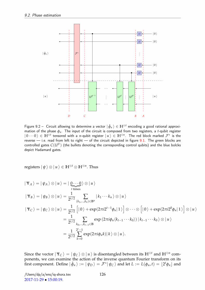
9.2. Phase estimation
F ∗
| 0 〉H
| 0 〉H
| 0 〉H
| 0 〉H•
•
•
| u 〉
| φu 〉 ...
U20U21
U2t−1
. . .
...
. . .
| u 〉......
ABCD
Figure 9.2 – Circuit allowing to determine a vector | φu 〉 ∈ H⊗t encoding a good rational approxi-mation of the phase φu. The input of the circuit is composed from two registers, a t-qubit register| 0 · · · 0 〉 ∈ H⊗t tensored with a n-qubit register | u 〉 ∈ H⊗n. The red block marked F ∗ is thereverse — i.e. read from left to right — of the circuit depicted in figure 9.1. The green blocks arecontrolled gates C(U2j
) (the bullets denoting the corresponding control qubits) and the blue bolcksdepict Hadamard gates.
registers |ψ 〉 ⊗ | u 〉 ∈H⊗t ⊗H⊗n. Thus
|ΨA 〉 = |ψA 〉 ⊗ | u 〉 = | 0 · · · 0︸ ︷︷ ︸t times
〉 ⊗ | u 〉
|ΨB 〉 = |ψB 〉 ⊗ | u 〉 =1
2t/2 ∑(k1,...,kn)∈Bn
| k1 · · · kn 〉 ⊗ | u 〉
|ΨC 〉 = |ψC 〉 ⊗ | u 〉 =1
2t/2
[| 0 〉+ exp(2πi2t−1φu| 1 〉
]⊗ · · · ⊗
[| 0 〉+ exp(2πi20φu| 1 〉
]⊗ | u 〉
=1
2t/2 ∑k0,...,kt−1∈B
exp (2πiφu〈kt−1 · · · k0〉) | kt−1 · · · k0 〉 ⊗ | u 〉
=1
2t/2
2t−1
∑k=0
exp(2πiφuk)| k 〉 ⊗ | u 〉.
Since the vector |ΨC 〉 = |ψC 〉 ⊗ | u 〉 is disentangled between its H⊗t and H⊗n com-ponents, we can examine the action of the inverse quantum Fourier transform on itsfirst component. Define | φu 〉 := |ψD 〉 = F ∗|ψC 〉 and let L := L(φu, t) = b2tφuc and
/Users/dp/a/ens/iq-shora.tex2017-11-29 • 15:00:19.
126
The Shor’s factoring algorithm
0 ≤ δ := δ(φu, t) = φu − L2t < 1. We have then
| φu 〉 =1
2t/2
2t−1
∑k=0
exp(2πiφuk)F ∗| k 〉
=12t
2t−1
∑k=0
exp(2πiφuk)2t−1
∑l=0
exp(−2πikl
2t )| l 〉
=12t
2t−1
∑k,l=0
exp(2πiφuk) exp(−2πikl + L
2t )| L + l mod 2t 〉
=2t−1−1
∑l=−2t−1
2t−1
∑k=0
[12t exp
(−2πi(δ− l
2t )
)k]
︸ ︷︷ ︸αl
| L + l mod 2t 〉.
Now, for l ∈ 0, . . . , 2t − 1, we can compute explicitely
αl =
10(l) if δ = 0,12t
exp(−πi(2tδ−l))exp
(−πi(δ− l
2t )) sin(π(2tδ−l))
sin(
π(δ− l2t )) if 0 < δ < 1.
If φu is exactly expressible as the dyadic rational L2t , i.e. δ = 0, then obviously | φu 〉 =
| L 〉 and the theorem holds with ε = 0 and ∆ = L. In the other cases, it turns outthat |αl|2 is sharply peaked around 0 (see figure 9.3 for an example). The end of theproof consists in finding the smallest ∆ so that Pφu
(∆c) < ε. First remark that for
−π2 < θ < π
2 we have | sin(θ)| ≥ 2|θ|π . Therefore, by writing
|αl| =12t
∣∣sin(π(2tδ− l)
)∣∣∣∣∣sin(
π(δ− l2t ))∣∣∣ ≤ 1
2t1∣∣∣sin
(π(δ− l
2t ))∣∣∣ ,
we conclude that |αl|2 ≤ 14|l|2 . Suppose now that ∆M = L − M mod 2t, . . . , L + M
mod 2t for some integer M ≤ 2t−1 and consider the effect E[∆M] = ∑m∈∆M|m 〉〈m |.
Then
Pφu(∆M) = ∑
m∈∆M
〈 φu |m 〉〈m | φu 〉
= ∑m∈∆M
2t−1−1
∑l,l′=−2t−1
αlαl′〈 L + l mod 2t |m 〉〈m | L + l′ mod 2t 〉
= ∑m∈∆M
|αm−L mod 2t |2 =M
∑m=−M
|αm|2.
We must now optimise M so that M2t = O( 1
2n ) and Pφu(∆c
M) < ε. We estimate
Pφu(∆c
M) ≤ 22t−1−1
∑m=M
|αl|2 ≤2t−1−1
∑m=M
12m2 ≤
12M≤ ε,
/Users/dp/a/ens/iq-shora.tex2017-11-29 • 15:00:19.
127

9.3. Order finding
and
max|m + L mod 2t
2t − φu|, m ∈ ∆M =M2t ≤
12n .
The choice p = d− log2 εe+ 1 and t = n + p establishes the conclusion of the theorem.
Figure 9.3 – Example values of |αl |2 for l ∈ −16, . . . , 15 for the case t = 10 and δ = 0.2. Onlythe values near 0 are depicted since the values in the range −512, . . . , 511 \ L− 16, . . . , 15 areso small that are represented by points lying beneath the threshold of graphical discrimination from0.
We can summarise the results obtained so far, in the algorithm 9.2.3.
Algorithm 9.2.3. Phase estimation
Require: Black boxes C(U2j),
eigenvector | u 〉 of U,precision threshold ε,t = n + dlog(2 + 1
2εe qubits initialised at | 0 〉.Ensure: Estimation of φu precise up to t bits.
Initialise | 0 〉⊗t ⊗ | u 〉.Apply operators as in regions A− C of figure 9.3 .Apply F ∗ on the t first qubits register to get | φu 〉.Mesure the t-qubit register to obtain estimation of φu
9.3 Order finding
9.3.1 The order finding problem
Definition 9.3.1. Let x, N be fixed integers strictly larger than 1 with pgcd(x, N) = 1.We define the order of x in N by
ord(x, N) = infr > 0 : xr = 1 mod N.
/Users/dp/a/ens/iq-shora.tex2017-11-29 • 15:00:19.
128

The Shor’s factoring algorithm
It is conjectured that the problem of order finding is an algorithmically hard prob-lem. As a matter of fact, if L = dlog Ne, we don’t know any classical algorithm solvingthis problem in polynomial (in L) time. For an L-bit string y = y1 . . . yL ∈ BL, denoteby y = 〈y〉 ∈ 0, . . . , 2L − 1. These integers serve as an indexing set for the canonicalbasis and | y 〉 = | y1 . . . yL 〉 ∈H⊗L, with H = C2.
Definition 9.3.2. For x and N as in definition 9.3.1, L = dlog Ne, and | y 〉 ∈ H⊗L,define the unitary operator
U| y 〉 =| xy mod N 〉 if 0 ≤ y ≤ N − 1,| y 〉 if N ≤ y ≤ 2L − 1.
Lemma 9.3.3. Let r := ord(x, N) ≤ N. For s = 0, . . . , r− 1, and
| us 〉 =1√r
r−1
∑k=0
exp(−2πiksr)| xk mod N 〉,
we have1. that the vector | us 〉 is an eigenvector of U:
U| us 〉 = exp(2πisr)| us 〉;
2. that the vector | 1 〉 is a linear combination of eigenvectors:
1√r
r−1
∑s=0| us 〉 = | 1 〉.
Proof. 1. We compute plainly
U| us 〉 =1√r
r−1
∑k=0
exp(−2πiks/r)| xk+1 mod N 〉
=1√r
r
∑k=1
exp(−2πi(k− 1)s/r)| xk mod N 〉
=1r
exp(2πis/r)
(r−1
∑k=1
exp(−2πiks/r)| xk mod N 〉+ | xr mod N 〉)
= exp(2πis/r)| us 〉.
2. Since ∑r−1s=0 exp(−2πisk/r) = rδk,0, we compute
1√r
r−1
∑s=0| us 〉 =
1r
exp(−2πisk/r)| xk mod N 〉 = | 1 〉.
Remark 9.3.4. The lemma 9.3.3 establishes that for every s, the construction of thevector | us 〉 supposes previous knowledge of r. Item 2 of this lemma is of the utmostimportance for the feasibility of the algorithm because it suggests that instead of ini-tialising the algorithm with | us 〉 it is enough to initialise with | 1 〉 and the result willbe a linear combination of actions of U.
/Users/dp/a/ens/iq-shora.tex2017-11-29 • 15:00:19.
129

9.3. Order finding
9.3.2 Classical continued fraction expansion
If we are able to determine the ratio s/r for different values of s, we shall be ableto estimate r and the problem of order finding will be solved. This estimation problemis solved by the classical algorithm of continued fraction expansion. Let recall brieflywhat is the continued fraction expansion.
We associate with every α ∈ R+ a (finite or infinite) sequence of (a0; a1, a2, · · · ) suchthat α can be decomposed into the continued fraction expansion (CFE)
α = a0 +1
a1 +1
a2 +1
a3 +1...
.
The terms a1, a2, . . . appearing in this expansion are in N>, the term a0 — correspond-ing to bαc — can take also the value 0. We write α = [a0; a1, a2, a3, . . .] to denote theprevious expansion.
— If α ∈ Q+, there exists a M > 0 such that the sequence defining the CFE of α isfinite, i.e. α = [a0; a1 . . . , aM].
— If α ∈ (R+ \Q), its CFE is given by an infinite sequence α = [a0; a1, a2, a3, . . .],with ai > 0 for all i ≥ 1.
If α is represented by an infinite expansion α = [a0; a1, a2, . . .], then its truncated (atorder m) expansion [a0; a1 . . . , am] is a rational approximation of α. As a matter of fact,
[a0; a1 . . . , am] =pm(α)
qm(α),
where pm := pm(α) and qm := qm(α) are integers defined by the recursive relations:
pm = am pm−1 + pm−2 and qm = amqm−1 + qm−2, m ≥ 1,
and p0 = a0, q0 = 1, p−1 = 1, and q−1 = 0. The sequence of ratios pm(α)qm(α)
are calledprincipal convergent of α.
Lemma 9.3.5. (See [46, chapter 1]). Denote by αm = [a0; a1 . . . , am] = pm/qm the sequenceof principal convergents.
1. α0 ≤ α2m ≤ α2m+2 ≤ . . . α ≤ . . . ≤ α2m+1 ≤ α2m−1 ≤ . . . α1 and limm→∞ :=limm→∞
pm(α)qm(α)
= α.
2. Let pq be an irreducible fraction with q > 0. If
|α− pq| ≤ 1
2q2
then there exists an M such that pq = αM, i.e. the sequence of principal convergents
verifies |α− pmqm| ≤ 1
2q2m
for all m ∈N>.
/Users/dp/a/ens/iq-shora.tex2017-11-29 • 15:00:19.
130

The Shor’s factoring algorithm
The classical algorithm 9.3.6 summarises the construction of the (truncated) CFE.
Algorithm 9.3.6. Continued fraction expansion (CFE)Require: real α > 0, integer M > 0.Ensure: a0, . . . , aM with ai > 0 pour 1 ≤ i ≤ M.
Initialise m← 0.repeat
am ← bαc.β← α (It is recalled that α := α− bαc).m← m + 1.if β 6= 0 then
α← 1β
elseα← 0
end ifuntil m > M.
9.3.3 Order finding algorithm
The order finding algorithm — summarised in 9.3.8 below — is in fine a phase es-timation algorithm for a particular unitary operator U = Ux,N, for x and N fixed pos-itive coprime integers (i.e. gcd(x, N) = 1). Denote by L = log2 Ne the number of bitsrequired to represent N and set t = 2L + 1.
Proposition 9.3.7. Let x, N, and L as above.1. Consider the circuit depicted in figure 9.3 instanciated with U := Ux,N and initialised
with | 0 〉 ⊗ | us 〉 ∈ H⊗t ⊗H⊗n. Measuring in the state of the first register |ψD 〉 =| s/r 〉 provides with an approximation θ of the phase s/r.
2. Applying the CFE algorithm on this approximation determines the order r with largeprobability.
3. If the second register of the initialisation vector is set at | 1 〉 ∈ H⊗n, the vector |ΨD 〉reads 1√
r ∑r−1s=0 | s/r 〉 ⊗ | us 〉.
Proof. 1. When the circuit is initialised with | 0 〉⊗ | us 〉 ∈H⊗t⊗H⊗n, the registersat position C read
|ΨC 〉 =1
2t/2
2t−1
∑k=0
exp(
2πisr
k)| k 〉 ⊗ | us 〉.
We conclude by theorem 9.2.2 that
|ΨD 〉 = (F ∗ ⊗ I)|ΨC 〉 = | s/r 〉 ⊗ | us 〉
and measuring in that vector yields s/r with large probability.
/Users/dp/a/ens/iq-shora.tex2017-11-29 • 15:00:19.
131

9.3. Order finding
2. Since θ is an 2L+ 1-bit approximation of s/r, it follows that |θ− r/s| ≤ 2−2L−1 ≤1/2r2 because r ≤ N 2L. Hence, by lemma ??, the approximation φ is the con-tinued fraction expansion of s/r. Therefore, the continued fraction expansionyields numbers r′ and s′ without common factors verifying s′/r′ = s/r. Thenumber r′ is a good candidate for ord(x, N). It is effectively the order if xr′ = 1mod N. And this happens with high probability.
3. The result follows by linearity since | 1 〉 = 1√r ∑r−1
s=0 | us 〉.
The proposition 9.3.7 guarantees that the algorithm 9.3.8 solves the order findingproblem.
Algorithm 9.3.8. Order finding algorithm (OFA)Require: Integer N with L bits,
x comprime with N,precision threshold ε,t = L + d− log2 εe qubits initialised at | 0 〉,L qubits initialised at | 1 〉,implementation of unitary UN,x : H⊗t ⊗H⊗L →H⊗t ⊗H⊗L,CFE algorithm.
Ensure: ord(x, N) with probability 1− ε within O(L3) steps.
Act as in figure 9.3 to get state |ψD 〉.Measure in state |ψD 〉 to get L-bit approximation θ of the phase.a := [a0; a1, . . . , an]← CFE(θ).sr ←
pn(a)qn(a)
.if xr mod N = 1 then
return relse
The algorithm fails.end if
Let us examine when the algorithm can fail:— A first possibility is that the algorithm produces an false estimate of the phase
s/r. This can occur with probability less than ε at the expense of a size d− log2 εeof the circuit.
— A second possibility is that s and r have a common factor. In that case, the ratioreturned by the OFA is an irreducible fraction s′/r′ equal to s/r. In that case, thevalue r′ determined by the algorithm is not the true order but only a factor of it.
Suppose that we run the algorithm 9.3.8 twice and let s′1, r′1 and s′2, r′2 be the valuesdetermined by each run. Provided that s′1 and s′2 have no common factor, the truevalue r can be determined by taking r = lcm(r′1, r′2). Proposition 9.3.9 minorises theprobability to obtain the correct answer r.
Proposition 9.3.9.
P(r is the correct order ) ≥ 14
.
/Users/dp/a/ens/iq-shora.tex2017-11-29 • 15:00:19.
132

The Shor’s factoring algorithm
Proof. For two positive integers x and y denote by x|y the fact that x divides y. Theprobability that s′ and s′ have no common factor is given by
P(s′ and s′′ have a common factor ) = 1− ∑p∈ primes
P(p|s′1)P(p|s′2).
Now, if p divides s′1 then it must also divide the value s. To majorise P(p|s′1) it isenough to majorise P(p|s1) where s1 is chosen uniformly at random in 0, . . . , r −1. In that case P(p|s1) = P(s ∈ p, 2p, . . . , kp) with kp < r; therefore P(s ∈p, 2p, . . . , kp) ≤ 1
p . Hence
1− ∑p∈ primes
P(p|s′1)P(p|s′2) ≥ 1− ∑p∈ primes
1p2 ≥ 1− ∑
p≥2
1p2 ≥
14
.
Exercise 9.3.10. Show that the lower bound 1/4 in the above proposition can be arbi-trarily improved at the expense of several independent repetitions of the procedure.
9.4 Shor’s factoring algorithm
Shor’s algorithm exploits the algorithmic efficacy of the quantum order finding al-gorithm to solve the factoring problem within polynomial time.
The algorithm relies on lemmata 9.4.1 and 9.4.2.
Lemma 9.4.1. Let N be a composite number representable within L bits. Suppose that x isa non-trivial solution to x2 = 1 mod N for x ∈ 1, . . . , N (i.e. neither x = 1 mod Nnor x = N − 1 mod N = −1 mod N hold). Then at least one of gcd(x − 1, N) andgcd(x + 1, N) is a non-trivial factor of N (computable within O(L3) steps).
Proof. Since x2 = 1 mod N it follows that N divides x2 − 1 = (x − 1)(x + 1); henceN must have a common factor with one of the terms x − 1 or x + 1. However, 1 <x < N − 1 by assumption. Therefore, N cannot be a common factor of either x− 1 orx + 1. Then at least one of gcd(x− 1, N) and gcd(x + 1, N) is a non-trivial factor of N.Euclid’s algorithm determines the gcd in O(L3) operations.
Lemma 9.4.2. Let N = pn11 . . . pnm
m be the prime factoring of an odd composite integer N andx a random integer, uniformely chosen in 1, . . . , N− 1 under the condition of being coprimewith N, and r = ord(x, N). Then
P(r is even and xr/2 6= −1 mod N) ≥ 1− 12m .
Proof. See [55, §A4.3] for instance.
/Users/dp/a/ens/iq-shora.tex2017-11-29 • 15:00:19.
133

9.5. Scalability requirements to implement Shor’s algorithm
Shor’s factoring algorithm is summarised in 9.4.3. Its efficiency is estimated bythe number of gates required for modular exponentiation and order finding. Thosetasks can be achieved by using a total of O(L3) gates and this resource requirementdetermines also the time complexity of the algorithm.
Algorithm 9.4.3. Shor’s factoring algorithmRequire: Composite integer N with L bits,
OFA.Ensure: A non-trivial factor of N with probability O(1) within O(L3) steps.
if N is even thenreturn 2. End.
end ifif N = ab for integers a ≥ 1 and b ≥ 2 then
return a. End.end ifRandomly choose x ∈ 1, . . . , N − 1if f = gcd(x, N) > 1 then
return f . End.end ifUse OFA to find r = ord(x, N)if r is even and xr/2 6= −1 mod N then
f1 = gcd(xr/2 − 1, N) and f2 = gcd(xr/2 + 1, N)end ifif f1 is a factor then
return f1. End.end ifif f2 is a factor then
return f2. End.else
the algorithm fails. End.end if
9.5 Scalability requirements to implement Shor’s algo-rithm
Section to be re-written
The naïve resource scaling O(L3) quoted in the previous section presupposes aflawless functioning of quantum gates. However, this is only an idealisation of thephysical process. Error correction codes are needed in all steps to control the analogquantum gates.
To factor an L-bit integer N with full fledged — i.e. including error corrections —
/Users/dp/a/ens/iq-shora.tex2017-11-29 • 15:00:19.
134

The Shor’s factoring algorithm
Shor’s algorithm, we need (see [13]):— 5L + 1 qubits,— 72L3 quantum gates.A simple numerical application:
L = 4: 21 qubits, 4608 gates,
L = 100: 501 qubits, 7.2× 10⁷ gates,
L = 4096: 20481 qubits, 4.95× 10¹² gates.
Shor’s algorithm: — 15 = 3× 5 (k = 4). Factored by using 7 qubits.— 21 = 3× 7 (k = 5). Factored by using 10 qubits [53].
Optimisation: — 143 = 11 × 13 (with 4 qubits) and 56153 = 233 × 241 (with 4qubits) [86].
— Foreseen — not yet implemented — factoring of 291311 = 523× 557 with 6qubits [29].
/Users/dp/a/ens/iq-shora.tex2017-11-29 • 15:00:19.
135

9.5. Scalability requirements to implement Shor’s algorithm
/Users/dp/a/ens/iq.tex2018-01-20 • 17:20:00.
136

Part III
Quantum mechanics in infinitedimensional spaces
137


10Algebras of operators
10.1 Introduction and motivation
Let V = Cn, with n ∈N. Elementary linear algebra establishes that the set of linearmappings L(V) = T : V→ V : T linear is a C-vector space of (complex) dimensionn2, isomorphic to Mn(C), the space of n× n matrices with complex coefficients. More-over, if S, T ∈ L(V), the maps S and T can be composed, their composition T S beingrepresented by the corresponding matrix product. Thus, on the vector space L(V), isdefined an internal multiplication
L(V)× L(V) 3 (T, S) 7→ T S ∈ L(V)
turning this vector space into an algebra.
When the underlying vector space V is of infinite dimension, caution must be paidon defining linear maps. In general, linear mappings T : V → V, called (linear)operators, are defined only on some proper subset of V denoted Dom(T) and calledthe domain 1 of T. When V is a normed space, there is a natural way to define a normon L(V). We denote by B(V) the vector space of bounded linear operators on V, i.e.linear maps T : V → V such that ‖T‖ < ∞ (equivalently, verifying Dom(T) = V.)When H is a Hilbert space, bounded linear operators on H, whose set is denoted byB(H), with operator norm ‖T‖ = sup‖Tx‖, x ∈ H, ‖x‖ ≤ 1, share the propertiesof linear operators defined on more algebraic setting. Sometimes it is more efficient towork with explicit representations of operators in B(H) (that play the rôle of matricesin the infinite dimensional setting) and some others with abstract algebraic setting.
Since all operators encountered in quantum mechanics are linear, we drop hence-forth the adjective linear.
1. The set Dom(T) is generally a vector subspace of V which is not necessarily topologically closed.
139

10.2. Algebra of operators
10.2 Algebra of operators
Definition 10.2.1. An algebra is a set A endowed with three operations:
1. a scalar multiplication C×A 3 (λ, a) 7→ λa ∈ A,
2. a vector addition A×A 3 (a, b) 7→ a + b ∈ A, and
3. a vector multiplication A×A 3 (a, b) 7→ ab ∈ A,
such that A is a vector space with respect to scalar multiplication and vector additionand a ring (not necessarily commutative) with respect to vector addition and vectormultiplication. Moreover, λ(ab) = (λa)b = a(λb) for all λ ∈ C and all a, b ∈ A. Thealgebra is called commutative if ab = ba, for all a, b ∈ A; it is called unital if there exists(a necessarily unique) element e ∈ A (often also written 1 or 1A) such that ae = ea = afor all a ∈ A;
A linear map from an algebra A1 to an algebra A2 is a homomorphism if it is aring homomorphism for the underlying rings, it is an isomorphism if it is a bijectivehomomorphism.
Definition 10.2.2. An involution on an algebra A is a map A 3 a 7→ a∗ ∈ A thatverifies
1. (λa + µb)∗ = λa∗ + µb∗,
2. (ab)∗ = b∗a∗, and
3. (a∗)∗ = a.
Involution is also called adjoint operation and a∗ the adjoint of a. An involutive alge-bra is termed a ∗-algebra.
An element a ∈ A is said normal if aa∗ = a∗a, an isometry if a∗a = 1, unitary if botha and a∗ are isometries, self-adjoint or Hermitean if a = a∗. On denoting h : A1 → A2 ahomomorphism between two ∗-algebras, we call it a ∗-homomorphism if it preservesadjoints, i.e. h(a∗) = h(a)∗.
A normed (respectively Banach) algebra A is an algebra equipped with a norm map‖ · ‖ : A → R+ that is a normed (respectively Banach) vector space for the norm andverifies ‖ab‖ ≤ ‖a‖‖b‖ for all a, b ∈ A. A is normed (respectively Banach) ∗-algebra ifit has an involution verifying ‖a∗‖ = ‖a‖ for all a ∈ A.
Theorem 10.2.3. Let T : H1 →H2 be a linear map between two Hilbert spaces H1 and H2.Then the following are equivalent:
1. ‖T‖ = sup‖T f ‖H2 , f ∈H1, ‖ f ‖H1 ≤ 1 < ∞,
2. T is continuous,
3. T is continuous at one point of H1.
Proof: Analogous to the proof of the theorem ?? for linear functional. (Please completethe proof!)
/Users/dp/a/ens/iq-algop.tex2015-09-16 • 14:44:15.
140

Algebras of operators
Notation 10.2.4. We denote by B(H1, H2) the algebra of bounded operators withrespect to the aforementioned norm:
B(H1, H2) = T ∈ L(H1, H2) : ‖T‖ < ∞.
When H1 = H2 = H, we write simply B(H).
Proposition 10.2.5. Let H1 and H2 be two Hilbert spaces and T ∈ B(H1, H2). Then, thereexists a unique bounded operator T∗ : H2 →H1 such that
〈 T∗g | f 〉 = 〈 g | T f 〉 for all f ∈H1, g ∈H2.
Proof: For each g ∈ H2, the map H1 3 f 7→ 〈 g | T f 〉H2∈ C is a continuous (why?)
linear form. By Riesz-Fréchet theorem ??, there exists a unique h ∈ H1 such that〈 h | f 〉H1
= 〈 g | T f 〉H2, for all f ∈ H1. Let T∗ : H2 → H1 be defined by the as-
signment T∗g = h; it is obviously linear and easily checked to be bounded (exercise!)
Proposition 10.2.6. For all T ∈ B(H1, H2),
1. ‖T∗‖ = ‖T‖,2. ‖T∗T‖ = ‖T‖2.
Proof:
1. By Cauchy-Schwarz inequality, for all f ∈H2, g ∈H1,
|〈 f | Tg 〉H2| ≤ ‖ f ‖H2‖Tg‖H2
≤ ‖T‖B(H1,H2)‖g‖H1‖ f ‖H2
so that‖T‖ ≥ sup|〈 f | Tg 〉| : ‖g‖ ≤ 1, ‖ f ‖ ≤ 1.
Conversely, we may assume that ‖T‖ 6= 0, and therefore choose some ε ∈]0, ‖T‖/2[. Choose now g ∈ H1 with ‖g‖ ≤ 1, such that ‖Tg‖ ≥ ‖T‖ − ε
and f = Tg‖Tg‖ ∈H2, ‖ f ‖ = 1. For this particular choice of f and g:
|〈 f | Tg 〉H2| ≥ ‖Tg‖ ≥ ‖T‖ − ε.
Hence,sup|〈 f | Tg 〉| : ‖g‖ ≤ 1, ‖ f ‖ ≤ 1 ≥ ‖T‖ − ε.
Since ε is arbitrary, we get ‖T‖ = sup|〈 f | Tg 〉H2| : g ∈ H1, f ∈ H2, ‖g‖ ≤
1, ‖ f ‖ ≤ 1. As 〈 f | Tg 〉 = 〈 T∗ f | g 〉 for all f and g, we get ‖T∗‖ = ‖T‖2. B(H1, H2) being a normed algebra, ‖T∗T‖ ≤ ‖T∗‖‖T‖ = ‖T‖2. Conversely,
‖T‖2 ≤ sup|T f ‖ : f ∈H1, ‖ f ‖ ≤ 1= sup|〈 T f | T f 〉| : f ∈H1, ‖ f ‖ ≤ 1= sup|〈 f | T∗T f 〉| : f ∈H1, ‖ f ‖ ≤ 1≤ ‖T∗T‖.
/Users/dp/a/ens/iq-algop.tex2015-09-16 • 14:44:15.
141

10.3. Convergence of sequences of operators
Definition 10.2.7. A C∗-algebra A is an involutive Banach algebra verifying addition-ally
‖a∗a‖ = ‖a‖2, for all a ∈ A.
Example 10.2.8. Let X be a compact Hausdorff 2 space and
A = f : X→ C | f continuous ≡ C(X).
Define
1. C×A 3 (λ, f ) 7→ λ f ∈ A by (λ f )(x) = λ f (x), ∀x ∈ X,
2. A×A 3 ( f , g) 7→ f + g ∈ A by ( f + g)(x) = f (x) + g(x), ∀x ∈ X,
3. A×A 3 ( f , g) 7→ f g ∈ A by ( f g)(x) = f (x)g(x), ∀x ∈ X,
4. A 3 f 7→ f ∗ ∈ A by f ∗(x) = f (x), ∀x ∈ X,
Then A is a unital (specify the unit!) C∗-algebra for the norm ‖ f ‖ = supx∈X | f (x)|.(Prove it!) The algebra A is moreover commutative.
Example 10.2.9. Let H1 and H2 be two Hilbert spaces. Then B(H1, H2) is a unitalC∗-algebra. In general, this algebra is not commutative.
This example has also a converse, given in theorem 10.5.2, below.
Example 10.2.10. Let X be a compact Hausdorff space. Then
A = C(X) := f : X→ C, continuous
equipped with the uniform norm and pointwise multiplication is a unital Banach com-mutative algebra; further equipped with an involution defined by complex conjuga-tion, becomes a B∗-algebra.
Example 10.2.11. A = `1(Z), with à compléter.
Example 10.2.12. A = L1(R), with à compléter.
The previous example must not induce the reader to erroneously conclude thatnon-unital algebras have natural approximate identities since à compléter.
10.3 Convergence of sequences of operators
10.4 Classes of operators in B(H)
We shall see that any C∗-algebra can be faithfully represented on some Hilbert spaceH; the different classes of abstract elements of the algebra, introduced in the previ-ous section, have a counterpart in the context of this representation. But additionally,B(H) is a very special C∗-algebra because is closed for the weak operator topology
2. Recall that a topological space is called Hausdorff when every two distinct of its points possessdisjoint neighbourhoods.
/Users/dp/a/ens/iq-algop.tex2015-09-16 • 14:44:15.
142

Algebras of operators
(defined in §10.3). This fact endows B(H) with a very rich family of projections allow-ing to generate 3 back the unital C∗-algebra B(H).
10.4.1 Self-adjoint and positive operators
Definition 10.4.1. An operator T ∈ B(H) is called self-adjoint or Hermitean 4 ifT = T∗. The set of Hermitean operators on H is denoted by Bh(H).
Exercise 10.4.2. The operator T ∈ B(H) is self-adjoint if and only if 〈 f | T f 〉 ∈ R forall f ∈H. (Hint: use the polarisation equality ??.)
Exercise 10.4.3. If T ∈ B(H) is self-adjoint then ‖T‖ = sup〈 f | T f 〉, f ∈ H, ‖ f ‖ ≤1.
Definition 10.4.4. An operator T ∈ B(H) is called positive if 〈 f | T f 〉 ≥ 0 for allf ∈ H. Such an operator is necessarily self-adjoint. We denote by B+(H) the set ofpositive operators.
Exercise 10.4.5. Show that T ∈ B+(H) if and only if there exists S ∈ B(H) such thatT = S∗S.
10.4.2 Projections
Definition 10.4.6. Let P, P1, P2 ∈ B(H).
1. P is a projection if P2 = P.2. P is an orthoprojection if is a projection satisfying further P∗ = P.3. Two orthoprojections P1, P2 ∈ B(H) are orthogonal, denoted P1 ⊥ P2 of their
images are orthogonal subspaces of H (equivalently P1P2 = 0).
Projections are necessarily positive (why?). The set of orhoprojections is denotedby P(H). All projections considered henceforth will be orthoprojections.
Exercise 10.4.7. (A very important one!) Let (Pn) be a sequence of orthoprojections.We have already shown that there is a bijection between P(H) and the set of closedsubspaces of H and orthoprojections, given by P(H) 3 P 7→ P(H) ⊂ H, with P(H)closed.
1. Show that that P(H) is partially ordered, i.e. P1 ≤ P2 if P1(H) subspace ofP2(H) (equivalently P1P2 = P1.)
2. For general orthoprojections P1 and P2, is P1P2 an orthoprojection?3. Show that P1 and P2 have a least upper bound.4. Is Q = P1 + . . . + Pn an orthoprojection?5. Is Q = P2 − P1 an orthoprojection?
3. In some general unital C∗-algebras there are only two trivial projections 0 and 1. Therefore thesituation arising in B(H) is far from being a general property of C∗-algebras.
4. Strictly speaking, the term Hermitean is more general; it applies also to unbounded operators andit means self-adjoint on a dense domain. The two terms coincide for bounded operators.
/Users/dp/a/ens/iq-algop.tex2015-09-16 • 14:44:15.
143

10.4. Classes of operators in B(H)
6. Show that a monotone sequence of orthoprojections converges strongly towardsan orthoprojection.
10.4.3 Unitary operators
Definition 10.4.8. An operator U ∈ B(H) is unitary if U∗U = UU∗ = 1. The set ofunitary operators is denoted by U(H) = U ∈ B(H) : U∗U = UU∗ = 1 (it is in facta group; for H = Cn it is the Lie group denoted by U(n).)
10.4.4 Isometries and partial isometries
Definition 10.4.9. An operator T ∈ B(H1, H2) is an isometry if T∗T = 1 (or equiva-lently ‖T f ‖ = ‖ f ‖, for all f ∈H1.)
Exercise 10.4.10. Let H = `2(N) and for x = (x1, x2, x3, . . .) ∈ H, define the left andright shifts by
Lx = (x2, x3, . . .) ∈H,
andRx = (0, x1, x2, x3, . . .) ∈H.
1. Show that R∗ = L.
2. Show that R is an isometry.
3. Determine RanR.
This exercise demonstrates that, in infinite dimensional spaces, isometries are notnecessarily surjective.
Theorem 10.4.11. For T ∈ B(H1, H2), the five following conditions are equivalent:
1. (T∗T)2 = T∗T,
2. (TT∗)2 = TT∗,
3. TT∗T = T,
4. T∗TT∗ = T∗,
5. there exist closed subspaces E1 ⊆ H1 and E2 ⊆ H2 such that T = I S P whereP : H1 → E1 is a projection, S : E1 → E2 an isometry, and I : E2 →H2 the inclusionmap.
If one (hence all) condition holds then T∗T is the projection H1 → E1 and TT∗ is the projectionH2 → E2. In this situation T is called a partial isometry with initial space E1, initialprojection T∗T, final space E2, and final projection TT∗.
Proof. Exercise! (See [4] or [68].)
Exercise 10.4.12. Let (Ω,F , P) be a probability space and T : Ω → Ω a measurepreserving transformation i.e. P(T−1B) = P(B) for all B ∈ F . On the Hilbert spaceH = L2(Ω,F , P) define U : H→H by U f (ω) = f (T−1ω).
/Users/dp/a/ens/iq-algop.tex2015-09-16 • 14:44:15.
144

Algebras of operators
1. Show that U is a partial isometry.
2. Under which condition is U surjective (hence unitary)?
10.4.5 Normal operators
Definition 10.4.13. An operator T ∈ B(H) is normal if T∗T = TT∗ (or equivalently if‖T∗ f ‖ = ‖T f ‖ for all f ∈H.)
Exercise 10.4.14. A vector f ∈ H \ 0 is called an eigenvector corresponding to aneigenvalue λ of an operator T ∈ B(H) if T f = λ f for some λ ∈ C. Show that if T isnormal and f1, f2 are eigenvectors corresponding to different eigenvalues then f1 ⊥ f2.(The proof goes as for the finite dimensional case.)
Exercise 10.4.15. Let M be the multiplication operator on L2[0, 1] defined by M f (t) =t f (t), t ∈ [0, 1]. Show that
1. M is self-adjoint (hence normal),
2. M has no eigenvectors.
Exercise 10.4.16. Choose some z ∈ C with |z| < 1 and consider ζ ∈ `2(N) given byζ = (1, z, z2, z3, . . .). Let L and R be the left and right shifts defined in exercise 10.4.10.
1. Show that R is not normal,
2. compute R∗ζ,
3. conclude that R∗ has uncountably many eigenvalues.
10.5 States on algebras, GNS construction, representations
Paragraphe incomplet.
Definition 10.5.1. Let A be an involutive Banach algebra. A representation on aHilbert space H of A is a ∗-homomorphism of A into B(H), i.e. a linear map π :A→ B(H) such that
1. π(ab) = π(a)π(b), ∀a, b ∈ A,
2. π(a∗) = π(a)∗, ∀a ∈ A,
The space H is called the representation space. We write (π, H), or Hπ if necessary.Two representations (π1, H1) and (π2, H2) are said to be unitarily equivalent if thereexists an isometry U : H1 → H2 such that for all a ∈ A, it holds Uπ1(a)U∗ = π2(a). Ifmoreover for every non zero element of A, π(a) 6= 0, then the representation is calledfaithful.
Theorem 10.5.2 (Gel’fand-Naïmark). If A is an arbitrary C∗-algebra, there exists a Hilbertspace H and a linear mapping π : A→ B(H) that is a faithful representation of A.
Proof: It can be found in [42, theorem 4.5.6, page 281].
/Users/dp/a/ens/iq-algop.tex2015-09-16 • 14:44:15.
145

10.5. States on algebras, GNS construction, representations
/Users/dp/a/ens/iq-sptba.tex2017-10-16 • 11:23:53.
146

11Spectral theory in Banach algebras
11.1 Motivation
In linear algebra one often encounters systems of linear equations of the type
T f = g (11.1)
with f , g ∈ Cn and T = (ti,j)i,j=1,...,n a n× n matrix with complex coefficients. Elemen-tary linear algebra establishes that this system of equations has solutions provided thatthe map f 7→ T f is surjective and the solution is unique provided that this map is in-jective. Thus the system has a unique solution for each g ∈ Cn provided that the mapis bijective, or equivalently the matrix T is invertible. This happens precisely whendet T 6= 0. However, this criterion of invertibility is of limited practical use even forthe elementary (finite-dimensional) case because det is too complicated an object to beefficiently computed for large n. For infinite dimensional cases, this criterion becomestotally useless since there is no infinite dimensional analogue of det that discriminatesbetween invertible and non-invertible operators T (see exercise 11.1.1 below!)
Another general issue connected with the system (11.1) is that of eigenvalues. Forevery λ ∈ C, denote by Vλ = f ∈ Cn : T f = λ f . For most choices of λ, the subspaceVλ is the trivial subspace 0; this subspace is not trivial only when T − λ1 is notinjective (i.e. ker(T − λ1) 6= 0.) On defining the spectrum of T by
spec(T) = λ ∈ C : T − λ1 is not invertible ,one easily shows that spec(T) 6= ∅ and card spec(T) ≤ n (why?) Not always the family(Vλ)λ∈spec(T) spans the whole space Cn. When it does, on decomposing g = g(1) +. . . + g(k) where g(j) ∈ Vλj and spec(T) = λ1, . . . , λk, the solution of (11.1) is given by
f =g(1)
λ1+ . . . +
g(k)
λk.
147

11.2. The spectrum of an operator acting on a Banach space
(Notice that λi 6= 0, for all i = 1, . . . , k; why?) When the family (Vλ)λ∈spec(T) does notspan Cn, the problem is more involved but the rôle of the spectrum remains funda-mental.
A final issue involving the spectrum of T is the functional calculus associated withT. If p ∈ R[t], this polynomial can be naturally extended on B(H). In fact, if p(t) =antn + . . . a0 is the expression of the polynomial p; the expression p(T) = anTn + . . . a01
is well defined for all T ∈ B(H). Moreover, if T ∈ Bh(H) then p(T) ∈ Bh(H).Suppose now that T ∈ Bh(H), m = inf‖ f ‖=1 〈 f | T f 〉, M = sup‖ f ‖=1 〈 f | T f 〉, andp(t) ≥ 0 for all t ∈ [m, M]; then p(T) ∈ B+(H). Now every f ∈ C[m, M] can beuniformly approximated by polynomials, i.e. there is a sequence (pl)l∈N, with pl ∈R[t] such that for all ε > 0, there exists n0 ∈ N such that for l ≥ n0, maxt∈[m,M] | f (t)−pl(t)| < ε. It is natural then to define f (T) = liml pl(T). However, the computationsinvolved in the right hand side of this equation can be very complicated. Supposehenceforth that H = Cn and T is a Hermitean n × n matrix that is diagonalisable,
i.e. T = UDU∗ with D =
λ1. . .
λn
and U unitary. Then pl(T) = Upl(D)U∗ and
letting l → ∞ we get f (T) = U f (D)U∗. Thus, if T is diagonalisable, the computation off (T) is equivalent to the knowledge of f (t) for t ∈ spec(T). For the infinite dimensionalcase, the problem is more involved but again the spectrum remains fundamental.
The rest of this chapter, based on [4], is devoted to the appropriate generalisationof the spectrum for infinite dimensional operators.
Exercise 11.1.1. (Infinite-dimensional determinant) Let H = `2(N) and (tn)n∈N bea fixed numerical sequence. Suppose that there exist constants K1, K2 > 0 such that0 < K1 ≤ tn ≤ K2 < ∞ for all n ∈N. For every x ∈ `2(N) define (Tx)n = tnxn, n ∈N.
1. Show that T ∈ B(H).2. Exhibit a bounded operator S on H such that ST = TS = 1.3. Assume henceforth that (tn)n∈N is a monotone sequence. Let ∆n(T) = t1 · · · tn.
Show that ∆n(T) converges to a non-zero limit ∆(T) if and only if ∑n(1− tn) <∞.
4. Any plausible generalisation, δ, of det in the infinite dimensional setting shouldverify δ(1) = 1, δ(AB) = δ(A)δ(B), and if T is diagonal δ(T) = ∆(T). Choos-ing tn = n
n+1 , for n ∈ N, conclude that although T is diagonal and invertible,nevetheless has δ(T) = 0.
11.2 The spectrum of an operator acting on a Banach space
Let V be a C-Banach space. Denote by B(V) the set of bounded operators T : V→V. This space is itself a unital Banach algebra for the induced operator norm.
Exercise 11.2.1. If X and Y are metric spaces and dX and dY denote their respectivemetrics
/Users/dp/a/ens/iq-sptba.tex2017-10-16 • 11:23:53.
148

Spectral theory in Banach algebras
1. verify that
dp((x1, y1), (x2, y2)) = (dX(x1, x2)p + dY(y1, y2)
p)1/p,
with p ∈ [1, ∞[ and
d∞((x1, y1), (x2, y2)) = max(dX(x1, x2), dY(y1, y2))
are metrics on X×Y; (the corresponding metric space (X×Y, dp), p ∈ [1, ∞] isdenoted 1 X⊕Y)
2. show that the sequence (xn, yn)n in X×Y converges to a point (ξ , ψ) ∈ X×Y
with respect to any of the metrics dp if and only if dX(xn, ξ)→ 0 and dY(yn, ψ)→0.
Exercise 11.2.2. Let X and Y be metric spaces and f : X → Y be a continuous map.We denote by
Γ( f ) = (x, f (x)) : x ∈ X
the graph of f . Show that Γ( f ) is closed (i.e. if (xn)n is a sequence in X and if thereexists (x, y) ∈ X×Y such that xn → x and f (xn)→ y, then necessarily y = f (x).)
Exercise 11.2.3. (The closed graph theorem) Suppose X and Y are Banach spaces andT : X→ Y a linear map having closed graph. Show that T is continuous.
Theorem 11.2.4. For every T ∈ B(V), the following are equivalent:
1. for every y ∈ V there is a unique x ∈ V such that Tx = y,
2. there is an operator S ∈ B(V) such that ST = TS = 1.
Proof: Only the part 1⇒ 2 is not trivial to show. Condition 1 implies that T is invertible;call S its inverse. The only thing to show is the boundedness of S. As a subset of V⊕V,the graph of S is related to the graph of T. In fact
Γ(S) = (y, Sy) : y ∈ V = (Tx, x), x ∈ V.
Now T is bounded, hence continuous, so that that the set (Tx, x), x ∈ V is closed(see exercise 11.2.2.) Thus the graph of S is closed, and by the closed graph theorem(see exercise 11.2.3), S is continuous hence bounded.
Definition 11.2.5. Let T ∈ B(V) where V is a Banach space.
1. T is called invertible if there exists an operator S ∈ B(V) such that ST = TS =1.
2. The spectrum of T, denoted by spec(T), is defined by
spec(T) = λ ∈ C : T − λ1 is not invertible.
3. The resolvent set of T, denoted by Res(T), is defined by
Res(T) = C \ spec(T).1. more precisely X⊕`p Y.
/Users/dp/a/ens/iq-sptba.tex2017-10-16 • 11:23:53.
149

11.3. The spectrum of an element of a Banach algebra
Notice that in finite dimension, invertibility of an operator R reduces essentially toinjectivity of R since surjectivity of R can be trivially verified if we reduce the space Vinto Ran(R). In infinite dimension, several things can go wrong: of course injectivitymay fail as in finite dimension; but a new phenomenon can appear when Ran(R) is notclosed: in this latter case, Ran(R) can further be dense in V or fail to be dense in V. Allthese situations may occur and correspond to different types of sub-spectra.
Definition 11.2.6. Let T ∈ B(V) where V is a Banach space.
1. The point spectrum of T is defined by
specp(T) = λ ∈ C : T − λ1 is not injective.
Every λ ∈ specp(T) is called an eigenvalue of T.
2. The continuous spectrum, specc(T), of T is defined as the set of complex valuesλ such that T− λ1 is injective but not surjective and Ran(T− λ1) is dense in V.
3. The residual spectrum, specr(T), of T is defined as the complex values λ suchthat T − λ1 is injective but not surjective and Ran(T − λ1) is not dense in V.
Example 11.2.7. Let V be a finite dimensional Banach space and T : V → V a lin-ear transformation (hence bounded.) Since dim ker(T − λ1) + dimRan(T − λ1) =dim V, it follows that T − λ1 is injective if and only if Ran(T − λ1) = V. There-fore specr(T) = ∅. Further, if T − λ1 is injective, then it has an inverse on V. Sinceany linear transformation of a finite dimensional space is continuous, it follows that(T − λ1)−1 is continuous, hence specc(T) = ∅. Therefore, in finite dimension we al-ways have spec(T) = specp(T).
Exercise 11.2.8. Let V = `2(N) and consider the right shift, R, on V.
1. Show that R− λ1 is injective for all λ ∈ C. Conclude that specp(R) = ∅.2. Show that for |λ| > 1, Ran(R− λ1) = V. Conclude that all λ ∈ C with |λ| > 1
belong to Res(R).3. For |λ| < 1, show that Ran(R−λ1) is orthogonal to the vector Λ = (1, λ, λ2, . . .).
Show that for |λ| < 1, Ran(R− λ1) = y ∈ V : y ⊥ Λ. Conclude that all λ ∈ C
with |λ| < 1 belong to specr(R).4. The case |λ| = 1 is the most difficult. Try to show that Ran(R− λ1) is dense in
V so that the unit circle coincides with specc(R).
11.3 The spectrum of an element of a Banach algebra
In the previous section we studied spectra of bounded operators acting on Banachspaces. They form a Banach algebra with unit. Spectral theory can be established alsoabstractly on Banach algebras. Before stating spectral properties, it is instructive togive some more examples.
Example 11.3.1. Let Cc(R) be the set of continuous functions on R which vanish out-side a bounded interval; it is a normed vector space (with respect to the L1 norm for
/Users/dp/a/ens/iq-sptba.tex2017-10-16 • 11:23:53.
150

Spectral theory in Banach algebras
instance; its completion is the Banach space L1(R, λ), where λ stands for the Lebesguemeasure.) A product can be defined by the convolution
f ? g(x) =∫
Rf (y)g(x− y)λ(dy)
turning this space into a commutative Banach algebra. This algebra is not unital (thiscan be seen by solving the equation f ? f = f in L1), but it has an approximate unit (i.e.a sequence ( fn)n of integrable functions with ‖ fn‖ = 1 for all n and such that for allg ∈ L1(R), ‖g ? fn − g‖ → 0. (Give an explicit example of such an approximate unit!)
Example 11.3.2. The algebra Mn(C) is a unital non-commutative algebra. There aremany norms that turn it into a finite-dimensional Banach algebra, for instance:
1. ‖A‖ = ∑ni,j=1 |ai,j|
2. ‖A‖ = sup‖x‖≤1‖Ax‖‖x‖ .
Definition 11.3.3. Let A be a unital Banach algebra. (We can always assume that‖1‖ = 1, may be after re-norming the elements of A.) An element a ∈ A is calledinvertible if there is an element b ∈ A such that ab = ba = 1. The set of all invertibleelements of A is denoted by GL(A) and called the general linear group of invertibleelements of A.
Theorem 11.3.4. Let A be a unital Banach algebra. If a ∈ A and ‖a‖ < 1 then 1− a isinvertible and
(1− a)−1 =∞
∑n=0
an.
Moreover,
‖(1− a)−1‖ ≤ 11− ‖a‖
and‖1− (1− a)−1‖ ≤ ‖a‖
1− ‖a‖ .
Proof: Since ‖an‖ ≤ ‖a‖n for all n, we can define b ∈ A as the sum of the absolutelyconvergent series b = ∑∞
n=0 an. Moreover, b(1− a) = (1− a)b = limN→∞ ∑Nn=0 bn =
limN→∞(1− bN+1) = 1. Hence 1− a is invertible and (1− a)−1 = b. The first ma-jorisation holds because ‖b‖ ≤ ∑∞
n=0 ‖a‖n = 11−‖a‖ . The second one follows from
remarking that 1− b = −∑∞n=1 an = −ab, hence ‖1− b‖ ≤ ‖a‖‖b‖.
Exercise 11.3.5. 1. Prove that GL(A) is an open set in A and that the mapping a 7→a−1 is continuous on GL(A).
2. Justify the term “general linear group” of invertible elements, i.e. show thatGL(A) is a topological group in the relative norm topology.
Definition 11.3.6. Let A be a unital Banach algebra. For every a ∈ A, the spectrum ofa is the set
spec(a) = λ ∈ C : a− λ1 6∈ GL(A).
In the rest of this section, A will be a unital algebra and we shall write a− λ insteadof a− λ1.
/Users/dp/a/ens/iq-sptba.tex2017-10-16 • 11:23:53.
151
11.3. The spectrum of an element of a Banach algebra
Proposition 11.3.7. For every a ∈ A, the set spec(a) is a closed subset of the disk λ ∈ C :|λ| ≤ ‖a‖.
Proof: Consider the resolvent set
Res(a) = λ ∈ C : a− λ ∈ GL(A) = C \ spec(a).
Since the set GL(A) is open (see exercise 11.3.5) and the map C 3 λ 7→ a − λ ∈ Acontinuous, the set Res(a) is open hence the set spec(a) is closed. Moreover, if |λ| >‖a‖, on writing a− λ = (−λ)[1− a/λ] and remarking that ‖a/λ‖ < 1, we concludethat a− λ ∈ GL(A).
Theorem 11.3.8. For every a ∈ A, the set spec(a) is non-empty.
Proof: Fix some λ0 ∈ Res(a). Since Res(a) is open, there is a small neighbourhood V≥of λ0 contained in Res(a). The A-valued function λ 7→ (a− λ)−1 is well defined for allλ ∈ V≥′ . Moreover, for λ, λ0 ∈ Res(a),
(a− λ)−1 − (a− λ0)−1 = (a− λ)−1[(a− λ0)− (a− λ)](a− λ0)
−1
= (λ− λ0)(a− λ)−1(a− λ0)−1.
Thus
limλ→λ0
1λ− λ0
[(a− λ)− (a− λ0)] = (a− λ0)−2.
Assume now that spec(a) = ∅ and choose an arbitrary bounded linear functionalφ : A→ C. Then, the scalar function f : C→ C defined by λ 7→ f (λ) = φ((a−λ)−1) isdefined on the whole C. By linearity, the function f has everywhere a complex deriva-tive, satisfying f ′(λ) = φ((a− λ)−2). Thus f is an entire function. Notice moreoverthat f is bounded and for |λ| > ‖a‖, by theorem 11.3.4,
‖(a− λ)−1‖ =‖(1− a/λ)−1‖
|λ|
≤ 1|λ|(1− ‖a‖/|λ|)
=1
|λ| − ‖a‖ .
Thus limλ→∞ f (λ) = 0 and since this function is bounded and entire, by Liouville’stheorem (see [?] for instance), it is constant, hence f (λ) = 0 for all λ ∈ C and everylinear functional φ. The Hahn-Banach theorem implies then that (a− λ)−1 = 0 for allλ ∈ C. But this is absurd because (a− λ) is invertible and 1 6= 0 in A.
Definition 11.3.9. For every a ∈ A, the spectral radius of a is defined by r(a) =sup|λ| : λ ∈ spec(a).
Exercise 11.3.10. 1. Let p ∈ R[t] and a ∈ A. Show that p(spec(a)) ⊆ spec(p(a)).(Hint: if λ ∈ spec(a), the map λ′ 7→ p(λ′)− p(λ) is a polynomial vanishing atλ′ = λ. Conclude that p(a)− p(λ) cannot be invertible.)
2. For every a ∈ A show that r(a) = limn→∞ ‖an‖1/n.
/Users/dp/a/ens/iq-sptba.tex2017-10-16 • 11:23:53.
152

Spectral theory in Banach algebras
11.4 Relation between diagonalisability and the spectrum
Motivated again by elementary linear algebra, we recall that a self-adjoint n× n ma-
trix T can be diagonalised, i.e. it is possible to find a diagonal matrix D =
d1. . .
dn
and a unitary matrix U such that T = UDU∗; we have then spec(T) = d1, . . . , dn. Weshall generalise this result to infinite dimensional spaces.
An orthonormal basis for H is a sequence E = (e1, e2, . . .) of mutually orthogonalunit vectors of H such that 2 spanE = H. On fixing such a basis, we define a unitaryoperator U : `2(N)→H by
U f = ∑i∈N
fiei
for f = ( f1, f2, . . .). Specifying a particular orthonormal basis in H is equivalent tospecifying a particular unitary operator U. Suppose now that T ∈ B(H) is a normaloperator and admits the basis vectors of E as eigenvectors, i.e. Tek = tkrk, tk ∈ C, k ∈N.Then t = (tk)k ∈ `∞(N) and U∗TU = M where M is the multiplication operatordefined by (M f )k = (U∗TU f )k = (U−1TU f )k = (U−1T ∑i fiei)k = fktk. Thus anoperator T on H is diagonalisable in a given basis E if the unitary operator associatedwith E implements an equivalence between T and a multiplication operator M actingon `2(N). This notion is still inadequate since it involves only normal operators withpure point spectrum; it can nevertheless be appropriately generalised.
Definition 11.4.1. An operator T acting on a Hilbert space H is said diagonalisableif there exist a (necessarily separable) σ-finite measure space (Ω,F , µ), a function m ∈L∞(Ω,F , µ), and a unitary operator U : L2(Ω,F , µ)→H such that
UMm = TU
where Mm denotes the multiplication operator by m, defined by Mm f (ω) = m(ω) f (ω),for all ω ∈ Ω and all f ∈ L2(Ω,F , µ)
Example 11.4.2. Let H = L2([0, 1]) and T : H → H defined by T f (t) = t f (t), fort ∈ [0, 1] and f ∈H. This operator is diagonalisable since it is already a multiplicationoperator.
Notice that a diagonalisable operator is always normal because the multiplicationoperator is normal. The following theorem asserts the converse.
Theorem 11.4.3. Every normal operator acting on a Hilbert space is diagonalisable.
Proof: Long but without any particular difficulty; it can be found in [4], pp. 52–55.
Le reste du chapitre doit être re-écrit.
2. Recall that H is always considered separable.
/Users/dp/a/ens/iq-sptba.tex2017-10-16 • 11:23:53.
153

11.5. Spectral measures and functional calculus
11.5 Spectral measures and functional calculus
Recall the example 2.3.3. In the non-commutative setting, the analogue of a bounded,real-valued, measurable function is a bounded Hermitean operator on H. Idempo-tence, characterising indicators in the commutative case, is verified by projections be-longing to P(H). Hence, we are seeking approximations of bounded Hermitean op-erators by complex finite combinations of projections. Now we can turn into precisedefinitions.
Definition 11.5.1. Let (X,F ) be a measurable space and H a Hilbert space. A functionP : F → P(H) is called a spectral measure on (X,F ) if
1. P(X) = 1,2. if (Fn)n∈N is a sequence of disjoint elements in F , then
P(tn∈NFn) = ∑n∈N
P(Fn).
Example 11.5.2. Let (X,F , µ) be a probability space and H = L2(X,F , µ). Then themapping F 3 F 7→ P(F) ∈ P(H), defined by P(F) f = 1F f for all f ∈ H, is a spectralmeasure.
Exercise 11.5.3. If P is a spectral measure on (X,F ), then P(∅) = 0 and P is finitelydisjointly additive.
Theorem 11.5.4. Let (X,F ) be a measurable space and H a Hilbert space. If P is a finitelydisjointly additive function F → P(H) such that P(X) = 1 then (for F, G ∈ F )
1. P is monotone: F ⊆ G ⇒ P(F) ≤ P(G),2. P is subtractive: F ⊆ G ⇒ P(G \ F) = P(G)− P(F),3. P is modular: P(F ∪ G) + P(F ∩ G) = P(F) + P(G),4. P is multiplicative: P(F ∩ G) = P(F)P(G).
Proof. 1. The statement is immediate by noticing that F ⊆ G ⇒ G = F t (G \ F).2. The same remark holds.3. Since F ∪ G = (F \ G) t (F ∩ G) t (G \ F) we have:
P(F ∪ G) + P(F ∩ G) = [P(F \ G) + P(F ∩ G)] + [P(G \ F) + P(G ∩ F)]= P(F) + P(G).
4. By 1.P(F ∩ G) ≤ P(F) ≤ P(F ∪ G). (∗)
Multiplying the first inequality of (*) by P(F∩G), we get P(F∩G) ≤ P(F)P(F∩G) and since P(F) ≤ 1, the right hand side of the latter inequality is boundedfurther by P(F ∩ G). Hence P(F)P(F ∩ G) = P(F ∩ G). Similarly, multiply-ing the second inequality of (*) by P(F) and since again P(F ∪ G) ≤ 1, we getP(F)P(F ∪ G) = P(F). Adding the thus obtained equalities, we get:
P(F)[P(F ∪ G) + P(F ∩ G)] = P(F ∩ G) + P(F)
and we conclude by modularity.
/Users/dp/a/ens/iq-sptba.tex2017-10-16 • 11:23:53.
154
Spectral theory in Banach algebras
Exercise 11.5.5. Show that for all F, G ∈ F ,1. P(F) is an orthoprojection, and2. we have [P(F), P(G)] = 0.
Theorem 11.5.6. Let (X,X ) be a measurable space and H a Hilbert space. A map P : F →P(H) is a spectral measure if and only if
1. P(X) = 1, and2. for all f , g ∈H, the set function µ f ,g : F → C, defined by
µ f ,g(F) = 〈 f | P(F)g 〉, F ∈ F ,
is countably additive.
Proof. (⇒): If P is a spectral measure, then statements 1 and 2 hold trivially.(⇐): Suppose, conversely, that 1 and 2 hold. If F ∩ G = ∅ then 〈 f | P(F ∪ G)g 〉 =〈 f | P(F)g 〉+ 〈 f | P(G)g 〉 = 〈 f | [P(F) + P(G)]g 〉, hence P is finitely additive(hence multiplicative). Let now (Fn)n be a sequence of disjoint sets in F . Mul-tiplicativity of P implies (P(Fn))n is a sequence of orthogonal projections andhence (P(Fn)g)n a sequence of orthogonal vectors for any g ∈H. Let F = ∪nFn.Hence, for all f , g ∈ H, we have: 〈 f | P(F)g 〉 = 〈 f | ∑n P(Fn)g 〉, due to thecountable additivity property of µ f ,g. We are tempted to conclude that P(F) =∑n P(Fn). Yet, it may happen that ∑n P(Fn) does not make any sense becauseweak convergence does not imply convergence in the operator norm. However,∑n ‖P(Fn)g‖2 = ∑n 〈 g | P(Fn)g 〉 = 〈 g | P(F)g 〉 = ‖P(F)g‖2. It follows thatthe sequence (P( fn)g)n is summable. If we write ∑n P( fn)g = Tg, it defines abounded operator T coinciding with P(F).
Notation 11.5.7. Let (X,F ) be a measurable space and F : X → C. We denote by‖F‖ ≡ sup|F(x)| : x ∈ X, and B(X) = F : X→ C |measurable, ‖F‖ < ∞.
Henceforth, the Hilbert space H will be fixed and B(H) (respectively P(H)) willdenote as usual the set of bounded operators (respectively projections) on H.
Theorem 11.5.8. Let (X,F ) be a measurable space and H a Hilbert space. If P is a spectralmeasure on (X,F ) and F ∈ B(X), then there exists a unique operator TF ∈ B(H) such that
〈 f | TFg 〉 =∫
XF(x)〈 f | P(dx)g 〉,
for all f , g ∈H. We write TF =∫
XF(x)P(dx).
Proof: The boundedness of F implies that the right hand side of the integral gives riseto a well-defined sesquilinear functional φ( f , g) =
∫X
F(x)〈 f | P(dx)g 〉, for f , g ∈H. Moreover, |φ( f , f )| ≤
∫X|F(x)|‖P(dx) f ‖2 ≤ ‖F‖‖ f ‖2, hence the functional φ is
bounded. Existence and uniqueness of TF follows from the Riesz-Fréchet theorem.
Theorem 11.5.9 (Spectral decomposition theorem). If T ∈ Bh(H) then there exists aspectral measure on (C,B(C)), supported by spec(T) ⊆ R, such that
T =∫spec(T)
λP(dλ).
/Users/dp/a/ens/iq-sptba.tex2017-10-16 • 11:23:53.
155

11.5. Spectral measures and functional calculus
Proof. Let p ∈ R[t] and f , g ∈ H be two arbitrary vectors. Denote by L f ,g(p) =〈 f | p(T)g 〉. Then |L f ,g(p)| ≤ ‖p(T)‖‖ f ‖‖g‖ and since p(T) ∈ B(H) we have also‖p(T)‖ = sup|p(λ)| : λ ∈ spec(T) (exercise!). Since spec(T) is a bounded set,‖p(T)‖ < ∞ for all p ∈ R[t]. Hence the linear functional L f ,g is a bounded linearfunctional on R[t]. By Riesz-Fréchet theorem, there exists consequently a unique com-plex measure µ f ,g, supported by spec(T), such that
L f ,g(p) ≡ 〈 f | p(T)g 〉 =∫spec(T)
p(λ)µ f ,g(dλ),
for all p ∈ R[t], verifying |µ f ,g(B)| ≤ ‖ f ‖‖g‖, for all B ∈ B(C). Using the unique-ness of µ f ,g, it is immediate to show that for every B ∈ B(C), SB( f , g) = µ f ,g(B)is a sesquilinear form. Now, |SB( f , g)| = |µ f ,g(B)| ≤ ‖ f ‖‖g‖, for all B. Hencethe sesquilinear form is bounded; therefore, there exists an operator P(B) ∈ Bh(H)such that SB( f , g) = 〈 f | P(B)g 〉 for all f , g ∈ H. Recall that neither µ f ,g, nor SB,nor P depend on the initially chosen polynomial p. Choosing p0(λ) = 1, we get∫spec(T) 〈 f | P(dλ)g 〉 = 〈 f | P(spec(T))g 〉 = 〈 f | g 〉 and choosing p1(λ) = λ, we get∫spec(T) 〈 f | λP(dλ)g 〉 = 〈 f | Tg 〉, for all f , g ∈H. To complete the proof, it remains to
show that P is a projection-valued measure. It is enough to show the multiplicativityproperty. For any fixed pair f , g ∈ H and any fixed real polynomial q, introduce theauxiliary complex measure ν(B) =
∫B q(λ)〈 f | P(dλ)g 〉, with B ∈ B(C). For every real
polynomial p, we have∫p(λ)ν(dλ) =
∫p(λ)q(λ)〈 f | P(dλ)g 〉
= 〈 f | p(T)q(T)g 〉= 〈 q(T) f | p(T)g 〉 (recall that [p(T), q(T)] = 0)
=∫
p(λ)〈 q(T) f | P(dλ)g 〉.
Therefore,
ν(B) =∫
q(λ)1B(λ)〈 f | P(dλ)g 〉
= 〈 q(T) f | P(B)g 〉= 〈 f | q(T)P(B)g 〉
=∫
q(λ)〈 f | P(dλ)P(B)g 〉.
Since q is arbitrary,
〈 f | P(B ∩ C)g 〉 =∫
C〈 f | P(dλ)P(B)g 〉
= 〈 f | P(B)P(C)g 〉,and since f , g ∈H are arbitrary, we get P(B ∩ C) = P(B)P(C).
Theorem 11.5.10. If T is a normal operator in B(H), then there exists a necessarily uniquecomplex spectral measure on (C,B(C)), supported by spec(T), such that
T =∫spec(T)
λP(dλ).
Proof: Exercise! (Hint: T = T1 + iT2 with T1, T2 ∈ Bh(H).)
/Users/dp/a/ens/iq-sptba.tex2017-10-16 • 11:23:53.
156

Spectral theory in Banach algebras
11.6 Some basic notions on unbounded operators
The operators arising in quantum mechanics are very often unbounded.
Definition 11.6.1. Let H be a Hilbert space. An operator on H, possibly unbounded,is a pair (Dom(T), T) where Dom(T) ⊆ H is a linear manifold and T : Dom(T)→ H isa linear map. The set of operators on H is denoted L(H).
The graph of an operator T ∈ L(H) is the linear sub-manifold of H⊕H of the form
Γ(T) = (( f , T f ) ∈H×H : f ∈ Dom(T).
The operator T is closed if Γ(T) is closed. The operator T is closable if there existsT ∈ L(H) such that Γ(T) = Γ(T) in H⊕H. Such an operator is unique and is calledthe closure of T. An operator T is said densely defined if Dom(T) = H.
If T1, T2 ∈ L(H) with Dom(T1) ⊆ Dom(T2) and T1 f = T2 f for all f ∈ Dom(T1),then T2 is called an extension of T1 and T1 the restriction of T2 on Dom(T1); we writeT1 ⊆ T2. If T is bounded on its domain and Dom(T) = H, then T can be extended bycontinuity on the whole space.
The definitions of null space and range are also modified for unbounded operators:
ker(T) = f ∈ Dom(T) : T f = 0Ran(T) = T f ∈H : f ∈ Dom(T).
The operator T is invertible if ker(T) = 0 and its inverse, T−1 is the operator definedon Dom(T−1) = Ran(T) by T−1(T f ) = f for all f ∈ Dom(T).
If T1, T2 ∈ L(H), then T1 + T2 is defined on Dom(T1 + T2) = Dom(T1)∩Dom(T2) by(T1 + T2) f = T1 f + T2 f . Similarly, the product T1T2 is defined on Dom(T1T2) = f ∈Dom(T2) : T2 ∈ Dom(T1) by (T1T2) f = T2(T1 f ).
Definition 11.6.2. Suppose that T is densely defined. Then T is the adjoint operatorwith Dom(T∗) = g ∈H : sup |〈 g | T f 〉| < ∞, f ∈ Dom(T), ‖ f ‖ = 1; since Dom(T) =H, by Riesz theorem, there exists a unique g∗ ∈H such that 〈 g∗ | f 〉 = 〈 g | T f 〉 for allf ∈ Dom(T). We define then T∗g = g∗.
Example 11.6.3. (The position operator) Let (Ω,F , µ) be any separable, σ-finite mea-sure space, H = L2(Ω,F , µ; C), and f ∈H measurable. Let T ∈ L(H) be the operatordefined by Dom(T) = g ∈ H :
∫(1 + | f |2)|g|2dµ < ∞ and Tg(ω) = f (ω)g(ω) for
g ∈ Dom(T) and ω ∈ Ω. Then T is closed, densely defined, with Dom(T∗) = Dom(T)and T∗g(ω) = f (ω)g(ω). When Ω = R, F = B(R), and µ is the Lebesque mea-sure, we say that T is the position operator (usually denoted by q); it is obviouslyself-adjoint.
Example 11.6.4. (The momentum operator) Let H = L2(R). A function u : R → R iscalled absolutely continuous, (a.c.) if there exists a function v : R→ R such that
u(b)− u(a) =∫ b
av(x)dx, for all a < b.
/Users/dp/a/ens/iq-sptba.tex2017-10-16 • 11:23:53.
157

11.6. Some basic notions on unbounded operators
In such a case, we write u′ = v, u′ is called the derivative of u. The function v isdetermined almost everywhere. Define now T ∈ L(H) on
Dom(T) = f ∈H : f a.c.,∫(| f |2 + | f ′|2)dx < ∞
by T f = f ′. Then T is a closed, densely defined operator with T∗ = −iT. The operator−iT (usually denoted by p) is called the momentum operator.
Exercise 11.6.5. Let q be the position operator, p the momentum operator. Show that[q, p] ⊆ i1.
Exercise 11.6.6. (Heisenberg’s uncertainty principle) Denote by S(R) the so calledSchwartz 3 space of indefinitely differentiable functions of rapid decrease 4 If f ∈ S(R),denote by f its Fourier transform f (ξ) =
∫R
f (x) exp(−iξx)dx. Let p : S(R) → S(R)be defined by p f = −i f ′ and q : S(R)→ S(R) by q f (x) = x f (x), for all x ∈ R.
1. Show that [q, p] = i1.2. If 〈 · | · 〉 denotes the L2 scalar product on S(R), show that
|〈 f | f 〉| ≤ 2‖p f ‖2‖q f ‖2.
3. Conclude that for any f ∈ S(R),
‖ f ‖2 ≤ 4π‖x f ‖L2(R)‖ξ f ‖L2(R).
4. Below are depicted the graphs of pairs | f (x)|2 and | f (ξ)|2, chosen among a classof Gaussian functions, for different values of some parameter. How do youinterpret these results?
3. Named after Laurent Schwartz 1915–2004, French mathematician; has been awarded the FieldsMedal in 1950 for his work on the theory of distributions conceived to give a precise meaning to theDirac’s “delta function” and its derivatives. The (class of tempered) distributions are constructed astopological duals of S(R).
4. S(R) = f ∈ C∞(R) : ∀n ∈ N, ∀α ≥ 0, ∃Kα,n < ∞, s.t. supx∈R |xα f (n)(x)| ≤ Kα,n. Typicalexamples of such functions are functions of the form f (x) = xβ exp(−x2), for some β > 0.
/Users/dp/a/ens/iq-sptba.tex2017-10-16 • 11:23:53.
158

Spectral theory in Banach algebras
0.2
0.4
0.6
0.8
1
–1 –0.8 –0.6 –0.4 –0.2 0 0.2 0.4 0.6 0.8 1
x
0
0.5
1
1.5
2
–6 –4 –2 2 4 6
xi
0
1
2
3
4
–1 –0.8 –0.6 –0.4 –0.2 0.2 0.4 0.6 0.8 1
x
0.1
0.2
0.3
0.4
0.5
–10 –8 –6 –4 –2 0 2 4 6 8 10
xi
0
2
4
6
8
10
12
14
16
–1 –0.8 –0.6 –0.4 –0.2 0.2 0.4 0.6 0.8 1
x
0.02
0.04
0.06
0.08
0.1
0.12
–40 –30 –20 –10 0 10 20 30 40
xi
0
20
40
60
80
100
–1 –0.8 –0.6 –0.4 –0.2 0.2 0.4 0.6 0.8 1
x
0.002
0.004
0.006
0.008
0.01
0.012
0.014
0.016
0.018
0.02
–300 –200 –100 0 100 200 300
xi
/Users/dp/a/ens/iq-sptba.tex2017-10-16 • 11:23:53.
159

11.6. Some basic notions on unbounded operators
/Users/dp/a/ens/iq-proca.tex2015-11-11 • 11:19:45.
160

12Propositional calculus and quantum
formalism based on quantum logic
Phenomenology is an essential step in constructing physical theories. Phenomeno-logical results are of the following type: if a physical system is subject to conditionsA, B, C, . . ., then the effects X, Y, Z, . . . are observed. We further introduced yes-no ex-periments consisting in measuring questions in given states. However, there may existquestions that depend on other questions and hold independently of the state in whichthey are measured. More precisely, suppose for instance that QA denotes the question:“does the physical particle lie in A, for some A ∈ B(R3)?” Let now B ⊇ A be anotherBorel set in R3. Whenever QA is true (i.e. for every state for which QA is true) QB isnecessarily true. This remark defines a natural order relation in the set of questions.Considering questions on given physical system more abstractly, as a logical proposi-tions, it is interesting to study first the abstract properties of a partially ordered set ofpropositions. This abstract setting allows the statement of the basic axioms for classicalor quantum systems on an equal footing.
12.1 Lattice of propositions
Let Λ be a set of propositions and for any two propositions a and b, denote by a ≤ bthe implication “whenever a is true, it follows that b is true”
Definition 12.1.1. The pair (Λ,≤) is a partially ordered set (poset) if the relation ≤is a partial order (i.e. a reflexive, transitive, and antisymmetric binary operation). Fora, b ∈ Λ, we say that u is a least upper bound if
1. a ≤ u and b ≤ u,2. if a ≤ v and b ≤ v for some v ∈ Λ, then u ≤ v.
161

12.1. Lattice of propositions
If a least upper bound of two elements a and b exists, then it is unique and denoted bysup(a, b) ∈ Λ,
Definition 12.1.2. A lattice is a set Λ with two binary operations, denoted respectivelyby ∨ (’join’) and ∧ (’meet’), and two constants 0 ∈ Λ and 1 ∈ Λ, satisfying, for alla, b, c ∈ Λ the following properties:
1. idempotence: a ∧ a = a = a ∨ a,
2. commutativity: a ∧ b = b ∧ a and a ∨ b = v ∨ a,
3. associativity: a ∧ (b ∧ c) = (a ∧ b) ∧ c and a ∨ (b ∨ c) = (a ∨ b) ∨ c,
4. identity: a ∧ 1 = a and a ∨ 0 = a,
5. absorption: a ∧ (a ∨ b) = a = a ∨ (a ∧ b).
Theorem 12.1.3. Let (Λ,≤) be a poset. Suppose that
1. Λ has a least element 0 and a greatest element 1, i.e. for all a ∈ Λ, we have 0 ≤ a ≤ 1,
2. any two elements a, b ∈ Λ have a least upper bound in Λ, denoted by a ∨ b, and agreatest lower bound in Λ, denoted by a ∧ b. Then (Λ,∧,∨, 0, 1) is a lattice.
Conversely, if (Λ,∧,∨, 0, 1) is a lattice, then, on defining a ≤ b whenever a ∧ b = a, the pair(Λ,≤) is a poset verifying properties 1 and 2 of definition 12.1.1
Proof: : Exercise!
Definition 12.1.4. A lattice (Λ,∧,∨, 0, 1) is called distributive if it verifies, for alla, b, c ∈ Λ,
a ∨ (b ∧ c) = (a ∨ b) ∧ (a ∨ c),
anda ∧ (b ∨ c) = (a ∧ b) ∨ (a ∧ c).
Remark 12.1.5. A finite lattice (or finite poset) can be represented by its Hasse diagramin the plane. The points of the lattice are represented by points in the plane arranged sothat if a ≤ b then the representative of b lies higher in the plane than the representativeof a. We join the representatives of a and b by a segment when b covers a, i.e. whena ≤ b but there is no c ∈ Λ such that a < c < b.
Example 12.1.6. Let S be a finite set and P(S) the collection of its subsets. Then(P(S),⊆) is a poset, equivalent to the lattice (P(S),∩,∪, ∅, S), called the lattice ofsubsets of S. This lattice is distributive. For the particular choice S = 1, 2, 3 itsHasse diagram is depicted in figure 12.1.
Exercise 12.1.7. Let V = R2 (viewed as a R-vector space) and E1, E2, E3 be three dis-tinct one-dimensional subspaces of V. Denote by ≤ the order relation “be a vectorsubspace of”. Show that there is a finite set S of vector subspaces of V containingE1, E2, and E3 such that (S,≤) is a lattice. Is this lattice distributive?
In any lattice Λ, a complement of a ∈ Λ is an element a′ ∈ Λ such that a ∧ a′ = 0and a ∨ a′ = 1. Complements may fail to exist and they may be not unique. However,in a distributive lattice, any element has at most one complement.
Definition 12.1.8. A Boolean algebra is a complemented distributive lattice (i.e. adistributive lattice in which any element has a — necessarily unique — complement.)
/Users/dp/a/ens/iq-proca.tex2015-11-11 • 11:19:45.
162

Propositional calculus and quantum formalism based on quantum logic
12
3
1, 21, 3
2, 3
1, 2, 3
Figure 12.1 – The Hasse diagram of the lattice of subsets of the set 1, 2, 3.
When the lattice Λ is infinite, one can consider infinite subsets F ⊆ Λ. When both∧a∈Fa and ∨a∈Fa exist (in Λ) for any countable subset F, the lattice is called σ-complete.A Boolean σ-algebra is a Boolean algebra that is σ-complete.
Definition 12.1.9. A lattice Λ is called modular if it satisfies the modularity condition:
a ≤ c⇒ ∀b ∈ Λ, a ∨ (b ∧ c) = (a ∨ b) ∧ c.
If Λ is a modular and complemented lattice then, for every complement a′ of a, themodularity condition reads
a ≤ b⇒ b = a ∨ (a′ ∧ b).
If the complement of a is an orthocomplement, then the complemented modular latticeis called orthomodular.
Example 12.1.10. The Dilworth lattice, whose Hasse diagram is depicted in figure12.2, is a complemented modular but not distributive.
Exercise 12.1.11. Show that a Boolean algebra is always modular.
Definition 12.1.12. An atom in a lattice is a minimal non-zero element, i.e. a ∈ Λ is anatom if a 6= 0 and if x < a for some x ∈ Λ then x = 0. A lattice is atomic if every pointis the join of a finite number of atoms.
Definition 12.1.13. A homomorphism from a complemented lattice Λ1 into a comple-mented lattice Λ2 is a map h : Λ1 → Λ2 such that
1. h(01) = 02 and h(11) = 12,
2. h(a′) = h(a)′ for all a ∈ Λ1,
3. h(a ∨ b) = h(a) ∨ h(b) and h(a ∧ b) = h(a) ∧ h(b), for all a, b ∈ Λ1
/Users/dp/a/ens/iq-proca.tex2015-11-11 • 11:19:45.
163

12.1. Lattice of propositions
0
a b c d e f g
a’ b’ c’ d’ e’ f’ g’
1
Figure 12.2 – The Hasse diagram of the Dilworth lattice.
An isomorphism is a lattice homomorphism that is bijective. If the condition 3 aboveholds also for countable joins and meets, h is called a σ-homomorphism. If Λ1 = Λ2 alattice isomorphism is called lattice automorphism.
Theorem 12.1.14. Let Λ be a Boolean σ-algebra. Then there exist an abstract set X, a σ-algebra, X , of subsets of X and a σ-homomorphism h : X → Λ.
Proof: It is first given in [50] and later reproduced in [81].
This theorem serves to extend the notion of measurability, defined for maps be-tween measurable spaces, to maps defined on abstract Boolean σ-algebras. Recall thatif X is an arbitrary set of points equipped with a Boolean σ-algebra of subsets X , andY a complete separable metric space equipped with its Borel σ-algebra B(Y), a mapf : X→ Y is called measurable if for all B ∈ B(Y), f−1(B) ∈ X .
Definition 12.1.15. Let Λ be an abstract Boolean σ-algebra and (Y,B(Y)) a completeseparable metric space equipped with its Borel σ-algebra. A Y-valued classical ob-servable associated with Λ is a σ-homomorphism h : B(Y) → Λ. If Y = R, theobservable is called real-valued.
The careful reader will have certainly remarked that the previous definition is com-patible with axiom 2.3.20. As a matter of fact, with every real random variable X on anabstract measurable space (Ω,F ) is associated a family of propositions QX
B = 1X∈B,for B ∈ B(R). The aforementioned σ-homomorphism h : B(R) → F , stemming fromX(·) through the spectral measure KX(·, B), is given by
h(B) = ω ∈ Ω : QXB (ω) = 1 = X−1(B) ∈ F .
/Users/dp/a/ens/iq-proca.tex2015-11-11 • 11:19:45.
164

Propositional calculus and quantum formalism based on quantum logic
Notice that this does not hold for quantum systems where some more general notionis needed.
12.2 Classical, fuzzy, and quantum logics; observablesand states on logics
12.2.1 Logics
Definition 12.2.1. Let (Λ,≤) be a poset (hence a lattice). By an orthocomplementationon Λ is meant a mapping ⊥: Λ 3 a 7→ a⊥ ∈ Λ, satisfying for a, b ∈ Λ:
1. ⊥ is injective,
2. a ≤ b⇒ b⊥ ≤ a⊥,
3. (a⊥)⊥ = a,
4. a ∧ a⊥ = 0.
A lattice with an orthocomplementation operation is called orthocomplemented.
We remark that from condition 2 it follows that 0⊥ = 1 and 1⊥ = 0. From condition3 it follows that⊥ is also surjective. Finally, conditions 1, 2, and 3 imply that a∨ a⊥ = 1.
Definition 12.2.2. An orthocomplemented σ-complete lattice, Λ, is said to be a logic.
Remark 12.2.3. Let a1 ≤ a2 be arbitrary propositions. Modularity condition reads∀c : a1 ∨ (c ∧ a2) = (a1 ∨ c) ∧ a2; applying this condition for c = a⊥1 , we get a1 ∨ (a⊥1 ∧a2) = (a1 ∨ a⊥1 ) ∧ a2 = a2. Therefore, we have shown that if a1 ≤ a2, then there exists ab := a⊥1 ∧ a2 ≤ a⊥1 such that a1 ∨ b = a2.
The element a⊥ is called the orthogonal complement of a in Λ. If a ≤ b⊥ andb ≤ a⊥, then a and b are said orthogonal and we write a ⊥ b.
Exercise 12.2.4. Assume that (Λ,≤) is a poset (hence a lattice) that is orthocomple-mented. Let a, b ∈ Λ be such that a < b. Denote by
Λ[a, b] = c ∈ Λ : a ≤ c ≤ b.
Show that
1. Λ[0, b] becomes a lattice in which countable joins and meets exist and whosezero element is 0 and unit element is b,
2. if we define, for x ∈ Λ[0, b], x′ = x⊥ ∧ b, then the operation ′ : Λ[0, b] → Λ[0, b]is an orthocomplementation,
3. conclude that Λ[0, b] is a logic.
Example 12.2.5. Any Boolean σ-algebra is a logic provided we define, for any elementa, its orthocomplement to be its complement a′. Boolean σ-algebras are called classicallogics.
/Users/dp/a/ens/iq-proca.tex2015-11-11 • 11:19:45.
165

12.2. Classical, fuzzy, and quantum logics; observables and states on logics
Example 12.2.6. Let H be a C-Hilbert space. Let Λ be the collection of all Hilbertsubspaces of H. If ≤ is meant to denote “be a Hilbert subspace of” and ⊥ the orthog-onal complementation in the Hilbert space sense, then Λ is a logic, called standardquantum logic.
Postulate 12.2.7. In any physical system (classical or quantum), the set of all experimentallyverifiable propositions is a logic (classical or standard quantum).
12.2.2 Observables associated with a logic
Suppose that Λ is the logic of verifiable propositions of a physical system and letX be any real physical quantity relative to this system. Denoting x(B) the proposition“the numerical results of the observation of X lie in B”, it is natural and harmless toconsider that B ∈ B(R); obviously then, x is a mapping x : B(R) → Λ. We regardto physical quantities X and X′ as identical whenever the corresponding maps x, x′ :B(R) → Λ are the same. If f : R → R is a Borel function, we mean by X′ = f X aphysical quantity taking value f (r) whenever X takes value r. The corresponding mapis given by B(R) 3 B : x′ 7→ x′(B) = x( f−1(B)) ∈ Λ. Hence we are led naturally tothe following
Definition 12.2.8. Let Λ be a logic. A real observable associated with Λ is a mappingx : B(R)→ Λ verifying:
1. x(∅) = 0 and x(R) = 1,
2. if B1, B2 ∈ B(R) with B1 ∩ B2 = ∅ then x(B1) ⊥ x(B2),
3. if (Bn)n∈N is a sequence of mutually disjoint Borel sets, then x(∪n∈NBn) =∨n∈Nx(Bn).
We write O(Λ) for the set of all real observables associated with Λ.
Exercise 12.2.9. Let Λ be a logic and x ∈ O(Λ). Show that for any sequence of Borelsets (Bn)n∈N we have
x(∪n∈NBn) = ∨n∈Nx(Bn)
andx(∩n∈NBn) = ∧n∈Nx(Bn).
Definition 12.2.10. Let Λ be a logic and O(Λ) the set of its associated observables. Areal number λ is called a strict value of an observable x ∈ O(Λ), if x(λ) 6= 0. Theobservable x ∈ O(Λ) is called discrete if there exists a countable set C = c1, c2, . . .such that x(C) = 1; it is called constant if there exists c ∈ R such that x(c) = 1. It iscalled bounded if there exists a compact Borel set K such that x(K) = 1.
Definition 12.2.11. We call spectrum of x ∈ O(Λ) the closed set defined by
spec(x) = ∩C closed :x(C)=1C.
The numbers λ ∈ spec(x) are called spectral values of x.
Any strict value is a spectral value; the converse is not necessarily true.
/Users/dp/a/ens/iq-proca.tex2015-11-11 • 11:19:45.
166

Propositional calculus and quantum formalism based on quantum logic
Exercise 12.2.12. Show that λ ∈ spec(x) if and only if any open set U containing λverifies x(U) 6= 0.
If (an)n∈N is a partition of unity, i.e. a family of mutually orthogonal propositions inΛ such that ∨n∈Nan = 1, there exists a unique discrete observable admitting as spectralvalues a given discrete subset c1, c2, . . . of the reals. In fact, it is enough to define forall n ∈N, x(cn) = an and for any B ∈ B(R), x(B) = ∨n:cn∈Ban. Notice however thatdiscrete observables do not exhaust all the physics of quantum mechanics; importantphysical phenomena involve continuous observables.
12.2.3 States on a logic
We have seen that to every classical system is attached a measurable space (Ω,F )(its phase space); observables are random variables and states are probability mea-sures that may degenerate to Dirac masses on particular points of the phase space.This description is incompatible with the experimental observation for quantum sys-tems. For the latter, the Heisenberg’s uncertainty principle stipulates that no matterhow carefully the system is prepared, there always exist observables whose values aredistributed according to some non-trivial probability distribution.
Definition 12.2.13. Let Λ be a logic andO(Λ) its set of associated observables. A statefunction is a mapping ρ : O(Λ) 3 x 7→ ρx ∈ M+
1 (R,B(R)).
For every Borel function f : R → R, for every observable x, and every Borel set Bon the line, we have:
ρ f x(B) = ρx( f−1(B)).
Denoting by o the zero observable and 0 the zero of R, we have that ρo = δ0. In fact,suppose that f : R→ R is the identically zero map. Then f o = o and
f−1(B) =
R if 0 ∈ B∅ otherwise.
Hence, if 0 ∈ B, then ρo(B) = ρ f o(B) = ρo( f−1(B)) = 1, because ρo is a probability onR; if 0 6∈ B then similarly ρo(B) = 0. Therefore, in all circumstances, ρo(B) = δ0(B).
If x ∈ O(Λ) is any observable and B ∈ B(R) is such that x(B) = 0 ∈ Λ, thenρx(B) = 0. In fact, for this B, we have 1B x = o and ρx(B) = ρo(1) = δ0(1) = 0.This implies that if x is discrete, the measure ρx is supported by the set of the strictvalues of x.
Definition 12.2.14. An observable q ∈ O(Λ) is a question if q(0, 1) = 1. A questionis the necessarily discrete. If q(1) = a ∈ Λ, then q is the only question such thatq(1) = a; we call it question associated with the proposition a and denote by qa ifnecessary.
Definition 12.2.15. Let Λ be a logic. A function p : Λ→ [0, 1] satisfying
1. p(0) = 0 and p(1) = 1,
/Users/dp/a/ens/iq-proca.tex2015-11-11 • 11:19:45.
167

12.2. Classical, fuzzy, and quantum logics; observables and states on logics
2. if (an)n∈N is a sequence of mutually orthogonal propositions of Λ, and a =∨n∈Nan, then p(a) = ∑n∈N p(an)
is called state (or probability measure) on the logic Λ. The set of states on Λ isdenoted by S(Λ).
The concept of probability measure on a logic coincides with a classical probabil-ity measure when the logic is a Boolean σ-algebra. For non distributive logics how-ever, the associated probability measures are genuine generalisations of the classicalprobabilities. For standard quantum logics, the associated states are called quantumprobabilities.
Theorem 12.2.16. Let p ∈ S(Λ), where Λ is a logic.
1. On defining a map ρp : O(Λ)→M+1 (R,B(R)), by the formula: for every x ∈ O(Λ)
and for every B ∈ B(R), ρpx(B) = p(x(B)), then ρp is a state function.
2. Conversely, if ρ is an arbitrary state function, then there exists a unique probabilitymeasure p ∈ S(Λ) such that for every x ∈ O(Λ) and for every B ∈ B(R), ρx(B) =p(x(B)).
Proof. 1. The map ρpx : B(R) → [0, 1] is certainly a σ-additive, non-negative map.
Moreover, ρpx(R) = p(1) = 1, hence it is a probability. If f : R → R is a Borel
function,
ρpf x(B) = p( f x(B)) = p(x( f−1(B))) = ρ
px(( f−1(B)).
Hence ρp is a state function.2. Let ρ be a state function. If a ∈ Λ and qa ∈ O(Λ) the question associated with
proposition a, then ρqa is a probability measure on B(R). Since qa is a question,ρqa(0, 1) = 1. Define p(a) = ρqa(1). Obviously, for all a ∈ Λ, p(a) is welldefined and is taking values in [0, 1]. It remains to show that p is a probabilitymeasure on Λ, that is to say verify σ-additivity and normalisation. For 0 ∈ Λ,q0(1) = 0. Hence ρq0(1) = 0 = p(0). Similarly, we show that = p(1) = 1.This shows normalisation.Let (an)n∈N be a sequence of mutually orthogonal elements of Λ, and denoteby a = ∨n∈Nan. Let x ∈ O(Λ) be the discrete observable defined by x(0) =a⊥ and x(n) = an, for n = 1, 2, . . .. Then, 1n x(1) = x(n) = an.Hence qan = 1n x and p(an) = ρx(n). Since ρx is a probability measure,∑n p(an) = ρx(1, 2, 3, . . .) = ρx(N). Similarly, 1N x = qa because 1N x(1) = x(N) = ∨n∈Nx(n) = ∨n∈Nan = a. Hence, finally, p(a) = ∑n p(an)establishing thus σ-additivity of p. Finally, for x ∈ O(Λ) and B ∈ B(R),
ρx(B) = ρ1Bx(1) = ρqx(B)(1) = p(x(B)).
If p ∈ S(Λ) and x ∈ O(Λ), the map B(R) 3 B 7→ p(x(B)) ∈ [0, 1] defines aprobability measure on B(R). It is called the probability distribution induced on the
/Users/dp/a/ens/iq-proca.tex2015-11-11 • 11:19:45.
168

Propositional calculus and quantum formalism based on quantum logic
space of its values by the observable x when the system is in state p and is denoted ρpx .
The expected value of x in state p is
Ep(x) =∫
Rtρp
x(dt)
and for a Borel function f : R→ R, we have
Ep( f x) =∫
Rf (t)ρp
x(dt)
(provided the above integrals exist.) If Ep(x2) < ∞, the variance of x in p is Varp(x) =Ep(x2)− (Ep(x))2.
Postulate 12.2.17. The phase space of a physical system described by the logic Λ. States of thesystem are given by S(Λ).
Postulate 12.2.18. Observables of a physical system described by the logic Λ are O(Λ).
Postulate 12.2.19. Measuring whether the values of a physical observable x ∈ O(Λ) lie inB ∈ B(R) when the system is prepared in state p ∈ S(Λ) means determining ρ
px(B).
12.3 Pure states, superposition principle, convex decom-position
Proposition 12.3.1. Let S(Λ) be the set of states on the logic Λ. Let (pn)n∈N be a sequencein S(Λ) and (cn)n∈N a sequence in R+ such that ∑n∈N cn = 1. Then p = ∑n∈N cn pn,defined by p(a) = ∑n∈N cn pn(a) for all a ∈ Λ, is a state.
Proof: Exercise!
Corollary 12.3.2. For any logic Λ, the set S(Λ) is convex.
Remark 12.3.3. Notice that if p = ∑n∈N cn pn as above, for every x ∈ O(Λ), we havethat ρ
px = ∑n∈N cnρ
pnx . In fact, for all B ∈ B(R),
ρpx(B) = p(x(B)) = ∑
n∈N
cn pn(x(B)) = ∑n∈N
cnρpnx (B).
This decomposition has the following interpretation: the sequence (cn)n∈N defines aclassical probability on N meaning that in the sum defining p, each pn is chosen withprobability cn. Therefore, for each integrable observable x ∈ O(Λ), the expectationEp(x) = ∑n∈N cnEpn(x) consists in two averages: a classical average on the choice ofpn and a (may be) quantum average Epn(x).
Exercise 12.3.4. Give a plausible definition of the notion of integrable observable usedin the previous remark and then prove the claimed equality: Ep(x) = ∑n∈N cnEpn(x)
Definition 12.3.5. A state p ∈ S(Λ) is said to be pure if the equation p = cp1 + (1−c)p2, for p1, p2 ∈ S(Λ) and c ∈ [0, 1] implies p = p1 = p2. We write Sp(Λ) for the setof pure states of Λ. Obviously Sp(Λ) = Extr S(Λ).
/Users/dp/a/ens/iq-proca.tex2015-11-11 • 11:19:45.
169

12.3. Pure states, superposition principle, convex decomposition
Definition 12.3.6. Let D ⊆ S(Λ) and p0 ∈ S(Λ). We say that p0 is a superposition ofstates in D if for a ∈ Λ,
∀p ∈ D, p(a) = 0⇒ p0(a) = 0.
It is an exercise to show that the state p = ∑n∈N cn pn defined in the proposition ??is a superposition of states inD = p1, p2, . . .. In the case Λ is a Boolean σ-algebra, thenext theorem 12.3.7 shows that this is in fact the only kind of possible superposition.This implies, in particular, the unicity of the decomposition of a classical state intoextremal (pure) states. If Λ is a standard quantum logic, unicity of the decompositiondoes not hold any longer!
Theorem 12.3.7. Let Λ be a Boolean σ-algebra of subsets of a space X. Suppose that
1. Λ is separable 1,
2. for all a ∈ X, a ∈ Λ.
For any a ∈ X and any A ⊆ X, let δa be the state defined by
δa(A) =
1 if a ∈ A0 otherwise.
Then, (δa)a∈X is precisely the set of all pure states in Λ. If D ⊆ Sp(Λ) and p0 ∈ Sp(Λ), thenp0 is a superposition of states in D if and only if p0 ∈ D.
Proof: Denote A1, A2, . . . a denumerable collection of subsets of X generating Λ. Pu-rity of δa is trivially verified. Suppose that p is a pure state. If for some A0 ∈ Λ wehave 0 < p0(A) < 1, then, on putting for A ∈ Λ
p1(A) =1
p(A0)p(A ∪ A0) (∗)
and
p2(A) =1
1− p(A0)p(A ∩ Ac
0), (∗∗)
we get p(A) = p(A0)p1(A) + (1− p(A0))p2(A). Yet, applying (*) and (**) to A0, weget p1(A0) = 1 and p2(A0) = 0, hence p1 6= p2. This is in contradiction with theassumed purity of p. Therefore, we conclude that for all A ∈ Λ, we have p(A) ∈0, 1. Replacing An by Ac
n if necessary, we can assume without loss of generality thatp(An) = 1 for all the sets of the collection generating Λ. Let B = ∩n An. Then p(B) = 1and consequently B cannot be empty. Now B cannot contain more than one pointeither. In fact, the collection of all sets C ∈ Λ such that either B ⊆ C or B ∩ C = ∅ is aσ-algebra containing all the sets An, n ∈ N. Hence, it coincides with Λ. As singletonsare members of Λ, the set B must be a singleton, i.e. B = a for some a ∈ X. Putthen p = δa. Finally, let p0 be a superposition of states in D (all its elements are purestates). If p0 = δa0 but p0 6∈ D, then p(a0) = 0 for all p ∈ D but p0(a0) 6= 0, acontradiction.
1. i.e. there is a countable collection of subsets An ⊆ X, n ∈ N, generating Λ by complementation,intersections, and unions.
/Users/dp/a/ens/iq-proca.tex2015-11-11 • 11:19:45.
170

Propositional calculus and quantum formalism based on quantum logic
12.4 Simultaneous observability
In quantum systems, the Heisenberg’s uncertainty principle, already shown in chap-ter 2, there are observables that cannot be simultaneously observed with arbitrary pre-cision.
Definition 12.4.1. Let a, b ∈ Λ. Propositions a and b are said to be simultaneouslyverifiable, denoted by a↔ b, if there exists elements a1, b1, c ∈ Λ such that
1. a1, b1, c are mutually orthogonal and,
2. a = a1 ∨ c and b = b1 ∨ c hold.
Observables x, y ∈ O(Λ) are simultaneously observable if for all B ∈ B(R), x(B) ↔y(B). For A, B ⊆ Λ, we write A↔ B if for all a ∈ A and all b ∈ B we have a↔ b.
Lemma 12.4.2. Let a, b ∈ Λ. The following are equivalent:1. a↔ b,2. a ∧ (a ∧ b)⊥ ⊥ b,3. b ∧ (a ∧ b)⊥ ⊥ a,4. there exist x ∈ O(Λ) and A, B ∈ B(R) such that x(A) = a and x(B) = b,5. there exists a Boolean sub-algebra of Λ containing a and b.
Proof:1⇒ 2:
a↔ b ⇔ a = a1 ∨ c and b = b1 ∨ c⇒ c ≤ a and c ≤ b⇒ c ≤ a ∧ b.
From the definition 12.2.2 (logic), it follows that there exists d ∈ Λ such thatc ⊥ d and c ∨ d = a ∧ b.Now d ≤ c ∨ d = a ∧ b ≤ a and d ≤ c⊥ (since d ⊥ d.) Hence, d ≤ a ∧ c⊥ = a1(see remark immediately following the definition 12.2.2.) Similarly, d ≤ b1 ⇒d ≤ b1 ∧ q1 = 0. Therefore d = 0 and consequently c = a ∧ b. It follows a1 =a ∧ (a ∧ b)⊥. Yet, a1 ⊥ c and a1 ⊥ b1 so that a1 ⊥ (b1 ⊥ c) = b. Summarising,a ∧ (a ∧ b)⊥ ⊥ b.
1⇒ 3: By symmetry.2⇒ 1: Since a ∧ (a ∧ b)⊥ ⊥ b, on writing a1 = a ∧ (a ∧ b)⊥, b1 = b ∧ (a ∧ b)⊥, and
c = a ∧ b, we find a = a1 ∨ c and b = b1 ∨ c. Since a1 ⊥ b, it follows that a1 ⊥ b1and a1 ⊥ c, while, by definition, c ⊥ b1 which proves the implication.Henceforth, the equivalence 1⇔ 2⇔ 3 is established.
1⇒ 4: If a = a1 ∨ c, b = b1 ∨ c and a1, b1, c mutually orthogonal, write d = a1 ∨ b1 ∨c and define x to be the discrete observable such that x(0) = a1, x(1) = b1,x(2) = c, and x(3) = d. Then x(0, 2) = a and x(1, 2) = b.
4⇒ 5: x(A ∩ (A ∩ B)c) = a ∧ (a ∧ b)⊥ and x(B ∩ (A ∩ B)c) = b ∧ (a ∧ b)⊥. Onwriting a1 = a ∧ (a ∧ b)⊥, a2 = a ∧ b, a3 = b ∧ (a ∧ b)⊥, and a4 = (a ∨ b)⊥, wesee that (ai)i=1,...,4 are mutually orthogonal and a1 ∨ a2 ∨ a3 ∨ a4 = 1. If
A = ai1 ∨ . . . ∨ aik : k ≤ 4; 1 ≤ i1 ≤ . . . ≤ ik ≤ 4,
/Users/dp/a/ens/iq-proca.tex2015-11-11 • 11:19:45.
171

12.5. Automorphisms and symmetries
it is easily verified thatA is Boolean sub-algebra of Λ. Since a, b ∈ A, this provesthe implication.
5⇒ 2: Let A be a Boolean sub-algebra of Λ containing a and b. Now, [a ∧ (a ∧b)⊥] ∧ b = 0. As a, b, a ∧ (a ∧ b)⊥, b⊥ ∈ A, it follows that
a ∧ (a ∧ b)⊥ = [(a ∧ (a ∧ b)⊥) ∧ b]∨[(a ∧ (a ∧ b)⊥) ∧ b⊥]
= [(a ∧ (a ∧ b)⊥) ∧ b⊥]≤ b⊥.
Therefore a ∧ (a ∧ b)⊥ ⊥ b.
The significance of this lemma is that if two propositions are simultaneously verifi-able, we can operate on them as if they were classical.
Theorem 12.4.3. Let Λ be any logic and (xλ)λ∈D a family of observables. Suppose thatxλ ↔ xλ′ for all λ, λ′ ∈ D. Then there exist a space X, a σ-algebra X of subsets of X, a familyof measurable functions gλ : X → R, λ ∈ D, and a σ-homomorphism τ : X → Λ suchthat τ(g−1
l (B)) = xλ(B) for all λ ∈ D and all b ∈ B(R). Suppose further that either Λ isseparable or D is countable. Then, for all λ ∈ D, there exist a x ∈ O(Λ) and a measurablefunction fλ : R→ R such that xλ = fλ x.
The proof of this theorem is omitted. Notice that it allows to construct functions ofseveral observables that are simultaneously observable. This latter result is also statedwithout proof.
Theorem 12.4.4. Let Λ be any logic and (x1, . . . , xn) a family of observables that are simul-taneously observable. Then there exists a σ-homomorphism τ : B(Rn) → Λ such that for allB ∈ B(R) and all i = 1, . . . , n,
xi(B) = τ(π−1i (B)), (∗)
where πi : Rn → R is the projection π(t1, . . . , tn) = ti, i = 1, . . . , n. If g is a Borel functionon Rn, then g (x1, . . . , xn)(B) = τ(g−1(B)) is an observable. If g1, . . . , gk are real valuedBorel functions on Rn and yi = gi (x1, . . . , xn), then y1, . . . , yk are simultaneously observ-able and for any real valued Borel function h on Rk, we have h (y1, . . . , yk) = h(g1, . . . , gk) (x1, . . . , xn) where, for t = (t1, . . . , tn), h(g1, . . . , gk)(t) = h(g1(t), . . . , gk(t)).
An immediate consequence of this theorem is that if p is a probability measure onΛ, then ρ
px1,...,xn(B) = p(τ(B)), for B ∈ B(Rn), is the joint probability distribution of
(x1, . . . , xn) in state p.
12.5 Automorphisms and symmetries
Let Λ be a logic. The set Aut(Λ), of automorphisms of Λ, acquires as usual agroup structure; they induce naturally automorphisms on S(Λ), called convex au-tomorphisms.
/Users/dp/a/ens/iq-proca.tex2015-11-11 • 11:19:45.
172

Propositional calculus and quantum formalism based on quantum logic
Let, in fact, α ∈ Aut(Λ) and p ∈ S(Λ). If we define α to be the induced action of αon p, by α(p)(a) = p(α−1(a)), for all a ∈ Λ, then α is a convex automorphism of S(Λ).
Definition 12.5.1. A map β : S(Λ)→ S(Λ) is a convex automorphisms if
1. β is bijective and
2. if (cn)n∈N is a sequence of non-negative reals such that ∑n∈N cn = 1 and (pn)n∈N
is a sequence of states in S(Λ), then
β( ∑n∈N
cn pn) = ∑n∈N
cnβ(pn).
The set of convex automorphisms of S(Λ) is denoted Aut(S(Λ)).
Lemma 12.5.2. Let α ∈ Aut(Λ). Then the induced automorphism α on S(Λ) is convex.
Proof: Bijectivity of α follows immediately from the bijectivity of α. If p = ∑n∈N cn pn ∈S(Λ) (with the notation of definition 12.5.1), then α(p)(a) = p(α−1(a)) = ∑n∈N cn pn(α−1(a)) =∑n∈N cnα(pn)(a) for all a ∈ Λ.
Remark 12.5.3. It is obvious that convex automorphisms map pure states of Sp(Λ)into pure states.
Dynamics, i.e. time evolution of a system described by a logic Λ can be defined inthe following manner. For each t ∈ R, there exists a unique map D(t) : S(Λ)→ S(Λ)having the following interpretation: if p ∈ S(Λ) is the state of the system at time t0,then D(t)(p) will represent the state of the system at time t + t0.
Definition 12.5.4. Let G be a locally compact topological group. By a representationof G into Aut(S(Λ)), we mean a map π : G → Aut(S(Λ)) such that
1. π(g1g2) = π(g1)π(g2) for all g1, g2 ∈ G,
2. for each a ∈ Λ and each p ∈ S(Λ), the mapping g 7→ π(g)(p)(a) is B(G)-measurable.
Postulate 12.5.5. Time evolution of an isolated physical system described by a logic Λ, isimplemented by a map R 3 t 7→ D(t) ∈ Aut(S(Λ)). This map provides a representationof the Abelian group (R,+) into Aut(S(Λ)). More generally, any physical symmetry, imple-mented by the action of a locally compact topological group G, induces a representation intoAut(S(Λ)).
Here is an interpretation and/or justification of this axiom. If p = ∑n∈N cn pn rep-resents the initial state of the system, we can realise this state as follows. First chosean integer n ∈ N with probability cn and prepare the system at state pn. Let thesystem evolve under the dynamics. Then at time t it will be at state p′n = D(t)(pn)with probability cn. Assuming now that D(t) is a convex automorphism means thatD(t)(p) = ∑n∈N cnD(t)(pn), i.e. at time t, the system is in state p′n = D(t)(pn) withprobability cn, exactly the result we obtained with the first procedure.
To further exploit the notions of logic, states, observables, and convex automor-phisms, we must specialise the physical system.
/Users/dp/a/ens/iq-proca.tex2015-11-11 • 11:19:45.
173

12.5. Automorphisms and symmetries
/Users/dp/a/ens/iq-stqlo.tex2015-11-11 • 11:18:00.
174

13Standard quantum logics
We recall that a standard quantum logic Λ was defined in chapter 11 to be theset of Hilbert subspaces of C-Hilbert space H. For every Hilbert subspace M ∈ Λ,we denote by PM the orthogonal projection to M. If x ∈ O(Λ), then B 7→ Px(B), forB ∈ B(R), is a projection-valued measure on B(R). Conversely, for every projection-valued measure P on B(R), there exists an observable x ∈ O(Λ) such that P(B) =Px(B), for all B ∈ B(R). We identify henceforth Hilbert subspaces with the orthogonalprojectors mapping the whole space on them (recall exercise 10.4.7.)
13.1 Observables
Lemma 13.1.1. Let M1, M2 ∈ Λ. Then propositions associated with M1 and M2 are simul-taneously verifiable if and only if [PM1 , PM2 ] = 0.
Proof:— (⇒): Propositions M1 and M2 are simultaneously verifiable if there exist mu-
tually orthogonal elements N1, N2, N ∈ Λ such that Mi = Ni ∨ N, for i = 1, 2.Then PMi = PNi + PN and the commutativity of the projectors follows immedi-ately.
— (⇐): If [PM1 , PM2 ] = 0, let P = PM1 PM2 . Then P is a projection. Define Qi =PMi − P, for i = 1, 2; it is easily verified that Qi are projections and PQi = QiP =0. Therefore Q1Q2 = Q2Q1 = 0. If we define Ni = Qi(H), for i = 1, 2 andN = P(H), then N1, N2, N are mutually orthogonal and Mi = Ni ∨ N whichproves that M1 ↔ M2.
Theorem 13.1.2. Let Λ be a standard logic with associated Hilbert space H. For any x ∈
175

13.2. States
O(Λ), denote X the self-adjoint (not necessarily bounded) operator on H with spectral measuregiven by the mapping B(R) 3 B 7→ Px(B) ∈ Λ. Then
1. the map x 7→ X is a bijection between O(Λ) and self-adjoint operators on H,
2. the observable x is bounded if and only if X ∈ Bh(H),
3. two bounded observables x1 and x2 are simultaneously observable if and only if thecorresponding bounded operators X1 and X2 commute,
4. if x is a bounded observable and Q ∈ R[t], then the operator associated with Q x isQ(X),
5. more generally, if x1, . . . , xr are bounded observables any two of them being simulta-neously observable, and Q ∈ R[t1, . . . , t2], then the observable Q (x1, . . . , xr) hasassociated operator Q(X1, . . . , Xr).
Proof: Assertions 1–4 are simple exercises based on the spectral theorem for self-adjointoperators. Assertion 5 is a direct consequence of theorem 12.4.4.
13.2 States
In chapter 2, we defined (pure) quantum states to be unit vectors of H. In chapter12, states have been defined as probability measures on a logic. We first show that infact rays correspond to states viewed as probability measures on Λ.
Unit vectors of H are called rays. Let ξ ∈ H, with ‖ξ‖ = 1 be a ray and denote bypξ : Λ→ [0, 1] the map defined by
Λ 3 M 7→ pξ(M) = 〈 ξ | PMξ 〉 = ‖PMξ‖2.
We have: pξ(1) ≡ pξ(H) = 1, pξ(0) ≡ pξ(0) = 0, and if (Mn)n∈N is a sequence ofmutually orthogonal Hilbert subspaces of H and M = ∨n∈NMn, then
pξ(M) = ‖PMξ‖2 = ∑n∈N
〈 ξ | PMn ξ 〉 = ∑n∈N
pξ(Mn).
Hence pξ ∈ S(Λ). If c ∈ C, with |c| = 1, then pcξ = pξ .
Theorem 13.2.1. Let H be a Hilbert space, (εn)n∈N an orthonormal basis in it an T ∈B+(H). We define the trace of T by
tr(T) = ∑n∈N
〈 εn | Tεn 〉 ∈ [0,+∞].
Then for all T, T1, T2 ∈ B+(H) the trace has the following properties
1. is independent of the chosen basis,
2. tr(T1 + T2) = tr(T1) + tr(T2),
3. tr(λT) = λ tr(T) for all λ ≥ 0,
4. tr(UTU∗) = tr(T), for all U ∈ U(H).
/Users/dp/a/ens/iq-stqlo.tex2015-11-11 • 11:18:00.
176

Standard quantum logics
Proof: (To be filled in a later version.)
Definition 13.2.2. Let T ∈ B(H). The operator T is called trace-class operator if tr(|T|) <∞. The family of trace-class operators is denoted by T1(H).
Lemma 13.2.3. The space T1(H) is a two-sided ideal of B(H) and tr(TB) = tr(BT) for allB ∈ B(H).
Proof: This will be shown in several steps.
1. Every B ∈ B(H) can be decomposed as a linear combination of four unitaryoperators. In fact, writing B = 1
2(B + B∗)− i2 [i(B− B∗)], the operator B is de-
composed into a sum of two self-adjoint operators. Now, if A ∈ Bh(H), we canw.l.o.g. assume that ‖A‖ ≤ 1 and thence A±
√I − A2 are unitary. We conclude
that B = c1U1 + . . . + c4U4 with Ui ∈ U(H) and c ∈ C.
2. We show then that T1(H) is a vector space. In fact, for every λ ∈ C, due to thefact that |λA| = |λ||T|, it follows that if A ∈ T1(H) then λA ∈ T1(H) as well.For T1, T2 ∈ T1(H), denote by U, V, W the partial isometries arising into thepolar decompositions T1 + T2 = U|T1 + T2|, T1 = C|T1|, and T2 = W|T2|. Then,
∑n〈 en | |T1 + T2|en 〉 = ∑
n〈 en |U∗(T1 + T2)en 〉
= ∑n〈 en |U∗V|T1|en 〉+ ∑
n〈 en |U∗W|T2|en 〉
≤ ∑n|〈 en |U∗V|T1|en 〉|+ ∑
n|〈 en |U∗W|T2|en 〉|.
Now,
∑n〈 en |U∗V|T1|en 〉 = ∑
n〈 |T1|
12 V∗Uen | |T1|
12 en 〉
≤ ∑n‖|T1|
12 V∗Uen‖‖|T1|
12 en‖ Cauchy-Scwharz on H
≤ (∑n‖|T1|
12 V∗Uen‖2)1/2(∑
n‖|T1|
12 en‖2)1/2 Cauchy-Scwharz on `2(N).
We conclude that
∑n‖|T1|
12 V∗Uen‖2 = ∑
n〈 |T1|
12 V∗Uen | |T1|
12 V∗Uen 〉
= ∑n〈 en |U∗V|T1|V∗Uen 〉
≤ ∑n〈 en |V|T1|V∗en 〉
≤ ∑n〈 en | |T1|en 〉
= tr(|T1|),
because U, V are partial isometries. The second term is majorised similarly sothat tr(|T1 + T2|) ≤ tr(|T1|) + tr(|T2|) < ∞, showing that T1 + T2 ∈ T1(H).
/Users/dp/a/ens/iq-stqlo.tex2015-11-11 • 11:18:00.
177

13.2. States
3. Using the decomposition of every B ∈ B(H) into the combination of four uni-tary operators B = ∑4
i=1 ciUi, we get tr(TB) = ∑4i=1 ci tr(TUi) so that it be-
comes sufficient to prove that T ∈ T1(H) and U ∈ U(H) implies that TU, UT ∈T1(H). But |UT| =
√(UT)∗UT =
√T∗T = |T| and |TU| =
√(TU)∗TU =√
U∗|T|2U = U∗|T|U; furthemore U∗|T|U ≥ 0. Hence tr(|TU|) = tr |T| =tr(|UT|).
Exercise 13.2.4. Show the T ∈ T1(H) implies that T∗ ∈ T1(H) (hence T1(H) is abilateral ∗-ideal of T1(H).
Exercise 13.2.5. Show that T ∈ T1(H) is not necessarily closed with respect to theoperator norm stemming from the Hilbert norm. Nevertheless, T1(H) is a Banachspace for the ‖ · ‖1 norm defined by ‖T‖1 = tr |T|.Definition 13.2.6. If D is a bounded, self-adjoint, non-negative, trace-class operator onH, then D is called a von Neumann operator. If further tr(D) = 1, then D is said to be adensity matrix (operator). The set of density matrices on H is denoted by D(H).
The states pξ , for ξ a ray of H, can also be described in another way. Let Dξ be theprojection operator on the one-dimensional subspace 1 Cξ. Then Dξ is trace-class andfor every X ∈ B(H), it follows that Dξ X is also trace-class. Let (εn)n∈N be an arbitraryorthonormal basis of H; without loss of generality, we can then assume that ε1 = ξ.We have
tr(Dξ X) = tr(XDξ)
= ∑n∈N
〈 εn |XDξεn 〉
= 〈 ξ |Xξ 〉= Eξ(X).
In particular, if X = PM for M ∈ Λ,
pξ(M) = 〈 ξ | PMξ 〉 = tr(Dξ PM).
Lemma 13.2.7. Let (ξn)n∈N be an arbitrary sequence of rays in H and (cn)n∈N an arbitrarysequence of non-negative reals such that ∑n∈N cn = 1. Denote by Dn the projection operatoron the one-dimensional subspace Cξn, for n ∈N. Then
D = ∑n∈N
cnDn
is a well defined density matrix.
Proof: Exercise.
Exercise 13.2.8. Show that D(H) is convex.
Lemma 13.2.9. Let D be a density matrix defined as in lemma 13.2.7 and p : Λ → R themapping defined by Λ 3 M 7→ p(M) = tr(PMD). Then p ∈ S(Λ) and moreover it can bedecomposed into p = ∑n∈N cn pξn .
1. We recall that the term subspace always means closed subspace.
/Users/dp/a/ens/iq-stqlo.tex2015-11-11 • 11:18:00.
178

Standard quantum logics
Proof: First the superposition property follows from the linearity of the trace: for allM ∈ Λ, we have p(M) = tr(PMD) = ∑n∈N cn tr(PMDn) = ∑n∈N cn pξn(M). It is nowobvious that p is a state: in fact, p(0) = p(0) = 0 and p(1) = p(H) = 1.
Conversely, if D is any density matrix, then the map Λ 3 M 7→ p(M) = tr(DPM)is a state in S(Λ). States of this type are called tracial states. The natural question iswhether every state in S(Λ) arises as a tracial state. The answer to this question is oneof the most profound results in the mathematical foundations of quantum mechanics,the celebrated Gleason’s theorem:
Theorem 13.2.10 (Gleason). Let H be a complex separable Hilbert space with 3 ≤ dim H ≤ℵ0, D(H) the convex set of density matrices on H, and Λ the logic of subspaces of H. Then
1. the map D(H) 3 D 7→ ρD ∈ S(Λ), defined by ρD(M) = tr(DPM) for all M ∈ Λ, isa convex isomorphism of D(H) on S(Λ),
2. a state p ∈ S(Λ) is pure if and only if p = pξ for some ray ξ inH,
3. two pure states pξ and pζ are equal if and only if there exists a complex number c with|c| = 1 such that the rays ξ and ζ verify ξ = cζ.
The proof, lengthy and tricky, is omitted. It can be found, extending over 13 pages(!), in [81].
13.3 Symmetries
Definition 13.3.1. A linear map S : H→H is a symmetry if
1. S is bijective, and
2. for all f , g ∈H, the scalar product is preserved: 〈 S f | Sg 〉 = 〈 f | g 〉.Exercise 13.3.2. Let α ∈ Aut(Λ) where Λ is the standard quantum logic associatedwith a given Hilbert space H. Show that
1. there exists a symmetry S ∈ B(H) such that for all M ∈ Λ, α(M) = SM,
2. if S′ is another symmetry corresponding to the same automorphism α, then thereexists a complex number c, with |c| = 1 such that S′ = cS,
3. if S is any symmetry of H, the map Λ 3 M 7→ SM ∈ Λ is an automorphism ofΛ.
Notice that unitaries are obviously symmetries. It turns out that they are the onlysymmetries encountered in elementary quantum systems 2.
2. In general, anti-unitaries may also occur as symmetries. They are not considered in this course.
/Users/dp/a/ens/iq-stqlo.tex2015-11-11 • 11:18:00.
179

13.3. Symmetries
/Users/dp/a/ens/iq-steff.tex2015-09-16 • 14:48:31.
180

14States, effects, and the corresponding
quantum formalism
14.1 States and effects
14.2 Operations
14.3 General quantum transformations, complete posi-tivity, Kraus theorem
181

14.3. General quantum transformations, complete positivity, Kraus theorem
/Users/dp/a/ens/iq-ilexa.tex2016-01-31 • 15:47:58.
182

15Some illustrating examples
15.1 The harmonic oscillator
In chapter 12, a general formalism, covering both classical and quantum logics, hasbeen introduced. Here we present a simple physical example, the harmonic oscillator,in its classical and quantum descriptions. Beyond providing a concrete illustration ofthe formalism developed so far, this example has the advantage of being completelysolvable and illustrating the main similarities and differences between classical andquantum physics.
15.1.1 The classical harmonic oscillator
Exercise 15.1.1. À re-écrire. Determine the phase space for a point mass in dimension1 subject to the force exerted by a spring of elastic constant k.
Solution: Recall that a point mass m in dimension 1 obeys Newton’s equation:
md2xdt2 (t) = F(x(t)),
subject to the initial conditions x(0) = x0 and x(0) = v0, where x(t) denotes the po-sition of the mass at instant t and F(y) denotes the force exerted by the spring on theparticle when it is at position y. It reads F(y) = k(y− y0) where y0 is the equilibriumelongation of the spring. The kinetic energy, K, of the particle is a quadratic form in thevelocity
K(x) =m2
x2
183

15.1. The harmonic oscillator
and the potential energy, U, is given by
U(x) = −∫ x
x0
F(y)dy.
In order to conclude, we need the following
Theorem 15.1.2. The total energy H(x, x) = K(x) + U(x) is a constant of motion, i.e. doesnot depend on t.
Proof.
ddt(K(x) + U(x)) = mxx +
∂U∂x
(x)x
= x(mx− F(x))= 0.
Hence the Newton’s equation is equivalent to the system of first order differentialequations, known as Hamilton’s equations:
dpdt
= −∂H∂q
dqdt
=∂H∂p
,
subject to the initial condition (q(0)p(0)
)=
(q0p0
),
where p = mx, q = x, and H = p2
2m + U(q). Therefore, the phase space for the pointmass in dimension one is R2 (one dimension for the position, q, and one for the mo-mentum p.) Moreover, this space is stratified according to constant energy surfacesthat are ellipses for the case of elastic spring, because potential energy is quadratic in q(see figure 15.1.)
If ω(t) =
(q(t)p(t)
)∈ R2 represents the coordinate and momentum of the system
at time t, the time evolution induced by the system of Hamilton’s equations can bethought as the flow on R2, described by ω(t) = Ttω(0), with initial condition ω(0) =(
q0p0
).
The system is described by a mass m attached to a spring of elastic constant k.The motion is assumed frictionless on the horizontal direction and the mass originallyequilibrates at point 0. The spring is originally elongated to position q0 and the systemevolves then freely under the equations of motion. The setting is described in figure15.2. The system was already studied in chapter 2. The equation of motion, giving the
/Users/dp/a/ens/iq-ilexa.tex2016-01-31 • 15:47:58.
184

Some illustrating examples
p
q
H′
H
Figure 15.1 – The phase space for a point mass in dimension one.
0 q0
Figure 15.2 – The experimental setting of the one-dimensional harmonic oscillator.
elongation q(t) as a function of time t, is
mq(t) = f (q(t)) = −kq(t)q(0) = q0
q(0) = v0 = 0.
Introducing the new variable p = mq and transforming the second order differentialequation into a system of first order equations, we get the vector equation
dω
dt(t) = Aω(t), (∗)
where
ω(t) =(
q(t)p(t)
), with initial condition ω(0) =
(q0p0
)and
A =
(0 1
m−k 0
).
The solution to equation (∗) is given by a flow on the phase space Ω = R2 given by
ω(t) = Ttω(0),
where
Tt = exp(tA) =
(cos(µt) sin(µt)
mµ
− kµ sin(µt) cos(µt)
),
/Users/dp/a/ens/iq-ilexa.tex2016-01-31 • 15:47:58.
185

15.1. The harmonic oscillator
and µ =√
k/m. Since det Tt = 1, it follows that the evolution is invertible and
(Tt)−1 = T−t. The orbit of the initial condition ω(0) =
(q00
)under the flow reads
(Ttω)t∈R, where ω(t) = Ttω =
(q0 cos(µt)−q0
kµ sin(µt)
).
The system is classical, hence its logic Λ is a Boolean σ-algebra; the natural choiceis Λ = B(R2). Now observables in O(Λ) are mappings x : B(R) → Λ ≡ B(R2).Identify henceforth indicator functions with Borel sets in B(R2) (i.e. for any Borel setB ∈ B(R), instead of considering x(B) = F ∈ B(R2) we shall identify x(B) = 1F.)
Let now X : Ω → R be any measurable bounded mapping and chose as x(B) =1X−1(B) for all B ∈ B(R). Then, on defining X =
∫λx(dλ), a bijection is established
between x and X. Now since (Ttω)t∈R = (exp(tA)ω)t∈R is the orbit of the initialcondition ω0 in Ω, the value X(Ttω) is well defined for all t ∈ R; we denote byXt(ω) ≡ X(Ttω). Then
dXt
dt(ω) = ∂1X(Ttω)
d(Ttω)1
dt+ ∂2X(Ttω)
d(Ttω)2
dt
= ∂1X(Ttω)dqdt
(t) + ∂2X(Ttω)dpdt
(t),
provides the evolution of X under the flow (Tt)t.
The Hamiltonian is a very particular measurable bounded map on the phase space(hence an observable) H : Ω → R, having the formula H(ω) = kω2
1/2 + ω22/2m. It
evolves also under the flow (Tt)t: Then
dHt
dt(ω) = kq(t)q(t) +
p(t)m
p(t)
= kq(t)q(t) + q(t)(−kq(t))= 0.
Thus, the Hamiltonian is a constant of motion. Physically it represents the energy of
the system. Initially, H(q0, p0) =kq2
02 = E and during the flow, the energy always
remains E, so that the energy takes arbitrary (but constant with respect to the flow) valuesE ∈ R+. Moreover, ∂1H(Ttω) = kq(t) = − p(t) and ∂2H(Ttω) = p(t)
m = q(t). Hencewe recover the Hamilton equations
dqdt
(t) =∂H∂p
= ∂2H
dpdt
(t) = −∂H∂q
= −∂1H.
Therefore, dXtdt = ∂1X∂2H + ∂2X(−∂1H) = LHX with LH = −(∂1H∂2− ∂2H∂1). Hence,
denoting for every two function f , g ∈ C1(Ω) by f , g = ∂1 f ∂2g− ∂2 f ∂1g the Pois-son’s bracket, we have for the flow of an observable, assuming integrability of theevolution equation, Xt = exp(tLH)X. This means that the flow (Ttω)t) on Ω induces
/Users/dp/a/ens/iq-ilexa.tex2016-01-31 • 15:47:58.
186

Some illustrating examples
a flow (exp(tLH)X)t on observables. Notice also that Xt = exp(tLH)X is a shorthandnotation for
Xt =∞
∑n=0
(−t)n
n!H, H, . . . H, X . . ..
Theorem 15.1.3 (Liouville’s theorem). Let µ be the Lebesgue measure on Ω, i.e. µ(dω1dω2) =dω1dω2. Then
1. the measure µ is invariant under Tt, i.e. µ(TtB) = µ(B) for all B ∈ B(R2) and allt ∈ R,
2. the operator LH is formally skew-adjoint on L2(Ω,F , µ).
Proof:1. µ(TtB) =
∫TtB dω1dω2. Now, if ω ∈ TtB ⇒ T−tω ∈ B. Hence, denoting
(x1, x2) = T−t(ω1, ω2), we have∫TtB
dω1dω2 =∫
B
∂(ω1, ω2)
∂(x1, x2)dx1dx2
=∫
Bdx1dx2 = µ(B),
because the Jacobian verifies
∂(ω1, ω2)
∂(x1, x2)= det exp(tA) = 1.
2. LH is not bounded on L2(Ω,F , µ). It can be defined on dense subset of L2(Ω,F , µ),for instance the Schwartz space S(R2). For f , g ∈ S(R2), we have
〈 f | LHg 〉 =∫
f (ω)LHg(ω)µ(dω)
= −∫
LH f (ω)g(ω)µ(dω) + bdry terms.
Now the boundary terms vanish because f and g vanish at infinity. Hence, onS(R2), the operator is skew-adjoint L∗H = −LH and hence formally skew-adjointon L2(Ω,F , µ).
Notice that, as a consequence of the previous theorem, exp(tLH) is formally unitaryon L2(Ω,F , µ).
Any probability measure p on Λ is a state. We have for all B ∈ B(R), ρx(B) =p(x(B)) = p(X−1(B)) while ρxt = p(xt(B)) = p(X−1
t (T−tB)) = p(x(T−tB)). Hencethe flow Tt on Ω induces a convex automorphism α(p)(x(B)) = p(x((T−tB)) on states.
15.1.2 Quantum harmonic oscillator
Standard quantum logic Λ coincides with the family of subspaces of an infinite-dimensional Hilbert space H. Since all separable Hilbert spaces are isomorphic, we
/Users/dp/a/ens/iq-ilexa.tex2016-01-31 • 15:47:58.
187

15.1. The harmonic oscillator
can chose any of them. The Schrödinger’s choice for the one-dimensional harmonicoscillator is H = L2(R). States are probability measures p : Λ → [0, 1] and thanks toGleason’s theorem, we can limit ourselves to tracial states, i.e.
Λ 3 M 7→ p(M) = tr(PMD) = pD(M),
for some D ∈ D(H). Symmetries are implemented by unitary operators on H (auto-morphisms on Λ.) Let U ∈ U(H). Then α : M 7→ α(M) = UM induces a projectionPUM = U∗PMU. Subsequently, the automorphism α induces a convex automorphismon S(Λ), given by
α(p)(M) = pD(α(M))
= tr(PUMD)
= tr(U∗PMUD)
= tr(PMD(U)),
with D(U) = UDU∗. Physics remains invariant under time translations. Hence timetranslation (evolution) must be a symmetry implemented by a unitary operator U(t)acting on H. Define U(t) = exp(−itH/h) (this a definition of H.) Then H is formallyself-adjoint, hence an observable (a very particular one!) generating the Lie group oftime translations. It will be shown below that H is time invariant. Now U(t) acts onrays of H to give a flow. Denoting ψ(t) = U(t)ψ, we have the Schrödinger’s evolutionequation in the Schrödinger’s picture:
ihdψ
dt(t) = Hψ(t).
Thanks to the spectral theorem (and, identifying for x ∈ O(Λ) and B ∈ B(R), x(B)with the projection-valued measure corresponding to the subspace x(B)), there is abijection between x ∈ O(Λ) and self-adjoint operators on H through X =
∫λx(dλ).
For every tracial states pD, we have EpD(X) =∫
λ tr(x(dλ)D) and
Eα(pD)(X) =∫
λ tr(x(dλ)DU(t))
=∫
λ tr(U∗(t)x(dλ)U(t)D)
= EpD(Xt),
where we defined Xt = U∗(t)XU(t). Hence the flow U(t)ψ on H induces a flow onobservables satisfying
dXt
dt=
ih[H, X] = LHX
with LH(·) = ih [H, ·]. Notice incidentally that dHt/dt = 0 proving the claim that H is
a constant of motion. Moreover, H has dimensions M · L2/T2 (energy), therefore H isinterpreted as the quantum Hamiltonian. If the flow is integrable, we have
Xt = exp(tLH)X
=∞
∑n=0
(it)n
hnn![H, [H, . . . , [H, X] . . .]].
/Users/dp/a/ens/iq-ilexa.tex2016-01-31 • 15:47:58.
188
Some illustrating examples
Physics remains invariant also by space translations. Hence they must correspondto a symmetry implemented by a unitary transformation.
Lemma 15.1.4. The operator ∇x is formally skew-adjoint on L2(R).
Proof: For all f , g ∈ S(R) (dense in L2(R)), we have, 〈 f | ∇xg 〉 =∫
f (x) ddx g(x)dx =
−∫ d
dx f (x)g(x)dx + f g|∞−∞.
Consequently, the operator exp(x ·∇x) is formally unitary and since exp(x ·∇x)ψ(y) =ψ(y + x), ∇x is the generator of space translations. If we write p = h
i∇x then p is for-mally self-adjoint, has dimensions L ·M · (L/T2) · (1/L) = M · L/T (momentum), andexp(ix · p/h) is unitary and implements space translations.
Define Hosc = p2/2m + kq2 as the formally self-adjoint operator on L2(R), withp = h
i∇x and qψ(x) = xψ(x), the multiplication operator. Introduce µ =√
k/m,Q =
√mµ/hq, P = (1/
√mµh)p, and H = (1/hµ)Hosc. Then H = (1/2)(P2 + Q2)
where P = −i∇ and Q is the multiplication operator; these two latter operators areformally self-adjoint and verify the commutation relation [P, Q] = −i1.
Definition 15.1.5. (Creation and annihilation operators) Define the creation operatorA∗ = 1√
2(P + iQ) and the annihilation operator A = 1√
2(P− iQ).
Exercise 15.1.6. For the creation and annihilation operators, show
1. [A, A∗] = 1,
2. H = A∗A + 1/2,
3. [H, A] = −A,
4. [H, A∗] = A∗,
5. for n ∈N, [H, (A∗)n] = n(A∗)n.
Lemma 15.1.7. If ψ0 ∈ S(R) is a ray (in the L2 sense) satisfying Aψ0 = 0 then
1. ψ0(x) = π−1/4 exp(−x2/2),
2. Hψ0 = ψ0/2, and
3. H(A∗)nψ0 = (1/2 + n)A∗nψ0, for all n ∈N.
Proof:
Aψ0 = 0 ⇒ 1√2(P− iQ)ψ0
⇒ −id
dxψ0(x)− ixψ0(x) = 0
⇒ ψ0(x) = c exp(−x2/2),
and by normalisation, c = π−1/4.
Lemma 15.1.8. Denote, for n ∈N, ψn = 1√n!
A∗nψ0. Then
1. (ψn)n∈N is an orthonormal sequence,
2. A∗ψn =√
n + 1ψn+1, for n ≥ 0,
/Users/dp/a/ens/iq-ilexa.tex2016-01-31 • 15:47:58.
189

15.1. The harmonic oscillator
3. Aψn =√
nψn−1, for n ≥ 1, and
4. A∗Aψn = nψn, for n ≥ 0.
Proof: All the assertions can be shown by similar arguments. It is enough to show thearguments leading to orthonormality:
〈ψ0 | An A∗nψ0 〉 = 〈ψ0 | An−1AA∗A∗n−1ψ0 〉= 〈ψ0 | An−1(1+ A∗A)A∗n−1ψ0 〉...= n〈ψ0 | An−1A∗n−1ψ0 〉...= n!〈ψ0 |ψ0 〉.
Theorem 15.1.9. The sequence (ψn)n∈N is a complete orthonormal sequence in H.
The proof is based on an analogous result for Hermite polynomials that can beshown using the two following lemmata.
Lemma 15.1.10. Let cn,j =n!
(n−2j)!2j j! , for n ∈N, and j ∈N such that 0 ≤ j ≤ n/2. Then
cn,j = (1− 2jn + 1
)cn+1,j =2(j + 1)
(n + 1)(n− 2j))cn+1,j+1
and if
ηn(x) =[n/2]
∑j=0
(−1)jcn,jxn−2j,
then(x− d
dx)ηn(x) = ηn+1(x)
while xn = ∑[n/2]j=0 cn,jηn−2j(x).
Proof: Substitute and make induction.
Lemma 15.1.11. (A∗nψ0)(x) = ηn(√
2x)ψ0(x).
Proof: True for n = 0. Conclude by induction.
Corollary 15.1.12. spec(H) = 1/2 + N.
Therefore the energy is quantised in quantum mechanics i.e. it can take only discrete values.It is this surprising phenomenon that gave its adjective quantum to the term quantummechanics.
Exercise 15.1.13. Using Dirac’s notation | n 〉 ≡ ψn, for n ∈N,
1. H| n 〉 = (1/2 + n)| n 〉,
/Users/dp/a/ens/iq-ilexa.tex2016-01-31 • 15:47:58.
190
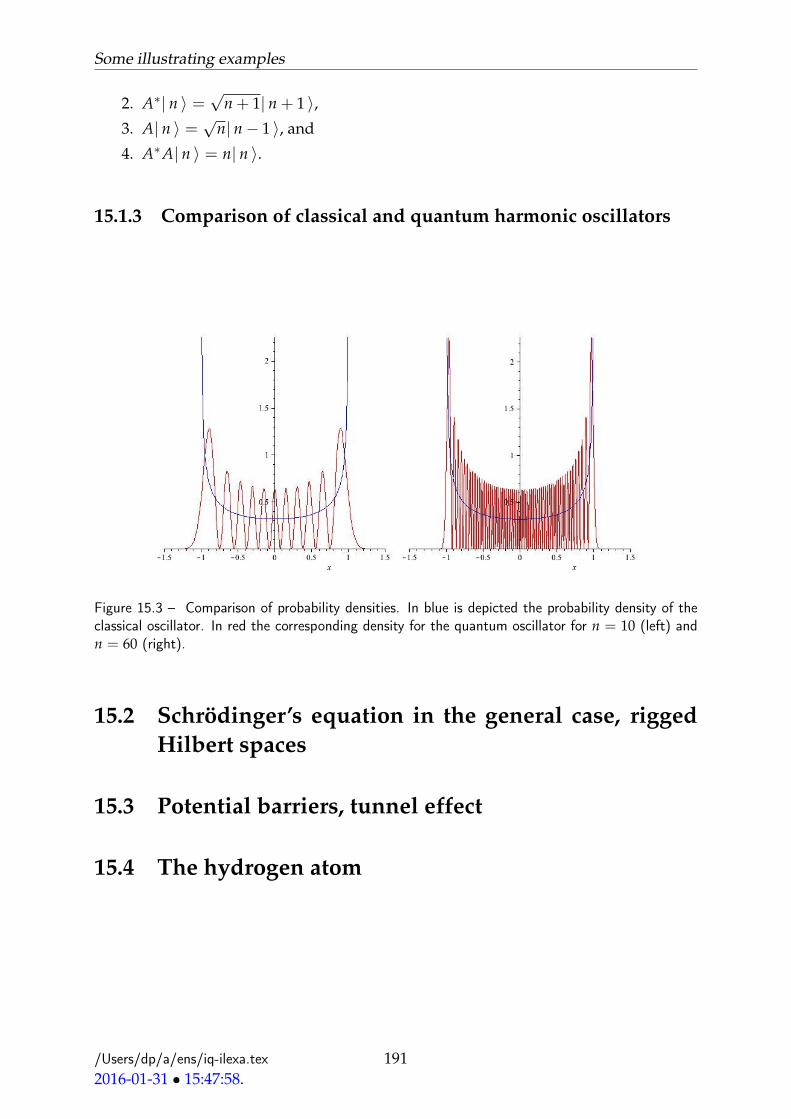
Some illustrating examples
2. A∗| n 〉 =√
n + 1| n + 1 〉,3. A| n 〉 =
√n| n− 1 〉, and
4. A∗A| n 〉 = n| n 〉.
15.1.3 Comparison of classical and quantum harmonic oscillators
Figure 15.3 – Comparison of probability densities. In blue is depicted the probability density of theclassical oscillator. In red the corresponding density for the quantum oscillator for n = 10 (left) andn = 60 (right).
15.2 Schrödinger’s equation in the general case, riggedHilbert spaces
15.3 Potential barriers, tunnel effect
15.4 The hydrogen atom
/Users/dp/a/ens/iq-ilexa.tex2016-01-31 • 15:47:58.
191

15.4. The hydrogen atom
Figure 15.4 – Comparison of distribution functions. In blue is depicted the distribution of the classicaloscillator. In red the corresponding distribution for the quantum oscillator for n = 1 (left), n = 10(middle), and n = 30 (right). Already for n = 30, the classical and quantum distributions are almostindistinguishable.
/Users/dp/a/ens/iq-ilexa.tex2016-01-31 • 15:47:58.
192

16Quantum formalism based on the
informational approach
Conditioning as disintegration [26], regular conditional probabilities, standardBorel spaces.
Projective limits [54]. Probabilities on lattices [50]. Effect algebras [37, 41].
193

/Users/dp/a/ens/iq-qinfo.tex2016-02-02 • 11:01:49.
194

17Quantifying information: classical and
quantum
17.1 Classical information, entropy, and irreversibility
The information content of a message is a probabilistic notion. The less probablea message is, the more information it carries. Let X be a random variable definedon (Ω,F , P) taking values in the finite set X = x1, . . . , xn Let PVn = p ∈ Rn
+ :∑n
i=1 pi = 1. To each element p ∈ PVn corresponds a probability measure PpX defined
by PpX(xi) = pi, for i = 1, . . . , n. Ask about the information content carried by the
random variable X is the same thing as trying to quantify the predictive power of thelaw PX. The main idea is that the information content of X is equal to the averageinformation missing in order to decide the outcome value of X when the only thing weknow is its law PX. Some reasonable requirements on the information content of X aregiven below:
— Suppose that all pi, i = 1, . . . , n but one are 0 and pj = 1, for some j. ThenP
pX(xj) = 1 and no information is missing, there is no uncertainty about the
possible outcome of X;— Suppose on the contrary that pi = 1/n, i = 1, . . . , n. Our perplexity is maximal
and this perplexity increases with n.— If S is to be interpreted as a missing information associated with a probability
vector p ∈ PVn, on denoting PV = ∪n∈NPVn, the function S : PV → R+ andthe first statement implies that S(1, 0, 0, . . . , 0) = 0 while S(1/n, . . . , 1/n) is anincreasing function of n.
— The function S must be invariant under permutations of its arguments i.e. S(pσ(1), . . . , pσ(n)) =
S(p1, . . . , pn) for all the permutations σ ∈ Sn.— If we split the possible outcome values into two sets, the function S must verify
195
17.1. Classical information, entropy, and irreversibility
the grouping property, i.e.
S(p1, . . . , pn; pn+1, . . . , pN) = S(qA, qB)
+qAS(p1
qA, . . . ,
pn
qA)
+qBS(pn+1
qB, . . . ,
pN
qB),
where qA = p1 + . . . + pn and qB = pn+1 + . . . + pN.— Finally, we require S(p1, . . . , pn; 0, . . . , 0) = S(p1, . . . , pn).
Theorem 17.1.1. The only function S : PV → R+ satisfying the above requirements is thefunction defined by
PV 3 (p1, . . . , pn) 7→ S(p1, . . . , pn) = −kn
∑i=1
pi log pi,
where k is an arbitrary non-negative constant and the convention 0 log 0 = 0 is used. Thefunction S is called the (classical) entropyf the probability vector.
Proof: To be filledlater.To be filledlater.
[17]
Entropy is closely related to irreversibility since the second principle of thermo-dynamics states: Entropy of an isolated system is a non decreasing function of time. It canremain constant only for reversible evolutions. For a system A undergoing an irreversibletransformation the entropy increases; however the system can be considered as partof a larger isolated composite system (A and environment), undergoing globally a re-versible transformation. In that case the total entropy (of the system A and of theenvironment) remains constant but since the entropy of A must increase, the entropyof the environment must decrease 1 hence the missing information decreases. In otherwords, when the system A undergoes an irreversible transformation, the environmentgains information.
This leads to the Landauer’s principle: When a computer erases a single bit of informa-tion, the environment gains at least k ln 2 units of information, where k > 0 is a constant.
1. Notice that this assertion is not in contradiction with the second principle of thermodynamicsbecause the environment is not isolated.
/Users/dp/a/ens/iq-qinfo.tex2016-02-02 • 11:01:49.
196

AWhat is light?
Nowadays light plays a key role in the transmission, storage, processing, and pro-tection of digital information (let it be classical or quantum); it is therefore importantfor practitioners of cryptography and digital communication to know some basic factsabout nature of light and its properties.
A.1 History
The conjectured nature of light has undergone several profound changes duringcenturies.
Ancient times. For the ancient Greek (ca. 4 century before our era) sight was aninteraction of light rays emitted both by the eye and the luminous source; rayswere supposed to travel in straight lines. For the ancient Indians (ca. 1–2 centuryof our era), light was a stream of high velocity “fire” atoms.
Early 17th century: Light is particles. René Descartes (1596–1650) explained refrac-tion (change of the direction of propagation when light crosses an interface oftwo different optical media, e.g. air-water) of light by a modification of its speedin the two media 1. Pierre Gassendi (1592–1655) proposed a particle theory oflight which has been later adopted by Sir Isaac Newton.
Late 17th–19th centuries: Light is waves. Christiaan Huygens (1629-1695) pro-posed a wave theory of light and introduced the fallacious idea of the luminif-erous ether as the medium into which light propagates.Leonhard Euler and Augustin-Jean Fresnel independently developed a consis-tent wave theory of light explaining many observed experimental facts. The
1. Nowadays, we know that speed of light changes when it changes medium of propagation but totravel slower in the denser medium, contrary to what Descartes conjectured.
197

A.2. Classical description
wave description culminated with the theory of electromagnetic radiation ofJames Clerk Maxwell who considered light as a very specific subset of all pos-sible electromagnetic waves providing a coherent classical theory that is stillinstrumental for the description of electromagnetic radiation of frequencies lessthan 1THz or for some specific phenomena concerning light in frequencies evenin the region of visible light.
1900 and onwards: Light is quantum relativistic particles. Monochromatic lightbeams in vacuum are streams of a very large number of elementary particlesof zero mass, the photons, travelling at the . . . speed of light c in all inertialframes. Every individual photon interacts (moderately) with matter particlesand the result of such interactions is described probabilistically. The photon-photon interaction can be safely omitted in all the phenomena described in thiscourse.
A.2 Classical description
In this appendix, we use the term “light” in a very broad sense, meaning electro-magnetic radiation of every frequency. Electromagnetic phenomena are described byMaxwell equations, connecting time and space derivatives of electric (E) and magneticfields (B) with charge (ρ) and current (J) densities. The parameters ε0 and µ0 are phys-ical constants.
∇ · E =ρ
ε0; ∇× E = −∂B
∂t
∇ · B = 0 ; ∇× B = µ0(J + ε0∂E∂t
)
z
E
Bk
Figure A.1 – The planes of oscillation of electric (red, E) and magnetic (blue, B) fields are mutuallyperpendicular and intersect at the axis of propagation of the electromagnetic wave, determined bythe Poynting’s pointing vector k = E×B
‖E‖‖B‖ . We call classical transversal polarisation the plane ofoscillation of the electric field. For instance, the wave depicted above has vertical polarisation.
In vacuum densities of charge and current vanish (ρ = 0, J = 0) and on denotingc−2 = ε0µ0, Maxwell equations admit wave solutions
E(x, t) = Emax sin(2π(z− ct)/λ))a(α); B(x, t) =1c
ez ∧ E(x, t),
/Users/dp/a/ens/iq-appen.tex2016-02-02 • 12:08:53.
198
What is light?
where a(α) =
cos αsin α
0
, is the polaristion vector, perpendicular to the vector k =
E∧B‖E‖‖B‖ is the vector of Poynting, pointing 2 in the direction of propagation. The planespanned by a and k is the plane of oscillation of the electric field. The magnetic fieldoscillates perpendicularly to E (see figure A.1). The distance between two maxima ofthe amplitude of the electric field (the distance travelled by the wave during its periodof oscillation) is called wavelength and is denoted by λ in the above equation. Thephysical constants ε0 and µ0 are such that c is the speed of light. The inverse of theperiod is called frequency of the wave.
Electromagnetic radiation arises at very different frequencies. The frequency of thewave (hence its wavelength) determines the colour of the light. The figure A.2 givesinformation about frequencies and wavelengths of different types of radiation and lo-cates the region of the visible spectrum in the whole frequency range of electromag-netic radiation.
Classically, electromagnetic radiation is produced by the electric dipole oscillationsinside antennas or atoms. The polarisation of light is hence determined by the axisof the emitting antenna or of the electric atomic dipole. While the orientation of anantenna is usually kept fixed, atoms are in all possible orientations in matter. Hence thelight produced by the Sun (or by incandescent bulbs) for instance arises in all possiblepolarisations; the corresponding electromagnetic wave comes as a superposition of allpossible waves of different polarisations (unpolarised light).
A.3 Simplified quantum descriprtion
Quantum mechanically, light is a flow of elementary particles called photons. Everyphoton has an energy (hence frequency) and is somehow localised in space, contraryto classical electromagnetic waves that propagate unboundedly. It is useful, althoughstrictly speaking wrong, to think of photons as small wave packets of given (approx-imately defined) frequency (see figure A.3). Beyond frequency, photons have anothercharacteristic called polarisation 3. If we are interested only to polarisation degree offreedom of a photon, the pure state describing its polarisation (see exercise ??) is givenby a ray ψ ∈H = C2. Denoting ε0 and ε1 the canonical basis of H, the general form ofψ is parametrized by two angles α, β:
ψ =
(cos(α)
exp(iβ) sin(α)
).
White light, as the one reaching us from the Sun, has a precise mixture of photonsof various frequencies. Monochromatic light, as the one emitted by a laser for instance,
2. This vector has been in introduced by the British physicist John Henry . . . Poynting.3. Photons are 0 mass particles, therefore in all frames they travel at the speed of . . . light c. Strictly
speaking, polarisation cannot be defined for particles not possessing a rest frame, only a relativisticquantity called helicity can be defined for them. Nevertheless, for the purpose of this course, we admitthat polarisation exists for photons as a quantum degree of freedom generalising classical polarisation.
/Users/dp/a/ens/iq-appen.tex2016-02-02 • 12:08:53.
199

A.4. Quantum optics
Figure A.2 – Spectrum of visible light occupies only a tiny portion of the frequency range of electro-magnetic radiation. (Source: Wikipedia).
has photons of a single frequency. When the light intensity is 1mW/cm2, every squarecentimetre 4 receives 3.59× 10²⁰ red light photons/s and roughly half as much violetphotons (ν = 700THz). Huge numbers of photons being involved even for modest in-tensities, the appropriate method to study experimental results is through a statisticaltreatment of measurements.
A.4 Quantum optics
4. Red light has a median frequency of ν = 420THz. A single red photon carries an energy E =2πhν = 2π × 1.05457× 10−34Js× 4.2× 1014s−1 = 2.783× 10⁻¹⁸J.
/Users/dp/a/ens/iq-appen.tex2016-02-02 • 12:08:53.
200

What is light?
Figure A.3 – A non totally rigorous but useful mental representation of a photon as a wave packet.The envelope (dashed blue curve) gives an estimate of the“position” of the photon (at the centre ofthe enveloping curve) and of its “frequency” as the number of times the enveloped wave (solid redcurve) changes sign per unit time. Position and frequency are determined only up to the precisionallowed by Heisenberg’s uncertainty principle. The direction of propagation of the depicted photon isthe horizontal axis, its polarisation is vertical.
/Users/dp/a/ens/iq-appen.tex2016-02-02 • 12:08:53.
201

A.4. Quantum optics
/Users/dp/a/ens/iq.tex2018-01-20 • 17:20:00.
202

Bibliography
[1] B. P. Abbott et al. Observation of gravitational waves from a binary black holemerger. Phys. Rev. Lett., 116:061102, Feb 2016. 7
[2] LM Adleman. Molecular computation of solutions to combinatorial problems.Science, 266(5187):1021–1024, 1994. 13
[3] N. I. Akhiezer and I. M. Glazman. Theory of linear operators in Hilbert space. DoverPublications Inc., New York, 1993. Translated from the Russian and with a pref-ace by Merlynd Nestell, Reprint of the 1961 and 1963 translations, Two volumesbound as one. 51, 55
[4] William Arveson. A short course on spectral theory, volume 209 of Graduate Texts inMathematics. Springer-Verlag, New York, 2002. 144, 148, 153
[5] R. S. Aspden, M. J. Padgett, and G. C. Spalding. Video recording true single-photon double-slit interference. ArXiv e-prints, February 2016. 37
[6] Alain Aspect, Jean Dalibard, and Gérard Roger. Experimental test of Bell’s in-equalities using time-varying analyzers. Phys. Rev. Lett., 49:1804–1807, Dec 1982.41, 43
[7] Alain Aspect, Philippe Grangier, and Gérard Roger. Experimental tests of realisticlocal theories via Bell’s theorem. Phys. Rev. Lett., 47:460–463, Aug 1981. 41
[8] Alain Aspect, Philippe Grangier, and Gérard Roger. Experimental realization ofEinstein-Podolsky-Rosen-Bohm Gedankenexperiment: A new violation of Bell’s in-equalities. Phys. Rev. Lett., 49:91–94, Jul 1982. 41, 43
[9] Francisco M. Assis, Aleksandar Stojanovic, Paulo Mateus, and Yasser Omar. Im-proving classical authentication over a quantum channel. Entropy, 14(12):2531–2549, 2012. 102
[10] Alexia Auffèves and Philippe Grangier. Contexts, systems and modalities: a newontology for quantum mechanics. Found. Phys., 46(2):121–137, 2016. 13
[11] Guido Bacciagaluppi and Antony Valentini. Quantum theory at the crossroads. Cam-bridge University Press, Cambridge, 2009. Reconsidering the 1927 Solvay Confer-ence, Translation of the proceedings, with a historical introduction and commen-tary. 46
[12] H. Barnum, C. Crepeau, D. Gottesman, A. Smith, and A. Tapp. Authentication ofquantum messages. In Foundations of Computer Science, 2002. Proceedings. The 43rdAnnual IEEE Symposium on, pages 449–458, 2002. 102
[13] David Beckman, Amalavoyal N. Chari, Srikrishna Devabhaktuni, and JohnPreskill. Efficient networks for quantum factoring. Phys. Rev. A (3), 54(2):1034–1063, 1996. 135
203

References
[14] J. S. Bell. Speakable and unspeakable in quantum mechanics. Cambridge UniversityPress, Cambridge, 2004. Collected papers on quantum philosophy. 15, 40
[15] John S. Bell. On the problem of hidden variables in quantum mechanics. Rev.Modern Phys., 38:447–452, 1966. 40
[16] John S. Bell. Bertlmann’s socks and nature of reality. Technical Report CERN-TH-2926, CERN, 1980. CERN Library. 83
[17] Fabio Benatti. Dynamics, information and complexity in quantum systems. Theoreticaland Mathematical Physics. Springer, Berlin, 2009. 196
[18] C. H. Bennett and G. Brassard. Quantum public key distribution system. IBMTechnical disclosure bulletin, 28:3153–3163, 1985. 93
[19] Charles H. Bennett. Quantum cryptography using any two nonorthogonal states.Phys. Rev. Lett., 68(21):3121–3124, 1992. 96
[20] A. S. Besicovitch. Almost periodic functions. Dover Publications, Inc., New York,1955. 55
[21] David Bohm. A suggested interpretation of the quantum theory in terms of "hid-den" variables. I. Phys. Rev., 85:166–179, Jan 1952. 40
[22] David Bohm. A suggested interpretation of the quantum theory in terms of "hid-den" variables. II. Phys. Rev., 85:180–193, Jan 1952. 40
[23] Harald Bohr. Almost periodic functions. Chelsea Publishing Company, New York,N.Y., 1947. 55
[24] Haïm Brezis. Analyse fonctionnelle. Collection Mathématiques Appliquées pour laMaîtrise. [Collection of Applied Mathematics for the Master’s Degree]. Masson,Paris, 1983. Théorie et applications. [Theory and applications]. 57
[25] Jerome R. Busemeyer and Peter D. Bruza. Quantum models of cognition and decision.Cambridge University Press, Cambridge, 2012. 13
[26] J. T. Chang and D. Pollard. Conditioning as disintegration. Statist. Neerlandica,51(3):287–317, 1997. 193
[27] Giulio Chiribella, Giacomo Mauro D’Ariano, and Paolo Perinotti. Theoreticalframework for quantum networks. Phys. Rev. A (3), 80(2):022339, 20, 2009. 45
[28] Giulio Chiribella, Giacomo Mauro D’Ariano, and Paolo Perinotti. Informationalderivation of quantum theory. Phys. Rev. A, 84:012311, Jul 2011. 45
[29] N. S. Dattani and N. Bryans. Quantum factorization of 56153 with only 4 qubits.ArXiv e-prints, November 2014. 135
[30] E. B. Davies and J. T. Lewis. An operational approach to quantum probability.Comm. Math. Phys., 17:239–260, 1970. 45
[31] Michel Demazure. Cours d’algèbre. Nouvelle Bibliothèque Mathématique [NewMathematics Library], 1. Cassini, Paris, 1997. Primalité. Divisibilité. Codes. [Pri-mality. Divisibility. Codes]. 91
[32] A. Einstein, B. Podolsky, and N. Rosen. Can quantum-mechanical description ofphysical reality be considered complete? Phys. Rev., 47:777–780, May 1935. 39
[33] Artur K. Ekert. Quantum cryptography based on bell’s theorem. Phys. Rev. Lett.,67:661–663, Aug 1991. 96
/Users/dp/a/ens/iq.bbl2018-01-20 • 17:21:57.
204

BIBLIOGRAPHY
[34] Richard P. Feynman, Robert B. Leighton, and Matthew Sands. The Feynman lec-tures on physics. Vol. 3: Quantum mechanics. Addison-Wesley Publishing Co., Inc.,Reading, Mass.-London, 1964. The new millenium edition, published by BasicBooks. 36
[35] Nicolas Gisin, Grégoire Ribordy, Wolfgang Tittel, and Hugo Zbinden. Quantumcryptography. Rev. Mod. Phys., 74:145–195, Mar 2002. 50
[36] Jonathan S. Golan. The linear algebra a beginning graduate student ought to know.Springer, Dordrecht, third edition, 2012. 62
[37] Teiko Heinosaari and Mário Ziman. The mathematical language of quantum theory.Cambridge University Press, Cambridge, 2012. From uncertainty to entangle-ment. 193
[38] B. Hensen et al. Loophole-free bell inequality violation using electron spins sep-arated by 1.3 kilometres. Nature, 526(7575):682–686, 2015. Supplementary infor-mation. 85
[39] Anthony J.G. Hey. Feynman and computation. Perseus Books Publishing, 1998. 45
[40] John K. Hunter and Bruno Nachtergaele. Applied analysis. World Scientific Pub-lishing Co. Inc., River Edge, NJ, 2001. 51, 53
[41] Peter Janotta and Haye Hinrichsen. Generalized probability theories: what de-termines the structure of quantum theory? J. Phys. A, 47(32):323001, 32, 2014.193
[42] Richard V. Kadison and John R. Ringrose. Fundamentals of the theory of operator alge-bras. Vol. I, volume 15 of Graduate Studies in Mathematics. American MathematicalSociety, Providence, RI, 1997a. Elementary theory, Reprint of the 1983 original. 68,145
[43] Alexander S. Kechris. Classical descriptive set theory, volume 156 of Graduate Textsin Mathematics. Springer-Verlag, New York, 1995. 33
[44] Andrei Nikolaevich Kolmogorov. Foundations of the theory of probability. ChelseaPublishing Co., New York, 1956. Translation edited by Nathan Morrison of theoriginal Grundbegriffe der Wahrscheinlichkeitsrechnung published in 1933, with anadded bibliography by A. T. Bharucha-Reid. 18
[45] Franck Laloë. Commentaires sur le paradoxe EPR, Septembre 2010.https://www.bibnum.education.fr/physique/physique-quantique/le-paradoxe-epr. 83
[46] Serge Lang. Introduction to Diophantine approximations. Springer-Verlag, New York,second edition, 1995. 130
[47] A. K. Lenstra and H. W. Lenstra, Jr. Algorithms in number theory. In Handbook oftheoretical computer science, Vol. A, pages 673–715. Elsevier, Amsterdam, 1990. 10,92
[48] A. K. Lenstra and H. W. Lenstra, Jr., editors. The development of the number fieldsieve, volume 1554 of Lecture Notes in Mathematics. Springer-Verlag, Berlin, 1993.11
[49] Arjen K. Lenstra. Integer factoring. Des. Codes Cryptogr., 19(2-3):101–128, 2000.Towards a quarter-century of public key cryptography. 92
/Users/dp/a/ens/iq.bbl2018-01-20 • 17:21:57.
205

References
[50] L. H. Loomis. The lattice theoretic background of the dimension theory of opera-tor algebras. Mem. Amer. Math. Soc., 1955(18):36, 1955. 164, 193
[51] H. Maassen. Quantum probability and quantum information theory. In Quan-tum information, computation and cryptography, volume 808 of Lecture Notes in Phys.,pages 65–108. Springer, Berlin, 2010. 41, 43, 44
[52] A. Manju and M. J. Nigam. Applications of quantum inspired computationalintelligence: a survey. Artificial Intelligence Review, 42(1):79–156, 2014. 13
[53] Enrique Martín-López, Anthony Laing, Thomas Lawson, Roberto Alvarez, Xiao-Qi Zhou, and Jeremy L. O’Brien. Experimental realization of Shor’s quantumfactoring algorithm using qubit recycling. Nature Photonics, 6, 10 2012. 113, 135
[54] Michel Métivier. Limites projectives de mesures. Martingales. Applications. Ann.Mat. Pura Appl. (4), 63:225–352, 1963. 193
[55] Michael A. Nielsen and Isaac L. Chuang. Quantum computation and quantum infor-mation. Cambridge University Press, Cambridge, 2000. 133
[56] Masanao Ozawa. An operational approach to quantum state reduction. Ann.Physics, 259(1):121–137, 1997. 45
[57] C. Pacher, A. Abidin, T. Lorünser, M. Peev, R. Ursin, A. Zeilinger, and J-A. Larsson.Attacks on quantum key distribution protocols that employ non-ITS authentica-tion, 2012. 102
[58] Juha-Pekka Pellonpää. Quantum instruments: I. Extreme instruments. J. Phys. A,46(2):025302, 16, 2013. 45
[59] Juha-Pekka Pellonpää. Quantum instruments: II. Measurement theory. J. Phys. A,46(2):025303, 15, 2013. 45
[60] Dimitri Petritis. Markov chains on measurable spaces, 2015. Premiminary draftof lecture notes taught at the University of Rennes 1. 45
[61] Dimitri Petritis. Théorie de la complexité, 2015. Notes de cours pour le master decryptographie - version préliminaire, Université de Rennes 1. 18, 79
[62] Dimitri Petritis. Probabilités pour la thórie de l’information, 2017. Notes de courspour le master de cryptographie - version préliminaire, Université de Rennes 1.18, 98
[63] Miklós Rédei. Why John von Neumann did not like the Hilbert space formalismof quantum mechanics (and what he liked instead). Stud. Hist. Philos. Sci. B Stud.Hist. Philos. Modern Phys., 27(4):493–510 (1997), 1996. 45
[64] Michael Reed and Barry Simon. Methods of modern mathematical physics. I. Func-tional analysis. Academic Press, New York, 1972. 51, 68
[65] R. L. Rivest, A. Shamir, and L. Adleman. A method for obtaining digital signaturesand public-key cryptosystems. Comm. ACM, 21(2):120–126, 1978. 11, 91
[66] Carlo Rovelli and Francesca Vidotto. Covariant Loop Quantum Gravity: An Elemen-tary Introduction to Quantum Gravity and Spinfoam Theory. Cambridge Monographson Mathematical Physics. Cambridge University Press, 1 edition, 2014. 14
[67] Walter Rudin. Real and complex analysis. McGraw-Hill Book Co., New York, thirdedition, 1987. 51
[68] Walter Rudin. Functional analysis. International Series in Pure and Applied Math-ematics. McGraw-Hill Inc., New York, second edition, 1991. 144
/Users/dp/a/ens/iq.bbl2018-01-20 • 17:21:57.
206

BIBLIOGRAPHY
[69] Raymond A. Ryan. Introduction to tensor products of Banach spaces. Springer Mono-graphs in Mathematics. Springer-Verlag London Ltd., London, 2002. 68
[70] Erwin Schrödinger. Discussion of probability relations between separated sys-tems. Mathematical Proceedings of the Cambridge Philosophical Society, 31:555–563, 101935. 40
[71] Erwin Schrödinger and Paul Adrien Maurice Dirac. Probability relations betweenseparated systems. Mathematical Proceedings of the Cambridge Philosophical Society,32:446–452, 10 1936. 40
[72] Denis Serre. Matrices, volume 216 of Graduate Texts in Mathematics. Springer-Verlag, New York, 2010. Theory and applications, 2nd edition, Translated fromthe 2001 French original. 80
[73] Claude Shannon. Communication theory of secrecy systems. Bell System TechnicalJournal, 28:656–715, 1949. 90
[74] Peter W. Shor. Polynomial-time algorithms for prime factorization and discretelogarithms on a quantum computer. SIAM J. Comput., 26(5):1484–1509, 1997. 10,11, 89
[75] Thomas Sierocinski, Nathalie Th’eret, and Dimitri Petritis. Fuzzy and quantummethods of information retrieval to analyse genomic data from patients at differ-ent stages of fibrosis. In 2008 First International Symposium on Applied Sciences onBiomedical and Communication Technologies, pages 1–5, Oct 2008. 13
[76] Instituts Solvay. La structure de la matière: Rapports et discussions du Conseil dephysique tenu à Bruxelles du 27 au 31 octobre 1913. Gauthier-Villars, Paris, 1921.46
[77] Instituts Solvay. La structure de la matière: Rapports et discussions du Conseil dephysique tenu à Bruxelles du 29 au 29 octobre 1933. Gauthier-Villars, Paris, 1934.46
[78] Instituts Solvay, Maurice de Broglie, Paul Langevin, and Ernest Solvay. La théoriedu rayonnement et les quanta: Rapports et discussions de la réunion tenue à Bruxelles,du 30 Octobre au 3 Novembre 1911, sous les auspices de E. Solvay. Gauthier-Villars,Paris, 1912. 46
[79] V. A. Uspenskiı, A. L. Semenov, and A. Kh. Shen’. Can an (individual) sequenceof zeros and ones be random? Uspekhi Mat. Nauk, 45(1(271)):105–162, 222, 1990.18
[80] C. J. van Rijsbergen. The geometry of information retrieval. Cambridge UniversityPress, Cambridge, 2004. 13
[81] V. S. Varadarajan. Geometry of quantum theory. Springer-Verlag, New York, secondedition, 1985. Reprint of the original edition published in two volumes, volume Iin 1968 and volume 2 in 1970. 45, 164, 179
[82] Gilbert S. Vernam. Cipher printing telegraph systems for secret wire and radio tele-graphic communications, volume 55. 1926. 90
[83] J. von Neumann. Über einen Satz von Herrn M. H. Stone. Ann. of Math. (2),33(3):567–573, 1932. 16
[84] Johann von Neumann. Mathematische Grundlagen der Quantenmechanik. Unverän-derter Nachdruck der ersten Auflage von 1932. Die Grundlehren der mathematis-chen Wissenschaften, Band 38. Springer-Verlag, Berlin, 1968. 45
/Users/dp/a/ens/iq.bbl2018-01-20 • 17:21:57.
207

Index of terms and notions
[85] Joachim Weidmann. Linear operators in Hilbert spaces, volume 68 of Graduate Textsin Mathematics. Springer-Verlag, New York, 1980. Translated from the German byJoseph Szücs. 52, 53, 68
[86] Nanyang Xu, Jing Zhu, Dawei Lu, Xianyi Zhou, Xinhua Peng, and Jiangfeng Du.Quantum factorization of 143 on a dipolar-coupling nuclear magnetic resonancesystem. Phys. Rev. Lett., 108:130501, Mar 2012. 135
[87] Nicholas Young. An introduction to Hilbert space. Cambridge Mathematical Text-books. Cambridge University Press, Cambridge, 1988. 51
/Users/dp/a/ens/iq.tex2018-01-20 • 17:20:00.
208

BIBLIOGRAPHY
Index of symbols
/Users/dp/a/ens/iq.tex2018-01-20 • 17:20:00.
209

Index of terms and notions
Index of terms and notions
algebra, 140Banach, 140Boolean, 162Boolean σ-, 163commutative, 140C∗, 142normal element of an, 140normed, 140self-adjoint element of an, 140unital, 140unitary element of an, 140
algebraicadjoint, 140isometry, 140
algorithmMonte Carlo, 107
automorphismconvex, 173
Banach algebrageneral linear group of invertible el-
ements of, 151invertible element of, 151
Boolean circuit, 108
complement, 162completion, 53complexity class, 106
BPP, 107NP, 106P, 106PSPACE, 106
computable function, 105computational
space, 106time, 106
computational history, 105computational path, 105conditional expectation
classical, 54
density matrix, 178determinant, 148direct sum, 56dual
algebraic, 57
dual spacetopological, 57
effect, 28classical (unsharp), 28sharp classical, 27
eigenvalue, 150entanglement, 79equation
Hamilton, 184Schroedinger, 188
Euler function, 90expected value, 169
familycomplete, 55
gateFreidkin, 110
harmonic oscillatorclassical, 183quantum, 187
Hasse diagram, 162hatling flag, 111Hilbert
norm, 52
inequalityCauchy-Schwarz-Buniakovski, 52
inequaltiyBessel, 55
involution, 140isometry, 144
partial, 144
joint probability distribution, 172
language, 105lattice, 162
atom (in a), 163atomic, 163automorphism, 164complemented, 162Dilworth, 163distributive, 162isomorphism, 164modular, 163
/Users/dp/a/ens/iq.tex2018-01-20 • 17:20:00.
210

BIBLIOGRAPHY
of propositions, 161orthocomplemented, 165orthomodular, 163σ-complete, 163
linearfunctional, 57
linear span, 53closed, 53
logic, 165classical, 165probability measure on, 168standard quantum, 166state on, 168
marginalquantum, 73
measurement, 15classical, 33quantum, 46
momentum operator, 157
observable, 15associated with a logic, 166bounded, 166classical, 164classical (unsharp), 29classical sharp, 33constant, 166discrete, 166quantum, 46sharp classical, 27spectral value of, 166spectrum of, 166strict value of an, 166
operator, 58adjoint, 59, 157annihilation, 189bounded, 58closable, 157closed, 157closure, 157creation, 189densely defined, 157density, 72, 178diagonalisable, 153extension of an, 157graph of, 157Hermitean, 143invertible, 59, 149, 157
isometric, 144kernel of, 58norm, 58normal, 60, 145orhoprojection, 143positive, 69, 143projection, 60, 143range of, 58restriction of an, 157self-adjoint, 60, 143skew-adjoint, 60trace class, 71trace-class, 177unbounded, 157unitary, 60, 144von Neumann, 178
orthocomplementation, 165orthogonal
complement, 56orthoprojections, 143subsets, 56vectors, 52, 56
orthoprojection, 61, 143
partial isometry, 144partial trace, 72partially ordered set, 161phase space
classical, 31quantum, 45, 46
Poisson bracket, 186polynomial growth, 106poset, 161position operator, 157predicate, 105predicate:decidable, 105probability
extremal, 31probability distribution, 169projection, 60, 143proposition
simultaneously verifiable, 171
qubit, 46question, 28, 33, 167
associated with proposition, 167
random variable, 18law of, 19
/Users/dp/a/ens/iq.tex2018-01-20 • 17:20:00.
211

Index of terms and notions
ray, 176reducibility of classical randomness, 33representation
faithful, 145of locally compact group, 173space, 145∗, 145unitarily equivalent, 145
resolution of identity, 28resolvent
set, 149
scalar product, 52Schmidt
decomposition, 80rank, 80vector, 80
self-dual, 58sequence
Cauchy, 52fundamental, 52
setclosed, 52convex, 54
simultaneous observability, 171space
Banach, 52complete, 52Hilbert, 52metric, 52normed, 52pre-Hilbert, 52
spectralmeasure, 154radius, 152
spectral projection, 28spectrum, 149, 151
continuous, 150point, 150residual, 150
∗-algebra, 140∗-homomorphism, 140state
classical, 33classically correlated, 81entangled, 81function, 167pure, 169superposition, 170
tracial, 179uncorrelated, 81
stochastickernel, 19
symmetry, 179
tensor, 65entangled, 65factored, 65simple, 65
tensor productalgebraic, 64universality property, 63
theoremGel’fand-Naïmark, 145Gleason, 179Liouville, 187of spectral decomposition, 155
time evolutionclassical, 33quantum, 46
trace, 71, 176partial, 72
Turing machinedeterministic, 104non-deterministic, 106pre-quantum, 110probabilistic, 107quantum, 111
variance, 169vector
entagled, 79vector space
free, 64
/Users/dp/a/ens/iq.tex2018-01-20 • 17:20:00.
212