mathematical foundations of quantum mechanics 2016 … · mathematical foundations of quantum...
TRANSCRIPT

Mathematical Foundations of QuantumMechanics 2016-17
Dr Judith A. McGovern
Maths of Vector Spaces
This section is designed to be read in conjunction with chapter 1 of Shankar’s Principles ofQuantum Mechanics, which will be the principal course text book. Other on-line resources arelinked from the course home page.
Another source that covers most of the material at the right level is Griffiths’ Introduction toQuantum Mechanics, which has an appendix on linear algebra.
Riley’s Mathematical Methods for the Physical Sciences is available as an ebook, and chapter8 covers much of the material too. This is particularly recommended if Shankar seems initiallyintimidating. Unfortunately Riley does not use Dirac notation except for inner products, usingboldface a where we would use |a〉, but if you understand the concepts from that book, thenotation used here should not be a barrier. Some further comments on Riley’s notation can befound in section 1.4. Riley (or a similar text such as Boas) should be consulted for revision onfinding the eigenvalues and eigenvectors of matrices.
This outline omits proofs, but inserts the symbol P to indicate where they are missing. In theearly stages the proofs are extremely simple and largely consist of assuming the opposite anddemonstrating a contradiction with the rules of vector spaces or with previous results. Manyare in Shankar but some are left by him as exercises, though usually with hints. By the timewe get on the properties of operators (existence of inverses, orthogonality of eigenstates) someof the proofs are more involved. Some of the principal proofs are on the examples sheet. Proofsfrom this section are not examinable, but you are advised to tackle some of them to make sureyou understand the ideas.
1

1.1 Vector Spaces
DefinitionShankar pp 1-3, Riley 8.1, Griffiths A.1
A linear vector space is a set V of elements called vectors, |v〉, |w〉..., for whichI) An operation, “+”, is defined, which for any |v〉 and |w〉 specifies how to form |v〉+ |w〉II) Multiplication by a scalar is also defined, specifying α|v〉and these operations obey the following rules:
1. The result of these operations is another member of V (closure).
2. |v〉+ |w〉 = |w〉+ |v〉 (vector addition is commutative)
3. (|u〉+ |v〉) + |w〉 = |u〉+ (|v〉+ |w〉) (vector addition is associative)
4. α(β|v〉) = (αβ)|v〉 (scalar multiplication is associative)
5. 1 |v〉 = |v〉
6. α(|v〉+ |w〉) = α|v〉+ α|w〉 (distributive rule 1)
7. (α + β)|v〉 = α|v〉+ β|v〉 (distributive rule 2)
8. The null or zero vector is written as |0〉 (or often, just 0), with |0〉+ |v〉 = |v〉
9. For every vector |v〉 there is another, denoted |−v〉, such that |v〉+ |−v〉 = |0〉
Note in the definition of |−v〉 the minus sign is just part of the name of the inverse vector.
The zero vector is unique. 0|v〉 = |0〉 for any |v〉 P.The inverse is unique and given by |−v〉 = (−1)|v〉 P.We use “minus” in the following sense: |v〉 − |w〉 = |v〉+ (−1)|w〉 = |v〉+ |−w〉.If the scalars α, β... are complex (written α, β ∈ C), we have a complex vector space, otherwise(α, β ∈ R) we have a real one. If we want to distinguish we write V(C) and V(R), but if wedon’t specify we assume it is complex. (C or R is called the field of the space).
These rules just confirm what you do naturally, but:
• You should not assume anything about abstract vectors that is not given in the definition.
• The rules apply to many things apart from traditional “arrow” vectors.
• So far there is no concept of “angle” between vectors, nor any way to measure “length”.
Examples
• Ordinary 3D “arrow” vectors belong to a real vector space.1
1“arrow” vectors have length and direction in 3D, but they do not have a fixed starting point, so two vectorsare added by placing the tail of second at the tip of the first; multiplication by a scalar changes the length butnot the direction. In physics, displacement vectors are a better picture to keep in mind than positions.
• Real numbers form a (very simple) real vector space.
• The set RN (CN) of sequences of N real (complex) numbers, such as |c〉 = (c1, c2, . . . cN)form a real (complex) vector space, where ‘+’ is ordinary matrix addition, |0〉 = (0, 0, . . . 0)and the inverse is |−c〉 = (−c1,−c2, . . .− cN).
• The set of all polynomials such as f(x) = a0 + a1x+ a2x2 + . . . , with ai ∈ C and x ∈ R,
forms a complex vector space; |0〉 is the polynomial with all coefficients ai equal to zero.
• The set of 2 × 2 complex matrices
(a bc d
), with a, b, c, d ∈ C, form a complex vector
space under matrix addition (in fact any such set of n×m matrices gives a vector space).
Ket NotationShankar p 3, Griffiths A.1
Here we are using the Dirac notation for vectors, with the object |v〉 also being called aket. The text between the “|” and the “〉” is just a name or label for the ket, which can takemany forms—we will see letters, numbers, symbols (|+〉, |♥〉), reminders of how the vector wasformed (|αv〉 for α|v〉).... Sensible choices of names can help make the algebra easy to follow.The notation prevents abstract vectors being confused with simple numbers.
1.2 Linear Independence, bases and dimensions
Linear IndependenceShankar p 4, Riley 8.1.1, Griffiths A.1
Since there are infinitely many scalars, all vector spaces have infinitely many members.
If from V we pick n vectors |x1〉, |x2〉, . . . , |xn〉, the set is said to be linearly dependent ifit is possible to write
∑ni=1 ai|xi〉 = |0〉 where the coefficients ai are not all zero. It follows that
at least one of the vectors can be written as a sum over the others P.
If this is not possible, the set is linearly independent. Any two non-parallel “arrow” vectorsare linearly independent; any three arrow vectors in a plane are linearly dependent.
Dimensions and BasesShankar pp 5-7, Riley 8.1.1, Griffiths A.1
A vector space has dimension N if it can accommodate a maximum of N linearly-independentvectors. It is infinite-dimensional if there is no maximum. We use VN if we want to specify thedimension.
A basis in a vector space V is a set |x1〉, |x2〉, . . . , |xN〉 ≡ |xi〉 of linearly-independentvectors such that every vector in V is a linear combination of the basis vectors |xi〉; that is, for

an arbitrary vector |v〉,
|v〉 =N∑i=1
vi|xi〉
where vi are suitable coefficients (or components or coordinates). For a given basis andvector |v〉, these components are unique P. However in different bases, a given vector will havedifferent components.
In general components are complex, but for a real vector space (with a suitable choice of basis)they are real.
Example: In real 3-D space, using the usual notation, the vectors i, j,k form a basis . (Thesemay also be written x, y, z or ex, ey, ez.) So does any other set of three non-coplanarvectors.
Every basis in VN has N elements; conversely any set of N linearly-independent vectors in VN
forms a basis P.
When we add vectors, the coordinates add: if |w〉 = α|u〉 + β|v〉, with |u〉 =∑ui|xi〉, |v〉 =∑
vi|xi〉 and |w〉 =∑wi|xi〉, then wi = αui + βvi
P.
Any set of at least N vectors which includes a basis as a subset is said to span the space;obviously a basis spans the space.
For convenience, we will often write a basis as |i〉 ≡ |1〉, |2〉, . . . |N〉. Recall that what iswritten inside the ket is just a label. Numbers-as-labels in kets will be widely used, so it isimportant to remember they have no other significance. |1〉+ |2〉 6= |3〉!
RepresentationsShankar pp 10-11, Riley 8.3, Griffiths A.1
For a given basis |xi〉, and a vector |v〉 =∑N
i=1 vi|xi〉, the list of components vi is a repre-sentation of the abstract vector |v〉. We write this as a vertical list (or column vector):
|v〉 −→x
( v1v2...vN
).
The symbol −→x
means “is represented by”, with the x being a name or label for the basis
(which will be omitted if the basis is obvious).
Note that in their own representation the basis vectors are simple:
|x1〉 −→x
(10...0
), |x2〉 −→
x
(01...0
), . . . |xN〉 −→
x
(00...1
).
If ui, vi and wi are the components of |u〉, |v〉 and |w〉 in this basis, and |w〉 = α|u〉+ β|v〉,
|w〉 −→x
αu1 + βv1
αu2 + βv2...
αuN + βvN

Hence all manipulations (addition, multiplication by a scalar) of the abstract vectors or ketsare mirrored in corresponding manipulations of the column vectors. A fancy way of saying thesame this is that all N -dimensional vector spaces are homomorphic to CN , and hence to oneanother. Practical calculations often start by specifying a basis and working with the corre-sponding representations of vectors in that basis. We will repeatedly find the same calculationsrecurring for physically different vector spaces that happen to have the same dimension.
If we have another basis, |yi〉, |v〉 will be represented by a different column vector in thisbasis, and the |xi〉 will have more than one non-zero component.
Example: given a 2D real vector space with a basis |x1〉, |x2〉 and another|y1〉 = |x1〉+|x2〉, |y2〉 = |x1〉−|x2〉, and |v〉 = 2|x1〉 + 3|x2〉 = 5
2|y1〉 − 1
2|y1〉, we have for
instance
|v〉 −→x
(23
), |v〉 −→
y
(5/2−1/2
), |y2〉 −→
x
(1−1
), |x1〉 −→
y
(1/21/2
).
Subspaces and direct sumsShankar pp 17-18
Given an N -D vector space VN , a subset of its elements that form a vector space amongthemselves is a subspace.
For examples in ordinary 3-D space:• all vectors along the x axis are a 1-D subspace: V1
x
• all vectors in the xy plane which includes the origin are a 2-D subspace: V2xy.
Note both of these contain the origin, and the inverse of any vector in the subspace.
Any n-D subset of a basis of VN will span a new subspace Vn P. Of course the space containsall linear combinations of these basis vectors, not just the vectors themselves.
Given two spaces, VNa and VM
b , (where a and b are just labels), their so-called direct sum,written VN
a ⊕ VMb is the set containing all elements of VN
i and VMj and all possible linear
combinations between them. This makes it closed, and so the direct sum is a new vector space.A set consisting of N basis vectors from VN
a and M from VMb forms a basis in VN
a ⊕VMb , which
is an N +M dimensional space. VNa and VM
b are subspaces of this space.
Example: V1x ⊕ V 1
y = V2xy. Bases for the two 1-D spaces are the 1-element sets i and j; so
i, j is a basis on their direct sum. V1x and V1
y are now subspaces of the new space V2xy. Note
that V2xy contains points off the x and y axes which are not in either of the component spaces,
but are produced by linear combinations (e.g. 2i− 10j).
Note that for this to work, the two spaces must have only the zero vector in common. Thedirect sum of the xy plane and the xz plane is not four-dimensional!
Product spacesShankar pp 248-249 (chapter 10)
A different way of combining two spaces is the “tensor direct product”, denoted VNa ⊗ VM
b .Though important in quantum mechanics, it is hard to come up with examples from classicalphysics. They arise when a system has two distinct aspects, both of which are vectors, and inorder to specify the state of the system both vectors have to be given.
If |ai〉 and |bi〉 are basis sets for the two spaces, one possible basis for the product space isformed by picking one from each—say the ith from the first set and the jth from the secondset. There are N ×M possibilities, so the product space has dimension N ×M . These statesare written |i, j〉 ≡ |ai〉⊗ |bj〉. The ⊗ is best regarded simply as a separator; it doesn’t indicateany operation that is carried out.
Note that for |p〉, |q〉 ∈ VNa and |v〉, |w〉 ∈ VM
b , while all vectors |p〉⊗|v〉 are in VNa ⊗VM
b , not allvectors in the product space can be written in this way. Those that can are called separable,i.e. they have a specified vector in each separate space. The vector α|p〉 ⊗ |v〉 + β|q〉 ⊗ |w〉is in the product state but is not separable unless |p〉 ∝ |q〉 or |v〉 ∝ |w〉.2 This is wherethe distinction between classical and quantum mechanics comes in. In quantum mechanics, anon-separable state is called an entangled state.
Linearity and associative and distributive laws hold, eg(α|p〉
)⊗(β|v〉+ γ|w〉
)= αβ
(|p〉 ⊗ |v〉
)+ αγ
(|p〉 ⊗ |w〉
)Note |v〉 ⊗ |0〉 and |0〉 ⊗ |w〉 are the same and equal to the null vector P.
1.3 Inner Products
DefinitionsShankar pp 7-9, Riley 8.1.2, Griffiths A.2
In applications in physics we usually want to define the length or “norm” of a vector, andthe “angle” between two vectors. To be precise, we define the inner product of |v〉 and |w〉,written 〈v|w〉, as a complex number that obeys three rules:
(I) 〈v|w〉 = 〈w|v〉∗. (Skew symmetry)
(II) 〈v|v〉 ≥ 0, with equality if and only if |v〉 is the zero vector. (Positive definiteness)
(III) 〈v|(α|u〉+β|w〉
)= α〈v|u〉+β〈v|w〉, where α, β ∈ C. (Linearity on the right or ket side).
A vector space with an inner product is called an inner-product space. The term Hilbertspace is also used; in finite-dimensional spaces at least they are equivalent for our purposes.
Examples• For real vectors in 3-D the usual scalar product satisfies these rules P.• So does the “sum of products” rule
∑i viwi for lists of real numbers (RN).
• However the “sum of products” rule does NOT work for lists of complex numbers (CN); but∑i v∗iwi does.
It follows that for vectors from a complex vector space, if |p〉 = α|u〉+ β|v〉,
〈p|w〉 = α∗〈u|w〉+ β∗〈v|w〉 :
i.e. inner products are “anti-linear” or “conjugate-linear” on the left P.
Two vectors are orthogonal if their inner product is zero: 〈v|w〉 = 0 = 〈w|v〉.We choose the norm or length of a vector |v〉 to be |v| =
√〈v|v〉. If |v| = 1, |v〉 is normalised.
2|p〉 ∝ |q〉 means that there is some scalar α such that |p〉 = α|q〉

Orthonormal basesShankar pp 9-12, 14-15, Riley 8.1.2, Griffiths A.2
A set of vectors in a vector space VN , |i〉 ≡ |1〉, |2〉, ...|n〉, all of unit norm, and all orthogonalto each other, is called an orthonormal set. By definition they satisfy 〈i|j〉 = δij (i.e. 1 ifi = j and 0 otherwise).
(We could equally have denoted the basis |xi〉. Especially if we are talking about vectors inreal 3D space we might use the notation |ei〉 instead.)
Vectors in an orthonormal set are linearly independent P, so n ≤ N .
If there are enough vectors in the orthonormal set to make a basis (for finite-dimensional spaces,n = N), we call it an orthonormal basis or complete orthonormal set.
Every [finite-dimensional] vector space has an orthonormal basis P (actually infinitely many).(This theorem is actually true even for infinite-dimensional vector spaces but the proof is hard.)
Coordinates in an orthonormal basis have very simple expressions: if |v〉 =∑
i vi|i〉, thenvi = 〈i|v〉 P.
If vi and wi, are the coordinates of |v〉 and |w〉 respectively, 〈v|w〉 =∑
i v∗iwi and 〈v|v〉 =∑
i v∗i vi =
∑i |vi|2 ≥ 0 P.
(Remember in proving these, you need to use different indices (“dummy indices”) for each sum,and these in turn must be different from any “free” index, which stands for any of 1 . . . N . Thusfor example 〈i|v〉 =
∑j vj〈i|j〉.)
Though coordinates are basis-dependent, the sums that give norms and inner products arebasis-independent, as will be shown later.
Gram-Schmidt orthogonalisation can be used to construct an orthonormal basis |i〉 froma set |vi〉 of N linearly-independent vectors. First, let |1〉 be |v1〉/|v1|. Then take |v2〉, subtractoff the component parallel to |1〉, and normalise:
|2〉 = C2
(|v2〉 − 〈1|v2〉|1〉
)where |C2|−2 = 〈v2|v2〉 − 〈v2|1〉〈1|v2〉
Continue taking the remaining |vj〉 in turn, subtract off the component parallel to each previ-ously constructed |i〉, normalise and call the result |j〉:
|j〉 = Cj
(|vj〉 −
j−1∑i=1
〈i|vj〉|i〉
)
where Cj is the normalisation constant. The resulting basis is not unique, because it dependson the ordering of the basis vectors, which is arbitrary; also the normalisation constants areonly defined up to a phase. (This construction proves the existence of an orthonormal basis,as asserted above.)
BrasShankar pp 11-14, Griffiths 3.6
In Dirac notation, the inner product 〈v|w〉 is considered as a bra 〈v| acting on ket |w〉 to forma (scalar) “bracket”. Another way of saying this is that a bra 〈v| is an object with the property

that it can be combined with any ket |w〉 from VN to give the inner product 〈v|w〉. For each ket,there is a corresponding bra and vice versa, so 〈w|v〉 = 〈v|w〉∗ will be the result of combiningthe bra 〈w| with the ket |v〉.Mathematically, if the ket lives in a vector space VN , then the bra is an element of anothervector space, called the dual of VN , but we will not need this distinction. (Students oftenstumble over the concept of bras when they first meet them, so the interpretation in terms ofrow vectors to be given below is a very useful picture.)
Given a basis |i〉, the corresponding bras 〈i| span the space of bras, and an arbitrary bracan be expanded 〈v| =
∑i v∗i 〈i|, with 〈v|i〉 = v∗i . Thus the coordinates of the bra 〈v| are v∗i
P.Note that if the ket |w〉 =
(α|u〉+ β|v〉
), the corresponding bra is 〈w| =
(α∗〈u|+ β∗〈v|
).
If we represent a ket |v〉 as a column matrix of coordinates v:
|v〉 →
v1
v2...vN
≡ v,
the corresponding bra is a row matrix:
〈v| → (v∗1, v∗2, . . . v
∗N) = (v>)∗ ≡ v†.
and the ordinary rules of matrix multiplication make the operation of a bra on a ket give asingle complex number:
〈v|w〉 → (v∗1, . . . v∗N)
w1...
wN
=N∑i=1
v∗iwi
just as before.
Note that the basis kets given by 〈1| → (1, 0, . . . , 0, 0) etc.
InequalitiesShankar pp 16-17, Riley 8.1.3, Griffiths A.2
The Schwarz Inequality: for any vectors |v〉, |w〉, |〈v|w〉| ≤ |v| |w| P.The equality holds only if |v〉 ∝ |w〉 P.Notice that the same rule applies to ordinary dot products, since | cos θ| ≤ 1.
The triangle inequality: If |w〉 = |u〉 ± |v〉, then |w| ≤ |u|+ |v| P.Notice that this holds for the lengths of ordinary “arrow” vectors that form a triangle! Bysymmetry, the result is cyclic, i.e. |v| ≤ |w|+ |u| etc.
Inner products in product spaces
Let |p〉, |q〉 ∈ Va and |v〉, |w〉 ∈ Vb, and let an inner product be defined on each space. Theinner product in the product space Va ⊗ Vb is defined as
(〈p| ⊗ 〈v|
)(|q〉 ⊗ |w〉
)= 〈p|q〉〈v|w〉,
which of course is a scalar.

If |pi〉 and |vi〉 are orthonormal bases in each space, then |pi〉 ⊗ |vj〉 is an orthonormalbasis in the product space (there are of course others, which need not be separable).
1.4 Operators
DefinitionShankar 18-20, Riley 8.2, 7.2.1, Griffiths A.3
Operators change kets into other kets in the same vector space:
A|v〉 = |w〉
For the moment we mark operators with a hat, .
Linear operators (we will not consider others) have the property that
A (α|v〉+ β|w〉) = αA|v〉+ βA|w〉 and(αA+ βB
)|v〉 = αA|v〉+ βB|v〉.
Hence any operator acting on the zero vector gives zero.The identity operator I leaves a ket unchanged: I|v〉 = |v〉.The product of two operators, say AB, means “apply B first and then apply A to theresult”. If B|v〉 = |u〉, AB|v〉 = A|u〉.A and B will not in general commute, in which case this is not the same as BA|v〉.If, for all kets in the space, BA|v〉 = |v〉, then B is called the inverse of A and denoted A−1.We can write A−1A = I. For finite dimensional spaces, AA−1 = I also P.
Not all operators have inverses. However if the equation A|v〉 = |0〉 has no solutions except|v〉 = |0〉, the inverse A−1 does exist P.
Inverse of matrix products: if C = AB, then C−1 = B−1A−1 P.
Identity and Projection operatorsShankar 22-24, (Riley 8.4), Griffiths 3.6
The object |a〉〈b| is in fact an operator since, acting on any ket |v〉, it gives another ket, 〈b|v〉|a〉.(Whatever |v〉 we choose, the resulting ket is always proportional to |a〉.) This is termed theouter product of |a〉 and |b〉, and is entirely distinct from the inner product 〈b|a〉, which is ascalar.
Using an orthonormal basis |i〉, we can define projection operators, Pi = |i〉〈i|, which“pull out” only the part of a vector |v〉 which is parallel to |i〉: Pi|v〉 = vi|i〉. The product oftwo projection operators is zero or equivalent to a single projection P: PiPj = δijPi.
These are examples of operators which do not have an inverse, since Pi|v〉 = 0 will be satisfiedfor many non-zero kets |v〉. The lack of an inverse reflects the fact that when we operate withPi on a vector, we lose all information about components orthogonal to |i〉, and no operatorcan restore it.
One very useful way of writing the identity operator is as follows P:
I =∑i
Pi =∑i
|i〉〈i|
This is called the completeness relation. The sum must be over projectors onto an orthonor-mal basis.

Matrix representation of operatorsShankar 20-22, 25, Riley 8.3, 7.3.1, Griffiths A.3
[Comment on notation in Riley: Riley uses boldface for abstract vectors where we use kets,and calligraphic letters without “hats” for operators: hence A|v〉 = |u〉 is written Av = u. Weuse boldface for column vectors and matrices of components, but Riley uses a sans-serif font,so Av = u is a matrix equation.]
We can form the inner product of |u〉 ≡ A|v〉 with another vector |w〉, to get 〈w|u〉 = 〈w|(A|v〉
).
This is called a matrix element of A, and is more often written 〈w|A|v〉.If we have an orthonormal basis |i〉, we can form all possible matrix elements of A betweenvectors of the basis, Aij = 〈i|A|j〉; these are the coordinates of A in this basis. Then P
A|v〉 =∑ij
Aijvj|i〉 and 〈w|A|v〉 =∑ij
w∗iAijvj.
The numbers Aij can be arranged in a matrix A, i labelling the row and j the column, whichgives
〈w|A|v〉 = (w∗1, w∗2, . . . w
∗N)
A11 A12 . . . A1N
A21 A22 . . . A2N...
......
......
...AN1 AN2 . . . ANN
v1
v2...
vN
= w†Av (1.1)
The ith column of matrix A is just the coordinates of |Ai〉 ≡ A|i〉, i.e. the transformed basisket.
If the determinant of A vanishes, its columns are not linearly independent. That means that|Ai〉 is not a basis, and the vectors |Av〉 belong to a lower-dimensional sub-space of VN .Hence det A = 0 means that A−1 does not exist.
The matrix elements of the product of two operators can be found by inserting the completenessrelation
∑k |k〉〈k| as an identity operator in AB = AIB:
(AB)ij = 〈i|AB|j〉 =∑k
〈i|A|k〉〈k|B|j〉 =∑k
AikBkj
i.e. the usual matrix multiplication formula.
Examples:
Identity: Iij = 〈i|I|j〉 = 〈i|j〉 = δij. So
I →
1 0 0 . . .0 1 00 0 1...
. . .
.

Projectors: 〈i|Pk|j〉 = 〈i|k〉〈k|j〉 = δikδjk = δijδik (note we do not use a summation conven-tion), eg
P3 →
0 0 0 0 . . .0 0 0 00 0 1 00 0 0 0...
. . .
i.e. 1 on the diagonal for the selected row/column
An outer product: The matrix elements of C = |v〉〈w| are just cij = viw∗j . We can obtain a
square matrix from a column and a row vector if we multiply them in that order (as opposedto the opposite order which gives the inner product, a scalar):
v1
v2...
vN
(w∗1, w∗2, . . . w
∗N) =
v1w
∗1 v1w
∗2 . . . v1w
∗N
v2w∗1 v2w
∗2
......
. . .
vNw∗1 . . . vNw
∗N
AdjointsShankar pp 25-27, (Riley 8.6), Griffiths A.3, A.6
An operator such as |a〉〈b| can clearly act on bras as well as kets: 〈u|(|a〉〈b|
)=(〈u|a〉
)〈b|.
In fact all operators can act to the left on bras as well as to the right on kets. This is obviousfrom the matrix representation in an orthonormal basis, since a row vector can be multipliedfrom the right by a matrix.
Now the ket |u〉 = A|v〉 has a bra equivalent, 〈u|, but for most operators it is not the sameas 〈p| = 〈v|A. We define the adjoint of A, A†, as the operator that, acting to the left, givesthe bra corresponding to the ket which results from A, acting to the right: 〈u| = 〈v|A†. Hence〈w|A|v〉 = 〈v|A†|w〉∗.A† has matrix elements A†ij = A∗ji
P i.e. the matrix representation of the adjoint operatoris the transposed complex conjugate of the original matrix, also called the Hermitianconjugate. It follows that (A†)† = A, i.e. the adjoint of the adjoint is the original.
Adjoints of products: (AB)† = B†A†.
Adjoints of scalars: if B = cA, B† = c∗A†. Complex numbers go to their complex conjugatesin the adjoint.
The adjoint of |a〉〈b| is |b〉〈a| P.
Operators in product spaces
Let Ca be an operator in a vector space Va and Db one in Vb. Then in the product spaceVa ⊗ Vb we can form product operators Ca ⊗ Db, which act on the kets as follows:(
Ca ⊗ Db
)(|p〉 ⊗ |v〉
)=(Ca|p〉
)⊗(Db|v〉
).

Here it is particularly important to be clear that we are not multiplying Ca and Db together; theyact in different spaces. Once again ⊗ should be regarded as a separator, not a multiplication.
Denoting the identity operators in each space as Ia and Ib respectively, in the product spacethe identity operator is Ia⊗ Ib. An operator in which each additive term acts in only one space,such as Ca ⊗ Ib + Ia ⊗ Db, is called a separable operator. Ca ⊗ Ib and Ia ⊗ Db commute.
The inverse of Ca ⊗ Db is C−1a ⊗ D−1
b and the adjoint, C†a ⊗ D†b. (The order is NOT reversed,
since each still has to act in the correct space.)
Matrix elements work as follows: (〈p| ⊗ 〈v|)(Ca ⊗ Db
)(|q〉 ⊗ |w〉) = 〈p|Ca|q〉〈v|Db|w〉. (This
is the arithmetic product of two scalars.)
The labels a and b are redundant since the order of the operators in the product tells us whichacts in which space. Alternatively if we keep the labels, it is common to write Ca when wemean Ca ⊗ Ib and Ca Db (or even, since they commute, Db Ca) when we mean Ca ⊗ Db.
1.5 Hermitian and Unitary operators
Definition and Properties of Hermitian operatorsShankar p 27, Riley 8.12.5, Griffiths A.3
An operator H is Hermitian if H† = H or anti-Hermitian if G† = −G. Another term forHermitian is self-adjoint.
In real spaces Hermitian operators are represented by symmetric matrices, H> = H.
For Hermitian operators, if |u〉 = H|v〉 and |z〉 = H|w〉, then 〈z| = 〈w|H, and 〈w|H|v〉 =〈w|u〉 = 〈z|v〉 P.It follows that 〈v|H|w〉 = 〈w|H|v〉∗ and 〈v|H2|v〉 ≥ 0 P.
Definition and Properties of Unitary operatorsShankar pp 28-29, Riley 8.12.6, Griffiths A.3
An operator U is unitary if U † = U−1. (In infinite dimensional spaces U U † = I and U †U = Imust both be checked.)
In real spaces unitary operators are represented by orthogonal matrices, U> = U−1.
Unitary operators preserve the inner product, i.e. if U |v〉 = |v′〉 and U |w〉 = |w′〉, then〈v|w〉 = 〈v′|w′〉 P. (The use of a “prime”, ′, just creates a new label. It has nothing to do withdifferentiation!)
The columns of a unitary matrix are orthonormal vectors, as are the rows P.
Since the matrix contains N columns (or rows), where N is the dimension of the vector space,these orthonormal sets are actually complete bases.
The converse is also true: any matrix whose columns (or rows) form orthonormal vectors isguaranteed to be unitary.
The determinant of a unitary matrix is a complex number of unit modulus P.

Unitary transformations: Change of basisShankar pp 29-30, Riley 8.15, Griffiths A.4
Let us define two orthonormal bases in VN , |xi〉 and |yi〉. We will label components in
these bases by superscripts (x) and (y), eg v(x)i = 〈xi|v〉, A(y)
ij = 〈yi|A|yj〉.
The components in the two bases are related by the matrix S, where Sij = 〈xi|yj〉 (and (S†)ij =〈yi|xj〉) as follows P:
v(y)i =
∑j
S∗ji v(x)j ⇒ v(y) = S†v(x); A
(y)ij = S∗kiAklSlj ⇒ A(y) = S†A(x)S.
A simple example of a change of basis in a two-dimensional space is given by |y1〉 = cos θ|x1〉+
sin θ|x2〉 and |y2〉 = cos θ|x2〉 − sin θ|x1〉. Then S =
(cos θ − sin θsin θ cos θ
).
We often use |i〉 and |i′〉 for the two bases, with Sij = 〈i|j′〉, vi = 〈i|v〉 and v′i = 〈i′|v〉.S is a unitary matrix: (S†S)ij =
∑k〈yi|xk〉〈xk|yj〉 = δij. Hence (as we already knew) inner
products (〈v|w〉) and matrix elements (〈v|A|w〉) are independent of coordinate system, even ifthe individual numbers we sum to get them are different.
In addition, Tr(A(x)) = Tr(A(y)) and det(A(x)) = det(A(y)), so these also are basis-independent P.For that reason we can assign these properties to the operators and talk about about Tr(A)and det(A).3
The reverse transformation, from y-basis to x-basis, is done by interchanging S† and S.
Note that A(x) and A(y) are representations of the same abstract operator A in different bases(similarly v(x), v(y) of the abstract ket |v〉). Therefore, S is not an operator, since it does notchange the abstract kets. We call this a passive transformation or coordinate change.
However there are also unitary operators which do change the kets. An example is a rotation ofa vector in ordinary 3D (real) space (an active transformation), which is represented by thetranspose of the (orthogonal) matrix which transforms between rotated coordinate systems.
1.6 Eigenvectors and Eigenvalues
Note that from now on, we will write the zero vector as 0. We may even use |0〉 for a non-zerovector with label 0!
Basic propertiesShankar pp 30-35, Riley 8.13, Griffiths A.5
The eigenvalue equation for a linear operator Ω is
Ω|ω〉 = ω|ω〉.
The equation is solved by finding both the allowed values of the scalar number ω, the eigen-value, and for each eigenvalue the corresponding ket |ω〉, the eigenvector or eigenket.
3The trace of a matrix A is the sum of the diagonal elements: Tr(A) =∑
iAii.
The German word “eigen” means “own” or “characteristic”— i.e. the eigenkets are a specialset of vectors for each particular operator which have a very simple behaviour when operatedon: no change in “direction”, just a multiplication by a scalar eigenvalue. As we have doneabove, we habitually use the eigenvalue (“ω”) to label the corresponding eigenket (“|ω〉”).
The zero vector does not count as an eigenvector.
If |ω〉 is a solution to the eigenvalue equation, so is α|ω〉 for any α 6= 0. All such multiplesare considered to be a single eigenvector, and we usually quote the normalized value, with realelements if that is possible.
We can rewrite the eigenvalue equation as (Ω−ωI)|ω〉 = 0. (We can insert the identity operatorat will as it does nothing. The final zero is of course the zero vector.)
This is an equation that we want to solve for a non-zero |ω〉, so (Ω−ωI) cannot have an inverse,and its determinant must vanish. This is the the characteristic equation:
det(Ω− ωI) = 0.
In any basis this is the determinant of an N×N matrix, which is an Nth-order polynomial in ω.The fundamental theorem of algebra states that such a polynomial has N roots ω1, ω2 . . . ωN ,where some roots may be repeated and roots may be complex even if the coefficients are real.Therefore any operator on VN has N eigenvalues, not necessarily all different.
The sum of all eigenvalues of Ω (including repeated ones) is Tr(Ω), and their product equalsdet(A) P. Thus if Ω has any zero eigenvalues, its inverse does not exist.
For each non-repeated eigenvalue ωi we will call the corresponding eigenvector |ωi〉 Workingin an orthonormal basis, the equation (Ω − ωiI)|ωi〉 = 0 will give N − 1 linearly-independentequations for the components of |ωi〉, so—as we knew—we can determine |ωi〉 only up to amultiplicative constant.
A set of eigenvectors corresponding to distinct eigenvalues is linearly independent. P
For an eigenvalue which is repeated n times, there will be at least N − n linearly-independentequations. These will have up to n linearly-independent solutions. Thus an operator withrepeated eigenvalues will have up to N linearly-independent eigenvectors.
Hermitian and unitary operatorsShankar pp 35-40, Riley 8.13.2 & 18.13.3, 7.12.3, Griffiths A.6
Important results P:
I) For Hermitian operators, eigenvalues are real.
II) For unitary operators, eigenvalues have unit modulus, i.e. they can be written eiθ, θ ∈ R.
III) For both Hermitian and unitary operators, eigenkets with different eigenvalues are orthog-onal.
IV) For all Hermitian and unitary operators, the eigenvectors span the space. (The generalproof of this one is more involved, but it follows from (III) if all the eigenvalues are distinct).This is called the Spectral Theorem.
Suppose a Hermitian or unitary operator Ω has a repeated eigenvalue, say ω1 = ω2 = . . . = ωn =λ. By the spectral theorem there are n linearly-independent solutions |λ,m〉 (where m = 1 . . . n

is just a label here). These eigenvectors are said to be degenerate (same eigenvector). Thenany linear combination
∑nm=1 cm|λ,m〉 is also an eigenvector. Therefore any vector in the
subspace spanned by the set |λ,m〉 is an eigenvector of Ω. We call this an eigenspace. Evenif the first set of degenerate eigenvectors we found was not orthogonal, a new orthogonal basisin the sub-space can always be found (by the Gram-Schmidt method or otherwise). Thus wecan always find a set of N orthonormal eigenvectors of Ω.
Any Hermitian or unitary operator can be written in terms of this orthonormal basis as
Ω =∑i,m
ωi|wi,m〉〈wi,m|.
This is called the spectral resolution of Ω. The first sum is over distinct eigenvalues. Thesecond sum runs over all the states within each eigenspace; for non-degenerate eigenvalues it isnot needed. We will not always write it explicitly, often just referring to the set of N vectors|ωi〉, but if degeneracy is present an orthogonalised basis is always meant.
Diagonalisation of Hermitian or unitary operatorsShankar pp 40-43, Riley 8.16, Griffiths A.5
To convert from some orthonormal basis |xi〉 to the eigenvector basis |ωi〉 in which Ωis diagonal, we need the unitary conversion matrix Sij = 〈xj|ωi〉. The columns of S are theeigenvectors of Ω in the original basis, hence it is sometimes called the matrix of eigenvectors.
Using this matrix to change coordinates we get:
v(ω) = S†v(x), Ω(ω) = S†Ω(x)S,
where superscripts in braces indicate the basis in which |v〉 and Ω are represented.
However we do not need to perform the operation to know what we will get for Ω(ω):
Ω −→ω
ω1
ω2
. . .
ωN
(all the off-diagonal elements being zero). The order is arbitrary of course, though we oftenchoose ascending order (since they are, of course, real).
Commuting Hermitian OperatorsShankar pp 43-46, Riley 8.13.5
If the commutator [Ω, Λ] = 0 (where Ω and Λ are Hermitian), there is at least one basis ofcommon eigenvectors (therefore both operators are represented by diagonal matrices in thisbasis).
Proof outline: by considering [Ω, Λ]|ωi〉 = 0 we can immediately see that Λ|ωi〉 is also aneigenvector of Ω with eigenvalue ωi. In the absence of degeneracy, that can only be the caseif Λ|ωi〉 is proportional to |ωi〉, so the non-degenerate eigenstates of Ω are also those of Λ. If

there is degeneracy, though, Λ|ωi〉 only needs to be another state in the same n-dimensionaleigenspace of Ω. However we know we can find n orthogonal eigenvectors of Λ within thatsubspace (i.e. we can diagonalise Λ within that subspace) and the resulting eigenvectors of Λare an equally valid basis of degenerate eigenstates of Ω. We can now label the states |ωi, λj〉,and λj is no longer just an arbitrary label.
There may still be states that have the same ωi and the same λi, but we can repeat withfurther commuting operators until we have a complete set of commuting operators defininga unique orthonormal basis, in which each basis ket can be labelled unambiguously by theeigenvalues |ω, λ, γ, . . .〉 of the operators Ω, Λ, Γ, . . ..Examples of commuting operators are those in a product space of the form Ca⊗ Ib and Ia⊗ Db.If an operator is separable, i.e. it can be written as Ca⊗ Ib + Ia⊗ Db, then the eigenvectors are|ci〉 ⊗ |dj〉 with eigenvalue ci + dj. As already mentioned the operator is often written Ca + Db,where the label makes clear which space each operator acts in; similarly the eigenstates areoften written |ci, dj〉.
1.7 Functions of Operators
Shankar pp 54-57, Riley 8.5, Griffiths A.6
We can add operators, multiply them by scalars, and take products of them. Hence we candefine a power series
f(Ω) =∞∑n=0
anΩn.
This will make sense if it converges to a definite limit. In its eigenbasis a Hermitian operatoris diagonal, so the power series acts on each diagonal element separately:
f(Ω) −→ω
f(ω1)
f(ω2). . .
f(ωN)
i.e. the power series converges for the operator if it converges for all its eigenvalues, and theeigenvalues of f(Ω) are just the corresponding functions of the eigenvalues of Ω.
A very important operator function is the exponential, which is defined though the power series
eΩ ≡∞∑n=0
Ωn
n!.
Since the corresponding power series for eω converges for all finite numbers, this is defined forall Hermitian operators, and its eigenvalues are eωi .
From the definition it is clear that if Ω and Λ do not commute, eΩeΛ 6= eΩ+Λ.
Acknowledgements
This section is based quite closely on Chapter 1 of Shankar, and owes a considerable debt tothe notes prepared by Dr J P Leahy for a precursor to this course. Any mistakes however are

mine.
1.8 Summary
• A real or complex vector space is a set of abstract vectors, written as kets (e.g. |v〉), whichis closed under both addition and multiplication by scalar real or complex numbers: all vectorsyou can reach by any combination of addition and scalar multiplication are elements of thevector space. There must be a zero vector |0〉 (or often, just 0) and vector have inverses:|v〉+ | − v〉 = |0〉.
• Linearly-independent sets of vectors are sets in which no member can be written as alinear sum of the others. A basis is a set of linearly-independent vectors big enough to allowany vector in the space to be written as a sum over the basis vectors. All bases have the samesize, which is the dimension of the space.
• The coordinates of an arbitrary vector in a given basis are the factors that multiply eachbasis vector |i〉 in the linear sum: |v〉 =
∑vi|i〉. The column vector of these coordinate is the
representation of |v〉 in this basis. The representation depends on the basis.
• In some vector spaces there exists an inner product of two vectors, 〈v|w〉, which give usorthogonality, the norm of each vector, and hence allows us to construct orthonormalbases.
• In an orthonormal basis, coordinates are given by vi = 〈i|v〉, and from coordinates we canevaluate inner products 〈v|w〉 =
∑i v∗iwi and norms of arbitrary vectors.
• We can think of the left side of inner products as bras, 〈a|, represented by row matrices if ketsare column matrices (with elements that are complex conjugates, v∗i ). Inner products are thengiven by ordinary matrix multiplication.
• Direct tensor product spaces are composite spaces in which kets are obtained by taking a ketfrom each of two separate spaces: |p〉 ⊗ |v〉 (or taking sums of such terms). Inner products aretaken in each space separately:
(〈p|⊗〈v|
)(|q〉⊗|w〉
)= 〈p|q〉〈v|w〉. A basis of the product space
can be formed by taking all possible combinations of basis vectors from each subspace—M ×Nfor the product of an M and an N -dimensional space.
• Linear operators change kets to kets: A|u〉 = |v〉, or bras to bras: 〈u|A = 〈w|.
• The adjoint operator A† is defined by 〈u|A† = 〈v|. For any |v〉 and |x〉, we have 〈v|A†|x〉 =〈x|A|v〉∗
• Operators can be multiplied: AB means “do B then A”. They may not commute.
• They may have inverses: AA−1 = I = A−1A.
• (AB)† = B†A†; (AB)−1 = B−1A−1
• In an orthonormal basis |i〉, I =∑N
i |i〉〈i|; this is the completeness relation.
• Operators in a product space have the form A⊗ P (or sums of such terms) with(A⊗ P
)(|a〉 ⊗ |v〉
)−(A|a〉
)⊗(P |v〉
).
• Operators in N -dimensional vector spaces can be represented as N ×N matrices.

• Operator product and inverses correspond to matrix products and inverses. The adjoint is thetransposed complex conjugate matrix or Hermitian conjugate.
• A Hermitian operator satisfies A = A† (‘Self-Adjoint’) and 〈w|A|v〉 = 〈v|A|w〉∗.
• A unitary operator satisfies U−1 = U †; like a rotation or change of coordinates
• Eigenvectors (eigenkets) and eigenvalues satisfy A|ai〉 = ai|ai〉.
• Eigenvectors of Hermitian and unitary operators can form an orthonormal basis (eigenbasis).
• Hermitian operators are diagonal in their eigenbasis |ωi〉, the diagonal elements are theeigenvalues and Ω = ωi
∑Ni |ωi〉〈ωi|.
• Given a complete sets of commuting Hermitian operators: each such set defines a uniqueeigenbasis, with each vector uniquely labelled by its eigenvalues for the operators in the set.
• Functions of operators are defined through power series; for Hermitian (or unitary) opera-tors, diagonalize the matrix and apply function to each diagonal element (eigenvalue).

Functions as vectors
A number of times in the early sections of the course we used functions as examples of vectors.If we confine ourselves to, say, polynomials of a given order, we have a finite dimensional space.But clearly without that restriction, the order is infinite, and that introduces new issues.
In the first two sections, we will consider functions as vectors. Then in the subsequent sectionswe will find a way of mapping abstract vectors on to functions.
Shankar covers this material in a slightly different order. Other textbooks cover the materialbut within the context of quantum mechanics from the start; see eg Griffiths Chapter 3.
2.1 Inner product for functions
Shankar p 59
So far we have not defined an inner product in a function space. The definition that we willfind useful is as follows. Given two complex functions of the real variable x ∈ R, f(x) and g(x),both vectors in the space and so also written |f〉 and |g〉, then
〈f |g〉 =
∫ ∞−∞
f ∗(x)g(x) dx |f |2 = 〈f |f〉 =
∫ ∞−∞
f ∗(x)f(x) dx
It is easily seen that this satisfies the rules for an inner product; in particular as f ∗(x)f(x) ≥ 0,if 〈f |f〉 = 0 then f(x) = 0 for all x—the zero function.
Take careful note that while f and g are functions of x, 〈f |g〉 is just a complex number, NOTa function of x.
However this inner product is not defined for all functions, only those that are square in-tegrable, that is 〈f |f〉 is finite. So the space of square-integrable functions of x ∈ R is aninner-product or Hilbert space. (We note that the Schwartz inequality ensures 〈f |g〉 will befinite if f and g are square integrable, and the triangle inequality ensures a linear combination(“vector sum”) of square-integrable functions is also square integrable P.)
With an eye to the application to quantum mechanics, and with due disregard for mathematicalrigour, we will confine ourselves to the subspace of “well-behaved” continuous functions, forwhich square-integrability also implies that f vanishes as x → ±∞. In most cases we willrequire f ′(x) and xf(x) to be in the space as well; this restriction will be assumed in whatfollows. One exception will be if the functions are required to vanish outside a finite range ofx.
Given an inner product we can find sets of functions which are orthogonal; an example is
φ0(x) = N0e−x2/2, φ1(x) = N12xe−x
2/2, φ2(x) = N2(4x2−2)e−x
2/2, φ3(x) = N3(8x3−12x)e−x
2/2.
1

(The numbers Nn are conventionally chosen to normalise the functions and make the set or-thonormal.) Any finite set of course cannot be a basis, but an infinite set can; an example isthe set φn(x) = NnHn(x)e−x
2/2 where Hn(x) is the nth Hermite polynomial, the first four ofwhich (n = 0, 1, 2, 3) give the previously listed set.
We will call the nth normalised member of an orthonormal basis φn(x) or |n〉, where by con-vention and depending on the basis n = 0, 1, 2 . . . or n = 1, 2 . . .. So now |0〉 may represent abasis vector, NOT the zero vector, which will be written 0.
Since this set is a basis, any f(x) in the space can be written f(x) =∑
n fn|n〉 where the infinitelist of complex components f0, f1, f2, . . . is the infinite-length column vector which represents|f〉 in this basis. As expected the following results hold P:
fn = 〈n|f〉 =
∫ ∞−∞
φ∗n(x)f(x) dx; 〈f |g〉 =∑n
f ∗ngn; 〈f |f〉 =∑n
|fn|2 <∞.
2.2 Operators in function spaces
Shankar pp 63-64
Somewhat confusingly, the simplest kind of operator in function space is multiplication byanother function! In particular multiplication by x will give us another function in the space.The new function xf(x) is written in abstract notation as X|f〉.Another operator is differentiation: df/dx is another function in the space. In abstract nota-tion, we write D|f〉.X is obviously Hermitian, since 〈f |X|g〉 can be written
∫f ∗ × (xg) dx, but that is equivalent
to (∫g∗ × (xf) dx)∗ which is 〈g|X|f〉∗.
What about D? Consider
〈f |D|g〉 =
∫ ∞−∞
f ∗(x)dg
dxdx =
[f ∗g]∞−∞−∫ ∞−∞
df ∗
dxg(x) dx = −〈g|D|f〉∗
where we have integrated by parts and used the fact that f and g vanish at ±∞. So D isantihermitian, but K ≡ −iD is Hermitian P. (Looking ahead, when we use these ideas inquantum mechanics we will be using P ≡ −i~D instead, but the constant is irrelevant justnow.)
By integrating by parts twice we can show that D2 is Hermitian. So is K2.
From the fact that the Hermite polynomials are the solutions (with integer n ≥ 0) of theequation
d2Hn
dx2− 2x
dHn
dx= −2nHn
we can show that the set Hn(x)e−x2/2 are eigenfunctions of the Hermitian operator K2 + X2
with eigenvalues 2n+ 1 P. As expected, the eigenvalues of the Hermitian operator are real andthe eigenvectors (eigenfunctions) are orthogonal. In this basis, K2 + X2 is represented by aninfinite-dimensional diagonal square matrix with matrix elements 〈m|K2+X2|n〉 = (2n+1)δmn.
The operators X and D do not commute: [X, D] 6= 0. If we consider an arbitrary function

f(x), then
[X, D]|f〉 ≡ XD|f〉 − DX|f〉 −→ xdf
dx− d(xf)
dx= −f(x)⇒ [X, D] = −1
Equivalently, [X, K] = i.
If Q(x) is a polynomial in x, and dQ/dx = R(x), we can also write down the operatorsQ = Q(X) and R = R(X). Then P [Q, X] = 0 and [Q, K] = iR.
2.3 Eigenstates of X and the x-representation
Shankar pp 57-70
Let us define eigenkets of X, denoted |x0〉, such that X|x0〉 = x0|x0〉, where x0 is a real number.Clearly x0 can take any value at all, so there are uncountably many such kets, including |2.5〉,| − 53.34〉, |
√2〉, |π〉 . . . . Often we don’t want to specify the value but keep it general, giving
X|x〉 = x|x〉 for any x. Different eigenkets are orthogonal: 〈x|x′〉 = 0 if x 6= x′. The set |x〉is called the x-basis. The completeness relation for the identity now involves a sum over allthese states, but a sum over a continuous variable is an integral, so we have∫ ∞
−∞|x〉〈x| dx = I
We will often use x′ or even x′′ as the variable of integration.
Now consider 〈x|f〉. This is the x component of an abstract vector |f〉, which is a complexnumber that varies with x, i.e. a function of x which we can call f(x). So if we haven’t alreadyspecified the type of object that |f〉 is, the x-basis gives us a way of associating a function f(x)with it. In this way of looking at things, f(x) is the representation of |f〉 in the x-basis:
|f〉 −→x
f(x).
It follows (using the expresson above for the identity operator) that
|f〉 =
∫ ∞−∞|x〉〈x|f〉 dx =
∫ ∞−∞
f(x)|x〉 dx; 〈f |g〉 =
∫ ∞−∞〈f |x〉〈x|g〉 dx
∫ ∞−∞
f ∗(x)g(x) dx;
with the latter equation giving the expected definition of the inner product for functions.
But what is the function associated with the ket |x0〉, 〈x|x0〉? We already know that it is arather strange object: somehow it only“knows about” the specific point x = x0. Consider thefollowing:
f(x) = 〈x|f〉 = 〈x|(∫ ∞−∞|x′〉〈x′| dx′
)|f〉 =
∫ ∞−∞〈x|x′〉f(x′) dx′
We should recognise this type of expression: for this to work, we must have 〈x|x′〉 = δ(x− x′),the Dirac delta function. The delta function is real and symmetric, δ(x− x′) = δ(x′− x), so asrequired 〈x′|x〉 = 〈x|x′〉∗. This fixes the normalisation of the kets |x〉, and it is different from〈n|n〉 = 1, which is appropriate for a countable (discrete) basis.
The matrix elements of any operator A in the x-basis are 〈x|A|x′〉. This is obviously a functionof two variables. However many operators vanish unless x = x′; these are called local. Anexample is X itself: 〈x|X|x′〉 = x′δ(x− x′) (or equivalently xδ(x− x′)).

Finally let us consider D. We want the representation of D|f〉 to be |df/dx〉, i.e.
〈x|D|f〉 =df
dx=
d
dx〈x|f〉.
Then
〈x|D|x′〉 =d
dx〈x|x′〉 =
d
dxδ(x− x′).
Note that, as expected since D is antihermitian, (d/dx)δ(x− x′) = −(d/dx′)δ(x− x′).If the delta function is weird, its derivative is even weirder. But remember, both only havemeaning within an integral (technically speaking, they are distributions rather than func-tions). So
〈x|D|f〉 =
∫ ∞−∞〈x|D|x′〉〈x′|f〉 dx′ =
∫ ∞−∞
dδ(x− x′)dx
f(x′) dx′
= −∫ ∞−∞
dδ(x− x′)dx′
f(x′) dx′ =
∫ ∞−∞
δ(x− x′) df
dx′dx′ =
df
dx
as expected.
Note D is also local.
For local operators, it is very common to drop the delta function and just write, say, X −→x
x,
D −→x
d/dx, K −→x−id/dx, and we will use this freely in the future.
2.4 Eigenstates of K and the k-representation
Shankar pp 136-137
Recall that we have defined K = −iD to get a Hermitian operator.
We denote eigenkets of K as |k0〉, with K|k0〉 = k0|k0〉 for some specific value k0, or moregenerally K|k〉 = k|k〉 if we don’t want to specify the value. Since K is Hermitian, allowedvalues of k0 must be real.
What is the functional form of |k〉, 〈x|k〉? It turns out to be confusing to call this k(x), so wewill call it φk(x). In the x-basis, the eigenvalue equation is
〈x|K|k〉 = k〈x|k〉 = k φk(x)
but also, from the x-representation of the operator K,
〈x|K|k〉 = −idφkdx
Equating the two right-hand sides, we have a familiar differential equation for φk(x), whosesolution is
〈x|k〉 ≡ φk(x) =√
12π
eikx,
where the choice of normalisation will be justified shortly.

Two states of different k must be orthogonal. In fact
〈k|k′〉 =
∫ ∞−∞〈k|x〉〈x|k′〉 dx =
1
2π
∫ ∞−∞
e−ikxeik′x dx =
1
2π
∫ ∞−∞
ei(k′−k)x dx = δ(k − k′)
and this justifies the choice of normalisation.
This gives us another version of the identity operator∫ ∞−∞|k〉〈k| dk = I .
By the same argument as used above, for some arbitrary ket |f〉, 〈k|f〉 is a function of k, whichwe will call F (k). Then
F (k) ≡ 〈k|f〉 =
∫ ∞−∞〈k|x〉〈x|f〉 dx =
√12π
∫ ∞−∞
e−ikxf(x) dx
Thus F (k) is the Fourier transform of f(x). Both are representations of the same abstract ket|f〉.Similarly, we can show that
f(x) =√
12π
∫ ∞−∞
eikxF (k) dk
which is the inverse Fourier transform.
Note that ∫ ∞−∞
f ∗(x)g(x) dx = 〈f |g〉 =
∫ ∞−∞〈f |k〉〈k|g〉 dk =
∫ ∞−∞
F ∗(k)G(k) dk
which is Parsival’s theorem. So if f(x) is square-integrable, so is F (k), and if one is normalisedso is the other. The k-basis then maps vectors into an alternative Hilbert space, that of complexsquare-integrable functions of the real variable k.
We can show that
〈k|K|k′〉 = kδ(k − k′) and 〈k|X|k′〉 = idδ(k − k′)
dk
so both operators are local in the k-basis (or k-representation) as well, and we often writeK −→
kk and X −→
kid/dk.
Note that now we have at least three possible representations of |f〉: as an infinite list ofcoefficients f0, f1, f2 . . . in a basis such as the one introduced at the start, as f(x), or as F (k).All encode the same information about |f〉, and it is natural to think of |f〉 as primary, ratherthan any of the representations.
2.5 Functions in 3-D space
The extension to functions of three coordinates x, y and z is is straightforward. There areoperators associated with each, X, Y and Z, which commute, and corresponding differential

operators Kx, Ky and Kz, which also commute. Between the two sets the the only non-vanishing
commutators are [X, Kx] = [Y , Ky] = [Z, Kz] = i.
In a more compact notation, we introduce the position operator in 3-d space, X, which will beXex + Y ey + Zez in a particular coordinate system, and similarly K. Boldface now indicates avector operator, i.e. a triplet of operators. (We have written the 3-D basis vectors ex, ey, ezinstead of i, j,k.)The state |x, y, z〉 ≡ |r〉 is an eigenstate of position:
X|r〉 =(Xex + Y ey + Zez
)|r〉 =
(x ex + y ey + z ez
)|r〉 = r|r〉
K|k〉 =(Kx ex + Ky ey + Kz ez
)|k〉 =
(kx ex + ky ey + kz ez
)|k〉 = k|k〉
In position space, X −→ r and K −→ −i∇.
In 3-D, we have
〈f |g〉 =
∫ ∞−∞
f ∗(r)g(r)d3r; 〈r|r′〉 = δ(r− r′) = δ(x− x′)δ(y − y′)δ(z − z′)
The structure of this space is a direct product space: we could write |x, y, z〉 = |x〉 ⊗ |y〉 ⊗ |z〉,and x1 as X⊗ I⊗ I. We almost never do, as it is usually not helpful for problems with sphericalsymmetry. But it enables us to see that the states |m,n, p〉 whose wave functions are
〈r|m,n, p〉 = Hm(x)e−x2/2Hn(y)e−y
2/2Hp(z)e−z2/2 = Hm(x)Hn(y)Hp(z)e−r
2/2
are basis functions in the space.
The generalisation of φk(x) is
φk(r) = 〈r|k〉 =(
12π
)3/2eik·r,
which is a plane wave travelling in the direction of k.
Caveats
Though we glossed over the fact, the states |x〉 and |k〉 do not correspond to functions in theHilbert space, because they are not square integrable. It is particularly easy to see that φk(x),which is a plane wave of unit magnitude everywhere, is not normalisable, and both 〈k|k〉 and〈x|x〉 are infinite. The x- and k-representations, though, are still extremely useful becausethey allow us to associate functions and their Fourier transforms with abstract vectors and viceversa. The identity operators are particularly useful for this purpose.
In physical applications the most usual solution to this problem is to imagine the system ofinterest is in a large box, and require the functions either to vanish at the boundaries, or tobe periodic. Then of course only discrete values of the wave vector k are allowed, but thesewill be so finely spaced that sums over allowed values can be replaced by integrals, and anydependence on the size of the box drops out. The density of states in statistical physics usesthese ideas.
A proper mathematical treatment of functional spaces is well beyond the scope of this course.Griffiths, chapter 3, says a little more about which results of finite-dimensional vector spacescan safely be carried over to infinite-dimensional ones.

The Fundamentals of QuantumMechanics
3.1 Postulates of Quantum Mechanics
Summary: All of quantum mechanics follows from a small set of assumptions,which cannot themselves be derived.
Shankar ch 4Mandl ch 1Griffiths ch 3
There is no unique formulation or even number of postulates, but all formulations I’ve seenhave the same basic content. This formulation follows Shankar most closely, though he puts IIIand IV together. Nothing significant should be read into my separating them (as many otherauthors do), it just seems easier to explore the consequences bit by bit.
I: The state of a particle is given by a vector |ψ(t)〉 in a Hilbert space. The state is normalised:〈ψ(t)|ψ(t)〉 = 1.
This is as opposed to the classical case where the position and momentum can be specified atany given time.
This is a pretty abstract statement, but more informally we can say that the wave functionψ(x, t) contains all possible information about the particle. How we extract that informationis the subject of subsequent postulates.
The really major consequence we get from this postulate is superposition, which is behind mostquantum weirdness such as the two-slit experiment.
II: There is a Hermitian operator corresponding to each observable property of the particle.Those corresponding to position x and momentum p satisfy [xi, pj] = i~δij.Other examples of observable properties are energy and angular momentum. The choice ofthese operators may be guided by classical physics (eg p · p/2m for kinetic energy and x × pfor orbital angular momentum), but ultimately is verified by experiment (eg Pauli matrices forspin-1
2particles).
The commutation relation for x and p is a formal expression of Heisenberg’s uncertainty prin-ciple.
III: Measurement of the observable associated with the operator Ω will result in one of theeigenvalues ωi of Ω. Immediately after the measurement the particle will be in the correspondingeigenstate |ωi〉.
26

This postulate ensures reproducibility of measurements. If the particle was not initially in thestate |ωi〉 the result of the measurement was not predictable in advance, but for the result ofa measurement to be meaningful the result of a subsequent measurement must be predictable.(“Immediately” reflects the fact that subsequent time evolution of the system will change thevalue of ω unless it is a constant of the motion.)
IV: The probability of obtaining the result ωi in the above measurement (at time t0) is|〈ωi|ψ(t0)〉|2.If a particle (or an ensemble of particles) is repeatedly prepared in the same initial state |ψ(t0)〉and the measurement is performed, the result each time will in general be different (assumingthis state is not an eigenstate of Ω; if it is the result will be the corresponding ωi each time).Only the distribution of results can be predicted. The postulate expressed this way has the samecontent as saying that the average value of ω is given by 〈ψ(t0)|Ω|ψ(t0)〉. (Note the distinctionbetween repeated measurements on freshly-prepared particles, and repeated measurements onthe same particle which will give the same ωi each subsequent time.)
Note that if we expand the state in the (orthonormal) basis |ωi〉, |ψ(t0)〉 =∑
i ci|ωi〉, the
probability of obtaining the result ωi is |ci|2, and 〈Ω〉 =∑
i |ci|2 ωi.
V: The time evolution of the state |ψ(t)〉 is given by i~ ddt|ψ(t)〉 = H|ψ(t)〉, where H is the
operator corresponding to the classical Hamiltonian.
In most cases the Hamiltonian is just the energy and is expressed as p · p/2m + V (x). (Theydiffer in some cases though - see texts on classical mechanics such as Kibble and Berkshire.)In the presence of non-conservative forces such as magnetism the Hamiltonian is still equal tothe energy, but its expression in terms of p is more complicated.
VI: The Hilbert space for a system of two or more particles is a product space.
This is true whether the particles interact or not, ie if the states |φi〉 span the space for oneparticle, the states |φi〉 ⊗ |φj〉 will span the space for two particles. If they do interact though,the eigenstates of the Hamiltonian will not just be simple products of that form, but will belinear superpositions of such states.
From the ket to the wavefunction
We have already met the position operator, which we previously called X, and its eigenkets |r〉.The wave function of a particle is therefore given by ψ(r, t) = 〈r|ψ(t)〉. Note that position andtime are treated quite differently in non-relativistic quantum mechanics. There is no operatorcorresponding to time, and t is just part of the label of the state: ψ(r, t) = 〈r|ψ(t)〉. By the 4thpostulate, the probability of finding the particle in an infinitesimal volume dV at a position r,ρ(r)dV , is given by ρ(r, t) = |〈r|ψ(t)〉|2 = |ψ(r, t)|2. Thus a measurement of position can yieldmany answers, and as well as an average x-position 〈ψ|x|ψ〉 there will be an uncertainty, ∆x,where ∆x2 = 〈ψ|x2|ψ〉 − 〈ψ|x|ψ〉2.Since we need a momentum operator which (in 1-D) obeys [x, p] = i~, we have p = ~K, withthe representation in the position-basis of −i~∇. (We will use small letters, x and p from nowonwards, to agree with the vast majority of textbooks). The commutators can all be expressedas
[xi, xj] = [pi, pj] = 0; [xi, pj] = i~δij.
where i, j ∈ x, y, z. In position space, p −→ −i~∇.
Though the notation 〈ψ|A|φ〉 is compact, if A is a function of position and momentum operators,

to calculate it we will usually immediately substitute the integal form∫∞−∞ ψ
∗(r)Aφ(r)d3r.
Eigenstates of p are the same as those of K, so we can equally write them as |p〉 with eigenvaluep = ~k. However if we want to write
I =
∫ ∞−∞|p〉〈p| d3p, and 〈p|p′〉 = δ(p− p′) = δ(px − p′x)δ(py − p′y)δ(pz − p′z),
then the normalisation of the states has to change, since d3p = ~3 d3k. (Note that the dimen-sions of a delta function are the inverse of those of its argument.) Thus
φp(r) =(
12π~
)3/2eip·r/~.
From the time evolution equation i~ ddt|ψ(t)〉 = H|ψ(t)〉 we obtain in the x-basis
i~∂
∂tψ(r, t) = Hψ(r, t),
which is the Schrodinger equation. Here H is the x-representation of H, usually −~2∇2/2m+V (r). (It is common to use H for this as well).
Together with the probability density, ρ(r) = |ψ(r)|2, we also have a probability flux
j(r) = − i~2m
(ψ∗(r)∇ψ(r)− ψ(r)∇ψ∗(r)).
The continuity equation ∇· j = −∂ρ/∂t which ensures local conservation of probability densityfollows from the Schrodinger equation.
A two-particle state has a wave function which is a function of the two positions (6 coordinates),Φ(r1, r2), and the basis kets are direct product states |r1〉 ⊗ |r2〉. For states of non-interactingdistinguishable particles where it is possible to say that the first particle is in single-particlestate |ψ〉 and the second in |φ〉, the state of the system is |ψ〉 ⊗ |φ〉 and the wave function isΦ(r1, r2) = (〈r1| ⊗ 〈r2|)(|ψ〉 ⊗ |φ〉) = 〈r1|ψ〉〈r2|φ〉 = ψ(r1)φ(r2).
The propagator or time-evolution operator
The Schrodinger equation tells us the rate of change of the state at a given time. From thatwe can deduce an operator that acts on the state at time t0 to give that at a subsequent timet: |ψ(t)〉 = U(t, t0)|ψ(t0)〉, which is called the propagator or time-evolution operator. We needthe identity
limN→∞
(1 +
x
N
)N= ex
(to prove it, take the log of the L.H.S. and use the Taylor expansion for ln(1 + x) about thepoint x = 0).
An infinitesimal time step U(t+dt, t) follows immediately from the Schrodinger equation:
i~d
dt|ψ(t)〉 = H|ψ(t)〉 ⇒ |ψ(t+dt)〉 − |ψ(t)〉 = − i
~Hdt|ψ(t)〉
⇒ |ψ(t+dt)〉 =
(1− i
~Hdt
)|ψ(t)〉.

For a finite time interval t− t0, we break it into N small steps and take the limit N →∞, inwhich limit every step is infinitesimal and we can use the previous result N times:
|ψ(t)〉 = limN→∞
(1− i
~H(t−t0)N
)N |ψ(t0)〉 = e−iH(t−t0)/~|ψ(t0)〉 ≡ U(t, t0)|ψ(t0)〉
We note that this is a unitary operator (the exponential of i times a Hermitial operator alwaysis). Thus, importantly, it conserves the norm of the state; there remains a unit probability offinding the particle somewhere!
If |ψ(t0)〉 is an eigenfunction |n〉 of the Hamiltonian with energy En,
|ψ(t)〉 = U(t, t0)|n〉 = e−iEn(t−t0)/~|n〉.
If we are able to decompose |ψ(t0)〉 as a sum of such terms, |ψ(t0)〉 =∑
n cn|n〉, then
|ψ(t)〉 =∑n
cne−iEn(t−t0)/~|n〉;
each term evolves with a different phase and non-trivial time evolution takes place. Note thatthis implies an alternative form for the propagator:
U(t, t0) =∑n
e−iEn(t−t0)/~|n〉〈n|.
(Aside: If the Hamiltonian depends explicitly on time, we have
U(t, t0) = T exp
(−i∫ t
t0
H(t′)dt′/~),
where the time-ordered exponential denoted by T exp means that in expanding the exponential,the operators are ordered so that H(t1) always sits to the right of H(t2) (so that it acts first)if t1 < t2. This will come up in Advanced Quantum Mechanics.)
3.2 Simple examples
3.2.1 Two-state system
Let us introduce a toy system with which to explore some of the ideas from the postulates.Consider a quantum system in which the states belong to a two-dimensional, rather thaninfinite-dimensional, vector space, spanned by the two orthonormal states |a+〉, |a−〉 (nota-tion to be explained shortly). We will need two operators in this space, A and B, and in thisrepresentation
|a+〉 −→(
10
), |a−〉 −→
(01
), A −→
(1 00 −1
), B −→
(0 11 0
).
So |a+〉 and |a−〉 are eigenstates of A with eigenvalues ±1 respectively. The eigenkets of B are
|b±〉 =√
12(|a+〉 ± |a−〉) −→
√12
(1±1
)with eigenvalues ±1.

Measurement
The flow-chart below represents an arbitrary series of measurement on a particle (or seriesof identically prepared paricles) in an unknown initial state. We carry out consecutive mea-surements “immediately”, that is quickly compared with the timescale which characterises theevolution of the system in between measurements. We will talk of “measuring A” when westrictly mean “measuring the physical quantity associated with the operator A.
B
B
A
A
a=−1
a=+1
b=+1
b=−1
b=−1
a=+1
a=−1
A priori, the possible outcomes on measuring A are the eigenstates of A, ±1. In generalthe particle will not start out in an eigenstate of A, so is either outcome is possible, withprobabilities that depend on the initial state.
If we obtain the outcome a = +1 and then measure B, what can we get? We know that thestate is now no longer |φ〉 but |a+〉. The possible outcomes are b = +1 with probabilities|〈b+|a+〉|2 and b = −1 with probabilities |〈b−|a+〉|2. Both of these probabilities are 1/2: thereis a 50:50 chance of getting b = ±1. (Note that the difference between this and the previousmeasurement of A where we did not know the probabilities is that now we know the state beforethe measurement.)
If we we obtain the outcome b = −1 and then measure B again immediately, we can onlyget b = −1 again. (This is reproducibility). The particle is in the state |b−〉 before themeasurement, an eigenstate of B.
Finally we measure A again. What are the possible outcomes and their probabilities?
Propagation
First let us consider the time-evolution of this system if the Hamiltonian is H = ~γB. Assumewe start the evolution at t = 0 with the system in the state |ψ(0)〉. Then |ψ(t)〉 = U(t, 0)|ψ(0)〉with U(t, 0) = e−iH(t)/~. Now in general the exponentiation of an operator can’t be found inclosed form, but in this case it can, because B2 = I and so B3 = B. So in the power seriesthat defines the exponential, successive terms will be alternately proportional to B and I:
U(t, 0) = e−iγtB = I − iγtB − 12γ2t2B2 + i 1
3!γ3t3B3 + . . .
=(1− (γt)2/2 + (γt)4/4!− . . .
)I − i
(γt− (γt)3/3! + (γt)5/5!− . . .
)B
= cos γtI − i sin γtB −→(
cos γt −i sin γt−i sin γt cos γt
)So if we start, say, with |ψ(0)〉 = |b+〉, an eigenstate of B, as expected we stay in the samestate: |ψ(t)〉 = U(t, 0)|b+〉 = e−iγt|b+〉. All that happens is a change of phase. But if we startwith |ψ(0)〉 = |a+〉,
|ψ(t)〉 = cos γt|a+〉 − i sin γt|a−〉.Of course we can rewrite this as
|ψ(t)〉 =√
12
(e−iγt|b+〉+ eiγt|b−〉
)

as expected. The expectation value of A is not constant: 〈ψ(t)|A|ψ(t)〉 = cos 2γt. The systemoscillates between |a+〉 and |a−〉 with a frequency 2γ. (This is twice as fast as you mightthink—but after time π/γ the state of the system is −|a+〉, which is not distinguishable from|a+〉.)
3.2.2 Propagator in free space
One case where the propagator can be calculated even in function space is the case of a freeparticle, in which the Hamiltonian is H = p2/2m. We want to be able to find ψ(r, t) givenψ(r, 0), using
ψ(r, t) = 〈r|ψ(t)〉 =
∫〈r|U(t, 0)|r′〉ψ(r′, 0)d3r′.
The object U(r, r′; t, 0) ≡ 〈r|U(t, 0)|r′〉 is the position-space matrix element of the propagator.(Some texts call this the propagator, referring to U only as the time-evolution operator.) Thisis the probability of finding the particle at position r′ at time t, given that at time 0 it was atr. To calculate it we will use the fact that momentum eigenstates |p〉 are eigenstates of H:
〈r|U(t, 0)|r′〉 =
∫ ∫〈r|p〉〈p|U(t, 0)|p′〉〈p′|r′〉d3pd3p′
=
∫ ∫〈r|p〉〈p| exp
(−ip2t
2m~
)|p′〉〈p′|r′〉d3pd3p′
=1
(2π~)3
∫ ∫exp
(−ip · r
~
)exp
(−ip2t
2m~
)δ(p− p′) exp
(ip′ · r′
~
)d3pd3p′
=1
(2π~)3
∫exp
(−ip2t
2m~− ip · (r− r′)
~
)d3p
=( m
2iπ~t
)3/2
exp
(im|r− r′|2
2~t
)In the last stage, to do the three Gaussian integrals (dpxdpydpz) we “completed the square”,
shifted the variables and used the standard results∫
e−αx2dx =
√π/α which is valid even if α
is imaginary.
Suppose the initial wave function is a spherically symmetric Gaussian wave packet with width∆: ψ(r, 0) = N exp(−|r|2/(2∆2)) with N = (π∆2)−3/4.
Then the (pretty ghastly) Gaussian integrals give
ψ(r, t) = N( m
2iπ~t
)3/2∫
exp
(im|r− r′|2
2~t
)exp
(−|r′|2
2∆2
)d3r′
= N ′ exp
(− |r|2
2∆2(1 + i~t/m∆2)
)where N ′ does preserve the normalisation but we do not display it. This is an odd-lookingfunction, but the probability density is more revealing:
P (r, t) = |ψ(r, t)| = π−3/2(∆2 + (~t/m∆)2
)−3/2exp
(− |r|2
∆2 + (~t/m∆)2)
);
this is a gaussian wavepacket with width ∆(t) =√
∆2 + (~t/m∆)2. The narrower the initialwavepacket (in position space), the faster the subsequent spread, which makes sense as themomentum-space wave function will be wide, built up of high-momentum components. On theother hand for a massive particle with ∆ not too small, the spread will be slow. For m = 1 gand ∆(0) = 1µm, it would take longer than the age of the universe for ∆(t) to double.

3.3 Ehrenfest’s Theorem and the Classical Limit
Summary: The form of classical mechanics which inspired Heisenberg’s formula-tion of Classical Mechanics allows us to see when particles should behave classically.
Shankar ch 2.7, ch 6; Mandl ch 3.2, (Griffiths ch 3.5.3)
Using i~ ddt|ψ(t)〉 = H|ψ(t)〉 and hence −i~ d
dt〈ψ(t)| = 〈ψ(t)|H, and writing 〈Ω〉 ≡ 〈ψ(t)|Ω|ψ(t)〉,
we have Ehrenfest’s Theorem
d
dt〈Ω〉 =
1
i~〈[Ω, H]〉+ 〈∂Ω
∂t〉
The second term disappears if Ω is a time-independent operator (like momentum, spin...).Note we are distinguishing between intrinsic time-dependence of an operator, and the time-dependence of its expectation value in a given state.
This is very reminiscent of a result which follows from Hamilton’s equations in classical me-chanics, for a function Ω(p, x, t) of position, momentum (and possibly time explicitly)
d
dtΩ(p, x, t) =
∂Ω
∂x
dx
dt+∂Ω
∂p
dp
dt+∂Ω
∂t
=∂Ω
∂x
∂H
∂p− ∂Ω
∂p
∂H
∂x+∂Ω
∂t
≡ Ω, H+∂Ω
∂t
where the notation Ω, H is called the Poisson bracket of Ω and H, and is simply defined interms of the expression on the line above which it replaced. (For Ω = x and Ω = p we can infact recover Hamilton’s equations for p and x from this more general expression.)
In fact for H = p2
2m+ V (x), we can further show that
d
dt〈x〉 = 〈 p
m〉 and
d
dt〈p〉 = −〈dV (x)
dx〉
which looks very close to Newton’s laws. Note though that 〈dV (x)/dx〉 6= d〈V (x)〉/d〈x〉 ingeneral.
This correspondence is not just a coincidence, in the sense that Heisenberg was influenced by itin coming up with his formulation of quantum mechanics. It confirms that it is the expectationvalue of an operator, rather than the operator itself, which is closer to the classical concept ofthe time evolution of some quantity as a particle moves along a trajectory.
A further similarity is that in both quantum and classical mechanics, anything that commuteswith the Hamiltonian (vanishing Poisson bracket in the latter case) is a constant of the motion.Examples are momentum for a free particle and angular momentum for a particle in a sphericallysymmetric potential.
In the QM case, we further see that even if [Ω, H] 6= 0, if the system is in an eigenstate ofH the expectation value of Ω will not change with time. That’s why the eigenstates of theHamiltonian are also called stationary states.

Similarity of formalism is not the same as identity of concepts though. Ehrenfest’s Theoremdoes not say that the expectation value of a quantity follows a classical trajectory in general.What it does ensure is that if the uncertainty in the quantity is sufficiently small, in other wordsif ∆x and ∆p are both small (in relative terms) then the quantum motion will aproximate theclassical path. Of course because of the uncertainty principle, if ∆x is small then ∆p is large, andit can only be relatively small if p itself is really large—ie if the particle’s mass is macroscopic.More specifically, we can say that we will be in the classical regime if the de Broglie wavelengthis much less that the (experimental) uncertainty in x. (In the Stern-Gerlach experiment theatoms are heavy enough that (for a given component of their magnetic moment) they followapproximately classical trajectories through the inhomogeneous magnetic field.)
3.4 The Harmonic Oscillator Without Tears
Summary: Operator methods lead to a new way of viewing the harmonic oscil-lator in which quanta of energy are primary.
Shankar pp 202-231, Mandl ch 12.5, Griffiths ch 2.3.1
We are concerned with a particle of mass m in a harmonic oscillator potential 12kx2 ≡ 1
2mω2x2
where ω is the classical frequency of oscillation. The Hamiltonian is
H =p2
2m+
1
2mω2x2
and we are going to temporarily forget that we know what the energy levels and wavefunctionsare. Before we do, though, we note that if we define the length x0 =
√~/mω, and rescale
x→ x0X and p→ ~K/x0, in terms of the new operators H = 12~ω(K2 + X2), the eigenstates
of which we have already considered.
If we define
a =1√2
(x
x0
+ ix0
~p
)and a† =
1√2
(x
x0
− ix0
~p
)we can prove the following:
• x = (x0/√
2)(a† + a); p = (i~/√
2x0)(a† − a)
• [x, p] = i~⇒ [a, a†] = 1
• H = ~ω(a†a+ 12)
• [H, a] = −~ω a and [H, a†] = ~ω a†
Without any prior knowledge of this sytem, we can derive the spectrum and the wave functionsof the energy eigenstates. We start by assuming we know one normalised eigenstate of H, |n〉,with energy En. Since
En = 〈n|H|n〉 = ~ω〈n|a†a+ 12|n〉 = ~ω〈n|a†a|n〉+ 1
2~ω
and also 〈n|a†a|n〉 = 〈an|an〉 ≥ 0, we see that En ≥ 12~ω. There must therefore be a lowest-
energy state, |0〉 (not the null state!).
Now consider the state a|n〉. Using the commutator [H, a] above we have
H(a|n〉
)= aH|n〉 − ~ωa|n〉 = (En − ~ω)a|n〉,
so a|n〉 is another eigenstate with energy En − ~ω. A similar calculation shows that a†|n〉 isanother eigenstate with energy En + ~ω. So starting with |n〉 it seems that we can generate aninfinite tower of states with energies higher and lower by multiples of ~ω.
However this contradicts the finding that there is a lowest energy state, |0〉. Looking moreclosely at the argument, though, we see there is a get-out: either a|n〉 is another energy eigen-state or it vanishes. Hence a|0〉 = 0 (where 0 is the null state or vacuum).
The energy of this ground state is E0 = 〈0|H|0〉 = 12~ω. The energy of the state |n〉, the nth
excited state, obtained by n applications of a†, is therefore (n+ 12)~ω. Thus
H|n〉 ≡ ~ω(a†a+ 12)|n〉 = (n+ 1
2)~ω|n〉
and it follows that a†a is a “number operator”, with a†a|n〉 = n|n〉. The number in question isthe number ofthe excited state (n = 1—first excited state, etc) but also the number of quantaof energy in the oscillator.
Up to a phase, which we chose to be zero, the normalisations of the states |n〉 are:
a|n〉 =√n|n−1〉 and a†|n〉 =
√n+ 1|n+1〉.
As a result we have
|n〉 =a†n√n!|0〉.
The operators a† and a are called “raising” and “lowering” operators, or collectively “ladder”operators.
We can also onbtain the wavefuntions in this approach. Writing φ0(x) ≡ 〈x|0〉, from 〈x|a|0〉 = 0we obtain dφ0/dx = −(x/x2
0)φ0 and hence
φ0 = (πx20)−1/4e−x2/2x2
0
(where the normalisation has to be determined separately). This is a much easier differentialequation to solve than the one which comes direct from the Schrodinger equation!
The wave function for the n-th state is
φn(x) =1√2nn!
(x
x0
− x0d
dx
)n
φ0(x) =1√2nn!
Hn( xx0
)φ0(x)
where here the definition of the Hermite polynomials is Hn(z) = ez2/2(z− ddz
)ne−z2/2. The equiv-alence of this formulation and the Schrodinger-equation-based approach means that Hermitepolynomials defined this way are indeed solutions of Hermite’s equation.
This framework makes many calculations almost trivial which would be very hard in the tra-ditional framework; in particular matrix elements of powers of x and p between general statescan be easily found by using x = (a + a†)(x0/
√2) and p = i(a† − a)(~/
√2x0). For example,
〈m|xn|m′〉 and 〈m|pn|m′〉 will vanish unless |m −m′| ≤ n and |m −m′| and p are either both

even or both odd (the last condition being a manifestation of parity, since φn(x) is odd/even ifn is odd/even).
For a particle in a two-dimensional potential 12mω2
xx2 + 1
2mω2
yy2, the Hamiltonian is seperable:
H = Hx + Hy. Defining x0 =√
~/mωx and y0 =√
~/mωy, creation operators ax and a†x can beconstructed from x and px as above, and we can construct a second set of operators ay and a†yfrom y and py (using y0 as the scale factor) in the same way. It is clear that ax and a†x commute
with ay and a†y, and each of Hx and Hy independently has a set of eigenstates just like the onesdiscussed above.
In fact the space of solutions to the two-dimensional problem can be thought of as a tensordirect product space of the x and y spaces, with energy eigenstates |nx〉 ⊗ |ny〉, nx and ny
being integers, and the Hamiltonian properly being written H = Hx ⊗ Iy + Ix ⊗ Hy, and theeigenvalues being (nx + 1
2)~ωx + (ny + 1)~ωy. The ground state is |0〉⊗ |0〉 and it is annihilated
by both ax (= ax ⊗ Iy) and ay (= Ix ⊗ ay).
The direct product notation is clumsy though, and we often write the states as just |nx, ny〉.Then for instance
ax|nx, ny〉 =√nx|nx−1, ny〉 and a†y|nx, ny〉 =
√ny + 1|nx, ny+1〉.
The corresponding wave functions of the particle are given by 〈r|nx, ny〉 = 〈x|nx〉〈y|ny〉:
φ0,0(x, y) = (πx0y0)−1/2e−x2/2x2
0 e−y2/2y20
φnx,ny(x, y) =1√
2nxnx!
1√2nyny!
Hnx( xx0
)Hny( yy0
)φ0,0(x, y)
In many cases we are interested in a symmetric potential in which case ωx = ωy, x0 = y0, andφ0,0 ∝ exp(−r2/x2
0).
This formalism has remarkably little reference to the actual system in question—all the pa-rameters are buried in x0. What is highlighted instead is the number of quanta of energy inthe system, with a and a† annihilating or creating quanta (indeed they are most frequentlytermed “creation” and “annihilation” operators). Exactly the same formalism can be used ina quantum theory of photons, where the oscillator in question is just a mode of the EM field,and the operators create or destroy photons of the corresponding frequency.
Angular momentum
4.1 A revision of orbital angular momentum
Mandl 2.3, 2.5 , Griffiths 4.1
First, a recap. In position representation, in a spherically symmetric problem such as a particleof mass M moving in a spherical potential V (r) = V (r), we can write the wave function in aform which is seperable in spherical polar coordinates: ψ(r) = R(r)Y (θ, φ). Then
− ~2
2M∇2ψ(r) + V (r)ψ(r) = Eψ(r)
⇒ − ~2
(1
sin θ
∂
∂θ
(sin θ
∂Y
∂θ
)+
1
sin2 θ
∂2Y
∂φ2
)= ~2l(l + 1)Y (4.1)
and − ~2
2Mr
d2(rR)
dr2+
~2l(l + 1)
2Mr2R + V (r)R = ER
where l(l + 1) is a constant of separation. The radial equation depends on the potential, andso differs from problem to problem. However the angular equation is universal: its solutionsdo not depend on the potential. It is further seperable into a function of θ and one of φ withseparation constant m2 (not to be confused with the mass!); the latter has solution eimφ and mmust be an integer if the wave function is to be single valued. Finally the allowable solutionsof the θ equation are restricted to those which are finite for all θ, which is only possible if lis an integer greater than or equal to |m|; the solutions are associated Legendre polynomialsPml (cos θ). The combined angular solutions are called spherical harmonics Y m
l (θ, φ):
Y 00 (θ, φ) =
√1
4πY ±1
1 (θ, φ) = ∓√
3
8πsin θ e±iφ
Y 01 (θ, φ) =
√3
4πcos θ Y ±2
2 (θ, φ) =
√15
32πsin2 θ e±2iφ
Y ±12 (θ, φ) = ∓
√15
8πsin θ cos θ e±iφ Y 0
2 (θ, φ) =
√5
16π(3 cos2 θ − 1)
These are normalised and orthogonal:∫(Y m′
l′ )∗Y ml dΩ = δll′δmm′ where dΩ = sin θ dθ dφ
The physical significance of the quantum numbers l and m is not clear from this approach.However if we look at the radial equation, we see that the potential has been effectively modifiedby an extra term ~2l(l + 1)/(2Mr2). Recalling classical mechanics, this is reminiscent of thecentrifugal potential which enters the equation for the radial motion of an orbiting particle,
39

where ~2l(l + 1) is taking the place of the (conserved) square of the angular momentum. Andindeed, if in quantum mechanics we construct the angular momentum operator
L = r× p = (ypz − zpy)ex + (zpx − xpz)ey + (xpy − ypz)ez
then the position-space representation of L2 = L2x + L2
y + L2z is indeed the differential operator
that acts on Y in equation 4.1 above. So ~2l(l + 1) is the eigenvalue of L2. Since for a systemwith a central potential, L2 commutes with the Hamiltonian, states may be classified not onlyby their energy but also by the square of their angular momentum, indicated by the quantumnumber l. What about m? We can rewrite Lz very simply in spherical polar coordinates (whichprivilege the z direction): Lz = −i~ ∂
∂φ. So all the spherical harmonics are eigenstates of Lz
with eigenvalue ~m. This means that Lz must commute with L2, something which can beproved a little lengthily in operator form, but which is obvious in position-space representationas L2 is independent of φ.
The expressions for Lx and Ly are rather lengthy, but can be expressed more succinctly as
Lx = 12(L+ + L−) and Ly = 1
2i(L+ − L−), where L+ and L− are given below together with Lx
and L2 for reference:
L+ = ~eiφ(∂
∂θ+ i cot θ
∂
∂φ
), L− = L†+ = ~e−iφ
(− ∂
∂θ+ i cot θ
∂
∂φ
)Lz = −i~ ∂
∂φ, L2 = −~2
(1
sin θ
∂
∂θ
(sin θ
∂
∂θ
)+
1
sin2 θ
∂2
∂φ2
).
We have had to choose particular coordinates in physical space (say x is east, y is north and z isup!) to define these operators. However there is nothing special about any particular direction.(Lx, Ly, Lz) is a vector in the sense used in classical physics; the form of its components will bebasis-dependent but its properties will not be. This is what we mean by a vector operator.Clearly Lx and Ly also commute with L2, but as the three components don’t commute with oneanother we can only choose one to complete our set of mutually commuting operators; usually,Lz, as has been done with the definitions of the spherical harmonics.
4.2 General properties of angular momentum
Shankar 12.5, Griffiths 4.3, Mandl 5.2
In the case of the harmonic oscillator, we found that an approach which focused on operatorsand abstract states rather than differential equations was extremely powerful. We are goingto do something similar with angular momentum, with the added incentive that we knowthat orbital angular momentum is not the only possible form, we will need to include spin aswell—and that has no classical analogue or position-space description.
Consider three Hermitian operators, J1, J2 and J3, components of the vector operator J, aboutwhich we will only assume one thing, their commutation relations:
[J1, J2] = i~J3, [J2, J3] = i~J1, [J3, J1] = i~J2 (4.2)
or succinctly, [Ji, Jj] = i~∑
k εijkJk.2 It can be shown that the orbital angular momentum
operator defined previously satisfy these rules, but we want to be more general, hence the new
2εijk is 1 if i, j, k is a cyclic permutation of 1, 2, 3, −1 if an anticylic permutation such as 2, 1, 3 and 0 if anytwo indices are the same.
name J, and the use of indices 1-3 rather than x, y, z. Note that J has the same dimensions(units) as ~.
From these follow the fact that all three commute with J2 = J21 + J2
2 + J23 :
[J2, Ji] = 0
It follows that we will in general be able to find simultaneous eigenstates of J2 and only oneof the components Ji. We quite arbitrarily choose J3. We denote the normalised states |λ, µ〉with eigenvalue ~2λ of J2 and eigenvalue ~µ of J3. (We’ve written these so that λ and µare dimensionless.) All we know about µ is that it is real, but recalling that for any state andHermitan operator, 〈α|A2|α〉 = 〈Aα|Aα〉 ≥ 0, we know in addition that λ must be non-negative.Furthermore
~2(λ− µ2) = 〈λ, µ|(J2 − J23 )|λ, µ〉 = 〈λ, µ|(J2
1 + J22 )|λ, µ〉 ≥ 0
so |µ| ≤√λ. The magnitude of a component of a vector can’t be bigger than the length of the
vector!
Now let us define raising and lowering operators J± (appropriateness of the names still to beshown):
J+ ≡ J1 + iJ2; J− ≡ J1 − iJ2.
Note these are not Hermitian, but J− = J†+. These satisfy the following commutation relations:
[J+, J−] = 2~J3, [J3, J+] = ~J+, [J3, J−] = −~J−J2 = 1
2(J+J− + J−J+) + J2
3 = J+J− + J23 − ~J3 = J−J+ + J2
3 + ~J3 (4.3)
[J2, J±] = 0.
Since J± commute with J2, we see that the states J±|λ, µ〉 are also eigenstates of J2 witheigenvalue ~2λ.
Why the names? Consider the state J+|λ, µ〉:
J3(J+|λ, µ〉) = J+J3|λ, µ〉+ ~J+|λ, µ〉 = ~(µ+ 1)(J+|λ, µ〉)
So either J+|λ, µ〉 is another eigenstate of J3 with eigenvalue ~(µ+ 1), or it is the zero vector.Similarly either J−|λ, µ〉 is another eigenstate of J3 with eigenvalue ~(µ − 1), or it is the zerovector. Leaving aside for a moment the case where the raising or lowering operator annihilatesthe state, we have J+|λ, µ〉 = Cλµ|λ, µ+ 1〉, where
|Cλµ|2 = 〈λ, µ|J†+J+|λ, µ〉 = 〈λ, µ|J−J+|λ, µ〉 = 〈λ, µ|(J2 − J23 − ~Jz)|λ, µ〉 = ~2(λ− µ2 − µ)
There is an undetermined phase that we can choose to be +1, so Cλµ = ~√λ− µ2 − µ.
We can repeat the process to generate more states with quantum numbers µ±2, µ±3 . . . unlesswe reach states that are annihilated by the raising or lowering operators. All these states arein the λ-subspace of J2.
However we saw above that the magnitude of the eigenvalues µ of J3 must not be greater than√λ. So the process cannot go on indefinitely, there must be a maximum and minimum value
µmax and µmin, such that J+|λ, µmax〉 = 0 and J−|λ, µmin〉 = 0. Furthermore by repeated actionof J−, we can get from |λ, µmax〉 to |λ, µmin〉 in an integer number of steps: µmax − µmin is aninteger, call it N .

Now the expectation value of J−J+ in the state |λ, µmax〉 must also be zero, but as we saw abovethat expectation value, for general µ, is C2
λµ = ~2(λ− µ2 − µ). Thus
λ− µmax(µmax + 1) = 0.
Similarly, considering the expectation value of J+J− in the state |λ, µmin〉 gives
λ− µmin(µmin − 1) = 0.
Taking these two equations together with µmin = µmax −N , we find
µmax(µmax + 1) = (µmax −N)(µmax −N − 1) ⇒ (N + 1)(2µmax −N) = 0 ⇒ µmax = N2.
Hence µmax is either an integer or a half-integer, µmin = −µmax and there are 2µmax + 1 possible
values of µ. Furthermore λ is restricted to values λ = N2
(N2
+ 1)
for integer N .
Let’s compare with what we found for orbital angular momentum. There we found that whatwe have called λ had to have the form l(l + 1) for integer l, and what we’ve called µ was aninteger m, with −l ≤ m ≤ l. That agrees exactly with the integer case above. From now on wewill use m for µ, and j for µmax; furthermore instead of writing the state |j(j+1),m〉 we will use|j,m〉. We refer to it as “a state with angular momentum j” but this is sloppy—if universally
understood; the magnitude of the angular momentum is ~√j(j + 1). The component of this
along any axis, though, cannot be greater than ~j.But there is one big difference between the abstract case and the case of orbital angular mo-mentum, and that is that j can be half integer 1
2, 3
2. . .. If these cases are realised in Physics,
the source of the angular momentum cannot be orbital, but something without any parallel inclassical Physics.
We end this section by rewriting the relations we have already found in terms of j and m,noting m can only take the one of the 2j + 1 values −j,−j + 1 . . . j − 1, j:
J2|j,m〉 = ~2j(j + 1)|j,m〉; Jz|j,m〉 = ~m |j,m〉;J±|j,m〉 = ~
√j(j + 1)−m(m± 1) |j,m± 1〉. (4.4)
In the diagram below, the five cones show the possible locations of the angular momentumvector with length
√6~ and z-component m. The x- and y-components are not fixed, but must
satisfy 〈J2x + J2
y 〉 = (6−m2)~2 > 0.

4.3 Electron spin and the Stern-Gerlach experiement
From classical physics, we know that charged systems with angular momentum have a magneticmoment µ, which means that they experience a torque µ ×B if not aligned with an externalmagnetic field B, and their interaction energy with the magnetic field is −µ ·B. For an electronin a circular orbit with angular momentum L, the classical prediction is µ = −(|e|/2m)L =−(µB/~)L, where µB = |e|~/2m is called the Bohr magneton and has dimensions of a magneticmoment.
Since the torque is perpendicular to the angular momentum the system is like a gyroscope, and(classically) the direction of the magnetic moment precesses about B, with Lz being unchanged.If the field is not uniform, though, there will also be a net force causing the whole atom tomove so as to reduce its energy −µ ·B; taking the magnetic field along the +ve z axis the atomwill move to regions of stronger field if µz > 0 but to weaker field regions if µz < 0. If a beamof atoms enters a region of inhomogeneous magnetic field one (classically) expects the beam tospread out, each atom having a random value of µz and so being deflected a different amount.
The Stern-Gerlach experiment, in 1922, aimed to test if silver atoms had a magnetic moment,and found that it did. The figure below (from Wikipedia) shows the apparatus; the shape ofthe poles of the magnet ensures that the field is stronger near the upper pole than the lowerone.
The first run just showed a smearing of the beam demonstrating that there was a magneticmoment, but further running showed that atoms were actually deflected either up or down bya fixed amount, indicating that µz only had two possible values relative to the magnetic field.The deflection what what would be expected for Lz = ±~. That accorded nicely with Bohr’splanetary orbits, and was taken as a confirmation of a prediction of what we now call the “old”quantum theory.
From a post-1926 perspective, however, l = 1 would give three spots (m = −1, 0, 1) not two—and anyway we now know that the electrons in silver atoms have zero net orbital magneticmoment. By that time though other considerations, particularly the so-called anomalous Zee-man splitting of spectroscopic lines in a magnetic field, had caused first Kronig then, in 1925,Gouldschmidt and Uhling, to suggest that electrons could have a further source of angularmomentum that they called spin, which would have only two possible values (m = −1
2,+1
2) but
which couples twice as strongly to a magnetic field as orbital angular momentum (gs = 2)—hence the Stern-Gerlach result. We now know that the electron does indeed carry an intrinsicangular momentum, called spin but not mechanical in origin, which is an example of the j = 1
2
possibility that we deduced above.
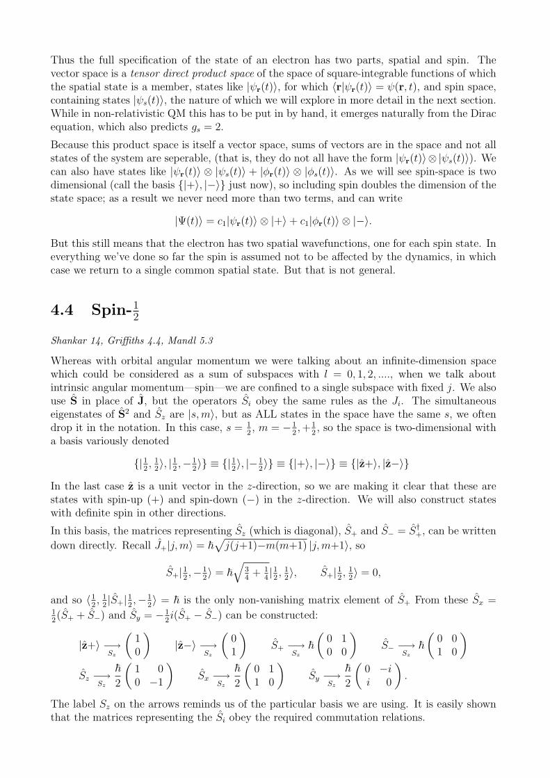
Thus the full specification of the state of an electron has two parts, spatial and spin. Thevector space is a tensor direct product space of the space of square-integrable functions of whichthe spatial state is a member, states like |ψr(t)〉, for which 〈r|ψr(t)〉 = ψ(r, t), and spin space,containing states |ψs(t)〉, the nature of which we will explore in more detail in the next section.While in non-relativistic QM this has to be put in by hand, it emerges naturally from the Diracequation, which also predicts gs = 2.
Because this product space is itself a vector space, sums of vectors are in the space and not allstates of the system are seperable, (that is, they do not all have the form |ψr(t)〉⊗ |ψs(t)〉). Wecan also have states like |ψr(t)〉 ⊗ |ψs(t)〉 + |φr(t)〉 ⊗ |φs(t)〉. As we will see spin-space is twodimensional (call the basis |+〉, |−〉 just now), so including spin doubles the dimension of thestate space; as a result we never need more than two terms, and can write
|Ψ(t)〉 = c1|ψr(t)〉 ⊗ |+〉+ c1|φr(t)〉 ⊗ |−〉.
But this still means that the electron has two spatial wavefunctions, one for each spin state. Ineverything we’ve done so far the spin is assumed not to be affected by the dynamics, in whichcase we return to a single common spatial state. But that is not general.
4.4 Spin-12
Shankar 14, Griffiths 4.4, Mandl 5.3
Whereas with orbital angular momentum we were talking about an infinite-dimension spacewhich could be considered as a sum of subspaces with l = 0, 1, 2, ...., when we talk aboutintrinsic angular momentum—spin—we are confined to a single subspace with fixed j. We alsouse S in place of J, but the operators Si obey the same rules as the Ji. The simultaneouseigenstates of S2 and Sz are |s,m〉, but as ALL states in the space have the same s, we oftendrop it in the notation. In this case, s = 1
2, m = −1
2,+1
2, so the space is two-dimensional with
a basis variously denoted
|12, 1
2〉, |1
2,−1
2〉 ≡ |1
2〉, |−1
2〉 ≡ |+〉, |−〉 ≡ |z+〉, |z−〉
In the last case z is a unit vector in the z-direction, so we are making it clear that these arestates with spin-up (+) and spin-down (−) in the z-direction. We will also construct stateswith definite spin in other directions.
In this basis, the matrices representing Sz (which is diagonal), S+ and S− = S†+, can be written
down directly. Recall J+|j,m〉 = ~√j(j+1)−m(m+1) |j,m+1〉, so
S+|12 ,−12〉 = ~
√34
+ 14|12, 1
2〉, S+|12 ,
12〉 = 0,
and so 〈12, 1
2|S+|12 ,−
12〉 = ~ is the only non-vanishing matrix element of S+ From these Sx =
12(S+ + S−) and Sy = −1
2i(S+ − S−) can be constructed:
|z+〉 −→Sz
(10
)|z−〉 −→
Sz
(01
)S+ −→
Sz
~(
0 10 0
)S− −→
Sz
~(
0 01 0
)Sz −→
Sz
~2
(1 00 −1
)Sx −→
Sz
~2
(0 11 0
)Sy −→
Sz
~2
(0 −ii 0
).
The label Sz on the arrows reminds us of the particular basis we are using. It is easily shownthat the matrices representing the Si obey the required commutation relations.

The matrices
σx =
(0 11 0
)σy =
(0 −ii 0
)σz =
(1 00 −1
)are called the Pauli matrices. They obey σiσj = δijI + i
∑k εijkσk, and a · σb · σ = a · b I +
i(a× b) ·σ. Together with the identity matrix they form a basis (with real coefficients) for allHermitian 2× 2 matrices.
The component of S in an arbitrary direction defined by the unit vector n is S · n, We canparametrise the direction of n by the polar angles θ, φ, so n = sin θ cosφ ex + sin θ sinφ ey +
cos θ ez. Then in the basis of eigenstates of Sz, S · n and its eigenstates are
S·n −→Sz
~2
(cos θ sin θe−iφ
sin θeiφ − cos θ
)|n+〉 −→
Sz
(cos θ
2e−iφ/2
sin θ2eiφ/2
)|n−〉 −→
Sz
(− sin θ
2e−iφ/2
cos θ2eiφ/2
)
Note that (from the matrix representation) (2S · n/~)2 = I for any n. So
exp(i(α/~)S · n
)= cos α
2I + i sin α
22~ S · n.
The lack of higher powers of Si follows from the point about Hermitian operators noted above.
Some calculation in the matrix basis reveals the useful fact that 〈n±|S|n±〉 = ±~2n; that is,
the expectation value of the vector operator S is parallel or antiparallel to n.
Spin precession
The Hamiltonian of a spin-12
electron in a uniform magnetic field is, with gs = 2 and charge−|e|,
H = −µ ·B = (gsµB/~)S ·B −→Sz
µBσ ·B.
Consider the case of a field in the x-direction, so that H −→Sz
µBσxB, and a particle initially
in the state |z+〉. It turns out that we have already done this problem, obtaining, with ω =2µBB/~ being the frequency corresponding to the energy splitting of the eigenstates of H,
|ψ(t)〉 = cos(ωt/2)|z+〉 − isin(ωt/2)|z−〉. 〈ψ(t)|Sz|ψ(t)〉 = (~/2) cosωt.
To this we can now add 〈ψ(t)|Sy|ψ(t)〉 = −(~/2) sinωt, and 〈ψ(t)|Sx|ψ(t)〉 = 0. So the ex-
pectation value of S is a vector of length ~/2 in the yz plane which rotates with frequencyω = 2µBB/~. This is exactly what we would get from Ehrenfest’s theorem.
Alternatively, we can take the magnetic field along z so that the energy eigenstates are |z±〉with energies ±µBB ≡ ±~ω/2. If the initial state is spin-up in an arbitrary direction n, thatis |n+〉, we can decompose this in terms of the energy eigenstates, each with its own energydependence, and obtain
|ψ(t)〉 = cos θ2e−i(ωt+φ)/2|z+〉+ sin θ
2ei(ωt+φ)/2|z−〉 = |n(t)+〉
where n(t) is a vector which, like the original n, is oriented at an angle θ to the z (i.e. B)axis, but which rotates about that axis so that the aximuthal angle changes with time: φ(t) =φ(0) + ωt. The expectation value 〈S〉 precesses likewise, following the same behaviour as aclassical magnetic moment of −gsµB.

Spin and measurement: Stern Gerlach revisited
We now understand, in a way that the orginal experimenters did not, what the Stern-Gerlachexperiment does: for each atom that passes through, it measures S ·n, where the magnetic fieldis along the n direction. Each time, the answer is either up or down, ±~/2. With the initialbeam being unpolarised, the numbers of up and down will be equal.
The apparatus also gives us access to a beam of particles which are all spin-up in a particulardirection; say the z direction. We can then run that beam through a second copy of theapparatus rotated through some angle θ relative to the first. The particles exiting from thiscopy will be either spin-up or down along the new magnetic field axis, and the probability ofgetting each is |〈n ± |z+〉|2, that is cos2 θ
2and sin2 θ
2respectively. If θ = π/2 (new field along
the x axis, assuming a beam in the y-direction), the probabilities are both 50%.
Successive measurements can be schematically represented below; each block being labelled bythe direction of the magnetic field. It should look very familiar.
Higher spins
The Particle Data Group lists spin-1 particles and spin-32
particles; gravitons if they exist arespin-2, and nuclei can have much higher spins (at least 9
2for known ground states of stable
nuclei).
Further more since in many situations total angular momentum commutes with the Hamiltonian(see later) even when orbital angular momentum is involved we are often only concerned witha subspace of fixed j (or l or s). All such sub-spaces are finite dimensional, of dimensionN = 2j + 1, and spanned by the basis |j,m〉 with m = j, j − 1 . . . − j + 1,−j. It is mostusual (though of course not obligatory) to order the states by descending m.
In this subspace, with this basis, the operators Jx, Jy, Jz are represented by three N × N
matrices with matrix elements eg (Jx)m′m = 〈j,m′|Jx|j,m〉. (Because states with differenet jare orthogonal, and because the Ji only change m, not j, 〈j′,m′|Jx|j,m〉 = 0 if j 6= j: that’swhy we can talk about non-overlapping subspaces in the first place.) The matrix representationof Jz of course is diagonal with diagonal elements j, j − 1 . . .− j + 1,−j. As with spin-1
2, it is
easiest to construct J+ first, then J− as its transpose (the elements of the former having beenchosen to be real), then Jx = 1
2(J+ + J−) and Jy = −1
2i(J+ − J−).
As an example we construct the matrix representation of the operators for spin-1. The threebasis states |s,m〉 are |1, 1〉, |1, 0〉 and |1,−1〉. Recall J+|j,m〉 = ~
√j(j+1)−m(m+1) |j,m+1〉,
so S+|1,−1〉 = ~√
2− 0 |1, 0〉, S+|1, 0〉 = ~√
2− 0 |1, 1〉 and S+|1, 1〉 = 0, and the only non-zeromatrix elements of S+ are
〈1, 1|S+|1, 0〉 = 〈1, 0|S+|1,−1〉 =√
2~.
So:

|1, 1〉 −→Sz
100
|1, 0〉 −→Sz
010
|1,−1〉 −→Sz
001
Sz −→
Sz
~
1 0 00 0 00 0 −1
S+ −→Sz
√2~
0 1 00 0 10 0 0
S− −→Sz
√2~
0 0 01 0 00 1 0
Sx −→
Sz
~√2
0 1 01 0 10 1 0
Sy −→Sz
~√2
0 −i 0i 0 −i0 i 0
Of course this is equally applicable to any system with j = 1, including the l = 1 sphericalharmonics.
Once all possible values of j and m are allowed, any angular momentum operator is representedin the |j,m〉 = |0, 0〉, |1
2, 1
2〉, |1
2,−1
2〉, |1, 1〉, |1, 0〉, |1,−1〉 . . . basis by a block-diagonal matrix
The first block is a single element, zero in fact, since all components of J in the one-dimensionalspace of states of j = 0 are zero. The next block is the appropriate 2×2 spin-1
2matrix, the next
a 3× 3 spin-1 matrix, and so on. This block-diagonal structure reflects the fact that the vectorspace can be written as a direct sum of spaces with j = 0, j = 1
2, j = 1....: V = V1⊕V2⊕V3⊕. . .
(where the superscripts of course are 2j + 1).
In fact, any given physical system can only have integer or half-integer angular momentum.So the picture would be similar, but with only odd- or even-dimensioned blocks. For orbitalangular momentum, for instance, the blocks would be 1× 1, 3× 3, 5× 5 . . ..

4.5 Addition of angular momentum
Shankar pp 403-415, Griffiths 4.4, Mandl 4.4
Up till now, we have in general spoken rather loosely as if an electron has either orbital orspin angular momentum—or more precisely, we’ve considered cases where only one affects thedynamics, so we can ignore the other. But many cases are not like that. If a hydrogen atomis placed in a magnetic field, its electron can have both orbital and spin angular momentum,and both will affect how the energy levels shift, and hence how the spectral lines split. Or thedeuteron (heavy hydrogen nucleus) consists of both a proton and a neutron, and both havespin; heavier atoms and nuclei have many components all with spin and angular momentum.Only the total angular momentum of the whole system is guaranteed by rotational symmetryto be conserved in the absence of external fields. So we need to address the question of theaddition of angular momentum.
Because the notation is clearest, we will start with the spin and orbital angular momentum ofa particle. We consider the case where l as well as s is fixed: electrons in a p-wave orbital,for instance. These two types of angular momentum are independent and live in differentvector spaces, so this is an example of a tensor direct product space, spanned by the basis|l,ml〉 ⊗ |s,ms〉 and hence (2l + 1)× (2s+ 1) dimensional.
Now angular momentum is a vector, and we expect the total angular momentum to be thevector sum of the orbital and spin angular momenta. We can form a new vector operator inthe product space
J = L⊗ I + I ⊗ S J2 = L2 ⊗ I + I ⊗ S2 + 2L⊗ S
where the last term represents a scalar product as well as a tensor product and would moreclearly be written 2(Lx ⊗ Sx + Ly ⊗ Sy + Lz ⊗ Sz).In practice, the tensor product notation for operators proves cumbersome, and we always justwrite
J = L + S J2 = L2 + S2 + 2L · S
We know that the Li and Si act on different parts of the state, and we don’t need to stress thatwhen we act with Si alone we are not changing the orbital state, etc. An alternative form, inwhich the tensor product notation is again suppressed, is
J2 = L2 + S2 + L+S− + L−S+ + 2LzSz.
Now in calling the sum of angular momenta J, which we previously used for a generic angularmomentum, we are assuming that the Ji do indeed obey the defining commutation rules forangular momentum, and this can easily be demonstrated. For instance
[Jx, Jy] = [Lx + Sx, Ly + Sy] = [Lx, Ly] + [Sx, Sy] = i~Lz + i~Sz = i~Jz,
where we have used the fact that [Li, Sj] = 0, since they act in different spaces. Hence weexpect that an alternative basis in the product space will be |j,mj〉, with allowed values ofj not yet determined. The question we want to answer, then, in the connection between the|l,ml〉 ⊗ |s,ms〉 and |j,mj〉 bases. Both, we note, must have dimension (2l+ 1)× (2s+ 1).
We note some other points about the commutator: Lz, Sz and Jz all commute; Jz commuteswith J2 (of course) and with L2 and with S2 (because both Lz and Sz do), but Lz and Sz do notcommute with J2. Thus we can, as implied when we wrote down the two bases, always specify

l and s, but then either ml and ms (with mj = ml+ms) or j and mj. (We will sometimes write|l, s; j,mj〉 instead of just |j,mj〉, if we need a reminder of l and s in the problem.) What thisboils down to is that the state of a given j and mj will be linear superpositions of the states ofgiven ms and ml that add up to that mj. If there is more than one such state, there must bemore than one allowed value of j for that mj.
Let’s introduce a useful piece of jargon: the state of maximal m in a multiplet, |j, j〉, is calledthe stretched state.
We start with the state of maximal ml and ms |l, l〉 ⊗ |s, s〉, which has mj = l + s. This isclearly the maximal value of mj, and hence of j: jmax = l + s, and since the state is unique, it
must be an eigenstate of J2 3. If we act on this with J− = L− + S−, we get a new state withtwo terms in it; recalling the general rule J−|j,m〉 = ~
√j(j + 1)−m(m− 1)|j,m−1〉 where j
can stand for j or l or s, we have (using as a shorthand for jmax = l + s)
|, 〉 = |l, l〉 ⊗ |s, s〉 ⇒ J−|, 〉 = (L−|l, l〉)⊗ |s, s〉+ |l, l〉 ⊗ (S−|s, s〉)⇒√
2 |, −1〉 =√
2l |l, l−1〉 ⊗ |s, s〉+√
2s |l, l〉 ⊗ |s, s−1〉
From this state we can continue operating with J−; at the next step there will be three terms onthe R.H.S. with ml,ms equal to l−2, s, l−1, s−1 and l, s−2, then four, but eventuallywe will reach states which are annihilated by L− or S− and the number of terms will start toshrink again, till we finally reach |,−〉 = |l,−l〉 ⊗ |s,−s〉 after 2 steps (2 + 1 states in all).Whichever is the smaller of l or s will govern the maximum number of ml,ms that can equalany mj; for example if s is smaller, the maximum number is 2s+ 1.
Now the state we found with mj = l+s−1 is not unique, there must be another orthogonalcombination of the two states with ml,ms equal to l−1, s and l, s−1. This cannot bepart of a multiplet with j = because we’ve “used up” the only state with mj = . So it mustbe the highest mj state (the stretched state) of a multiplet with j = − 1 (ie l + s− 1):
|− 1, − 1〉 = −√
sl+s|l, l−1〉 ⊗ |s, s〉+
√ll+s|l, l〉 ⊗ |s, s−1〉
Successive operations with J− will generate the rest of the multiplet (2−1 in all); all the stateswill be orthogonal to the states of the same mj but higher j already found.
However there will be a third linear combination of the states with ml,ms equal to l−2, s,l−1, s−1 and l, s−2, which cannot have j = or −1. So it must be the stretched state ofa multiplet with j = −2, (2− 3 states in all).
And so it continues, generating multiplets with successively smaller values of j. However theprocess will come to an end. As we saw, the maximum number of terms in any sum is whicheveris smaller of 2l+ 1 or 2s+ 1, so this is also the maximum number of mutually orthogonal statesof the same mj, and hence the number of different values of j. So j can be between l + s andthe larger of l+ s− 2s and l+ s− 2l; that is, l+ s ≥ j ≥ |l− s|. The size of the |j,mj〉 basis
is then∑l+s
j=|l−s| 2j + 1, which is equal to (2l + 1)(2s+ 1).
The table below illustrates the process for l = 2, s = 1; we go down a column by applying J−,and start a new column by constructing a state orthogonal to those in the previous columns.The three columns correspond to j = 3, j = 2 and j = 1, and there are 7 + 5 + 3 = 5× 3 statesin total.
3This can also be seen directly by acting with J2 = J−J+ + J2z + ~Jz, since |l, l〉 ⊗ |s, s〉 is an eigenstate of
Jz with eigenvalue ~(l + s), and is annihilated by both L+ and S+, and hence by J+.

|3, 3〉 = |2, 2〉⊗|1, 1〉|3, 2〉 =
q23 |2, 1〉⊗|1, 1〉+
q13 |2, 2〉⊗|1, 0〉 |2, 2〉 = −
q13 |2, 1〉⊗|1, 1〉+
q23 |2, 2〉⊗|1, 0〉
|3, 1〉 =q
25 |2, 0〉⊗|1, 1〉+
q815 |2, 1〉⊗|1, 0〉 |2, 1〉 = −
q12 |2, 0〉⊗|1, 1〉+
q16 |2, 1〉⊗|1, 0〉 |1, 1〉 =
q110 |2, 0〉⊗|1, 1〉−
q310 |2, 1〉⊗|1, 0〉
+q
115 |2, 2〉⊗|1,−1〉 +
q13 |2, 2〉⊗|1,−1〉 +
q35 |2, 2〉⊗|1,−1〉
|3, 0〉 =q
15 |2,−1〉⊗|1, 1〉+
q35 |2, 0〉⊗|1, 0〉 |2, 0〉 = −
q12 |2,−1〉⊗|1, 1〉+0|2, 0〉⊗|1, 0〉 |1, 0〉 =
q310 |2,−1〉⊗|1, 1〉−
q25 |2, 0〉⊗|1, 0〉
+q
15 |2, 1〉⊗|1,−1〉 +
q12 |2, 1〉⊗|1,−1〉 +
q310 |2, 1〉⊗|1,−1〉
|3,−1〉 =q
115 |2,−2〉⊗|1, 1〉+
q815 |2,−1〉⊗|1, 0〉 |2,−1〉 = −
q13 |2,−2〉⊗|1, 1〉−
q16 |2,−1〉⊗|1, 0〉 |1,−1〉 =
q35 |2,−2〉⊗|1, 1〉−
q310 |2,−1〉⊗|1, 0〉
+q
25 |2, 0〉⊗|1,−1〉 +
q12 |2, 0〉⊗|1,−1〉 +
q110 |2, 0〉⊗|1,−1〉
|3,−2〉 =q
13 |2,−2〉⊗|1, 0〉+
q23 |2,−1〉⊗|1,−1〉 |2,−2〉 = −
q23 |2,−2〉⊗|1, 0〉+
q13 |2,−1〉⊗|1,−1〉
|3,−3〉 = |2,−2〉⊗|1,−1〉
The coefficients in the table are called Clebsch-Gordan coefficients. They are the inner prod-ucts (〈l,ml| ⊗ 〈s,ms|)|j,mj〉 but that is too cumbersome a notation; with a minimum modifi-cation Shankar uses 〈l,ml; s,ms|j,mj〉; Mandl uses C(l,ml, s,ms; j,mj), but 〈l, s,ml,ms|j,mj〉and other minor modifications, including dropping the commas, are common. They are alltotally clear when symbols are being used, but easily confused when numerical values are sub-stituted! We use the “Condon-Shortley” phase convention, which is the most common; in thisconvention Clebsch-Gordan coefficients are real, which is why we won’t write 〈l,ml; s,ms|j,mj〉∗in the second equation of Eq. (4.5) below. General formulae for the coefficients are not used(the case of s = 1
2is an exception, see below), instead one consults tables or uses the Math-
ematica function ClebschGordan[l,ml, s,ms, j,mj]. There is also an on-line calculatorat Wolfram Alpha.
Here you will find the PDG tables of Clebsch-Gordan coefficients and here instructions on theiruse.
All of this has been written for the addition of orbital and spin angular momenta. But we didnot actually assume at any point that l was integer. So in fact the same formulae apply forthe addition of any two angular momenta of any origin: a very common example is two spin-1
2
particles. The more general form for adding two angular momenta j1 and j2, with J and Mbeing the quantum numbers corresponding to the total angular momentum of the system, is
|J,M〉 =∑m1,m2
〈j1,m1; j2,m2|J,M〉 |j1,m1〉 ⊗ |j2,m2〉,
|j1,m1〉 ⊗ |j2,m2〉 =∑J,M
〈j1,m1; j2,m2|J,M〉 |J,M〉. (4.5)
For the common case of s = 12, j = l ± 1
2, we have
|l±12,mj〉 =
√l∓mj+
12
2l+1|l,mj+
12〉 ⊗ |1
2,−1
2〉 ±
√l±mj+
12
2l+1|l,mj−1
2〉 ⊗ |1
2, 1
2〉.
To summarise, the states of a system with two contributions to the angular momentum, j1and j2, written in a basis in which the total angular momentum J and z-component M arespecified; the values of J range from |j1−j2| to j1+j2 in unit steps. In this basis the total angularmomentum operators Ji and J2 are cast in block-diagonal form, one (2J+1)-square block foreach value of J . The vector space, which we started by writing as a product, V2j1+1 ⊗ V2j2+1,can instead be written as a direct sum: V2(j1+j2)+1 ⊕ . . . ⊕ V2|j1−j2|+1. In particular for someorbital angular momentum l and s = 1
2, V2l+1 ⊗ V2 = V2l+2 ⊕ V2l. The overall dimension of
the space is of course unchanged.
Example: Two spin-12 particles
Here we will call the operators S(1), S(2) and S = S(1) + S(2) for the individual and total spinoperators, and S and M for the total spin quantum numbers. (The use of capitals is standard

in a many-particle system.) Because both systems are spin-12, we will omit the label from our
states, which we will write in the m1,m2 basis as
|1〉 = |+〉 ⊗ |+〉, |2〉 = |+〉 ⊗ |−〉, |3〉 = |−〉 ⊗ |+〉, |4〉 = |−〉 ⊗ |−〉.
(The 1 . . . 4 are just labels here.) In this basis
S+ −→ ~
0 1 1 00 0 0 10 0 0 10 0 0 0
Sz −→ ~
1 0 0 00 0 0 00 0 0 00 0 0 −1
S2 −→ ~2
2 0 0 00 1 1 00 1 1 00 0 0 2
where we use explicit calculation for the matrix elements, eg
〈1|(S(1)
+ + S(2)
+ )|2〉 = 〈+|S(1)
+ |+〉〈+|I (2)|−〉+ 〈+|I (1)|+〉〈+|S(2)
+ |−〉 = 0 + ~,
then S− = (S+)† and S2 = S+S− + S2z − ~Sz.
It is clear that |1〉 and |4〉 are eigenstates of S2 with eigenvalue 2~2 and hence S = 1. They arealso eigenstates of Sz with eigenvalues ±~. In the |2〉, |3〉 subspace, which has M = 0, S2 is
represented by the matrix ~2
(1 11 1
)which has eigenvalues 2~2 and 0 corresponding to states√
12(|2〉 ± |3〉). We label these four simultaneous eigenstates of S2 and Sz as |S,M〉, and take
the ordering for the new basis as |0, 0〉, |1, 1〉, |1, 0〉, |1,−1〉. Then the matrix of eigenvectors,U, is
U = ~
0 1 0 0
1/√
2 0 1/√
2 0
−1/√
2 0 1/√
2 00 0 0 1
and the transformed matrices U†SiU are
Sx −→~√2
0 0 0 00 0 1 00 1 0 10 0 1 0
Sy −→~√2
0 0 0 00 0 −i 00 i 0 −i0 0 i 0
Sz −→ ~
0 0 0 00 1 0 00 0 0 00 0 0 −1
where the 1× 1 plus 3× 3 block-diagonal structure has been emphasised and the 3× 3 blocksare just the spin-1 matrices we found previously.
Angular Momentum of Atoms and Nuclei
Both atoms and nuclei consist of many spin-12
fermions, each of which has both spin and orbitalangular momentum. In the independent-particle model we think of each fermion occupying awell-defined single-particle orbital which is an eigenstate of a central potential and hence haswell defined orbital angular momentum l. The notation s, p, d, f , g. . . is used for orbitals ofl = 0, 1, 2, 3, 4 . . .. For each fermion there is also a total angualar momentum j, and the spin-orbit splitting (of which more later) splits states of different j. All the angular momenta of allthe fermions can be added in a variety of ways, and the following quantum numbers are defined:L for the sum of all the orbital angular momenta (that is, the eigenvalues of L2
tot are ~2L(L+1));S for the sum of all the spin angular momenta, and J for the total angular momentum of the

atom or nucleus from all sources. The use of capitals for the quantum numbers shouldn’t beconfused with the operators themselves.
In reality the independent-particle model is only an approximation, and only the total angularmomentum J is a conserved quantum number (only J2
tot commutes with the Hamiltonian ofthe whole system). For light atoms, it is a good starting point to treat L and S as if they wereconserved too, and the notation 2S+1LJ is used, with L being denoted by S, P , D, F , G. . . .This is termed LS coupling. So 3S1 has L = 0, S = J = 1. For heavy atoms and nuclei, it is abetter approximation to sum the individual total angular momenta j. (j-j coupling.)
Somewhat confusingly, J is often called the spin of the atom or nucleus, even though its originis both spin and angular momentum. This composite origin shows up in a magnetic couplingg which is neither 1 (pure orbital) or 2 (pure spin). For light atoms g can be calculated fromL, S and J (the Lande g-factor). For nuclei things are further complicated by the fact thatprotons and neutrons are not elementary particles, and their “spin” is likewise of compositeorigin, something which shows up through their g values of gp = 5.59 and gn = −3.83 ratherthan 2 and 0 respectively. Using these the equivalent of the Lande g-factor can be calculatedfor individual nucleon orbitals, and hence for those odd-even nuclei for which the single-particlemodel works (that is, assuming that only the last unpaired nucleon contributes to the totalangular momentum). Beyond that it gets complicated.
4.6 Vector Operators
Shankar 15.3
This section is not examinable. The take-home message is that vector operators such as xand p can change the angular momentum of the state they act on in the same way as couplingin another source of angular momentum with l = 1. If the components of the vector operatorare written in a spherical basis analogously to J±, the dependence of the matrix elements on them quantum numbers is given by Clebsch Gordan coefficients, with the non-trivial dependenceresiding only in a single “reduced matrix element” for each pair j and j′ of the angular momentaof the initial and final states. This is the Wigner-Eckart theorem of Eq. (4.6).
We have now met a number of vector operators: x = (x, y, z), p = (px, py, pz), and of course
L, S and J. We have seen, either in lectures or examples, that they all satisfy the followingrelation: if V stands for the vector operator
[Ji, Vj] =∑k
i~ εijk Vk
for example, [Jx, y] = i~z. (We could have substituted Lx for Jx here as spin and space operatorscommute.)
We can take this to be the definition of a vector operator: a triplet of operators makes up avector operator if it satisfies these commutation relations.
Just as it was useful to define J+ and J−, so it is useful to define
V+1 = −√
12(V1 + iV2) V−1 =
√12(V1 − iV2) V0 = V3
where the subscripts are no longer Cartesian coordinates (1 ≡ x etc) but analogous to the mof the spherical harmonics—and indeed
∓√
12(x± iy) =
√4π3rY ±1
1 (θ, φ) z =√
4π3rY 0
1 (θ, φ).

Note a slight change of normalisation and sign: J±1 = ∓√
12J±. In terms of these spherical
components Vm,
[J0, Vm] = m~Vm [J±, Vm] = ~√
(1∓m)(2±m)Vm±1
If we compare these to the effects on states
J3|j,m〉 = ~m|j,m〉 J±|j,m〉 = ~√
(j ∓m)(j ±m+ 1)|j,m± 1〉
we see a close parallel, so long as we take j = 1 for the vector operators.4
Consider the following two calculations. First, we consider matrix elements of the commutatorof the components of a tensor operator Vm with J±, in which l = 1, and p and q are magneticquantum numbers like m; in the second line we note that 〈j,m|J± is the bra associated withJ∓|j,m〉
〈j′, p|[J±, Vm]|j, q〉 = ~√
(l ∓m)(l ±m+ 1)〈j′, p|Vm±1|j, q〉and 〈j′, p|J±Vm − VmJ±|j, q〉 = ~
√(j′ ± p)(j′ ∓ p+ 1)〈j′, p∓ 1|Vm|j, q〉− ~√
(j ∓ q)(j ± q + 1)〈j′, p|Vm|j, q ± 1〉⇒√
(l ∓m)(l ±m+ 1)〈j′, p|Vm±1|j, q〉 =√
(j′ ± p)(j′ ∓ p+ 1)〈j′, p∓ 1|Vm|j, q〉−√
(j ∓ q)(j ± q + 1)〈j′, p|Vm|j, q ± 1〉
Secondly we take matrix elements of J± = J (1)
± + J (2)
± , giving us a relation between the Clebsch-Gordan coefficients for l and j coupling up to j′
〈j′, p|J±(|l,m〉 ⊗ |j, q〉
)= ~√
(j′ ± p)(j′ ∓ p+ 1)〈j′, p∓ 1|l,m; j, q〉
and 〈j′, p|J (1)
± + J (2)
±
(|l,m〉 ⊗ |j, q〉
)= ~√
(l ∓m)(l ±m+ 1)〈j′, p|l,m± 1; j, q〉
+ ~√
(j ∓ q)(j ± q + 1)〈j′, p|l,m; j, q ± 1〉⇒√
(l ∓m)(l ±m+ 1)〈j′, p|l,m± 1; j, q〉 =√
(j′ ± p)(j′ ∓ p+ 1)〈j′, p∓ 1|l,m; j, q〉−√
(j ∓ q)(j ± q + 1)〈j′, p|l,m; j, q ± 1〉
Comparing the two, we see that the coefficients are identical, but in the first they multiplymatrix elements of V whereas in the second, they multiply Clebsch-Gordan coefficients. Thiscan only be true if the matrix elements are proportional to the Clebsch-Gordan coefficients,with a constant of proportionality which must be independent of magnetic quantum numbers,and which we will write as 〈j′||V||j〉, the reduced matrix element:
〈j′, p|Vm|j, q〉 = 〈j′||V||j〉〈j′, p|l,m; j, q〉|l=1
This is a specific instance of the Wigner-Eckart theorem. It says that acting on a statewith a vector operator is like coupling in one unit of angular momentum; only states with|j′ − 1| ≤ j ≤ j′ + 1 and with p = m + q will have non-vanishing matrix elements. It alsomeans that if one calculates one matrix element, which ever is the simplest (so long as it isnon-vanishing), then the others can be written down directly.
Since J is a vector operator, it follows that matrix elements of Jq can also be written in terms
of a reduced matrix element 〈j′||J||j〉, but of course this vanishes unless j′ = j.
4Note that in this section, we use the algebraically equivalent (j ∓m)(j ±m + 1) for j(j + 1)−m(m± 1) inthe normalisation of J±|j,m〉.
Writing |j1, j2; J,M〉 =∑
m1m2〈J,M |j1,m1; j2,m2〉|j1,m1〉⊗ |j2,m2〉, and using orthonormality
of the states |J,M〉, allows us to show that∑m1m2
〈J,M |j1,m1; j2,m2〉〈J ′,M ′|j1,m1; j2,m2〉 = δJJ ′δMM ′ (4.6)
Noting too that a scalar product of vector operators P·Q can be written in spherical componentsas∑
q(−1)qP−qQq, we can show that
〈j,m|P · J|j,m〉 =∑q,j′,m′
(−1)q〈j,m|P−q|j′,m′〉〈j′,m′|Jq|j,m〉
=∑q,m′
〈j′,m′|Pq|j,m〉〈j′,m′|Jq|j,m〉 = 〈j||P||j〉〈j||J||j〉;
(we insert a complete set of states at the first step, then use the Wigner-Eckart theorem andEq. (4.6)).
Replacing P with J gives us 〈j||J||j〉 =√j(j + 1). Hence we have the extremely useful relation
〈j,m|P|j,m〉 = 〈j,m|J|j,m〉〈j,m|P · J|j,m〉j(j + 1)
. (4.7)
which we will use in calculating the Lande g factor in the next section.
Finally, we might guess from the way that we used a general symbol l instead of 1, that thereare operators which couple in 2 or more units of angular momentum. Simple examples areobtained by writing rlY m
l in terms of x, y and z, then setting x→ x etc; so (x± iy)2, (x± iy)z,and 2z2 − x2 − y2) are the m = ±2, m = ±1 and m = 0 components of an operator withl = 2 (a rank-two tensor operator, in the jargon). There are six components of xixj, but(z2 + x2 + y2) is a scalar (l = 0). This is an example of the tensor product of two l = 1 operatorsgiving l = 2 and l = 0 operators.

Time-independent perturbation theory
5.1 Approximate methods in Quantum Mechanics
It is often (almost always!) the case that we cannot solve real problems analytically. Only avery few potentials have analytic solutions, by which I mean one can write down the energylevels and wave functions in closed form, as for the harmonic oscillator and Coulomb potential.In fact those are really the only useful ones (along with square wells)... In the last century,a number of approximate methods have been developed to obtain information about systemswhich can’t be solved exactly.
These days, this might not seem very relevant. Computers can solve differential equations veryefficiently. But:
• It is always useful to have a check on numerical methods
• Even supercomputers can’t solve the equations for many interacting particle exactly in areasonable time (where “many” may be as low as four, depending on the complexity ofthe interaction) — ask a nuclear physicist or quantum chemist.
• Quantum field theories are systems with infinitely many degrees of freedom. All ap-proaches to QFT must be approximate.
• If the system we are interested in is close to a soluble one, we might obtain more insightfrom approximate methods than from numerical ones. This is the realm of perturbationtheory. The most accurate prediction ever made, for the anomalous magnetic moment ofthe electron, which is good to one part in 1012, is a 4th order perturbative calculation.
Examples of approximate methods that we will not cover in this course are:
• The WKB approximation, applicable when the potential varies slowly on the scale ofthe wavelength of a particle moving in that potential. Among other uses, it gives anapproximation expression for the probability of tunnelling through a barrier. Recall thatfor a square barrier of height V and width L this is proportional to exp(−2kL), where
k =√
2m(V − E). For a slowly varying potential, this is replaced by exp(−2∫ L
0k(x)dx),
where k(x) =√
2m(V (x)− E). You will meet this in the context of alpha decay; thedetails are given here.
• The variational method, which sets an upper bound on the ground-state energy E0 ofa bound system, by noting that for any appropriate normalised trial state |Ψ〉, E0 ≤〈Ψ|H|Ψ〉, something that can easily be seen by expressing |Ψ〉as a sum over the trueeigenstates of H.
By far the most widely used approximate method, though, is perturbation theory, applicablewhere the problem to be solved is “close to” a soluble one.
55

5.2 Non-degenerate perturbation theory
Shankar 17.1, Mandl 7.1, Griffiths 6.1
Perturbation theory is applicable when the Hamiltonian H can be split into two parts, with thefirst part being exactly solvable and the second part being small in comparison. The first partis always written H (0), and we will denote its eigenstates by |n(0)〉 and energies by E(0)
n (withwave functions φ(0)
n ). These we know. The eigenstates and energies of the full Hamiltonian aredenoted |n〉 and En, and the aim is to find successively better approximations to these. Thezeroth-order approximation is simply |n〉 = |n(0)〉 and En = E(0)
n , which is just another wayof saying that the perturbation is small and at a crude enough level of approximation we canignore it entirely.
Nomenclature for the perturbing Hamiltonian H − H (0) varies. δV , H (1) and λH (1) are allcommon. It usually is a perturbing potential but we won’t assume so here, so we won’t use thefirst. The second and third differ in that the third has explicitly identified a small, dimensionlessparameter (eg α in EM), so that the residual H (1) isn’t itself small. With the last choice, ourexpressions for the eigenstates and energies of the full Hamiltonian will be explicitly powerseries in λ, so En = E(0)
n + λE(1)n + λ2E(2)
n + . . . etc. With the second choice the small factor ishidden in H (1), and is implicit in the expansion which then reads En = E(0)
n +E(1)n +E(2)
n + . . .. Inthis case one has to remember that anything with a superscript (1) is first order in this implicitsmall factor, or more generally the superscript (m) denotes something which is mth order. Forthe derivation of the equations we will retain an explicit λ, but thereafter we will set it equalto one to revert to the other formulation. We will take λ to be real so that H1 is Hermitian.
We start with the master equation
(H (0) + λH (1))|n〉 = En|n〉.
Then we substitute in En = E(0)n + λE(1)
n + λ2E(2)n + . . . and |n〉 = |n(0)〉+ λ|n(1)〉+ λ2|n(2)〉+ . . .
and expand. Then since λ is a free parameter, we have to match terms on each side with thesame powers of λ, to get
H (0)|n(0)〉 = E(0)
n |n(0)〉H (0)|n(1)〉+ H (1)|n(0)〉 = E(0)
n |n(1)〉+ E(1)
n |n(0)〉H (0)|n(2)〉+ H (1)|n(1)〉 = E(0)
n |n(2)〉+ E(1)
n |n(1)〉+ E(2)
n |n(0)〉
We have to solve these sequentially. The first we assume we have already done. The secondwill yield E(1)
n and |n(1)〉. Once we know these, we can use the third equation to yield E(2)n and
|n(2)〉, and so on. The expressions for the changes in the states, |n(1)〉 etc, will make use of thefact that the unperturbed states |n(0)〉 from a basis, so we can write
|n(1)〉 =∑m
cm|m(0)〉 =∑m
〈m(0)|n(1)〉 |m(0)〉.
In each case, to solve for the energy we take the inner product with 〈n(0)| (i.e. the same state)whereas for the wave function, we use 〈m(0)| (another state). We use, of course, 〈m(0)|H (0) =E(0)m 〈m(0)| and 〈m(0)|n(0)〉 = δmn.
At first order we get
E(1)
n = 〈n(0)|H (1)|n(0)〉 (5.1)
〈m(0)|n(1)〉 =〈m(0)|H (1)|n(0)〉E(0)n − E(0)
m
∀m 6= n.

The second equation tells us the overlap of |n(1)〉 with all the other |m(0)〉, but not with |n(0)〉.This is obviously not constrained by the eigenvalue equation, because we can add any amountof |n(0)〉 and the equations will still be satisfied. However we need the state to continue to benormalised, and when we expand 〈n|n〉 = 1 in powers of λ we find that 〈n(0)|n(1)〉 is requiredto be imaginary. This is just like a phase rotation of the original state and we can ignore it.(Recall that an infinitesimal change in a unit vector has to be at right angles to the original.)Hence
|n(1)〉 =∑m6=n
〈m(0)|H (1)|n(0)〉E(0)n − E(0)
m
|m(0)〉. (5.2)
If the spectrum of H (0) is degenerate, there may be a problem with this expression because thedenominator can be infinite. In fact nothing that we have done so far is directly valid in thatcase, and we have to use “degenerate perturbation theory” instead. For now we assume that forany two states |m(0)〉 and |n(0)〉, either E(0)
n − E(0)m 6= 0 (non degenerate) or 〈m(0)|H (1)|n(0)〉 = 0
(the states are not mixed by the perturbation.)
Then at second order
E(2)
n = 〈n(0)|H (1)|n(1)〉 =∑m 6=n
∣∣∣〈m(0)|H (1)|n(0)〉∣∣∣2
E(0)n − E(0)
m
. (5.3)
The expression for the second-order shift in the wave function |n(2)〉 can also be found but itis tedious. The main reason we wanted |n(1)〉 was to find E(2)
n anyway, and we’re not planningto find E(3)
n ! Note that though the expression for E(1)n is generally applicable, those for |n(1)〉
and E(2)n would need some modification if the Hamiltonian had continuum eigenstates as well
as bound states (eg hydrogen atom). Provided the state |n〉 is bound, that is just a matter ofintegrating rather than summing. This restriction to bound states is why Mandl calls chapter 7“bound-state perturbation theory”. The perturbation of continuum states (eg scattering states)is usually dealt with separately.
Note that the equations above hold whether we have identified an explicit small parameter λor not. So from now on we will set λ to one, assume that H (1) has an implicit small parameterwithin it, and write En = E(0)
n +E(1)n +E(2)
n + . . .; the expressions above for E(1,2) and |n(1)〉 arestill valid.
5.2.1 Connection to variational approach
It can be shown that 〈ψ|H|ψ〉 ≥ E0 for all normalised states |ψ〉 (with equalitiy implying|ψ〉 = |0〉). This is the basis of the variational approach to finding the ground state energy,where we vary the a trial state |ψ〉 to minimise our upper bound on E0.
For the ground state (which is always non-degenerate) E(0)
0 + E(1)
0 is an upper bound on theexact energy E0, since it is obtained by using the unperturbed ground state as a trial wavefunction for the full Hamiltonian. It follows that the sum of all higher corrections E(2)
0 + . . .must be negative. We can see indeed that E(2)
0 will always be negative, since for every term inthe sum the numerator is positive and the denominator negative.

5.2.2 Simple examples of perturbation theory: 1
Probably the simplest example we can think of is an infinite square well with a low step halfway across, so that
V (x) =
0 for 0 < x < a/2,
V0 for a/2 < x < a
∞ elsewhere
We treat this as a perturbation on the flat-bottomed well, so H (1) = V0 for a/2 < x < a andzero elsewhere.
The ground-state unperturbed wave function is ψ(0)
0 =√
2a
sin πxa
, with unperturbed energy
E(0)
0 = π2~2/(2ma2). A “low” step will mean V0 E(0)
0 . Then we have
E(1)
0 = 〈ψ(0)
0 |H (1)|ψ(0)
0 〉 =2
a
∫ a
a/2
V0 sin2 πx
adx =
V0
2
This problem can be solved semi-analytically; in both regions the solutions are sinusoids, butwith wavenumbers k =
√2mE/~ and k′ =
√2m(E − V0)/~ respectively; satisfying the bound-
ary conditions and matching the wave functions and derivatives at x = a/2 gives the conditionk cot(ka/2) = k′ cot(k′a/2) which can be solved numerically for E. Below the exact solu-tion (green, dotted) and E(0)
0 + E(1)
0 (blue) are plotted; we can see that they start to divergewhen V0 is about 5, which is higher than we might have expected (everything is in units of~2/(2ma2) ≈ 0.1E0).
2 4 6 8 10 12 14V
11
12
13
14
15
16
17
E
We can also plot the exact wave functions for different step size, and see that for V0 = 10 (themiddle picture, well beyond the validity of first-order perturbation theory) it is significantlydifferent from a simple sinusoid.
0.0 0.2 0.4 0.6 0.8 1.0
5
10
15
20
25
0.0 0.2 0.4 0.6 0.8 1.0
5
10
15
20
25
0.0 0.2 0.4 0.6 0.8 1.0
5
10
15
20
25
5.2.3 Simple examples of perturbation theory: 2
Another example is the harmonic oscillator, H = p2
2m+ 1
2mω2x2, with a perturbing potential
H (1) = λx2. The states of the unperturbed oscillator are denoted |n(0)〉 with energies E(0)
0 =

(n+ 12)~ω.
Recalling that in terms of creation and annihilation operators (see section A.1),x = (x0/
√2)(a+ a†), with [a, a†] = 1, and x0 =
√~/(mω), and so
E(1)
n = 〈n(0)|H (1)|n(0)〉 =x2
0λ
2〈n(0)|(a†)2 + a2 + 2a†a+ 1|n(0)〉 =
λ
mω2~ω(n+ 1
2).
The first-order change in the wave function is also easy to compute, as 〈m(0)|H (1)|n(0)〉 = 0unless m = n± 2. Thus
|n(1)〉 =∑m6=n
〈m(0)|H (1)|n(0)〉E(0)n − E(0)
m
|m(0)〉
=~λ
2mω
(√(n+ 1)(n+ 2)
−2~ω|(n+ 2)(0)〉+
√n(n− 1)
2~ω|(n− 2)(0)〉
).
We can now also calculate the second order shift in the energy:
E(2)
n = 〈n(0)|H (1)|n(1)〉 =∑m6=n
∣∣∣〈m(0)|H (1)|n(0)〉∣∣∣2
E(0)n − E(0)
m
=
(~λ
2mω
)2((n+ 1)(n+ 2)
−2~ω+n(n− 1)
2~ω
)= −1
2
(λ
mω2
)2 ~ω(n+ 12)
We can see a pattern emerging, and of course this is actually a soluble problem, as all that theperturbation has done is change the frequency. Defining ω′ = ω
√1 + 2λ/(mω2), we see that
the exact solution is
En = (n+ 12)~ω′ = (n+ 1
2)~ω
(1 + λ
mω2 − 12
(λ
mω2
)2+ . . .
)in agreement with the perturbative calculation.
5.3 Degenerate perturbation theory
Shankar 17.3, Mandl 7.3, Griffiths 6.6
None of the formalism that we have developed so far works if H (0) has degenerate eigenstates.To be precise, it is still fine for the non-degenerate states, but it fails to work in a subspace ofdegenerate states if H (1) not also diagonal in this subspace. The reason is simple: we assumedfrom the start that the shifts in the states due to the perturbation would be small. But
suppose |1(0)〉 and |2(0)〉 are degenerate eigenstates of H (0); then so are√
12
(|1(0)〉± |2(0)〉
). Now
the eigenstate of the full Hamiltonian |1〉 and |2〉 are not degenerate—but which of the possiblechoices for the eigenstate of H (0) are they close to? If for example it is the latter (as is oftenthe case) then even a tiny perturbation H (1) will induce a big change in the eigenstates.
The solution is clear: we need to work with a combination of the unperturbed degenerate statesin which H (1) is diagonal. Sometimes the right choice is obvious from the outset. To use aphysical example, if H (0) commutes with both L and S, we have a choice of quantum numbersto classify the state, our basis can be |l,ml; s,ms〉 or |l, s; j,mj〉. If H (1) fails to commute

with L or S (while still commuting with L2 and S2), then we avoid all problems by simplychoosing the second basis from the start.5
In the absence of physical guidance, we need to write down the matrix which is the representa-tion of H (1) in the degenerate subspace of the originally-chosen basis, and diagonalise it. Theeigenstates are still eigenstates of H (0) and are linear combinations of the old basis states. Wethen then proceed as in the non-degenerate case having replaced (say) |1(0)〉 and |2(0)〉 with thenew linear combinations which we can call |1′(0)〉 and |2′(0)〉. The expressions for the energy andstate shifts, using the new basis, are as before, Eqs. (5.1,5.2,5.3), except instead of summingover all states m 6= n, we sum over all states for which E(0)
m 6= E(0)n . The first-order energy-shifts
〈n′(0)|H (1)|n′(0)〉 of the originally-degenerate states are just the eigenvalues of the representationof H (1) in the degenerate subspace.
For example suppose H (0) has many eigenstates but two, |1(0)〉 and |2(0)〉, are degenerate, andthat H (1)|1(0)〉 = β|2(0)〉 and H (1)|2(0)〉 = β|1(0)〉, with β real; then in this subspace
H (1) −→ β
(0 11 0
)
whose eigenstates are√
12
(1−1
)and
√12
( 11 ), with eigenvalues ∓β. So
|1′(0)〉 =√
12
(|1(0)〉 − |2(0)〉
), |2′(0)〉 =
√12
(|1(0)〉+ |2(0)〉
)E(1)
1′ = 〈1′(0)|H (1)|1′(0)〉 = −β, E(1)
2′ = 〈2′(0)|H (1)|2′(0)〉 = β.
The expressions for |1′(1)〉 and E(2)
1′ are just given by Eq. (5.2,5.3) but with primed states where
appropriate; since 〈2′(0)|H (1)|1′(0)〉 = 0 by construction, state |2′(0)〉 does not appear in the sumover states and there is no problem with vanishing denominators.
5.3.1 Example of degenerate perturbation theory
Suppose we have a three-state basis and an H (0) whose eigenstates, |1(0)〉, |2(0)〉 and |3(0)〉, haveenergies E(0)
1 , E(0)
2 and E(0)
3 (all initially assumed to be different). A representation of thissystem is
|1(0)〉 −→
100
, |2(0)〉 −→
010
, |3(0)〉 −→
001
, H (0) −→
E(0)
1 0 00 E(0)
2 00 0 E(0)
3
.
First, let us take E(0)
1 = E0, E(0)
2 = 2E0 and E(0)
3 = 3E0. Now let’s consider the perturbation
H (1) −→ a
1 1 11 1 11 1 1
.
5If the states |ωi〉 are eigenstates of Ω, and [H(1), Ω] = 0, then from 〈ωj |[H(1), Ω]|ωi〉 = 0 we immediatelyhave 〈ωj |H(1)|ωi〉 = 0 if ωj 6= ωi.

Then we can show that, to first order in a
E(1)
1 = E(1)
2 = E(1)
3 = a,
|1(1)〉 = − a
E0
|2(0)〉 − a
2E0
|3(0)〉 −→ a
2E0
0−2−1
, |2(1)〉 =a
E0
|1(0)〉 − a
E0
|3(0)〉 −→ a
E0
10−1
,
|3(1)〉 =a
2E0
|1(0)〉+a
E0
|2(0)〉 −→ a
2E0
120
, E(2)
1 = − 3a2
2E0
, E(2)
2 = 0, E(2)
3 =3a2
2E0
.
Note that all of these terms are just the changes in the energies and states, which have to beadded to the zeroth order ones to get expressions which are complete to the given order.
In this case the exact eigenvalues of H (0) + H (1) can only be found numerically. The left-handplot below shows the energies as a function of a, both in units of E0, with the dashed linesbeing the expansion to second order:
The right-hand plot above shows the the partially degenerate case which we will now consider.Let E(0)
1 = E(0)
2 = E0, and E(0)
3 = 2E0. We note that |1(0)〉 and |2(0)〉 are just two of aninfinite set of eigenstates with the same energy E(0)
1 , since any linear combination of them isanother eigenstate. We have to make the choice which diagonalises H (1) in this subspace: inthis subspace
H (1) −→ a
(1 11 1
)whose eigenstates are
√12
(1−1
)and
√12
( 11 ), with eigenvalues 0 and 2a. So
|1′(0)〉 =1√2
(|1(0)〉 − |2(0)〉
)and |2′(0)〉 =
1√2
(|1(0)〉+ |2(0)〉
).
These new states don’t diagonalise H (1) completely, of course. We have 〈3(0)|H (1)|1′(0)〉 = 0 and〈3(0)|H (1)|2′(0)〉 =
√2a. Thus
E(1)
1′ = 0 E(1)
2′ = 2a, E(1)
3 = a,
|1′(1)〉 = 0, |2′(1)〉 = −a√
2
E0
|3(0)〉 −→ −√
2a
E0
001
, |3(1)〉 =
√2a
E0
|2′(0)〉 −→ a
E0
110
E(2)
1 = 0, E(2)
2 = −2a2
E0
, E(2)
3 =2a2
E0
In this case it is easy to show that |1′(0)〉 is actually an eigenstate of H (1), so there will be nochange to any order. In this case we can check our results against the exact eigenvalues and

see that they are correct; for that purpose it is useful to write H (1) in the new basis (H (0) ofcourse being unchanged):
H (1) −→ a
0 0 0
0 2√
2
0√
2 1
.
One final comment: we calculated
|3(1)〉 =〈1′(0)|H (1)|3(0)〉
2E0
|1′(0)〉+〈2′(0)|H (1)|3(0)〉
2E0
|2′(0)〉
But we could equally have used the undiagonalised states |1(0)〉 and |2(0)〉. This can be seen ifwe write
|3(1)〉 =1
2E0
(|1′(0)〉〈1′(0)|+ |2′(0)〉〈2′(0)|
)H (1)|3(0)〉
and spot that the term in brackets is the identity operator in the degenerate subspace, which can
equally well be written(|1(0)〉〈1(0)|+ |2(0)〉〈2(0)|
). Of course for a problem in higher dimensions,
there would be other terms coming from the non-degenerate states |m(0)〉 as well.

Quantum Measurement
6.1 The Einstein-Poldosky-Rosen “paradox” and Bell’s
inequalities
Mandl 6.3, Griffiths 12.2, Gasiorowicz 20.3,4
In 1935 Einstein, along with Boris Poldosky and Nathan Rosen, published a paper entitled“Can quantum-mechanical description of physical reality be considered complete?” By thisstage Einstein had accepted that the uncertainty principle did place fundamental restrictionson what one could discover about a particle through measurements conducted on it. Thequestion however was whether the measuring process actually somehow brought the propertiesinto being, or whether they existed all along but without our being able to determine whatthey were. If the latter was the case there would be “hidden variables” (hidden from theexperimenter) and the quantum description—the wave function—would not be a completedescription of reality. Till the EPR paper came out many people dismissed the question asundecidable, but the EPR paper put it into much sharper focus. Then in 1964 John Bellpresented an analysis of a variant of the EPR paper which showed that the question actuallywas decidable. Many experiments have been done subsequently, and they have come downfirmly in favour of a positive answer to the question posed in EPR’s title.
The original EPR paper used position and momentum as the two properties which couldn’t besimultaneously known (but might still have hidden definite values), but subsequent discussionshave used components of spin instead, and we will do the same. But I will be quite lax aboutcontinuing to refer to “the EPR experiment”.
There is nothing counter-intuitive or unclassical about the fact that we can produce a pair ofparticles whose total spin is zero, so that if we find one to be spin-up along some axis, the othermust be spin down. All the variants of the experiment to which we will refer can be consideredlike this: such a pair of electrons is created travelling back-to-back at one point, and travel todistant measuring stations where each passes through a Stern-Gerlach apparatus (an “SG”) ofa certain orientation in the plane perpendicular to the electrons’ momentum.
As I say there is nothing odd about the fact that when the two SGs have the same orientationthe two sequences recorded at the two stations are perfectly anti-correlated (up to measurementerrors). But consider the case where they are orientated at 90 with respect to each other asbelow: Suppose for a particular pair of electrons, we measure number 1 to be spin up in thez-direction and number 2 to be spin down in the x-direction. Now let’s think about what wouldhave happened if we had instead measured the spin in the x-direction of particle 1. Surely, sayEPR, we know the answer. Since particle 2 is spin down in the x-direction, particle 1 wouldhave been spin up. So now we know that before it reached the detector, particle 1 was spin up
49

in the z-direction (because that’s what we got when we measured it) and also spin up in thex-direction (because it is anti-correlated with particle 2 which was spin down). We have beatenthe uncertainty principle, if only retrospectively.
But of course we know we can’t construct a wave function with these properties. So is theremore to reality than the wave function? Bell’s contribution was to show that the assumptionthat the electron really has definite values for different spin components—if you like, it hasan instruction set which tells it which way to go through any conceivable SG that it mightencounter—leads to testable predictions.
For Bell’s purposes, we imagine that the two measuring stations have agreed that they will settheir SG to one of 3 possible settings. Setting A is along the z-direction, setting C is along thex direction, and setting B is at 45 to both. In the ideal set-up, the setting is chosen just beforethe electron arrives, sufficiently late that no possible causal influence (travelling at not morethan the speed of light) can reach the other lab before the measurements are made. The labsrecord their results for a stream of electrons, and then get together to classify each pair as, forinstance, (A ↑, B ↓) or (A ↑, C ↑) or (B ↑, B ↓) (the state of electron 1 being given first). Thenthey look at the number of pairs with three particular classifications: (A ↑, B ↑), (B ↑, C ↑)and (A ↑, C ↑). Bell’s inequality says that, if the way the electrons will go through any givenorientation is set in advance,
N(A ↑, B ↑) +N(B ↑, C ↑) ≥ N(A ↑, C ↑)
where N(A ↑, B ↑) is the number of (A ↑, B ↑) pairs etc.
Now let’s prove that.
Imagine any set of objects (or people!) with three distinct binary properties a, b and c—sayblue or brown eyes, right or left handed, and male or female (ignoring messy reality in whichthere are some people not so easily classified). In each case, let us denote the two possiblevalues as A and A etc (A being “not A” in the sense it is used in logic). Then every objectis classified by its values for the three properties as, for instance, ABC or ABC or ABC . . ..The various possibilities are shown on a Venn diagram below (sorry that the bars are throughrather than over the letters...) In any given collection of objects, there will be no fewer thanzero objects in each subset, obviously. All the Ns are greater than or equal to zero. Now wewant to prove that the number of objects which are AB (irrespective of c) plus those that areBC (irrespective of a) is greater than or equal to the number which are AC (irrespective of b):
N(AB) +N(BC) ≥ N(AC)
This is obvious from the diagram below, in which the union of the blue and green sets fullycontains the red set.
A logical proof is as follows:
N(AB) +N(BC) = N(ABC) +N(ABC) +N(ABC) +N(ABC)
= N(ABC) +N(AC) +N(ABC) ≥ N(AC)

To apply to the spins we started with, we identify A with A ↑ and A with A ↓. Now if anelectron is A ↑ B ↓ (whatever C might be) then its partner must be A ↓ B ↑, and so the resultof a measurement A on the first and B on the second will be (A ↑, B ↑). Hence the inequalityfor the spin case is a special case of the general one. We have proved Bell’s inequality assuming,remember, that the electrons really do have these three defined properties even if, for a singleelectron, we can only measure one of them.
Now let’s consider what quantum mechanics would say. A spin-0 state of two identical particlesis
|S = 0〉 =√
12
(| ↑〉 ⊗ | ↓〉 − | ↓〉 ⊗ | ↑〉
)and this is true whatever the axis we have chosen to define “up” and “down”. As expected, if wechoose the same measurement direction at the two stations (eg both A), the first measurementselects one of the two terms and so the second measurement, on the other particle, always givethe opposite result.
What about different measurement directions at the two stations (eg A and B)? Recall therelation between the spin-up and spin-down states for two directions in the xz-plane, where θis the angle between the two directions:
|θ, ↑〉 = cos θ2|0, ↑〉+ sin θ
2|0, ↓〉 |0, ↑〉 = cos θ
2|θ, ↑〉 − sin θ
2|θ, ↓〉
|θ, ↓〉 = − sin θ2|0, ↑〉+ cos θ
2|0, ↓〉 |0, ↓〉 = sin θ
2|θ, ↑〉+ cos θ
2|θ, ↓〉.
(We previously showed this for the first axis being the z-axis, but, up to overall phases, it istrue for any pair). For A and B or for B and C θ = 45; for A and C it is 90.

Consider randomly oriented spin-zero pairs and settings A, B and C equally likely. If the firstSG is set to A and the second to B (which happens 1 time in 9), there is a probability of 1/2 ofgetting A ↑ at the first station. But then we know that the state of the second electron is |A ↓〉and the probability that we will measure spin-up in the B direction is |〈B ↑ |A ↓〉|2 = sin2 π
8.
Thus the fraction of pairs which are (A ↑, B ↑) is 12
sin2 22.5 = 0.073, and similarly for(B ↑, C ↑). But the fraction which are (A ↑, C ↑) is 1
2sin2 45 = 0.25. So the prediction of
quantum mechanics for 9N0 measurements is
N(A ↑, B ↑) +N(B ↑, C ↑) = 0.146N0 < N(A ↑, C ↑) = 0.25N0
So in quantum mechanincs, Bell’s inequality is violated. The experiment has been done manytimes, starting with the pioneering work of Alain Aspect, and every time the predictions ofquantum mechanics are upheld and Bell’s inequality is violated. (Photons rather than electronsare used. Early experiments fell short of the ideal in many ways, but as loopholes have beensuccessively closed the result has become more and more robust.)
It seems pretty inescapable that the electrons have not “decided in advance” how they willpass through any given SG. Do we therefore have to conclude that the measurement made atstation 1 is responsible for collapsing the wave function at station 2, even if there is no timefor light to pass between the two? It is worth noting that no-one has shown any way to usethis set-up to send signals between the stations; on their own they both see a totally randomsuccession of results. It is only in the statistical correlation that the weirdness shows up...
In writing this section I found this document by David Harrison of the University of Torontovery useful.As well as the textbook references given at the start, further discussions can be found in N.David Mermin’s book Boojums all the way through (CUP 1990) and in John S. Bell’s Speakableand unspeakable in quantum mechanics (CUP 1987).