Querying Web-Scale Information Networks ThroughBounding Matching Scores

Jiahui Jin†‡, Samamon Khemmarat‡, Lixin Gao‡, Junzhou Luo††School of Computer Science and Engineering, Southeast University, China

‡Department of Electrical and Computer Engineering, University of Massachusetts Amherst, USA{jhjin, jluo}@seu.edu.cn; {khemmarat, lgao}@ecs.umass.edu

ABSTRACTWeb-scale information networks containing billions of enti-ties are common nowadays. Querying these networks canbe modeled as a subgraph matching problem. Since infor-mation networks are incomplete and noisy in nature, it isimportant to discover answers that match exactly as well asanswers that are similar to queries. Existing graph matchingalgorithms usually use graph indices to improve the efficien-cy of query processing. For web-scale information networks,it may not be feasible to build the graph indices due to theamount of work and the memory/storage required.

In this paper, we propose an efficient algorithm for findingthe best k answers for a given query without precomputinggraph indices. The quality of an answer is measured by amatching score that is computed online. To speed up queryprocessing, we propose a novel technique for bounding thematching scores during the computation. By using bounds,we can efficiently prune the answers that have low qual-ities without having to evaluate all possible answers. Thebounding technique can be implemented in a distributed en-vironment, allowing our approach to efficiently answer thequeries on web-scale information networks. We demonstratethe effectiveness and the efficiency of our approach througha series of experiments on real-world information networks.The result shows that our bounding technique can reducethe running time up to two orders of magnitude comparingto an approach that does not use bounds.

Categories and Subject DescriptorsH.2.8 [Database Management]: Database Applications—graph database; C.2.4 [Computer-Communication Net-works]: Distributed Systems—distributed applications

General TermsAlgorithms, Design, Performance

KeywordsSubgraph Matching, Graph Similarity, Billion-Node Graphs,Index-Free, Query Processing, Distributed System

Copyright is held by the International World Wide Web Conference Com-mittee (IW3C2). IW3C2 reserves the right to provide a hyperlink to theauthor’s site if the Material is used in electronic media.WWW 2015, May 18–22, 2015, Florence, Italy.ACM 978-1-4503-3469-3/15/05.http://dx.doi.org/10.1145/2736277.2741131.

1. INTRODUCTIONInformation networks such as Freebase [12] have become

massive in recent years. Freebase, a collaborative knowl-edge graph, contains more than 43.9 million entities, in-terconnected by 2.4 billion facts. The Linked Open Dataproject [4] connects RDF datasets on the web, resulting inan information network containing 1.77 billion RDF triples.It is important to be able to extract information from thesenetworks. However, performing query operations on suchweb-scale information networks can be challenging.

In this paper, we study the problem of identifying a setof unknown entities in an information network given a setof related entities and facts/relations. For example, a queryon Freebase can be “find an actor who collaborated withthe director of the movie ‘Avatar’ and also performed inthe movie ‘Body of Lies’”. We can model an informationnetwork or a query as a graph that consists of entities andrelationships (or facts) between entities. Answering querieson information networks then becomes a subgraph matchingproblem. While it is common to seek answers that matchexactly to queries, it is equally important to discover an an-swer that is similar to the queries. Information networksare typically crawled from the web or a large collection ofdatabases. Therefore, they can be incomplete and noisy.Further, a user might not know the schema of the informa-tion network well enough to specify a query. It is likely thata user describes a vague query that is similar in structureto the desired answer. Fig. 1(a) shows the query graph forthe aforementioned example query. An answer to the queryfrom Freebase, that the actor is DiCaprio and the directoris Cameron, is shown in Fig. 1(b). Clearly, the answer isnot an exact match to the query. In particular, actor Di-Caprio does not connect to director Cameron or the movie‘Body of Lies’ directly in Freebase. Nevertheless, this is agood answer to the query. Therefore, it is crucial to be ableto identify both exact and similar matches to a query forinformation networks.

The problem of subgraph matching has been studied ex-tensively in the past decades [30, 28, 18, 19]. However,most of them utilize graph indices that require precomputa-tion and storage size of super-linear to information networksize [27]. It may be infeasible to build the graph indices forweb-scale networks due to the amount of work and the mem-ory/storage required. To address this problem, we proposean index-free approach for answering information queries.Our approach is able to identify all answers that have thesame structure as the query as well as answers that are sim-ilar to the query. The quality of an answer is measured by

527

DiCaprio

(b) Answer from Freebase

‘Body of Lies’

?

(a) Query

‘Avatar’

(film) (film)

(actor) (director)?

(actor)

‘Body of Lies’

(film)

(perform)

(role)

Roger

(perform)

Jack

(role)

Cameron

(film)

‘Titanic’

(director)

(film)

‘Avatar’

Figure 1: A query on an information network

a matching score evaluated by comparing the structural sig-natures of the answer with that of the query. In contrast tothe existing approaches, we compute matching scores onlineinstead of precomputing the scores.

To speed up query processing, we propose GraB (GraphMatching using Bound), a novel technique for boundingthe matching scores during the computation. By using thebounds, we can efficiently prune the low quality answer-s without evaluating all the possible answers. While wepresent the bounding technique in the context of a specificmatching score function, it can be broadly applied to otherfunctions as well. Furthermore, we implement the bound-ing technique in a distributed environment. Therefore, ourapproach can scale to answer the queries on web-scale infor-mation networks.

The key contributions of this paper are summarized asfollows:• We propose an algorithm for finding the k best an-

swers. The algorithm can be applied to identify bothexact and similar matches. The algorithm uses a novelheuristic to select only the promising candidates of theunknown entities, using the known entities as guides.• In order to scale the algorithm to billions of nodes, we

propose an index-free algorithm that computes match-ing scores online. Our index-free algorithm does notmake assumptions about the extent of similarity be-tween a query and the answers. Therefore, it is ableto identify the top-k answers for every query. A noveltechnique for bounding the matching scores is used toefficiently find the top-k best answers.• We implement our algorithm in a distributed environ-

ment. To evaluate the scalability, we deploy the dis-tributed system on an Amazon EC2 cluster that con-tains hundreds of machines. The results show that oursystem can support querying on graphs with billionsof nodes and scale to large queries.• Our evaluation using real-world datasets shows that

our algorithm can identify the top-k answers for everyquery and the answers are accurate. Additionally, ourbounding technique can reduce the running time upto two orders of magnitude comparing to an approachthat does not use bounds.

The rest of this paper is organized as follows. Section2 describes the definition of the graph similarity matchingproblem. Section 3 provides the framework of our algorithm.In Section 4 an index-free algorithm is proposed. Section 5discusses our distributed solution. In Section 6, we presentthe evaluation of our algorithm. We discuss related work inSection 7 and conclude the paper in Section 8.

2. PROBLEM DEFINITION

2.1 PreliminariesWe model an information network as a typed graph. A

typed graph (V,E, T ) is an undirected graph, where V isa set of nodes, E is a set of edges, and T is a set of nodetypes. Each node v has a node type and a name that is astring. Generally, there are many nodes having the samenode type, but a node name is usually unique or shared byonly a few nodes. For simplicity, we assume the node namesare unique and there are no types on the edges. However,our approach can be extended for graphs with shared namesand typed edges. We represent an information network bya data graph G = (VG, EG, T ) and refer to its nodes as datanodes.

A query on an information graph aims to discover a set ofunknown entities by providing related entities, or known en-tities. We model the query as a typed graph, Q = (VQ, EQ, T ).In the query graph, there are two types of nodes: (1) A spe-cific node corresponds a known entity. Both the type andthe name of a specific node are known. (2) A query nodecorresponds to an unknown entity. Only its type is known.In the query graph in Fig. 1, ‘Avatar’ and ‘Body of Lies’are the specific nodes, and the two nodes with type actorand type director are the query nodes. We denote the set ofspecific nodes by V SQ and the set of queries nodes by V UQ .

To answer a query, we need to map every query node toa data node. The mapping is referred to as an embedding.

Definition 1 (Embedding). Given a data graph G and aquery graph Q, an embedding of Q in G is an injective func-tion f : VQ → VG where (1) ∀q ∈ VQ, q and f(q) have thesame type; (2) ∀qs ∈ V SQ , qs and f(qs) have the same name.

The embeddings that result in the subgraphs with thesame structure as the query graph are exact matches. For-mally, we have the following definition.

Definition 2 (Exact Match). An embedding f is an exactmatch of a query graph Q iff for each edge (qi, qj) ∈ EQ,there is an edge (f(qi), f(qj)) ∈ EG.

Considering the noisiness and incompleteness of the infor-mation networks, to answer a given query we are interest-ed in finding both the exact matches and similar matches.Therefore, we consider the top-k graph similarity matchingproblem, which returns the best k embeddings according toa similarity measure, as described in the next section.

2.2 Similarity MeasureIn this section, we propose a similarity measure to quan-

tify the structural similarity between a query graph and anembedding.

First, we introduce a closeness vector, which is used torepresent a structural signature of a node’s neighborhood ina graph. The closeness vector captures the graph structurearound a node using the closeness between the node and theother nodes. For a node qi in a query graph, its closenessvector specifies how close it is to each node in the querygraph, defined formally as follows. Let the nodes in a querygraph Q be q1, ..., qm. The closeness vector of qi, denotedby RQ(qi), is defined as

RQ(qi) = [ϕQ(qi, q1), ..., ϕQ(qi, qm)],

where ϕQ(qi, qj) is a closeness score between qi and qj .

528

We design our closeness score function, which quantifiesthe closeness between two nodes, by aiming for two proper-ties. (1) The closer the nodes are in terms of the shortestpath distance, the higher the score. (2) When two pairs ofnodes have the same shortest path distance, the pair hav-ing more shortest paths has a higher score. Based on theseproperties, the closeness between node u and v in a graphG, denoted by ϕG(u, v), is defined by:

ϕG(u, v) =

{1, u = v

min{nu,vαlu,v , Nαlu,v}, otherwise(1)

where lu,v and nu,v are the length and the number of shortestpaths between u and v, α is a constant between 0 and 1,and N is a constant smaller than 1

α. When nu,v > N ,

the closeness score of u and v is bounded to Nαlu,v , whichguarantees Property (1) since Nαlu,v < αlu,v−1.

To quantify the similarity between a query graph and anembedding, we also represent a match of a query node inan embedding with a closeness vector. The closeness vectorof a match specifies how close it is to the other matches inthe data graph. Formally, the closeness vector RG(qi, f) ofa match of qi in embedding f is defined as

RG(qi, f) = [ϕG(f(qi), f(q1)), ..., ϕG(f(qi), f(qm))].

Based on the closeness vectors, for a given embedding wequantify the cost of matching a node to a query node, ornode match cost, using the difference between their closenessvectors. For a match of qi in embedding f , the node matchcost is computed as follows:

C(f, qi) =∑qj∈VQ

Θ(ϕQ(qi, qj), ϕG(f(qi), f(qj))), (2)

where Θ is a positive-difference function defined as

Θ(a, b) =

{a− b, a > b

0, otherwise.(3)

The node match cost is the sum of the difference in all thedimensions of the closeness vectors. The positive-differencefunction is used for two purposes: (1) To avoid penalizingthe case where two matches are closer than their correspond-ing query nodes. The closer matches mean they are closelyrelated. Intuitively, this should not degrade the quality ofthe answer. (2) To avoid the negative difference in one di-mension canceling out the difference in the other dimensionsof the vector, which can introduce false-positive answers.

Based on the node match cost, we formulate a similaritymeasure for an embedding by combining the node matchcost of all the nodes in the embedding as follows.

Definition 3 (Similarity Measure). Given a data graph G,a query graph Q, and an embedding f , the match cost of fis defined as:

C(f) =∑qi∈VQ

C(f, qi) (4)

The match cost of an embedding takes into account thestructural difference between the query graph and the em-bedding. The more similar an embedding to the query graph,the lower its match cost. It is clear from the definition thatthe exact-match embeddings have zero matching cost andthe match cost of any inexact match is greater than zero.

Our embedding match cost can be extended to supportgraphs with typed edges. When two nodes in a query graphare connected by a typed edge, their matches should be con-

Notation Description

V UQ A set of query nodes

V SQ A set of specific nodesqs A specific node

φ(qs) An anchor node that is a match of specific node qs

(defined in Section 3)ϕG(u, v) The closeness score between u and v in data graphϕQ(qi, qj) The closeness score between qi and qj in query graphδqi,qj (u, v) A shortened form of Θ(ϕQ(qi, qj), ϕG(u, v))C(f) The embedding match cost of embedding f

CK(v, q) The known match cost of v as a candidate of q(defined in Section 3)

Mq The candidate match set of q (defined in Section 3)F The candidate embedding set (defined in Section 3)

Table 1: Frequently used notations

nected by the edge having the same type. Otherwise, thecost of matching the edge types should be added to the em-bedding matching costs.

Based on the defined match costs, the top-k graph simi-larity matching problem is defined as follows.

The top-k similarity matching problem. Given a datagraph G and a query graph Q, identify k embeddings thathave the smallest match costs.

To simplify the notation, in the rest of the paper, we letδqi,qj (u, v) denote Θ(ϕQ(qi, qj), ϕG(u, v)). We list the fre-quently used notations in Table 1.

3. ALGORITHM FRAMEWORKA naive approach for finding the top-k embeddings is to

enumerate and rank all possible embeddings. From the defi-nition, the candidate matches for each query node q includeall the data nodes with the same type as q’s. Thus, thenumber of all possible embeddings can be very large, espe-cially in massive networks, and the naive approach can bevery time-consuming. To speed up the computation, our ap-proach reduces the search space by lessening the number ofcandidate matches for each query node while ensuring thatthe high quality (low matching cost) embeddings are still inthe reduced search space.

In our approach, the candidate set for each query node ispopulated by selecting a small number of data nodes thatare likely to produce high quality embeddings. For this, weneed a measure that can evaluate the quality of the matchesof each query node independently. To derive this measure,we decompose the embedding match cost as follows.

C(f) =∑qi∈VQ

∑qj∈V S

Q

δqi,qj (f(qi), f(qj))

︸ ︷︷ ︸Part I

+∑qi∈VQ

∑qj∈V U

Q

δqi,qj (f(qi), f(qj))

︸ ︷︷ ︸Part II

(5)

In the decomposition, Part I is the cost based on eachmatch’s closeness with the matches of specific nodes. PartII is the cost based on each match’s closeness with the mat-ches of query nodes. It can be seen that in Part I, the costassociated with each query node depends on only the mat-ches of the specific nodes, independent of the other querynodes. Precisely, the cost of matching a data node v to aquery node q in Part I, denoted by CK(v, q), is as follows:

CK(v, q) =∑qs∈V S

Qδqs,q(φ(qs), v), (6)

529

Algorithm 1: GraB

Input: data graph G, query graph Q, kOutput: top-k embeddings

// Phase 1: Identify the top-k∗ candidatematches for each query node.

1 M← IdentifyMatches(G, Q, k∗)

// Phase 2: Identify the top-k embeddings.2 Fk ← IdentifyEmbs(G, Q, M, k)3 return Fk

where φ(qs) is an anchor node, the match of specific nodeqs. We refer to CK(v, q) as known match cost.

We build a candidate set for each query node by select-ing data nodes with the lowest known match cost. Becausethe selected candidates minimize a significant part of thetotal cost, the top embeddings are likely to be among theembeddings produced from these candidate sets. We showlater through our experiments that this heuristic efficientlyprunes search space but still provides accurate answers.

The overview of our approach, GraB, is shown in Algo-rithm 1. The approach consists of two phases. In Phase1, a candidate match set for each query node is created byselecting k∗ best candidate matches, where k∗ is a predefinedconstant. In Phase 2, the approach searches for k embed-

dings with the lowest match costs among the k∗|VUQ | candi-

date embeddings.The value of k∗ determines the accuracy of the algorithm.

When k∗ is larger, more candidate matches are selected foreach query node; therefore, it is more likely that the real

top-k answers are among the k∗|VUQ | candidate embeddings.

However, with larger k∗ the algorithm will need longer timeto enumerate the candidate embeddings in Phase 2. Intu-itively, if each query node has more than k candidates, theaccurate top-k answers are likely to be found. Therefore,we recommend to set k∗ between k to 2k. We discuss theselection of k∗ further in the experiment. Note that in or-der to find all the embeddings that exactly match the querygraph, we should select all the candidate matches whoseknown match costs are zero. In this case, the size of thecandidate set may be larger than k∗.

4. ALGORITHM DESCRIPTIONFrom the algorithm framework, one solution that allows

the results to be returned quickly is to create an index thatstores a precomputed pairwise closeness scores and use theindex in computing the known match cost and the embed-ding match cost. For fast access, the indexed closeness scoreshave to be stored in memory. However, the number of pair-wise closeness scores is |VG|2, where |VG| is the number ofdata nodes; for a web-scale information network that con-tains billions of nodes, storing the pairwise closeness scoresin memory is usually infeasible. In this section, we describeour index-free algorithm, which does not require the precom-puted closeness scores but still can answer queries efficiently.

4.1 Algorithm OverviewAs the algorithm described in Section 3, the index-free

algorithm consists of two phases, i.e., identifying the top-k∗

candidate matches for each query node and identifying thetop-k embeddings. While we can compute all the requiredcloseness scores in both phases online, the computation istime-consuming. To obtain the results faster, our algorithm

Algorithm 2: (Phase 1) IdentifyMatches(G, Q, k∗)

Input: data Graph G, query graph Q, k∗

Output: top-k∗ candidate set for each query node M1 Src← all the anchor nodes

2 foreach q ∈ V UQ do3 repeat4 BoundRefinement(Src,ϕ+

G,ϕ−G, G) // Sec. 4.4

5 until TermPhase1(ϕ+G,ϕ

−G,G,q) is true // Sec. 4.3.2

6 Mqk∗ ← the top-k∗ candidate match set of q

M←M∪ {〈q,Mqk∗〉}

7 return M

Algorithm 3: (Phase 2) IdentifyEmbs(G, Q, M, k)

Input: data graph G, query graph Q, candidate matchset M, k

Output: top-k embedding set Fk1 Src← all the candidate matches2 repeat3 BoundRefinement(Src,ϕ+

G,ϕ−G,G) // Sec. 4.4

4 until TermPhase2(ϕ+G,ϕ

−G,M ) is true // Sec. 4.3.3

5 Fk ← the top-k embeddings6 return Fk

computes the bounds of the closeness scores and use thebounds to derive the top-k embeddings.

In this algorithm, the bounds of the closeness scores arecomputed by performing multiple Breadth-First Searches(BFSes). Each BFS iteratively refines the closeness scorebounds (denoted by ϕ+

G and ϕ−G) between one data node(source node) and the other data nodes. As the BFSes areprogressed, the bounds approach the exact scores. We re-fer to this process as bound refinement. In Phase 1, we needthe closeness scores between each of the anchor node and thecandidate matches of a query node q to compute the knownmatch costs. Therefore, we perform |V SQ | BFSes, each hav-ing an anchor node as a source node (line 4 of Algorithm 2).In Phase 2, the closeness scores among the candidate mat-ches are required. Therefore, we perform the BFSes witheach match as a source node (line 3 of Algorithm 3).

In both phases, while the bounds are being refined, thealgorithm keeps checking whether the targeted results forthose phases can be obtained with the current bounds. InPhase 1, for each query node, the algorithm checks whetherthe top-k∗ candidate matches are found (line 5 of Algorith-m 2). Once the top-k∗ matches are found for all the querynodes, Phase 2 can be started. Similarly, in Phase 2, the al-gorithm keeps checking whether the top-k embeddings canbe identified with the current bounds and returns the resultsas soon as they are found (line 4 of Algorithm 3). We re-fer to the process of checking whether the top-k∗ candidatematches (or the top-k embeddings) can be identified withthe bounds as termination check.

In the following sections, we describe the derivation of thecloseness score bounds, the termination check process, andthe bound refinement process in detail.

4.2 Deriving Closeness Score BoundsAs stated in the overview, we use a BFS to refine the

closeness score bounds between one data node and the otherdata nodes. Here we describe how we compute the closenessscore bounds in each BFS.

530

Given a source node, the BFS iteratively visits the datanodes in the source node’s neighborhood. At iteration t, allthe data nodes in the source node’s t-hop neighborhood arevisited by the search.

For the data nodes visited by the BFS in iteration t, wecan compute its exact closeness scores. Suppose the sourcenode is s. Let V ts denote the set of the data nodes that arevisited in iteration t, i.e., the nodes that are t hops awayfrom s. Initially, we have V 0

s = {s} and ϕG(s, s) = 1. Forthe later iterations, the closeness score of a data node v inV ts is computed by aggregating the closeness scores of v’sneighbors that are t− 1 hops away from s, as shown in thefollowing equation.

ϕG(s, v) = min{Nαt,∑u∈V t−1

s ∩N(v) ϕG(s, u) · α} (7)

where N(v) is v’s adjacent neighbor set.For the unvisited data nodes in iteration t, we know that

they are at least t + 1 hops away from the source node,which means that their closeness scores are in the range of[0, Nαt+1]. Thus, at iteration t of the BFS starting from thesource node s, we have the following closeness scores boundsfor a data node v.

ϕ+G(s, v) =

{ϕG(s, v), v is visited

Nαt+1, otherwise

ϕ−G(s, v) =

{ϕG(s, v), v is visited

0, otherwise

(8)

4.3 Termination CheckWhile the closeness score bounds are being refined by the

BFSes, GraB periodically performs the termination checkthat tests whether the top-k∗ candidate matches or the top-k embeddings are found. In this subsection, we describe howto use the bounds to identify the top-k∗ candidate matchesand the top-k embeddings.

4.3.1 Termination Check Using BoundsFirst, we describe a strategy for finding the top-k embed-

dings from the candidate embedding set by using the upperbounds, C+, and lower bounds, C−, of the embedding matchcosts. The same strategy can be used to find the top-k∗

candidates for each query node by using the upper bounds,CK+, and lower bounds, CK−, of the known match costs.

The top-k embedding identification consists of the follow-ing two steps.

1. Find k embeddings with the smallest cost upper bound-s, f1, ..., fk.

2. Determine whether f1, ..., fk are the top-k embeddings.Assuming that C+(f1) ≤ C+(f2)... ≤ C+(fk), we checkthe following condition:

C+(fk) < C−(f) for all f /∈ {f1, ..., fk} (9)

Eq. (9) uses the cost lower bounds to ensure that every fthat is not in {f1, ..., fk} cannot have the cost lower thanthose of the tentative top-k items. If Eq. (9) is satisfied, itis guaranteed that f1, ..., fk are the real top-k embeddings.Next, we discuss how to apply this strategy in each phase ofthe algorithm.

4.3.2 Termination Check for Top-k∗ CandidatesIn Phase 1, for each query node q, our task is to find

k∗ matches with the lowest known match costs. For each

Algorithm 4: TermPhase1(ϕ+G,ϕ−G,G, q)

Input: closeness score ub ϕ+G, closeness score lb ϕ−G,

data graph G, query node qOutput: whether the top- k∗ matches of q are found

1 Mq ← all the candidate matches of q

2 Mq+k∗ ← the k∗ matches in Mq with the smallest CK+.

3 CK+(vk∗ , q)← the k∗th smallest known match cost ub

4 foreach u ∈Mq −Mq+k∗ do

5 if CK−(u, q) < CK+(vk∗ , q) then6 return false

// Mq+k∗ is the top-k∗ candidate match set of q.

7 return true

Algorithm 5: TermPhase2(ϕ+G,ϕ−G,M)

Input: closeness score ub ϕ+G, closeness score lb ϕ−G,

candidate match set MOutput: whether the top-k embeddings are found

1 F+k ← EmbGetUBTopK(ϕ−G,k)

2 if EmbCheckLB(ϕ+G, C+(fk)) is false then

3 return false

// F+k is the top-k embedding set.

4 return true

candidate, we derive its lower and upper bounds of knownmatch costs.Bounds of known match cost. From Eq. (6), we derivethe bounds of known match costs in terms of the boundsof closeness scores. For a candidate v of a query node q,the bounds of known match cost can be computed by thefollowing equations.

CK+(v, q) =∑

qs∈V SQ

Θ(ϕQ(qs, q), ϕ−G(φ(qs), v))

CK−(v, q) =∑

qs∈V SQ

Θ(ϕQ(qs, q), ϕ+G(φ(qs), v))

(10)

Performing termination check. The termination checkfor Phase 1 is performed as shown in Algorithm 4. In thefirst step (line 1-3), we initialize a set Mq that containsall the data nodes having the same type as q. Then, thetentative top-k∗ candidates, which have the smallest upperbound costs, are identified from Mq. In the second step(line 4-7), we test whether the tentative top-k∗ candidatesare the real top-k∗ candidates by checking the lower boundcosts.

4.3.3 Termination Check for Top-k embeddingsIn Phase 2, we find the top k embeddings with the lowest

embedding match costs. The details are given as follows.Bounds of embedding match cost. We derive the lowerand upper bounds of embedding match costs, i.e., C−(f)and C+(f), in terms of the bounds of closeness scores, asshown in the following equations.

C+(f) =∑qi∈VQ

∑qj∈VQ

Θ(ϕQ(qi, qj), ϕ−G(f(qi), f(qj)))

C−(f) =∑qi∈VQ

∑qj∈VQ

Θ(ϕQ(qi, qj), ϕ+G(f(qi), f(qj)))

(11)

Performing termination check. The outline of the ter-mination check is given in Algorithm 5. For the first step(line 1), we find the tentative top-k embeddings with the s-

531

Algorithm 6: BoundRefinement(S,ϕ+G,ϕ−G, G)

Input: source node set S, closeness score ub ϕ+G,

closeness score lb ϕ−G and data graph G

Output: refined closeness score bounds ϕ∗+G and ϕ∗−G

1 s← GetBestSrc(S) // By Eq. (15) or Eq. (13)2 BFS(s).NextIteration() // By Eq. (7)

3 (ϕ∗+G , ϕ∗−G )←UpdateBounds(ϕ+G,ϕ−G) // By Eq. (8)

4 return ϕ∗+G and ϕ∗−G

mallest match cost upper bounds, computed from the close-ness score lower bounds. In the second step (line 2), our taskis to check whether there are no more than k embeddings fhaving C−(f) < C+(fk). However, in both steps, enumerat-ing the entire embedding set from the candidate match setsand computing their match cost can be time-consuming. Weaccelerate the embedding enumeration with a branch-and-bound method. Due to lack of the space, readers are referredto [17] for the details of the branch-and-bound method.

4.4 Bound RefinementIn the two phases of our algorithm, multiple BFSes are

performed to obtain all the required closeness score bounds.We progress the BFSes concurrently. The BFSes are selectedone at a time, where each time the selected BFS is executedfor one iteration, as shown in Algorithm 6.

How the BFSes are selected for execution is importantfor the efficiency of our algorithm. Naively performing theBFSes in a round-robin manner i.e., one iteration in turn,can be inefficient. We illustrate the importance of choosing aproper order of the BFSes using Fig. 2. To identify the top-2 matches for query node q3, we perform two BFSes startingfrom v1 and v2. We denote the two BFSes by BFS(v1) andBFS(v2), respectively. Consider two orders of execution:(1) perform BFS(v2) two iterations and then BFS(v1) oneiteration and (2) perform BFS(v1) and BFS(v2) alternatelyfor two iterations. The first order is more efficient since itonly requires a total of three iterations to find the top-2matches, as opposed to four iterations in the latter case.

?

Query Graph

Candidate

Matches of

BFS from

BFS from

Data Graph

Figure 2: Identifying top-2 matches for a query node

To improve the efficiency, we dynamically assign prioritiesto the BFSes. We use a heuristic to quantify the benefit ofperforming each BFS. For Phase 1, intuitively, if the boundsof the known match costs are closer to the exact costs, we aremore likely to find the top-k∗ matches. Therefore, we shouldselect the BFSes that are the most helpful in reducing thedistance between the bounds and the exact known matchcosts of the candidate matches. Since the exact costs arenot known, we use the difference between the upper boundand the lower bound, or the bound gap, to approximate thedistance from the exact costs. For a candidate match v ofquery node q, the gap of the known match cost bounds iscomputed as follows.

CK+(v)− CK−(v) =∑qs∈V S

Qδ+qs,q(φ(qs), v)− δ−qs,q(φ(qs), v)

(12)

From the equation, it can be seen that the BFS having φ(qs)as a source node contributes the amount of δ+qs,q(φ(qs), v)−δ−qs,q(φ(qs), v) to the bound gap. In order to approach theexact known match costs as quickly as possible, we select theBFS whose associated closeness scores contribute the mostto the bound gaps of the candidate matches. Therefore, thepriority of a BFS starting at an anchor node φ(qs) is assignedby computing its total contribution to the bound gaps of allthe candidate matches as follows.

P1(φ(qs)) =∑

v∈M̃q

δ+qs,q(φ(qs), v)− δ−qs,q(φ(qs), v), (13)

where M̃q is the set of q’s candidates having the lower bound

costs smaller than CK+(vk∗ , q). The nodes in M̃q are thoseeligible to be the top-k∗ candidates of q in the future.

The priority of the BFSs in Phase 2 is assigned with asimilar idea, but in Phase 2, we are interested in reducing thedistance between the embedding match cost bounds and theexact costs of the candidate embeddings. The embeddingmatch cost bound gap of an embedding f is computed asfollows.

C+(f)− C−(f)

=∑qi∈VQ

∑qj∈VQ

{δ+qi,qj (f(qi), f(qj))− δ−qi,qj ((f(qi), f(qj))} (14)

Here the BFS starting from data node f(qi) contributes∑qj∈VQ

δ+qi,qj (f(qi), f(qj))−δ−qi,qj (f(qi), f(qj)) to the bound

gap. Taking into account all the candidate embeddings, thepriority P2(u) of the BFS starting from u is computed as inthe following equation.

P2(u) =∑f∈F̃

∑qi∈VQf(qi)=u

∑qj∈VQ

δ+qi,qj (u, f(qj))− δ−qi,qj (u, f(qj)), (15)

where F̃ is the set of embeddings whose lower bounds aresmaller than C+(fk). A high priority indicates that the BFScan efficiently reduce the distance between the bounds andthe exact match costs of the candidate embeddings.

5. DISTRIBUTED IMPLEMENTATIONSince a single machine has limited memory and computa-

tion resources, we design a distributed system to store theweb-scale information networks and execute our algorithm.

5.1 System OverviewOur system is implemented based on a distributed graph

computation framework, Piccolo [24], which consists of onemaster process and multiple worker processes. Fig. 3 showsthe architecture of the system. In our system, the master co-ordinates the workers to perform the bound refinement andthe termination check in the two phases of the algorithm.

Master

Worker 1 Worker 2

name type neighbor list , , ( , ),⋯

Distributed In-Memory State Table

Network

Metadata Closeness Scores

Metadata Closeness Scores

Priority Score Progress of BFS

Iteration Finished Workers

BFS( )

⋯

Figure 3: System architecture

532

Distributed in-memory state table. For efficiency, thedata graph is stored in an in-memory state table that is dis-tributed across the workers. Each data node corresponds toone row in the table. The row associated with a node v,row(v), stores the metadata of node v including the nodename, the node type, and the neighbors’ keys. Additionally,row (v) contains a hash map that stores the closeness scoresassociated with node v. Each worker stores a partition of thestate table. In our implementation, we assign data nodes tothe workers by applying a hash function to the node keys,but other partition strategies can also be applied. With thedistributed in-memory state table, we next show how to per-form the distributed bound refinement and the distributedtermination check.

5.2 Distributed Bound RefinementFor the bound refinement, a total of |V SQ |+k∗|V UQ | BFSes

are performed simultaneously (from Phase 1 and Phase 2).To efficiently coordinate multiple workers to perform theBFSes is non-trivial. We explain our key designs as follows.Computing priorities of BFSes. To schedule the BFSes,the master maintains the priority score of each BFS. Thepriority scores, as in Eq. (13) and Eq. (15), are computeddistributedly. The computation is similar to the distributedtermination check, which is explained in Section 5.3.Expanding one BFS. The workers expand the BFS withthe highest priority each time. Each iteration of a BFS fin-ishes when all workers have finished processing for that it-eration. The master keeps track of the workers that havefinished the iteration and notifies the workers to expand thenext BFS when the iteration is completed.Aggressive expansion for multiple BFSes. When ex-panding a BFS, an iteration is not completed until all theworkers have finished. This synchronization can degradethe efficiency, especially when the workloads are imbalancedamong the workers. To solve this problem, we propose ag-gressive expansion. When a worker is idle, we let the work-er aggressively expands the next BFS in the priority queuewithout waiting for the previous BFS’s completion.Multiple message queues. With aggressive expansion,an iteration may take longer time since multiple BFSes com-pete for the computation resources. We give an example asfollows. Suppose there are two BFSes, BFS(v) and BFS(u).BFS(v) has the highest priority. When a worker, w, is work-ing on BFS(v), it may receive the messages for BFS(u) fromthe workers that have finished processing BFS(v). Becausew have to process the messages of both BFS(u) and BFS(v),the iteration of BFS(v) could be slowed down. Our solutionis to implement multiple message queues in each worker, onemessage queue for each BFS. When processing messages, themessage queues with higher priorities are processed earlier.With this design, the processing of the BFS with the highestpriority is not interfered by the other BFSes.

5.3 Distributed Termination CheckWe now discuss how to perform termination checks when

the closeness scores are distributed across the workers.Distributed termination check for Phase 1. We dis-tribute the termination check workload among the workers.Each worker first finds its local top-k∗ candidates (accordingto the upper bound costs) and send them to the master. Themaster finds the global top-k∗ candidates among the localtop-k∗ candidates. Additionally, each worker is responsible

for checking the top-k condition in Eq. (9) on its local nodes.Using the results from the workers, the master determineswhether the real top-k∗ candidates are found.Distributed termination check for Phase 2. In Phase2, the termination check is performed by the master. Themaster aggregates the closeness score bounds of the candi-date pairs from the workers and performs the terminationcheck by the branch-and-bound method [17]. In our imple-mentation, the branch-and-bound method is accelerated byusing multiple threads.

6. EVALUATION6.1 Experiment SettingsSystem. We performed our experiments on two clusters: alocal cluster and an Amazon EC2 cluster. The local clusterconsisted of four machines connected by a 1Gb Ethernetswitch. Each machine had 16GB RAM and one 1.86GHzIntel Xeon E5502 CPU with four cores. The Amazon EC2cluster consisted of 100 m3.large instances, each of whichhad 2 vCPUs and 7.5GB RAM. All the experiments wereimplemented using C++.Datasets. Two real-life networks, DBLP and Freebase, andseveral synthetic graphs were used in our experiments. (1)The DBLP graph [2] is a bibliography network containingthree types of nodes: author, paper, and venue. There are3.5 million nodes and 9.5 million edges in the DBLP graph.(2) A subset of Freebase containing film information wasused in our experiments. The film dataset has five typesof nodes: film, director, actor, perform, and role. There are1.4 million nodes and 1.8 million edges. (3) Synthetic graphswere generated by duplicating the DBLP dataset. Each nodein DBLP has several copies in the synthetic graphs. Wevaried the duplication factor from 30 to 300 to produce thesynthetic graphs with different sizes ranging from 100 millionnodes to 1 billion nodes.Query graphs. Real-life and synthetic queries were usedin the experiments. We selected the real-life queries that arerepresentative of different patterns of query graphs, includ-ing a chain, a star, and a circuit. The real-life queries arelisted in Table 2. Q1, Q2 are for DBLP. Q3 is for Freebase.The corresponding query graphs are shown in Fig. 4(a).

Pattern Content

Q1 Chain Find an author of CIDR11 and an author of ISMB08 whohave co-authored.

Q2 Star Find an author who published papers in SIGMETRICS,IMC, and ICML between the years 2010 and 2012.

Q3 Circuit Find two films that are directed by the director of ‘ABeautiful Mind’ and performed by an actor who per-formed in ‘The Mask’.

Table 2: Real-life queries

The synthetic queries were composed based on a subgraphof a data graph. The size of the synthetic query is speci-fied by two parameters: the number of specific nodes (|V SQ |)and the number of query nodes (|V UQ |), denoted in the form

(|V SQ |,|V UQ |). To generate a query, we randomly selected aconnected subgraph of specified size from a data graph andadded noise to the query by inserting and deleting edges.Parameter setting. We evaluated our index-free algorith-m, GraB, and an index-based algorithm, GraB-Index. In ouralgorithms, α was set to 0.01. GraB-Index follows the algo-rithm framework shown in Section 3. In contrast to GraB,GraB-Index indexes the pairwise distances of nodes using thepruned labeling algorithm [5]. Since only the lengths of the

533

CIDR 11ISMB 08

? ?

? ?

Q1

ICML (2010~2012)SIGMETRICS (2010~2012)

IMC (2010~2012)

Q2

?

?

?

?

A Beautiful Mind

Q3

? ?

(Actor)

?

(Paper)(Paper)

(Author) (Author)

(Author)

(Paper) (Paper)

(Paper) (Film)

?

(Film)

(Director)

The Mask

?

(Paper)

(a) Query graphs

CIDR 11ISMB 08

Answer Graph for Q1

ICML 10SIGMETRICS 10

IMC 12

Answer Graph for Q2

A Beautiful Mind

Answer Graph for Q3

Paper2

H. V. JagadishC. Faloutsos

L. Huang

Paper4 Paper5

Paper6

Presidential

Reunion

How the Grinch

Stole Christmas!

Ron Howard

Paper1

Paper3

Jim Carrey The Mask

(Perform)

(Perform)

(Perform)

Path number: 10

Path length: 3

(b) Top-1 answers (The gray nodes indicate the matches ofthe query nodes and the papers’ titles are omitted.)

Figure 4: Query graphs and answers

shortest paths were indexed, N was set to 1 in GraB-Index.However, GraB considered the shortest path numbers and Nwas set to 99.

6.2 Answering Real-Life QueriesHere we show the effectiveness of our algorithm in answer-

ing real-life queries. The best embeddings obtained with ouralgorithm for the three queries in Table 2 are shown in Fig.4(b). For Q1, there are multiple pairs of authors that cansatisfy the query. Our algorithm found all of the authorsand returned the exact matches of the query graph. ForQ2, in DBLP no author published in all of the three con-ferences between 2010 and 2012, so there are no exact mat-ches. However, our algorithm could still provide answers tothe query with similar matches. As shown in Fig. 4(b), thealgorithm found Ling Huang as the best answer because hiscoauthor published in SIGMETRICS 2010. Since they havecoauthored ten papers, there are ten 3-hop paths betweenthem. For Q3, the query does not conform with Freebase’sschema. However, our algorithm found two films, ‘Presi-dential Reunion’ and ‘How the Grinch Stole Christmas!’, asthe best answer, which corresponds to the fact in real life.These results illustrate that our algorithm can provide an-swers to real-life queries effectively with both exact matchesand similar matches.

6.3 Comparison with Existing GraphMatching Algorithms

We compared GraB-Index and GraB with four state-of-the-art graph matching algorithms, RDF-3X [23], Graph-Exploration-based subgraph matching (GE) [27], Ness [18], and NeMa [19].RDF-3X is an index-based search engine that identifies ex-act matches on RDF documents. The RDF documents ofDBLP and Freebase were used in our experiments. GE is anindex-free subgraph matching algorithm that identifies exactmatches in billion-node graphs. In contrast, Ness and NeMaidentify the similar matches of a query graph using neighbor-hood similarity. The two algorithms are index-based; theyprecompute the structural signature of h-hop neighborhoodfor each graph node. Table 3 compares the supported fea-tures of the four algorithms with ours.

Exact Match Similarity Match Schemaless Index-Free

RDF-3X [23] FGE [27] F F FNess [18] F F FNeMa [19] F FGraB-Index F F F

GraB F F F F

Table 3: The comparison of the supported features

Finding Top-1 Answers Finding Top-10 Answers

Q1 Q2 Q3 Q1 Q2 Q3RDF-3X 0.263 s × × 0.263 s × ×

GE 0.573 s × × 0.573 s × ×Ness > 1 d × > 1 d > 1 d × ×NeMa × × 0.21 s × × ×

GraB-Index 0.12 s 0.18 s 0.1 s 0.13 s 0.21 s 0.11 sGraB 4.731 s 13.832 s 2.193 s 4.834 s 30.215 s 3.181 s

The symbol × indicates that an algorithm did not return k answers as requested.

Table 4: The comparison of running time (d=day,s=second)

In the following, we first compare the graph matching al-gorithms in terms of the effectiveness and the efficiency inanswering real-life queries. Then, the costs of building in-dices on DBLP and billion-node graphs are shown.

6.3.1 Effectiveness and EfficiencyThe performance comparison of the graph matching algo-

rithms in finding the top-k answers for the real-life queriesis shown in Table 6.3. The evaluation was performed in asingle machine. For our algorithms, k∗ were set to 10; forNess and NeMa, we set h = 2, which was the recommendedsetting. First, we consider the capability in providing theanswers to the queries. (1) RDF-3X and GE could only an-swer Q1 since they could not find similar matches. (2) NeMacould not find any answers for Q1. In Q1, there is a querynode that is 3-hop away from the two specific nodes; there-fore, NeMa could not find any matches for the query node.(3) Both Ness and NeMa could not find the answers for Q2.As shown in Fig. 4(b), the best answer of Q2 contains twonodes that are 3-hop away, but Ness and NeMa only con-sidered 2-hop neighborhood. (4) Although Ness and NeMacould successfully find the top-1 answer for Q3, they couldnot find the top-10 answers. This is because actor Jim Carryonly collaborated with director Ron Howard in two movies.If users need more answers, the movie nodes and the actornodes that are more than 2 hops away should be consid-ered. In contrast to the other algorithms, because GraB andGraB-Index consider node pairs of any distance, they foundthe top-1 and the top-10 answers for all the queries.

In terms of the running time, GraB-Index outperformed allthe other algorithms, taking 0.14 seconds on average. As anindex-free algorithm, GraB was slower than the index-basedalgorithms. The other index-free algorithm, GE, which findsonly the exact matches, was also faster than GraB. Howev-er, without using indexes, GraB could answer queries withboth exact and similar matches within only a few seconds,and the running time could be further reduced by increasingthe worker number, as will be shown in Section 6.6. Nex-t, we show the advantages of the index-free algorithms bycomparing the costs of building indices

6.3.2 Costs of Building IndexWe measured the cost of computing and storing the in-

dices on DBLP and estimated the cost for a web-scale in-formation network that had 1 billion nodes. The indices

534

Time For Indexing Data Size (Graph + Index)

DBLP 1B.Info.Net. DBLP 1B.Info.Net.

RDF-3X 265 secs > 9.2 days 0.93 GB > 2.80 TBNeMa (h=2) 1.53 hours > 18 days 14.78 GB > 5.17 TBNess (h=2) 5.34 hours > 66 days 51.97 GB > 15.59 TB

NeMa (h=3) 25.86 hours > 1.2 years 289.81 GB > 101.41 TBNess (h=3) 117.13 hours > 4.9 years 1706 GB > 597 TBGraB-Index 2.12 hours > 10 years 11.3 GB > 400 TB

GE 0 0 0.2 GB 80 GBGraB 0 0 0.2 GB 80 GB

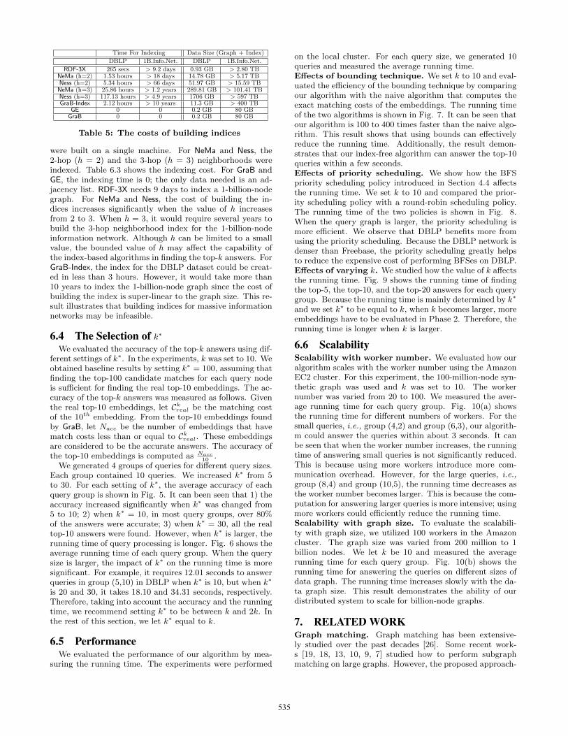
Table 5: The costs of building indices

were built on a single machine. For NeMa and Ness, the2-hop (h = 2) and the 3-hop (h = 3) neighborhoods wereindexed. Table 6.3 shows the indexing cost. For GraB andGE, the indexing time is 0; the only data needed is an ad-jacency list. RDF-3X needs 9 days to index a 1-billion-nodegraph. For NeMa and Ness, the cost of building the in-dices increases significantly when the value of h increasesfrom 2 to 3. When h = 3, it would require several years tobuild the 3-hop neighborhood index for the 1-billion-nodeinformation network. Although h can be limited to a smallvalue, the bounded value of h may affect the capability ofthe index-based algorithms in finding the top-k answers. ForGraB-Index, the index for the DBLP dataset could be creat-ed in less than 3 hours. However, it would take more than10 years to index the 1-billion-node graph since the cost ofbuilding the index is super-linear to the graph size. This re-sult illustrates that building indices for massive informationnetworks may be infeasible.

6.4 The Selection of k∗We evaluated the accuracy of the top-k answers using dif-

ferent settings of k∗. In the experiments, k was set to 10. Weobtained baseline results by setting k∗ = 100, assuming thatfinding the top-100 candidate matches for each query nodeis sufficient for finding the real top-10 embeddings. The ac-curacy of the top-k answers was measured as follows. Giventhe real top-10 embeddings, let Ckreal be the matching costof the 10th embedding. From the top-10 embeddings foundby GraB, let Nacc be the number of embeddings that havematch costs less than or equal to Ckreal. These embeddingsare considered to be the accurate answers. The accuracy ofthe top-10 embeddings is computed as Nacc

10.

We generated 4 groups of queries for different query sizes.Each group contained 10 queries. We increased k∗ from 5to 30. For each setting of k∗, the average accuracy of eachquery group is shown in Fig. 5. It can been seen that 1) theaccuracy increased significantly when k∗ was changed from5 to 10; 2) when k∗ = 10, in most query groups, over 80%of the answers were accurate; 3) when k∗ = 30, all the realtop-10 answers were found. However, when k∗ is larger, therunning time of query processing is longer. Fig. 6 shows theaverage running time of each query group. When the querysize is larger, the impact of k∗ on the running time is moresignificant. For example, it requires 12.01 seconds to answerqueries in group (5,10) in DBLP when k∗ is 10, but when k∗

is 20 and 30, it takes 18.10 and 34.31 seconds, respectively.Therefore, taking into account the accuracy and the runningtime, we recommend setting k∗ to be between k and 2k. Inthe rest of this section, we let k∗ equal to k.

6.5 PerformanceWe evaluated the performance of our algorithm by mea-

suring the running time. The experiments were performed

on the local cluster. For each query size, we generated 10queries and measured the average running time.Effects of bounding technique. We set k to 10 and eval-uated the efficiency of the bounding technique by comparingour algorithm with the naive algorithm that computes theexact matching costs of the embeddings. The running timeof the two algorithms is shown in Fig. 7. It can be seen thatour algorithm is 100 to 400 times faster than the naive algo-rithm. This result shows that using bounds can effectivelyreduce the running time. Additionally, the result demon-strates that our index-free algorithm can answer the top-10queries within a few seconds.Effects of priority scheduling. We show how the BFSpriority scheduling policy introduced in Section 4.4 affectsthe running time. We set k to 10 and compared the prior-ity scheduling policy with a round-robin scheduling policy.The running time of the two policies is shown in Fig. 8.When the query graph is larger, the priority scheduling ismore efficient. We observe that DBLP benefits more fromusing the priority scheduling. Because the DBLP network isdenser than Freebase, the priority scheduling greatly helpsto reduce the expensive cost of performing BFSes on DBLP.Effects of varying k. We studied how the value of k affectsthe running time. Fig. 9 shows the running time of findingthe top-5, the top-10, and the top-20 answers for each querygroup. Because the running time is mainly determined by k∗

and we set k∗ to be equal to k, when k becomes larger, moreembeddings have to be evaluated in Phase 2. Therefore, therunning time is longer when k is larger.

6.6 ScalabilityScalability with worker number. We evaluated how ouralgorithm scales with the worker number using the AmazonEC2 cluster. For this experiment, the 100-million-node syn-thetic graph was used and k was set to 10. The workernumber was varied from 20 to 100. We measured the aver-age running time for each query group. Fig. 10(a) showsthe running time for different numbers of workers. For thesmall queries, i.e., group (4,2) and group (6,3), our algorith-m could answer the queries within about 3 seconds. It canbe seen that when the worker number increases, the runningtime of answering small queries is not significantly reduced.This is because using more workers introduce more com-munication overhead. However, for the large queries, i.e.,group (8,4) and group (10,5), the running time decreases asthe worker number becomes larger. This is because the com-putation for answering larger queries is more intensive; usingmore workers could efficiently reduce the running time.Scalability with graph size. To evaluate the scalabili-ty with graph size, we utilized 100 workers in the Amazoncluster. The graph size was varied from 200 million to 1billion nodes. We let k be 10 and measured the averagerunning time for each query group. Fig. 10(b) shows therunning time for answering the queries on different sizes ofdata graph. The running time increases slowly with the da-ta graph size. This result demonstrates the ability of ourdistributed system to scale for billion-node graphs.

7. RELATED WORKGraph matching. Graph matching has been extensive-ly studied over the past decades [26]. Some recent work-s [19, 18, 13, 10, 9, 7] studied how to perform subgraphmatching on large graphs. However, the proposed approach-

535

20

40

60

80

100

5 10 15 20 25 30

Accuracy

(%)

Value of k∗

Query Size

(5, 10)

(4, 8)

(3, 6)

(2, 4)

(a) DBLP

0

20

40

60

80

100

5 10 15 20 25 30

Accuracy

(%)

Value of k∗

Query Size

(5, 10)

(4, 8)

(3, 6)

(2, 4)

(b) Freebase

Figure 5: The accuracy when varying k∗

0

5

10

15

20

25

30

35

40

5 10 15 20 25 30

Tim

e(secon

ds)

Value of k∗

Query Size

(5, 10)

(4, 8)

(3, 6)

(2, 4)

(a) DBLP

0

5

10

15

20

25

5 10 15 20 25 30

Tim

e(secon

ds)

Value of k∗

Query Size

(5, 10)

(4, 8)

(3, 6)

(2, 4)

(b) Freebase

Figure 6: The running time when varying k∗

100

101

102

103

104

(2,3) (2,4) (3,5) (3,6) (4,7) (4,8) (5,9)(5,10)

Tim

e(Secon

ds)

Size of Query Graph

w/o Bound GraB

(a) DBLP

100

101

102

103

(2,3) (2,4) (3,5) (3,6) (4,7) (4,8) (5,9)(5,10)

Tim

e(Secon

ds)

Size of Query Graph

w/o Bound GraB

(b) Freebase

Figure 7: Efficiency of bounding technique

05101520253035404550

(2,3) (2,4) (3,5) (3,6) (4,7) (4,8) (5,9)(5,10)

Tim

e(Secon

ds)

Size of Query Graph

GraB w/o PriorityGraB w/ Priority

(a) DBLP

1

2

3

4

5

6

7

8

9

10

(2,3) (2,4) (3,5) (3,6) (4,7) (4,8) (5,9)(5,10)

Tim

e(Secon

ds)

Size of Query Graph

GraB w/o PriorityGraB w/ Priority

(b) Freebase

Figure 8: Efficiency of priority scheduling

2

4

6

8

10

12

14

16

18

20

(2,3) (2,4) (3,5) (3,6) (4,7) (4,8) (5,9)(5,10)

Tim

e(Secon

ds)

Size of Query Graph

k=5k=10k=20

(a) DBLP

0

2

4

6

8

10

12

14

(2,3) (2,4) (3,5) (3,6) (4,7) (4,8) (5,9)(5,10)

Tim

e(Secon

ds)

Size of Query Graph

k=5k=10k=20

(b) Freebase

Figure 9: The running time when varying k

0

2

4

6

8

10

12

14

16

20 30 40 50 60 70 80 90 100

Tim

e(Secon

ds)

Worker Number

Query Size

(5,10)

(4,8)

(3,6)

(2,4)

(a) Varying worker num.

2

3

4

5

6

7

8

9

200 300 400 500 600 700 800 900 1000

Tim

e(Secon

ds)

Graph Size (Million Nodes)

Query Size

(5,10)

(4,8)

(3,6)

(2,4)

(b) Varying graph size

Figure 10: Scalability

es are not suitable for billion-node graphs due to expen-sive indexing costs. The graph-exploration-based subgraphmatching algorithm by Sun et al. [27] finds exact matches inbillion-node graphs. In contrast, our algorithm finds bothexact matches and similar matches.Top-k query. Top-k queries request the best-k answers fora given query [15]. The Threshold Algorithm and Fagin’sAlgorithm are commonly used to answer top-k queries [8].However, they require precomputing sorted lists to derivethe upper bounds and the lower bounds. For distributedgraph databases, the top-k graph query problems studied in[20, 11, 16] query for one unknown entity that are highlyrelevant to a given set of entities, but the problem we s-tudied considers the relationships among multiple unknownentities, which is more common in real life.RDF query. RDF queries are important for discoveringinformation on information networks. Some RDF query sys-tems [1, 23, 6] have been developed. These systems build so-phisticated indices on a single machine for query processing.In recent years, distributed RDF query systems [29, 14, 31]are proposed to support web-scale RDF graphs. Howev-er, the systems focus on finding the answers that exactlymatch queries. The flexible graph pattern queries have beenstudied in [25], which finds the answers similar to the RD-F queries. The approach stores RDF triples on HDFS [3]and answers the queries by repeatedly joining intermediateresults. In contrast, our approach does not produce a hugeamount of intermediate join results.Distributed graph computation. Since billion-node graph-s are increasingly common, distributed graph computationframeworks [32, 21, 22, 24] have been developed to supportgraph operations, such as computing PageRank scores andcomputing shortest paths. Although our system is imple-mented based on Piccolo [24], it can also be implemented onany other frameworks that can support breadth-first search.

8. CONCLUSIONIn this paper, we propose GraB, an index-free graph match-

ing algorithm for answering top-k queries on web-scale in-formation networks. Our approach provides meaningful an-swers via exact and similar matching. To obtain the an-swers quickly without indices, GraB utilizes a novel heuristicfor selecting the top candidates of query nodes and com-putes the bounds of matching scores to derive the top-kanswers instead of computing the exact matching scores. Adistributed system for the algorithm is proposed to allow s-calability. Our experiments demonstrate that the proposedapproach can efficiently answer queries on billion-node in-formation networks.

AcknowledgementsWe would like to thank Dr. Xiang Cheng for useful dis-cussion during the early stage of this work. This work ispartially supported by U.S. NSF grants CNS-1217284 andCCF-1018114, National Natural Science Foundation of Chi-na under Grants No. 61320106007, No. 61370207, No.61202449, No. 61300024, National High-tech R&D Programof China (863 Program) under Grants No. 2013AA013503,China Specialized Research Fund for the Doctoral Programof Higher Education under Grants No. 20110092130002,Jiangsu research prospective joint research project underGrants No. BY2012202, No.BY2013073-01, Jiangsu Provin-cial Key Laboratory of Network and Information Securityunder Grants No. BM2003201, Key Laboratory of Com-puter Network and Information Integration of Ministry ofEducation of China under Grants No. 93K-9. Jiahui Jinwas a visiting student at UMass Amherst, supported byChina Scholarship Council, when this work was performed.Any opinions, findings, conclusions or recommendations ex-pressed in this paper are those of the authors and do notnecessarily reflect the views of the sponsor.

536

References[1] Apache Jena. http://jena.apache.org/.

[2] DBLP.http://www.informatik.uni-trier.de/~ley/db/.

[3] Hadoop Distributed File System.http://hadoop.apache.org/.

[4] Linked Open Data.http://www.w3.org/wiki/SweoIG/TaskForces/

CommunityProjects/LinkingOpenData.

[5] T. Akiba, Y. Iwata, and Y. Yoshida. Fast exactshortest-path distance queries on large networks bypruned landmark labeling. In SIGMOD’13, pages349–360, 2013.

[6] M. Atre, V. Chaoji, M. J. Zaki, and J. A. Hendler.Matrix ”bit” loaded: a scalable lightweight join queryprocessor for rdf data. In WWW’10, pages 41–50,2010.

[7] J. Cheng, X. Zeng, and J. X. Yu. Top-k graph patternmatching over large graphs. In ICDE’13, pages1033–1044, 2013.

[8] R. Fagin, A. Lotem, and M. Naor. Optimalaggregation algorithms for middleware. J. Comput.Syst. Sci., pages 614–656, 2003.

[9] W. Fan, J. Li, S. Ma, N. Tang, Y. Wu, and Y. Wu.Graph pattern matching: From intractable topolynomial time. PVLDB, pages 264–275, 2010.

[10] W. Fan, X. Wang, and Y. Wu. Diversified top-k graphpattern matching. PVLDB, pages 1510–1521, 2013.

[11] Y. Fang, K. C.-C. Chang, and H. W. Lauw.Roundtriprank: Graph-based proximity withimportance and specificity. In ICDE’13, pages613–624, 2013.

[12] Google. “freebase data dumps”.https://developers.google.com/freebase/data.

[13] M. Gupta, J. Gao, X. Yan, H. Cam, and J. Han.Top-k interesting subgraph discovery in informationnetworks. In ICDE’14, pages 820–831, 2014.

[14] J. Huang, D. J. Abadi, and K. Ren. Scalable sparqlquerying of large rdf graphs. PVLDB, pages1123–1134, 2011.

[15] I. F. Ilyas, G. Beskales, and M. A. Soliman. A surveyof top-k query processing techniques in relationaldatabase systems. ACM Comput. Surv., 2008.

[16] J. Jin, S. Khemmarat, L. Gao, and J. Luo. Adistributed approach for top-k star queries on massiveinformation networks. In ICPADS’14, pages 9–16,2014.

[17] J. Jin, S. Khemmarat, L. Gao, and J. Luo. Queryingweb-scale information networks through boundingmatching scores. Technical report, 2015. http://rio.

ecs.umass.edu/mnilpub/papers/tech2015-jin.pdf.

[18] A. Khan, N. Li, X. Yan, Z. Guan, S. Chakraborty, andS. Tao. Neighborhood based fast graph search in largenetworks. In SIGMOD’11, pages 901–912, 2011.

[19] A. Khan, Y. Wu, C. C. Aggarwal, and X. Yan. Nema:Fast graph search with label similarity. PVLDB, pages181–192, 2013.

[20] S. Khemmarat and L. Gao. Fast top-k path-basedrelevance query on massive graphs. In ICDE’14, pages316–327, 2014.

[21] Y. Low, J. Gonzalez, A. Kyrola, D. Bickson,C. Guestrin, and J. M. Hellerstein. Distributedgraphlab: A framework for machine learning in thecloud. PVLDB, pages 716–727, 2012.

[22] G. Malewicz, M. H. Austern, A. J. C. Bik, J. C.Dehnert, I. Horn, N. Leiser, and G. Czajkowski.Pregel: a system for large-scale graph processing. InSIGMOD’10, pages 135–146, 2010.

[23] T. Neumann and G. Weikum. Rdf-3x: a risc-styleengine for rdf. PVLDB, pages 647–659, 2008.

[24] R. Power and J. Li. Piccolo: Building fast, distributedprograms with partitioned tables. In OSDI’10, pages293–306, 2010.

[25] P. Ravindra and K. Anyanwu. Scalable processing offlexible graph pattern queries on the cloud. InWWW’13 (Companion Volume), pages 169–170, 2013.

[26] D. Shasha, J. T.-L. Wang, and R. Giugno.Algorithmics and applications of tree and graphsearching. In PODS’02, pages 39–52, 2002.

[27] Z. Sun, H. Wang, H. Wang, B. Shao, and J. Li.Efficient subgraph matching on billion node graphs.PVLDB, pages 788–799, 2012.

[28] Y. Tian and J. M. Patel. Tale: A tool for approximatelarge graph matching. In ICDE’08, pages 963–972,2008.

[29] R. Verborgh, M. V. Sande, P. Colpaert, S. Coppens,E. Mannens, and R. V. de Walle. Web-scale queryingthrough linked data fragments. In LDOW’14, 2014.

[30] X. Yan, F. Zhu, P. S. Yu, and J. Han. Feature-basedsimilarity search in graph structures. ACM Trans.Database Syst., pages 1418–1453, 2006.

[31] K. Zeng, J. Yang, H. Wang, B. Shao, and Z. Wang. Adistributed graph engine for web scale rdf data.PVLDB, pages 265–276, 2013.

[32] Y. Zhang, Q. Gao, L. Gao, and C. Wang. Priter: Adistributed framework for prioritizing iterativecomputations. IEEE Trans. Parallel Distrib. Syst.,pages 1884–1893, 2013.

537