The spatial distribution of groundwater management policy impacts in the Republican River Basin of Colorado R. Aaron Hrozencik. Dale Manning, Jordan Suter, Chris Goemans Department of Agricultural and Resource Economics, Colorado State University

Ryan Bailey Department of Civil and Environmental Engineering, Colorado State University

[Preliminary Draft, please do not circulate]

Abstract

Groundwater is a critical input to agricultural production across the globe. Current groundwater pumping rates frequently exceed recharge, often by a substantial amount, leading to groundwater depletion and declines in agricultural profits over time. As a result, many regions reliant on irrigated agriculture have proposed policies to manage groundwater use. Even when gains from aquifer management exist, there is little information about how policies affect producers sharing the resource. In this paper, we investigate the variability of groundwater management policy impacts across heterogeneous agricultural producers. To explain these impacts, we develop a hydroeconomic model that captures the important role of well capacity, productivity of water, and weather uncertainty. We use the model to simulate the impacts of groundwater management policies on producers in a groundwater basin in Colorado and compare outcomes to a no-policy baseline. The management policies considered include a pumping fee, a quantity restriction, and an irrigated acreage fee. We find that well capacity, soil type, and well density affect policy impacts but in ways that can qualitatively differ across policy type. Because of the spatial distribution of these hydrologic and agronomic factors, model results have important implications for the distributional impacts and political acceptability of groundwater management policies.

1

1. Introduction

Groundwater accounts for 42% of global water supplies utilized to support irrigated agricultural production [Döll et al., 2012]. Much of this groundwater use utilizes aquifers that are pumped at rates that exceed natural recharge, leading to groundwater depletion over time [Famiglietti et al., 2011; Scanlon et al., 2012]. A changing global climate is predicted to exacerbate aquifer depletion as increased variability in precipitation induces further exploitation of groundwater resources to meet growing agricultural water demands [Vörösmarty et al., 2000]. Depletion of these scarce groundwater resources is a major concern in assuring future global food security and resilience to changes in climate. Addressing aquifer depletion concerns requires groundwater management policies that balance the short-run economic costs of reduced water use with the benefits of long-run water availability.

Despite growing interest in aquifer management [Little, 2009], the distribution of the costs and benefits of groundwater management policies across space and time remains unclear. In this paper, we investigate how spatial and temporal variation in both aquifer characteristics and agricultural production conditions affect the impact of specific groundwater management policies though the use of a spatially explicit hydroeconomic modeling framework. The model is applied to the Colorado portion of the Republican River Basin and incorporates producer planting and groundwater use decisions as economic choices that account for spatial variation in both agronomic and climate conditions. Importantly, the model captures the importance of well capacity as a main driver of how changing aquifer conditions affect producer water use and profitability. Understanding the distributional impacts of groundwater management policies informs policy development and implementation that appropriately balances efficiency gains with distributional impacts across both space and time.

Hydroeconomic models are the primary tool utilized to evaluate the costs and benefits of groundwater management policy alternatives [Harou et al., 2009]. Early hydroeconomic research utilized single cell ‘bath-tub’ aquifer models that assume homogeneity of hydrologic characteristics across space [Gisser and Sanchez, 1980; Allen and Gisser, 1984; Zimmerman, 1990]. More recent hydroeconomic literature recognizes the importance of modeling spatially explicit aquifer responses to pumping [Blanco-Gutiérrez et al., 2013; Esteve et al., 2015; Mulligan et al., 2014; Guilfoos et al., 2013; 2016] while accounting for human behavioral responses to changing aquifer conditions [Noel and Cai, 2017]. These models do not, however, account for heterogeneity in both aquifer and agricultural production conditions across groundwater users and time. In particular, previous literature does not capture the complex non-linear impacts of aquifer depletion on agricultural water use and profit induced by groundwater depletion, especially due to changes in well capacity over time.

Most existing economic models of groundwater use assume the primary avenue connecting changes in hydrology and groundwater use decisions is the vertical distance required to pump groundwater in a given location of the aquifer. In this formulation, the costs of groundwater depletion are limited to the additional energy costs required to pump groundwater an increased vertical distance. Recent literature, however, argues that well capacity has a larger impact on groundwater use decisions than depth to groundwater [Foster et al., 2015]. Well capacity, i.e. the

2

allowable yield of a well (‘well yield’), represents a physical constraint imposed by the location of the pump inside the well and the local saturated thickness within the aquifer. This constraint limits the volume of groundwater that can be pumped within a unit of time. Declines in well capacity limit an irrigator’s ability to meet daily crop water requirements and have been shown empirically to diminish the productivity of groundwater irrigation [O’Brien et al., 2001; Peterson and Ding, 2005; Lamm et al., 2007; Colaizzi et al., 2009; Foster et al., 2014], leading to non-linear changes in irrigated land and producer profits [Foster et al., 2015]. In this paper, we demonstrate that failing to account for constraints on well capacity significantly alters the predicted impacts of groundwater management policies.

This paper is the first to implement a basin-wide hydroeconomic model that incorporates economic behavior that is driven by changes in well capacity and changes in depth to groundwater. The paper contributes to the groundwater management literature in three important ways. First, we develop a novel methodology for deriving changes in well capacity using output from a spatially explicit groundwater model calibrated and tested for the Republican River Basin [RRCA, 2007]. This allows us to fully account for the dynamic feedbacks that exist between aquifer and economic systems compared to previous research where feedback is limited to changes in depth to groundwater. Second, we account for heterogeneity in demand for groundwater across irrigators and time by estimating well and crop-specific production functions that capture the breadth of agricultural production conditions observed in the study area. The water-yield production functions are generated by integrating geospatial data on soil, climate, and hydrological characteristics with an agronomic model [Steduto et al., 2009; Foster, 2017] and allow us to capture variation in water and land productivity across space. Third, we utilize a two-stage economic decision-making model to account for weather uncertainty in planting and water use decisions. This rigorous decision framework captures the role of planting decisions in driving the demand for water while highlighting the increased risk faced by producers as groundwater becomes further depleted.

Our policy analysis focuses on three differing groundwater management alternatives: a pumping fee, an irrigated acreage fee, and a quantity restriction. Following previous research [Guilfoos et al., 2016], the analysis evaluates viable, implementable policies, rather than attempting to identify economically optimal policy instruments. Model results demonstrate the heterogeneity in policy impacts while highlighting the importance of well capacity in predicting both baseline and policy scenario water use and agricultural profitability.

The remainder of the paper is organized as follows. A background and literature section introduces the study area and situates this research within the groundwater economics literature. We next explain the methodology of the hydroeconomic model development, emphasizing how differing model components are utilized and integrated into the modeling framework. We then present the results generated by the hydroeconomic model regarding how alternative management policies differentially influence heterogeneous groundwater users. We then discuss results and conclude by describing the implications of the results for future hydroeconomic modeling and groundwater management policies in practice.

3

2. Background and Literature Review

The High Plains aquifer is the largest aquifer in North America, underlying over 450,000 km2 from northern Texas to eastern Colorado and north to South Dakota. Large-scale, groundwater-fed irrigated agriculture supported by the High Plains aquifer began after the drought of the 1930’s [Robson and Banta, 1995]. Developments in pumping and irrigation technology and the availability of low-cost energy allowed further expansion of irrigated agriculture in the post-war era, transforming the High Plains from the “Great American Desert” to the “breadbasket of the world” [Sanderson and Frey, 2014].

This paper focuses on the Republican River Basin of eastern Colorado (henceforth ‘the Basin’) where agriculture accounts for over 92% of all groundwater extractions [Robson and Banta, 1995] (see Figure 1 for location of the Basin in the High Plains Aquifer). The Basin comprises 18,000 km2, nearly the area of the state of New Jersey [CDWR, 1996]. The total population of the Basin in 2010 was 35,415, with a density of less than 5 people per square mile [US Census Bureau, 2010]. There are over 3,000 wells permitted for irrigation purposes in the Basin and the agricultural production they support plays an important role in the local economy, boosting employment in both agricultural and non-agricultural sectors [Thorvaldson and Pritchett, 2006].

Figure 1. Map of Republican River Basin within the High Plains Aquifer

Given the importance of groundwater for the rural economy, there exists growing concern among producers and community members in the Basin regarding the depletion of the shared groundwater resource. The governance of groundwater resources is split between state entities and seven local groundwater management districts [Colo. Rev. Stat. (CRS) § 37-90-102]. There exists considerable heterogeneity in saturated thickness and well capacity across groundwater

4

users in the study area. Figure 2 describes the distribution of well capacity across permitted groundwater wells illustrating the degree of heterogeneity in access to groundwater that exists.

Figure 2. Histogram of well capacities in the Republican River Basin of Colorado

Rather than focusing on the identification of economically optimal groundwater policies, our analysis assesses the impacts of specific policies under consideration by local groundwater management districts. In particular, we separately evaluate the impacts of a pumping fee, an irrigated acreage fee, and a quantity restriction that are applied uniformly throughout the Basin. The hydroeconomic modeling framework that we develop is capable of accounting for the agronomic and hydrologic variation across the Basin to assess the spatial impacts of management policies.

An extensive body of literature uses hydroeconomic models to examine how hydrologic and economic systems interact and to evaluate the costs and benefits of groundwater management policies. Gisser and Sanchez’s [1980] – hereafter G&S – notable conclusion that gains to groundwater management are negligible served as a starting point for an active debate within the literature regarding the merits and efficient design of groundwater management policies. Research building on G&S relaxes many of the restrictive assumptions employed in their original work to test the robustness of their findings. Allen and Gisser [1984] demonstrate that the G&S result does not depend on the specification of the water demand function. Similarly, Feinerman and Knapp [1983] show that although model parameters influence gains to management, the benefits remain relatively small. Brill and Burness [1994] show that the best potential for gains associated with management occur in cases where the discount rate is low, well capacity decreases with aquifer depth, and water demand grows over time. This early

5

literature utilized single-cell, ‘bath-tub’ aquifer models which assume that the aquifer responds uniformly and instantaneously to groundwater pumping.

Research by Brozovic et al. [2010] questions the applicability of single-cell models in accurately capturing the spatial externality of groundwater pumping. Using results from the physically-based Theis [1935] solution that simulates changes in groundwater head in surrounding areas due to pumping, Brozovic et al. [2010] suggest that for large aquifers, single-cell models may significantly underestimate pumping externalities compared to spatially-explicit aquifer models. In response, more recent research utilizes spatially explicit hydrologic models [Esteve et al., 2015; Mulligan et al., 2014; Guilfoos et al., 2013; 2016]. These studies highlight the importance of aquifer heterogeneity in understanding groundwater use decisions and the impacts of management policies, although the groundwater modeling is often limited to water balance accounting or applying simple flow equations between adjacent aquifer regions.

To account for the spatially explicit nature of groundwater availability, hydroeconomic models have utilized a suite of groundwater flow simulation models. The basis for the majority of these models is Darcy’s Law, a momentum equation that describes water flow through a porous medium based on a head gradient and hydraulic conductivity [Klute, 1965]. Whereas some studies have used Darcy’s Law by itself to model water flows from location to location within an aquifer due to pumping [Guilfoos et al., 2013; 2016], others use physically-based spatially-distributed groundwater models that imbed Darcy’s Law into a conservation of mass statement to account for head fluctuation in a multi-dimensional, heterogeneous unconfined aquifer system. For example, several hydroeconomic models [Kuwayama and Brozović, 2013; Mulligan et al., 2014; Kahil et al., 2016; Noel and Kai, 2017] utilize regionally calibrated versions of MODFLOW [Harbaugh, 2000]. In particular, Kahil et al. [2017], Mulligan et al. [2014], and Kuwayama and Brozovic [2013] have utilized the RRCA MODFLOW model employed in our analysis [RRCA, 2007]. These hydroeconomic models account for the spatial heterogeneity of groundwater availability over time, but, by themselves, do not fully account for the complex variation in groundwater demand across space.

One important component of groundwater demand that has recently received attention in hydroeconomic modeling is well capacity [Peterson and Ding, 2005; Foster et al., 2014; 2015]. Foster et al. [2014] demonstrate that groundwater depletion-induced decreases in well capacity can generate large reductions in irrigated acreage, as an irrigator anticipates constrained intra-seasonal groundwater availability. Results suggest that well capacity is an important factor in defining the dynamic feedbacks that exist between economic and hydrologic systems. Despite this, the hydroeconomic literature has yet to incorporate well capacity into integrated modeling at a basin scale. Rather, the literature has followed the methodology outlined in G&S that links hydrologic and economic systems via changes in pumping costs induced by increased head lift requirements as groundwater levels decline [Esteve et al., 2015; Mulligan et al., 2014; Guilfoos et al., 2013; 2016]. Foster et al. [2015] demonstrate that well capacity has a larger impact on groundwater demand than depth to groundwater and pumping costs. They do not, however, illustrate how limited capacity dynamically alters groundwater use and decision-making on a basin-wide scale. The spatially-explicit hydroeconomic modeling framework that we develop uses the results from Foster et al. [2015] as a starting point in linking the planting and irrigation

6

decisions of heterogeneous groundwater users to evolving aquifer conditions via both well capacity and depth to groundwater.

Figure 3 illustrates the relationship between both well capacity and depth to groundwater in the Basin over the period 2011-2015. Consistent with Foster et al. [2015] well capacity appears to be a stronger predictor of pumping over the range of hydrologic conditions observed throughout the region.

Figure 3. Plots of the relationship between reported groundwater pumping and well capacity (left) and depth to groundwater (right) in the Republican River Basin of Colorado. Well capacity data were obtained from results of recent well capacity tests mandated by the Republican River Compact Agreement. Well-level depth to groundwater data were obtained from a USGS geospatial dataset (Flynn et al., 2009). The r2 statistics reported come from two separate linear regression models relating the log of mean groundwater pumping to the log of well capacity or log of depth to groundwater.

The r2 statistics reported in Figure 3 demonstrate that depth to groundwater does not capture the observed variation in groundwater pumping decisions, which stands in contrast to the strong statistical relationship between well capacity and variation in pumping decisions. These empirical results, combined with the connection between groundwater depletion and diminished well capacities [Hecox et al., 2002; Konikow and Kendy, 2005], highlight the importance of including well capacity as a dynamic feedback linking economic and hydrologic systems.

Previous literature utilizes groundwater demand functions that are independent of crop choice, soil type, growing season weather realizations, the amount of land irrigated, and well capacity [Gisser and Sanchez, 1980; Brill and Burness, 1994; Blanco-Gutiérrez et al., 2013; Mulligan et al., 2014]. These hydrologic and agronomic attributes, however, are important factors in determining groundwater demand as water needs and crop yields differ across crop and soil types [Hank, 1983; KIRDA, 1999], realized weather outcomes [Blaney and Criddle, 1962; Schlenker and Roberts, 2006], well capacity, and total irrigated acreage [Foster et al., 2014]. Guilfoos et al. [2016] recognize this shortcoming and evaluate how heterogeneous groundwater demand influences irrigator welfare gains under specific aquifer management scenarios. Results suggest that individual gains are highly correlated with the spatial distribution of groundwater pumping demand. Nevertheless, heterogeneity in groundwater demand and crop choice are assumed constant across time and do not depend on evolving aquifer conditions that determine planting

7

and pumping decisions. Our model accounts for the spatially explicit nature of water use through the use of water-yield production functions that capture the heterogeneity in irrigated agricultural production conditions to predict well-level groundwater demand.

Planting decisions are an important determinant of well-level groundwater demand as irrigation requirements differ across crops [Hank, 1983; Pfieffer and Lin, 2014] and diminished well capacity can induce irrigators to decrease irrigated acreage [Foster et al., 2014]. Previous literature models planting choices by utilizing long-run groundwater demand functions that implicitly account for changes in production, technology, and crop choice [Gisser and Sanchez, 1980; Brill and Burness, 1994; Guilfoos et al. 2013; Guilfoos et al., 2016]. However, this approach does not fully capture the dynamic interaction that occurs between evolving aquifer conditions and irrigators’ yearly planting decisions. Mulligan et al. [2014] model crop choice-specific groundwater demand as a function of changing pumping costs and fixed crop yield estimates. But their methodology does not account for the uncertainty regarding growing season weather outcomes that irrigators experience when making planting decisions before the realization of growing season weather. Our irrigation decision-making framework surmounts this challenge by explicitly modeling planting decisions made under growing season weather uncertainty, similar to Sunantara and Ramírez [1997]. Our method allows irrigators to respond to evolving aquifer conditions by adjusting along both intensive (water applied per acre) and extensive (number and type of irrigated acres planted) margins.

3. Methods

In this section, we describe the three primary components of our hydroeconomic modeling framework, which is designed to capture the spatial variation in groundwater management impacts. We begin with a description of the economic model that determines groundwater use. Next, we describe the process by which the production functions used in the economic model are generated using the agronomic model AquaCrop [Steduto et al., 2009]. We then describe the groundwater model and how it allows the groundwater use decisions to interact with aquifer characteristics. We conclude the section with a discussion of how the three model components are dynamically integrated.

3.1 Economic Model

The economic model assumes that a two-stage decision-making process determines annual groundwater use decisions, with an individual well, indexed by i=1,2,3 , … I , serving as the decision-making unit [Manning et al., 2017]. In the first stage, planting decisions that maximize expected profit are made based on a known distribution of potential weather outcomes. In the second stage, a particular weather outcome is realized and the producer is assumed to make a profit maximizing irrigation decision, conditional on the crop mix chosen in stage one.

In the first stage, the number of acres planted in crop j ,with j=1,2,3.. J , is determined for each well before weather is realized for the growing season. The first-stage objective function is

8

maxA ij

E ¿¿

s . t .∑j=1

J

A ij≤ A , ∑j=1

J

A ij x ij≤W ∀ i=1 , …. I ,(1)

where f j is the per-acre water-yield production function for crop j, which depends on the amount of water applied per acre, x ij. An agronomic model, described in the next section, is used to generate crop-specific production functions that differ based on hydrologic and agronomic characteristics. c¿ is well capacity and is a function of hydrologic characteristics of the aquifer at well location i in year t ,ρ¿. θ¿ is a random variable representing weather for well i in year t , and

ϕi includes well-specific soil characteristics. Importantly, ∂ f∂ c

>0 and ∂2 f∂ c∂ x

>0, which implies

that reductions in capacity result in lower yield of crop j. Finally, crop yields per acre depend on the number of acres planted in each crop, Aij, because when fewer acres are irrigated, more water can be delivered per acre of irrigated land. The per acre cost of planting and harvesting crop j is given by h j. The cost of pumping a unit of groundwater for well i, μ (d¿), is a function of the

depth to groundwater, d¿ at well i in time t. It is assumed that ∂ μ∂ d

>0, which reflects that energy

costs increase as depth to groundwater increases. A is a constraint on the maximum amount of land an irrigator can plant with irrigated or dryland crops. Groundwater management policy parameters are included in the formulation of the economic model to generalize the model to an evolving policy landscape. Specifically, ωis a fee paid per acre of irrigated land, τ is a fee levied per unit of groundwater and W is a constraint that limits the total volume of groundwater a well can pump within a season.

At the time of planting, the weather outcome, θ¿, is a random variable. In stage two, θ¿ is realized and an irrigation decision for each irrigated crop planted is made such that:

maxx ij

[∑j∈ Jp j Aij f j (x ij ; c¿ ( ρ¿ ) ,θ¿ , ϕ i , Aij )−A ij x ij ( μ (d¿ )+τ )] (2)

s . t .∑j=1

J

A ij x ij ≤ W

In the second stage, Aij represents the planting decision made in stage one, which is fixed in stage two, and the producer chooses a volume of water to apply per acre of each crop, x ij. The model is solved using backward recursion, which generates profit maximizing irrigation decisions at each well for all possible weather realizations. Substituting profit maximizing irrigation decisions for all weather realizations into Equation 1 provides the information needed to solve for the stage one planting decision that maximizes expected profits. This calculation is made at each well, generating profit maximizing planting and irrigation decisions for specific weather realizations, climatic zones, soil types, well capacities, and depth to groundwater.

9

The economic parameters used in the model are drawn from several sources. The costs of planting and harvesting crop j, h j, are estimated using crop enterprise budgets [Colorado State Extension, 2013]. The model includes the following crops - irrigated corn, dryland corn, irrigated wheat, and dryland wheat, which represent more than 90% of total acreage planted in the Basin [USDA Colorado Agricultural Statistics, 2014]. The function μ (d¿ ) is parameterized such that the average well’s volumetric pumping cost equals the pumping costs reported in enterprise budgets for northeastern Colorado [Colorado State Extension, 2013]. Also, it is assumed that μ (0 )=0. The model utilizes 15 years of USDA data on national, marketing year crop prices to estimate average output prices which we assume are constant across the simulation period [USDA NASS, 2017]. Finally, the output price of a given crop does not depend on whether it is irrigated or not. Table 1 summarizes the price and cost parameters used for the well-level optimization problem.

Table 1. Parameters used in economic model

Output PricesCorn 5.24 $/BushelWheat 6.20 $/Bushel

Per-Acre Planting and Harvesting CostsIrrigated Corn 547.86 $/AcreIrrigated Wheat 300.92 $/AcreDryland Corn 226.51 $/AcreDryland Wheat 147.93 $/Acre

Pumping Costs μ (d¿ ) 0.04 d¿ $/Acre Foot

3.2 Agronomic Model

The well-specific water-yield production functions, f j ( x ij ;c¿ ( ρ¿ ) , θ¿ , ϕi , A ij), used in the economic model are generated using AquaCrop [Steduto et al., 2009]. The water-driven plant growth model simulates crop biomass accumulation at a daily time step taking soil, weather, agronomic, hydrologic, and management parameters as inputs. See Steduto et al. [2009] for a complete review of the agronomic principles underlying AquaCrop. We utilize an updated, open-source version of AquaCrop developed by Foster [2017] that permits the model to accept well capacity and the amount of land irrigated as inputs to constrain irrigation scheduling and the productivity of water.

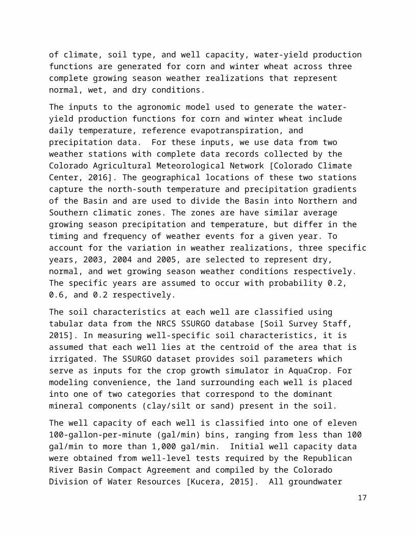
To generate water-yield production functions that capture the breadth of agricultural production conditions in the Basin while maintaining model tractability, we classify each well by climatic zone, soil type, and well capacity. For each unique combination of climate, soil type, and well capacity, water-yield production functions are generated for corn and winter wheat across three complete growing season weather realizations that represent normal, wet, and dry conditions.

10

The inputs to the agronomic model used to generate the water-yield production functions for corn and winter wheat include daily temperature, reference evapotranspiration, and precipitation data. For these inputs, we use data from two weather stations with complete data records collected by the Colorado Agricultural Meteorological Network [Colorado Climate Center, 2016]. The geographical locations of these two stations capture the north-south temperature and precipitation gradients of the Basin and are used to divide the Basin into Northern and Southern climatic zones. The zones are have similar average growing season precipitation and temperature, but differ in the timing and frequency of weather events for a given year. To account for the variation in weather realizations, three specific years, 2003, 2004 and 2005, are selected to represent dry, normal, and wet growing season weather conditions respectively. The specific years are assumed to occur with probability 0.2, 0.6, and 0.2 respectively.

The soil characteristics at each well are classified using tabular data from the NRCS SSURGO database [Soil Survey Staff, 2015]. In measuring well-specific soil characteristics, it is assumed that each well lies at the centroid of the area that is irrigated. The SSURGO dataset provides soil parameters which serve as inputs for the crop growth simulator in AquaCrop. For modeling convenience, the land surrounding each well is placed into one of two categories that correspond to the dominant mineral components (clay/silt or sand) present in the soil.

The well capacity of each well is classified into one of eleven 100-gallon-per-minute (gal/min) bins, ranging from less than 100 gal/min to more than 1,000 gal/min. Initial well capacity data were obtained from well-level tests required by the Republican River Basin Compact Agreement and compiled by the Colorado Division of Water Resources [Kucera, 2015]. All groundwater wells are assumed to irrigate using a center pivot irrigation system, which is the irrigation method that accounts for more than 85% of all irrigated land in Colorado [USDA Farm and Ranch Irrigation Survey, 2013]. Furthermore, we assume wells can potentially irrigate a 130 acre circle of land. This is the modal area irrigated in the study area and corresponds to a full circle of irrigated land on a quarter-quarter section of land [Bauder et al., 2004]. Planting decisions for specific crops are discretized into quarter circle (32.5 acres) increments based on discussions with producers in the study area regarding cropping management units.

An irrigation management schedule specifies the frequency and amount of irrigation applied throughout the growing season and is determined by a soil moisture target (SMT) that establishes a percentage of the soil’s available water capacity (AWC) between the permanent wilting point and field capacity. If the AWC falls below the SMT target on a given day, then an irrigation event is triggered to increase the AWC back to that season’s target. However, an irrigation event’s capability to meet a deficit between current AWC and the SMT is constrained by well capacity and the number of acres irrigated. We vary the SMT for a given combination of crop, soil type, well capacity, weather realization, amount of irrigated land, and climatic zone to relate crop yields to seasonal water application rates for all potential combinations of weather, well characteristics, and land types. This produces a yield and water volume for each crop model run.

Piece-wise functions are generated to fit the crop yield and water application data generated by AquaCrop. We assume that yield response to irrigation is constant below the minimum yield and above the maximum yield predicted. In between the bounds defined by minimum and maximum yield, a second-order polynomial is fit to the remaining yield and irrigation application data

11

utilizing a least-squares algorithm. This data-generating and function-fitting process is repeated for all possible combinations of crop (2), climatic zone (2), well capacity (11), soil type (2), weather realization (3) and irrigated acreage (4) to create 1,056 unique water-yield production functions that capture the heterogeneity in agricultural production conditions observed in the Basin. The appropriate production functions are then assigned to each specific well in the Basin by matching on observable climatic zone, well capacity, and soil type characteristics. As an illustration, Figure 3 presents estimated production functions for two different well capacities across two acreage decisions, demonstrating how the productivity of water for low capacity users differs based on the amount of land irrigated. Note that when the full circle is irrigated with low well capacity, water productivity is very low compared to higher capacity. On the other hand, if only a quarter of a circle is planted, the low and high capacity wells perform similarly.

Figure 4. Example of water-yield production functions for corn planted on sandy soil in the northern climatic zone during a normal weather growing season for wells with capacity of 300 (left) and 1,000 gal./min. (right)

3.3 Hydrologic Model

The hydrologic model consists of a groundwater MODFLOW model that simulates spatially-varying hydraulic head and streamflow depletion due to groundwater pumping; recharge from rainfall events, irrigation events, and stream and irrigation canal seepage; and evapotranspiration from the groundwater and from phreatophytes. The model utilizes a single layer to define the aquifer between the ground surface and the bedrock, with the Basin discretized into finite difference cells of 1 mi2, with temporal discretization of monthly stress periods and bi-monthly time steps. The model is run from 1918 to 2006, with results tested against groundwater levels from monitoring wells (350,233 water level records from 10,835 different sites) and baseflow in streams. Simulated cell-by-cell water table elevation for the year 2000 is shown in Figure 5 for the Basin, along with the pumping wells located within the Colorado portion of the Basin.

12

Figure 5. Water table elevation (ft above mean sea level) for each 1 mi2 grid cell of the Basin for the year 2000, as simulated by the RRCA MODFLOW model. The pumping wells in Colorado used in this study are also shown.

The economic model is linked to hydrologic conditions through changes in well-level pumping capacities and depth to groundwater. The Republican River Compact Agreement [RRCA] MODFLOW hydrologic model [RRCA, 2007; Harbaugh et al., 2000] is used to account for the impacts of groundwater pumping for irrigation on aquifer levels and future well capacities simulating spatially-variable hydraulic head for the 1918-2005 time period on monthly stress periods, with two time steps for each stress period. The horizontal discretization of the model is one mile by one mile, with one layer for the aquifer. The model incorporates groundwater pumping, evapotranspiration, recharge from rainfall, groundwater and surface water irrigation, and canal and stream seepage. For model simulations moving forward, the original groundwater pumping volumes are replaced with the result of the economic model decisions described in section 3.1. Groundwater head data throughout the Republican River Basin calibrated the RRCA model [RRCA, 2007].

Changes in well capacity over time are determined by first calculating the allowable pumping rate (Qallow) for each well, defined as the pumping rate (ft3/day), that can be applied throughout the subsequent year’s growing season without causing the water table within the immediate vicinity of the well to fall below the well’s pump. The allowable pumping rate, Qallow, is determined from the equation

(3)

where SC (ft2/day) is the specific capacity for the pumping well and sallow (ft) is the allowable drawdown that can occur at the well, defined by the difference between the head level at the end of the year (last time step in December) and the pump level, which is assumed to be 10 ft above the aquifer bottom. SC for each well is determined using relationships between the monthly pumping rate, Q, and resulting drawdown, s (based on the hydraulic head at the beginning of each year), as simulated by the 1918-2000 MODFLOW model simulation. Examples of this relationship are shown in Figure 6 for two example pumping wells, with values of Q and s coming from each of the 996 months of the MODFLOW output. Assuming a linear relationship between Q and s, the SC for each well is found by dividing the maximum pumping rate during

13

the 1918-2000 simulation by the associated drawdown s (see circled data point on each plot). Calculations also account for the occurrence of multiple pumps within a single MODFLOW grid cell, with the SC value divided by the number of pumps residing within the cell, based on the historical pumping rate assigned to each well.

Figure 6. Example Q-s relationships observed from RRCA model data

MODFLOW computes a cell-averaged hydraulic head value, and hence does not calculate the head value at the location of the pumping well. As simulations in this study are dependent on actual available groundwater, the drawdown values used to calculate SC must correspond to the maximum drawdown in the aquifer, i.e. within the immediate vicinity (< 1 ft) of the well borehole. This is accomplished by using the Dupuit-Thiem equation [Thiem, 1906] to relate the cell head value (hcell) to the head at the well borehole (hwell):

(4) (4)

where rw (ft) is the effective radius of the well borehole, rdist (ft) is the distance from the edge of the cell to the pumping well, and K is the horizontal aquifer hydraulic conductivity (ft2/day). In this study, rw is set to 1 ft for each well, and K is provided by the value specified for each MODFLOW cell. Equation 4 assumes steady, symmetric radial flow of groundwater towards a pumping well, and neglects any head loss due to local turbulence around the well.

14

The well-specific maximum allowable pumping estimates relate aquifer drawdown predicted by the RRCA model to pumping capacities. However, Qallow does not capture other well-level heterogeneity in pump characteristics and efficiency which also determine well pumping capacity. To address this omission, we utilize a dataset of recent well capacity tests conducted in our study area to serve as a benchmark for changes in pumping capacity through time. The most recent well capacity test results for a given well are used as that well’s initial pumping capacity. Yearly percent changes in a well’s Qallow are then used to scale the reported initial pumping capacity. This method allows our model to account for heterogeneity in well pump efficiency when predicting changes in well capacity through time.

3.4 Dynamic Model Integration

In this section, we describe how the hydroeconomic framework intergrates the economic, agronomic and hydrologic models to capture dynamic system feedbacks. The sequence of operations in the integrated model begins with the economic model predicting planting and groundwater use decisions in year one (t = 1) for each of the over 3,000 wells in the model. Initial well capacities are used to connect individual wells to the appropriate well capacity-specific production functions. Predicted groundwater pumping is then aggregated to the MODFLOW grid-cell and serves as the input into the year one (t = 1) iteration of the hydrologic model. Yearly grid-cell pumping volumes are assumed to be uniformly distributed throughout the growing season (May-August) and are utilized to rewrite monthly pumping volumes specified in the MODFLOW WELL package input file. 17% of recharge is assumed to come from irrigation return flows, while the remaining variation in recharge depends on precipitation levels.

MODFLOW output from year one provides input for the next iteration of the economic model (t = 2), updating well-level depth to groundwater and scaling initial well capacity based on changes in Qallow, as predicted by the hydrologic model. This iteration process is repeated throughout the simulation period, dynamically linking well-level groundwater pumping decisions in year t to aquifer conditions in year t + 1. See Figure 7 for a flow chart describing the sequence of operations defining the hydroeconomic model integration. The calculation of Qallow for each well is dependent on each well’s estimated specific capacity (SC), i.e. the ratio between pumping rate Q (ft3/day) and resulting drawdown (ft). The procedure for determining SC for each well and for calculating year-by-year Qallow for each well is described in Section 3.3.

15

Figure 7. Flow chart describe model integration process

Growing season weather realizations are also an important determinant of groundwater pumping decisions predicted by the economic model and aquifer recharge specified in the hydrologic model. For model tractability, we specify a 5-year cycle based on the assumed frequency of normal, dry, and wet growing seasons and repeat that cycle throughout the model simulation period (normal, wet, normal, dry, normal). From the producers’ perspective, each year has the same weather distribution as of the time of planting.

4. Results

We now present the results of the dynamic hydroeconomic model to examine both baseline and policy scenario water use and economic outcomes over space and time. We also explore the importance of well capacity changes in determining baseline and policy outcomes in a hydroeconomic model. In section 4.1, we present baseline hydroeconomic model results that demonstrate how well-level characteristics influence producer decision making and profitability, and how those characteristics interact with aquifer conditions to determine basin-wide outcomes. With no policy in place, we then simulate Basin-wide pumping, land use, and profitability over time using the linked model to establish a baseline scenario.

Next, in section 4.2, we explore the impact of water management policies. We begin by evaluating policy effectiveness within the static framework to understand how policy alternatives differentially impact water use and agricultural profits in the short run. Dynamic simulations with policies in place then allow us to investigate management policy impacts as well as the role of well capacity in influencing policy costs and benefits. We use simulation results to display

16

how policy costs and benefits are distributed across the Basin. Finally, an econometric model is utilized to characterize the wells that benefit most from each policy.

4.1 Baseline Model Analysis

We now focus on the behavior of the hydroeconomic system when no water management policy influences producer behavior.

4.1.1 Well capacity and producer decision making

We begin by examining static (initial year) outcomes based on output from the economic and agronomic models. By varying the price of water faced by a given producer type in the model, we simulate the how the water volume demanded responds to price. Figure 8 presents simulated inverse demand functions for three different well capacities on sandy (Panel A) and silt/clay (Panel B) soils and demonstrates how well capacity and depth to groundwater non-linearly impact expected groundwater demand. Demand by the high capacity wells is generally quite inelastic, reflecting only minor reductions in the quantity of groundwater extraction as the price of groundwater increases. At the lower well capacities, non-linearities arise as the price of groundwater increases due to impacts on planting decisions. For example, a well with 500 gal./min. capacity on sandy soil switches from irrigating 130 acres of corn to 97.5 acres of corn once the price of pumping an acre foot of groundwater exceeds $12. By not accounting for well capacity or explicitly modeling planting decisions, previous hydroeconomic models fail to capture the mechanisms driving irrigators’ responses to groundwater availability.

(A) (B)

Figure 8. Groundwater inverse demand functions (net marginal benefit) across soil types in northern climatic zone of study area. Variation in the price of groundwater could originate from variation in depth to groundwater and the resulting marginal pumping cost or equivalently a tax on groundwater use.

17

To illustrate how well capacities influence well-level profits, Figure 9 presents expected profit results for irrigated and dryland crops planted at a well, generated by the static modeling framework, across well capacities on sandy (Panel A) and silt/clay (Panel B) soils in the northern climate zone, holding depth to groundwater constant at 150 ft. We focus on expected profit, weighted according to the probabilities of a growing season being wet, dry, or normal as the irrigator chooses a planting decision to maximize expected profit. Differences in planting decisions are the primary source of large changes in expected profit as well capacity varies. Importantly, given the positive relationship between saturated thickness and well capacity, the results highlight how failing to account for well capacity mischaracterizes the relationship between groundwater depletion and agricultural profitability. Comparing panels A and B of Figure 9 demonstrates how heterogeneity in soil conditions also plays an important role in determining profitability. All else equal, crops planted on sandy soils require more irrigation water to achieve a given yield. This leads to lower expected profit on sandy soils, particularly as well capacity falls.

(A) (B)

Figure 9. Expected profit for differing well capacities and soil types in northern climate zone, assuming depth to groundwater is 150 ft.

4.1.2 Well capacity and dynamic baseline results

Incorporating evolving aquifer conditions over time allows us to explore how the inclusion of well capacity as a dynamic link between hydrologic and economic systems affects Basin-wide groundwater withdrawals, agricultural profits, and irrigated acreage. We begin this section by presenting the results of 50-year model simulations when well capacity changes over time and when it is held constant at initial levels, observed in recent well tests. All simulations use the same pattern of weather realizations, as described in section 3.

Based on the results depicted in Figure 10, ignoring well capacity changes results in much smaller decreases in basin-wide groundwater use (Panel A) and profit (Panel B) than when well capacity changes over time. Over time, as water productivity falls due to declines in well capacity, Basin-wide water use also falls, acting in some ways as a conservation incentive imposed by physical constraints. These results suggest that models that do not account for well

18

capacity lead to predictions that overstate water use over time and underestimate the impact of groundwater depletion on producer profits.

(A) (B)

19

(C) (D)

Figure 10. Simulated basin groundwater use (A), profit (B), irrigated land (C), and irrigated corn acreage (D), for baseline, ‘no policy’, scenario across two model specifications

Planting decisions are a key determinant of the relationship between aquifer conditions and agricultural profits because diminished well capacity constrains a producer’s ability to fully irrigate water intensive crops and therefore induces changes in cropping patterns. Baseline model results provided in Figure 10 for Basin-wide total irrigated acres (Panel C) and irrigated corn acres (Panel D) across both model specifications highlight how evolving aquifer conditions alter cropping patterns across time, shifting irrigated land away from water intensive crops (i.e., corn). Again, not accounting for the impact of well capacity leads to model results that underestimate the effects of groundwater depletion on cropping patterns and the amount of land irrigated. Decreases in the number of irrigated acres can have important economy-wide implications, as impacts from the agricultural sector are transmitted into the broader rural economy (Thorvaldson and Pritchett, 2006). Taken together, the results demonstrate the importance of well capacity changes in predicting profits, groundwater use, and land use.

4.2 Policy Analysis

For the policy analysis, we investigate the total and spatially explicit benefits and costs of three groundwater management policy types: a quantity restriction, a pumping fee and an irrigated acreage fee. Each policy is implemented uniformly across the study area. Revenues generated from fee-based policies are assumed to be aggregated by each of seven local management districts and redistributed via lump sum transfers to irrigators and are included in yearly profits.

4.2.1 Static policy analysis

We utilize the static economic model to evaluate the efficacy of each policy at reducing initial groundwater use from baseline amounts. Figure 11 illustrates how the three groundwater management policy types change initial, Basin-wide groundwater use and agricultural profits relative to the baseline, ‘no policy,’ scenario across a range of policy magnitudes. The figure demonstrates that the pumping fee achieves groundwater management objectives (percent decreases in basin pumping) with smaller impacts on basin-wide short-run agricultural profits compared to the other policies. The cost effectiveness of the pumping fee in generating groundwater conservation derives from its flexibility. Assigning a uniform price on groundwater throughout the Basin induces conservation in users with a low marginal product of water, while allowing users with a high marginal product of water to continue pumping. It also incentivizes both extensive and intensive margin responses. The other policies do not encourage conservation based on the marginal product of water. In fact, the irrigated acreage fee provides no incentive to reduce water along the intensive margin.

20

Figure 11. Static policy results of the cost of varying levels of water conservation under three alternative policies

4.2.2 Well capacity and management policy impacts

In this section, we evaluate water management policy impacts over a 50-year time horizon, again comparing constant well capacity results to variable well capacity results. The magnitude of each of the three policies is chosen such that it achieves an immediate 10% reduction in expected groundwater use from the baseline, ‘no policy’ scenario. Policy levels that achieve this goal are a pumping fee of $78 per acre-foot, a quantity restriction of 240 acre-feet per well, and an irrigated acreage fee of $185 per acre. While we present the results using policies that achieve a 10% initial reduction, the relative policy impacts across space and time are consistent across a wide range of reduction targets. In all cases, we assume a 5% discount rate to calculate the net present value (NPV) of profit under base and policy scenarios.

Table 2 presents summary statistics of estimated policy impacts. In the table, we present results of the model when well capacity can vary over time (Variable Capacity) and when well capacities are maintained at initial levels (Constant Capacity). This allows us to examine the importance of well capacity in assessing policy impacts within a hydroeconomic model. Observe that failing to account for well capacity overstates the negative impacts of the quantity restriction while understating the profit impacts of the fee based policies and the percentage of wells that benefit from groundwater management for all three policies. This suggests that ignoring well capacity misses an important external impact of groundwater pumping. Pumping groundwater not only increases the depth to water for neighboring wells, it also lowers the well capacities of other wells.

21

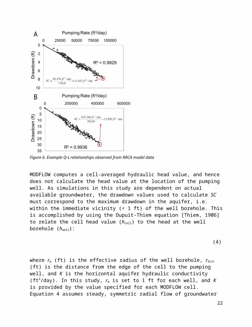
Table 2: Comparison of Basin-Wide Policy Impacts with Changing Well Capacity

Quantity Restriction -$58,621.85 -$70,908.91 -5.03% -5.89% 6.93 8.86 27.76 - 14.34% 6.12%($51,106.59) ($51,409.15) 0.045 0.041 5.054 6.145 32.669

Pumping Fee -$36,616.98 -$33,942.20 -3.14% -2.82% 5.22 5.32 24.01 - 22.52% 18.90%($80,855.7) ($74,199.6) 0.169 0.158 3.522 3.526 35.0198

Irrigated Acreage Fee -$46,962.03 -$33,146.51 -4.03% -2.75% 2.76 1.27 12.19 - 2.40% 0.80%($80,367.46) ($71,817.66) 0.162 0.155 3.623 2.547 25.339

Average Policy Benefit per Well

Policy Benefit, Percent of Baseline

NPV

Change in Saturated Thickness from Baseline

in year 50 (ft.)

Change in Well Capacity from Baseline

in year 50 (gal./min.)

Percent of Wells Benefiting from Policy

Variable Capacity

Constant Capacity

Variable Capacity

Constant Capacity

Variable Capacity

Constant Capacity

Variable Capacity

Constant Capacity

Variable Capacity

Constant Capacity

22

Ignoring changes in well capacity, tends to overstate the profit losses associated with the quantity restriction policy. Water use does not decrease in the baseline when capacity remains constant as it does when producers become increasingly capacity-constrained over time (see figure 10). Therefore, the impact of the quantity restriction is overstated when ignoring well capacity. Accounting for well capacity leads to a larger predicted decrease in profit from fee based policies because as capacity falls, the extra cost imposed by the policies induces further changes in planting decisions, making it costlier relative to the constant well capacity case.

Finally, note how policy impacts on saturated thickness and well capacity differ across hydroeconomic modeling specifications. For the quantity restriction and pumping fee not accounting for well capacity overstates the change in saturated thickness from the baseline compared to results generated with changing well capacity. Given how the inclusion of well capacity affects baseline water use, this result derives from the relative effectiveness of management policies in preserving saturated thickness from the baseline scenario. As producers become capacity-constrained in both policy and baseline scenarios the conservation induced by this constraint mutes the groundwater savings impacts of the policies. The opposite is true for the irrigated acreage fee where not accounting for well capacity understates policy impacts on saturated thickness. In this case, predicted conservation impacts increase due to the planting decisions induced by the inclusion of well capacity interacting with the policy instrument. Also, note how the policies generate differential impacts in terms of well capacity. While the pumping fee minimizes average policy costs it does not preserve well capacity as effectively as the quantity restriction. These results beckon further exploration of the characteristics of the physical system that determine the spatial distribution of policy impacts.

4.2.3 The spatial distribution of management policy impacts

In this section, the modeling framework is used to evaluate the dynamic impacts of each policy type. We focus our analysis on results that occur when well capacity varies over time. We employ the same assumptions as described above regarding the discount rate, and the spatial extent of policy implementation. Figure 12 provides a comparison of well-level net present value of profit (NPV) across the simulation period from the baseline scenario with NPV of profit under the three policy scenarios. Black points represent wells whose NPV of profits increases due to policy implementation. White points represent wells whose NPV profit decreases due to policy implementation. The spatial distribution of benefits and costs from differing management policies presented in Figure 12 indicates how heterogeneous aquifer and agricultural production conditions interact with differing policy instruments to determine management impacts. The spatially explicit results illustrate the concentration of policy impacts as well. In particular, note that the quantity restriction primarily generates gains for users in areas of the Basin with relatively less initial saturated thickness (mostly in the south). Wells with low saturated thickness and low well capacity use relatively less water in the baseline, making the quantity restriction less likely to bind. Furthermore, as well capacities drop over time, the quantity restriction binds for fewer wells.

23

The distribution of wells that benefit from the pumping fee is more uniform across space. This occurs because all wells face an incentive to reduce water use and they can adjust along the most cost-effective margins. The irrigated acreage fee, on the other hand, only incentivizes extensive margin adjustments and is costly to most wells in the Basin.

Figure 12. Net present value of well-level profits compared to baseline, ‘no policy,’ scenario.

4.2.4 The determinants of management policy impacts

To better understand the mechanisms driving heterogeneity in groundwater management policy impacts, we estimate the following model using an ordinary least squares regression assuming a linear relationship between net present value and the variables on the right hand side:

NPV ip=f ( ci 0 , d i 0, ϕ i , s i , ϑ i ; β , ϵi ) (5)

NPV ip is the net present value increase in well i’s profit for policy p compared to the net present

value profits in the no-policy baseline. c i 0 , di 0 and ϕi are as defined in Section 3 of the paper. ϑ i represents the climate zone for well i and si, the number of wells within two miles of well i. β is a vector of slope coefficients to be estimated and ϵ i is a random, mean-zero error term.

The estimation results in Table 3 illustrate how the specific model variables impact relative NPV under the quantity restriction, volume fee, and acreage fee. We employ a region-level fixed effects empirical model to account for unobserved heterogeneity across the study area. Several important lessons emerge from these results. First, note the impact of soil type on well-level profits. For the three policies evaluated, a sandy soil type negatively impacts well-level management policy benefits, supporting the intuition that crops planted on sandy soil require more irrigation water to be profitable. Thus, wells located on sandy soils are more likely to be negatively impacted by groundwater management policies than wells located on silt/clay soils.

24

Next, we examine the impact of well capacity across the policies. For the pumping fee and quantity restriction, a higher initial well capacity negatively affects the policies’ profit impact as wells with higher capacity are more likely to pump more groundwater in the baseline scenario (as seen in Figure 3) and experience profit losses due to the implementation of management policies. This means that wells with higher capacity reduce water use by more than those with low capacity and so the initial costs are higher. In fact, many low-capacity wells use less water than the quantity restriction even with no policy in place, meaning that they experience no policy cost while still receiving some benefits from neighboring wells conserving water over time.

Higher well capacity positively affects profit impacts under the irrigated acreage fee. Wells with high capacity are more profitable (as illustrated in Figure 9) and therefore they are more likely to pay the fee and plant irrigated crops than to not irrigate a given acre. Since the fee is redistributed lump-sum by local districts (and high capacity users cluster in space—see Figure 5), this policy does not harm high capacity users as much as the other two policies.

Table 3. Regression results predicting the changes in well-level profits of alternative management policies

Pumping Fee Quantity Restriction Irrigated Acreage FeeInitial Depth to Groundwater (ft.) -67.31452* -11.96577 70.28772**

(34.98) (15.7) (34.58)Initial Well Capacity (gal./min) -28.86203*** -61.19139*** 65.92623***

(4.53) (2.04) (4.48)Well Density (number of wells within 2 mile radius) 781.4429*** -79.00904 1065.809***

(262) (117.6) (258.99)Well Density X Hydraulic Conductivity Dummy 693.0205* 283.2009 311.2861(1 = High Hydraulic Conductivity, 0 otherwise) (419.37) (188.24) (414.56)Soil Type (1 = Sandy, 0 = Silt/Clay) -74791.77*** -37479.97*** -45145.54***

(3580.34) (1607.04) (3539.2)Intercept 103580.3*** 48736.86*** -48172.8***

(9801) (4399.36) (9688.74)

0.1445 0.3511 0.1259Observations 2,979 2,979 2,979Significance levels are indicated by *** 1%, ** 5%, * 10%

Model R2

Next, notice the impact of well density on policy impacts. Intuitively, wells that are located closer together inflict larger external impacts on nearby wells. Therefore, we expect groundwater management policies to benefit wells that are densely distributed. This is the case for the pumping fee and irrigated acreage fee. This result does not hold for the quantity restriction, however the coefficient estimate is not statistically significant.

The benefit of the pumping fee is decreased with a higher initial depth to water. For wells with shallow water, a higher price of water causes only intensive margin shifts in the quantity of water applied per acre. For wells with a high depth to water, the additional price induces a shift in planting decisions, leading to higher policy costs in the short run (see Figure 8). While the impact of the pumping fee depends on initial depth, the acreage fee impacts do not interact with

25

the depth to water as the policy does not target resource use along the intensive margin. Higher initial depth to water does not have a significant impact on policy benefits for the quantity restriction.

Finally, note the impact of well density interacted with a dummy variable for high hydraulic conductivity (HC). HC is a measure of the rate at which groundwater flows laterally, thus higher levels of HC increase the external impacts of neighbors’ pumping. The interaction between HC and well density captures how well density affects policy impacts conditional on a well having high HC. Intuitively, this interaction covariate should increase policy benefits and further elucidate the effect of well density. Results follow this intuition but are only statistically significant for the pumping fee.

Taken together, the results in Table 3 suggest that the spatial distribution of groundwater management policy impacts is in part determined by aquifer characteristics represented by initial well capacity and depth to groundwater, soil characteristics which influence the marginal productivity of irrigation water and the density of groundwater wells.

5. Discussion

The hydroeconomic model results illustrate how the costs and benefits of different groundwater management policies depend on interactions between aquifer and agricultural production conditions. In particular, while sandy soils consistently decrease policy benefits, other factors, including well capacity and well density have differing impacts across the policy types. Our results also highlight how the exclusion of well capacity as a dynamic feedback alters the extent and distribution of groundwater policy impacts.

Model results describing the distribution of policy impacts across space present a powerful tool to aid in targeting regions for groundwater management and formulating policies tailored to heterogeneous aquifer and agricultural production conditions. For example, a greater proportion of groundwater users in the southern part of the Basin benefit from the quantity restriction policy than users in the northern parts of the Basin. This relative difference in policy impacts derives from heterogeneous aquifer and agricultural production conditions. Many groundwater users in the southern part of the Basin have low initial well capacity, rendering the quantity restriction policy non-binding. However, these users still benefit as the quantity restriction limits the pumping of less capacity-constrained neighbors whose pumping imposes an external cost. By comparison, in the northern portion of the Basin, the quantity restriction generates sparse benefits as the relative abundance of groundwater and sandy soil conditions induce high levels of baseline pumping, making the quantity-based policy more binding. This example provides insight into how our model results can provide policymakers with valuable information about who will be impacted by different policy types. Policies can then be designed to minimize losses and so that policy impacts are distributed in a desirable way across the Basin.

Overall, the pumping fee generates positive benefits for more groundwater users than the quantity restriction or irrigated acreage fee, which follows the economic intuition that a fee-

26

based policy equates the marginal product of water to its marginal cost. Of course, this result is not guaranteed because equating the marginal benefit of water may not be optimal if marginal external pumping costs vary widely across the Basin. Despite the merits of the fee-based policy, it does not generate benefits for a majority of groundwater users which likely makes policy implementation challenging. Future research should investigate these redistribution mechanisms and analyze how they impact the viability of management policy implementation.

The results also illustrate the impact of not including well capacity on both the spatial distribution of policy impacts and the overall gains to management. Given the importance of well capacity in determining water use and profits and the ability of management policies to maintain capacity by encouraging conservation, it follows that not accounting for this dynamic feedback will miscalculate the gains of groundwater management. The exclusion of well capacity also alters the spatial distribution of policy impacts such that gains are primarily realized in regions with larger depth to groundwater where users stand to benefit from stabilized water table elevation. This stands in contrast to our results where the spatial distribution of impacts depends on both depth to water and the aquifer characteristics that determine well capacity. Models built without the inclusion of well capacity as a dynamic feedback may have limited policy relevance, particularly for distributional impacts, as they ignore an important factor that determines the extent and magnitude of management benefits and costs.

Finally, this paper does not purport that the policies evaluated constitute least-cost or optimal policies. Given the complex nature of aquifer resources and heterogeneity in external costs across wells, the optimal policy is well-specific and dynamically changing through time. The implementation of a policy of this sort would likely impose high administrative and enforcement costs. Rather than characterizing optimal policies, we follow Guilfoos et al. (2016) and focus our research efforts on viable, spatially uniform groundwater management policies. Future research efforts should relax some of our simplifying assumption about policy variation over space and time to investigate how the spatial scale of policy implementation influences policy impacts and the support for differing policies.

6. Conclusion

This paper develops a novel hydroeconomic modeling framework that contributes to the understanding of how aquifers and groundwater-fed irrigated agricultural systems interact through time and space. It is the first instance in the literature, that we are aware of, that includes well-level well capacity dynamics in a basin-scale integrated hydroeconomic model. This modeling framework captures well-level heterogeneity in aquifer and agricultural production conditions, allowing variation in geophysical attributes across wells and time to drive groundwater demand and the impacts of management policies. We also address the temporal disparity and uncertainty of planting and groundwater pumping decisions with a two-stage modeling framework that captures the complex, non-linear relationship between groundwater depletion and profit-maximizing cropping patterns.

27

Our results highlight how aquifer and agricultural production conditions interact to determine the impact of management policies. A more accurate understanding of this relationship informs stakeholders and policymakers in the creation and implementation of beneficial policy instruments. Research results also demonstrate the importance of well capacity in understanding how the costs and benefits of groundwater management policies are distributed across resource users and how not accounting for well capacity can understate the gains realized from groundwater management efforts. Omitting the role of well capacity can therefore lead to misleading conclusions about the magnitude and distribution of groundwater management policies. Our results suggest that existing and future hydroeconomic models of groundwater systems can be greatly improved by accounting for the important dynamic feedbacks attributable to diminishing well capacities due to groundwater depletion over time.

28

8. References

Bauder, T., Cipra, J., Waskom, R., Gossenauer, M. “Center Pivot Irrigation in Colorado as Mapped by Landsat Imagery.” Colorado State University Agricultural Experiment Station Technical Bulletin TB04-04, November 2004.

Blaney, Harry French, and Wayne D. Criddle. Determining consumptive use and irrigation water requirements. No. 1275. US Department of Agriculture, 1962.

Blanco-Gutiérrez, Irene, Consuelo Varela-Ortega, and David R. Purkey. "Integrated assessment of policy interventions for promoting sustainable irrigation in semi-arid environments: A hydro-economic modeling approach." Journal of environmental management 128 (2013): 144-160.

Brozović, Nicholas, David L. Sunding, and David Zilberman. "On the spatial nature of the groundwater pumping externality." Resource and Energy Economics 32.2 (2010): 154-164.

Colaizzi, P. D., et al. "Irrigation in the Texas High Plains: A brief history and potential reductions in demand." Irrigation and drainage 58.3 (2009): 257-274.

Colorado Climate Center, 2016. CoAgMet Homepage. <http://www.coagmet.colostate.edu/rawdata_form.php> (last accessed 23-01-2016).

Colorado Division of Natural Resources. Final Permit – Designated Basins. Denver, CO: access April 10, 2015 from http://cdss.state.co.us/GIS/Pages/AllGISData.aspx.

Condon, Laura E., and Reed M. Maxwell. "Feedbacks between managed irrigation and water availability: Diagnosing temporal and spatial patterns using an integrated hydrologic model." Water Resources Research 50.3 (2014): 2600-2616.

"CORN, GRAIN - PRICE RECEIVED, MEASURED IN $ / BU." USDA/NASS QuickStats Ad-hoc Query Tool. USDA/NASS, n.d. Web. 21 Feb. 2017.

Crop Enterprise Budgets. Colorado State University Extension Publication, 2013. Colorado State University. http://www.coopext.colostate.edu/ABM/cropbudgets.htm

Döll, Petra, et al. "Impact of water withdrawals from groundwater and surface water on continental water storage variations." Journal of Geodynamics 59 (2012): 143-156.

Edwards, Eric C. "What lies beneath? Aquifer heterogeneity and the economics of groundwater management." Journal of the Association of Environmental and Resource Economists 3.2 (2016): 453-491.

Esteve, Paloma, et al. "A hydro-economic model for the assessment of climate change impacts and adaptation in irrigated agriculture." Ecological Economics 120 (2015): 49-58.

Famiglietti, J. S., et al. "Satellites measure recent rates of groundwater depletion in California's Central Valley." Geophysical Research Letters 38.3 (2011).

Flynn, Jennifer L., Arnold, L. Rick, and Paschke, Suzanne S., 2009, Depth to water in the High Plains in Colorado, 2000: U.S. Geological Survey data release, https://water.usgs.gov/lookup/getspatial?ds472_dtw

29

Foster, T., N. Brozović, and A. P. Butler. "Analysis of the impacts of well yield and groundwater depth on irrigated agriculture." Journal of Hydrology 523 (2015): 86-96.

Foster, T., N. Brozović, and A. P. Butler. "Why well yield matters for managing agricultural drought risk." Weather and Climate Extremes 10 (2015): 11-19.

Foster, Timothy, Nicholas Brozović, and Adrian P. Butler. "Modeling irrigation behavior in groundwater systems." Water resources research 50.8 (2014): 6370-6389.

Foster, T., et al. "AquaCrop-OS: An open source version of FAO's crop water productivity model." Agricultural Water Management 181 (2017): 18-22.

Gisser, Micha, and David A. Sanchez. "Competition versus optimal control in groundwater pumping." Water resources research 16.4 (1980): 638-642.

Guilfoos, Todd, et al. "Groundwater management: The effect of water flows on welfare gains." Ecological Economics 95 (2013): 31-40.

Guilfoos, Todd, Neha Khanna, and Jeffrey M. Peterson. "Efficiency of Viable Groundwater Management Policies." Land Economics 92.4 (2016): 618-640.

Hanks, R. J. "Yield and water-use relationships: An overview." Limitations to efficient water use in crop production (1983): 393-411.

Harbaugh, Arlen W., et al. "MODFLOW-2000, The U. S. Geological Survey Modular Ground-Water Model-User Guide to Modularization Concepts and the Ground-Water Flow Process." Open-file Report. U. S. Geological Survey 92 (2000): 134.

Harou, Julien J., et al. "Hydro-economic models: Concepts, design, applications, and future prospects." Journal of Hydrology 375.3 (2009): 627-643.

Hecox, G. R., et al. "Calculation of Yield for High Plains Wells: Relationship between saturated thickness and well yield." Kansas Geological Survey Open File Report 24 (2002).

Hendricks, Nathan P., and Jeffrey M. Peterson. "Fixed effects estimation of the intensive and extensive margins of irrigation water demand." Journal of Agricultural and Resource Economics (2012): 1-19.

Jousma, G., and F. J. Roelofsen. "World-wide inventory on groundwater monitoring." International Groundwater Resources Assessment Centre (IGRAC). Utrecht (2004).

Kahil, Mohamed Taher, et al. "Hydro-economic modeling with aquifer–river interactions to guide sustainable basin management." Journal of Hydrology 539 (2016): 510-524.

Kirda, Cevat. Crop Yield Response to Deficit Irrigation: Report of an FAO/IAEA Co-ordinated Research Program by Using Nuclear Techniques: Executed by the Soil and Water Management & Crop Nutrition Section of the Joint FAO/IAEA Division of Nuclear Techniques in Food and Agriculture. Vol. 84. Springer Science & Business Media, 1999.

30

Klute, Arnold. "Laboratory measurement of hydraulic conductivity of saturated soil." Methods of Soil Analysis. Part 1. Physical and Mineralogical Properties, Including Statistics of Measurement and Sampling methodsofsoilana (1965): 210-221.

Konikow, Leonard F., and Eloise Kendy. "Groundwater depletion: A global problem." Hydrogeology Journal 13.1 (2005): 317-320.

Kucera, C. (2015). Colorado Division of Water Resources groundwater well capacity testing. Unpublished raw data.

Kuwayama, Yusuke, and Nicholas Brozović. "The regulation of a spatially heterogeneous externality: Tradable groundwater permits to protect streams." Journal of Environmental Economics and Management 66.2 (2013): 364-382.

Lamm, Freddie R., Loyd R. Stone, and Daniel M. O’Brien. "Crop Production in Western Kansas as Related to Irrigation Capacity." 2006 ASAE Annual Meeting. American Society of Agricultural and Biological Engineers, 2006.

Little, Jane Braxton. "The Ogallala aquifer: saving a vital US water source." Scientific American, March (2009).

Manning, Dale T., Christopher Goemans, and Alexander Maas. Producer Responses to Surface Water Availability and Implications for Climate Change Adaptation. (forthcoming) Land Economics.

Molden, David, et al. "Improving agricultural water productivity: between optimism and caution." Agricultural Water Management 97.4 (2010): 528-535.

Mulligan, Kevin B., et al. "Assessing groundwater policy with coupled economic‐groundwater hydrologic modeling." Water Resources Research 50.3 (2014): 2257-2275.

Noël, Paul H., and Ximing Cai. "On the role of individuals in models of coupled human and natural systems: Lessons from a case study in the Republican River Basin." Environmental Modelling & Software 92 (2017): 1-16.

O’brien, D. M., et al. "Corn yields and profitability for low–capacity irrigation systems." Applied Engineering in Agriculture 17.3 (2001): 315.

Peterson, Jeffrey M., and Ya Ding. "Economic adjustments to groundwater depletion in the high plains: Do water-saving irrigation systems save water?." American Journal of Agricultural Economics 87.1 (2005): 147-159.

Pfeiffer, Lisa, and C-Y. Cynthia Lin. "Does efficient irrigation technology lead to reduced groundwater extraction? Empirical evidence." Journal of Environmental Economics and Management 67.2 (2014): 189-208.

Republican River Compact. The Republican River Compact Administration (RRCA), 2007, http://www.republicanrivercompact.org/. Accessed 21 Aug. 2016.

31

Rosegrant, Mark W., and Sarah A. Cline. "Global food security: challenges and policies." Science 302.5652 (2003): 1917-1919

Ripl, Wilhelm. "Water: the bloodstream of the biosphere." Philosophical Transactions of the Royal Society B: Biological Sciences 358.1440 (2003): 1921-1934.

Scanlon, Bridget R., et al. "Groundwater depletion and sustainability of irrigation in the US High Plains and Central Valley." Proceedings of the national academy of sciences 109.24 (2012): 9320-9325.

Schlenker, Wolfram, and Michael J. Roberts. "Nonlinear effects of weather on corn yields." Applied Economic Perspectives and Policy 28.3 (2006): 391-398.

Scheierling, Susanne M., John B. Loomis, and Robert A. Young. "Irrigation water demand: A meta-analysis of price elasticities." Water resources research 42.1 (2006).

Soil Survey Staff, Natural Resources Conservation Service, United States Department of Agriculture. Soil Survey Geographic (SSURGO) Database. Available online at http://sdmdataaccess.nrcs.usda.gov/. Accessed [03/18/2015].

Steward, David R., et al. "Tapping unsustainable groundwater stores for agricultural production in the High Plains Aquifer of Kansas, projections to 2110." Proceedings of the National Academy of Sciences 110.37 (2013): E3477-E3486.

Steduto, Pasquale, et al. "AquaCrop—The FAO crop model to simulate yield response to water: I. Concepts and underlying principles." Agronomy Journal 101.3 (2009): 426-437.

Sunantara, By Judith D., and Jorge A. Ramírez. "Optimal stochastic multicrop seasonal and intraseasonal irrigation control." Journal of Water Resources Planning and Management 123.1 (1997): 39-48.

Theis, C.V., 1935. The relation between the lowering of the piezometric surface and the rate and duration of discharge of a well using groundwater storage. Transactions American Geophysical Union 2, 519–524

Thiem, Günther, 1906, Hydrologische methoden: Leipzig, Germany, J.M. Gebhart, 56 p

Thorvaldson, J., and J. Pritchett. 2006. Economic impact analysis of reduced irrigated acreage in four river basins in Colorado. Completion Report No. 207, Colorado State University, Colorado Water Institute.

U.S. Department of Agriculture. Colorado Agricultural Statistics 2014. By National Agricultural Statistics Service Colorado Field Office 2014.

U.S. Department of Agriculture. Census of Agriculture, Farm and Ranch Irrigation Survey. By National Agricultural Statistics Service.

32

Vörösmarty, Charles J., et al. "Global water resources: vulnerability from climate change and population growth." science 289.5477 (2000): 284-288.

Walton, Brett. “Failed Ballot Measure is Setback for Ogallala Water Conservation in Western Kansas." Circle of Blue, 19 June 2014, http://www.circleofblue.org/2014/world/ogallala-water-conservation-setback-western-kansas. Accessed 17 Aug. 2016.

Wines, M. (2013), Wells dry, fertile plains turn to dust, New York Times, A1 pp. [Available athttp://www.nytimes.com/2013/05/20/us/high-plains-aquifer-dwindles-hurting-farmers.html?pagewanted=all&_r=0.]

"WHEAT, GRAIN - PRICE RECEIVED, MEASURED IN $ / BU." USDA/NASS QuickStats Ad-hoc Query Tool. USDA/NASS, n.d. Web. 21 Feb. 2017.

Wheeler, Sarah, et al. "Price elasticity of water allocations demand in the Goulburn–Murray Irrigation District." Australian Journal of Agricultural and Resource Economics 52.1 (2008): 37-55.

Zimmerman, W. R. "Finite hydraulic conductivity effects on optimal groundwater pumping rates." Water resources research 26.12 (1990): 2861-2864.

33