radar imaging - eaton.math.rpi.edueaton.math.rpi.edu/faculty/cheney/talks/radartutorialpart1.pdf ·...
TRANSCRIPT

Radar Imaging
Margaret Cheney
Department of Mathematical Sciences
Rensselaer Polytechnic Institute
September 18, 2005
with thanks to Brett Borden and various web authors for figures
1

RADAR = RAdio Detection And Ranging
• developed within engineering community– how to transmit high power (physics, engineering)
– how to detect signals (physics, engineering, math)
– how to interpret and use received signals (math)
• mathematically rich– PDE (electromagnetic theory, wave propagation)
– harmonic analysis, group theory, microlocal analysis
– linear algebra, sampling theory
– statistics
– scientific computing
– coding theory, information theory
2

Why make images with radar?
• works day or night (unlike optical imaging)
• works in all weatherpenetrates clouds, smoke
some radars can penetrate foliage, buildings, soil, human tissue
• can provide very accurate distance measurements
• sensitive to objects whose length scales are cm to m
• can measure velocities (changes in range)
3

Radar history
1886 Heinrich Hertz confirmed radio wave propagation
1904 Hulsmeyer patented ship collision-avoidance system
1922 ship detection methods at NRL (Taylor & Young, 700MHz)
1930 Hyland used radar to detect aircraft
! first US radar research effort, directed by NRL
1930s England and Germany radar programs developed:
Chain Home early warning system (22-50 MHz)
fire control systems
aircraft navigation systems
cavity magnetron to transmit high-power microwaves
1940s establishment of MIT Rad Lab (British + American)
radar for tracking, U-boat detection
5

Rudimentary imaging
• Detection. For a target at distance r,
see blip at time 2r/c.
• High Range-Resolution (HRR) imaging
• Real-aperture imaging
• Plan position indicator
x
x
1
2
6
Rudimentary imaging
• Detection. For a target at distance r,
see blip at time 2r/c.
• High Range-Resolution (HRR) imaging
• Real-aperture imaging
• Plan position indicator
x
x
1
2
6
6

Synthetic Aperture Radar (SAR)


SAR History
1951 SAR invented by Carl Wiley, Goodyear Aircraft Corp.
mid-’50s first operational systems, under DoD sponsorship:
U. of Illinois, U. of Michigan, Goodyear Aircraft,
General Electric, Philco, Varian
late ’60s NASA sponsorship (unclassified!)
first digital SAR processors
1978 SEASAT-A
1981 beginning of SIR (Shuttle Imaging Radar) series
1990s satellites sent up by many countries
SAR systems sent to Venus, Mars, Titan
8

JERS (Japan)Radarsat (Canada)
ERS-1 (Europe) Envisat (Europe)

Venus radar penetrates cloud cover

Venus topography
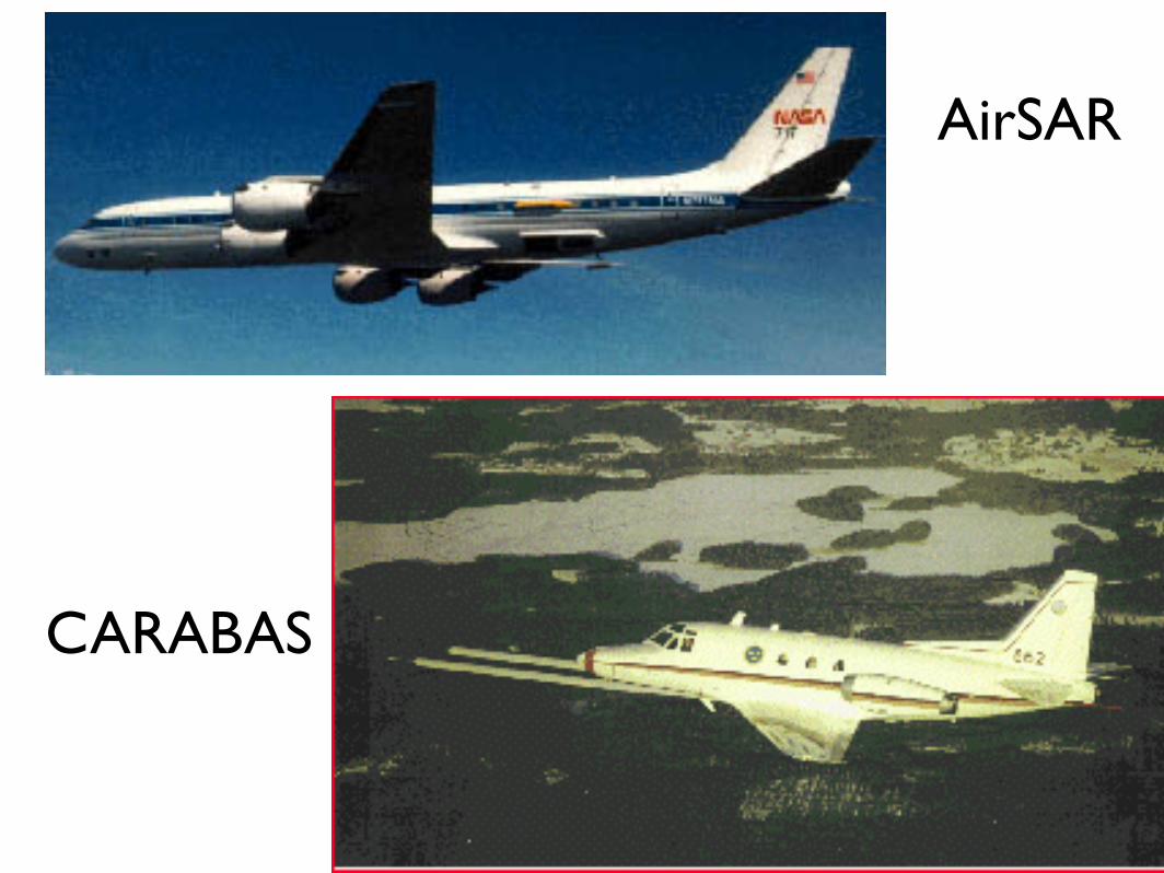
AirSAR
CARABAS

UAVs
Lynx SAR

Applications
• military: early warning, tracking, targeting
• commercial aviation, navigation, collision-avoidance
• land use monitoring, agricultural monitoring, ice patrol,environmental monitoring
• surface topography, crustal change
• speed monitoring (police radar)
• weather radar: storm monitoring, wind shear warning
• search and rescue
• medical microwave tomography
4


Deforestation in Brazil

Ocean waves (texture due to wind)

Oil slicks on the ocean
Sea ice

Ocean internal waves at Gibraltar

SouthernCalifornia
topography


Glacier flowvia SAR
interferometry


Outline
1. introduction, history, frequency bands, dB, real-aperture imaging
2. radar systems: stepped-frequency systems, I/Q demodulation
3. 1D scattering by perfect conductor
4. receiver design, matched filtering
5. ambiguity function & its properties
6. range-doppler (unfocused) imaging
7. introduction to 3D scattering
8. ISAR
9. antenna theory
10. spotlight SAR
11. stripmap SAR
9

Assumed background
• Fourier transform
• delta function
• (!2x ! !2
t )u(t, x) = 0 has solutions of the formu(t, x) = f(t! x) + g(t + x)
• Cauchy-Schwartz inequality (!
fg! " #f##g#)
• f = O(g) means f " (const.)g
• $ · B = 0% B = $&A and $&E = 0% E = !$"
• $&$&E = $($ · E)!$2E
10

Fourier transform
F [F ](t) := f(t) =12!
!e!i!tF (")d" =
!e!2"i#tF (#)d#
inverse transform: F (") =!
ei!tf(t)dt
Properties
1. If g(t) ="
h(t! t")f(t")dt", then G(") = H(")F (").
2. $tf(t) = F [!i"F ](t)
3. %(t) = (2!)!1"
ei!td"
in n dimensions:
F [F ](x) := f(x) =1
(2!)n
!ei!·xF (!)d! F (!) =
!ei!·xf(x)dx
11
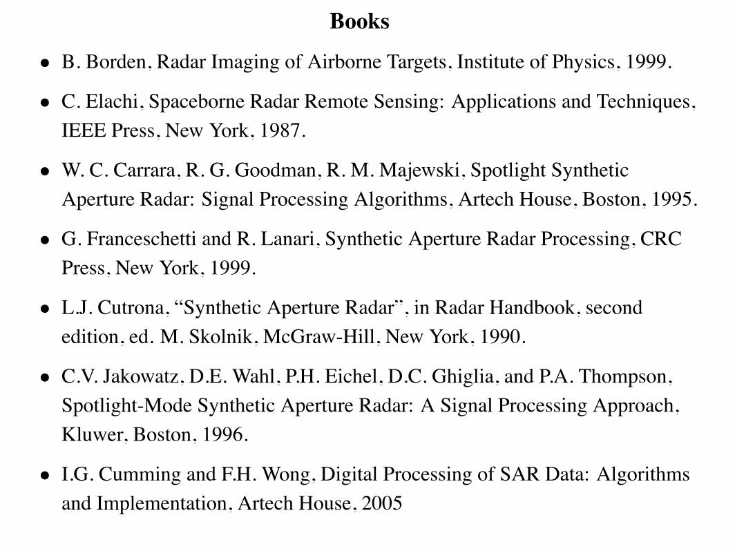
Books
• B. Borden, Radar Imaging of Airborne Targets, Institute of Physics, 1999.
• C. Elachi, Spaceborne Radar Remote Sensing: Applications and Techniques,
IEEE Press, New York, 1987.
• W. C. Carrara, R. G. Goodman, R. M. Majewski, Spotlight Synthetic
Aperture Radar: Signal Processing Algorithms, Artech House, Boston, 1995.
• G. Franceschetti and R. Lanari, Synthetic Aperture Radar Processing, CRC
Press, New York, 1999.
• L.J. Cutrona, “Synthetic Aperture Radar”, in Radar Handbook, second
edition, ed. M. Skolnik, McGraw-Hill, New York, 1990.
• C.V. Jakowatz, D.E. Wahl, P.H. Eichel, D.C. Ghiglia, and P.A. Thompson,
Spotlight-Mode Synthetic Aperture Radar: A Signal Processing Approach,
Kluwer, Boston, 1996.
• I.G. Cumming and F.H. Wong, Digital Processing of SAR Data: Algorithms
and Implementation, Artech House, 2005
46

Maxwell’s equations
!" E = #!tB (1)
!"H = J + !tD (2)
! · D = " ! · B = 0 (3)
E = electric field D = electric displacement
B = magnetic field H = magnetic induction
J = current density " = charge density
Constitutive laws in free space
D = #0E B = µ0H J = 0 " = 0
12

!" (1) + constitutive laws + (2) #
!"!" E! "# $!(! · E)! "# $
0
!"2E
= $!t!"B = $µ0!t!"H! "# $!0"tE
%
!2E $ µ0"0!"#$1/c2
0
!2t E = 0
Fourier transform
%%%%& E(#) ='
ei#tE(t)dt
!2E +#2
c2!"#$
k2
E = 0
13

Atmospheric Attenuation

Radar frequency bands
Band Designation Approximate Frequency Range
HF 3–30 MHz
VHF 30–300 MHz
UHF 300–1000 MHz
L-band 1–2 GHz
S-band 2–4 GHz
C-band 4–8 GHz
X-band 8–12 GHz
Ku-band 12–18 GHz
K-band 18–27 GHz
Ka-band 27–40 GHz
mm-wave 40–300 GHz
15

Decibels
log10
!power inpower out
"= Bel too small
instead use:
decibel dB = 10 log10power inpower out = 10 log10
V 2in
V 2out
= 20 log10Vin
Vout
!power " (voltage)2
dB Power ratio
0 dB 1
10 dB 10
20 dB 100
30 dB 1000
16

Outline
1. introduction, history, frequency bands, dB, real-aperture imaging
2. radar systems: stepped-frequency systems, I/Q demodulation
3. 1D scattering by perfect conductor
4. receiver design, matched filtering
5. ambiguity function & its properties
6. range-doppler (unfocused) imaging
7. introduction to 3D scattering
8. ISAR
9. antenna theory
10. spotlight SAR
11. stripmap SAR
9

Radar systems
1. Stepped-frequency radars (laboratory systems)
transmit receive measure
cos(!1t)! "# $Re(e!i!1t)
RR(!1) cos(!1t) + RI(!1) sin(!1t)! "# $Re[R(!1)e!i!1t]
R(!1)
Re(e!i!2t) R(!2)e!i!2t R(!2)...
......
Re(e!i!N t) R(!N )e!i!N t R(!N )
From the Rs, can synthesize response to any waveform
sin(t) =%
an(!n)e!i!nt !& !N
!1
a(!)e!i!td!
Response would be
srec(t) =%
an(!n)R(!n)e!i!nt !& !N
!1
a(!)R(!)e!i!td!
17


waveform
generator
transmitter
(amplifier)
I/Q
demodulator
correlation
receiver
circulator
antenna
low-noise
amplifier (LNA)
⊗s(t)
cos ! t c
p(t) = s(t)cos ! t c
p (t) = a(t) cos[ ! t +" (t)]crec
2. Pulsed radar systems

I/Q Demodulation
in-phase (I) channel:
prec(t) cos(!ct) = a(t) cos("(t) + !ct) cos(!ct)
= a(t) 12
!
"#cos("(t) + 2!ct)$ %& 'filter out
+cos "(t)
(
)*
quadrature (Q) channel (90! out of phase):prec(t) sin(!ct) = a(t) cos("(t) + !ct) sin(!ct)
= a(t) 12
!
"#! sin("(t) + 2!ct)$ %& 'filter out
+sin"(t)
(
)*
I and Q channels together give the analytic signal
srec(t) = a(t)ei!(t)
(approximately analytic in upper half-plane, when a(t) is slowly varying,i.e., in narrowband case)
19

Filters
H(!) transfer function
f(t) F!" F (!)"
!"#" F (!)H(!) F
!1
!" (h # f)(t)
F!1 [H(!)(Ff)(!)] (t) =12"
$e!i!tH(!)
$ei!t"f(t")dt"d!
=12"
$ %$e!i!(t!t")H(!)d!
&
' () *h(t!t")
f(t")dt"
Example: Low-pass filter. Take H(!) =+
1 |!| < !1
0 otherwise
$ h(t) = !1"
sin !1t!1t = !1
" sinc !1t
20

Outline
1. introduction, history, frequency bands, dB, real-aperture imaging
2. radar systems: stepped-frequency systems, I/Q demodulation
3. 1D scattering by perfect conductor
4. receiver design, matched filtering
5. ambiguity function & its properties
6. range-doppler (unfocused) imaging
7. introduction to 3D scattering
8. ISAR
9. antenna theory
10. spotlight SAR
11. stripmap SAR
9

1D Scattering by a fixed perfect conductor at range R
waveform generator! sinc(t)transmitter output:
sinc(t) cos(!ct) = Re!sinc(t)e!i!ct
":= f(t)
transmitted electromagnetic wave: (1D model)
Ein(r, t) = einf(t" x/c) where x = e · r
Ein is a right-going solution of
"2xEin " 1
c2"2
t Ein = 0
Write total field as Etot = Ein + Esc (think f(t" x/c) + g(t + x/c))Etot satisfies
"2xEtot " 1
c2"2
t Etot = 0
Etot
####x=R
= 0 # conducting B.C.
22

!
!2xEsc " 1
c2!2
t Esc = 0
Esc
!!!!x=R
= "Ein
!!!!x=R
expect Esc(r, t) = escg(t + x/c) (left-going solution of wave equation)
B.C.! escg(t + R/c" #$ %w
) = "einf(t"R/c) ! esc = "ein
t = w "R/c ! g(w) = f(w " 2R/c)
received field at r = 0:Esc(0, t) = "einf(t" 2R/c)
transmit f(t), receive prec(t) = f(t" 2R/c) (fixed target)
23

1D Scattering by a moving conductor at range R(t)
g(t + R(t)/c! "# $w
) = f(t!R(t)/c)
solve w = t + R(t)/c for t (via Implicit Function Theorem)" t = !(w)
for pulsed systems: use Taylor series expansion R(t) = R + vt + · · ·
w = t +
R(t)# $! "(R + vt) /c # t =
w !R/c
1 + v/c:= !(w)
g(w) = f(t! (R + vt)/c)%%t=!(w)
= f
&
''(
)1! v/c
1 + v/c
*
! "# $"
(w !R/c)!R/c
+
,,-
$Doppler scale factor
24
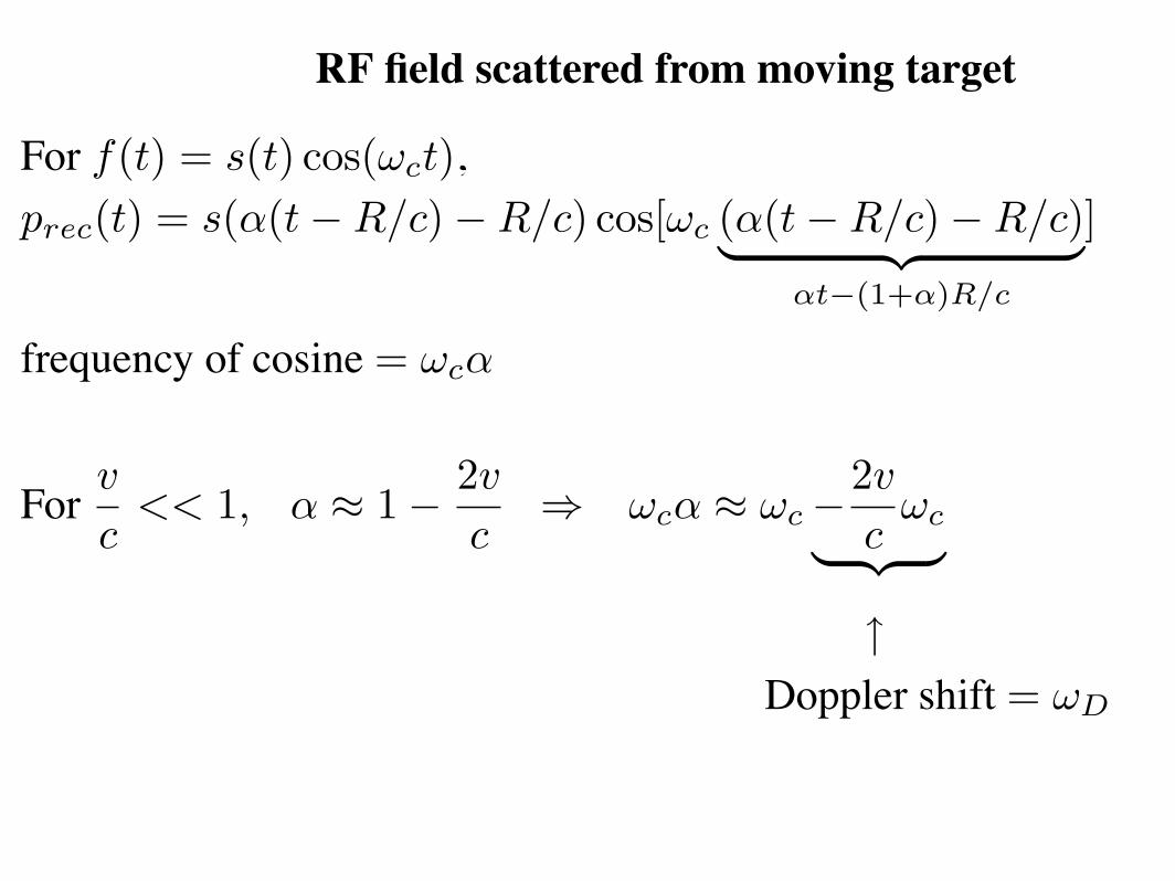
RF field scattered from moving target
For f(t) = s(t) cos(!ct),prec(t) = s("(t!R/c)!R/c) cos[!c ("(t!R/c)!R/c)! "# $
!t!(1+!)R/c
]
frequency of cosine = !c"
Forv
c<< 1, " " 1! 2v
c# !c" " !c!
2v
c!c
! "# $
$Doppler shift = !D
24

I/Q demodulation of signal from moving scatterer
prec(t) cos(!ct) = s("(t!R/c)!R/c) cos[!c("t! (1 + ")R/c)] cos(!ct)
= s("(t!R/c)!R/c)12
! filter out" #$ %cos[sum] + cos [!c("t! (1 + ")R/c)! !ct]
&
I(t) = s("(t!R/c)!R/c) cos !c [("! 1)t! (1 + ")R/c)]Q(t) = s("(t!R/c)!R/c) sin!c [("! 1)t! (1 + ")R/c)]
srec(t) = s("(t!R/c)!R/c)ei!c[("!1)t!(1+")R/c)]
For vc << 1 and s slowly varying:
srec(t) " s(t! 2R/c)ei!D(t!R/c)e!2i!cR/c
25

Outline
1. introduction, history, frequency bands, dB, real-aperture imaging
2. radar systems: stepped-frequency systems, I/Q demodulation
3. 1D scattering by perfect conductor
4. receiver design, matched filtering
5. ambiguity function & its properties
6. range-doppler (unfocused) imaging
7. introduction to 3D scattering
8. ISAR
9. antenna theory
10. spotlight SAR
11. stripmap SAR
9

waveform
generator
transmitter
(amplifier)
I/Q
demodulator
correlation
receiver
circulator
antenna
low-noise
amplifier (LNA)
⊗s(t)
cos ! t c
p(t) = s(t)cos ! t c
p (t) = a(t) cos[ ! t +" (t)]crec
2. Pulsed radar systems

Receiver design
For good range resolution, want a short pulse
But a short pulse has little energy! hard to detect signal in noise
energy density " 1R4 !
signal is swamped by thermal noise in the receiver!
target can’t even be detected, much less imaged
Brilliant solution:
Use (long) coded pulses and mathematical processing
#matched filter or correlation receiver
pulse compression
27

Matched filter: sketch of derivation
receiver input: r(t) = !s(t! ") + n(t) ( = demodulator output)
" " # want to find "
aei!/R4 2R/c noise, assumed white, zero mean
power spectral density N
Apply filter #(t) = (h $ r)(t) =!
h(t! t!)r(t!)dt! = #s(t) + #n(t)Choose h so that |#s(")/#n(")| is as large as possible.
SNR = maxh
|#s(")|2
E|#n(")|2 = maxh
!2""! h(" ! t!)s(t! ! ")dt!
""2
N!
|h(t)|2dt
= maxh
!2""! h(t!)s(!t!)dt!
""2
N!
|h(t)|2dt
Cauchy-Schwartz inequality% h(t) = s"(!t)
#(t) =!
s"(t! ! t)r(t!)dt! =!
s"(t!!)r(t + t!!)dt!! correlation
29
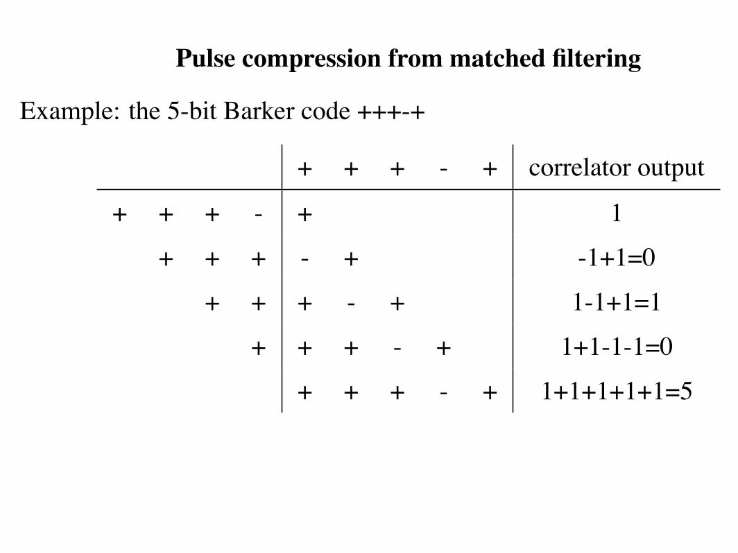
Pulse compression from matched filtering
Example: the 5-bit Barker code +++-+
+ + + - + correlator output
+ + + - + 1
+ + + - + -1+1=0
+ + + - + 1-1+1=1
+ + + - + 1+1-1-1=0
+ + + - + 1+1+1+1+1=5
30

Multiple fixed targets
Two fixed targets: r(t) = !1s(t! "1) + !2s(t! "2) + n(t)
Distribution of fixed targets: r(t) =!
!(" !)s(t! " !)d" ! + n(t)
Apply matched filter:
#(t) ="
s"(t! ! t)r(t!)dt!
="
s"(t! ! t)"
!(" !)s(t! ! " !)d" !dt! + noise
=" "
s"(t! ! t)s(t! ! " !)dt!
# $% &!(" !#t)
!(" !)d" ! + noise
$(t) =!
s"(t!! + t)s(t!!)dt!! = point spread function for
1D “imaging system”
30

31
High Range-Resolution (HRR) Imaging

Chirp = Linearly Frequency Modulated (LFM) waveform
s(t) = ei!(t)rect(t/tp) where d!dt (t) = instantaneous frequency
rect(t) =!
1 !1/2 < t < 1/20 otherwise
d!dt (t) = at " !(t) = at2
" s(t) = eiat2rect(t/tp)
gives rise to a point spread function
"(t) = (1! |t|)sinc(at(1! |t|))
where sinc x = (1/x) sinx.
(see p. 170 in Rihaczek Principles of High Resolution Radar
or work out yourself)
32
Chirp
! " # $ % & ' ( ) * "!!"
!!+)
!!+'
!!+%
!!+#
!
!+#
!+%
!+'
!+)
"
an upchirp Fourier transform of chirp
33

Matched filter for single moving target
receiver input = demodulator output = r(t) = s(t! !)ei!D(t!") + n(t)want to find ! and "D.
use a filter bank = set of filters that depend on a parameter #:
$(t, #) =!
h#(t! t")r(t")dt"
to maximize SNR, choose h#(t) = s#(!t)ei2$#t
34

Matched filter for distribution of moving targets
demodulator output = r(t) =! !
!(" !, #!)s(t! " !)e2!i"!(t"# !)d" !d#!
output of filter bank is
$(t, #) ="
s#(t! ! t)e2!i"(t"t!)r(t!)dt!
="
s#(t! ! t)e2!i"(t"t!)s(t! ! " !)e2!i"!(t!"# !)dt!!(" !, #!)d" !d#!
=" "
%(" ! ! t, #! ! #)e2!i"(t"# !)!(" !, #!)d" !d#!
where
%(", #) =!
s#(t!! + ")s(t!!)e2!i"t!!dt!!
(narrowband) radar ambiguity function
point spread function for imaging system
Typically one considers only the magnitude of the ambiguity function.
35

Outline
1. introduction, history, frequency bands, dB, real-aperture imaging
2. radar systems: stepped-frequency systems, I/Q demodulation
3. 1D scattering by perfect conductor
4. receiver design, matched filtering
5. ambiguity function & its properties
6. range-doppler (unfocused) imaging
7. introduction to 3D scattering
8. ISAR
9. antenna theory
10. spotlight SAR
11. stripmap SAR
9
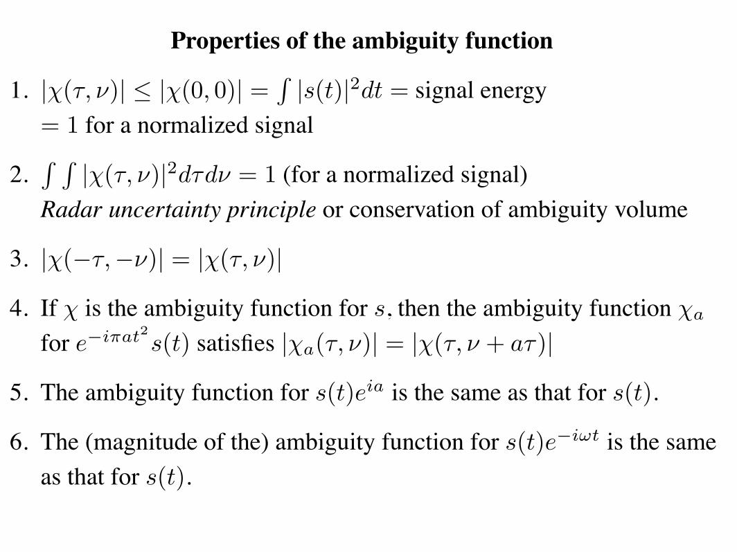
Properties of the ambiguity function
1. |!(", #)| ! |!(0, 0)| =!
|s(t)|2dt = signal energy
= 1 for a normalized signal
2.! !
|!(", #)|2d"d# = 1 (for a normalized signal)Radar uncertainty principle or conservation of ambiguity volume
3. |!("","#)| = |!(", #)|
4. If ! is the ambiguity function for s, then the ambiguity function !a
for e!i!at2s(t) satisfies |!a(", #)| = |!(", # + a")|
5. The ambiguity function for s(t)eia is the same as that for s(t).
6. The (magnitude of the) ambiguity function for s(t)e!i"t is the same
as that for s(t).
37

Resolution and cuts through the ambiguity function
Doppler (frequency) resolution:
|!(0, ")| =!!!!"
|s(t)|2e2!i"tdt
!!!!
! Frequency (Doppler) resolution is determined by amplitude.
For good Doppler resolution, want |s(t)| " 1.
Range resolution:
|!(#, 0)| =!!!!"
|S(2$")|2e2!i"#d"
!!!!
where S(%) =#
e!i$ts(t)dt.
! Range resolution (for a fixed target) is determined by bandwidth.
38

Example: Range resolution with a CW pulse
baseband signal is s(t) = rect(t/tp) tp = time duration of pulse
ambiguity function is
|!(", #)| =! "
1! |! |tp
# $$$sinc%$#tp
"1! |! |
tp
#&$$$ for |" | < tp
0 otherwise
Range resolution is obtained from
|!(", 0)| =! "
1! |! |tp
#for |" | < tp
0 otherwise
whose first null is at %"pn = tp.
39

N. Levanon, Radar Principles,
Wiley 1988
ambiguityfunction
for CW pulse
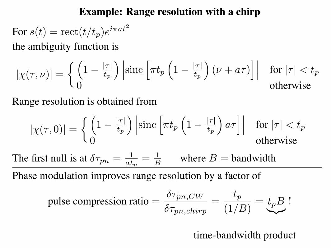
Example: Range resolution with a chirp
For s(t) = rect(t/tp)ei!at2
the ambiguity function is
|!(", #)| =! "
1! |" |tp
# $$$sinc%$tp
"1! |" |
tp
#(# + a")
&$$$ for |" | < tp
0 otherwise
Range resolution is obtained from
|!(", 0)| =! "
1! |" |tp
# $$$sinc%$tp
"1! |" |
tp
#a"
&$$$ for |" | < tp
0 otherwise
The first null is at %"pn = 1atp
= 1B where B = bandwidth
Phase modulation improves range resolution by a factor of
pulse compression ratio =%"pn,CW
%"pn,chirp=
tp(1/B)
= tpB'()*!
time-bandwidth product
40
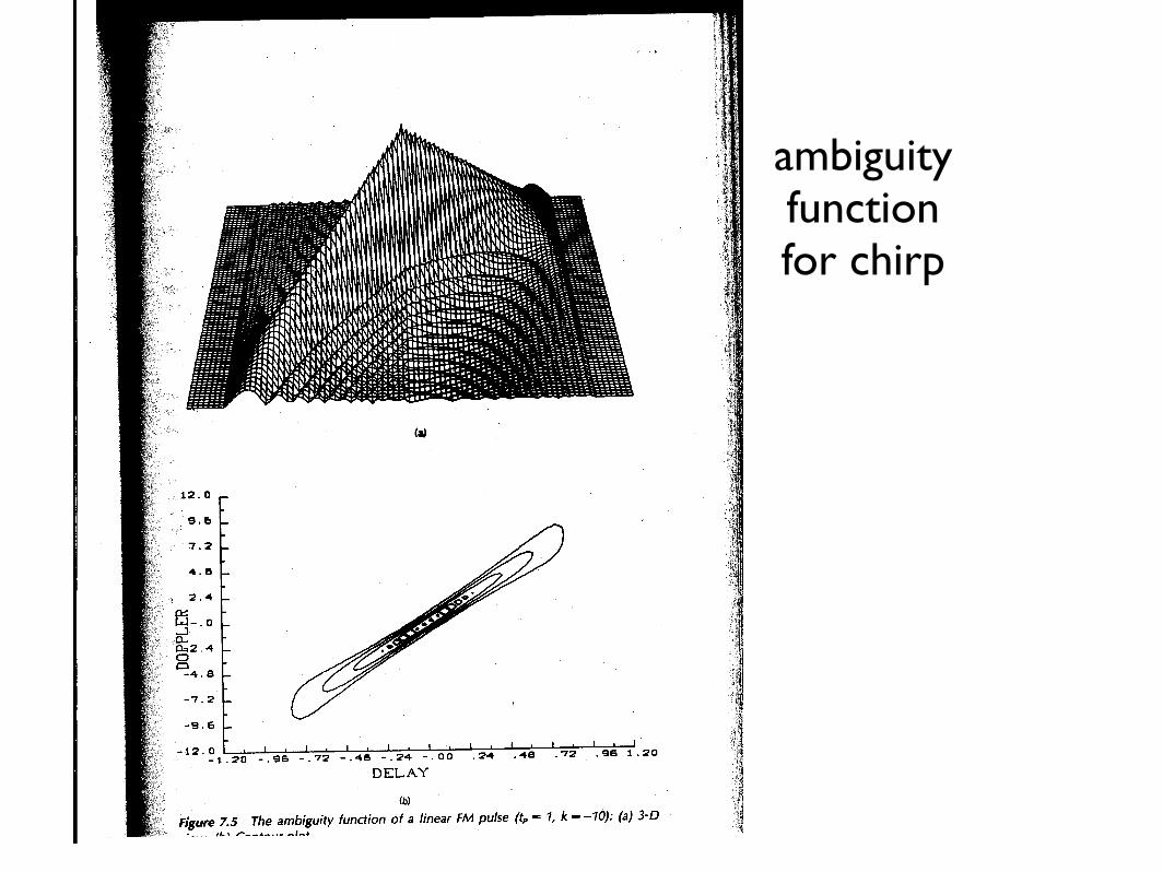
ambiguityfunctionfor chirp

A train of high-range-resolution (HRR) pulses
Doppler shift can be found by change in phase of successive returns
Suppose target travels as R(t) = R0 + vt; write Rn = R(nT )
1. transmit pn(t) = s(t)e!i!ct
receive rn(t) = pn(t! 2Rn/c)ei!D(t!2Rn/c)
2. demodulate: sn(t) = s(t! 2Rn/c)ei!D(t!Rn/c)e!2i!cRn/c
3. correlate: !n(") =!
s"(t# ! ")sn(t#)dt# =!s"(t# ! ")s(t# ! 2Rn/c)ei!D(t!!Rn/c)e!2i!cRn/cdt#
4. at peak, " = 2Rn/c:
!n(2Rn/c) =!
|s(t# ! 2Rn/c)|2ei!D(t!!Rn/c)dt#" #$ %
"(0,!D)
e!2i!cRn/c
5. phase difference between successive pulses:
2#c[R0 + v(n + 1)T ]/c! 2#c[R0 + vnT ]/c = 2#cv/c = !#D
6. note blind speeds when 2#cv/c = 2$(integer)
42

ambiguity function for
a train of pulses
pulse repetitionfrequency gives
rise to delayambiguities

Outline
1. introduction, history, frequency bands, dB, real-aperture imaging
2. radar systems: stepped-frequency systems, I/Q demodulation
3. 1D scattering by perfect conductor
4. receiver design, matched filtering
5. ambiguity function & its properties
6. range-doppler (unfocused) imaging
7. introduction to 3D scattering
8. ISAR
9. antenna theory
10. spotlight SAR
11. stripmap SAR
9
!
!
x
v
(x,y)
r
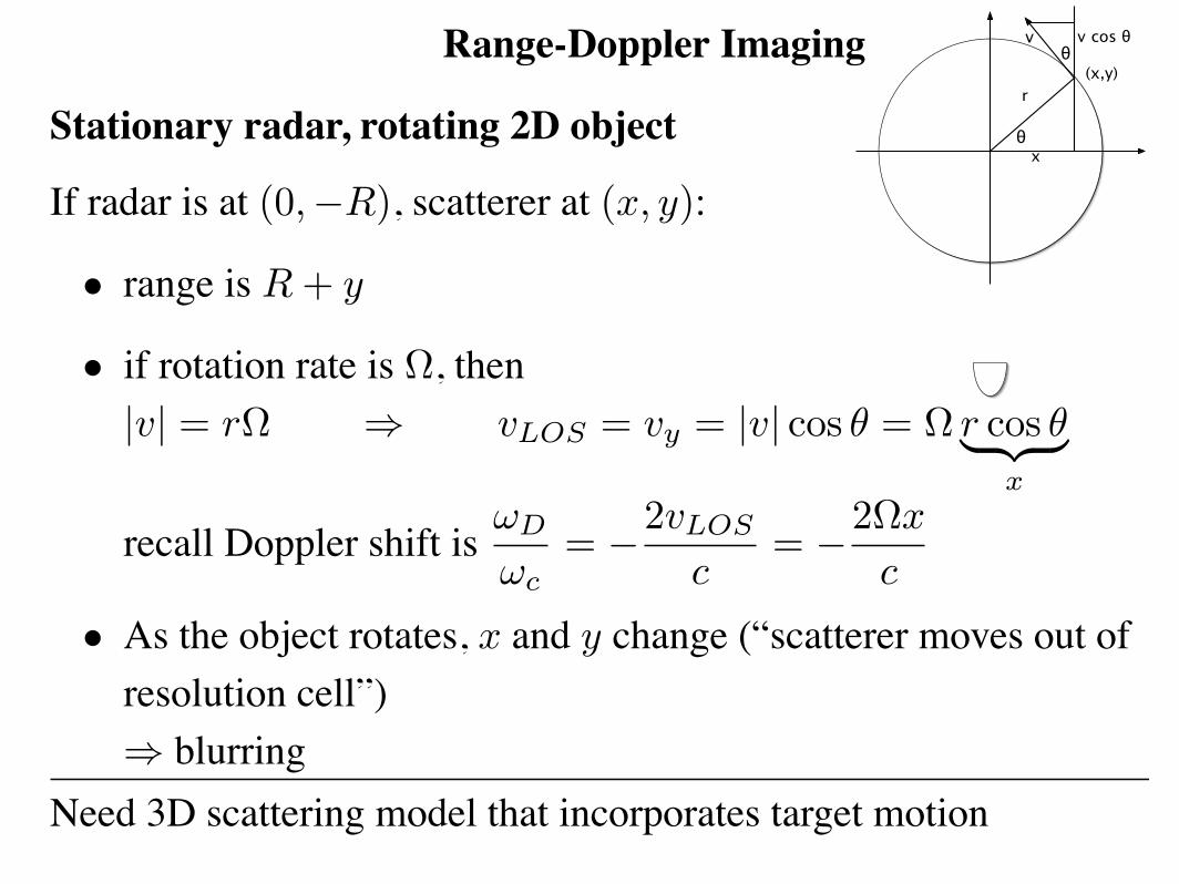
v cos ! Range-Doppler Imaging
Stationary radar, rotating 2D object
If radar is at (0,!R), scatterer at (x, y):
• range is R + y
• if rotation rate is !, then|v| = r! " vLOS = vy = |v| cos ! = ! r cos !! "# $
x
recall Doppler shift is"D
"c= !2vLOS
c= !2!x
c
• As the object rotates, x and y change (“scatterer moves out of
resolution cell”)
" blurring
Need 3D scattering model that incorporates target motion
42

Moving radar imaging a stationary planar scene
• delay! range! scatterer lies on a constant-range sphere
! scatterer on plane lies on a constant-range circle
• Doppler shift! line-of-sight relative velocity
! scatterer lies on the iso-Doppler cone vLOS = R · v = const
! scatterer on plane lies on iso-Doppler hyperbola
• does not account for change in radar position as measurements are
taken (“scatterers migrate through resolution cell”)
! get an unfocused image
Need a 3D scattering model that incorporates changes in sensor position
43

