RADIANCE: a simulation tool for daylighting systems

Dr. R. Compagnon

University of Applied Sciences of Western Switzerland (HES-SO) Ecole d'ingenieurs et d'architectes de Fribourg (EIA-FR)

80 Bd Perolles, 1705 Fribourg Switzerland Tel: +41 26 429 6666 Fax: +41 26 429 6600

(Revised version for UNIX/LINUX; December 2001)

This document serves as course notes. It is intended to complement the RADIANCE original documentation giving more details in some essential areas. Technical terms used within this document come mainly from the lighting domain [CIE87] or the computer graphics domain [Jem92]; the remaining terms are part of the specific jargon employed in the RADIANCE original documentation. This character type refers either to a command (a program name) or the content of a file. Adjustable parameters appear in italic. Table of contents

Introduction................................................................................2 Physical basis............................................................................3 General structure of the software ..............................................5 Structure of a "scene" file ..........................................................6 Model of a sky ...........................................................................7 Interactive visualisation using rview ........................................8 The "exposure" of a RADIANCE picture ....................................9 Rendering a picture using rpict ............................................10 Special projections using rtrace ...........................................11 Picture processing ...................................................................12 Model of a room daylit by an anidolic light-shelf ......................14 How ray tracing works within RADIANCE................................15 Illuminance calculations...........................................................21 False colour pictures................................................................22 Assessing discomfort glare......................................................23 Simulations with sunny skies ...................................................25 A few words on textures and patterns .....................................27 Automation of the rendering process using rad ......................28 RADIANCE distribution and user support ................................29 References ..............................................................................30 Acknowledgements..................................................................32 Appendices..............................................................................33

2

Introduction RADIANCE development started in 1984 at the Lawrence Berkeley Laboratory (Berkeley, USA). At the same time, the "radiosity" method was first applied in the computer graphics domain. The "ray tracing" method already used since the 1970s was considered to be incapable of computing interreflections in a reasonable amount of time (note that this idea still perpetuates in some recent publications). The most original part of RADIANCE lies within its interreflection calculation algorithm that uses a backward ray tracing method [War88a&b] [War92a]. As far as we know this is one of the rare (or even the unique) implementations of a purely ray tracing interreflection algorithm in a realistic rendering program; almost all other similar programs are based on radiosity algorithms. In 1990 the Laboratoire d’Energie Solaire et de Physique du Bâtiment (LESO-PB in Lausanne, Switzerland) initiated a project on daylighting simulation tools [Sca94]. Greg Ward, the principal author of RADIANCE, joined that project for 9 months during which he greatly extended the capabilities of the software especially for daylighting simulation purposes. In parallel, RADIANCE has been included into the ADELINE software developed within an IEA task. Since then, RADIANCE has been available in two versions: the original one as free software for UNIX workstations and a slightly limited MS-DOS version included within ADELINE. The latter is distributed by the research teams that have contributed to ADELINE. More recently a new version named “Desktop RADIANCE” running on Windows and interfaced with AutoCAD has appeared and is distributed by the LBL. This course is based on the original UNIX Radiance version. RADIANCE is currently a mature ray tracing software package that enables accurate and physically valid lighting and daylighting simulations [War90] [War94b] [Lar98]. It is well established in the research community and has already been used for many projects [War89] [Com92-94] [Pau92] [Fro93] [Lom93] [Nov93] [War94c] [Cla96] [Moe96]. Some validation studies have also been carried out on RADIANCE (see for instance references [Gry88-89] [Com94] and [Mar97]). Due to to the great flexibility of RADIANCE (almost all calculation procedures can be specifically controlled by the users through appropriate parameters), any validation study reflects more the skills of the user who performed it than just the accuracy of the internal algorithms! However, there are many appropriate ways of using RADIANCE and the material presented in this document should not be considered as the unique or best practice for accurate simulation of daylighting systems. Remarks: A ray tracing bibliography is maintained on the Internet at: http://liinwww.ira.uka.de/bibliography/Graphics/ray.html A large bibliography on radiosity as well as other very interesting documents regarding this technique are also available on the Internet at: http://www.ledalite.com/resources/white/index.html

3

Physical basis RADIANCE is based on the backward ray tracing algorithm. This means that light rays are traced in the opposite direction to that which they naturally follow. The process starts from the eye (the viewpoint) and then traces the rays up to the light sources taking into account all physical interactions (reflection, refraction) with the surfaces of the objects composing the scene. Polarisation of light rays is not taken into account. RADIANCE uses a geometrical description of the "scene" based on the boundaries of objects (i.e. their external surfaces). The volumes enclosed by these surfaces are always empty. Surfaces have definite orientation (i.e. a normal vector is attached to each surface). The objects composing the scene are described using a Cartesian co-ordinate system (X,Y,Z). Originally the X axis is directed towards the East, the Y axis towards the North and the Z axis towards the zenith. It is usually much more convenient to align the principal planes of the scene (e.g. the walls of a rectangular room) along the X,Y,Z axes and then to rotate the sky description around the Z axis in order to correctly orient the scene (this will be explained later). Co-ordinates can be given in any unit of length. Of course when a single scene is formed by more than one scene file, these must use same unit of length. Each single ray "carries" a certain amount of radiance (hence the name of the software) expressed in [W/m2sr]. The radiance is divided into three "channels" corresponding to the red, green and blue primary colours (abbreviated as r,g,b). The total radiance R is calculated as a weighted sum of the radiances Rr, Rg and Rb carried by the three channels: R = 0.265.Rr + 0.670.Rg + 0.065.Rb [W/m2sr] (note that: 0.265+0.670+0.065 = 1) The transformation from radiance R (radiometric unit) to luminance L (photometric unit) is given by: L = 179.R = 47.4.Rr + 119.9.Rg + 11.7.Rb [cd/m2] This method of handling colours relates to a perceptual model which is unable to fully account for spectrally dependent properties. Compared to programs where the spectral distribution of the light is modelled using many channels covering narrow wavelength bands, RADIANCE is less precise and is unable to model all possible colours. This disadvantage is far outweighted by the fact that colour data for materials are much more frequently available as colorimetric values (e.g. CIE XYZ tristimulus system). than as detailed spectral curves! In addition, for our type of application spectral effects are rather limited since colours commonly used in buildings are not very saturated (i.e. their spectral reflection curves are smooth).

4

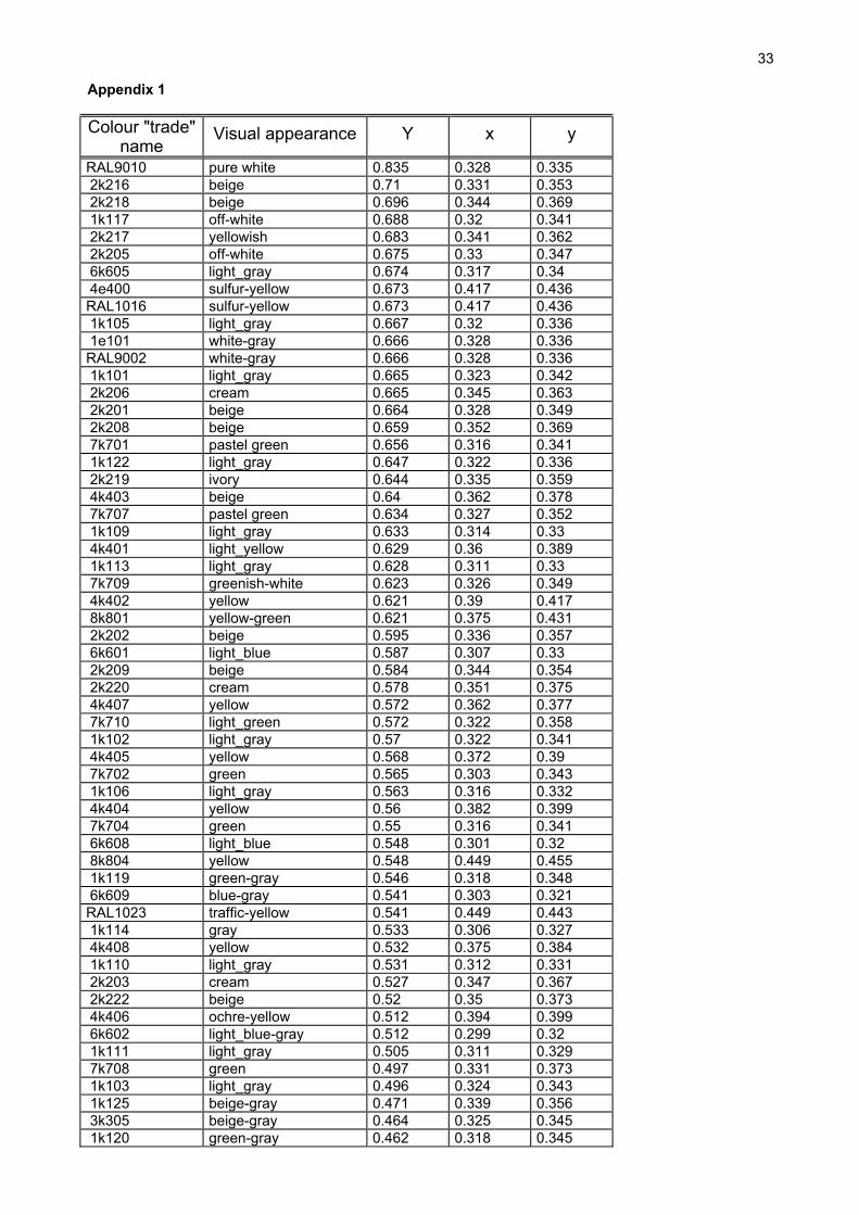
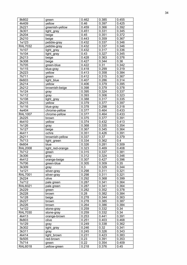
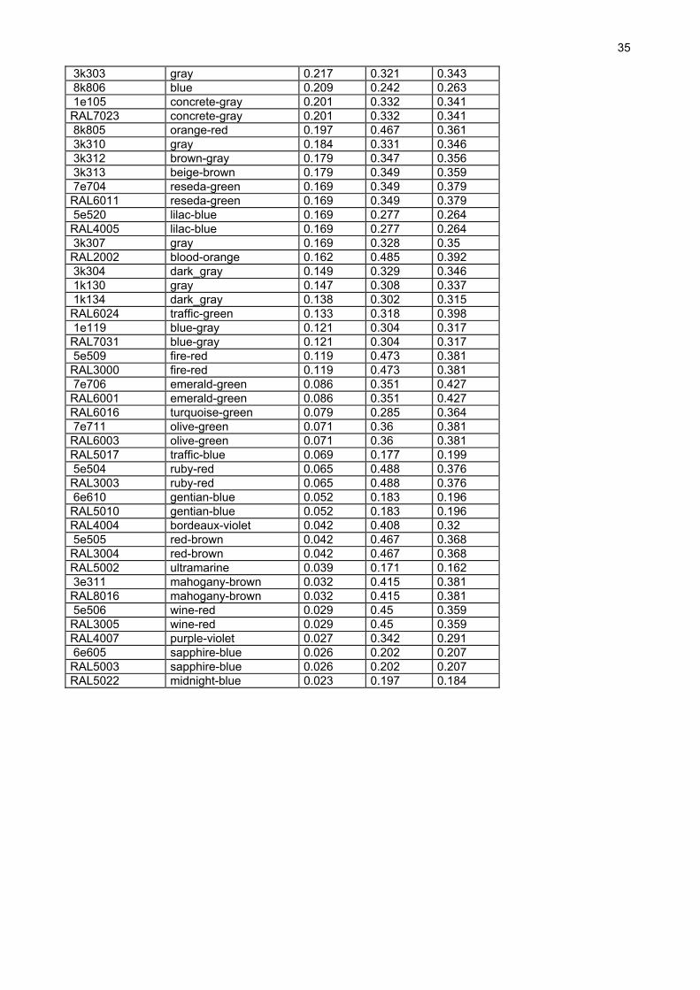
From the Y,x,y values the reflectances or transmittances C of the corresponding materials are divided into the three red, green and blue channels as follows (see file: rgb.cal):

Cr = 2.565.X -1.167.Y -0.398.Z Cg = -1.022.X +1.978.Y +0.044.Z Cb = 0.075.X -0.252.Y +1.177.Z where: X = x.Y/y Z = (1-x-y).Y/y

Exercise: Start the calc program by typing the command: calc rgb.cal and use it to calculate the reflectances Cr Cg and Cb of some paints whose Y,x,y values are listed in Appendix 1. Remarks: The principles of tristimulus colorimetry and the transformations from Y,x,y to Cr, Cg and Cb values are presented in a tutorial fashion in [Mey86]. An annotated bibliography of relevant literature is also provided. See also the "Frequently Asked Questions about color" document available on the Internet from the page: http://Home.InfoRamp.Net/~poynton/ "Photometry and Radiometry; a Tour Guide for Computer Graphics Enthusiasts" provides a good tutorial on this subject. It is available on the Internet from the page: http://www.ledalite.com/resources/white/index.html

5

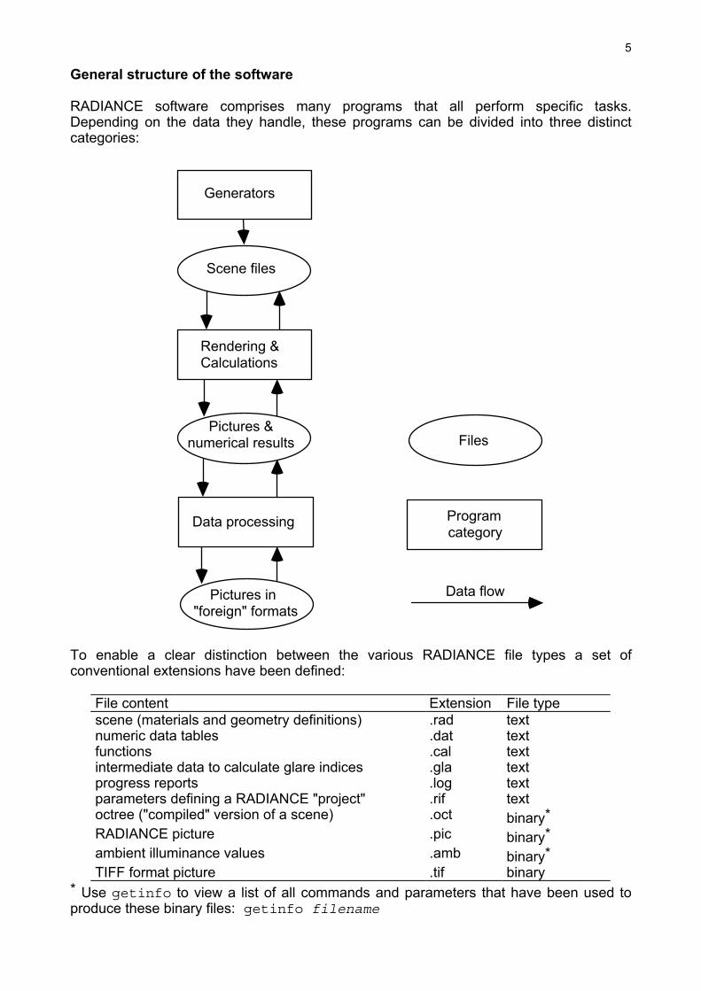
General structure of the software RADIANCE software comprises many programs that all perform specific tasks. Depending on the data they handle, these programs can be divided into three distinct categories:

Scene files

Generators

Rendering & Calculations

Pictures & numerical results

Data processing

Pictures in "foreign" formats

Program category

Files

Data flow

To enable a clear distinction between the various RADIANCE file types a set of conventional extensions have been defined:

File content Extension File type scene (materials and geometry definitions) .rad text numeric data tables .dat text functions .cal text intermediate data to calculate glare indices .gla text progress reports .log text parameters defining a RADIANCE "project" .rif text octree ("compiled" version of a scene) .oct binary* RADIANCE picture .pic binary* ambient illuminance values .amb binary* TIFF format picture .tif binary

* Use getinfo to view a list of all commands and parameters that have been used to produce these binary files: getinfo filename

6

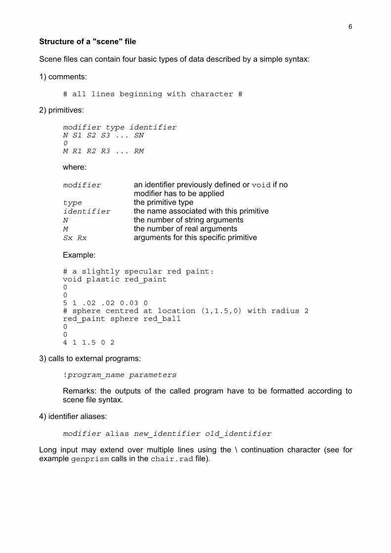
Structure of a "scene" file Scene files can contain four basic types of data described by a simple syntax: 1) comments:

# all lines beginning with character #

2) primitives: modifier type identifier N S1 S2 S3 ... SN 0 M R1 R2 R3 ... RM where: modifier an identifier previously defined or void if no modifier has to be applied type the primitive type identifier the name associated with this primitive N the number of string arguments M the number of real arguments Sx Rx arguments for this specific primitive Example: # a slightly specular red paint: void plastic red_paint 0 0 5 1 .02 .02 0.03 0 # sphere centred at location (1,1.5,0) with radius 2 red_paint sphere red_ball 0 0 4 1 1.5 0 2 3) calls to external programs: !program_name parameters Remarks: the outputs of the called program have to be formatted according to

scene file syntax. 4) identifier aliases: modifier alias new_identifier old_identifier Long input may extend over multiple lines using the \ continuation character (see for example genprism calls in the chair.rad file).

7

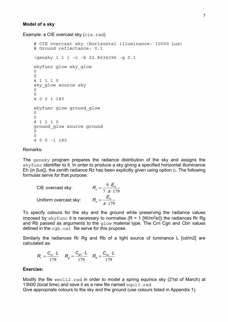
Model of a sky Example: a CIE overcast sky (cie.rad)

# CIE overcast sky (Horizontal illuminance: 10000 Lux) # Ground reflectance: 0.1 !gensky 1 1 1 -c -b 22.8634396 -g 0.1 skyfunc glow sky_glow 0 0 4 1 1 1 0 sky_glow source sky 0 0 4 0 0 1 180 skyfunc glow ground_glow 0 0 4 1 1 1 0 ground_glow source ground 0 0 4 0 0 -1 180

Remarks: The gensky program prepares the radiance distribution of the sky and assigns the skyfunc identifier to it. In order to produce a sky giving a specified horizontal illuminance Eh (in [lux]), the zenith radiance Rz has been explicitly given using option b. The following formulas serve for that purpose:

CIE overcast sky: R Ez

h= ⋅⋅ ⋅9

7 179π

Uniform overcast sky: R Ez

h=⋅π 179

To specify colours for the sky and the ground while preserving the radiance values imposed by skyfunc it is necessary to normalise (R = 1 [W/m2sr]) the radiances Rr Rg and Rb passed as arguments to the glow material type. The Crn Cgn and Cbn values defined in the rgb.cal file serve for this prupose. Similarly the radiances Rr Rg and Rb of a light source of luminance L [cd/m2] are calculated as:

R C Lr

rn= ⋅179

RC L

ggn=

⋅179

R C Lb

bn= ⋅179

Exercise: Modify the file wsol12.rad in order to model a spring equinox sky (21st of March) at 13h00 (local time) and save it as a new file named equ13.rad Give appropriate colours to the sky and the ground (use colours listed in Appendix 1).

8

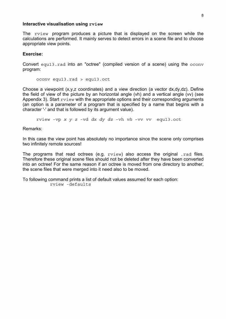
Interactive visualisation using rview The rview program produces a picture that is displayed on the screen while the calculations are performed. It mainly serves to detect errors in a scene file and to choose appropriate view points. Exercise: Convert equ13.rad into an "octree" (compiled version of a scene) using the oconv program: oconv equ13.rad > equ13.oct Choose a viewpoint (x,y,z coordinates) and a view direction (a vector dx,dy,dz). Define the field of view of the picture by an horizontal angle (vh) and a vertical angle (vv) (see Appendix 3). Start rview with the appropriate options and their corresponding arguments (an option is a parameter of a program that is specified by a name that begins with a character '-' and that is followed by its argument value).

rview -vp x y z -vd dx dy dz -vh vh -vv vv equ13.oct

Remarks: In this case the view point has absolutely no importance since the scene only comprises two infinitely remote sources! The programs that read octrees (e.g. rview) also access the original .rad files. Therefore these original scene files should not be deleted after they have been converted into an octree! For the same reason if an octree is moved from one directory to another, the scene files that were merged into it need also to be moved. To following command prints a list of default values assumed for each option:

rview -defaults

9

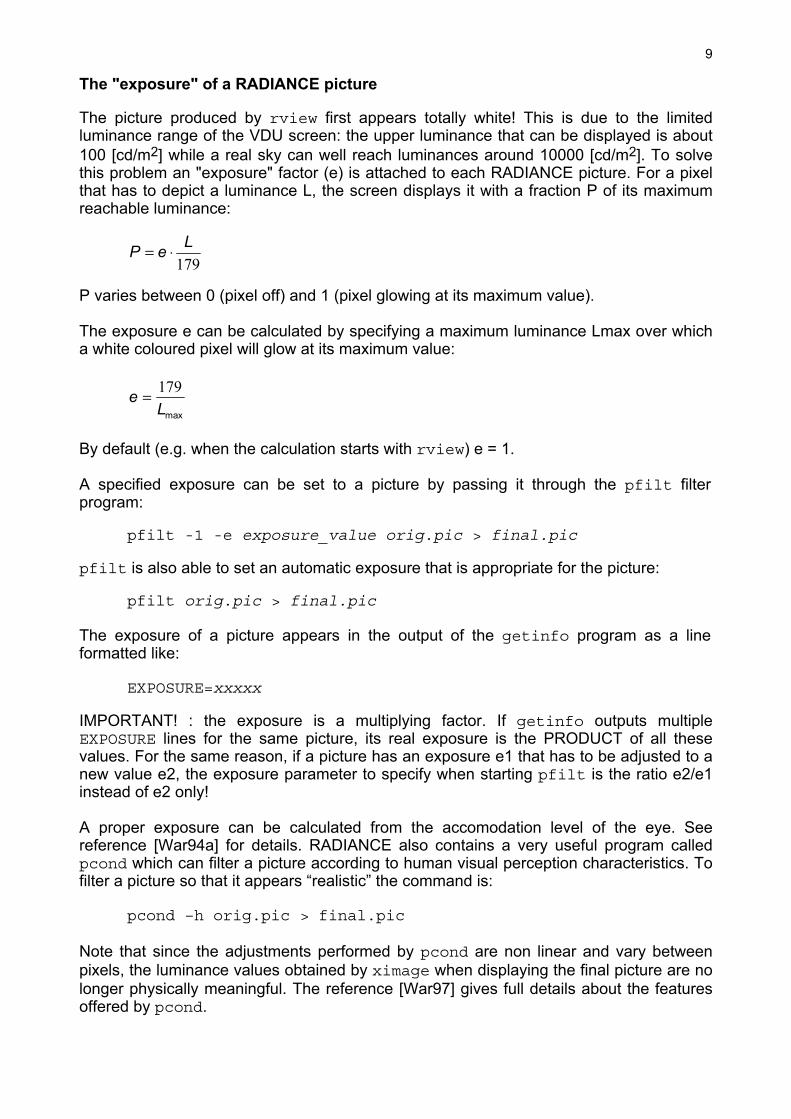
The "exposure" of a RADIANCE picture The picture produced by rview first appears totally white! This is due to the limited luminance range of the VDU screen: the upper luminance that can be displayed is about 100 [cd/m2] while a real sky can well reach luminances around 10000 [cd/m2]. To solve this problem an "exposure" factor (e) is attached to each RADIANCE picture. For a pixel that has to depict a luminance L, the screen displays it with a fraction P of its maximum reachable luminance:

P e L= ⋅179

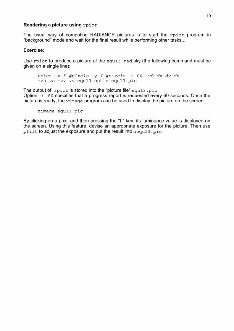
P varies between 0 (pixel off) and 1 (pixel glowing at its maximum value). The exposure e can be calculated by specifying a maximum luminance Lmax over which a white coloured pixel will glow at its maximum value:

eL

= 179

max

By default (e.g. when the calculation starts with rview) e = 1. A specified exposure can be set to a picture by passing it through the pfilt filter program: pfilt -1 -e exposure_value orig.pic > final.pic pfilt is also able to set an automatic exposure that is appropriate for the picture: pfilt orig.pic > final.pic The exposure of a picture appears in the output of the getinfo program as a line formatted like: EXPOSURE=xxxxx IMPORTANT! : the exposure is a multiplying factor. If getinfo outputs multiple EXPOSURE lines for the same picture, its real exposure is the PRODUCT of all these values. For the same reason, if a picture has an exposure e1 that has to be adjusted to a new value e2, the exposure parameter to specify when starting pfilt is the ratio e2/e1 instead of e2 only! A proper exposure can be calculated from the accomodation level of the eye. See reference [War94a] for details. RADIANCE also contains a very useful program called pcond which can filter a picture according to human visual perception characteristics. To filter a picture so that it appears “realistic” the command is: pcond –h orig.pic > final.pic Note that since the adjustments performed by pcond are non linear and vary between pixels, the luminance values obtained by ximage when displaying the final picture are no longer physically meaningful. The reference [War97] gives full details about the features offered by pcond.

10

Rendering a picture using rpict The usual way of computing RADIANCE pictures is to start the rpict program in "background" mode and wait for the final result while performing other tasks... Exercise: Use rpict to produce a picture of the equ13.rad sky (the following command must be given on a single line):

rpict -x X_#pixels -y Y_#pixels -t 60 -vd dx dy dz -vh vh -vv vv equ13.oct > equ13.pic

The output of rpict is stored into the "picture file" equ13.pic Option -t 60 specifies that a progress report is requested every 60 seconds. Once the picture is ready, the ximage program can be used to display the picture on the screen: ximage equ13.pic By clicking on a pixel and then pressing the "L" key, its luminance value is displayed on the screen. Using this feature, devise an appropriate exposure for the picture. Then use pfilt to adjust the exposure and put the result into nequ13.pic

11

Special projections using rtrace The rtrace program is able to trace rays in a scene from any point in any direction. It is especially useful to produce numerical values (e.g. illuminance profiles) or to render picture using special projections (e.g. stereographic or cylindrical projections). Exercise How is it possible to produce a cylindrical projection of the sky defined in equ13.rad ? First a direction vector must be computed for each pixel composing the picture. This is defined by formulas contained in the pcyl.cal file. The picture size is defined by the parameters XD (number of horizontal pixels) and YD (number of vertical pixels). The bottom line of the picture will be associated to an altitude specified by the AM parameter (suggestion: use an altitude just below the horizon like AM=-10). The top of the picture will always be associated to the zenith (altitude=90°). The rendering of the picture makes use of a series of programs linked by "pipes". Note that this is a typical way of working on UNIX system!. The following command must be given on a single line: cnt YD XD |

rcalc -f pcyl.cal -e ‘XD=XD;YD=YD;AM=AM’ | rtrace -x XD -y YD -fac equ13.oct |

pfilt -1 -e .0179 > pcyl.pic The cnt program produces a series of successive integer values grouped in pairs, giving the x,y position of each pixel. Then these positions are converted into direction vectors by rcalc. Each output line of rcalc contains six values: Xorig Yorig Zorig dx dy dz These lines "feed" the rtrace program that will then trace rays starting from points (Xorig,Yorig,Zorig) (in our case positioned at the origin 0,0,0) in the directions given by the vectors (dx,dy,dz). Finally the exposure is set by pfilt.

12

Picture processing A RADIANCE picture can be considered as a matrix of positive real values on which mathematical operations can be performed. Note that the RADIANCE picture format does not allow pixels with negative values since negative radiances have no physical meaning! [War91c] They are many ways of transforming RADIANCE pictures using the pcomb program which enables operations to be made over one or many pictures at a time. As an example the following command superimposes azimuth and altitude axes on pcyl.pic : pcomb -f axis.cal -e ‘XD=XD;YD=YD;AM=AM’ pcyl.pic > npcyl.pic This command tells pcomb to compute output radiances according to the formulas specified in the axis.cal file. These formulas use the axe variable defined so that axe=1 for pixels located on the axis and axe=0 otherwise. The if functions indicate that the output radiances are set to ro=go=bo=1 on the axis (this means that axis will appear as white lines). Everywhere else the output radiances are set to the original values ri(1),gi(1) and bi(1) of the input picture. It is sometimes useful to assemble multiple pictures into a single one by juxtaposition. The pcompos program serves for this purpose. In order to have a resulting picture that fits within the screen limits, the input pictures should first be reduced in size using the pfilt program. For instance to assemble two pictures by juxtaposition their size are first reduced by a factor of 2: pfilt -1 -x /2 -y /2 orig.pic > reduced.pic Note that here pfilt does not perform any exposure adjustment since the -1 option is set without any -e option specified. Then the two reduced pictures are assembled either vertically (i.e. in a single column): pcompos -a 1 -s 5 first.pic second.pic > result.pic or horizontally (i.e. in two columns): pcompos -a 2 -s 5 first.pic second.pic > result.pic Remarks: The radiances R obtained by pcomb or pcompos are calculated from input values that INCLUDE the specific exposure of each input picture: R = f(e1.R1, e2.R2,... en.Rn) instead of: R = f(R1,R2,...Rn)

with Ri the radiance of the input picture i and ei its exposure. The output pictures of these programs always have an exposure e=1. The multiple EXPOSURE values obtained from getinfo refer to the original input pictures only! This means that without special procedures, the radiance or luminance values obtained from ximage will no longer be valid for such pictures!

13

The getinfo program can also be used to get the pixel dimensions of a picture: getinfo -d picture.pic To export a RADIANCE picture to other programs it is necessary to convert it to a more standard picture format (usually the TIFF format serves for this purpose). The ra_tiff program performs this transformation: ra_tiff -g gamma_value picture.pic picture.tif By experience a gamma value of 1.8 is usually appropriate. For more details regarding gamma correction see the FAQ documentation available on the Internet at: http://Home.InfoRamp.Net/~poynton/GammaFAQ.html The program pvalue is able to extract the radiances Rr, Rg and Rb of each pixel of a RADIANCE picture and convert them into an ASCII tabular format that is then easy to read by any other application. To ensure that pvalue outputs the radiance values without taking into account the exposure, option -o must be used! Exercise: Use pcomb to draw axes on pcyl.pic. Then assemble the resulting picture with pcyl.pic into a new composed picture and finally transform it into a TIFF format picture.

14

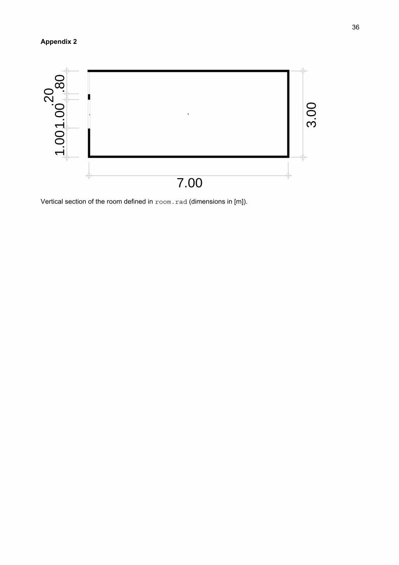
Model of a room daylit by an anidolic light-shelf The basic principles of RADIANCE have been introduced. Now we consider a more detailed example of a rectangular simple room (length=7 [m], width=5 [m], height=3 [m]) daylit from the south facade by two openings (see Appendix 2). The lower window offers a direct view to the outside. The upper opening is equipped with an anidolic internal light-shelf [Com93b] [Com94]. For convenience, these elements and their materials are defined in separate .rad files: cie.rad a CIE overcast sky mat.rad definitions of the materials room.rad the room with empty openings system.rad the daylighting system alone (window glasses and the anidolic light-

shelf) Remarks: The system.rad file calls the genrator program genprism to build the curved anidolic reflector at the line: !genprism reflector ashelf ashelf.dat -c -e -l 0 0 5 | \ xform -rx 90 -rz 90 -t 0 0 3 The reflector profile is given in two dimensions as U,V coordinate pairs in the ashelf.dat file. The output of genprism is then passed through the filter program xform that enables the positioning of a scene using translations (option -t) and/or rotations around the axes of the space (options -rx -ry and -rz). The transformations are applied in the same order as they appear on the command line. Caution! command: xform -t 1 0 0 -rz 90 is NOT equivalent to: xform -rz 90 -t 1 0 0 To get the extreme dimensions of a scene file (i.e. its bounding box in the X,Y,Z space), use the following command: getbbox filename.rad Exercise: Prepare the required transformations in order to position a desk (file desk.rad) and a chair (file chair.rad) somewhere in the room. Write the corresponding calls to xform in a new furnish.rad file. Then put the required scene files together in an octree named model0.oct and make a picture of this model using rview and the following view options: -vp (viewpoint), -vd (view direction), -vh (horizontal view angle) and -vv (vertical view angle). Important: choose a view point and a view direction in order to have the openings in the field of view! To check the relative positions of the desk and the chair, use the objview program that will quickly display the scene: objview furnish.rad

15

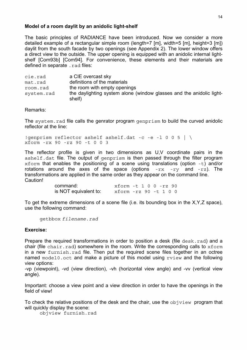
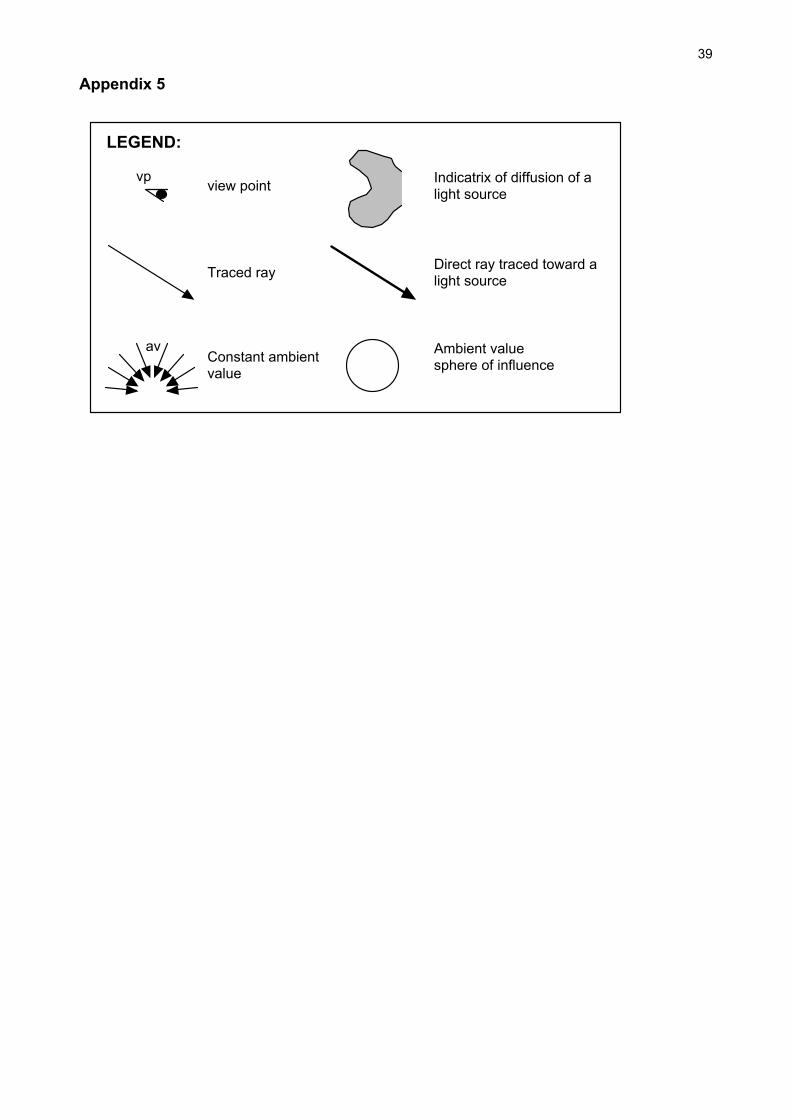
How ray tracing works within RADIANCE The first results are not really convincing. This points out the main difficulty of using RADIANCE: how to control the ray tracing process in order to obtain good results. Many adjustable parameters have to be properly set to achieve this goal and the following section will explain, step by step, how the principal parameters modify the ray tracing process. The symbols used in the graphics are defined in Appendix 5. STEP 1: In the preceding example, rview was started without specifying any ray tracing parameter; this means that neither light coming through interreflections nor a constant ambient illuminance is taken into account (by default rview uses options -ab 0 and -av 0 0 0). In addition the model does not include any light source (the glow material type used to model the sky is usually not considered as a light source!). Finally the sky seen through the openings is the only thing that appears in the picture.

-ab 0 (no interreflections)-av 0 0 0 (no ambient value)

vp

STEP 2: Now in a second attempt an ambient value is set and is supposed constant over the entire scene. This value is specified using option -av that needs three radiances Rr, Rg and Rb as parameters. Usually the ambient value is not coloured so that Rr=Rg=Rb=Ramb. Assuming a constant ambient illuminance Eamb expressed in [lux], Ramb is calculated as:

R Eamb

amb=⋅179 π

Exercise: Calculate an appropriate ambient value for the scene and start rview again adding the corresponding -av option after the same view options as before.

16

-ab 0-av .889 .889 .889 (ambient value set to 500 lux)

vp

av

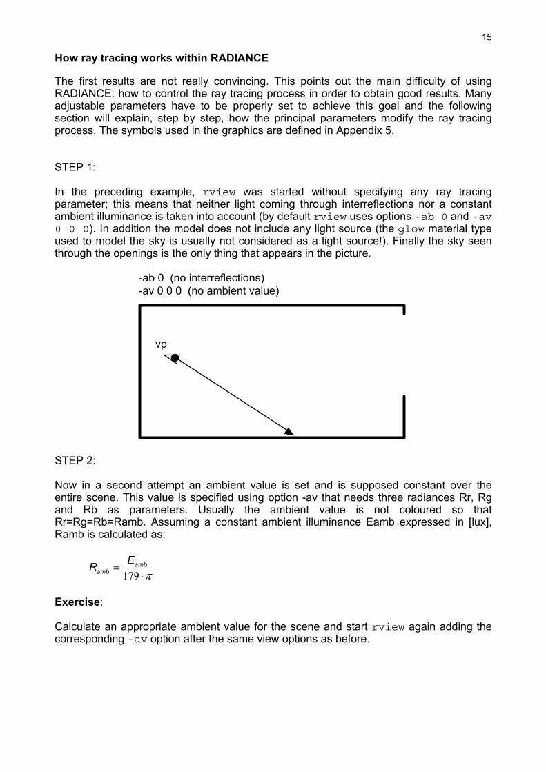
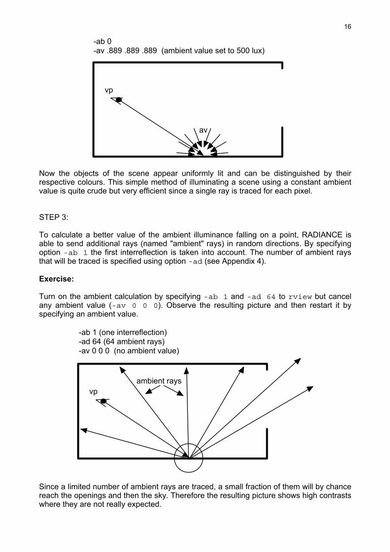
Now the objects of the scene appear uniformly lit and can be distinguished by their respective colours. This simple method of illuminating a scene using a constant ambient value is quite crude but very efficient since a single ray is traced for each pixel. STEP 3: To calculate a better value of the ambient illuminance falling on a point, RADIANCE is able to send additional rays (named "ambient" rays) in random directions. By specifying option -ab 1 the first interreflection is taken into account. The number of ambient rays that will be traced is specified using option -ad (see Appendix 4). Exercise: Turn on the ambient calculation by specifying -ab 1 and -ad 64 to rview but cancel any ambient value (-av 0 0 0). Observe the resulting picture and then restart it by specifying an ambient value.

-ab 1 (one interreflection)-ad 64 (64 ambient rays)-av 0 0 0 (no ambient value)

vpambient rays

Since a limited number of ambient rays are traced, a small fraction of them will by chance reach the openings and then the sky. Therefore the resulting picture shows high contrasts where they are not really expected.

17

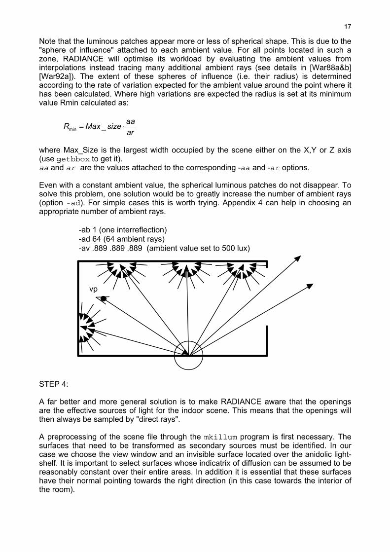
Note that the luminous patches appear more or less of spherical shape. This is due to the "sphere of influence" attached to each ambient value. For all points located in such a zone, RADIANCE will optimise its workload by evaluating the ambient values from interpolations instead tracing many additional ambient rays (see details in [War88a&b] [War92a]). The extent of these spheres of influence (i.e. their radius) is determined according to the rate of variation expected for the ambient value around the point where it has been calculated. Where high variations are expected the radius is set at its minimum value Rmin calculated as:

R Max size aaarmin _= ⋅

where Max_Size is the largest width occupied by the scene either on the X,Y or Z axis (use getbbox to get it). aa and ar are the values attached to the corresponding -aa and -ar options. Even with a constant ambient value, the spherical luminous patches do not disappear. To solve this problem, one solution would be to greatly increase the number of ambient rays (option -ad). For simple cases this is worth trying. Appendix 4 can help in choosing an appropriate number of ambient rays.

-ab 1 (one interreflection)-ad 64 (64 ambient rays)-av .889 .889 .889 (ambient value set to 500 lux)

vp

STEP 4: A far better and more general solution is to make RADIANCE aware that the openings are the effective sources of light for the indoor scene. This means that the openings will then always be sampled by "direct rays". A preprocessing of the scene file through the mkillum program is first necessary. The surfaces that need to be transformed as secondary sources must be identified. In our case we choose the view window and an invisible surface located over the anidolic light-shelf. It is important to select surfaces whose indicatrix of diffusion can be assumed to be reasonably constant over their entire areas. In addition it is essential that these surfaces have their normal pointing towards the right direction (in this case towards the interior of the room).

18

The two surfaces to transform are described in the system.rad file:

#@mkillum i=trans80 d=223 s=115 m=window trans80 polygon view_window 0 0 12 4.8 0 1 0.2 0 1 0.2 0 2 4.8 0 2 #@mkillum i=void d=1100 s=202 m=illum void polygon illuminator 0 0 12 0.2 1.52412861 2.12004394 0.2 0 3 4.8 0 3 4.8 1.52412861 2.12004394 #@mkillum n

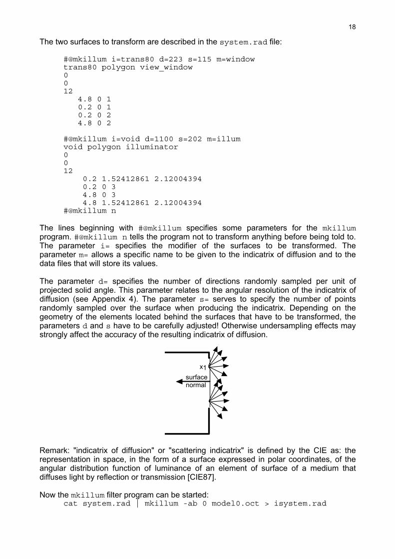
The lines beginning with #@mkillum specifies some parameters for the mkillum program. #@mkillum n tells the program not to transform anything before being told to. The parameter i= specifies the modifier of the surfaces to be transformed. The parameter m= allows a specific name to be given to the indicatrix of diffusion and to the data files that will store its values. The parameter d= specifies the number of directions randomly sampled per unit of projected solid angle. This parameter relates to the angular resolution of the indicatrix of diffusion (see Appendix 4). The parameter s= serves to specify the number of points randomly sampled over the surface when producing the indicatrix. Depending on the geometry of the elements located behind the surfaces that have to be transformed, the parameters d and s have to be carefully adjusted! Otherwise undersampling effects may strongly affect the accuracy of the resulting indicatrix of diffusion.

x1surfacenormal

Remark: "indicatrix of diffusion" or "scattering indicatrix" is defined by the CIE as: the representation in space, in the form of a surface expressed in polar coordinates, of the angular distribution function of luminance of an element of surface of a medium that diffuses light by reflection or transmission [CIE87]. Now the mkillum filter program can be started: cat system.rad | mkillum -ab 0 model0.oct > isystem.rad

19

This process may take a long time. Therefore the resulting file isystem.rad has already been computed. The definition of the window material has for instance been transformed as:

void brightdata window.dist 5 noneg window.dat illum.cal il_alth il_azih 0 9 -1.000000 0.000000 0.000000 0.000000 0.000000 1.000000 0.000000 1.000000 0.000000 window.dist illum window 1 trans80 0 3 5.626943 5.626943 5.626943

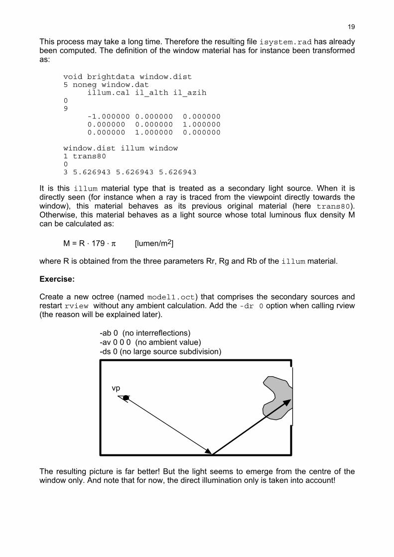
It is this illum material type that is treated as a secondary light source. When it is directly seen (for instance when a ray is traced from the viewpoint directly towards the window), this material behaves as its previous original material (here trans80). Otherwise, this material behaves as a light source whose total luminous flux density M can be calculated as: M = R . 179 . π [lumen/m2] where R is obtained from the three parameters Rr, Rg and Rb of the illum material. Exercise: Create a new octree (named model1.oct) that comprises the secondary sources and restart rview without any ambient calculation. Add the -dr 0 option when calling rview (the reason will be explained later).

-ab 0 (no interreflections)-av 0 0 0 (no ambient value)-ds 0 (no large source subdivision)

vp

The resulting picture is far better! But the light seems to emerge from the centre of the window only. And note that for now, the direct illumination only is taken into account!

20

STEP 5: To correctly treat the window as a large source RADIANCE will automatically split the area of the window into many smaller sources (see detailed explanations in [War94b]). This process is controlled by the option -ds (see Appendix 4 to set an appropriate value). Exercise: Turn on the automatic subdivision of large sources by specifying a value >0 for option -ds and restart the rendering process.

-ab 0 (no interreflections)-av 0 0 0 (no ambient value)-ds 0.3 (large source subdivisions on)

vp

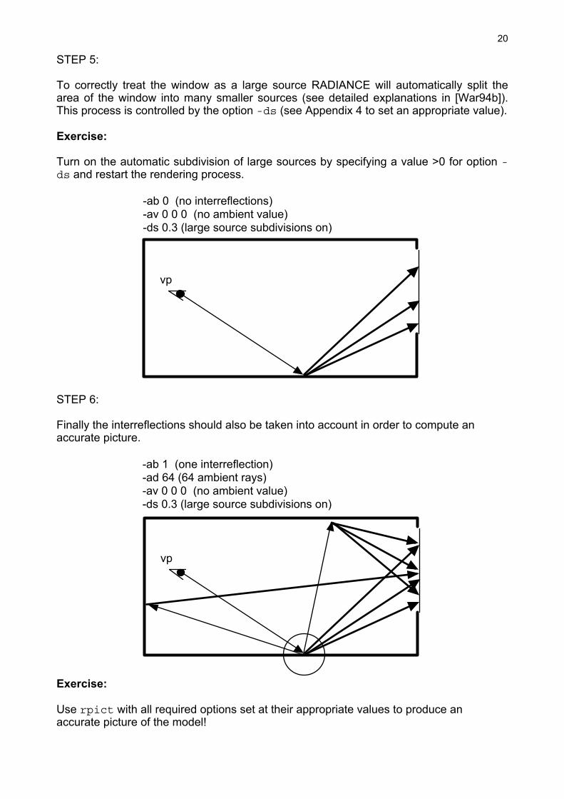
STEP 6: Finally the interreflections should also be taken into account in order to compute an accurate picture.

-ab 1 (one interreflection)-ad 64 (64 ambient rays)-av 0 0 0 (no ambient value)-ds 0.3 (large source subdivisions on)

vp

Exercise: Use rpict with all required options set at their appropriate values to produce an accurate picture of the model!

21

Illuminance calculations RADIANCE is able to compute pictures whose pixels are irradiance values instead of radiance. The option -i of the rendering programs rview and rpict act as switch to this kind of calculation. When looking these pictures using vgaimage or ximage, the values obtained by clicking on specific pixels are either irradiance [W/m2] or illuminance [lux]. Note that this type of picture is totally virtual since it is impossible to produce in the real world. For such pictures, the exposure factor (e) is calculated from a maximum illuminance level Emax in [lux]:

eE

= 179

max

But why spending much time to get a full irradiance picture ? Usually the illuminance falling on a relatively limited number of points is sufficient to know (for instance along an axis in the middle section of the room). The rtrace program called with option -I serves for this purpose. As input it needs a list of the points and orientations where illuminance measurement will be performed. These are provided one per line as two vectors: X Y Z Xdir Ydir Zdir Finally the results of the rtrace program are piped to rcalc in order to compute illuminance values from the three red, green and blue irradiances. This typical series of programs "rtrace -I | rcalc" has been merged into a new single program called rlux. Its parameters are exactly the same as those for the rtrace program but the output results are illuminance levels in [lux]. The call to rillum looks like: cat points.xyz | rlux (rtrace options) model.oct >lux.dat where points.xyz is a file containing the measurement points. The results are written in the output file lux.dat. Exercise Produce an irradiance picture with the same view and ray tracing options as the one just produced before. For the same model use rillum to compute a profile of illuminance levels in the middle section of the room at an height level of 0.8 [m].

22

False colour pictures It is often a good idea to present numerical results using a false colour scale. The falsecolor program is able to perform this task on a RADIANCE picture colouring each pixel according to its radiance value R. The values are mapped to a nice rainbow coloured scale with its lower bound coloured in blue and its upper bound coloured in red. To produce such a picture with a linear scale (always starting from 0), the falsecolor command looks like: falsecolor -i input.pic -s Max_scale -l label -n #divisions >result.pic (This command must be given on a single line) where: input.pic is the picture containing the values that will be mapped to the coloured

scale Max_scale is the luminance or illuminance value of the upper bound of the scale

(every pixel that has higher values will be coloured in red) label is the title that will appear on the top of the coloured scale appended at

the left of the original picture (usually the label refers to the unit of the scale such as [cd/m2] or [lux])

#divisions specifies the number of numerical labels that will be superimposed on the coloured scale

With option -cl the program will instead superimpose #divisions coloured contour lines onto a background picture (specified by option -p): falsecolor -cl -i input.pic -p background.pic -s Max_scale -l label -n #divisions >result.pic This command is very convenient for instance to superimpose isolux curves onto a normal picture of a daylit space. This means that input.pic and background.pic must be of the same size and rendered with the same view parameters but as an illuminance picture for the former (using option -i of either rview or rpict) and as a normal luminance picture for the latter. This kind of resulting picture is of great value because it combines quantitative information (the isolux curves) onto a picture of the space that is less objective (since its exposure can be arbitrarily changed to obtain the desired appearance). Exercise Experience falsecolor using the pictures produced so far.

23

Assessing discomfort glare Discomfort glare is experienced when excessively bright areas are perceived in the field of view. To quantify the sensation of discomfort glare, many "glare indices" have been defined. Nevertheless they are all based on the same kind of parameters. Basically, each excessively bright area is considered as a "source". In fact this reflects the origins of the methods involved which mainly concentrated on artificial lighting installations where each luminaire (= an obvious light source) might create discomfort glare. For daylit scenes, the selection of the parts of the field of view that have to be considered as "sources" is less straightforward. To compute glare indices using RADIANCE, two steps are involved. First the relevant parameters are computed from a calculated picture (or directly from an octree, see [War91b] for details) by the findglare program. The computed parameters are then passed to the glarendx program. First step: findglare -p input.pic -t L_threshold -v >result.gla where: input.pic is a calculated picture taken from the point of view for which discomfort

glare has to be assessed L_threshold is the threshold luminance value in [cd/m2] The threshold value is used by the program to devise which parts must be treated as "sources". Briefly explained, every pixel whose luminance exceed the threshold will first be pinpointed and later merged with neighbouring similar pixels to form individual sources. The resulting parameters describing the positions of the sources found in the picture, the angular extents they subtend (solid angles) and their luminances are finally passed to the output file result.gla. Option -v simply asks the program to print progress reports while running. Second step: glarendx -t index_type input.gla where: index_type is the name of the discomfort glare index to be computed (to get a list of

available indices call glarendx without any argument). The output of glarendx will comprise two numbers: the first column gives the angle between the view direction for which the glare index has been calculated and the original view direction of the input picture (in our case it will always be 0) and the second column is the requested discomfort glare index value. Note that by using option -t vert_ill the glarendx program will return the illuminance measured at the eye level in [lux].

24

Remarks: There is no definitive method to devise appropriate values for the threshold luminance. However, the resulting final discomfort glare indices that strongly depend on the threshold do not have great significance by themselves. They are much more valuable when analysed by comparison with other cases. One possible way of devising a non arbitrary luminance threshold is given by a graph found in reference [Hop70] showing the approximate upper luminance limit under which discomfort glare is not experienced. The corresponding fitted function ulim(La) is the following (contained in the ulim.cal file): fl2cd(v)=3.426*v; cd2fl(v)=.292*v; ulim(La)=fl2cd(10^(5.731+(log10(cd2fl(La))+5)* (0.3376+(log10(cd2fl(La))+5)*0.0189)-6)); The ulim function takes the adaptation luminance La in [cd/m2] as its argument and returns a threshold luminance also in [cd/m2]. The adaptation luminance is not easy to devise for a complex scene since this notion is mainly relevant for experiments on vision where a small target is presented against a background of uniform luminance to which the eyes are adapted. For complex scenes, the adaptation is probably also dependent on the details on which the attention is focused. This is a domain where further reserach is still needed. Anyway, it is common to assume that the illuminance Eeye measured in the scene at eye level is in fact due to a uniform adaptation luminance La over the whole field of view:

LE

aeye=π

[cd/m2]

Then the threshold value can be calculated using the piped commands (given on a single line): findglare -p input.pic -t 100000 | glarendx -h -t vert_ill | rcalc -f ulim.cal -e ‘$1=ulim($2/PI)’ At this stage the very high threshold value used with findglare just ensures that the program does not spend time searching for sources since we just need an illuminance value. Since findglare should normally analyse pictures covering the whole field of view, it is recommended to use hemispherical input pictures (rendered with options -vth -vh 180 -vv 180). Nevertheless, findglare is able to handle pictures covering smaller portions of the field of view. Exercise: Experience discomfort glare calculations using the pictures produced so far.

25

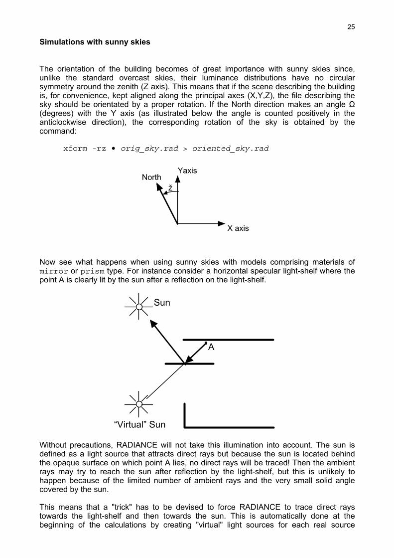
Simulations with sunny skies The orientation of the building becomes of great importance with sunny skies since, unlike the standard overcast skies, their luminance distributions have no circular symmetry around the zenith (Z axis). This means that if the scene describing the building is, for convenience, kept aligned along the principal axes (X,Y,Z), the file describing the sky should be orientated by a proper rotation. If the North direction makes an angle Ω (degrees) with the Y axis (as illustrated below the angle is counted positively in the anticlockwise direction), the corresponding rotation of the sky is obtained by the command: xform -rz • orig_sky.rad > oriented_sky.rad

North

X axis

Yaxis

ž

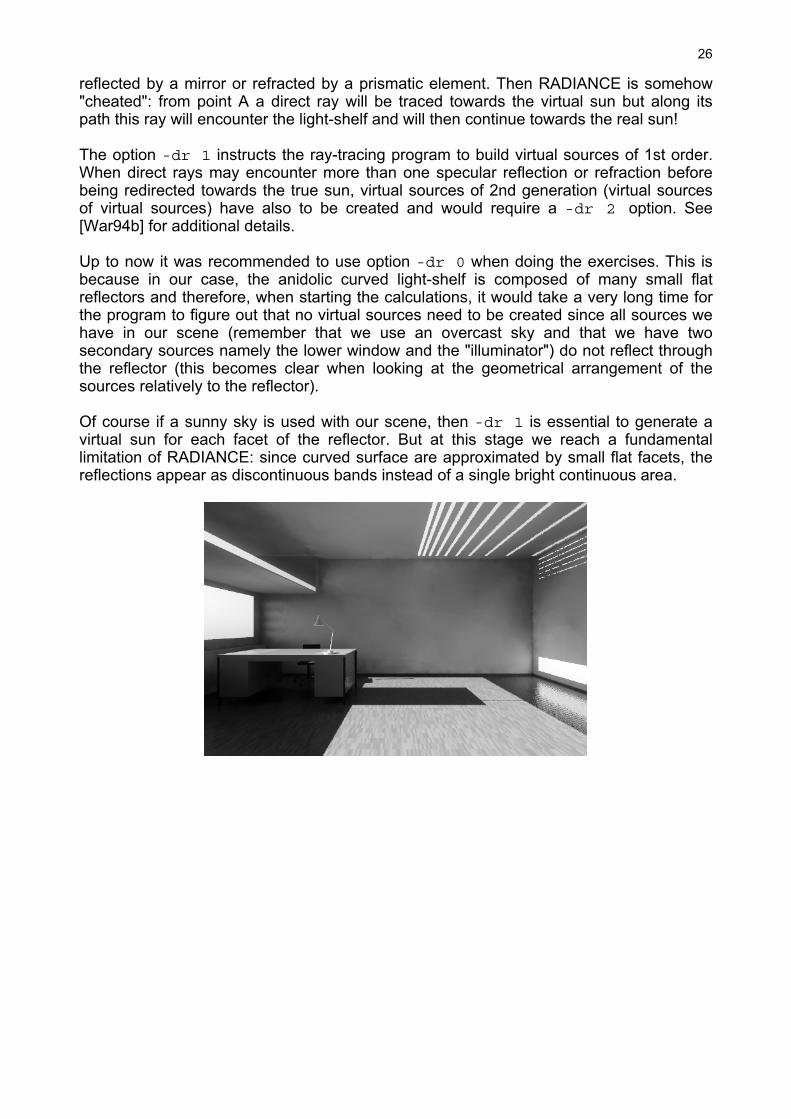
Now see what happens when using sunny skies with models comprising materials of mirror or prism type. For instance consider a horizontal specular light-shelf where the point A is clearly lit by the sun after a reflection on the light-shelf.

A

Sun

“Virtual” Sun

Without precautions, RADIANCE will not take this illumination into account. The sun is defined as a light source that attracts direct rays but because the sun is located behind the opaque surface on which point A lies, no direct rays will be traced! Then the ambient rays may try to reach the sun after reflection by the light-shelf, but this is unlikely to happen because of the limited number of ambient rays and the very small solid angle covered by the sun. This means that a "trick" has to be devised to force RADIANCE to trace direct rays towards the light-shelf and then towards the sun. This is automatically done at the beginning of the calculations by creating "virtual" light sources for each real source

26

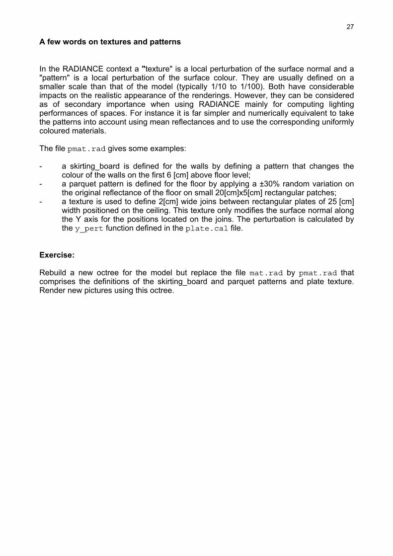
reflected by a mirror or refracted by a prismatic element. Then RADIANCE is somehow "cheated": from point A a direct ray will be traced towards the virtual sun but along its path this ray will encounter the light-shelf and will then continue towards the real sun! The option -dr 1 instructs the ray-tracing program to build virtual sources of 1st order. When direct rays may encounter more than one specular reflection or refraction before being redirected towards the true sun, virtual sources of 2nd generation (virtual sources of virtual sources) have also to be created and would require a -dr 2 option. See [War94b] for additional details. Up to now it was recommended to use option -dr 0 when doing the exercises. This is because in our case, the anidolic curved light-shelf is composed of many small flat reflectors and therefore, when starting the calculations, it would take a very long time for the program to figure out that no virtual sources need to be created since all sources we have in our scene (remember that we use an overcast sky and that we have two secondary sources namely the lower window and the "illuminator") do not reflect through the reflector (this becomes clear when looking at the geometrical arrangement of the sources relatively to the reflector). Of course if a sunny sky is used with our scene, then -dr 1 is essential to generate a virtual sun for each facet of the reflector. But at this stage we reach a fundamental limitation of RADIANCE: since curved surface are approximated by small flat facets, the reflections appear as discontinuous bands instead of a single bright continuous area.

27

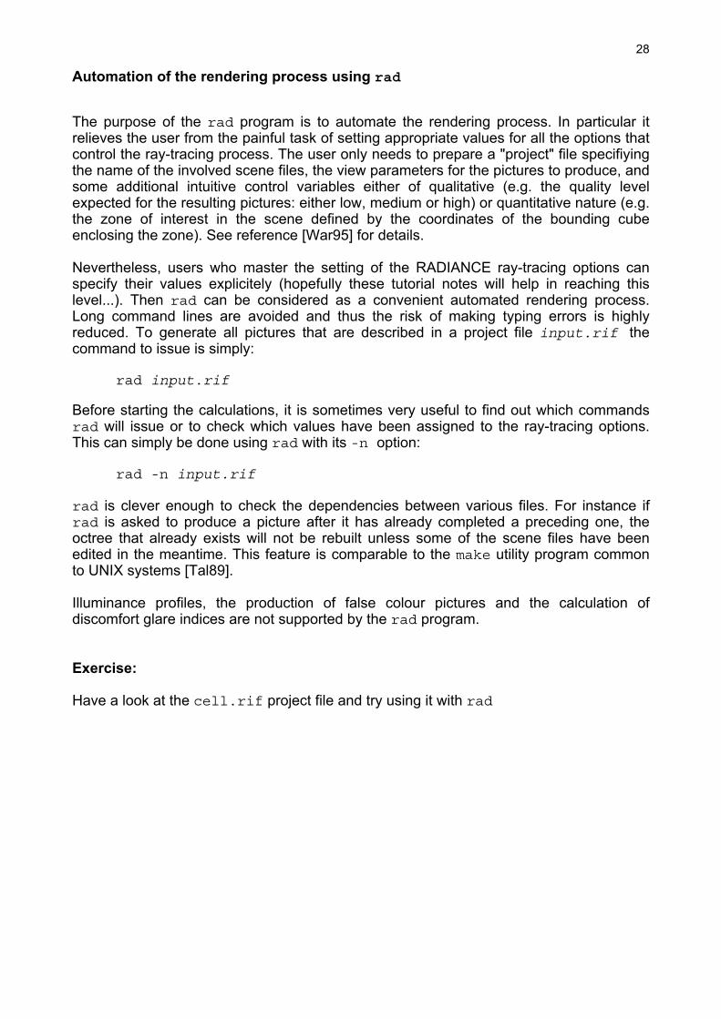
A few words on textures and patterns In the RADIANCE context a "texture" is a local perturbation of the surface normal and a "pattern" is a local perturbation of the surface colour. They are usually defined on a smaller scale than that of the model (typically 1/10 to 1/100). Both have considerable impacts on the realistic appearance of the renderings. However, they can be considered as of secondary importance when using RADIANCE mainly for computing lighting performances of spaces. For instance it is far simpler and numerically equivalent to take the patterns into account using mean reflectances and to use the corresponding uniformly coloured materials. The file pmat.rad gives some examples: - a skirting_board is defined for the walls by defining a pattern that changes the

colour of the walls on the first 6 [cm] above floor level; - a parquet pattern is defined for the floor by applying a ±30% random variation on

the original reflectance of the floor on small 20[cm]x5[cm] rectangular patches; - a texture is used to define 2[cm] wide joins between rectangular plates of 25 [cm]

width positioned on the ceiling. This texture only modifies the surface normal along the Y axis for the positions located on the joins. The perturbation is calculated by the y_pert function defined in the plate.cal file.

Exercise: Rebuild a new octree for the model but replace the file mat.rad by pmat.rad that comprises the definitions of the skirting_board and parquet patterns and plate texture. Render new pictures using this octree.

28

Automation of the rendering process using rad The purpose of the rad program is to automate the rendering process. In particular it relieves the user from the painful task of setting appropriate values for all the options that control the ray-tracing process. The user only needs to prepare a "project" file specifiying the name of the involved scene files, the view parameters for the pictures to produce, and some additional intuitive control variables either of qualitative (e.g. the quality level expected for the resulting pictures: either low, medium or high) or quantitative nature (e.g. the zone of interest in the scene defined by the coordinates of the bounding cube enclosing the zone). See reference [War95] for details. Nevertheless, users who master the setting of the RADIANCE ray-tracing options can specify their values explicitely (hopefully these tutorial notes will help in reaching this level...). Then rad can be considered as a convenient automated rendering process. Long command lines are avoided and thus the risk of making typing errors is highly reduced. To generate all pictures that are described in a project file input.rif the command to issue is simply: rad input.rif Before starting the calculations, it is sometimes very useful to find out which commands rad will issue or to check which values have been assigned to the ray-tracing options. This can simply be done using rad with its -n option: rad -n input.rif rad is clever enough to check the dependencies between various files. For instance if rad is asked to produce a picture after it has already completed a preceding one, the octree that already exists will not be rebuilt unless some of the scene files have been edited in the meantime. This feature is comparable to the make utility program common to UNIX systems [Tal89]. Illuminance profiles, the production of false colour pictures and the calculation of discomfort glare indices are not supported by the rad program. Exercise: Have a look at the cell.rif project file and try using it with rad

29

RADIANCE distribution and user support The RADIANCE UNIX version is freely available on the Internet. The latest version is available by anonymous ftp from: http://radsite.lbl.gov/radiance/ Only the source code is distributed. That means that some computer skills are then necessary to compile and install the software (although an interactive automatic installation procedure is provided). It is worth looking at the RADIANCE-DIGEST (available from the WWW sites) which is a compilation of questions asked by RADIANCE users and the answers given to them. A discussion list is also organised where people using RADIANCE share their problems and (sometimes...) solutions. The currently active list is mainly dedicated to the Desktop RADIANCE version. However general questions regarding RADIANCE are also frequently discussed. To join this list or to browse through its archives connect to:

http://groups.yahoo.com/group/desktopradiance/

The references [War88b] [War91a] [War92a] [War92b] [War94b] [War95] and [War97] are available on the Internet from: http://radsite.lbl.gov/radiance/papers/ The ADELINE package also has dedicated WWW servers but it is not available for free (its price is around 450 US$): http://www.ibp.fhg.de/wt/adeline/ or http://radsite.lbl.gov/adeline/ Each distribution site defines its own policy regarding the user support it offers. The Desktop RADIANCE package is available from: http://radsite.lbl.gov/deskrad/

30

References [CIE87] Commission Internationale de l'Eclairage

Vocabulaire international de l'éclairage Publication CIE n° 17.4, 1987.

[Cla96] J.A. Clarke, J.W. Hand, J. Hensen, K. Johnsen, K. Wittchen, C. Madsen, R. Compagnon

Integrated Performance Appraisal of Daylight-Europe Case Study Buildings Fourth European Conference "Solar Energy in Architecture and Urban Planning", Proceedings, Berlin, Germany, 1996.

[Com92a] R. Compagnon, B. Paule, J.-L. Scartezzini

Etude en éclairage naturel de la nouvelle imprimerie A.B.C. à Schoenbuehl (BE) Publication du CUEPE No 48, Université de Genève, 1992.

[Com92b] R. Compagnon, F. Di Pasquale, B. Paule, J.-L.Scartezzini

Simulation de systèmes d'éclairage naturel complexes 7. Schweizerische Status-Seminar, Energieforschung im Hochbau, ETH-Zürich, 1992.

[Com93a] R. Compagnon, B. Paule, J.-L. Scartezzini

Design of New Daylighting Systems Using Adeline Software Solar Energy in Architecture and Urban Planning, Florence, Italy, 1993.

[Com93b] R. Compagnon, J.-L. Scartezzini, B. Paule

Application of Nonimaging Optics to The Development of New Daylighting systems ISES Solar World Congress, Budapest, Hungary, 1993. (also available on the Internet from the Anidolic Daylighting Systems page: http://lesowww.epfl.ch/daylighting/anidolic-intro.html)

[Com94] R. Compagnon

Simulations numériques de systèmes d’éclairage naturel à pénétration latérale Thèse n° 1193, EPFL, 1994.

[Fro93] K. Frost, M. Donn, R. Amor The Application of RADIANCE to Daylighting Simulation Building Simulation'93, Conference Proceeding, 1993.

[Gry88] A. Grynberg

Comparison and Validation of Radiance and Superlite Internal report, Windows and Daylighting Group, LBL, Berkeley, 1988.

[Gry89] A. Grynberg

Validation d'un programme de simulation d'éclairage: Radiance LBID 1575, LBL, Berkeley, 1989.

[Hop70] R. G. Hopkinson, J. B. Collins

The Ergonomics of Lighting Macdonald & Co. (Publishers) Ltd, London, 1970

[Jem92] F. Jemaa

Dictionnaire bilingue (Anglais/Français) de l’infographie Eyrolles, Paris, 1992.

[Lar98] G. Ward Larson, R. Shakespeare

Rendering with Radiance: the art and science of lighting visualization Morgan Kaufmann Publishers, San Fransisco, 1998.

[Lom93] K. J. Lomas, J. Mardaljevic Advanced daylighting design in atrium buildings Solar Energy in Architecture and Urban Planning, Florence, Italy, 1993.

31

[Mar97] J. Mardaljevic Validation of a Lighting Simulation Program: A Study Using Measured Sky Brightness Distributions Lux Europa 97 Conference Proceedings, 1997.

[Mey86] G. W. Meyer

Tutorial on color science The Visual Computer, 2:278-290, Springer-Verlag,1986.

[Moe96] M. Moeck, E.S. Lee, M.D. Rubin, R. Sullivan, S.E. Selkowitz

Visual Qality Assessment of Electrochromic and Conventional Glazings SPIE Conference "Optical Materials Technology for Energy Efficiency and Solar Energy Conversion XV", Freiburg, Germany, September 1996.

[Nov93] B.J. Novitski

Energy Design Software Architecture, pp. 125-127, June1993.

[Pau92] B.Paule, R. Compagnon, J.-L. Scartezzini

Conception optimale de l'éclairage natuel d'un bâtiment industriel 7. Schweizerische Status-Seminar Energieforschung im Hochbau, ETH-Zürich, 1992.

[Sca94] J.L. Scartezzini, R. Compagnon, G. Ward, B. Paule

Outils informatiques en lumière naturelle Rapport du projet NEFF 435.2, LESO-PB, EPF Lausanne, 1994.

[Tal89] S. Talbott

Managing Projects with Make Nutshell Series, O'Reilly & Associates, 1989.

[War88a] G.J. Ward, F.M. Rubinstein.

A New Technique for Computer Simulation of Illuminated Spaces Journal of the Illuminating Engineering Society, vol. 17, n°1, 1988.

[War88b] G.J. Ward, F.M. Rubinstein, R.D.Clear

A Ray Tracing Solution for Diffuse Interreflection Computer Graphics, vol. 22, n°4, 1988.

[War89] G.J. Ward, F.M. Rubinstein, A. Grynberg

Luminance in Computer - Aided Lighting Design Proceedings of Buildings Simulation '89, Vancouver, 1989.

[War90] G.J. Ward

Visualization Lighting Design + Application (LD+A), vol. 20, n°6, 1990.

[War91a] G.J. Ward

Adaptive Shadow Testing for Ray Tracing Second Eurographics Workshop on Rendering, Barcelona, Spain, 1991.

[War91b] G.J. Ward

RADIANCE Visual Comfort Calculation Rapport interne, LESO, EPFL 1991.

[War91c] G.J. Ward

Real Pixels, Graphics Gems II, Edited by J. Arvo, Academic Press, 1991.

[War92a] G.J. Ward, P.S. Heckbert

Irradiance Gradients Third Eurographics Workshop on Rendering, Bristol, UK, 1992.

[War92b] G.J. Ward

Measuring and Modeling Anisotropic Reflection Computer Graphics, vol. 26, n°2, 1992.

32

[War94a] G.J. Ward

A Contrast-Based Scalefactor for Luminance Display Graphics Gems IV, Edited by P. Eckbert, Academic Press, 1994.

[War94b] G.J. Ward

The Radiance Lighting Simulation and Rendering System Computer Graphics Proceedings, Annual Conference Series, ACM SIGGRAPH, 1994, pp. 459-472

[War94c] G.J. Ward

Applications of RADIANCE to Architecture and Lighting Design IES conference proceedings, 1994.

[War95] G.J. Ward Making Global Illumination User-Friendly Eurographics Workshop on Rendering, 1995.

[War97] G.J. Ward, H. Rushmeier, C. Piatko

A Visibility Matching Tone Reproduction Operator for High Dynamic Range Scenes LBNL report 39882, LBNL Berkeley, 1997.

Acknowledgements This tutorial and its associated example files were originally prepared in January 1996 (in French) for a course requested by the "Architecture et Climat" research group at the University of Louvain-la-Neuve (Belgium). At that time the author was attached to the Laboratoire d'Energie Solaire et de Physique du Bâtiment (LESO-PB) at the Federal Institute of Technology in Lausanne, Switzerland (EPFL). The present English version has been first produced in July 1997 for a course organised by the Low Energy Architecture Research Unit (LEARN) at the University of North London while the author was attached as a visiting associate to the Martin Centre for Architectural and Urban Studies at the University of Cambridge, UK. Many thanks to Jo Dubiel for the assistance provided in the preparation of this document. This slightly revised version has been produced for a course given at EIA-FR. WWW sites of the above mentioned research groups: Martin Centre, Cambridge (UK): http://www.arct.cam.ac.uk/research/index.html LEARN, London (UK): http://www.unl.ac.uk/LEARN/ LESO-PB, Lausanne (Switzerland): http://lesowww.epfl.ch/ Architecture et Climat, Louvain-la Neuve (Belgium): http://www-climat.arch.ucl.ac.be/

33

Appendix 1 Colour "trade"

name Visual appearance Y x y

RAL9010 pure white 0.835 0.328 0.335 2k216 beige 0.71 0.331 0.353 2k218 beige 0.696 0.344 0.369 1k117 off-white 0.688 0.32 0.341 2k217 yellowish 0.683 0.341 0.362 2k205 off-white 0.675 0.33 0.347 6k605 light_gray 0.674 0.317 0.34 4e400 sulfur-yellow 0.673 0.417 0.436 RAL1016 sulfur-yellow 0.673 0.417 0.436 1k105 light_gray 0.667 0.32 0.336 1e101 white-gray 0.666 0.328 0.336 RAL9002 white-gray 0.666 0.328 0.336 1k101 light_gray 0.665 0.323 0.342 2k206 cream 0.665 0.345 0.363 2k201 beige 0.664 0.328 0.349 2k208 beige 0.659 0.352 0.369 7k701 pastel green 0.656 0.316 0.341 1k122 light_gray 0.647 0.322 0.336 2k219 ivory 0.644 0.335 0.359 4k403 beige 0.64 0.362 0.378 7k707 pastel green 0.634 0.327 0.352 1k109 light_gray 0.633 0.314 0.33 4k401 light_yellow 0.629 0.36 0.389 1k113 light_gray 0.628 0.311 0.33 7k709 greenish-white 0.623 0.326 0.349 4k402 yellow 0.621 0.39 0.417 8k801 yellow-green 0.621 0.375 0.431 2k202 beige 0.595 0.336 0.357 6k601 light_blue 0.587 0.307 0.33 2k209 beige 0.584 0.344 0.354 2k220 cream 0.578 0.351 0.375 4k407 yellow 0.572 0.362 0.377 7k710 light_green 0.572 0.322 0.358 1k102 light_gray 0.57 0.322 0.341 4k405 yellow 0.568 0.372 0.39 7k702 green 0.565 0.303 0.343 1k106 light_gray 0.563 0.316 0.332 4k404 yellow 0.56 0.382 0.399 7k704 green 0.55 0.316 0.341 6k608 light_blue 0.548 0.301 0.32 8k804 yellow 0.548 0.449 0.455 1k119 green-gray 0.546 0.318 0.348 6k609 blue-gray 0.541 0.303 0.321 RAL1023 traffic-yellow 0.541 0.449 0.443 1k114 gray 0.533 0.306 0.327 4k408 yellow 0.532 0.375 0.384 1k110 light_gray 0.531 0.312 0.331 2k203 cream 0.527 0.347 0.367 2k222 beige 0.52 0.35 0.373 4k406 ochre-yellow 0.512 0.394 0.399 6k602 light_blue-gray 0.512 0.299 0.32 1k111 light_gray 0.505 0.311 0.329 7k708 green 0.497 0.331 0.373 1k103 light_gray 0.496 0.324 0.343 1k125 beige-gray 0.471 0.339 0.356 3k305 beige-gray 0.464 0.325 0.345 1k120 green-gray 0.462 0.318 0.345

34

8k802 green 0.462 0.385 0.455 4k409 yellow 0.46 0.397 0.425 2k221 greenish-yellow 0.459 0.366 0.392 3k301 light_gray 0.451 0.331 0.345 2k204 beige 0.45 0.351 0.372 2k210 beige 0.443 0.359 0.367 1e123 pebble-gray 0.432 0.337 0.346 RAL7032 pebble-gray 0.432 0.337 0.346 1k107 light_gray 0.432 0.317 0.336 1k104 light_gray 0.43 0.327 0.345 2k213 beige 0.428 0.363 0.376 3k308 beige 0.427 0.344 0.36 7k705 green-blue 0.422 0.31 0.342 1k115 blue-gray 0.418 0.299 0.319 2k223 yellow 0.413 0.358 0.384 7k711 green 0.412 0.315 0.367 6k603 light_blue 0.407 0.286 0.314 2k214 yellow 0.406 0.379 0.395 2k212 brownish-beige 0.398 0.379 0.378 1k124 gray 0.395 0.324 0.337 1k112 gray 0.393 0.306 0.323 1k108 light_gray 0.388 0.317 0.335 2k215 yellow 0.379 0.377 0.397 1k116 blue-gray 0.378 0.298 0.318 4e404 chrome-yellow 0.377 0.464 0.433 RAL1007 chrome-yellow 0.377 0.464 0.433 2k225 brown 0.375 0.377 0.391 4k410 yellow 0.374 0.432 0.413 1k126 gray 0.368 0.335 0.354 1k127 beige 0.367 0.345 0.364 4k411 ochre 0.351 0.426 0.391 2k211 brownish-yellow 0.337 0.37 0.379 7k713 light_green 0.334 0.362 0.4 6k604 blue 0.326 0.281 0.309 RAL2008 light_red-orange 0.323 0.469 0.408 7k712 green 0.315 0.337 0.381 3k306 gray 0.312 0.324 0.346 4k412 orange-beige 0.307 0.427 0.396 7k706 green-blue 0.305 0.309 0.35 3k309 gray 0.3 0.329 0.344 1e121 silver-gray 0.298 0.311 0.321 RAL7001 silver-gray 0.298 0.311 0.321 2k224 olive 0.292 0.368 0.399 7e712 pale green 0.287 0.341 0.364 RAL6021 pale green 0.287 0.341 0.364 2k229 green 0.282 0.352 0.378 2k228 brown 0.28 0.382 0.384 1k128 beige 0.278 0.344 0.363 2k227 brown 0.278 0.385 0.387 2k226 brown 0.264 0.386 0.384 1e122 stone-gray 0.259 0.332 0.34 RAL7030 stone-gray 0.259 0.332 0.34 4k413 orange-brown 0.253 0.441 0.391 8k803 olive 0.251 0.403 0.468 1k129 gray 0.249 0.338 0.362 3k302 light_gray 0.246 0.32 0.341 3k311 gray 0.245 0.326 0.343 4k414 light_brown 0.231 0.423 0.383 5k505 red-brown 0.23 0.391 0.353 7k714 green 0.22 0.354 0.409 RAL6018 yellow-green 0.218 0.376 0.45

35

3k303 gray 0.217 0.321 0.343 8k806 blue 0.209 0.242 0.263 1e105 concrete-gray 0.201 0.332 0.341 RAL7023 concrete-gray 0.201 0.332 0.341 8k805 orange-red 0.197 0.467 0.361 3k310 gray 0.184 0.331 0.346 3k312 brown-gray 0.179 0.347 0.356 3k313 beige-brown 0.179 0.349 0.359 7e704 reseda-green 0.169 0.349 0.379 RAL6011 reseda-green 0.169 0.349 0.379 5e520 lilac-blue 0.169 0.277 0.264 RAL4005 lilac-blue 0.169 0.277 0.264 3k307 gray 0.169 0.328 0.35 RAL2002 blood-orange 0.162 0.485 0.392 3k304 dark_gray 0.149 0.329 0.346 1k130 gray 0.147 0.308 0.337 1k134 dark_gray 0.138 0.302 0.315 RAL6024 traffic-green 0.133 0.318 0.398 1e119 blue-gray 0.121 0.304 0.317 RAL7031 blue-gray 0.121 0.304 0.317 5e509 fire-red 0.119 0.473 0.381 RAL3000 fire-red 0.119 0.473 0.381 7e706 emerald-green 0.086 0.351 0.427 RAL6001 emerald-green 0.086 0.351 0.427 RAL6016 turquoise-green 0.079 0.285 0.364 7e711 olive-green 0.071 0.36 0.381 RAL6003 olive-green 0.071 0.36 0.381 RAL5017 traffic-blue 0.069 0.177 0.199 5e504 ruby-red 0.065 0.488 0.376 RAL3003 ruby-red 0.065 0.488 0.376 6e610 gentian-blue 0.052 0.183 0.196 RAL5010 gentian-blue 0.052 0.183 0.196 RAL4004 bordeaux-violet 0.042 0.408 0.32 5e505 red-brown 0.042 0.467 0.368 RAL3004 red-brown 0.042 0.467 0.368 RAL5002 ultramarine 0.039 0.171 0.162 3e311 mahogany-brown 0.032 0.415 0.381 RAL8016 mahogany-brown 0.032 0.415 0.381 5e506 wine-red 0.029 0.45 0.359 RAL3005 wine-red 0.029 0.45 0.359 RAL4007 purple-violet 0.027 0.342 0.291 6e605 sapphire-blue 0.026 0.202 0.207 RAL5003 sapphire-blue 0.026 0.202 0.207 RAL5022 midnight-blue 0.023 0.197 0.184

36

Appendix 2

1.00

1.00

.80

.20

3.00

7.00 Vertical section of the room defined in room.rad (dimensions in [m]).

37

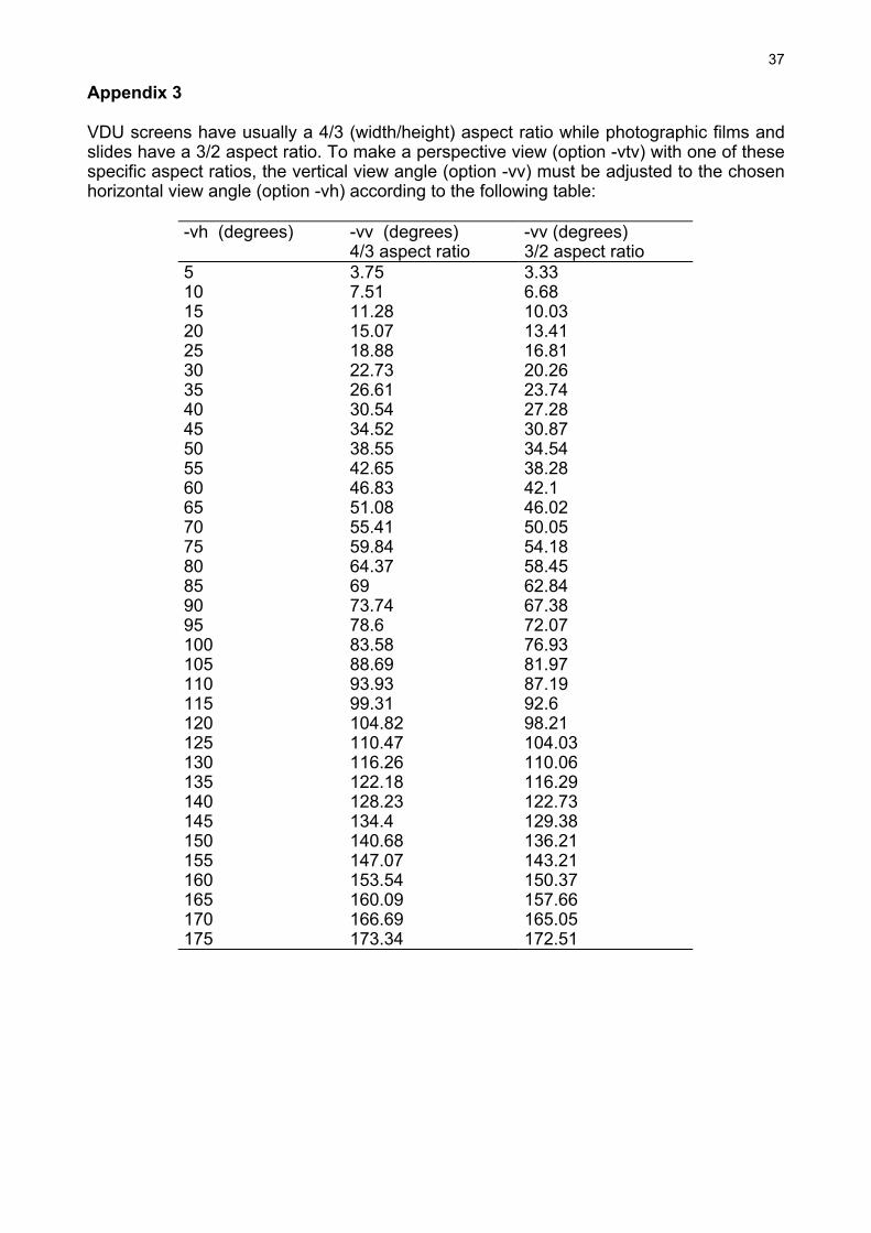
Appendix 3 VDU screens have usually a 4/3 (width/height) aspect ratio while photographic films and slides have a 3/2 aspect ratio. To make a perspective view (option -vtv) with one of these specific aspect ratios, the vertical view angle (option -vv) must be adjusted to the chosen horizontal view angle (option -vh) according to the following table:

-vh (degrees) -vv (degrees) 4/3 aspect ratio

-vv (degrees) 3/2 aspect ratio

5 3.75 3.33 10 7.51 6.68 15 11.28 10.03 20 15.07 13.41 25 18.88 16.81 30 22.73 20.26 35 26.61 23.74 40 30.54 27.28 45 34.52 30.87 50 38.55 34.54 55 42.65 38.28 60 46.83 42.1 65 51.08 46.02 70 55.41 50.05 75 59.84 54.18 80 64.37 58.45 85 69 62.84 90 73.74 67.38 95 78.6 72.07 100 83.58 76.93 105 88.69 81.97 110 93.93 87.19 115 99.31 92.6 120 104.82 98.21 125 110.47 104.03 130 116.26 110.06 135 122.18 116.29 140 128.23 122.73 145 134.4 129.38 150 140.68 136.21 155 147.07 143.21 160 153.54 150.37 165 160.09 157.66 170 166.69 165.05 175 173.34 172.51

38

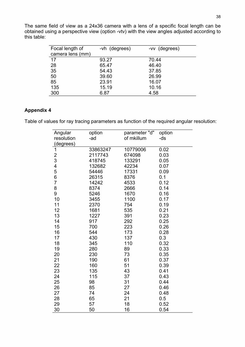
The same field of view as a 24x36 camera with a lens of a specific focal length can be obtained using a perspective view (option -vtv) with the view angles adjusted according to this table:

Focal length of camera lens (mm)

-vh (degrees) -vv (degrees)

17 93.27 70.44 28 65.47 46.40 35 54.43 37.85 50 39.60 26.99 85 23.91 16.07 135 15.19 10.16 300 6.87 4.58

Appendix 4 Table of values for ray tracing parameters as function of the required angular resolution:

Angular resolution (degrees)

option -ad

parameter "d" of mkillum

option -ds

1 33863247 10779006 0.02 2 2117743 674098 0.03 3 418745 133291 0.05 4 132682 42234 0.07 5 54446 17331 0.09 6 26315 8376 0.1 7 14242 4533 0.12 8 8374 2666 0.14 9 5246 1670 0.16 10 3455 1100 0.17 11 2370 754 0.19 12 1681 535 0.21 13 1227 391 0.23 14 917 292 0.25 15 700 223 0.26 16 544 173 0.28 17 430 137 0.3 18 345 110 0.32 19 280 89 0.33 20 230 73 0.35 21 190 61 0.37 22 160 51 0.39 23 135 43 0.41 24 115 37 0.43 25 98 31 0.44 26 85 27 0.46 27 74 24 0.48 28 65 21 0.5 29 57 18 0.52 30 50 16 0.54

39

Appendix 5

av

vp

LEGEND:

view point

Traced ray

Constant ambient value

Ambient value sphere of influence

Direct ray traced toward a light source

Indicatrix of diffusion of a light source