r a d i o n a v i g a t i o n ( a n o v e r v i e w )

Low frequencies were very important to air navigation years ago, but became increasingly less important as more reliable systems operating at higher frequencies were developed and became widely available. Many Low Frequency navigation beacons were decommissioned long ago because of that. The few that remain primarily provide backup navigation in the event of primary navigation system failures, although some are used routinely even today in the execution of instrument landings.

Long ago, before VHF Omnirange (VOR) and other superior navigation systems were developed, that band contained AN Radio Ranges and Non-Directional Beacons (NDB's). 344 AN Radio Ranges still existed in the United States in 1959, but none exist today. Some NDB's are all that remain.

The Low Frequency (LF) aviation band extends from 200 kHz to 415 kHz with some internal gaps assigned to other services. The entire Low Frequency (LF) aviation band can be received by the receiver at this website.

Medium Frequency Aviation Band Usage

The only portion of the Medium Frequency spectrum allocated for aviation use is the 2850 to 3000 kHz portion of the 2850 to 3155 kHz Aviation Band. However, most aircraft are equipped with radio direction finders than can receive Medium Frequency AM Broadcast Band.

High Frequency (HF) Aviation Bands

High Frequencies were widely used for domestic aircraft voice communications years ago. Nearly all that traffic moved to Very High Frequencies long ago and domestic aircraft use of Medium Frequencies is now very rare. However, international flights still use the High Frequencies bands routinely for voice communications, because of the much longer distances over which they can be used.

Radio navigation provides the pilot with position information from ground stations located worldwide. There are several systems offering various levels of capability with features such as course correction information, automatic direction finder and distance measuring.

Most aircraft now are equipped with some type of radio navigation equipment. Almost all flights whether cross-country or "around the patch" use radio navigation equipment in some way as a primary or secondary navigation aid.

Table of Radio Frequencies

Description Abbreviation Frequency Wavelength

Very Low Frequency VLF 3 KHz - 30 KHz 100,000m -

10,000m

Low Frequency LF 30 KHz - 300 KHz 10,000m - 1,000

Medium Frequency MF 300 KHz - 3 MHz 1,000m - 100m

High Frequency HF 3 MHz - 30 MHz 100m - 10m

Very High Frequency VHF 30 MHz - 300

MHz 10m - 1m

Ultra High Frequency UHF 300 MHz - 3 GHz 1m - 0.10m

Super High Frequency SHF 3 GHz - 30 GHz 0.10m - 0.01m

Extremely High Frequency EHF 30 GHz - 300

GHz 0.01m - 0.001m

The fact that radio signals can travel all over the globe on the HF bands is widely used from radio hams to broadcasters and maritime applications to diplomatic services. Radio transmitters using relatively low powers can be used to communicate to the other side of the globe. Although this form of communication is not as reliable as satellites, radio hams enjoy the possibility of making these contacts when they occur. Other users need to be able to establish more reliable communications. In doing this they make extensive use of propagation programmes to predict the regions to which signals will travel, or the probability of them reaching a given area.

These propagation prediction programmes utilise a large amount of data, and many have been developed over many years. However it is still useful to gain a view of how signals travel on these frequencies, to understand why signal conditions change and how the signals propagate at these frequencies.

Radio signals in the medium and short wave bands travel by two basic means. The first is known as a ground wave, and the second a sky wave.

Ground Wave

Ground wave radio propagation is used mainly on the medium wave band. It might be expected that the signal would travel out in a straight line. However it is affected by the proximity of the earth it is found that the signal tends to follow the earth's curvature. This occurs because currents are induced in the surface of the earth and this slows down the wave front close to the ground. This results in the wave front tilting downward, enabling it to follow the curvature of the earth and travel beyond the horizon.

 Ground wave propagation

Ground wave propagation becomes less effective as the frequency rises. The distances over which signals can be heard steadily reduce as the frequency rises, to the extent that even high power short wave stations may only be heard over a few kilometres via this mode of propagation. Accordingly it is only used for signals below about 2 or 3 MHz. In comparison medium wave stations are audible over much greater distances - typically the coverage area for a high power broadcast station may extend out a hundred kilometres or more. The actual coverage is affected by a variety of factors including the transmitter power, the type of antenna, and the terrain over which the signal is travelling.

Signals also leave the earth's surface and travel towards the ionosphere, some of these are returned to earth. These signals are termed sky waves for obvious reason.D layer

When a sky wave leaves the earth's surface and travels upwards, the first layer of interest that it reaches in the ionosphere is called the D layer. This layer attenuates the signals as they pass through. The level of attenuation depends on the frequency. Low frequencies are attenuated more than higher ones. In fact it is found that the attenuation varies as the inverse square of the frequency, i.e. doubling the frequency reduces the level of attenuation by a factor of four. This means that low frequency signals are often prevented from reaching the higher layers, except at night when the layer disappears.

The D layer attenuates signals because the radio signals cause the free electrons in the layer to vibrate. As they vibrate the electrons collide with molecules, and at each collision there is a small loss of energy. With countless millions of electrons vibrating, the amount of energy loss becomes noticeable and manifests itself as a reduction in the overall signal level. The amount of signal loss is dependent upon a number of factors: One is the number of gas molecules that are present. The greater the number of gas molecules, the higher the number of collisions and hence the higher the attenuation. The level of ionisation is also very important. The higher the level of ionisation, the greater the number of electrons that vibrate and collide with molecules. The third main factor is the frequency of the signal. As the frequency increases, the wavelength of the vibration shortens, and the number of collisions between the free electrons and gas molecules decreases. As a result signals lower in the frequency spectrum are attenuated far more than those which are higher in frequency. Even so high frequency signals still suffer some reduction in signal strength.E and F Layers

Once a signal passes through the D layer, it travels on and reaches first the E, and next the F layers. At the altitude where these layers are found the air density is very much less, and this means that when the free electrons are excited by radio signals and vibrate, far fewer collisions occur. As a result the way in which these layers act is somewhat different. The electrons are again set in motion by the radio signal, but they tend to re-radiate it. As the signal is travelling in an area where the density of electrons is increasing, the further it

progresses into the layer, the signal is refracted away from the area of higher electron density. In the case of HF signals, this refraction is often sufficient to bend them back to earth. In effect it appears that the layer has "reflected" the signal.

The tendency for this reflection is dependent upon the frequency and the angle of incidence. As the frequency increases, it is found that the amount of refraction decreases until a frequency is reached where the signals pass through the layer and on to the next. Eventually a point is reached where the signal passes through all the layers and on into outer space. 

Refraction of a signal as it enters an ionised layer

Different frequencies

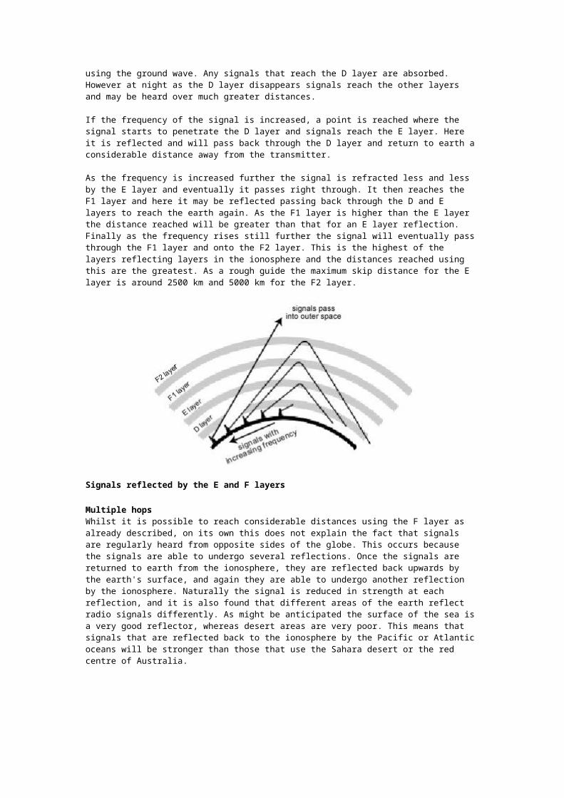
To gain a better idea of how the ionosphere acts on radio signals it is worth viewing what happens to a signal if the frequency is increased across the frequency spectrum. First it starts with a signal in the medium wave broadcast band. During the day signals on these frequencies only propagate using the ground wave. Any signals that reach the D layer are absorbed. However at night as the D layer disappears signals reach the other layers and may be heard over much greater distances.

If the frequency of the signal is increased, a point is reached where the signal starts to penetrate the D layer and signals reach the E layer. Here it is reflected and will pass back through the D layer and return to earth a considerable distance away from the transmitter.

As the frequency is increased further the signal is refracted less and less by the E layer and eventually it passes right through. It then reaches the F1 layer and here it may be reflected passing back through the D and E layers to reach the earth again. As the F1 layer is higher than the E layer the distance reached will be greater than that for an E layer reflection.Finally as the frequency rises still further the signal will eventually pass through the F1 layer and onto the F2 layer. This is the highest of the layers reflecting layers in the ionosphere and the distances reached using this are the greatest. As a rough guide the maximum skip distance for the E layer is around 2500 km and 5000 km for the F2 layer.

Signals reflected by the E and F layers

Multiple hopsWhilst it is possible to reach considerable distances using the F layer as already described, on its own this does not explain the fact that signals are regularly heard from opposite sides of the globe. This occurs because the signals are able to undergo several reflections. Once the signals are returned to earth from the ionosphere, they are reflected back upwards by the earth's surface, and again they are able to undergo another reflection by the ionosphere. Naturally the signal is reduced in strength at each reflection, and it is also found that different areas of the earth reflect radio signals differently. As might be anticipated the surface of the sea is a very good reflector, whereas desert areas are very poor. This means that signals that are reflected back to the ionosphere by the Pacific or Atlantic oceans will be stronger than those that use the Sahara desert or the red centre of Australia.

Multiple reflections

It is not just the earth's surface that introduces losses into the signal path. In fact the major cause of loss is the D layer, even for frequencies high up into the HF portion of the spectrum. One of the reasons for this is that the signal has to pass through the D layer twice for every reflection by the ionosphere. This means that to get the best signal strengths it is necessary signal paths enable the minimum number of hops to be used. This is generally achieved using frequencies close to the maximum frequencies that can support ionospheric communications, and thereby using the highest layers in the ionosphere. In addition to this the level of attenuation introduced by the D layer is also reduced. This means that a signal on 20 MHz for example will be stronger than one on 10 MHz if propagation can be supported at both frequencies.

A VOR is a Very-high-frequency OmniRange radio transmitter. VORs constitute the backbone of current land-based aerial navigation in the U.S. and Western Europe. But first, let's start with the NDB because it's a simpler device.

NDB

An NDB (Non-Directional Beacon) is a radio beacon that broadcasts continuously on a specific frequency. Aircraft on-board radio equipment can determine in which direction from the aircraft an NDB signal is coming. The on-board aerial consists of a simple metal loop which is rotatable. The radio signal induces a current in the loop, as in a normal aerial, but this current is weaker or stronger depending on the orientation of the loop. When the loop is flat-on to the origin of the signal, the signal is strongest. (Think of the loop as the frame of a round mirror. The signal is detected to be strongest when the mirror is reflecting it back at itself.) The official definition is

A L/MF [low- or medium-frequency] or UHF [ultra-high-frequency] radio beacon transmitting non-directional signals whereby the pilot of an aircraft equipped with direction finding equipment can determine his bearing to or from the radio beacon and "home" on or track from the station. When the radio beacon is installed in conjunction with the Instrument Landing System marker, it is normally called a Compass Locator.,

in which bearing means:

The horizontal direction to or from any point, usually measured clockwise from true north, magnetic north, or some other reference point through 360 degrees.

Because aircraft can determine from which direction the signal is coming, they can `home in on', fly in the direction of, the signal to arrive at the beacon.

NDBs broadcast in the frequency band of 190 to 535kHz (a `Hertz', Hz, is one cycle per second) and transmit a continuous carrier signal with either 400 or 1020 Hz modulation. An identification signal consisting of three letters in Morse code is also transmitted. The receiver equipment in the airplane is called an ADF (`Automatic Direction Finder'). The indicator consists of a round calibrated dial and a `needle' pointer which points in the direction that the signal is determined to be coming from.

There are two problems with NDBs. First, erroneous signals.

Radio beacons are subject to disturbances that may result in erroneous bearing information. Such disturbances result from such factors as lightning, precipitation static, etc. At night radio beacons are vulnerable to interference from distant stations. Noisy identification usually occurs when the ADF needle is erratic. Voice, music or erroneous identification may be heard when a steady false bearing is being displayed. Since ADF receivers do not have a "flag" to warn the pilot when erroneous bearing information is being displayed, the pilot should continuously monitor the NDB's identification. 

Second, you can only tell the relative bearing of your aircraft to the NDB - that is, the direction in which the NDB lies. Only by comparing this against the aircraft compass heading (as stably indicated by the directional gyroscope) and doing some trivial trigonometry in his/her head can a pilot determine at which (magnetic or true) bearing the NDB lies from the aircraft. This can be illustrated thus:

The circular black dial with indicator in the middle of the aircraft is what the pilot sees inside the aircraft.

Some aircraft have an instrument called an RMI (Radio Magnetic Indicator) which incorporates both a directional gyro and the ADF needle so that one can read the magnetic bearing to the beacon directly off the instrument without having to do mental trigonometry.

The service range of an NDB is the distance from the NDB within which a reliable signal is guaranteed. Service ranges are classified as 15, 25, 50 and 75 nautical miles.

NDB Navigation

NDB navigation is not necessarily easy. First, there is a course to be flown. Second, the aircraft may be on-course or slightly (or hugely) off-course. Thirdly, the heading of the aircraft may be different from track, to accommodate a crosswind. During an instrument approach, a pilot has to continuously determine all this information, and also calculate and fly corrections. Determining which heading to hold to accommodate a crosswind is an empirical matter. One guesses a heading and determines drift (range of divergence of track from course) and then corrects - first twice as much, to get back onto course, and then when back on course, enough to follow course. All this is quite tricky and one needs to be in practice. This is crucial when flying an instrument approach, since strict adherence to course and altitude restrictions are the only things that guarantee that the aircraft flies clear of obstacles. Anybody who has flown an NDB instrument approach to an airport runway knows how labour-intensive it is. One has to achieve course-following using the above procedure, correcting for probably-changing crosswinds as one descends in altitude, especially in non-level terrain, very accurately and all inside of 2 or 3 minutes.

Use of an ADF in NDB navigation can be illustrated thus:

The aircraft is flying on a course directly from the beacon. We don't know what azimuth this course has, but the dial on the ADF is set to straight-ahead=0° (on an RMI, there would be a directional gyro indicator here, not a settable dial). There is a crosswind coming from the left, so a heading correction to the left of 030° must be taken to maintain course in the

crosswind. This heading correction shows up on the ADF, indicating that the beacon is relatively at a bearing of 210° behind the aircraft, which means with the heading correction for crosswind, that we are flying on a course with the beacon at a bearing of 180° to our course behind us.

The solution to NDB navigation problems is the VOR.

VORs

VHF Omni-directional Radio (VORs) are radio beacons that transmit an signal which contains precise azimuth information, so that upon reception of the signal, an aircraft can tell precisely what bearing with respect to magnetic north the station is from the aircraft (respectively, on what radial the aircraft lies from the station - this is just the reciprocal of the bearing to the station from the aircraft). Such a signal has the advantage that the bearing to the station is read directly off the indicator equipment. `The accuracy of course alignment of the VOR is excellent, being generally plus or minus 1 degree'

Navigating on VOR information is akin to flying on a grid such as the following:

Here, the aircraft is positioned directly on the 315° radial from the VOR. (We do not know on what course the aircraft is flying, although its heading appears to be about 350°.)

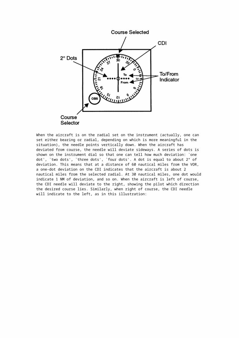
Besides being very accurate, the VOR is much easier to use than an NDB. The indicator in the cockpit is a round dial with settable azimuth information, called the Omni Bearing Selector (OBS) and a vertical pendulum-like needle, called the Course Deviation Indicator (CDI) thus:

When the aircraft is on the radial set on the instrument (actually, one can set either bearing or radial, depending on which is more meaningful in the situation), the needle points vertically down. When the aircraft has deviated from course, the needle will deviate

sideways. A series of dots is shown on the instrument dial so that one can tell how much deviation: `one dot', `two dots', `three dots', `four dots'. A dot is equal to about 2° of deviation. This means that at a distance of 60 nautical miles from the VOR, a one-dot deviation on the CDI indicates that the aircraft is about 2 nautical miles from the selected radial. At 30 nautical miles, one dot would indicate 1 NM of deviation, and so on. When the aircraft is left of course, the CDI needle will deviate to the right, showing the pilot which direction the desired course lies. Similarly, when right of course, the CDI needle will indicate to the left, as in this illustration:

In this diagram, the OBS is set to 0°=360°. An aircraft in position A, B, or C will show a deviation on the CDI as shown to the right (but somewhat exaggerated - the precise number of dots shows a 4° deviation, and the positions A, B, C are indicated much more than 4° to the right of course). Aircraft with 0° set in the OBS, to the south of the VOR in positions D and E, will show a similar deviation. It is important to realise that, unlike with an ADF display, the VOR indicator (OBS and CDI) shows position over the ground with respect to the VOR, and independent of heading or course.

Thus position information along a radial from a VOR is shown directly and accurately on the VOR indicator and there is no need to follow the complicated procedures involved in NDB navigation. One can determine absolute position by tuning two VOR receivers to two different VORs, determining (by centring both DCIs) on what radial from each VOR the aircraft currently lies, and then drawing these two extended radials on the chart on one's knee (the radials are shown on the chart for each VOR, but they don't extend very far from the VOR) to see where they intersect, and that's where the aircraft is!

There are some devices called RNAV which integrate such information from two or more VORs to construct a `virtual VOR' on any chosen course, so that to fly this course, one just centres the CDI needle on the indicator, as though there were actually a VOR one is flying towards. RNAVs are nice.

VOR navigation is the major navigation technique throughout much of the world, and certainly in developed countries such as the U.S. and Western Europe. It was developed a half-century ago, after the Second World War.

Technically, VOR operation is achieved by transmitting two signals (actually, there is a continuous carrier with modulation, but let us for the moment consider it as a discrete signal). The base signal is transmitted at regular intervals, let us say time interval T, and in between base signals occurs an azimuth signal. The difference in time between base signal

and azimuth signal determines the radial azimuth (from magnetic north) from the VOR that the aircraft is on. When the aircraft is due (magnetic) north of the VOR, the two signals coincide. As the radial angle increases clockwise, the signals become further and further apart. For example, at 90°, the azimuth signal will be at 0.25T; at 180°, at 0.5T; at 270°, 0.75T, until when at magnetic north again, the two signals again coincide.

VOR reception is line-of-sight. `VORs operate within the 108.0 to 117.95 MHz frequency band, and have a power output necessary to provide coverage within their assigned operational service volume'. The service volumes are given by the class of VOR:

T (Terminal): From 1000 feet above ground level (AGL) up to and including 12,000 feet AGL at radial distances out to 25 NM;

L (Low Altitude): From 1000 ft AGl up to and including 18,000 feet AGL at radial distances out to 40 NM;

H (High Altitude): From 1000 feet AGL up to and including 14,500 feet AGL at radial distances out to 40 NM. From 14,500 AGL up to and including 60,000 feet at radial distances out to 100 NM. From 18,000 feet AGL up to and including 45,000 feet AGL at radial distances out to 130 NM.

Finally, many aircraft (and most commercial transports) have an instrument that combines a directional gyroscope with a VOR receiver, called a Horizontal Situation Indicator (HSI) and which looks like this:

Instrument Landing System (ILS)

An aircraft on an instrument landing approach has a cockpit with computerized instrument landing equipment that receives and interprets signals being from strategically placed stations on the ground near the runway. This system includes a "Localizer" beam that uses the VOR indicator with only one radial aligned with the runway. The Localizer beam's width is from 3° to 6°. It also uses a second beam called a "glide slope" beam that gives vertical information to the pilot. The glide slope is usually 3° wide with a height of 1.4°. A horizontal needle on the VOR/ILS head indicates the aircraft's vertical position. Three marker beacons (outer, middle and inner) are located in front of the landing runway and indicate their distances from the runway threshold. The Outer Marker (OM) is 4 to 7 miles from the runway. The Middle Marker (MM) is located about 3,000 feet from the landing threshold, and the Inner Marker (IM) is located between the middle marker and the runway threshold

where the landing aircraft would be 100 feet above the runway.

The VOR indicator for an ILS system uses a horizontal needle in addition to the vertical needle. When the appropriate ILS frequency is entered into the navigation radio, the horizontal needle indicates where the aircraft is in relation to the glide slope. If the needle is above the centre mark on the dial, the aircraft is below the glide slope. If the needle is below the centre mark on the dial, the aircraft is above the glide slope.

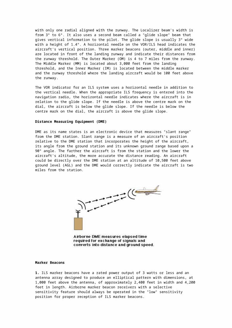
Distance Measuring Equipment (DME)

DME as its name states is an electronic device that measures "slant range" from the DME station. Slant range is a measure of an aircraft's position relative to the DME station that incorporates the height of the aircraft, its angle from the ground station and its unknown ground range based upon a 90° angle. The farther the aircraft is from the station and the lower the aircraft's altitude, the more accurate the distance reading. An aircraft could be directly over the DME station at an altitude of 10,500 feet above ground level (AGL) and the DME would correctly indicate the aircraft is two miles from the station.

Marker Beacons

1. ILS marker beacons have a rated power output of 3 watts or less and an antenna array designed to produce an elliptical pattern with dimensions, at 1,000 feet above the antenna, of approximately 2,400 feet in width and 4,200 feet in length. Airborne marker beacon receivers with a selective sensitivity feature should always be operated in the "low" sensitivity position for proper reception of ILS marker beacons.

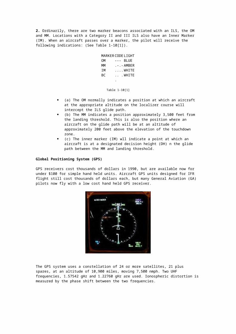
2. Ordinarily, there are two marker beacons associated with an ILS, the OM and MM. Locations with a Category II and III ILS also have an Inner Marker (IM). When an aircraft passes over a marker, the pilot will receive the following indications: (See Table 1-10[1]).

MARKER

CODE

LIGHT

OM --- BLUE MM .-.- AMBE

R IM .... WHIT

E BC .. .. WHIT

E

Table 1-10[1]

(a) The OM normally indicates a position at which an aircraft at the appropriate altitude on the localizer course will intercept the ILS glide path.

(b) The MM indicates a position approximately 3,500 feet from the landing threshold. This is also the position where an aircraft on the glide path will be at an altitude of approximately 200 feet above the elevation of the touchdown zone.

(c) The inner marker (IM) wll indicate a point at which an aircraft is at a designated decision height (DH) n the glide path between the MM and landing threshold.

Global Positioning System (GPS)

GPS receivers cost thousands of dollars in 1990, but are available now for under $100 for simple hand held units. Aircraft GPS units designed for IFR flight still cost thousands of dollars each, but many General Aviation (GA) pilots now fly with a low cost hand held GPS receiver.

The GPS system uses a constellation of 24 or more satellites, 21 plus spares, at an altitude of 10,900 miles, moving 7,500 nmph. Two UHF frequencies, 1.57542 gHz and 1.22760 gHz are used. Ionospheric distortion is measured by the phase shift between the two frequencies.

Two modes are available, the "P", or precise mode, and the "C/A" or Coarse/Acquisition Mode. The P mode used by the military transmits a pseudo-random pattern at a rate of 10,230,000 bits/sec and takes a week to repeat. The C/A code is 10 times slower and

repeats every millisecond.

The GPS receiver synchronizes itself with the satellite code and measures the elapsed time since transmission by comparing the difference between the satellite code and the receiver code. The greater the difference, the greater the time since transmission. Knowing the time and the speed of light/radio, the distance can be calculated.

The timing comes from four atomic clocks on each satellite. The clocks are accurate to within 0.003 seconds per thousand years. The GPS satellites correct for receiver error, by updating the GPS receiver clock. The GPS satellite also transmits its position, its ephemeris, to the GPS receiver so it knows where it is relative to the satellite. Using information from four or more satellites the GPS receiver calculates latitude, longitude, and altitude. (The math involves matrix algebra and the solution of simultaneous equations with four unknowns. Computers do that sort of computation very well.)

GPS receivers provide all needed navigational information including:

Bearing Range Track Ground speed Estimated time en route (ETE) Cross track error Track angle error Desired track Winds & drift angle

Differential GPS or DGPS

DGPS uses a ground station to correct the code received from the satellites for 5 meter accuracy. DGPS could be used for Precision approaches to any airport.

g l o b a l p o s i t i o n i n g s y s t e m s ( G P S )

Navigation is simple - in theory. Determining your position on the surface of the earth requires you to know either your compass bearing to a landmark or the distance separating you from the landmark. Plotting this information on a chart localises your position along a line or arc in relation to the landmark. If you now plot the bearing or distance information of a second landmark, the lines or arcs intersect, and you know that you are located at the intersection point. Simple. Navigators have been using this system for centuries.

The problem with this simple system is that it is not much use if fighting the bar in heavy turbulence with the ATC insisting that you tell you require quick and precise position him where you are, right now. All indication. Getting a compass bearing this, and you don't know where you to a landmark is quick, but not precise. Getting distance information is difficult or impossible - or used to be until a few decades ago. You want to have this information, and be able to plot it, while sitting in a microlight, are on the dinky little map on your knee - Oh boy, do you need GPS!

What are the requirements for a successful position-determining system for you, me and the millions of hikers, 4x4'ers, fishermen and paramedics? Certainly such a system has to be affordable; it also needs to be accurate, easy to use, portable and rugged. Very tough requirements to meet.

Distances between landmarks can be accurately measured by different means. As kids we all used to count the seconds separating the lightning flash and the arrival of the thunderclap. Since we know the speed of sound in air (say 330m/s), we can easily work out the distance between the origin of the flash and the observer. This reasoning of course depends on us seeing the flash at the time that it was generated, which means that we accept that the speed of light is infinite and that there is no delay between the flash being generated and it being observed. In reality, the velocity of light (say 300 000 000 m/s), is high, but it is not infinitely so. If we have an accurate enough timing device, it is possible to determine the time lapse between the generation of a light signal and its reception.

The critical part in this is having a timing device that is accurate enough for the purpose. Using a clock that is accurate to 0,001 second (one millisecond) to determine the time-of flight of a light signal, leads to an error of 300km. Nanosecond accuracy (0,000 000 001 sec) leads to an error of 0,0003km. This 300mm error is much more acceptable, but is totally dependent on the availability of ultra accurate atomic clocks.

As an aside - in 1714 the British Parliament offered a prize of 20 000 pounds to the first person to devise a method of finding longitude at sea with an accuracy of 30 nautical miles. This sum was a great deal of money at the time, but it was claimed only in 1762 by a certain John Harrison, who constructed a clock, the chronometer, that was so accurate that navigators could use it to attain the magic 30 mile precision.

Today we use radio signals instead of pulses of light as the means of determining the distance between a receiver (your GPS equipment and a signal source. Radio signals propagate at the speed of light, and precise distance measurement is possible if very

accurate clocks are available in both the transmitter and the receiver. The signal source needs to radiate a signal containing real time, an identification code and a position indicator. If the signal source were an immovable ground station the positional information would not be necessary. The receiver needs to keep its own accurate time so

that the time-of-flight of the signal can be determined, and it also needs to know from which transmitter (where) the signal originated. Since the US military started with the idea of GPS, they are understandably very concerned about the safety and integrity of ground installations. Another problem with ground stations is that there would need to be a very large number to cover the whole earth. The decision was therefore to go with a satellite system, and the Navstar system was born.

The satellites are big and expensive enough to each contain a few atomic clocks (a few, since there have to be spares and they also need to be checking each other), but your hand - held GPS receiver cannot make use of this bulky and non-affordable timing technology. A timing device that is cheap and small, however, is the ordinary quartz crystal oscillator - the same one that is used in just about all wristwatches. The short term accuracy of such a timing device can be of the order of a microsecond (1 000 nanoseconds), but this is not nearly good enough to allow it to be used directly for computing the distance between the receiver and the satellite. The success of the whole system depends on the implementation of successful strategies to compensate for the receiver clock errors.

Radar Radio Direction And Ranging also makes use of the time that a signal takes to travel between target and antenna, but in this case the process is straightforward. With radar the antenna radiates a strong microwave signal which is bounced off the target and which is then reflected back to the antenna. The process involves the determination of the time-of-flight of the signal, dividing this value by two and then computing the distance. Here the interval between sending and receiving a signal is determined by the sender - accurate real-time clocks are not necessary at all. Trivial, compared to the requirements for GPS.

Having more than one satellite available in the sky allows your GPS receiver to compute the distance between itself and various 'visible' satellites. Determining the distances to more than two satellites allows you to plot your position accurately. Since each distance plot places you somewhere on the surface of a sphere centered on a satellite, using data from three satellites allows the position of the receiver to be calculated to being within a three-sided volume of space. The size of this volume depends on the accuracy of the data, and therefore primarily on the accuracy of the clocks. The microsecond accuracy of the receiver clock does not lead to acceptable volume sizes.

Solving the clock error problem is crucial. Determining a position on earth requires values for three unknowns; x, y and z-positions. We know from high school algebra that solving for three unknowns requires at least three independent equations. Three satellites will give us x, y and z, but imprecisely, since we do not know the value of a fourth variable, which is the time error of the GPS receiver. This means that we have an equation with four unknowns: x, y, z and the time error. Getting information from a fourth satellite makes it possible to solve for this fourth unknown. The GPS receiver makes use of an iterative, or repetitive, mathematical algorithm to determine the time error.

This value is then used to re-compute distances to all four (or more) satellites. As a bonus, in addition to the positional information, the GPS system therefore provides time signals accurate to within about 200 nanoseconds. This then also is

the reason why the time readout of a GPS-receiver cannot be re-set by the user - it is continually being computed from the information received from at least three independent atomic clocks, and this is why it always extremely accurate. If your GPS time readout differs from that given by the SABC, the SABC is wrong and you are right!

Signals from four satellites provide 3D (x, y and z) and time information. Three satellites lead to 2D information - x, y and time, while the z or altitude information cannot be computed.

The above description makes all this sound rather easy. If the satellites were fixed in space it would in actual fact be so. But, the satellites are not fixed in space. They circle the earth at 14000 km/h at a distance of 20 190 km, in orbits that take 11 hours 58 minutes to complete, so that they seem to drift, like the stars, four minutes per day. In contrast to this, geostationary satellites (like many communications satellites), are at 36 000 km from the earth and circle the earth once in exactly 24 hours so that they always stay over the same spot on the surface of the earth. Geostationary satellites have one attribute that makes them unsuitable for GPS-use, and that is the fact that they can only be launched into equatorial orbits, which would give very poor visibility from high and low latitudes. It would also mean that they are all in the same plane, making for very poor positional accuracy.

To give good coverage to GPS receivers anywhere on earth, there are always at least 24 satellites (or Space Vehicles, SV's, as they are often referred to) in orbit. Of these, three are spares. Four SV's travel in each of six orbits, each inclined at 55° to the equator so that four or more of the SV's are at all times visible from any point on the surface of the earth. In addition to the atomic clocks and the communications equipment each satellite also contains fuel for its small manoeuvring engines, giving it a limited capability of orbit adjustment.

In addition to the Navstar satellites in space (the 'Space Component'), there is also a ground support system (the 'Control Segment') with a master control station and a number of monitoring stations around the world. The last component of the system is the 'User Segment', which includes us with our GPS receivers.

Once a SV is in space, it does not stay in exactly the same orbit from day to day. There are factors that influence the orbit unpredictably, such as pressure from the solar wind, and predictably, like the gravitational effects of the moon and planets. The ground stations of the Control Segment need to determine the speed and position of each satellite with great accuracy so that it can predict and describe the satellite's orbit unambiguously. Such a description of the satellite clock parameters and its orbital characteristics is called an ephemeris, and this information is uploaded to each individual satellite. The ephemeris information can be updated twice per day as the satellite passes over a ground station. When or if the ground station finds that a satellite has wandered from its predicted position in orbit, the orbit is re-computed and the data uploaded to the satellite. Since there is limited fuel on board, it is only as a last resort that the satellite is physically moved with the aid of its own engines. This happens when the orbit deviates so much from the desired path that accurate prediction is no longer possible. When your GPS receiver acquires information from a satellite, the ephemeris data is received, and this is what allows

it to measure the time difference between when the signal was broadcast and when it was acquired, so that it is possible to compute the distance between satellite and receiver.

All the satellites broadcast information continuously on the same two frequencies, the L1 frequency at 1575.42MHz, and L2 at 1227.6MHz. Cost and bulk considerations cause most or all small receivers to utilise only the L1 frequency. The radiated power of a satellite transmission is not much more than 500W. Compare this with the radio in your microlight, putting out 5W. The difference being that the satellite is at least 20 000 km distant, and if it appears to be low on the horizon, it is much further away than this. The signal arriving at your receiver is therefore barely distinguishable above the background electronic noise.

The small non-directional antenna on the GPS receiver recovers this extremely low level, noisy signal) and passes it to the receiver where spread spectrum technology deciphers the signal. The advantage of spread-spectrum is that it can extract a very low-level signal from background noise, but it can only do so at the expense of speed. Data rates of 50 bits per second are the norm. If a receiver needs to acquire all the information that a satellite broadcasts, which includes ephemeris data and 'almanac' data, the process will take more than 1 0 minutes to complete. Normally the receiver only needs the ephemeris information from the satellite.

So, what influences the signal during the transit between satellite and GPS receiver?

The distance between the satellite and the receiver.  

The relativistic effect of the satellite moving relative to the earth. Einstein demonstrated that time is retarded when velocity increases. Even though the satellites move at a low fraction of light speed, nanosecond accuracy implies that correction is needed for the relativistic effects of satellites either approaching or receding from the receiver.

The rotation of the earth under the satellite displaces the receiver during the time-of-flight of the signal.  

Doppler-shift - this being a function of the rate at which the satellite approaches or recedes from the receiver. This changes the frequency of the received signal in the same way that the frequency of the noise of an approaching vehicle seems to be high, and suddenly becomes lower when the vehicle passes the observer. This doppler-shift is used by the GPS system to determine your speed and the direction that you are moving in. If the satellites were in geo-stationary orbits, this information would not have been available. The TRANSIT satellite system, used by the US Navy, is (was) an earlier-generation positioning system using primarily doppler-shift for determining position. This is not really useful for rapidly moving receivers, since the receiver movement influences the observed doppler-shift and reduces accuracy.

Precession of the earth's rotation axis. The wobble of the axis takes more than 25 000 years to go through a complete rotation, but it is also corrected for in the computation.

The refraction of the radio signals by the ionosphere and the troposphere. Since these layers are inhabited by charged particles, they have an influence on the propagation of the signals The path of the signal through the layers are lengthened or shortened, depending on the apparent angle of the satellite above the horizon. The effect on the signal can be determined by measuring the difference in scattering between the L1 and L2 frequencies. This can then be accurately corrected for. This is what is done in dual-frequency receivers, but in our small single- frequency consumer systems a mathematical algorithm adequately, if not perfectly, corrects for the effect.

This process can take many minutes, even tens of minutes. The same thing may happen if you do not use the unit for some months, and the receiver considers the almanac data to be out of date If the receiver has valid almanac data, it 'knows' which satellites to expect, and where they are located at that specific time. Determining the doppler frequency of the signal is the next step. This is done by listening at each of 20 or to predefined frequencies close to L1, and measuring signal strength at each. This is speeded up by the receiver being able to compute the expected frequencies by using the satellite locations kept in memory, by correcting for its own oscillator error based on previous error values also kept in memory, and predicting its own oscillator frequency based on the current temperature.

Once it has determined the frequency for each satellite it starts to receive data on the L1 frequency. The satellites nearest to the overhead position are preferred for initial acquisition. Each satellite broadcasts its own identification code in the form of a 1023-bit pseudo-random number sequence, repeated every millisecond.

The receiver needs to set its own clock to the correct time slot. It does this by trying all the possible values. This process may take one or two seconds. In many GPS receivers this stage of the proceedings is shown on the display by the satellite acquisition histogram bar becoming visible as a hollow bar.

As soon as it has locked onto and identified a satellite, the downloading of ephemeris data can start. There is approximately 1 500 bits of data in a message and this is sent at 50bps. This download takes about 30 seconds. This needs to be done for at least three satellites to be able to compute x, y and time. If more satellites are in range, data are acquired from them as well. The downloading can be done via more than one channel, and can also be multiplexed amongst the satellites, so that the process need not take more than a minute or so. The successful downloading of ephemeris data for a specific satellite is often indicated on a GPS receiver by the hollow histogram bar turning solid black.

If the receiver is switched on within a few minutes of a previous session, it will get a fix on its position in usually less than 20 seconds. This can happen since it saves the ephemeris

data that it held at its previous shutdown. Under these circumstances it will verify that the ephemeris data is still valid and that the relevant satellites are still 'visible'.

Ephemeris data from a satellite is considered to be valid for four hours (the transit time from horizon to horizon), but is in any case updated after two hours. Once this downloading is done, the CPU in the receiver can get to work and determine the position of the receiver. To do this it performs a variety of computational steps.

The dedicated central processing unit in the receiver translates the ephemeris data into a format suitable for its calculations.   It calculates the satellite positions so that it has accurate elevation and bearing

parameters to base its troposphere modelling on.  It calculates initial distances (pseudo-range) on which ionosphere modelling is based.   These steps are repeated for each satellite in range.   It corrects for the earth's rotation, based on the pseudo-range data.   Recalculates the receiver position.   Corrects the altitude data for geoid height. Displays the position on the receiver readout. Corrects the time signal for UTC offset and other factors and displays it. Continually recalculates the position based on the data from additional (more than four)

satellites and displays the best possible solution.   Calculates horizontal speed by using the Doppler information. The result of all this is a

position in latitude and longitude, altitude, time and horizontal speed. The accuracy of these values depends on two factors. The inherent limitations of dock accuracy and parameter modelling.

  The factor called Selective Availability (SA). There has always been concern that the Navstar system can be used for military purposes against the US The system is under control of the US Department of Defence, but the non-military use was deemed to be so important that the decision was taken to make the system available for civilian use, but with reduced accuracy.

To this end they introduced a random degradation of the accuracy of the data. Since this is a random degradation, the accuracy is not always the same. Sometimes there is no degradation, at other times there may be a maximum degradation - there is no way to know what the effect is. The result is that the accuracy can only be expressed statistically, and the official description is: Horizontal (long-lat) - within 100m for 95% of the time, and within 300m 99.99% of the time. Vertical (altitude) - within 1 56m for 95% of the time, and within 100m 99.99% of the time.

In practice the values are appreciably better than this. Various measurements, under different conditions,' have been made over the years. Results have shown that average horizontal accuracy have tended to be around 50m.

Human nature being what it is, there has been a great deal of indignation over this degradation of a perfectly good signal. Various methods have been used to improve accuracy. One of the most widely used depends on the presence of ground stations transmitting very accurate time signals from very accurately known positions. The user buys an additional receiver for this signal and feeds in this "Differential" signal into the GPS receiver.

This very accurately corrects for the clock error and the introduced SA and allows average horizontal accuracy of 1 to 4m and altitude averages of less than 10m. These DGPS values have been widely used for accurate navigation and surveying.

V O R n a v i g a t i o nour thanks www.raa.asn.au (Copyright John Brandon)

VOR transmitter

general

VHF Omni-directional Radio Ranges [VORs] operate in the Very High Frequency aviation navigation [NAV] band between 112.1 and 117.9 MHz. As VHF transmissions are line-of-sight the ground to air range depends on the elevation of the beacon site, the height of the aircraft and the power output. The VOR beacons are usually located at airfields but as they serve to define designated air routes [ airways] some are located away from airfields, often on high ground.

A simplified concept of the ground beacon is that it simultaneously transmits two signals, a constant omni-directional signal called the reference phase and a directional signal which rotates through 360°, during a 0.03 second system cycle, and consistently varies in phase through each rotation. The two signals are only exactly in phase once during each rotation – when the directional signal is aligned to magnetic north.

Imagine a wheel with 360 spokes, at one degree azimuth spacing, with the VOR beacon being the hub. The spokes are numbered clockwise from one to 360 and each spoke or radial represents a magnetic bearing from the VOR beacon. The airborne navigation circuitry measures the phase angle difference between the directional signal phase received and the reference signal phase and interprets that as the angular, or 'radial', indication currently being received. Radials are identified by magnetic bearing – e.g. the 30° radial – and thus form the basis for VOR, and designated air route, navigation. Essentially the system indicates a line of position, from the selected VOR, on which the aircraft is located at any time.

The beacon also transmits a Morse code aural identification signal at about 10 second intervals.

The airborne system utilising the VOR beacon transmissions usually consists of an antenna (probably a V - type dipole mounted horizontally on the fin or fuselage but could be the

more expensive 'blade' or 'towel rail' types), a conventional VHF receiver (if combined with the VHF communications transceiver it is then called a NAV / COMM unit), navigation circuitry and the separate panel mounted navigation indicator or 'Omni Bearing Indicator' [OBI].

Some hand held aviation COMMS transceivers can also receive the NAV band VOR transmissions and appear to have some navigation circuitry but, from all reports, their VOR navigation capability, if it exists at all, is limited.

Basic Omni Bearing Indicator, like this Bendix-King model, has a manually operated radial or 'omni bearing' selector [OBS] which rotates an azimuth ring marked from 0° to 355°. The OBS selected radial is indicated by the arrow at top dead centre and the reciprocal bearing is indicated by the bottom arrow. The other features of a basic OBI are the TO–FROM indicators, a deviation bar, a deviation indicator needle and a NAV/OFF alarm flag.

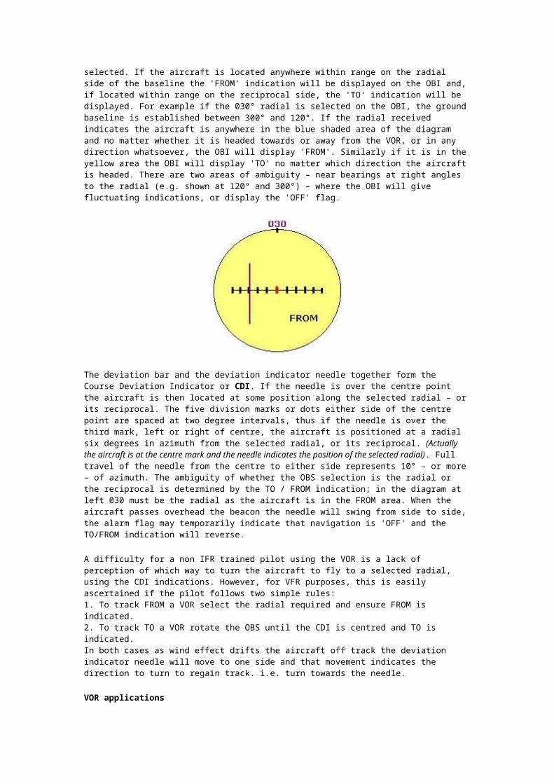
The TO–FROM indications on the OBI are dependent on the aircraft's position relative to a notional ground baseline, formed perpendicular to the selected radial and passing through the beacon site. Unlike the NDB the indication is completely independent of the aircraft's heading. The navigation circuitry compares the difference between the radial being received and the radial selected. If the aircraft is located anywhere within range on the radial side of the baseline the 'FROM' indication will be displayed on the OBI and, if located within range on the reciprocal side, the 'TO' indication will be displayed. For example if the 030° radial is selected on the OBI, the ground baseline is established between 300° and 120°. If the radial received indicates the aircraft is anywhere in the blue shaded area of the diagram and no matter whether it is headed towards or away from the VOR, or in any direction whatsoever, the OBI will display 'FROM'. Similarly if it is in the yellow area the OBI will display 'TO' no matter which direction the aircraft is headed. There are two areas of ambiguity – near bearings at right angles to the radial (e.g. shown at 120° and 300°) – where the OBI will give fluctuating indications, or display the 'OFF' flag.

The deviation bar and the deviation indicator needle together form the Course Deviation Indicator or CDI. If the needle is over the centre point the aircraft is then located at some position along the selected radial – or its reciprocal. The five division marks or dots either side of the centre point are spaced at two degree intervals, thus if the needle is over the third mark, left or right of centre, the aircraft is positioned at a radial six degrees in azimuth from the selected radial, or its reciprocal. (Actually the aircraft is at the centre mark and the needle indicates the position of the selected radial). Full travel of the needle from the centre to either side represents 10° – or more – of azimuth. The ambiguity of whether the OBS selection is the radial or the reciprocal is determined by the TO / FROM indication; in the diagram at left 030 must be the radial as the aircraft is in the FROM area. When the aircraft passes overhead the beacon the needle will swing from side to side, the alarm flag may temporarily indicate that navigation is 'OFF' and the TO/FROM indication will reverse.

A difficulty for a non IFR trained pilot using the VOR is a lack of perception of which way to turn the aircraft to fly to a selected radial, using the CDI indications. However, for VFR purposes, this is easily ascertained if the pilot follows two simple rules: 1. To track FROM a VOR select the radial required and ensure FROM is indicated. 2. To track TO a VOR rotate the OBS until the CDI is centred and TO is indicated. In both cases as wind effect drifts the aircraft off track the deviation indicator needle will move to one side and that movement indicates the direction to turn to regain track. i.e. turn towards the needle.

VOR applications

Like the NDB / ADF there are several applications for the VOR in light aircraft cross country VMC navigation. The applications briefly described below will be detailed in the 'Using the VOR' module.

Homing & tracking to a VOR. Even with a crosswind component tracking toward a VOR is quite simple, rotate the OBS until the CDI is centred and TO is indicated, turn onto that magnetic heading and then just keep the CDI centred and you will track more or less direct to the VOR.

Tracking from a VOR. Rotate the OBS to the required track [radial], ensure FROM is indicated, turn onto that magnetic heading and just keep the CDI centred and you will maintain the track.

Position fixes. If two VORs are in range then the bearing from each can be ascertained, roughly plotted on the chart [after converting to true bearings] and the aircraft position will be close to the intersection point of the LOPs. Alternatively a VOR bearing and a NDB bearing can be used or a VOR bearing and a line feature on the chart, the latter technique being the most frequently used.

Running fix / distance from VOR. The 1-in-60 rule can be applied when the aircraft is within range of a transmitter by turning the aircraft so that the station is abeam and then measuring the degrees traversed against time, as in the NDB running fix application above. The advantage with the VOR is that the CDI needle indicates the degrees traversed. As in the NDB application the position fix is the distance along the second radial from the beacon.

VOR errors

Standard VOR systems are more accurate than NDB / ADF but are still subject to errors at the ground station, bending distortion of signals caused by terrain effect and avionics errors. The aggregation of all errors is very unlikely to exceed 5°.

Though very thin on the ground in the outback areas of Australia, NDB and VOR can be very useful, provided the aircraft is within range, but not the best value for money. That distinction now belongs to another, and more advanced, supplementary navigation tool – the Global Positioning System.

Navigating directly to a VOR is the easiest way to use this kind of navaid.

Dial in the frequency of the VOR into your NAV1 radio Turn the OBS (course selector knob) for the instrument(OBI) until you see the word

"TO" and the CDI needle centres Note the heading shown at the top of the instrument; fly that course to go directly

to the VOR

That's basically all there is to it! There are complications such as crosswinds that will affect your ability to get to the VOR. If you have winds you will have to adjust for them and fly a heading that will allow you to follow the proper course.

In an ideal situation you could fly the heading you just determined right to the VOR station. In that case the needle on the OBI would remain centred right up until the time when you passed over the VOR. More likely, though, your course will drift off to the side. By watching the needle on the OBI you can see this happen and also tell how to adjust your heading to get back on course:

try this excellent programme by Tim Carlson

Your browser does not support inline frames or is currently configured not to display inline frames.

Control Function

MouseClick/

Drag on the Map

Move the airplane, the transmitters, or change the wind vector (if in wind mode)

  Click the Buttons Change the vector (OBS) for the instrument (except the RMI, DG)

Keyboard

Up & Down

ArrowsIncrease or decrease the airplane speed (60-300 kt - my future Lancair IVP)

 Left and

Right Arrows

Increase or decrease turn rate (deg/sec)

  Space Bar Instantly set the turn rate to zero

  Enter Reposition transmitters to original positions - useful if you've moved them off the map

  R Toggle radials on & off (dark colours = from side of VORs, light colours = TO side of VORs)

  1 or 2 Switch instrument 1 or 2 between VOR, HSI, ADF, RMI, DG, or Text

  W Toggle Wind mode (shown in status line) - when in wind mode you can click/drag on the map to change the wind vector

  P Pause the animation (wind and airplane motion) - you can still rotate the instruments and drag the plane

  T Trace - start/stop a trail of dots showing the airplane's path

  H Hide - stop/start displaying the airplane and trace  L Lost - randomly reposition the airplane on the map - most useful when

the plane is hiddena u t o m a t i c d i r e c t i o n fi n d e r ( A D F )

Some aircraft are equipped with an ADF receiver. They receive radio signals in the medium frequency band of 190 Khz to 1750 Khz. The ADF receiver can “Home” on both AM radio stations and Non-Directional Beacons. Commercial AM radio stations broadcast on 540 to 1620 Khz. Non-Directional Beacons (NDBs) operate in the frequency band of 190 to 535 Khz.

The aircraft equipment consists of two antennas, the ADF Receiver, and the ADF Instrument. The two antennas are called the (1) LOOP antenna and the (2) SENSE antenna.

The loop antenna can sense the direction of the signal from the station, but cannot discriminate whether the station is in front or behind the aircraft. The sense antenna can discriminate direction, and solves the ambiguity of the loop antenna.

The receiver unit has tuning dials to select the station frequency A volume control allows the audible volume to be controlled for identifying the station. The volume can be reduced to prevent interference with other communications. You should, however, continuously monitor the identifier while using the NDB for navigation.

The navigational display contains a compass rose dial graduated in 5 degree increments from 0° to 355°, a pointer with an arrow on one end, and a square form on the other end. We will call the arrow end the “Pointer”, and the square end the “Tail” for the sake of identification.

There are 2 types of compass rose dials that can exist in the navigational unit. One is a fixed compass rose, called a “Fixed Card” ADF. Zero degrees is always shown on top of the card. The “Rotateable Card” ADF allows the compass rose card to be rotated. Interpretation of these displays will be more fully described in later paragraphs.

Non-Directional Beacon (NDB)

Non-Directional Beacons are depicted on aeronautical charts as a circular band of magenta coloured dots. A rectangular magenta box near the NDB symbol shows the name of the station, the 2 or 3 letter identifier, and the Morse code transmitted by the station.

NDBs may be located on the surface of airports, or may be within a few miles from an airport. Sometimes they are co-located with the Outer Marker in ILS approaches. The NDB provides two principal functions; (1) homing for VFR operations, and (2) ADF instrument approach capability for IFR operations.

Because the frequency is below and within the commercial AM band, reception is subject to the same atmospheric disturbances as AM radio, in particular, noise generated by lightening.

ADF Orientation

The pointer end of the ADF navigation unit ALWAYS POINTS TO THE STATION. The degree reading on the display is dependent on the aircraft heading. In the diagram if the heading of the aircraft changes, the arrow will always point to the station and the degree reading on the instrument which the pointer indicates also changes..

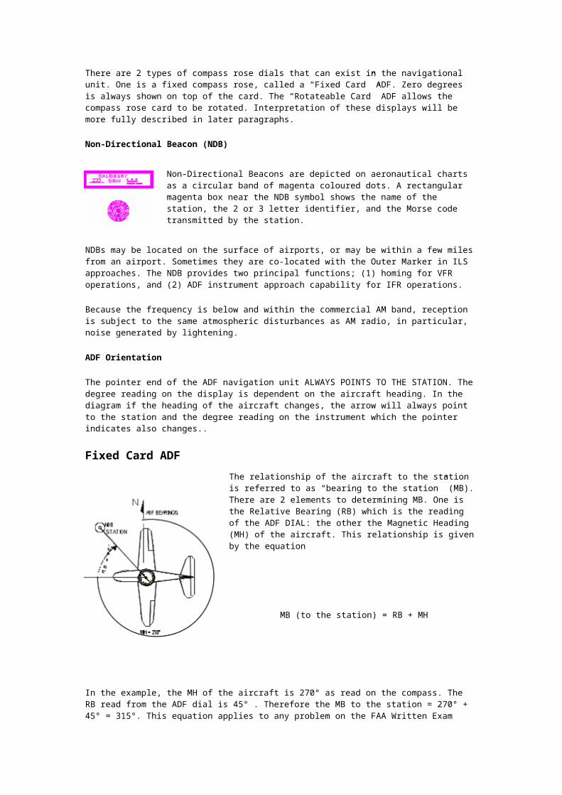
Fixed Card ADFThe relationship of the aircraft to the station is referred to as “bearing to the station” (MB). There are 2 elements to determining MB. One is the Relative Bearing (RB) which is the reading of the ADF DIAL: the other the Magnetic Heading (MH) of the aircraft. This relationship is given by the equation 

 MB (to the station) = RB + MH

 

 

In the example, the MH of the aircraft is 270° as read on the compass. The RB read from the ADF dial is 45° . Therefore the MB to the station = 270° + 45° = 315°. This equation applies to any problem on the FAA Written Exam relating to the Fixed Card ADF. If any two values are known, the third can be computed.

Moveable Card ADF

Some aircraft are equipped with an ADF instrument in which the dial face of the instrument can be rotated by a knob. This is called a Moveable Card ADF. By rotating the card such that the Magnetic Heading (MH) of the aircraft is adjusted to be under the pointer at the top of the card, the Bearing to the Station (MB) can be read directly from the compass card. More sophisticated instruments of later design automatically rotate the compass card

of the instrument to agree with the magnetic heading of the aircraft. Thus MB to the station can be read at any time without manually rotating the compass card on the ADF face.

Tracking to an NDB

A useful ADF application in visual navigation is to locate a particular NDB and then track – or home – directly to it. The ADF receiver is tuned to the NDB frequency, and the audio volume turned up, so that the NDB can be identified as soon as the aircraft comes within range. The ADF needle indicates the bearing to the NDB and the wind correction angle necessary to maintain that track is then ascertained by bracketing, a technique which bears some similarity to the double track error method. The term 'bracketing' is derived from the artillery technique for ranging the target by deliberately placing initial rounds behind and in front of it.

Note: this sequence is best performed if the heading being flown is positioned on the ADF card at TDC, the diagrams in the left column below indicate the readings with those settings.

 

procedure

Needle position Compass heading Event sequence

060°

Position A. When receiving the NDB signal turn the aircraft so that the head of the ADF needle is pointing to TDC, then check the heading from the compass. That heading is the track required to home directly to the NDB, for our example 060° magnetic. Rotate the ADF compass card to set 060° at TDC and the needle head will also indicate 060°. Remember that all heading changes should be logged.

060°Position B. As the flight progresses, holding the 060° heading, the crosswind causes the aircraft to drift to the south of the required track and the ADF needle has moved left about 5° to 055°.

030°

Position C. We now have to make a first rough cut at the track error – it is best to initially overestimate so let's choose 15° and, applying the double track error technique, we turn left 30° on to an intercept heading of 030° magnetic. Positioning the 030° heading at TDC, the head of the needle will still initially indicate 055° but will move towards 060° as we close with the required track.

045°

Position D. When the needle reaches 060° the 060° track to the NDB has been regained. Now halve the intercept angle (i.e. subtract the track error) and turn right onto an initial wind correction heading of 045° magnetic, i.e. the estimated track error was 15°, we turned left 30° onto the intercept heading of 030° and now, having regained the required track, we turn right 15° onto a wind correction heading of 045°.

Now rotate the card to the 045° heading and the needle remains at the 060° bearing.

045°

Position E. If the 15° WCA is correct then the ADF needle will remain at the 015° position whilst the 045° heading is maintained. However it is most likely that we have overcorrected, the aircraft will drift north of track, shown by the needle moving clockwise a few degrees from the 015° position so we now have to refine the wind correction angle.

055°

Position F. We might guess that we have overestimated the WCA by about 5° so, applying the double track error technique, we turn right 10° on to an intercept heading of 055° magnetic. Positioning the 055° heading at TDC, the head of the needle will still initially indicate something greater than 060°, say 063°, but will move towards 060° as we close with the required track.

050°

Position G. When the needle reaches 060° the 060° track to the NDB has been regained. Now halve the intercept angle and turn 5° left onto a wind correction heading of 050° magnetic, rotate the card to the 050° heading and, if we've estimated correctly, the needle will remain at the 060° bearing, maintaining a 10° WCA, while we continue along the required 060° track to the NDB.

Tracking from an NDB

Another useful application for the ADF in visual navigation is in determining track error when departing from an airfield equipped with an NDB or when overflying an NDB.

For example: the flight plan calls for a departure – from overhead an NDB – on a track of 240° magnetic with any necessary wind correction to be assessed after departure – using the ADF – with the track recovery and heading correction to be made by a slightly modified double track error method. (The modification is that rather than timing the intercept leg to estimate track recovery we will use the ADF needle to indicate when we are back over the required track.)

In this ADF application the ADF card may be used with the 0° position set at TDC or your personal preference may be to set the 240° heading at TDC. The diagrams and the text below indicate the procedure and the readings with 0° positioned at TDC but the additional text in italics is the procedure when rotating the card to the new heading for every change. Hopefully you will be able to see that the latter method is easier to handle.

Note that when tracking away from an NDB we use the tail of the ADF needle, rather than the head, as the indicator.

 

 

Needle position Compass heading Event sequence

240°

Departing from overhead the NDB to track 240° magnetic.

The magnetic compass heading is 240° ( i.e. no wind correction provision) and the tail of the ADF needle swings to the 0° position.

With the 240° magnetic heading set at TDC the position of the needle relative to TDC is exactly the same as in the diagram but, on the background card, the needle tail indicates the 240° heading.

240°

Position B. As the flight progresses holding the 240° heading the crosswind causes the aircraft to drift to the south of the required track.

The tail of the ADF needle has moved about 15° to 345° and is in the left half of the card. Thus the opening angle, or track error, is 15° and the tail of the needle represents the track made good, which is 15° to the left of the required track.

With the 240° magnetic heading set at TDC the tail of the needle will indicate the track made good, 225° or an opening angle, or track error, of 15°.

270°

Position C. Use the double track error method to intercept the required track.

The aircraft is turned 30° [2 × 15] onto a heading of 270° magnetic. The ADF needle tail initially moves 30° to 315° then commences to reverse direction as the 270° heading is maintained and the aircraft is closing the 240° track out.

The aircraft is turned 30° [2 × 15] onto a heading of 270° magnetic and 270° magnetic is now set at TDC, the tail of the needle will then initially still indicate 225° but will move towards 240° as you close with the required track.

270°

Position D. When the needle has moved through a 15° arc and is back to the 30° left position [330°], on a heading of 270°, the 240° track out from the NDB has been regained.

With the 270° magnetic heading set at TDC the 240° track out from the NDB has been regained when the tail of the needle reaches 240°.

255°

Position E. Subtract the track error [15°] and turn left onto the new heading of 255° which will then maintain the necessary 15° wind correction angle.

The ADF needle moves 15° clockwise and the aircraft should hold the required track – if the heading is maintained and the needle kept at the 345° position.

Subtract the track error [15°] and turn left onto the new heading of 255° which will then maintain the necessary 15° wind correction angle. Set the 255° magnetic heading at TDC, the tail of the needle now indicates 255°.

After flying this heading for a while you may find that you still have some drift – indicated by movement of the needle. In this case a small heading correction is usually enough compensation.

Running fix / distance from NDB

Whenever your track will pass abeam an NDB it is quite easy to obtain a running fix, using the 1-in-60 rule and a little mental arithmetic, providing you have a reasonable idea of your groundspeed. The technique is illustrated in the diagram:

Procedure

1. Tune and identify the NDB, set your heading at TDC and watch the ADF needle, the NDB is directly abeam when it moves to 90° either side of TDC, position A in the diagram.

2. Note the time and continue flying your heading, for example 040° magnetic.

3. When the needle has moved a sufficient amount to get a good reading (position B on the diagram), note the time and the bearing from the NDB, indicated by the tail of the needle. Let's say the needle has moved 10°, the elapsed time is 8 minutes, the bearing from the NDB is 110° magnetic and you reckon your groundspeed at 70 knots.

4. Now we calculate the distance we are along that bearing using the 1-in-60 rule: i.e the distance [nm] from the NDB = elapsed time [minutes] × ground speed [knots] / degrees traversed = 8 × 70/10 = 56 nm. The aircraft's position at time B is then 110°/56 nm from the NDB. The real difficulty now is to measure and plot that position on the navigation chart whilst flying the aircraft (not forgetting to convert the bearing to °true) – so best to get the passenger to do it.

If you are wondering what happened to the '60' in the 1-in-60 application the answer is it is negated by the usage of minutes in one factor and nautical miles per hour in another. In the diagram the dashed red line outlines the right angle triangle on which the calculation is based – the distance from the NDB to position B forms the hypotenuse.

ADF applications

There are several applications for the ADF in light aircraft cross country VMC navigation – remembering the Visual Flight Rules require that the pilot must be able to navigate by reference to the ground and position fixes must be taken at least every 30 minutes.

Position fixes. If two (or better - three) transmitters are in range then the bearing from each can be ascertained, the lines of position roughly plotted on the chart (after converting to true bearings) and the aircraft position will be close to the intersection point. In most of Australia to have two NDBs in range at the same time is not so common and three would be most unlikely, so the most likely position fixing use is to combine a surface line feature with an NDB bearing.

Running fix / distance from NDB. The 1-in-60 rule can be applied when the aircraft is within range of a transmitter by turning the aircraft so that the station is abeam and then measuring the degrees traversed against time. This is a form of running fix in that two bearings are taken, at an interval, from one source and the aircraft's position is the distance along the second LOP from the NDB. For example:

Distance [nm] to NDB = elapsed time [minutes] × ground speed [knots] / degrees traversed

Homing & tracking to or from an NDB. If there is no crosswind component then tracking toward an NDB is quite simple, just keep the head of the ADF needle at TDC and you will arrive overhead; the track over the ground will be straight and the magnetic heading consistent. However if there is a crosswind component and you just endeavour to keep the head of the ADF needle at TDC, you will eventually arrive but, due to the drift, the track followed will be curved and the magnetic heading will need to be consistently changing. This is called homing, and you will arrive at the NDB on an into-wind heading. Thus tracking, or flying directly towards, or from, an NDB is exactly the same as tracking from A to B – you have to calculate a wind correction angle. Passage overhead an NDB is signified by a "cone of silence" (if the ident volume has been turned up beforehand) and the needle then swinging to the reciprocal bearing.

Using the ADF probably appears to be fairly simple, which it is, but there will be difficulties, for the uninitiated in perceiving, from the position of the needle, the headings to fly when attempting to intercept and then track along a particular magnetic bearing to or from the ground station.

As in all navigation you should always maintain an awareness of the aircraft's position in terms of being north, south, east or west of the NDB and, when initiating a turn, think in the same terms e.g. a left turn will take you further east.

NDB/ADF errors

Electrical interference. Radio waves are emitted by the aircraft alternator in the frequency band of the ADF. An alternator suppressor is fitted to contain those emissions but this

component does not have a long life and it is wise to test the ADF for correct operation during pre-flight checks. The test is made by selecting a transmitter – which must be a reasonable distance away, say 30 nm – then watch the ADF needle during the engine run up. If the needle moves as rpm increase there is electrical interference and probably the alternator suppressor should be replaced. Magnetos may also interfere with the ADF.

Thunderstorms emit electrical energy in the NDB band and will deflect the ADF needle towards the storm.

Twilight/night effect. Radio waves arriving at a receiver come both directly from the transmitter – the ground wave – and indirectly as a wave reflected from the ionosphere – the sky wave. The sky wave is affected by the daily changes in the ionosphere, read the ionisation layers section in the Aviation Meteorology Guide. Twilight effect is minimal on transmissions at frequencies below 350 kHz.

Terrain and coastal effects. In mountainous areas NDB signals may be reflected by the terrain which can cause the bearing indications to fluctuate. Some NDBs located in conditions where mountain effect is troublesome transmit at the higher frequency of 1655 kHz. Ground waves are refracted when passing across coast lines at low angles and this will affect the indicated bearing for an aircraft tracking to seaward and following the shore line.

Attitude effects. The indicated bearing will not be accurate whilst the aircraft is banked.

t r a c k e r r o r a d j u s t m e n t s

The track plot below shows the first leg of our planned flight between Oxford and Tottenham. The green lines are the 10° drift lines and the pink marks along the track are the 10 nm distance marks. In this example the first three marks are distance from Oxford, the last three are distance from Warraway Mountain, and the longer mark is the track midpoint. For the colour blind amongst us the track is orange.

Instead of distance marks some navigators favour time marks at, say, 10 minute intervals. However time marks really don't co-relate that well with charts – time notations are more properly confined to the log.

As it is remarkably easy to set off in the wrong direction – reversed application of variation for instance – it is advisable to note a landmark as a means of verifying that, at the set course point, you really are setting off along the required track. The sun's position provides a gross indication of heading which will at least confirm that you are not flying the reciprocal course. Starting off in the wrong direction, without realisation, really makes progress monitoring difficult when you are flying over relatively featureless terrain. In addition a position fix must be acquired within 15 to 20 minutes of the set heading time.

At any time after departure, when the aircraft's position has been pinpointed and found to be off track, heading adjustments will be necessary: initially to regain the required track and then to maintain it or, alternatively, for a new heading to track directly to the next

turning point. There are several methods for calculating and applying heading adjustments – and I suggest you may now find pencil and paper handy.

Double track error method

This is the recommended method if the position fix shows the aircraft to be less than halfway along the leg – hence the reason for marking that midpoint on the chart. The procedure is as follows:

      1.   Using the diverging 10° drift lines estimate the track error – the difference in degrees between the track required and the track made good. The track error is also referred to as the opening angle or sometimes as the drift angle. (The term 'drift angle' in this context is deprecated as it normally refers to the angular difference between the heading flown and the track made good.)

For example let's say, on our Oxford to Warraway Mountain segment, we find ourselves crossing the railway line at Trida and estimate the track error as 6° north of required track. i.e. the track made good is 077° magnetic. We log the time and note 24 minutes have lapsed since departing the set-course point.

      2.   Double the track error and add or subtract that value from the planned heading to arrive at the heading to regain track or the intercept. If the drift was to the right of track the new heading must be to the left of the original heading and, conversely, if drift was to the left the new heading must be to the right of the old. The time we must remain on this new heading, until intercepting the required track, is roughly equivalent to the time flown on the original heading.

Although we have used the terms 'left' and 'right' you will find it more helpful, when considering position, to think in terms of 'north', 'south', south-west' etc.

For example track error is 6° north [left] and original heading 079° magnetic, thus the heading to regain track is 079 plus 12 = 091° magnetic [096° compass] and we fly that for 24 minutes – the same time as that flown on the original heading.

      3.  After it is visually evident that the required track has been reached, or the required time has passed, subtract the track error and turn onto the new heading to maintain the required track and log the event.

For example the track error was 6° and the heading to regain track is 091° magnetic, thus the heading to maintain track is 091 minus 6 = 085° magnetic [090° compass] and we fly that until either a new position fix is obtained or we reach the waypoint.

Theoretically this method doesn't work if the position fix is past the halfway point because the point at which the required track is finally regained would be past the waypoint.

Track error/closing angle method

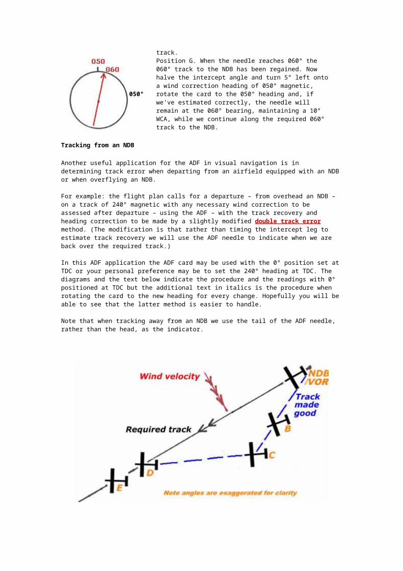
The recommended method if the position fix shows the aircraft to be more than halfway along the leg, or if you choose to fly directly to the waypoint at any time, is as follows:-

      1.   Using the diverging 10° drift lines estimate the track error or opening angle – the difference in degrees between the track required and the track made good. Then using the converging drift lines estimate the direct track to the waypoint and the angle between that track (the new required track) and the original required track. This is usually called the closing angle.

For example let's say, on our Oxford to Warraway Mountain segment, we fix our position as one mile south of the Dundooboo Ridge with an estimated track error of 7° north of required track and the closing angle to the waypoint is about 9°.

      2.   Add the track error and closing angle and apply the value as a correction to the original heading. If the drift was to the left of the required track the new heading will be to the right and vice versa.

For example 7 plus 9 is 16°, drift was to the left of the original heading 079° magnetic, thus the heading – to track directly to the waypoint – is 095° magnetic [100° compass] .

Flight direct to landmark

A third method might be employed if after getting a position fix a landmark known to be on, or close to, the required track is positively identified.

Having pinpointed your position use the diverging 10° drift lines to estimate the track error, then fly directly to the identified on-track landmark. To maintain the required track it will be necessary to turn onto a new heading when overhead the landmark. The new heading will of course be the original heading plus/minus the track error.

Utilising the 1-in-60 rule

The 1-in-60 rule provides a rule of thumb based on the reasonably accurate assumption that the sine of any angle, up to about 45°, is equal to 0.1666 times (or 1/60) the number of degrees. e.g sine 30° is 0.1666 x 30=0.5 or 30/60 = 0.5.  The sine is the ratio – in any roughly right angle triangle – of the length of the side opposite the angle, to that of the hypotenuse (the longest side), thus the 1-in-60 rule is handy in the mental arithmetic of flight theory and basic navigation as the angles involved are usually less than 45°. For angles up to 15° or 20° the tangent (opposite side/adjacent side) is practically the same value as the sine.

This rule of thumb can be used to determine track error, given distance travelled and distance off track. It replaces the use of drift lines but the latter is much the easier method to use in flight because the angle is easier to estimate than the on-chart distance off track, and the mental arithmetic is easier. However, just to keep you informed, here is the 1-in-60 method for track error calculation.

      1.   Having pinpointed the aircraft's position, estimate the distance off track and the

distance travelled along the leg. The track error = the distance off track [DO] divided by the distance travelled [DT] × 60. i.e. The track error = DO/DT × 60.

Or conversely the distance off track [DO] = track error/60 × DT

For example let's revert to our Oxford to Warraway Mountain segment where, after 24 minutes flight, we pinpoint our position at Trida. Trida is about 3 nm north of required track and 22 nm distant from the departure point. Thus 3/22 × 60 = 8° track error. The track error we estimated using the drift lines was 6°, but that's basic navigation for you.

      2.   To regain the required track double the track error and when the required track is reached, or the time has elapsed, subtract half the error and take up the new heading. In this aspect it's the same technique as the double track error method.

      3.   Or to track direct to the next waypoint calculate the closing angle – which will equal the distance off track [DO] divided by the distance to go [DTG] × 60. i.e.closing angle = DO/DTG × 60.

For example Trida is 52 nm distant from Warraway Mountain. Thus 3/52 × 60 = 3° closing angle. The new heading is the original heading plus track error plus closing angle = 079 + 8 +3 = 090° magnetic – as in the track error/closing angle method.

Each time the aircraft's position is pinpointed and the heading is adjusted, a re-calculation of the ground speed and ETI for the segment should be made on the running log: the 1-in-60 rule has use in this aspect of navigation, see section 7.4 below.

Diversions – 30° and 60° dog-legs

There is another navigation adjustment technique occasionally mentioned as a standard method of diversion around hazards or no-fly areas such as towns. As no such diversions would be necessary if the flight plan is properly prepared such techniques should be of practical use only when something of interest is spotted off track and you divert for a little sight-seeing.

The method is as follows:

      •   When you judge the point of interest is about 30° off your current heading alter course 30° towards the target. Note the time when the target is reached and then turn 60° in the reverse direction and fly that heading for the same time as the first part of the dog-leg, then revert to the original heading. The time lost during the two legs, and which has to be added to the ETI for the segment, is one third of the time flown on the first [or either] leg, and of course you have to add to the ETI any time spent circling over the target.

      •   The 60°dog-leg is much the same except that you alter course when the target is 60° off the original heading, the alteration to return is 120° and the time lost flying the dog-leg is the time spent on the first [or either] leg.

      For example if we were about halfway along our track from Oxford to Warraway Mountain and we thought it a good idea to have a look around the Warranary Hill. Thus we turn 60° left from our original heading of 079° magnetic to 019° magnetic, fly that for say 6 minutes then turn right 120° to 139° magnetic and fly that heading for 6 minutes. Then turn left 60° back on to our original heading of 079° and add 6 minutes to our ETI and/or ETA.

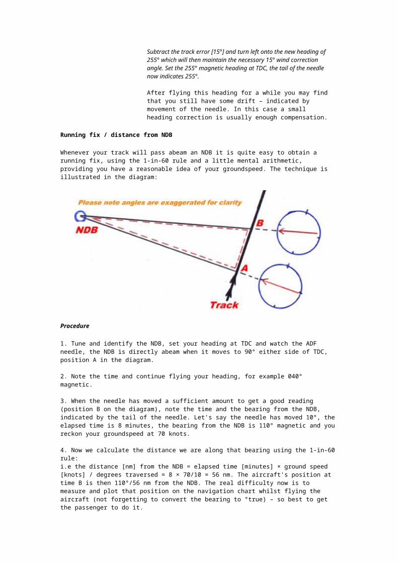
t h e i n s t r u m e n t l a n d i n g s y s t e m ( I L S )b y R.J.Bandet

In nearly 60 years of use ILS systems were never found at fault in an airplane Crash. This flawless record is a direct result of the training given to Navaid technicians. While training, technicians are told that the equipment cannot be allowed to operate outside the established tolerances. Any doubt and the equipment is shut down pending re-evaluation and recertification.

Brief description

The ILS usually consists of a Localizer, Glide Path, and Markers(OM, MM, & IM).

Localizer: This equipment provides lateral guidance to the runway centreline from about 5nm out.(five nautical miles).

Glide Path: This equipment provides the aircraft with a glide angle - usually 3 degrees. The Localizer and Glide Path combine to bring the aircraft to a point where the aircraft is 50 feet high at the runway threshold (decision point).

Markers:1. The Outer Marker at approximately 5nm helps the a/c adjust its course and height.2. The Middle Marker is located at approximately 3500 feet and used similarly.3. The Inner Maker at 1000 feet is used only for Category II operations.

Exceptions:There are always exceptions and here are some main exceptions.1. DME & GP (Distance Measuring Equipment & Glide Path) when it is impossible to have Markers.2. DME & Localizer when there is no GP for whatever reason.3. Offset Localizer. In this case the Localizer is not on the runway centreline, but offset and lined up to bring the aircraft over the threshold at decision height. Decision height is 50 feet at threshold.

click to enlarge in new window

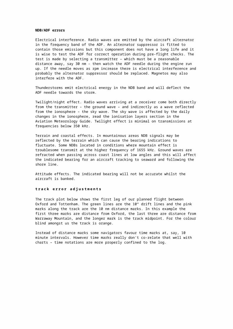
click to enlarge in new window

Localizer

The localizer is used to provide lateral guidance to the aircraft and thus allows for tracking the extended runway centreline. The localizer information is typically displayed on a course deviation indicator (CDI) which is used by the pilot until visual contact is made and the landing completed. The localizer radiates on a carrier frequency between 108 to 112 MHz with 50 kHz channel spacing. This carrier is modulated with audio tones of 90 Hz, 150 Hz, and 1020 Hz. The 1020 Hz tone is used for facility identification.

Normal limits of localizer coverage

IV. Glide Slope A. Frequency range: 329.15 - 335 MHz. B. Housed in a building next to the runway. C. 2.5 - 3 degrees above horizon. D. Used on front course only. E. Signal is 1.4 degrees wide. F. Automatically received with LOC frequency.

V. Marker Beacons A. ILS - outer and middle. B. LOC BC -- at FAF (BCM - back course marker) C. Outer marker (OM)

1. Located 4-7 miles from runway. 2. Indicates approximately where aircraft will intercept the glide slope when aircraft is

at the proper altitude. 3. Signal -- continuous dashes (2 per second). 4. Purple light.

D. Middle marker (MM) 1. Signal -- alternate dot/slash.

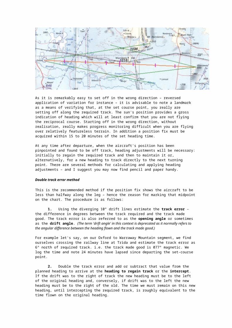
2. 3500' from landing threshold. 3. Amber light.

E. Back course marker (BCM) 1. Signal -- 2 dots. 2. White light. 3. Located at FAF of LOC BC approach.

F. Inner marker (IM) 1. Signal -- 2 dots. 2. White light. 3. Located between middle marker and landing threshold.

The localizer antenna array radiates two different signals, carrier plus sideband (CSB) and suppressed carrier sideband only (SBO). The CSB signal consists of the RF carrier amplitude modulated (AM) with equal amplitudes of 90 Hz and 150 Hz tones. The SBO signal is similar except that the carrier is suppressed. The localizer radiation patterns are normally arranged so that the course sector of the proportional guidance sector is symmetrical around the runway centreline (see figure).

If the aircraft on approach is aligned with the runway centreline, the CDI will display no difference in the depth of modulation (DDM) between the 90 Hz and 150 Hz audio tones; therefore, the CDI needle is centred.

If the aircraft is to the right of the centreline, the 150 Hz modulation will exceed that of the 90 Hz and produce a deflection on the CDI towards the left. Conversely, if the aircraft is to the left of the centreline, the 90 Hz modulation will exceed that of the 150 Hz and produce a similar but opposite deflection. This deflection corresponds to the direction the pilot must fly to be aligned with runway centreline and is proportional to the angular displacement from centreline.

The CDI has a full-scale deflection of 150 microamperes where the DDM equals 0.155 in both the 90 Hz and 150 Hz directions. The angular displacement, or proportional guidance sector, that corresponds to this full scale deflection is known as the localizer course width. This width is typically tailored for a full-scale CDI deflection to occur at 350 feet from runway centreline at threshold.

When the aircraft is outside this course guidance sector, the CDI is required to provide full scale deflection. This region is known as the clearance sector. The FAA requires that this region extend from the localizer course edge out to 35 degrees on both sides of centreline.

Reflected or scattered signals that come from hangars and buildings historically and today pose the greatest concern for establishing a localizer. These reflected signals cause quality derogation of the on-course signal as seen by the aircraft. To minimize these reflections, the common technique is to use larger array apertures that narrow the localizer course beam and thus reduce the quantity of signals incident on the reflecting surface.

In some cases, to maintain the ±35-degree clearance coverage, a separate RF carrier, offset from the course frequency by 8 kHz, is radiated. Since these two signals fall within the passband of the ILS receiver, the stronger of the signals is "captured" by the receiver and is used for the guidance. These two-frequency localizer arrays are called dual-frequency and are primarily used to support Category II/III operations.

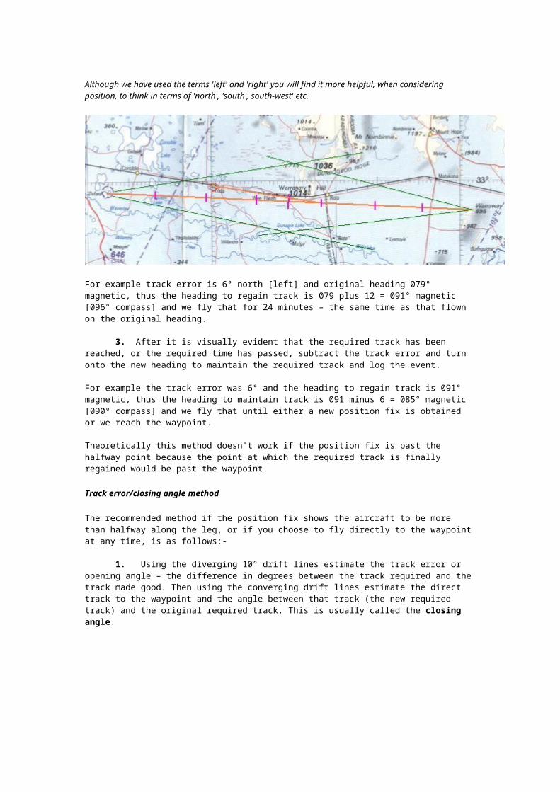
Glide Path

The glide slope provides the pilot with vertical guidance. This signal gives the pilot information on the horizontal needle of the CDI to allow the aircraft to descend at the proper angle to the runway touchdown point. The glide slope radiates on a carrier frequency between 329 and 335 MHz and is also modulated with 90 Hz and 150 Hz tones. The glide slope frequencies are paired with the localizer, meaning the pilot has to tune only one receiver control.  The radiation patterns of a typical glide slope system are similar to those of the Localizer - if you remember to rotate the pattern so that it is vertical instead of horizontal. The null in the sideband-only (SBO) signal produces essentially a straight glide path angle for the aircraft. The patterns are arranged so that 90 Hz modulation predominates above the glide path and the 150 Hz modulation predominates below.

The glide path angle is normally referenced at 3 degrees. If the aircraft is on this three-degree glide path, equal amounts of the 90 Hz and 150 Hz are received and the CDI will be centred. If the aircraft is above the glide path, the 90 Hz modulation exceeds that of the 150 Hz and produces a deflection on the CDI downwards. If the aircraft is below the established glide path, the 150 Hz modulation predominates and produces a similar but opposite deflection. This deflection corresponds to the direction the pilot must fly to intercept the glide path and is proportional to the angular displacement from the glide path angle. As with the localizer, the full scale deflection is 150 microamperes. Typically, the glide slope sensitivity is set so that the full-scale indications occur at approximately 2.3 and 3.7 degrees elevation.

The FAA presently maintains five types of glide slope systems. They are the null-reference, sideband-reference, capture-effect, endfire, and waveguide. The null-reference, sideband-reference, and capture-effect glide slope systems use the terrain in front of the antenna mast to double, effectively, the vertical aperture of the radiating system and produce the path in space. These three systems are typically referred to as image glide slope systems. Where the ground plane in front of the glide slope mast is irregular or absent, endfire or waveguide types are used. These systems are called non-image and do not rely on the terrain to form the path in space.

Marker Beacons

Inner, Middle, and Outer

Marker beacons are used to alert the pilot that an action (e.g., altitude check) is needed. This information is presented to the pilot by audio and visual cues. The ILS may contain three marker beacons: inner, middle and outer. The inner marker is used only for Category

II operations. The marker beacons are located at specified intervals along the ILS approach and are identified by discrete audio and visual characteristics (see Table 1). All marker beacons operate on a frequency of 75 MHz.

Marker Beacon Characteristics

Marker Beacon Pilot Alert Distance to Threshold Modulated frequency Audio Keying

Outer Glide Path Intercept 4 to 7nm 400Hz ------

Middle Category 1 Decision Height 3500 ft 1300Hz .-.-.-

Inner Category 2 Decision Height 1000 ft 3000Hz ......

 

 Table table 1

The marker beacon coverage provides adequate signal laterally throughout the localizer proportional guidance sector. Marker beacons produce cone or fan-shaped radiated patterns directed upward and, therefore, pose very few siting problems. The majority of problems in locating the marker beacon are the availability of real estate and access to utilities. If an acceptable site for the outer marker cannot be found, an alternative is to collocate a Distance Measurement Equipment (DME) transponder with the localizer. This DME then provides the range indication to the aircraft. The ILS models do not provide any information with regard to marker beacon performance.

t a c a n

Major system characteristics

System type Rotating beam beacon navigation system

Frequency band 962 - 1214 Mc/s

"Tacan" stands for "Tactical Air Navigation" and is a system which, working in the u.h.f. band, between 962 and 1,214 Mc/s, gives to a pilot continuous information as to his range and bearing from a beacon. The airborne equipment consists of an interrogating transmitter and a receiver which includes suitable demodulating circuits to enable the information contained in the beacon's response to be extracted. The ground equipment

consists of a beacon provided with a rotating aerial system. In the absence of interrogating signals the beacon transmits a series of random pulses together with groups of marker or reference pulses which are locked to the aerial rotation. Bearing information can be obtained without interrogation since the beacon is continuously transmitting.

In addition to transmitting a random series of pulses the beacon also periodically transmits a signal by which it identifies itself. To determine range the airborne transmitter radiates a series of pairs of pulses. These are received at the beacon and, after a fixed delay, are re-transmitted in place of the particular random pulses that the beacon would have transmitted in the absence of interrogation. The time delay between the emission of any interrogating pulse and the receipt of the reply is measured by one of the standard radar techniques described in Chapter 10. To avoid mistakes arising from multiple interrogation the airborne transmitter emits its pairs of pulses at random intervals. The receiver only recognises an exactly similar set of reply pulses all delayed by the same amount.

The aerial polar diagram of the beacon is of the shape shown in Fig. 3.13. This is produced by placing parasitic radiators, comprising a single radiator and a ring of nine, in the positions shown in Fig. 3.14.

By rotating these parasitic elements around the radiator the polar diagram is caused to rotate in space.

The parasitic elements spin round the aerial at 900 r.p.m. so that the received signal is amplitude modulated at 15 c/s, caused by the rotation of the single radiator, and at 135 c/s caused by the rotation of the group of nine radiators. A marker signal is transmitted every time the main lobe of the polar diagram passes due magnetic East. Somewhat misleadingly this is known as the "N " or north marker. Further marker signals are transmitted after

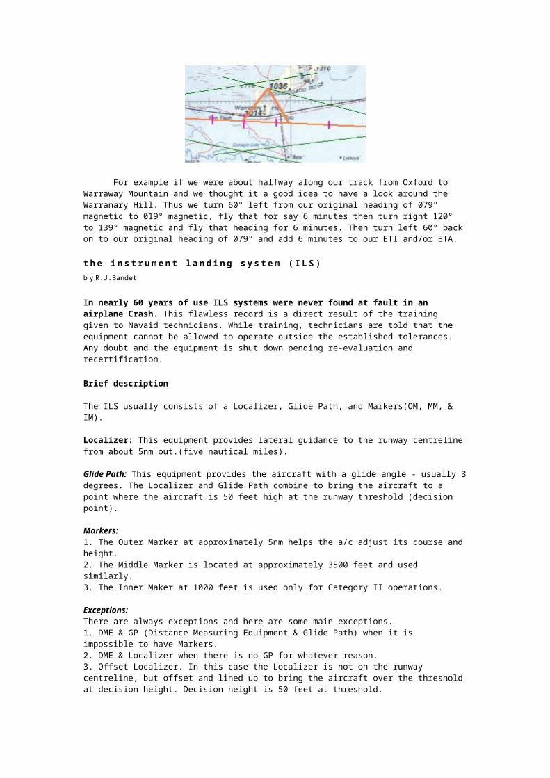
every 40o of rotation of the aerial pattern. This system of markers provides reference signals at 15 and 135 c/s for phase comparison with the signals received in the aircraft. As the aircraft flies round the beacon the time of receipt of the marker signals with respect to the phase of the amplitude modulation of the received signal varies as shown in Fig. 3.15.

The airborne receiver has five detectors. The first is an envelope detector whose output consists of a composite 15 and 135 c/s signal due to the rotation of the aerial pattern. The second and third detectors are used to isolate the 15 and 135 c/s reference signals respectively. The fourth detector is used to feed the range measurement circuits and the fifth to extract the beacon identification signal.

The signal from the envelope detector is passed through filters to separate the 15 c/s and 135 c/s modulations. A phase comparison circuit is used to measure the phase difference between the 15 c/s modulation and the 15 c/s reference signal from detector number two. This circuit enables the bearing of the beacon to be measured to within ±20o A second phase comparison circuit compares the phase of the 135 c/s modulation with that of the 135 c/s reference signal from detector number three. This gives the bearing of the beacon to an accuracy of about ±1o

There is no limit to the number of aircraft which can simultaneously obtain bearing information from a Tacan beacon but no more than 100 aircraft at a time can obtain distance information. The major claim of the Tacan system is that by employing an

antenna pattern comprising a main lobe and "ninth harmonic" lobes a nine-fold increase in accuracy is obtained. Whether such an accuracy can be obtained in varied conditions of siting has yet to be proved.

n a v i g a t i o n e n r o u t e ( a r e a n a v i g a t i o n )

RNAV

This type of navigation allows a pilot to fly a selected course to a predetermined point without the need to overfly ground-based navigation stations. Flight can be from waypoint to waypoint. A waypoint is a position determined either by Latitude/Longitude or Radial and distance from a VORTAC or VOR/DME station.

These navigation receivers use VOR/DME or VORTAC stations as a base point. A waypoint is defined as a distance along a radial of the VOR. The RNAV equipment electronically translates (moves) the VOR station to the waypoint position. You then fly the VOR as though it were located at the waypoint’s geographical location.

Through triangulation, the navigation unit measures the radial and distance of leg A. By knowing the entered data for leg B, the azimuth and distance to the waypoint along path C

is repeatedly calculated calculated. It is as though the VOR were located at the waypoint position.

Long Range Navigation (LORAN)

LORAN operates on the principle of time measurement. A Master station and up to to 4 secondary stations transmit a synchronized pulse. The time differential between the master station pulse and the secondary pulses is measured. From this data, the communication receiver can calculate the position of the aircraft within 0.25 Nm or better. The North East LORAN chain is shown. A database of airports and navigational facilities can be loaded into the memory of the LORAN unit.

The LORAN unit can indicate:

Present Position - in Latitude/Longitude and/or relative to a destination, waypoint or checkpoint. Bearing and distance to your destination. Groundspeed and estimated time enroute. Course Deviation Indicator. Storage in memory of all US airports, pilot selected fixes, minimum enroute and

obstruction clearance altitudes, and Class B and C airspace warnings. Continuous computation of bearings and distances to the nearest airports. Computation of

wind direction and velocity. Add ons, such as fuel flow analyzers to estimate fuel needed to reach destination and

alternates; ELT’s to transmit exact location of ELT.

Add-on programmable and updatable databases.

Since LORAN operates on a low-frequency signal, it is subject to the same disturbances that AM radio sustains. It is possible to loose signal when operating near thunderstorm and in heavy rain areas.

The LORAN receivers know the frequency of the Master and secondary stations; no tuning by the pilot is necessary.

Global Positioning System (GPS)

The GPS system is the latest in technology that can be used by aircraft. It has many of the attributes of LORAN. The complete system will contain up to 21 satellites in earth orbit. The "clocks" and "positional data" is updated periodically to insure accuracy of the data from

the satellites. It sense 4 or more satellites in orbit. The system is maintained by the US Department of Defence.

Like LORAN, it operates on a time-based methodology. Each satellite transmits coded pulses indicating it’s position, and the precise time the pulses are sent. The GPS unit listens to the satellite’s signal, and measures the time between the satellites transmission and receipt of the signal. By the process of triangulation among the several satellites being received, the unit computes the location of the GPS receiver. Not only can Latitude and Longitude be calculated, but altitude as well.

Like LORAN, the GPS unit contains data about all the commercial airports in the US, including runway lengths, directions, and location. There are numerous forms of display among the various manufacturer. The units can range from “hand held” to “panel mount” with altitude information input from an encoding altimeter. They can warn of Class B, C, and Prohibited and Restricted airspace. They can calculate direction and time to nearest suitable alternate airports in event of emergency.

The database in most units can be updated via a connection to a Personal Computer. The maximum error is within 100 meters (0.05 Nm). Work is in progress to give the GPS system adequate precision for instrument approaches.

No frequency tuning is required, as the frequency of the satellite transmissions are already known by the receiver.

Work is currently underway to provide sufficient accuracy for use of GPS for instrument approaches.

a t t i t u d e i n s t r u m e n t s fl y i n g

A . i n t r o d u c t i o n

The purpose of this section is to provide a brief review of the techniques of attitude instrument flight, including stall and stall recovery manoeuvres.

Attitude instrument flying is an extension of the concept of attitude flying. The establishment of a specific pitch and bank attitude, accompanied by a designated power setting, will cause predictable aircraft performance. Therefore, if pitch, bank and power are determined through reference to the flight instruments and the desired performance is confirmed by these instruments, the definition and technique of attitude instrument flight is clearly evident.

There are three basic ingredients to attitude instrument flying:

1. scan; 2. interpretation; and

3. aircraft control.

The human body is subject to sensations which are unreliable when interpreting the aircraft's actual attitude; therefore, the pilot must learn to disregard these sensations and control the aircraft through proper scan and interpretation of the flight instruments.

Proper scan is vital to the instrument pilot. Of course, instrument flying requires that certain instruments be used more often during particular manoeuvres. This is called selective radial scan. During a constant airspeed climb, for instance, the altimeter is less important than the airspeed indicator. Under instrument meteorological conditions, the pilot uses the attitude indicator to determine the aircraft's pitch and re-establish an attitude that will correct the airspeed to the desired value.

The attitude indicator replaces the normal outside visual references; therefore, it is the principal attitude control instrument for the radial scan. When scanning, the pilot should

regard the attitude indicator as the hub of a wagon wheel", and the other instruments as spokes. (see Attitude Indicator is Centre of Scan figure, below).

The second important ingredient in instrument flying is proper instrument interpretation. The attitude indicator provides an artificial horizon to replace the natural one; hence, proper interpretation is extremely important.

The last ingredient, aircraft control, results from scan and interpretation. It is simply a matter of applying the proper control pressures to attain the desired aircraft performance. These pressures are the same as in visual flight except that smaller and smoother control inputs are required.

B. instrument flying concept

The concept of control and performance attitude instrument flying can be applied. to any aspect of instrument flight. Under this concept, instruments are divided into three broad categories: control, performance and navigation.

1. control instruments: Control instruments indicate attitude of the aircraft and power (thrust/drag) being supplied to the aircraft. These instruments are calibrated to permit adjustments in definite amounts. They include the attitude indicator and engine control instruments (tachometer, manifold pressure, RPM, EPR).

2. performance instruments: Performance instruments indicate the actual performance of the aircraft, which can be determined from

the airspeed/mach, turn-and-bank, vertical speed indicators, altimeters, heading indicator, turn co-ordinator, magnetic compass.

3. navigation instruments: Navigation instruments indicate the position of the aircraft in relation to a particular navigational aid that has been selected. These can include NDB, VOR, ILS, INS, GPS, Loran-C, and OMEGA.

C. Attitude and power control

Proper control of aircraft attitude is the result of knowing when and how much to change attitude, and then smoothly changing it by a definite amount. Aircraft attitude control is accomplished by proper use of the attitude indicator. The attitude indicator provides an immediate, direct and corresponding indication of any change in aircraft pitch and/or bank attitude.

Pitch changes are accomplished by changing the pitch attitude of the reference line by set amounts in relation to the horizon bar. These changes are made in bat widths or degrees, depending upon the type of attitude indicator. On most attitude indicators a bat width represents approximately 2º of pitch change.

Bank changes are accomplished. by changing the bank attitude or bank pointers by set amounts in relation to the bank scale. Normally, the bank scale is graduated by 0º, 10º 20º, 30º, 60º and 90º, and this scale may be located at the top or bottom of the attitude indicator. Generally, an angle of bank that approximates the degrees to be turned is recommended; however, it should not exceed 30º in instrument flight. The TAS and the desired rate of turn are factors to be considered.

Proper power control results from the ability to smoothly establish or maintain desired airspeeds in co-ordination with attitude changes. Power changes are accomplished by throttle adjustment and with reference to the power indicators. Little attention is required to ensure that the power indication remains constant once it is established, because these indications are not affected by such factors as turbulence, improper trim or inadvertent control pressures.

D. trim technique

The aircraft has been correctly trimmed when it maintains a desired attitude with all control pressures neutralized. It is much easier to hold a given attitude constant by relieving all control pressures. In addition, more attention can then be devoted to the performance and navigation instruments and other cockpit duties.

First, apply control pressure to establish a desired attitude and then adjust the trim so that the aircraft will maintain that attitude when the flight controls are neutralized. Trim the aircraft for co-ordinated flight by centring the ball of the turn-and-slip indicator. This is done by using rudder trim in the direction the ball is displaced from centre.

Changes in attitude, power or configuration may require a trim adjustment. Independent use of trim to establish a change in aircraft attitude invariably leads to erratic aircraft control and is not recommended. Smooth and precise attitude changes are best attained by a combination of control pressures and trim.

E. scan technique

Scanning, or cross checking as it is sometimes known, is the continuous and logical observation of flight instruments. A methodical and meaningful instrument scan is necessary to make appropriate changes in aircraft attitude and performance.

The control and performance concept of attitude instrument flying requires that the pilot establish an aircraft attitude and power setting on the control instruments which should result in the desired aircraft performance. The pilot must be able to recognize the requirements for a change in attitude or power or both. By cross checking the instruments properly (scan), the pilot can determine the magnitude and direction of adjustment required to achieve the desired performance.

Scan can be reduced to the proper division of attention and interpretation of the flight instruments. Attention must be efficiently divided between the control and performance instruments and in a sequence that will ensure comprehensive coverage of the flight instruments. The pilot must quickly interpret what he or she sees when looking at the instruments and must become familiar with the factors to be considered in dividing his or her attention properly.

A factor influencing scan technique is the characteristic manner in which instruments respond to changes of attitude and power. The control instruments provide direct and immediate indications of attitude and power changes. Changes in the indications on the performance instruments will lag slightly behind changes of attitude or power. This lag is due to inertia of the aircraft and the operating principles and mechanisms of the performance instruments.

To develop the technique of always referring to the correct instrument at the appropriate time, you must continually ask yourself these questions:

1. What information do I need?

2. Which instruments give me the needed information?

3. Is the information reliable?

As mentioned earlier, the attitude indicator is the only instrument that the pilot should observe for any appreciable length of time. It is also the instrument that the pilot should observe the greatest number of times. An example of a scan demonstrates this; the pilot glances from the attitude indicator, then a glance at the airspeed indicator, back to the attitude indicator, and so forth (wagon wheel technique or radial scan). Of course different phases of flight will require slightly different scan techniques. This is called selective radial scan since the pilot will use particular instruments to carry out a particular task.

A correct or incorrect scan can be recognized by analyzing certain symptoms of aircraft control. Symptoms of insufficient reference to the control instruments are readily recognizable. The pilot should have some definite attitude and power indications in mind that should be maintained. If the performance instruments fluctuate erratically through the desired indications, then the pilot is probably not referring sufficiently to the control instruments. This lack of precise aircraft control is called chasing the indications.

Too much attention to the control instruments can be recognized by the following symptoms - if the pilot has a smooth, positive and continuous control over the indications of the control instruments but large deviations are observed to occur slowly on the performance instruments, a closer scan of the performance instruments is required.

The indications on some instruments are not as eye-catching as those on other instruments. For example, a 4º heading change is not as obvious as a 300 to 400-feet per-minute change on the vertical-speed indicator. Through deliberate effort and proper habit, the pilot must ensure that all the instruments are included in the scan. If this is accomplished, deviations on the performance instruments should be observed in their early stages.

A correct scan results in the continuous interpretation of the flight instruments, which enables the pilot to maintain proper aircraft control at all times. Remember, rapidly looking from one instrument to another without interpretation is of no value. Instrument systems and the location of the flight instruments vary. Pilot ability also varies. Therefore, each pilot should develop their own rate and technique of checking the instruments which will ensure a continuous and correct interpretation of the flight instruments.

F. adjusting attitude and power

The control and performance concept of attitude instrument flying requires the adjustment of aircraft attitude and power to achieve the desired performance in relation to the capabilities of your aircraft. A change of aircraft attitude and/or power is required when any indication other than that desired is observed on the performance instruments. However, it is equally important for the pilot to know what to change and how much of a pitch, bank or power change is required.

The phrase "Attitude plus power equals performance" summarizes the philosophy behind instrument flying. In other words, an aircraft's performance is the product of attitude and power. Performance is expressed in terms of airspeed, altitude, rate of climb or descent, or other criteria. If either attitude or power is changed, a change in performance will result.

The pilot knows what to change by understanding which control instrument to adjust to achieve the desired indications on the performance instruments. Bank attitude control is used to maintain a heading or a desired angle of bank during turns. Power control, in conjunction with a slight attitude change, may be used for maintaining or changing the airspeed while at a constant altitude. Power may also be used to establish a rate of climb or descent at a given airspeed or trim setting.

How much to adjust the attitude or power or both is, initially, an estimate based on familiarity with the aircraft and the amount the pilot desires to change the indications on the performance instruments. After making a change of attitude or power, the pilot should

observe the performance instruments to see if the desired change has occurred. If it has not, further adjustment is required.

To sum up, instrument flight is a continuous process of:

1. establishing an attitude and power setting on the control instruments; 2. trimming;

3. scanning, and

4. adjusting.

These procedural steps can be applied to any instrument manoeuvre and should result in precise attitude instrument flying.

Attitude Instruments Flying Manoeuvres

The following manoeuvres are described elsewhere for full and partial instrument panels and will not be duplicated here:

1. Straight-and-Level Flight; 2. Climbing;

3. Descending;

4. Turns;

5. Steep Turns;

6. Change of Airspeed; and,

7. Unusual Attitudes and Recoveries.

A. stalls and stall recovery

There are many different configurations from which to enter stall manoeuvres; however, for the purpose of this section, stalls will be discussed in reference to the realm of operations most frequently encountered in instrument flight. The entry procedures described are designed for training pilots to recover from induced stalls for training purposes. These manoeuvres should be accomplished in VMC at a safe altitude - normally with recovery planned for a minimum of 3000 ft. AGL. See the Aircraft Flight Manual for recommended procedures.

1. approach stalls

Straight-ahead: In the approach mode stall, the pilot establishes the aircraft in the configuration suitable for the type of aircraft, i.e., flaps and undercarriage positioned as specified in the aircraft flight manual as appropriate for an approach to landing.

The pilot must maintain altitude by constantly increasing elevator back pressure as the airspeed decreases toward the approach speed. When the approach speed is attained, the pilot should decrease the pitch attitude of the miniature aircraft in the attitude indicator to initiate a descent. When the aircraft is established in a constant-rate, straight-ahead descent at approach speed the pilot should increase the pitch attitude to approximately the second pitch reference line above the horizon (normally 10º) to purposely induce a stall in this configuration. The pilot must maintain the selected pitch attitude and remain on the heading from which the manoeuvre was begun.

The pilot should start recovery when buffeting begins, by simultaneously lowering the miniature aircraft to the horizon (or as required in the AFM) on the attitude indicator and

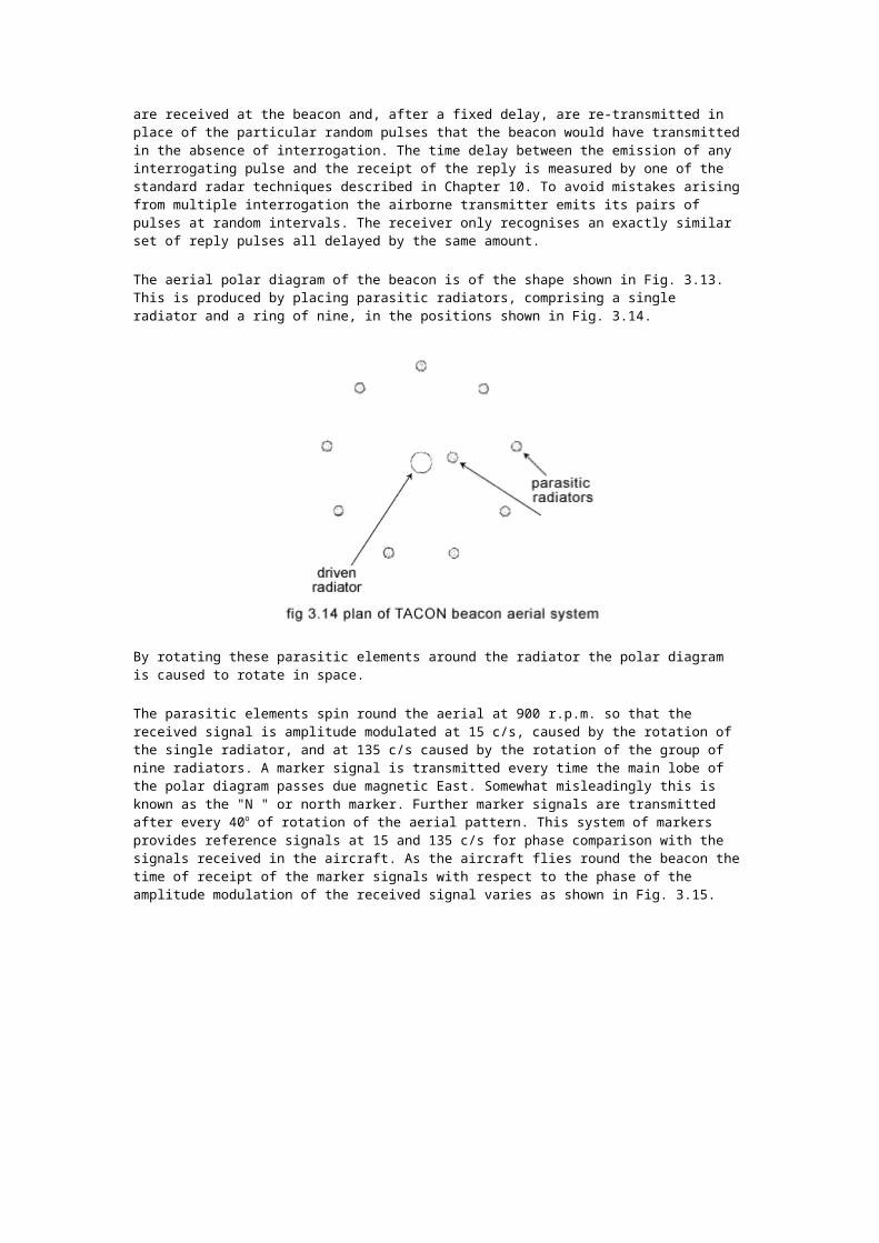
adding maximum allowable power. Maintaining the level flight attitude causes the airspeed to increase. Once the aircraft reaches a safe airspeed, the pilot should increase pitch to initiate a climb at this speed until reaching the altitude from which the manoeuvre began.

Turning: The pilot executes a turning approach stall in much the same manner as the straight-ahead approach stall (reducing power to the approach setting; maintaining altitude until the airspeed has decreased until the instrument indications have "settled down"). At this time the pilot increases the pitch attitude smoothly to the section pitch reference line above the horizon, and begins a 15º - 20º bank turn in either direction. The pilot maintains the pitch and bank through the use of the attitude indicator until buffeting occurs.

The recovery procedure is the same as for the straight-ahead approach stall except that the wings are to be levelled and the recovery heading is maintained.

2. take-off and departure stalls

Straight-ahead: The pilot reduces power to flight idle, or approximately 15 in. Hg manifold pressure, and maintains altitude, using the attitude indicator, vertical speed indicator and altimeter as references. As the airspeed decreases to lift-off speed, the pilot sets a wings-level, straight-ahead climb and increases power at a pitch angle that causes a

power-on, straight-ahead stall.

The pilot accomplishes this by adjusting the pitch of the miniature aircraft to the second pitch reference line above the horizon (or as required in the aircraft type). The pilot must also maintain the initial heading until a stall buffet occurs. As the airspeed decreases, the pilot must increase back elevator pressure to hold the pitch attitude selected. Direction and control must be maintained strictly by use of the rudder.

When the buffet occurs the pilot should pitch down to the horizon bar, add maximum allowable power and allow the aircraft to accelerate. The recover altitude should be maintained and the manoeuvre completed on the same heading as used throughout the stall. After attaining climb airspeed, the pilot should reduce power to the climb setting.

turning: The turning take-off and departure stall begins in the same manner as the straight-ahead departure stall. The pilot reduces power and maintains altitude. As the airspeed decreases to lift-off speed,

the pilot increases the pitch to the second pitch reference line, applies increased power and a makes a 15º to 20º bank in either direction. The pilot maintains this climbing turn attitude on the attitude indicator until a stall buffet occurs. To recover, the pilot lowers the pitch attitude to the horizon bar, levels the wings and maintains the recovery altitude and heading. As the airspeed approaches climb, the pilot should reduce power to the climb setting.

u n d e r s t a n d i n s t r u m e n t a p p r o a c h p l a t e s

 

Approach Plates (Instrument Approach Procedures) are one of the greatest tools used for Instrument Navigation as well as VFR Flying. Without these vital diagrams, landings in poor

weather would be near impossible. Each drawing is full of essential information that, when pieced together properly, provide all the necessary navigation to transition from air to ground.

This lesson is broken up into FOUR sections concentrating on the main areas of the Approach Plate diagram. The diagram used is a basic VOR Approach that describes most features of common approach plates.

 

It is a big decision. You have wanted to fly for some time and now you're going to do it. Excitement. Anticipation. You go to the airport and they take you out to the plane you are going to fulfil your dream of learning to fly in and… The plane is older than you are. It looks its age. It smells its age. It shakes, rattles and rolls. It squeaks. The plastic or Royalite is cracked and sun faded. Well, you get the idea.

Click on a highlighted area to learn about it.

Plan View

The Plan View shows a depiction as if looking down on top of the airfield, NAVAIDS and terrain. It shows the basic flight path to follow as well as other helpful items.

This overhead view is used primarily to get the plane to the approach area as well as directional guidance needed for alignment with the proper approach route. Once inside the 10nm circle, everything is drawn to scale for better use.

It also provides locations of fixes, intersections, points, radials, holding areas, missed approach turns, and more !

 Click on a highlighted area to learn about it.

The Profile View / Approach Minima Section

The Profile view is a side look at the approach start - to - finish. This view concentrates on showing elevation changes as you approach the runway. It uses most of the same symbols as the Plan View.

The principle purpose of the Profile View is to show how your altitude will change as you fly along the Procedure Track(s) towards the airfield.

The Approach Minima Section contains altitude restrictions that correlate with the approach speed of your aircraft. These altitudes are RESTRICTIVE altitudes that you must fly while at certain phases of the approach. They are intended to provide you with obstacle- traffic clearance and smooth altitude transitions while on the approach.

Click on a highlighted area to learn about it.

The Field Diagram

The Field Diagram is an overhead look at the airfield and runways. It shows us small details needed for our approach such as runway lengths, lighting, arresting gear, elevations, etc..

This diagram also includes Final Approach Fix - Missed Approach point TIMES when using an approach that does not require DME.

G l o s s a r y o f T e r m s term brief definition

Approach- The transition from standard flight in preparation to land.

DME- Distance Measuring Equipment. This system allows us to use radio signals to determine distance from the transmitting station.

FAF- see Final Approach Fix

Final Approach Fix- The point where we begin our transition down to the airfield, TOWER gives us further clearance to land here, also where we can descend to the MDA.

HAA- see Height Above Airport

HAT- see height Above Touch-down-zone

Height Above Touch-down-zone-

The distance in feet, above the touchdown area of the runway that is used to compute the Minimum Descent Altitude (MDA) or Decision Height (DH).

IAF- see Initial Approach Fix

INT- Intersection

Initial Approach Fix- Point where the decision to land or go around must be made

MAP- see Missed Approach Point

MDA- see Minimum Descent Altitude

Minimum Descent Altitude-

The altitude restriction placed after the FAF that you can not descend below UNTIL you have visual of the runway environment.

Missed Approach- Basically, re-positioning your aircraft to gain altitude and clear of traffic / obstacles, in preparation for another approach.

Missed Approach Point- Point where the decision to land or go around must be made

VOR- VHF Omni-directional Range. Use to transmit Magnetic Bearing information along 360 radials. No Distance information is sent unless DME accompanies the VOR system.