radio propagation prediction for hf...

Communications 2018; 6(1): 5-12

http://www.sciencepublishinggroup.com/j/com

doi: 10.11648/j.com.20180601.12

ISSN: 2328-5966 (Print); ISSN: 2328-5923 (Online)

Radio Propagation Prediction for HF Communications

Courage Mudzingwa, Albert Chawanda

Department of Applied Physics & Telecommunications, Midlands State University, Gweru, Zimbabwe

Email address:

To cite this article: Courage Mudzingwa, Albert Chawanda. Radio Propagation Prediction for HF Communications. Communications. Vol. 6, No. 1, 2018, pp. 5-12.

doi: 10.11648/j.com.20180601.12

Received: December 30, 2017; Accepted: February 6, 2018; Published: February 27, 2018

Abstract: The refraction and apparent reflection of HF radio waves by the ionosphere enables long range HF radio

communications. The ionosphere is a distinctly irregular medium that is mostly driven by solar activity. Ionospheric models are

useful in the prediction of ionospheric behaviour and in the provision of data required for the analysis and forecasting of

ionospheric propagation. This paper provides a compact review of HF radio propagation prediction techniques and approaches

for HF communications. The paper also highlights the numerous approaches have been used to date in an attempt to estimate F2

usable frequencies. The review presented in this paper is inspired by the most recent advances in the field of ionospheric

prediction and modelling.

Keywords: HF Communications, Propagation Prediction, Ionosphere, Usable Frequency, MUF

1. Introduction

The forecasting of radio wave propagation is considered as

an applied science. However, for the past four to eight

decades, models for long term forecasting of the median

monthly conditions for HF radio propagation have

represented an important tool not only for applied science

and radio science but also for geophysical researchers in their

theoretical studies of the upper atmosphere [1-3]. The main

aim of radio propagation forecasting is not only to increase

knowledge but rather to improve communication systems.

HF communication is used for short and long range tactical

and strategic military purposes since its antennas and

equipment can be deployed rapidly to provide immediate

command post communications without the need for careful

site planning, as is the case with line of sight (LOS)

communications. In civilian society, HF is used for

international broadcasts by organizations such as the British

Broadcasting Corporation and the Voice of America [3]. In

Southern Africa, HF exploitation is relatively common and is

a primary method for communication since satellite

communication infrastructure is not as well improved as in

the developed countries. As a result, the use of HF

communication is preferred due to its relative simplicity, its

capability to provide long range communication at low power

without repeater base stations, its ease of development and its

low cost [4].

The main purpose of radio propagation forecasting is to

give advice in advance about the future reliability of

frequency bands propagated by means of the ionosphere.

This task is referred to as long-term prediction/forecasting

and can be split into a geophysical one, forecasting of a

model ionosphere, and one of optical-electromagnetic theory,

resolution of the propagation problem [2]. The information

about the ionosphere may be called input; the prediction

produced in the process is the output. One uses simplified

models for the ionosphere and for propagational phenomena,

selecting those features of both which have greater influence.

Generally there is no unique solution of the forecasting

problem; the right effort has to be found in a compromise

between the needs of the user or client and the available

resources [2, 5].

2. Ionospheric HF Propagation

The ionosphere is an ionised region of the Earth's upper

atmosphere which ranges from about 50 km to about 1000

km. The extent of ionospheric refraction depends on the

density of ionization of the layer, the frequency of the radio

wave and the angle at which the wave enters the layer [6]. In

order to successfully propagate radio waves through the

ionosphere, the frequency cannot be too small, as the wave

would then be absorbed, nor too high, for reflection would no

6 Courage Mudzingwa and Albert Chawanda: Radio Propagation Prediction for HF Communications

longer be possible in this case. The two frequencies thus

defined are referred to as the lowest usable frequency (LUF)

and the maximum usable frequency (MUF) respectively.

The MUF is determined by the degree of ionisation in the

ionospheric layer, while the LUF is generally determined by

the multihop path attenuation and the noise level at the receive

site. The frequency of optimum transmission (FOT) or

optimum working frequency (OWF) is the frequency with

maximum availability and minimum path loss, and it is

generally taken as a percentage of the MUF [5]. The incident

angle at which a radio wave enters the ionosphere determines

the extent to which that particular wave and the maximum

distance that may be covered in a single hop is 4000 km.

Figure 1. Simplified scheme of an HF radio link [1].

Considering application and operational reasons, HF

propagation is basically split into skywave, groundwave and

near vertical incidence (NVI). Groundwave propagation is

used for relatively short links over a few tens of kilometres

whereas skywave propagation can be used worldwide, in

suitable ionospheric conditions. Groundwave propagation is

affected by the earth’s conductivity while skywave

propagation is dependent on ionospheric conditions and the

effects of the sun. NVI propagation is used for short range HF

radio communication. The antenna plays a critical role in NVI

propagation by radiating its main beam at a very high take off

angle (TOA). The ionosphere is important to skywave radio

propagation and provides the basis for almost all HF

communications beyond LOS [7-9]. The ionosphere is also

essential in optimising satellite communication systems since

the satellite signals traverse the ionosphere, leading to

attenuation, depolarization, refraction and dispersion as a

result of scattering and frequency dependent group delay.

When an HF radio wave reaches the ionosphere, it can be

refracted such that it radiates back toward the Earth at some

horizontal distance beyond the horizon (see Figure 1). This

effect is due to refraction but it is often apparently considered

to be a reflection, following Bouguer’s refraction law [10].

Figure 1 shows a simple scheme of an HF radio link

demonstrating that the behaviour of different electromagnetic

rays depends on the angle of elevation β. In Figure 1 rays a

and b, with a small angle of incidence φ to the ionosphere,

escape into space, rays c, d, e, and f, with an angle of incidence

greater or equal than φ, are reflected by the ionosphere.

Intercontinental broadcasting and communication on HF

bands are achieved through ionospheric propagation using the

skip phenomenon (as illustrated in Figure 1). Rays reflected

by the ionosphere will arrive at greater distances until the

elevation angle β is tangential to the ground. The skip distance,

also known as the silent zone, is the minimum distance that a

ray coming back from the ionosphere is reflected. Within the

skip distance, only ground wave propagation is possible [7-9,

11].

With increasing antenna take off angle (TOA), τ (from

Figure 2), refracted penetration occurs and the signal is not

reflected back to earth. A lower TOA will increase the distance

of the first reflection off the F layer of the ionosphere [11].

This increased distance will enhance long-range signal

propagation. However, all around the transmitter, a skip zone

exists where no reflected rays are received [2].

Figure 2. True (solid line) and equivalent (dashed line) trajectories of HF

radio waves between two points on Earth through skip mode.

In 1931 Plendl explained the effects of the 11 year solar

cycle variation on HF communications [12]. By 1939 it was

already known that diurnal conditions also greatly influenced

Communications 2018; 6(1): 5-12 7

the ionospheric communications [13]. In 1937 Smith

developed a prediction method of determining the virtual

reflection height, for a given frequency f, of a triangular path

covering the given transmission link (Tx to Rx, as indicated in

Figure 2) [14]. Smith assumed isotropic dispersion, plane

geometry and applied Snell’s refraction law [15]. For a curved

ionosphere and curved earth, ignoring the effects of the

Earth’s magnetic field the refractive index n of the ionosphere

is given by: [16].

�� = 1 − �� (1)

where: f is the wave frequency and fp is the plasma frequency.

Using the layered approximation to the ionosphere to predict

the ray bending, thus a ray entering the ionosphere at an angle

of incidence � will be reflected at a height where the

ionisation is such that n has the value [17, 18]:

� = � �� (2)

At vertical incidence the reflection condition occurs when n

equals zero and from (1) this occurs where � = ��. If � = ��

represents the vertically incident frequency reflected at the

level where the plasma frequency is �� then for the obliquely

incident wave:

� �� = 1 − �� = 1 − �� (3)

Therefore:

�� = �� (4)

Thus an oblique frequency �� incident on the ionosphere

at an angle � will be reflected from the same true height as

the equivalent vertical incidence frequency hence a given

ionospheric layer will always reflect higher frequencies at

oblique incidence than at vertical incidence [7-9]. When �� has its maximum value, the frequency � is called the

maximum usable frequency (MUF), hence:

�� = �� (5)

Since �� changes as the ionosphere changes, it is

therefore sufficiently accurate to introduce a correction factor � (Smith’s coefficient) so that the secant law in (4) becomes

(5) [14, 15, 19, 20]. The constant � is a function of path

length (D) and reflection height (ℎ�). From Figure 2, using the law of sines of triangles, � in (5)

can be expanded to: [21]

� = arctan " #$%�& �'() *+,- '() ./0#�& �'() 1 (6)

where:

2 = 3 256) (7)

� – ray incidence angle, ℎ� – virtual height, D – distance

between Tx and Rx, M – path midpoint, 56 – Earth’s radius

and 7 – ray take-off angle.

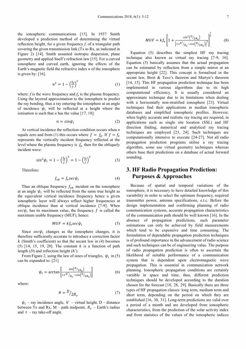
�� = �� 81 + :�;<�& �'() =*+,- '() .>�:�& �'() ?<@

A< (8)

Equation (5) describes the simplest HF ray tracing

technique also known as virtual ray tracing [7-9, 16].

Equation (5) basically assumes that the actual propagation

can be estimated by reflection from a simple mirror at an

appropriate height [22]. This concept is formalised in the

secant law, Breit & Tuve’s theorem and Martyn’s theorem

[14, 15]. This HF propagation prediction technique has been

implemented in various algorithms due to its high

computational efficiency. It is usually considered an

approximate technique due to its limitations when dealing

with a horizontally non-stratified ionosphere [23]. Virtual

techniques find their applications in median ionospheric

databases and simplified ionospheric profiles. However,

when highly accurate and realistic ray tracing are required, in

applications such as single site location (SSL) and HF

direction finding, numerical and analytical ray tracing

techniques are employed [23, 24]. Such techniques are

computationally intensive to execute [24-27]. Not all radio

propagation prediction programs utilise a ray tracing

algorithm, some use virtual geometry techniques whereas

others base their predictions on a database of actual forward

sounding.

3. HF Radio Propagation Prediction:

Purposes & Approaches

Because of spatial and temporal variations of the

ionosphere, it is necessary to have detailed knowledge of this

variability in order to select the optimum frequency, required

transmitter power, antenna specifications, e.t.c. Before the

design implementation and confirming planning of radio

communication systems, accurate propagation characteristics

of the communication path should be well known [16]. In the

absence of propagation predictions, such parameter

estimations can only be achieved by field measurements

which tend to be expensive and time consuming. The

formulation of dependable propagation prediction techniques

is of profound importance in the advancement of radio science

and such techniques can be of engineering value. The purpose

of radio propagation prediction is often to ascertain the

likelihood of suitable performance of a communication

system that is dependent upon electromagnetic wave

propagation. This is essential in communication network

planning. Ionospheric propagation conditions are certainly

variable in space and time, thus, different prediction

techniques should be developed according to the duration

chosen for the forecast [18, 28, 29]. Basically there are three

types of HF propagation classes: long term, medium term and

short term, depending on the period on which they are

established [16, 30, 31]. Long-term predictions are valid over

a period of a month and are developed from ionospheric

characteristics, from the prediction of the solar activity index

and from statistics of the values of the ionospheric indices


measured during previous similar situations [32]. Long-term

predictions are useful for frequency management, circuit and

service planning as well as radio system design and testing.

This type of prediction has an important role in the provision

of information on the choice of frequency range, Tx location,

Tx power and the selection of suitable Tx and Rx antennas.

Medium-term predictions are intended at forecasting the

general propagation conditions and particularly the MUF

values during the next week period [30]. Such predictions are

meant for the correction and adaptation of long-term

ionospheric forecasts with respect to season as well as solar

and geomagnetic activities. The fundamental characteristics of

these predictions are therefore their more accurate

approximation of seasonal variations and their better account

of solar and magnetic activities. On the other hand, short-term

predictions are generally stipulated over the next 24 hours and

are intended at forecasting the usable frequency band over six

hour periods in comparison with the usable frequency band

defined over the long term. These short-term predictions are

meant for providing corrections of long-term forecasts on a

daily basis over permanent areas [33]. As a result, they

generally refer to departures from the median behaviour.

Short-term frequency predictions are required by the circuit

operator in order that he may be able to anticipate MUF failure

and thus increase the circuit reliability. Short-term ionospheric

fluctuations may be specified in terms of hourly, daily and

weekly variabilities. There are also second-to-second and

minute-to-minute variations but this group of variations

broadly falls within the sphere of unpredictable behaviour.

These very short-term predictions are generally referred to as

nowcasts [34]. The most common ionospheric short-term

fore-casting methods at present mainly include

auto-correlation function method, multiple linear regression

method, artificial neural network method, equivalent sunspot

number method, Kalman filtering method, similar day method,

storm time ionospheric forecasting method and so on [35-37].

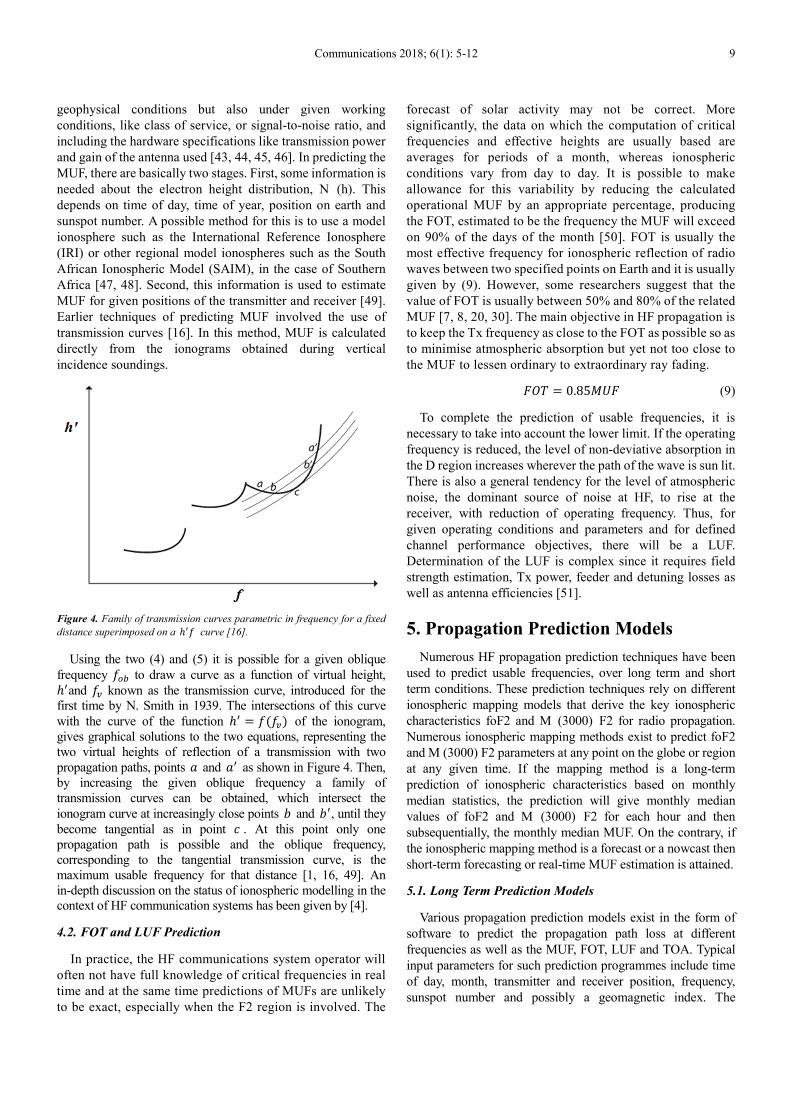
Figure 3. Variations in LUF, MUF and FOT over a 24-hour period.

Figure 3 shows a typical variation of LUF, MUF and FOT

over a day. This diagram is indicative only; in practice, it will

vary from location to location and between successive days,

weeks and months [28]. Apart from the reliance on the

geographic location of Tx and Rx, HF propagation conditions

of an ionospheric transmission link between two points on the

earth vary with daytime, season, and the solar cycle. As a

result, it is important to predict the parameters for optimum

operational frequencies and other radio propagation

applications. Such parameters include the MUF, LUF, FOT

and TOA. In the provision of ionospheric services, prediction

of ionospheric conditions through time and space has always

been a major component. It has been well documented that for

F region modelling the critical frequency of the F2 layer foF2

and its propagation factor M (3000) F2, depend systematically

on measurable quantities closely related to solar radiation [22,

38-40]. Ionospheric and solar indices generated from both

ionospheric and solar data provide a quick and proxy measure

of the complex ionospheric response to variations in solar

activity and hence they are useful in mapping the temporal

variation of the ionospheric parameters relevant to

propagation prediction. On the other hand, the F1 and E layers

have a less complex morphology and Chapman’s

approximations provide an adequate temporal and spatial

description for the same purposes [41].

4. F2 Usable Frequency Prediction

The F2 layer is considered as the principal ionospheric layer,

which also determines the long-range propagation of HF radio

waves. Over the years, ionospheric prediction and modelling

under specific geophysical conditions has proved to be

complex. Usable frequency prediction in HF communications

is the foundation of high frequency management. In planning

the best use of a given radio communication link, it is

important to know in advance what frequencies can be used so

as to counter the variability of the ionosphere. Choosing the

correct frequency is fundamental to maintaining acceptable

communications. The successful choice of the most

appropriate frequency depends on the ability to predict and

respond to the prevailing ionospheric conditions.

4.1. MUF Prediction

It is usually desirable for HF transmission to occur on a

frequency as near to the maximum usable frequency over the

path at any instant as is feasible under conditions prevailing in

practice. We therefore need to know the MUF. In the early

days of ionospheric communications, the term ''maximum

usable frequency" was used without regard to the meaning of

''usable" [16, 42]. To standardise the MUF definition, the

International Radio Consultative Committee (CCIR) adopted

the following recommendation: (i) Basic MUF is the highest

frequency of propagation between two points of an HF radio

link established only by ionospheric reflection and permitted

by the geophysical conditions along the radio path. (ii)

Operating MUF is the highest frequency that permits a radio

link between two points not only under ionospheric and


geophysical conditions but also under given working

conditions, like class of service, or signal-to-noise ratio, and

including the hardware specifications like transmission power

and gain of the antenna used [43, 44, 45, 46]. In predicting the

MUF, there are basically two stages. First, some information is

needed about the electron height distribution, N (h). This

depends on time of day, time of year, position on earth and

sunspot number. A possible method for this is to use a model

ionosphere such as the International Reference Ionosphere

(IRI) or other regional model ionospheres such as the South

African Ionospheric Model (SAIM), in the case of Southern

Africa [47, 48]. Second, this information is used to estimate

MUF for given positions of the transmitter and receiver [49].

Earlier techniques of predicting MUF involved the use of

transmission curves [16]. In this method, MUF is calculated

directly from the ionograms obtained during vertical

incidence soundings.

Figure 4. Family of transmission curves parametric in frequency for a fixed

distance superimposed on a ℎ�� curve [16].

Using the two (4) and (5) it is possible for a given oblique

frequency �� to draw a curve as a function of virtual height, ℎ�and �� known as the transmission curve, introduced for the

first time by N. Smith in 1939. The intersections of this curve

with the curve of the function ℎ� = �B��C of the ionogram,

gives graphical solutions to the two equations, representing the

two virtual heights of reflection of a transmission with two

propagation paths, points D and D� as shown in Figure 4. Then,

by increasing the given oblique frequency a family of

transmission curves can be obtained, which intersect the

ionogram curve at increasingly close points E and E�, until they

become tangential as in point � . At this point only one

propagation path is possible and the oblique frequency,

corresponding to the tangential transmission curve, is the

maximum usable frequency for that distance [1, 16, 49]. An

in-depth discussion on the status of ionospheric modelling in the

context of HF communication systems has been given by [4].

4.2. FOT and LUF Prediction

In practice, the HF communications system operator will

often not have full knowledge of critical frequencies in real

time and at the same time predictions of MUFs are unlikely

to be exact, especially when the F2 region is involved. The

forecast of solar activity may not be correct. More

significantly, the data on which the computation of critical

frequencies and effective heights are usually based are

averages for periods of a month, whereas ionospheric

conditions vary from day to day. It is possible to make

allowance for this variability by reducing the calculated

operational MUF by an appropriate percentage, producing

the FOT, estimated to be the frequency the MUF will exceed

on 90% of the days of the month [50]. FOT is usually the

most effective frequency for ionospheric reflection of radio

waves between two specified points on Earth and it is usually

given by (9). However, some researchers suggest that the

value of FOT is usually between 50% and 80% of the related

MUF [7, 8, 20, 30]. The main objective in HF propagation is

to keep the Tx frequency as close to the FOT as possible so as

to minimise atmospheric absorption but yet not too close to

the MUF to lessen ordinary to extraordinary ray fading.

�FG = 0.85�� (9)

To complete the prediction of usable frequencies, it is

necessary to take into account the lower limit. If the operating

frequency is reduced, the level of non-deviative absorption in

the D region increases wherever the path of the wave is sun lit.

There is also a general tendency for the level of atmospheric

noise, the dominant source of noise at HF, to rise at the

receiver, with reduction of operating frequency. Thus, for

given operating conditions and parameters and for defined

channel performance objectives, there will be a LUF.

Determination of the LUF is complex since it requires field

strength estimation, Tx power, feeder and detuning losses as

well as antenna efficiencies [51].

5. Propagation Prediction Models

Numerous HF propagation prediction techniques have been

used to predict usable frequencies, over long term and short

term conditions. These prediction techniques rely on different

ionospheric mapping models that derive the key ionospheric

characteristics foF2 and M (3000) F2 for radio propagation.

Numerous ionospheric mapping methods exist to predict foF2

and M (3000) F2 parameters at any point on the globe or region

at any given time. If the mapping method is a long-term

prediction of ionospheric characteristics based on monthly

median statistics, the prediction will give monthly median

values of foF2 and M (3000) F2 for each hour and then

subsequentially, the monthly median MUF. On the contrary, if

the ionospheric mapping method is a forecast or a nowcast then

short-term forecasting or real-time MUF estimation is attained.

5.1. Long Term Prediction Models

Various propagation prediction models exist in the form of

software to predict the propagation path loss at different

frequencies as well as the MUF, FOT, LUF and TOA. Typical

input parameters for such prediction programmes include time

of day, month, transmitter and receiver position, frequency,

sunspot number and possibly a geomagnetic index. The


geomagnetic index is used in programmes which use special

models for high latitudes. Due to the variations and uncertainty

in ionospheric conditions, prediction models can only give

statistical information. ICEPAC is an enhanced IONCAP

(Ionospheric Communications Analysis and Prediction) model

developed by the Institute of Telecommunications Sciences

(ITS) in Boulder, Colorado, during the 1970s [52]. ICEPAC is a

full system performance model for HF radio communications

circuits in the frequency range of 2 to 30 MHz. It was designed

to predict HF sky wave system performance and analyse

ionospheric parameters. ICEPAC was developed with a much

more elaborate high-latitude ionospheric model called

Ionospheric Conductivity and Electron Density (ICED), taking

the geomagnetic Q index as an additional input parameter. The

computer programme is an integrated system of subroutines

designed to predict HF sky wave system performance and

analyse ionospheric parameters. ICEPAC predictions require

user-defined input data, such as the year, month, day, frequency

of operation, type of antenna used, the transmitter power, the

type of propagation prediction required and the man-made

noise environment, among others [53]. The Australian

Government IPS Radio and Space Services HF propagation

prediction method is known as the Advanced Stand Alone

Prediction System (ASAPS) and is able to predict sky wave

radio communication conditions for both the HF and VHF radio

spetra. ASAPS was developed by the IPS Radio and Space

Services of the Australian Bureau of Meteorology, merges the

features of the original IPS method with the ITU-R/

International Radio Consultative Committee (CCIR) models.

Numerous graphic representations are based on this method

according to the different needs of clients. The graphs have

regional or even global validity. The Simplified Ionospheric

Regional Model & Lockwood (SIRM&LKW) is a monthly

median MUF prediction method for a point to point radio link.

SIRM&LKW is based on an empirical method supported by the

Istituto Nazionale di Geofisica e Vulcanologia (INGV) for

ionospheric HF propagation prediction conditions over the

Mediterranean area. In SIRM&LKW, the predicted foF2 and M

(3000) F2 are derived from the monthly median SIRM and foE

input values come from the Chapman model [54]. Previous

research has confirmed that usable frequencies of an HF

communications link can be predicted, with considerable

accuracy, using existing HF propagation prediction models

such as REC533 and VOACAP. Various fundamental

approaches have also been established for handling the

short-term ionospheric variability in HF propagation prediction.

Good examples, with varying levels of sophistication, can be

found in HF propagation tools such as: HF-EEMS [55] and

OpSEND [56] while others are still in development. Extensive

research on propagation prediction techniques has been covered

by [1, 57-59].

5.2. Nowcasting Models

Nowcasting refers to merging ionospheric models with real

time or near real time foF2 and M (3000) F2 observations,

providing users with real time or near real time maps as well

as an accurate representation of prevailing ionospheric

conditions. The intergration of prediction models and

real-time ionospheric measurements in the development of

lucid regional or global maps, in line with recent observations,

is the basis for nowcasting. The number of nowcasting models

has increased in recent years, this includes the SIRM Updating

Method & Lockwood (SIRMUP&LKW), Instantaneous

Space Weighted Ionospheric Regional Model (ISWIRM) and

SAIM, for the Southern African region. SIRMUP&LKW

model predicts the daily hourly MUF values by using the

nowcasting SIRMUP model to derive foF2 and M (3000) F2

parameters [60]. ISWIRM is a regional foF2 nowcasting

model, applicable within the geographic range between 35o -

70°N and 51°W - 40oE. Within this geographic region, the

hourly values of foF2 are obtained correcting the monthly

medians values of foF2, predicted by the Space Weighted

Ionospheric Local Model (SWILM) [61], basing on hourly

foF2 observations from four reference ionosondes. For

in-depth detail on the development of SAIM, refer to [48].

6. Limitations to Accurate F2 Usable

Frequency Prediction

The successful prediction of F2 usable frequencies depends

on the accuracy of F2 peak parameter prediction, hence

limitations to accurate F2 predictions has a cumulative effect

on F2 usable frequency predictions. Notable limitations to

accurate F2 usable frequency prediction includes:

1. The relationships governing the global distribution of

ionospheric parameters as a whole are still not

completely understood [62].

2. There is no widely adopted morphology of the F2 region

at nighttime, rendering the interpretation of nighttime

diurnal variations complex. Since various types of

nighttime enhancements in the F2 layer electron

concentration manifest, nighttime F2 layer related

predictions may be much less accurate than daytime

predictions. [63, 64].

3. The unavailability of complete knowledge of the F2

layer in its perturbed state poses major limitations, not

only on the prediction of usable frequencies, but also on

interpreting the complexities surrounding the spatial and

temporal evolution of the perturbation effect. Besides,

apart from the beginning of cyclical geomagnetic

disturbances, the prediction of temporal variation of

disturbances a few hours or more in advance is not yet

possible [65].

4. The reliability of ionospheric parameter prediction is

determined by precise and dependable knowledge about

the evolution of the ionosphere as well as the accuracy

and absoluteness of inputs which are used in predictive

computations.

7. Conclusion

This paper has reviewed and analysed various techniques

and approaches that have been used to date in predicting or


forecasting ionospheric parameters and F2 usable frequencies.

The intricacy in the prediction of MUF, FOT, TOA and LUF

was also discussed while highlighting the subsequent

limitations that affect the accuracy of F2 propagation

predictions.

References

[1] B. Zolesi and L. R. Cander, Ionospheric Prediction and forecasting, Springer, New York, 2014.

[2] K Rawer, The historical development of forecasting methods for ionospheric propagation of HF waves, Radio Sci, vol 10, no. 7, pp. 669-679, 1975.

[3] L. Barclay (ed), Propagation of radio waves, The institution of Engineering and Technology, UK, 2003.

[4] J. M. Goodman, Operational communication systems and relationships to the ionosphere and space weather, Adva. Space. Res., vol. 36, pp. 2241-2252, 2005.

[5] L. F. McNamara, C. R. Baker and W. S. Borer, Real-time specification of HF propagation support based on a global assimilative model of the ionosphere, Radio Sci., vol. 44, doi:10.1029/2008RS004004, 2009.

[6] P. G. Brasseur and S. Solomon, Aeronomy of the middle atmosphere: chemistry and physics of the stratosphere and mesosphere: Third revised and enlarged edition, Springer, Netherlands, 2005.

[7] J. S. Seybold, Introduction to RF propagation, Wiley, New Jersey, 2005.

[8] J. A. Richards, Radio wave propagation, Springer, Germany, 2008.

[9] N. M Maslin, HF Communications, Taylor & Francis, UK, 2005.

[10] N. Blaustein and C. G. Christodoulou, Radio Propagation and Adaptive Antennas for Wireless Communication Links, Wiley, New Jersey, 2007.

[11] J. J. Carr, Antenna Toolkit: 2nd Edition, Newnes, Oxford, 2001.

[12] H. Plendl, Concerning the influence of the eleven-year solar activity period upon the propagation of waves in wireless telegraphy, Proc. Inst. Radio Eng., vol. 20, Issue 3, pp. 520-539, 1932.

[13] K. Rawer, Propagation of decameter waves (HF-Band), Meteorological and Astronomical Influences on Radio Wave Propagation, ed. By B. Landmark, pp. 221-250, New York, 1963.

[14] N. Smith, Extension of normal-incidence ionosphere measurements to oblique incidence radio transmission, Journal of Research of the National Bureau of Standards, vol. 19, pp. 89-94, 1937.

[15] N. Smith, The Relation of Radio Sky-Wave Transmission to Ionosphere Measurements, Proc. Inst. Radio Eng., pp. 332-347, 1939.

[16] K. Davies, Ionospheric Radio Propagation, Dover Publications, New York, 1966.

[17] D. C. Jenn, EC3630 Radiowave Propagation, Naval Postgraduate School: Dep. of Elec & Comp. Eng., California, 2010.

[18] C. Mudzingwa, A. Nechibvute and A. Chawanda, Maximum Useable Frequency Prediction Using Vertical Incidence Data, Int. Journ. of Eng. Res. and Tech., vol. 2, no. 8, pp. 2050-2056, 2013.

[19] A. G. Kim and G. V. Katovich, Preliminary results for electron density profile reconstruction from weakly oblique sounding data, Proc. of SPIE, vol. 6936, 2008.

[20] A. Ghasemi, A. Abedi, and F. Ghasemi, Propagation engineering in wireless communications, Springer, New York, 2012.

[21] M. Muhlhauser and I. Gurevych, Handbook of research on ubiquitous computing technology for real time enterprises, Information Science Reference, New York, 2008.

[22] L. Barclay (ed.), Propagation of radio waves, The Institution of Engineering and Technology, UK, 2003.

[23] L. F. McNamara, The Ionosphere: Communications, Surveillance and Direction Finding, Krieger Pub. Co., 1991.

[24] R. M. Jones and J. J. Stephenson, A three dimensional ray tracing computer program for radio waves in the ionosphere, US. Dept. of Commerce Office of Telecommunications OT report 75-76, 1975.

[25] J. P. Villain, R. A. Greenwald and J. F. Vickrey, HF ray tracing at high latitudes using measured meridional electron density distributions, Radio Sci., vol. 19, no. 1, pp. 359-374, 1984.

[26] G. Miro´ Amarante and S. M. Radicella, Use of ray tracing in models to investigate ionospheric channel performance, Adva. Space Res., vol. 39, pp. 926–931, 2007.

[27] X. Huang and B. W. Reinisch, Real-time HF ray tracing through a tilted ionosphere, Radio. Sci., vol. 41, RS5S47, 2006.

[28] A. Graham, Communications, Radar and Electronic Warfare, Wiley, UK, 2011.

[29] R. D. Hunsucker and J. K. Hargreaves, The high latitude ionosphere and its effects on radio propagation, Cambridge Univ. Press, 2002.

[30] H. Sizun, Radio wave propagation for Telecommunication Applications, Springer, Berlin, 2005.

[31] R. Hanbaba, Perfomance prediction methods of HF radio systems, Annali Di Geofisica, vol. 41, no. 5-6, pp. 715-742, 1998.

[32] COST 238, PRIME (Prediction and Retrospective Ionospheric Modelling over Europe). Final report, Commission of the European Communities, 1999.

[33] COST 251, Improved Quality of Service in Ionospheric Telecommunication Systems Planning and Operation, Final report, Commission of the European Communities, 1999.

[34] J. M. Goodman, Space Weather and Telecommunications, Springer, New York, 2005.

[35] J. Feng, A new method for ionospheric short-term forecast using similar-day modelling, Antennas, Propagation & EM Theory (ISAPE), 10th International Symposium, pp. 472–474, 2012.


[36] J. D. Huba, R. W. Schunk and G. V. Khazano (ed.), Modeling the Ionosphere-Thermosphere, AGU, Washington, 2013.

[37] P. P. Ban, S. J. Sun, C. Chen and Z. W. Zhao, Forecasting of low-latitude storm-time ionospheric foF2 using support vector machine, Radio Sci., vol. 46, 2011.

[38] P. A. Bradley, Further study of foF2 and M (3000) F2 in different solar cycles, Ann Geofis, 37:201–208, 1994.

[39] ITU-R SG3, Handbook on ionospheric properties and propagation, Geneva, 1996.

[40] ITU-R Rec. P. 1239, ITU-R Reference ionospheric characteristics, International Telecommunication Union, Geneva, 1997.

[41] S. Chapman, The absorption and dissociative or ionizing effect of monochromatic radiation in an atmosphere on a rotating Earth, Proc. Phys. Soc., vol. 43, pp. 26–45, 1931.

[42] S. Y. Ji, J. Dong and J. Wang, Short-term forecasting method of usable frequency based on vertical sounding data in single station, WIT Transa. on Info. and Comm. Tech., vol. 60, 2015.

[43] ITU-R Rec. P. 373–7, Definitions of maximum and minimum transmission frequencies. International Telecommunication Union, Geneva, 1995.

[44] J. Whithers, Radio spectrum management: management of the spectrum and regulation of radio services, IEE Telecommunications, series 45, London, 1999.

[45] I. Poole, Basic radio: Principles and Technology, Newnes, London, 1998.

[46] J. Wang, Basic MUF observation and comparison of HF radio frequency prediction based on different ionosphere models, IEEE ISAPE, pp. 403-406, 2010.

[47] F. F. Mazda (ed.), Electronics engineers’ reference book, 6th Ed., Butterworth-Heinemann Ltd, London, 1989.

[48] D. I. Okoh, L. A. McKinnell and P. J. Cilliers, Developing an ionospheric map for South Africa, Ann. Geophys., vol. 28, pp. 1431–1439, 2010.

[49] K. G. Budden, The propagation of radio waves, Cambridge University Press, Cambridge, 1985.

[50] J. Whithers, Radio spectrum management: management of the spectrum and regulation of radio services, IEE Telecommunications, Series 45, London, 1999.

[51] G. Lane, F. J. Rhoads and L. Deblasio, Voice of America Coverage Analysis Program (VOACAP): A Program Guide, VOA B/ESA Report 01-93, 1993.

[52] ITS, Ionospheric Communications Enhanced Profile Analysis & Circuit (ICEPAC) prediction program user’s manual, Institute for Telecommunication Sciences, Boulder, Colorado, 2007.

[53] L. R. Teters, J. L. Lloyd, G. W. Haydon and D. L. Lucas, Estimating the perfomance of telecommunication systems using the ionospheric channel: (Volume II) Ionospheric Communications Analysis and Prediction Program user’s manual, Institute for Telecommunication Sciences NTIA Report 83-127, July 1983.

[54] M. Lockwood, A simple M-factor algorithm for improved estimation of the basic maximum usable frequency of radio waves reflected from the ionospheric F region, Proceedings of the IEE 130F, pp. 296–302, 1983.

[55] A. K. Shukla, P. S. Cannon, S. Roberts and D. Lynch, A tactical HF decision aid for inexperienced operators and automated HF systems, 7th International Conference on HF Radio Systems and Techniques, pp. 383, IEE, Nottingham, UK, 1997.

[56] G. Bishop, T. Bullett, K. Groves, S. Quigley, P. Doherty, E. Sexton, K. Scro, R. Wilkes and P. Citrone, Operational Space Environment Network Display (OpSEND), 10th International Ionospheric Effects Symposium, Alexandria, Virginia, USA, 2002.

[57] C. Levis, J. T. Johnson and F. L. Teixeira, Radiowave propagation: Physics and applications, Wiley, 2010.

[58] M. F. Iskander and Z. Yun, Propagation prediction models for wireless communication systems, IEEE Transactions on Microwave Theory and Techniques, vol. 50, no. 3, 2002.

[59] R. Hanbaba, Performance prediction methods of HF systems, Annal. Di Geofisica, vol. 41, no. 5-6, 1998.

[60] B. Zolesi, A. Belehaki, I. Tsagouri and L. R. Cander, Realtime updating of the simplified ionospheric regional model for operational applications, Radio Sci., vol. 39, no. 2, 2004.

[61] M. Pietrella and L. Perrone, Instantaneous space weighted ionospheric regional model for instantaneous mapping of the critical frequency of the F2 layer in the European region, Radio Sci., vol. 40, no. 1, 2005.

[62] J. N, Korenkov, Ionospheric modelling, Springer Basel AG, Germany, 1988.

[63] A. F. Yakovets, V. V. Vodyannikov, G. I. Gordienko and Y. G. Litvinov, Some features of nighttime enhancements in the electron concentration in the F2 layer maximum of the midlatitude ionosphere, Geomagn. Aeron., vol. 54, no. 6, pp. 807-816.

[64] G. Chen, H. Qi, B. Ning, Z. Zhao, M. Yao, Z. Deng, T. Li, S. Huang, W. Feng, J. Wu and C. Wu, Nighttime ionospheric enhancements induced by the occurrence of an evening solar eclipse, Journ. of. Geohys. Research: Space Physics, vol. 118, pp. 6588–6596, 2013.

[65] W. Fengsi, C. Hongchang, F. Xueshang and S. Jiankui, A prediction method of geomagnetic disturbances based on IPS observations-dynamics-fuzzy mathematics, Adva. in Space Res., vol. 31, no. 4, pp. 1069-1073.

radio propagation prediction for hf...

Documents