radio wave propagation and wireless channel modeling
TRANSCRIPT
Radio Wave Propagation and Wireless Channel Modeling
Guest Editors Ai Bo Thomas Kuumlrner Ceacutesar Briso Rodriacuteguezand Hsiao-Chun Wu
International Journal of Antennas and Propagation
Radio Wave Propagationand Wireless Channel Modeling
International Journal of Antennas and Propagation
Radio Wave Propagationand Wireless Channel Modeling
Guest Editors Ai Bo Thomas Kurner Cesar Briso Rodrıguezand Hsiao-Chun Wu
Copyright copy 2013 Hindawi Publishing Corporation All rights reserved
This is a special issue published in ldquoInternational Journal of Antennas and Propagationrdquo All articles are open access articles distributedunder the Creative Commons Attribution License which permits unrestricted use distribution and reproduction in any medium pro-vided the original work is properly cited
Editorial Board
M Ali USACharles Bunting USAFelipe Catedra SpainDau-Chyrh Chang TaiwanDeb Chatterjee USAZ N Chen SingaporeMichael Yan Wah Chia SingaporeChristos Christodoulou USAShyh-Jong Chung TaiwanLorenzo Crocco ItalyTayeb A Denidni CanadaAntonije R Djordjevic SerbiaKaru P Esselle AustraliaFrancisco Falcone SpainMiguel Ferrando SpainVincenzo Galdi ItalyWei Hong ChinaHon Tat Hui SingaporeTamer S Ibrahim USAShyh-Kang Jeng TaiwanMandeep Jit Singh Malaysia
Nemai Karmakar AustraliaSe-Yun Kim Republic of KoreaAhmed A Kishk CanadaTribikram Kundu USAByungje Lee Republic of KoreaJu-Hong Lee TaiwanL Li SingaporeYilong Lu SingaporeAtsushi Mase JapanAndrea Massa ItalyGiuseppe Mazzarella ItalyDerek McNamara CanadaC F Mecklenbrauker AustriaMichele Midrio ItalyMark Mirotznik USAAnanda S Mohan AustraliaP Mohanan IndiaPavel Nikitin USAA D Panagopoulos GreeceMatteo Pastorino ItalyMassimiliano Pieraccini Italy
Sadasiva M Rao USASembiam R Rengarajan USAAhmad Safaai-Jazi USASafieddin Safavi Naeini CanadaMagdalena Salazar-Palma SpainStefano Selleri ItalyKrishnasamy T Selvan IndiaZhongxiang Q Shen SingaporeJohn J Shynk USASeong-Youp Suh USAParveen Wahid USAYuanxun Ethan Wang USADaniel S Weile USAQuan Xue Hong KongTat Soon Yeo SingaporeJong Won Yu Republic of KoreaWenhua Yu USAAnping Zhao ChinaLei Zhu Singapore
Contents
Radio Wave Propagation and Wireless Channel Modeling Ai Bo Thomas Kurner Cesar Briso Rodrıguezand Hsiao-Chun WuVolume 2013 Article ID 835160 3 pages
Quantification of Scenario Distance within Generic WINNER Channel Model Milan NarandzicChristian Schneider Wim Kotterman and Reiner S ThomaVolume 2013 Article ID 176704 17 pages
A Tradeoff between Rich Multipath and High Receive Power in MIMO Capacity Zimu ChengBinghao Chen and Zhangdui ZhongVolume 2013 Article ID 864641 7 pages
Outage Analysis of Train-to-Train Communication Model over Nakagami-m Channel in High-SpeedRailway Pengyu Liu Xiaojuan Zhou and Zhangdui ZhongVolume 2013 Article ID 617895 10 pages
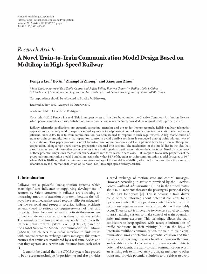
A Novel Train-to-Train Communication Model Design Based on Multihop in High-Speed RailwayPengyu Liu Bo Ai Zhangdui Zhong and Xiaojuan ZhouVolume 2012 Article ID 475492 9 pages
State Modelling of the Land Mobile Propagation Channel with Multiple Satellites Daniel ArndtAlexander Ihlow Albert Heuberger and Ernst EberleinVolume 2012 Article ID 625374 15 pages
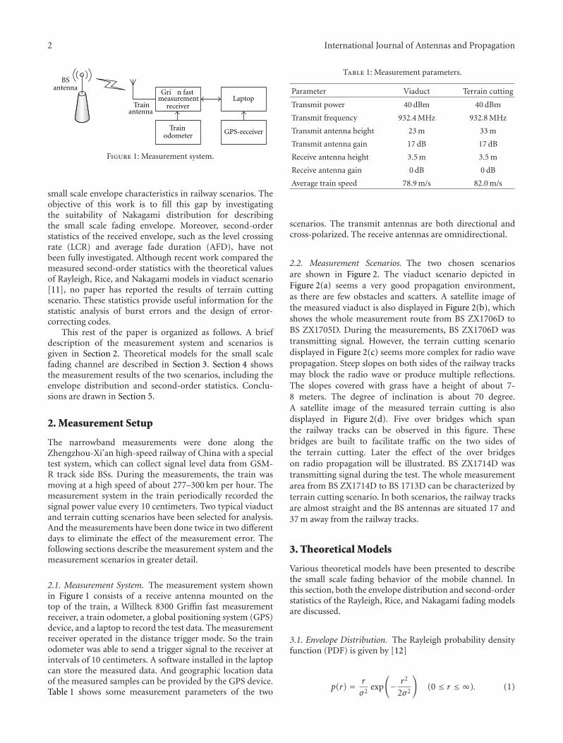
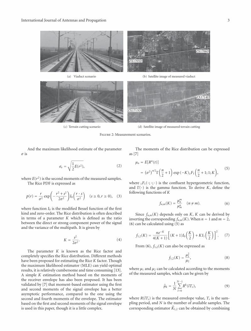
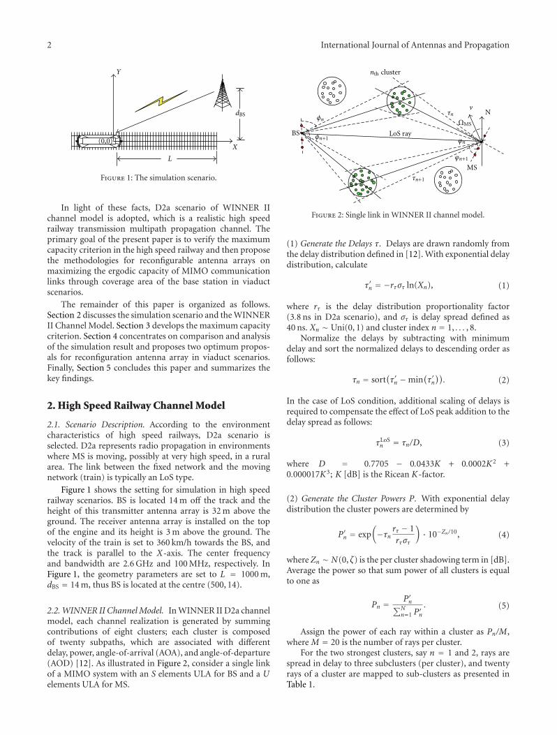
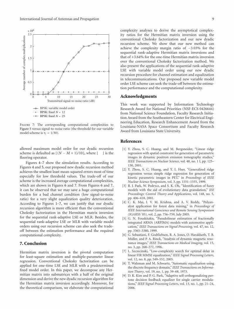
Fading Analysis for the High Speed Railway Viaduct and Terrain Cutting Scenarios Jinghui LuGang Zhu and Bo AiVolume 2012 Article ID 862945 9 pages
Impact of Ship Motions on Maritime Radio Links William Hubert Yvon-Marie Le Roux Michel Neyand Anne FlamandVolume 2012 Article ID 507094 6 pages
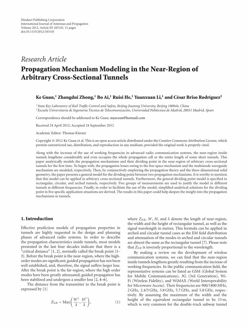
Propagation Mechanism Modeling in the Near-Region of Arbitrary Cross-Sectional Tunnels Ke GuanZhangdui Zhong Bo Ai Ruisi He Yuanxuan Li and Cesar Briso RodrıguezVolume 2012 Article ID 183145 11 pages
Statistical Modeling of Ultrawideband Body-Centric Wireless Channels Considering Room VolumeMiyuki Hirose Hironobu Yamamoto and Takehiko KobayashiVolume 2012 Article ID 150267 10 pages
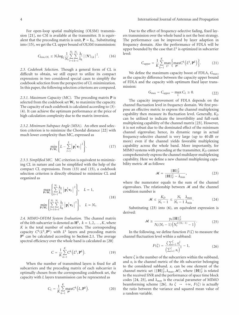
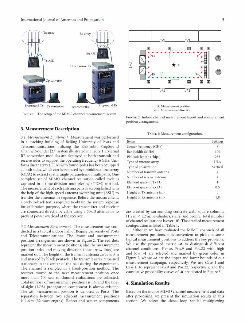
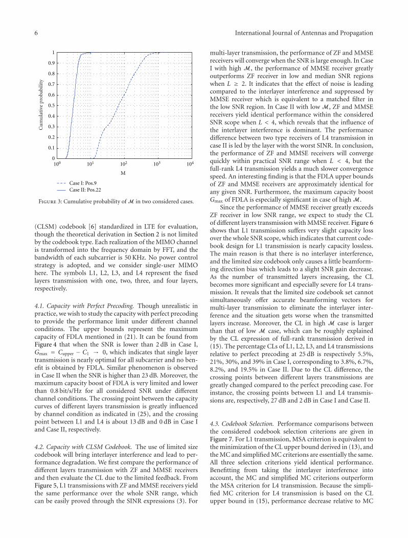
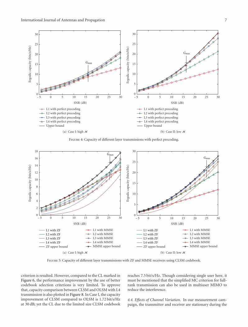
Performance Evaluation of Closed-Loop Spatial Multiplexing Codebook Based on Indoor MIMOChannel Measurement Junjun Gao Jianhua Zhang Yanwei Xiong Yanliang Sun and Xiaofeng TaoVolume 2012 Article ID 701985 10 pages
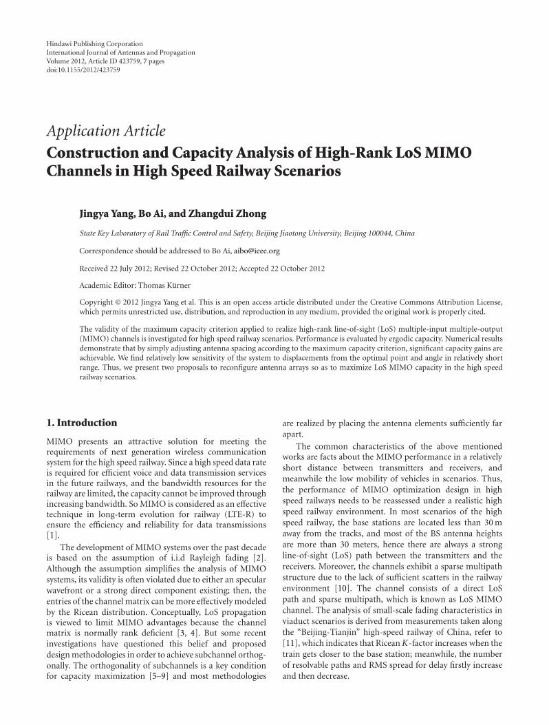
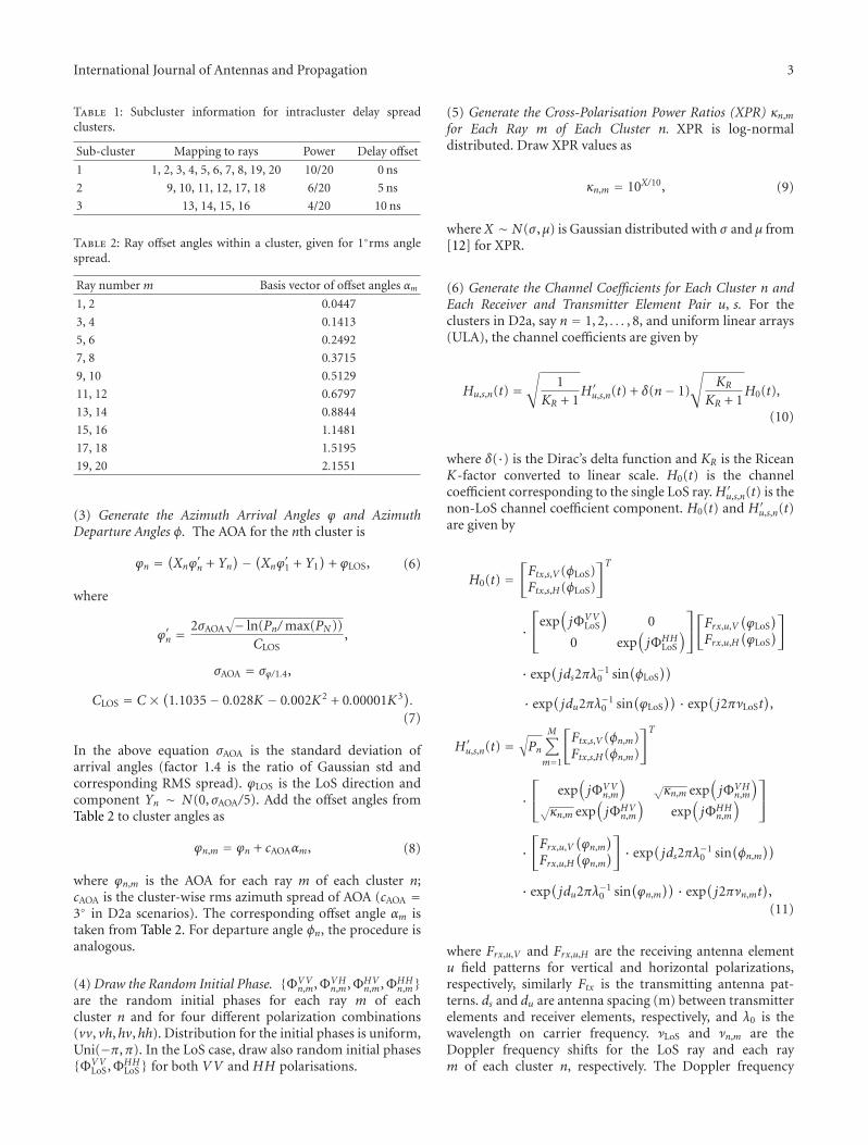
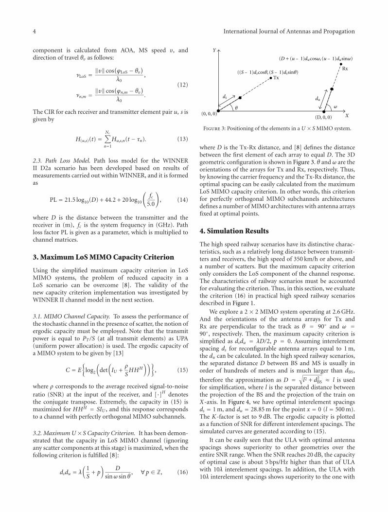
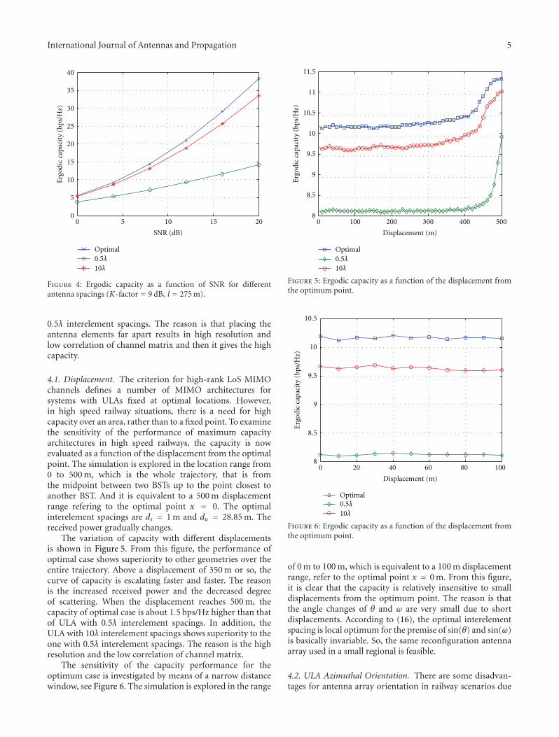
Construction and Capacity Analysis of High-Rank LoS MIMO Channels in High Speed RailwayScenarios Jingya Yang Bo Ai and Zhangdui ZhongVolume 2012 Article ID 423759 7 pages
Influence of Training Set Selection in Artificial Neural Network-Based Propagation Path LossPredictions Ignacio Fernandez Anitzine Juan Antonio Romo Argota and Fernado Perez FontanVolume 2012 Article ID 351487 7 pages
On the Statistical Properties of Nakagami-Hoyt Vehicle-to-Vehicle Fading Channel under NonisotropicScattering Muhammad Imran Akram and Asrar U H SheikhVolume 2012 Article ID 179378 12 pages
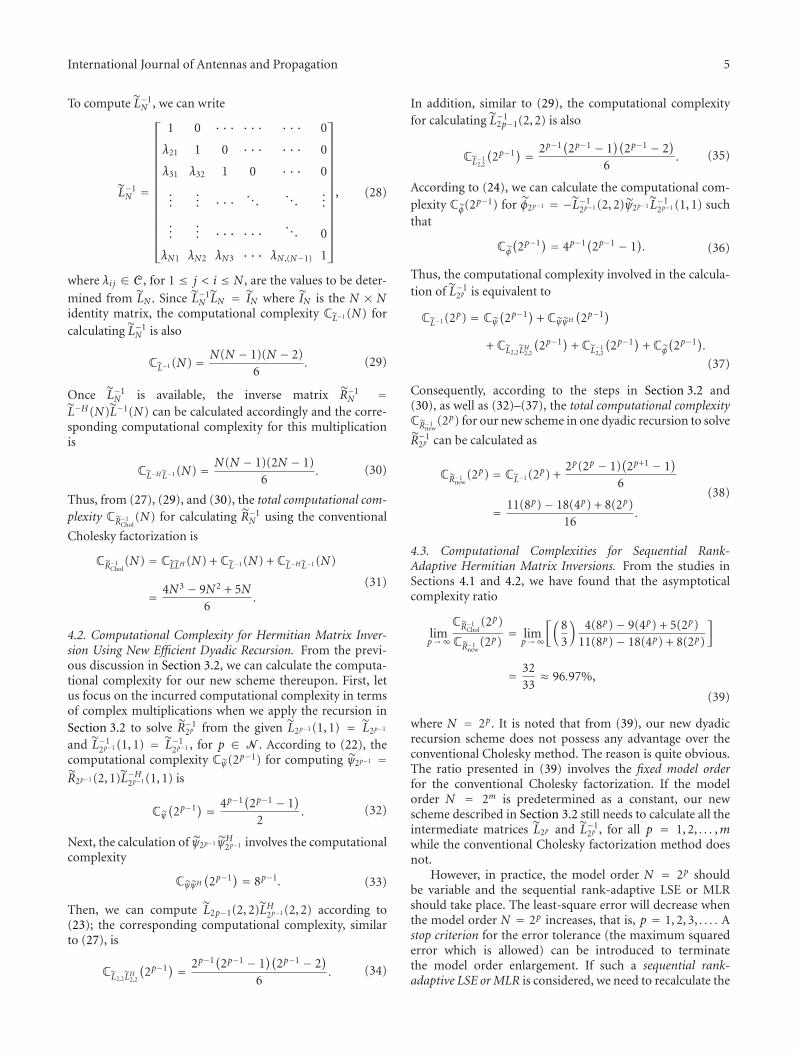
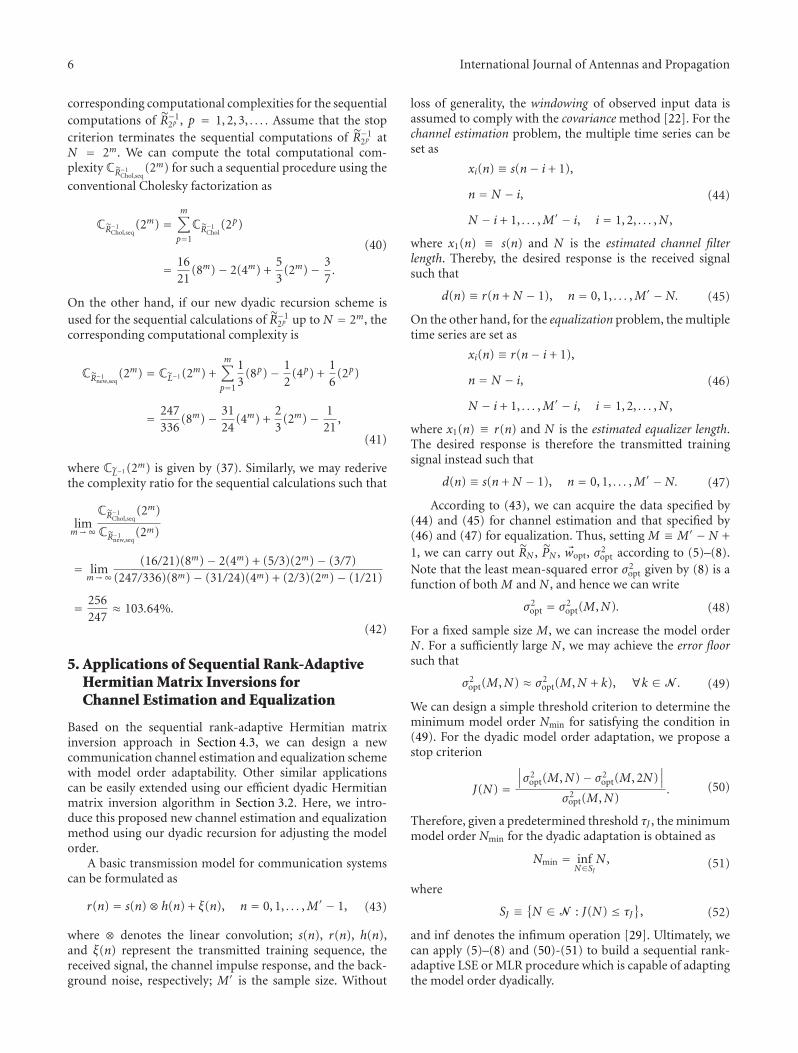
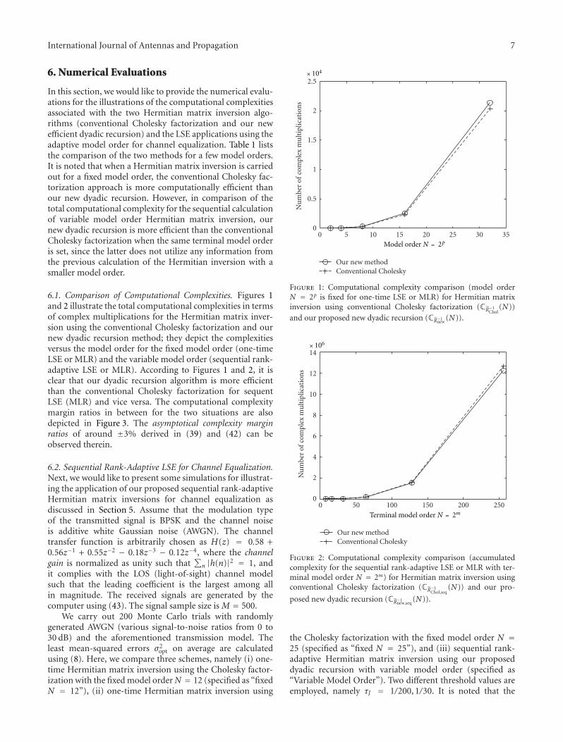
Efficient Rank-Adaptive Least-Square Estimation and Multiple-Parameter Linear Regression UsingNovel Dyadically Recursive Hermitian Matrix Inversion Hsiao-Chun Wu Shih Yu Chang Tho Le-Ngocand Yiyan WuVolume 2012 Article ID 891932 10 pages
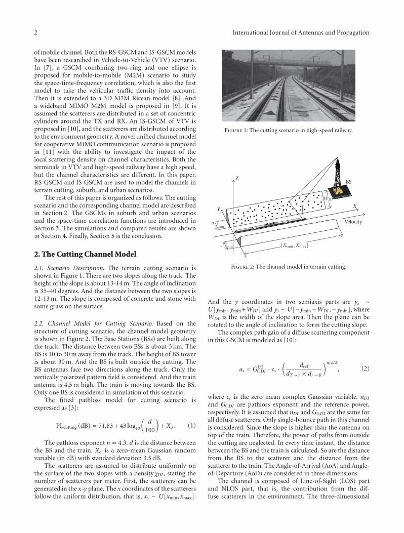
Geometry-Based Stochastic Modeling for MIMO Channel in High-Speed Mobile ScenarioBinghao Chen and Zhangdui ZhongVolume 2012 Article ID 184682 6 pages
Radio Wave Propagation Scene Partitioning for High-Speed Rails Bo Ai Ruisi He Zhangdui ZhongKe Guan Binghao Chen Pengyu Liu and Yuanxuan LiVolume 2012 Article ID 815232 7 pages
NECOP Propagation Experiment Rain-Rate Distributions Observations and Prediction ModelComparisons J S Ojo and S E FalodunVolume 2012 Article ID 913596 4 pages
Hindawi Publishing CorporationInternational Journal of Antennas and PropagationVolume 2013 Article ID 835160 3 pageshttpdxdoiorg1011552013835160
Editorial
Radio Wave Propagation and Wireless Channel Modeling
Ai Bo1 Thomas Kuumlrner2 Ceacutesar Briso Rodriacuteguez3 and Hsiao-Chun Wu4
1 State Key Laboratory of Rail Traffic Control and Safety Beijing Jiaotong University Beijing 100044 China2 Technische Universitat Braunschweig Braunschweig 38106 Germany3Universidad Politecnica de Madrid Madrid 28031 Spain4 Louisiana State University LA 70803 USA
Correspondence should be addressed to Ai Bo aiboieeeorg
Received 25 November 2012 Accepted 25 November 2012
Copyright copy 2013 Ai Bo et al This is an open access article distributed under the Creative Commons Attribution License whichpermits unrestricted use distribution and reproduction in any medium provided the original work is properly cited
Mechanisms about radio wave propagation are the basis forwireless channel modeling Typical wireless channel modelsfor typical scenarios are of great importance to the physicallayer techniques such as synchronization channel estima-tion and equalization Nowadays many channel modelsconcerned with either large-scale modeling and small-scalefast fading models have been established However withthe development of some new techniques such as mul-tiuser MIMO systems vehicle-to-vehicle technique wirelessrelay technique and short-distance or short-range techniquenovel wireless channel models should be developed to caterfor these new applications As for this special issue wecordially invite some researchers to contribute papers thatwill stimulate the continuing efforts to understand the mech-anisms about radio wave propagations and wireless channelmodels under variant scenarios This special issue providesthe state-of-the-art research in mobile wireless channels
As we know scene partitioning is the premise and basisfor wireless channel modeling The paper titled ldquoRadio wavepropagation scene partitioning for high-speed railsrdquo discussesthe scene partitioning for high-speed rail (HSR) scenariosBased on the measurements along HSR lines with 300 kmhoperation speed in China the authors partitioned the HSRscene into twelve scenarios Further work based on theoret-ical analysis of radio wave propagation mechanisms such asreflection and diffraction may lead to develop the standardof radio wave propagation scene partitioning for HSR
The paper ldquoQuantification of scenario distance withingeneric WINNER channel modelrdquo deals with the topic on thescenario comparisons on the basis of the fundamental theorythat a generic WINNER model uses the same set of parame-ters for representing different scenarios It approximates the
WINNER scenarios with multivariate normal distributionsand then uses the mean Kullback-Leibler divergence toquantify the divergence The results show that the WINNERscenario groups (A B C D) or propagation classes (LoSNLoS) do not necessarily ensure minimum separation withinthe groupsclasses The computation of the divergence of theactual measurements and WINNER scenarios confirms thatthe parameters of the C2 scenario in WINNER series area proper reference for a large variety of urban macrocellenvironments
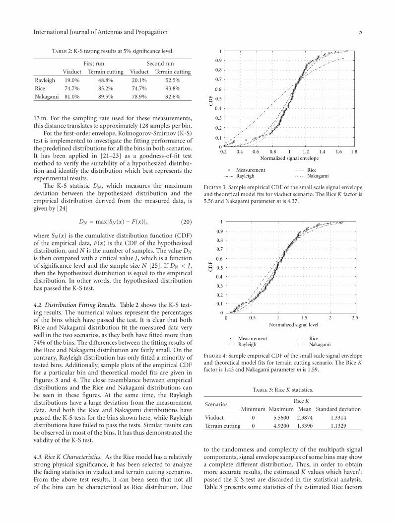
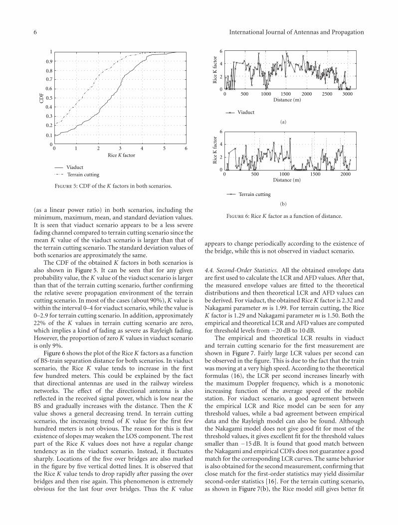
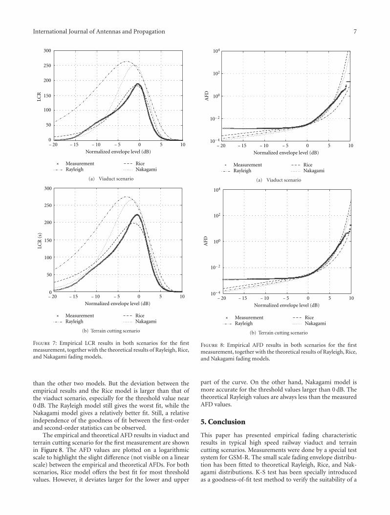
The paper ldquoFading analysis for the high speed railwayviaduct and terrain cutting scenariosrdquo provides a good under-standing of fading characteristics in HSR environment basedon the measurements taken in both high-speed viaductand terrain cutting scenarios using track side base stationsKolmogorov-Smirnov (K-S) test has been first introducedin the statistical analysis to find out the most appropriatemodel for the small-scale fading envelope Some importantconclusions are drawn though both Rice and Nakagamidistributions provide a good fit to the first-order envelopedata in both scenarios only the Rice model generally fitsthe second-order statistics data accurately For the viaductscenario higher Rice K factor can be observed The changetendency of the K factor as a function of distance in the twoscenarios is completely different
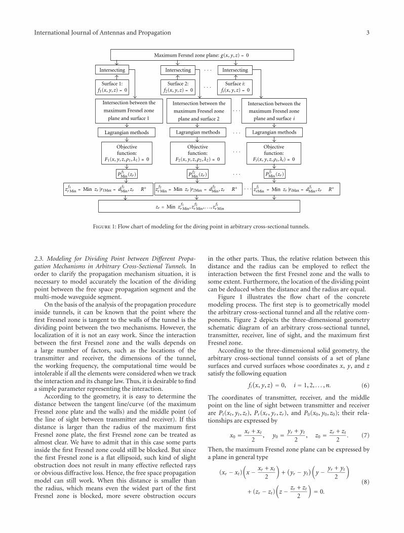
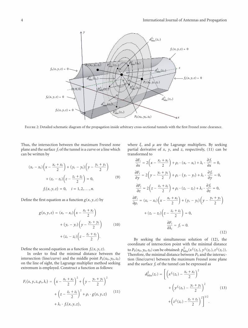
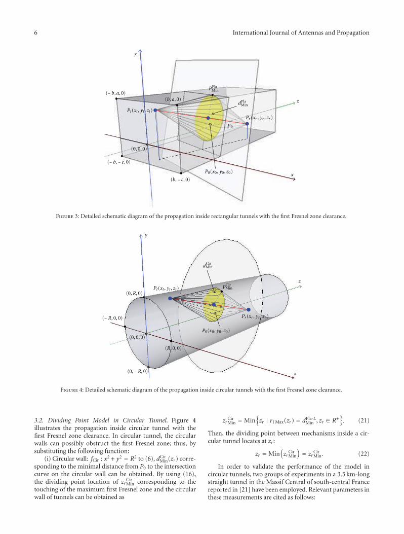
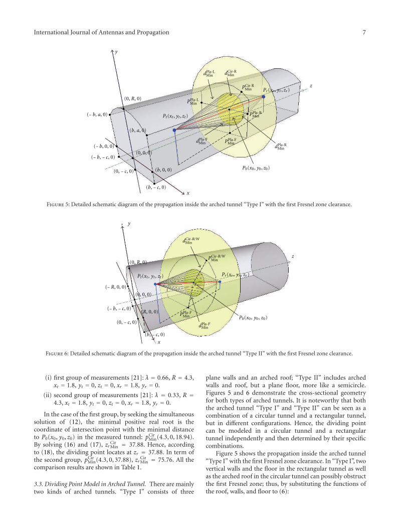
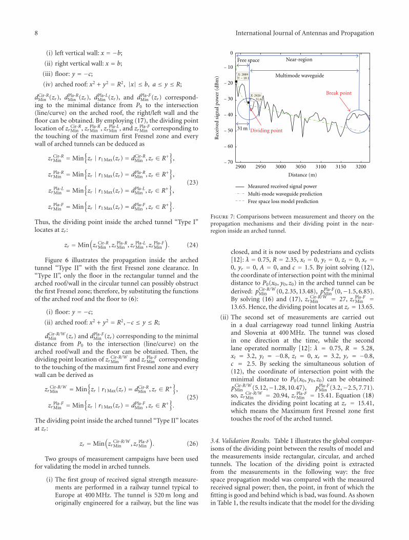
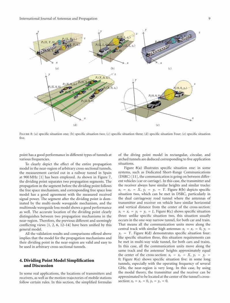
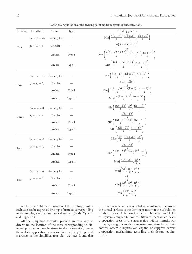
The paper ldquoPropagation mechanism modeling in the near-region of arbitrary cross-sectional tunnelsrdquo talks about themodeling of the propagation mechanisms and their dividingpoint in the near-region of arbitrary cross-sectional tunnelsBy conjunctively employing the propagation theory and thethree-dimensional solid geometry it presents a general modelfor the dividing point between two propagation mechanisms
2 International Journal of Antennas and Propagation
Furthermore the general dividing point model is specifiedin rectangular circular and arched tunnels respectively Fivegroups of measurements are used to justify the model indifferent tunnels at different frequencies The results couldhelp to deepen the insight into the propagation mechanismsin tunnels
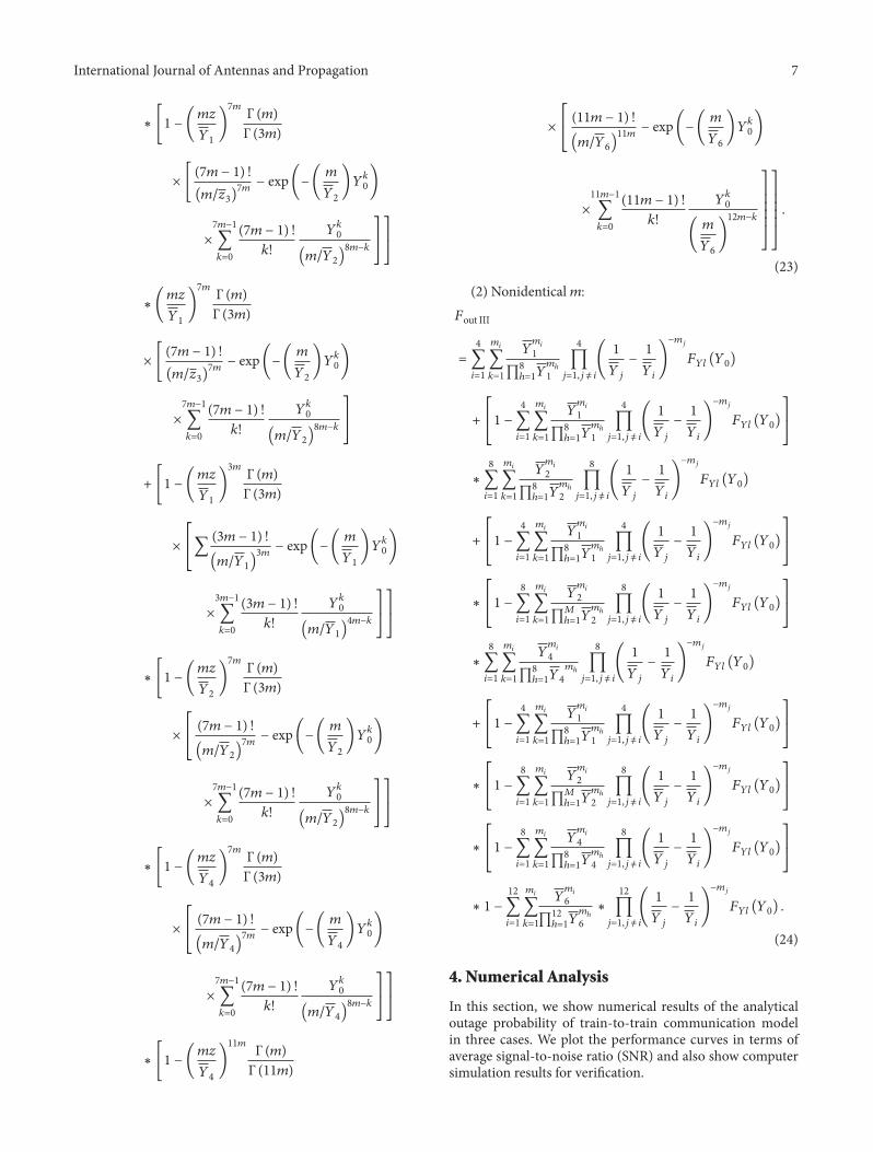
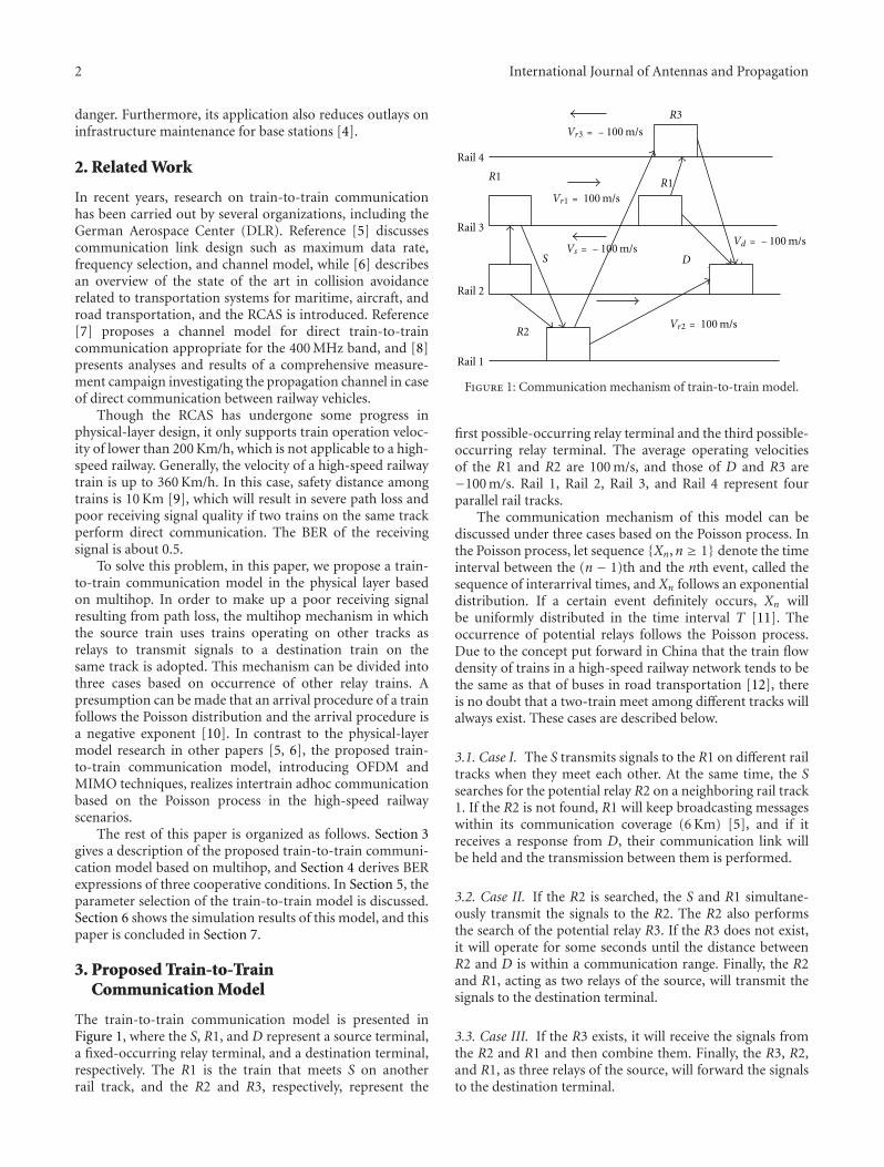
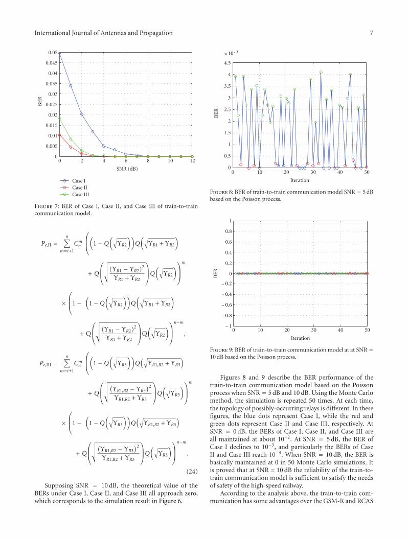
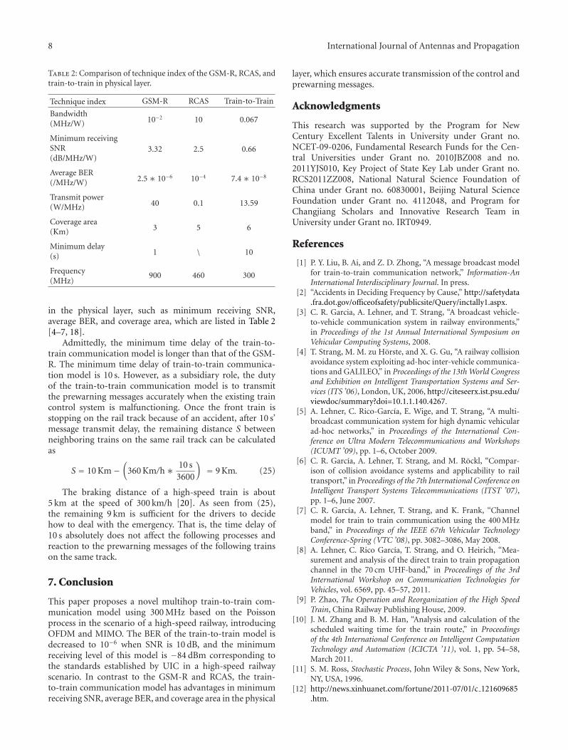
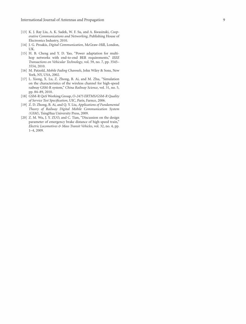
A key characteristic of train-to-train (T2T) communi-cation a recently proposed novel technique for HSR is toavoid accidents conducted among trains without any aid ofinfrastructure The paper ldquoA novel train-to-train communica-tion model design based on multihop in high-speed railwayrdquoprovides a novel T2T communication model in a physicallayer based on multihop and cooperation technique Themechanism of this model lies in the idea that a sourcetrain uses trains on other tracks as relays to transmit signalsto destination train on the same track The paper titledldquoOutage analysis of train-to-train communication model overNakagami-m channel in high-speed railwayrdquo analyzes the end-to-end outage performance of T2T communication model inHSR over independent identical and nonidentical Nakagami-m channels It presents a novel closed form for the sum ofsquared independent Nakagami-m variates and then derivesan expression for the outage probability of the identicaland nonidentical Nakagami-m channels Numerical analysisindicates that the derived analytical results are reasonable andthe outage performance is better over Nakagami-m channelin HSR scenarios
The above-mentioned papers are for HSR communica-tion wireless channel models There are also some papersdealing with the channel models for satellites ships humanbodies and vehicle-to-vehicle communications
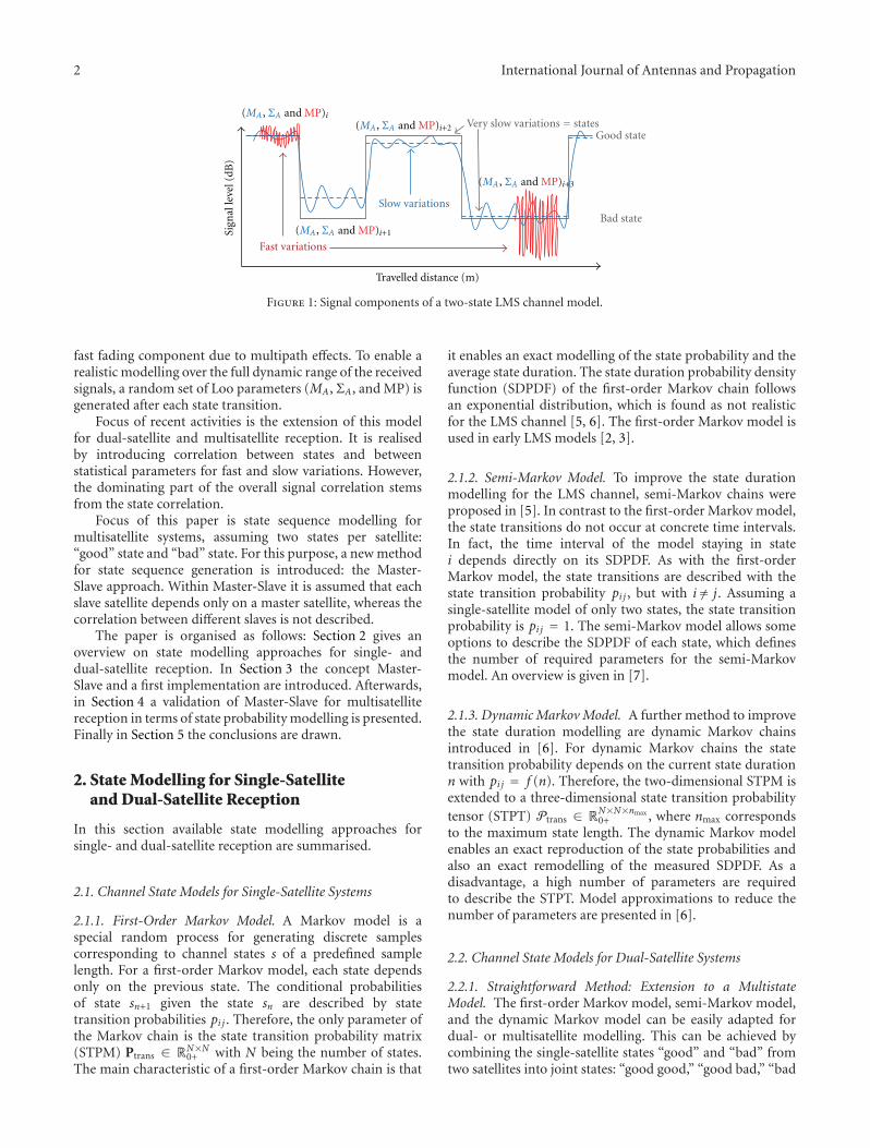
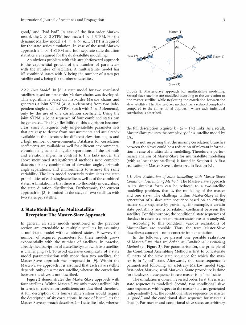
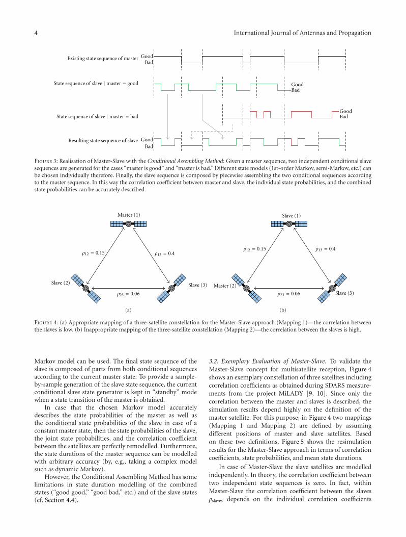
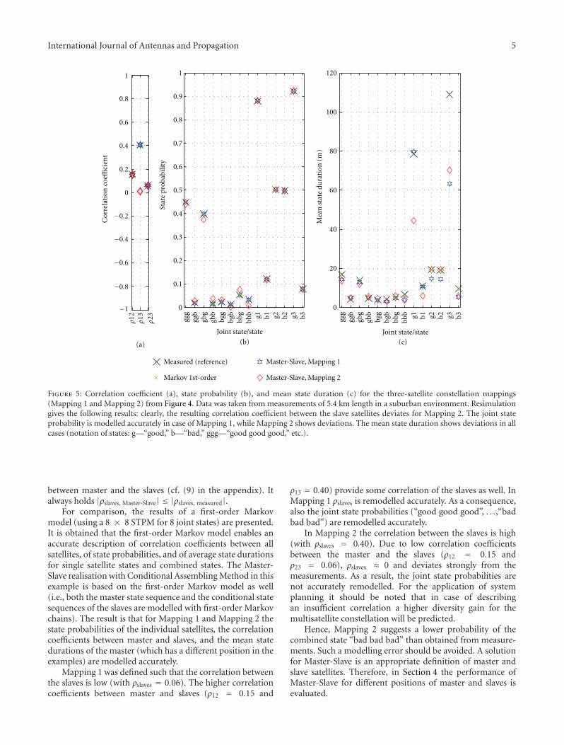
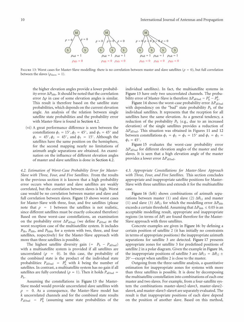
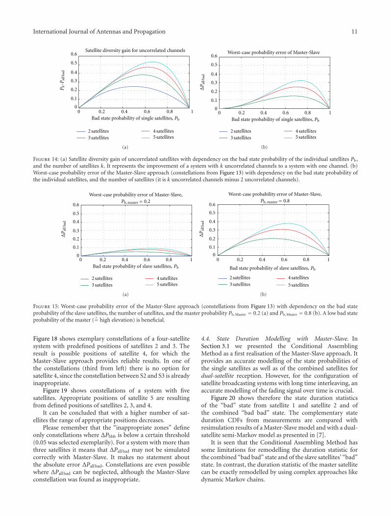
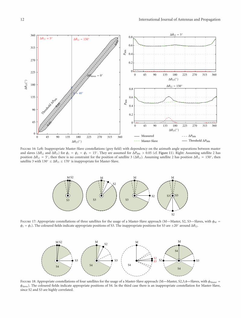
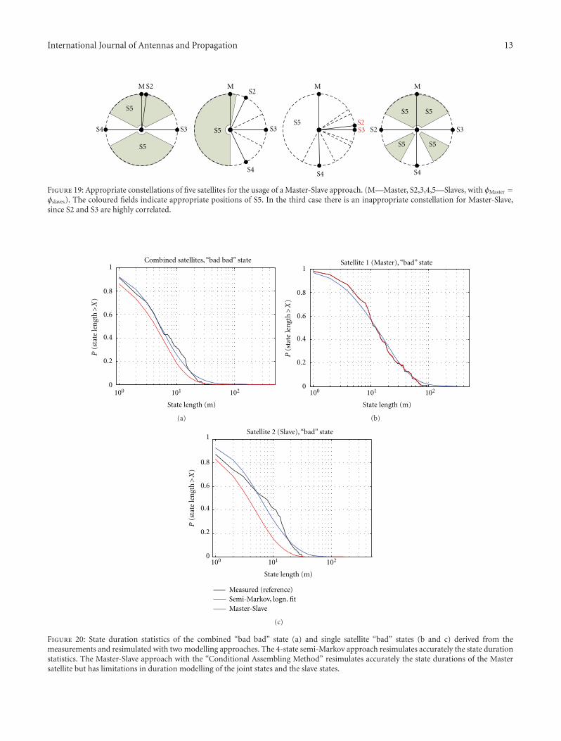
The paper ldquoState modeling of the land mobile propagationchannel with multiple satellitesrdquo evaluates a novel approachfor multisatellite state modeling the Master-Slave approachand its corresponding realization method named ConditionalAssembling Method The primary concept is that slavesatellites are modeled according to an existing master statesequence whereas the correlation between multiple slavesis omitted For modeling two satellites (one master and oneslave) the ldquoConditional Assembling Methodrdquo enables anaccurate resimulation of the correlation coefficient betweenthe satellites the single satellite state probabilities andthe combined state probabilities of master and slave Theprobability of the ldquoall bad-rdquo state resulting from master-slave is compared with an analytically estimated ldquoall bad-rdquostate probability from measurements Master-slave has a highprobability error in case of a high correlation between theslave satellites Furthermore a master satellite with a highelevation provides a lower probability error compared to amaster with low elevation
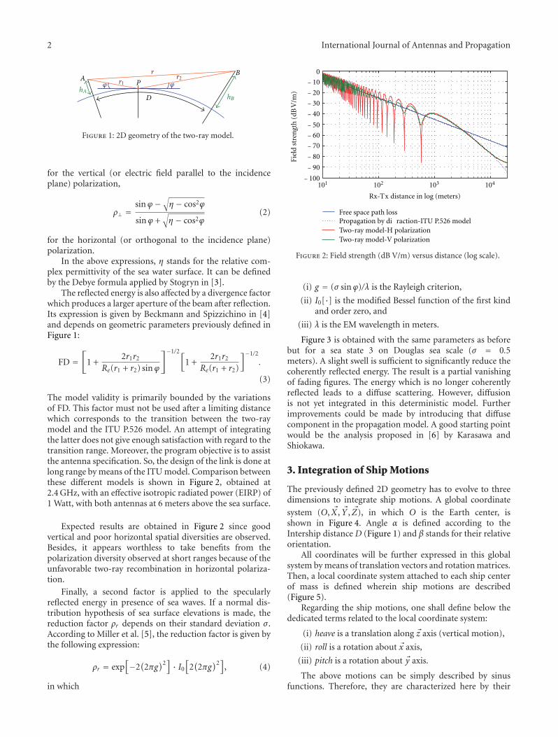
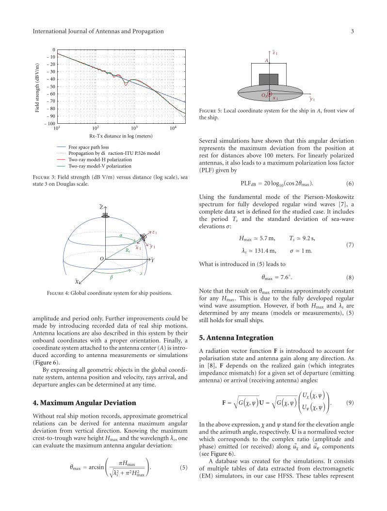
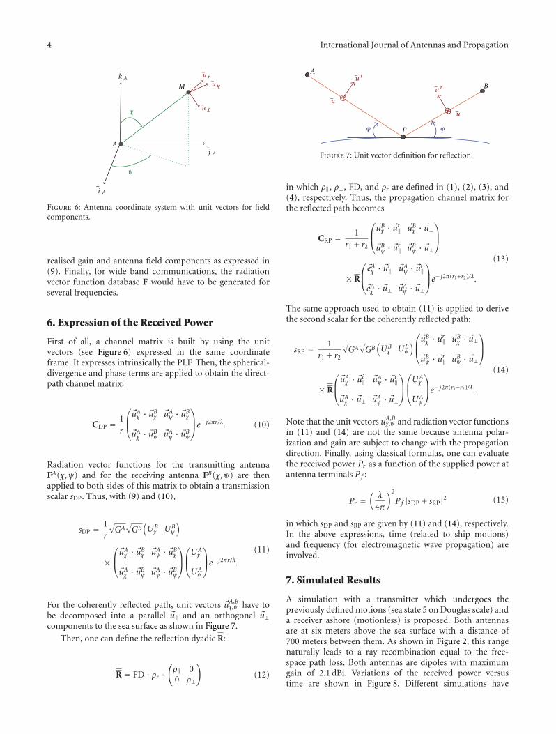
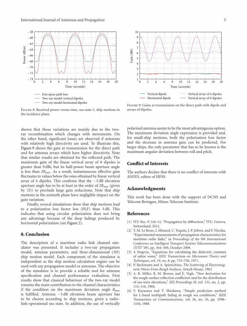
The improvement of maritime radio links often requiresan increase of emitted power or receiver sensitivity Anotherway is to replace the poor antenna gains of traditionalsurface ship whips by novel antenna structures with directiveproperties The paper ldquoImpact of ship motions on maritimeradio linksrdquo developed a tool for modeling the impact ofship motions on the antenna structures The tool includes adeterministic two-ray model for radio-wave propagation overthe sea surface
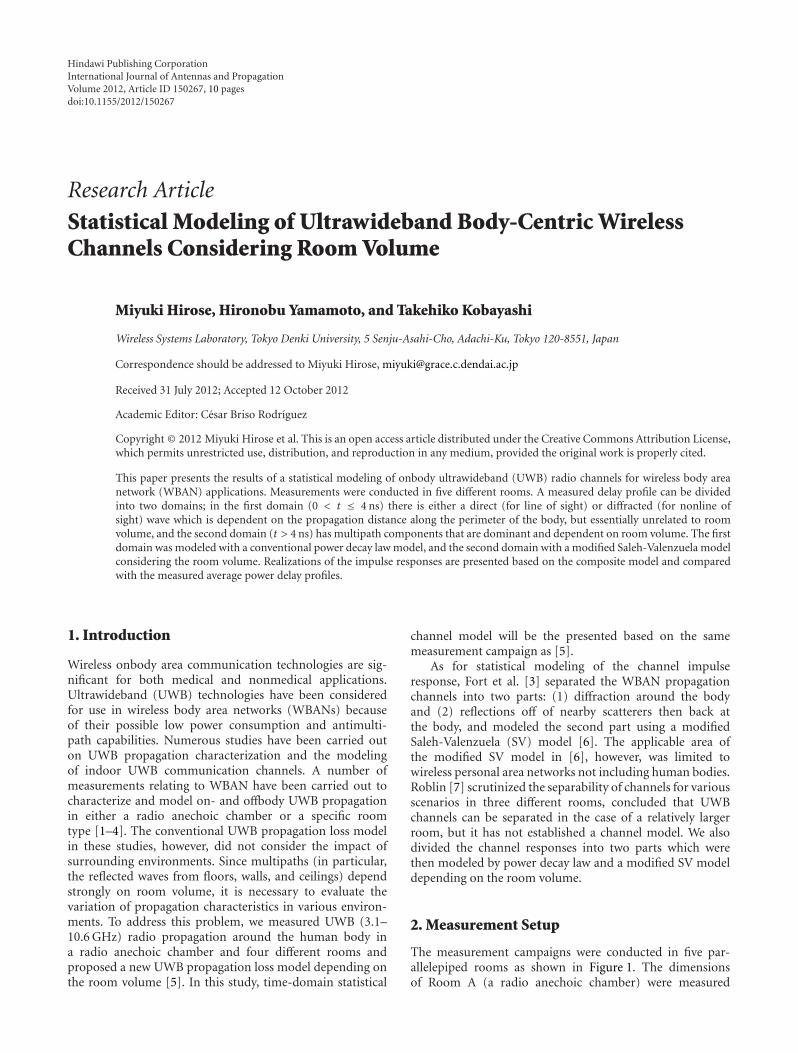
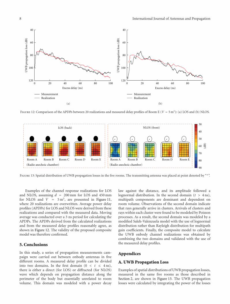
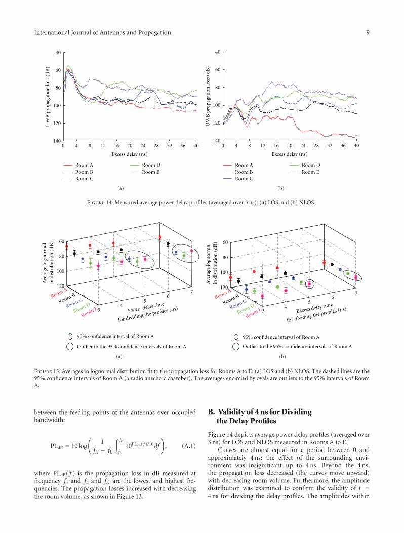
The paper ldquoStatistical modeling of ultrawideband body-centric wireless channels considering room volumerdquo presentsthe results of a statistical modeling of on-body ultrawide-band (UWB) radio channels for wireless body area network
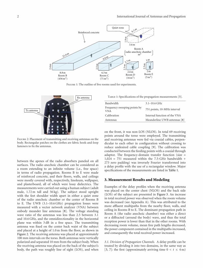
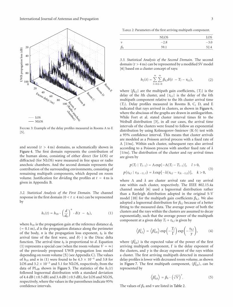
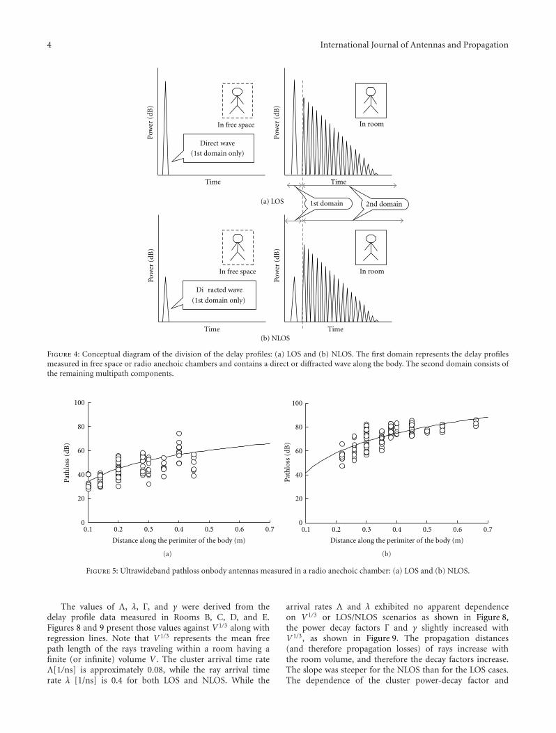
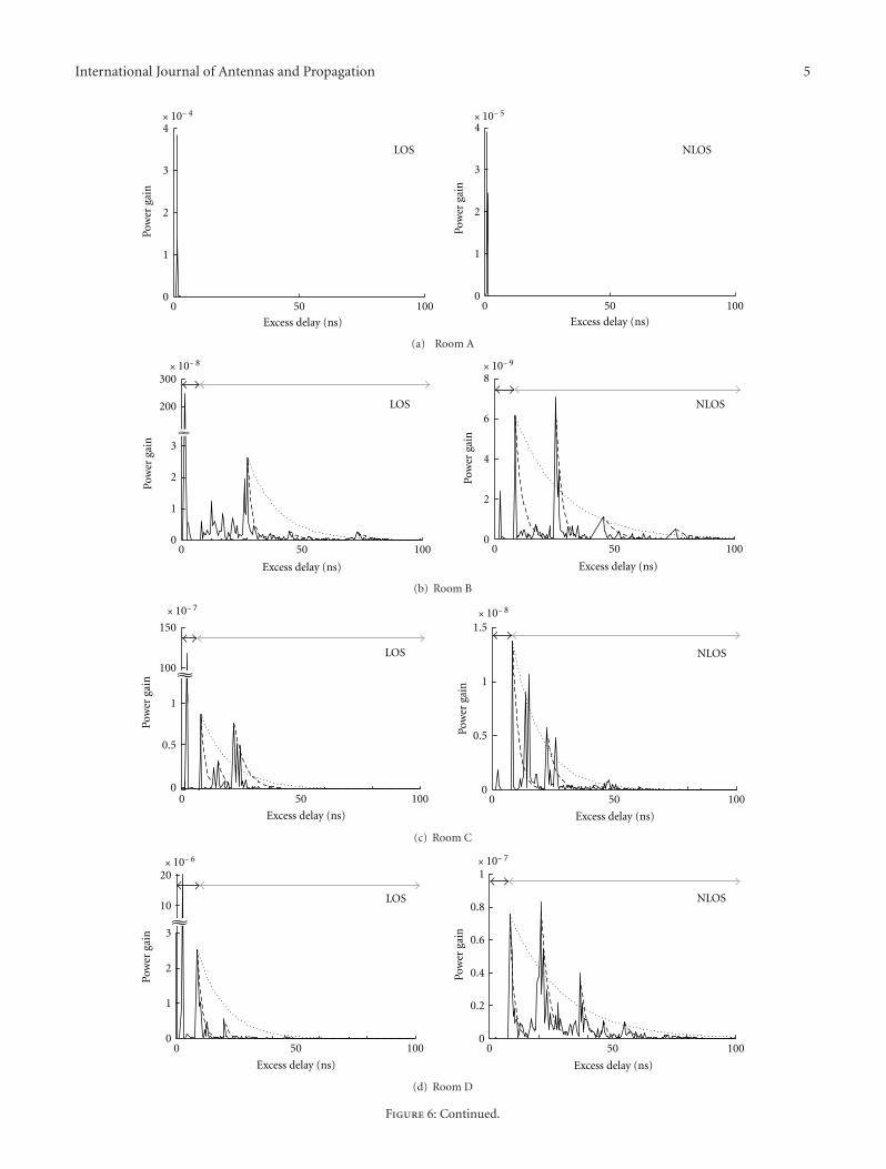
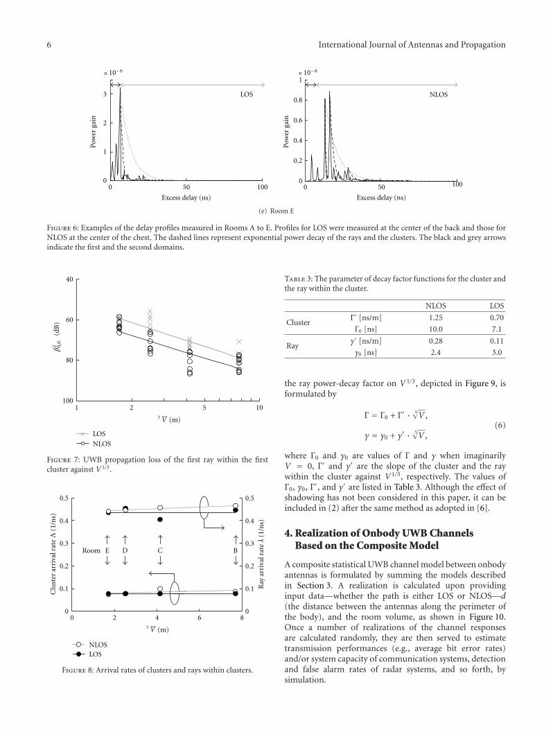
(WBAN) applications A measured delay profile can bedivided into two domains in the first domain there is eithera direct (for line of sight) or diffracted (for nonline of sight)wave which is dependent on the propagation distance alongthe perimeter of the body but essentially unrelated to roomvolume and the second domain has multipath componentsthat are dominant and dependent on room volume Thefirst domain was modeled with a conventional power decaylaw model and the second domain with a modified Saleh-Valenzuela model considering the room volume Realizationsof the impulse responses are presented based on the compos-ite model and compared with the measured average powerdelay profiles
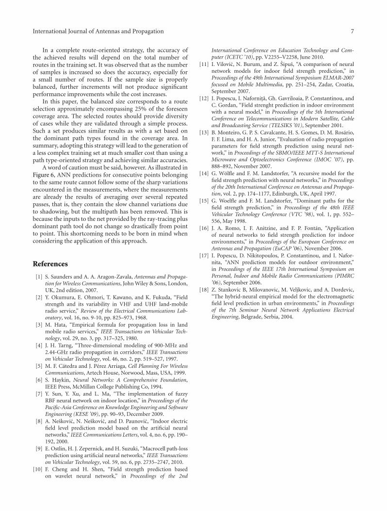
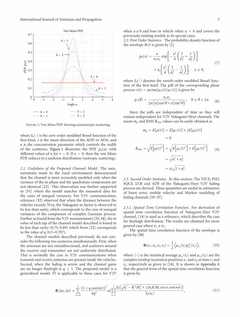
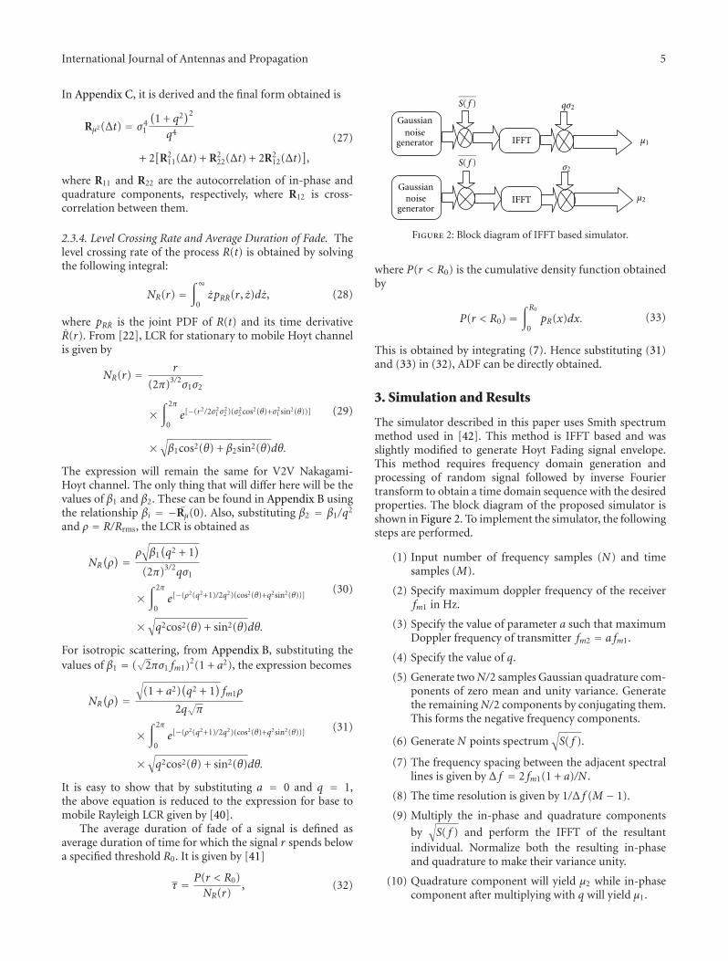
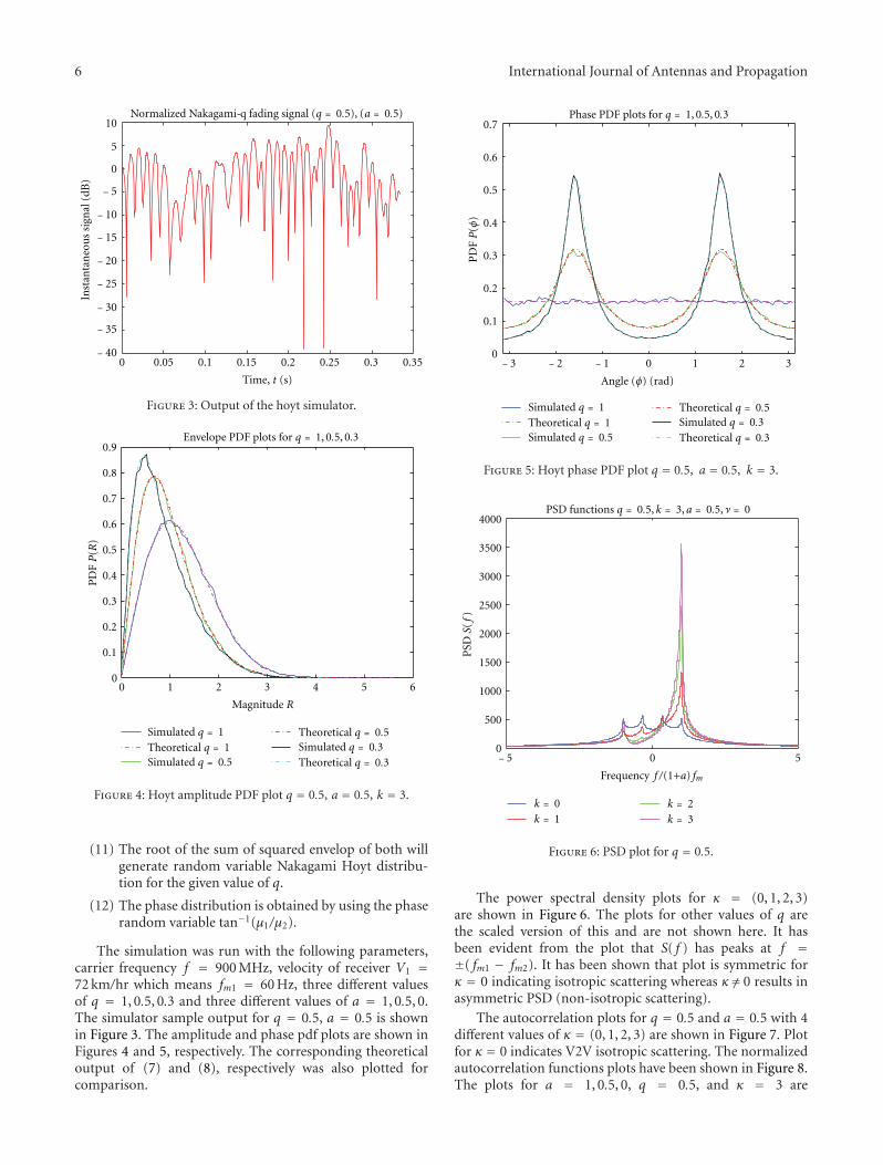
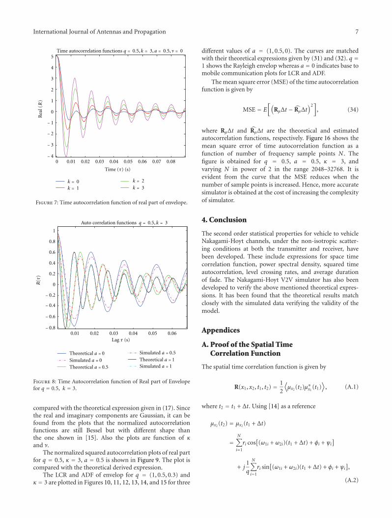
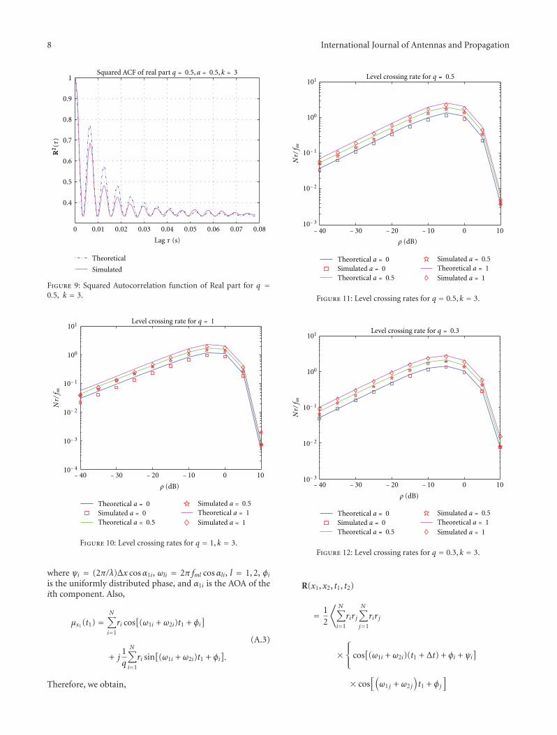
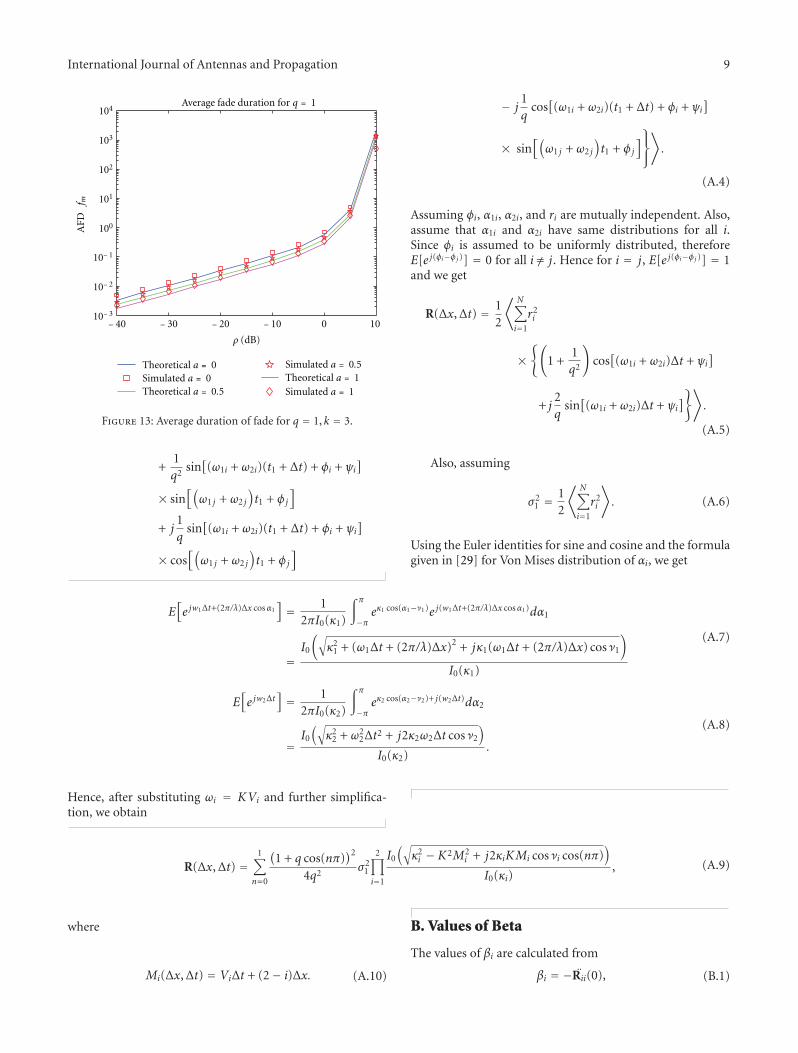
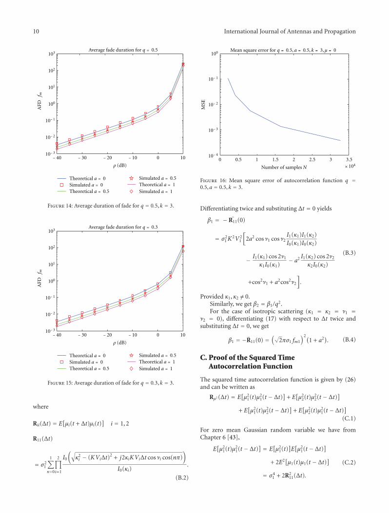
The paper titled ldquoOn the statistical properties of Nakagami-hoyt vehicle-to-vehicle fading channel under nonisotropic scat-teringrdquo argues the statistical properties of vehicle-to-vehicleNakagami-Hoyt (Nakagami-q) channel model under non-isotropic condition The spatial-time correlation function(STCF) the power spectral density (PSD) squared timeautocorrelation function (SQCF) level crossing rate (LCR)and the average duration of fade (ADF) of the Nakagami-Hoyt channel have been derived under the assumptionthat both the transmitter and receiver are nonstationarywith nonomnidirectional antennas A simulator utilizing theinverse-fast-fourier-transform- (IFFT-) based computationmethod is designed for the model
The paper ldquoNECOP propagation experiment rain-ratedistributions observations and prediction model comparisonsrdquotalks about the empirical distribution functions for the eval-uation of rain-rate based on the observed data The empiricaldistribution functions were compared with cumulative dis-tribution functions generated using four different rain-ratedistribution models It is found that although each of themodels shows similar qualitative features at lower exceedanceof time the characteristics at higher time percentages showquantitative difference from the experimental data except theimproved version of Moupfouma model The results furthershow that the rain-fall rate and the microwave propagationcharacteristics in the observed region are out of accord withInternational Telecommunication Union predictions Thisinformation is vital for predicting rain fading cumulativeprobability distributions
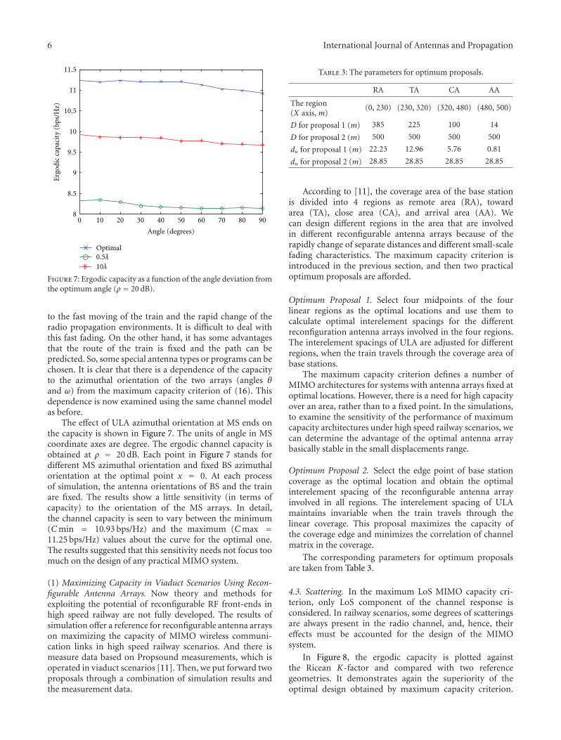
The paper ldquoInfluence of training set selection in artificialneural network-based propagation path loss predictionsrdquo uti-lizes the artificial neural networks (ANNs) and ray-tracingtechnique for predicting the received powerpath loss inboth outdoor and indoor links A complete description ofthe process for creating and training an ANN-based modelis presented with special emphasis on the training process
The optimum selection of the training set is discussed Aquantitative analysis based on results from two narrowbandmeasurement campaigns is also presented
The following fours papers are related with multi-inputand multioutput (MIMO) techniques The paper ldquoA tradeoff
International Journal of Antennas and Propagation 3
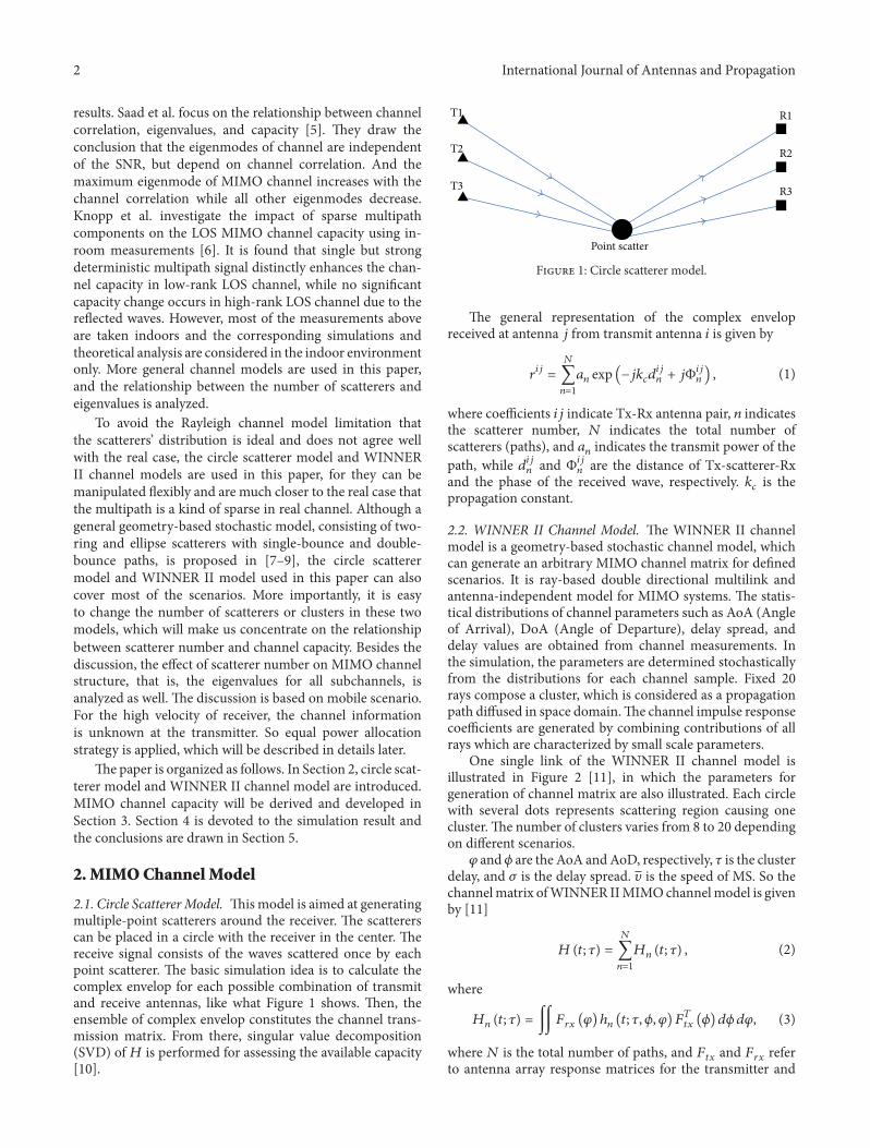
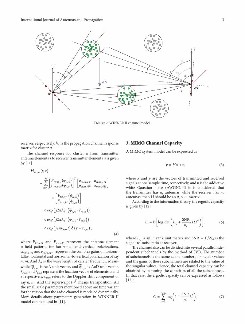
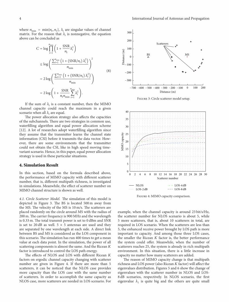
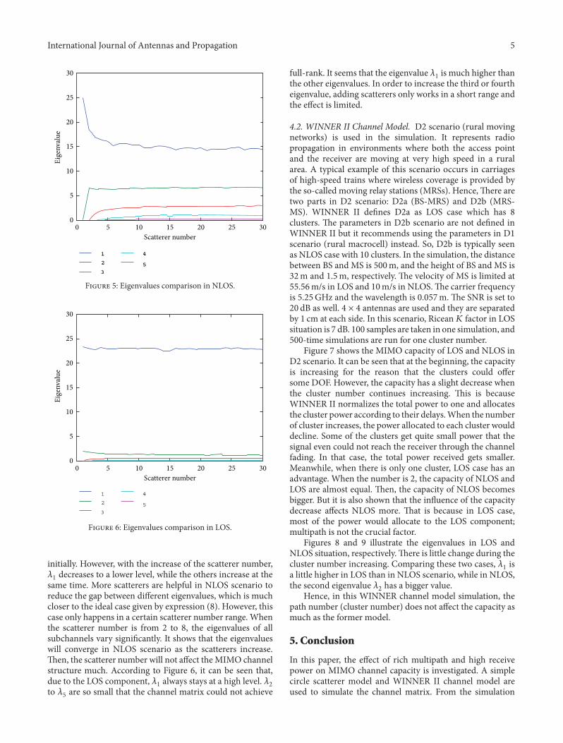
between rich multipath and high receive power in MIMOcapacityrdquo presents a discussion of rich multipath (in NLOS) orsignal-to-noise ratio (SNR) (usually in LOS) effects on MIMOchannel capacity It is investigated by performing simulationsusing simple circle scatterer and WINNER II channel modelThe simulation results show that these two factors behavedifferently as the channel conditions vary When the scatterernumber in channel is low the high receive SNR is moreimportant than capacity The multipath richness will get theupper bound when the scatterer number is beyond a certainthreshold However the channel capacity will not changemuch as the scatterers continue to increase
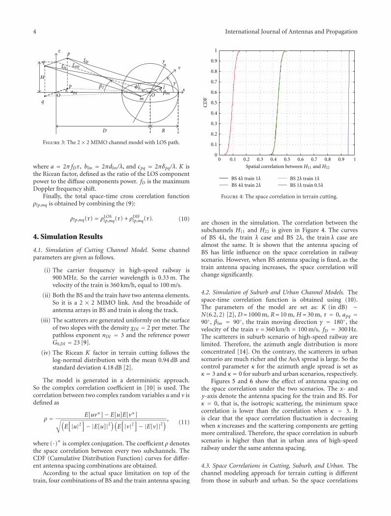
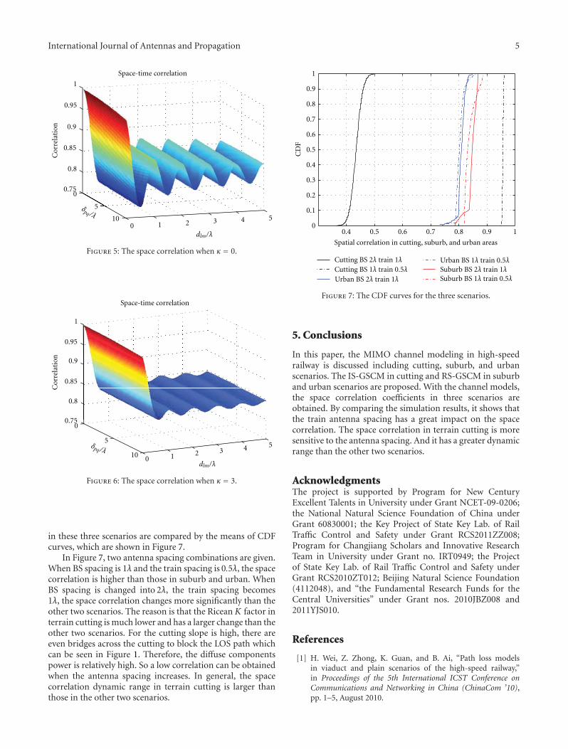
The paper ldquoConstruction and capacity analysis of high-rank LoS MIMO channels in high speed railway scenariosrdquotalks about the validity of the maximum capacity criterionapplied to realize high-rank LoS MIMO channels for HSRscenarios Performance is evaluated by ergodic capacityNumerical results demonstrate that by simply adjustingantenna spacing according to the maximum capacity crite-rion significant capacity gains are achievable Two proposalsare presented to reconfigure antenna arrays so as to maxi-mize LoS MIMO capacity in the HSR scenarios The paperldquoGeometry-based stochastic modeling for MIMO channel inhigh-speed mobile scenariordquo discusses the geometry-basedstochastic channel models for the terrain cutting suburband urban scenarios in HSR The space time correlationfunctions in analytical form are obtained in suburb andurban scenarios The comparisons of the space correlationcharacteristics under three scenarios are made
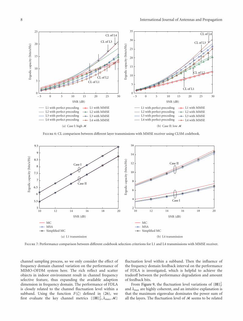
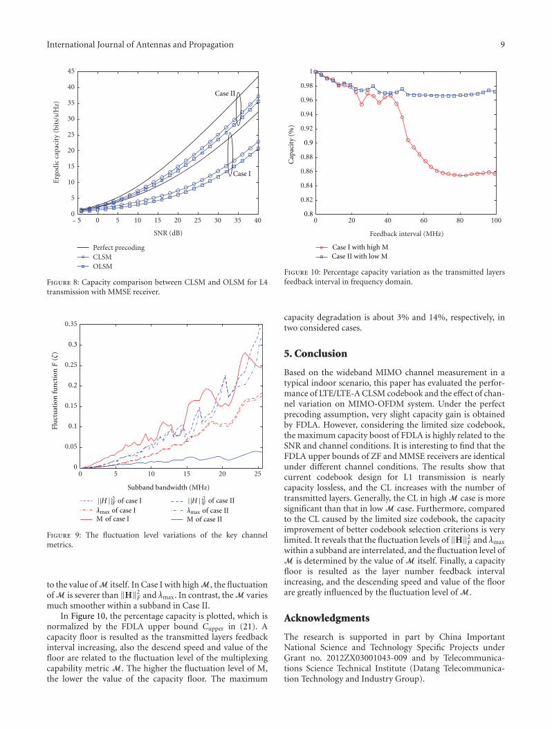
The paper ldquoPerformance evaluation of closed-loop spatialmultiplexing codebook based on indoor MIMO channel mea-surementrdquo discusses closed-loop MIMO technique standard-ized for long-term evolution (LTE) system Based on thewideband MIMO channel measurement in a typical indoorscenario capacity loss (CL) of the limited size codebookrelative to perfect precoding is studied in two extremechannel conditions The results show that current codebookdesign for single-layer transmission is nearly capacity losslessand the CL will increase with the number of transmittedlayers Furthermore the capacity improvement of bettercodebook selection criterions is very limited compared to CLTo survey the effect of frequency domain channel variation onMIMO-OFDM system a function is defined to measure thefluctuation levels of the key channel metrics within a subbandand to reveal the inherent relationship between them
Ai BoThomas Kurner
Cesar Briso RodrıguezHsiao-Chun Wu
Hindawi Publishing CorporationInternational Journal of Antennas and PropagationVolume 2013 Article ID 176704 17 pageshttpdxdoiorg1011552013176704
Research Article
Quantification of Scenario Distance withinGeneric WINNER Channel Model
Milan NarandDiT1 Christian Schneider2 Wim Kotterman3 and Reiner S Thomauml2
1 Department for Power Electronic and Communication Engineering Faculty of Technical SciencesTrg D Obradovica 6 2100 Novi Sad Serbia
2 Electronic Measurement Research Lab Ilmenau University of Technology PSF 100565 98684 Ilmenau Germany3Digital Broadcasting Research Laboratory Ilmenau University of Technology PSF 100565 98684 Ilmenau Germany
Correspondence should be addressed to Milan Narandzic orangeunsacrs
Received 27 July 2012 Revised 29 October 2012 Accepted 1 November 2012
Academic Editor Ai Bo
Copyright copy 2013 Milan Narandzic et al This is an open access article distributed under the Creative Commons AttributionLicense which permits unrestricted use distribution and reproduction in any medium provided the original work is properlycited
Starting from the premise that stochastic properties of a radio environment can be abstracted by defining scenarios a genericMIMO channel model is built by the WINNER project The parameter space of the WINNER model is among others describedby normal probability distributions and correlation coefficients that provide a suitable space for scenario comparison Thepossibility to quantify the distance between reference scenarios and measurements enables objective comparison and classificationof measurements into scenario classes In this paper we approximate the WINNER scenarios with multivariate normal distributionsand then use the mean Kullback-Leibler divergence to quantify their divergence The results show that the WINNER scenariogroups (A B C and D) or propagation classes (LoS OLoS and NLoS) do not necessarily ensure minimum separation withinthe groupsclasses Instead the following grouping minimizes intragroup distances (i) indoor-to-outdoor and outdoor-to-indoorscenarios (A2 B4 and C4) (ii) macrocell configurations for suburban urban and rural scenarios (C1 C2 and D1) and (iii)indoorhotspotmicrocellular scenarios (A1 B3 and B1) The computation of the divergence between Ilmenau and Dresdenmeasurements and WINNER scenarios confirms that the parameters of the C2 scenario are a proper reference for a large varietyof urban macrocell environments
1 Introduction
In order to maximize transmission efficiency wireless com-munication systems are forced to exploit the spatial andtemporal dimensions of the radio channel to the full Thedesign and performance analysis of such system requires thechannel model to reflect all relevant propagation aspectswhich imposes serious constraints on the minimal complex-ity of the model
This paper concentrates on the class of geometry-basedstochastic channel models (GSCMs) that offer good trade-off between complexity and performance (realism) Thesemodels deal with physical ray propagation and thereforeimplicitly or explicitly include the geometry of the propaga-tion environment The flexible structure of GSCMs enablesthe representation of different propagation environments bysimple adjustment of model parameters which is referred to
as generic property The generic models introduce abstractclasses called scenarios that act as stochastic equivalentsfor many similar radio environments As discussed in [1]these scenarios are not necessarily distinguished by thequantification of parametric space but they represent aconvenient terminology to designate typical deployment andpropagation conditions From history it was COST207 [2]that started classifying environments based on the type of dis-persion (delay spread and delay window) so some intuitiveconsideration of the (rather limited) parameter space wasinvolved But these types of differences have (almost) neverbeen sought later on when defining new scenarios especiallyfollowing deployment schemes
Nowadays we can distinguish between two majorclasses of generic models COST 2592732100 ([3ndash5] resp)and 3GPP SCM [6]WINNER [7 8] The first one definesspatial regions where interacting objects become ldquovisiblerdquo
2 International Journal of Antennas and Propagation
that is contributing to the total received field The secondclass offers an abstraction of the environment in parametricspace by using delay and angular spreads cross-polarizationshadowing119870-factor and so forth These generic models havebeen made by joint effort of many institutions otherwiseprovision of parameters for different scenarios would beunattainable Despite different model structures significantoverlap of propagation scenario definitions exists betweenSCMWINNER and COST models [9]
The need for generic models follows from the ever grow-ing concept of heterogeneous networks requiring simul-taneous representation of multiple scenarios or transitionsbetween scenarios For this purpose scenarios of genericmodels provide a uniform modeling approach and decreasethe perceived complexity of handling different environments
A reduction of the number of scenarios in generic modelsalso reduces the necessary time and effort for design andperformance evaluation of communication systems Sinceevery environment is specific the classification of propaga-tion environments into the different (reference) scenarios isnot a simple task how many classes suffice and how muchdivergence within a class should be tolerated Obviously ameaningful answer can be provided only if we have a metricto quantify the similarity between propagation environmentsProviding such a metric is the main goal of this paper
In absence of a scenario distance metric reference sce-narios are typically formed as a combination of systemdeployment schemes mobility assumptions and narrativedescription of environments as illustrated in Section 2 forthe WINNER reference propagation scenarios The structureof the WINNER channel model and an approximation of itsparametric space with multivariate normal distribution aregiven in Section 3 Section 4 describes measurement experi-ments used for the validation of the proposed distance metricand WINNER scenario parameters The mean Kullback-Leibler divergence is introduced in Section 5 and is exploitedto quantify the similarity between the approximated WIN-NER scenarios Necessary modifications of the WINNERcorrelation coefficients are explained in the same sectionSection 6 presents the results of measurement classificationbased on the introduced divergence measure and Section 7concludes the paper
2 WINNER Reference Propagation Scenarios
The WINNER (Wireless World Initiative New Radio) project[10] was conducted in three phases (I II and +) from 2004until 2010 with the aim to define a single ubiquitous radioaccess system concept scalable and adaptable to differentshort range and wide area scenarios The effects of the radio-propagation on the overall system design are abstracted bythe introduction of Reference Propagation Scenarios (RPSs)RPSs are related to WINNER system-deployment schemesbeing suitably selected to represent different coverage rangeswide area (WA) metropolitan area (MA) and local area(LA) and each deployment scheme was described by as fewpropagation scenarios as possible The outcome is that the
WINNER scenarios cover some typical cases without theintent to encounter all possible propagation environments
The WINNER reference propagation scenarios [7] aredetermined by the aspects that have immediate impact on theradio-signal propagation
(i) propagation environment
(a) LoSNLoS condition
(b) limited distance range
(ii) terminal positions (heights) with respect to environ-ment
(iii) mobility model (terminal speed)
(iv) carrier frequency rangebandwidth
Due to different propagation mechanisms under LoSand NLoS conditions they are distinguished and separatelycharacterized in all applicable physical environments
All WINNER reference propagation scenarios are repre-sented by generic channel model This model called WIN-NER channel Model (WIM) has been developed withinthe 3GPP Spatial Channel Model (SCM) framework By itsnature these models are representing the wideband MIMOchannels in static environments for nonstationary users TheMATLAB implementations of SCM and WIM are publiclyavailable through the project website [10] At the end of thephase II WIM was parameterized for 12 different scenariosbeing listed in Table 1 The full set of WIM RPS parameterscan be found in Sections 43 and 44 of the WINNERdeliverable D112 [7] Relations between WINNER referencepropagation scenarios and WIM parameters are illustrated inFigure 1
The characterization of the reference propagation sce-narios and parametrization of the generic model are basedon channel sounding results In order to collect relevantdata a large number of measurement campaigns have beencarried out during the project However the realizationof large-scale campaigns and the subsequent processing ofthe results are both complex and time consuming As aconsequence the WINNER ldquoscenariordquo is formed on thebasis of measurement results that are gathered by differentinstitutions and are individually projected on the parameterset of WINNER model These measurements were conductedin radio environments providing the best possible match withdefined reference scenarios For that purpose the positionand movement of communication terminals were chosenaccording to the typical usage pattern The resulting scenario-specific model parameters sometimes also include resultsfound in the literature in order to come up with the mosttypical representatives for a targeted scenario
3 Structure of the WINNER Channel Model
WIM is a double-directional [11] geometry-based stochasticchannel model in which a time-variable channel impulseresponse is constructed as a finite sum of Multi-Path Com-ponents (MPCs) The MPCs are conveniently grouped intoclusters whose positions in multidimensional space are
International Journal of Antennas and Propagation 3
Ta
ble
1W
INN
ER
refe
ren
cep
rop
agat
ion
scen
ario
s
Sce
nar
ioD
efin
itio
nL
oS
NL
oS
Mo
bA
Ph
tU
Eh
tD
ista
nce
ran
geC
ove
rage
[km
h]
[m]
[m]
[m]
A1
(In
bu
ild
ing)
Ind
oo
rsm
allo
ffice
res
iden
tial
Lo
SN
Lo
S0
ndash5
1ndash2
51ndash
25
3ndash10
0L
A
A2
Ind
oo
r-to
-ou
tdo
or
Lo
SN
Lo
S0
ndash5
2ndash5
+fl
oo
rh
eigh
t1-
23ndash
100
0L
A
B1
(Ho
tsp
ot)
Typ
ical
urb
anm
icro
cell
Lo
SN
Lo
S0
ndash70
Bel
ow
RT
(3ndash
20)
1-2
10ndash
500
0L
AM
A
B2
Bad
urb
anm
icro
cell
Lo
SN
Lo
S0
ndash70
Bel
ow
RT
1-2
10ndash
500
0M
A
B3
(Ho
tsp
ot)
Lar
gein
do
or
hal
lL
oS
0ndash
52ndash
61-
25ndash
100
LA
B4
Ou
tdo
or-
to-i
nd
oo
rL
oS
NL
oS
0ndash
5B
elo
wR
T1-
23ndash
100
0M
A
B5a
(Ho
tsp
ot
Met
rop
ol)
Lo
Sst
atf
eed
err
oo
fto
pto
roo
fto
pL
oS
0A
bo
veR
TA
bo
veR
T30
ndash8
00
0M
A
B5b
C5b
(Ho
tsp
ot
Met
rop
ol)
Lo
Sst
atf
eed
ers
tree
tle
vel
tost
reet
leve
lL
oS
03ndash
53ndash
520
ndash4
00
MA
B5c
(Ho
tsp
ot
Met
rop
ol)
Lo
Sst
atf
eed
erb
elo
wro
oft
op
tost
reet
leve
lL
oS
0B
elo
wR
Tf
or
exam
ple
10
3ndash5
20ndash
100
0M
A
B5d
(Ho
tsp
ot
Met
rop
ol)
NL
oS
stat
fee
der
ab
ove
roo
fto
pto
stre
etle
vel
NL
oS
0A
bo
veR
Tf
or
exam
ple
32
3ndash5
35ndash
300
0M
A
B5f
Fee
der
lin
kB
Srarr
FR
SA
pp
roxi
mat
ely
RT
toR
Tle
vel
Lo
SO
Lo
SN
Lo
S0
RT
fo
rex
amp
le2
5R
Tf
or
exam
ple
15
30ndash
150
0W
A
C1
(Met
rop
ol)
Sub
urb
anL
oS
NL
oS
0ndash
120
Ab
ove
RT
10
ndash4
01-
230
ndash50
00
MA
WA
C2
(Met
rop
ol)
Typ
ical
urb
anm
acro
cell
NL
oS
0ndash
120
Ab
ove
RT
fo
rex
amp
le3
21-
210
ndash50
00
MA
WA
C3
Bad
urb
anm
acro
cell
Lo
SN
Lo
S0
ndash70
Ab
ove
RT
1-2
50ndash
500
0mdash
C4
Ou
tdo
or-
to-i
nd
oo
rL
oS
NL
oS
0ndash
5A
bo
veR
T1-
2+
flo
or
hei
ght
50ndash
500
0M
A
D1
(Ru
ral)
Ru
ralm
acro
cell
Lo
SN
Lo
S0
ndash20
0A
bo
veR
Tf
or
exam
ple
45
1-2
35ndash
100
00
WA
D2a
Mo
vin
gn
etw
ork
sB
SmdashM
RS
rura
lL
oS
0ndash
350
20ndash
502
5ndash5
30ndash
300
0W
A
D2b
Mo
vin
gn
etw
ork
sM
RSmdash
MS
rura
lL
oS
OL
oS
NL
oS
0ndash
5gt2
51-
23ndash
100
WA
4 International Journal of Antennas and Propagation
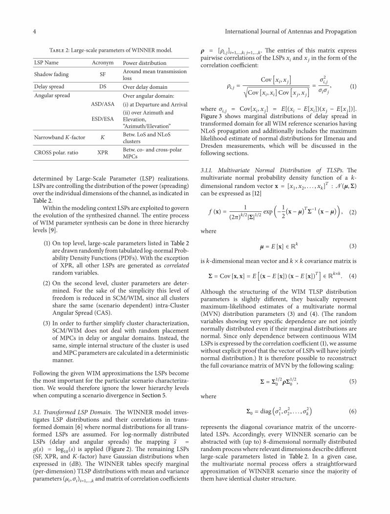
Table 2 Large-scale parameters of WINNER model
LSP Name Acronym Power distribution
Shadow fading SFAround mean transmissionloss
Delay spread DS Over delay domain
Angular spread Over angular domain
ASDASA (i) at Departure and Arrival
ESDESA(ii) over Azimuth andElevationldquoAzimuthElevationrdquo
Narrowband 119870-factor 119870 Betw LoS and NLoSclusters
CROSS polar ratio XPRBetw co- and cross-polarMPCs
determined by Large-Scale Parameter (LSP) realizationsLSPs are controlling the distribution of the power (spreading)over the individual dimensions of the channel as indicated inTable 2
Within the modeling context LSPs are exploited to governthe evolution of the synthesized channel The entire processof WIM parameter synthesis can be done in three hierarchylevels [9]
(1) On top level large-scale parameters listed in Table 2are drawn randomly from tabulated log-normal Prob-ability Density Functions (PDFs) With the exceptionof XPR all other LSPs are generated as correlatedrandom variables
(2) On the second level cluster parameters are deter-mined For the sake of the simplicity this level offreedom is reduced in SCMWIM since all clustersshare the same (scenario dependent) intra-ClusterAngular Spread (CAS)
(3) In order to further simplify cluster characterizationSCMWIM does not deal with random placementof MPCs in delay or angular domains Instead thesame simple internal structure of the cluster is usedand MPC parameters are calculated in a deterministicmanner
Following the given WIM approximations the LSPs becomethe most important for the particular scenario characteriza-tion We would therefore ignore the lower hierarchy levelswhen computing a scenario divergence in Section 5
31 Transformed LSP Domain The WINNER model inves-tigates LSP distributions and their correlations in trans-formed domain [6] where normal distributions for all trans-formed LSPs are assumed For log-normally distributedLSPs (delay and angular spreads) the mapping 119904 =119892(119904) = log10(119904) is applied (Figure 2) The remaining LSPs(SF XPR and 119870-factor) have Gaussian distributions whenexpressed in (dB) The WINNER tables specify marginal(per-dimension) TLSP distributions with mean and varianceparameters (120583119894 120590119894)119894=1119896 and matrix of correlation coefficients
120588 = [120588119894119895]119894=1119896 119895=1119896 The entries of this matrix expresspairwise correlations of the LSPs 119909119894 and 119909119895 in the form of thecorrelation coefficient
120588119894119895 = Cov [119909119894 119909119895]radicCov [119909119894 119909119894]Cov [119909119895 119909119895]
= 1205902119894119895120590119894120590119895 (1)
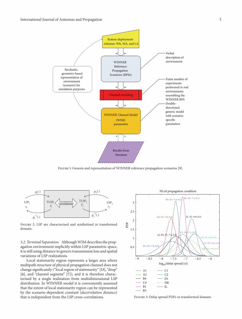
where 120590119894119895 = Cov[119909119894 119909119895] = 119864[(119909119894 minus 119864[119909119894])(119909119895 minus 119864[119909119895])]Figure 3 shows marginal distributions of delay spread intransformed domain for all WIM reference scenarios havingNLoS propagation and additionally includes the maximumlikelihood estimate of normal distributions for Ilmenau andDresden measurements which will be discussed in thefollowing sections
311 Multivariate Normal Distribution of TLSPs Themultivariate normal probability density function of a 119896-
dimensional random vector x = [1199091 1199092 119909119896]119879 N(120583Σ)can be expressed as [12]
119891 (x) = 1(2120587)1198962|Σ|12 exp(minus12(x minus 120583)
119879Σminus1 (x minus 120583)) (2)
where
120583 = 119864 [x] isin R119896 (3)
is 119896-dimensional mean vector and 119896 times 119896 covariance matrix is
Σ = Cov [x x] = 119864 [(x minus 119864 [x]) (x minus 119864 [x])119879] isin R119896times119896 (4)
Although the structuring of the WIM TLSP distributionparameters is slightly different they basically representmaximum-likelihood estimates of a multivariate normal(MVN) distribution parameters (3) and (4) (The randomvariables showing very specific dependence are not jointlynormally distributed even if their marginal distributions arenormal Since only dependence between continuous WIMLSPs is expressed by the correlation coefficient (1) we assumewithout explicit proof that the vector of LSPs will have jointlynormal distribution) It is therefore possible to reconstructthe full covariance matrix of MVN by the following scaling
Σ = Σ120 120588Σ120 (5)
where
Σ0 = diag (12059021 12059022 1205902119896) (6)
represents the diagonal covariance matrix of the uncorre-lated LSPs Accordingly every WINNER scenario can beabstracted with (up to) 8-dimensional normally distributedrandom process where relevant dimensions describe differentlarge-scale parameters listed in Table 2 In a given casethe multivariate normal process offers a straightforwardapproximation of WINNER scenario since the majority ofthem have identical cluster structure
International Journal of Antennas and Propagation 5
WINNERReference
PropagationScenarios (RPSs)
System-deployment schemes WA MA and LA
Verbaldescription ofenvironment
Channel sounding
Finite number of experimentsperformed in real environments resembling the WINNER RPS
WINNER Channel Model(WIM)
parameters
Double-directionalgeneric model with scenario-specificparameters
Stochastic
(scenario) for simulation purposes
Results from literature
representation ofenvironment
geometry-based
Figure 1 Genesis and representation of WINNER reference propagation scenarios [9]
correlations
Figure 2 LSP are characterized and synthetized in transformeddomain
32 Terminal Separation Although WIM describes the prop-agation environment implicitly within LSP parametric spaceit is still using distance to govern transmission loss and spatialvariations of LSP realizations
Local stationarity region represents a larger area wheremultipath structure of physical propagation channel does notchange significantly (ldquolocal region of stationarityrdquo [13] ldquodroprdquo[6] and ldquochannel segmentrdquo [7]) and it is therefore charac-terized by a single realization from multidimensional LSPdistribution In WINNER model it is conveniently assumedthat the extent of local stationarity region can be representedby the scenario-dependent constant (decorrelation distance)that is independent from the LSP cross-correlations
A1
A2
B4
C4
B1
B3
C1
C2
D1
DR
IL
minus9 minus85 minus8 minus75 minus7 minus65 minus6
05
1
15
2
25
3
NLoS propagation condition
log10(delay spread (s))
Figure 3 Delay spread PDFs in transformed domain
6 International Journal of Antennas and Propagation
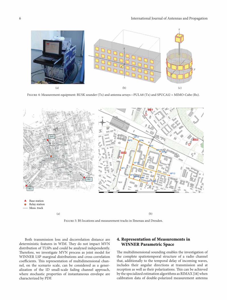
(a) (b) (c)
Figure 4 Measurement equipment RUSK sounder (Tx) and antenna arraysmdashPULA8 (Tx) and SPUCA12 + MIMO-Cube (Rx)
BS3
03
15
16
17
20
41a4140a
39
14 22
13
13a
13b
12c
25
2304
5a5b
05
24
28
10a10b
06
0807
11
9b
12a
12b4221
9a
40
01 BS1
02
BS2
Base stationRelay station
Meas track
(a) (b)
Figure 5 BS locations and measurement tracks in Ilmenau and Dresden
Both transmission loss and decorrelation distance aredeterministic features in WIM They do not impact MVNdistribution of TLSPs and could be analyzed independentlyTherefore we investigate MVN process as joint model forWINNER LSP marginal distributions and cross-correlationcoefficients This representation of multidimensional chan-nel on the scenario scale can be considered as a gener-alization of the 1D small-scale fading channel approachwhere stochastic properties of instantaneous envelope arecharacterized by PDF
4 Representation of Measurements inWINNER Parametric Space
The multidimensional sounding enables the investigation ofthe complete spatiotemporal structure of a radio channelthat additionally to the temporal delay of incoming wavesincludes their angular directions at transmission and atreception as well as their polarizations This can be achievedby the specialized estimation algorithms as RIMAX [14] whencalibration data of double-polarized measurement antenna
International Journal of Antennas and Propagation 7
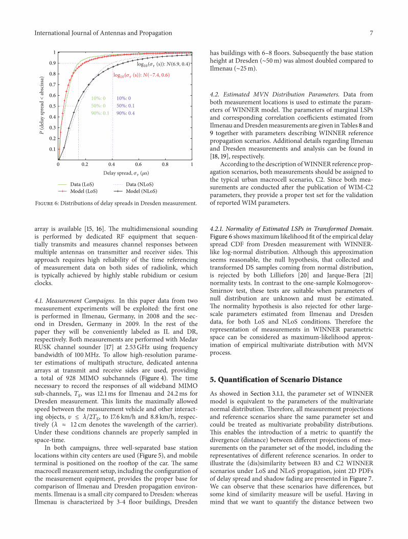
0 02 04 06 08 1
Data (LoS)
Model (LoS)
Data (NLoS)
Model (NLoS)
01
02
03
04
05
06
07
08
09
1
10 0
50 01
90 04
10 0
50 0
90 01
Figure 6 Distributions of delay spreads in Dresden measurement
array is available [15 16] The multidimensional soundingis performed by dedicated RF equipment that sequen-tially transmits and measures channel responses betweenmultiple antennas on transmitter and receiver sides Thisapproach requires high reliability of the time referencingof measurement data on both sides of radiolink whichis typically achieved by highly stable rubidium or cesiumclocks
41 Measurement Campaigns In this paper data from twomeasurement experiments will be exploited the first oneis performed in Ilmenau Germany in 2008 and the sec-ond in Dresden Germany in 2009 In the rest of thepaper they will be conveniently labeled as IL and DRrespectively Both measurements are performed with MedavRUSK channel sounder [17] at 253 GHz using frequencybandwidth of 100 MHz To allow high-resolution parame-ter estimations of multipath structure dedicated antennaarrays at transmit and receive sides are used providinga total of 928 MIMO subchannels (Figure 4) The timenecessary to record the responses of all wideband MIMOsub-channels 119879119878 was 121 ms for Ilmenau and 242 ms forDresden measurement This limits the maximally allowedspeed between the measurement vehicle and other interact-ing objects 119907 le 1205822119879119878 to 176 kmh and 88 kmh respec-tively (120582 asymp 12 cm denotes the wavelength of the carrier)Under these conditions channels are properly sampled inspace-time
In both campaigns three well-separated base stationlocations within city centers are used (Figure 5) and mobileterminal is positioned on the rooftop of the car The samemacrocell measurement setup including the configuration ofthe measurement equipment provides the proper base forcomparison of Ilmenau and Dresden propagation environ-ments Ilmenau is a small city compared to Dresden whereasIlmenau is characterized by 3-4 floor buildings Dresden
has buildings with 6ndash8 floors Subsequently the base stationheight at Dresden (sim50 m) was almost doubled compared toIlmenau (sim25 m)
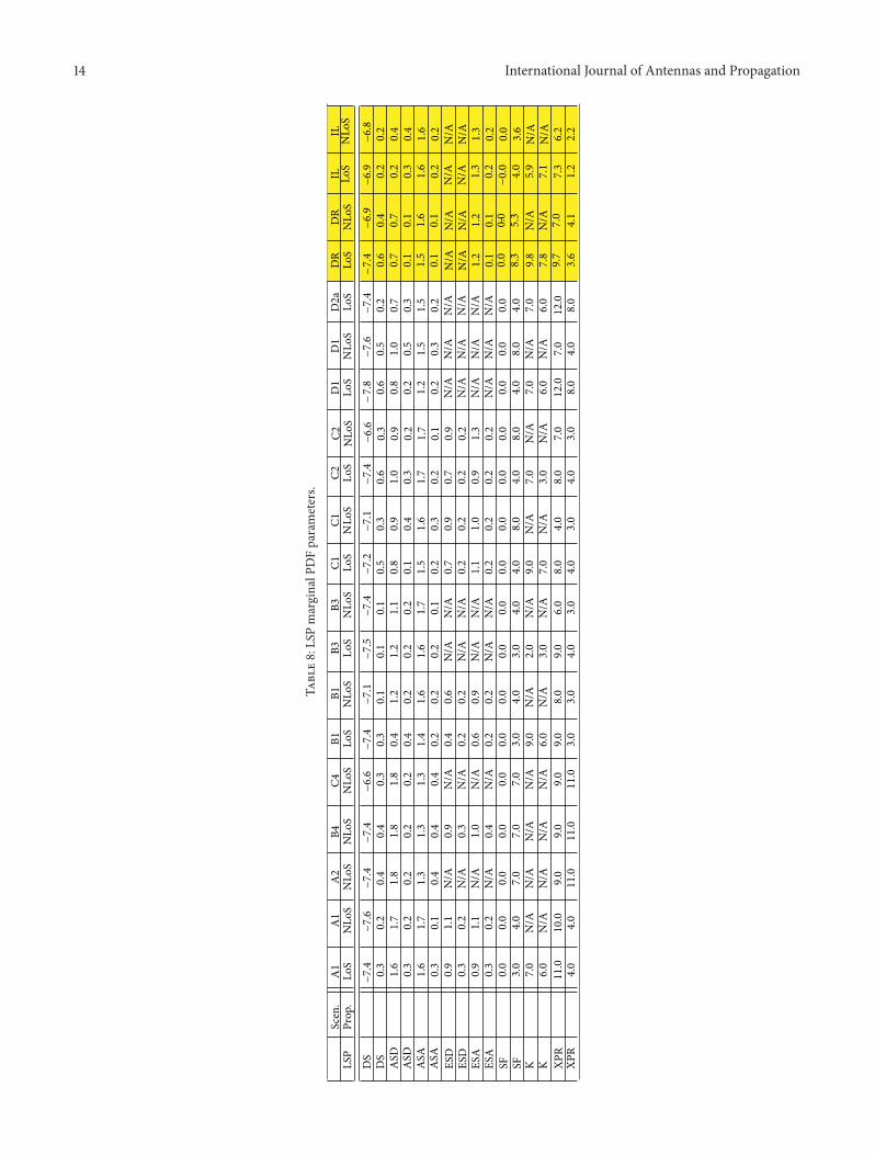
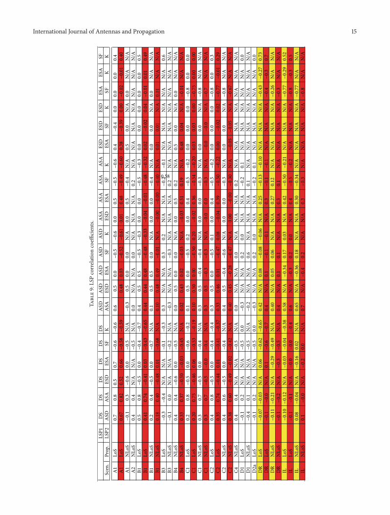
42 Estimated MVN Distribution Parameters Data fromboth measurement locations is used to estimate the param-eters of WINNER model The parameters of marginal LSPsand corresponding correlation coefficients estimated fromIlmenau and Dresden measurements are given in Tables 8 and9 together with parameters describing WINNER referencepropagation scenarios Additional details regarding Ilmenauand Dresden measurements and analysis can be found in[18 19] respectively
According to the description of WINNER reference prop-agation scenarios both measurements should be assigned tothe typical urban macrocell scenario C2 Since both mea-surements are conducted after the publication of WIM-C2parameters they provide a proper test set for the validationof reported WIM parameters
421 Normality of Estimated LSPs in Transformed DomainFigure 6 shows maximum likelihood fit of the empirical delayspread CDF from Dresden measurement with WINNER-like log-normal distribution Although this approximationseems reasonable the null hypothesis that collected andtransformed DS samples coming from normal distributionis rejected by both Lilliefors [20] and Jarque-Bera [21]normality tests In contrast to the one-sample Kolmogorov-Smirnov test these tests are suitable when parameters ofnull distribution are unknown and must be estimatedThe normality hypothesis is also rejected for other large-scale parameters estimated from Ilmenau and Dresdendata for both LoS and NLoS conditions Therefore therepresentation of measurements in WINNER parametricspace can be considered as maximum-likelihood approx-imation of empirical multivariate distribution with MVNprocess
5 Quantification of Scenario Distance
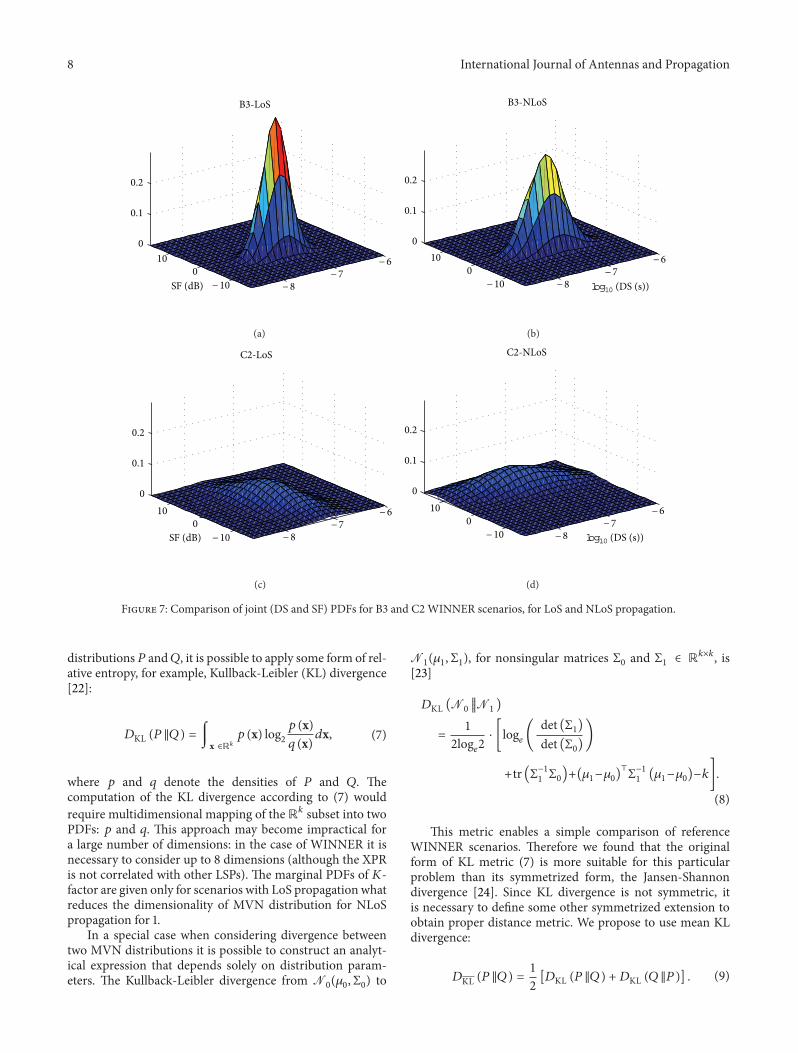
As showed in Section 311 the parameter set of WINNERmodel is equivalent to the parameters of the multivariatenormal distribution Therefore all measurement projectionsand reference scenarios share the same parameter set andcould be treated as multivariate probability distributionsThis enables the introduction of a metric to quantify thedivergence (distance) between different projections of mea-surements on the parameter set of the model including therepresentatives of different reference scenarios In order toillustrate the (dis)similarity between B3 and C2 WINNERscenarios under LoS and NLoS propagation joint 2D PDFsof delay spread and shadow fading are presented in Figure 7We can observe that these scenarios have differences butsome kind of similarity measure will be useful Having inmind that we want to quantify the distance between two
8 International Journal of Antennas and Propagation
0
10
0
B3-LoS
minus10 minus8minus7
minus6
02
01
SF (dB)
(a)
0
10
B3-NLoS
minus10 minus8minus7
minus60
02
01
log10 (DS (s))
(b)
C2-LoS
0
02
01
0
10
minus10 minus8minus7
minus6SF (dB)
(c)
C2-NLoS
0
02
01
minus8minus7
minus60
10
minus10 log10 (DS (s))
(d)
Figure 7 Comparison of joint (DS and SF) PDFs for B3 and C2 WINNER scenarios for LoS and NLoS propagation
distributions119875 and119876 it is possible to apply some form of rel-ative entropy for example Kullback-Leibler (KL) divergence[22]
119863KL (119875 119876) = intx isinR119896
119901 (x) log2119901 (x)119902 (x) 119889x (7)
where 119901 and 119902 denote the densities of 119875 and 119876 Thecomputation of the KL divergence according to (7) would
require multidimensional mapping of the R119896 subset into twoPDFs 119901 and 119902 This approach may become impractical fora large number of dimensions in the case of WINNER it isnecessary to consider up to 8 dimensions (although the XPRis not correlated with other LSPs) The marginal PDFs of 119870-factor are given only for scenarios with LoS propagation whatreduces the dimensionality of MVN distribution for NLoSpropagation for 1
In a special case when considering divergence betweentwo MVN distributions it is possible to construct an analyt-ical expression that depends solely on distribution param-eters The Kullback-Leibler divergence from N0(1205830 Σ0) to
N1(1205831 Σ1) for nonsingular matrices Σ0 and Σ1 isin R119896times119896 is[23]
119863KL (N0 1003817100381710038171003817N1 )= 12log1198902 sdot [log119890 ( det (Σ1)
det (Σ0))+tr (Σminus11 Σ0)+(1205831minus1205830)⊤Σminus11 (1205831minus1205830)minus119896]
(8)
This metric enables a simple comparison of referenceWINNER scenarios Therefore we found that the originalform of KL metric (7) is more suitable for this particularproblem than its symmetrized form the Jansen-Shannondivergence [24] Since KL divergence is not symmetric itis necessary to define some other symmetrized extension toobtain proper distance metric We propose to use mean KLdivergence
119863KL (119875 119876) = 12 [119863KL (119875 119876) + 119863KL (119876 119875)] (9)
International Journal of Antennas and Propagation 9
51 Negative Definite Covariance Matrices In some casesnegative or complex values are obtained for KL divergenceindicating that the matrix of correlation coefficients (120588) isnot positive semidefinite that is 120588 lt 0 The problem ismanifesting only for scenarios with resolved elevation angles(Table 3) where the dimensionality of the MVN distributionis increased from 6 (LoS)5 (NLoS) to 76 or 87 The problemis however not related to the number of dimensions orelevation parameters themselves since simple removal ofelevation dimension(s) does not resolve it This means thatcorrelation coefficients between WINNER LSPs analyzedjointly do not form a proper correlation matrix (CM)mdashnoteven without elevations
It is observed that the number of decimal places used forrepresentation of CM elements cannot be arbitrarily reducedsince the resulting matrix may become negative definiteSince individual coefficients in WINNER parameter tablesare expressed using only one decimal place it is possiblethat this lack of precision causes negative definite CM forscenarios with an increased number of dimensions
In order to enable the comparison of problematic scenar-ios their correlation coefficients have to be slightly modifiedto form positive definite CM The ldquorealrdquo correlation matrixis computed using alternate projections method (APM) [25
26] For a given symmetric matrix120588 isin R119896119909119896 this method findsthe nearest correlation matrix that is (semi) definite andhas units along the main diagonal The solution is found inthe intersection of the following sets of symmetric matrices
119878 = 119884 = 119884119879 isin R119896119909119896 | 119884 ge 0 and119880 = 119884 = 119884119879 isin R119896119909119896 | 119910119894119894 =1 119894 = 1 119896 The iterative procedure in 119899th step appliesupdated Dykstrarsquos correctionΔ119878119899minus1 and subsequently projectsintermediate result to both matrix sets using projections 119875119878and 119875119880
ΔS0 = 0 Y0 = 120588 119899 = 0do
119899 = 119899 + 1R119899 = Y119899minus1 minus ΔS119899minus1X119899 = 119875119878 (R119899)ΔS119899minus1 = X119899 minus R119899
Y119899 = 119875119880 (X119899)while
1003817100381710038171003817Y119899 minus Y119899minus11003817100381710038171003817119865 lt 119905119900119897
(10)
The projection 119875119878 replaces all negative eigenvalues of thematrix with a small positive constant 120598 and 119875119880 forcesones along the main diagonal The procedure stops whenFrobenius distance sdot 119865 between 119884119899 projections from twoconsecutive iterations drops below a predefined tolerance 119905119900119897Note however that the small tolerance parameter does notinsure that Frobenius distance (FD) from the original matrixis equally small
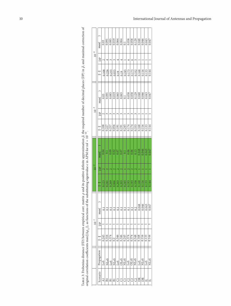
The positive definite approximation obtained by APMwill depend on the selected parameters 120598 and 119905119900119897 [27] for119905119900119897 = 10minus10 the effect of eigenvalue 120598 on Frobenius distance
FD = 120588 minus 119865 is illustrated in Table 3 The results show thatFD decreases when a smaller value of 120598 is used to substituteoriginally negative eigenvalues However the selection ofsmall 120598 will proportionally increase the eigenvalues and
coefficients of the inverse correlation matrix minus1 This willconsequently increase the KL divergence (7) to all otherscenarios As a compromise the new WINNER correlationcoefficients corresponding to positive definite matrix are
recomputed for 120598 = 10minus2 and 119905119900119897 = 10minus10 and given in Table 9The maximal absolute modification of original correlationcoefficients per scenario max|Δ120588119894119895| whereΔ120588119894119895 = 120588119894119895minus120588119894119895is given in Table 3 The highest absolute correction Δ120588 = 013is applied to C2-NLoS scenario
The minimum number of decimal places required to keep positive definite is determined for different values of 120598 andlisted in Table 3 The results show that smaller Frobeniusdistance requires higher precision for saving coefficients
For 120598 = 10minus2 two decimal places are sufficient to expresscorrelation coefficients for all scenarios (Table 9)
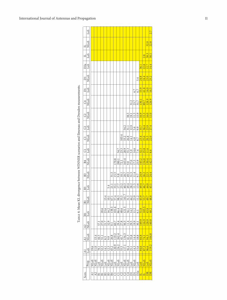
52 Mean KL Divergence In order to enable comparisonsbetween LoS and NLoS scenarios where 119870-factor is missingunder NLoS as well as other scenarios where certain param-eters (dimensions) are missing the reduction of dimension-ality was necessary only those dimensions existing in bothscenarios are used to calculate the mean KL divergenceThis means that scenarios with lower number of resolveddimensions could exhibit more similarity as a consequenceof incomplete representation A fair comparison would bepossible only if all scenarios have the same number ofdimensions The respective mean KL divergences betweenall WINNER scenarios including Ilmenau and Dresdenmeasurements are given in Table 4 (for WINNER scenariosthat give two sets of LoS parameters mean KL distances arecomputed for LoS parameters before breakpoint distance oftransmission loss)
In order to simplify the analysis of obtained results foreach (scenario propagation) combination the closest matchis found and listed in Table 5 Divergences within the sameWINNER scenario group or having same propagation con-ditions are not minimum as may have been expected Table 5shows that only 5 among 16 WINNER scenarios have theclosest match within the same WINNER group (A B C andD) This comes as consequence of subjective classification ofsimilar environments without previously introduced metricThe minimum distances from Table 5 119863KL = 01 confirmsome expectations B4-NLoS (outdoor-to-indoor) is closestto A2-NLoS (indoor-to-outdoor) because these are reciprocalscenarios Also microcell and macrocell versions of outdoor-to-indoor (B4 and C4) are the closest although not belongingto the same group Mean KL divergences from Table 5 suggestthat there is a better way to group available scenarios
The average distances between all scenarios from oneWINNER group to all scenarios in the other groups are givenin Table 6 If all groups gather the most similar scenariosan average distance between any two groups will be higherthan the average distance within a single group From Table 6we can see that this applies to groups A and D which
10 International Journal of Antennas and Propagation
Ta
ble
3F
rob
eniu
sd
ista
nce
(FD
)b
etw
een
emp
iric
alco
rr
mat
rix120588an
dit
sp
osi
tive
defi
nit
eap
pro
xim
atio
n120588t
he
req
uir
edn
um
ber
of
dec
imal
pla
ces
(DP
)in120588a
nd
max
imal
corr
ecti
on
of
ori
gin
alco
rrel
atio
nco
effici
ents
max|Δ120588119894119895|a
sfu
nct
ion
so
fth
esu
bst
itu
tin
gei
gen
valu
e120598in
AP
Mfo
r119905119900119897
=10minus10
A1
Lo
S0245
101
0123
2004
0108
20
03
0108
20
03
B4
NL
oS
0316
101
0241
201
0227
30
091
0226
40
091
B1
Lo
S0374
101
0269
2009
0257
30
085
0255
30
085
B1
NL
oS
02
101
0 066
2002
0056
30
019
0055
30
019
C1
Lo
S0346
101
0203
2007
0191
30
065
019
40
064
C1
OL
oS
0346
101
0203
2007
0191
30
065
019
40
064
C1
NL
oS
0245
101
0245
101
0245
101
0245
101
C2
Lo
S0374
101
0193
2006
0174
30
058
0173
60
058
C2
OL
oS
0374
101
0193
2006
0174
30
058
0173
60
058
C2
NL
oS
0548
102
0338
2013
0333
30
129
0332
50
129
DR
Lo
S0168
10048
0168
10048
0168
10
048
0168
10
048
DR
NL
oS
0116
10046
0116
10046
0116
10
046
0116
10
046
ILL
oS
0133
10043
0133
10043
0133
10
043
0133
10
043
ILN
Lo
S0144
10047
0144
10
047
0144
10 047
0144
10047
Sce
nar
io
10minus1
10minus2
10minus3
10minus6
Pro
pag
atio
nD
PD
PD
PD
Pm
ax(
)m
ax(
)m
ax(
)m
ax(
)sdot
sdotsdot
sdot
International Journal of Antennas and Propagation 11
Ta
ble
4M
ean
KL
div
erge
nce
bet
wee
nW
INN
ER
scen
ario
san
dIl
men
auan
dD
resd
enm
easu
rem
ents
Sce
n
A1
A2
B1
B1
B3
B3
B4
C1
C1
C2
C2
C4
D1
D1
D2a
IL IL DR
DR
Pro
p
NL
oS
NL
oS
Lo
SN
Lo
SL
oS
NL
oS
NL
oS
Lo
SN
Lo
SL
oS
NL
oS
NL
oS
Lo
SN
Lo
SL
oS
Lo
SN
Lo
SL
oS
NL
oS
A1
Lo
S 196
110
781
523
141
123
452
120
922
42
555
117
136
425
114
315
684
687
396
611
92
A1
NL
oS
154
445
511
83
99
268
119
226
24
417
134
341
335
814
418
864
874
194
310
48
A2
NL
oS
571
270
217
329
01
607
294
278
503
114
295
199
301
149
911
69
128
914
08
B1
Lo
S 206
236
162
138
510
16
864
486
121
556
114
211
26
151
810
55
438
482
B1
NL
oS
154
101
671
574
983
555
141
731
544
223
911
245
953
749
748
8
B3
Lo
S 54
211
331
177
232
403
494
282
115
136
494
467
440
451
B3
NL
oS
315
155
98
101
207
495
315
114
97
249
262
225
244
B4
NL
oS
170
828
01
721
163
49
827
017
525
914
52
154
013
04
142
3
C1
Lo
S
547
235
289
553
59
146
74
325
258
116
86
C1
NL
oS
103
433
226
814
14
88
723
425
620
322
0
C2
Lo
S
542
311
129
56
99
357
364
239
274
C2
NL
oS
385
191
115
159
169
153
160
110
C4
NL
oS
312
237
317
130
189
712
89
126
9
D1
Lo
S
67
67
559
418
140
165
D1
NL
oS
54
248
244
230
252
D2a
Lo
S
361
228
127
144
IL Lo
S
28
383
301
IL NL
oS
320
228
Lo
S
27
12 International Journal of Antennas and Propagation
minus15
minus10
minus5
0
5
10
15
SF
(d
B)
1 11 12 13 14 15
PDFmax = 016
log10 (ESA (deg))
(a)
PDFmax = 44
15 16 17 18 19 2
minus72
minus7
minus68
minus66
minus64
minus62
minus6
log10(
DS
(s))
log10 (ASA (deg))
(b)
ρc = minus 04
PDFmax = 0099
minus15
minus10
minus5
0
5
10
15
SF
(d
B)
06 08 1 12
log10 (ASD (deg))
(c)
PDFmax = 5615
16
17
18
19
2
log10(
AS
A (
deg
))
06 08 1 12
log10 (ASD (deg))
(d)
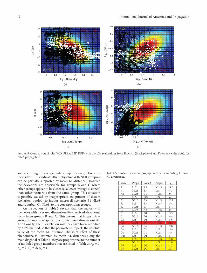
Figure 8 Comparison of joint WINNER C2 2D PDFs with the LSP realizations from Ilmenau (black pluses) and Dresden (white dots) forNLoS propagation
are according to average intergroup distance closest tothemselves This indicates that subjective WINNER groupingcan be partially supported by mean KL distance Howeverthe deviations are observable for groups B and C whereother groups appear to be closer (at a lower average distance)than other scenarios from the same group This situationis possibly caused by inappropriate assignment of distantscenarios outdoor-to-indoor microcell scenario B4-NLoSand suburban C1-NLoS to the corresponding groups
An inspection of Table 3 reveals that the majority ofscenarios with increased dimensionality (resolved elevations)come from groups B and C This means that larger intra-group distance may appear due to increased dimensionalityAdditionally their correlation matrices have been modifiedby APM method so that the parameter 120598 impacts the absolutevalue of the mean KL distance The joint effect of thesephenomena is illustrated by mean KL distances along themain diagonal of Table 6 they are proportional to the numberof modified group members that are listed in Table 3 D = 0A = 1 B = 3 C = 6
Table 5 Closest (scenario propagation) pairs according to meanKL divergence
Scen1 Prop1 Scen2 Prop2A1 LoS A2 NLoS 110A1 NLoS B3 LoS 83A2 NLoS B4 NLoS 01B1 LoS D2a LoS 61B1 NLoS B3 NLoS 101B3 LoS B3 NLoS 54B3 NLoS B3 LoS 54B4 NLoS A2 NLoS 01C1 LoS D1 LoS 59C1 NLoS D1 NLoS 48C2 LoS D1 NLoS 56C2 NLoS DR NLoS 110C4 NLoS B4 NLoS 98D1 LoS C1 LoS 59D1 NLoS C1 NLoS 48D2a LoS D1 NLoS 54IL LoS IL NLoS 28IL NLoS IL LoS 28DR LoS DR NLoS 27DR NLoS DR LoS 27
KL
International Journal of Antennas and Propagation 13
Table 6 Average distance between WINNER scenario groups A BC and D
A B C D
A 153
B 321 350
C 888 706 450
D 226 191 145 63
Table 7 Average distance between WINNER LoS and NLoSpropagation conditions
LoS NLoS
LoS 318
NLoS 421 509
For 6 out of 16 (scenario propagation) pairs the bestmatch has the opposite propagation condition (LoS insteadof NLoS and vice versa) indicating that WINNER LoS andNLoS parameters do not form disjunctive sets (Table 5)Calculation of the mean distance between all LoS andNLoS scenarios in Table 7 shows that lower average distancecan be expected between scenarios having LoS propagationcondition (they are more similar than different scenarios withNLoS propagation)
6 Classification of Measurements
The same criterion KL divergence can be applied to classifymeasurements as well For this purpose even empiricaldistributions of LSPs can be used since KL metric (7) supportsthat However the extraction of the corresponding WINNERparameters simplifies the comparison since analytical expres-sion (8) can be applied Therefore we use the latter approachto compare Ilmenau and Dresden measurements with otherWINNER scenarios
Since both measurements have been performed in urbanenvironments with macrocell setup (antennas were elevatedabove rooftops) it is expected that the closest scenario willbe WINNER C2 which represents typical urban macro-cells These expectations are met for Ilmenau measurementswhere WINNER C2-NLoS is the closest scenario for bothLoS and NLoS conditions with minimal distances 119863KL =169 and 119863KL = 153 (Table 4) In the case of Dresdenmeasurements minimal mean KL divergences (86 and 116)indicate that the closest WIM scenario is C1-LoS for bothLoS and NLoS propagation conditions This resemblance ofDresden measurements to suburban propagation (WINNERC1) may come from dominant height of BS positions withrespect to environment
Figure 8 shows the 2D PDFs of the reference WINNERC2-NLoS scenario together with joint LSP realizations fromIlmenau and Dresden measurements For the NLoS propaga-tion condition Ilmenau and Dresden measurements are quiteclose to C2 C2-NLoS is the best match for Ilmenau-NLoS(119863KL = 163) and the second best match for Dresden-NLoSdata (119863KL = 11) Additionally among all results presented in
Table 4 the closest match of WIM C2-NLoS is just Dresden-NLoS (row showed in red)
For LoS conditions distances from WINNER C2 andIlmenau and Dresden measurements are larger (357 and239) which classifies Ilmenau-LoS to C2-NLoS (119863KL = 169)and Dresden-LoS into C1-LoS (119863KL = 116) Table 5 showsthe increased similarity between LoS and NLoS propagationconditions in Ilmenau and Dresden measurements Thisoccurs also for WINNER B3 while other WINNER scenariosdo not show this property One possible interpretation comesfrom the data segmentation into LoS and NLoS classes theactual propagation conditions for the LoS or NLoS-labeleddata may actually correspond to for example obstructedline of sight (OLoS) The previous analysis demonstratesthat mean KL divergence additionally to the comparisonof different measurements enables the quantification ofcomplex relations between different data segments of thesame measurement as long as they use the same LSP spacerepresentation
The mean KL distances between Ilmenau and Dresdenmeasurements (383-LoS and 228-NLoS) are higher thancorresponding distances from these measurements to the ref-erence WINNER-C2 scenario This confirms that WINNERC2 parameters provide appropriate representation for a wideclass of urban macro-cell environments
7 Conclusions
The paper presents the scenario concept of WINNER andproposes its abstraction to a multivariate normal distributionof large-scale parameters Disregarding transmission lossand decorrelation distance removes the spatial extent fromscenario definitions
The generic property of the model is exploited to comparethe large-scale parameters that describe different scenariosFor this purpose a symmetrized extension of the Kullback-Leibler divergence is proposed This enables the comparisonof parameters between reference scenarios and measure-ments as well as a direct comparison of empirical LSPdistributions (measured or synthesized by channel model)The given approach can be also applied to other genericstochastic models if appropriate metrics are chosen thatreflect modelsrsquo specifics
The presented results indicate that according to the meanKullback-Leibler divergence WINNER scenario groups orpropagation classes do not ensure the minimum separa-tion within the groupclass It appears that other criteriafor example coverage range were more significant forthe WINNER taxonomy Judged from the mean Kullback-Leibler divergence large similarity exists between the indoor-to-outdoor and outdoor-to-indoor scenarios (A2 B4 andC4) between macro-cell configurations for suburban urbanand rural scenarios (C1 C2 and D1) and between theindoorhotspotmicrocellular scenarios (A1 B3 and B1)
It is demonstrated that the results of measurementscould be associated with the closest WINNER scenarioAs expected typical urban macro-cell scenario C2 was theone closest to the Ilmenau measurements For the Dresden
14 International Journal of Antennas and Propagation
Ta
ble
8L
SPm
argi
nal
PD
Fp
aram
eter
s
Sce
n
A1
A1
A2
B4
C4
B1
B1
B3
B3
C1
C1
C2
C2
D1
D1
D2a
DR
DR
ILIL
LSP
Pro
p
Lo
SN
Lo
SN
Lo
SN
Lo
SN
Lo
SL
oS
NL
oS
Lo
SN
Lo
SL
oS
NL
oS
Lo
SN
Lo
SL
oS
NL
oS
Lo
SL
oS
NL
oS
Lo
SN
Lo
S
DS
minus74
minus76minus7
4minus7
4minus6
6minus7
4minus7
1minus7
5minus7
4minus7
2minus7
1minus7
4minus6
6minus7
8minus7
6minus7
4minus7
4minus6
9minus6
9minus6
8D
S0
30
20
40
40
30
30
10
10
10
50
30
60
30
60
50
20
60
40
20
2A
SD1
61
71
81
81
80
41
21
21
10
80
91
00
90
81
00
70
70
70
20
4A
SD0
30
20
20
20
20
40
20
20
20
10
40
30
20
20
50
30
10
10
30
4A
SA1
61
71
31
31
31
41
61
61
71
51
61
71
71
21
51
51
51
61
61
6A
SA0
30
10
40
40
40
20
20
20
10
20
30
20
10
20
30
20
10
10
20
2E
SD0
91
1N
A0
9N
A0
40
6N
AN
A0
70
90
70
9N
AN
AN
AN
AN
AN
AN
AE
SD0
30
2N
A0
3N
A0
20
2N
AN
A0
20
20
20
2N
AN
AN
AN
AN
AN
AN
AE
SA0
91
1N
A1
0N
A0
60
9N
AN
A1
11
00
91
3N
AN
AN
A1
21
21
31
3E
SA0
30
2N
A0
4N
A0
20
2N
AN
A0
20
20
20
2N
AN
AN
A0
10
10
20
2SF
00
00
00
00
00
00
0 0
00
00
00
00
00
00
00
00
00
00minus00
minus 00
00
SF3
04
07
07
07
03
04
03
04
04
08
04
08
04
08
04
08
35
34
03
6K
70
NA
NA
NA
NA
90
NA
20
NA
90
NA
7 0
NA
70
NA
70
98
NA
59
NA
K6
0N
AN
AN
AN
A6
0N
A3
0N
A7
0N
A3
0N
A6
0N
A6
07
8N
A7
1N
A
XP
R11
010
09
09
09
09
08
09
06
08
04
08
07
012
07
012
09
77
07
36
2X
PR
40
40
110
110
110
30
30
40
30
40
30
40
30
80
40
80
36
41
12
22
International Journal of Antennas and Propagation 15
Ta
ble
9L
SPco
rrel
atio
nco
effici
ents
LS
P1
DS
DS
DS
DS
DS
DS
AS
DA
SDA
SD
ASD
AS
DA
SAA
SA
ASA
AS
AE
SDE
SD
ESD
ESA
ESA
SFS
cen
P
rop
L
SP2
ASD
AS
AE
SDE
SASF
KA
SAE
SD
ESA
SFK
ESD
ESA
SFK
ESA
SFK
SF
KK
A1
Lo
S0
70
80
50
7minus0
6minus0
60
60
50
0minus0
5minus0
60
00
5minus0
5minus0
60
4minus0
40
00
00
00
4A
1L
oS
067
082
052
066minus0
58minus0
59
058
048
003
minus0
52minus0
61
001
048minus0
49minus0
60
038minus0
39
000minus0
02minus0
01
040
A1
NL
oS
minus01
03minus0
60
0minus0
5N
Aminus0
30
50
00
0N
A0
00
5minus0
4N
A0
50
0N
A0
0N
AN
AA
2N
Lo
S0
40
4N
AN
Aminus0
5N
A0
0N
AN
A0
0N
AN
AN
A0
2N
AN
AN
AN
AN
AN
AN
AB
1L
oS
05
08minus0
50
0minus0
4minus0
70
40
50
5minus0
5minus0
30
00
0minus0
5minus0
30
00
00
00
00
00
5B
1L
oS
041
074minus0
41
003minus0
43minus0
65
044
044
048minus0
48minus0
33minus0
04minus0
01minus0
48minus0
32
002minus0
02
004minus0
01
001
049
B1
NL
oS
02
04minus0
50
0minus0
7N
A0
10
50
50
0N
A0
00
0minus0
4N
A0
00
0N
A0
0N
AN
AB
1N
Lo
S0
180
40minus0
48
001minus0
68
NA
010
048
049minus0
01
NAminus0
00minus0
00minus0
40
NA
001
001
NA
001
NA
NA
B3
Lo
Sminus0
3minus0
4N
AN
Aminus0
1minus0
30
3N
AN
A0
30
2N
AN
Aminus0
2minus0
1N
AN
AN
AN
AN
A0
6B
3N
Lo
Sminus0
10
0N
AN
Aminus0
2N
Aminus0
3N
AN
Aminus0
3N
AN
AN
A0
2N
AN
AN
AN
AN
AN
AN
AB
4N
Lo
S0
40
4minus0
60
0minus0
5N
A0
00
50
00
0N
A0
00
50
2N
A0
50
0N
A0
0N
AN
AB
4N
Lo
S0
330
37minus0
50minus0
03minus0
45
NA
002
043
002minus0
03
NAminus0
03
051
019
NA
048
004
NAminus0
01
NA
NA
C1
Lo
S0
20
8minus0
50
0minus0
6minus0
20
10
50
0minus0
50
20
00
4minus0
5minus0
20
00
00
0minus0
80
00
0C
1L
oS
020
075minus0
46
006minus0
53minus0
19
010
050
0 00minus0
50
020minus0
02
036minus0
54minus0
20
003
003
000minus0
75
000
000
C1
NL
oS
03
07minus0
50
0minus0
4N
A0
30
5minus0
4minus0
4N
A0
00
0minus0
3N
A0
00
0N
Aminus0
8N
AN
AC
1N
Lo
S0
30
7minus0
5minus0
0minus0
4N
A0
30
5minus0
3minus0
3N
Aminus0
00
0minus0
3N
Aminus0
0minus0
0N
Aminus0
7N
AN
AC
2L
oS
04
08minus0
50
0minus0
4minus0
40
30
50
0minus0
50
10
00
4minus0
5minus0
20
00
00
0minus0
80
00
3C
2L
oS
035
074minus0
44
001minus0
41minus0
37
033
046
001minus0
47
008minus0
04
039minus0
50
minus0
220
00minus0
02
002minus0
77minus0
01
029
C2
NL
oS
04
06minus0
50
0minus0
4N
A0
40
5minus0
4minus0
6N
A0
00
0minus0
3N
A0
00
0N
Aminus0
8N
AN
AC
2N
Lo
S0
380
60minus0
49minus0
02minus0
42
NA
040
045minus0
28minus0
47
NA
000minus0
00minus0
30
NAminus0
05minus0
05
NAminus0
67
NA
NA
C4
NL
oS
04
04
NA
NAminus0
5N
A0
0N
AN
A0
0N
AN
AN
A0
2N
AN
AN
AN
AN
AN
AN
AD
1L
oS
minus01
02
NA
NAminus0
50
0minus0
3N
AN
A0
20
0N
AN
Aminus0
20
1N
AN
AN
AN
AN
A0
0D
1N
Lo
Sminus0
40
1N
AN
Aminus0
5N
Aminus0
2N
AN
A0
6N
AN
AN
A0
1N
AN
AN
AN
AN
AN
AN
AD
2aL
oS
minus01
02
NA
NAminus0
50
0minus0
3N
AN
A0
20
0N
AN
Aminus0
20
1N
AN
AN
AN
AN
A0
0D
RL
oS
minus00
7minus0
03
NA
006minus0
62minus0
65
042
NA
008minus0
08minus0
06
NA
025minus0
13minus0
10
NA
NA
NAminus0
43minus0
27
073
DR
Lo
Sminus0
1minus0
0N
A0
1minus0
6minus0
70
4N
A0
1minus0
1minus0
1N
A0
3minus0
1minus
01
NA
NA
NAminus0
4minus0
30
7D
RN
Lo
Sminus0
11minus0
21
NAminus0
29minus0
49
NA
040
NA
005
006
NA
NA
027
012
NA
NA
NA
NAminus0
26
NA
NA
DR
NL
oS
minus01minus0
2N
Aminus0
3minus0
5N
A0
4N
A0
10
1N
AN
A0
30
1N
AN
AN
AN
Aminus0
3N
AN
AIL
Lo
Sminus0
10minus0
12
NAminus0
03minus0
04minus0
38
058
NAminus0
34
017
003
NA
042minus0
50minus0
21
NA
NA
NAminus0
77minus0
29
052
ILL
oS
minus01minus0
1N
Aminus0
0minus0
0minus0
40
6N
Aminus0
30
20
0N
A0
4minus0
5minus0
2N
AN
AN
Aminus0
8minus0
30
5IL
NL
oS
008minus0
04
NAminus0
16
002
NA
065
NAminus0
36
018
NA
NA
030minus0
34
NA
NA
NA
NAminus0
77
NA
NA
ILN
Lo
S0
1minus0
0N
Aminus0
20
0N
A0
7N
Aminus0
40
2N
AN
A0
3minus0
3N
AN
AN
AN
Aminus0
8N
AN
A
16 International Journal of Antennas and Propagation
measurements suburban LSP distributions of C1 were closestThis measurement however appears to be at minimumdistance from C2-NLoS indicating a validity of assumedmacro-cell measurement setup The proper choice of WIN-NER C2 parameters for representation of the whole class ofurban macrocells is confirmed by the Ilmenau and Dresdenmeasurements these measurements are closer to the C2reference than to each other
For those scenariosmeasurements where the correlationcoefficients form a negative definite symmetric matrix thealternating projection method is exploited to determinethe closest correlation matrix Therefore the paper alsointroduces the modified WINNER scenario parameters thatenable a quantification of scenario divergence
Appendix
Parameters of WINNER Channel ModelDescribing MVN Distributions
In order to ensure the traceability of the presented diver-gences the relevant subset of WINNER parameters is givenin Tables 8 and 9 They also include the MVN distributionparameters estimated from Ilmenau and Dresden measure-ments Additionally Table 9 contains the modified corre-lation coefficients 120588 that form positive definite correlationmatrices They are used for scenario representation insteadof original coefficients
Acknowledgment
The authors would like to acknowledge the contributions oftheir colleagues from EASY-C project during the conductionand analysis of measurements especially to Carsten JanduraActix GmbH
References
[1] A F Molisch H Asplund R Heddergott M Steinbauer andT Zwick ldquoThe COST259 directional channel model-part Ioverview and methodologyrdquo IEEE Transactions on WirelessCommunications vol 5 no 12 pp 3421ndash3433 2006
[2] ldquoDigital land mobile radio communicationsrdquo Tech RepCOST207 1989
[3] L Correia Ed Wireless Flexible Personalised CommunicationsCOST 259 European Co-Operation in Mobile Radio ResearchWiley 2001
[4] L Correia ldquoMobile broadband multimedia networksmdashtechniques models and tools for 4Grdquo Final Report COST 273Elsevier Oxford UK 2006
[5] R Verdone and A Zanella PervasiveMobile and AmbientWire-less Communications Signals and Communication TechnologySpringer London UK 2012
[6] 3GPP TR25996 V900 Spatial channel model for MIMO sim-ulationsThird Generation Partnership Project (3GPP) TechRep December 2009 httpwww3gpporg
[7] P Kyosti J Meinila L Hentila et al ldquoIST-4-027756 WINNERII Deliverable 112 v12 WINNER II Channel Modelsrdquo TechRep IST-WINNERII 2007
[8] Guidelines for evaluation of radio interface technologies forIMTAdvanced Report ITU-R M2135-1 International Telecom-munication Union Radiocommunication Sector (ITU-R)2009 httpwwwituintpubR-REP-M2135-1-
[9] M Narandzic C Schneider and R S Thoma ldquoWINNER wide-band MIMO system-level channel model comparison withother reference modelsrdquo in Proceedings of the InternationalesWissenschartliches Kolloquium (IWK rsquo09) vol 54 IlmenauGermany 2009
[10] WINNER (Wireless world INitiative NEw Radio) httpprojectsceltic-initiativeorgwinner+
[11] M Steinbauer A F Molisch and E Bonek ldquoThe double-directional radio channelrdquo IEEE Antennas and PropagationMagazine vol 43 no 4 pp 51ndash63 2001
[12] ldquoMultivariate normal distributionrdquo httpenwikipediaorgwikiMultivariate normal distribution
[13] A Gehring M Steinbauer I Gaspard and M Grigat ldquoEmpiri-cal channel stationarity in urban environmentsrdquo in Proceedingsof the European Personal Mobile Communications Conference(EPMCC rsquo01) Vienna Austria February 2001
[14] R Thoma M Landmann and A Richter ldquoRIMAXmdasha maxi-mum likelihood framework for parameter estimation in multi-dimensional channel soundingrdquo in Proceedings of the Interna-tional Symposium on Antennas and Propagation Sendai JapanAugust 2004
[15] M Landman M Narandzic and R S Thoma ldquoLimits of experi-mental channel characterization related to antenna calibrationrdquoin Proceedings of the 29th General Assembly of the InternationalUnion of Radio Science (URSI rsquo08) Chicago Ill USA August2008
[16] M Landmann M Kaske and R S Thoma ldquoImpact ofincomplete and inaccurate data models on high resolutionparameter estimation in multidimensional channel soundingrdquoIEEE Transactions on Antennas and Propagation vol 60 no 2pp 557ndash573 2012
[17] Rusk channel sounder httpwwwchannelsounderde
[18] C Schneider M Narandzic M Kaske G Sommerkorn and RS Thoma ldquoLarge Scale parameter for the WINNER II channelmodel at 2 53 GHz in urban macro cellrdquo in Proceedings of theIEEE 71st Vehicular Technology Conference (VTC rsquo10) TaipeiTaiwan May 2010
[19] M Narandzic C Schneider M Kaske S Jackel G Som-merkorn and R S Thoma ldquoLarge-scale parameters of wide-band MIMO channel in urban multi-cell scenariordquo in Pro-ceedings of the 5th European Conference on Antennas andPropagation (EUCAP rsquo11) pp 3759ndash3763 Rome Italy April 2011
[20] H W Lilliefors ldquoOn the Kolmogorov-Smirnov test for normal-ity with mean and variance unknownrdquo Journal of the AmericanStatistical Association vol 62 no 318 pp 399ndash402 1967
[21] C M Jarque and A K Bera ldquoA test for normality of observa-tions and regression residualsrdquo International Statistical Reviewvol 55 no 2 pp 163ndash172 1987
[22] S Kullback and R A Leibler ldquoOn information and sufficiencyrdquoThe Annals of Mathematical Statistics vol 22 no 1 pp 79ndash861951
[23] W D Penny and S J Roberts ldquoVariational bayes for generalisedautoregressive modelsrdquo Tech Rep PARG-00-12 Department ofEngineering Science Oxford University 2000
[24] B Fuglede and F Topsoslashe ldquoJensen-Shannon Divergence andHilbert space embeddingrdquo httpwwwmathkudksimtopsoeISIT2004JSDpdf
International Journal of Antennas and Propagation 17
[25] J P Boyle and R L Dykstra ldquoA method for finding projectionsonto the intersection of convex sets in Hilbert spacesrdquo Advancesin Order Restricted Inference vol 37 pp 28ndash47 1986
[26] N J Higham ldquoComputing the nearest correlation matrixmdashaproblem from financerdquo IMA Journal of Numerical Analysis vol22 no 3 pp 329ndash343 2002
[27] A P Garcıa Ariza J F Monserrat and L Rubio ldquoAlternatingprojection method applied to indefinite correlation matrices forgeneration of synthetic MIMO channelsrdquo International Journalof Electronics and Communications vol 64 no 1 pp 1ndash7 2010
T1
T2
T3
R1
R2
R3
Point scatter
BS
GCS
MS2
1
1
2
MS2
1
( )
( )
300
200
100
0
2001000
minus100
minus200
minus300
minus700 minus600 minus500 minus400 minus300 minus200 minus100
MS
Scatterers
BS
Distance (m)
Dis
tan
ce (
m)
0
5
10
15
20
25
30
35
40
0 2 4 6 8 10 12 14 16 18 20 22 24 26 28 30
NLOS
LOS-2 dB
LOS-4 dB
LOS-8 dB
MM
O c
ap
acit
y
Scatterer number
1
2
3
4
5
1
2
3
4
5
0
5
10
15
20
25
30
0 5 10 15 20 25 30
Scatterer number
Eig
en
valu
e
0
5
10
15
20
25
30
0 5 10 15 20 25 30
Scatterer number
Eig
en
valu
e
1
2
3
4
5
MM
O c
ap
acit
y
Cluster number
D2a LOS
D2b NLOS
0
2
4
6
8
10
12
14
16
18
20
0 1 2 3 4 5 6 7 8 9 10 11 12 13 14 15 16 17 18 19 20
1
2
3
4
Cluster number
1
2
3
4
5
6
7
8
9
10
0
0
2 4 6 8 10 12 14 16 18 20
Eig
en
valu
e
1
2
3
4
1
2
3
4
5
6
7
8
9
10
0
Cluster number
0 2 4 6 8 10 12 14 16 18 20
Eig
en
valu
e
R1 R1
= minus 100 msD
Rail 2
Rail 3
S= minus 100 ms
= 100 ms
R1
R2
R1
= minus 100 ms
D
Rail 2
Rail 1
Rail 3
S= minus 100 ms
= 100 ms
= 100 ms
R1
R2
R1
R3
= minus 100 ms
D
Rail 2
Rail 1
Rail 3
Rail 4
S = minus 100 ms
minus 100 ms
= 100 ms
= 100 ms
=
R1 R1
= minus 100 ms
D
Rail 2
Rail 3
S = minus 100 ms
= 100 ms
R2
R1 R1
Vd = minus 100 ms
D
Rail 2
Rail 1
Rail 3
S= minus 100 ms
= 100 ms
= 100 ms
R3
R2
R1 R1
= minus 100 ms
minus 100 ms
D
Rail 2
Rail 1
Rail 3
Rail 4
S
= minus 100 ms
= 100 ms
=
= 100 ms
0 1 2 3 4 5 6 7 8 9 100
002
004
006
008
012
01
014
016
Ou
tag
e p
ro
pab
ilit
y
SNR (dB)
= 1
= 2
Numerical results = 1
Simulation results = 1
Numerical results = 2
Simulation results = 2
0 2 4 6 8 100
0005
001
0015
002
0025
003
0035
004
0045
005
SNR (dB)
Ou
tag
e p
ro
bab
ilit
y
Numerical results = 1 and = 2
Simulation results = 1 and = 2
0 1 2 3 4 5 6 7 8 9 100
08
18161412
060402
1
2
SNR (dB)
Out
age p
roba
bilit
y
times 10minus3
= 1
Numerical results = 1Simulation results = 2
Numerical results = 2Numerical results = 2
0 2 4 6 8 100
02
04
06
08
1
12
SNR (dB)
Outage probability
Numerical results = 1 and = 2
Simulation results = 1 and = 2
times10minus3
0 2 4 6 8 100
0005
001
0015
002
0025
003
SNR (dB)
Ou
tag
e p
ro
bab
ilit
y
Numerical results = 1
Simulation results = 1
Numerical results = 2
Numerical results = 2
= 1
0 2 4 6 8 100
0005
001
0015
002
0025
003
SNR (dB)
Ou
tag
e p
ro
bab
ilit
y
Numerical results = 1 and = 2
Simulation results = 1 and = 2
Hindawi Publishing CorporationInternational Journal of Antennas and PropagationVolume 2012 Article ID 475492 9 pagesdoi1011552012475492
Research Article
A Novel Train-to-Train Communication Model Design Based onMultihop in High-Speed Railway
Pengyu Liu1 Bo Ai1 Zhangdui Zhong1 and Xiaojuan Zhou2
1 State Key Laboratory of Rail Traffic Control and Safety Beijing Jiaotong University Beijing 100044 China2 Department of Communication Engineering University of Armed Police Force Engineering Xian 710086 China
Correspondence should be addressed to Bo Ai aiboieeeorg
Received 22 July 2012 Accepted 16 October 2012
Academic Editor Cesar Briso Rodrıguez
Copyright copy 2012 Pengyu Liu et al This is an open access article distributed under the Creative Commons Attribution Licensewhich permits unrestricted use distribution and reproduction in any medium provided the original work is properly cited
Railway telematics applications are currently attracting attention and are under intense research Reliable railway telematicsapplications increasingly tend to require a subsidiary means to help existent control system make train operation safer and moreefficient Since 2006 train-to-train communication has been studied to respond to such requirements A key characteristic oftrain-to-train communication is that operation control to avoid possible accidents is conducted among trains without help ofa base station This paper proposes a novel train-to-train communication model in a physical layer based on multihop andcooperation taking a high-speed railway propagation channel into account The mechanism of this model lies in the idea thata source train uses trains on other tracks as relays to transmit signals to destination train on the same track Based on occurrenceof these potential relays such mechanism can be divided into three cases In each case BER is applied to evaluate properties of theproposed communication model Simulation results show that BER of the train-to-train communication model decreases to 10minus6
when SNR is 10 dB and that the minimum receiving voltage of this model is minus84 dBm which is 8 dBm lower than the standardsestablished by the International Union of Railways (UIC) in a high-speed railway scenario
1 Introduction
Railways are a powerful transportation systems whichexert significant influence in supporting development ofeconomies Safety concerns in railways are attracting anincreasing amount of attention at present because the rail-ways have assumed an increased responsibility for safeguard-ing the personal and property security Railway accidentsgenerally lead to serious consequencesmdashloss of lives andproperty These phenomena directly motivate the researchersto concentrate more on various systems for railway safetyThe mainstream technique of railway safety in China is theChinese Train Control System Level 3 (CTCS-3) based onthe Global System for Mobile Communication for Railways(GSM-R) which acts as a radio interface to link trainswith control center to exchange safety messages this systemensures that trains are monitored by a real-time device andthat they operate at a certain safe distance from each other[1]
It cannot be denied that the CTCS-3 system has provedto be an accurate technique for positioning and also provides
a rapid exchange of motion state and control messagesHowever according to statistics provided by the AmericanFederal Railroad Administration (FRA) in the United Statesabout 8221 accidents threaten the passengersrsquo personal safetyin the past four years [2] This is because a train drivercould only be informed about potential collisions by anoperation center If the operation center fails to transmitcontrol messages in an emergency an accident will inevitablyoccur Therefore it is imperative to develop a novel techniqueto assist existing system to make control of train operationsafer and more accurate This technique allows the trainconductors to keep updated with accurate information oftraffic conditions in their vicinity [3] On the basis ofintertrain multihop communication the train-to-train com-munication aims at detecting a potential collision and thenbroadcast prewarning messages to other trains on the sameand neighboring tracks When a control center system detectspotential accidents the train-to-train communication acts inan assisting role to immediately propagate messages to othertrains and provide potential solutions to the driver to avoid
2 International Journal of Antennas and Propagation
danger Furthermore its application also reduces outlays oninfrastructure maintenance for base stations [4]
2 Related Work
In recent years research on train-to-train communicationhas been carried out by several organizations including theGerman Aerospace Center (DLR) Reference [5] discussescommunication link design such as maximum data ratefrequency selection and channel model while [6] describesan overview of the state of the art in collision avoidancerelated to transportation systems for maritime aircraft androad transportation and the RCAS is introduced Reference[7] proposes a channel model for direct train-to-traincommunication appropriate for the 400 MHz band and [8]presents analyses and results of a comprehensive measure-ment campaign investigating the propagation channel in caseof direct communication between railway vehicles
Though the RCAS has undergone some progress inphysical-layer design it only supports train operation veloc-ity of lower than 200 Kmh which is not applicable to a high-speed railway Generally the velocity of a high-speed railwaytrain is up to 360 Kmh In this case safety distance amongtrains is 10 Km [9] which will result in severe path loss andpoor receiving signal quality if two trains on the same trackperform direct communication The BER of the receivingsignal is about 05
To solve this problem in this paper we propose a train-to-train communication model in the physical layer basedon multihop In order to make up a poor receiving signalresulting from path loss the multihop mechanism in whichthe source train uses trains operating on other tracks asrelays to transmit signals to a destination train on thesame track is adopted This mechanism can be divided intothree cases based on occurrence of other relay trains Apresumption can be made that an arrival procedure of a trainfollows the Poisson distribution and the arrival procedure isa negative exponent [10] In contrast to the physical-layermodel research in other papers [5 6] the proposed train-to-train communication model introducing OFDM andMIMO techniques realizes intertrain adhoc communicationbased on the Poisson process in the high-speed railwayscenarios
The rest of this paper is organized as follows Section 3gives a description of the proposed train-to-train communi-cation model based on multihop and Section 4 derives BERexpressions of three cooperative conditions In Section 5 theparameter selection of the train-to-train model is discussedSection 6 shows the simulation results of this model and thispaper is concluded in Section 7
3 Proposed Train-to-TrainCommunication Model
The train-to-train communication model is presented inFigure 1 where the S R1 and D represent a source terminala fixed-occurring relay terminal and a destination terminalrespectively The R1 is the train that meets S on anotherrail track and the R2 and R3 respectively represent the
R1R1
D
Rail 2
Rail 3
S
R2
Rail 1
Rail 4
R3
Vr1 = 100 ms
Vd = minus 100 msVs = minus 100 ms
Vr2 = 100 ms
Vr3 = minus 100 ms
Figure 1 Communication mechanism of train-to-train model
first possible-occurring relay terminal and the third possible-occurring relay terminal The average operating velocitiesof the R1 and R2 are 100 ms and those of D and R3 areminus100 ms Rail 1 Rail 2 Rail 3 and Rail 4 represent fourparallel rail tracks
The communication mechanism of this model can bediscussed under three cases based on the Poisson process Inthe Poisson process let sequence Xnn ge 1 denote the timeinterval between the (n minus 1)th and the nth event called thesequence of interarrival times and Xn follows an exponentialdistribution If a certain event definitely occurs Xn willbe uniformly distributed in the time interval T [11] Theoccurrence of potential relays follows the Poisson processDue to the concept put forward in China that the train flowdensity of trains in a high-speed railway network tends to bethe same as that of buses in road transportation [12] thereis no doubt that a two-train meet among different tracks willalways exist These cases are described below
31 Case I The S transmits signals to the R1 on different railtracks when they meet each other At the same time the Ssearches for the potential relay R2 on a neighboring rail track1 If the R2 is not found R1 will keep broadcasting messageswithin its communication coverage (6 Km) [5] and if itreceives a response from D their communication link willbe held and the transmission between them is performed
32 Case II If the R2 is searched the S and R1 simultane-ously transmit the signals to the R2 The R2 also performsthe search of the potential relay R3 If the R3 does not existit will operate for some seconds until the distance betweenR2 and D is within a communication range Finally the R2and R1 acting as two relays of the source will transmit thesignals to the destination terminal
33 Case III If the R3 exists it will receive the signals fromthe R2 and R1 and then combine them Finally the R3 R2and R1 as three relays of the source will forward the signalsto the destination terminal
International Journal of Antennas and Propagation 3
R1
D
Rail 2
Rail 3
S
Vr1 = 100 ms
Vd = minus 100 msVs = minus 100 ms
R1
Figure 2 Communication model of Case I
Under these cases this paper respectively analyzes thereliability of the train-to-train communication model usingthe performance index BER
4 Analysis of Train-to-TrainCommunication Model
41 Case I Figure 2 describes the train-to-train communi-cation model of Case I The source S transmits the signalsto the R1 as they meet each other Total power is E and thetransmit signals are denoted as follows
XSR12k+1(n) =(xSR12k+1(n)
n = N minusNCP + 1 N 1 2 N
k =
0 2 M minus 2
2
)
XlowastSR12k+1(n) =
(xlowastSR12k+1(n)
n = N minusNCP + 1 N 1 2 N
k =
0 2 M minus 2
2
)
XSR12k+2(n) =(xSR12k+2(n)
n = N minusNCP + 1 N 1 2 N
k =
0 2 M minus 2
2
)
minusXlowastSR12k+2(n) =
(minus xlowastSR12k+2(n)
n = N minusNCP + 1 N 1 2 N
k =
0 2 M minus 2
2
)
(1)
The XSR12k+1(n) XSR12k+2(n) XlowastSR12k+1(n) and
minusXlowastSR12k+2(n) denote two different transmitting OFDM
symbols and their conjugate forms The xSR12k+1(n)xlowastSR12k+1(n) xSR12k+2(n) xSR12k+2(n) and minusxlowastSR12k+2(n) arethe Fast Fourier Transforms (FFT) of the Quadrature PhaseShift Keying (QPSK) modulation symbol in each subcarrierof the OFDM symbol In OFDM modulation n representsthe sequence number of the subcarrier N and NCP are
respectively the total number of subcarriers and the lengthof the cyclic prefix M is the number of transmit OFDMsymbols
Considering Alamouti coding [13] XSR1 denotes thetransmit signals at the transmitter with two antennas(antenna 1 and antenna 2) and is expressed as below
XSR1 =[
XSR12k+1(n) XSR12k+2(n)minusXlowast
SR12k+2(n) XlowastSR12k+1(n)
] (2)
Having taken multipaths and the Doppler effect intoaccount the impulse response of a channel can be writtenas
H1SR1l =(alδ(nminus nl) exp
(2πTs fd(nminus nl)
)
n = N minusNCP + 1 N 1 2 N)
H2SR1l =(alδ(nminus nl) exp
(2πTs fd(nminus nl)
)
n = N minusNCP + 1 N 1 2 N)
(3)
H1SR1l and H2SR1l are channel impulse responses of acertain single path from the transmitter to the receiver witha 2 times 2 MIMO l denotes the number of multipaths fd isthe maximum Doppler frequency shift nl is the time delay ofeach path and Ts is the sampling interval
The Y1SR12k+1l minusYlowast1SR12k+2l Y2SR12k+2l andYlowast1SR12k+1l are the receiving vectors at the receiver fortwo antennas and they can be derived as follows[
Y1SR12k+1l Y2SR12k+1l
minusYlowast1SR12k+2l minusYlowast2SR12k+2l
]
=radicE2
[XSR12k+1 H1SR1l XSR12k+1 H2SR1l
minusXlowastSR12k+2 H1SR1l minusXlowast
SR12k+2 H2SR1l
]
+
[N1SR12k+1l N2SR12k+1l
Nprime1SR12k+2l Nprime
2SR12k+2l
]
[Y1SR12k+2l Y2SR12k+2l
Ylowast1SR12k+1l Ylowast2SR12k+1l
]
=radicE2
[XSR12k+2 H1SR1l XSR12k+2 H2SR1l
XlowastSR12k+1 H1SR1l Xlowast
SR12k+1 H2SR1l
]
+
[N1SR12k+2l N2SR12k+2l
Nprime1SR12k+1l Nprime
2SR12k+1l
]
(4)
N1SR12k+1l N2SR12k+1l Nprime1SR12k+2l Nprime
2SR12k+2lN1SR12k+2l N2SR12k+2l Nprime
1SR12k+1l and Nprime2SR12k+1l are the
Additive White Gaussian Noise (AWGN) with a zero mean
Y1SR12k+1 =Lsuml=1
Y1SR12k+1l
Y2SR12k+1 =Lsuml=1
Y2SR12k+1l
Y1SR12k+2 =Lsuml=1
Y1SR12k+2l
4 International Journal of Antennas and Propagation
Y1SR12k+2 =Lsuml=1
Y1SR12k+2l
YSR12k+1 = Y1SR12k+1 + Y2SR12k+1
YSR12k+2 = Y1SR12k+2 + Y2SR12k+2
(5)
L is the total quantity of multipaths By processing atthe receiver YSR12k+1 and YSR12k+2 are the final receivingvectors with signals of L paths added together
Using the modified LS channel estimation HprimeSR12k+1 and
HprimeSR12k+2 are obtained to estimate the original source signals
XprimeSR12k+1 = Hprimeminus1
SR12k+1 YSR12k+1
XprimeSR12k+2 = Hprimeminus1
SR12k+2 YSR12k+2(6)
XprimeSR12k+1 and Xprime
SR12k+2 denote the estimation sourcesignals and the SNRs ΥR12k+1 and ΥR12k+2 at the relay canbe written as
ΥR12k+1 = E
4N0N
∥∥∥XprimeSR12k+1
∥∥∥2
ΥR12k+2 = E
4N0N
∥∥∥XprimeSR12k+2
∥∥∥2
(7)
At the relay R1 the XprimeSR12k+1 and Xprime
SR12k+2 are demod-ulated and then encoded again using QPSK and OFDMmodulation to prepare them to be forwarded
From the R1 to the destination the transmitting signalsXprimeSR12k+1 and Xprime
SR12k+2 have experienced the same process asXSR12k+1 and XSR12k+2
XprimeR1D2k+1 and Xprime
R1D2k+2 are the estimation relay signalsand the SNRs ΥD2k+1 and ΥD2k+2 at the relay can be writtenas
ΥD2k+1 = E
4N0N
∥∥∥XprimeR1D2k+1
∥∥∥2
ΥD2k+2 = E
4N0N
∥∥∥XprimeR1D2k+2
∥∥∥2
(8)
Pe is the BER of the QPSK and can be expressed as below[13]
Pe = Q(radic
2Υ)
(9)
where Υ is the SNRThe BER of the relay strategy Decode and Forward (DF)
can be written as [14]
Pe = Q(radic
2Υ)
+ Q(radic
2Υ)minus 2Q
(radic2Υ)Q(radic
2Υ) (10)
Pe2k+1 and Pe2k+2 are the BER of the (2k+ 1)th and (2k+2)th OFDM symbols
Pe2k+1 = Q(radic
2ΥR12k+1
)+ Q
(radic2ΥD2k+1
)minus 2Q
(radic2ΥR12k+1
)Q(radic
2ΥD2k+1
)
(11)
The channel encoding is applied to enforce the errordetection and correction at the receiver and consideringadoption interleaving and a (7 4) cyclic code the destina-tionrsquos BERs of the(2k + 1)th and (2k + 2)th OFDM symbolscan be
PeI2k+1 =nsum
m=t+1
Cmn(Pe2k+1
)m(1minus Pe2k+1)nminusm
PeI2k+2 =nsum
m=t+1
Cmn(Pe2k+2
)m(1minus Pe2k+2)nminusm
(12)
PeI2k+1 and PeI2k+2 are the BERs of the (2k + 1)th and(2k + 2)th OFDM symbols at the destination terminal t isthe number of errors which can be corrected and n is thetotal number of bit streams
42 Case II The distance between source and destinationterminals is 10 Km which is out of the set communicationrange (6 Km) It is therefore feasible to communicate withthe destination terminal via R2 within the communicationrange on the neighboring track Because the average velocityof the R2 is 100 ms the operation time interval in thecommunication range is 50 s considering 1 km as the reservemargin
Figure 3 gives a description of the train-to-train com-munication model of Case II At time slot m the sourcetransmits the signals to R1 when they meet each other Thetransmit signals are the same as those of Case I At the sametime S searches R2 on the neighboring track The occurrenceof the R2 is on the basis of the Poisson process Supposingthe occurrence of R2 is event 1 denoted as S1 the coming ofS1 follows exponential distribution within the time intervalT of which the average strength λ is 180 s [9] The comingprobability PS1 of event S1 in the time interval T can beobtained as follows
T = 10 000 m(100 ms)minus (minus100 ms)
= 50 s
PS1 = 1minus exp(minus tλ
)∣∣∣∣T=50 sλ=180 s
= 02425
(13)
When the event S1 is determinately occurring itsdistribution in the 50 s is uniform U (0 50)
At time slot m + 1 the source and R1 simultaneouslytransmit the signals to the R2 and the transmit signalsXSR2(n) and XR1R2(n) from S and R2 are written as
XSR2(n) = (xSR1(n)
n = N minusNCP + 1 N 1 2 N)
XR1R2(n) = (xSR1(n)
n = N minusNCP + 1 N 1 2 N)
(14)
Like Case I the transmitter adopts OFDM and Alamouticoding technique The transmit signals are transmitted withmultipath and Doppler effects and are processed by the relayR2 to acquire the estimation signals
International Journal of Antennas and Propagation 5
D
Rail 2
Rail 3
S
R2
Rail 1
Vr1 = 100 ms
Vd = minus 100 msVs = minus 100 ms
Vr2 = 100 ms
R1 R1
X R1
X R2
Figure 3 Communication model of Case II
After decoding and reencoding the receiving signals theR2 operates for some seconds until the distance between R2and D is within the communication range
R2 and R1 as two relays of the source jointly transmit theestimation signals Xprime
R1 and XprimeR2 to the destination terminal
on the assumption that the relays R2 and R1 coordinateperfectly The estimation signals at the destination terminalare Xprimeprime
R1 XprimeprimeR2 and the SNRs ΥR1 and ΥR2 at the destination
terminal are as expressed below
ΥR1 = E
4N0N
∥∥XprimeprimeR1
∥∥2
ΥR2 = E
4N0N
∥∥XprimeprimeR2
∥∥2
(15)
Case II is composed of two links which are a relay link (S-R2-D) and an equivalent direct link (R1-D) The BER of thereceiving signal at the destination terminal can be written as
Pe =(
1minusQ(radic
ΥR2
))Q
(radicΥR1 + ΥR2
)
+Q
⎛⎜⎝radicradicradicradic (ΥR1 minus ΥR2)2
ΥR1 + ΥR2
⎞⎟⎠Q(radicΥR2
)
(16)
Using channel encoding including interleaving and the(7 4) cyclic code the PeII can be derived as
PeII =nsum
m=t+1
Cmn (Pe)m(1minus Pe)
nminusm (17)
43 Case III The occurrence of R3 is like R2 wherein thecoming probability PS2 of event S2 in the time interval T of50 s is
PS2 = 1minus exp(minus tλ
)∣∣∣∣T= 50 λ = 180
= 02425 (18)
The communication model in Figure 4 can be consideredto be composed of two basic models One is marked with redlines while the other is marked with blue lines The principleof the red model is the same as that of the communicationmodel in Figure 2 of which the SNR ΥR1R2 at the destinationterminal is written as
ΥR1R2 = E
4N0N
∥∥∥XprimeprimeR1R2
∥∥∥2 (19)
R1 R1
R3
D
Rail 2
Rail 3
Rail 4
S
R2
Rail 1
Vr1 = 100 ms
Vr3
Vd = minus 100 msVs = minus 100 ms
= minus 100 ms
Vr2 = 100 ms
X R3
X R1R2
Figure 4 Communication model of Case III
Then the red model can be considered equivalent to adirect link from the relay R1 to the destination D The Xprimeprime
R3is the estimation signals of the relay link (R1-R3-D) at thedestination and the SNR ΥR3 is
ΥR3 = E
4N0N
∥∥XprimeprimeR3
∥∥2 (20)
Combining the relay link with the direct link the BER ofthe communication model in Figure 4 is
Pe =(
1minusQ(radic
ΥR3
))Q(radic
ΥR1R2 + ΥR3
)
+Q
⎛⎜⎝radicradicradicradic(ΥR1R2 minus ΥR3
)2
ΥR1R2 + ΥR3
⎞⎟⎠Q(radicΥR3
)
(21)
PeIII =nsum
m=t+1
Cmn (Pe)m(1minus Pe)
nminusm (22)
5 Numerical Analysis
51 Frequency Selection The maximum propagation dis-tance of the proposed train-to-train communication modelis 6 Km In order to avoid drastic signal attenuation of a longtransmit distance considering the Hata-Okumura suburbanmodel [15] it is suitable to choose a frequency among theUHF band The frequency determined at 300 MHz and thechange of the path loss of the signal with distance in asuburban area is presented in Figure 5 As shown in Figure 5the path loss of the signal in a suburban area at the distanceof 6 Km is minus14223 dB
52 Channel Model The channel model used in this paper isthe train-to-train suburban communication model in COST207 [16 17] which has six paths and whose maximumtime delay is 5 μs The speed of the high speed train is upto 100 ms so the Doppler frequency shift in the range of[minus200 200] Hz is added to each of six paths The parametersof the suburban model in COST 207 are listed in Table 1
53 Transmit Power The minimum receiving level of thehigh-speed railway is minus92 dBm [18] which is published
6 International Journal of Antennas and Propagation
Table 1 Parameters of the suburban model in COST 207
Number of path Time delay (μs) Path power
1 0 1
2 01 04
3 02 016
4 03 006
5 04 003
6 05 001
1 2 3 4 5 6 7
Distance (km)
Suburban
Path
loss
(dB
)
minus 145
minus 140
minus 135
minus 130
minus 125
minus 120
minus 115
minus 110
Figure 5 Change of the path loss of the signal with distance insuburban area
by UIC The required SNR for the best reception is 10 dBand the bandwidth of train-to-train communication is1 MHz For the longest communication distance the pathloss is minus14223 dB Therefore the transmit power P can becalculated by
P = 10log10(KTB) + SNRminus LPath Loss + σ2
= 10log10
(138lowast 10minus23 J
Klowast 290 Klowast 106
)+ 10 dB + 14223 db + 3 dB
= 1125 dBW (1359 W)
(23)
As is shown in (23) the lowest transmit power of train-to-train communication is 1359 W
54 Key Technique The bit stream from the source is firstlymapped to the symbol with π4-QPSK and then the OFDMmodulation is performed For the OFDM there are 1024subcarriers with 512 mainly applied to transmit usefulmessages The length of the cyclic prefix is 128 and theinterval of the pilot is set to 5 The bandwidth is 1 MHz
6 Simulation Result
The train-to-train communication model performance ismeasured in terms of the BER by altering the SNR using the
0 2 4 6 8 10 12049
0492
0494
0496
0498
05
0502
0504
0506
SNR (dB)
BE
R
Figure 6 BER of two-train direct communication on the sametrack without multihop and cooperation
Monte Carlo simulation The results indicate that the train-to-train communication model works better with BER =10minus6 at SNR = 10 dB which satisfies the requirements of thetransmission of the train control and prewarning messages[19] The simulation results of the proposed train-to-traincommunication model are listed below and as a contrastthe BER of the two-train direct communication on the sametrack without multihop is also presented
In Figure 6 two trains on the same track communicatewith each other directly without any help from other trainsIn this situation we can see the BER fluctuates around 05which does not ensure messages are transmitted correctlyand may easily result in a severe railway traffic accident Thissimulation result shows that it is necessary to introduce sometrains as relays to help source trains propagate messages todestination trains
Figure 7 presents the BER performance of train-to-traincommunication model under Case I Case II and Case IIIwith SNR from 0 dB to 12 dB From Figure 7 Case II hasbetter performance than Case I and Case III at a low SNRWhen the SNR is above 4 dB the performance of Case IIis comparable to that of Case III but is much better thanCase III until SNR = 8 dB It can be concluded that at a lowSNR the possible relay R1 and R2 are able to ensure accuratetransmission of the control and prewarning messages
From the derivation above the BERs PeII PeI and PeIIIof Case I Case II and Case III are written as
PeI =nsum
m=t+1
Cmn
(Q
(radic2ΥR1
)+ Q
(radic2ΥD
)
minus2Q(radic
2ΥR1
)Q(radic
2ΥD
))mtimes(
1minus Q
(radic2ΥR1
)+ Q
(radic2ΥD
)minus2Q
(radic2ΥR1
)Q(radic
2ΥD
))nminusm
International Journal of Antennas and Propagation 7
0 2 4 6 8 10 120
0005
001
0015
002
0025
003
0035
004
0045
005
SNR (dB)
BE
R
Case I Case IICase III
Figure 7 BER of Case I Case II and Case III of train-to-traincommunication model
PeII =nsum
m=t+1
Cmn
⎛⎜⎝(1minusQ(radic
ΥR2
))Q
(radicΥR1 + ΥR2
)
+ Q
⎛⎜⎝radicradicradicradic (ΥR1 minus ΥR2)2
ΥR1 + ΥR2
⎞⎟⎠Q(radicΥR2
)⎞⎟⎠m
times⎛⎜⎝1minus
(1minusQ
(radicΥR2
))Q
(radicΥR1 + ΥR2
)
+ Q
⎛⎜⎝radicradicradicradic (ΥR1 minus ΥR2)2
ΥR1 + ΥR2
⎞⎟⎠Q(radic
ΥR2
)⎞⎟⎠nminusm
PeIII =nsum
m=t+1
Cmn
⎛⎜⎝(1minusQ(radic
ΥR3
))Q(radic
ΥR1R2 + ΥR3
)
+ Q
⎛⎜⎝radicradicradicradic(ΥR1R2 minus ΥR3
)2
ΥR1R2 + ΥR3
⎞⎟⎠Q(radicΥR3
)⎞⎟⎠m
times⎛⎜⎝1minus
(1minusQ
(radicΥR3
))Q(radic
ΥR1R2 + ΥR3
)
+ Q
⎛⎜⎝radicradicradicradic(ΥR1R2 minus ΥR3
)2
ΥR1R2 + ΥR3
⎞⎟⎠Q(radicΥR3
)⎞⎟⎠nminusm
(24)
Supposing SNR = 10 dB the theoretical value of theBERs under Case I Case II and Case III all approach zerowhich corresponds to the simulation result in Figure 6
0 10 20 30 40 500
05
1
15
2
25
3
35
4
45
Iteration
BE
R
times 10minus 3
Figure 8 BER of train-to-train communication model SNR = 5 dBbased on the Poisson process
0 10 20 30 40 50
0
02
04
06
08
1
Iteration
BE
R
minus 1
minus 08
minus 06
minus 04
minus 02
Figure 9 BER of train-to-train communication model at at SNR =10 dB based on the Poisson process
Figures 8 and 9 describe the BER performance of thetrain-to-train communication model based on the Poissonprocess when SNR = 5 dB and 10 dB Using the Monte Carlomethod the simulation is repeated 50 times At each timethe topology of possibly-occurring relays is different In thesefigures the blue dots represent Case I while the red andgreen dots represent Case II and Case III respectively AtSNR = 0 dB the BERs of Case I Case II and Case III areall maintained at about 10minus2 At SNR = 5 dB the BER ofCase I declines to 10minus3 and particularly the BERs of CaseII and Case III reach 10minus4 When SNR = 10 dB the BER isbasically maintained at 0 in 50 Monte Carlo simulations Itis proved that at SNR = 10 dB the reliability of the train-to-train communication model is sufficient to satisfy the needsof safety of the high-speed railway
According to the analysis above the train-to-train com-munication has some advantages over the GSM-R and RCAS
8 International Journal of Antennas and Propagation
Table 2 Comparison of technique index of the GSM-R RCAS andtrain-to-train in physical layer
Technique index GSM-R RCAS Train-to-Train
Bandwidth(MHzW) 10minus2 10 0067
Minimum receivingSNR(dBMHzW)
332 25 066
Average BER(MHzW) 25 lowast 10minus6 10minus4 74 lowast 10minus8
Transmit power(WMHz) 40 01 1359
Coverage area(Km) 3 5 6
Minimum delay(s) 1 10
Frequency(MHz)
900 460 300
in the physical layer such as minimum receiving SNRaverage BER and coverage area which are listed in Table 2[4ndash7 18]
Admittedly the minimum time delay of the train-to-train communication model is longer than that of the GSM-R The minimum time delay of train-to-train communica-tion model is 10 s However as a subsidiary role the dutyof the train-to-train communication model is to transmitthe prewarning messages accurately when the existing traincontrol system is malfunctioning Once the front train isstopping on the rail track because of an accident after 10 srsquomessage transmit delay the remaining distance S betweenneighboring trains on the same rail track can be calculatedas
S = 10 Kmminus(
360 Kmhlowast 10 s3600
)= 9 Km (25)
The braking distance of a high-speed train is about5 km at the speed of 300 kmh [20] As seen from (25)the remaining 9 km is sufficient for the drivers to decidehow to deal with the emergency That is the time delay of10 s absolutely does not affect the following processes andreaction to the prewarning messages of the following trainson the same track
7 Conclusion
This paper proposes a novel multihop train-to-train com-munication model using 300 MHz based on the Poissonprocess in the scenario of a high-speed railway introducingOFDM and MIMO The BER of the train-to-train model isdecreased to 10minus6 when SNR is 10 dB and the minimumreceiving level of this model is minus84 dBm corresponding tothe standards established by UIC in a high-speed railwayscenario In contrast to the GSM-R and RCAS the train-to-train communication model has advantages in minimumreceiving SNR average BER and coverage area in the physical
layer which ensures accurate transmission of the control andprewarning messages
Acknowledgments
This research was supported by the Program for NewCentury Excellent Talents in University under Grant noNCET-09-0206 Fundamental Research Funds for the Cen-tral Universities under Grant no 2010JBZ008 and no2011YJS010 Key Project of State Key Lab under Grant noRCS2011ZZ008 National Natural Science Foundation ofChina under Grant no 60830001 Beijing Natural ScienceFoundation under Grant no 4112048 and Program forChangjiang Scholars and Innovative Research Team inUniversity under Grant no IRT0949
References
[1] P Y Liu B Ai and Z D Zhong ldquoA message broadcast modelfor train-to-train communication networkrdquo Information-AnInternational Interdisciplinary Journal In press
[2] ldquoAccidents in Deciding Frequency by Causerdquo httpsafetydatafradotgovofficeofsafetypublicsiteQueryinctally1aspx
[3] C R Garcia A Lehner and T Strang ldquoA broadcast vehicle-to-vehicle communication system in railway environmentsrdquoin Proceedings of the 1st Annual International Symposium onVehicular Computing Systems 2008
[4] T Strang M M zu Horste and X G Gu ldquoA railway collisionavoidance system exploiting ad-hoc inter-vehicle communica-tions and GALILEOrdquo in Proceedings of the 13th World Congressand Exhibition on Intelligent Transportation Systems and Ser-vices (ITS rsquo06) London UK 2006 httpciteseerxistpsueduviewdocsummarydoi=10111404267
[5] A Lehner C Rico-Garcıa E Wige and T Strang ldquoA multi-broadcast communication system for high dynamic vehicularad-hoc networksrdquo in Proceedings of the International Con-ference on Ultra Modern Telecommunications and Workshops(ICUMT rsquo09) pp 1ndash6 October 2009
[6] C R Garcıa A Lehner T Strang and M Rockl ldquoCompar-ison of collision avoidance systems and applicability to railtransportrdquo in Proceedings of the 7th International Conference onIntelligent Transport Systems Telecommunications (ITST rsquo07)pp 1ndash6 June 2007
[7] C R Garcıa A Lehner T Strang and K Frank ldquoChannelmodel for train to train communication using the 400 MHzbandrdquo in Proceedings of the IEEE 67th Vehicular TechnologyConference-Spring (VTC rsquo08) pp 3082ndash3086 May 2008
[8] A Lehner C Rico Garcıa T Strang and O Heirich ldquoMea-surement and analysis of the direct train to train propagationchannel in the 70 cm UHF-bandrdquo in Proceedings of the 3rdInternational Workshop on Communication Technologies forVehicles vol 6569 pp 45ndash57 2011
[9] P Zhao The Operation and Reorganization of the High SpeedTrain China Railway Publishing House 2009
[10] J M Zhang and B M Han ldquoAnalysis and calculation of thescheduled waiting time for the train routerdquo in Proceedingsof the 4th International Conference on Intelligent ComputationTechnology and Automation (ICICTA rsquo11) vol 1 pp 54ndash58March 2011
[11] S M Ross Stochastic Process John Wiley amp Sons New YorkNY USA 1996
[12] httpnewsxinhuanetcomfortune2011-0701c 121609685htm
International Journal of Antennas and Propagation 9
[13] K J Ray Liu A K Sadek W F Su and A Kwasinski Coop-erative Communications and Networking Publishing House ofElectronics Industry 2010
[14] J G Proakis Digital Communication McGrawndashHill LondonUK
[15] H B Cheng and Y D Yao ldquoPower adaptation for multi-hop networks with end-to-end BER requirementsrdquo IEEETransactions on Vehicular Technology vol 59 no 7 pp 3545ndash3554 2010
[16] M Patzold Mobile Fading Channels John Wiley amp Sons NewYork NY USA 2002
[17] L Xiong X Lu Z Zhong B Ai and M Zhu ldquoSimulationon the characteristics of the wireless channel for high-speedrailway GSM-R systemrdquo China Railway Science vol 31 no 5pp 84ndash89 2010
[18] GSM-R QoS Working Group O-2475 ERTMSGSM-R Qualityof Service Test Specification UIC Paris Farnce 2006
[19] Z D Zhong B Ai and Q Y Liu Applications of FundamentalTheory of Railway Digital Mobile Communication System(GSM) TsingHua University Press 2009
[20] Z M Wu J Y ZUO and C Tian ldquoDiscussion on the designparameter of emergency brake distance of high-speed trainrdquoElectric Locomotives amp Mass Transit Vehicles vol 32 no 4 pp1ndash4 2009
Hindawi Publishing CorporationInternational Journal of Antennas and PropagationVolume 2012 Article ID 625374 15 pagesdoi1011552012625374
Research Article
State Modelling of the Land Mobile Propagation Channel withMultiple Satellites
Daniel Arndt1 Alexander Ihlow1 Albert Heuberger2 and Ernst Eberlein2
1 Department of Electrical Engineering and Information Technology Ilmenau University of Technology 98693 Ilmenau Germany2 Communications Department Fraunhofer Institute for Integrated Circuits (IIS) 91058 Erlangen Germany
Correspondence should be addressed to Daniel Arndt danielarndttu-ilmenaude
Received 27 July 2012 Accepted 8 October 2012
Academic Editor Cesar Briso Rodrıguez
Copyright copy 2012 Daniel Arndt et al This is an open access article distributed under the Creative Commons Attribution Licensewhich permits unrestricted use distribution and reproduction in any medium provided the original work is properly cited
We evaluate a new approach for multisatellite state modelling the Master-Slave approach By this concept slave satellites aremodelled according to an existing master whereas the correlation between multiple slaves is omitted Master-Slave is thereforea generic name for a state modelling concept for which different realisations are possible As a possible realisation we present theConditional Assembling Method For modelling of only two satellites (one master and one slave) the Conditional AssemblingMethod enables an accurate resimulation of the correlation coefficient between the satellites and the probabilities of single andcombined states Based on this condition the performance of Master-Slave for three four and five satellites is evaluated interms of state probability modelling Therefore the correlation coefficients and the all bad-state probabilities with Master-Slaveare compared with the measurements for different elevation angles and azimuth angle separations of the multisatellite systemMaster-Slave has a high modelling error in case of small azimuth separation between the slave satellites (except that one slave hasa small azimuth separation to the master) Furthermore a master satellite with a high elevation provides a lower probability errorcompared to a master with low elevation
1 Introduction
Satellites play an important role in todayrsquos commer-cial broadcasting systems In cooperation with terrestrialrepeaters they can ensure uninterrupted service of multime-dia content (eg audio and video streaming) to stationaryportable and mobile receivers However in case of mobilereception fading regularly disrupts the signal transmissiondue to shadowing or blocking objects between satellite andreceiver To mitigate these fading effects diversity techniquessuch as angle diversity (multiple satellites) and time diversity(interleaving) are attractive For link-level studies of the landmobile satellite (LMS) channel statistical channel models arefrequently used that are able to generate time series of thereceived fading signal [1ndash3]
Statistical LMS channel models describe several fadingprocesses of the received signal slow variations of thesignal are caused by obstacles between the satellite andthe receiver which induce varying shadowing conditionsof the direct signal component Fast signal variations are
caused by multipath effects due to static or moving scatterersin the vicinity of the mobile terminal For short timeperiods these two components (slow and fast variations)are usually modelled by a stationary stochastic processfor example as a Loo-distributed fading signal [1] Forlonger time periods the received signal cannot be assumedas stationary Therefore statistical LMS channel modelsdescribe different receiving states to assess the large dynamicrange of the received signal The states (very slow variations)correspond to slowly varying environmental conditions (egline of trees buildings zones with line-of-sight condition)in the transmission path Figure 1 shows a state-of-the-art LMS narrowband model for single-satellite receptionaccording to Prieto-Cerdeira et al [4] It describes twostates a ldquogoodrdquo state (corresponding to line-of-sightlightshadowing) and a ldquobadrdquo state (corresponding to heavyshadowingblockage) Within the states this model assumesa stationary Loo-distributed fading signal It includes aslow fading component (lognormal fading) correspondingto varying shadowing conditions of the direct signal and a
2 International Journal of Antennas and Propagation
Fast variations
Travelled distance (m)
Sign
al le
vel (
dB)
Bad state
Good stateVery slow variations = states
Slow variations
(MA ΣA and MP)i
(MA ΣA and MP)i+1
(MA ΣA and MP)i+3
(MA ΣA and MP)i+2
Figure 1 Signal components of a two-state LMS channel model
fast fading component due to multipath effects To enable arealistic modelling over the full dynamic range of the receivedsignals a random set of Loo parameters (MA ΣA and MP) isgenerated after each state transition
Focus of recent activities is the extension of this modelfor dual-satellite and multisatellite reception It is realisedby introducing correlation between states and betweenstatistical parameters for fast and slow variations Howeverthe dominating part of the overall signal correlation stemsfrom the state correlation
Focus of this paper is state sequence modelling formultisatellite systems assuming two states per satelliteldquogoodrdquo state and ldquobadrdquo state For this purpose a new methodfor state sequence generation is introduced the Master-Slave approach Within Master-Slave it is assumed that eachslave satellite depends only on a master satellite whereas thecorrelation between different slaves is not described
The paper is organised as follows Section 2 gives anoverview on state modelling approaches for single- anddual-satellite reception In Section 3 the concept Master-Slave and a first implementation are introduced Afterwardsin Section 4 a validation of Master-Slave for multisatellitereception in terms of state probability modelling is presentedFinally in Section 5 the conclusions are drawn
2 State Modelling for Single-Satelliteand Dual-Satellite Reception
In this section available state modelling approaches forsingle- and dual-satellite reception are summarised
21 Channel State Models for Single-Satellite Systems
211 First-Order Markov Model A Markov model is aspecial random process for generating discrete samplescorresponding to channel states s of a predefined samplelength For a first-order Markov model each state dependsonly on the previous state The conditional probabilitiesof state sn+1 given the state sn are described by statetransition probabilities pi j Therefore the only parameter ofthe Markov chain is the state transition probability matrix(STPM) Ptrans isin RNtimesN
0+ with N being the number of statesThe main characteristic of a first-order Markov chain is that
it enables an exact modelling of the state probability and theaverage state duration The state duration probability densityfunction (SDPDF) of the first-order Markov chain followsan exponential distribution which is found as not realisticfor the LMS channel [5 6] The first-order Markov model isused in early LMS models [2 3]
212 Semi-Markov Model To improve the state durationmodelling for the LMS channel semi-Markov chains wereproposed in [5] In contrast to the first-order Markov modelthe state transitions do not occur at concrete time intervalsIn fact the time interval of the model staying in statei depends directly on its SDPDF As with the first-orderMarkov model the state transitions are described with thestate transition probability pi j but with i = j Assuming asingle-satellite model of only two states the state transitionprobability is pi j = 1 The semi-Markov model allows someoptions to describe the SDPDF of each state which definesthe number of required parameters for the semi-Markovmodel An overview is given in [7]
213 Dynamic Markov Model A further method to improvethe state duration modelling are dynamic Markov chainsintroduced in [6] For dynamic Markov chains the statetransition probability depends on the current state durationn with pi j = f (n) Therefore the two-dimensional STPM isextended to a three-dimensional state transition probabilitytensor (STPT) Ptrans isin RNtimesNtimesnmax
0+ where nmax correspondsto the maximum state length The dynamic Markov modelenables an exact reproduction of the state probabilities andalso an exact remodelling of the measured SDPDF As adisadvantage a high number of parameters are requiredto describe the STPT Model approximations to reduce thenumber of parameters are presented in [6]
22 Channel State Models for Dual-Satellite Systems
221 Straightforward Method Extension to a MultistateModel The first-order Markov model semi-Markov modeland the dynamic Markov model can be easily adapted fordual- or multisatellite modelling This can be achieved bycombining the single-satellite states ldquogoodrdquo and ldquobadrdquo fromtwo satellites into joint states ldquogood goodrdquo ldquogood badrdquo ldquobad
International Journal of Antennas and Propagation 3
goodrdquo and ldquobad badrdquo In case of the first-order Markovmodel the 2 times 2 STPM becomes a 4 times 4 STPM For thedynamic Markov model a 4 times 4 times nmax STPT is requiredfor the state series simulation In case of the semi-Markovapproach a 4 times 4 STPM and four separate state durationstatistics are required for the dual-satellite modelling
An obvious problem with this straightforward approachis the exponential growth of the number of parameterswith the number of satellites A multisatellite model hasNk combined states with N being the number of states persatellite and k being the number of satellites
222 Lutz Model In [8] a state model for two correlatedsatellites based on first-order Markov chains was developedThis algorithm is based on first-order Markov chains andgenerates a joint STPM (4 times 4 elements) from two inde-pendent single-satellite STPMs (each with 2 times 2 elements)only by the use of one correlation coefficient Using thejoint STPM a joint sequence of four combined states canbe generated The high flexibility of this algorithm becomesclear since it requires only single-satellite parameter setsthat are easy to derive from measurements and are alreadyavailable in the literature for different elevation angles anda high number of environments Databases for correlationcoefficients are available as well for different environmentselevation angles and angular separations of the azimuthand elevation angles In contrast to this Lutz model theabove mentioned straightforward methods need completedatasets for any combination of elevation angles azimuthangle separations and environments to achieve the samevariability The Lutz model accurately resimulates the stateprobabilities of each single satellite as well as of the combinedstates A limitation is that there is no flexibility in describingthe state duration distribution Furthermore the currentapproach in [8] is limited to the usage of two satellites withtwo states per satellite
3 State Modelling for MultisatelliteReception The Master-Slave Approach
In general all state models mentioned in the previoussection are extendable to multiple satellites by assuminga multistate model with combined states However thenumber of required parameters for these models growsexponentially with the number of satellites In practisealready the description of a satellite system with two satellitesis challenging [7] To avoid excessive complexity of a statemodel parametrisation with more than two satellites theMaster-Slave approach was proposed in [9] Within theMaster-Slave approach it is assumed that each slave satellitedepends only on a master satellite whereas the correlationbetween the slaves is not described
Figure 2 demonstrates the Master-Slave approach withfour satellites Within Master-Slave only three satellite linksin terms of correlation coefficients are described thereforeA full description of a four-satellite system would requirethe description of six correlations In case of k satellites theMaster-Slave approach describes kminus1 satellite links whereas
ρ12
ρ23
ρ13
ρ24
ρ34
ρ14
Master (1)
Slave (2)
Slave (3)
Slave (4)
Figure 2 Master-Slave approach for multisatellite modellingSeveral slave satellites are modelled according to the correlation toone master satellite while neglecting the correlation between theslave satellites The Master-Slave method has a reduced complexitycompared to the conventional approach where each individualcorrelation is described
the full description requires k middot (k minus 1)2 links As a resultMaster-Slave reduces the complexity of a k-satellite model by2k
It is not surprising that the missing correlation branchesbetween the slaves could be a reduction of relevant informa-tion in case of multisatellite modelling Therefore a perfor-mance analysis of Master-Slave for multisatellite modelling(with at least three satellites) is found in Section 4 A firstrealisation of Master-Slave is described in Section 31
31 First Realisation of State Modelling with Master-SlaveConditional Assembling Method The Master-Slave approachin its simplest form can be reduced to a two-satellitemodelling problem that is the modelling of the masterand one slave The challenge within Master-Slave is thegeneration of a slave state sequence based on an existingmaster state sequence by providing for example a certainstate probability and a correlation coefficient between thesatellites For this purpose the conditional state sequences ofthe slave in case of a constant master state have to be analysed
According to this condition various realisations ofMaster-Slave are possible Thus the term Master-Slavedescribes a conceptmdashnot a concrete implementation
In the following we present one possible realisationof Master-Slave that we define as Conditional AssemblingMethod (cf Figure 3) For parametrisation the principle ofthe Conditional Assembling Method is first to concatenateall parts of the slave state sequence for which the mas-ter is in ldquogoodrdquo state Afterwards this state sequence isparametrised following an arbitrary Markov model (egfirst-order Markov semi-Markov) Same procedure is donefor the slave state sequence in case master is in ldquobadrdquo state
The simulation is done in reversed order First the masterstate sequence is modelled Second two conditional slavestate sequences with respect to the master state are generatedindependently (ie the conditional slave sequence for masteris ldquogoodrdquo and the conditional slave sequence for master isldquobadrdquo) For master and conditional slave states an arbitrary
4 International Journal of Antennas and Propagation
Resulting state sequence of slave
Existing state sequence of master
GoodBad
GoodBad
GoodBad
GoodBad
State sequence of slave |master = good
State sequence of slave |master = bad
Figure 3 Realisation of Master-Slave with the Conditional Assembling Method Given a master sequence two independent conditional slavesequences are generated for the cases ldquomaster is goodrdquo and ldquomaster is badrdquo Different state models (1st-order Markov semi-Markov etc) canbe chosen individually therefore Finally the slave sequence is composed by piecewise assembling the two conditional sequences accordingto the master sequence In this way the correlation coefficient between master and slave the individual state probabilities and the combinedstate probabilities can be accurately described
ρ12 = 015
ρ23 = 006
ρ13 = 04
Slave (3)Slave (2)
Master (1)
(a)
ρ12 = 015
ρ23 = 006
ρ13 = 04
Slave (3)
Slave (1)
Master (2)
(b)
Figure 4 (a) Appropriate mapping of a three-satellite constellation for the Master-Slave approach (Mapping 1)mdashthe correlation betweenthe slaves is low (b) Inappropriate mapping of the three-satellite constellation (Mapping 2)mdashthe correlation between the slaves is high
Markov model can be used The final state sequence of theslave is composed of parts from both conditional sequencesaccording to the current master state To provide a sample-by-sample generation of the slave state sequence the currentconditional slave state generator is kept in ldquostandbyrdquo modewhen a state transition of the master is obtained
In case that the chosen Markov model accuratelydescribes the state probabilities of the master as well asthe conditional state probabilities of the slave in case of aconstant master state then the state probabilities of the slavethe joint state probabilities and the correlation coefficientbetween the satellites are perfectly remodelled Furthermorethe state durations of the master sequence can be modelledwith arbitrary accuracy (by eg taking a complex modelsuch as dynamic Markov)
However the Conditional Assembling Method has somelimitations in state duration modelling of the combinedstates (ldquogood goodrdquo ldquogood badrdquo etc) and of the slave states(cf Section 44)
32 Exemplary Evaluation of Master-Slave To validate theMaster-Slave concept for multisatellite reception Figure 4shows an exemplary constellation of three satellites includingcorrelation coefficients as obtained during SDARS measure-ments from the project MiLADY [9 10] Since only thecorrelation between the master and slaves is described thesimulation results depend highly on the definition of themaster satellite For this purpose in Figure 4 two mappings(Mapping 1 and Mapping 2) are defined by assumingdifferent positions of master and slave satellites Basedon these two definitions Figure 5 shows the resimulationresults for the Master-Slave approach in terms of correlationcoefficients state probabilities and mean state durations
In case of Master-Slave the slave satellites are modelledindependently In theory the correlation coefficient betweentwo independent state sequences is zero In fact withinMaster-Slave the correlation coefficient between the slavesρslaves depends on the individual correlation coefficients
International Journal of Antennas and Propagation 5
Measured (reference)
Markov 1st-order
Master-Slave Mapping 1
Master-Slave Mapping 2
0
02
04
06
1
Cor
rela
tion
coe
ffici
ent
minus1
minus08
minus06
minus04
minus02
08
ρ12ρ
13ρ
23
(a)
0
01
02
03
04
05
06
07
08
09
1
Stat
e pr
obab
ility
ggg
ggb
gbg
gbb
bgg
bgb
bbg
bbb g1 b1 g2 b2 g3 b3
Joint statestate
(b)
0
20
40
60
80
100
120
Mea
n s
tate
du
rati
on (
m)
ggg
ggb
gbg
gbb
bgg
bgb
bbg
bbb g1 b1 g2 b2 g3 b3
Joint statestate(c)
Figure 5 Correlation coefficient (a) state probability (b) and mean state duration (c) for the three-satellite constellation mappings(Mapping 1 and Mapping 2) from Figure 4 Data was taken from measurements of 54 km length in a suburban environment Resimulationgives the following results clearly the resulting correlation coefficient between the slave satellites deviates for Mapping 2 The joint stateprobability is modelled accurately in case of Mapping 1 while Mapping 2 shows deviations The mean state duration shows deviations in allcases (notation of states gmdashldquogoodrdquo bmdashldquobadrdquo gggmdashldquogood good goodrdquo etc)
between master and the slaves (cf (9) in the appendix) Italways holds |ρslaves Master-Slave| le |ρslaves measured|
For comparison the results of a first-order Markovmodel (using a 8 times 8 STPM for 8 joint states) are presentedIt is obtained that the first-order Markov model enables anaccurate description of correlation coefficients between allsatellites of state probabilities and of average state durationsfor single satellite states and combined states The Master-Slave realisation with Conditional Assembling Method in thisexample is based on the first-order Markov model as well(ie both the master state sequence and the conditional statesequences of the slaves are modelled with first-order Markovchains) The result is that for Mapping 1 and Mapping 2 thestate probabilities of the individual satellites the correlationcoefficients between master and slaves and the mean statedurations of the master (which has a different position in theexamples) are modelled accurately
Mapping 1 was defined such that the correlation betweenthe slaves is low (with ρslaves = 006) The higher correlationcoefficients between master and slaves (ρ12 = 015 and
ρ13 = 040) provide some correlation of the slaves as well InMapping 1 ρslaves is remodelled accurately As a consequencealso the joint state probabilities (ldquogood good goodrdquo ldquobadbad badrdquo) are remodelled accurately
In Mapping 2 the correlation between the slaves is high(with ρslaves = 040) Due to low correlation coefficientsbetween the master and the slaves (ρ12 = 015 andρ23 = 006) ρslaves asymp 0 and deviates strongly from themeasurements As a result the joint state probabilities arenot accurately remodelled For the application of systemplanning it should be noted that in case of describingan insufficient correlation a higher diversity gain for themultisatellite constellation will be predicted
Hence Mapping 2 suggests a lower probability of thecombined state ldquobad bad badrdquo than obtained from measure-ments Such a modelling error should be avoided A solutionfor Master-Slave is an appropriate definition of master andslave satellites Therefore in Section 4 the performance ofMaster-Slave for different positions of master and slaves isevaluated
6 International Journal of Antennas and Propagation
ρ23
Slave (2) Slave (3)
Master (1)
φ2
φ1
φ3
ρ12
ρ13
Δθ23
Δθ13Δθ12
Figure 6 Three-satellite constellation for the Master-Slave analysiswith elevation angles φ azimuth angle separations Δθ andcorrelation coefficients ρ
4 Validation of State ProbabilityModelling with Master-Slave
This section will focus on the modelling accuracy when usingthe Master-Slave approach incorporating three satellitesQuality criterion is the deviation of the joint ldquobadrdquo stateprobability (ΔPbbb) depending on the azimuth and elevationconstellation At the end of this section we will deriveconstraints for appropriate satellite constellations and howto map them into the Master-Slave context
41 Analysis of a Three-Satellite System Basis of the analysisis a three-satellite constellation according to Figure 6 In thesequel the master satellite is always referred to as index 1while indices 2 and 3 refer to the slaves The constellation(and the mapping) is described by the elevation angles φ1φ2 and φ3 and the azimuth angle separations Δθ12 Δθ13and Δθ23 Following the Master-Slave approach only thecorrelations between master and slave are described (ρ12
and ρ13) while the correlation between the slaves (ρ23)is neglected In the following the consequences of theneglected correlation ρ23 are investigated
411 Influence of the Azimuth Angle Separation Figure 7shows the state-correlation coefficient ρ between two satel-lites with dependency on their azimuth angle separation ΔθThe elevation angles of both satellites are φ1 = φ2 = 15 thedriving direction can be assumed as uniformly distributedbetween 0 and 360 These data were derived from analysingdual-satellite constellations of GNSS measurements in urbanenvironments during the project MiLADY and are presentedin detail in [7] It can be observed that low azimuth angleseparations lead to a high correlation while for Δθ =45 middot middot middot 150 the satellites are almost uncorrelated A slightincrease of the correlation is obtained for the antipodalconstellation (Δθ asymp 180) Due to the uniformly distributeddriving direction the graph is symmetrical to Δθ = 0 andΔθ = 180
minus02
0
02
04
06
08
1
Cor
rela
tion
coe
cien
tρ
0 10 30 60 90 120 150 180
Measured
Master-Slave
Azimuth separation Δθ ()
Figure 7 State correlation coefficient ρ between two satellites withdependency on the azimuth angle separation Δθ derived frommeasurements and recalculated with Master-Slave The Master-Slave approach with Conditional Assembling Method presented inthis paper resimulates accurately the correlation coefficients for thetwo-satellite constellation (master and slave) The elevation anglesare φ1 = φ2 = 15
Based on these results for the dual-satellite case we nowanalyse the consequences of neglecting the slave correlationρ23 in the Master-Slave approach Following the configura-tion according to Figure 6 we compare ρ23 after resimulationusing the Master-Slave approach versus the measured resultsFigure 8 shows both cases with dependency on each of theazimuth angle separations Δθ12 Δθ13 and Δθ23 The erroris given by Δρ23 = |ρ23 measured minus ρ23 Master-Slave| Clearly thiserror is large when the two slaves come close to each otherthat is Δθ12 asymp Δθ13mdashexcept when one slave is close to themaster
Besides correctly remodelling the state correlation fordesigning mobile satellite communication systems a veryimportant parameter is the probability of all satellites beingin ldquobadrdquo state that is Pbbb It characterises the probability ofservice unavailability for the entire system and requires spe-cial attention therefore According to Figure 9 in the mea-sured scenario Pbbb asymp 08 if all three satellites are colocatedand Pbbb asymp 06 if two of the three satellites are colocatedConsidering the probability error ΔPbbb = |Pbbb measured minusPbbb Master-Slave| (the dashed red line in Figure 9) as a qualitymeasure of the modelling approach we can extend theanalysis to further parameters Therefore in the next sectionthe elevation-angle dependency is investigated
For the sake of completeness we show the consequenceswhen neglecting not only the correlation between the slavesbut neglecting a further correlation as well as neglecting allcorrelations in the three-satellite system as can be observedfrom Figure 10 for azimuth angle separations of Δθ leasymp30
International Journal of Antennas and Propagation 7
0 45 90 135 180 225 270 315 360
0 45 90 135 180 225 270 315 360
0 45 90 135 180 225 270 315 360
0
02
04
06
08
10 45 90 135 180 225 270 315
0 45 90 135 180 225 270 315 360
0 45 90 135 180 225 270 315
0 45 90 135 180 225 270 315 360
0 45 90 135 180 225 270
0 45 90 135 180 225 270 315 360
0 45 90 135 180
0 45 90 135 180 225 270 315 360
0 45 90 135 180
minus02
minus02 minus02
0
02
04
0608
1
minus02
0
02
04
06
08
1
minus02
0
02
04
0608
1
0
02
04
06
08
1
minus02
0
02
04
06
08
1
ρ 23=ρ s
lave
sρ 2
3=ρ s
lave
s
Measured
Master-Slave
Measured
Master-Slave
Measured
Master-Slave
Δθ13 = 10 Δθ23 = middot middot middot Δθ13 = 30 Δθ23 = middot middot middot
Δθ13 = 90 Δθ23 = middot middot middot
Δθ13 = 0 Δθ23 = middot middot middot
Δθ13 = 150 Δθ23 = middot middot middot Δθ13 = 180 Δθ23 = middot middot middot
Δθ12()Δθ12() Δθ12()
Δθ12()Δθ12()Δθ12()
Figure 8 Correlation coefficients between the slaves (ρ23) with dependency on the azimuth angle separations Δθ12 Δθ13 and Δθ23 frommeasurements and recalculated with Master-Slave Δθ13 is kept constant in each subfigure The elevation angles are φ1 = φ2 = φ3 = 15
0 45 90 135 180 225 270 315 360
0
02
04
06
08
0
02
04
06
080 45 90 135 180 225 270 315
0
02
04
06
080 45 90 135 180 225 270 315
0 45 90 135 180 225 270
0
02
04
06
08
0
02
04
06
08 0 45 90 135 180
0
02
04
06
080 45 90 135 180
Pbb
bP
bbb
ΔPbbb
0 45 90 135 180 225 270 315 360 0 45 90 135 180 225 270 315 360 0 45 90 135 180 225 270 315 360
0 45 90 135 180 225 270 315 3600 45 90 135 180 225 270 315 3600 45 90 135 180 225 270 315 360
MeasuredMaster-Slave
ΔPbbb
Measured
Master-SlaveΔPbbb
MeasuredMaster-Slave
Δθ13 = 180 Δθ23 = middot middot middotΔθ13 = 150 Δθ23 = middot middot middotΔθ13 = 90 Δθ23 = middot middot middot
Δθ13 = 10 Δθ23 = middot middot middot Δθ13 = 30 Δθ23 = middot middot middotΔθ13 = 0 Δθ23 = middot middot middot
Δθ12() Δθ12() Δθ12()
Δθ12() Δθ12() Δθ12()
Figure 9 ldquobad bad badrdquo state probabilities (Pbbb) of three satellites for different azimuth angle separations Δθ from measurements andrecalculated with Master-Slave The elevation angles are φ1 = φ2 = φ3 = 15 where the ldquobadrdquo state probability of each individual satellite isPb = 077
the correlation cannot be neglected Furthermore the corre-lation should be considered for antipodal constellations ascan be seen for ΔPbbb dual-sat + 1 independent
412 Influence of the Elevation Angles Based on the val-idation of Master-Slave with dependency on the azimuthangle separation we now incorporate the elevation anglesas further variables The Figures 11 and 12 show theprobability error ΔPbbb with Master-Slave with dependency
on the azimuth separations Δθ12 and Δθ13 for differentcombinations of elevation angles between master slavesatellite 2 and slave satellite 3 Figure 11 shows resultswith a constant master elevation φ1 = 15 Figure 12 forφ1 = 45 respectively The figures include also the resultsfrom Figure 10 for the special case φ1 = φ2 = φ3 =15 Since the slave satellite 2 and slave satellite 3 can beexchanged only the lower triangle is shown From Figures11 and 12 appropriate and inappropriate constellations (and
8 International Journal of Antennas and Propagation
0 45 90 135 180 225 270 315 3600
20406080
100120140160180200220240260280300320340360
0
001
002
003
004
005
006
007
008
009
01ΔPbbb Master-Slave
Δθ12()
Δθ 1
3(
)
(a)
020406080
100120140160180200220240260280300320340360
0
001
002
003
004
005
006
007
008
009
01ΔPbbb independent
0 45 90 135 180 225 270 315 360
Δθ12()
Δθ 1
3(
)
(b)
020406080
100120140160180200220240260280300320340360
0
001
002
003
004
005
006
007
008
009
01ΔPbbb dual-sat + 1 independent
0 45 90 135 180 225 270 315 360
Δθ12()
Δθ 1
3(
)
(c)
Figure 10 Performance comparison for three-satellite modelling between Master-Slave method (a) independent modelling (b) and a two-satellite model + one independent satellite (c) The figures show the difference between measured and resimulated ldquobad bad badrdquo stateprobability (ΔPbbb) for different azimuth angle separations (θ12 and θ13) of two slave satellites The elevation angles are φ1 = φ2 = φ3 = 15
mappings) for the three-satellite Master-Slave approach canbe determined The following is obtained
(i) Assuming constant elevation angles (represented byone subfigure) the error ΔPbbb is maximal for a lowazimuth separation between the slaves while someazimuth separation to the master exists This errorcan be avoided by redefinition of the system such thatthe low azimuth separation is between the master andone of the slaves
(ii) If one of the slaves has a higher elevation than themaster and the second slave (eg φ1 gt φ2 and φ3)then the error ΔPbbb for low slave separations is
reduced with respect to φ1 = φ2 = φ3 The reasonis that the correlation coefficient and therefore thecorrelation error between slaves are lower due to theelevation angle separation
(iii) The error ΔPbbb with Master-Slave is high when bothslaves have a higher elevation than the master
(iv) Comparing Figures 11 and 12 it is obtained that amaster with a high elevation has great benefits Forall positions of the slaves the error ΔPbbb for elevationφ1 = 45 is much lower than for φ1 = 15
(v) Comparing the constellations φ1 = φ2 = φ3 =15 and φ1 = φ2 = φ3 = 45 it is seen that
International Journal of Antennas and Propagation 9
0 45 90 135 180 225 270 315 3600
4590
135180225270315360
0 45 90 135 180 225 270 315 3600
4590
135180225270315360
0 45 90 135 180 225 270 315 3600
4590
135180225270315360
0 45 90 135 180 225 270 315 3600
4590
135180225270315360
0 45 90 135 180 225 270 315 3600
4590
135180225270315360
0 45 90 135 180 225 270 315 3600
4590
135180225270315360
0 45 90 135 180 225 270 315 3600
4590
135180225270315360
0 45 90 135 180 225 270 315 3600
4590
135180225270315360
0 45 90 135 180 225 270 315 3600
4590
135180225270315360
0 45 90 135 180 225 270 315 3600
4590
135180225270315360
000100200300400500600700800901
000100200300400500600700800901
000100200300400500600700800901
000100200300400500600700800901
Δθ 1
3(
)φ
3=
45
Δθ 1
3(
)φ
3=
35
Δθ 1
3(
)φ
3=
25
Δθ 1
3(
)φ
3=
15
Δθ12 () Δθ12 () Δθ12 () Δθ12 ()
ΔPbbbφ2 = 45
ΔPbbbφ2 = 35
ΔPbbbφ2 = 25
ΔPbbbφ2 = 15
Figure 11 Difference between measured and resimulated ldquobad bad badrdquo state probability (ΔPbbb) for different elevation angles (φ2 and φ3)and azimuth angle separations (θ12 and θ13) of two slave satellites The master elevation is constant at φ1 = 15
0 45 90 135 180 225 270 315 3600
4590
135180225270315360
0 45 90 135 180 225 270 315 3600
4590
135180225270315360
0 45 90 135 180 225 270 315 3600
4590
135180225270315360
0 45 90 135 180 225 270 315 3600
4590
135180225270315360
0 45 90 135 180 225 270 315 3600
4590
135180225270315360
0 45 90 135 180 225 270 315 3600
4590
135180225270315360
0 45 90 135 180 225 270 315 3600
4590
135180225270315360
0 45 90 135 180 225 270 315 3600
4590
135180225270315360
0 45 90 135 180 225 270 315 3600
4590
135180225270315360
0 45 90 135 180 225 270 315 3600
4590
135180225270315360
ΔPbbbφ2 = 45
ΔPbbbφ2 = 35
ΔPbbbφ2 = 25
ΔPbbbφ2 = 15
Δθ 1
3(
)φ
3=
45
Δθ 1
3(
)φ
3=
35
Δθ 1
3(
)φ
3=
25
Δθ 1
3(
)φ
3=
15
Δθ12 () Δθ12 () Δθ12 () Δθ12 ()
000100200300400500600700800901
000100200300400500600700800901
000100200300400500600700800901
000100200300400500600700800901
Figure 12 Difference between measured and resimulated ldquobad bad badrdquo state probability (ΔPbbb) for different elevation angles (φ2 and φ3)and azimuth angle separations (θ12 and θ13) of two slave satellites The master elevation is constant at φ1 = 45
10 International Journal of Antennas and Propagation
M MM
S S S S S S S S S
ρ = 0 ρ = 0ρ = 0 ρ = 0ρ = 0 ρ = 0ρ = 0ρ = 0 ρ = 0
ρMS = 0ρMS = 0 ρMS = 0ρMS = 0 ρMS = 0 ρMS = 0
ρfull = 1 ρfull = 1 ρfull = 1 ρfull = 1 ρfull = 1 ρfull = 1
Figure 13 Worst cases for Master-Slave modelling there is no correlation between master and slave satellites (ρ = 0) but full correlationbetween the slaves (ρslaves = 1)
the higher elevation angles provide a lower probabil-ity errorΔPbbb It should be noted that the correlationerror Δρ in case of some elevation angles is similarThis result is therefore based on the satellite stateprobabilities which depends on the current elevationangle An analysis of the relation between singlesatellite state probabilities and the probability errorwith Master-Slave is found in Section 42
(vi) A great performance difference is seen between theconstellations φ1 = 15φ2 = 45 and φ3 = 45 andφ1 = 45φ2 = 45 and φ3 = 15 Although thesatellites have the same position on the hemispherefor the second mapping nearly no limitations ofazimuth angle separations are obtained An exami-nation on the influence of different elevation anglesof master and slave satellites is done in Section 42
42 Estimation of Worst-Case Probability Error for Master-Slave with Three Four and Five Satellites From the resultsin the previous section it is known that a high probabilityerror occurs when master and slave satellites are weaklycorrelated but the correlation between slaves is high Worstcase would be no correlation between master and slave andfull correlation between slaves Figure 13 shows worst casesfor Master-Slave with three four and five satellites (pleasenote that ρ = 1 between the satellites is not realisticsince different satellites must be exactly colocated therefore)Based on these worst-case constellations an examinationon the probability error ΔPall bad (we define Pall bad as theworst reception case of the multisatellite system It includesPbb Pbbb and Pbbbb for a system with two three and foursatellites respectively) for the Master-Slave approach withmore than three satellites is possible
The highest satellite diversity gain (= Pb minus Pall bad)with a multisatellite system is provided if all satellites areuncorrelated (ρ = 0) In this case the probability ofthe combined state is the product of the individual stateprobabilities Pall bad = Pkb with k being the number ofsatellites In contrast a multisatellite system has no gain if allsatellites are fully correlated (ρ = 1) Then it holds Pall bad =Pb
Assuming the constellations in Figure 13 the Master-Slave model would provide uncorrelated slave satellites withρ = 0 As a consequence the Master-Slave model hask uncorrelated channels and for the combined state resultsPall bad = Pkb (assuming same state probabilities of the
individual satellites) In fact the multisatellite systems inFigure 13 have only two uncorrelated channels The proba-bility error of Master-Slave is therefore ΔPall bad = P2
b minus PkbFigure 14 shows the worst-case probability error ΔPall bad
with dependency on the ldquobadrdquo state probability Pb of theindividual satellites It represents that the reception for allsatellites have the same elevation As a general tendency areduction of the probability Pb (eg due to an increasedelevation) of the single satellites provides a reduction ofΔPall bad This situation was obtained in Figures 11 and 12between constellations φ1 = φ2 = φ3 = 15 and φ1 = φ2 =φ3 = 45
Figure 15 evaluates the worst-case probability errorΔPall bad for different elevation angles of the master and theslaves It is seen that a high elevation angle of the masterprovides a lower error ΔPall bad
43 Appropriate Constellations for Master-Slave Approachwith Three Four and Five Satellites This section concludesappropriate and inappropriate satellite positions for Master-Slave with three satellites and extends it for the multisatellitecase
Figure 16 (left) shows combinations of azimuth sepa-rations between master (1) and slave (2) Δθ12 and master(1) and slave (3) Δθ13 for which the modelling error ΔPbbb
exceeds a certain threshold Assuming that ΔPbbb le 005 is anacceptable modelling result appropriate and inappropriateregions (in terms of Δθ) are found therefore for the Master-Slave approach with three satellites
Concrete examples are given in Figure 16 by defining acertain position of satellite 2 (it has initially no constraintsin terms of appropriate positions) the inappropriate azimuthseparations for satellite 3 are detected Figure 17 presentsappropriate zones for satellite 3 for predefined positions ofsatellite 2 in a polar diagram Given the example in Figure 16the inappropriate positions of satellite 3 are Δθ13 = Δθ12 plusmn20mdashexcept when satellite 2 is close to the master
Outgoing from the three-satellite analysis a quantitativeestimation for inappropriate zones for systems with morethan three satellites is possible It is done by decomposingthe multisatellite constellation into combinations of each onemaster and two slaves For example from a four-satellite sys-tem the combinations master-slave2-slave3 master-slave2-slave4 and master-slave3-slave4 are separately evaluated Theresult is that inappropriate positions of each slave dependon the position of another slave Based on this method
International Journal of Antennas and Propagation 11
0 02 04 06 08 1
Satellite diversity gain for uncorrelated channels
0
01
02
03
04
05
06
Pb-P
allb
ad
Bad state probability of single satellites Pb
4 satellites3 satellites2 satellites
5 satellites
(a)
0 02 04 06 08 1Bad state probability of single satellites Pb
0
01
02
03
04
05
06Worst-case probability error of Master-Slave
ΔP
allb
ad
4 satellites3 satellites2 satellites
5 satellites
(b)
Figure 14 (a) Satellite diversity gain of uncorrelated satellites with dependency on the bad state probability of the individual satellites Pband the number of satellites k It represents the improvement of a system with k uncorrelated channels to a system with one channel (b)Worst-case probability error of the Master-Slave approach (constellations from Figure 13) with dependency on the bad state probability ofthe individual satellites and the number of satellites (it is k uncorrelated channels minus 2 uncorrelated channels)
0 02 04 06 08 1Bad state probability of slave satellites Pb
4 satellites3 satellites2 satellites
5 satellites
0
01
02
03
04
05
06
ΔP
all b
ad
Worst-case probability error of Master-SlavePb master= 02
(a)
0 02 04 06 08 1
Bad state probability of slave satellites Pb
4 satellites3 satellites2 satellites
5 satellites
0
01
02
03
04
05
06ΔP
allb
ad
Worst-case probability error of Master-SlavePb master= 08
(b)
Figure 15 Worst-case probability error of the Master-Slave approach (constellations from Figure 13) with dependency on the bad stateprobability of the slave satellites the number of satellites and the master probability Pb Master = 02 (a) and Pb Master = 08 (b) A low bad stateprobability of the master (= high elevation) is beneficial
Figure 18 shows exemplary constellations of a four-satellitesystem with predefined positions of satellites 2 and 3 Theresult is possible positions of satellite 4 for which theMaster-Slave approach provides reliable results In one ofthe constellations (third from left) there is no option forsatellite 4 since the constellation between S2 and S3 is alreadyinappropriate
Figure 19 shows constellations of a system with fivesatellites Appropriate positions of satellite 5 are resultingfrom defined positions of satellites 2 3 and 4
It can be concluded that with a higher number of sat-ellites the range of appropriate positions decreases
Please remember that the ldquoinappropriate zonesrdquo defineonly constellations where ΔPbbb is below a certain threshold(005 was selected exemplarily) For a system with more thanthree satellites it means that ΔPall bad may not be simulatedcorrectly with Master-Slave It makes no statement aboutthe absolute error ΔPall bad Constellations are even possiblewhere ΔPall bad can be neglected although the Master-Slaveconstellation was found as inappropriate
44 State Duration Modelling with Master-Slave InSection 31 we presented the Conditional AssemblingMethod as a first realisation of the Master-Slave approach Itprovides an accurate modelling of the state probabilities ofthe single satellites as well as of the combined satellites fordual-satellite reception However for the configuration ofsatellite broadcasting systems with long time interleaving anaccurate modelling of the fading signal over time is crucial
Figure 20 shows therefore the state duration statisticsof the ldquobadrdquo state from satellite 1 and satellite 2 and ofthe combined ldquobad badrdquo state The complementary stateduration CDFs from measurements are compared withresimulation results of a Master-Slave model and with a dual-satellite semi-Markov model as presented in [7]
It is seen that the Conditional Assembling Method hassome limitations for remodelling the duration statistic forthe combined ldquobad badrdquo state and of the slave satellitesrsquo ldquobadrdquostate In contrast the duration statistic of the master satellitecan be exactly remodelled by using complex approaches likedynamic Markov chains
12 International Journal of Antennas and Propagation
0
02
04
06
08
0
02
04
06
08
Pbb
bP
bbb
0 45 90 135 180 225 270 315 360
0 45 90 135 180 225 270 315 360
Δθ13()
00
45
45
90
90
135
135
180
180
225
225
270
270
315
315
360
360
Δθ12()
Δθ13()
Δθ 1
3(
)
005
005
005
Thresh
oldΔP
bbb
Threshold ΔPbbb
Δθ12 = 150
Δθ12 = 150
Δθ12 = 5Δθ12 = 5
Δ asymp 40
Δθslaves = 0
ΔPbbbMeasured
Master-Slave
Figure 16 Left Inappropriate Master-Slave constellations (grey field) with dependency on the azimuth angle separations between masterand slaves (Δθ12 and Δθ13) for φ1 = φ2 = φ3 = 15 They are assumed for ΔPbbb gt 005 (cf Figure 11) Right Assuming satellite 2 hasposition Δθ12 = 5 then there is no constraint for the position of satellite 3 (Δθ13) Assuming satellite 2 has position Δθ12 = 150 thensatellite 3 with 130 le Δθ13 le 170 is inappropriate for Master-Slave
M M M M
S2
S2
S2
S2
S3 S3 S3S3 S3
Figure 17 Appropriate constellations of three satellites for the usage of a Master-Slave approach (MmdashMaster S2 S3mdashSlaves with φM =φ2 = φ3) The coloured fields indicate appropriate positions of S3 The inappropriate positions for S3 are plusmn20 around Δθ12
S2S2
S2S2S3 S3 S3 S3
S4S4 S4S4
S4
M M M M
Figure 18 Appropriate constellations of four satellites for the usage of a Master-Slave approach (MmdashMaster S234mdashSlaves with φMaster =φslaves) The coloured fields indicate appropriate positions of S4 In the third case there is an inappropriate constellation for Master-Slavesince S2 and S3 are highly correlated
International Journal of Antennas and Propagation 13
M M M MS2
S2
S2S2S3 S3 S3 S3
S4S4
S4
S4
S5
S5
S5
S5 S5
S5
S5
S5
Figure 19 Appropriate constellations of five satellites for the usage of a Master-Slave approach (MmdashMaster S2345mdashSlaves with φMaster =φslaves) The coloured fields indicate appropriate positions of S5 In the third case there is an inappropriate constellation for Master-Slavesince S2 and S3 are highly correlated
100 101 1020
1
02
04
06
08
P(s
tate
len
gthgtX
)
State length (m)
Combined satellites ldquobad badrsquorsquo state
(a)
0
1
02
04
06
08P
(sta
te le
ngt
hgtX
)
100 101 102
State length (m)
Satellite 1 (Master) ldquobadrdquo state
(b)
0
1
02
04
06
08
P(s
tate
len
gthgtX
)
100 101 102
State length (m)
Measured (reference)Semi-Markov logn fitMaster-Slave
Satellite 2 (Slave) ldquobadrdquo state
(c)
Figure 20 State duration statistics of the combined ldquobad badrdquo state (a) and single satellite ldquobadrdquo states (b and c) derived from themeasurements and resimulated with two modelling approaches The 4-state semi-Markov approach resimulates accurately the state durationstatistics The Master-Slave approach with the ldquoConditional Assembling Methodrdquo resimulates accurately the state durations of the Mastersatellite but has limitations in duration modelling of the joint states and the slave states
14 International Journal of Antennas and Propagation
For comparison the dual-satellite semi-Markov modelwith lognormal approximation of the state duration distri-bution resimulates more accurately the statistics of the slavesatellite and of the combined system
It can be concluded that for state modelling of a dual-satellite system the Master-Slave approach with ldquoConditionalAssembling Methodrdquo would not be the first choice
An extensive validation of different Master-Slave reali-sations with focus on accurate state duration modelling istherefore the topic of ongoing work
5 Conclusions
In this paper we presented a new approach for multisatellitestate modelling the Master-Slave approach The primaryconcept is that slave satellites are modelled according toan existing master state sequence whereas the correlationbetween multiple slaves is omitted Master-Slave is thereforea generic name for a modelling concept for which differentstate models can be applied (such as first-order Markovsemi-Markov and dynamic Markov models)
As a possible realisation of Master-Slave we describedthe ldquoConditional Assembling Methodrdquo It enables an exactresimulation of the correlation coefficient the single satellitestate probabilities and the combined state probabilitiesbetween one master and one slave
Based on this result a detailed performance evaluationof Master-Slave for a three-satellite system is carried out interms of state probability modelling Therefore measuredcorrelation coefficients between the satellites are comparedwith recalculated correlation coefficients from Master-Slavewith dependency on the elevation angles and the azimuthangle separations of the three-satellite system Afterwardsthe probability of the state ldquobad bad badrdquo (Pbbb) resultingfrom Master-Slave is compared with analytically estimatedvalues from measurements The difference for Pbbb fromMaster-Slave and from measurements is defined as proba-bility error It was obtained that Master-Slave has a highprobability error in case of a low azimuth separation andtherefore a high correlation between the slave satellites Anexception is when one of the slaves has a high correlationto the master Furthermore a master satellite with a highelevation provides a lower probability error compared toa master with low elevation It can be concluded that aprobability error with Master-Slave can be mitigated byappropriate definition of master and slave satellites
Based on the analysis with three satellites a performanceanalysis of Master-Slave is extended for systems with morethan three satellites in terms of state probability modellingTherefore appropriate and inappropriate constellations ofsatellites were estimated and the probability errors for worst-case constellations with Master-Slave were predicted
In the last part of this paper we indicated that the Master-Slave implementation of this paper (Conditional AssemblingMethod) has some limitations according to state durationmodelling An evaluation of state duration modelling withMaster-Slave is the topic of ongoing research activities Itdepends amongst others on the applied state model such
as semi-Markov and dynamic Markov and requires newconcepts for the realisation of Master-Slave However theelaboration on state probability modelling in this paper isuniversally valid for Master-Slave
Appendix
State Probabilities and Correlation Coefficientsfor the Conditional Assembling Method
The equilibrium state probabilities of the master states andof the conditional slave states are given by
pMaster =[PM
g PMb
]T
pSlave|Master=good =[PS
g|g PSb|g]T
pSlave|Master=bad =[PS
g|b PSb|b]T
(A1)
PSi| j defines the probability of the slave state i in case of the
master state is j
Calculation of Probabilities for Joint States and Slave States(One Master One Slave) From the master probabilitiesand conditional slave probabilities the combined probabilityvector pjoint is calculated
pjoint =
⎡⎢⎢⎢⎣Pgg
Pgb
Pbg
Pbb
⎤⎥⎥⎥⎦ =⎡⎢⎢⎢⎢⎢⎢⎣PM
g middot PSg|g
PMg middot PS
b|gPM
b middot PSg|b
PMb middot PS
b|b
⎤⎥⎥⎥⎥⎥⎥⎦ (A2)
Based on pjoint the state probabilities of the slave can becalculated finally
pSlave =[PS
g
PSb
]=[Pgg + Pbg
Pgb + Pbb
] (A3)
Calculation of State Probabilities with One Master andMultiple Slaves Analogously to the two-satellite case thecombined probability vector pjoint for multiple satellites(with k satellites) is calculated from the master probabilitiesand multiple conditional slave probabilities
pjoint =
⎡⎢⎢⎢⎢⎢⎢⎢⎢⎢⎣
Pgggg
Pgggb
middot middot middotPgbgb
Pgbbg
middot middot middotPbbbb
⎤⎥⎥⎥⎥⎥⎥⎥⎥⎥⎦=
⎡⎢⎢⎢⎢⎢⎢⎢⎢⎢⎢⎢⎢⎢⎢⎣
PMg middot PS(2)
g|g middot PS(3)g|g middot middotPS(k)
g|g
PMg middot PS(2)
g|g middot PS(3)g|g middot middotPS(k)
b|gmiddot middot middot
PMg middot PS(2)
b|g middot PS(3)g|g middot middotPS(k)
b|g
PMg middot PS(2)
b|g middot PS(3)b|g middot middotPS(k)
g|gmiddot middot middot
PMb middot PS(2)
b|b middot PS(3)b|b middot middotPS(k)
g|b
⎤⎥⎥⎥⎥⎥⎥⎥⎥⎥⎥⎥⎥⎥⎥⎦ (A4)
Correlation Coefficient between Master and Slave Since onlytwo states per satellite are assumed the phi coefficient φ [11]
International Journal of Antennas and Propagation 15
is used to describe the correlation coefficient between twosatellites
φ = n11 middot n22 minus n12 middot n21radic(n1X)(n2X)(nX1)(nX2)
(A5)
ni j is the number of samples where sequence 1 has state iand sequence 2 has state j For state modelling this formulacan be adapted by using the joint state probabilities of twosatellites
ρstates =Pgg middot Pbb minus Pgb middot Pbgradic(
Pgg + Pgb
)(Pbb + Pbg
)(Pgg + Pbg
)(Pbb + Pgb
) (A6)
Correlation Coefficient between Two Slaves The correlationcoefficient between the slaves depends on the combined stateprobabilities Pprimei j of the slaves
ρstates Slaves =Pprimegg middot Pprimebb minus Pprimegb middot Pprimebgradic(
Pprimegg + Pprimegb
)(Pprimebb + Pprimebg
)(Pprimegg + Pprimebg
)(Pprimebb + Pprimegb
) (A7)
The combined state probabilities Pprimei j of the slaves can becalculated from the joint state probabilities of the wholesystem Master (1)-Slave (2)-Slave (3) According to (A4) itholds
pjoint(Slave2 Slave3) =
⎡⎢⎢⎢⎣Pprimegg
Pprimegb
Pprimebg
Pprimebb
⎤⎥⎥⎥⎦ =⎡⎢⎢⎢⎣Pggg + Pbgg
Pggb + Pbgb
Pgbg + Pbbg
Pgbb + Pbbb
⎤⎥⎥⎥⎦
=
⎡⎢⎢⎢⎢⎢⎢⎢⎣
PMg middot PS(2)
g|g middot PS(3)g|g + PM
b middot PS(2)g|b middot PS(3)
g|b
PMg middot PS(2)
g|g middot PS(3)b|g + PM
b middot PS(2)g|b middot PS(3)
b|b
PMg middot PS(2)
b|g middot PS(3)g|g + PM
b middot PS(2)b|b middot PS(3)
g|b
PMg middot PS(2)
b|g middot PS(3)b|g + PM
b middot PS(2)b|b middot PS(3)
b|b
⎤⎥⎥⎥⎥⎥⎥⎥⎦
(A8)
By inserting (A8) in (A7) the correlation coefficient betweenthe slaves ρstates Slaves can be described as a function of thecorrelation coefficients between master and slave (2) andmaster and slave (3)
ρstates Slaves = ρstates Master Slave2 middot ρstates Master Slave3 (A9)
Conflict of Interests
The authors declare that they have no conflict of interests
Acknowledgments
The state analysis in this paper is based on measurement datafrom the project MiLADY [9] This project was funded bythe ARTES 51 Programme of the Telecommunications andIntegrated Applications Directorate of the European SpaceAgency
References
[1] C Loo ldquoA statistical model for a land mobile satellite linkrdquo inProceedings of the International Conference on Communications(ICC rsquo84) vol 2 of Links for the future Science systems andservices for communications pp 588ndash594 1984
[2] E Lutz D Cygan M Dippold F Dolainsky and W PapkeldquoThe land mobile satellite communication channelmdashre-cording statistics and channel modelrdquo IEEE Transactions onVehicular Technology vol 40 no 2 pp 375ndash386 1991
[3] F P Fontan M Vazquez-Castro C E Cabado J P Garcıa andE Kubista ldquoStatistical modeling of the LMS channelrdquo IEEETransactions on Vehicular Technology vol 50 no 6 pp 1549ndash1567 2001
[4] R Prieto-Cerdeira F Perez-Fontan P Burzigotti A Bolea-Alamasimnac and I Sanchez-Lago ldquoVersatile two-state landmobile satellite channel model with first application to DVB-SH analysisrdquo International Journal of Satellite Communicationsand Networking vol 28 pp 291ndash315 2010
[5] L E Braten and T Tjelta ldquoSemi-Markov multistate modelingof the land mobile propagation channel for geostationarysatellitesrdquo IEEE Transactions on Antennas and Propagation vol50 no 12 pp 1795ndash1802 2002
[6] M Milojevic M Haardt E Eberlein and A HeubergerldquoChannel modeling for multiple satellite broadcasting sys-temsrdquo IEEE Transactions on Broadcasting vol 55 no 4 pp705ndash718 2009
[7] D Arndt A Ihlow T Heyn A Heuberger R Prieto-Cerdeira and E Eberlein ldquoState modelling of the land mobilepropagation channel for dual-satellite systemsrdquo EURASIPJournal on Wireless Communications and Networking vol2012 article 228 2012
[8] E Lutz ldquoA Markov model for correlated land mobile satellitechannelsrdquo International Journal of Satellite Communicationsvol 14 no 4 pp 333ndash339 1996
[9] E Eberlein A Heuberger and T Heyn ldquoChannel modelsfor systems with angle diversitymdashthe MiLADY projectrdquo inProceedings of the ESA Workshop on Radiowave PropagationModels Tools and Data for Space Systems Noordwijk theNetherlands 2008
[10] T Heyn E Eberlein D Arndt et al ldquoMobile satellite channelwith angle diversity the MiLADY projectrdquo in Proceedings of the4th European Conference on Antennas and Propagation (EuCAPrsquo10) Barcelona Spain April 2010
[11] H Cramer Mathematical Methods of Statistics Princeton Uni-versity Press Princeton NJ USA 1946
Hindawi Publishing CorporationInternational Journal of Antennas and PropagationVolume 2012 Article ID 862945 9 pagesdoi1011552012862945
Research Article
Fading Analysis for the High Speed Railway Viaduct andTerrain Cutting Scenarios
Jinghui Lu Gang Zhu and Bo Ai
State Key Laboratory of Rail Traffic Control and Safety Beijing Jiaotong University Beijing 100044 China
Correspondence should be addressed to Bo Ai aiboieeeorg
Received 27 July 2012 Accepted 12 November 2012
Academic Editor Cesar Briso Rodrıguez
Copyright copy 2012 Jinghui Lu et al This is an open access article distributed under the Creative Commons Attribution Licensewhich permits unrestricted use distribution and reproduction in any medium provided the original work is properly cited
A good understanding of the fading characteristics in high speed railway environment is essential for the design of a high reliablerailway wireless network In this paper measurements have been taken in both high speed viaduct and terrain cutting scenariosusing track side base stations (BSs) of the railway wireless network in China The measurement sites have been chosen with specialcare thus the whole measured route can be characterized either by viaduct or terrain cutting Kolmogorov-Smirnov (K-S) test hasbeen first introduced in the statistical analysis to find out which is the most appropriate model for the small scale fading envelopeThough both Rice and Nakagami distributions provide a good fit to the first-order envelope data in both scenarios only the Ricemodel generally fits the second-order statistics data accurately For the viaduct scenario higher Rice K factor can be observed Thechange tendency of the K factor as a function of distance in the two scenarios is completely different It can be concluded that theover bridges which span the railway tracks in terrain cutting scenario would affect the Rice K value severely
1 Introduction
As an international standard for railway communication andapplications GSM-R (GSM for Railway) has been adoptedby China as a wireless communication platform to transfersecurity data of train control With the rapid developmentof high speed railways in China GSM-R networks havebeen widely deployed along the railway lines Since GSM-R aims to transmit security data and information for traincontrol failure or obstruction of the wireless network willinevitably affect the normal running of the railway systemTo provide a safe and reliable network the design of a railwaywireless network is of vital importance In the meanwhileappropriate wireless network design and optimization relyheavily on accurate prediction of radio wave propagation
The propagation environment of the high speed railwaysis a lot different from the common public wireless networkAs indicated in [1] typically a railway track is full of terraincuttings tunnels bridges and so forth Track side basestations (BSs) are often used to provide a seamless coverageBesides the BS antenna is always much higher than thesurrounding environment to insure that there is a line-of-sight (LOS) component between the BS antenna and
the train antenna So far channel analysis in these specialrailway environments has attracted more and more researchinterests The measured path loss values in viaduct scenarioshave been analyzed in [2ndash4] respectively and the path lossexponents have been found between 2 and 4 A more generalpath loss model for viaduct scenarios has been proposedin [5] considering the influences of viaduct height and BSantenna relative height The Rice K factor in the viaductand terrain cutting scenarios along the high speed railwaywas first estimated by a moment-based estimator whichemployed the second and the fourth moments of the signalenvelope [6] However statistical analysis of two moment-based estimators shows that moment-based estimator usingthe first and second moments of the signal envelope can bea better estimator as it has better asymptotic performance[7] And Rice K factor as a function of distance has beenstudied in [8] which shows the K factor decreases linearlyin the distance However the estimation interval of the RiceK factors was set to 100 m which we believe is too large toreflect the fast variation of the K factors
Besides though Nakagami distribution has been widelyaccepted to be a very good fit to mobile radio channelcharacteristics [9 10] it has never been studied for the
2 International Journal of Antennas and Propagation
BSantenna
Train
Gri n fastmeasurement
receiver
Trainodometer
Laptop
GPS-receiver
antenna
Figure 1 Measurement system
small scale envelope characteristics in railway scenarios Theobjective of this work is to fill this gap by investigatingthe suitability of Nakagami distribution for describingthe small scale fading envelope Moreover second-orderstatistics of the received envelope such as the level crossingrate (LCR) and average fade duration (AFD) have notbeen fully investigated Although recent work compared themeasured second-order statistics with the theoretical valuesof Rayleigh Rice and Nakagami models in viaduct scenario[11] no paper has reported the results of terrain cuttingscenario These statistics provide useful information for thestatistic analysis of burst errors and the design of error-correcting codes
This rest of the paper is organized as follows A briefdescription of the measurement system and scenarios isgiven in Section 2 Theoretical models for the small scalefading channel are described in Section 3 Section 4 showsthe measurement results of the two scenarios including theenvelope distribution and second-order statistics Conclu-sions are drawn in Section 5
2 Measurement Setup
The narrowband measurements were done along theZhengzhou-Xirsquoan high-speed railway of China with a specialtest system which can collect signal level data from GSM-R track side BSs During the measurements the train wasmoving at a high speed of about 277ndash300 km per hour Themeasurement system in the train periodically recorded thesignal power value every 10 centimeters Two typical viaductand terrain cutting scenarios have been selected for analysisAnd the measurements have been done twice in two differentdays to eliminate the effect of the measurement error Thefollowing sections describe the measurement system and themeasurement scenarios in greater detail
21 Measurement System The measurement system shownin Figure 1 consists of a receive antenna mounted on thetop of the train a Willteck 8300 Griffin fast measurementreceiver a train odometer a global positioning system (GPS)device and a laptop to record the test data The measurementreceiver operated in the distance trigger mode So the trainodometer was able to send a trigger signal to the receiver atintervals of 10 centimeters A software installed in the laptopcan store the measured data And geographic location dataof the measured samples can be provided by the GPS deviceTable 1 shows some measurement parameters of the two
Table 1 Measurement parameters
Parameter Viaduct Terrain cutting
Transmit power 40 dBm 40 dBm
Transmit frequency 9324 MHz 9328 MHz
Transmit antenna height 23 m 33 m
Transmit antenna gain 17 dB 17 dB
Receive antenna height 35 m 35 m
Receive antenna gain 0 dB 0 dB
Average train speed 789 ms 820 ms
scenarios The transmit antennas are both directional andcross-polarized The receive antennas are omnidirectional
22 Measurement Scenarios The two chosen scenariosare shown in Figure 2 The viaduct scenario depicted inFigure 2(a) seems a very good propagation environmentas there are few obstacles and scatters A satellite image ofthe measured viaduct is also displayed in Figure 2(b) whichshows the whole measurement route from BS ZX1706D toBS ZX1705D During the measurements BS ZX1706D wastransmitting signal However the terrain cutting scenariodisplayed in Figure 2(c) seems more complex for radio wavepropagation Steep slopes on both sides of the railway tracksmay block the radio wave or produce multiple reflectionsThe slopes covered with grass have a height of about 7-8 meters The degree of inclination is about 70 degreeA satellite image of the measured terrain cutting is alsodisplayed in Figure 2(d) Five over bridges which spanthe railway tracks can be observed in this figure Thesebridges are built to facilitate traffic on the two sides ofthe terrain cutting Later the effect of the over bridgeson radio propagation will be illustrated BS ZX1714D wastransmitting signal during the test The whole measurementarea from BS ZX1714D to BS 1713D can be characterized byterrain cutting scenario In both scenarios the railway tracksare almost straight and the BS antennas are situated 17 and37 m away from the railway tracks
3 Theoretical Models
Various theoretical models have been presented to describethe small scale fading behavior of the mobile channel Inthis section both the envelope distribution and second-orderstatistics of the Rayleigh Rice and Nakagami fading modelsare discussed
31 Envelope Distribution The Rayleigh probability densityfunction (PDF) is given by [12]
p(r) = r
σ2exp
(minus r2
2σ2
)(0 le r le infin) (1)
International Journal of Antennas and Propagation 3
(a) Viaduct scenario
ZX1706D
ZX1705D
(b) Satellite image of measured viaduct
(c) Terrain cutting scenario
ZX1714D
ZX1713D
(d) Satellite image of measured terrain cutting
Figure 2 Measurement scenarios
And the maximum likelihood estimate of the parameterσ is
σe =radic
12E(r2) (2)
where E(r2) is the second moments of the measured samplesThe Rice PDF is expressed as
p(r) = r
σ2exp
(minus r
2 + s2
2σ2
)I0
(r middot sσ2
)(s ge 0 r ge 0) (3)
where function I0 is the modified Bessel function of the firstkind and zero-order The Rice distribution is often describedin terms of a parameter K which is defined as the ratiobetween the direct or strong component power of the signaland the variance of the multipath It is given by
K = s2
2σ2 (4)
The parameter K is known as the Rice factor andcompletely specifies the Rice distribution Different methodshave been proposed for estimating the Rice K factor Thoughthe maximum likelihood estimator (MLE) can yield optimalresults it is relatively cumbersome and time consuming [13]A simple K estimation method based on the moments ofthe receiver envelope has also been proposed It has beenvalidated by [7] that moment-based estimator using the firstand second moments of the signal envelope has a betterasymptotic performance compared to the one using thesecond and fourth moments of the envelope The estimatorbased on the first and second moments of the signal envelopeis used in this paper though it is a little complex
The moments of the Rice distribution can be expressedas [7]
μn = E[Rn(t)]
= (σ2)n2Γ(n
2+ 1
)exp (minusK)1F1
(n
2+ 1 1K
)
(5)
where 1F1(middot middot middot) is the confluent hypergeometric functionand Γ(middot) is the gamma function To derive K define thefollowing functions of K
fnm(K) = μmnμnm
(n =m) (6)
Since fnm(K) depends only on K K can be derived byinverting the corresponding fnm(K) When n = 1 andm = 2(6) can be calculated using (5) as
f12(K) = πeminusK
4(K + 1)
[(K + 1)I0
(K
2
)+ KI1
(K
2
)]2
(7)
From (6) f12(K) can also be expressed as
f12(K) = μ21
μ2 (8)
where μ1 and μ2 can be calculated according to the momentsof the measured samples which can be given by
μk = 1N
Nminus1suml=0
Rk(lTs) (9)
where R(lTs) is the measured envelope value Ts is the sam-pling period and N is the number of available samples Thecorresponding estimator K12 can be obtained by combining
4 International Journal of Antennas and Propagation
(7) and (8) However this involves the complex numericalprocedure of inverting (7) A simple way to solve the problemis to implement a lookup table To be specific first create alookup table by calculating all the f12 values for a predefinedrange of K values according to (7) Then compare the f12
results from (8) with the values stored in the lookup tableAt last the K value which gives the least deviation of f12 ischosen as the estimated K factor
The Nakagami PDF of the envelope r is given by
p(r) = 2mmr2mminus1
Γ(m)Ωmexp
(minusmr
2
Ω
) (10)
where m is the Nakagami parameter defined as the ratiobetween Ω squared and the variance of the envelope squared
m = Ω2
Var(r2)(11)
and Ω is the average power given by
Ω = E[r2] (12)
The Gamma function is given by
Γ(m) =intinfin
0xmminus1 exp(minusx)dx (13)
As is generally well accepted the parameter Ω can be reason-ably estimated by
Ω = Nminus1Nsumi=1
R2i (14)
where N is the number of available samples Ri of theenvelope On the contrary the shape parameter m can beestimated using different methods In [14] the performanceof the inverse normalized variance Tolparev-Polyakov andthe Lorenz estimators have been compared through MonteCarlo simulation And the inverse normalized varianceestimator has been proved to be superior to the other twoestimators Thus it is adopted as the estimator in our paperwhich is given by
m = μ22
μ4 minus μ22 (15)
32 Second Order Statistics The LCR of the signal envelopereveals information about how fast the received signalchanges with time It is defined as the average number oftimes the signal envelope crosses a certain threshold level in apositive-going direction per second And the AFD is definedas the average time that the fading signal envelope remainsbelow a certain threshold level [15] Exact formulas forsecond-order statistics of the Rayleigh Rice and Nakagamifading models have been derived in the literature and theirfit to the empirical data has also been investigated in variousscenarios It is widely accepted that the goodness of fit forsecond-order statistics do not appear to be dependent on theaccuracy of fit for first-order statistics [16 17] As a result it
is essential to compare our measurement results to all of thethree theoretical models which are listed below
For a fading signal the LCR expressions for RayleighRice [18] and Nakagami [19] models are
NRayleigh(ρ) = radic2π fdρ exp
(minusρ2)NRice
(ρ) = radic
2π(K + 1) fdρ exp(minusK minus (K + 1)ρ2)
times I0(
2radicK(K + 1)ρ
)
NNakagami(ρ) = radic2π fd
mmminus(12)
Γ(m)ρ2mminus1 exp
(minusmρ2)(16)
where ρ = RradicE[R2] is the value of the specified level R
normalized to the local rms amplitude of the fading envelopefd is the maximum Doppler frequency which can becalculated by
fd = υ
λ (17)
where υ is the average speed of the mobile and λ is thewavelength of the carrier signal And K is the Rice factorm isthe Nakagami parameter Their values can be estimated fromthe measured envelope samples
The AFD formulas for Rayleigh Rice and Nakagamimodels can be expressed as
TRayleigh(ρ) = exp
(ρ2)minus 1radic
2π fdρ
TRice(ρ) =
[1minusQ
(radic2K
radic2(K + 1)ρ2
)]radic
2π(K + 1) fdρ
times exp(K + (K + 1)ρ2
)I0(
2radicK(K + 1)ρ
)TNakagami
(ρ) = Γ
(mmρ2
)exp
(mρ2
)radic
2πm2mminus1 fdρ2mminus1
(18)
4 Measurement Results
41 Data Processing To determine the small scale fadingstatistics of the received signal envelope the effects of thepath loss and shadowing have to be removed first In order toextract the fading envelope the received signal is normalizedto its local mean value So for the received sample r(xi) thelocal mean value is given by
r(xi)m = 1Wmiddoti+W2sumiminusW2
r(xi) (19)
where W represents the number of samples in a sliding win-dow (or bin) for the computation This local mean valueis computed for each individual sample in a bin and thenormalized samples are then used for distribution fittingAs suggested by [20] a bin size of 40 λ is used for analysiswhich corresponds to an average distance of approximately
International Journal of Antennas and Propagation 5
Table 2 K-S testing results at 5 significance level
First run Second run
Viaduct Terrain cutting Viaduct Terrain cutting
Rayleigh 190 488 201 525
Rice 747 852 747 938
Nakagami 810 895 789 926
13 m For the sampling rate used for these measurementsthis distance translates to approximately 128 samples per bin
For the first-order envelope Kolmogorov-Smirnov (K-S)test is implemented to investigate the fitting performance ofthe predefined distributions for all the bins in both scenariosIt has been applied in [21ndash23] as a goodness-of-fit testmethod to verify the suitability of a hypothesized distribu-tion and identify the distribution which best represents theexperimental results
The K-S statistic DN which measures the maximumdeviation between the hypothesized distribution and theempirical distribution derived from the measured data isgiven by [24]
DN = max|SN (x)minus F(x)| (20)
where SN (x) is the cumulative distribution function (CDF)of the empirical data F(x) is the CDF of the hypothesizeddistribution and N is the number of samples The value DN
is then compared with a critical value J which is a functionof significance level and the sample size N [25] If DN lt J then the hypothesized distribution is equal to the empiricaldistribution In other words the hypothesized distributionhas passed the K-S test
42 Distribution Fitting Results Table 2 shows the K-S test-ing results The numerical values represent the percentagesof the bins which have passed the test It is clear that bothRice and Nakagami distribution fit the measured data verywell in the two scenarios as they both have fitted more than74 of the bins The differences between the fitting results ofthe Rice and Nakagami distribution are fairly small On thecontrary Rayleigh distribution has only fitted a minority oftested bins Additionally sample plots of the empirical CDFfor a particular bin and theoretical model fits are given inFigures 3 and 4 The close resemblance between empiricaldistributions and the Rice and Nakagami distributions canbe seen in these figures At the same time the Rayleighdistributions have a large deviation from the measurementdata And both the Rice and Nakagami distributions havepassed the K-S tests for the bins shown here while Rayleighdistributions have failed to pass the tests Similar results canbe observed in most of the bins It has thus demonstrated thevalidity of the K-S test
43 Rice K Characteristics As the Rice model has a relativelystrong physical significance it has been selected to analyzethe fading statistics in viaduct and terrain cutting scenariosFrom the above test results it can been seen that not allof the bins can be characterized as Rice distribution Due
Normalized signal envelope
MeasurementRayleigh
RiceNakagami
0
1
1
CD
F
01
02
02
03
04
04
05
06
06
07
08
08 12 14 16 18
09
Figure 3 Sample empirical CDF of the small scale signal envelopeand theoretical model fits for viaduct scenario The Rice K factor is556 and Nakagami parameter m is 437
0 05 151 2 250
1
Normalized signal level
CD
F
MeasurementRayleigh
RiceNakagami
01
02
03
04
05
06
07
08
09
Figure 4 Sample empirical CDF of the small scale signal envelopeand theoretical model fits for terrain cutting scenario The Rice Kfactor is 143 and Nakagami parameter m is 159
Table 3 Rice K statistics
ScenariosRice K
Minimum Maximum Mean Standard deviation
Viaduct 0 55600 23874 13314
Terrain cutting 0 49200 13390 11329
to the randomness and complexity of the multipath signalcomponents signal envelope samples of some bins may showa complete different distribution Thus in order to obtainmore accurate results the estimated K values which havenrsquotpassed the K-S test are discarded in the statistical analysisTable 3 presents some statistics of the estimated Rice factors
6 International Journal of Antennas and Propagation
0 1 2 3 4 5 6Rice K factor
Viaduct
Terrain cutting
0
1
CD
F
01
02
03
04
05
06
07
08
09
Figure 5 CDF of the K factors in both scenarios
(as a linear power ratio) in both scenarios including theminimum maximum mean and standard deviation valuesIt is seen that viaduct scenario appears to be a less severefading channel compared to terrain cutting scenario since themean K value of the viaduct scenario is larger than that ofthe terrain cutting scenario The standard deviation values ofboth scenarios are approximately the same
The CDF of the obtained K factors in both scenarios isalso shown in Figure 5 It can be seen that for any givenprobability value the K value of the viaduct scenario is largerthan that of the terrain cutting scenario further confirmingthe relative severe propagation environment of the terraincutting scenario In most of the cases (about 90) K value iswithin the interval 0ndash4 for viaduct scenario while the value is0ndash29 for terrain cutting scenario In addition approximately22 of the K values in terrain cutting scenario are zerowhich implies a kind of fading as severe as Rayleigh fadingHowever the proportion of zero K values in viaduct scenariois only 9
Figure 6 shows the plot of the Rice K factors as a functionof BS-train separation distance for both scenarios In viaductscenario the Rice K value tends to increase in the firstfew hundred meters This could be explained by the factthat directional antennas are used in the railway wirelessnetworks The effect of the directional antenna is alsoreflected in the received signal power which is low near theBS and gradually increases with the distance Then the Kvalue shows a general decreasing trend In terrain cuttingscenario the increasing trend of K value for the first fewhundred meters is not obvious The reason for this is thatexistence of slopes may weaken the LOS component The restpart of the Rice K values does not have a regular changetendency as in the viaduct scenario Instead it fluctuatessharply Locations of the five over bridges are also markedin the figure by five vertical dotted lines It is observed thatthe Rice K value tends to drop rapidly after passing the overbridges and then rise again This phenomenon is extremelyobvious for the last four over bridges Thus the K value
0 500 1000 1500 2000 2500 30000
2
4
6
Distance (m)
Viaduct
Ric
e K
fact
or
(a)
0 500 1000 1500 2000Distance (m)
Terrain cutting
0
2
4
6
Ric
e K
fact
or
(b)
Figure 6 Rice K factor as a function of distance
appears to change periodically according to the existence ofthe bridge while this is not observed in viaduct scenario
44 Second-Order Statistics All the obtained envelope dataare first used to calculate the LCR and AFD values After thatthe measured envelope values are fitted to the theoreticaldistributions and then theoretical LCR and AFD values canbe derived For viaduct the obtained RiceK factor is 232 andNakagami parameter m is 199 For terrain cutting the RiceK factor is 129 and Nakagami parameter m is 150 Both theempirical and theoretical LCR and AFD values are computedfor threshold levels from minus20 dB to 10 dB
The empirical and theoretical LCR results in viaductand terrain cutting scenario for the first measurement areshown in Figure 7 Fairly large LCR values per second canbe observed in the figure This is due to the fact that the trainwas moving at a very high speed According to the theoreticalformulas (16) the LCR per second increases linearly withthe maximum Doppler frequency which is a monotonicincreasing function of the average speed of the mobilestation For viaduct scenario a good agreement betweenthe empirical LCR and Rice model can be seen for anythreshold values while a bad agreement between empiricaldata and the Rayleigh model can also be found Althoughthe Nakagami model does not give good fit for most of thethreshold values it gives excellent fit for the threshold valuessmaller than minus15 dB It is found that good match betweenthe Nakagami and empirical CDFs does not guarantee a goodmatch for the corresponding LCR curves The same behavioris also obtained for the second measurement confirming thatclose match for the first-order statistics may yield dissimilarsecond-order statistics [16] For the terrain cutting scenarioas shown in Figure 7(b) the Rice model still gives better fit
International Journal of Antennas and Propagation 7
50
100
150
200
250
300
LCR
Normalized envelope level (dB)
minus 200
minus 15 minus 10 minus 5 0 5 10
MeasurementRayleigh
RiceNakagami
(a) Viaduct scenario
LCR
(s)
50
100
150
200
250
300
Normalized envelope level (dB)
MeasurementRayleigh
RiceNakagami
minus 200
minus 15 minus 10 minus 5 0 5 10
(b) Terrain cutting scenario
Figure 7 Empirical LCR results in both scenarios for the firstmeasurement together with the theoretical results of Rayleigh Riceand Nakagami fading models
than the other two models But the deviation between theempirical results and the Rice model is larger than that ofthe viaduct scenario especially for the threshold value near0 dB The Rayleigh model still gives the worst fit while theNakagami model gives a relatively better fit Still a relativeindependence of the goodness of fit between the first-orderand second-order statistics can be observed
The empirical and theoretical AFD results in viaduct andterrain cutting scenario for the first measurement are shownin Figure 8 The AFD values are plotted on a logarithmicscale to highlight the slight difference (not visible on a linearscale) between the empirical and theoretical AFDs For bothscenarios Rice model offers the best fit for most thresholdvalues However it deviates larger for the lower and upper
Normalized envelope level (dB)
AFD
minus 20 minus 15 minus 10 minus 5 0 5 1010minus 4
10minus 2
100
102
104
MeasurementRayleigh
RiceNakagami
(a) Viaduct scenario
Normalized envelope level (dB)
AFD
minus 20 minus 15 minus 10 minus 5 0 5 1010minus 4
10minus 2
100
102
104
MeasurementRayleigh
RiceNakagami
(b) Terrain cutting scenario
Figure 8 Empirical AFD results in both scenarios for the firstmeasurement together with the theoretical results of Rayleigh Riceand Nakagami fading models
part of the curve On the other hand Nakagami model ismore accurate for the threshold values larger than 0 dB Thetheoretical Rayleigh values are always less than the measuredAFD values
5 Conclusion
This paper has presented empirical fading characteristicresults in typical high speed railway viaduct and terraincutting scenarios Measurements were done by a special testsystem for GSM-R The small scale fading envelope distribu-tion has been fitted to theoretical Rayleigh Rice and Nak-agami distributions K-S test has been specially introducedas a goodness-of-fit test method to verify the suitability of a
8 International Journal of Antennas and Propagation
hypothesized distribution and the results show that both Riceand Nakagami distribution can describe the empirical datavery well Statistical analysis of the Rice K factors indicatesthat in most cases the value is within the interval 0ndash4 forviaduct scenario while the value is 0ndash29 for terrain cuttingscenario And about 22 of the Rice K values in terraincutting scenario are zero which reveals that radio waveexperiences more severe fading in terrain cutting scenariothan in viaduct scenario Further study of the Rice K factoras a function of distance suggests that in viaduct scenario theK value tends to increase in the first few hundred metersdue to the directional antenna Then it shows a generaldecreasing trend for the rest part of the distance On thecontrary the K value exhibits an irregular change tendencywith distance in terrain cutting scenario It is found thatthe K value appears to drop and rise periodically by theeffect of the over bridges which span the railway tracksThough both Rice and Nakagami distributions provide agood fit to the first-order envelope data in both scenariosonly the Rice model generally fits the second-order statisticsdata accurately This result verifies that the goodness of fitbetween the first-order envelope statistics and second-orderstatistics is relatively independent These results will certainlyenable better comprehension of the propagation channel intypical high speed railway scenarios and thus have importantimplications for the system design of the network
Acknowledgments
This work is supported in part by the Joint Funds of theFundamental Research Funds for the Central Universitiesunder Grant no 2010JBZ008 and 2012YJS017 State KeyProgram of NSFC (Grant no 60830001) the State KeyLaboratory of Rail Traffic Control and Safety (Contract noRCS2008ZZ006) (Contract no RCS2008ZZ007) (Contractno RCS2010 K008) Beijing Jiaotong University At last butnot least the authors would like to thank the anonymousreviewers for their valuable comments and suggestions toimprove the quality of this paper
References
[1] C Briso C Cortes F J Arques and J I Alonso ldquoRequire-ments of GSM technology for the control of high speed trainsrdquoin Proceedings of the 13th IEEE International Symposium onPersonal Indoor and Mobile Radio Communications (PIMRCrsquo02) vol 2 pp 792ndash793 September 2002
[2] H Wei Z Zhong K Guan and B Ai ldquoPath loss models inviaduct and plain scenarios of the high-speed railwayrdquo inProceedings of the 5th International ICST Conference on Com-munications and Networking in China (ChinaCom rsquo10) pp 1ndash5 August 2010
[3] R He Z Zhong B Ai L Xiong and H Wei ldquoA novelpath loss model for high-speed railway viaduct scenariosrdquoin Proceedings of the 7th International Conference on WirelessCommunications Networking and Mobile Computing (WiCOMrsquo11) pp 1ndash4 September 2011
[4] J Lu G Zhu and B Ai ldquoRadio propagation measurementsand modeling in railway viaduct areardquo in Proceedings ofthe 6th International Conference on Wireless Communications
Networking and Mobile Computing (WiCOM rsquo10) pp 1ndash5September 2010
[5] R He Z Zhong B Ai and J Ding ldquoAn empirical pathloss model and fading analysis for high-speed railway viaductscenariosrdquo IEEE Antennas and Wireless Propagation Lettersvol 10 Article ID 5981374 pp 808ndash812 2011
[6] L Gao Z Zhong B Ai and L Xiong ldquoEstimation of theRicean K factor in the high speed railway scenariosrdquo inProceedings of the 5th International ICST Conference on Com-munications and Networking in China (CHINACOM rsquo10) pp1ndash5 August 2010
[7] C Tepedelenlioglu A Abdi and G B Giannakis ldquoThe RiceanK factor estimation and performance analysisrdquo IEEE Transac-tions on Wireless Communications vol 2 no 4 pp 799ndash8102003
[8] R He Z Zhong B Ai and J Ding ldquoPropagation measure-ments and analysis for high-speed railway cutting scenariordquoElectronics Letters vol 47 no 21 pp 1167ndash1168 2011
[9] M Nakagami ldquoThe m-distribution-a general formula ofintensity distributionof rapid fadingrdquo in Statistical Method ofRadio Propagation 1960
[10] H Suzuki ldquoA statistical model for urban radio propogationrdquoIEEE Transactions on Communications vol 25 no 7 pp 673ndash680 1977
[11] L Gao Z Zhong B Ai L Xiong and H Zhang ldquoAnalysis andemulation of the small-scale fading characteristics in the high-speed rail scenariosrdquo in Proceedings of the 6th InternationalICST Conference on Communications and Networking in China(CHINACOM rsquo11) pp 1181ndash1185 August 2011
[12] T S Rappaport Wireless Communications Principles andPractice Prentice Hall New York NY USA 2nd edition 2002httpwwwworldcatorgisbn0130422320
[13] L J Greenstein D G Michelson and V Erceg ldquoMoment-method estimation of the Ricean K-factorrdquo IEEE Communi-cations Letters vol 3 no 6 pp 175ndash176 1999
[14] A Abdi and M Kaveh ldquoPerformance comparison of three dif-ferent estimators for the nakagami m parameter using MonteCarlo simulationrdquo IEEE Communications Letters vol 4 no 4pp 119ndash121 2000
[15] B Talha and M Patzold ldquoLevel-crossing rate and averagedurationof fades of the envelope of mobile-to-mobile fadingchannelsin cooperative networks under line-of-sight condi-tionsrdquo in Proceedings of the IEEE GlobalTelecommunicationsConference (GLOBECOM rsquo08) pp 1ndash6 December 2008
[16] A Abdi K Wills H A Barger M S Alouini and MKaveh ldquoComparison of the level crossing rate and averagefade duration of Rayleigh Rice and Nakagami fading modelswith mobile channel datardquo in Proceedings of the 52nd VehicularTechnology Conference (VTC rsquo00) pp 1850ndash1857 September2000
[17] M D Yacoub M V Barbin M S de Castro and J E BVargas ldquoLevel crossing rate of Nakagami-m fading signal fieldtrials and validationrdquo Electronics Letters vol 36 no 4 pp 355ndash357 2000
[18] G Stuber Principles of Mobile Communication Kluwer Aca-demic New York NY USA 1996
[19] M D Yacoub M D Yacoub J E V Bautista and L Guerra deRezende Guedes ldquoOn higher order statistics of the Nakagami-m distributionrdquo IEEE Transactions on Vehicular Technologyvol 48 no 3 pp 790ndash794 1999
[20] W C Y Lee ldquoEstimate of local average power of a mobile radiosignalrdquo IEEE Transactions on Vehicular Technology vol 34 no1 pp 22ndash27 1985
International Journal of Antennas and Propagation 9
[21] V Nikolopoulos M Fiacco S Stavrou and S R SaundersldquoNarrowband fading analysis of indoor distributed antennasystemsrdquo IEEE Antennas and Wireless Propagation Letters vol2 pp 89ndash92 2003
[22] D Kim M A Ingram and W W Smith ldquoMeasurements ofsmall-scale fading and path loss for long range RF tagsrdquo IEEETransactions on Antennas and Propagation vol 51 no 8 pp1740ndash1749 2003
[23] M Boutin A Benzakour C L Despins and S Affes ldquoRadiowave characterization and modeling in underground minetunnelsrdquo IEEE Transactions on Antennas and Propagation vol56 no 2 pp 540ndash549 2008
[24] P K Tang Y H Chew L C Ong M K Haldar andL Bin ldquoSmall-scale transmission statistics of UWB signalsfor body area communicationsrdquo in Proceedings of the IEEE64th Vehicular Technology Conference (VTC rsquo06) pp 1ndash5September 2006
[25] B C Liu K H Lin and J Y Chen ldquoRicean K-factor estima-tion in cellular communications using kolmogorov-smirnovstatisticrdquo in Proceedings of the Asia-Pacific Conference onCommunications (APCC rsquo06) pp 1ndash5 September 2006
Hindawi Publishing CorporationInternational Journal of Antennas and PropagationVolume 2012 Article ID 507094 6 pagesdoi1011552012507094
Application Article
Impact of Ship Motions on Maritime Radio Links
William Hubert1 Yvon-Marie Le Roux2 Michel Ney3 and Anne Flamand1
1 Communications Department DCNS France2 Electronic Department and Labsticc Telecom Bretagne France3 Microwaves Department and Labsticc Telecom Bretagne France
Correspondence should be addressed to William Hubert williamhuberttelecom-bretagneeu
Received 27 July 2012 Revised 22 October 2012 Accepted 7 November 2012
Academic Editor Thomas Kurner
Copyright copy 2012 William Hubert et al This is an open access article distributed under the Creative Commons AttributionLicense which permits unrestricted use distribution and reproduction in any medium provided the original work is properlycited
The improvement of maritime radio links often requires an increase of emitted power or receiver sensitivity Another way is toreplace the poor antenna gains of traditional surface ship whips by novel antenna structures with directive properties Howevership motions especially when launches are involved may affect the radio link quality Therefore a tool for modelling the impact ofship motions on such antenna structures was developed It helps the specification of antenna radiating parameters and improvesthe radio link performance evaluation This tool includes a deterministic two-ray model for radio-wave propagation over the seasurface The geometrical 3D engine for ship motions has the advantage to be compatible with any propagation model and antennastructure
1 Introduction
This paper presents the development of a deterministictransmission channel model for the improvement of a highdata rate (gt10 Mbitsmiddotsminus1) radio-link in the S-band (2 to4 GHz) This link is supposed to reach the largest possiblerange between small surface ships First the link budget atthe approach of the radio horizon by means of the ITUP526 model [1] was computed It shows that establishingsuch a link between ships requires a huge increase inemitted power if poor antenna gains (about 2 dBi) are usedHence the purpose of the transmission model is to helpthe specification of novel antenna structures with gainsabove 10 dBi To reproduce the real situation as accurately aspossible especially when ship motions are relevant a 3D geo-metrical model was developed The computational enginecan accommodate any antenna and propagation modelHowever a simple two-ray model and dipole antennas areused in this paper for illustrative example
After a description of the propagation model a sectionis then devoted to the presentation of the geometricalcontext for the integration of ship motions The nextsection is dedicated to the computation of the maximum
antenna angular deviation for given sea-wave data Thenthe integration of antenna radiating parameters is explainedFinally an expression of the received power is derived usingchannel matrix formalism followed by a presentation ofsimulated results
2 Propagation Model
The propagation is described by a two-ray model thatincludes a direct path between the transmitter (A) and thereceiver (B) and a path coherently reflected (in P) by the seasurface (Figure 1) This model has recently been confirmedin [2] by measurements It is applied here on a sphericalearth of effective radius Re which corresponds to a meanatmospheric refractive index The coherently reflected pathis obtained according to the Snell-Descartes law and itsamplitude is primarily determined by the Fresnel reflectioncoefficients
ρ =sinϕminus (1η)radicη minus cos2ϕ
sinϕ +(1η
)radicη minus cos2ϕ
(1)
2 International Journal of Antennas and Propagation
A
hA
r1
rr2
B
P
D hB
ϕϕ
Figure 1 2D geometry of the two-ray model
for the vertical (or electric field parallel to the incidenceplane) polarization
ρperp =sinϕminus
radicη minus cos2ϕ
sinϕ +radicη minus cos2ϕ
(2)
for the horizontal (or orthogonal to the incidence plane)polarization
In the above expressions η stands for the relative com-plex permittivity of the sea water surface It can be definedby the Debye formula applied by Stogryn in [3]
The reflected energy is also affected by a divergence factorwhich produces a larger aperture of the beam after reflectionIts expression is given by Beckmann and Spizzichino in [4]and depends on geometric parameters previously defined inFigure 1
FD =[
1 +2r1r2
Re(r1 + r2) sinϕ
]minus12[1 +
2r1r2
Re(r1 + r2)
]minus12
(3)
The model validity is primarily bounded by the variationsof FD This factor must not be used after a limiting distancewhich corresponds to the transition between the two-raymodel and the ITU P526 model An attempt of integratingthe latter does not give enough satisfaction with regard to thetransition range Moreover the program objective is to assistthe antenna specification So the design of the link is done atlong range by means of the ITU model Comparison betweenthese different models is shown in Figure 2 obtained at24 GHz with an effective isotropic radiated power (EIRP) of1 Watt with both antennas at 6 meters above the sea surface
Expected results are obtained in Figure 2 since goodvertical and poor horizontal spatial diversities are observedBesides it appears worthless to take benefits from thepolarization diversity observed at short ranges because of theunfavorable two-ray recombination in horizontal polariza-tion
Finally a second factor is applied to the specularlyreflected energy in presence of sea waves If a normal dis-tribution hypothesis of sea surface elevations is made thereduction factor ρr depends on their standard deviation σ According to Miller et al [5] the reduction factor is given bythe following expression
ρr = exp[minus2(2πg
)2]middot I0
[2(2πg
)2]
(4)
in which
101 102 103 104
Free space path lossPropagation by di raction-ITU P526 modelTwo-ray model-H polarizationTwo-ray model-V polarization
Rx-Tx distance in log (meters)
minus 100
minus 90
minus 80
minus 70
minus 60
minus 50
minus 40
minus 30
minus 20
minus 10
0
Fiel
d st
ren
gth
(dB
Vm
)
Figure 2 Field strength (dB Vm) versus distance (log scale)
(i) g = (σ sinϕ)λ is the Rayleigh criterion
(ii) I0[middot] is the modified Bessel function of the first kindand order zero and
(iii) λ is the EM wavelength in meters
Figure 3 is obtained with the same parameters as beforebut for a sea state 3 on Douglas sea scale (σ = 05meters) A slight swell is sufficient to significantly reduce thecoherently reflected energy The result is a partial vanishingof fading figures The energy which is no longer coherentlyreflected leads to a diffuse scattering However diffusionis not yet integrated in this deterministic model Furtherimprovements could be made by introducing that diffusecomponent in the propagation model A good starting pointwould be the analysis proposed in [6] by Karasawa andShiokawa
3 Integration of Ship Motions
The previously defined 2D geometry has to evolve to threedimensions to integrate ship motions A global coordinate
system (O X Y Z) in which O is the Earth center isshown in Figure 4 Angle α is defined according to theIntership distance D (Figure 1) and β stands for their relativeorientation
All coordinates will be further expressed in this globalsystem by means of translation vectors and rotation matricesThen a local coordinate system attached to each ship centerof mass is defined wherein ship motions are described(Figure 5)
Regarding the ship motions one shall define below thededicated terms related to the local coordinate system
(i) heave is a translation along z axis (vertical motion)
(ii) roll is a rotation about x axis
(iii) pitch is a rotation about y axis
The above motions can be simply described by sinusfunctions Therefore they are characterized here by their
International Journal of Antennas and Propagation 3
101 102 103 104
Free space path lossPropagation by di raction-ITU P526 modelTwo-ray model-H polarizationTwo-ray model-V polarization
Rx-Tx distance in log (meters)
minus 100
minus 90
minus 80
minus 70
minus 60
minus 50
minus 40
minus 30
minus 20
minus 10
0
Fiel
d st
ren
gth
(dB
Vm
)
Figure 3 Field strength (dB Vm) versus distance (log scale) seastate 3 on Douglas scale
minusZ
minusY
minusX
O
Re
α
β
z 1
minusy 1minusx 1
Figure 4 Global coordinate system for ship positions
amplitude and period only Further improvements could bemade by introducing recorded data of real ship motionsAntenna locations are also described in this system by theironboard coordinates with a proper orientation Finally acoordinate system attached to the antenna center (A) is intro-duced according to antenna measurements or simulations(Figure 6)
By expressing all geometric objects in the global coordi-nate system antenna position and velocity rays arrival anddeparture angles can be determined at any time
4 Maximum Angular Deviation
Without real ship motion records approximate geometricalrelations can be derived for antenna maximum angulardeviation from vertical direction Knowing the maximumcrest-to-trough wave height Hmax and the wavelength λs onecan evaluate the maximum antenna angular deviation
θmax = arcsin
⎛⎝ πHmaxradicλ2s + π2H2
max
⎞⎠ (5)
A
OA
minusz 1
minusy 1x 1
Figure 5 Local coordinate system for the ship in A front view ofthe ship
Several simulations have shown that this angular deviationrepresents the maximum deviation from the position atrest for distances above 100 meters For linearly polarizedantennas it also leads to a maximum polarization loss factor(PLF) given by
PLFdB = 20 log10(cos 2θmax) (6)
Using the fundamental mode of the Pierson-Moskowitzspectrum for fully developed regular wind waves [7] acomplete data set is defined for the studied case It includesthe period Ts and the standard deviation of sea-waveelevations σ
Hmax 57 m Ts 92 s
λs 1314 m σ 1 m(7)
What is introduced in (5) leads to
θmax = 76 (8)
Note that the result on θmax remains approximately constantfor any Hmax This is due to the fully developed regularwind wave assumption However if both Hmax and λs aredetermined by any means (models or measurements) (5)still holds for small ships
5 Antenna Integration
A radiation vector function F is introduced to account forpolarisation state and antenna gain along any direction Asin [8] F depends on the realized gain (which integratesimpedance mismatch) for a given set of departure (emittingantenna) or arrival (receiving antenna) angles
F =radicG(χψ
)U =
radicG(χψ
)⎛⎜⎝Uχ
(χψ
)Uψ
(χψ
)⎞⎟⎠ (9)
In the above expression χ and ψ stand for the elevation angleand the azimuth angle respectively U is a normalized vectorwhich corresponds to the complex ratio (amplitude andphase) emitted (or received) along uχ and uψ components(see Figure 6)
A database was created for the simulations It consistsof multiple tables of data extracted from electromagnetic(EM) simulators in our case HFSS These tables represent
4 International Journal of Antennas and Propagation
minusu rminusu ψ
minusu
minusj A
minusi A
minusk A
χχ
A
M
ψ
Figure 6 Antenna coordinate system with unit vectors for fieldcomponents
realised gain and antenna field components as expressed in(9) Finally for wide band communications the radiationvector function database F would have to be generated forseveral frequencies
6 Expression of the Received Power
First of all a channel matrix is built by using the unitvectors (see Figure 6) expressed in the same coordinateframe It expresses intrinsically the PLF Then the spherical-divergence and phase terms are applied to obtain the direct-path channel matrix
CDP = 1r
⎛⎜⎝uAχ middot uBχ uAψ middot uBχuAχ middot uBψ uAψ middot uBψ
⎞⎟⎠eminus j2πrλ (10)
Radiation vector functions for the transmitting antennaFA(χψ) and for the receiving antenna FB(χψ) are thenapplied to both sides of this matrix to obtain a transmissionscalar sDP Thus with (9) and (10)
sDP = 1r
radicGAradicGB(UBχ UB
ψ
)
times⎛⎜⎝uAχ middot uBχ uAψ middot uBχuAχ middot uBψ uAψ middot uBψ
⎞⎟⎠⎛⎜⎝UA
χ
UAψ
⎞⎟⎠eminus j2πrλ (11)
For the coherently reflected path unit vectors uABχψ have to
be decomposed into a parallel u and an orthogonal uperpcomponents to the sea surface as shown in Figure 7
Then one can define the reflection dyadic R
R = FD middot ρr middot(ρ 00 ρperp
)(12)
A
B
P
minusu i
minusu r
minusu
minusu
ϕϕ
Figure 7 Unit vector definition for reflection
in which ρ ρperp FD and ρr are defined in (1) (2) (3) and(4) respectively Thus the propagation channel matrix forthe reflected path becomes
CRP = 1r1 + r2
⎛⎜⎝uBχ middot ur uBχ middot uperpuBψ middot ur uBψ middot uperp
⎞⎟⎠
times R
⎛⎜⎝eAχ middot ui uAψ middot uieAχ middot uperp uAψ middot uperp
⎞⎟⎠eminus j2π(r1+r2)λ
(13)
The same approach used to obtain (11) is applied to derivethe second scalar for the coherently reflected path
sRP = 1r1 + r2
radicGAradicGB(UBχ UB
ψ
)⎛⎜⎝uBχ middot ur uBχ middot uperpuBψ middot ur uBψ middot uperp
⎞⎟⎠
times R
⎛⎜⎝uAχ middot ui uAψ middot uiuAχ middot uperp uAψ middot uperp
⎞⎟⎠⎛⎜⎝UA
χ
UAψ
⎞⎟⎠eminus j2π(r1+r2)λ
(14)
Note that the unit vectors uABχψ and radiation vector functions
in (11) and (14) are not the same because antenna polar-ization and gain are subject to change with the propagationdirection Finally using classical formulas one can evaluatethe received power Pr as a function of the supplied power atantenna terminals Pf
Pr =(λ
4π
)2
Pf |sDP + sRP|2 (15)
in which sDP and sRP are given by (11) and (14) respectivelyIn the above expressions time (related to ship motions)and frequency (for electromagnetic wave propagation) areinvolved
7 Simulated Results
A simulation with a transmitter which undergoes thepreviously defined motions (sea state 5 on Douglas scale) anda receiver ashore (motionless) is proposed Both antennasare at six meters above the sea surface with a distance of700 meters between them As shown in Figure 2 this rangenaturally leads to a ray recombination equal to the free-space path loss Both antennas are dipoles with maximumgain of 21 dBi Variations of the received power versustime are shown in Figure 8 Different simulations have
International Journal of Antennas and Propagation 5
0 2 4 6 8 10 12 14 16 18 20minus 74
minus 72
minus 70
minus 68
minus 66
minus 64
minus 62
minus 60
minus 58
Time (seconds)
Pow
er (
dB m
)
Free space path lossTwo-ray model-vertical dipolesTwo-ray model-horizontal dipoles
Figure 8 Received power versus time sea-state 5 ship motions inthe incidence plane
shown that those variations are mainly due to the two-ray recombination which changes with movements Onthe other hand significant losses are observed if antennaswith relatively high directivity are used To illustrate thisFigure 9 shows the gain at transmission for the direct pathand for antenna arrays which have higher directivity Notethat similar results are obtained for the reflected path Themaximum gain of the linear vertical array of 8 dipoles isgreater than 9 dBi but its half-power beam aperture angleis less than 2θmax As a result instantaneous effective gainfluctuates to values below the ones obtained by linear verticalarray of 4 dipoles This confirms that the minus3 dB elevationaperture angle has to be at least in the order of 2θmax (givenby (5)) to preclude large gain reductions Note that shipmotions in the azimuth plane have negligible impact on thegain variation
Finally several simulations show that ship motions leadto a polarization loss factor less (PLF) than 3 dB Thisindicates that using circular polarization does not bringany advantage because of the deep fadings produced byhorizontal polarization (see Figure 2)
8 Conclusion
The description of a maritime radio link channel sim-ulator was presented It includes a two-ray propagationmodel antenna parameters and three-dimensional (3D)ship motion model Each component of the simulator isindependent as the ship motion calculation engine can beused with any propagation model or antennas The objectiveof the simulator is to provide a reliable tool for antennaspecification and channel performance evaluation Firstresults show that classical behaviour of the two-ray modelremains the main contribution to the channel characteristicsif the condition on the maximum deviation angle θmax
is fulfilled Antenna minus3 dB elevation beam aperture hasto be chosen according to ship motions given a radio-link-operational sea state In addition the use of vertically
0 2 4 6 8 10 12 14 16 18 201
2
3
4
5
6
7
8
9
10
Time (seconds)
Gai
n (
dBi)
Vertical dipoleHorizontal dipole
Vertical array of 4 dipolesVertical array of 8 dipoles
Figure 9 Gains at transmission on the direct path with dipole andarrays of dipoles
polarized antenna seems to be the most advantageous optionThe maximum deviation angle expression is provided andfor small-ship motions both the polarisation loss factorand the decrease in antenna gain can be predicted Forlarger ships the only parameter that has to be known is themaximum angular deviation between roll and pitch
Conflict of Interests
The authors declare that there is no conflict of interests withANSYS editor of HFSS
Acknowledgments
This work has been done with the support of DCNS andTelecom Bretagne Mines-Telecom Institute
References
[1] ITU Rec P 526-12 ldquoPropagation by diffractionrdquo ITU GenevaSwitzerland 2012
[2] Y M Le Roux J Menard C Toquin J P Jolivet and F NicolasldquoExperimental measurements of propagation characteristics formaritime radio linksrdquo in Proceedings of the 9th InternationalConference on Intelligent Transport Systems Telecommunications(ITST rsquo09) pp 364ndash369 October 2009
[3] A Stogryn ldquoEquations for calculating the dielectric constantof saline waterrdquo IEEE Transactions on Microwave Theory andTechniques vol 19 no 8 pp 733ndash736 1971
[4] P Beckmann and A Spizzichino The Scattering of Electromag-netic Waves From Rough Surfaces Artech House 1963
[5] A R Miller R M Brown and E Vegh ldquoNew derivation forthe rough-surface reflection coefficient and for the distributionof sea-wave elevationsrdquo IEE Proceedings H vol 131 no 2 pp114ndash116 1984
[6] Y Karasawa and T Shiokawa ldquoSimple prediction methodfor L-band multipath fading in rough sea conditionsrdquo IEEETransactions on Communications vol 36 no 10 pp 1098ndash1104 1988
6 International Journal of Antennas and Propagation
[7] L Gardenal B Philibert and R M Turner ldquoStudy of theinteraction of electromagnetic waves on a sea surface improve-ment of the algorithm of low-altitude tracking of radar targetsrdquoin Proceedings of the Canadian Conference on Electrical andComputer Engineering vol 2 pp 693ndash696 1994
[8] B Uguen L M Aubert and F T Talom ldquoA comprehen-sive MIMO-UWB channel model framework for ray tracingapproachesrdquo in Proceedings of the IEEE International Conferenceon Ultra-Wideband (ICUWB rsquo06) pp 231ndash236 September2006
Hindawi Publishing CorporationInternational Journal of Antennas and PropagationVolume 2012 Article ID 183145 11 pagesdoi1011552012183145
Research Article
Propagation Mechanism Modeling in the Near-Region ofArbitrary Cross-Sectional Tunnels
Ke Guan1 Zhangdui Zhong1 Bo Ai1 Ruisi He1 Yuanxuan Li1 and Cesar Briso Rodrıguez2
1 State Key Laboratory of Rail Traffic Control and Safety Beijing Jiaotong University Beijing 100044 China2 Escuela Universitaria de Ingenierıa Tecnica de Telecomunicacion Universidad Politecnica de Madrid 28031 Madrid Spain
Correspondence should be addressed to Ke Guan myeconehotmailcom
Received 24 April 2012 Accepted 24 September 2012
Academic Editor Thomas Kurner
Copyright copy 2012 Ke Guan et al This is an open access article distributed under the Creative Commons Attribution License whichpermits unrestricted use distribution and reproduction in any medium provided the original work is properly cited
Along with the increase of the use of working frequencies in advanced radio communication systems the near-region insidetunnels lengthens considerably and even occupies the whole propagation cell or the entire length of some short tunnels Thispaper analytically models the propagation mechanisms and their dividing point in the near-region of arbitrary cross-sectionaltunnels for the first time To begin with the propagation losses owing to the free space mechanism and the multimode waveguidemechanism are modeled respectively Then by conjunctively employing the propagation theory and the three-dimensional solidgeometry the paper presents a general model for the dividing point between two propagation mechanisms It is worthy to mentionthat this model can be applied in arbitrary cross-sectional tunnels Furthermore the general dividing point model is specified inrectangular circular and arched tunnels respectively Five groups of measurements are used to justify the model in differenttunnels at different frequencies Finally in order to facilitate the use of the model simplified analytical solutions for the dividingpoint in five specific application situations are derived The results in this paper could help deepen the insight into the propagationmechanisms in tunnels
1 Introduction
Effective prediction models of propagation properties intunnels are highly requested in the design and planningphases of advanced radio systems In order to describethe propagation characteristics inside tunnels most modelspresented in the last four decades indicate that there is aldquocritical distancerdquo [1 2] normally called the break point [1ndash3] Before the break point is the near-region where the high-order modes are significant guided propagation has not beenwell established and therefore the signal suffers larger lossAfter the break point is the far-region where the high ordermodes have been greatly attenuated guided propagation hasbeen stabilized and undergoes a smaller loss [2 4ndash6]
The distance from the transmitter to the break point isexpressed by [1]
ZNR = Max
(W2
λH2
λ
) (1)
where ZNR W H and λ denote the length of near-regionthe width and the height of rectangular tunnel as well as thesignal wavelength in metres This formula can be applied inarched and circular tunnel cases as the EM field distributionand attenuation of the modes in arched and circular tunnelsare almost the same as the rectangular tunnel [7] Please notethat ZNR is inversely proportional to the wavelength
By making a review on the development of wirelesscommunication systems we can find that the near-regioninside tunnels lengthens greatly resulting from the increase ofworking frequencies In the public communication field therepresentative systems can be listed as GSM (Global Systemfor Mobile Communications) 3G (3rd Generation) Wi-Fi (Wireless Fidelity) and WiMAX (World Interoperabilityfor Microwave Access) Their frequencies are 9001800 MHz2 GHz 245 GHz 38 GHz 57 GHz and 58 GHz respec-tively By assuming the maximum of the width and theheight of the equivalent rectangular tunnel to be 15 mwhich is very common for the double-track subway tunnel
2 International Journal of Antennas and Propagation
or railway tunnel (1) calculates the length of the near-region in each system as 6751350 m 1500 m 18003750 m2850 m 4275 m and 4350 m respectively In the dedicatedcommunication area the list could be TETRA (TerrestrialTrunked Radio) [8] GSM-R (Global System for MobileCommunications for Railway) [9] CBTC (Communication-Based Train Control System) [10] and DSRC (DedicatedShort-range Communications) [11] Their frequencies are400 MHz 900 MHz 24 GHz and 5859 GHz respectivelyThe corresponding near-regions can be 300 m 675 m1800 m and 43504425 m respectively This great changereveals the fact that the near-region may occupy most ofthe propagation cell at high frequencies Especially in someshort tunnels or high reliable systems that require a moderateoverlapping of the transmitters the whole propagation cellcould even only be in the near-region However there is nounanimous consensus yet there is on the propagation inthe near-region Some researchers are inclined to interpretthe propagation before the break point with the single ray(free space) theory [6 12 13] whereas others contend thatit should be described by the multimode waveguide model[1 2 14] In fact a big deal of evidence proves that the freespace mechanism should be established firstly and the multi-mode propagation mechanism comes later Thus in orderto clearly reveal the propagation mechanism situation in thenear-region it is essential to model the accurate locationof the dividing point between the two mechanisms Thispaper presents a novel general analytical model that can beemployed in arbitrary cross-sectional tunnels
2 Modeling for the Propagation Mechanismsand Their Dividing Point
21 Geometrical Modeling for Rectangular Circular andArched Tunnels Generally speaking rectangular circularand arched tunnels cover almost all the realistic applicationsituations An extensive comparison of theoretical andexperimental results allowed us to show that the copolar fieldvariation in an arched tunnel can be predicted with sufficientaccuracy by using modal theory and assuming a rectangulartunnel [15] Meanwhile the EM field distribution andattenuation of the modes in circular waveguide are almostthe same as the rectangle waveguide [16] Hence in theanalysis of the propagation loss in the multi-mode waveguidesegment the tunnelrsquos cross section is treated as an equivalentrectangle with a width of w and a height of h A Cartesiancoordinate system is set with its origin located at the centerof the rectangle tunnel
In the case of an arched tunnel the size of the equivalentrectangular waveguide that is used in the model can becomputed by taking the main horizontal dimension hclose to the tunnelrsquos floor size and computing the verticaldimension w using the ldquorule of thumbrdquo that is
h =radic
4R2 minusw2 (2)
where R is the radius of the arched-ceilingwallrsquos circle Thisidealized geometry is common in modern road and railwaytunnels [17] In the case of a circular tunnel w = h = 2R
where R is the radius of the radius of the cross-sectionalcircle
22 Propagation Loss in Different Propagation Mechanisms
221 Propagation Loss in the Free Space Propagation SegmentIn the adjacent region of the transmitter antenna the anglesof incidence from the ray to the wall (vertical horizontal andcircular) are high resulting in high attenuation of reflectedrays whereas the path difference between direct and reflectedrays may also cause additional attenuation thus only thedirect ray significantly contributes to the strength of thereceived signal The channel loss in this segment follows thefree space loss attenuation [18]
PL(dB) = minus10 log10
[λ2
(4π)2|zr minus zt|2]
(3)
where |zr minus zt| is the distance between the transmitter andreceiver in meters and λ is the signal wavelength
222 Propagation Loss in the Multimode Waveguide SegmentAccording to the modal theory an equivalent rectangulartunnel can be regarded as an oversized imperfect hollowrectangular waveguide Since the UHF is much higher thanthe cutoff frequency of the fundamental modes which is verylow a wide range of Emn multiple modes propagate when thefree space segment ends [12]
By employing the modal theory the general expressionof the attenuation constant with horizontally and verticallypolarized Emn modes inside various tunnels [19] suchas circular tunnel rectangular tunnel arched tunnel ovaltunnel and so forth can be given by
α(mn)h = ϕλ2
(m2εr
w3radicεr minus 1
+n2
h3radicεr minus 1
)dB
m
α(mn)v = ϕλ2
(m2
w3radicεr minus 1
+n2εr
h3radicεr minus 1
)dB
m
(4)
where w and h denote the maximum of the width and theheight respectively ϕ is a coefficient its value varies by thedifferent shape of the tunnel [20] rectangular tunnel ϕ =4343 circular tunnel ϕ = 509 arched tunnel ϕ = 513εv and εh are relative permittivity for vertical and horizontalwalls with the typical values for concrete εv = εh = 5 [1]
Besides the geometry of the tunnel the roughness ofwalls of the tunnel influences the propagation loss as wellHence the attenuation owing to the roughness introducedby [2] is involved in the model Finally the propagationloss in the multi-mode waveguide segment can be obtainedby considering both the polarizations and the roughness ofwalls
Lvhmn(dB)= 10 log10
⎡⎣ msumi=1
nsumj=1
timesradic
102α(i j)h|zrminuszt| + 102α(i j)v|zrminuszt|⎤⎦
+ 8686π2γ2λ
(1w4
+1h4
)|zr minus zt|
(5)
where γ is the root-mean-square roughness
International Journal of Antennas and Propagation 3
Lagrangian methods Lagrangian methods Lagrangian methods
Maximum Fersnel zone plane g(x y z) = 0
Intersecting Intersecting Intersectingmiddotmiddotmiddot
middotmiddotmiddot
middotmiddotmiddot
middotmiddotmiddot
middotmiddotmiddot
middotmiddotmiddot
middotmiddotmiddot
Surface 1f1(x y z) = 0
Surface 2f2(x y z) = 0
Surface ifi(x y z) = 0
Intersection between the
maximum Fresnel zone
plane and surface 1
Intersection between the
maximum Fresnel zone
plane and surface 2
Intersection between the
maximum Fresnel zone
plane and surface i
Objectivefunction
F1(x y z ρ1 λ1) = 0
Objectivefunction
F2(x y z ρ2 λ2) = 0
Objectivefunction
Fi(x y z ρi λi) = 0
Pf1Min (zr) P
f2Min (zr) P
fiMin (zr)
zf1r Min = Min zr|r1Max = d
f1Min zr R+ z
f2r Min = Min zr|r2Max = d
f2Min zr R+ z
firMin = Min zr|riMax = d
fiMin zr R+
zr = Min zf1r Min z
f2r Min z
fir Min
Figure 1 Flow chart of modeling for the diving point in arbitrary cross-sectional tunnels
23 Modeling for Dividing Point between Different Propa-gation Mechanisms in Arbitrary Cross-Sectional Tunnels Inorder to clarify the propagation mechanism situation it isnecessary to model accurately the location of the dividingpoint between the free space propagation segment and themulti-mode waveguide segment
On the basis of the analysis of the propagation procedureinside tunnels it can be known that the point where thefirst Fresnel zone is tangent to the walls of the tunnel is thedividing point between the two mechanisms However thelocalization of it is not an easy work Since the interactionbetween the first Fresnel zone and the walls depends ona large number of factors such as the locations of thetransmitter and receiver the dimensions of the tunnelthe working frequency the computational time would beintolerable if all the elements were considered when we trackthe interaction and its change law Thus it is desirable to finda simple parameter representing the interaction
According to the geometry it is easy to determine thedistance between the tangent linecurve (of the maximumFresnel zone plate and the walls) and the middle point (ofthe line of sight between transmitter and receiver) If thisdistance is larger than the radius of the maximum firstFresnel zone plate the first Fresnel zone can be treated asalmost clear We have to admit that in this case some partsinside the first Fresnel zone could still be blocked But sincethe first Fresnel zone is a flat ellipsoid such kind of slightobstruction does not result in many effective reflected raysor obvious diffractive loss Hence the free space propagationmodel can still work When this distance is smaller thanthe radius which means even the widest part of the firstFresnel zone is blocked more severe obstruction occurs
in the other parts Thus the relative relation between thisdistance and the radius can be employed to reflect theinteraction between the first Fresnel zone and the walls tosome extent Furthermore the location of the dividing pointcan be deduced when the distance and the radius are equal
Figure 1 illustrates the flow chart of the concretemodeling process The first step is to geometrically modelthe arbitrary cross-sectional tunnel and all the relative com-ponents Figure 2 depicts the three-dimensional geometryschematic diagram of an arbitrary cross-sectional tunneltransmitter receiver line of sight and the maximum firstFresnel zone
According to the three-dimensional solid geometry thearbitrary cross-sectional tunnel consists of a set of planesurfaces and curved surfaces whose coordinates x y and zsatisfy the following equation
fi(x y z
) = 0 i = 1 2 n (6)
The coordinates of transmitter receiver and the middlepoint on the line of sight between transmitter and receiverare Pt(xt yt zt) Pr(xr yr zr) and P0(x0 y0 z0) their rela-tionships are expressed by
x0 = xr + xt2
y0 = yr + yt2
z0 = zr + zt2
(7)
Then the maximum Fresnel zone plane can be expressed bya plane in general type
(xr minus xt)(x minus xr + xt
2
)+(yr minus yt
)(y minus yr + yt
2
)
+ (zr minus zt)(z minus zr + zt
2
)= 0
(8)
4 International Journal of Antennas and Propagation
fn(x y z) = 0
f1(x y z) = 0
f2(x y z) = 0
f4(x y z) = 0
f3(x y z) = 0
(0 0 0)
y
x
zPt(xt yt zt)
P0(x0 y0 z0)
Pr(xr yr zr)df4Min(zr)
df3Min(zr)
df2Min(zr)
df1Min(zr)
dfnMin(zr)
Pf4Min(zr)
Pf3Min(zr)
PfnMin(z r)
Pf1Min(zr)
Pf2Min(zr)
Figure 2 Detailed schematic diagram of the propagation inside arbitrary cross-sectional tunnels with the first Fresnel zone clearance
Thus the intersection between the maximum Fresnel zoneplane and the surface fi of the tunnel is a curve or a line whichcan be written by
(xr minus xt)(x minus xr + xt
2
)+(yr minus yt
)(y minus yr + yt
2
)
+ (zr minus zt)(z minus zr + zt
2
)= 0
fi(x y z
) = 0 i = 1 2 n
(9)
Define the first equation as a function g(x y z) by
g(x y z
) = (xr minus xt)(x minus xr + xt
2
)
+(yr minus yt
)(y minus yr + yt
2
)
+ (zr minus zt)(z minus zr + zt
2
)
(10)
Define the second equation as a function fi(x y z)In order to find the minimal distance between the
intersection (linecurve) and the middle point P0(x0 y0 z0)on the line of sight the Lagrange multiplier method seekingextremum is employed Construct a function as follows
Fi(x y z ρi λi
) = (x minus xr + xt
2
)2
+(y minus yr + yt
2
)2
+(z minus zr + zt
2
)2
+ ρi middot g(x y z
)+ λi middot fi
(x y z
)
(11)
where ξ and μ are the Lagrange multipliers By seekingpartial derivative of x y and z respectively (11) can betransformed to
partFipartx
= 2(x minus xr + xt
2
)+ ρi middot (xr minus xt) + λi middot part fi
partx= 0
partFiparty
= 2(y minus yr + yt
2
)+ ρi middot
(yr minus yt
)+ λi middot part fi
party= 0
partFipartz
= 2(z minus zr + zt
2
)+ ρi middot (zr minus zt) + λi middot part fi
partz= 0
partFipartρi
= (xr minus xt)(x minus xr + xt
2
)+(yr minus yt
)(y minus yr + yt
2
)
+ (zr minus zt)(z minus zr + zt
2
)= 0
partFipartλi
= fi = 0
(12)
By seeking the simultaneous solution of (12) thecoordinate of intersection point with the minimal distance
to P0(x0 y0 z0) can be obtained pfiMin(x fi(zr) y fi(zr) z fi(zr))
Therefore the minimal distance between P0 and the intersec-tion (linecurve) between the maximum Fresnel zone planeand the surface fi of the tunnel can be expressed as
dfiMin(zr) =
[(x fi(zr)minus xr + xt
2
)2
+(y fi(zr)minus yr + yt
2
)2
+(z fi(zr)minus zr + zt
2
)2]12
(13)
International Journal of Antennas and Propagation 5
On the basis of the propagation theory the radius of the firstFresnel zone is determined by
r1 =radic
λd1d2
d1 + d2 (14)
where d1 denotes the distance between the transmitter andthe interaction between the line of sight and the first Fresnelzone and d2 denotes the distance between the receiver andthe interaction When the interaction is the middle point P0d1 = dPtP0 = d2 = dP0Pr = (12)dPtPr At this point the radiusgets the maximum value of the first Fresnel zone
r1 Max(zr) = 12
radicλdPtPr (15)
The propagation theory indicates that the free space losschannel model can be applied if the first Fresnel zone is freeof any obstacles Therefore if only the wall fi(x y z) of thetunnel could be touched by the maximum first Fresnel zonethe dividing point between two propagation mechanisms
locates at zrfiMin which is the minimal positive real root of the
r1 Max(zr) = dfiMin(zr) (16)
Hence zrfiMin can be expressed by
zfir Min = Min
zr | riMax = d
fiMin zr isin R+
(17)
which means the maximum first Fresnel zone first touchesthe surface fi(x y z) of tunnels
However in fact there are totally n walls of the arbitrarycross-sectional tunnels that could be tangent to the maxi-mum first Fresnel zone Therefore the dividing point locatesat zr when the maximum first Fresnel zone first touches anyone of the walls Thus the dividing point locates at
zr = Minzfir Min i = 1 2 n
(18)
which means the maximum first Fresnel zone first touchesany one of the surfaces of tunnels
3 Dividing Point Model Validation inRectangular Circular and Arched Tunnels
Theoretically the general model can be employed in arbi-trary cross-sectional tunnels by substituting various param-eters Here we give the specific model and correspondingvalidation in the main types of tunnels in reality (rectangularcircular and arched tunnels) respectively
31 Dividing Point Model in Rectangular Tunnel Figure 3demonstrates the propagation inside a rectangular tunnelwith the first Fresnel zone clearance In a rectangular tunneltwo vertical walls and two horizontal planes can possiblyobstruct the first Fresnel zone thus by substituting followingfunctions
(i) Left vertical wall fPla-L x = minusb
(ii) Right vertical wall fPla-R x = b
Table 1 Comparisons of the dividing point between the model andthe measurements inside rectangular circular and arched tunnels
TunnelFrequency Measured Theoretical
(GHz) result prediction
Railway tunnel inSpain [1]
09 30ndash35 m 3086 m
Vehicle tunnel inFrance [21]
045 35ndash40 m 3788 m
Vehicle tunnel inFrance [21]
09 70ndash75 m 7576 m
Pedestrian tunnel inEurope [12]
04 15 m 1365 m
Road tunnelAustria-Slovenia[12]
04 15 m 1541 m
(iii) ceiling fPla-C y = a
(iv) Floor fPla-F y = minusc
to (6) dPla-LMin (zr) dPla-R
Min (zr) dPla-CMin (zr) and dPla-F
Min (zr) corre-sponding to the minimal distance from P0 to the intersectionline on the left vertical wall right vertical wall ceiling andfloor can be obtained By using (16) the dividing pointlocation of zrPla-L
Min zrPla-RMin zrPla-C
Min and zrPla-FMin corresponding
to the touching of the maximum first Fresnel zone and theleft wall right wall ceiling and floor of rectangular tunnelsrespectively can be derived as
zrPla-LMin = Min
zr | r1 Max(zr) = dPla-L
Min zr isin R+
zrPla-RMin = Min
zr | r1 Max(zr) = dPla-R
Min zr isin R+
zrPla-CMin = Min
zr | r1 Max(zr) = dPla-C
Min zr isin R+
zrPla-FMin = Min
zr | r1 Max(zr) = dPla-F
Min zr isin R+
(19)
Then the dividing point between two propagation mecha-nisms inside a rectangular tunnel locates at zr
zr = Min(zr
Pla-RMin zrPla-R
Min zrPla-CMin zrPla-F
Min
) (20)
In order to validate the performance of the model inrectangular tunnels a set of measurements is taken in oneof the longest tunnels of the new 450 km high-speed trainline from Madrid to Lleida in Spain [1] λ = 033 a = 315b = 535 c = 315 xt = minus515 yt = 085 zt = 0xr = minus235 and yr = minus015 By seeking the minimal positivereal root of the simultaneous solution of (12) the resultsare the coordinates of the intersection points in each surfacewith the minimal distance to P0(x0 y0 z0) in the rectangulartunnel pPla-L
Min (minus535 035 1558) pPla-RMin (535 035 49733)
pPla-CMin (minus375 315 471) and pPla-F
Min (minus375minus315 7354) Bysolving (16) and (17) zrPla-L
Min = 3086 zrPla-RMin = 99472
zrPla-CMin = 9414 and zr
Pla-FMin = 14712 Hence according to
(18) the dividing point locates at zr = 3086 in this caseComparison results are shown in Table 1
6 International Journal of Antennas and Propagation
dPlaMin
Pt(xt yt zt)
y
x
z(b a 0)
(0 0 0)
(minus bminus c 0)
(minus b a 0)
(bminus c 0)
P0(x0 y0 z0)
PPlaMin
PR
Pr(xr yr zr)
Figure 3 Detailed schematic diagram of the propagation inside rectangular tunnels with the first Fresnel zone clearance
Cir
Cir
dMin
PMinPt(xt yt zt)
P0(x0 y0 z0)
Pr(xr yr zr)
(0R 0)
(minusR 0 0)
(0 0 0)
(0minusR 0)
(R 0 0)
x
z
y
Figure 4 Detailed schematic diagram of the propagation inside circular tunnels with the first Fresnel zone clearance
32 Dividing Point Model in Circular Tunnel Figure 4illustrates the propagation inside circular tunnel with thefirst Fresnel zone clearance In circular tunnel the circularwalls can possibly obstruct the first Fresnel zone thus bysubstituting the following function
(i) Circular wall fCir x2 + y2 = R2 to (6) dCirMin(zr) corre-
sponding to the minimal distance from P0 to the intersectioncurve on the circular wall can be obtained By using (16)the dividing point location of zrCir
Min corresponding to thetouching of the maximum first Fresnel zone and the circularwall of tunnels can be obtained as
zrCirMin = Min
zr | r1 Max(zr) = dPla-L
Min zr isin R+ (21)
Then the dividing point between mechanisms inside a cir-cular tunnel locates at zr
zr = Min(zr
CirMin
)= zr
CirMin (22)
In order to validate the performance of the model incircular tunnels two groups of experiments in a 35 km-longstraight tunnel in the Massif Central of south-central Francereported in [21] have been employed Relevant parameters inthese measurements are cited as follows
International Journal of Antennas and Propagation 7
(0 0 0)
y
x
z
(0 R 0)
(minus b a 0)
(b a 0)
(minus b 0 0)
(0 minus c 0)
(b minus c 0)
(b 0 0)
Pt(xt yt zt)
P0(x0 y0 z0)
Pr(xr yr zr)
PPla-LMin
dPla-LMin
dPla-FMin PPla-F
Min
dCir-RMin
PCir-RMin
PPla-RMin
dPla-RMin
(minus b minus c 0)
Figure 5 Detailed schematic diagram of the propagation inside the arched tunnel ldquoType Irdquo with the first Fresnel zone clearance
y
x
z(0 R 0)
(minusR 0 0)
(minus b minus c 0)
(0 minus c 0)
(b minus c 0)
(R 0 0)
(0 0 0)
Pt(xt yt zt) Pr(xr yr zr)
P0(x0 y0 z0)
dCir-RWMin
PCir-RWMin
dPla-FMin
PPla-FMin
Figure 6 Detailed schematic diagram of the propagation inside the arched tunnel ldquoType IIrdquo with the first Fresnel zone clearance
(i) first group of measurements [21] λ = 066 R = 43xt = 18 yt = 0 zt = 0 xr = 18 yr = 0
(ii) second group of measurements [21] λ = 033 R =43 xt = 18 yt = 0 zt = 0 xr = 18 yr = 0
In the case of the first group by seeking the simultaneoussolution of (12) the minimal positive real root is thecoordinate of intersection point with the minimal distanceto P0(x0 y0 z0) in the measured tunnel pCir
Min(43 0 1894)By solving (16) and (17) zrCir
Min = 3788 Hence accordingto (18) the dividing point locates at zr = 3788 In term ofthe second group pCir
Min(43 0 3788) zrCirMin = 7576 All the
comparison results are shown in Table 1
33 Dividing Point Model in Arched Tunnel There are mainlytwo kinds of arched tunnels ldquoType Irdquo consists of three
plane walls and an arched roof ldquoType IIrdquo includes archedwalls and roof but a plane floor more like a semicircleFigures 5 and 6 demonstrate the cross-sectional geometryfor both types of arched tunnels It is noteworthy that boththe arched tunnel ldquoType Irdquo and ldquoType IIrdquo can be seen as acombination of a circular tunnel and a rectangular tunnelbut in different configurations Hence the dividing pointcan be modeled in a circular tunnel and a rectangulartunnel independently and then determined by their specificcombinations
Figure 5 shows the propagation inside the arched tunnelldquoType Irdquo with the first Fresnel zone clearance In ldquoType Irdquo twovertical walls and the floor in the rectangular tunnel as wellas the arched roof in the circular tunnel can possibly obstructthe first Fresnel zone thus by substituting the functions ofthe roof walls and floor to (6)
8 International Journal of Antennas and Propagation
(i) left vertical wall x = minusb
(ii) right vertical wall x = b
(iii) floor y = minusc(iv) arched roof x2 + y2 = R2 |x| le b a le y le R
dCir-RMin (zr) dPla-R
Min (zr) dPla-LMin (zr) and dPla-F
Min (zr) correspond-ing to the minimal distance from P0 to the intersection(linecurve) on the arched roof the rightleft wall and thefloor can be obtained By employing (17) the dividing pointlocation of zrCir-R
Min zrPla-RMin zrPla-L
Min and zrPla-FMin corresponding to
the touching of the maximum first Fresnel zone and everywall of arched tunnels can be deduced as
zrCir-RMin = Min
zr | r1 Max(zr) = dCir-R
Min zr isin R+
zrPla-RMin = Min
zr | r1 Max(zr) = dPla-R
Min zr isin R+
zrPla-LMin = Min
zr | r1 Max(zr) = dPla-L
Min zr isin R+
zrPla-FMin = Min
zr | r1 Max(zr) = dPla-F
Min zr isin R+
(23)
Thus the dividing point inside the arched tunnel ldquoType Irdquolocates at zr
zr = Min(zr
Cir-RMin zrPla-R
Min zrPla-LMin zrPla-F
Min
) (24)
Figure 6 illustrates the propagation inside the archedtunnel ldquoType IIrdquo with the first Fresnel zone clearance InldquoType IIrdquo only the floor in the rectangular tunnel and thearched roofwall in the circular tunnel can possibly obstructthe first Fresnel zone therefore by substituting the functionsof the arched roof and the floor to (6)
(i) floor y = minusc(ii) arched roof x2 + y2 = R2minusc le y le R
dCir-RWMin (zr) and dPla-F
Min (zr) corresponding to the minimaldistance from P0 to the intersection (linecurve) on thearched roofwall and the floor can be obtained Then thedividing point location of zr
Cir-RWMin and zrPla-F
Min correspondingto the touching of the maximum first Fresnel zone and everywall can be derived as
zrCir-RWMin = Min
zr | r1 Max(zr) = dCir-R
Min zr isin R+
zrPla-FMin = Min
zr | r1 Max(zr) = dPla-F
Min zr isin R+
(25)
The dividing point inside the arched tunnel ldquoType IIrdquo locatesat zr
zr = Min(zr
Cir-RWMin zrPla-F
Min
) (26)
Two groups of measurement campaigns have been usedfor validating the model in arched tunnels
(i) The first group of received signal strength measure-ments are performed in a railway tunnel typical toEurope at 400 MHz The tunnel is 520 m long andoriginally engineered for a railway but the line was
2900 2950 3000 3050 3100 3150 3200minus 70
minus 60
minus 50
minus 40
minus 30
minus 20
minus 10
0
X 2889Y minus 181
Distance (m)
Rec
eive
d si
gnal
pow
er (
dBm
)
X 2920Y minus 316
Measured received signal power
Multi-mode waveguide prediction
Free space loss model prediction
Near-region
Multimode waveguide
Dividing point
Break point
Free space
31 m
Figure 7 Comparisons between measurement and theory on thepropagation mechanisms and their dividing point in the near-region inside an arched tunnel
closed and it is now used by pedestrians and cyclists[12] λ = 075 R = 235 xt = 0 yt = 0 zt = 0 xr =0 yr = 0 A = 0 and c = 15 By joint solving (12)the coordinate of intersection point with the minimaldistance to P0(x0 y0 z0) in the arched tunnel can bederived pCir-RW
Min (0 235 1348) pPla-FMin (0minus15 685)
By solving (16) and (17) zrCir-RWMin = 27 zrPla-F
Min =1365 Hence the dividing point locates at zr = 1365
(ii) The second set of measurements are carried outin a dual carriageway road tunnel linking Austriaand Slovenia at 400 MHz The tunnel was closedin one direction at the time while the secondlane operated normally [12] λ = 075 R = 528xt = 32 yt = minus08 zt = 0 xr = 32 yr = minus08c = 25 By seeking the simultaneous solution of(12) the coordinate of intersection point with theminimal distance to P0(x0 y0 z0) can be obtainedpCir-RW
Min (512minus128 1047) pPla-FMin (32minus25 771)
so zrCir-RWMin = 2094 zrPla-F
Min = 1541 Equation (18)indicates the dividing point locating at zr = 1541which means the Maximum first Fresnel zone firsttouches the roof of the arched tunnel
34 Validation Results Table 1 illustrates the global compar-isons of the dividing point between the results of model andthe measurements inside rectangular circular and archedtunnels The location of the dividing point is extractedfrom the measurements in the following way the freespace propagation model was compared with the measuredreceived signal power then the point in front of which thefitting is good and behind which is bad was found As shownin Table 1 the results indicate that the model for the dividing
International Journal of Antennas and Propagation 9
x
y
z
Pt(X Y 0)
Pt(X Y 0)
Pr(X Y zr)
Pr(X Y zr)
(a)
x
yz
Pt(L L 0)
Pt(L L 0)
Pr(L L zr)
Pr(L L zr)
(b)
x
yz
Pt(0 Y 0)
Pr(0 Y zr)
(c)
x
y z
Pt(X 0 0)
Pt(X 0 0)
Pt(X 0 0)
Pt(X 0 0)
Pr(X 0 zr)
Pr(X 0 zr)Pr(X 0 zr)
Pr(X 0 zr)
(d)
x
y
z
Pt(0 0 0)
Pr(0 0 zr)
(e)
Figure 8 (a) specific situation one (b) specific situation two (c) specific situation three (d) specific situation Four (e) specific situationfive
point has a good performance in different types of tunnels atvarious frequencies
To clearly depict the effect of the entire propagationmodel in the near-region of arbitrary cross-sectional tunnelsthe measurement carried out in a railway tunnel in Spainat 900 MHz [1] has been employed As shown in Figure 7the dividing point separates two propagation segments Thepropagation in the segment before the dividing point followsthe free space mechanism and corresponding free space lossmodel has a good agreement with the measured receivedsignal power The segment after the dividing point is dom-inated by the multi-mode waveguide mechanism and themultimode waveguide loss model shows a good performanceas well The accurate location of the dividing point clearlydistinguishes between two propagation mechanisms in thenear-region Therefore the previous different and seeminglyconflicting views [1 2 6 12ndash14] have been unified by thisgeneral model
All the validation results and comparisons offered aboveimplies that the model for the propagation mechanisms andtheir dividing point in the near-region are valid and easy tobe used in arbitrary cross-sectional tunnels
4 Dividing Point Model Simplificationand Discussion
In some real applications the locations of transmitters andreceivers as well as the motion trajectories of mobile stationsfollow certain rules In this section the simplified formulas
of the diving point model in rectangular circular andarched tunnels are deduced corresponding to five applicationsituations
Figure 8(a) illustrates specific situation one in somesystems such as Dedicated Short-Range Communications(DSRC) [11] the communication is going on between differ-ent vehicles (car or carriage) In this case the transmitter andthe receiver always have similar heights and similar tracksxt = xr = X yt = yr = Y Figure 8(b) depicts specificsituation two which can be met in DSRC particularly inthe dual carriageway road tunnel where the antennas oftransmitter and receiver on vehicle have similar horizontaland vertical distance from the center of the cross-sectionxt = xr = yt = yr = L Figure 8(c) shows specific situationthree unlike specific situation two this situation usuallyoccurs in the one-way narrow tunnel for both car and trainThat means all the communication units move along thecentral track with similar high antennas xt = xr = 0 yt =yr = Y Figure 8(d) demonstrates specific situation fourlike specific situation three this situation requirements canbe met in multi-way wide tunnel for both cars and trainsIn this case all the communication units move along thesame track and the antennasrsquo heights approximately equalthe center of the cross-section xt = xr = X yt = yr =0 Figure 8(e) shows specific situation five in some longtunnels especially with the operating frequency of severalGHz the near-region is very long In this case by usingthe modal theory the transmitter and the receiver can beapproximated to be located at the center of the tunnelrsquos cross-section xt = xr = 0 yt = yr = 0
10 International Journal of Antennas and Propagation
Table 2 Simplification of the dividing point model in certain specific situations
Situation Condition Tunnel Type Dividing point zr
(xt = xr = X Rectangular mdash Min
(4(aminus Y)2
λ
4(b plusmn X)2
λ
4(c + Y)2
λ
)
Oneyt = yr = Y) Circular mdash 4
(RminusradicX2 + Y 2
)2
λ
Arched Type I Min
⎛⎜⎝4(RminusradicX2 + Y 2
)2
λ
4(b plusmn X)2
λ
4(c + Y)2
λ
⎞⎟⎠Arched Type II Min
⎛⎜⎝4(RminusradicX2 + Y 2
)2
λ
4(c + Y)2
λ
⎞⎟⎠(xt = xr = L Rectangular mdash Min
(4(aminus L)2
λ
4(b plusmn L)2
λ
4(c + L)2
λ
)
Twoyt = yr = L) Circular mdash 4
(Rminusradic2L
)2
λ
Arched Type I Min
(4(Rminusradic2L
)2
λ
4(b plusmn L)2
λ
4(c + L)2
λ
)
Arched Type II Min
(4(Rminusradic2L
)2
λ
4(c + L)2
λ
)
(xt = xr = 0 Rectangular mdash Min
(4(aminus Y)2
λ
4b2
λ
4(c + Y)2
λ
)
Threeyt = yr = Y) Circular mdash
4(Rminus Y)2
λ
Arched Type I Min
(4(Rminus Y)2
λ
4b2
λ
4(c + Y)2
λ
)
Arched Type II Min
(4(Rminus Y)2
λ
4(c + Y)2
λ
)
(xt = xr = X Rectangular mdash Min
(4a2
λ
4(b plusmn X)2
λ
4c2
λ
)
Fouryt = yr = 0) Circular mdash
4(Rminus X)2
λ
Arched Type I Min
(4(Rminus X)2
λ
4(b plusmn X)2
λ
4c2
λ
)
Arched Type II Min
(4(Rminus X)2
λ
4c2
λ
)
(xt = xr = 0 Rectangular mdash Min
(4a2
λ
4b2
λ
4c2
λ
)
Fiveyt = yr = 0) Circular mdash
4R2
λ
Arched Type I Min
(4R2
λ
4b2
λ
4c2
λ
)
Arched Type II Min
(4R2
λ
4c2
λ
)
As shown in Table 2 the location of the dividing point ineach case can be expressed by simple formulas correspondingto rectangular circular and arched tunnels (both ldquoType Irdquoand ldquoType IIrdquo)
All the simplified formulas provide an easy way todetermine the location of the areas corresponding to dif-ferent propagation mechanisms in the near-region underthe realistic application scenarios Summarizing the generalcharacter of the simplified formulas we have found that
the minimal absolute distance between antennas and any ofthe tunnel surfaces is the dominant factor in the calculationof these cases This conclusion can be very useful forthe system designer to control different mechanism-basedpropagation areas in the near-region within tunnels Forinstance using this model new communication based traincontrol system designers can expand or suppress certainpropagation mechanisms according their design require-ments
International Journal of Antennas and Propagation 11
5 Conclusion
This paper clarifies the propagation mechanism situationin the near-region of tunnels The main contribution ofthis paper is to present a general analytical approach andmodel for the dividing point between different propagationmechanisms in arbitrary cross-sectional tunnels for the firsttime With the accurate localization of the dividing point theexisting seemingly conflicting views on the propagation inthe near-region have been unified From both the theoreticaland measured results in five typical pedestrian road andrailway tunnels the dividing point locates from 1365to 7576 m when the frequency ranges from 400 MHz to900 MHz This location could be further when the frequencyis higher or when the transmitterreceiver is further awayfrom the walls of tunnels
In order to facilitate the implementation of the proposedmodel the specific model in the main types of tunnels(rectangular circular and arched tunnels) is deduced Par-ticularly in terms of five realistic application situationsthe simplified models are given It has been found thatin these cases the minimal absolute distance between theantennas and any of the tunnel surfaces dominates thelocalization of the dividing point This conclusion can effec-tively help system designers to control different mechanism-based propagation areas The analysis approach and modelin this paper can be essential and heuristic to a deeperunderstanding of the propagation mechanism inside tunneland can be applied in the realistic radio system design Futurework is to extend the presented model from the straighttunnel to the curved tunnel by considering the influence ofthe curve
Acknowledgments
The authors express their thanks to the supports from theNNSF of China under Grants 60830001 and 61222105 Pro-gram for New Century Excellent Talents in University underGrant NCET-09-0206 Beijing NSF 4112048 FundamentalResearch Funds for the Central Universities 2010JBZ008State Key Laboratory of Rail Traffic Control and Safety(RCS2011ZZ008 RCS2010 K008 and RCS2011 K008) andTECRAIL Project of the Polytechnic University of MadridIPT-2011-1034-370000
References
[1] C Briso-Rodrıguez J M Cruz and J I Alonso ldquoMeasure-ments and modeling of distributed antenna systems in railwaytunnelsrdquo IEEE Transactions on Vehicular Technology vol 56no 5 pp 2870ndash2879 2007
[2] Y P Zhang and Y Hwang ldquoEnhancement of rectangulartunnel waveguide modelrdquo in Proceedings of the Asia-PacificMicrowave Conference (APMC rsquo97) pp 197ndash200 December1997
[3] Y P Zhang and Y Hwang ldquoCharacterization of UHF radiopropagation channels in tunnel environments for microcel-lular and personal communicationsrdquo IEEE Transactions onVehicular Technology vol 47 no 1 pp 283ndash296 1998
[4] J Alonso B Izquierdo and J Romeu ldquoBreak point anal-ysis and modelling in subway tunnelsrdquo in Proceedings ofthe 3rd European Conference on Antennas and Propagation(EuCAP rsquo09) pp 3254ndash3258 March 2009
[5] K Guan Z Zhong B Ai and C Briso-Rodrıguez ldquoResearchof propagation characteristics of break point Near zone andfar zone under operational subway conditionrdquo in Proceedingsof the 6th International Wireless Communications and MobileComputing Conference (IWCMC rsquo10) pp 114ndash118 July 2010
[6] Y P Zhang ldquoNovel model for propagation loss prediction intunnelsrdquo IEEE Transactions on Vehicular Technology vol 52no 5 pp 1308ndash1314 2003
[7] J M Molina-Garcia-Pardo M Lienard A Nasr and PDegauque ldquoOn the possibility of interpreting field variationsand polarization in arched tunnels using a model for propaga-tion in rectangular or circular tunnelsrdquo IEEE Transactions onAntennas and Propagation vol 56 no 4 pp 1206ndash1211 2008
[8] ETSI ETR 300-3 ed1 (2000-02) ldquoTerrestrial Trunked Radio(TETRA) Voice plus Data (V+D) Designersrsquo guide Part 3Direct Mode Operation (DMO)rdquo 2000
[9] httpwwwuicassofr[10] ldquoIEEE standard for Communications-Based Train Control
(CBTC) performance and functional requirementsrdquo 1999[11] Notice of Proposed Rulemaking and Order FCC 03-324
Federal Communications Commission 2003[12] A Hrovat G Kandus and T Javornik ldquoFour-slope channel
model for path loss prediction in tunnels at 400 MHzrdquo IETMicrowaves Antennas and Propagation vol 4 no 5 pp 571ndash582 2010
[13] Y P Zhang G X Zheng and J H Sheng ldquoRadio propagationat 900 MHz in underground coal minesrdquo IEEE Transactions onAntennas and Propagation vol 49 no 5 pp 757ndash762 2001
[14] T Klemenschits and E Bonek ldquoRadio coverage of road tun-nels at 900 and 1800 MHz by discrete antennasrdquo in Proceedingsof the 5th IEEE International Symposium on PIMRC vol 2 pp411ndash415 1994
[15] J M Molina-Garcia-Pardo M Lienard A Nasr and PDegauque ldquoOn the possibility of interpreting field variationsand polarization in arched tunnels using a model for propaga-tion in rectangular or circular tunnelsrdquo IEEE Transactions onAntennas and Propagation vol 56 no 4 pp 1206ndash1211 2008
[16] M Lienard and P Degauque ldquoNatural wave propagationin mine environmentsrdquo IEEE Transactions on Antennas andPropagation vol 48 no 9 pp 1326ndash1339 2000
[17] P Mariage M Lienard and P Degauque ldquoTheoretical andexperimental approach of the propagation of high frequencywaves in road tunnelsrdquo IEEE Transactions on Antennas andPropagation vol 42 no 1 pp 75ndash81 1994
[18] S Saunders Antennas and Propagation for Wireless Commu-nication Systems John Wiley and Sons Chichester England2005
[19] Z changsen and M Yan ldquoEffects of cross section of minetunnel on the propagation characteristics of UHF radio waveAntennasrdquo in Proceedings of the 7th International Symposiumon Propag and EM Theory (ISAPE rsquo06) pp 1ndash5 2006
[20] C S Zhang and L F Guo ldquoResearch on propagation char-acteristics of electromagnetic wave in tunnels with arbitrarycross sectionsrdquo in Proceedings of the 2nd International Confer-ence on Future Computer and Communication (ICFCC rsquo10) ppV22ndashV25 May 2010
[21] D G Dudley M Lienard S F Mahmoud and P DegauqueldquoWireless propagation in tunnelsrdquo IEEE Antennas and Propa-gation Magazine vol 49 no 2 pp 11ndash26 2007
Hindawi Publishing CorporationInternational Journal of Antennas and PropagationVolume 2012 Article ID 150267 10 pagesdoi1011552012150267
Research Article
Statistical Modeling of Ultrawideband Body-Centric WirelessChannels Considering Room Volume
Miyuki Hirose Hironobu Yamamoto and Takehiko Kobayashi
Wireless Systems Laboratory Tokyo Denki University 5 Senju-Asahi-Cho Adachi-Ku Tokyo 120-8551 Japan
Correspondence should be addressed to Miyuki Hirose miyukigracecdendaiacjp
Received 31 July 2012 Accepted 12 October 2012
Academic Editor Cesar Briso Rodrıguez
Copyright copy 2012 Miyuki Hirose et al This is an open access article distributed under the Creative Commons Attribution Licensewhich permits unrestricted use distribution and reproduction in any medium provided the original work is properly cited
This paper presents the results of a statistical modeling of onbody ultrawideband (UWB) radio channels for wireless body areanetwork (WBAN) applications Measurements were conducted in five different rooms A measured delay profile can be dividedinto two domains in the first domain (0 lt t le 4 ns) there is either a direct (for line of sight) or diffracted (for nonline ofsight) wave which is dependent on the propagation distance along the perimeter of the body but essentially unrelated to roomvolume and the second domain (t gt 4 ns) has multipath components that are dominant and dependent on room volume The firstdomain was modeled with a conventional power decay law model and the second domain with a modified Saleh-Valenzuela modelconsidering the room volume Realizations of the impulse responses are presented based on the composite model and comparedwith the measured average power delay profiles
1 Introduction
Wireless onbody area communication technologies are sig-nificant for both medical and nonmedical applicationsUltrawideband (UWB) technologies have been consideredfor use in wireless body area networks (WBANs) becauseof their possible low power consumption and antimulti-path capabilities Numerous studies have been carried outon UWB propagation characterization and the modelingof indoor UWB communication channels A number ofmeasurements relating to WBAN have been carried out tocharacterize and model on- and offbody UWB propagationin either a radio anechoic chamber or a specific roomtype [1ndash4] The conventional UWB propagation loss modelin these studies however did not consider the impact ofsurrounding environments Since multipaths (in particularthe reflected waves from floors walls and ceilings) dependstrongly on room volume it is necessary to evaluate thevariation of propagation characteristics in various environ-ments To address this problem we measured UWB (31ndash106 GHz) radio propagation around the human body ina radio anechoic chamber and four different rooms andproposed a new UWB propagation loss model depending onthe room volume [5] In this study time-domain statistical
channel model will be the presented based on the samemeasurement campaign as [5]
As for statistical modeling of the channel impulseresponse Fort et al [3] separated the WBAN propagationchannels into two parts (1) diffraction around the bodyand (2) reflections off of nearby scatterers then back atthe body and modeled the second part using a modifiedSaleh-Valenzuela (SV) model [6] The applicable area ofthe modified SV model in [6] however was limited towireless personal area networks not including human bodiesRoblin [7] scrutinized the separability of channels for variousscenarios in three different rooms concluded that UWBchannels can be separated in the case of a relatively largerroom but it has not established a channel model We alsodivided the channel responses into two parts which werethen modeled by power decay law and a modified SV modeldepending on the room volume
2 Measurement Setup
The measurement campaigns were conducted in five par-allelepiped rooms as shown in Figure 1 The dimensionsof Room A (a radio anechoic chamber) were measured
2 International Journal of Antennas and Propagation
Quiet zone
Reinforced concrete 61 m
216 m
24
m
88 mRoom B(456 m3)
43 mRoom C(71 m3)
26 m
25
m
Room D(16 m3)
2 mRoom E(5 m3)
Room A
36 m
19
m
27 m
23
m
25
m
1 m66 m
radio anechoic chamberm3
Figure 1 The outline of five rooms used for experiments
Rx antenna
Tx antenna
Figure 2 Placement of transmitting and receiving antennas on thebody Rectangular patches on the clothes are fabric hook-and-loopfasteners to fix the antennas
between the apexes of the radio absorbers paneled on allsurfaces The radio anechoic chamber can be considered asa room extending to an infinite volume (ie free space)in terms of radio propagation Rooms B to E were madeof reinforced concrete and their floors walls and ceilingswere mostly covered with respectively linoleum wallpaperand plasterboard all of which were lossy dielectrics Themeasurements were carried out using a human subject (adultmale 172 m tall and 56 kg) The subject stood uprightwith the feet shoulder width apart in either a quiet zoneof the radio anechoic chamber or the center of Rooms Bto E The UWB (31ndash106 GHz) propagation losses weremeasured with a vector network analyzer (VNA) betweenonbody meander line antennas [8] The voltage standingwave ratio of the antennas was less than 25 between 31and 106 GHz and the omnidirectionality in the horizontalplane was within 3 dB in a free space The transmittingantenna was fixed on the center back waist of the subjectand placed at a height of 10 m from the floor as shown inFigure 2 The receiving antenna was placed at approximately100 mm intervals on the torso Both antennas were verticallypolarized and separated 10 mm from the subject body Whenthe receiving antenna was placed on the back of the subjectrsquosbody the path was roughly line of sight (LOS) and when
Table 1 Specifications of the propagation measurements [5]
Bandwidth 31ndash106 GHz
Frequency sweeping points byVNA
751 points 10-MHz interval
Calibration Internal function of the VNA
Antennas Meanderline UWB antennas [8]
on the front it was non-LOS (NLOS) In total 69 receivingpoints around the torso were employed The transmittingand receiving antennas were fed via coaxial cables perpen-dicular to each other in configuration without crossing toreduce undesired cable coupling [9] The calibration wasconducted between the feeding points with a coaxial throughadaptor The frequency-domain transfer function (size =1024 = 751 measured within the 75-GHz bandwidth +273 zero padding) was inversely Fourier transformed intoa delay profile with the use of a rectangular window Majorspecifications of the measurements are listed in Table 1
3 Measurement Results and Modeling
Examples of the delay profiles when the receiving antennawas placed on the center chest (NLOS) and the back side(LOS) of the subject are presented in Figure 3 An increasein total received power was observed when the room volumewas decreased (see Appendix A) This was attributed to themore affluent multipaths from the nearby floor walls andceiling in Rooms B to E The dominant propagation path inRoom A (the radio anechoic chamber) was either a director a diffracted (around the body) wave and thus the totalreception power is lower than that in the other rooms Withdecreasing room volume mean free path lengths decreasedthe power component contained in the multipaths increasedand consequently the total received power increased
31 Division of Propagation Channels A delay profile can betreated by dividing it into two domains in the same way as[3 7] the first (approximately arriving time 0 lt t le 4 ns)
International Journal of Antennas and Propagation 3
0
2040
6080
100
100
80
60
40
20
LOS NLOS
Room B
Room C
Room D
Room E
Room A
UW
B p
ropa
gati
on lo
ss (
dB)
Excess delay (ns)
(Radio anechoic
chamber)
Figure 3 Example of the delay profiles measured in Rooms A to E[5]
and second (t gt 4 ns) domains as schematically shown inFigure 4 The first domain represents the contribution ofthe human alone consisting of either direct (for LOS) ordiffracted (for NLOS) wave measured in free space or radioanechoic chambers And the second domain represents thecontribution of the surrounding environments consisting ofremaining multipath components which depend on roomvolume Justification for dividing the profiles at t = 4 ns isgiven in Appendix B
32 Statistical Analysis of the First Domain The channelresponse in the first domain (0 lt t le 4 ns) can be representedby
h1(t) = h10 middot(d
d0
)nmiddot δ(t minus t0) (1)
where h10 is the propagation gain at the reference distance d0
(= 01 m) d is the propagation distance along the perimeterof the body n is the propagation loss exponent t0 is thearrival time of the first wave and δ(middot) is the Dirac deltafunction The arrival time t0 is proportional to d Equation(1) represents a special case (when the room volume V = infin)of the previously proposed UWB propagation loss modeldepending on room volume [5] (see Appendix C) The valuesof h10 and n in (1) were found to be 43 times 10minus4 and 38 forLOS and 32 times 10minus5 and 51 for NLOS respectively from thedata of PLdB shown in Figure 5 The statistics of the h1(t)followed lognormal distribution with a standard deviationof 44 dB (plusmn05 dB) and 34 dB (plusmn05 dB) for LOS and NLOSrespectively where the values in the parentheses indicate 95confidence intervals
Table 2 Parameters of the first arriving multipath component
NLOS LOS
ν minus28 minus30
β0 591 524
33 Statistical Analysis of the Second Domain The seconddomain (t gt 4 ns) can be represented by a modified SV model[6] based on a cluster concept of rays
h2(t) =infinsuml=0
infinsumk=0
βklδ(t minus Tl minus τkl
) (2)
where βkl are the multipath gain coefficients Tl is thedelay of the lth cluster and τkl is the delay of the kthmultipath component relative to the lth cluster arrival time(Tl) Delay profiles measured in Rooms B C D and Eindicated that rays arrived in clusters as shown in Figure 6where the abscissas of the graphs are drawn in antilogarithmWhile Fort et al stated cluster interval times fit to theWeibull distribution [3] in all our cases the arrival timeintervals of the clusters were found to follow an exponentialdistribution by using Kolmogorov-Smirnov (K-S) test witha 95 confidence interval This means that cluster arrivalsare modeled as a Poisson arrival process with a fixed rate ofΛ [1ns] Within each cluster subsequent rays also arrivedaccording to a Poisson process with another fixed rate of λ[1ns] The distribution of the cluster and ray arrival timesare given by
p(Tl | Tlminus1) = Λ exp[minusΛ(Tl minus Tlminus1)] l gt 0
p(τkl | τ(k minus1) l
) = λ exp[minusλ(τkl minus τ(k minus1)l
)] k gt 0
(3)
where Λ and λ are cluster arrival rate and ray arrivalrate within each cluster respectively The IEEE 802154achannel model [6] used a lognormal distribution ratherthan a Rayleigh distribution adopted in the original S-Vmodel [10] for the multipath gain coefficients βkl We alsoadopted a lognormal distribution for βkl because of a betterfitting to the measured data The average power of both theclusters and the rays within the clusters are assumed to decayexponentially such that the average power of the multipathcomponent at a given delay Tl + τkl is given by
langβ2kl
rang=langβ2
00
rangexp
(minusTl
Γ
)exp
(minusτkl
γ
) (4)
where 〈β200〉 is the expected value of the power of the first
arriving multipath component Γ is the delay exponent ofthe clusters and γ is the decay exponent of the rays withina cluster The first arriving multipath detected in measureddelay profiles is lower with decreased room volume as shownin Figure 7 The first multipath component 〈β2
00〉 can berepresented by lang
β200
rang= β0 middot
(3radicV)ν (5)
The values of β0 and ν are listed in Table 2
4 International Journal of Antennas and Propagation
In free space In room
In free space In room
(a) LOS
(b) NLOS
(1st domain only)
Time
Pow
er (
dB)
Time
Pow
er (
dB)
Time
Pow
er (
dB)
Time
Pow
er (
dB)
Direct wave
(1st domain only)
Di racted wave
2nd domain1st domain
Figure 4 Conceptual diagram of the division of the delay profiles (a) LOS and (b) NLOS The first domain represents the delay profilesmeasured in free space or radio anechoic chambers and contains a direct or diffracted wave along the body The second domain consists ofthe remaining multipath components
100
80
60
40
20
0
Path
loss
(dB
)
Distance along the perimiter of the body (m)
01 02 03 04 05 06 07
(a)
100
80
60
40
20
0
Path
loss
(dB
)
01 02 03 04 05 06 07
Distance along the perimiter of the body (m)
(b)
Figure 5 Ultrawideband pathloss onbody antennas measured in a radio anechoic chamber (a) LOS and (b) NLOS
The values of Λ λ Γ and γ were derived from thedelay profile data measured in Rooms B C D and EFigures 8 and 9 present those values against V 13 along withregression lines Note that V 13 represents the mean freepath length of the rays traveling within a room having afinite (or infinite) volume V The cluster arrival time rateΛ[1ns] is approximately 008 while the ray arrival timerate λ [1ns] is 04 for both LOS and NLOS While the
arrival rates Λ and λ exhibited no apparent dependenceon V 13 or LOSNLOS scenarios as shown in Figure 8the power decay factors Γ and γ slightly increased withV 13 as shown in Figure 9 The propagation distances(and therefore propagation losses) of rays increase withthe room volume and therefore the decay factors increaseThe slope was steeper for the NLOS than for the LOS casesThe dependence of the cluster power-decay factor and
International Journal of Antennas and Propagation 5
4
3
2
1
00 50 100 0 50 100
Excess delay (ns)
Pow
er g
ain
4
3
2
1
0
times 10minus 4
Excess delay (ns)
Pow
er g
ain
times 10minus 5
LOS NLOS
(a) Room A
300
200
8
6
4
2
3
2
1
00
050 100
Excess delay (ns)
0 50 100
Excess delay (ns)
Pow
er g
ain
Pow
er g
ain
times 10minus 8
LOS NLOS
times 10minus 9
(b) Room B
150
100
1
05
00 50 100
Excess delay (ns)
0 50 100
Excess delay (ns)
Pow
er g
ain
Pow
er g
ain
LOS
times 10minus 7
15
1
05
0
NLOS
times 10minus 8
(c) Room C
20
10
3
2
1
1times 10minus 6
00 50 100
Excess delay (ns)
Pow
er g
ain
LOS NLOS08
06
04
02
0
times 10minus 7
0 50 100
Excess delay (ns)
Pow
er g
ain
(d) Room D
Figure 6 Continued
6 International Journal of Antennas and Propagation
3
2
1
0
times 10minus 6 times 10minus 6
0 50 100
Excess delay (ns)
0 50 100
Excess delay (ns)
Pow
er g
ain
Pow
er g
ain
LOS
1
08
06
04
02
0
NLOS
(e) Room E
Figure 6 Examples of the delay profiles measured in Rooms A to E Profiles for LOS were measured at the center of the back and those forNLOS at the center of the chest The dashed lines represent exponential power decay of the rays and the clusters The black and grey arrowsindicate the first and the second domains
40
60
80
100
3 V (m)
LOS
NLOS
1 2 5 10
β2 0
0(d
B)
Figure 7 UWB propagation loss of the first ray within the firstcluster against V 13
LOSNLOS
Room E D C B
05
04
03
02
01
0 2 4 6 80
05
04
03
02
01
0
Ray
arr
ival
rat
eλ
Clu
ster
arr
ival
rat
eΛ
3 V (m)
(1n
s)
(1n
s)
Figure 8 Arrival rates of clusters and rays within clusters
Table 3 The parameter of decay factor functions for the cluster andthe ray within the cluster
NLOS LOS
ClusterΓprime [nsm] 125 070
Γ0 [ns] 100 71
Rayγprime [nsm] 028 011
γ0 [ns] 24 30
the ray power-decay factor on V 13 depicted in Figure 9 isformulated by
Γ = Γ0 + Γprime middot 3radicV
γ = γ0 + γprime middot 3radicV
(6)
where Γ0 and γ0 are values of Γ and γ when imaginarilyV = 0 Γprime and γprime are the slope of the cluster and the raywithin the cluster against V 13 respectively The values ofΓ0 γ0 Γprime and γprime are listed in Table 3 Although the effect ofshadowing has not been considered in this paper it can beincluded in (2) after the same method as adopted in [6]
4 Realization of Onbody UWB ChannelsBased on the Composite Model
A composite statistical UWB channel model between onbodyantennas is formulated by summing the models describedin Section 3 A realization is calculated upon providinginput datamdashwhether the path is either LOS or NLOSmdashd(the distance between the antennas along the perimeter ofthe body) and the room volume as shown in Figure 10Once a number of realizations of the channel responsesare calculated randomly they are then served to estimatetransmission performances (eg average bit error rates)andor system capacity of communication systems detectionand false alarm rates of radar systems and so forth bysimulation
International Journal of Antennas and Propagation 7
3 V (m)
LOSNLOS
25
20
15
10
5
00 2 4 6 8
Clu
ster
pow
er-d
ecay
fact
orΓ
(ns)
Room E D C B
(a)
Room E D C B
3 V (m)
LOSNLOS
Ray
pow
er-d
ecay
fact
orγ
(ns)
5
4
3
2
1
00 2 4 6 8
(b)
Figure 9 Power decay factors against V 13 for (a) the clusters and (b) the rays The solid lines are the linear fitting
Start
Input d LOSNLOS Input V LOSNLOS
Equation (1) The pathloss model Equation (2) The multipath model
Lognormal dist times
+1st domain 2nd domain
Output as shown inFigure 11
Figure 10 The flow chart of our model realization process
500
2
4
Am
plit
ude
0
minus 2
minus 4
times 10minus 6
100
Excess delay (ns)
(a)
0
05
1
Am
plit
ude
minus 05
minus 1
times 10minus 6
0
Excess delay (ns)
50 100
(b)
Figure 11 Examples of 20 channel response realizations for Room E (V = 5 m3) (a) LOS and (b) NLOS
8 International Journal of Antennas and Propagation
120
100
80
60
40
Excess delay (ns)
0 20 40 60 80 100
UW
B p
ropa
gati
on lo
ss (
dB)
MeasurementRealization
(a)
120
100
80
60
40
UW
B p
ropa
gati
on lo
ss (
dB)
Excess delay (ns)
0 20 40 60 80 100
MeasurementRealization
(b)
Figure 12 Comparison of the APDPs between 20 realizations and measured delay profiles of Room E (V = 5 m3) (a) LOS and (b) NLOS
LOS (back) NLOS (front)
(Radio anechoic chamber) (Radio anechoic chamber)
30
40
50
60
70
80
90
(dB
)
Room A Room B Room C Room D Room ERoom A Room B Room C Room D Room E
Figure 13 Spatial distribution of UWB propagation losses in the five rooms The transmitting antenna was placed at point denoted by ldquolowastrdquo
Examples of the channel response realizations for LOSand NLOS assuming d = 200 mm for LOS and 450 mmfor NLOS and V = 5 m3 are presented in Figure 11where 20 realizations are overwritten Average power delayprofiles (APDPs) for LOS and NLOS were derived from theserealizations and compared with the measured data Movingaverage was conducted over a 3 ns period for calculating theAPDPs The APDPs derived from the calculated realizationsand from the measured delay profiles reasonably agree asshown in Figure 12 The validity of the proposed compositemodel was therefore confirmed
5 Conclusions
In this study a series of propagation measurements cam-paign were carried out between onbody antennas in fivedifferent rooms A measured delay profile can be dividedinto two domains In the first domain (0 lt t le 4 ns)there is either a direct (for LOS) or diffracted (for NLOS)wave which depends on propagation distance along theperimeter of the body but essentially unrelated to roomvolume This domain was modeled with a power decay
law against the distance and its amplitude followed alognormal distribution In the second domain (t gt 4 ns)multipath components are dominant and dependent onroom volume Observations of the second domain indicatethat rays generally arrive in clusters Arrivals of clusters andrays within each cluster were found to be modeled by Poissonprocesses As a result the second domain was modeled by amodified Saleh-Valenzuela model with the use of lognormaldistribution rather than Rayleigh distribution for multipathgain coefficients Finally the composite model to calculatethe UWB onbody channel realizations was obtained bycombining the two domains and validated with the use ofthe measured delay profiles
Appendices
A UWB Propagation Loss
Examples of spatial distributions of UWB propagation lossesmeasured in the same five rooms as those described inSection 2 are shown in Figure 13 The UWB propagationlosses were calculated by integrating the power of the losses
International Journal of Antennas and Propagation 9
140
120
100
80
60
40U
WB
pro
paga
tion
loss
(dB
)
0 4 8 12 16 20 24 28 32 36 40
Excess delay (ns)
Room ARoom BRoom C
Room DRoom E
(a)
UW
B p
ropa
gati
on lo
ss (
dB)
140
120
100
80
60
40
0 4 8 12 16 20 24 28 32 36 40
Excess delay (ns)
Room ARoom BRoom C
Room DRoom E
(b)
Figure 14 Measured average power delay profiles (averaged over 3 ns) (a) LOS and (b) NLOS
34
56
7
60
80
100
120
Room A
Room B
Room C
Room D
Room E Excess delay time
for dividing the profiles (ns)
Ave
rage
logn
orm
alin
dis
trib
uti
on (
dB)
Outlier to the 95 confidence intervals of Room A
95 confidence interval of Room A
(a)
34
56
7
60
80
100
120
Room A
Room B
Room C
Room D
Room E Excess delay time
for dividing the profiles (ns)
Ave
rage
logn
orm
alin
dis
trib
uti
on (
dB)
Outlier to the 95 confidence intervals of Room A
95 confidence interval of Room A
(b)
Figure 15 Averages in lognormal distribution fit to the propagation loss for Rooms A to E (a) LOS and (b) NLOS The dashed lines are the95 confidence intervals of Room A (a radio anechoic chamber) The averages encircled by ovals are outliers to the 95 intervals of RoomA
between the feeding points of the antennas over occupiedbandwidth
PLdB = 10 log
(1
fH minus fL
int fH
fL10PLdB( f )10df
) (A1)
where PLdB( f ) is the propagation loss in dB measured atfrequency f and fL and fH are the lowest and highest fre-quencies The propagation losses increased with decreasingthe room volume as shown in Figure 13
B Validity of 4 ns for Dividingthe Delay Profiles
Figure 14 depicts average power delay profiles (averaged over3 ns) for LOS and NLOS measured in Rooms A to E
Curves are almost equal for a period between 0 andapproximately 4 ns the effect of the surrounding envi-ronment was insignificant up to 4 ns Beyond the 4 nsthe propagation loss decreased (the curves move upward)with decreasing room volume Furthermore the amplitudedistribution was examined to confirm the validity of t =4 ns for dividing the delay profiles The amplitudes within
10 International Journal of Antennas and Propagation
the measured delay profiles were found to follow lognormaldistribution up to an excess delay of 10 ns The averages in thelognormal distribution up to 3 4 5 and 7 ns were estimatedfor LOS and NLOS as shown in Figure 15 where the 95confidence intervals derived of Room A data are plotted bydashed lines While all the averages up to 4 ns for Rooms Bto E fell within the 95 intervals some (Rooms C D andE for LOS and Rooms D and E for NLOS) were outside theintervals as shown in Figure 15 This fact also ratified thevalidity of t = 4 ns for dividing the profiles
C Proposed UWB Propagation Loss Model
Based on a series of propagation measurements conductedin a frequency bandwidth from 31 to 106 GHz the authorsproposed a UWB propagation loss model [5]
PLdB = PL0dB + 10(ninfin +
nprime3radicV
)log(d
d0
)[dB] (C1)
where PL0dB is the propagation loss at the reference distanced0 (= 01 m) ninfin is the propagation loss exponent when theroom volume V = infin and nprime is the slope of n against Vminus13The values of PL0dB ninfin and nprime for LOS and NLOS are givenin [5]
Acknowledgments
This study was in part supported by the Japan Societyfor the Promotion of Science and the Academy of Finlandwith the Japan-Finland Bilateral Core Program The authorswould like to thank the program participants of the TokyoInstitute of Technology Japan and Aalto University Finlandfor valuable discussions
References
[1] T Zasowski F Althaus M Stager A Wittneben and GTroster ldquoUWB for noninvasive wireless body area networkschannel measurements and resultsrdquo in Proceedings of the IEEEConference on Ultrawideband Systems Technology (UWBSTrsquo03) pp 285ndash289 November 2003
[2] P S Hall and Y Hao Eds Antennas and Propagation for Body-Centric Wireless Communications Artech House BostonMass USA 2006
[3] A Fort J Ryckaert C Desset P De Doncker P Wambacqand L Van Biesen ldquoUltra-wideband channel model forcommunication around the human bodyrdquo IEEE Journal onSelected Areas in Communications vol 24 no 4 pp 927ndash9332006
[4] A Sani A Alomainy G Palikaras et al ldquoExperimentalcharacterization of UWB on-body radio channel in indoorenvironment considering different antennasrdquo IEEE Transac-tions on Antennas and Propagation vol 58 no 1 pp 238ndash2412010
[5] H Yamamoto M Koiwai and T Kobayashi ldquoMeasurementsand modeling of ultra-wideband propagation losses aroundthe human body dependent on room volumerdquo IEICE Trans-actions on Fundamentals of Electronics Communications andComputer Sciences vol E93 no 12 pp 2624ndash2633 2010
[6] A F Molisch K Balakrishnan D Cassioli et al ldquoIEEE 80215 4a channel modelmdashfinal report Submitted to IEEE 802 15WPAN low rate alternative PHY task group 4a (TG4a)rdquo TechRep IEEE 802 15 2004
[7] C Roblin ldquoOn the separability of on-body and off-bodyclusters in the modeling of UWB WBAN channels forvarious indoor scenariosrdquo in Proceedings of the 5th EuropeanConference on Antennas and Propagation (EUCAP rsquo11) pp3148ndash3152 April 2011
[8] Skycross ldquo31-10 GHz ultra-wideband antennardquo httpwwwSkycrosscomProductsPDFsSMT-3TO10M-Apdf
[9] H Yamamoto and T Kobayashi ldquoEffects of feeding cable con-figurations on propagation measurements between small ultrawideband antennas for WBAN applicationsrdquo in Proceedings ofthe International Workshop on Future Wellness and Medical ICTSystems (FEELIT rsquo08) September 2008
[10] A A M Saleh and R A Valenzuela ldquoA statistical model forindoor multipath propagationrdquo IEEE Journal on Selected Areasin Communications vol 5 no 2 pp 128ndash137 1987
Hindawi Publishing CorporationInternational Journal of Antennas and PropagationVolume 2012 Article ID 701985 10 pagesdoi1011552012701985
Research Article
Performance Evaluation of Closed-Loop Spatial MultiplexingCodebook Based on Indoor MIMO Channel Measurement
Junjun Gao Jianhua Zhang Yanwei Xiong Yanliang Sun and Xiaofeng Tao
Key Laboratory of Universal Wireless Communications of Ministry of Education Beijing University of Posts and TelecommunicationsMailbox 92 Beijing 100876 China
Correspondence should be addressed to Junjun Gao gaojunjunbupteducn
Received 23 July 2012 Revised 24 October 2012 Accepted 24 October 2012
Academic Editor Ai Bo
Copyright copy 2012 Junjun Gao et al This is an open access article distributed under the Creative Commons Attribution Licensewhich permits unrestricted use distribution and reproduction in any medium provided the original work is properly cited
Closed-loop MIMO technique standardized in LTE can support different layer transmissions through precoding operation tomatch the channel multiplexing capability However the performance of the limited size codebook still needs to be evaluated inreal channel environment for further insights Based on the wideband MIMO channel measurement in a typical indoor scenariocapacity loss (CL) of the limited size codebook relative to perfect precoding is studied first in two extreme channel conditionsThe results show that current codebook design for single layer transmission is nearly capacity lossless and the CL will increasewith the number of transmitted layers Furthermore the capacity improvement of better codebook selection criterions is verylimited compared to CL Then we define the maximum capacity boost achieved by frequency domain layer adaption (FDLA) andinvestigate its sensitivity to SNR and channel condition To survey the effect of frequency domain channel variation on MIMO-OFDM system we define a function to measure the fluctuation levels of the key channel metrics within a subband and reveal theinherent relationship between them Finally a capacity floor resulted as the feedback interval increases in frequency domain
1 Introduction
The rapid data traffic growth in indoor environment raises agreat challenge to modern communications to meet the peakdata rate requirement Thanks to the spatial parallel trans-mission MIMO multiplexing technique can achieve promis-ing spectrum efficiency and attracts large interests recently[1ndash4] In general better performance can be achieved if thechannel state information (CSI) is available at the transmitter[5] Fortunately the indoor MIMO channel is usually slowtime-varying due to the low mobility of the mobile terminalsand scatters which provides the favorable condition forapplying closed-loop MIMO scheme to feed the CSI backHowever it is unrealistic to transmit the full CSI back tothe transmitter due to the feedback channel limitationStandardized in LTE the transmitter and receiver sharea common precoding matrix table (codebook) also onlyrank indicator (RI) and precoding matrix index (PMI) aresent back to indicate the number of transmitted layers andcorresponding precoding matrix [6]
Codebook-based MIMO precoding systems haveattracted great research interests recently Channel capacitywith quantized precoding matrix is studied in independentand identically distributed channels [7] where the precodingmatrix is selected from a random codebook Overloadedvector precoding [8] is proposed for single-user MIMOchannels where the number of data streams is larger thanthe minimum number of the transmit and receive antennasThe codebook-based precoding and equalization are jointlydesigned to improve the performance [9] Codebook-basedlattice-reduction-aided precoding is studied for codedMIMO systems to reduce the amount of feedback [10] How-ever the limited size codebook usually results in capacity loss(CL) as a result of the interlayer interference [10 11] Fromthe perspective of codebook selection minimum CL is equiv-alent to maximize the capacity yet no literature has studied itto reduce the complexity Some recent indoor channel mea-surement results focus on different points such as eigenvaluedistribution [12] multilink separation [13] and densemultipath characteristics [14] Performance evaluation is
2 International Journal of Antennas and Propagation
important for practical MIMO deployment such as HSDPA[15] and E-UTRA [16] However the precoding performancehas not been evaluated in real indoor channel environment
Increasing the system bandwidth (eg up to 100 MHz) isanother effective method to satisfy the high data rate require-ment Consequently the channel frequency-selective charac-teristic expands the available adaption dimension in MIMO-OFDM systems Frequency domain layer adaption (FDLA) insubband level [6] can enhance the average spectral efficiencyand achieve a tradeoff between the performance and amountof feedback bits However the performance of FDLA isgreatly influenced by the channel variation within a subbandWe would like to know the maximum performance potentialof FDLA in real frequency-selective channels and its rela-tionship to the channel condition and SNR The frequencydomain variation of the eigenvalues is theoretically studiedin adaptive MIMO beamforming systems [17] The effect offrequency domain variation on the MIMO precoding perfor-mance has not been investigated in real indoor channels
Channel measurement is the most straightforward andreliable method to acquire the real channel characteristics[18] Based on the wideband MIMO channel measurementin a typical indoor scenario at 6 GHz we propose a metric todistinguish various MIMO channel conditions Two extremecases of our campaign are selected for performance evalu-ation which yield poor and fine multiplexing capabilitiesrespectively In this paper we focus on the following keyproblems
(i) How is the CL related to channel condition receivertype and the number of transmitted layers
(ii) Does the CL provide some insight into the codebookselection Compared to the CL caused by the limitedfeedback how much capacity improvement can beachieved by the use of better codebook selectioncriterion
(iii) What is the maximum capacity boost of FDLA Howis it related to the channel condition and SNR
(iv) How to measure the fluctuation levels of the keychannel metrics within a subband Is there any inher-ent relationship between them
The major contributions of this paper are organized asfollows The exact CL expression and its upper bound arederived for single-layer and full-rank transmissions We firstutilize the concept of CL to obtain low-complexity codebookselection criterion which can reduce the interlayer orinteruser interference for single-user or multiuser MIMOA robust channel condition metric is defined based on themeasured channel data analysis The maximum performancepotential of FDLA in real frequency-selective channels isstudied and its relationship to the channel condition andSNR is also investigated We define a function to measurethe key channel metric fluctuation level within a subbandand investigate the effect of frequency domain variation onMIMO-OFDM systems Based on the proposed methodsthe precoding performance is systematically evaluated in realindoor channel environment
The remainder of this paper is organized as fol-lows Section 2 introduces the system model and pro-poses the framework of performance evaluation Section 3describes the measurement equipment and environmentSection 4 presents the key simulation results In Section 5 asummary of this paper is given
Notation The (i j)th element of the matrix A is Ai j The superscript T and dagger represent the transpose and Her-mitian transpose respectively The symbol tr(middot) denotes thematrix trace and middot 2
F is the square of the matrix Frobeniusnorm The notation E(middot) is the expectation operation
2 System Model and Evaluation
21 MIMO Precoding System Model Considering a nar-rowband MIMO system with Nt transmit and Nr receiveantennas the channel matrix is denoted as H isin CNrtimesNt Assuming Nt le Nr the received signal can be representedas
y = Hx + n (1)
where y isin CNrtimes1 is the received vector x isin CNttimes1 is thetransmitted vector and n isin CNrtimes1 is the additive noise vectorwith independent and identical distributed random elementssatisfying CN (0 σ2)
For fully exploiting the space dimension flexibility of themultiple antenna system precoding operation is performedto achieve different layers transmission Supposing thenumber of transmitted layers is L the precoding process isexpressed as x = Ps where P isin CNttimesL is the unitaryprecoding matrix satisfying PdaggerP = IL The effective L times 1transmit symbol vector is s = [s1 sL]T and the receivedsignal can be rewritten as [5]
y = HPs + n (2)
Assuming that the total transmit power PT is uniformlydistributed to L layers PT = E(sdaggers) = LE(|si|2) so thereceived SNR is γ0 = PTσ2
Linear receiver can be used to recover the symbol of eachlayer with low complexity and we consider zero-forcing (ZF)and minimum mean square error (MMSE) receivers in thispaper The output of the linear receiver can be represented asy = Ψy and the corresponding linear combiner Ψ and theSINR of the lth layer are respectively [11 19]
ΨZF =(
PdaggerHdaggerHP)minus1
(HP)dagger
SINRl = γ0
L
1(PdaggerHdaggerHP)minus1
ll
ΨMMSE =(L
γ0I + PdaggerHdaggerHP
)minus1
(HP)dagger
SINRl = 1(I +
γ0
LPdaggerHdaggerHP
)minus1ll
minus 1
(3)
International Journal of Antennas and Propagation 3
The total capacity of L layers transmission with ZF andMMSE receivers can be represented as [11]
CL =Lsuml=1
log2(1 + SINRl) (4)
The singular value decomposition (SVD) of HdaggerH isHdaggerH = VΛVdagger where the matrix V is unitary The ordereddiagonal elements of Λ are λmax = λ1 ge middot middot middot ge λNt =λmin ge 0 and λl is the lth eigenvalue of HdaggerH For L layerstransmission the perfect precoding matrix P = VL is the firstL columns of V VL = [v1 vL] where vk denotes the kthcolumn of V
Under perfect precoding assumption parallel and inde-pendent layers are constructed as a result of the interlayerinterference elimination Hence ZF and MMSE receivers arethe same for any given SNR then (4) becomes
CL|P=VL=
Lsuml=1
log2
(1 +
γ0
Lλl
) (5)
Theorem 1 In the high SNR region the single layer transmis-sion will outperform the full-rank transmission C1 ge CNt ifthe channel matrix H satisfies the following inequality
H2F minus λmax le 1
γ0Nt(Nt minus 1)
(Nt
1(Ntminus1) minus 1) (6)
Proof In the high SNR region from (4) we have
CNt asymp log2
(γ0
Ntλ1
)+
Ntsuml=2
log2
(1 +
γ0
Ntλl
)
le (Nt minus 1)log2
⎛⎝1 +γ0
Nt(Nt minus 1)
Ntsuml=2
λl
⎞⎠+ log2
(γ0
Ntλ1
)
(7)
The proof can be easily completed using the property ofthe matrix trace and Frobenius norm
For the special case of 2 times 2 MIMO configuration (6) issimplified to
λmin le 2γ0 (8)
It indicates that the Demmel condition number KDshould satisfy the following term
KD = H2F
λminge γ0H2
F
2(9)
and the channel matrix will be more ill-conditioned as theSNR increases
22 Codebook Capacity Loss In practice it is impossible forthe transmitter to obtain the perfect precoding matrix due tothe limitation of the feedback channel capacity The RI andPMI are sent back to the transmitter which shares thesame precoding codebook table with the receiver The actualprecoding matrix P isin WL is a quantized release of VL whereWL is the limited size codebook designed for L layers trans-mission Therefore performance degradation is caused andthe CL is defined as follows [11]
Closs = CL|P=VLminus CL|PisinWL
(10)
The CL is affected by the receiver types and codebookdesign In the high SNR region ZF and MMSE receivers yieldthe same performance [20] and the influence of the limitedsize codebook on CL is dominated Thereby we focus onthe theoretical derivation of CL in high SNR case Let S =PdaggerHdaggerHP its (i j)th element can be easily written as
Si j = pdaggeri
⎛⎝ Ntsumk=1
λkvkvdaggerk
⎞⎠p j (11)
where pi and p j represent the ith and jth columns of theprecoding matrix P
In the following we consider two special cases to derivesuccinct expressions of CL in the high SNR region
(1) L = 1 in this case there is only one complex elementin S and the SINR can be easily derived from (3)
SINR1 = γ0
Ntsumk=1
λk∣∣∣pdagger1 vk
∣∣∣2 (12)
Substituting (4) and (12) into (10) we get the CL expres-sion and an upper bound of single layer transmission
Closs|L=1 =minus log2
Ntsumk=1
λkλ1
∣∣∣pdagger1 vk∣∣∣2
leminus log2
∣∣∣pdagger1 v1
∣∣∣2
(13)
(2) L = Nt in this case the matrix P is full rank andsatisfying PPdagger = PdaggerP = INt According to the definition ofinverse matrix we have Sminus1 = PdaggerVΛminus1VdaggerP With the aid of(11) the SINR of the lth layer can be represented as
SINRl = γ0NtsumNt
k=11λk
∣∣∣pdaggerl vk∣∣∣2 (14)
Similar to the case of L = 1 invoking the property ofconcave function we have
Closs|L=Nt=
Ntsuml=1
log2
Ntsumk=1
λlλk
∣∣∣pdaggerl vk∣∣∣2
leNtlog21Nt
Ntsuml=1
Ntsumk=1
λlλk
∣∣∣pdaggerl vk∣∣∣2
(15)
4 International Journal of Antennas and Propagation
For open-loop spatial multiplexing (OLSM) transmis-sion [21] no CSI is available at the transmitter It is equiv-alent that the precoding matrix is unit P = INt Substitutinginto (15) we get the CL upper bound of OLSM transmission
Closs OL le Ntlog21Nt
Ntsuml=1
Ntsumk=1
λlλk
∣∣Vlk∣∣2 (16)
23 Codebook Selection Though a general form of CL isdifficult to obtain we still expect to utilize its compactexpressions in two considered special cases to simplify thecodebook selection from the perspective of CL minimizationIn this paper the following selection criterions are compared
231 Maximum Capacity (MC) The precoding matrix P isselected from the codebook set WL to maximize the capacityThe capacity of each codebook is calculated according to (3)-(4) It can achieve the optimum performance at the price ofhigh calculation complexity due to the matrix inversion
232 Minimum Subspace Angle (MSA) An often used selec-tion criterion is to minimize the Chordal distance [22] withmuch lower complexity than MC expressed as
minPisinWL
⎧⎨⎩LminusLsuml=1
∣∣∣pdaggerl vl∣∣∣2
⎫⎬⎭ (17)
233 Simplified MC MC criterion is equivalent to minimiz-ing CL in nature and can be simplified with the help of thecompact CL expressions From (13) and (15) a codebookselection criterion is directly obtained to minimize CL andorganized as
maxPisinWL
⎧⎨⎩Ntsumk=1
λkλ1
∣∣∣pdagger1 vk∣∣∣2
⎫⎬⎭ L = 1
minPisinWL
⎧⎨⎩Ntsuml=1
Ntsumk=1
λlλk
∣∣∣pdaggerl vk∣∣∣2
⎫⎬⎭ L = Nt
(18)
24 MIMO-OFDM System Evaluation The channel matrixof the kth subcarrier is denoted as Hk k = 1 2 K whereK is the total number of subcarriers The correspondingcapacity Ck(Lk Pk) with Lk layers and precoding matrixPk can be calculated according to Section 21 The averagespectral efficiency over the whole band is calculated as [20]
C = 1K
Ksumk=1
Ck(Lk Pk
) (19)
When the number of transmitted layers is fixed for allsubcarriers and the precoding matrix of each subcarrier isoptimally chosen from the corresponding codebook set thecapacity with L layers transmission can be represented as
CL = 1K
Ksumk=1
maxPk
Ck(L Pk
) (20)
Due to the effect of frequency-selective fading fixed lay-ers transmission over the whole band is not the best strategyThe performance can be improved by layer adaption infrequency domain Also the performance of FDLA will beupper bounded by the case that Lk is optimized in subcarrierlevel
Cupper = 1K
Ksumk=1
maxLk
max
PkCk(Lk Pk
) (21)
We define the maximum capacity boost of FDLA Gmaxas the capacity difference between the capacity upper boundof FDLA and the capacity with optimum fixed layer trans-mission
Gmax = Cupper minusmaxL
CL ge 0 (22)
The capacity improvement of FDLA depends on thechannel fluctuation level in frequency domain We first pro-pose an effective metric to express the channel multiplexingcapability then measure its fluctuation level Generally KDcan be utilized to indicate the invertibility and full-rankmultiplexing capability of the channel matrix [23] Howeverit is not robust due to the dominated effect of the minimumchannel eigenvalue hence its dynamic range in actualfrequency-selective channel is very large (up to 40 dB ormore) even if the channel yields favorable multiplexingcapability across the whole band More importantly forMIMO systems with precoding at the transmitter KD cannotcomprehensively express the channel multilayer multiplexingcapability Here we define a new channel multiplexing capa-bility metric M as follows
M = H2F
H2F minus λmax
(23)
where the numerator equals to the sum of the channeleigenvalues The relationship between M and the channelcondition number is
M le KDNt minus 1
le Nt
Nt minus 1λmax
λmin (24)
Substituting (23) into (6) an equivalent expression isderived
M ge γ0H2F
Nt(Nt minus 1)(N
1(Ntminus1)t minus 1
) (25)
In the following we define function F(ζ) to measure thechannel fluctuation level within a subband
F(ζ) = ζsumζ
i=1 x2i(sumζ
i=1 xi)2 minus 1 (26)
where ζ is the number of the subcarriers within the subbandand xi is the channel metric of the ith subcarrier belongingto the considered subband xi can be one element of thechannel metric set H2
F λmax M where H2F is related
to the received SNR and the performance of space time blockcodes [24 25] and λmax is the crucial parameter of MIMObeamforming scheme [26] As ζ rarr +infin F(ζ) is actuallythe ratio between the variance and squared mean value ofa random variable
International Journal of Antennas and Propagation 5
Rx array
Rx ASU
Down converter
Tx array
Tx ASU
Up converter
Propsound Tx Tx controller Rx controller Propsound Rx
Figure 1 The setup of the MIMO channel measurement system
3 Measurement Description
31 Measurement Equipment Measurement was performedin a teaching building of Beijing University of Posts andTelecommunications utilizing the Elektrobit PropSoundChannel Sounder [27] system illustrated in Figure 1 ExternalRF conversion modules are deployed at both transmit andreceive sides to support the operating frequency 6 GHz Uni-form linear array (ULA) with four dipoles has been equippedat both sides which can be replaced by omnidirectional array(ODA) to extract spatial angle parameters of multipaths Onecomplete set of MIMO channel realization called cycle iscaptured in a time-division multiplexing (TDM) methodThe measurement of each antenna pairs is accomplished withthe help of the high-speed antenna switching unit (ASU) totransfer the antennas in sequence Before the measurementa back-to-back test is required to obtain the system responsefor calibration purpose where the transmitter and receiverare connected directly by cable using a 50 dB attenuator toprevent power overload at the receiver
32 Measurement Environment The measurement was con-ducted in a typical indoor hall of Beijing University of Postsand Telecommunications The layout and measurementposition arrangement are shown in Figure 2 The red dotsrepresent the measurement positions also the measurementposition index and moving direction (blue arrow lines) aremarked out The height of the transmit antenna array is 3 mand marked by black pentacle The transmit array remainedstationary in the center of the hall during the experimentThe channel is sampled in a fixed-position method Thereceiver moved to the next measurement position oncemore than 700 sets of channel realizations are collectedTotal number of measurement positions is 36 and the line-of-sight (LOS) propagation component is always existentThe xth measurement position is denoted as Posx Theseparation between two adjacent measurement positionsis 16 m (32 wavelengths) Reflect and scatter components
1
32
Tx
2219
14 9
Measurement positionMeasurement direction
Figure 2 Indoor channel measurement layout and measurementposition arrangement
Table 1 Measurement configuration
Items Settings
Center frequency (GHz) 6
Bandwidth (MHz) 100
PN code length (chips) 255
Type of antenna array ULA
Type of polarization Vertical
Number of transmit antenna 4
Number of receive antenna 4
Element space of Tx (λ) 1
Element space of Rx (λ) 05
Height of Tx antenna (m) 3
Height of Rx antenna (m) 18
are created by surrounding concrete wall square columns(12 m times 12 m) evaluators stairs and people Total numberof channel realizations is over 105 The detailed measurementconfiguration is listed in Table 1
Although we have evaluated the MIMO channels of allmeasurement positions it is convenient to pick out sometypical measurement positions to address the key problemsWe use the proposed metric M to distinguish differentchannel conditions Hence Pos9 and Pos22 with highand low M are selected and marked by green color inFigure 2 whose M are the upper and lower bounds of ourmeasurement campaign respectively We use Case I andCase II to represent Pos9 and Pos22 respectively and thecumulative probability curves of M are plotted in Figure 3
4 Simulation Results
Based on the indoor MIMO channel measurement and dataafter processing we present the simulation results in thissection We select the closed-loop spatial multiplexing
6 International Journal of Antennas and PropagationC
um
ula
tive
pro
babi
lity
08
09
07
06
05
04
03
02
01
1
0
Case I Pos9Case II Pos22
100 101 102 103 104
M
Figure 3 Cumulative probability of M in two considered cases
(CLSM) codebook [6] standardized in LTE for evaluationthough the theoretical derivation in Section 2 is not limitedby the codebook type Each realization of the MIMO channelis transformed into the frequency domain by FFT and thebandwidth of each subcarrier is 50 KHz No power controlstrategy is adopted and we consider single-user MIMOhere The symbols L1 L2 L3 and L4 represent the fixedlayers transmission with one two three and four layersrespectively
41 Capacity with Perfect Precoding Though unrealistic inpractice we wish to study the capacity with perfect precodingto provide the performance limit under different channelconditions The upper bounds represent the maximumcapacity of FDLA mentioned in (21) It can be found fromFigure 4 that when the SNR is lower than 2 dB in Case IGmax = Cupper minus C1 rarr 0 which indicates that single layertransmission is nearly optimal for all subcarrier and no ben-efit is obtained by FDLA Similar phenomenon is observedin Case II when the SNR is higher than 23 dB Moreover themaximum capacity boost of FDLA is very limited and lowerthan 08 bitsHz for all considered SNR under differentchannel conditions The crossing point between the capacitycurves of different layers transmission is greatly influencedby channel condition as indicated in (25) and the crossingpoint between L1 and L4 is about 13 dB and 0 dB in Case Iand Case II respectively
42 Capacity with CLSM Codebook The use of limited sizecodebook will bring interlayer interference and lead to per-formance degradation We first compare the performance ofdifferent layers transmission with ZF and MMSE receiversand then evaluate the CL due to the limited feedback FromFigure 5 L1 transmissions with ZF and MMSE receivers yieldthe same performance over the whole SNR range whichcan be easily proved through the SINR expressions (3) For
multi-layer transmission the performance of ZF and MMSEreceivers will converge when the SNR is large enough In CaseI with high M the performance of MMSE receiver greatlyoutperforms ZF receiver in low and median SNR regionswhen L ge 2 It indicates that the effect of noise is leadingcompared to the interlayer interference and suppressed byMMSE receiver which is equivalent to a matched filter inthe low SNR region In Case II with low M ZF and MMSEreceivers yield identical performance within the consideredSNR scope when L lt 4 which reveals that the influence ofthe interlayer interference is dominant The performancedifference between two type receivers of L4 transmission incase II is led by the layer with the worst SINR In conclusionthe performance of ZF and MMSE receivers will convergequickly within practical SNR range when L lt 4 but thefull-rank L4 transmission yields a much slower convergencespeed An interesting finding is that the FDLA upper boundsof ZF and MMSE receivers are approximately identical forany given SNR Furthermore the maximum capacity boostGmax of FDLA is especially significant in case of high M
Since the performance of MMSE receiver greatly exceedsZF receiver in low SNR range we expect to study the CLof different layers transmission with MMSE receiver Figure 6shows that L1 transmission suffers very slight capacity lossover the whole SNR scope which indicates that current code-book design for L1 transmission is nearly capacity losslessThe main reason is that there is no interlayer interferenceand the limited size codebook only causes a little beamform-ing direction bias which leads to a slight SNR gain decreaseAs the number of transmitted layers increasing the CLbecomes more significant and especially severe for L4 trans-mission It reveals that the limited size codebook set cannotsimultaneously offer accurate beamforming vectors formulti-layer transmission to eliminate the interlayer inter-ference and the situation gets worse when the transmittedlayers increase Moreover the CL in high M case is largerthan that of low M case which can be roughly explainedby the CL expression of full-rank transmission derived in(15) The percentage CLs of L1 L2 L3 and L4 transmissionsrelative to perfect precoding at 25 dB is respectively 5521 30 and 39 in Case I corresponding to 38 6782 and 195 in Case II Due to the CL difference thecrossing points between different layers transmissions aregreatly changed compared to the perfect precoding case Forinstance the crossing points between L1 and L4 transmis-sions are respectively 27 dB and 2 dB in Case I and Case II
43 Codebook Selection Performance comparisons betweenthe considered codebook selection criterions are given inFigure 7 For L1 transmission MSA criterion is equivalent tothe minimization of the CL upper bound derived in (13) andthe MC and simplified MC criterions are essentially the sameAll three selection criterions yield identical performanceBenefitting from taking the interlayer interference intoaccount the MC and simplified MC criterions outperformthe MSA criterion for L4 transmission Because the simpli-fied MC criterion for L4 transmission is based on the CLupper bound in (15) performance decrease relative to MC
International Journal of Antennas and Propagation 7
0
5
10
15
20
25
30
Erg
odic
cap
acit
y (b
its
sH
z)
L1 with perfect precodingL2 with perfect precodingL3 with perfect precodingL4 with perfect precodingUpper bound
Gmax
SNR (dB)
0 5 10 15 20 25 30minus 5
(a) Case I high M
0
5
10
15
20
25
30
Erg
odic
cap
acit
y (b
its
sH
z)
L1 with perfect precodingL2 with perfect precodingL3 with perfect precodingL4 with perfect precodingUpper bound
Gmax
SNR (dB)
0 5 10 15 20 25 30minus 5
(b) Case II low M
Figure 4 Capacity of different layer transmissions with perfect precoding
0 5 10 15 20 25 300
2
4
6
8
10
12
14
16
18
SNR (dB)
Erg
odic
cap
acit
y (b
its
sH
z)
ZF upper bound
L1 with MMSEL2 with MMSEL3 with MMSEL4 with MMSEMMSE upper bound
minus 5
L1 with ZFL2 with ZFL3 with ZFL4 with ZF
Gmax
(a) Case I high M
0
5
10
15
20
25
30
SNR (dB)
Erg
odic
cap
acit
y (b
its
sH
z)
ZF upper bound
L1 with MMSEL2 with MMSEL3 with MMSEL4 with MMSEMMSE upper bound
L1 with ZFL2 with ZFL3 with ZFL4 with ZF
Gmax
0 5 10 15 20 25 30minus 5
(b) Case II low M
Figure 5 Capacity of different layer transmissions with ZF and MMSE receivers using CLSM codebook
criterion is resulted However compared to the CL marked inFigure 6 the performance improvement by the use of bettercodebook selection criterions is very limited To approvethat capacity comparison between CLSM and OLSM with L4transmission is also plotted in Figure 8 In Case I the capacityimprovement of CLSM compared to OLSM is 172 bitsHzat 30 dB yet the CL due to the limited size CLSM codebook
reaches 75 bitsHz Though considering single user here itmust be mentioned that the simplified MC criterion for full-rank transmission can also be used in multiuser MIMO toreduce the interference
44 Effects of Channel Variation In our measurement cam-paign the transmitter and receiver are stationary during the
8 International Journal of Antennas and Propagation
0
5
10
15
20
25E
rgod
ic c
apac
ity
(bit
ss
Hz)
L1 with perfect precodingL2 with perfect precodingL3 with perfect precodingL4 with perfect precoding
L1 with MMSEL2 with MMSEL3 with MMSEL4 with MMSE
CL of L3
CL of L4
CL of L2
CL of L1
SNR (dB)
0 5 10 15 20 25 30minus 5
(a) Case I high M
0
5
10
15
20
25
30
35
Erg
odic
cap
acit
y (b
its
sH
z)
L1 with perfect precodingL2 with perfect precodingL3 with perfect precodingL4 with perfect precoding
L1 with MMSEL2 with MMSEL3 with MMSEL4 with MMSE
CL of L3
CL of L4
CL of L2
CL of L1
SNR (dB)
0 5 10 15 20 25 30minus 5
(b) Case II low M
Figure 6 CL comparison between different layer transmissions with MMSE receiver using CLSM codebook
10 12 14 16 18 20
SNR (dB)
MCMSASimplified MC
Case I
Case II
5
55
6
65
7
75
8
85
9
95
Erg
odic
cap
acit
y (b
its
sH
z)
(a) L1 transmission
10 12 14 16 18 20
SNR (dB)
MCMSASimplified MC
Case I
Case II
Erg
odic
cap
acit
y (b
its
sH
z)
16
14
12
10
8
6
4
2
(b) L4 transmission
Figure 7 Performance comparison between different codebook selection criterions for L1 and L4 transmissions with MMSE receiver
channel sampling process so we only consider the effect offrequency domain channel variation on the performance ofMIMO-OFDM system here The rich reflect and scatterobjects in indoor environment result in channel frequencyselective feature thus expanding the available adaptiondimension in frequency domain The performance of FDLAis closely related to the channel fluctuation level within asubband Using the function F(ζ) defined in (26) wefirst evaluate the key channel metrics H2
F λmax M
fluctuation level within a subband Then the influence ofthe frequency domain feedback interval on the performanceof FDLA is investigated which is helpful to achieve thetradeoff between the performance degradation and amountof feedback bits
From Figure 9 the fluctuation level variations of H2F
and λmax are highly coherent and an intuitive explanation isthat the maximum eigenvalue dominates the power sum ofall the layers The fluctuation level of M seems to be related
International Journal of Antennas and Propagation 9
0
5
10
15
20
25
30
35
35
40
40
45
Erg
odic
cap
acit
y (b
its
sH
z)
Perfect precodingCLSMOLSM
SNR (dB)
0 5 10 15 20 25 30minus 5
Case I
Case II
Figure 8 Capacity comparison between CLSM and OLSM for L4transmission with MMSE receiver
0 5 10 15 20 250
005
015
025
035
Subband bandwidth (MHz)
01
03
02
Flu
ctu
atio
n fu
nct
ionF
(ζ)
||H||2F of case Iλmax of case IM of case I
||H||2F of case II
λmax of case IIM of case II
Figure 9 The fluctuation level variations of the key channelmetrics
to the value of M itself In Case I with high M the fluctuationof M is severer than H2
F and λmax In contrast the M variesmuch smoother within a subband in Case II
In Figure 10 the percentage capacity is plotted which isnormalized by the FDLA upper bound Cupper in (21) Acapacity floor is resulted as the transmitted layers feedbackinterval increasing also the descend speed and value of thefloor are related to the fluctuation level of the multiplexingcapability metric M The higher the fluctuation level of Mthe lower the value of the capacity floor The maximum
Cap
acit
y (
)
0 20 40 60 80 100
082
084
086
088
092
094
096
098
1
Feedback interval (MHz)
09
08
Case I with high MCase II with low M
Figure 10 Percentage capacity variation as the transmitted layersfeedback interval in frequency domain
capacity degradation is about 3 and 14 respectively intwo considered cases
5 Conclusion
Based on the wideband MIMO channel measurement in atypical indoor scenario this paper has evaluated the perfor-mance of LTELTE-A CLSM codebook and the effect of chan-nel variation on MIMO-OFDM system Under the perfectprecoding assumption very slight capacity gain is obtainedby FDLA However considering the limited size codebookthe maximum capacity boost of FDLA is highly related to theSNR and channel conditions It is interesting to find that theFDLA upper bounds of ZF and MMSE receivers are identicalunder different channel conditions The results show thatcurrent codebook design for L1 transmission is nearlycapacity lossless and the CL increases with the number oftransmitted layers Generally the CL in high M case is moresignificant than that in low M case Furthermore comparedto the CL caused by the limited size codebook the capacityimprovement of better codebook selection criterions is verylimited It reveals that the fluctuation levels of H2
F and λmax
within a subband are interrelated and the fluctuation level ofM is determined by the value of M itself Finally a capacityfloor is resulted as the layer number feedback intervalincreasing and the descending speed and value of the floorare greatly influenced by the fluctuation level of M
Acknowledgments
The research is supported in part by China ImportantNational Science and Technology Specific Projects underGrant no 2012ZX03001043-009 and by Telecommunica-tions Science Technical Institute (Datang Telecommunica-tion Technology and Industry Group)
10 International Journal of Antennas and Propagation
References
[1] M El-Hajjar and L Hanzo ldquoMultifunctional mimo systemsa combined diversity and multiplexing design perspectiverdquoIEEE Wireless Communications vol 17 no 2 pp 73ndash79 2010
[2] C S Park Y P E Wang G Jongren and D HammarwallldquoEvolution of uplink MIMO for LTE-advancedrdquo IEEE Com-munications Magazine vol 49 no 2 pp 112ndash121 2011
[3] L Liu R Chen S Geirhofer K Sayana Z Shi and Y ZhouldquoDownlink MIMO in LTE-advanced SU-MIMO versus MU-MIMOrdquo IEEE Communications Magazine vol 50 no 2 pp140ndash147 2012
[4] F Boccardi B Clerckx A Ghosh et al ldquoMultiple-antennatechniques in LTE-advancedrdquo IEEE Communications Maga-zine vol 50 no 3 pp 114ndash121 2012
[5] D J Love R W Heath V K N Lau D Gesbert B D Rao andM Andrews ldquoAn overview of limited feedback in wirelesscommunication systemsrdquo IEEE Journal on Selected Areas inCommunications vol 26 no 8 pp 1341ndash1365 2008
[6] 3GPP TS 36211 ldquoEvolved universal terrestrial radio access(EUTRA) physical channels and modulationrdquo vol V10402012
[7] W Santipach and M L Honig ldquoCapacity of a multiple-antenna fading channel with a quantized precoding matrixrdquoIEEE Transactions on Information Theory vol 55 no 3 pp1218ndash1234 2009
[8] R de Miguel V Gardasevic R R Muller and F F KnudsenldquoOn overloaded vector precoding for single-user MIMOchannelsrdquo IEEE Transactions on Wireless Communications vol9 no 2 pp 745ndash753 2010
[9] P Xiao R Tafazolli K Moessner and A Gluhak ldquoCodebookbased single-user MIMO system design with widely linearprocessingrdquo IEEE Transactions on Communications vol 60 no9 pp 2408ndash2414 2012
[10] H J Yang J Chun Y Choi S Kim and A Paulraj ldquoCode-book-based lattice-reduction-aided precoding for limited-feedback coded MIMO systemsrdquo IEEE Transactions on Com-munications vol 60 no 2 pp 510ndash524 2012
[11] M Zhang M Shafi P J Smith and P A Dmochowski ldquoPre-coding performance with codebook feedback in a MIMO-OFDM systemrdquo in Proceedings of the IEEE InternationalConference on Communications (ICC rsquo11) pp 1ndash6 June 2011
[12] W Kim H Lee M Kim and H Chung ldquoDistribution ofeigenvalues for 2x2 MIMO channel capacity based on indoormeasurementsrdquo IEEE Transactions on Wireless Communica-tions vol 11 no 4 pp 1255ndash1259 2012
[13] C Oestges and N Czink ldquoEmpirical investigation of multi-link separation for indoor MIMO channelsrdquo in Proceedingsof the IEEE International Symposium on Personal Indoor andMobile Radio Communications (PIMRC rsquo11) pp 945ndash949September 2011
[14] J Poutanen J Salmi K Haneda V M Kolmonen and PVainikainen ldquoAngular and shadowing characteristics of densemultipath components in indoor radio channelsrdquo IEEE Trans-actions on Antennas and Propagation vol 59 no 1 pp 245ndash253 2011
[15] C Mehlfuhrer S Caban and M Rupp ldquoMeasurement-basedperformance evaluation of MIMO HSDPArdquo IEEE Transactionson Vehicular Technology vol 59 no 9 pp 4354ndash4367 2010
[16] Y Ofuji H Takahashi S Fukumoto S Abeta and T Naka-mura ldquoField experimental results of E-UTRA downlink withprecoding and non-precoding MIMOrdquo in Proceedings of theIEEE 69th Vehicular Technology Conference pp 1ndash5 April2009
[17] K P Kongara P J Smith and L M Garth ldquoFrequencydomain variation of eigenvalues in adaptive MIMO OFDMsystemsrdquo IEEE Transactions on Wireless Communications vol10 no 11 pp 3656ndash3665 2011
[18] D Dong J Zhang Y Zhang and X Nie ldquoLarge scale charac-teristics and capacity evaluation of outdoor relay channels at235 GHzrdquo in Proceedings of the IEEE 70th Vehicular TechnologyConference Fall (VTCrsquo 09) September 2009
[19] R W Heath Jr S Sandhu and A Paulraj ldquoAntenna selectionfor spatial multiplexing systems with linear receiversrdquo IEEECommunications Letters vol 5 no 4 pp 142ndash144 2001
[20] D Tse and P Viswanath Fundamentals of Wireless Communi-cation Cambridge University Press New York NY USA 2005
[21] A Forenza M R McKay A Pandharipande R W Heath andI B Collings ldquoAdaptive MIMO transmission for exploitingthe capacity of spatially correlated channelsrdquo IEEE Transac-tions on Vehicular Technology vol 56 no 2 pp 619ndash630 2007
[22] N Ravindran and N Jindal ldquoLimited feedback-based blockdiagonalization for the MIMO broadcast channelrdquo IEEEJournal on Selected Areas in Communications vol 26 no 8 pp1473ndash1482 2008
[23] R W Heath and A J Paulraj ldquoSwitching between diversityand multiplexing in MIMO systemsrdquo IEEE Transactions onCommunications vol 53 no 6 pp 962ndash968 2005
[24] J Huang and S Signell ldquoAdaptive MIMO systems in 2 times 2uncorrelated Rayleigh fading channelrdquo in Proceedings of theIEEE Wireless Communications and Networking Conference(WCNC rsquo07) pp 1114ndash1118 March 2007
[25] J Huang and S Signell ldquoOn spectral efficiency of low-complexity adaptive MIMO systems in Rayleigh fading chan-nelrdquo IEEE Transactions on Wireless Communications vol 8 no9 pp 4369ndash4374 2009
[26] K P Kongara P H Kuo P J Smith L M Garth and A ClarkldquoPerformance analysis of adaptive MIMO OFDM beam-forming systemsrdquo in Proceedings of the IEEE InternationalConference on Communications (ICC rsquo08) pp 4359ndash4365 May2008
[27] Elektrobit ldquoPropsoundmultidimensional channel sounderrdquohttpwwwelektrobitcom
Hindawi Publishing CorporationInternational Journal of Antennas and PropagationVolume 2012 Article ID 423759 7 pagesdoi1011552012423759
Application Article
Construction and Capacity Analysis of High-Rank LoS MIMOChannels in High Speed Railway Scenarios
Jingya Yang Bo Ai and Zhangdui Zhong
State Key Laboratory of Rail Traffic Control and Safety Beijing Jiaotong University Beijing 100044 China
Correspondence should be addressed to Bo Ai aiboieeeorg
Received 22 July 2012 Revised 22 October 2012 Accepted 22 October 2012
Academic Editor Thomas Kurner
Copyright copy 2012 Jingya Yang et al This is an open access article distributed under the Creative Commons Attribution Licensewhich permits unrestricted use distribution and reproduction in any medium provided the original work is properly cited
The validity of the maximum capacity criterion applied to realize high-rank line-of-sight (LoS) multiple-input multiple-output(MIMO) channels is investigated for high speed railway scenarios Performance is evaluated by ergodic capacity Numerical resultsdemonstrate that by simply adjusting antenna spacing according to the maximum capacity criterion significant capacity gains areachievable We find relatively low sensitivity of the system to displacements from the optimal point and angle in relatively shortrange Thus we present two proposals to reconfigure antenna arrays so as to maximize LoS MIMO capacity in the high speedrailway scenarios
1 Introduction
MIMO presents an attractive solution for meeting therequirements of next generation wireless communicationsystem for the high speed railway Since a high speed data rateis required for efficient voice and data transmission servicesin the future railways and the bandwidth resources for therailway are limited the capacity cannot be improved throughincreasing bandwidth So MIMO is considered as an effectivetechnique in long-term evolution for railway (LTE-R) toensure the efficiency and reliability for data transmissions[1]
The development of MIMO systems over the past decadeis based on the assumption of iid Rayleigh fading [2]Although the assumption simplifies the analysis of MIMOsystems its validity is often violated due to either an specularwavefront or a strong direct component existing then theentries of the channel matrix can be more effectively modeledby the Ricean distribution Conceptually LoS propagationis viewed to limit MIMO advantages because the channelmatrix is normally rank deficient [3 4] But some recentinvestigations have questioned this belief and proposeddesign methodologies in order to achieve subchannel orthog-onally The orthogonality of subchannels is a key conditionfor capacity maximization [5ndash9] and most methodologies
are realized by placing the antenna elements sufficiently farapart
The common characteristics of the above mentionedworks are facts about the MIMO performance in a relativelyshort distance between transmitters and receivers andmeanwhile the low mobility of vehicles in scenarios Thusthe performance of MIMO optimization design in highspeed railways needs to be reassessed under a realistic highspeed railway environment In most scenarios of the highspeed railway the base stations are located less than 30 maway from the tracks and most of the BS antenna heightsare more than 30 meters hence there are always a strongline-of-sight (LoS) path between the transmitters and thereceivers Moreover the channels exhibit a sparse multipathstructure due to the lack of sufficient scatters in the railwayenvironment [10] The channel consists of a direct LoSpath and sparse multipath which is known as LoS MIMOchannel The analysis of small-scale fading characteristics inviaduct scenarios is derived from measurements taken alongthe ldquoBeijing-Tianjinrdquo high-speed railway of China refer to[11] which indicates that RiceanK-factor increases when thetrain gets closer to the base station meanwhile the numberof resolvable paths and RMS spread for delay firstly increaseand then decrease
2 International Journal of Antennas and Propagation
(00)
L
X
Y
dBS
Figure 1 The simulation scenario
In light of these facts D2a scenario of WINNER IIchannel model is adopted which is a realistic high speedrailway transmission multipath propagation channel Theprimary goal of the present paper is to verify the maximumcapacity criterion in the high speed railway and then proposethe methodologies for reconfigurable antenna arrays onmaximizing the ergodic capacity of MIMO communicationlinks through coverage area of the base station in viaductscenarios
The remainder of this paper is organized as followsSection 2 discusses the simulation scenario and the WINNERII Channel Model Section 3 develops the maximum capacitycriterion Section 4 concentrates on comparison and analysisof the simulation result and proposes two optimum propos-als for reconfiguration antenna array in viaduct scenariosFinally Section 5 concludes this paper and summarizes thekey findings
2 High Speed Railway Channel Model
21 Scenario Description According to the environmentcharacteristics of high speed railways D2a scenario isselected D2a represents radio propagation in environmentswhere MS is moving possibly at very high speed in a ruralarea The link between the fixed network and the movingnetwork (train) is typically an LoS type
Figure 1 shows the setting for simulation in high speedrailway scenarios BS is located 14 m off the track and theheight of this transmitter antenna array is 32 m above theground The receiver antenna array is installed on the topof the engine and its height is 3 m above the ground Thevelocity of the train is set to 360 kmh towards the BS andthe track is parallel to the X-axis The center frequencyand bandwidth are 26 GHz and 100 MHz respectively InFigure 1 the geometry parameters are set to L = 1000 mdBS = 14 m thus BS is located at the centre (500 14)
22 WINNER II Channel Model In WINNER II D2a channelmodel each channel realization is generated by summingcontributions of eight clusters each cluster is composedof twenty subpaths which are associated with differentdelay power angle-of-arrival (AOA) and angle-of-departure(AOD) [12] As illustrated in Figure 2 consider a single linkof a MIMO system with an S elements ULA for BS and a Uelements ULA for MS
ΩMS
LoS rayBS
τn
τn+1
ϕn
ϕn+1
φn+1
φnN
v
MS
nth cluster
Figure 2 Single link in WINNER II channel model
(1) Generate the Delays τ Delays are drawn randomly fromthe delay distribution defined in [12] With exponential delaydistribution calculate
τprimen = minusrτστ ln(Xn) (1)
where rτ is the delay distribution proportionality factor(38 ns in D2a scenario) and στ is delay spread defined as40 ns Xn sim Uni(0 1) and cluster index n = 1 8
Normalize the delays by subtracting with minimumdelay and sort the normalized delays to descending order asfollows
τn = sort(τprimen minusmin
(τprimen)) (2)
In the case of LoS condition additional scaling of delays isrequired to compensate the effect of LoS peak addition to thedelay spread as follows
τLoSn = τnD (3)
where D = 07705 minus 00433K + 00002K2 +0000017K3 K [dB] is the Ricean K-factor
(2) Generate the Cluster Powers P With exponential delaydistribution the cluster powers are determined by
Pprimen = exp(minusτn rτ minus 1
rτστ
)middot 10minusZn10 (4)
where Zn sim N(0 ζ) is the per cluster shadowing term in [dB]Average the power so that sum power of all clusters is equalto one as
Pn = PprimensumNn=1 P
primen
(5)
Assign the power of each ray within a cluster as PnMwhere M = 20 is the number of rays per cluster
For the two strongest clusters say n = 1 and 2 rays arespread in delay to three subclusters (per cluster) and twentyrays of a cluster are mapped to sub-clusters as presented inTable 1
International Journal of Antennas and Propagation 3
Table 1 Subcluster information for intracluster delay spreadclusters
Sub-cluster Mapping to rays Power Delay offset
1 1 2 3 4 5 6 7 8 19 20 1020 0 ns
2 9 10 11 12 17 18 620 5 ns
3 13 14 15 16 420 10 ns
Table 2 Ray offset angles within a cluster given for 1rms anglespread
Ray number m Basis vector of offset angles αm1 2 00447
3 4 01413
5 6 02492
7 8 03715
9 10 05129
11 12 06797
13 14 08844
15 16 11481
17 18 15195
19 20 21551
(3) Generate the Azimuth Arrival Angles ϕ and AzimuthDeparture Angles φ The AOA for the nth cluster is
ϕn =(Xnϕ
primen + Yn
)minus (Xnϕprime1 + Y1)
+ ϕLOS (6)
where
ϕprimen =2σAOA
radicminus ln(Pnmax(PN ))CLOS
σAOA = σϕ14
CLOS = C times (11035minus 0028K minus 0002K2 + 000001K3)(7)
In the above equation σAOA is the standard deviation ofarrival angles (factor 14 is the ratio of Gaussian std andcorresponding RMS spread) ϕLOS is the LoS direction andcomponent Yn sim N(0 σAOA5) Add the offset angles fromTable 2 to cluster angles as
ϕnm = ϕn + cAOAαm (8)
where ϕnm is the AOA for each ray m of each cluster ncAOA is the cluster-wise rms azimuth spread of AOA (cAOA =3 in D2a scenarios) The corresponding offset angle αm istaken from Table 2 For departure angle φn the procedure isanalogous
(4) Draw the Random Initial Phase ΦVVnmΦVH
nm ΦHVnm ΦHH
nmare the random initial phases for each ray m of eachcluster n and for four different polarization combinations(vv vhhvhh) Distribution for the initial phases is uniformUni(minusππ) In the LoS case draw also random initial phasesΦVV
LoSΦHHLoS for both VV and HH polarisations
(5) Generate the Cross-Polarisation Power Ratios (XPR) κnm
for Each Ray m of Each Cluster n XPR is log-normaldistributed Draw XPR values as
κnm = 10X10 (9)
whereX sim N(σ μ) is Gaussian distributed with σ and μ from[12] for XPR
(6) Generate the Channel Coefficients for Each Cluster n andEach Receiver and Transmitter Element Pair u s For theclusters in D2a say n = 1 2 8 and uniform linear arrays(ULA) the channel coefficients are given by
Husn(t) =radic
1KR + 1
Hprimeusn(t) + δ(nminus 1)
radicKR
KR + 1H0(t)
(10)
where δ(middot) is the Diracrsquos delta function and KR is the RiceanK-factor converted to linear scale H0(t) is the channelcoefficient corresponding to the single LoS rayHprime
usn(t) is thenon-LoS channel coefficient component H0(t) and Hprime
usn(t)are given by
H0(t) =[FtxsV (φLoS)FtxsH(φLoS)
]T
middot⎡⎣exp
(jΦVV
LoS
)0
0 exp(jΦHH
LoS
)⎤⎦[FrxuV(ϕLoS
)FrxuH
(ϕLoS
)]
middot exp(jds2πλminus1
0 sin(φLoS
))middot exp
(jdu2πλminus1
0 sin(ϕLoS
)) middot exp(j2πνLoSt
)
Hprimeusn(t) =
radicPn
Msumm=1
[FtxsV (φnm)FtxsH(φnm)
]T
middot⎡⎣ exp
(jΦVV
nm
) radicκnm exp
(jΦVH
nm
)radicκnm exp
(jΦHV
nm
)exp
(jΦHH
nm
) ⎤⎦middot[FrxuV
(ϕnm
)FrxuH
(ϕnm
)] middot exp(jds2πλminus1
0 sin(φnm
))middot exp
(jdu2πλminus1
0 sin(ϕnm
)) middot exp(j2πνnmt
)(11)
where FrxuV and FrxuH are the receiving antenna elementu field patterns for vertical and horizontal polarizationsrespectively similarly Ftx is the transmitting antenna pat-terns ds and du are antenna spacing (m) between transmitterelements and receiver elements respectively and λ0 is thewavelength on carrier frequency νLoS and νnm are theDoppler frequency shifts for the LoS ray and each raym of each cluster n respectively The Doppler frequency
4 International Journal of Antennas and Propagation
component is calculated from AOA MS speed υ anddirection of travel θυ as follows
νLoS = υ cos(ϕLoS minus θυ
)λ0
νnm = υ cos(ϕnm minus θυ
)λ0
(12)
The CIR for each receiver and transmitter element pair u s isgiven by
H(us)(t) =Ncsumn=1
Husn(t minus τn) (13)
23 Path Loss Model Path loss model for the WINNERII D2a scenario has been developed based on results ofmeasurements carried out within WINNER and it is formedas
PL = 215 log10(D) + 442 + 20 log10
(fc
50
) (14)
where D is the distance between the transmitter and thereceiver in (m) fc is the system frequency in (GHz) Pathloss factor PL is given as a parameter which is multiplied tochannel matrices
3 Maximum LoS MIMO Capacity Criterion
Using the simplified maximum capacity criterion in LoSMIMO systems the problem of reduced capacity in aLoS scenario can be overcome [8] The validity of thenew capacity criterion implementation was investigated byWINNER II channel model in the next section
31 MIMO Channel Capacity To assess the performance ofthe stochastic channel in the presence of scatter the notion ofergodic capacity must be employed Note that the transmitpower is equal to PTS (at all transmit elements) as UPA(uniform power allocation) is used The ergodic capacity ofa MIMO system to be given by [13]
C = E
log2
(det(IU +
ρ
SHHH
)) (15)
where ρ corresponds to the average received signal-to-noiseratio (SNR) at the input of the receiver and [middot]H denotesthe conjugate transpose Extremely the capacity in (15) ismaximized for HHH = SIU and this response correspondsto a channel with perfectly orthogonal MIMO subchannels
32 Maximum UtimesS Capacity Criterion It has been demon-strated that the capacity in LoS MIMO channel (ignoringany scatter components at this stage) is maximized when thefollowing criterion is fulfilled [8]
dsdu = λ
(1S
+ p
)D
sinω sin θ forallp isin Z (16)
(0 0 0)θ ω
(D 0 0) X
Y
ds du
Rx
Tx((S minus 1)dscosθ (S minus 1)dssinθ)
(D + (u minus 1)ducosω (u minus 1)dusinω)
Figure 3 Positioning of the elements in a U times S MIMO system
where D is the Tx-Rx distance and [8] defines the distancebetween the first element of each array to equal D The 3Dgeometric configuration is shown in Figure 3 θ and ω are theorientations of the arrays for Tx and Rx respectively Thusby knowing the carrier frequency and the Tx-Rx distance theoptimal spacing can be easily calculated from the maximumLoS MIMO capacity criterion In other words this criterionfor perfectly orthogonal MIMO subchannels architecturesdefines a number of MIMO architectures with antenna arraysfixed at optimal points
4 Simulation Results
The high speed railway scenarios have its distinctive charac-teristics such as a relatively long distance between transmit-ters and receivers the high speed of 350 kmh or above anda number of scatters But the maximum capacity criteriononly considers the LoS component of the channel responseThe characteristics of railway scenarios must be accountedfor evaluating the criterion Thus in this section we evaluatethe criterion (16) in practical high speed railway scenariosdescribed in Figure 1
We explore a 2 times 2 MIMO system operating at 26 GHzAnd the orientations of the antenna arrays for Tx andRx are perpendicular to the track as θ = 90 and ω =90 respectively Then the maximum capacity criterion issimplified as dsdu = λD2 p = 0 Assuming interelementspacing ds for reconfigurable antenna arrays equal to 1 mthe du can be calculated In the high speed railway scenariosthe separated distance D between BS and MS is usually inorder of hundreds of meters and is much larger than dBS
therefore the approximation as D =radicl2 + d2
BS asymp l is usedfor simplification where l is the separated distance betweenthe projection of the BS and the projection of the train onX-axis In Figure 4 we have optimal interelement spacingsds = 1 m and du = 2885 m for the point x = 0 (l = 500 m)The K-factor is set to 9 dB The ergodic capacity is plottedas a function of SNR for different interelement spacings Thesimulated curves are generated according to (15)
It can be easily seen that the ULA with optimal antennaspacings shows superiority to other geometries over theentire SNR range When the SNR reaches 20 dB the capacityof optimal case is about 5 bpsHz higher than that of ULAwith 10λ interelement spacings In addition the ULA with10λ interelement spacings shows superiority to the one with
International Journal of Antennas and Propagation 5
0 5 10 15 200
5
10
15
20
25
30
35
40
SNR (dB)
Erg
odic
cap
acit
y (b
psH
z)
Optimal05λ10λ
Figure 4 Ergodic capacity as a function of SNR for differentantenna spacings (K-factor = 9 dB l = 275 m)
05λ interelement spacings The reason is that placing theantenna elements far apart results in high resolution andlow correlation of channel matrix and then it gives the highcapacity
41 Displacement The criterion for high-rank LoS MIMOchannels defines a number of MIMO architectures forsystems with ULAs fixed at optimal locations Howeverin high speed railway situations there is a need for highcapacity over an area rather than to a fixed point To examinethe sensitivity of the performance of maximum capacityarchitectures in high speed railways the capacity is nowevaluated as a function of the displacement from the optimalpoint The simulation is explored in the location range from0 to 500 m which is the whole trajectory that is fromthe midpoint between two BSTs up to the point closest toanother BST And it is equivalent to a 500 m displacementrange refering to the optimal point x = 0 The optimalinterelement spacings are ds = 1 m and du = 2885 m Thereceived power gradually changes
The variation of capacity with different displacementsis shown in Figure 5 From this figure the performance ofoptimal case shows superiority to other geometries over theentire trajectory Above a displacement of 350 m or so thecurve of capacity is escalating faster and faster The reasonis the increased received power and the decreased degreeof scattering When the displacement reaches 500 m thecapacity of optimal case is about 15 bpsHz higher than thatof ULA with 05λ interelement spacings In addition theULA with 10λ interelement spacings shows superiority to theone with 05λ interelement spacings The reason is the highresolution and the low correlation of channel matrix
The sensitivity of the capacity performance for theoptimum case is investigated by means of a narrow distancewindow see Figure 6 The simulation is explored in the range
0 100 200 300 400 5008
85
9
95
10
105
11
115
Displacement (m)
Erg
odic
cap
acit
y (b
psH
z)
Optimal05λ10λ
Figure 5 Ergodic capacity as a function of the displacement fromthe optimum point
0 20 40 60 80 1008
85
9
95
10
105
Displacement (m)
Erg
odic
cap
acit
y (b
psH
z)
Optimal05λ10λ
Figure 6 Ergodic capacity as a function of the displacement fromthe optimum point
of 0 m to 100 m which is equivalent to a 100 m displacementrange refer to the optimal point x = 0 m From this figureit is clear that the capacity is relatively insensitive to smalldisplacements from the optimum point The reason is thatthe angle changes of θ and ω are very small due to shortdisplacements According to (16) the optimal interelementspacing is local optimum for the premise of sin(θ) and sin(ω)is basically invariable So the same reconfiguration antennaarray used in a small regional is feasible
42 ULA Azimuthal Orientation There are some disadvan-tages for antenna array orientation in railway scenarios due
6 International Journal of Antennas and Propagation
0 10 20 30 40 50 60 70 80 908
85
9
95
10
105
11
115
Angle (degrees)
Erg
odic
cap
acit
y (b
psH
z)
Optimal05λ10λ
Figure 7 Ergodic capacity as a function of the angle deviation fromthe optimum angle (ρ = 20 dB)
to the fast moving of the train and the rapid change of theradio propagation environments It is difficult to deal withthis fast fading On the other hand it has some advantagesthat the route of the train is fixed and the path can bepredicted So some special antenna types or programs can bechosen It is clear that there is a dependence of the capacityto the azimuthal orientation of the two arrays (angles θand ω) from the maximum capacity criterion of (16) Thisdependence is now examined using the same channel modelas before
The effect of ULA azimuthal orientation at MS ends onthe capacity is shown in Figure 7 The units of angle in MScoordinate axes are degree The ergodic channel capacity isobtained at ρ = 20 dB Each point in Figure 7 stands fordifferent MS azimuthal orientation and fixed BS azimuthalorientation at the optimal point x = 0 At each processof simulation the antenna orientations of BS and the trainare fixed The results show a little sensitivity (in terms ofcapacity) to the orientation of the MS arrays In detailthe channel capacity is seen to vary between the minimum(Cmin = 1093 bpsHz) and the maximum (Cmax =1125 bpsHz) values about the curve for the optimal oneThe results suggested that this sensitivity needs not focus toomuch on the design of any practical MIMO system
(1) Maximizing Capacity in Viaduct Scenarios Using Recon-figurable Antenna Arrays Now theory and methods forexploiting the potential of reconfigurable RF front-ends inhigh speed railway are not fully developed The results ofsimulation offer a reference for reconfigurable antenna arrayson maximizing the capacity of MIMO wireless communi-cation links in high speed railway scenarios And there ismeasure data based on Propsound measurements which isoperated in viaduct scenarios [11] Then we put forward twoproposals through a combination of simulation results andthe measurement data
Table 3 The parameters for optimum proposals
RA TA CA AA
The region(X axis m)
(0 230) (230 320) (320 480) (480 500)
D for proposal 1 (m) 385 225 100 14
D for proposal 2 (m) 500 500 500 500
du for proposal 1 (m) 2223 1296 576 081
du for proposal 2 (m) 2885 2885 2885 2885
According to [11] the coverage area of the base stationis divided into 4 regions as remote area (RA) towardarea (TA) close area (CA) and arrival area (AA) Wecan design different regions in the area that are involvedin different reconfigurable antenna arrays because of therapidly change of separate distances and different small-scalefading characteristics The maximum capacity criterion isintroduced in the previous section and then two practicaloptimum proposals are afforded
Optimum Proposal 1 Select four midpoints of the fourlinear regions as the optimal locations and use them tocalculate optimal interelement spacings for the differentreconfiguration antenna arrays involved in the four regionsThe interelement spacings of ULA are adjusted for differentregions when the train travels through the coverage area ofbase stations
The maximum capacity criterion defines a number ofMIMO architectures for systems with antenna arrays fixed atoptimal locations However there is a need for high capacityover an area rather than to a fixed point In the simulationsto examine the sensitivity of the performance of maximumcapacity architectures under high speed railway scenarios wecan determine the advantage of the optimal antenna arraybasically stable in the small displacements range
Optimum Proposal 2 Select the edge point of base stationcoverage as the optimal location and obtain the optimalinterelement spacing of the reconfigurable antenna arrayinvolved in all regions The interelement spacing of ULAmaintains invariable when the train travels through thelinear coverage This proposal maximizes the capacity ofthe coverage edge and minimizes the correlation of channelmatrix in the coverage
The corresponding parameters for optimum proposalsare taken from Table 3
43 Scattering In the maximum LoS MIMO capacity cri-terion only LoS component of the channel response isconsidered In railway scenarios some degrees of scatteringsare always present in the radio channel and hence theireffects must be accounted for the design of the MIMOsystem
In Figure 8 the ergodic capacity is plotted againstthe Ricean K-factor and compared with two referencegeometries It demonstrates again the superiority of theoptimal design obtained by maximum capacity criterion
International Journal of Antennas and Propagation 7
1 2 3 4 5 6 7 8 9 108
10
12
14
16
18
20
22
24
K-factor (dB)
Erg
odic
cap
acit
y (b
psH
z)
Optimal05λ10λ
Figure 8 Ergodic capacity as a function of K-factor for differentantenna spacings (ρ = 10 dB x = 500 m)
And meanwhile we see the capacities for ULAs with differentantenna spacings decrease when K-factor increases Theoptimal design is not expected in this result because the curvefor optimal interelement spacings should increase with theincrement of K-factor and the reason is high-rank channelfor the optimal case [8] And the unsatisfactory result canbe attributed to the alterations of eigenvalue profiles whichare not full rank when K-factor changes Meanwhile UPAused in our investigation becomes quite suboptimal since anamount of power is wasted inevitably on the vanishing orrelatively weak spatial dimensions
5 Conclusion
In this paper we study the validity of the maximum capacitycriterion in real high speed railway environment whichis applied to realize high-rank LoS MIMO channels D2ascenario of WINNER II channel model is adopted andit is a realistic high speed railway transmission multipathpropagation channel The ergodic capacity is used as theindex to discuss the performance of reconfigurable antennaarrays Numerical results demonstrate that significant capac-ity gains are achievable by simply adjusting antenna spacingaccording to the maximum capacity criterion And we obtainrelatively low sensitivity of the optimal antenna arrays todisplacement from the optimal point and angle So we putforward two proposals for reconfigurable antenna arrays soas to maximize LoS MIMO capacity in the high speed railwayscenarios Then we find that the antenna array geometriesobtained from the criterion are suboptimal since the ergodiccapacity decreases with the increment of K-factor Thusit is very necessary to carry on a more thorough researchon this optimal methodology for constructing high-rankLoS MIMO channels in high speed railway communicationsystem
Acknowledgments
The authors would like to express their great thanks to thesupport from the National Natural Science Foundation ofChina under Grant 61222105 Beijing Municipal NaturalScience Foundation under Grant 4112048 the FundamentalResearch Funds for the Central Universities under Grant2010JBZ008 Program for New Century Excellent Talents inUniversity under Grant NCET-09-0206 and the Key Projectof State Key Laboratory under Grant RCS2011ZZ008
References
[1] Y Li and L J Cimini Jr ldquoBounds on the interchannelinterference of OFDM in time-varying impairmentsrdquo IEEETransactions on Communications vol 49 no 3 pp 401ndash4042001
[2] A Grant ldquoRayleigh fading multi-antenna channelsrdquo EurasipJournal on Applied Signal Processing vol 2002 no 3 pp 316ndash329 2002
[3] M Kang and M S Alouini ldquoCapacity of MIMO Ricianchannelsrdquo IEEE Transactions on Wireless Communications vol5 no 1 pp 112ndash122 2006
[4] S Jin X Gao and X You ldquoOn the ergodic capacity ofrank-1 Ricean-fading MIMO channelsrdquo IEEE Transactions onInformation Theory vol 53 no 2 pp 502ndash517 2007
[5] F Boslashhagen P Orten and G E Oslashien ldquoConstruction andcapacity analysis of high-rank line-of-sight MIMO channelsrdquoin Proceedings of the IEEE Wireless Communications andNetworking Conference (WCNC rsquo05) pp 432ndash437 March2005
[6] F Boslashhagen P Orten and G E Oslashien ldquoDesign of optimalhigh-rank line-of-sight MIMO channelsrdquo IEEE Transactionson Wireless Communications vol 6 no 4 pp 1420ndash14242007
[7] I Sarris and A Nix ldquoDesign and performance assessment ofmaximum capacity MIMO architectures in line-of-sightrdquo IEEProceedings on Communications vol 153 no 4 pp 482ndash4882006
[8] I Sarris and A R Nix ldquoDesign and performance assessment ofhigh-capacity MIMO architectures in the presence of a line-of-sight componentrdquo IEEE Transactions on Vehicular Technologyvol 56 no 4 pp 2194ndash2202 2007
[9] M Matthaiou D I Laurenson and C X Wang ldquoCapacitystudy of vehicle-to-roadside MIMO channels with a Line-of-Sight componentrdquo in Proceedings of the International ICSTConference on Communications and Networking in China(CHINACOM rsquo10) pp 1ndash5 2010
[10] L Gao Z Zhong B Ai and L Xiong ldquoEstimation ofthe Ricean K factor in the high speed railway scenariosrdquoin Proceedings of the IEEE Wireless Communications andNetworking Confenrence (WCNC rsquo08) pp 775ndash779 2008
[11] L Liu T Cheng Q Jia-Hui and C Hou-Jin ldquoResearch onsmall-scale fading characteristics of wireless channels in ruralaera of high-speed railwayrdquo Journal of the China RailwaySociety vol 5 pp 41ndash46 2012
[12] P Kyosti et al ldquoWINNER II channel models IST-WINNERD112rdquo vol 11 2007
[13] D Tse and P Vishwanath Fundamentals of Wireless Communi-cations Cambridge University Press Cambridge UK 2005
Hindawi Publishing CorporationInternational Journal of Antennas and PropagationVolume 2012 Article ID 351487 7 pagesdoi1011552012351487
Research Article
Influence of Training Set Selection in Artificial NeuralNetwork-Based Propagation Path Loss Predictions
Ignacio Fernandez Anitzine1 Juan Antonio Romo Argota1 and Fernado Perez Fontan2
1 Department of Electronics and Telecommunications University of the Basque Country Alameda Urquijo sn 48013 Bilbao Spain2 Department of Signal Theory and Communications University of Vigo Campus Universitario sn 36200 Vigo Spain
Correspondence should be addressed to Juan Antonio Romo Argota juanantonioromoehues
Received 26 July 2012 Accepted 19 October 2012
Academic Editor Cesar Briso Rodrıguez
Copyright copy 2012 Ignacio Fernandez Anitzine et al This is an open access article distributed under the Creative CommonsAttribution License which permits unrestricted use distribution and reproduction in any medium provided the original work isproperly cited
This paper analyzes the use of artificial neural networks (ANNs) for predicting the received powerpath loss in both outdoor andindoor links The approach followed has been a combined use of ANNs and ray-tracing the latter allowing the identification andparameterization of the so-called dominant path A complete description of the process for creating and training an ANN-basedmodel is presented with special emphasis on the training process More specifically we will be discussing various techniques toarrive at valid predictions focusing on an optimum selection of the training set A quantitative analysis based on results from twonarrowband measurement campaigns one outdoors and the other indoors is also presented
1 Introduction
The need for connectivity anywhere added to the incrementin the number of users has triggered the development ofvarious generations of mobile communication standards inthe last decades The demand for greater traffic capacityinvolving both voice and data transmission requires theplanning of mobile communication networks comprised ofsmaller and smaller cells thus making the number of basestations grow exponentially and complicating the process ofdetermining and optimizing the location of these stationsBecause of this accurate and fast prediction models areneeded for making received signal levelpath loss predictionsprior to actual network deployment In this paper we analyzethe performance achievable with an intermediate techniquebetween purely empirical and purely deterministic based onthe use of artificial neural networks (ANNs)
2 Prediction Models
A great variety of methods [1] has been proposed for predict-ing the expected received electric field level or alternativelythe path loss These calculations can be made using empirical
or deterministic models An intermediate alternative is usingartificial neural network-based (ANN) models
Empirical models are based on measurement campaignscarried out in specific representative environments Regres-sion techniques are then used for obtaining mathematicalexpressions describing the propagation loss as a functionof the path length The computational efficiency of thesemodels is satisfactory while having a limited accuracy Atypical example is the well-known Okumura-Hata model[2 3]
On the other hand deterministic models apply accurateelectromagnetic techniques or simplified versions of themThese require accurate input information of the propa-gation environment buildings and so forth Their mainadvantage is their precision despite their lack of computa-tional efficiency It is quite common to see high frequencyapproximations of the full wave solutions which make useof ray-tracing techniques for identifying all possible pathsbetween the transmitter and the receiver including multiplereflections diffractions and transmissions through walls Thecontribution of each ray is then calculated by using Fresnelrsquostransmission and reflection coefficients and GTDUTD[4 5] for diffracted contributions
2 International Journal of Antennas and Propagation
On the other hand ANN-base models try to combinethe advantages of empirical and deterministic models ANNsare composed of several nodes or neurons divided intodifferent levels with connections between them The neuronsmay receive several input signals which are combined usingappropriate weights and passed through specific transferfunctions To specify the various weights the network mustbe trained Training is carried out using measured dataDepending on the quality of the training process so will bethe ability of the ANN to make predictions in unknownsituations generalization property
In the literature the most common choice is usingfeedforward networks commonly referred to as multilayerperceptrons (MLPs) [6] An alternative is to use the so-called radial basis function networks (RBFs) for their fastconvergence robustness and small size [7]
Most implementations for our application use ANNswith two hidden layers In the first a number of neuronsgreater than the number of inputs is usually found [8]However other studies show that more complex networks donot necessarily increase the prediction accuracy Moreover ithas been found that the generalization properties of ANNsmay be reduced that is they may be more sensitive to thetraining set data [9]
In the hidden layers nonlinear activation functions arenormally used for example sigmoid-type functions Forthe output level linear functions are normally used In thehidden layers also wavelet functions can be found in receivedfield prediction applications [10] However even thoughthey show faster computation times in contrast they requiremuch larger training data sets
Different algorithms can be used for training an ANNIn [11] their efficiencies were analyzed showing that thebest results are obtained with Bayesian regularization andLevenberg-Marquardt techniques the latter being the mostused option Another algorithm also used [12 13] whichoffers good performances is the resilient propagation algo-rithm
ANNs can also be combined with other techniques forcharacterizing the effects of RF propagation When simula-tion time is critical the so-called ldquodominant pathrdquo selectedby means of a ray-tracing tool can be used to provide thenecessary inputs to the AAN This leads to acceptable resultsboth in terms of time and accuracy The dominant path isthe propagation path between the transmitter and receivershowing the smallest loss Thus instead of searching for allpossible ray combinations the problem is simplified while anacceptable generalization performance may be achieved Thedominant path can be calculated using two main techniquesthe recursive neighboring model [14] and the convex cornersapproach [15]
In the last few years many researchers have appliedANNs for predicting the path loss in indoor [8 16]outdoor urban [17 18] and rural [9] environments In theabove references extensive descriptions and optimizations ofANN architectures trainings and generalizations have beenpresented However special attention must still be paid tothe repercussions of using different criteria for selecting the
H
Tx 1
Tx 2 Tx 3
Tx 4
Tx 5
Tx 6
Tx 7
Tx 8
Tx 9
Tx 10
Figure 1 Outdoor measurement routes and transmitters
training data set This is the main issue discussed in thispaper
3 Measurements and Tools
In this section the main features of the measured data arepresented then we go on to present the developed ANNtool which operates in combination with a ray-tracing toolable to identify the dominant path between transmitter andreceiver Typically a single transmitter is assumed whilevarious receive locations can be defined as part of a route ora meshed grid The route option is very well suited for thetraining process
A continuous wave (CW) transmitter was set up at anumber of sites while the received power was measuredat several points along a number of routes Measurementswere repeated several times so as to average out the signalcancellations and enhancements due to multipath For eachmeasurement point information on its coordinates andthe received power level in dBm were recorded All theoutdoor and indoor measurement routes and the transmitlocations are shown in Figures 1 and 2 respectively The CWmeasurements were made at the 900 and 1800 MHz bandsusing in both cases a vertically polarized 4 dBi gain antennaand 35 dBm transmit power The receiver was a spectrumanalyzer connected to a PC Measurements were triggeredevery 350 cm along the route The receive antennas were alsovertically polarized with omnidirectional patterns and 0 dBigains
International Journal of Antennas and Propagation 3
Tx a
Tx b Tx d Tx c
Tx e
Tx f
Figure 2 Indoor measurement routes and transmitters
80 85 90 95 100 105 110
TX
minus 40
minus 45
minus 50
minus 55
minus 60
minus 65
minus 70
Figure 3 Example of dominant path calculation in the indoor caseBlue lines represent direct ray paths Green lines represent reflectionpaths and black lines represent diffraction paths
Our ANN model works in combination with a simplifiedray tracing tool This performs CAD tasks as well as basic raytracing for finding the dominant propagation path for eachTx-Rx pair then it calculates this pathrsquos parameters
For both outdoor and indoor links the dominant pathcan belong to any of four different types (a) direct raypaths when the line-of-sight LOS path is not blocked (b)wall-reflection paths (c) corner-diffraction paths and (d)propagation through-obstacle paths when it is not possibleto link the transmitter and receiver with one of other threepath types In this last case a straight line is drawn fromone end to the other Each time this line crosses an obstaclefor example a wall the corresponding loss is added Figure 3illustrates this classification for the indoor case
4 ANN-Based Model
Starting from an earlier version of the tool [16] wehave implemented a new one using the dominant pathapproach Then this implementation has been trained withmeasurements Finally comparisons between predictions
Input parameters
Input layer
Output layer
Po1Po2 Po3 Po4 Po5Po6 Po7 Po8 Po9Po10
Received levelpath loss estimate
2nd hidden layer
1st hidden layer
Figure 4 Architecture of the indoor neural network
Input parameters
Input layer
Output layer
Pi1 Pi2 Pi3 Pi4 Pi5 Pi6
Received levelpath loss estimate
1st hidden layer
Figure 5 Architecture of the outdoor neural network
and measurements for data sets different from those usedfor training were carried out Two different ANNs have beenimplemented for indoor and outdoor scenarios respectivelyTwo different networks were necessary due to the significantdifferences in propagation conditions in the two scenarios
The indoor ANN is a MLP network with pyramidalstructure consisting of three main parts an input layerwith 8 neurons each associated with one of the 8 selectedinput parameters two hidden layers with 6 and 4 neuronsrespectively with sigmoid-type activation functions andfinally an output layer with a single neuron with a linearfunction (Figure 4) The outdoor ANN uses fewer inputsresulting in a simpler structure (Figure 5)
The input parameters must characterize the propagationpath between transmitter and receiver in the most faithfulway Numerous parameters could have been selected Afterseveral trials we selected the parameters listed below
(a) Indoor Scenarios
(i) Screen effect Po1 Po2 It occurs when there are wallsnear the transmitter or receiver blocking the directray
4 International Journal of Antennas and Propagation
Table 1 Classification of receive locations
Outdoor receivers Of total Indoor receivers Of total
LOS direct ray 1352 202 572 167
NLOS reflection 526 78 mdash mdash
NLOS diffraction 1972 294 635 186
NLOS obstacles 2861 426 2213 647
Total 6711 100 3420 100
Table 2 Distribution of measurement points in sets A and Baccording to their dominant paths
Training routes Set A Set B
LOS direct ray 194 268
NLOS reflection 5 56
NLOS diffraction 250 494
NLOS obstacles 237 662
Total 686 (89 of 6711) 1480 (22 of 6711)
(ii) Local reflections Po3 Po4 They exist when eitherthe receiver or the transmitter are located close to acorner giving rise to multiple reflections
(iii) Waveguide effect Po5 It appears in corridors
(iv) Change of direction Po6 It occurs when diffractiontakes place
(v) Transmission loss Po7 It is introduced when thesignal must pass through an obstacle
(vi) Free space loss Po8 It depends on the distancebetween the transmitter and receiver and the work-ing frequency
(b) Outdoor Scenarios
(i) Distances L1 and L2 Pi1 Pi2 They are defined asthe separations between the transmitterreceiver andthe interaction point (reflection or diffraction point)The longer these distances are the larger the loss willbe
(ii) Incidence and scattering angles Pi3 They are definedwith respect to a wallrsquos normal
(iii) Reflection and diffraction coefficients Pi4 Pi5 Fres-nelrsquos reflection coefficients and UTD edge diffractioncoefficients
(iv) Free space loss Pi6 It depends on the distancebetween the transmitter and receiver and the work-ing frequency
The most critical step when designing an ANN-basedmodel is the training process which will condition the achiev-able prediction accuracy The back-propagation techniquewas selected as learning method where the predicted poweris compared with the actual measurement and the difference(error) is fed back to the network for correcting the variousnetwork connection weights
minus 20
minus 25
minus 30
minus 35
minus 40
minus 450 10 20 30 40 50 60 70
Measurement point number in the route
Pow
er (
dBm
)
Figure 6 Example of prediction result and comparison withmeasurements
The Levenberg-Marquardt algorithm was used for train-ing the model This method uses the evolution of thegradient changing the coefficient for each neuron connectionin the direction that causes a larger error reduction Thechosen number of training cycles was one thousand This is atradeoff between error and time As said the selection of thetraining set is the most critical issue and will be discussed indepth below
After the ANNs were trained we analyzed the predictionerrors by comparing the results of the ANN-based modeland the received power levels measured at points differentfrom those used in the training phase Figure 6 illustrates ameasurement route and the obtained prediction For eachroute the mean error mean squared error and standarddeviation were calculated In the figure we can observe howthe prediction curve is much smoother than that of themeasurement This is because the ANN input parametersobtained from the ray-tracer are very similar for neighboringpoints along the route The user of such a prediction toolmust be aware of this limitation Still as observed theaverage error and its spread are very small
5 Selecting the Training Set
As discussed in previous sections a wise selection of realpropagation paths from which the neural network will learnhow to calculate the received power is the most critical factor
International Journal of Antennas and Propagation 5
Table 3 Error statistics for the outdoor case with the ANN trained with set A and with set B
Test routes Route 1 Route 2 Route 3 Route 4 Route 5
Network trained with training Set A
Mean error 1003 809 1141 576 386
RMS error 1417 1011 1326 829 515
std 1001 607 676 597 341
Network trained with training Set B
Mean error 666 670 540 426 177
RMS error 1054 949 762 658 252
std 817 672 524 501 179
Table 4 Path types used in indoor trainings
Training routes Set C Set D
LOS direct ray 399 406
NLOS diffraction 30 101
NLOS obstacles 219 390
Total 648 (175 of 3420) 897 (26 of 3420)
in the training phase Those real situations form the so-calledldquotraining setrdquo
To optimize the training set several routes with differentcharacteristics must be selected so as to provide the ANNwith all the propagation conditions (reflection paths directray paths etc) likely to be encountered In addition theselected routes have to include received positions showingdifferent ranges of input parameters In this way the networkwill learn to behave in many different situations and will beable to make correct generalizations when applied to newcases After learning from a number of routes the networkmust be tested with other data sets from different routesPredictions for those test routes must show similar errors tothose for the training routes If this is the case network willbe correctly trained
The first and essential step in the training process involvesa suitable characterization of the measurements points in thetraining routes according to their dominant path type Thechoice of training routes must be a planned process basedon supplying a sufficient and balanced number of measuredpoints belonging to the various propagation conditions to beexpected Based on the dominant path concept we have tobe careful when training the ANN to provide an appropriatemix of the four path types identified
A total of 29 measurement routes were recorded eachwith a different number of receive positions depending on itslength For outdoor links a total of 50 routes were measuredHence the available measurements correspond to a total of79 routes with 3420 sampling or receive points for the indoorcase and 6711 for outdoor locations As indicated earliereach route was measured several times and then point-wiseaverages were calculated The number of transmitter sitesin the indoor case was 6 while for the outdoor case 5 siteswere used Table 1 presents a summary of all measurementlocations according to their corresponding path types
Two strategies have been analyzed in the selection of thetraining set In the first we selected entire routes while thesecond focused on selecting specific receive points accordingto the dominant path category to which they belonged
We now analyze the first that is route-wise strategyFrom the available measurements a subset of the routeswas used for training while the rest was used for testingTo illustrate the effect of the number of routes consideredin the training process in relation to the achieved predictionaccuracy several training sets were used as discussed belowboth for the indoor and outdoor cases
To train the outdoor network two different sets wereused Set A consisted of data gathered from a single transmitsite and three different routes In all 686 data points 194corresponding to direct ray paths 250 to diffraction paths 5to reflection paths and 237 to through-obstacle paths Set-B consisted of data from seven routes and 2 transmit sitesin all 1480 data points classified as follows 268 were directray paths 494 diffraction paths 56 reflection paths and 662through-obstacle paths Table 2
After training measurements from 5 routes correspond-ing to a different transmit site were used to test theANNs trained with sets A and B Table 3 shows the resultsof this analysis For set A acceptable error levels wereobtained when the test routes showed similar propagationcharacteristics to those used in the training process Howeverfor the other routes all three error parameters (mean RMSand standard deviation) were rather high even over 10 dBAt some locations such as those corresponding to reflectionpaths predictions were worse than those observed whentraining the network with set A This is due to the fact thatonly 5 data points corresponding to this path type were usedin the training Thus the network could not learn how tobehave in reflection-dominated paths It is clear that thetraining needed improvement for this type of paths On theother hand set B contained a more balanced mix of datapoints corresponding to all four classes In this case the errorstatistics are drastically reduced
For training of the indoor network two sets were alsoused Set C consisted of data from two transmitters and fourdifferent routes In all 648 measurements were used 399points corresponded to direct-ray paths 219 to through-obstacle paths and 30 to diffraction paths Set D consistedof eight routes corresponding to four transmitters Now 897training points were used (263 of a total of 3420) Thedistribution of path types is as follows 406 were direct ray
6 International Journal of Antennas and Propagation
Table 5 Numerical results of simulations with two and four transmitters for the indoor routes
Test routes Route 6 Route 7 Route 8 Route 9
Network trained with set C
Mean error 123 258 219 237
RMS error 172 346 314 327
std 120 231 225 225
Network trained with set D
Mean error 096 199 136 147
RMS error 148 284 199 260
std 113 203 145 215
Table 6 Errors for the path-type oriented analysis for the outdoorcase
Test routesLOS
direct rayNLOS
reflectionNLOS
diffractionNLOS
obstacles
Mean error 577 749 878 732
RMS error 934 904 1188 884
std 735 507 800 495
Table 7 Errors for the path-type oriented analysis for the indoorcase
Test routes LOS direct ray NLOS diffraction NLOS obstacles
Mean error 177 326 215
RMS error 252 474 315
std 179 344 230
paths 101 diffraction paths and 390 through-obstacle pathsTable 4 For the test set four complete routes were usedTable 5
Again in the case of Set-D the errors were much smallerthan for the Set-C With the new training the same routeswere simulated Due to the path type mix in Set-C routeswith diffraction paths were badly predicted the network sotrained cannot properly simulate those measurement pointswhere the dominating conditions are not sufficiently wellrepresented in the training set Training Set-D introducesmore measurements and also covers a more balanced mixof propagation path types Thus the selected routes in Set-D encompass an appropriate assortment of paths from alltypes
Now we analyze the second strategy to selecting thetraining set that is a path-type oriented selection In thiscase the training process was separately carried out for eachtype of propagation path Training the ANN with separatereceiver locations according to their propagation path typescould in principle allow achieving a much better predictionaccuracy According to this approach several routes weresplit into subsets as a function of their dominant path sothat all receive points with a direct-ray predominant pathwere placed into the same subset Then some of thosepoints were used to train the ANN and others for testing itThe same was done for reflection diffraction and through-obstacle paths
As shown in Table 6 results for reflection diffraction andthrough-obstacle paths show a similar error parameter rangein the order of 7-8 dB Meanwhile the variability of direct raypaths proved to be lower than in the other cases A similaranalysis was carried out for the indoor case Table 7 Now theerror parameter range in through-obstacle and diffractionpaths is in the order of 2-3 dB whereas for direct ray pathsit again shows a lower value In any case even though bothin outdoor and indoor situations the general performance isquite good it does not seem to be much better than the oneachieved in the previous analyses
6 Conclusions
To create an effective ANN and properly make path losspredictions a correct training strategy must be devised Theselection of the training sets is the most critical factor to ANNprediction performance in this application An appropriateassortment of different propagation conditions representedby different types of propagation paths is required so the netcan learn how to behave and make suitable generalizations inas many different situations as possible
In this paper we have focused on an implementationcombining a simplified ray-tracing tool which takes care ofidentifying the so-called ldquodominant pathrdquo and calculatinga number of propagation path-related parameters used asinputs to the ANN which in turn makes the final prediction
When we indicate that there is a need for an appropriateassortment of paths with different propagation conditionsthe selection has to be based on a classes defined accord-ing to the dominant path Both for indoor and outdoorconditions four different dominant path classes have beenidentified When the above premises are fulfilled ANNsmay very well represent a good alternative to predict radiopropagation with errors in a similar range to other morecomplex methods with more computational load From ourexperimental analyses the error parameters mean rms andstandard deviation were always below 7 dB
To achieve these results in a training strategy orientedtoward the dominant path the training points need to beadequately selected so that they are representative of theensemble of the possible types in the coverage area Thisselection requires an in-depth knowledge of the propagationscenario and hence an elevated cost for collating the data inthe set which in practice is unfeasible
International Journal of Antennas and Propagation 7
In a complete route-oriented strategy the accuracy ofthe achieved results will depend on the total number ofroutes in the training set It was observed that as the numberof samples is increased so does the accuracy especially fora small number of routes If the sample size is properlybalanced further increments will not produce significantperformance improvements while the cost increases
In this paper the balanced size corresponds to a routeselection approximately encompassing 25 of the foreseencoverage area The selected routes should provide diversityof cases while they are validated through a simple processSuch a set produces similar results as with a set based onthe dominant path types found in the coverage area Insummary adopting this strategy will lead to the generation ofa less complex training set at much smaller cost than using apath type-oriented strategy and achieving similar accuracies
A word of caution must be said however As illustrated inFigure 6 ANN predictions for consecutive points belongingto the same route cannot follow some of the sharp variationsencountered in the measurements where the measurementsare already the results of averaging over several repeatedpasses that is they contain the slow channel variations dueto shadowing but the multipath has been removed This isbecause the inputs to the net provided by the ray-tracing plusdominant path tool do not change so drastically from pointto point This shortcoming needs to be born in mind whenconsidering the application of this approach
References
[1] S Saunders and A A Aragon-Zavala Antennas and Propaga-tion for Wireless Communications John Wiley amp Sons LondonUK 2nd edition 2007
[2] Y Okumura E Ohmori T Kawano and K Fukuda ldquoFieldstrength and its variability in VHF and UHF land-mobileradio servicerdquo Review of the Electrical Communications Lab-oratory vol 16 no 9-10 pp 825ndash973 1968
[3] M Hata ldquoEmpirical formula for propagation loss in landmobile radio servicesrdquo IEEE Transactions on Vehicular Tech-nology vol 29 no 3 pp 317ndash325 1980
[4] J H Tarng ldquoThree-dimensional modeling of 900-MHz and244-GHz radio propagation in corridorsrdquo IEEE Transactionson Vehicular Technology vol 46 no 2 pp 519ndash527 1997
[5] M F Catedra and J Perez Arriaga Cell Planning For WirelessCommunications Artech House Norwood Mass USA 1999
[6] S Haykin Neural Networks A Comprehensive FoundationIEEE Press McMillan College Publishing Co 1994
[7] Y Sun Y Xu and L Ma ldquoThe implementation of fuzzyRBF neural network on indoor locationrdquo in Proceedings of thePacific-Asia Conference on Knowledge Engineering and SoftwareEngineering (KESE rsquo09) pp 90ndash93 December 2009
[8] A Neskovic N Neskovic and D Paunovic ldquoIndoor electricfield level prediction model based on the artificial neuralnetworksrdquo IEEE Communications Letters vol 4 no 6 pp 190ndash192 2000
[9] E Ostlin H J Zepernick and H Suzuki ldquoMacrocell path-lossprediction using artificial neural networksrdquo IEEE Transactionson Vehicular Technology vol 59 no 6 pp 2735ndash2747 2010
[10] F Cheng and H Shen ldquoField strength prediction basedon wavelet neural networkrdquo in Proceedings of the 2nd
International Conference on Education Technology and Com-puter (ICETC rsquo10) pp V2255ndashV2258 June 2010
[11] I Vilovic N Burum and Z Sipus ldquoA comparison of neuralnetwork models for indoor field strength predictionrdquo inProceedings of the 49th International Symposium ELMAR-2007focused on Mobile Multimedia pp 251ndash254 Zadar CroatiaSeptember 2007
[12] I Popescu I Nafornita Gh Gavriloaia P Constantinou andC Gordan ldquoField strenght prediction in indoor environmentwith a neural modelrdquo in Proceedings of the 5th InternationalConference on Telecommunications in Modern Satellite Cableand Broadcasting Service (TELSIKS rsquo01) September 2001
[13] B Monteiro G P S Cavalcante H S Gomes D M RosarioF F Lima and H A Junior ldquoEvaluation of radio propagationparameters for field strength prediction using neural net-workrdquo in Proceedings of the SBMOIEEE MTT-S InternationalMicrowave and Optoelectronics Conference (IMOC rsquo07) pp888ndash892 November 2007
[14] G Wolfle and F M Landstorfer ldquoA recursive model for thefield strength prediction with neural networksrdquo in Proceedingsof the 20th International Conference on Antennas and Propaga-tion vol 2 pp 174ndash1177 Edinburgh UK April 1997
[15] G Woelfle and F M Landstorfer ldquoDominant paths for thefield strength predictionrdquo in Proceedings of the 48th IEEEVehicular Technology Conference (VTC rsquo98) vol 1 pp 552ndash556 May 1998
[16] J A Romo I F Anitzine and F P Fontan ldquoApplicationof neural networks to field strength prediction for indoorenvironmentsrdquo in Proceedings of the European Conference onAntennas and Propagation (EuCAP rsquo06) November 2006
[17] I Popescu D Nikitopoulos P Constantinou and I Nafor-nita ldquoANN prediction models for outdoor environmentrdquoin Proceedings of the IEEE 17th International Symposium onPersonal Indoor and Mobile Radio Communications (PIMRCrsquo06) September 2006
[18] Z Stankovic B Milovanovic M Veljkovic and A DordevicldquoThe hybrid-neural empirical model for the electromagneticfield level prediction in urban environmentsrdquo in Proceedingsof the 7th Seminar Neural Network Applications ElectricalEngineering Belgrade Serbia 2004
Hindawi Publishing CorporationInternational Journal of Antennas and PropagationVolume 2012 Article ID 179378 12 pagesdoi1011552012179378
Research Article
On the Statistical Properties of Nakagami-Hoyt Vehicle-to-VehicleFading Channel under Nonisotropic Scattering
Muhammad Imran Akram and Asrar U H Sheikh
Department of Electrical Engineering King Fahd University of Petroleum and Minerals Dhahran 31261 Saudi Arabia
Correspondence should be addressed to Muhammad Imran Akram miakramkfupmedusa
Received 18 March 2012 Revised 14 July 2012 Accepted 19 September 2012
Academic Editor Ai Bo
Copyright copy 2012 M I Akram and A U H Sheikh This is an open access article distributed under the Creative CommonsAttribution License which permits unrestricted use distribution and reproduction in any medium provided the original work isproperly cited
This paper presents the statistical properties of the vehicle-to-vehicle Nakagami-Hoyt (Nakagami-q) channel model under non-isotropic condition The spatial time correlation function (STCF) the power spectral density (PSD) squared time autocorrelationfunction (SQCF) level crossing rate (LCR) and the average duration of Fade (ADF) of the Nakagami-Hoyt channel have beenderived under the assumption that both the transmitter and receiver are nonstationary having nonomnidirectional antennasA simulator that uses the inverse-fast-fourier-transform- (IFFT-) based computation method is designed for this model Thesimulator and analytical results are compared
1 Introduction
With passage of time applications of wireless communi-cation their usefulness and reliability are increasing Therecent applications where wireless communications is exten-sively used include wireless local area network (WLAN)multimedia messaging cellular telephone systems satellitesystems femtocells Bluetooth and Zigbee devices Thewireless devices are also extensively used in in-car securitysystems equipment home television systems private mobilesystems and so forth In the conventional wireless com-munication systems all the mobile stations communicatewith each other via fixed base stations which are normallyplaced at elevated locations Since mobile station is likelyto be surrounded by objects having different shapes andorientations the direct propagation path may not alwayspresent and communication results from scattering thatoccurs near the mobile station The channel between thetransmitter and receiver is usually multipath fading channelthe signal fading occurs due to terminal mobility
An in-depth knowledge leads to an accurate model ofmobile propagation channel which is essential for a simulatordesign that provides dependable performance results Overthe past many years several mobile channel models havebeen proposed for links between fixed base station and
mobile station These include short-term fading models likethe well-known Rayleigh Rice [1] Hoyt [2] Nakagami-m[3] and Weibull [4] For long-term fading model lognormaldistribution has been used [5 6] Several composite fadingmodels combining the effects of short- and long-term fading(Nakagami-lognormal [3] Suzuki [7] and Rice-lognormal[8]) have also been proposed
Over the past decade the research has been focusedon vehicle-to-vehicle (V2V) or mobile-to-mobile (M2M)communication systems where no base station is present andboth the transmitter Tx and the receiver Rx are in motionThe V2V communication finds applications in mobile ad-hoc wireless networks intelligent highway systems emer-gency military and security vehicles The antennas aremounted on the top or on the side of vehicles whichmove with different velocities and resulting in time varyingchannels The buildings and other obstacles surroundingthe terminals act as scatterers thereby generating multipathsDepending upon the vehicular positions the line of sight(LOS) may or may not be present
During the past decade a large number of researchprojects have been done on V2V communications [9ndash12]Reference [13] presents a survey of the vehicular channelcharacterization under different environments (highway
2 International Journal of Antennas and Propagation
rural urban and suburban) It shows the path loss exponentRoot Mean Square (RMS) delay spread and mean Dopplerspread under these conditions The statistical model forvehicle-to-vehicle communication was first proposed byAkki and Haber [14] and its statistical properties werereported in [15] Based on the work of [15] many V2Vsimulators were designed and implemented Reference [16]presented a discrete line spectrum-based approach to sim-ulate the channel The work reported in [17] is based onsum of sinusoids (SOS) approach for simulator designIn [18] the simulation of multiple input multiple output(MIMO) V2V is presented The simulator proposed in [19]is based on Kullback-Leibler divergence which is comparedwith IFFT based approach of simulator design Reference[20] uses Gaussian quadrature rule for simulator designReference [21] proposes an efficient SOS-based approach forV2V simulator design All the simulator design approachesmentioned above were designed for V2V Rayleigh fadingchannels
A small number of works have used non-Rayleigh fadingchannel models The second order statistics of Nakagami-Hoyt channel have been derived in [22] Reference [23]derives the statistical properties of double Nakagami-Hoytchannel
In many real world scenarios nonisotropic scatteringis often experienced by both the mobile transmitter andreceiver It has been shown in [24ndash26] that in dense urbanenvironments non-isotropic scattering around the mobilestation exists Reference [27] derives the second orderstatistics of V2V Ricean fading channel under non-isotropicconditions and compares the theoretical results with themeasured data Reference [28] derives the autocorrelationfunction of Rice process under non-isotropic conditionReference [29] presented V2V model for Rayleigh fadingunder non-isotropic condition Many nonuniform distri-butions have been discussed for angle of arrival (AOA)and angle of departure (AOD) These include GaussianLaplacian quadratic and Von Misses distributions VonMisses distribution (assumed in this paper) a generic casedescribed in [24] covers the other distributions (GaussianLaplacian cosine and uniform distributions) as its specialcases
In this paper a novel V2V Nakagami-Hoyt channelmodel under non-isotropic scattering condition is proposedThe existing channel models [2 15 30] are treated asits special cases Analytical expressions for second orderstatistical properties including STCF PSD SQCF LCR andADF of the envelop of the proposed model have also beenderived An IFFT based simulator has been developed tovalidate the first and second order statistical parametersof the proposed model Mean Square Error (MSE) ofautocorrelation function is also plotted to show the simulatoraccuracy To the best of authorsrsquo knowledge no work hasbeen reported on the statistical parameters of the proposedmodel and its simulation
The remainder of this paper is organized as followsSection 2 presents details of the Nakagami-Hoyt V2V chan-nel model and its first and second order statistics Section 3describes the simulation method results of the simulator
and their comparison with the analytical results FinallySection 4 concludes the paper
2 The Nakagami-Hoyt Channel Model
The Nakagami-Hoyt (also known as q) distribution is thedistribution of the modulus of a complex Gaussian randomvariable whose components are uncorrelated with zero meanand unequal variances
In this section we briefly describe the proposed channelmodel along with its usefulness and derive the first andsecond order statistics of Hoyt fading channel under theassumptions that the channel is narrow band and thereceiver and transmitter are moving with velocities V1 andV2 respectively and the non-isotropic scattering (ie AOAand AOD have nonuniform distributions)
A Hoyt process R(t) is obtained by complex Gaussianrandom process as
μ(t) = μ1(t) + jμ2(t)
R(t) = ∣∣μ(t)∣∣
(1)
where j = radicminus1 μ1(t) and μ2(t) are complex Gaussianrandom processes with zero means and variances σ2
1 and σ22
respectively | middot | indicates the L2 normThe parameters q and a are defined as
q = σ1
σ2
a = V2
V1
(2)
Reference [14] proposed a statistical model for themobile-to-mobile Rayleigh fading channel This model ismodified for the Nakagami-Hoyt frequency flat fadingchannel The baseband equivalent channel impulse responseis given as
μ1(t) =Nsumn=1
rn cos((w1n +w2n)t + φn
) (3)
Also
μ2(t) = 1q
Nsumn=1
rn sin((w1n +w2n)t + φn
) (4)
where N is the number of propagation paths rn and φn arethe uniformly distributed amplitude and phase of nth pathrespectively win is given by
win = 2π fdi cos(αin) i = 1 2 (5)
where fd1 and fd2 are the maximum Doppler frequency dueto the motion of receiver and transmitter respectively α1n
and α2n are the AOA and AOD of the nth path with respectto the velocity vector of receiver and transmitter respectively
Assuming that α1n α2n and φn are independent for all nwith α1n and α2n are non-uniformly distributed having VonMises PDF described in [24] The PDF of the Von Misesdistribution is given by
pα(α) = exp[κ cos(αminus ν)]2πI0(κ)
κ gt 0 (6)
International Journal of Antennas and Propagation 3
minus 4 minus 3 minus 2 minus 1 0 1 2 3 40
01
02
03
04
05
06
07
PD
Fp
(α)
Von Mises PDF
k = 0
k = 1
k = 2
k = 3
k = 0k = 1
k = 2k = 3
Angle α
Figure 1 Von Mises PDF showing nonisotropic scattering
where I0(middot) is the zero-order modified Bessel function of thefirst kind ν is the mean direction of the AOD or AOA andκ is the concentration parameter which controls the widthof the scatterers Figure 1 illustrates the PDF pα(α) withdifferent values of κ for ν = 0 If κ = 0 then the von MisesPDF reduces to a uniform distribution (isotropic scattering)
21 Usefulness of the Proposed Channel Model The mea-surements made in the rural environment demonstratedthat the channel is more accurately modeled only when thevariance of the in-phase and the quadrature components arenot identical [22] This observation was further supportedin [31] where the model matches the measured data forthe cases of unequal variances For V2V communicationreference [32] observed that when the distance between thevehicles exceeds 70 m the Nakagami m-factor is observed tobe less than unity which corresponds to the case of unequalvariances of the component of complex Gaussian processFurther as found from the V2V measurements [33 34] themvalue of each tap of the channel model described is found tobe less than unity (075ndash089) which from [22] correspondsto the value of q (05ndash0707)
The channel models described previously do not con-sider the following two scenarios simultaneously First whenthe antennas are not omnidirectional and scatterers aroundthe receiver and transmitter are not uniformly distributedThis is normally the case in V2V communications whentransmit and receive antennas are present inside the vehiclesSecond when the fading is severe and the channel gainsare no longer Rayleigh ie q lt 1 The proposed model is ageneralized model IT is applicable to these cases for V2V
when a = 0 and base to vehicle when a = 0 and covers thepreviously existing models as its special cases22 First Order Statistics The probability density function ofthe envelope R(t) is given by [2]
pR(x) = x
σ1σ2exp
[minusx
2
4
(1σ2
1+
1σ2
2
)]
times I0[x2
4
(1σ2
1minus 1σ2
2
)] x ge 0
(7)
where I0(middot) denotes the zeroth-order modified Bessel func-tion of the first kind The pdf of the corresponding phaseprocess ν(t) = arctan[μ2(t)μ1(t)] is given by
pν(θ) = σ1σ2
2π(σ2
2 cos2θ + σ21 sin2θ
) 0 le θ lt 2π (8)
Since the pdfs are independent of time so they willremain independent for V2V Nakagami-Hoyt channels Themean mμ and RMS Rrms values can be easily obtained as
mμ = E[μ(t)
] = E[μ1(t)
]+ jE
[μ2(t)
]= 0
Rrms =radicE[μ(t)2
]=radicE[μ1(t)2
]+ E
[μ2(t)2
]=radicσ2
1 + σ22
= σ2
radic1 + q2
(9)
23 Second Order Statistics In this section The STCF PSDSQCF LCR and ADF of the Nakagami-Hoyt V2V fadingprocess are derived These quantities are useful in estimationof burst error mobile velocity and Markov modeling offading channels [35ndash37]
231 Spatial Time Correlation Function For derivation ofspatial time correlation function of Nakagami-Hoyt V2Vchannel [14] is used as a reference which describes the casefor Rayleigh distribution The results are obtained for moregeneral case where σ1 = σ2
The spatial time correlation function of the envelope isgiven by [38]
R(x1 x2 t1 t2) = 12
langμx2 (t2)μlowastx1
(t1)rang
(10)
where 〈middot〉 is the statistical average μx1 (t1) and μx2 (t2) are thecomplex envelop received at positions x1 and x2 at time t1 andt2 respectively as given in [14] It is shown in Appendix Athat the general form of the spatial time correlation functionis given by
R(ΔxΔt) =1sum
n=0
(1 + q cos(nπ)
)2
4q2σ2
1
2prodi=1
I0(radicκ2i minus K2M2
i + j2κiKMi cos νi cos(nπ))
I0(κi) (11)
4 International Journal of Antennas and Propagation
where
Mi(ΔxΔt) = ViΔt + (2minus i)Δx (12)
K = 2πλ Δt = t2 minus t1 and Δx = x2 minus x1
R(ΔxΔt) is the correlation functions of two signalenvelopes obtained at two locations Δx apart and at two timeinstant Δt apart
The time correlation function is obtained by setting Δx =0 in (11)
Rμ(Δt) = R(0Δt) =1sum
n=0
(1 + q cos(nπ)
)2
4q2σ2
1
2prodi=1
I0
(radicκ2i minus K2(ViΔt)
2 + j2κiKViΔt cos νi cos(nπ))
I0(κi) (13)
For a more specific case (isotropic scattering) substitutingκi = 0 and νi = 0 in (11) and simplifying
R(ΔxΔt) = 1 + q2
2q2σ2
1 J0(KV2Δt)J0(KV1Δt + KΔx) (14)
J0(middot) is the zero-order Bessel function It can be shown thatfor q = 1 the space time correlation function for vehicle tovehicle Rayleigh fading channel is obtained
R(ΔxΔt) = σ21 J0(KV2Δt)J0(KV1Δt + KΔx) (15)
which matches with the result of [14] Further by settingV2 = 0 (ie transmitter stationary) in (15) we get Tx(stationary) and Rx (mobile) Rayleigh channel
R(ΔxΔt) = σ21 J0(KV1Δt + KΔx) (16)
The time correlation is obtained by setting Δx = 0 in (15) as
Rμ(Δt) = R(0Δt) = 1 + q2
2q2σ2
1 J0(KV2Δt)J0(KV1Δt)
(17)
The spatial correlation function is obtained by setting Δt = 0in (15) as
Rμ(Δx) = R(Δx 0) = 1 + q2
2q2σ2
1 J0(KΔx) (18)
Similarly for Rayleigh fading the time and spatial correla-tion functions are obtained as
Rμ(Δt) = σ21 J0(KV2Δt)J0(KV1Δt)
Rμ(Δx) = σ21 J0(KΔx)
(19)
232 Power Spectral Density The power spectral densityS( f ) of the wide sense stationary (WSS) process is obtainedby taking the Fourier transform of the time autocorrelationfunction as
S(f) = intinfin
minusinfinRμ(Δt)eminus j2π f ΔtdΔt (20)
For non-isotropic scattering (κi = 0 νi = 0) the integral isevaluated using the Fourier transform of (13)
For isotropic scattering the power spectral density isobtained by taking the Fourier transform of (17) as
S(f) = 1 + q2
2q2σ2
1
intinfinminusinfin
J0(KV2Δt)J0(KV1Δt)eminus j2π f ΔtdΔt
(21)
The integral can be evaluated using [39] From [14] thereduced form is
S(f) = 1 + q2
2q2π2 fm1radicaσ2
1
times K⎡⎢⎣ (1 + a)
2radica
radicradicradicradic1minus(
f
(1 + a) fm1
)2⎤⎥⎦
(22)
whereK(middot) is the elliptical integral function of first kind fm1fm2 are the maximum Doppler shifts due to the motion ofthe receiver and transmitter respectively with fmi = ViλTherefore fm2 = a fm1
Now for the case a = 0 we have V2 = 0 Hence the PSDis obtained as
S(f) = 1 + q2
2q2σ2
1
intinfinminusinfin
J0(KV1Δt)eminus j2π f ΔtdΔt (23)
which is evaluated in [39] as
S(f) = 1 + q2
2q2
σ21
πradicf 2m1 minus f 2
(24)
which is the expression for PSD of base to mobile Hoytchannel Again the Rayleigh base to mobile PSD expressionis obtained by setting q = 1 in (23) as
S(f) = σ2
1
πradicf 2m1 minus f 2
(25)
233 Squared Time Autocorrelation Function The squaredtime autocorrelation function is used in computation ofcarrier to noise ratio (CNR) For the proposed channel it isdefined as
Rμ2 (Δt) = E[∣∣μ(t)
∣∣2∣∣μ(t minus Δt)∣∣2] (26)
International Journal of Antennas and Propagation 5
In Appendix C it is derived and the final form obtained is
Rμ2 (Δt) = σ41
(1 + q2
)2
q4
+ 2[
R211(Δt) + R2
22(Δt) + 2R212(Δt)
]
(27)
where R11 and R22 are the autocorrelation of in-phase andquadrature components respectively where R12 is cross-correlation between them
234 Level Crossing Rate and Average Duration of Fade Thelevel crossing rate of the process R(t) is obtained by solvingthe following integral
NR(r) =intinfin
0zpRR(r z)dz (28)
where pRR is the joint PDF of R(t) and its time derivativeR(r) From [22] LCR for stationary to mobile Hoyt channelis given by
NR(r) = r
(2π)32σ1σ2
timesint 2π
0e[minus(r22σ2
1 σ22 )(σ2
2 cos2(θ)+σ21 sin2(θ))]
timesradicβ1cos2(θ) + β2sin2(θ)dθ
(29)
The expression will remain the same for V2V Nakagami-Hoyt channel The only thing that will differ here will be thevalues of β1 and β2 These can be found in Appendix B usingthe relationship βi = minusRμ(0) Also substituting β2 = β1q2
and ρ = RRrms the LCR is obtained as
NR
(ρ) = ρ
radicβ1(q2 + 1
)(2π)32qσ1
timesint 2π
0e[minus(ρ2(q2+1)2q2)(cos2(θ)+q2sin2(θ))]
timesradicq2cos2(θ) + sin2(θ)dθ
(30)
For isotropic scattering from Appendix B substituting thevalues of β1 = (
radic2πσ1 fm1)2(1 + a2) the expression becomes
NR
(ρ) =
radic(1 + a2)
(q2 + 1
)fm1ρ
2qradicπ
timesint 2π
0e[minus(ρ2(q2+1)2q2)(cos2(θ)+q2sin2(θ))]
timesradicq2cos2(θ) + sin2(θ)dθ
(31)
It is easy to show that by substituting a = 0 and q = 1the above equation is reduced to the expression for base tomobile Rayleigh LCR given by [40]
The average duration of fade of a signal is defined asaverage duration of time for which the signal r spends belowa specified threshold R0 It is given by [41]
τ = P(r lt R0)NR(r)
(32)
q
IFFT
IFFT
Gaussiannoise
generator
Gaussiannoise
generator
μ1
μ2
σ2
σ2
S( f )
S( f )
Figure 2 Block diagram of IFFT based simulator
where P(r lt R0) is the cumulative density function obtainedby
P(r lt R0) =int R0
0pR(x)dx (33)
This is obtained by integrating (7) Hence substituting (31)and (33) in (32) ADF can be directly obtained
3 Simulation and Results
The simulator described in this paper uses Smith spectrummethod used in [42] This method is IFFT based and wasslightly modified to generate Hoyt Fading signal envelopeThis method requires frequency domain generation andprocessing of random signal followed by inverse Fouriertransform to obtain a time domain sequence with the desiredproperties The block diagram of the proposed simulator isshown in Figure 2 To implement the simulator the followingsteps are performed
(1) Input number of frequency samples (N) and timesamples (M)
(2) Specify maximum doppler frequency of the receiverfm1 in Hz
(3) Specify the value of parameter a such that maximumDoppler frequency of transmitter fm2 = a fm1
(4) Specify the value of q
(5) Generate twoN2 samples Gaussian quadrature com-ponents of zero mean and unity variance Generatethe remainingN2 components by conjugating themThis forms the negative frequency components
(6) Generate N points spectrumradicS( f )
(7) The frequency spacing between the adjacent spectrallines is given by Δ f = 2 fm1(1 + a)N
(8) The time resolution is given by 1Δ f (M minus 1)
(9) Multiply the in-phase and quadrature components
byradicS( f ) and perform the IFFT of the resultant
individual Normalize both the resulting in-phaseand quadrature to make their variance unity
(10) Quadrature component will yield μ2 while in-phasecomponent after multiplying with q will yield μ1
6 International Journal of Antennas and Propagation
0 005 01 015 02 025 03 035minus 40
minus 35
minus 30
minus 25
minus 20
minus 15
minus 10
minus 5
0
5
10
Inst
anta
neo
us
sign
al (
dB)
Normalized Nakagami-q fading signal (q = 05) (a = 05)
Time t (s)
Figure 3 Output of the hoyt simulator
00
1 2 3 4 5 6
01
02
03
04
05
06
07
08
09Envelope PDF plots for q = 1 05 03
Simulated q = 1Theoretical q = 1Simulated q = 05
Theoretical q = 05Simulated q = 03Theoretical q = 03
Magnitude R
PD
FP
(R)
Figure 4 Hoyt amplitude PDF plot q = 05 a = 05 k = 3
(11) The root of the sum of squared envelop of both willgenerate random variable Nakagami Hoyt distribu-tion for the given value of q
(12) The phase distribution is obtained by using the phaserandom variable tanminus1(μ1μ2)
The simulation was run with the following parameterscarrier frequency f = 900 MHz velocity of receiver V1 =72 kmhr which means fm1 = 60 Hz three different valuesof q = 1 05 03 and three different values of a = 1 05 0The simulator sample output for q = 05 a = 05 is shownin Figure 3 The amplitude and phase pdf plots are shown inFigures 4 and 5 respectively The corresponding theoreticaloutput of (7) and (8) respectively was also plotted forcomparison
minus 3 minus 2 minus 1 0 1 2 30
01
02
03
04
05
06
07
Angle (φ) (rad)
PD
FP
(φ)
Phase PDF plots for q = 1 05 03
Simulated q = 1Theoretical q = 1Simulated q = 05
Theoretical q = 05Simulated q = 03Theoretical q = 03
Figure 5 Hoyt phase PDF plot q = 05 a = 05 k = 3
minus 5 0 50
500
1000
1500
2000
2500
3000
3500
4000
Frequency f (1+a) fm
PSD functions q = 05 k = 3 a = 05 A = 0
k = 0k = 1
k = 2k = 3
PSD
S(f)
Figure 6 PSD plot for q = 05
The power spectral density plots for κ = (0 1 2 3)are shown in Figure 6 The plots for other values of q arethe scaled version of this and are not shown here It hasbeen evident from the plot that S( f ) has peaks at f =plusmn( fm1 minus fm2) It has been shown that plot is symmetric forκ = 0 indicating isotropic scattering whereas κ = 0 results inasymmetric PSD (non-isotropic scattering)
The autocorrelation plots for q = 05 and a = 05 with 4different values of κ = (0 1 2 3) are shown in Figure 7 Plotfor κ = 0 indicates V2V isotropic scattering The normalizedautocorrelation functions plots have been shown in Figure 8The plots for a = 1 05 0 q = 05 and κ = 3 are
International Journal of Antennas and Propagation 7
Time autocorrelation functions q = 05 k = 3 a = 05 A = 0
0 001 002 003 004 005 006 007 008minus 4
minus 3
minus 2
minus 1
0
1
2
3
4
5
Time (τ) (s)
k = 0k = 1
k = 2
k = 3
Rea
l (R
)
Figure 7 Time autocorrelation function of real part of envelope
001 002 003 004 005 006minus 08
minus 06
minus 04
minus 02
0
02
04
06
08
1
Lag τ (s)
R(τ
)
Auto correlation functions q = 05 k = 3
Theoretical a = 0Simulated a = 0Theoretical a = 05
Simulated a = 05Theoretical a = 1Simulated a = 1
Figure 8 Time Autocorrelation function of Real part of Envelopefor q = 05 k = 3
compared with the theoretical expression given in (17) Sincethe real and imaginary components are Gaussian it can befound from the plots that the normalized autocorrelationfunctions are still Bessel but with different shape thanthe one shown in [15] Also the plots are function of κand ν
The normalized squared autocorrelation plots of real partfor q = 05 κ = 3 a = 05 is shown in Figure 9 The plot iscompared with the theoretical derived expression
The LCR and ADF of envelop for q = (1 05 03) andκ = 3 are plotted in Figures 10 11 12 13 14 and 15 for three
different values of a = (1 05 0) The curves are matchedwith their theoretical expressions given by (31) and (32) q =1 shows the Rayleigh envelop whereas a = 0 indicates base tomobile communication plots for LCR and ADF
The mean square error (MSE) of the time autocorrelationfunction is given by
MSE = E
[(RμΔt minus RμΔt
)2]
(34)
where RμΔt and RμΔt are the theoretical and estimatedautocorrelation functions respectively Figure 16 shows themean square error of time autocorrelation function as afunction of number of frequency sample points N Thefigure is obtained for q = 05 a = 05 κ = 3 andvarying N in power of 2 in the range 2048ndash32768 It isevident from the curve that the MSE reduces when thenumber of sample points is increased Hence more accuratesimulator is obtained at the cost of increasing the complexityof simulator
4 Conclusion
The second order statistical properties for vehicle to vehicleNakagami-Hoyt channels under the non-isotropic scatter-ing conditions at both the transmitter and receiver havebeen developed These include expressions for space timecorrelation function power spectral density squared timeautocorrelation level crossing rates and average durationof fade The Nakagami-Hoyt V2V simulator has also beendeveloped to verify the above mentioned theoretical expres-sions It has been found that the theoretical results matchclosely with the simulated data verifying the validity of themodel
Appendices
A Proof of the Spatial TimeCorrelation Function
The spatial time correlation function is given by
R(x1 x2 t1 t2) = 12
langμx2 (t2)μlowastx1
(t1)rang
(A1)
where t2 = t1 + Δt Using [14] as a reference
μx2 (t2) = μx2 (t1 + Δt)
=Nsumi=1
ri cos[(ω1i + ω2i)(t1 + Δt) + φi + ψi
]
+ j1q
Nsumi=1
ri sin[(ω1i + ω2i)(t1 + Δt) + φi + ψi
]
(A2)
8 International Journal of Antennas and Propagation
0 001 002 003 004 005 006 007 008
04
05
06
07
08
09
1
Lag τ (s)
τ)
Squared ACF of real part q = 05 a = 05 k = 3
Theoretical
Simulated
(R
2
Figure 9 Squared Autocorrelation function of Real part for q =05 k = 3
minus 40 minus 30 minus 20 minus 10 0 10
(dB)
Theoretical a = 0Simulated a = 0Theoretical a = 05
Simulated a = 05Theoretical a = 1Simulated a = 1
10minus 4
10minus 3
10minus 2
10minus 1
100
101
Nrf m
Level crossing rate for q = 1
ρ
Figure 10 Level crossing rates for q = 1 k = 3
where ψi = (2πλ)Δx cosα1i ωli = 2π fml cosαli l = 1 2 φiis the uniformly distributed phase and α1i is the AOA of theith component Also
μx1 (t1) =Nsumi=1
ri cos[(ω1i + ω2i)t1 + φi
]
+ j1q
Nsumi=1
ri sin[(ω1i + ω2i)t1 + φi
]
(A3)
Therefore we obtain
minus 40 minus 30 minus 20 minus 10 0 10
Theoretical a = 0Simulated a = 0Theoretical a = 05
Simulated a = 05Theoretical a = 1Simulated a = 1
10minus 3
10minus 2
10minus 1
100
101
Nrf m
Level crossing rate for q = 05
(dB)ρ
Figure 11 Level crossing rates for q = 05 k = 3
minus 40 minus 30 minus 20 minus 10 0 10
Theoretical a = 0Simulated a = 0Theoretical a = 05
Simulated a = 05Theoretical a = 1Simulated a = 1
10minus 3
10minus 2
10minus 1
100
101
Nrf m
Level crossing rate for q = 03
(dB)ρ
Figure 12 Level crossing rates for q = 03 k = 3
R(x1 x2 t1 t2)
= 12
lang Nsumi=1
rir j
Nsumj=1
rir j
times⎧⎨⎩ cos
[(ω1i + ω2i)(t1 + Δt) + φi + ψi
]times cos
[(ω1 j + ω2 j
)t1 + φ j
]
International Journal of Antennas and Propagation 9
minus 40 minus 30 minus 20 minus 10 0 10
100
101
102
104
103
AFD
Average fade duration for q = 1
Theoretical a = 0Simulated a = 0Theoretical a = 05
Simulated a = 05Theoretical a = 1Simulated a = 1
10minus 3
10minus 2
10minus 1
f m
(dB)ρ
Figure 13 Average duration of fade for q = 1 k = 3
+1q2
sin[(ω1i + ω2i)(t1 + Δt) + φi + ψi
]times sin
[(ω1 j + ω2 j
)t1 + φ j
]+ j
1q
sin[(ω1i + ω2i)(t1 + Δt) + φi + ψi
]times cos
[(ω1 j + ω2 j
)t1 + φ j
]
minus j1q
cos[(ω1i + ω2i)(t1 + Δt) + φi + ψi
]times sin
[(ω1 j + ω2 j
)t1 + φ j
]⎫⎬⎭rang
(A4)
Assuming φi α1i α2i and ri are mutually independent Alsoassume that α1i and α2i have same distributions for all iSince φi is assumed to be uniformly distributed thereforeE[e j(φiminusφ j )] = 0 for all i = j Hence for i = j E[e j(φiminusφ j )] = 1and we get
R(ΔxΔt) = 12
lang Nsumi=1
r2i
times(
1 +1q2
)cos
[(ω1i + ω2i)Δt + ψi
]
+ j2q
sin[(ω1i + ω2i)Δt + ψi
]rang
(A5)
Also assuming
σ21 =
12
lang Nsumi=1
r2i
rang (A6)
Using the Euler identities for sine and cosine and the formulagiven in [29] for Von Mises distribution of αi we get
E[e jw1Δt+(2πλ)Δx cosα1
]= 1
2πI0(κ1)
int πminusπeκ1 cos(α1minusν1)e j(w1Δt+(2πλ)Δx cosα1)dα1
=I0
(radicκ2
1 + (ω1Δt + (2πλ)Δx)2 + jκ1(ω1Δt + (2πλ)Δx) cos ν1
)I0(κ1)
(A7)
E[e jw2Δt
]= 1
2πI0(κ2)
int πminusπeκ2 cos(α2minusν2)+ j(w2Δt)dα2
=I0(radicκ2
2 + ω22Δt2 + j2κ2ω2Δt cos ν2
)I0(κ2)
(A8)
Hence after substituting ωi = KVi and further simplifica-tion we obtain
R(ΔxΔt) =1sum
n=0
(1 + q cos(nπ)
)2
4q2σ2
1
2prodi=1
I0(radicκ2i minus K2M2
i + j2κiKMi cos νi cos(nπ))
I0(κi) (A9)
where
Mi(ΔxΔt) = ViΔt + (2minus i)Δx (A10)
B Values of Beta
The values of βi are calculated from
βi = minusRii(0) (B1)
10 International Journal of Antennas and Propagation
Theoretical a = 0Simulated a = 0Theoretical a = 05
Simulated a = 05Theoretical a = 1Simulated a = 1
minus 40 minus 30 minus 20 minus 10 0 10
100
101
102
103Average fade duration for q = 05
10minus 3
10minus 2
10minus 1
AFD
f m
(dB)ρ
Figure 14 Average duration of fade for q = 05 k = 3
Theoretical a = 0Simulated a = 0Theoretical a = 05
Simulated a = 05Theoretical a = 1Simulated a = 1
minus 40 minus 30 minus 20 minus 10 0 10
100
101
102
103Average fade duration for q = 03
10minus 3
10minus 2
10minus 1
AFD
f m
(dB)ρ
Figure 15 Average duration of fade for q = 03 k = 3
where
Rii(Δt) = E[μi(t + Δt)μi(t)
]i = 1 2
R11(Δt)
= σ21
1sumn=0
2prodi=1
I0
(radicκ2i minus (KViΔt)
2 + j2κiKViΔt cos νi cos(nπ))
I0(κi)
(B2)
0 05 1 15 2 25 3 35times 104
MSE
Mean square error for q = 05 a = 05 k = 3μ = 0
10minus 4
10minus 3
10minus 2
10minus 1
100
Number of samples N
Figure 16 Mean square error of autocorrelation function q =05 a = 05 k = 3
Differentiating twice and substituting Δt = 0 yields
β1 = minus R11(0)
= σ21K
2V 21
[2a2 cos ν1 cos ν2
I1(κ1)I1(κ2)I0(κ1)I0(κ2)
minus I1(κ1) cos 2ν1
κ1I0(κ1)minus a2 I1(κ2) cos 2ν2
κ2I0(κ2)
+cos2ν1 + a2cos2ν2
]
(B3)
Provided κ1 κ2 = 0Similarly we get β2 = β1q2For the case of isotropic scattering (κ1 = κ2 = ν1 =
ν2 = 0) differentiating (17) with respect to Δt twice andsubstituting Δt = 0 we get
β1 = minusR11(0) =(radic
2πσ1 fm1
)2(1 + a2) (B4)
C Proof of the Squared TimeAutocorrelation Function
The squared time autocorrelation function is given by (26)and can be written as
Rμ2 (Δt) = E[μ2
1(t)μ21(t minus Δt)
]+ E
[μ2
2(t)μ22(t minus Δt)
]+ E
[μ2
1(t)μ22(t minus Δt)
]+ E
[μ2
2(t)μ21(t minus Δt)
](C1)
For zero mean Gaussian random variable we have fromChapter 6 [43]
E[μ2
1(t)μ21(t minus Δt)
] = E[μ2
1(t)]E[μ2
1(t minus Δt)]
+ 2E2[μ1(t)μ1(t minus Δt)]
= σ41 + 2R2
11(Δt)
(C2)
International Journal of Antennas and Propagation 11
Similarly
E[μ2
2(t)μ22(t minus Δt)
] = σ42 + 2R2
22(Δt)
E[μ2
1(t)μ22(t minus Δt)
] = σ21σ
22 + 2R2
12(Δt)
(C3)
Hence substituting in (26) yields
Rμ2 (Δt)=σ41
(1 + q2
)2
q4+2[
R211(Δt) + R2
22(Δt) + 2R212(Δt)
]
(C4)
where
R12(Δt) = 1qσ2
1
⎡⎢⎢⎣ 1sumn=0
cos(nπ)2prodi=1
I0
(radicκ2i minus (KViΔt)
2 + j2κiKViΔt cos νi cos(nπ))
I0(κi)
⎤⎥⎥⎦ (C5)
Acknowledgments
The authors would like to acknowledge the support providedby King Abdulaziz City for Science and Technology (KACST)through the Science and Technology Unit at King FahdUniversity of Petroleum and Minerals (KFUPM) for fundingthis work through Project no NSTP08-ELEC42-4 as partof the National Science Technology and Innovation Plan(NSTIP)
References
[1] S O Rice ldquoStatistical properties of a sine wave plus randomnoiserdquo Bell System Technical Journal vol 27 pp 109ndash1571948
[2] R S Hoyt ldquoProbability functions for the modulus and angleof the normal complex variaterdquo Bell System Technical Journalvol 26 pp 318ndash359 1947
[3] M Nakagami ldquoThe m-distributionmdasha general formula ofintensity distribution of rapid fadingrdquo in Statistical Methodsin Radio Wave Propagation W G Hoffman Ed pp 3ndash36Permagon Press Oxford UK 1960
[4] M A Taneda J Takada and K Araki ldquoA new approach tofading weibull modelrdquo in Proceedings of the IEEE InternationalSymposium on Personal Indoor and Mobile Radio Communi-cations pp 711ndash715 Osaka Japan September 1999
[5] G L Turin F D Clapp T L Johnston et al ldquoA statisticalmodel of urban multipath propagationrdquo in Proceedings of theIEEE Transactions on Vehicular Technology vol VT-21 p 19February 1972
[6] F Hansen and F I Meno ldquoMobile fadingmdashRayleigh andlognormal superimposedrdquo IEEE Transactions on VehicularTechnology vol VT-26 no 4 pp 332ndash335 1977
[7] H Suzuki ldquoStatistical model for urban radio propagationrdquoIEEE Transactions on Communications vol 25 no 7 pp 673ndash680 1977
[8] F Vatalaro and G E Corazza ldquoProbability of error andoutage in a rice-lognormal channel for terrestrial and satellitepersonal communicationsrdquo IEEE Transactions on Communica-tions vol 44 no 8 pp 921ndash924 1996
[9] Safe and Comfortable Driving Based Upon Inter-VehicleCommunication 2001 httpwwwcartalk2000net
[10] Car2Car Communication Consortium 2005 httpwwwcar-to-carorg
[11] Project MobiVip 2005 httpwww-sopinriafrmobivip[12] FleetNet project Internet on the road 2000 httpwwwneclab
euProjectsfleetnethtm
[13] C F Mecklenbrauker A F Molisch J Karedal et alldquoVehicular channel characterization and its implications forwireless system design and performancerdquo Proceedings of theIEEE vol 99 no 7 pp 1189ndash1212 2011
[14] A S Akki and F Haber ldquoStatistical model of mobile-to-mobileland communication channelrdquo IEEE Transactions on VehicularTechnology vol VT-35 no 1 pp 2ndash7 1986
[15] A S Akki ldquoStatistical properties of mobile-to-mobile landcommunication channelsrdquo IEEE Transactions on VehicularTechnology vol 43 no 4 pp 826ndash831 1994
[16] R Wang and D Cox ldquoChannel modeling for ad hoc mobilewireless networksrdquo in Proceedings of the IEEE VehicularTechnology Conference vol 1 pp 21ndash25 Birmingham UKMay 2002
[17] C S Patel G L Stuber and T G Pratt ldquoSimulation ofRayleigh faded mobile-to-miobile comimunication channelsrdquoin Proceedings of the 58th IEEE Vehicular Technology Conference(VTC rsquo03) pp 163ndash167 Orlando Fla USA October 2003
[18] B O Hogstad M Patzold N Youssef and D Kim ldquoA MIMOmobile-to-mobile channel model part IImdashthe simulationmodelrdquo in Proceedings of the IEEE 16th International Sympo-sium on Personal Indoor and Mobile Radio Communications(PIMRC rsquo05) pp 562ndash567 Berlin Germany September 2005
[19] A Petrolino J Gomes and G Tavares ldquoA mobile-to-mobilefading channel simulator based on an orthogonal expan-sionrdquo in Proceedings of the IEEE 67th Vehicular TechnologyConference-Spring (VTC rsquo08) pp 366ndash370 Singapore May2008
[20] K C Borries and D D Stancil ldquoEfficient simulation ofmobile-to-mobile rayleigh fading using Gaussian quadraturerdquoin Proceedings of the IEEE 65th Vehicular Technology Conference(VTC rsquo07) pp 534ndash538 Dublin Ireland April 2007
[21] A G Zajic and G L Stuber ldquoA new simulation model formobile-to-mobile rayleigh fading channelsrdquo in Proceedings ofthe IEEE Wireless Communications and Networking Conference(WCNC rsquo06) pp 1266ndash1270 Las Vegas Nev USA April 2006
[22] N Youssef C X Wang and M Patzold ldquoA study onthe second order statistics of Nakagami-Hoyt mobile fadingchannelsrdquo IEEE Transactions on Vehicular Technology vol 54no 4 pp 1259ndash1265 2005
[23] N Hajri N Youssef and M Patzold ldquoA study on the statisticalproperties of double Hoyt fading channelsrdquo in Proceedings ofthe 6th International Symposium on Wireless CommunicationSystems (ISWCS rsquo09) pp 201ndash205 Tuscany Italy September2009
[24] A Abdi J A Barger and M Kaveh ldquoA parametric modelfor the distribution of the angle of arrival and the associatedcorrelation function and power spectrum at the mobile
12 International Journal of Antennas and Propagation
stationrdquo IEEE Transactions on Vehicular Technology vol 51no 3 pp 425ndash434 2002
[25] M D Austin and G L Stuber ldquoVelocity adaptive handoffalgorithms for microcellular systemsrdquo IEEE Transactions onVehicular Technology vol 43 no 3 pp 549ndash561 1994
[26] J Salz and J H Winters ldquoEffect of fading correlation onadaptive arrays in digital mobile radiordquo IEEE Transactions onVehicular Technology vol 43 no 4 pp 1049ndash1057 1994
[27] X Cheng C X Wang D I Laurenson and A V VasilakosldquoSecond order statistics of non-isotropic mobile-to-mobileRicean fading channelsrdquo in Proceedings of the IEEE Inter-national Conference on Communications (ICC rsquo09) DresdenGermany June 2009
[28] A Fayziyev M Patzold and N Youssef ldquoOn the autocorre-lation function of rice processes for unsymmetrical Dopplerpower spectral densitiesrdquo in Proceedings of the InternationalConference on Advanced Technologies for Communications(ATC rsquo10) pp 118ndash123 Ho Chi Minh City Vietnam October2010
[29] Y R Zheng ldquoA non-isotropic model for mobile-to-mobilefading channel simulationsrdquo in Proceedings of the MilitaryCommunications Conference (MILCOM rsquo06) Washington DCUSA October 2006
[30] M I Akram and A U H Sheikh ldquoOn the second order sta-tistical properties of Nakagami Hoyt mobile to mobile fadingchannelrdquo in Proceedings of the Australasian TelecommunicationNetworks and Applications Conference (ATNAC rsquo011) pp 1ndash5November 2011
[31] A K Papazafeiropoulos and S A Kotsopoulos ldquoAn extendedgeneralized rice model for wireless communicationsrdquo IEEETransactions on Vehicular Technology vol 59 no 5 pp 2604ndash2609 2010
[32] A F Molisch F Tufvesson J Karedal and C F Meck-lenbrauker ldquoA survey on vehicle-to-vehicle propagation chan-nelsrdquo IEEE Wireless Communications vol 16 no 6 pp 12ndash222009
[33] D W Matolak I Sen and W Xiong ldquoChannel modelingfor V2V communicationsrdquo in Proceedings of the 3rd AnnualInternational Conference on Mobile and Ubiquitous SystemsMobiQuitous pp 1ndash7 San Jose Calif USA July 2006
[34] D W Matolak I Sen W Xiong and N T Yaskoff ldquo5 GHZwireless channel characterization for vehicle to vehicle com-municationsrdquo in Proceedings of the Military CommunicationsConference (MILCOM rsquo05) vol 5 pp 3016ndash3022 AtlanticCity NJ USA October 2005
[35] K Otani and H Omori ldquoDistribution of burst error lengthsin rayleigh fading radio channelsrdquo Electronics Letters vol 16no 23 pp 889ndash891 1980
[36] K Otani K Daikoku and H Omori ldquoBurst error perfor-mance encountered in digital land mobile radio channelrdquoIEEE Transactions on Vehicular Technology vol VT-30 no 4pp 156ndash160 1981
[37] H S Wang and N Moayeri ldquoFinite-state Markov channelmdasha useful model for radio communication channelsrdquo IEEETransactions on Vehicular Technology vol 44 no 1 pp 163ndash171 1995
[38] M Schwartz W R Bennet and S Stein CommunicationSystems and Techniques McGraw-Hill New York NY USA1966
[39] I S Gradshteyn and I M Ryzhik Tables of Integrals Series andProducts Academic Press New York NY USA 1994
[40] W C Jakes Microwave Mobile Communications IEEE PressPiscataway NJ USA 2nd edition 1993
[41] S O Rice ldquoMathematical analysis of random noiserdquo BellSystem Technical Journal vol 23 pp 282ndash332 1945
[42] T S Rappaport Wireless Communications Principle andPractice Printice Hall Communications Engineering andEmerging Techgnologies series 2nd edition 1996
[43] A Papoulis and S U Pillai Probability Random Variablesand Stochastic Processes McGrae-Hill Higher Education 4thedition 1996
Hindawi Publishing CorporationInternational Journal of Antennas and PropagationVolume 2012 Article ID 891932 10 pagesdoi1011552012891932
Research Article
Efficient Rank-Adaptive Least-Square Estimation andMultiple-Parameter Linear Regression Using Novel DyadicallyRecursive Hermitian Matrix Inversion
Hsiao-Chun Wu1 Shih Yu Chang2 Tho Le-Ngoc3 and Yiyan Wu4
1 School of Electrical Engineering and Computer Science Louisiana State University 3183 Patrick F Taylor Hall Baton RougeLA 70803 USA
2 Department of Computer Science National Tsing Hua University Hsinchu 30013 Taiwan3 Department of Electrical and Computer Engineering McGill University Montreal QC Canada H3A 0G44 Department of Television Networks and Transmission Communications Research Centre Ottawa ON Canada K2H 8S2
Correspondence should be addressed to Hsiao-Chun Wu wuecelsuedu
Received 27 July 2012 Accepted 3 October 2012
Academic Editor Ai Bo
Copyright copy 2012 Hsiao-Chun Wu et al This is an open access article distributed under the Creative Commons AttributionLicense which permits unrestricted use distribution and reproduction in any medium provided the original work is properlycited
Least-square estimation (LSE) and multiple-parameter linear regression (MLR) are the important estimation techniquesfor engineering and science especially in the mobile communications and signal processing applications The majority ofcomputational complexity incurred in LSE and MLR arises from a Hermitian matrix inversion In practice the Yule-Walkerequations are not valid and hence the Levinson-Durbin algorithm cannot be employed for general LSE and MLR problemsTherefore the most efficient Hermitian matrix inversion method is based on the Cholesky factorization In this paper we derive anew dyadic recursion algorithm for sequential rank-adaptive Hermitian matrix inversions In addition we provide the theoreticalcomputational complexity analyses to compare our new dyadic recursion scheme and the conventional Cholesky factorization Wecan design a variable model-order LSE (MLR) using this proposed dyadic recursion approach thereupon Through our complexityanalyses and the Monte Carlo simulations we show that our new dyadic recursion algorithm is more efficient than the conventionalCholesky factorization for the sequential rank-adaptive LSE (MLR) and the associated variable model-order LSE (MLR) can seekthe trade-off between the targeted estimation performance and the required computational complexity Our proposed new schemecan benefit future portable and mobile signal processing or communications devices
1 Introduction
Least-square estimation (LSE) or multiple-parameter linearregression (MLR) is a crucial mathematical technique forscience and engineering ubiquitously A wide variety ofapplications in signal processing devices mobile commu-nications computational physics and statistics arise fromthe LSE or MLR It has been adopted as a powerful tool innuclear science [1 2] system identification [3] data mining[4] linear system modeling [5] medical imaging analysis[6] and so forth In particular for signal processing andcommunications least-square approach dominates a large
majority of applications such as the equalizations [7ndash16] aswell as the interference estimation [17ndash19] An overview oflinear regression can be found in [20]
However all of the aforementioned applications of LSEor MLR require the predetermined model order (the numberof parameters to be estimated) and therefore the associatedcomputational complexities are fixed and not flexible Inpractice the predetermined model order should be largeenough to assure that the square error can be minimized dueto the sufficient degree of freedom Therefore the model-order selection is essential to all LSE and MLR problemsIntuitively we may adjust the model order such that an
2 International Journal of Antennas and Propagation
appropriate model order can be achieved to satisfy a presetsquare-error requirement In the meantime the computa-tional complexity can be variable and depends on the errortolerance using such an adjustable model order Neverthelessthe computational complexity would augment tremendouslyduring the model order adjustment How to make the mostuse of the calculated estimates from the previous modelorder and estimate the new parameters thereupon draws theresearchersrsquo interest always
Rank-one update scheme or iterative Levinson-Durbinalgorithm is the well-known approach for computing thelinear prediction coefficients with adjustable model orders[21] The Levinson-Durbin algorithm is based on the Yule-Walker equations [22] and the strict assumption of Hermi-tian Toeplitz correlation matrix [21] but such an assumptionis valid only when the multiple time series (the observeddata) possess the exact temporal relationship (one is thedelayed version of another) and the sample size approachesinfinity under the ergodicity [23] Besides the Levinson-Durbin algorithm can only increase the model order by oneat each iteration A new class of extended Levinson-Durbinalgorithms has been developed to achieve computationalefficiency in speech or audio coders an adaptive multi-stage Levinson-Durbin algorithm was investigated in [24]and it was shown to be more robust than the conventionalLevinson-Durbin algorithm when the input signal has largespectral dynamics low-complexity approaches were alsoprovided to determine the optimal delay and calculatethe linear prediction filter coefficients in [7 25] iter-ative Levinson-Durbin algorithms were investigated forthe frequency-domain decision feedback and MMSE equal-izers in [8ndash12] However the Levinson-Durbin family ofalgorithms are still restricted by their limited model-orderscalability due to their common rank-one update character-istics and Hermitian Toeplitz correlation matrix assumption
For a general linear regression problem the temporalrelationship among multiple observed time series does notnecessarily sustain Hence the Hermitian Toeplitz correla-tion matrix can exist only for some circumstances To bemore precise the correlation matrix for a general linearregression problem should be Hermitian only [22 26] If thecorrelation matrix is Hermitian the most efficient techniquefor the least-square solutions involves Cholesky factorization[21] Recursion-based factorization methods were proposedto reduce the memory usage and computational complexity[27 28] However they are not related to the direct Hermi-tian matrix inversion which is the backbone of the linearestimation and the multiple-parameter linear regressionThe existing Cholesky-factorization-based Hermitian matrixinversion procedure has to recalculate all the estimates whenthe model order is enlarged In this paper we present anovel rank-adaptive Cholesky factorization scheme which canbe employed to establish a low-complexity variable model-order LSE or MLR algorithm In our newly derived LSE orMLR algorithm the model order can be adjusted dyadically(model order is 2m m = 1 2 3 ) while that in theLevinson-Durbin algorithm can be incremented one by oneTo the best of our knowledge our new algorithm is the onlyestimation or regression method which can adjust the model
order dyadically The magnificent dyadic-scalability propertyof our proposed LSE and MLR algorithm can well serve forthe future signal processing or communications applicationswhich demand the adaptability in both memory storage andcomputational complexity
The rest of this paper is organized as follows In Section 2the problem formulation for the LSE and MLR is presentedwhere the Wiener-Hopf equations will result in a Hermitiancorrelation matrix inversion In Section 3 we derive thedyadic recursion formula for such a Hermitian matrix inver-sion In Section 32 we design a novel dyadic rank-adaptiveHermitian matrix inversion algorithm based on the resultsin Section 31 The computational complexity analyses forthe fixed model-order and rank-adaptive Hermitian matrixinversion using the conventional Cholesky factorization andour new dyadic recursion are manifested in Section 4 Thefrequent communications and signal processing applica-tions using the sequential rank-adaptive LSE thereuponfor channel estimation and equalization are introduced inSection 5 The numerical evaluations for the comparisons ofthe computational complexities and the least mean-squareerrors between our new dyadic recursion scheme and theconventional method are delineated in Section 6 Ultimateconcluding remarks will be drawn in Section 7
Notations N C denote the sets of positive integers andcomplex numbers respectively a denotes a column vectorand A denotes a matrix AT AH denote the transpose andthe Hermitian adjoint of A respectively The symbols i jand k are reserved as the integer indices The symbol Ak(i j)represents a k times k square matrix with the dimensionalityk and this matrix is in a larger matrix which containsAk(i j) as its (i j)-block equiv represents the mathematicaldefinition and lowast denotes the complex-conjugate operatorThe computational complexity function Cbull(N) specifies thenumber of complex multiplications incurred when bull ofdimension N is calculated
2 Least-Square Estimation andMultiple-Parameter Linear Regression
The LSE and MLR can be formulated as follows given thedegree of freedom or model order N isin N and the Nobserved time series xi(n) n = 0 1 M minus 1 and the targettime series (desired response) d(n) n = 0 1 Mminus1 whereM is the sample size for all time series we want to search forthe best-fitting coefficients wi for i = 1 2 N such thatsumMminus1
n=0
sumNi=1 |d(n)minuswlowasti xi(n)|2 is minimized In general xi(n)
d(n) and wi are complex-valuedforallnforalli Thereby in matrixform the LSE or MLR problem can be formulated as
wopt = arg minw
⎛⎝Mminus1sumn=0
∣∣∣d(n)minus wH X(n)∣∣∣2
⎞⎠ (1)
where
w equiv [w1w2 middot middot middotwN ]T (2)
X(n) equiv [x1(n)x2(n) middot middot middot xN (n)]T (3)
International Journal of Antennas and Propagation 3
and wopt is the collection of the best-fitting (optimal) coeffi-cients Equation (1) can be rewritten as
wopt = arg minw(wHRN w minus PHN w minus wHPN
) (4)
where
RN equiv 1M
Mminus1sumn=0
X(n)XH(n) (5)
PN equiv 1M
Mminus1sumn=0
dlowast(n)X(n) (6)
According to [22] the least-square solution to the LSE orMLR problem stated in (4) is given by the Wiener-Hopfequation as follows
wopt = Rminus1NPN (7)
and the least mean-squared error σ2opt is given by
σ2opt equiv
1M
Mminus1sumn=0
∣∣∣d(n)minus wHoptX(n)
∣∣∣2
= 1M
Mminus1sumn=0
|d(n)|2 minus PHN wopt
(8)
It is noted from (7) that the major portion of the compu-tational complexity for solving wopt involves the calculation
of Rminus1N Therefore the computational complexity can be
further reduced if the special mathematical properties of thecorrelation matrix RN are exploited
In particular when the LSE or MLR is adopted for filteror equalizer design the temporal relationship xi(n minus 1) =xi+1(n) for i = 1 2 N minus 1 for all n is assumed Thusas the sample size is large (M rarr infin) the correlation matrixRN is both Hermitian and Toeplitz under the stationary andergodic assumption [23] However very often the multipletime series xi(n) i = 1 2 N specify the different obser-vations generated from independent sources or the samplesize M is not large Consequently
Mminus1sumn=0
xi(n)xlowasti+q(n) =Mminus1sumn=0
xj(n)xlowastj+q(n) foralli = j
1 le i j le N minusN + 1 le q le N minus 1
(9)
1 le i + q j + q le N (10)
According to (9) the correlation matrix RN is not necessarilyToeplitz Based on (5) the only ever-sustaining property isthat RN is always Hermitian Instead of employing the QRfactorization to compute Rminus1
N with high complexity [21] wecan benefit from this Hermitian property to carry out SinceRN is Hermitian we can use the Cholesky factorization suchthat
RN = LN LHN (11)
where LN and LHN are the lower- and upper-triangularmatrices respectively If Rminus1
N exists according to (11) we cancalculate Rminus1
N as
Rminus1N = LminusHN Lminus1
N (12)
where LminusHN equiv (Lminus1N )
H = (LHN )minus1
which is a more efficientprocedure than the inversion based on the QR factorization[21]
3 Novel Dyadically RecursiveHermitian Matrix Inversion
31 Recursion of Hermitian Matrix Inversion Using CholeskyOuter Product From the previous studies in Section 2 wecannot adopt the Levinson-Durbin algorithm for LSE orMLR when the correlation matrix RN is not Toeplitz Tothe best of our knowledge no exiting literature had everaddressed any form of recursive formula for the procedureof Hermitian matrix inversion In this section we would liketo introduce such a new procedure which can dyadicallyextend the inverse of any Hermitian matrix from those ofits submatrices with a half dimension This novel dyadicrecursion for Hermitian matrix inversion can reduce thecomputational complexity as we will analyze later on
Any lower-triangular matrix LN of dimension N can bedecomposed as
LN =⎡⎣LN2(1 1) 0N2
ψN2 LN2(2 2)
⎤⎦ (13)
where 0N2 is the (N2) times (N2) matrix containing all zerosLN2(1 1) LN2(2 2) are the two (N2) times (N2) submatricesboth of which are lower-triangular and ψN2 is the (N2) times(N2) submatrix According to (11) and (13) we have
RN equiv⎡⎣RN2(1 1) RHN2(2 1)
RN2(2 1) RN2(2 2)
⎤⎦ (14)
=⎡⎣LN2(1 1)LHN2(1 1) LHN2(1 1)ψHN2
ψN2LHN2(1 1) ψN2ψ
HN2 + LN2(2 2)LHN2(2 2)
⎤⎦
(15)
where
RN2(1 1) equiv 1M
Mminus1sumn=0
([x1(n)x2(n) middot middot middot xN2(n)]T
times [xlowast1 (n)xlowast2 (n) middot middot middot xlowastN2(n)
])= LN2(1 1)LHN2(1 1)
(16)
4 International Journal of Antennas and Propagation
RN2(2 1) equiv 1M
Mminus1sumn=0
([x(N2)+1(n)x(N2)+2(n) middot middot middot xN (n)
]Ttimes [
xlowast1 (n)xlowast2 (n) middot middot middot xlowastN2(n)])
= ψN2LHN2(1 1)
(17)
RN2(2 2) equiv 1M
Mminus1sumn=0
([x(N2)+1(n)x(N2)+2(n) middot middot middot xN (n)
]Ttimes[xlowast(N2)+1(n)xlowast(N2)+2(n) middot middot middot xlowastN (n)
])= ψN2ψ
HN2 + LN2(2 2)LHN2(2 2)
(18)
According to (11)ndash(14) we obtain
Lminus1N =
[Lminus1N2(1 1) 0N2φN2 Lminus1
N2(2 2)
] (19)
where
φN2 = minusLminus1N2(2 2)ψN2Lminus1
N2(1 1) (20)
32 New Efficient Dyadic Recursion for Hermitian MatrixInversion In this paper we assume that the ill-posed prob-lem can be neglected during the matrix inversion andno additional pivoting technique is required Thereforethe computational complexity for the pivoting is not consid-ered here From the results in the previous subsection wecan design the following efficient dyadic recursion algorithmfor any Hermitian matrix inversion
Step 1 (Initialization) Set N = 1 and RN (1 1) equiv r0 = (1M)
sumMminus1n=0 |x1(n)|2 LN (1 1) equiv l1 = radic
r0 Hence Lminus1N (1 1) =
1l1
Step 2 Construct the correlation matrix of dimension 2Nsuch that
R2N =⎡⎣RN (1 1) RHN (2 1)
RN (2 1) RN (2 2)
⎤⎦ (21)
Step 3 (Dyadic Expansion) Compute
ψN = RN (2 1)LminusHN (1 1) (22)
Use the Cholesky factorization to calculate
LN (2 2)LHN (2 2) = RN (2 2)minus ψN ψHN (23)
Then calculate Lminus1N (2 2) accordingly
Compute
φN = minusLminus1N (2 2)ψN Lminus1
N (1 1) (24)
Step 4 (Dyadically Recursive Hermitian Matrix Inversion)Construct
L2N =⎡⎣LN (1 1) 0N
ψN LN (2 2)
⎤⎦
Lminus12N =
⎡⎣Lminus1N (1 1) 0N
φN Lminus1N (2 2)
⎤⎦(25)
Step 5 Repeat Steps 2ndash4 for N = 2p p = 1 2 3 and stopat N = 2p which is determined by the preset square-errortolerance Use the ultimate Lminus1
2N to calculate Rminus12N = LminusH2N Lminus1
2N
4 Computational Complexity Analyses forHermitian Matrix Inversion
In this section we will study the computational complexitiesof the two algorithms for the Hermitian matrix inversionnamely (i) conventional Cholesky factorization and (ii)our new dyadic recursion presented in Section 32 Sincethe correlation matrix assumption for the Levinson-Durbinmethod is different and it also has to be based on theYule-Walker equations as previously discussed in Section 2we cannot compare the Levinson-Durbin method with thetwo underlying schemes here on a fair ground Withoutloss of generality we assume that all of the observed timeseries are normalized with respect to their energies such thatsumMminus1
n=0 |xi(n)|2 = 1 for i = 1 2 N in our subsequent anal-yses Thus the diagonal elements in the correlation matricesRN of any dimension N are always 1
41 Computational Complexity for Hermitian Matrix Inver-sion Using Conventional Cholesky Factorization The Hermi-tian matrix inversion using the conventional Cholesky fac-torization has to be based on the predetermined model orderN Since the diagonal elements of RN are 1 it yields
LN =
⎡⎢⎢⎢⎢⎢⎢⎢⎢⎢⎢⎢⎢⎢⎢⎢⎣
1 0 middot middot middot middot middot middot middot middot middot 0
l21 1 0 middot middot middot middot middot middot 0
l31 l32 1 0 middot middot middot 0
middot middot middot
middot middot middot middot middot middot 0
lN1 lN2 lN3 middot middot middot lN (Nminus1) 1
⎤⎥⎥⎥⎥⎥⎥⎥⎥⎥⎥⎥⎥⎥⎥⎥⎦
RN = LN LHN
(26)
According to (26) the corresponding computational com-plexityCLLH (N) in terms of the total complex multiplicationsis
CLLH (N) = N(N minus 1)(N minus 2)6
(27)
International Journal of Antennas and Propagation 5
To compute Lminus1N we can write
Lminus1N =
⎡⎢⎢⎢⎢⎢⎢⎢⎢⎢⎢⎢⎢⎢⎢⎢⎣
1 0 middot middot middot middot middot middot middot middot middot 0
λ21 1 0 middot middot middot middot middot middot 0
λ31 λ32 1 0 middot middot middot 0
middot middot middot
middot middot middot middot middot middot 0
λN1 λN2 λN3 middot middot middot λN (Nminus1) 1
⎤⎥⎥⎥⎥⎥⎥⎥⎥⎥⎥⎥⎥⎥⎥⎥⎦ (28)
where λi j isin C for 1 le j lt i le N are the values to be deter-
mined from LN Since Lminus1N LN = IN where IN is the N times N
identity matrix the computational complexity CLminus1 (N) forcalculating Lminus1
N is also
CLminus1 (N) = N(N minus 1)(N minus 2)6
(29)
Once Lminus1N is available the inverse matrix Rminus1
N =LminusH(N)Lminus1(N) can be calculated accordingly and the corre-sponding computational complexity for this multiplicationis
CLminusH Lminus1 (N) = N(N minus 1)(2N minus 1)6
(30)
Thus from (27) (29) and (30) the total computational com-plexity CRminus1
Chol(N) for calculating Rminus1
N using the conventional
Cholesky factorization is
CRminus1Chol
(N) = CLLH (N) + CLminus1 (N) + CLminusH Lminus1 (N)
= 4N3 minus 9N2 + 5N6
(31)
42 Computational Complexity for Hermitian Matrix Inver-sion Using New Efficient Dyadic Recursion From the previ-ous discussion in Section 32 we can calculate the computa-tional complexity for our new scheme thereupon First letus focus on the incurred computational complexity in termsof complex multiplications when we apply the recursion inSection 32 to solve Rminus1
2p from the given L2pminus1 (1 1) = L2pminus1
and Lminus12pminus1 (1 1) = Lminus1
2pminus1 for p isin N According to (22) thecomputational complexity Cψ(2pminus1) for computing ψ2pminus1 =R2pminus1 (2 1)LminusH2pminus1 (1 1) is
Cψ(2pminus1) = 4pminus1
(2pminus1 minus 1
)2
(32)
Next the calculation of ψ2pminus1 ψH2pminus1 involves the computationalcomplexity
CψψH(2pminus1) = 8pminus1 (33)
Then we can compute L2pminus1(2 2)LH2pminus1 (2 2) according to(23) the corresponding computational complexity similarto (27) is
CL22LH22
(2pminus1) = 2pminus1
(2pminus1 minus 1
)(2pminus1 minus 2
)6
(34)
In addition similar to (29) the computational complexityfor calculating Lminus1
2pminus1(2 2) is also
CLminus122
(2pminus1) = 2pminus1
(2pminus1 minus 1
)(2pminus1 minus 2
)6
(35)
According to (24) we can calculate the computational com-plexity Cφ(2pminus1) for φ2pminus1 = minusLminus1
2pminus1 (2 2)ψ2pminus1 Lminus12pminus1 (1 1) such
that
Cφ(2pminus1) = 4pminus1(2pminus1 minus 1
) (36)
Thus the computational complexity involved in the calcula-tion of Lminus1
2p is equivalent to
CLminus1 (2p) = Cψ(2pminus1) + CψψH
(2pminus1)
+ CL22LH22
(2pminus1) + CLminus1
22
(2pminus1) + Cφ
(2pminus1)
(37)
Consequently according to the steps in Section 32 and(30) as well as (32)ndash(37) the total computational complexityCRminus1
new(2p) for our new scheme in one dyadic recursion to solve
Rminus12p can be calculated as
CRminus1new
(2p) = CLminus1 (2p) +2p(2p minus 1)
(2p+1 minus 1
)6
= 11(8p)minus 18(4p) + 8(2p)16
(38)
43 Computational Complexities for Sequential Rank-Adaptive Hermitian Matrix Inversions From the studies inSections 41 and 42 we have found that the asymptoticalcomplexity ratio
limprarrinfin
CRminus1Chol
(2p)
CRminus1new
(2p)= lim
prarrinfin
[(83
)4(8p)minus 9(4p) + 5(2p)
11(8p)minus 18(4p) + 8(2p)
]
= 3233asymp 9697
(39)
where N = 2p It is noted that from (39) our new dyadicrecursion scheme does not possess any advantage over theconventional Cholesky method The reason is quite obviousThe ratio presented in (39) involves the fixed model orderfor the conventional Cholesky factorization If the modelorder N = 2m is predetermined as a constant our newscheme described in Section 32 still needs to calculate all theintermediate matrices L2p and Lminus1
2p for all p = 1 2 mwhile the conventional Cholesky factorization method doesnot
However in practice the model order N = 2p shouldbe variable and the sequential rank-adaptive LSE or MLRshould take place The least-square error will decrease whenthe model order N = 2p increases that is p = 1 2 3 Astop criterion for the error tolerance (the maximum squarederror which is allowed) can be introduced to terminatethe model order enlargement If such a sequential rank-adaptive LSE or MLR is considered we need to recalculate the
6 International Journal of Antennas and Propagation
corresponding computational complexities for the sequentialcomputations of Rminus1
2p p = 1 2 3 Assume that the stopcriterion terminates the sequential computations of Rminus1
2p atN = 2m We can compute the total computational com-plexity CRminus1
Cholseq(2m) for such a sequential procedure using the
conventional Cholesky factorization as
CRminus1Cholseq
(2m) =msump=1
CRminus1Chol
(2p)
= 1621
(8m)minus 2(4m) +53
(2m)minus 37
(40)
On the other hand if our new dyadic recursion scheme isused for the sequential calculations of Rminus1
2p up to N = 2m thecorresponding computational complexity is
CRminus1newseq
(2m) = CLminus1 (2m) +msump=1
13
(8p)minus 12
(4p) +16
(2p)
= 247336
(8m)minus 3124
(4m) +23
(2m)minus 121
(41)
where CLminus1 (2m) is given by (37) Similarly we may rederivethe complexity ratio for the sequential calculations such that
limmrarrinfin
CRminus1Cholseq
(2m)
CRminus1newseq
(2m)
= limmrarrinfin
(1621)(8m)minus 2(4m) + (53)(2m)minus (37)(247336)(8m)minus (3124)(4m) + (23)(2m)minus (121)
= 256247
asymp 10364
(42)
5 Applications of Sequential Rank-AdaptiveHermitian Matrix Inversions forChannel Estimation and Equalization
Based on the sequential rank-adaptive Hermitian matrixinversion approach in Section 43 we can design a newcommunication channel estimation and equalization schemewith model order adaptability Other similar applicationscan be easily extended using our efficient dyadic Hermitianmatrix inversion algorithm in Section 32 Here we intro-duce this proposed new channel estimation and equalizationmethod using our dyadic recursion for adjusting the modelorder
A basic transmission model for communication systemscan be formulated as
r(n) = s(n)otimes h(n) + ξ(n) n = 0 1 Mprime minus 1 (43)
where otimes denotes the linear convolution s(n) r(n) h(n)and ξ(n) represent the transmitted training sequence thereceived signal the channel impulse response and the back-ground noise respectively Mprime is the sample size Without
loss of generality the windowing of observed input data isassumed to comply with the covariance method [22] For thechannel estimation problem the multiple time series can beset as
xi(n) equiv s(nminus i + 1)
n = N minus iN minus i + 1 Mprime minus i i = 1 2 N
(44)
where x1(n) equiv s(n) and N is the estimated channel filterlength Thereby the desired response is the received signalsuch that
d(n) equiv r(n +N minus 1) n = 0 1 Mprime minusN (45)
On the other hand for the equalization problem the multipletime series are set as
xi(n) equiv r(nminus i + 1)
n = N minus iN minus i + 1 Mprime minus i i = 1 2 N
(46)
where x1(n) equiv r(n) and N is the estimated equalizer lengthThe desired response is therefore the transmitted trainingsignal instead such that
d(n) equiv s(n +N minus 1) n = 0 1 Mprime minusN (47)
According to (43) we can acquire the data specified by(44) and (45) for channel estimation and that specified by(46) and (47) for equalization Thus setting M equiv Mprime minus N +1 we can carry out RN PN wopt σ2
opt according to (5)ndash(8)Note that the least mean-squared error σ2
opt given by (8) is afunction of both M and N and hence we can write
σ2opt = σ2
opt(MN) (48)
For a fixed sample size M we can increase the model orderN For a sufficiently large N we may achieve the error floorsuch that
σ2opt(MN) asymp σ2
opt(MN + k) forallk isin N (49)
We can design a simple threshold criterion to determine theminimum model order Nmin for satisfying the condition in(49) For the dyadic model order adaptation we propose astop criterion
J(N) =∣∣∣σ2
opt(MN)minus σ2opt(M 2N)
∣∣∣σ2
opt(MN) (50)
Therefore given a predetermined threshold τJ the minimummodel order Nmin for the dyadic adaptation is obtained as
Nmin = infNisinSJ
N (51)
where
SJ equivN isin N J(N) le τJ
(52)
and inf denotes the infimum operation [29] Ultimately wecan apply (5)ndash(8) and (50)-(51) to build a sequential rank-adaptive LSE or MLR procedure which is capable of adaptingthe model order dyadically
International Journal of Antennas and Propagation 7
6 Numerical Evaluations
In this section we would like to provide the numerical evalu-ations for the illustrations of the computational complexitiesassociated with the two Hermitian matrix inversion algo-rithms (conventional Cholesky factorization and our newefficient dyadic recursion) and the LSE applications using theadaptive model order for channel equalization Table 1 liststhe comparison of the two methods for a few model ordersIt is noted that when a Hermitian matrix inversion is carriedout for a fixed model order the conventional Cholesky fac-torization approach is more computationally efficient thanour new dyadic recursion However in comparison of thetotal computational complexity for the sequential calculationof variable model order Hermitian matrix inversion ournew dyadic recursion is more efficient than the conventionalCholesky factorization when the same terminal model orderis set since the latter does not utilize any information fromthe previous calculation of the Hermitian inversion with asmaller model order
61 Comparison of Computational Complexities Figures 1and 2 illustrate the total computational complexities in termsof complex multiplications for the Hermitian matrix inver-sion using the conventional Cholesky factorization and ournew dyadic recursion method they depict the complexitiesversus the model order for the fixed model order (one-timeLSE or MLR) and the variable model order (sequential rank-adaptive LSE or MLR) According to Figures 1 and 2 it isclear that our dyadic recursion algorithm is more efficientthan the conventional Cholesky factorization for sequentLSE (MLR) and vice versa The computational complexitymargin ratios in between for the two situations are alsodepicted in Figure 3 The asymptotical complexity marginratios of around plusmn3 derived in (39) and (42) can beobserved therein
62 Sequential Rank-Adaptive LSE for Channel EqualizationNext we would like to present some simulations for illustrat-ing the application of our proposed sequential rank-adaptiveHermitian matrix inversions for channel equalization asdiscussed in Section 5 Assume that the modulation typeof the transmitted signal is BPSK and the channel noiseis additive white Gaussian noise (AWGN) The channeltransfer function is arbitrarily chosen as H(z) = 058 +056zminus1 + 055zminus2 minus 018zminus3 minus 012zminus4 where the channelgain is normalized as unity such that
sumn |h(n)|2 = 1 and
it complies with the LOS (light-of-sight) channel modelsuch that the leading coefficient is the largest among allin magnitude The received signals are generated by thecomputer using (43) The signal sample size is M = 500
We carry out 200 Monte Carlo trials with randomlygenerated AWGN (various signal-to-noise ratios from 0 to30 dB) and the aforementioned transmission model Theleast mean-squared errors σ2
opt on average are calculatedusing (8) Here we compare three schemes namely (i) one-time Hermitian matrix inversion using the Cholesky factor-ization with the fixed model orderN = 12 (specified as ldquofixedN = 12rdquo) (ii) one-time Hermitian matrix inversion using
0 5 10 15 20 25 30 350
05
1
15
2
25
Nu
mbe
r of
com
plex
mu
ltip
licat
ion
s
Our new methodConventional Cholesky
times 104
Model order N = 2p
Figure 1 Computational complexity comparison (model orderN = 2p is fixed for one-time LSE or MLR) for Hermitian matrixinversion using conventional Cholesky factorization (CRminus1
Chol(N))
and our proposed new dyadic recursion (CRminus1new
(N))
0 50 100 150 200 2500
2
4
6
8
10
12
14
Nu
mbe
r of
com
plex
mu
ltip
licat
ion
s
Our new methodConventional Cholesky
times 106
Terminal model order N = 2m
Figure 2 Computational complexity comparison (accumulatedcomplexity for the sequential rank-adaptive LSE or MLR with ter-minal model order N = 2m) for Hermitian matrix inversion usingconventional Cholesky factorization (CRminus1
Cholseq(N)) and our pro-
posed new dyadic recursion (CRminus1newseq
(N))
the Cholesky factorization with the fixed model order N =25 (specified as ldquofixed N = 25rdquo) and (iii) sequential rank-adaptive Hermitian matrix inversion using our proposeddyadic recursion with variable model order (specified asldquoVariable Model Orderrdquo) Two different threshold values areemployed namely τJ = 1200 130 It is noted that the
8 International Journal of Antennas and Propagation
Table 1 Computational complexities of hermitian matrix inversion algorithms in comparison
CRminus1chol
(N)CRminus1new
(N)CRminus1chol seq
(N)CRminus1new seq
(N) N = 21 N = 22 N = 24 N = 26
Conventional cholesky factorization (fixed model order) 1 22 2360 168672
Dyadic recursion (fixed model order) 2 28 2536 175648
Conventional cholesky factorization (variable model order) 1 23 2635 191643
Dyadic recursion (variable model order) 2 30 2691 187459
0
5
10
15
20
25
30
Com
plex
ity
mar
gin
rat
io (
)
For sequential LSE (adaptive model order)Equality line
minus 5102 104 106 108
Fixed model order or terminal model order N
For fixed N
100
Figure 3 Computational complexity margin ratio versus modelorder N (fixed model order (CRminus1
new(N)minus CRminus1
Chol(N))(CRminus1
Chol(N))
variable model order (CRminus1newseq
(N) minus CRminus1Cholseq
(N))(CRminus1Cholseq
(N))
equality line is for the margin ratio = 0 N is the fixed or theterminal model order therein)
0 5 10 15 20 25 30
035
04
045
05
055
06
065
07
075
08
Transmitted signal-to-noise ratio (dB)
Leas
t m
ean
-squ
ared
err
orσ
2 opt
BPSK variable model orderBPSK fixed N = 12BPSK fixed N = 25
Figure 4 Various least mean-squared errors σ2opt versus signal-to-
noise ratio (the threshold for our variable model scheme is τJ =1200)
0 5 10 15 20 25 30
04
05
06
07
08
09
1
Transmitted signal-to-noise ratio (dB)
Leas
t m
ean
-squ
ared
err
orσ
2 opt
BPSK variable model orderBPSK fixed N = 12BPSK fixed N = 25
Figure 5 Various least mean-squared errors σ2opt versus signal-to-
noise ratio (the threshold for our variable model scheme is τJ =130)
0 5 10 15 20 25 300
05
1
15
2
25
Ave
rage
nu
mbe
r of
com
plex
mu
ltip
licat
ion
s
Transmitted signal-to-noise ratio (dB)
times 104
BPSK variable model orderBPSK fixed N = 12BPSK fixed N = 25
Figure 6 The corresponding computational complexities toFigure 4 versus signal-to-noise ratio (the threshold for our variablemodel scheme is τJ = 1200)
International Journal of Antennas and Propagation 9
0 5 10 15 20 25 300
05
1
15
2
25
Ave
rage
nu
mbe
r of
com
plex
mu
ltip
licat
ion
s
times 104
Transmitted signal-to-noise ratio (dB)
BPSK variable model orderBPSK fixed N = 12BPSK fixed N = 25
Figure 7 The corresponding computational complexities toFigure 5 versus signal-to-noise ratio (the threshold for our variablemodel scheme is τJ = 130)
allowed maximum model order for our dyadic recursionscheme is defaulted as (N minusM + 1)10 where is theflooring operator
Figures 4ndash7 show the simulation results According toFigures 4 and 5 our proposed new dyadic recursion methodachieves the smallest least mean-squared errors most of timeespecially for low threshold values The trade-off of ourscheme is the increased average computational complexitieswhich are shown in Figures 6 and 7 From Figures 6 and 7it can be observed that we may save a huge computationalburden for a bad channel condition (low signal-to-noiseratio) for a very slight equalization quality deteriorationAccording to Figures 1ndash7 we can justify that our dyadicrecursion algorithm is more efficient than the conventionalCholesky factorization in the Hermitian matrix inversionfor the sequential rank-adaptive LSE or MLR Besides thesequential rank-adaptive LSE or MLR with variable modelorders using our recursion scheme can also seek the trade-off between the estimation performance and the requiredcomputational complexity
7 Conclusion
Hermitian matrix inversion is the pivotal computationfor least-square estimation and multiple-parameter linearregression Conventional Cholesky factorization can beapplied for one-time LSE and MLR with a predeterminedfixed model order In this paper we decompose any Her-mitian matrix into submatrices with a half of the originaldimension and derive the new dyadic recursion algorithm forthe Hermitian matrix inversion accordingly Moreover forthe theoretical comparison we elaborate the computational
complexity analyses to derive the asymptotical complex-ity ratios for the Hermitian matrix inversion using theconventional Cholesky factorization and our new dyadicrecursion scheme We show that our new method canachieve the complexity margin ratio of minus303 for thesequential rank-adaptive Hermitian matrix inversions andthat of +364 for the one-time Hermitian matrix inversionover the conventional Cholesky factorization method Wealso present the applications of the sequential rank-adaptiveLSE with variable model order using our new dyadicrecursion procedure for channel estimation and equalizationin telecommunications Our proposed new variable modelorder LSE scheme can seek the trade-off between the estima-tion performance and the computational complexity
Acknowledgments
This work was supported by Information TechnologyResearch Award for National Priorities (NSF-ECS 0426644)from National Science Foundation Faculty Research Initia-tion Award from the Southeastern Center for Electrical Engi-neering Education Research Enhancement Award from theLouisiana-NASA Space Consortium and Faculty ResearchAward from Louisiana State University
References
[1] Y Zhou S C Huang and M Bergsneider ldquoLinear ridgeregression with spatial constraint for generation of parametricimages in dynamic positron emission tomography studiesrdquoIEEE Transactions on Nuclear Science vol 48 no 1 I pp 125ndash130 2001
[2] Y Zhou S C Huang and Y I Hser ldquoGeneralized ridgeregression versus simple ridge regression for generation ofkinetic parametric images in PETrdquo in Proceedings of IEEENuclear Science Symposium vol 3 pp 1551ndash1555 1999
[3] B J Park W Pedrycz and S K Oh ldquoIdentification of fuzzymodels with the aid of evolutionary data granulationrdquo IEEProceedings Control Theory and Applications vol 148 no 5pp 406ndash418 2001
[4] C K Mai I V M Krishna and A V Reddy ldquoPolyan-alyst application for forest data miningrdquo in Proceedings ofIEEE International Geoscience and Remote Sensing Symposium(IGARSS rsquo05) vol 2 pp 756ndash759 July 2005
[5] G N Fouskitakis ldquoPseudolinear estimation of fractionallyintegrated ARMA (ARFIMA) models with automotive appli-cationrdquo IEEE Transactions on Signal Processing vol 47 no 12pp 3365ndash3380 1999
[6] G Sebastiani F Godtliebsen R A Jones O Haraldseth T BMuller and P A Rinck ldquoAnalysis of dynamic magnetic reso-nance imagesrdquo IEEE Transactions on Medical Imaging vol 15no 3 pp 268ndash277 1996
[7] L Szczecinski ldquoLow-complexity search for optimal delay inlinear FIR MMSE equalizationrdquo IEEE Signal Processing Lettersvol 12 no 8 pp 549ndash552 2005
[8] T Walzman and M Schwartz ldquoAutomatic equalization usingthe discrete frequency domainrdquo IEEE Transactions on Informa-tion Theory vol 19 no 1 pp 59ndash68 1973
[9] D K Kim and P G Park ldquoAdaptive self-orthogonalizing per-tone decision feedback equalizer for single carrier modula-tionsrdquo IEEE Signal Processing Letters vol 13 no 1 pp 21ndash242006
10 International Journal of Antennas and Propagation
[10] F Pancaldi and G M Vitetta ldquoFrequency-domain equaliza-tion for space-time block-coded systemsrdquo IEEE Transactionson Wireless Communications vol 4 no 6 pp 2907ndash29162005
[11] F Pancaldi and G M Vitetta ldquoBlock channel equalization inthe frequency domainrdquo IEEE Transactions on Communicationsvol 53 no 3 pp 463ndash471 2005
[12] F Pancaldi and G M Vitetta ldquoBlock equalization techniquesin the frequency domainrdquo in Proceedings of IEEE WirelessCommunications and Networking Conference (WCNC rsquo04) vol4 pp 2295ndash2300 2004
[13] J G Proakis Digital Communications McGraw-Hill 4th edi-tion 2001
[14] J Salz ldquoOptimal mean-square decision feedback equaliza-tionrdquo Bell System Technical Journal vol 52 no 8 pp 1341ndash1373 1973
[15] Y Kojima K Takeda and F Adachi ldquoPolynomial predictionRLS channel estimation for DS-CDMA frequency-domainequalizationrdquo in Proceedings of IEEE 70th Vehicular TechnologyConference Fall (VTC rsquo09) Fall pp 1ndash5 September 2009
[16] F Chen S Kwong and C W Kok ldquoBlind MMSE equalizationof FIRIIR channels using oversampling and multichannellinear predictionrdquo ETRI Journal vol 31 no 2 pp 162ndash1722009
[17] X Huang and H C Wu ldquoRobust and efficient intercarrierinterference mitigation for OFDM systems in time-varyingfading channelsrdquo IEEE Transactions on Vehicular Technologyvol 56 no 5 I pp 2517ndash2528 2007
[18] H C Wu and Y Wu ldquoDistributive pilot arrangement basedon modified M-sequences for OFDM intercarrier interferenceestimationrdquo IEEE Transactions on Wireless Communicationsvol 6 no 5 pp 1605ndash1609 2007
[19] H C Wu and Y Wu ldquoA new ICI matrices estimation schemeusing hadamard sequence for OFDM systemsrdquo IEEE Transac-tions on Broadcasting vol 51 no 3 pp 305ndash314 2005
[20] K D Concannon and W J Thompson ldquoRegression linesmore than meets the eyerdquo Computing in Science and Engineer-ing vol 2 no 4 pp 78ndash81 2000
[21] G H Golub and C F V Loan Matrix Computations JohnHopkins University Press 2nd edition 1991
[22] S Haykin Adaptive Filter Theory Prentice-Hall 4th edition2001
[23] S M Kay Modern Spectrum Estimation Theory and Applica-tion Prentice-Hall 1987
[24] R Yu X Lin and C C Ko ldquoA multi-stage levinson-durbinalgorithmrdquo in Proceedings of the 36th Asilomar Conference onSignals Systems and Computers vol 1 pp 218ndash221 usa No-vember 2002
[25] L M Lee and H C Wang ldquoAn extended Levinson-Durbinalgorithm for the analysis of noisy autoregressive processrdquoIEEE Signal Processing Letters vol 3 no 1 pp 13ndash15 1996
[26] B Farhang-Boroujeny Adaptive Filters Wiley 2003[27] I F Gustavson and I Jonsson ldquoMinimal-storage high-per-
formance Cholesky factorization via blocking and recursionrdquoIBM Journal of Research and Development vol 44 no 6 pp823ndash850 2000
[28] B S Andersen J Wasniewski and F G Gustavson ldquoA recur-sive formulation of Cholesky factorization of a matrix inpacked storagerdquo ACM Transactions on Mathematical Softwarevol 27 no 2 pp 214ndash244 2001
[29] H L Royden Real Analysis Prentice-Hall 3rd edition 1988
Hindawi Publishing CorporationInternational Journal of Antennas and PropagationVolume 2012 Article ID 184682 6 pagesdoi1011552012184682
Research Article
Geometry-Based Stochastic Modeling for MIMO Channel inHigh-Speed Mobile Scenario
Binghao Chen and Zhangdui Zhong
State Key Laboratory of Rail Traffic Control and Safety Beijing Jiaotong University Beijing 100044 China
Correspondence should be addressed to Binghao Chen bhchendogmailcom
Received 21 July 2012 Accepted 29 September 2012
Academic Editor Ai Bo
Copyright copy 2012 B Chen and Z Zhong This is an open access article distributed under the Creative Commons AttributionLicense which permits unrestricted use distribution and reproduction in any medium provided the original work is properlycited
The geometry-based stochastic channel models are proposed in this paper for the terrain cutting suburb and urban scenarios inhigh-speed railway First the special scenarios in high-speed railway are described And the channel models based on the geometryscenarios are introduced Some channel parameters are based on measurement data Then the space-time correlation functionsin analytical form are obtained in suburb and urban scenarios Finally the space correlation characteristics in three scenarios arecompared
1 Introduction
High-speed railway is playing an important role in thetransportation of China The wireless train control systemis essential for the train management and safety The traincontrol system CTCS3 (Chinese Train Control System) basedon GSM-R (Global System for Mobile Communication Rail-way) is applied to the train with the speed above 300 kmhThere is a rising demand to transmit large amount of datafor the train safety and passenger service So the wirelesscommunication system will have an evolution from narrow-band to wideband in the future However the frequencybandwidth allocated for the railway is limited Thereforethe MIMO (Multiple-input Multiple-output) technique canbe used in railway for it can enhance the channel capacitywithout additional bandwidth
It is reported that the MIMO system performancestrongly depends on the propagation environment Thescenarios in high-speed railway such as viaduct and cuttingare special and different from those in commercial cellarcommunication So the spatial channel should be studiedwell before the MIMO application Some pathloss andchannel characteristics in high-speed railway have beendiscussed in literatures Wei et al in [1] give an analysisof the pathloss in viaduct and plain scenarios based on the
measurement data of Zhengzhou-Xirsquoan passenger dedicatedline with the maximum speed of 340 kmh Two modifiedpathloss models are proposed and compared with Hatamodel The Ricean K factors in viaduct and cutting scenariosare estimated in [2] based on the same measurementcampaign Lu et al in [3] investigate the fitted pathlossmodel shadow fading and dynamic range of small-scalefading in viaduct and terrain cutting which shows that thepropagation environment of terrain cutting is worse thanviaduct The channel characteristics in high-speed railwayfor communication links based on Orthogonal FrequencyDivision Multiplexing (OFDM) are investigated in [4] usingthe ray-tracing tool It seems that the researches mainlyfocus on the large-scale parameters and seldom refer to thesmall-scale channel characteristics and much less a MIMOchannel model in high-speed railway The geometry-basedstochastic channel model (GSCM) is widely used in MIMOchannel modeling [5] The GSCM models can be classifiedinto the regular-shaped GSCMs (RS-GSCMs) and irregular-shaped GSCMs (IS-GSCMs) [6] It depends on whetherthe effective scatterers distribute on a regular shape forexample one-ring two-ring and ellipses or an irregularshape determined by the environment RS-GSCMs aremathematically tractable and used for theoretical analysisHowever the IS-GSCM can easily handle the nonstationarity
2 International Journal of Antennas and Propagation
of mobile channel Both the RS-GSCM and IS-GSCM modelshave been researched in Vehicle-to-Vehicle (VTV) scenarioIn [7] a GSCM combining two-ring and one ellipse isproposed for mobile-to-mobile (M2M) scenario to studythe space-time-frequency correlation which is also the firstmodel to take the vehicular traffic density into accountThen it is extended to a 3D M2M Ricean model [8] Anda wideband MIMO M2M model is proposed in [9] It isassumed the scatterers are distributed in a set of concentriccylinders around the TX and RX An IS-GSCM of VTV isproposed in [10] and the scatterers are distributed accordingto the environment geometry A novel unified channel modelfor cooperative MIMO communication scenario is proposedin [11] with the ability to investigate the impact of thelocal scattering density on channel characteristics Both theterminals in VTV and high-speed railway have a high speedbut the channel characteristics are different In this paperRS-GSCM and IS-GSCM are used to model the channels interrain cutting suburb and urban scenarios
The rest of this paper is organized as follows The cuttingscenario and the corresponding channel model are describedin Section 2 The GSCMs in suburb and urban scenariosand the space-time correlation functions are introduced inSection 3 The simulations and compared results are shownin Section 4 Finally Section 5 is the conclusion
2 The Cutting Channel Model
21 Scenario Description The terrain cutting scenario isshown in Figure 1 There are two slopes along the track Theheight of the slope is about 13-14 m The angle of inclinationis 35ndash40 degrees And the distance between the two slopes is12-13 m The slope is composed of concrete and stone withsome grass on the surface
22 Channel Model for Cutting Scenario Based on thestructure of cutting scenario the channel model geometryis shown in Figure 2 The Base Stations (BSs) are built alongthe track The distance between two BSs is about 3 km TheBS is 10 to 30 m away from the track The height of BS toweris about 30 m And the BS is built outside the cutting TheBS antennas face two directions along the track Only thevertically polarized pattern field is considered And the trainantenna is 45 m high The train is moving towards the BSOnly one BS is considered in simulation of this scenario
The fitted pathloss model for cutting scenario isexpressed as [3]
PLcutting (dB) = 7183 + 43 log10
(d
100
)+ Xσ (1)
The pathloss exponent n = 43 d is the distance betweenthe BS and the train Xσ is a zero-mean Gaussian randomvariable (in dB) with standard deviation 35 dB
The scatterers are assumed to distribute uniformly onthe surface of the two slopes with a density χDI stating thenumber of scatterers per meter First the scatterers can begenerated in the x-y plane The x coordinates of the scatterersfollow the uniform distribution that is xs sim U[xmin xmax]
Figure 1 The cutting scenario in high-speed railway
Y
Ymin
minus Ymin [Xmin Xmax]
WDI
BS
X
Z
Velocity
Figure 2 The channel model in terrain cutting
And the y coordinates in two semiaxis parts are ys simU[ymin ymin +WDI] and ys sim U[minusyminminusWDI minusymin] whereWDI is the width of the slope area Then the plane can berotated to the angle of inclination to form the cutting slope
The complex path gain of a diffuse scattering componentin this GSCM is modeled as [10]
as = G120DI middot cs middot
(dref
dTrarr r times drrarrR
)nDI 2 (2)
where cs is the zero mean complex Gaussian variable nDIand G0DI are pathloss exponent and the reference powerrespectively It is assumed that nDI and G0DI are the same forall diffuse scatterers Only single-bounce path in this channelis considered Since the slope is higher than the antenna ontop of the train Therefore the power of paths from outsidethe cutting are neglected In every time instant the distancebetween the BS and the train is calculated So are the distancefrom the BS to the scatterer and the distance from thescatterer to the train The Angle-of-Arrival (AoA) and Angle-of-Departure (AoD) are considered in three dimensions
The channel is composed of Line-of-Sight (LOS) partand NLOS part that is the contribution from the dif-fuse scatterers in the environment The three-dimensional
International Journal of Antennas and Propagation 3
double-directional channel impulse response for the diffusecomponents is expressed as
Hs =Msumm=1
as middot exp(jΦm
) middot exp(jds
2πλrs middotΦm
)
middot exp(jdu
2πλru middotΨm
)middot exp
(j2πvmt
)
(3)
whereM is the total number of diffuse paths Φm is therandom phase for each path and Φ sim U[0 2π] ds anddu are the antenna spacing for the transmitter and receiverrespectively λ is the carrier wavelength The scalar product isdefined as [12]
rs middotΦm = xs cos γm cosφm + ys cos γm sinφm + zs sin γm(4)
where rs is location vector of BS array element xs ys zs arethe coordinates of rs to x y and z-axis respectively Φm isdeparture angle unit vector φm and γm are the departureazimuth angle and departure elevation angle of the path mAnd the scalar product ru middotΨm is defined in the same way
And vm is Doppler frequency for each path The train isrunning along the track so the Doppler Effect is consideredin x-y plane vm is written as [12]
vm = v middotΨλ
= |v| cos θv cos γm cosφm + |v| sin θv cos γm sinφmλ
(5)
where θv is the mobile moving direction
3 Channel Models for Suburb and Urban
The suburb and urban scenarios are kind of similar tothose in commercial cell So the RS-GSCM is used to modelthe channel in each scenario Considering the narrowbandsystem GSM-R used in high-speed railway the sphericalMIMO channel model is applied which is appropriate fornarrowband fading channel [13] Also the LOS and NLOSpaths are considered separately
The LOS case for 2times2 MIMO channel model is shown inFigure 3 And the train is in the center of the scatterer sphere
In the channel model D is the distance between BS andthe train R is the radius of the sphere and related to thedelay spread in this scenario According to the real case itis assumed D R δpq and dlm are the antenna spacingfor BS and the train with the antenna azimuth angles apqand βlm respectively For ease of description the distancebetween two points a and b is written as ξab The AoA φUTand elevation angle of LOS path in train side can be obtainedthrough simple geometrical calculation
In NLOS case the scatterers are located in a sphericalsurface around the train It is assumed that only one-bouncescattering occurs The scatterers locations are described bytwo random variables that is the azimuth AoA φUi and theelevation angle from scatterers β
The von Mises distribution [14] is used to describe theazimuth angle φUi The PDF (Probability Density Function)is written as
f(φU)= exp
[κ cos
(φU minus μ)]
2πI0(κ) φU isin [minusππ) (6)
where μ isin [minusππ) is the mean angle of the paths from thescatterers The parameter κ controls the spread around themean angle I0(middot) is the zero-order-modified Bessel functionof the first kind
The distribution of elevation angle from scatterers β isdefined as [15]
f(β) =
⎧⎪⎪⎨⎪⎪⎩π
4∣∣β∣∣ cos
(πβ
2βm
)∣∣β∣∣ le ∣∣βm∣∣ le π
20 otherwise
(7)
where βm is the maximum elevation angleAccording to the definition of correlation function in
[14] the space-time cross correlation between two arbitrarycommunication links hlp(t) and hmq(t) is expressed as
ρlpmq(τ t) =E[hlp(t)hlowastmq(t + τ)
]radicE
[∣∣∣hlp(t)∣∣∣2]middot E[∣∣∣hmq(t)
∣∣∣2] (8)
By referring to the assumptions above and skipping somegeometrical and algebra manipulations the LOS and NLOSspace-time correlation functions can be written as
ρLOSlpmq(τ) = K
K + 1
times exp
⎡⎣ jcpq cos(apq
)cosβ
+ jblmcos
(φU minus βlm
)cosβ
minus ja cos(φU minus γ
)]
ρDIFlpmq(τ) = 1
K + 1middot π
4I0(κ)∣∣βm∣∣ middot exp
⎡⎣ jcpq cos(apq
)cosβT
⎤⎦middotint βmminusβm
cosπ(β minus βT
)2βm
middot I0(κ2 minus a2 minus b2
lm
cos2βminus c2
pqΔ2sin2apqcos2β
cos2βT
+2ablm cos
(βlm minus γ
)cosβ
+2cpqΔ sin apq cosβ
cosβT
middot[a sin γ minus blm sinβlm
cosβ
]
minus j2κ
[a cos
(μminus γ)minus blm
cosβmiddot cos
(μminus βlm
)
minuscpqΔ sin
(apq
)sinμmiddotcosβ
cosβT
⎤⎦⎫⎬⎭12⎞⎟⎠dβ
(9)
4 International Journal of Antennas and Propagation
z
q
H
qO
apq
p
p
ξlq ξmp
ξlp
βT UT
mO
l
y
v
γ
xβlm
RD
φ
Figure 3 The 2times 2 MIMO channel model with LOS path
where a = 2π fDτ blm = 2πdlmλ and cpq = 2πδpqλ K isthe Ricean factor defined as the ratio of the LOS componentpower to the diffuse components power fD is the maximumDoppler frequency shift
Finally the total space-time cross correlation functionρlpmq is obtained by combining the (9)
ρlpmq(τ) = ρLOSlpmq(τ) + ρDIF
lpmq(τ) (10)
4 Simulation Results
41 Simulation of Cutting Channel Model Some channelparameters are given as follows
(i) The carrier frequency in high-speed railway is900 MHz So the carrier wavelength is 033 m Thevelocity of the train is 360 kmh equal to 100 ms
(ii) Both the BS and the train have two antenna elementsSo it is a 2 times 2 MIMO link And the broadside ofantenna arrays in BS and train is along the track
(iii) The scatterers are generated uniformly on the surfaceof two slopes with the density χDI = 2 per meter Thepathloss exponent nDI = 3 and the reference powerG0DI = 23 [9]
(iv) The Ricean K factor in terrain cutting follows thelog-normal distribution with the mean 094 dB andstandard deviation 418 dB [2]
The model is generated in a deterministic approachSo the complex correlation coefficient in [10] is used Thecorrelation between two complex random variables u and v isdefined as
ρ = E[uvlowast]minus E[u]E[vlowast]radic(E[|u|2
]minus |E[u]|2
)(E[|v|2
]minus |E[v]|2
) (11)
where (middot)lowast is complex conjugation The coefficient ρ denotesthe space correlation between every two subchannels TheCDF (Cumulative Distribution Function) curves for differ-ent antenna spacing combinations are obtained
According to the actual space limitation on top of thetrain four combinations of BS and the train antenna spacing
0
01
02
03
04
05
06
07
08
09
1
0 01 02 03 04 05 06 07 08 09 1
CD
F
BS 4λ train 1λBS 4λ train 2λ
BS 2λ train 1λBS 1λ train 05λ
Spatial correlation between H11 and H22
Figure 4 The space correlation in terrain cutting
are chosen in the simulation The correlation between thesubchannels H11 and H22 is given in Figure 4 The curvesof BS 4λ the train λ case and BS 2λ the train λ case arealmost the same It is shown that the antenna spacing ofBS has little influence on the space correlation in railwayscenario However when BS antenna spacing is fixed as thetrain antenna spacing increases the space correlation willchange significantly
42 Simulation of Suburb and Urban Channel Models Thespace-time correlation function is obtained using (10)The parameters of the model are set as K (in dB) simN(62 2) [2] D= 1000 m R= 10 m H = 30 m τ = 0 apq =90 βlm = 90 the train moving direction γ = 180 thevelocity of the train v = 360 kmh = 100 ms fD = 300 HzThe scatterers in suburb scenario of high-speed railway arelimited Therefore the azimuth angle distribution is moreconcentrated [14] On the contrary the scatterers in urbanscenario are much richer and the AoA spread is large So thecontrol parameter κ for the azimuth angle spread is set asκ = 3 and κ = 0 for suburb and urban scenarios respectively
Figures 5 and 6 show the effect of antenna spacing onthe space correlation under the two scenarios The x- andy-axis denote the antenna spacing for the train and BS Forκ = 0 that is the isotropic scattering the minimum spacecorrelation is lower than the correlation when κ = 3 Itis clear that the space correlation fluctuation is decreasingwhen κ increases and the scattering components are gettingmore centralized Therefore the space correlation in suburbscenario is higher than that in urban area of high-speedrailway under the same antenna spacing
43 Space Correlations in Cutting Suburb and Urban Thechannel modeling approach for terrain cutting is differentfrom those in suburb and urban So the space correlations
International Journal of Antennas and Propagation 5C
orre
lati
on
1
095
09
085
08
0750
5
100 1 2 3 4 5
Space-time correlation
δpq λ
dlmλ
Figure 5 The space correlation when κ = 0
Cor
rela
tion
1
095
09
085
08
0750
5
10 0 1 2 3 4 5
Space-time correlation
δpq λ
dlmλ
Figure 6 The space correlation when κ = 3
in these three scenarios are compared by the means of CDFcurves which are shown in Figure 7
In Figure 7 two antenna spacing combinations are givenWhen BS spacing is 1λ and the train spacing is 05λ the spacecorrelation is higher than those in suburb and urban WhenBS spacing is changed into 2λ the train spacing becomes1λ the space correlation changes more significantly than theother two scenarios The reason is that the Ricean K factor interrain cutting is much lower and has a larger change than theother two scenarios For the cutting slope is high there areeven bridges across the cutting to block the LOS path whichcan be seen in Figure 1 Therefore the diffuse componentspower is relatively high So a low correlation can be obtainedwhen the antenna spacing increases In general the spacecorrelation dynamic range in terrain cutting is larger thanthose in the other two scenarios
04 05 06 07 08 09 10
01
02
03
04
05
06
07
08
09
1
Spatial correlation in cutting suburb and urban areas
CD
F
Cutting BS 2λ train 1λCutting BS 1λ train 05λUrban BS 2λ train 1λ
Urban BS 1λ train 05λSuburb BS 2λ train 1λSuburb BS 1λ train 05λ
Figure 7 The CDF curves for the three scenarios
5 Conclusions
In this paper the MIMO channel modeling in high-speedrailway is discussed including cutting suburb and urbanscenarios The IS-GSCM in cutting and RS-GSCM in suburband urban scenarios are proposed With the channel modelsthe space correlation coefficients in three scenarios areobtained By comparing the simulation results it shows thatthe train antenna spacing has a great impact on the spacecorrelation The space correlation in terrain cutting is moresensitive to the antenna spacing And it has a greater dynamicrange than the other two scenarios
AcknowledgmentsThe project is supported by Program for New CenturyExcellent Talents in University under Grant NCET-09-0206the National Natural Science Foundation of China underGrant 60830001 the Key Project of State Key Lab of RailTraffic Control and Safety under Grant RCS2011ZZ008Program for Changjiang Scholars and Innovative ResearchTeam in University under Grant no IRT0949 the Projectof State Key Lab of Rail Traffic Control and Safety underGrant RCS2010ZT012 Beijing Natural Science Foundation(4112048) and ldquothe Fundamental Research Funds for theCentral Universitiesrdquo under Grant nos 2010JBZ008 and2011YJS010
References
[1] H Wei Z Zhong K Guan and B Ai ldquoPath loss modelsin viaduct and plain scenarios of the high-speed railwayrdquoin Proceedings of the 5th International ICST Conference onCommunications and Networking in China (ChinaCom rsquo10)pp 1ndash5 August 2010
6 International Journal of Antennas and Propagation
[2] L Gao Z Zhong B Ai and L Xiong ldquoEstimation ofthe Ricean K factor in the high speed railway scenariosrdquoin Proceedings of the 5th International ICST Conference onCommunications and Networking in China (ChinaCom rsquo10)pp 1ndash5 August 2010
[3] J Lu G Zhu and C Briso-Rodriguez ldquoFading characteristicsin the railway terrain cuttingsrdquo in Proceedings of the 73rd IEEEVehicular Technology Conference (VTC Spring rsquo11) pp 1ndash52011
[4] S Knorzer M A Baldauf T Fugen and W WiesbeckldquoChannel modelling for an OFDM train communicationssystem including different antenna typesrdquo in Proceedings of theIEEE 64th Vehicular Technology Conference (VTC rsquo06 Fall) pp213ndash217 September 2006
[5] P Almers E Bonek A Burr et al ldquoSurvey of channeland radio propagation models for wireless MIMO systemsrdquoEurasip Journal on Wireless Communications and Networkingvol 2007 Article ID 19070 2007
[6] C X Wang X Cheng and D Laurenson ldquoVehicle-to-vehiclechannel modeling and measurements recent advances andfuture challengesrdquo IEEE Communications Magazine vol 47no 11 pp 96ndash103 2009
[7] X Cheng C X Wang D I Laurenson S Salous and AV Vasilakos ldquoAn adaptive geometry-based stochastic modelfor non-isotropic MIMO mobile-to-mobile channelsrdquo IEEETransactions on Wireless Communications vol 8 no 9 pp4824ndash4835 2009
[8] X Cheng C X Wang Y Yuan D I Laurenson and X GeldquoA novel 3D regular-shaped geometry-based stochastic modelfor non-isotropic MIMO mobile-to-mobile channelsrdquo inProceedings of the IEEE 72nd Vehicular Technology ConferenceFall (VTC rsquo10-Fall) Ottawa Canada September 2010
[9] A G Zajic G L Stuber T G Pratt and S T NguyenldquoWideband MIMO mobile-to-mobile channels geometry-based statistical modeling with experimental verificationrdquoIEEE Transactions on Vehicular Technology vol 58 no 2 pp517ndash534 2009
[10] J Karedal F Tufvesson N Czink et al ldquoA geometry-basedstochastic MIMO model for vehicle-to-vehicle communica-tionsrdquo IEEE Transactions on Wireless Communications vol 8no 7 pp 3646ndash3657 2009
[11] X Cheng C X Wang H Wang et al ldquoCooperative MIMOchannel modeling and multi-link spatial correlation proper-tiesrdquo IEEE Journal on Selected Areas in Communications vol30 no 2 pp 388ndash396 2012
[12] P Kyosti J Meinila L Hentila et al ldquoWINNER II channelmodels ISTrdquo Tech Rep IST-4-027756 WINNER II D112v12 2007
[13] J Gong J F Hayes and M R Soleymani ldquoThe effectof antenna physics on fading correlation and the capacityof multielement antenna systemsrdquo IEEE Transactions onVehicular Technology vol 56 no 4 I pp 1591ndash1599 2007
[14] A Abdi and M Kaveh ldquoA space-time correlation model formultielement antenna systems in mobile fading channelsrdquoIEEE Journal on Selected Areas in Communications vol 20 no3 pp 550ndash560 2002
[15] A A Al-Kheir K A Qaraqe and M S Alouini ldquoOnthe space-time correlation of MIMO fading channels in 3Dscattering modelsrdquo in Proceedings of the 13th IEEE Symposiumon Computers and Communications (ISCC rsquo08) pp 831ndash837July 2008
Hindawi Publishing CorporationInternational Journal of Antennas and PropagationVolume 2012 Article ID 815232 7 pagesdoi1011552012815232
Research Article
Radio Wave Propagation Scene Partitioning forHigh-Speed Rails
Bo Ai Ruisi He Zhangdui Zhong Ke Guan Binghao Chen Pengyu Liu and Yuanxuan Li
State Key Laboratory of Rail Traffic Control and Safety Beijing Jiaotong University Beijing 100044 China
Correspondence should be addressed to Bo Ai aiboieeeorg
Received 11 July 2012 Revised 20 August 2012 Accepted 5 September 2012
Academic Editor Cesar Briso Rodrıguez
Copyright copy 2012 Bo Ai et al This is an open access article distributed under the Creative Commons Attribution License whichpermits unrestricted use distribution and reproduction in any medium provided the original work is properly cited
Radio wave propagation scene partitioning is necessary for wireless channel modeling As far as we know there are no standardsof scene partitioning for high-speed rail (HSR) scenarios and therefore we propose the radio wave propagation scene partitioningscheme for HSR scenarios in this paper Based on our measurements along the Wuhan-Guangzhou HSR Zhengzhou-Xianpassenger-dedicated line Shijiazhuang-Taiyuan passenger-dedicated line and Beijing-Tianjin intercity line in China whoseoperation speeds are above 300 kmh and based on the investigations on Beijing South Railway Station Zhengzhou RailwayStation Wuhan Railway Station Changsha Railway Station Xian North Railway Station Shijiazhuang North Railway StationTaiyuan Railway Station and Tianjin Railway Station we obtain an overview of HSR propagation channels and record manyvaluable measurement data for HSR scenarios On the basis of these measurements and investigations we partitioned the HSRscene into twelve scenarios Further work on theoretical analysis based on radio wave propagation mechanisms such as reflectionand diffraction may lead us to develop the standard of radio wave propagation scene partitioning for HSR Our work can also beused as a basis for the wireless channel modeling and the selection of some key techniques for HSR systems
1 Introduction
Radio propagation environments may introduce multipatheffects causing fading and channel time dispersion Variouspropagation environments have different path loss andmultipath effects leading to the impossibility of radio wavepropagation prediction in different propagation environ-ment with the utilization of the same propagation channelmodel Therefore we should develop different wireless chan-nel models according to radio propagation environmentsThat is to say radio wave propagation scene portioningplays a very important role in wireless channel modelingScene partitioning is also the basis for the upper layercommunication network design Optimization with respectto radio wave propagation will greatly improve the planningof wireless networks for rails Special railway structures suchas cuttings viaducts and tunnels have a significant impacton propagation characteristics However these scenariosfor high-speed rails (HSRs) have rarely been investigatedand few channel measurements have actually been carriedout Consequently detailed and reasonable definitions for
various scenarios in HSR are still missing Therefore a setof reasonable propagation scenarios for HSR environmentsneeds to be defined so that statistical wireless channel modelsfor HSR can be developed
The main drawback of the current channel modelingapproaches to railway communication is that the standardchannel models used in the engineering implementation ofHSR do not cover the special railway scenarios of cuttingviaducts tunnels and so on For example based on mea-surements obtained from the Zhengzhou-Xian passenger-dedicated line operating at speeds of around 350 kmhwe have found that the Hata model (which is used forpath loss prediction) might result in about 17 dB errorsfor wireless network coverage prediction as it does notinclude the diffraction loss caused by the cuttings alongthe rails [1] The recently proposed WINNER model [2 3]treats rail structures as one species with no distinguishingcharacteristics between them which may be unreasonableIn addition the working frequency of the WINNER modelis from 2 to 6 GHz which is not suitable for GSM forrailway (GSM-R) wireless network operating at 930 MHz
2 International Journal of Antennas and Propagation
This motivated us to carry out the research on radio wavepropagation characteristics under the special scenarios forrails in order to obtain much more accurate path lossprediction results
Several scene partitioning schemes for public wirelessnetwork communications are presented in Section 2 InSection 3 detailed descriptions about special scenarios inHSR are conducted The scene partitioning scheme for HSRis proposed in Section 4 followed by the conclusions inSection 5
2 Overview of Scene Partitioning Schemes
Several organizations and related standards should be men-tioned when we refer to the scene partitioning InternationalMobile Telecom System-2000 (IMT-2000) was proposed byInternational Telecommunication Union (ITU) It claimsthat [4] the purpose of defining distinct IMT-2000 radiooperating environments is to identify scenarios that froma radio perspective may impose different requirements onthe radio interface(s) It defines nine terrestrial scenariosand four satellite scenarios including business indoor neigh-borhood indooroutdoor home urban vehicular urbanpedestrian outdoor rural outdoor terrestrial aeronauticalfixed outdoor local high bit rate environments urbansatellite rural satellite satellite fixed-mounted and indoorsatellite environments
Universal Mobile Telecommunications System (UMTS)is developed by 3GPP It claims that [5] a smaller set ofradio propagation environments is defined which adequatelyspan the overall range of possible environments For practicalreasons these operating environments are an appropriatesubset of the UMTS-operating environments described inRecommendation ITU-R M 1034 [4]
WINNER project group in Europe was established in2004 Based on UMTS and IMT-2000 scenario definitionsit defines four typical scenarios including in and aroundbuilding hot spot area metropolitan and rural scenariosEighteen detailed scenarios are defined on the basis ofthese four typical scenarios The propagation scenarios listedabove have been specified according to the requirementsagreed commonly in the WINNER project [6] The only onescenario appropriate for HSR defined in WINNER project isWINNER D2 model (rural moving network) [3] Howeverthe measurement environment for WINNER D2a is inEuropean countries These environments include no variablecomplicated HSR such as cuttings and viaducts Moreoveras is mentioned in Section 1 the working frequency ofWINNER D2a is at 2ndash6 GHz which is not suitable forwireless network operating at 930 MHz
Nowadays more and more statistical wireless channelmodeling approaches depend on Geographic InformationSystem (GIS) Some GIS technology companieo definescenarios for wireless communications as well These definedscenarios include inland water area open wet area opensuburban green land forest road village and tower
Above all the entire above-mentioned scene partitioningschemes include no special scenarios in HSR such as cuttings
viaducts tunnels and marshaling stations which is notbeneficial to wireless channel modeling for HSR Thereforeit is necessary to establish the detailed scene partitioningscheme for HSR in order to improve the quality of dedicatedwireless network planning and optimization
3 Special Scenarios for High-Speed Rails
Based on our practical investigations on the Zhengzhou-Xian passenger-dedicated line Wuhan-Guangzhou HSR andsome railway stations such as Beijing South Railway Stationand Zhengzhou Railway Station we obtained the valuabletesting data for the HSR channels
The actual measurements conditions are as follows [7 8]930 MHz narrowband measurements along the Zhengzhou-Xian HSR of China using GSM-R base stations (BSs) Thecross-polarization directional antennas of BSs positioned10ndash20 m away from the track are utilized with 17 dBi gain43 dBm TX power The height of BS antenna varies indifferent scenarios ranging from 20 to 60 m The omni-directional receiver antennas are placed in the middle ofthe train mounted on the top with the height of 30 cmabove the train roof and 4 dBi gain The train moves atthe speed up to 350 kmh The samples are collected at53 cm interval for large-scale analysis (the small scale effectis removed by averaging samples at the interval of 13 m)and 10 cm interval for small scale analysis [9 10] Note thatour work uses the practical GSM-R network of HSR formeasurement at 930 MHz Therefore some of the channelparameters we present in the following may not be valid forother frequencies However our scene partitioning can beused in other communication systems for railways such asGSM-R and long-term evolution for railway (LTE-R) In thefollowing we will describe the special propagation scenariosof HSR
31 Viaducts Viaduct is one of the most common scenariosin HSR (viaduct makes up 865 of the newly-openedBeijing Shanghai HSR of China)
Viaduct is a long bridge-like structure typically a seriesof arches carrying a railway across a valley or other unevenground In HSR constructions it is difficult to lay the trackson the uneven ground when the smoothness of rails is strictlyrequired to ensure the high speed (350 kmh) of the trainTo overcome this problem viaducts with a height of 10 m to30 m are quite necessary as is shown in Figure 1 Generallythe transmitter antennas are usually 20ndash30 m higher than thesurface of the track and the receiver antennas are mountedon top of the high-speed trains Under this condition fewscatterers are higher than the viaduct and the direct raydominates with regard to the radio wave propagation whichmakes viaduct a typical LOS propagation scenario [8] Wedefined two categories of viaducts according to line-of-sight(LOS) and none-line-of-sight (NLOS) conditions
311 Viaduct-1a Viaduct-1a corresponds to the scenariothat has some scatterers (such as trees and buildings) higherthan the surface of the viaduct most of which are located
International Journal of Antennas and Propagation 3
Figure 1 Viaduct scenario
within a range of 50 m from the viaduct These scatterersintroduce rich reflection and scattering components result-ing in great severity of shadow fading The stochastic changesof these scatters (such as the swing of the trees caused bywind) may also lead to the changes of the fading distribution
312 Viaduct-1b Viaduct-1b corresponds to the scenariothat most scatterers located within a range of 50 m from theviaduct are lower than the surface of the viaduct Under thiscondition LOS is rarely blocked and the direct path makesthe greatest contribution to the propagation compared withother reflected and scattered paths The effects of thesescatterers (lower than the viaduct or 50 m far from theviaduct) on propagation characteristics are negligible
32 Cuttings Cutting is a common scenario in HSR envi-ronments which helps to ensure the smoothness of railsand high speed of the train operation [1] It is used in HSRconstruction on uneven ground and to pass or ldquocutrdquo throughlarge obstacles such as hills The cutting sides are usuallycovered with vegetation and reinforced concrete in case ofsubsidence The forms of cutting can be either regular wherethe steep walls on both sides of the rails have almost thesame depths and slopes or irregular owing to the locationsof irregular hills or mountains along the line This specialstructure of cutting creates a big ldquocontainerrdquo with richreflection and scattering
Cutting usually can be described with three parameterscrown width bottom width and depth of cutting In ChineseHSR constructions the crown width of cutting mostly rangesfrom 48 to 63 m while the bottom width ranges from 14to 19 m [7] The depth of cutting is usually 3ndash10 m Theseparameters can greatly measure the goodness of a cutting tobe a container for example whether the cutting is too ldquowiderdquoor ldquoopenrdquo to hold enough multipath components
The most common cutting is the regular deep cuttingwhere the steep walls on both sides of the rails have almostthe same depths and slopes as is shown in Figure 2 Underthis condition the receiver antenna is mostly lower thanthe roof of the cutting leading to much more multipathcomponents at the receiver Moreover the cross-bridgesbuilt over the cuttings lead to NLOS propagation in ashort distance and may cause extra large-scale loss due todiffraction or other radio wave propagation mechanismsConsequently cutting has a significant impact on radio
Figure 2 Cutting scenario
Figure 3 Tunnel scenario
wave propagation characteristics and so can be disruptive towireless communication
33 Tunnels Tunnel is an artificial underground passageespecially one built through a mountain in HSR environ-ment as is shown in Figure 3 The presence of tunnelensures the high speed of train operation in rolling terrainThe sectional view of tunnel in HSR is usually vaulted orsemicircle with a height of 5ndash10 m and a width of 10ndash20 mThe length of the tunnel in HSR mostly ranges from severalto dozens of kilometers
Generally two main BSs are placed at the beginning andthe end of the tunnel in HSR Dependent on the length of thetunnel several sub-BSs are placed inside the tunnel installedin the wall These sub-BSs help to provide great wirelesscoverage inside the tunnel Due to the smooth walls and theclose structure of the tunnel there are rich reflections andscattering components inside the tunnel which introducethe wave guide effect dominating the radio wave propagationinside the tunnel This phenomenon makes the predictionof wireless signal in tunnel totally different from otherpropagation scenarios
34 Railway Stations Railway station is a railway facilitywhere trains regularly stop to load or unload passengersIt generally consists of a platform next to the tracks anda depot providing related services such as ticket sales andwaiting rooms In the station scenario the speed of the trainis usually less than 80 kmh while the speed of the crowdis 3ndash5 kmh Due to the large number of users high trafficrequirements are expected in this environment Moreoverthe big awnings are usually utilized in stations to stop the rainfrom reaching the passengers and the trains which may block
4 International Journal of Antennas and Propagation
Figure 4 Medium- or small-sized station scenario
Figure 5 Large station scenario
the LOS Based on the capacity of the transportation stationsin HSR can be divided into three categories medium- orsmall-sized station (4a) large station (4b) and marshalingstation and container depot (4c)
341 Station-4a Station-4a scenario indicates the mediumor small-sized stations as is shown in Figure 4 Mostlythere is not any awning on top of the trails and thepropagation could be both LOS and NLOS conditions Thisscenario is similar to suburban environment However thepassengers and platforms are usually close to the track sothat the medium traffic requirements are expected in thisenvironment
342 Station-4b Station-4b scenario indicates the quitelarge and busy stations in terms of daily passenger through-put These stations are used by an average of more than60 thousand people or 6500 trains per day such as BeijingSouth Railway station Guangzhou South Railway Stationand Xian North Railway Station In Station-4b there areusually big awnings on top of the rails as is shownin Figure 5 making Station-4b similar to some indoorpropagation scenarios [6 7] The BSs are mostly locatedoutside the awnings sometimes inside the awnings Thisspecial structure has a significant impact on radio wavepropagation characteristics especially when the train movesinto or out of the railway station
Figure 6 Marshaling station and container depot scenarios
343 Station-4c Station-4c scenario indicates the marshal-ing stations and container depots where the carriages aremarshaled before traveling or the train stops to load orunload freight as is shown in Figure 6 In this scenariothe great traffic requirements of train controlling signal arehighly expected In addition a number of metallic carriagesresult in complex multipath structure and the rich reflectionand scattering components
35 Combination Scenarios Considering the complex envi-ronments along the HSR several propagation scenarios mayexist in one communication cell This combination of thepropagation scenarios is a challenging task for predictionof wireless signal There are usually two categories ofcombination scenarios in HSR tunnel group (11a) andcutting group (11b)
351 Combination Scenario-11a Tunnel groups are widelypresent when the train passes through multimountainenvironment In this terrain the train will not stay in tunnelall the time but frequently moves in and moves out of thetunnel Under this condition the transition areas are usuallyviaduct scenario The frequent changes of the propagationscenario from tunnel to viaduct will greatly increase theseverity of fading at the beginning or the end of the tunnelresulting in poor communication quality
352 Combination Scenario-11b In cutting scenario thedepth of the cutting changes frequently Sometimes the steepwalls on both sides may transitorily disappear where thetransition areas can be considered as the rural scenarioThe frequent changes of scenario among deep cuttinglow cutting and rural can be quite disruptive to wirelesscommunication making the wireless signal prediction agreat challenge
36 In-Carriage In-carriage scenario corresponds to theradio wave propagation used to provide personal commu-nications for passengers with high quality of service Wedefine two categories of in-carriage scenarios in HSR relaytransmission (12a) and direct transmission (12b)
International Journal of Antennas and Propagation 5
Table 1 Radio wave propagation scene partitioning for HSR
Scenarios Definitions Sub scenarios LOSNLOSSpeed
(kmh)Special propagation
mechanismsNotes
S1 ViaductViaduct-1a LOS 0ndash350
Viaduct-1b LOS 0ndash350
S2 Cutting LOS 0ndash350
S3 Tunnel LOS 0ndash250 Guide effect
Station-4a medium- or small-sized station LOSNLOS 0ndash80
S4 StationStation-4b large station LOSNLOS 0ndash80
Station-4c marshaling station and containerdepot
LOS 0ndash80
S5 WaterWater-5a river and lake areas LOS 0ndash350
Water-5b sea area LOS 0ndash350
S6 Urban LOS 0ndash350
S7 Suburban LOS 0ndash350
S8 Rural LOS 0ndash350
S9 MountainMountain-9a normal mountain NLOS 0ndash150
Mountain-9b far mountain LOS 0ndash350Long delay
clutter
S10 Desert LOS 0ndash350 Diffuse reflection
S11Combinationscenarios
Combination scenario-11a tunnel group LOS 0ndash250
Combination scenario-11b cutting group LOS 0ndash350
S12 In-carriageIn-carriage-12a relay transmission LOSNLOS 0ndash5
In-carriage-12b direct transmission NLOS 0ndash350 Penetration loss
Table 2 Predicted values of modeling parameters for HSR scenarios at 930 MHz
Scenarios Definitions Sub scenariosPath lossexponent
Standard deviationof shadowing (dB)
Fast fadingdistribution
S1 ViaductViaduct-1a 3-4
Viaduct-1b2ndash4
2-3Rice
S2 Cutting 25ndash4 3ndash5 Rice
S3 Tunnel 18ndash3 5ndash8 Rice
S4 StationStation-4a medium- or small-sized stationStation-4b large station
3ndash5 3ndash5 RiceRayleigh
Station-4c marshaling station and container depot 2ndash4 2-3 Rice
S5 WaterWater-5a river and lake areas
Water-5b sea area2ndash4 2-3 Rice
S6 Urban 4ndash7 3ndash5 Rice
S7 Suburban 3ndash5 2-3 Rice
S8 Rural 2ndash5 2-3 Rice
S9 MountainMountain-9a normal mountain 5ndash7 3ndash5 Rayleigh
Mountain-9b far mountain 3ndash5 2ndash6 Rice
S10 Desert 2ndash4 2-3 Rice
S11Combinationscenarios
Combination scenario-11a tunnel group
Combination scenario-11b cutting group3ndash7 5ndash8 Rice
S12 In-carriageIn-carriage-12a relay transmission 15ndash5 3ndash5 RiceRayleigh
In-carriage-12b direct transmission 5ndash8 4ndash7 Rayleigh
6 International Journal of Antennas and Propagation
BSD2a
MS
D2b
Mobilerelaystation
Figure 7 Relay transmission scenario in [3]
361 In-Carriage-12a Relay transmission occurs in car-riages of high-speed trains where wireless coverage is pro-vided by the so-called moving relay stations which can bemounted to the ceiling [3] as is shown in Figure 7 Notethat the link between the BS and the moving train is usuallya LOS wireless link whose propagation characteristics arerepresented by other mentioned HSR propagation scenariosMoreover due to the great penetration loss of the carriagethe change of the environments outside the train has anegligible effect on radio wave propagation inside the trainand the propagation inside the carriage can be covered withthe models for some typical indoor channels
362 In-Carriage-12b Direct transmission indicates thescenario that uses the wireless link between the BS andthe user inside the carriage to provide the high-qualitycommunications Under this condition the penetration lossof the carriage has a great effect on radio wave propagationThe wireless link between the BS and the moving traintogether with the link inside the carriage and a reasonablevalue of the penetration loss can be used to predict radiowave propagation in this scenario
4 Scene Partitioning Scheme forHigh-Speed Rails
The proposed radio wave propagation scene partitioningscheme is presented in Table 1 The corresponding modelingparameters for each scenario are shown in Table 2 Detaileddescription and theoretical analysis based on reflectionscattering and diffraction propagation mechanism will begiven in our future work
For the proposed scene partitioning scheme we takecomprehensive consideration of three categories attributesThe first one is physical attribute which means variation ofradio wave propagation mechanism between BS and mobileusers for example direct wave and reflection wave line-of-sight (LOS)non-line-of-sight (NLOS) and the variationof multipath structure Such physical attributes may lead tosuch special scenarios in HSR such as viaducts cuttings andtunnels This attribute is clearly unfolded in Table 1
The second one is user attribute which is related withthe user requirements of the provided services It mainlytakes the factor of transmission rate and moving speedinto consideration This attribute is unfolded in the scenepartitioning scheme as the moving speed of users
The third one is related with coverage of wirelessnetwork It considers various wireless network coveringapproaches For example ribbon covering approach iscommonly adopted along the rails currently This attributeis unfolded in the scene partitioning scheme as the scene ofmarshaling stations The traffic volume in railway marshalingstation is much higher than that of the ordinary railwaystations
In accordance with the testing data the scenarios areappropriate for 930 MHz working frequency Note thatthe 10th scenariomdashdesertmdashappears in Taiyuan-Yinchuanrailway in China
Note that the modeling parameters for scenarios S1 andS2 are based on our previous research results of [7 8 11 12]The parameters for scenario S3 are based on the results of[13 14] The parameters for scenarios S4 S6 S7 S8 and S9are predicted based on our previous research results of [15]The parameters for scenario S12 are based on the results of[6] Moreover the modeling parameters for each scenario arejust the prediction values Accurate parameters values couldbe obtained after accurate channel modeling
5 Conclusions
Up till now there is no any radio wave propagation scenepartitioning scheme for HSR environments which containsmany special propagation scenarios such as viaducts cut-tings tunnels and marshaling stations Scene partitioningis very useful for wireless channel modeling which isthe basis for BS location wireless network planning andoptimization Only with the scene partitioning for HSRthe accurate path loss prediction models can be developedwhich are the fundamental basis of wireless link budget andthe basis of the position determination of the base stationsfor HSR network In this paper a series of propagationscenarios of HSR is reviewed based on the practical channelmeasurements in China and the scene partitioning schemeis proposed The results can be used for the propagationchannel characterization in HSR environments Our futurework will focus on the theoretical analysis of these sce-narios through such propagation mechanisms as reflectiondiffraction and scattering Corresponding wireless channelmodels for HSR on the basis of the scene partitioning will bestudied as well We will also pay attention to other workingfrequencies which could be used for railway communicationsin the future
Acknowledgment
The authors are grateful to Hong Wei Jing-hui Lu Zi-mu Cheng and other members of radio wave propagationand wireless channel modeling research group in BeijingJiaotong University They also express their many thanks
International Journal of Antennas and Propagation 7
for the supports from the National Science Foundation ofChina under Grant 61222105 the Beijing Municipal NaturalScience Foundation under Grant 4112048 the Program forNew Century Excellent Talents in University of China underGrant NCET-09-0206 the NSFC under Grant 60830001 theFundamental Research Funds for the Central Universitiesunder Grant 2010JBZ008 and the Key Project of State KeyLab under Grant no RCS2011ZZ008
References
[1] B Ai ldquoInterviewrdquo Electronics Letters vol 47 no 21 article1158 2011
[2] WINNER Group ldquoIST-4-027756 WINNER II D1 1 1 V1 1WINNER II Interim channel modelsrdquo February 2007
[3] WINNER Group and IST-WINNER II Deliverable 1 1 2 v 12 ldquoWINNER II channel modelsrdquo Tech Rep IST-WINNER22008
[4] I T U Rec ITU-R M 1034-1 Requirements for the radiointerface(s) for international mobile telecommunications-2000 (IMT-2000)
[5] ETSI TR 101 112 v3 2 0 Universal Mobile Telecommunica-tions Systems (UMTS) selection procedures for the choice ofradio transmission technologies of the UMTS 1998
[6] WINNER Group ldquoSystem assessment criteria specificationrdquoIST-2003-507581 WINNER July 2004
[7] R He Z Zhong B Ai and J Ding ldquoPropagation measure-ments and analysis for high-speed railway cutting scenariordquoElectronics Letters vol 47 no 21 pp 1167ndash1168 2011
[8] R He Z Zhong B Ai and J Ding ldquoAn empirical pathloss model and fading analysis for high-speed railway viaductscenariosrdquo IEEE Antennas and Wireless Propagation Lettersvol 10 pp 808ndash812 2011
[9] W C Y Lee ldquoEstimate of local average power of a mobile radiosignalrdquo IEEE Transactions on Vehicular Technology vol 34 no1 pp 22ndash27 1985
[10] B Ai Z D Zhong G Zhu and M Zhao ldquoNovel statisticalcriteria for local mean power estimation in wireless coverageperdictionrdquo IET Microwaves Antennas and Propagation vol 5no 5 pp 596ndash604 2011
[11] H Wei Z Zhong L Xiong B Ai and R He ldquoStudy on theshadow fading characteristic in viaduct scenario of the high-speed railwayrdquo in Proceedings of the IEEE 6th InternationalICST Conference on Communications and Networking in China(CHINACOM) pp 1216ndash1220 Haerbin China August 2011
[12] R He Z Zhong B Ai and J Ding ldquoMeasurements andanalysis of short-term fading behavior for high-speed railviaduct scenariordquo in Proceedings of the IEEE ICC pp 1ndash5Ottawa Canada 2012
[13] C Nerguizian C L Despins S Affes and M Djadel ldquoRadio-channel characterization of an underground mine at 24 GHzrdquoIEEE Transactions on Wireless Communications vol 4 no 5pp 2441ndash2453 2005
[14] Y P Zhang ldquoA hybrid model for propagation loss predictionin tunnelsrdquo in Proceedings of the Millennium Conference onAntennas and Propagation Davos Switzerland 2000
[15] R He Z Zhong and B Ai ldquoPath loss measurements andanalysis for high-speed railway viaduct scenerdquo in Proceedingsof the 6th International Wireless Communications and MobileComputing Conference (IWCMCrsquo10) pp 266ndash270 CaenFrance July 2010
Hindawi Publishing CorporationInternational Journal of Antennas and PropagationVolume 2012 Article ID 913596 4 pagesdoi1011552012913596
Research Article
NECOP Propagation Experiment Rain-Rate DistributionsObservations and Prediction Model Comparisons
J S Ojo and S E Falodun
Department of Physics Federal University of Technology Akure PMB 704 Akure Nigeria
Correspondence should be addressed to J S Ojo josnnoyahoocom
Received 15 February 2012 Accepted 20 May 2012
Academic Editor Thomas Kurner
Copyright copy 2012 J S Ojo and S E Falodun This is an open access article distributed under the Creative Commons AttributionLicense which permits unrestricted use distribution and reproduction in any medium provided the original work is properlycited
Empirical distribution functions for one-minute average rain-rate values were compiled for three station year of observationsat Nigeria environmental and climatic observatory (NECOP) propagation experiment terminal sites The empirical distributionfunctions were compared with cumulative distribution functions generated using four different rain-rate distribution models It isfound that although each of the models shows similar qualitative features at lower exceedance of time the characteristic at highertime percentages shows quantitative difference from the experimental data except the improved version of Moupfouma modelThe results further show that the rainfall rate and the microwave propagation characteristics in this region are out of accord withInternational Telecommunication Union predictions This information is vital for predicting rain fading cumulative probabilitydistributions over this region
1 Introduction
The Nigeria environmental and climatic observatory(NECOP) experiment was designed for the following pur-poses among others to generate data bank on the measuredparameters for observatory and research purposes to serveas a tool for planning acceptable terrestrial and satellitecommunication networks as well as for the prediction ofweather hydrological purposes and for agricultural usageAmong the parameters that were measured by the equipmentin each site are the total rain accumulation and rain rate Thispaper is based on the analysis of these two parameters andcomparisons were made with some existing rain-rate pre-diction models The primary atmospheric phenomenon thatcontributed to degradation of satellite signals above 10 GHzis attenuation due to rain The severity of rain impairmentsincreases with frequency and varies with regional locations[1] Hence in order to successfully estimate rain attenuationalong the link path the point rainfall rate characteristicmust be available in the location of interest For suchrainfall rate characteristics information such as rainfall rateintegration time average rainfall cumulative distributionand worst-month rainfall rate distributions are all required
by a radio link planner in order to estimate path loss[2]
In this paper continuous measurement of point rainfallrate data of 1-minute integration were used to find the bestrainfall cumulative distribution model for three distributedsites The Federal University of Technology Akure OndoState (FUTA) University of Lagos Lagos State (UNILAG)and University of Yola Adamawa State (UNIYOLA)
Four different rain rate distribution models were consid-ered in this study the ITU rain-rate model as recommendedby [3] the rain rate prediction model developed by Rice-Holmberg RH [4] the modified version of the modeldeveloped by Moupfouma and Martinrsquos [5 6] and theKitamirsquos model [7] The RH uses local climatological datato generate the two parameters needed to make predictionthe average annual precipitation M and the thunderstormratio β The RH parameters may be calculated from thelocal long-term average annual precipitation accumulationthe number of thunderstorm days and the maximummonthly precipitation in 30 years The parameter mayalso be extrapolated from the maps presented by Rice andHolmberg [4] Moupfouma and Martins also derived a verysimple empirical model which provides a good description
2 International Journal of Antennas and Propagation
Table 1 Site characteristics of the study locations
StationLatitude
(N)Longitude
(E)Height above sea level
Average annual rainfall(mmyear)
Observation period Region climate
FUTA 717 518 358 1485616 months (Jun2010ndashSept 2011)
Rain forest zone
UNILAG 627 324 40 1626212 months (Oct2007ndashNov 2008)
Coastal region
UNIYOLA 914 1228 174 948514 months (Nov2009ndashDec 2010)
Semiarid
of the global distribution for cumulative rainfall rates above2 mmh The model combines both log-normal and gammadistributions The model also allows the prediction of thecumulative distribution of rainfall rate in temperate andtropical regions by using one-minute integration time ofpoint rainfall in any location of interest Details of the modelare fully reported in [4]
Kitamirsquos model was proposed by Ito and Hosoya asreported in [7] to obtain 1-minute rain rate distributionusing thunderstorm ratio and average annual precipitationas regional climatic parameter The data used are the KitamiInstitute of Technology data bank which contains 290datasets for 30 countries including the tropical region TheITU P-837-6 model was based on the improved version ofSalonen Baptisa [8] model The method involves the useof a database of the following meteorological parametersannual rainfall amount of convective-type rain Mc (mm)annual rainfall amount of stratiform-type rainMs (mm) andprobability of rainy 6 h periods Pr6 () The parameters (Pr6Mc and Ms) are available from ITUrsquos 3 M Group Web siteeach of which is matched to a (latitude longitude) pair [3]
2 Experimental Sites and Measurement
The rainfall rate data were collected at the Federal Universityof Technology Akure campus in Ondo State (FUTA)University of Lagos campus Lagos State (UNILAG) andUniversity of Yola campus in Adamawa State (UNIYOLA)Detail characteristics of each of the measurement site arelisted in Table 1
Rainfall intensities measurements are made by a tippingbucket raingauge which stands 146 mm high as part ofNECOP setup in all the sites The rain gauge has sensitivityof about 01 mm and a data acquisition unit along with othersensors in unit that measured the following parameters soilmoisture content (volume of water) wind speed and winddirection air temperature and relative humidity amongothers For the rain gauge measurement the rain water iscollected in a standard funnel and is converted into drops ofequal sizes The number of drops collected every 10 secondsis counted electronically and finally averaged over 1 minuteThe AGC voltage of each channel is continuously sampledand stored in digital form together with the date and timeof each rain gauge tip The calibration of the rain gauge ismaintained by cleaning the capillary The overall reliability ofthe gauge is extremely high due to the simple drop-formingmechanism The reliability has to be ensured by keeping it
050
100150200250300350400
Months
FUTAUNILAGUNIYOLA
Ave
rage
rai
nfa
ll
Jan
Feb
Mar
ch
Apr
il
May
Jun
e
July
Au
g
Sept
Oct
Nov
Dec
accu
mu
lati
on (
mm
)
Figure 1 Average monthly rainfall accumulations during theobservation period
clean so that dust particles do not obstruct the free flowwater [9]
3 Results and Discussions
31 Distribution of Rain Rate Figure 1 shows the averagemonthly rainfall accumulations during the observationperiod The average monthly rainfall depends on the effectsof movement of the Intertropical Convergence Zone (ITCZ)In summer the ITCZ discontinuity follows the sun north-ward as a result more and more of the country comes underthe influence of the moisture-laden tropical maritime airAs summer wanes the zone shifts southward bringing anend to the rainy season Nigeria has two seasons dry (NovDec Jan and Feb) season and wet (the rest of the calendaryear) season Rainfall usually falls during the wet season andduring this period the ITCZ moves across the country
It could be observed that both the rain forest region(FUTA) and the semiarid region (UNIYOLA) recorded theirpeak average monthly rainfall accumulation in the monthof September with 234 and 224 mm respectively while thecoastal region has the wet month in June with average rainfallaccumulation of about 336 mm Due to ITCZ movementrain continues to fall even during dry season in the rain forestand coastal regions
32 Comparison of Measured and Model Data The resultsof predictions by the four different rain rate-models when
International Journal of Antennas and Propagation 3
Table 2 The composite comparison statistics for the different models
Percentage of time 01 001
Location Model Average relative error Standard deviation Average relative error Standard deviation
FUTA
RH 1250 150 46 272
ITU 156 24 minus220 129
KITAMI 686 87 162 94
Moupfouma 116 20 44 27
UNILAG
RH 95 25 230 162
ITU 52 20 60 38
KITAMI 45 61 minus100 76
Moupfouma 40 11 55 30
UNIYOLA
RH 880 99 341 260
ITU 312 35 55 50
KITAMI 229 26 147 79
Moupfouma 300 30 44 47
RHKitamiMoupfouma
MeasuredITU-R
250
200
150
100
50
00001 001 01 1
Rai
n r
ate
(mm
hr)
Time ()
Figure 2 Comparison of measured FUTA rainfall data with modelpredictions
compared with the measured data from each location wereconsidered to illustrate the differences in the expected rain-rate distributions for different locations and rain intensitiesIt is also needed to know how well a model performs statis-tically as compared with the measured values Figures 2 3and 4 show the cumulative distribution of measured rainfallrate compared with each of the four predefined modelswhile Table 2 gives the composite comparison statistics forthe different models
It could be observed that the modified Moupfoumamodel shows the best prediction accuracy in all the mea-surement locations among the tested models based on thesmaller absolute values of average relative error and standarddeviation from the measured data (Table 2 referred) In addi-tion to the statistical analysis Moupfouma model combinesthe gamma and log-normal models by approximating a log-normal distribution at the low rain rates and a gammadistribution at high rain rate [10]
The ITU model is judged next suitable model for theselocations apart from the statistical analysis because the
0
50
100
150
200
250
0001 001 01 1
Rai
n r
ate
(mm
hr)
RHKitamiMoupfouma
MeasuredITU
Time ()
Figure 3 Comparison of measured UNILAG rainfall data withmodel predictions
0
20
40
60
80
100
120
140
160
180
200
0001 001 01 1
Rai
n r
ate
(mm
hr)
RHKitamiMoupfouma
MeasuredITU-R
Time ()
Figure 4 Comparison of measured UNIYOLA rainfall data withmodel predictions
4 International Journal of Antennas and Propagation
rainfall-rate model is based on the conversion to one-minute integration on long-term data of six hours rainaccumulation
The Kitamirsquos model gives a good estimation for lowrainfall rates but not fitted for high rainfall rates The RHmodel is not suitable for use in tropical and equatorialclimates judging from the statistical analysis and becausethe model is based on the rainfall rate measurements inEuropean countries where rainfall rates are moderate
4 Conclusion
In this paper comparison of rainfall rate was made withmeasured data and four preexisting models It was found thatMoupfouma model showed a close fit to the measured datafor low medium and high rainfall rates based on the smallervalues of average relative errors and standard deviationThe Moupfouma model is therefore judged suitable for usein predicting rain rates in these locations The results arevital for system designer to estimate rain degradation alongthe satellite links over this region It should be observedthat the results are valid for this particular climates andits applicability for other tropical regions requires furthertesting
Acknowledgment
Authors are indebted to the Centre for Basic Space Scienceof NASRDA for providing NECOP equipment to each of thesites used for this research
References
[1] G O Ajayi and E B C Ofoche ldquoSome tropical rainfall ratecharacteristics at Ile-Ife for microwave and millimeter waveapplicationsrdquo Journal of Climate amp Applied Meteorology vol23 no 4 pp 562ndash567 1984
[2] P A Owolabi T J Afullo and S B Mallaga ldquoEffect of rain-fall on millimeter wavelength radio in Gough and MarionIslandsrdquo PIERS Online vol 5 no 4 pp 328ndash335 2009
[3] International Telecommunication Union ldquoCharacteristics ofprecipitation for propagation modelingrdquo ITU-R Recommen-dations P837-6 International Telecommunication UnionGeneva Switzerland 2012
[4] P L Rice and N R Holmberg ldquoCumulative time statistics ofsurface-point rainfall raterdquo IEEE Transactions on Communica-tions vol 21 no 10 pp 1131ndash1136 1973
[5] F Moupfouma and L Martin ldquoModeling of the rainfall ratecumulative distribution for the design of satellite and terres-trial communication systemsrdquo International Journal of SatelliteCommunications vol 13 no 2 pp 105ndash115 1995
[6] J S Ojo M O Ajewole and L D Emiliani ldquoOne-minute rain-rate contour maps for microwave-communication-systemplanning in a tropical country Nigeriardquo IEEE Antennas andPropagation Magazine vol 51 no 5 pp 82ndash89 2009
[7] C Ito and Y Hosoya ldquoWorldwide 1 min rain rate distributionprediction method which uses thunderstorm ratio as regionalclimatic parameterrdquo Electronics Letters vol 35 no 18 pp1585ndash1587 1999
[8] E T Salonen and J P V P Baptista ldquoNew global rainfallrate modelrdquo in Proceedings of the 10th International Conferenceon Antennas and Propagation Pub N 14-176-436 pp 2182ndash2185 April 1997
[9] J S Ojo ldquoRain rate statistics and fade distributions at Ka- andKu band frequencies for microwave propagation in the tropicallocationsrdquo The Nigerian Journal of Space Research vol 10 pp72ndash80 2011
[10] J S Mandeep and S I S Hassan ldquoComparison of 1-minuterainfall rate distributions for tropical and equatorial climatesrdquoSpace Communications vol 19 no 3-4 pp 193ndash198 2004

Radio Wave Propagationand Wireless Channel Modeling
International Journal of Antennas and Propagation
Radio Wave Propagationand Wireless Channel Modeling
Guest Editors Ai Bo Thomas Kurner Cesar Briso Rodrıguezand Hsiao-Chun Wu
Copyright copy 2013 Hindawi Publishing Corporation All rights reserved
This is a special issue published in ldquoInternational Journal of Antennas and Propagationrdquo All articles are open access articles distributedunder the Creative Commons Attribution License which permits unrestricted use distribution and reproduction in any medium pro-vided the original work is properly cited
Editorial Board
M Ali USACharles Bunting USAFelipe Catedra SpainDau-Chyrh Chang TaiwanDeb Chatterjee USAZ N Chen SingaporeMichael Yan Wah Chia SingaporeChristos Christodoulou USAShyh-Jong Chung TaiwanLorenzo Crocco ItalyTayeb A Denidni CanadaAntonije R Djordjevic SerbiaKaru P Esselle AustraliaFrancisco Falcone SpainMiguel Ferrando SpainVincenzo Galdi ItalyWei Hong ChinaHon Tat Hui SingaporeTamer S Ibrahim USAShyh-Kang Jeng TaiwanMandeep Jit Singh Malaysia
Nemai Karmakar AustraliaSe-Yun Kim Republic of KoreaAhmed A Kishk CanadaTribikram Kundu USAByungje Lee Republic of KoreaJu-Hong Lee TaiwanL Li SingaporeYilong Lu SingaporeAtsushi Mase JapanAndrea Massa ItalyGiuseppe Mazzarella ItalyDerek McNamara CanadaC F Mecklenbrauker AustriaMichele Midrio ItalyMark Mirotznik USAAnanda S Mohan AustraliaP Mohanan IndiaPavel Nikitin USAA D Panagopoulos GreeceMatteo Pastorino ItalyMassimiliano Pieraccini Italy
Sadasiva M Rao USASembiam R Rengarajan USAAhmad Safaai-Jazi USASafieddin Safavi Naeini CanadaMagdalena Salazar-Palma SpainStefano Selleri ItalyKrishnasamy T Selvan IndiaZhongxiang Q Shen SingaporeJohn J Shynk USASeong-Youp Suh USAParveen Wahid USAYuanxun Ethan Wang USADaniel S Weile USAQuan Xue Hong KongTat Soon Yeo SingaporeJong Won Yu Republic of KoreaWenhua Yu USAAnping Zhao ChinaLei Zhu Singapore
Contents
Radio Wave Propagation and Wireless Channel Modeling Ai Bo Thomas Kurner Cesar Briso Rodrıguezand Hsiao-Chun WuVolume 2013 Article ID 835160 3 pages
Quantification of Scenario Distance within Generic WINNER Channel Model Milan NarandzicChristian Schneider Wim Kotterman and Reiner S ThomaVolume 2013 Article ID 176704 17 pages
A Tradeoff between Rich Multipath and High Receive Power in MIMO Capacity Zimu ChengBinghao Chen and Zhangdui ZhongVolume 2013 Article ID 864641 7 pages
Outage Analysis of Train-to-Train Communication Model over Nakagami-m Channel in High-SpeedRailway Pengyu Liu Xiaojuan Zhou and Zhangdui ZhongVolume 2013 Article ID 617895 10 pages
A Novel Train-to-Train Communication Model Design Based on Multihop in High-Speed RailwayPengyu Liu Bo Ai Zhangdui Zhong and Xiaojuan ZhouVolume 2012 Article ID 475492 9 pages
State Modelling of the Land Mobile Propagation Channel with Multiple Satellites Daniel ArndtAlexander Ihlow Albert Heuberger and Ernst EberleinVolume 2012 Article ID 625374 15 pages
Fading Analysis for the High Speed Railway Viaduct and Terrain Cutting Scenarios Jinghui LuGang Zhu and Bo AiVolume 2012 Article ID 862945 9 pages
Impact of Ship Motions on Maritime Radio Links William Hubert Yvon-Marie Le Roux Michel Neyand Anne FlamandVolume 2012 Article ID 507094 6 pages
Propagation Mechanism Modeling in the Near-Region of Arbitrary Cross-Sectional Tunnels Ke GuanZhangdui Zhong Bo Ai Ruisi He Yuanxuan Li and Cesar Briso RodrıguezVolume 2012 Article ID 183145 11 pages
Statistical Modeling of Ultrawideband Body-Centric Wireless Channels Considering Room VolumeMiyuki Hirose Hironobu Yamamoto and Takehiko KobayashiVolume 2012 Article ID 150267 10 pages
Performance Evaluation of Closed-Loop Spatial Multiplexing Codebook Based on Indoor MIMOChannel Measurement Junjun Gao Jianhua Zhang Yanwei Xiong Yanliang Sun and Xiaofeng TaoVolume 2012 Article ID 701985 10 pages
Construction and Capacity Analysis of High-Rank LoS MIMO Channels in High Speed RailwayScenarios Jingya Yang Bo Ai and Zhangdui ZhongVolume 2012 Article ID 423759 7 pages
Influence of Training Set Selection in Artificial Neural Network-Based Propagation Path LossPredictions Ignacio Fernandez Anitzine Juan Antonio Romo Argota and Fernado Perez FontanVolume 2012 Article ID 351487 7 pages
On the Statistical Properties of Nakagami-Hoyt Vehicle-to-Vehicle Fading Channel under NonisotropicScattering Muhammad Imran Akram and Asrar U H SheikhVolume 2012 Article ID 179378 12 pages
Efficient Rank-Adaptive Least-Square Estimation and Multiple-Parameter Linear Regression UsingNovel Dyadically Recursive Hermitian Matrix Inversion Hsiao-Chun Wu Shih Yu Chang Tho Le-Ngocand Yiyan WuVolume 2012 Article ID 891932 10 pages
Geometry-Based Stochastic Modeling for MIMO Channel in High-Speed Mobile ScenarioBinghao Chen and Zhangdui ZhongVolume 2012 Article ID 184682 6 pages
Radio Wave Propagation Scene Partitioning for High-Speed Rails Bo Ai Ruisi He Zhangdui ZhongKe Guan Binghao Chen Pengyu Liu and Yuanxuan LiVolume 2012 Article ID 815232 7 pages
NECOP Propagation Experiment Rain-Rate Distributions Observations and Prediction ModelComparisons J S Ojo and S E FalodunVolume 2012 Article ID 913596 4 pages
Hindawi Publishing CorporationInternational Journal of Antennas and PropagationVolume 2013 Article ID 835160 3 pageshttpdxdoiorg1011552013835160
Editorial
Radio Wave Propagation and Wireless Channel Modeling
Ai Bo1 Thomas Kuumlrner2 Ceacutesar Briso Rodriacuteguez3 and Hsiao-Chun Wu4
1 State Key Laboratory of Rail Traffic Control and Safety Beijing Jiaotong University Beijing 100044 China2 Technische Universitat Braunschweig Braunschweig 38106 Germany3Universidad Politecnica de Madrid Madrid 28031 Spain4 Louisiana State University LA 70803 USA
Correspondence should be addressed to Ai Bo aiboieeeorg
Received 25 November 2012 Accepted 25 November 2012
Copyright copy 2013 Ai Bo et al This is an open access article distributed under the Creative Commons Attribution License whichpermits unrestricted use distribution and reproduction in any medium provided the original work is properly cited
Mechanisms about radio wave propagation are the basis forwireless channel modeling Typical wireless channel modelsfor typical scenarios are of great importance to the physicallayer techniques such as synchronization channel estima-tion and equalization Nowadays many channel modelsconcerned with either large-scale modeling and small-scalefast fading models have been established However withthe development of some new techniques such as mul-tiuser MIMO systems vehicle-to-vehicle technique wirelessrelay technique and short-distance or short-range techniquenovel wireless channel models should be developed to caterfor these new applications As for this special issue wecordially invite some researchers to contribute papers thatwill stimulate the continuing efforts to understand the mech-anisms about radio wave propagations and wireless channelmodels under variant scenarios This special issue providesthe state-of-the-art research in mobile wireless channels
As we know scene partitioning is the premise and basisfor wireless channel modeling The paper titled ldquoRadio wavepropagation scene partitioning for high-speed railsrdquo discussesthe scene partitioning for high-speed rail (HSR) scenariosBased on the measurements along HSR lines with 300 kmhoperation speed in China the authors partitioned the HSRscene into twelve scenarios Further work based on theoret-ical analysis of radio wave propagation mechanisms such asreflection and diffraction may lead to develop the standardof radio wave propagation scene partitioning for HSR
The paper ldquoQuantification of scenario distance withingeneric WINNER channel modelrdquo deals with the topic on thescenario comparisons on the basis of the fundamental theorythat a generic WINNER model uses the same set of parame-ters for representing different scenarios It approximates the
WINNER scenarios with multivariate normal distributionsand then uses the mean Kullback-Leibler divergence toquantify the divergence The results show that the WINNERscenario groups (A B C D) or propagation classes (LoSNLoS) do not necessarily ensure minimum separation withinthe groupsclasses The computation of the divergence of theactual measurements and WINNER scenarios confirms thatthe parameters of the C2 scenario in WINNER series area proper reference for a large variety of urban macrocellenvironments
The paper ldquoFading analysis for the high speed railwayviaduct and terrain cutting scenariosrdquo provides a good under-standing of fading characteristics in HSR environment basedon the measurements taken in both high-speed viaductand terrain cutting scenarios using track side base stationsKolmogorov-Smirnov (K-S) test has been first introducedin the statistical analysis to find out the most appropriatemodel for the small-scale fading envelope Some importantconclusions are drawn though both Rice and Nakagamidistributions provide a good fit to the first-order envelopedata in both scenarios only the Rice model generally fitsthe second-order statistics data accurately For the viaductscenario higher Rice K factor can be observed The changetendency of the K factor as a function of distance in the twoscenarios is completely different
The paper ldquoPropagation mechanism modeling in the near-region of arbitrary cross-sectional tunnelsrdquo talks about themodeling of the propagation mechanisms and their dividingpoint in the near-region of arbitrary cross-sectional tunnelsBy conjunctively employing the propagation theory and thethree-dimensional solid geometry it presents a general modelfor the dividing point between two propagation mechanisms
2 International Journal of Antennas and Propagation
Furthermore the general dividing point model is specifiedin rectangular circular and arched tunnels respectively Fivegroups of measurements are used to justify the model indifferent tunnels at different frequencies The results couldhelp to deepen the insight into the propagation mechanismsin tunnels
A key characteristic of train-to-train (T2T) communi-cation a recently proposed novel technique for HSR is toavoid accidents conducted among trains without any aid ofinfrastructure The paper ldquoA novel train-to-train communica-tion model design based on multihop in high-speed railwayrdquoprovides a novel T2T communication model in a physicallayer based on multihop and cooperation technique Themechanism of this model lies in the idea that a sourcetrain uses trains on other tracks as relays to transmit signalsto destination train on the same track The paper titledldquoOutage analysis of train-to-train communication model overNakagami-m channel in high-speed railwayrdquo analyzes the end-to-end outage performance of T2T communication model inHSR over independent identical and nonidentical Nakagami-m channels It presents a novel closed form for the sum ofsquared independent Nakagami-m variates and then derivesan expression for the outage probability of the identicaland nonidentical Nakagami-m channels Numerical analysisindicates that the derived analytical results are reasonable andthe outage performance is better over Nakagami-m channelin HSR scenarios
The above-mentioned papers are for HSR communica-tion wireless channel models There are also some papersdealing with the channel models for satellites ships humanbodies and vehicle-to-vehicle communications
The paper ldquoState modeling of the land mobile propagationchannel with multiple satellitesrdquo evaluates a novel approachfor multisatellite state modeling the Master-Slave approachand its corresponding realization method named ConditionalAssembling Method The primary concept is that slavesatellites are modeled according to an existing master statesequence whereas the correlation between multiple slavesis omitted For modeling two satellites (one master and oneslave) the ldquoConditional Assembling Methodrdquo enables anaccurate resimulation of the correlation coefficient betweenthe satellites the single satellite state probabilities andthe combined state probabilities of master and slave Theprobability of the ldquoall bad-rdquo state resulting from master-slave is compared with an analytically estimated ldquoall bad-rdquostate probability from measurements Master-slave has a highprobability error in case of a high correlation between theslave satellites Furthermore a master satellite with a highelevation provides a lower probability error compared to amaster with low elevation
The improvement of maritime radio links often requiresan increase of emitted power or receiver sensitivity Anotherway is to replace the poor antenna gains of traditionalsurface ship whips by novel antenna structures with directiveproperties The paper ldquoImpact of ship motions on maritimeradio linksrdquo developed a tool for modeling the impact ofship motions on the antenna structures The tool includes adeterministic two-ray model for radio-wave propagation overthe sea surface
The paper ldquoStatistical modeling of ultrawideband body-centric wireless channels considering room volumerdquo presentsthe results of a statistical modeling of on-body ultrawide-band (UWB) radio channels for wireless body area network
(WBAN) applications A measured delay profile can bedivided into two domains in the first domain there is eithera direct (for line of sight) or diffracted (for nonline of sight)wave which is dependent on the propagation distance alongthe perimeter of the body but essentially unrelated to roomvolume and the second domain has multipath componentsthat are dominant and dependent on room volume Thefirst domain was modeled with a conventional power decaylaw model and the second domain with a modified Saleh-Valenzuela model considering the room volume Realizationsof the impulse responses are presented based on the compos-ite model and compared with the measured average powerdelay profiles
The paper titled ldquoOn the statistical properties of Nakagami-hoyt vehicle-to-vehicle fading channel under nonisotropic scat-teringrdquo argues the statistical properties of vehicle-to-vehicleNakagami-Hoyt (Nakagami-q) channel model under non-isotropic condition The spatial-time correlation function(STCF) the power spectral density (PSD) squared timeautocorrelation function (SQCF) level crossing rate (LCR)and the average duration of fade (ADF) of the Nakagami-Hoyt channel have been derived under the assumptionthat both the transmitter and receiver are nonstationarywith nonomnidirectional antennas A simulator utilizing theinverse-fast-fourier-transform- (IFFT-) based computationmethod is designed for the model
The paper ldquoNECOP propagation experiment rain-ratedistributions observations and prediction model comparisonsrdquotalks about the empirical distribution functions for the eval-uation of rain-rate based on the observed data The empiricaldistribution functions were compared with cumulative dis-tribution functions generated using four different rain-ratedistribution models It is found that although each of themodels shows similar qualitative features at lower exceedanceof time the characteristics at higher time percentages showquantitative difference from the experimental data except theimproved version of Moupfouma model The results furthershow that the rain-fall rate and the microwave propagationcharacteristics in the observed region are out of accord withInternational Telecommunication Union predictions Thisinformation is vital for predicting rain fading cumulativeprobability distributions
The paper ldquoInfluence of training set selection in artificialneural network-based propagation path loss predictionsrdquo uti-lizes the artificial neural networks (ANNs) and ray-tracingtechnique for predicting the received powerpath loss inboth outdoor and indoor links A complete description ofthe process for creating and training an ANN-based modelis presented with special emphasis on the training process
The optimum selection of the training set is discussed Aquantitative analysis based on results from two narrowbandmeasurement campaigns is also presented
The following fours papers are related with multi-inputand multioutput (MIMO) techniques The paper ldquoA tradeoff
International Journal of Antennas and Propagation 3
between rich multipath and high receive power in MIMOcapacityrdquo presents a discussion of rich multipath (in NLOS) orsignal-to-noise ratio (SNR) (usually in LOS) effects on MIMOchannel capacity It is investigated by performing simulationsusing simple circle scatterer and WINNER II channel modelThe simulation results show that these two factors behavedifferently as the channel conditions vary When the scatterernumber in channel is low the high receive SNR is moreimportant than capacity The multipath richness will get theupper bound when the scatterer number is beyond a certainthreshold However the channel capacity will not changemuch as the scatterers continue to increase
The paper ldquoConstruction and capacity analysis of high-rank LoS MIMO channels in high speed railway scenariosrdquotalks about the validity of the maximum capacity criterionapplied to realize high-rank LoS MIMO channels for HSRscenarios Performance is evaluated by ergodic capacityNumerical results demonstrate that by simply adjustingantenna spacing according to the maximum capacity crite-rion significant capacity gains are achievable Two proposalsare presented to reconfigure antenna arrays so as to maxi-mize LoS MIMO capacity in the HSR scenarios The paperldquoGeometry-based stochastic modeling for MIMO channel inhigh-speed mobile scenariordquo discusses the geometry-basedstochastic channel models for the terrain cutting suburband urban scenarios in HSR The space time correlationfunctions in analytical form are obtained in suburb andurban scenarios The comparisons of the space correlationcharacteristics under three scenarios are made
The paper ldquoPerformance evaluation of closed-loop spatialmultiplexing codebook based on indoor MIMO channel mea-surementrdquo discusses closed-loop MIMO technique standard-ized for long-term evolution (LTE) system Based on thewideband MIMO channel measurement in a typical indoorscenario capacity loss (CL) of the limited size codebookrelative to perfect precoding is studied in two extremechannel conditions The results show that current codebookdesign for single-layer transmission is nearly capacity losslessand the CL will increase with the number of transmittedlayers Furthermore the capacity improvement of bettercodebook selection criterions is very limited compared to CLTo survey the effect of frequency domain channel variation onMIMO-OFDM system a function is defined to measure thefluctuation levels of the key channel metrics within a subbandand to reveal the inherent relationship between them
Ai BoThomas Kurner
Cesar Briso RodrıguezHsiao-Chun Wu
Hindawi Publishing CorporationInternational Journal of Antennas and PropagationVolume 2013 Article ID 176704 17 pageshttpdxdoiorg1011552013176704
Research Article
Quantification of Scenario Distance withinGeneric WINNER Channel Model
Milan NarandDiT1 Christian Schneider2 Wim Kotterman3 and Reiner S Thomauml2
1 Department for Power Electronic and Communication Engineering Faculty of Technical SciencesTrg D Obradovica 6 2100 Novi Sad Serbia
2 Electronic Measurement Research Lab Ilmenau University of Technology PSF 100565 98684 Ilmenau Germany3Digital Broadcasting Research Laboratory Ilmenau University of Technology PSF 100565 98684 Ilmenau Germany
Correspondence should be addressed to Milan Narandzic orangeunsacrs
Received 27 July 2012 Revised 29 October 2012 Accepted 1 November 2012
Academic Editor Ai Bo
Copyright copy 2013 Milan Narandzic et al This is an open access article distributed under the Creative Commons AttributionLicense which permits unrestricted use distribution and reproduction in any medium provided the original work is properlycited
Starting from the premise that stochastic properties of a radio environment can be abstracted by defining scenarios a genericMIMO channel model is built by the WINNER project The parameter space of the WINNER model is among others describedby normal probability distributions and correlation coefficients that provide a suitable space for scenario comparison Thepossibility to quantify the distance between reference scenarios and measurements enables objective comparison and classificationof measurements into scenario classes In this paper we approximate the WINNER scenarios with multivariate normal distributionsand then use the mean Kullback-Leibler divergence to quantify their divergence The results show that the WINNER scenariogroups (A B C and D) or propagation classes (LoS OLoS and NLoS) do not necessarily ensure minimum separation withinthe groupsclasses Instead the following grouping minimizes intragroup distances (i) indoor-to-outdoor and outdoor-to-indoorscenarios (A2 B4 and C4) (ii) macrocell configurations for suburban urban and rural scenarios (C1 C2 and D1) and (iii)indoorhotspotmicrocellular scenarios (A1 B3 and B1) The computation of the divergence between Ilmenau and Dresdenmeasurements and WINNER scenarios confirms that the parameters of the C2 scenario are a proper reference for a large varietyof urban macrocell environments
1 Introduction
In order to maximize transmission efficiency wireless com-munication systems are forced to exploit the spatial andtemporal dimensions of the radio channel to the full Thedesign and performance analysis of such system requires thechannel model to reflect all relevant propagation aspectswhich imposes serious constraints on the minimal complex-ity of the model
This paper concentrates on the class of geometry-basedstochastic channel models (GSCMs) that offer good trade-off between complexity and performance (realism) Thesemodels deal with physical ray propagation and thereforeimplicitly or explicitly include the geometry of the propaga-tion environment The flexible structure of GSCMs enablesthe representation of different propagation environments bysimple adjustment of model parameters which is referred to
as generic property The generic models introduce abstractclasses called scenarios that act as stochastic equivalentsfor many similar radio environments As discussed in [1]these scenarios are not necessarily distinguished by thequantification of parametric space but they represent aconvenient terminology to designate typical deployment andpropagation conditions From history it was COST207 [2]that started classifying environments based on the type of dis-persion (delay spread and delay window) so some intuitiveconsideration of the (rather limited) parameter space wasinvolved But these types of differences have (almost) neverbeen sought later on when defining new scenarios especiallyfollowing deployment schemes
Nowadays we can distinguish between two majorclasses of generic models COST 2592732100 ([3ndash5] resp)and 3GPP SCM [6]WINNER [7 8] The first one definesspatial regions where interacting objects become ldquovisiblerdquo
2 International Journal of Antennas and Propagation
that is contributing to the total received field The secondclass offers an abstraction of the environment in parametricspace by using delay and angular spreads cross-polarizationshadowing119870-factor and so forth These generic models havebeen made by joint effort of many institutions otherwiseprovision of parameters for different scenarios would beunattainable Despite different model structures significantoverlap of propagation scenario definitions exists betweenSCMWINNER and COST models [9]
The need for generic models follows from the ever grow-ing concept of heterogeneous networks requiring simul-taneous representation of multiple scenarios or transitionsbetween scenarios For this purpose scenarios of genericmodels provide a uniform modeling approach and decreasethe perceived complexity of handling different environments
A reduction of the number of scenarios in generic modelsalso reduces the necessary time and effort for design andperformance evaluation of communication systems Sinceevery environment is specific the classification of propaga-tion environments into the different (reference) scenarios isnot a simple task how many classes suffice and how muchdivergence within a class should be tolerated Obviously ameaningful answer can be provided only if we have a metricto quantify the similarity between propagation environmentsProviding such a metric is the main goal of this paper
In absence of a scenario distance metric reference sce-narios are typically formed as a combination of systemdeployment schemes mobility assumptions and narrativedescription of environments as illustrated in Section 2 forthe WINNER reference propagation scenarios The structureof the WINNER channel model and an approximation of itsparametric space with multivariate normal distribution aregiven in Section 3 Section 4 describes measurement experi-ments used for the validation of the proposed distance metricand WINNER scenario parameters The mean Kullback-Leibler divergence is introduced in Section 5 and is exploitedto quantify the similarity between the approximated WIN-NER scenarios Necessary modifications of the WINNERcorrelation coefficients are explained in the same sectionSection 6 presents the results of measurement classificationbased on the introduced divergence measure and Section 7concludes the paper
2 WINNER Reference Propagation Scenarios
The WINNER (Wireless World Initiative New Radio) project[10] was conducted in three phases (I II and +) from 2004until 2010 with the aim to define a single ubiquitous radioaccess system concept scalable and adaptable to differentshort range and wide area scenarios The effects of the radio-propagation on the overall system design are abstracted bythe introduction of Reference Propagation Scenarios (RPSs)RPSs are related to WINNER system-deployment schemesbeing suitably selected to represent different coverage rangeswide area (WA) metropolitan area (MA) and local area(LA) and each deployment scheme was described by as fewpropagation scenarios as possible The outcome is that the
WINNER scenarios cover some typical cases without theintent to encounter all possible propagation environments
The WINNER reference propagation scenarios [7] aredetermined by the aspects that have immediate impact on theradio-signal propagation
(i) propagation environment
(a) LoSNLoS condition
(b) limited distance range
(ii) terminal positions (heights) with respect to environ-ment
(iii) mobility model (terminal speed)
(iv) carrier frequency rangebandwidth
Due to different propagation mechanisms under LoSand NLoS conditions they are distinguished and separatelycharacterized in all applicable physical environments
All WINNER reference propagation scenarios are repre-sented by generic channel model This model called WIN-NER channel Model (WIM) has been developed withinthe 3GPP Spatial Channel Model (SCM) framework By itsnature these models are representing the wideband MIMOchannels in static environments for nonstationary users TheMATLAB implementations of SCM and WIM are publiclyavailable through the project website [10] At the end of thephase II WIM was parameterized for 12 different scenariosbeing listed in Table 1 The full set of WIM RPS parameterscan be found in Sections 43 and 44 of the WINNERdeliverable D112 [7] Relations between WINNER referencepropagation scenarios and WIM parameters are illustrated inFigure 1
The characterization of the reference propagation sce-narios and parametrization of the generic model are basedon channel sounding results In order to collect relevantdata a large number of measurement campaigns have beencarried out during the project However the realizationof large-scale campaigns and the subsequent processing ofthe results are both complex and time consuming As aconsequence the WINNER ldquoscenariordquo is formed on thebasis of measurement results that are gathered by differentinstitutions and are individually projected on the parameterset of WINNER model These measurements were conductedin radio environments providing the best possible match withdefined reference scenarios For that purpose the positionand movement of communication terminals were chosenaccording to the typical usage pattern The resulting scenario-specific model parameters sometimes also include resultsfound in the literature in order to come up with the mosttypical representatives for a targeted scenario
3 Structure of the WINNER Channel Model
WIM is a double-directional [11] geometry-based stochasticchannel model in which a time-variable channel impulseresponse is constructed as a finite sum of Multi-Path Com-ponents (MPCs) The MPCs are conveniently grouped intoclusters whose positions in multidimensional space are
International Journal of Antennas and Propagation 3
Ta
ble
1W
INN
ER
refe
ren
cep
rop
agat
ion
scen
ario
s
Sce
nar
ioD
efin
itio
nL
oS
NL
oS
Mo
bA
Ph
tU
Eh
tD
ista
nce
ran
geC
ove
rage
[km
h]
[m]
[m]
[m]
A1
(In
bu
ild
ing)
Ind
oo
rsm
allo
ffice
res
iden
tial
Lo
SN
Lo
S0
ndash5
1ndash2
51ndash
25
3ndash10
0L
A
A2
Ind
oo
r-to
-ou
tdo
or
Lo
SN
Lo
S0
ndash5
2ndash5
+fl
oo
rh
eigh
t1-
23ndash
100
0L
A
B1
(Ho
tsp
ot)
Typ
ical
urb
anm
icro
cell
Lo
SN
Lo
S0
ndash70
Bel
ow
RT
(3ndash
20)
1-2
10ndash
500
0L
AM
A
B2
Bad
urb
anm
icro
cell
Lo
SN
Lo
S0
ndash70
Bel
ow
RT
1-2
10ndash
500
0M
A
B3
(Ho
tsp
ot)
Lar
gein
do
or
hal
lL
oS
0ndash
52ndash
61-
25ndash
100
LA
B4
Ou
tdo
or-
to-i
nd
oo
rL
oS
NL
oS
0ndash
5B
elo
wR
T1-
23ndash
100
0M
A
B5a
(Ho
tsp
ot
Met
rop
ol)
Lo
Sst
atf
eed
err
oo
fto
pto
roo
fto
pL
oS
0A
bo
veR
TA
bo
veR
T30
ndash8
00
0M
A
B5b
C5b
(Ho
tsp
ot
Met
rop
ol)
Lo
Sst
atf
eed
ers
tree
tle
vel
tost
reet
leve
lL
oS
03ndash
53ndash
520
ndash4
00
MA
B5c
(Ho
tsp
ot
Met
rop
ol)
Lo
Sst
atf
eed
erb
elo
wro
oft
op
tost
reet
leve
lL
oS
0B
elo
wR
Tf
or
exam
ple
10
3ndash5
20ndash
100
0M
A
B5d
(Ho
tsp
ot
Met
rop
ol)
NL
oS
stat
fee
der
ab
ove
roo
fto
pto
stre
etle
vel
NL
oS
0A
bo
veR
Tf
or
exam
ple
32
3ndash5
35ndash
300
0M
A
B5f
Fee
der
lin
kB
Srarr
FR
SA
pp
roxi
mat
ely
RT
toR
Tle
vel
Lo
SO
Lo
SN
Lo
S0
RT
fo
rex
amp
le2
5R
Tf
or
exam
ple
15
30ndash
150
0W
A
C1
(Met
rop
ol)
Sub
urb
anL
oS
NL
oS
0ndash
120
Ab
ove
RT
10
ndash4
01-
230
ndash50
00
MA
WA
C2
(Met
rop
ol)
Typ
ical
urb
anm
acro
cell
NL
oS
0ndash
120
Ab
ove
RT
fo
rex
amp
le3
21-
210
ndash50
00
MA
WA
C3
Bad
urb
anm
acro
cell
Lo
SN
Lo
S0
ndash70
Ab
ove
RT
1-2
50ndash
500
0mdash
C4
Ou
tdo
or-
to-i
nd
oo
rL
oS
NL
oS
0ndash
5A
bo
veR
T1-
2+
flo
or
hei
ght
50ndash
500
0M
A
D1
(Ru
ral)
Ru
ralm
acro
cell
Lo
SN
Lo
S0
ndash20
0A
bo
veR
Tf
or
exam
ple
45
1-2
35ndash
100
00
WA
D2a
Mo
vin
gn
etw
ork
sB
SmdashM
RS
rura
lL
oS
0ndash
350
20ndash
502
5ndash5
30ndash
300
0W
A
D2b
Mo
vin
gn
etw
ork
sM
RSmdash
MS
rura
lL
oS
OL
oS
NL
oS
0ndash
5gt2
51-
23ndash
100
WA
4 International Journal of Antennas and Propagation
Table 2 Large-scale parameters of WINNER model
LSP Name Acronym Power distribution
Shadow fading SFAround mean transmissionloss
Delay spread DS Over delay domain
Angular spread Over angular domain
ASDASA (i) at Departure and Arrival
ESDESA(ii) over Azimuth andElevationldquoAzimuthElevationrdquo
Narrowband 119870-factor 119870 Betw LoS and NLoSclusters
CROSS polar ratio XPRBetw co- and cross-polarMPCs
determined by Large-Scale Parameter (LSP) realizationsLSPs are controlling the distribution of the power (spreading)over the individual dimensions of the channel as indicated inTable 2
Within the modeling context LSPs are exploited to governthe evolution of the synthesized channel The entire processof WIM parameter synthesis can be done in three hierarchylevels [9]
(1) On top level large-scale parameters listed in Table 2are drawn randomly from tabulated log-normal Prob-ability Density Functions (PDFs) With the exceptionof XPR all other LSPs are generated as correlatedrandom variables
(2) On the second level cluster parameters are deter-mined For the sake of the simplicity this level offreedom is reduced in SCMWIM since all clustersshare the same (scenario dependent) intra-ClusterAngular Spread (CAS)
(3) In order to further simplify cluster characterizationSCMWIM does not deal with random placementof MPCs in delay or angular domains Instead thesame simple internal structure of the cluster is usedand MPC parameters are calculated in a deterministicmanner
Following the given WIM approximations the LSPs becomethe most important for the particular scenario characteriza-tion We would therefore ignore the lower hierarchy levelswhen computing a scenario divergence in Section 5
31 Transformed LSP Domain The WINNER model inves-tigates LSP distributions and their correlations in trans-formed domain [6] where normal distributions for all trans-formed LSPs are assumed For log-normally distributedLSPs (delay and angular spreads) the mapping 119904 =119892(119904) = log10(119904) is applied (Figure 2) The remaining LSPs(SF XPR and 119870-factor) have Gaussian distributions whenexpressed in (dB) The WINNER tables specify marginal(per-dimension) TLSP distributions with mean and varianceparameters (120583119894 120590119894)119894=1119896 and matrix of correlation coefficients
120588 = [120588119894119895]119894=1119896 119895=1119896 The entries of this matrix expresspairwise correlations of the LSPs 119909119894 and 119909119895 in the form of thecorrelation coefficient
120588119894119895 = Cov [119909119894 119909119895]radicCov [119909119894 119909119894]Cov [119909119895 119909119895]
= 1205902119894119895120590119894120590119895 (1)
where 120590119894119895 = Cov[119909119894 119909119895] = 119864[(119909119894 minus 119864[119909119894])(119909119895 minus 119864[119909119895])]Figure 3 shows marginal distributions of delay spread intransformed domain for all WIM reference scenarios havingNLoS propagation and additionally includes the maximumlikelihood estimate of normal distributions for Ilmenau andDresden measurements which will be discussed in thefollowing sections
311 Multivariate Normal Distribution of TLSPs Themultivariate normal probability density function of a 119896-
dimensional random vector x = [1199091 1199092 119909119896]119879 N(120583Σ)can be expressed as [12]
119891 (x) = 1(2120587)1198962|Σ|12 exp(minus12(x minus 120583)
119879Σminus1 (x minus 120583)) (2)
where
120583 = 119864 [x] isin R119896 (3)
is 119896-dimensional mean vector and 119896 times 119896 covariance matrix is
Σ = Cov [x x] = 119864 [(x minus 119864 [x]) (x minus 119864 [x])119879] isin R119896times119896 (4)
Although the structuring of the WIM TLSP distributionparameters is slightly different they basically representmaximum-likelihood estimates of a multivariate normal(MVN) distribution parameters (3) and (4) (The randomvariables showing very specific dependence are not jointlynormally distributed even if their marginal distributions arenormal Since only dependence between continuous WIMLSPs is expressed by the correlation coefficient (1) we assumewithout explicit proof that the vector of LSPs will have jointlynormal distribution) It is therefore possible to reconstructthe full covariance matrix of MVN by the following scaling
Σ = Σ120 120588Σ120 (5)
where
Σ0 = diag (12059021 12059022 1205902119896) (6)
represents the diagonal covariance matrix of the uncorre-lated LSPs Accordingly every WINNER scenario can beabstracted with (up to) 8-dimensional normally distributedrandom process where relevant dimensions describe differentlarge-scale parameters listed in Table 2 In a given casethe multivariate normal process offers a straightforwardapproximation of WINNER scenario since the majority ofthem have identical cluster structure
International Journal of Antennas and Propagation 5
WINNERReference
PropagationScenarios (RPSs)
System-deployment schemes WA MA and LA
Verbaldescription ofenvironment
Channel sounding
Finite number of experimentsperformed in real environments resembling the WINNER RPS
WINNER Channel Model(WIM)
parameters
Double-directionalgeneric model with scenario-specificparameters
Stochastic
(scenario) for simulation purposes
Results from literature
representation ofenvironment
geometry-based
Figure 1 Genesis and representation of WINNER reference propagation scenarios [9]
correlations
Figure 2 LSP are characterized and synthetized in transformeddomain
32 Terminal Separation Although WIM describes the prop-agation environment implicitly within LSP parametric spaceit is still using distance to govern transmission loss and spatialvariations of LSP realizations
Local stationarity region represents a larger area wheremultipath structure of physical propagation channel does notchange significantly (ldquolocal region of stationarityrdquo [13] ldquodroprdquo[6] and ldquochannel segmentrdquo [7]) and it is therefore charac-terized by a single realization from multidimensional LSPdistribution In WINNER model it is conveniently assumedthat the extent of local stationarity region can be representedby the scenario-dependent constant (decorrelation distance)that is independent from the LSP cross-correlations
A1
A2
B4
C4
B1
B3
C1
C2
D1
DR
IL
minus9 minus85 minus8 minus75 minus7 minus65 minus6
05
1
15
2
25
3
NLoS propagation condition
log10(delay spread (s))
Figure 3 Delay spread PDFs in transformed domain
6 International Journal of Antennas and Propagation
(a) (b) (c)
Figure 4 Measurement equipment RUSK sounder (Tx) and antenna arraysmdashPULA8 (Tx) and SPUCA12 + MIMO-Cube (Rx)
BS3
03
15
16
17
20
41a4140a
39
14 22
13
13a
13b
12c
25
2304
5a5b
05
24
28
10a10b
06
0807
11
9b
12a
12b4221
9a
40
01 BS1
02
BS2
Base stationRelay station
Meas track
(a) (b)
Figure 5 BS locations and measurement tracks in Ilmenau and Dresden
Both transmission loss and decorrelation distance aredeterministic features in WIM They do not impact MVNdistribution of TLSPs and could be analyzed independentlyTherefore we investigate MVN process as joint model forWINNER LSP marginal distributions and cross-correlationcoefficients This representation of multidimensional chan-nel on the scenario scale can be considered as a gener-alization of the 1D small-scale fading channel approachwhere stochastic properties of instantaneous envelope arecharacterized by PDF
4 Representation of Measurements inWINNER Parametric Space
The multidimensional sounding enables the investigation ofthe complete spatiotemporal structure of a radio channelthat additionally to the temporal delay of incoming wavesincludes their angular directions at transmission and atreception as well as their polarizations This can be achievedby the specialized estimation algorithms as RIMAX [14] whencalibration data of double-polarized measurement antenna
International Journal of Antennas and Propagation 7
0 02 04 06 08 1
Data (LoS)
Model (LoS)
Data (NLoS)
Model (NLoS)
01
02
03
04
05
06
07
08
09
1
10 0
50 01
90 04
10 0
50 0
90 01
Figure 6 Distributions of delay spreads in Dresden measurement
array is available [15 16] The multidimensional soundingis performed by dedicated RF equipment that sequen-tially transmits and measures channel responses betweenmultiple antennas on transmitter and receiver sides Thisapproach requires high reliability of the time referencingof measurement data on both sides of radiolink whichis typically achieved by highly stable rubidium or cesiumclocks
41 Measurement Campaigns In this paper data from twomeasurement experiments will be exploited the first oneis performed in Ilmenau Germany in 2008 and the sec-ond in Dresden Germany in 2009 In the rest of thepaper they will be conveniently labeled as IL and DRrespectively Both measurements are performed with MedavRUSK channel sounder [17] at 253 GHz using frequencybandwidth of 100 MHz To allow high-resolution parame-ter estimations of multipath structure dedicated antennaarrays at transmit and receive sides are used providinga total of 928 MIMO subchannels (Figure 4) The timenecessary to record the responses of all wideband MIMOsub-channels 119879119878 was 121 ms for Ilmenau and 242 ms forDresden measurement This limits the maximally allowedspeed between the measurement vehicle and other interact-ing objects 119907 le 1205822119879119878 to 176 kmh and 88 kmh respec-tively (120582 asymp 12 cm denotes the wavelength of the carrier)Under these conditions channels are properly sampled inspace-time
In both campaigns three well-separated base stationlocations within city centers are used (Figure 5) and mobileterminal is positioned on the rooftop of the car The samemacrocell measurement setup including the configuration ofthe measurement equipment provides the proper base forcomparison of Ilmenau and Dresden propagation environ-ments Ilmenau is a small city compared to Dresden whereasIlmenau is characterized by 3-4 floor buildings Dresden
has buildings with 6ndash8 floors Subsequently the base stationheight at Dresden (sim50 m) was almost doubled compared toIlmenau (sim25 m)
42 Estimated MVN Distribution Parameters Data fromboth measurement locations is used to estimate the param-eters of WINNER model The parameters of marginal LSPsand corresponding correlation coefficients estimated fromIlmenau and Dresden measurements are given in Tables 8 and9 together with parameters describing WINNER referencepropagation scenarios Additional details regarding Ilmenauand Dresden measurements and analysis can be found in[18 19] respectively
According to the description of WINNER reference prop-agation scenarios both measurements should be assigned tothe typical urban macrocell scenario C2 Since both mea-surements are conducted after the publication of WIM-C2parameters they provide a proper test set for the validationof reported WIM parameters
421 Normality of Estimated LSPs in Transformed DomainFigure 6 shows maximum likelihood fit of the empirical delayspread CDF from Dresden measurement with WINNER-like log-normal distribution Although this approximationseems reasonable the null hypothesis that collected andtransformed DS samples coming from normal distributionis rejected by both Lilliefors [20] and Jarque-Bera [21]normality tests In contrast to the one-sample Kolmogorov-Smirnov test these tests are suitable when parameters ofnull distribution are unknown and must be estimatedThe normality hypothesis is also rejected for other large-scale parameters estimated from Ilmenau and Dresdendata for both LoS and NLoS conditions Therefore therepresentation of measurements in WINNER parametricspace can be considered as maximum-likelihood approx-imation of empirical multivariate distribution with MVNprocess
5 Quantification of Scenario Distance
As showed in Section 311 the parameter set of WINNERmodel is equivalent to the parameters of the multivariatenormal distribution Therefore all measurement projectionsand reference scenarios share the same parameter set andcould be treated as multivariate probability distributionsThis enables the introduction of a metric to quantify thedivergence (distance) between different projections of mea-surements on the parameter set of the model including therepresentatives of different reference scenarios In order toillustrate the (dis)similarity between B3 and C2 WINNERscenarios under LoS and NLoS propagation joint 2D PDFsof delay spread and shadow fading are presented in Figure 7We can observe that these scenarios have differences butsome kind of similarity measure will be useful Having inmind that we want to quantify the distance between two
8 International Journal of Antennas and Propagation
0
10
0
B3-LoS
minus10 minus8minus7
minus6
02
01
SF (dB)
(a)
0
10
B3-NLoS
minus10 minus8minus7
minus60
02
01
log10 (DS (s))
(b)
C2-LoS
0
02
01
0
10
minus10 minus8minus7
minus6SF (dB)
(c)
C2-NLoS
0
02
01
minus8minus7
minus60
10
minus10 log10 (DS (s))
(d)
Figure 7 Comparison of joint (DS and SF) PDFs for B3 and C2 WINNER scenarios for LoS and NLoS propagation
distributions119875 and119876 it is possible to apply some form of rel-ative entropy for example Kullback-Leibler (KL) divergence[22]
119863KL (119875 119876) = intx isinR119896
119901 (x) log2119901 (x)119902 (x) 119889x (7)
where 119901 and 119902 denote the densities of 119875 and 119876 Thecomputation of the KL divergence according to (7) would
require multidimensional mapping of the R119896 subset into twoPDFs 119901 and 119902 This approach may become impractical fora large number of dimensions in the case of WINNER it isnecessary to consider up to 8 dimensions (although the XPRis not correlated with other LSPs) The marginal PDFs of 119870-factor are given only for scenarios with LoS propagation whatreduces the dimensionality of MVN distribution for NLoSpropagation for 1
In a special case when considering divergence betweentwo MVN distributions it is possible to construct an analyt-ical expression that depends solely on distribution param-eters The Kullback-Leibler divergence from N0(1205830 Σ0) to
N1(1205831 Σ1) for nonsingular matrices Σ0 and Σ1 isin R119896times119896 is[23]
119863KL (N0 1003817100381710038171003817N1 )= 12log1198902 sdot [log119890 ( det (Σ1)
det (Σ0))+tr (Σminus11 Σ0)+(1205831minus1205830)⊤Σminus11 (1205831minus1205830)minus119896]
(8)
This metric enables a simple comparison of referenceWINNER scenarios Therefore we found that the originalform of KL metric (7) is more suitable for this particularproblem than its symmetrized form the Jansen-Shannondivergence [24] Since KL divergence is not symmetric itis necessary to define some other symmetrized extension toobtain proper distance metric We propose to use mean KLdivergence
119863KL (119875 119876) = 12 [119863KL (119875 119876) + 119863KL (119876 119875)] (9)
International Journal of Antennas and Propagation 9
51 Negative Definite Covariance Matrices In some casesnegative or complex values are obtained for KL divergenceindicating that the matrix of correlation coefficients (120588) isnot positive semidefinite that is 120588 lt 0 The problem ismanifesting only for scenarios with resolved elevation angles(Table 3) where the dimensionality of the MVN distributionis increased from 6 (LoS)5 (NLoS) to 76 or 87 The problemis however not related to the number of dimensions orelevation parameters themselves since simple removal ofelevation dimension(s) does not resolve it This means thatcorrelation coefficients between WINNER LSPs analyzedjointly do not form a proper correlation matrix (CM)mdashnoteven without elevations
It is observed that the number of decimal places used forrepresentation of CM elements cannot be arbitrarily reducedsince the resulting matrix may become negative definiteSince individual coefficients in WINNER parameter tablesare expressed using only one decimal place it is possiblethat this lack of precision causes negative definite CM forscenarios with an increased number of dimensions
In order to enable the comparison of problematic scenar-ios their correlation coefficients have to be slightly modifiedto form positive definite CM The ldquorealrdquo correlation matrixis computed using alternate projections method (APM) [25
26] For a given symmetric matrix120588 isin R119896119909119896 this method findsthe nearest correlation matrix that is (semi) definite andhas units along the main diagonal The solution is found inthe intersection of the following sets of symmetric matrices
119878 = 119884 = 119884119879 isin R119896119909119896 | 119884 ge 0 and119880 = 119884 = 119884119879 isin R119896119909119896 | 119910119894119894 =1 119894 = 1 119896 The iterative procedure in 119899th step appliesupdated Dykstrarsquos correctionΔ119878119899minus1 and subsequently projectsintermediate result to both matrix sets using projections 119875119878and 119875119880
ΔS0 = 0 Y0 = 120588 119899 = 0do
119899 = 119899 + 1R119899 = Y119899minus1 minus ΔS119899minus1X119899 = 119875119878 (R119899)ΔS119899minus1 = X119899 minus R119899
Y119899 = 119875119880 (X119899)while
1003817100381710038171003817Y119899 minus Y119899minus11003817100381710038171003817119865 lt 119905119900119897
(10)
The projection 119875119878 replaces all negative eigenvalues of thematrix with a small positive constant 120598 and 119875119880 forcesones along the main diagonal The procedure stops whenFrobenius distance sdot 119865 between 119884119899 projections from twoconsecutive iterations drops below a predefined tolerance 119905119900119897Note however that the small tolerance parameter does notinsure that Frobenius distance (FD) from the original matrixis equally small
The positive definite approximation obtained by APMwill depend on the selected parameters 120598 and 119905119900119897 [27] for119905119900119897 = 10minus10 the effect of eigenvalue 120598 on Frobenius distance
FD = 120588 minus 119865 is illustrated in Table 3 The results show thatFD decreases when a smaller value of 120598 is used to substituteoriginally negative eigenvalues However the selection ofsmall 120598 will proportionally increase the eigenvalues and
coefficients of the inverse correlation matrix minus1 This willconsequently increase the KL divergence (7) to all otherscenarios As a compromise the new WINNER correlationcoefficients corresponding to positive definite matrix are
recomputed for 120598 = 10minus2 and 119905119900119897 = 10minus10 and given in Table 9The maximal absolute modification of original correlationcoefficients per scenario max|Δ120588119894119895| whereΔ120588119894119895 = 120588119894119895minus120588119894119895is given in Table 3 The highest absolute correction Δ120588 = 013is applied to C2-NLoS scenario
The minimum number of decimal places required to keep positive definite is determined for different values of 120598 andlisted in Table 3 The results show that smaller Frobeniusdistance requires higher precision for saving coefficients
For 120598 = 10minus2 two decimal places are sufficient to expresscorrelation coefficients for all scenarios (Table 9)
52 Mean KL Divergence In order to enable comparisonsbetween LoS and NLoS scenarios where 119870-factor is missingunder NLoS as well as other scenarios where certain param-eters (dimensions) are missing the reduction of dimension-ality was necessary only those dimensions existing in bothscenarios are used to calculate the mean KL divergenceThis means that scenarios with lower number of resolveddimensions could exhibit more similarity as a consequenceof incomplete representation A fair comparison would bepossible only if all scenarios have the same number ofdimensions The respective mean KL divergences betweenall WINNER scenarios including Ilmenau and Dresdenmeasurements are given in Table 4 (for WINNER scenariosthat give two sets of LoS parameters mean KL distances arecomputed for LoS parameters before breakpoint distance oftransmission loss)
In order to simplify the analysis of obtained results foreach (scenario propagation) combination the closest matchis found and listed in Table 5 Divergences within the sameWINNER scenario group or having same propagation con-ditions are not minimum as may have been expected Table 5shows that only 5 among 16 WINNER scenarios have theclosest match within the same WINNER group (A B C andD) This comes as consequence of subjective classification ofsimilar environments without previously introduced metricThe minimum distances from Table 5 119863KL = 01 confirmsome expectations B4-NLoS (outdoor-to-indoor) is closestto A2-NLoS (indoor-to-outdoor) because these are reciprocalscenarios Also microcell and macrocell versions of outdoor-to-indoor (B4 and C4) are the closest although not belongingto the same group Mean KL divergences from Table 5 suggestthat there is a better way to group available scenarios
The average distances between all scenarios from oneWINNER group to all scenarios in the other groups are givenin Table 6 If all groups gather the most similar scenariosan average distance between any two groups will be higherthan the average distance within a single group From Table 6we can see that this applies to groups A and D which
10 International Journal of Antennas and Propagation
Ta
ble
3F
rob
eniu
sd
ista
nce
(FD
)b
etw
een
emp
iric
alco
rr
mat
rix120588an
dit
sp
osi
tive
defi
nit
eap
pro
xim
atio
n120588t
he
req
uir
edn
um
ber
of
dec
imal
pla
ces
(DP
)in120588a
nd
max
imal
corr
ecti
on
of
ori
gin
alco
rrel
atio
nco
effici
ents
max|Δ120588119894119895|a
sfu
nct
ion
so
fth
esu
bst
itu
tin
gei
gen
valu
e120598in
AP
Mfo
r119905119900119897
=10minus10
A1
Lo
S0245
101
0123
2004
0108
20
03
0108
20
03
B4
NL
oS
0316
101
0241
201
0227
30
091
0226
40
091
B1
Lo
S0374
101
0269
2009
0257
30
085
0255
30
085
B1
NL
oS
02
101
0 066
2002
0056
30
019
0055
30
019
C1
Lo
S0346
101
0203
2007
0191
30
065
019
40
064
C1
OL
oS
0346
101
0203
2007
0191
30
065
019
40
064
C1
NL
oS
0245
101
0245
101
0245
101
0245
101
C2
Lo
S0374
101
0193
2006
0174
30
058
0173
60
058
C2
OL
oS
0374
101
0193
2006
0174
30
058
0173
60
058
C2
NL
oS
0548
102
0338
2013
0333
30
129
0332
50
129
DR
Lo
S0168
10048
0168
10048
0168
10
048
0168
10
048
DR
NL
oS
0116
10046
0116
10046
0116
10
046
0116
10
046
ILL
oS
0133
10043
0133
10043
0133
10
043
0133
10
043
ILN
Lo
S0144
10047
0144
10
047
0144
10 047
0144
10047
Sce
nar
io
10minus1
10minus2
10minus3
10minus6
Pro
pag
atio
nD
PD
PD
PD
Pm
ax(
)m
ax(
)m
ax(
)m
ax(
)sdot
sdotsdot
sdot
International Journal of Antennas and Propagation 11
Ta
ble
4M
ean
KL
div
erge
nce
bet
wee
nW
INN
ER
scen
ario
san
dIl
men
auan
dD
resd
enm
easu
rem
ents
Sce
n
A1
A2
B1
B1
B3
B3
B4
C1
C1
C2
C2
C4
D1
D1
D2a
IL IL DR
DR
Pro
p
NL
oS
NL
oS
Lo
SN
Lo
SL
oS
NL
oS
NL
oS
Lo
SN
Lo
SL
oS
NL
oS
NL
oS
Lo
SN
Lo
SL
oS
Lo
SN
Lo
SL
oS
NL
oS
A1
Lo
S 196
110
781
523
141
123
452
120
922
42
555
117
136
425
114
315
684
687
396
611
92
A1
NL
oS
154
445
511
83
99
268
119
226
24
417
134
341
335
814
418
864
874
194
310
48
A2
NL
oS
571
270
217
329
01
607
294
278
503
114
295
199
301
149
911
69
128
914
08
B1
Lo
S 206
236
162
138
510
16
864
486
121
556
114
211
26
151
810
55
438
482
B1
NL
oS
154
101
671
574
983
555
141
731
544
223
911
245
953
749
748
8
B3
Lo
S 54
211
331
177
232
403
494
282
115
136
494
467
440
451
B3
NL
oS
315
155
98
101
207
495
315
114
97
249
262
225
244
B4
NL
oS
170
828
01
721
163
49
827
017
525
914
52
154
013
04
142
3
C1
Lo
S
547
235
289
553
59
146
74
325
258
116
86
C1
NL
oS
103
433
226
814
14
88
723
425
620
322
0
C2
Lo
S
542
311
129
56
99
357
364
239
274
C2
NL
oS
385
191
115
159
169
153
160
110
C4
NL
oS
312
237
317
130
189
712
89
126
9
D1
Lo
S
67
67
559
418
140
165
D1
NL
oS
54
248
244
230
252
D2a
Lo
S
361
228
127
144
IL Lo
S
28
383
301
IL NL
oS
320
228
Lo
S
27
12 International Journal of Antennas and Propagation
minus15
minus10
minus5
0
5
10
15
SF
(d
B)
1 11 12 13 14 15
PDFmax = 016
log10 (ESA (deg))
(a)
PDFmax = 44
15 16 17 18 19 2
minus72
minus7
minus68
minus66
minus64
minus62
minus6
log10(
DS
(s))
log10 (ASA (deg))
(b)
ρc = minus 04
PDFmax = 0099
minus15
minus10
minus5
0
5
10
15
SF
(d
B)
06 08 1 12
log10 (ASD (deg))
(c)
PDFmax = 5615
16
17
18
19
2
log10(
AS
A (
deg
))
06 08 1 12
log10 (ASD (deg))
(d)
Figure 8 Comparison of joint WINNER C2 2D PDFs with the LSP realizations from Ilmenau (black pluses) and Dresden (white dots) forNLoS propagation
are according to average intergroup distance closest tothemselves This indicates that subjective WINNER groupingcan be partially supported by mean KL distance Howeverthe deviations are observable for groups B and C whereother groups appear to be closer (at a lower average distance)than other scenarios from the same group This situationis possibly caused by inappropriate assignment of distantscenarios outdoor-to-indoor microcell scenario B4-NLoSand suburban C1-NLoS to the corresponding groups
An inspection of Table 3 reveals that the majority ofscenarios with increased dimensionality (resolved elevations)come from groups B and C This means that larger intra-group distance may appear due to increased dimensionalityAdditionally their correlation matrices have been modifiedby APM method so that the parameter 120598 impacts the absolutevalue of the mean KL distance The joint effect of thesephenomena is illustrated by mean KL distances along themain diagonal of Table 6 they are proportional to the numberof modified group members that are listed in Table 3 D = 0A = 1 B = 3 C = 6
Table 5 Closest (scenario propagation) pairs according to meanKL divergence
Scen1 Prop1 Scen2 Prop2A1 LoS A2 NLoS 110A1 NLoS B3 LoS 83A2 NLoS B4 NLoS 01B1 LoS D2a LoS 61B1 NLoS B3 NLoS 101B3 LoS B3 NLoS 54B3 NLoS B3 LoS 54B4 NLoS A2 NLoS 01C1 LoS D1 LoS 59C1 NLoS D1 NLoS 48C2 LoS D1 NLoS 56C2 NLoS DR NLoS 110C4 NLoS B4 NLoS 98D1 LoS C1 LoS 59D1 NLoS C1 NLoS 48D2a LoS D1 NLoS 54IL LoS IL NLoS 28IL NLoS IL LoS 28DR LoS DR NLoS 27DR NLoS DR LoS 27
KL
International Journal of Antennas and Propagation 13
Table 6 Average distance between WINNER scenario groups A BC and D
A B C D
A 153
B 321 350
C 888 706 450
D 226 191 145 63
Table 7 Average distance between WINNER LoS and NLoSpropagation conditions
LoS NLoS
LoS 318
NLoS 421 509
For 6 out of 16 (scenario propagation) pairs the bestmatch has the opposite propagation condition (LoS insteadof NLoS and vice versa) indicating that WINNER LoS andNLoS parameters do not form disjunctive sets (Table 5)Calculation of the mean distance between all LoS andNLoS scenarios in Table 7 shows that lower average distancecan be expected between scenarios having LoS propagationcondition (they are more similar than different scenarios withNLoS propagation)
6 Classification of Measurements
The same criterion KL divergence can be applied to classifymeasurements as well For this purpose even empiricaldistributions of LSPs can be used since KL metric (7) supportsthat However the extraction of the corresponding WINNERparameters simplifies the comparison since analytical expres-sion (8) can be applied Therefore we use the latter approachto compare Ilmenau and Dresden measurements with otherWINNER scenarios
Since both measurements have been performed in urbanenvironments with macrocell setup (antennas were elevatedabove rooftops) it is expected that the closest scenario willbe WINNER C2 which represents typical urban macro-cells These expectations are met for Ilmenau measurementswhere WINNER C2-NLoS is the closest scenario for bothLoS and NLoS conditions with minimal distances 119863KL =169 and 119863KL = 153 (Table 4) In the case of Dresdenmeasurements minimal mean KL divergences (86 and 116)indicate that the closest WIM scenario is C1-LoS for bothLoS and NLoS propagation conditions This resemblance ofDresden measurements to suburban propagation (WINNERC1) may come from dominant height of BS positions withrespect to environment
Figure 8 shows the 2D PDFs of the reference WINNERC2-NLoS scenario together with joint LSP realizations fromIlmenau and Dresden measurements For the NLoS propaga-tion condition Ilmenau and Dresden measurements are quiteclose to C2 C2-NLoS is the best match for Ilmenau-NLoS(119863KL = 163) and the second best match for Dresden-NLoSdata (119863KL = 11) Additionally among all results presented in
Table 4 the closest match of WIM C2-NLoS is just Dresden-NLoS (row showed in red)
For LoS conditions distances from WINNER C2 andIlmenau and Dresden measurements are larger (357 and239) which classifies Ilmenau-LoS to C2-NLoS (119863KL = 169)and Dresden-LoS into C1-LoS (119863KL = 116) Table 5 showsthe increased similarity between LoS and NLoS propagationconditions in Ilmenau and Dresden measurements Thisoccurs also for WINNER B3 while other WINNER scenariosdo not show this property One possible interpretation comesfrom the data segmentation into LoS and NLoS classes theactual propagation conditions for the LoS or NLoS-labeleddata may actually correspond to for example obstructedline of sight (OLoS) The previous analysis demonstratesthat mean KL divergence additionally to the comparisonof different measurements enables the quantification ofcomplex relations between different data segments of thesame measurement as long as they use the same LSP spacerepresentation
The mean KL distances between Ilmenau and Dresdenmeasurements (383-LoS and 228-NLoS) are higher thancorresponding distances from these measurements to the ref-erence WINNER-C2 scenario This confirms that WINNERC2 parameters provide appropriate representation for a wideclass of urban macro-cell environments
7 Conclusions
The paper presents the scenario concept of WINNER andproposes its abstraction to a multivariate normal distributionof large-scale parameters Disregarding transmission lossand decorrelation distance removes the spatial extent fromscenario definitions
The generic property of the model is exploited to comparethe large-scale parameters that describe different scenariosFor this purpose a symmetrized extension of the Kullback-Leibler divergence is proposed This enables the comparisonof parameters between reference scenarios and measure-ments as well as a direct comparison of empirical LSPdistributions (measured or synthesized by channel model)The given approach can be also applied to other genericstochastic models if appropriate metrics are chosen thatreflect modelsrsquo specifics
The presented results indicate that according to the meanKullback-Leibler divergence WINNER scenario groups orpropagation classes do not ensure the minimum separa-tion within the groupclass It appears that other criteriafor example coverage range were more significant forthe WINNER taxonomy Judged from the mean Kullback-Leibler divergence large similarity exists between the indoor-to-outdoor and outdoor-to-indoor scenarios (A2 B4 andC4) between macro-cell configurations for suburban urbanand rural scenarios (C1 C2 and D1) and between theindoorhotspotmicrocellular scenarios (A1 B3 and B1)
It is demonstrated that the results of measurementscould be associated with the closest WINNER scenarioAs expected typical urban macro-cell scenario C2 was theone closest to the Ilmenau measurements For the Dresden
14 International Journal of Antennas and Propagation
Ta
ble
8L
SPm
argi
nal
PD
Fp
aram
eter
s
Sce
n
A1
A1
A2
B4
C4
B1
B1
B3
B3
C1
C1
C2
C2
D1
D1
D2a
DR
DR
ILIL
LSP
Pro
p
Lo
SN
Lo
SN
Lo
SN
Lo
SN
Lo
SL
oS
NL
oS
Lo
SN
Lo
SL
oS
NL
oS
Lo
SN
Lo
SL
oS
NL
oS
Lo
SL
oS
NL
oS
Lo
SN
Lo
S
DS
minus74
minus76minus7
4minus7
4minus6
6minus7
4minus7
1minus7
5minus7
4minus7
2minus7
1minus7
4minus6
6minus7
8minus7
6minus7
4minus7
4minus6
9minus6
9minus6
8D
S0
30
20
40
40
30
30
10
10
10
50
30
60
30
60
50
20
60
40
20
2A
SD1
61
71
81
81
80
41
21
21
10
80
91
00
90
81
00
70
70
70
20
4A
SD0
30
20
20
20
20
40
20
20
20
10
40
30
20
20
50
30
10
10
30
4A
SA1
61
71
31
31
31
41
61
61
71
51
61
71
71
21
51
51
51
61
61
6A
SA0
30
10
40
40
40
20
20
20
10
20
30
20
10
20
30
20
10
10
20
2E
SD0
91
1N
A0
9N
A0
40
6N
AN
A0
70
90
70
9N
AN
AN
AN
AN
AN
AN
AE
SD0
30
2N
A0
3N
A0
20
2N
AN
A0
20
20
20
2N
AN
AN
AN
AN
AN
AN
AE
SA0
91
1N
A1
0N
A0
60
9N
AN
A1
11
00
91
3N
AN
AN
A1
21
21
31
3E
SA0
30
2N
A0
4N
A0
20
2N
AN
A0
20
20
20
2N
AN
AN
A0
10
10
20
2SF
00
00
00
00
00
00
0 0
00
00
00
00
00
00
00
00
00
00minus00
minus 00
00
SF3
04
07
07
07
03
04
03
04
04
08
04
08
04
08
04
08
35
34
03
6K
70
NA
NA
NA
NA
90
NA
20
NA
90
NA
7 0
NA
70
NA
70
98
NA
59
NA
K6
0N
AN
AN
AN
A6
0N
A3
0N
A7
0N
A3
0N
A6
0N
A6
07
8N
A7
1N
A
XP
R11
010
09
09
09
09
08
09
06
08
04
08
07
012
07
012
09
77
07
36
2X
PR
40
40
110
110
110
30
30
40
30
40
30
40
30
80
40
80
36
41
12
22
International Journal of Antennas and Propagation 15
Ta
ble
9L
SPco
rrel
atio
nco
effici
ents
LS
P1
DS
DS
DS
DS
DS
DS
AS
DA
SDA
SD
ASD
AS
DA
SAA
SA
ASA
AS
AE
SDE
SD
ESD
ESA
ESA
SFS
cen
P
rop
L
SP2
ASD
AS
AE
SDE
SASF
KA
SAE
SD
ESA
SFK
ESD
ESA
SFK
ESA
SFK
SF
KK
A1
Lo
S0
70
80
50
7minus0
6minus0
60
60
50
0minus0
5minus0
60
00
5minus0
5minus0
60
4minus0
40
00
00
00
4A
1L
oS
067
082
052
066minus0
58minus0
59
058
048
003
minus0
52minus0
61
001
048minus0
49minus0
60
038minus0
39
000minus0
02minus0
01
040
A1
NL
oS
minus01
03minus0
60
0minus0
5N
Aminus0
30
50
00
0N
A0
00
5minus0
4N
A0
50
0N
A0
0N
AN
AA
2N
Lo
S0
40
4N
AN
Aminus0
5N
A0
0N
AN
A0
0N
AN
AN
A0
2N
AN
AN
AN
AN
AN
AN
AB
1L
oS
05
08minus0
50
0minus0
4minus0
70
40
50
5minus0
5minus0
30
00
0minus0
5minus0
30
00
00
00
00
00
5B
1L
oS
041
074minus0
41
003minus0
43minus0
65
044
044
048minus0
48minus0
33minus0
04minus0
01minus0
48minus0
32
002minus0
02
004minus0
01
001
049
B1
NL
oS
02
04minus0
50
0minus0
7N
A0
10
50
50
0N
A0
00
0minus0
4N
A0
00
0N
A0
0N
AN
AB
1N
Lo
S0
180
40minus0
48
001minus0
68
NA
010
048
049minus0
01
NAminus0
00minus0
00minus0
40
NA
001
001
NA
001
NA
NA
B3
Lo
Sminus0
3minus0
4N
AN
Aminus0
1minus0
30
3N
AN
A0
30
2N
AN
Aminus0
2minus0
1N
AN
AN
AN
AN
A0
6B
3N
Lo
Sminus0
10
0N
AN
Aminus0
2N
Aminus0
3N
AN
Aminus0
3N
AN
AN
A0
2N
AN
AN
AN
AN
AN
AN
AB
4N
Lo
S0
40
4minus0
60
0minus0
5N
A0
00
50
00
0N
A0
00
50
2N
A0
50
0N
A0
0N
AN
AB
4N
Lo
S0
330
37minus0
50minus0
03minus0
45
NA
002
043
002minus0
03
NAminus0
03
051
019
NA
048
004
NAminus0
01
NA
NA
C1
Lo
S0
20
8minus0
50
0minus0
6minus0
20
10
50
0minus0
50
20
00
4minus0
5minus0
20
00
00
0minus0
80
00
0C
1L
oS
020
075minus0
46
006minus0
53minus0
19
010
050
0 00minus0
50
020minus0
02
036minus0
54minus0
20
003
003
000minus0
75
000
000
C1
NL
oS
03
07minus0
50
0minus0
4N
A0
30
5minus0
4minus0
4N
A0
00
0minus0
3N
A0
00
0N
Aminus0
8N
AN
AC
1N
Lo
S0
30
7minus0
5minus0
0minus0
4N
A0
30
5minus0
3minus0
3N
Aminus0
00
0minus0
3N
Aminus0
0minus0
0N
Aminus0
7N
AN
AC
2L
oS
04
08minus0
50
0minus0
4minus0
40
30
50
0minus0
50
10
00
4minus0
5minus0
20
00
00
0minus0
80
00
3C
2L
oS
035
074minus0
44
001minus0
41minus0
37
033
046
001minus0
47
008minus0
04
039minus0
50
minus0
220
00minus0
02
002minus0
77minus0
01
029
C2
NL
oS
04
06minus0
50
0minus0
4N
A0
40
5minus0
4minus0
6N
A0
00
0minus0
3N
A0
00
0N
Aminus0
8N
AN
AC
2N
Lo
S0
380
60minus0
49minus0
02minus0
42
NA
040
045minus0
28minus0
47
NA
000minus0
00minus0
30
NAminus0
05minus0
05
NAminus0
67
NA
NA
C4
NL
oS
04
04
NA
NAminus0
5N
A0
0N
AN
A0
0N
AN
AN
A0
2N
AN
AN
AN
AN
AN
AN
AD
1L
oS
minus01
02
NA
NAminus0
50
0minus0
3N
AN
A0
20
0N
AN
Aminus0
20
1N
AN
AN
AN
AN
A0
0D
1N
Lo
Sminus0
40
1N
AN
Aminus0
5N
Aminus0
2N
AN
A0
6N
AN
AN
A0
1N
AN
AN
AN
AN
AN
AN
AD
2aL
oS
minus01
02
NA
NAminus0
50
0minus0
3N
AN
A0
20
0N
AN
Aminus0
20
1N
AN
AN
AN
AN
A0
0D
RL
oS
minus00
7minus0
03
NA
006minus0
62minus0
65
042
NA
008minus0
08minus0
06
NA
025minus0
13minus0
10
NA
NA
NAminus0
43minus0
27
073
DR
Lo
Sminus0
1minus0
0N
A0
1minus0
6minus0
70
4N
A0
1minus0
1minus0
1N
A0
3minus0
1minus
01
NA
NA
NAminus0
4minus0
30
7D
RN
Lo
Sminus0
11minus0
21
NAminus0
29minus0
49
NA
040
NA
005
006
NA
NA
027
012
NA
NA
NA
NAminus0
26
NA
NA
DR
NL
oS
minus01minus0
2N
Aminus0
3minus0
5N
A0
4N
A0
10
1N
AN
A0
30
1N
AN
AN
AN
Aminus0
3N
AN
AIL
Lo
Sminus0
10minus0
12
NAminus0
03minus0
04minus0
38
058
NAminus0
34
017
003
NA
042minus0
50minus0
21
NA
NA
NAminus0
77minus0
29
052
ILL
oS
minus01minus0
1N
Aminus0
0minus0
0minus0
40
6N
Aminus0
30
20
0N
A0
4minus0
5minus0
2N
AN
AN
Aminus0
8minus0
30
5IL
NL
oS
008minus0
04
NAminus0
16
002
NA
065
NAminus0
36
018
NA
NA
030minus0
34
NA
NA
NA
NAminus0
77
NA
NA
ILN
Lo
S0
1minus0
0N
Aminus0
20
0N
A0
7N
Aminus0
40
2N
AN
A0
3minus0
3N
AN
AN
AN
Aminus0
8N
AN
A
16 International Journal of Antennas and Propagation
measurements suburban LSP distributions of C1 were closestThis measurement however appears to be at minimumdistance from C2-NLoS indicating a validity of assumedmacro-cell measurement setup The proper choice of WIN-NER C2 parameters for representation of the whole class ofurban macrocells is confirmed by the Ilmenau and Dresdenmeasurements these measurements are closer to the C2reference than to each other
For those scenariosmeasurements where the correlationcoefficients form a negative definite symmetric matrix thealternating projection method is exploited to determinethe closest correlation matrix Therefore the paper alsointroduces the modified WINNER scenario parameters thatenable a quantification of scenario divergence
Appendix
Parameters of WINNER Channel ModelDescribing MVN Distributions
In order to ensure the traceability of the presented diver-gences the relevant subset of WINNER parameters is givenin Tables 8 and 9 They also include the MVN distributionparameters estimated from Ilmenau and Dresden measure-ments Additionally Table 9 contains the modified corre-lation coefficients 120588 that form positive definite correlationmatrices They are used for scenario representation insteadof original coefficients
Acknowledgment
The authors would like to acknowledge the contributions oftheir colleagues from EASY-C project during the conductionand analysis of measurements especially to Carsten JanduraActix GmbH
References
[1] A F Molisch H Asplund R Heddergott M Steinbauer andT Zwick ldquoThe COST259 directional channel model-part Ioverview and methodologyrdquo IEEE Transactions on WirelessCommunications vol 5 no 12 pp 3421ndash3433 2006
[2] ldquoDigital land mobile radio communicationsrdquo Tech RepCOST207 1989
[3] L Correia Ed Wireless Flexible Personalised CommunicationsCOST 259 European Co-Operation in Mobile Radio ResearchWiley 2001
[4] L Correia ldquoMobile broadband multimedia networksmdashtechniques models and tools for 4Grdquo Final Report COST 273Elsevier Oxford UK 2006
[5] R Verdone and A Zanella PervasiveMobile and AmbientWire-less Communications Signals and Communication TechnologySpringer London UK 2012
[6] 3GPP TR25996 V900 Spatial channel model for MIMO sim-ulationsThird Generation Partnership Project (3GPP) TechRep December 2009 httpwww3gpporg
[7] P Kyosti J Meinila L Hentila et al ldquoIST-4-027756 WINNERII Deliverable 112 v12 WINNER II Channel Modelsrdquo TechRep IST-WINNERII 2007
[8] Guidelines for evaluation of radio interface technologies forIMTAdvanced Report ITU-R M2135-1 International Telecom-munication Union Radiocommunication Sector (ITU-R)2009 httpwwwituintpubR-REP-M2135-1-
[9] M Narandzic C Schneider and R S Thoma ldquoWINNER wide-band MIMO system-level channel model comparison withother reference modelsrdquo in Proceedings of the InternationalesWissenschartliches Kolloquium (IWK rsquo09) vol 54 IlmenauGermany 2009
[10] WINNER (Wireless world INitiative NEw Radio) httpprojectsceltic-initiativeorgwinner+
[11] M Steinbauer A F Molisch and E Bonek ldquoThe double-directional radio channelrdquo IEEE Antennas and PropagationMagazine vol 43 no 4 pp 51ndash63 2001
[12] ldquoMultivariate normal distributionrdquo httpenwikipediaorgwikiMultivariate normal distribution
[13] A Gehring M Steinbauer I Gaspard and M Grigat ldquoEmpiri-cal channel stationarity in urban environmentsrdquo in Proceedingsof the European Personal Mobile Communications Conference(EPMCC rsquo01) Vienna Austria February 2001
[14] R Thoma M Landmann and A Richter ldquoRIMAXmdasha maxi-mum likelihood framework for parameter estimation in multi-dimensional channel soundingrdquo in Proceedings of the Interna-tional Symposium on Antennas and Propagation Sendai JapanAugust 2004
[15] M Landman M Narandzic and R S Thoma ldquoLimits of experi-mental channel characterization related to antenna calibrationrdquoin Proceedings of the 29th General Assembly of the InternationalUnion of Radio Science (URSI rsquo08) Chicago Ill USA August2008
[16] M Landmann M Kaske and R S Thoma ldquoImpact ofincomplete and inaccurate data models on high resolutionparameter estimation in multidimensional channel soundingrdquoIEEE Transactions on Antennas and Propagation vol 60 no 2pp 557ndash573 2012
[17] Rusk channel sounder httpwwwchannelsounderde
[18] C Schneider M Narandzic M Kaske G Sommerkorn and RS Thoma ldquoLarge Scale parameter for the WINNER II channelmodel at 2 53 GHz in urban macro cellrdquo in Proceedings of theIEEE 71st Vehicular Technology Conference (VTC rsquo10) TaipeiTaiwan May 2010
[19] M Narandzic C Schneider M Kaske S Jackel G Som-merkorn and R S Thoma ldquoLarge-scale parameters of wide-band MIMO channel in urban multi-cell scenariordquo in Pro-ceedings of the 5th European Conference on Antennas andPropagation (EUCAP rsquo11) pp 3759ndash3763 Rome Italy April 2011
[20] H W Lilliefors ldquoOn the Kolmogorov-Smirnov test for normal-ity with mean and variance unknownrdquo Journal of the AmericanStatistical Association vol 62 no 318 pp 399ndash402 1967
[21] C M Jarque and A K Bera ldquoA test for normality of observa-tions and regression residualsrdquo International Statistical Reviewvol 55 no 2 pp 163ndash172 1987
[22] S Kullback and R A Leibler ldquoOn information and sufficiencyrdquoThe Annals of Mathematical Statistics vol 22 no 1 pp 79ndash861951
[23] W D Penny and S J Roberts ldquoVariational bayes for generalisedautoregressive modelsrdquo Tech Rep PARG-00-12 Department ofEngineering Science Oxford University 2000
[24] B Fuglede and F Topsoslashe ldquoJensen-Shannon Divergence andHilbert space embeddingrdquo httpwwwmathkudksimtopsoeISIT2004JSDpdf
International Journal of Antennas and Propagation 17
[25] J P Boyle and R L Dykstra ldquoA method for finding projectionsonto the intersection of convex sets in Hilbert spacesrdquo Advancesin Order Restricted Inference vol 37 pp 28ndash47 1986
[26] N J Higham ldquoComputing the nearest correlation matrixmdashaproblem from financerdquo IMA Journal of Numerical Analysis vol22 no 3 pp 329ndash343 2002
[27] A P Garcıa Ariza J F Monserrat and L Rubio ldquoAlternatingprojection method applied to indefinite correlation matrices forgeneration of synthetic MIMO channelsrdquo International Journalof Electronics and Communications vol 64 no 1 pp 1ndash7 2010
T1
T2
T3
R1
R2
R3
Point scatter
BS
GCS
MS2
1
1
2
MS2
1
( )
( )
300
200
100
0
2001000
minus100
minus200
minus300
minus700 minus600 minus500 minus400 minus300 minus200 minus100
MS
Scatterers
BS
Distance (m)
Dis
tan
ce (
m)
0
5
10
15
20
25
30
35
40
0 2 4 6 8 10 12 14 16 18 20 22 24 26 28 30
NLOS
LOS-2 dB
LOS-4 dB
LOS-8 dB
MM
O c
ap
acit
y
Scatterer number
1
2
3
4
5
1
2
3
4
5
0
5
10
15
20
25
30
0 5 10 15 20 25 30
Scatterer number
Eig
en
valu
e
0
5
10
15
20
25
30
0 5 10 15 20 25 30
Scatterer number
Eig
en
valu
e
1
2
3
4
5
MM
O c
ap
acit
y
Cluster number
D2a LOS
D2b NLOS
0
2
4
6
8
10
12
14
16
18
20
0 1 2 3 4 5 6 7 8 9 10 11 12 13 14 15 16 17 18 19 20
1
2
3
4
Cluster number
1
2
3
4
5
6
7
8
9
10
0
0
2 4 6 8 10 12 14 16 18 20
Eig
en
valu
e
1
2
3
4
1
2
3
4
5
6
7
8
9
10
0
Cluster number
0 2 4 6 8 10 12 14 16 18 20
Eig
en
valu
e
R1 R1
= minus 100 msD
Rail 2
Rail 3
S= minus 100 ms
= 100 ms
R1
R2
R1
= minus 100 ms
D
Rail 2
Rail 1
Rail 3
S= minus 100 ms
= 100 ms
= 100 ms
R1
R2
R1
R3
= minus 100 ms
D
Rail 2
Rail 1
Rail 3
Rail 4
S = minus 100 ms
minus 100 ms
= 100 ms
= 100 ms
=
R1 R1
= minus 100 ms
D
Rail 2
Rail 3
S = minus 100 ms
= 100 ms
R2
R1 R1
Vd = minus 100 ms
D
Rail 2
Rail 1
Rail 3
S= minus 100 ms
= 100 ms
= 100 ms
R3
R2
R1 R1
= minus 100 ms
minus 100 ms
D
Rail 2
Rail 1
Rail 3
Rail 4
S
= minus 100 ms
= 100 ms
=
= 100 ms
0 1 2 3 4 5 6 7 8 9 100
002
004
006
008
012
01
014
016
Ou
tag
e p
ro
pab
ilit
y
SNR (dB)
= 1
= 2
Numerical results = 1
Simulation results = 1
Numerical results = 2
Simulation results = 2
0 2 4 6 8 100
0005
001
0015
002
0025
003
0035
004
0045
005
SNR (dB)
Ou
tag
e p
ro
bab
ilit
y
Numerical results = 1 and = 2
Simulation results = 1 and = 2
0 1 2 3 4 5 6 7 8 9 100
08
18161412
060402
1
2
SNR (dB)
Out
age p
roba
bilit
y
times 10minus3
= 1
Numerical results = 1Simulation results = 2
Numerical results = 2Numerical results = 2
0 2 4 6 8 100
02
04
06
08
1
12
SNR (dB)
Outage probability
Numerical results = 1 and = 2
Simulation results = 1 and = 2
times10minus3
0 2 4 6 8 100
0005
001
0015
002
0025
003
SNR (dB)
Ou
tag
e p
ro
bab
ilit
y
Numerical results = 1
Simulation results = 1
Numerical results = 2
Numerical results = 2
= 1
0 2 4 6 8 100
0005
001
0015
002
0025
003
SNR (dB)
Ou
tag
e p
ro
bab
ilit
y
Numerical results = 1 and = 2
Simulation results = 1 and = 2
Hindawi Publishing CorporationInternational Journal of Antennas and PropagationVolume 2012 Article ID 475492 9 pagesdoi1011552012475492
Research Article
A Novel Train-to-Train Communication Model Design Based onMultihop in High-Speed Railway
Pengyu Liu1 Bo Ai1 Zhangdui Zhong1 and Xiaojuan Zhou2
1 State Key Laboratory of Rail Traffic Control and Safety Beijing Jiaotong University Beijing 100044 China2 Department of Communication Engineering University of Armed Police Force Engineering Xian 710086 China
Correspondence should be addressed to Bo Ai aiboieeeorg
Received 22 July 2012 Accepted 16 October 2012
Academic Editor Cesar Briso Rodrıguez
Copyright copy 2012 Pengyu Liu et al This is an open access article distributed under the Creative Commons Attribution Licensewhich permits unrestricted use distribution and reproduction in any medium provided the original work is properly cited
Railway telematics applications are currently attracting attention and are under intense research Reliable railway telematicsapplications increasingly tend to require a subsidiary means to help existent control system make train operation safer and moreefficient Since 2006 train-to-train communication has been studied to respond to such requirements A key characteristic oftrain-to-train communication is that operation control to avoid possible accidents is conducted among trains without help ofa base station This paper proposes a novel train-to-train communication model in a physical layer based on multihop andcooperation taking a high-speed railway propagation channel into account The mechanism of this model lies in the idea thata source train uses trains on other tracks as relays to transmit signals to destination train on the same track Based on occurrenceof these potential relays such mechanism can be divided into three cases In each case BER is applied to evaluate properties of theproposed communication model Simulation results show that BER of the train-to-train communication model decreases to 10minus6
when SNR is 10 dB and that the minimum receiving voltage of this model is minus84 dBm which is 8 dBm lower than the standardsestablished by the International Union of Railways (UIC) in a high-speed railway scenario
1 Introduction
Railways are a powerful transportation systems whichexert significant influence in supporting development ofeconomies Safety concerns in railways are attracting anincreasing amount of attention at present because the rail-ways have assumed an increased responsibility for safeguard-ing the personal and property security Railway accidentsgenerally lead to serious consequencesmdashloss of lives andproperty These phenomena directly motivate the researchersto concentrate more on various systems for railway safetyThe mainstream technique of railway safety in China is theChinese Train Control System Level 3 (CTCS-3) based onthe Global System for Mobile Communication for Railways(GSM-R) which acts as a radio interface to link trainswith control center to exchange safety messages this systemensures that trains are monitored by a real-time device andthat they operate at a certain safe distance from each other[1]
It cannot be denied that the CTCS-3 system has provedto be an accurate technique for positioning and also provides
a rapid exchange of motion state and control messagesHowever according to statistics provided by the AmericanFederal Railroad Administration (FRA) in the United Statesabout 8221 accidents threaten the passengersrsquo personal safetyin the past four years [2] This is because a train drivercould only be informed about potential collisions by anoperation center If the operation center fails to transmitcontrol messages in an emergency an accident will inevitablyoccur Therefore it is imperative to develop a novel techniqueto assist existing system to make control of train operationsafer and more accurate This technique allows the trainconductors to keep updated with accurate information oftraffic conditions in their vicinity [3] On the basis ofintertrain multihop communication the train-to-train com-munication aims at detecting a potential collision and thenbroadcast prewarning messages to other trains on the sameand neighboring tracks When a control center system detectspotential accidents the train-to-train communication acts inan assisting role to immediately propagate messages to othertrains and provide potential solutions to the driver to avoid
2 International Journal of Antennas and Propagation
danger Furthermore its application also reduces outlays oninfrastructure maintenance for base stations [4]
2 Related Work
In recent years research on train-to-train communicationhas been carried out by several organizations including theGerman Aerospace Center (DLR) Reference [5] discussescommunication link design such as maximum data ratefrequency selection and channel model while [6] describesan overview of the state of the art in collision avoidancerelated to transportation systems for maritime aircraft androad transportation and the RCAS is introduced Reference[7] proposes a channel model for direct train-to-traincommunication appropriate for the 400 MHz band and [8]presents analyses and results of a comprehensive measure-ment campaign investigating the propagation channel in caseof direct communication between railway vehicles
Though the RCAS has undergone some progress inphysical-layer design it only supports train operation veloc-ity of lower than 200 Kmh which is not applicable to a high-speed railway Generally the velocity of a high-speed railwaytrain is up to 360 Kmh In this case safety distance amongtrains is 10 Km [9] which will result in severe path loss andpoor receiving signal quality if two trains on the same trackperform direct communication The BER of the receivingsignal is about 05
To solve this problem in this paper we propose a train-to-train communication model in the physical layer basedon multihop In order to make up a poor receiving signalresulting from path loss the multihop mechanism in whichthe source train uses trains operating on other tracks asrelays to transmit signals to a destination train on thesame track is adopted This mechanism can be divided intothree cases based on occurrence of other relay trains Apresumption can be made that an arrival procedure of a trainfollows the Poisson distribution and the arrival procedure isa negative exponent [10] In contrast to the physical-layermodel research in other papers [5 6] the proposed train-to-train communication model introducing OFDM andMIMO techniques realizes intertrain adhoc communicationbased on the Poisson process in the high-speed railwayscenarios
The rest of this paper is organized as follows Section 3gives a description of the proposed train-to-train communi-cation model based on multihop and Section 4 derives BERexpressions of three cooperative conditions In Section 5 theparameter selection of the train-to-train model is discussedSection 6 shows the simulation results of this model and thispaper is concluded in Section 7
3 Proposed Train-to-TrainCommunication Model
The train-to-train communication model is presented inFigure 1 where the S R1 and D represent a source terminala fixed-occurring relay terminal and a destination terminalrespectively The R1 is the train that meets S on anotherrail track and the R2 and R3 respectively represent the
R1R1
D
Rail 2
Rail 3
S
R2
Rail 1
Rail 4
R3
Vr1 = 100 ms
Vd = minus 100 msVs = minus 100 ms
Vr2 = 100 ms
Vr3 = minus 100 ms
Figure 1 Communication mechanism of train-to-train model
first possible-occurring relay terminal and the third possible-occurring relay terminal The average operating velocitiesof the R1 and R2 are 100 ms and those of D and R3 areminus100 ms Rail 1 Rail 2 Rail 3 and Rail 4 represent fourparallel rail tracks
The communication mechanism of this model can bediscussed under three cases based on the Poisson process Inthe Poisson process let sequence Xnn ge 1 denote the timeinterval between the (n minus 1)th and the nth event called thesequence of interarrival times and Xn follows an exponentialdistribution If a certain event definitely occurs Xn willbe uniformly distributed in the time interval T [11] Theoccurrence of potential relays follows the Poisson processDue to the concept put forward in China that the train flowdensity of trains in a high-speed railway network tends to bethe same as that of buses in road transportation [12] thereis no doubt that a two-train meet among different tracks willalways exist These cases are described below
31 Case I The S transmits signals to the R1 on different railtracks when they meet each other At the same time the Ssearches for the potential relay R2 on a neighboring rail track1 If the R2 is not found R1 will keep broadcasting messageswithin its communication coverage (6 Km) [5] and if itreceives a response from D their communication link willbe held and the transmission between them is performed
32 Case II If the R2 is searched the S and R1 simultane-ously transmit the signals to the R2 The R2 also performsthe search of the potential relay R3 If the R3 does not existit will operate for some seconds until the distance betweenR2 and D is within a communication range Finally the R2and R1 acting as two relays of the source will transmit thesignals to the destination terminal
33 Case III If the R3 exists it will receive the signals fromthe R2 and R1 and then combine them Finally the R3 R2and R1 as three relays of the source will forward the signalsto the destination terminal
International Journal of Antennas and Propagation 3
R1
D
Rail 2
Rail 3
S
Vr1 = 100 ms
Vd = minus 100 msVs = minus 100 ms
R1
Figure 2 Communication model of Case I
Under these cases this paper respectively analyzes thereliability of the train-to-train communication model usingthe performance index BER
4 Analysis of Train-to-TrainCommunication Model
41 Case I Figure 2 describes the train-to-train communi-cation model of Case I The source S transmits the signalsto the R1 as they meet each other Total power is E and thetransmit signals are denoted as follows
XSR12k+1(n) =(xSR12k+1(n)
n = N minusNCP + 1 N 1 2 N
k =
0 2 M minus 2
2
)
XlowastSR12k+1(n) =
(xlowastSR12k+1(n)
n = N minusNCP + 1 N 1 2 N
k =
0 2 M minus 2
2
)
XSR12k+2(n) =(xSR12k+2(n)
n = N minusNCP + 1 N 1 2 N
k =
0 2 M minus 2
2
)
minusXlowastSR12k+2(n) =
(minus xlowastSR12k+2(n)
n = N minusNCP + 1 N 1 2 N
k =
0 2 M minus 2
2
)
(1)
The XSR12k+1(n) XSR12k+2(n) XlowastSR12k+1(n) and
minusXlowastSR12k+2(n) denote two different transmitting OFDM
symbols and their conjugate forms The xSR12k+1(n)xlowastSR12k+1(n) xSR12k+2(n) xSR12k+2(n) and minusxlowastSR12k+2(n) arethe Fast Fourier Transforms (FFT) of the Quadrature PhaseShift Keying (QPSK) modulation symbol in each subcarrierof the OFDM symbol In OFDM modulation n representsthe sequence number of the subcarrier N and NCP are
respectively the total number of subcarriers and the lengthof the cyclic prefix M is the number of transmit OFDMsymbols
Considering Alamouti coding [13] XSR1 denotes thetransmit signals at the transmitter with two antennas(antenna 1 and antenna 2) and is expressed as below
XSR1 =[
XSR12k+1(n) XSR12k+2(n)minusXlowast
SR12k+2(n) XlowastSR12k+1(n)
] (2)
Having taken multipaths and the Doppler effect intoaccount the impulse response of a channel can be writtenas
H1SR1l =(alδ(nminus nl) exp
(2πTs fd(nminus nl)
)
n = N minusNCP + 1 N 1 2 N)
H2SR1l =(alδ(nminus nl) exp
(2πTs fd(nminus nl)
)
n = N minusNCP + 1 N 1 2 N)
(3)
H1SR1l and H2SR1l are channel impulse responses of acertain single path from the transmitter to the receiver witha 2 times 2 MIMO l denotes the number of multipaths fd isthe maximum Doppler frequency shift nl is the time delay ofeach path and Ts is the sampling interval
The Y1SR12k+1l minusYlowast1SR12k+2l Y2SR12k+2l andYlowast1SR12k+1l are the receiving vectors at the receiver fortwo antennas and they can be derived as follows[
Y1SR12k+1l Y2SR12k+1l
minusYlowast1SR12k+2l minusYlowast2SR12k+2l
]
=radicE2
[XSR12k+1 H1SR1l XSR12k+1 H2SR1l
minusXlowastSR12k+2 H1SR1l minusXlowast
SR12k+2 H2SR1l
]
+
[N1SR12k+1l N2SR12k+1l
Nprime1SR12k+2l Nprime
2SR12k+2l
]
[Y1SR12k+2l Y2SR12k+2l
Ylowast1SR12k+1l Ylowast2SR12k+1l
]
=radicE2
[XSR12k+2 H1SR1l XSR12k+2 H2SR1l
XlowastSR12k+1 H1SR1l Xlowast
SR12k+1 H2SR1l
]
+
[N1SR12k+2l N2SR12k+2l
Nprime1SR12k+1l Nprime
2SR12k+1l
]
(4)
N1SR12k+1l N2SR12k+1l Nprime1SR12k+2l Nprime
2SR12k+2lN1SR12k+2l N2SR12k+2l Nprime
1SR12k+1l and Nprime2SR12k+1l are the
Additive White Gaussian Noise (AWGN) with a zero mean
Y1SR12k+1 =Lsuml=1
Y1SR12k+1l
Y2SR12k+1 =Lsuml=1
Y2SR12k+1l
Y1SR12k+2 =Lsuml=1
Y1SR12k+2l
4 International Journal of Antennas and Propagation
Y1SR12k+2 =Lsuml=1
Y1SR12k+2l
YSR12k+1 = Y1SR12k+1 + Y2SR12k+1
YSR12k+2 = Y1SR12k+2 + Y2SR12k+2
(5)
L is the total quantity of multipaths By processing atthe receiver YSR12k+1 and YSR12k+2 are the final receivingvectors with signals of L paths added together
Using the modified LS channel estimation HprimeSR12k+1 and
HprimeSR12k+2 are obtained to estimate the original source signals
XprimeSR12k+1 = Hprimeminus1
SR12k+1 YSR12k+1
XprimeSR12k+2 = Hprimeminus1
SR12k+2 YSR12k+2(6)
XprimeSR12k+1 and Xprime
SR12k+2 denote the estimation sourcesignals and the SNRs ΥR12k+1 and ΥR12k+2 at the relay canbe written as
ΥR12k+1 = E
4N0N
∥∥∥XprimeSR12k+1
∥∥∥2
ΥR12k+2 = E
4N0N
∥∥∥XprimeSR12k+2
∥∥∥2
(7)
At the relay R1 the XprimeSR12k+1 and Xprime
SR12k+2 are demod-ulated and then encoded again using QPSK and OFDMmodulation to prepare them to be forwarded
From the R1 to the destination the transmitting signalsXprimeSR12k+1 and Xprime
SR12k+2 have experienced the same process asXSR12k+1 and XSR12k+2
XprimeR1D2k+1 and Xprime
R1D2k+2 are the estimation relay signalsand the SNRs ΥD2k+1 and ΥD2k+2 at the relay can be writtenas
ΥD2k+1 = E
4N0N
∥∥∥XprimeR1D2k+1
∥∥∥2
ΥD2k+2 = E
4N0N
∥∥∥XprimeR1D2k+2
∥∥∥2
(8)
Pe is the BER of the QPSK and can be expressed as below[13]
Pe = Q(radic
2Υ)
(9)
where Υ is the SNRThe BER of the relay strategy Decode and Forward (DF)
can be written as [14]
Pe = Q(radic
2Υ)
+ Q(radic
2Υ)minus 2Q
(radic2Υ)Q(radic
2Υ) (10)
Pe2k+1 and Pe2k+2 are the BER of the (2k+ 1)th and (2k+2)th OFDM symbols
Pe2k+1 = Q(radic
2ΥR12k+1
)+ Q
(radic2ΥD2k+1
)minus 2Q
(radic2ΥR12k+1
)Q(radic
2ΥD2k+1
)
(11)
The channel encoding is applied to enforce the errordetection and correction at the receiver and consideringadoption interleaving and a (7 4) cyclic code the destina-tionrsquos BERs of the(2k + 1)th and (2k + 2)th OFDM symbolscan be
PeI2k+1 =nsum
m=t+1
Cmn(Pe2k+1
)m(1minus Pe2k+1)nminusm
PeI2k+2 =nsum
m=t+1
Cmn(Pe2k+2
)m(1minus Pe2k+2)nminusm
(12)
PeI2k+1 and PeI2k+2 are the BERs of the (2k + 1)th and(2k + 2)th OFDM symbols at the destination terminal t isthe number of errors which can be corrected and n is thetotal number of bit streams
42 Case II The distance between source and destinationterminals is 10 Km which is out of the set communicationrange (6 Km) It is therefore feasible to communicate withthe destination terminal via R2 within the communicationrange on the neighboring track Because the average velocityof the R2 is 100 ms the operation time interval in thecommunication range is 50 s considering 1 km as the reservemargin
Figure 3 gives a description of the train-to-train com-munication model of Case II At time slot m the sourcetransmits the signals to R1 when they meet each other Thetransmit signals are the same as those of Case I At the sametime S searches R2 on the neighboring track The occurrenceof the R2 is on the basis of the Poisson process Supposingthe occurrence of R2 is event 1 denoted as S1 the coming ofS1 follows exponential distribution within the time intervalT of which the average strength λ is 180 s [9] The comingprobability PS1 of event S1 in the time interval T can beobtained as follows
T = 10 000 m(100 ms)minus (minus100 ms)
= 50 s
PS1 = 1minus exp(minus tλ
)∣∣∣∣T=50 sλ=180 s
= 02425
(13)
When the event S1 is determinately occurring itsdistribution in the 50 s is uniform U (0 50)
At time slot m + 1 the source and R1 simultaneouslytransmit the signals to the R2 and the transmit signalsXSR2(n) and XR1R2(n) from S and R2 are written as
XSR2(n) = (xSR1(n)
n = N minusNCP + 1 N 1 2 N)
XR1R2(n) = (xSR1(n)
n = N minusNCP + 1 N 1 2 N)
(14)
Like Case I the transmitter adopts OFDM and Alamouticoding technique The transmit signals are transmitted withmultipath and Doppler effects and are processed by the relayR2 to acquire the estimation signals
International Journal of Antennas and Propagation 5
D
Rail 2
Rail 3
S
R2
Rail 1
Vr1 = 100 ms
Vd = minus 100 msVs = minus 100 ms
Vr2 = 100 ms
R1 R1
X R1
X R2
Figure 3 Communication model of Case II
After decoding and reencoding the receiving signals theR2 operates for some seconds until the distance between R2and D is within the communication range
R2 and R1 as two relays of the source jointly transmit theestimation signals Xprime
R1 and XprimeR2 to the destination terminal
on the assumption that the relays R2 and R1 coordinateperfectly The estimation signals at the destination terminalare Xprimeprime
R1 XprimeprimeR2 and the SNRs ΥR1 and ΥR2 at the destination
terminal are as expressed below
ΥR1 = E
4N0N
∥∥XprimeprimeR1
∥∥2
ΥR2 = E
4N0N
∥∥XprimeprimeR2
∥∥2
(15)
Case II is composed of two links which are a relay link (S-R2-D) and an equivalent direct link (R1-D) The BER of thereceiving signal at the destination terminal can be written as
Pe =(
1minusQ(radic
ΥR2
))Q
(radicΥR1 + ΥR2
)
+Q
⎛⎜⎝radicradicradicradic (ΥR1 minus ΥR2)2
ΥR1 + ΥR2
⎞⎟⎠Q(radicΥR2
)
(16)
Using channel encoding including interleaving and the(7 4) cyclic code the PeII can be derived as
PeII =nsum
m=t+1
Cmn (Pe)m(1minus Pe)
nminusm (17)
43 Case III The occurrence of R3 is like R2 wherein thecoming probability PS2 of event S2 in the time interval T of50 s is
PS2 = 1minus exp(minus tλ
)∣∣∣∣T= 50 λ = 180
= 02425 (18)
The communication model in Figure 4 can be consideredto be composed of two basic models One is marked with redlines while the other is marked with blue lines The principleof the red model is the same as that of the communicationmodel in Figure 2 of which the SNR ΥR1R2 at the destinationterminal is written as
ΥR1R2 = E
4N0N
∥∥∥XprimeprimeR1R2
∥∥∥2 (19)
R1 R1
R3
D
Rail 2
Rail 3
Rail 4
S
R2
Rail 1
Vr1 = 100 ms
Vr3
Vd = minus 100 msVs = minus 100 ms
= minus 100 ms
Vr2 = 100 ms
X R3
X R1R2
Figure 4 Communication model of Case III
Then the red model can be considered equivalent to adirect link from the relay R1 to the destination D The Xprimeprime
R3is the estimation signals of the relay link (R1-R3-D) at thedestination and the SNR ΥR3 is
ΥR3 = E
4N0N
∥∥XprimeprimeR3
∥∥2 (20)
Combining the relay link with the direct link the BER ofthe communication model in Figure 4 is
Pe =(
1minusQ(radic
ΥR3
))Q(radic
ΥR1R2 + ΥR3
)
+Q
⎛⎜⎝radicradicradicradic(ΥR1R2 minus ΥR3
)2
ΥR1R2 + ΥR3
⎞⎟⎠Q(radicΥR3
)
(21)
PeIII =nsum
m=t+1
Cmn (Pe)m(1minus Pe)
nminusm (22)
5 Numerical Analysis
51 Frequency Selection The maximum propagation dis-tance of the proposed train-to-train communication modelis 6 Km In order to avoid drastic signal attenuation of a longtransmit distance considering the Hata-Okumura suburbanmodel [15] it is suitable to choose a frequency among theUHF band The frequency determined at 300 MHz and thechange of the path loss of the signal with distance in asuburban area is presented in Figure 5 As shown in Figure 5the path loss of the signal in a suburban area at the distanceof 6 Km is minus14223 dB
52 Channel Model The channel model used in this paper isthe train-to-train suburban communication model in COST207 [16 17] which has six paths and whose maximumtime delay is 5 μs The speed of the high speed train is upto 100 ms so the Doppler frequency shift in the range of[minus200 200] Hz is added to each of six paths The parametersof the suburban model in COST 207 are listed in Table 1
53 Transmit Power The minimum receiving level of thehigh-speed railway is minus92 dBm [18] which is published
6 International Journal of Antennas and Propagation
Table 1 Parameters of the suburban model in COST 207
Number of path Time delay (μs) Path power
1 0 1
2 01 04
3 02 016
4 03 006
5 04 003
6 05 001
1 2 3 4 5 6 7
Distance (km)
Suburban
Path
loss
(dB
)
minus 145
minus 140
minus 135
minus 130
minus 125
minus 120
minus 115
minus 110
Figure 5 Change of the path loss of the signal with distance insuburban area
by UIC The required SNR for the best reception is 10 dBand the bandwidth of train-to-train communication is1 MHz For the longest communication distance the pathloss is minus14223 dB Therefore the transmit power P can becalculated by
P = 10log10(KTB) + SNRminus LPath Loss + σ2
= 10log10
(138lowast 10minus23 J
Klowast 290 Klowast 106
)+ 10 dB + 14223 db + 3 dB
= 1125 dBW (1359 W)
(23)
As is shown in (23) the lowest transmit power of train-to-train communication is 1359 W
54 Key Technique The bit stream from the source is firstlymapped to the symbol with π4-QPSK and then the OFDMmodulation is performed For the OFDM there are 1024subcarriers with 512 mainly applied to transmit usefulmessages The length of the cyclic prefix is 128 and theinterval of the pilot is set to 5 The bandwidth is 1 MHz
6 Simulation Result
The train-to-train communication model performance ismeasured in terms of the BER by altering the SNR using the
0 2 4 6 8 10 12049
0492
0494
0496
0498
05
0502
0504
0506
SNR (dB)
BE
R
Figure 6 BER of two-train direct communication on the sametrack without multihop and cooperation
Monte Carlo simulation The results indicate that the train-to-train communication model works better with BER =10minus6 at SNR = 10 dB which satisfies the requirements of thetransmission of the train control and prewarning messages[19] The simulation results of the proposed train-to-traincommunication model are listed below and as a contrastthe BER of the two-train direct communication on the sametrack without multihop is also presented
In Figure 6 two trains on the same track communicatewith each other directly without any help from other trainsIn this situation we can see the BER fluctuates around 05which does not ensure messages are transmitted correctlyand may easily result in a severe railway traffic accident Thissimulation result shows that it is necessary to introduce sometrains as relays to help source trains propagate messages todestination trains
Figure 7 presents the BER performance of train-to-traincommunication model under Case I Case II and Case IIIwith SNR from 0 dB to 12 dB From Figure 7 Case II hasbetter performance than Case I and Case III at a low SNRWhen the SNR is above 4 dB the performance of Case IIis comparable to that of Case III but is much better thanCase III until SNR = 8 dB It can be concluded that at a lowSNR the possible relay R1 and R2 are able to ensure accuratetransmission of the control and prewarning messages
From the derivation above the BERs PeII PeI and PeIIIof Case I Case II and Case III are written as
PeI =nsum
m=t+1
Cmn
(Q
(radic2ΥR1
)+ Q
(radic2ΥD
)
minus2Q(radic
2ΥR1
)Q(radic
2ΥD
))mtimes(
1minus Q
(radic2ΥR1
)+ Q
(radic2ΥD
)minus2Q
(radic2ΥR1
)Q(radic
2ΥD
))nminusm
International Journal of Antennas and Propagation 7
0 2 4 6 8 10 120
0005
001
0015
002
0025
003
0035
004
0045
005
SNR (dB)
BE
R
Case I Case IICase III
Figure 7 BER of Case I Case II and Case III of train-to-traincommunication model
PeII =nsum
m=t+1
Cmn
⎛⎜⎝(1minusQ(radic
ΥR2
))Q
(radicΥR1 + ΥR2
)
+ Q
⎛⎜⎝radicradicradicradic (ΥR1 minus ΥR2)2
ΥR1 + ΥR2
⎞⎟⎠Q(radicΥR2
)⎞⎟⎠m
times⎛⎜⎝1minus
(1minusQ
(radicΥR2
))Q
(radicΥR1 + ΥR2
)
+ Q
⎛⎜⎝radicradicradicradic (ΥR1 minus ΥR2)2
ΥR1 + ΥR2
⎞⎟⎠Q(radic
ΥR2
)⎞⎟⎠nminusm
PeIII =nsum
m=t+1
Cmn
⎛⎜⎝(1minusQ(radic
ΥR3
))Q(radic
ΥR1R2 + ΥR3
)
+ Q
⎛⎜⎝radicradicradicradic(ΥR1R2 minus ΥR3
)2
ΥR1R2 + ΥR3
⎞⎟⎠Q(radicΥR3
)⎞⎟⎠m
times⎛⎜⎝1minus
(1minusQ
(radicΥR3
))Q(radic
ΥR1R2 + ΥR3
)
+ Q
⎛⎜⎝radicradicradicradic(ΥR1R2 minus ΥR3
)2
ΥR1R2 + ΥR3
⎞⎟⎠Q(radicΥR3
)⎞⎟⎠nminusm
(24)
Supposing SNR = 10 dB the theoretical value of theBERs under Case I Case II and Case III all approach zerowhich corresponds to the simulation result in Figure 6
0 10 20 30 40 500
05
1
15
2
25
3
35
4
45
Iteration
BE
R
times 10minus 3
Figure 8 BER of train-to-train communication model SNR = 5 dBbased on the Poisson process
0 10 20 30 40 50
0
02
04
06
08
1
Iteration
BE
R
minus 1
minus 08
minus 06
minus 04
minus 02
Figure 9 BER of train-to-train communication model at at SNR =10 dB based on the Poisson process
Figures 8 and 9 describe the BER performance of thetrain-to-train communication model based on the Poissonprocess when SNR = 5 dB and 10 dB Using the Monte Carlomethod the simulation is repeated 50 times At each timethe topology of possibly-occurring relays is different In thesefigures the blue dots represent Case I while the red andgreen dots represent Case II and Case III respectively AtSNR = 0 dB the BERs of Case I Case II and Case III areall maintained at about 10minus2 At SNR = 5 dB the BER ofCase I declines to 10minus3 and particularly the BERs of CaseII and Case III reach 10minus4 When SNR = 10 dB the BER isbasically maintained at 0 in 50 Monte Carlo simulations Itis proved that at SNR = 10 dB the reliability of the train-to-train communication model is sufficient to satisfy the needsof safety of the high-speed railway
According to the analysis above the train-to-train com-munication has some advantages over the GSM-R and RCAS
8 International Journal of Antennas and Propagation
Table 2 Comparison of technique index of the GSM-R RCAS andtrain-to-train in physical layer
Technique index GSM-R RCAS Train-to-Train
Bandwidth(MHzW) 10minus2 10 0067
Minimum receivingSNR(dBMHzW)
332 25 066
Average BER(MHzW) 25 lowast 10minus6 10minus4 74 lowast 10minus8
Transmit power(WMHz) 40 01 1359
Coverage area(Km) 3 5 6
Minimum delay(s) 1 10
Frequency(MHz)
900 460 300
in the physical layer such as minimum receiving SNRaverage BER and coverage area which are listed in Table 2[4ndash7 18]
Admittedly the minimum time delay of the train-to-train communication model is longer than that of the GSM-R The minimum time delay of train-to-train communica-tion model is 10 s However as a subsidiary role the dutyof the train-to-train communication model is to transmitthe prewarning messages accurately when the existing traincontrol system is malfunctioning Once the front train isstopping on the rail track because of an accident after 10 srsquomessage transmit delay the remaining distance S betweenneighboring trains on the same rail track can be calculatedas
S = 10 Kmminus(
360 Kmhlowast 10 s3600
)= 9 Km (25)
The braking distance of a high-speed train is about5 km at the speed of 300 kmh [20] As seen from (25)the remaining 9 km is sufficient for the drivers to decidehow to deal with the emergency That is the time delay of10 s absolutely does not affect the following processes andreaction to the prewarning messages of the following trainson the same track
7 Conclusion
This paper proposes a novel multihop train-to-train com-munication model using 300 MHz based on the Poissonprocess in the scenario of a high-speed railway introducingOFDM and MIMO The BER of the train-to-train model isdecreased to 10minus6 when SNR is 10 dB and the minimumreceiving level of this model is minus84 dBm corresponding tothe standards established by UIC in a high-speed railwayscenario In contrast to the GSM-R and RCAS the train-to-train communication model has advantages in minimumreceiving SNR average BER and coverage area in the physical
layer which ensures accurate transmission of the control andprewarning messages
Acknowledgments
This research was supported by the Program for NewCentury Excellent Talents in University under Grant noNCET-09-0206 Fundamental Research Funds for the Cen-tral Universities under Grant no 2010JBZ008 and no2011YJS010 Key Project of State Key Lab under Grant noRCS2011ZZ008 National Natural Science Foundation ofChina under Grant no 60830001 Beijing Natural ScienceFoundation under Grant no 4112048 and Program forChangjiang Scholars and Innovative Research Team inUniversity under Grant no IRT0949
References
[1] P Y Liu B Ai and Z D Zhong ldquoA message broadcast modelfor train-to-train communication networkrdquo Information-AnInternational Interdisciplinary Journal In press
[2] ldquoAccidents in Deciding Frequency by Causerdquo httpsafetydatafradotgovofficeofsafetypublicsiteQueryinctally1aspx
[3] C R Garcia A Lehner and T Strang ldquoA broadcast vehicle-to-vehicle communication system in railway environmentsrdquoin Proceedings of the 1st Annual International Symposium onVehicular Computing Systems 2008
[4] T Strang M M zu Horste and X G Gu ldquoA railway collisionavoidance system exploiting ad-hoc inter-vehicle communica-tions and GALILEOrdquo in Proceedings of the 13th World Congressand Exhibition on Intelligent Transportation Systems and Ser-vices (ITS rsquo06) London UK 2006 httpciteseerxistpsueduviewdocsummarydoi=10111404267
[5] A Lehner C Rico-Garcıa E Wige and T Strang ldquoA multi-broadcast communication system for high dynamic vehicularad-hoc networksrdquo in Proceedings of the International Con-ference on Ultra Modern Telecommunications and Workshops(ICUMT rsquo09) pp 1ndash6 October 2009
[6] C R Garcıa A Lehner T Strang and M Rockl ldquoCompar-ison of collision avoidance systems and applicability to railtransportrdquo in Proceedings of the 7th International Conference onIntelligent Transport Systems Telecommunications (ITST rsquo07)pp 1ndash6 June 2007
[7] C R Garcıa A Lehner T Strang and K Frank ldquoChannelmodel for train to train communication using the 400 MHzbandrdquo in Proceedings of the IEEE 67th Vehicular TechnologyConference-Spring (VTC rsquo08) pp 3082ndash3086 May 2008
[8] A Lehner C Rico Garcıa T Strang and O Heirich ldquoMea-surement and analysis of the direct train to train propagationchannel in the 70 cm UHF-bandrdquo in Proceedings of the 3rdInternational Workshop on Communication Technologies forVehicles vol 6569 pp 45ndash57 2011
[9] P Zhao The Operation and Reorganization of the High SpeedTrain China Railway Publishing House 2009
[10] J M Zhang and B M Han ldquoAnalysis and calculation of thescheduled waiting time for the train routerdquo in Proceedingsof the 4th International Conference on Intelligent ComputationTechnology and Automation (ICICTA rsquo11) vol 1 pp 54ndash58March 2011
[11] S M Ross Stochastic Process John Wiley amp Sons New YorkNY USA 1996
[12] httpnewsxinhuanetcomfortune2011-0701c 121609685htm
International Journal of Antennas and Propagation 9
[13] K J Ray Liu A K Sadek W F Su and A Kwasinski Coop-erative Communications and Networking Publishing House ofElectronics Industry 2010
[14] J G Proakis Digital Communication McGrawndashHill LondonUK
[15] H B Cheng and Y D Yao ldquoPower adaptation for multi-hop networks with end-to-end BER requirementsrdquo IEEETransactions on Vehicular Technology vol 59 no 7 pp 3545ndash3554 2010
[16] M Patzold Mobile Fading Channels John Wiley amp Sons NewYork NY USA 2002
[17] L Xiong X Lu Z Zhong B Ai and M Zhu ldquoSimulationon the characteristics of the wireless channel for high-speedrailway GSM-R systemrdquo China Railway Science vol 31 no 5pp 84ndash89 2010
[18] GSM-R QoS Working Group O-2475 ERTMSGSM-R Qualityof Service Test Specification UIC Paris Farnce 2006
[19] Z D Zhong B Ai and Q Y Liu Applications of FundamentalTheory of Railway Digital Mobile Communication System(GSM) TsingHua University Press 2009
[20] Z M Wu J Y ZUO and C Tian ldquoDiscussion on the designparameter of emergency brake distance of high-speed trainrdquoElectric Locomotives amp Mass Transit Vehicles vol 32 no 4 pp1ndash4 2009
Hindawi Publishing CorporationInternational Journal of Antennas and PropagationVolume 2012 Article ID 625374 15 pagesdoi1011552012625374
Research Article
State Modelling of the Land Mobile Propagation Channel withMultiple Satellites
Daniel Arndt1 Alexander Ihlow1 Albert Heuberger2 and Ernst Eberlein2
1 Department of Electrical Engineering and Information Technology Ilmenau University of Technology 98693 Ilmenau Germany2 Communications Department Fraunhofer Institute for Integrated Circuits (IIS) 91058 Erlangen Germany
Correspondence should be addressed to Daniel Arndt danielarndttu-ilmenaude
Received 27 July 2012 Accepted 8 October 2012
Academic Editor Cesar Briso Rodrıguez
Copyright copy 2012 Daniel Arndt et al This is an open access article distributed under the Creative Commons Attribution Licensewhich permits unrestricted use distribution and reproduction in any medium provided the original work is properly cited
We evaluate a new approach for multisatellite state modelling the Master-Slave approach By this concept slave satellites aremodelled according to an existing master whereas the correlation between multiple slaves is omitted Master-Slave is thereforea generic name for a state modelling concept for which different realisations are possible As a possible realisation we present theConditional Assembling Method For modelling of only two satellites (one master and one slave) the Conditional AssemblingMethod enables an accurate resimulation of the correlation coefficient between the satellites and the probabilities of single andcombined states Based on this condition the performance of Master-Slave for three four and five satellites is evaluated interms of state probability modelling Therefore the correlation coefficients and the all bad-state probabilities with Master-Slaveare compared with the measurements for different elevation angles and azimuth angle separations of the multisatellite systemMaster-Slave has a high modelling error in case of small azimuth separation between the slave satellites (except that one slave hasa small azimuth separation to the master) Furthermore a master satellite with a high elevation provides a lower probability errorcompared to a master with low elevation
1 Introduction
Satellites play an important role in todayrsquos commer-cial broadcasting systems In cooperation with terrestrialrepeaters they can ensure uninterrupted service of multime-dia content (eg audio and video streaming) to stationaryportable and mobile receivers However in case of mobilereception fading regularly disrupts the signal transmissiondue to shadowing or blocking objects between satellite andreceiver To mitigate these fading effects diversity techniquessuch as angle diversity (multiple satellites) and time diversity(interleaving) are attractive For link-level studies of the landmobile satellite (LMS) channel statistical channel models arefrequently used that are able to generate time series of thereceived fading signal [1ndash3]
Statistical LMS channel models describe several fadingprocesses of the received signal slow variations of thesignal are caused by obstacles between the satellite andthe receiver which induce varying shadowing conditionsof the direct signal component Fast signal variations are
caused by multipath effects due to static or moving scatterersin the vicinity of the mobile terminal For short timeperiods these two components (slow and fast variations)are usually modelled by a stationary stochastic processfor example as a Loo-distributed fading signal [1] Forlonger time periods the received signal cannot be assumedas stationary Therefore statistical LMS channel modelsdescribe different receiving states to assess the large dynamicrange of the received signal The states (very slow variations)correspond to slowly varying environmental conditions (egline of trees buildings zones with line-of-sight condition)in the transmission path Figure 1 shows a state-of-the-art LMS narrowband model for single-satellite receptionaccording to Prieto-Cerdeira et al [4] It describes twostates a ldquogoodrdquo state (corresponding to line-of-sightlightshadowing) and a ldquobadrdquo state (corresponding to heavyshadowingblockage) Within the states this model assumesa stationary Loo-distributed fading signal It includes aslow fading component (lognormal fading) correspondingto varying shadowing conditions of the direct signal and a
2 International Journal of Antennas and Propagation
Fast variations
Travelled distance (m)
Sign
al le
vel (
dB)
Bad state
Good stateVery slow variations = states
Slow variations
(MA ΣA and MP)i
(MA ΣA and MP)i+1
(MA ΣA and MP)i+3
(MA ΣA and MP)i+2
Figure 1 Signal components of a two-state LMS channel model
fast fading component due to multipath effects To enable arealistic modelling over the full dynamic range of the receivedsignals a random set of Loo parameters (MA ΣA and MP) isgenerated after each state transition
Focus of recent activities is the extension of this modelfor dual-satellite and multisatellite reception It is realisedby introducing correlation between states and betweenstatistical parameters for fast and slow variations Howeverthe dominating part of the overall signal correlation stemsfrom the state correlation
Focus of this paper is state sequence modelling formultisatellite systems assuming two states per satelliteldquogoodrdquo state and ldquobadrdquo state For this purpose a new methodfor state sequence generation is introduced the Master-Slave approach Within Master-Slave it is assumed that eachslave satellite depends only on a master satellite whereas thecorrelation between different slaves is not described
The paper is organised as follows Section 2 gives anoverview on state modelling approaches for single- anddual-satellite reception In Section 3 the concept Master-Slave and a first implementation are introduced Afterwardsin Section 4 a validation of Master-Slave for multisatellitereception in terms of state probability modelling is presentedFinally in Section 5 the conclusions are drawn
2 State Modelling for Single-Satelliteand Dual-Satellite Reception
In this section available state modelling approaches forsingle- and dual-satellite reception are summarised
21 Channel State Models for Single-Satellite Systems
211 First-Order Markov Model A Markov model is aspecial random process for generating discrete samplescorresponding to channel states s of a predefined samplelength For a first-order Markov model each state dependsonly on the previous state The conditional probabilitiesof state sn+1 given the state sn are described by statetransition probabilities pi j Therefore the only parameter ofthe Markov chain is the state transition probability matrix(STPM) Ptrans isin RNtimesN
0+ with N being the number of statesThe main characteristic of a first-order Markov chain is that
it enables an exact modelling of the state probability and theaverage state duration The state duration probability densityfunction (SDPDF) of the first-order Markov chain followsan exponential distribution which is found as not realisticfor the LMS channel [5 6] The first-order Markov model isused in early LMS models [2 3]
212 Semi-Markov Model To improve the state durationmodelling for the LMS channel semi-Markov chains wereproposed in [5] In contrast to the first-order Markov modelthe state transitions do not occur at concrete time intervalsIn fact the time interval of the model staying in statei depends directly on its SDPDF As with the first-orderMarkov model the state transitions are described with thestate transition probability pi j but with i = j Assuming asingle-satellite model of only two states the state transitionprobability is pi j = 1 The semi-Markov model allows someoptions to describe the SDPDF of each state which definesthe number of required parameters for the semi-Markovmodel An overview is given in [7]
213 Dynamic Markov Model A further method to improvethe state duration modelling are dynamic Markov chainsintroduced in [6] For dynamic Markov chains the statetransition probability depends on the current state durationn with pi j = f (n) Therefore the two-dimensional STPM isextended to a three-dimensional state transition probabilitytensor (STPT) Ptrans isin RNtimesNtimesnmax
0+ where nmax correspondsto the maximum state length The dynamic Markov modelenables an exact reproduction of the state probabilities andalso an exact remodelling of the measured SDPDF As adisadvantage a high number of parameters are requiredto describe the STPT Model approximations to reduce thenumber of parameters are presented in [6]
22 Channel State Models for Dual-Satellite Systems
221 Straightforward Method Extension to a MultistateModel The first-order Markov model semi-Markov modeland the dynamic Markov model can be easily adapted fordual- or multisatellite modelling This can be achieved bycombining the single-satellite states ldquogoodrdquo and ldquobadrdquo fromtwo satellites into joint states ldquogood goodrdquo ldquogood badrdquo ldquobad
International Journal of Antennas and Propagation 3
goodrdquo and ldquobad badrdquo In case of the first-order Markovmodel the 2 times 2 STPM becomes a 4 times 4 STPM For thedynamic Markov model a 4 times 4 times nmax STPT is requiredfor the state series simulation In case of the semi-Markovapproach a 4 times 4 STPM and four separate state durationstatistics are required for the dual-satellite modelling
An obvious problem with this straightforward approachis the exponential growth of the number of parameterswith the number of satellites A multisatellite model hasNk combined states with N being the number of states persatellite and k being the number of satellites
222 Lutz Model In [8] a state model for two correlatedsatellites based on first-order Markov chains was developedThis algorithm is based on first-order Markov chains andgenerates a joint STPM (4 times 4 elements) from two inde-pendent single-satellite STPMs (each with 2 times 2 elements)only by the use of one correlation coefficient Using thejoint STPM a joint sequence of four combined states canbe generated The high flexibility of this algorithm becomesclear since it requires only single-satellite parameter setsthat are easy to derive from measurements and are alreadyavailable in the literature for different elevation angles anda high number of environments Databases for correlationcoefficients are available as well for different environmentselevation angles and angular separations of the azimuthand elevation angles In contrast to this Lutz model theabove mentioned straightforward methods need completedatasets for any combination of elevation angles azimuthangle separations and environments to achieve the samevariability The Lutz model accurately resimulates the stateprobabilities of each single satellite as well as of the combinedstates A limitation is that there is no flexibility in describingthe state duration distribution Furthermore the currentapproach in [8] is limited to the usage of two satellites withtwo states per satellite
3 State Modelling for MultisatelliteReception The Master-Slave Approach
In general all state models mentioned in the previoussection are extendable to multiple satellites by assuminga multistate model with combined states However thenumber of required parameters for these models growsexponentially with the number of satellites In practisealready the description of a satellite system with two satellitesis challenging [7] To avoid excessive complexity of a statemodel parametrisation with more than two satellites theMaster-Slave approach was proposed in [9] Within theMaster-Slave approach it is assumed that each slave satellitedepends only on a master satellite whereas the correlationbetween the slaves is not described
Figure 2 demonstrates the Master-Slave approach withfour satellites Within Master-Slave only three satellite linksin terms of correlation coefficients are described thereforeA full description of a four-satellite system would requirethe description of six correlations In case of k satellites theMaster-Slave approach describes kminus1 satellite links whereas
ρ12
ρ23
ρ13
ρ24
ρ34
ρ14
Master (1)
Slave (2)
Slave (3)
Slave (4)
Figure 2 Master-Slave approach for multisatellite modellingSeveral slave satellites are modelled according to the correlation toone master satellite while neglecting the correlation between theslave satellites The Master-Slave method has a reduced complexitycompared to the conventional approach where each individualcorrelation is described
the full description requires k middot (k minus 1)2 links As a resultMaster-Slave reduces the complexity of a k-satellite model by2k
It is not surprising that the missing correlation branchesbetween the slaves could be a reduction of relevant informa-tion in case of multisatellite modelling Therefore a perfor-mance analysis of Master-Slave for multisatellite modelling(with at least three satellites) is found in Section 4 A firstrealisation of Master-Slave is described in Section 31
31 First Realisation of State Modelling with Master-SlaveConditional Assembling Method The Master-Slave approachin its simplest form can be reduced to a two-satellitemodelling problem that is the modelling of the masterand one slave The challenge within Master-Slave is thegeneration of a slave state sequence based on an existingmaster state sequence by providing for example a certainstate probability and a correlation coefficient between thesatellites For this purpose the conditional state sequences ofthe slave in case of a constant master state have to be analysed
According to this condition various realisations ofMaster-Slave are possible Thus the term Master-Slavedescribes a conceptmdashnot a concrete implementation
In the following we present one possible realisationof Master-Slave that we define as Conditional AssemblingMethod (cf Figure 3) For parametrisation the principle ofthe Conditional Assembling Method is first to concatenateall parts of the slave state sequence for which the mas-ter is in ldquogoodrdquo state Afterwards this state sequence isparametrised following an arbitrary Markov model (egfirst-order Markov semi-Markov) Same procedure is donefor the slave state sequence in case master is in ldquobadrdquo state
The simulation is done in reversed order First the masterstate sequence is modelled Second two conditional slavestate sequences with respect to the master state are generatedindependently (ie the conditional slave sequence for masteris ldquogoodrdquo and the conditional slave sequence for master isldquobadrdquo) For master and conditional slave states an arbitrary
4 International Journal of Antennas and Propagation
Resulting state sequence of slave
Existing state sequence of master
GoodBad
GoodBad
GoodBad
GoodBad
State sequence of slave |master = good
State sequence of slave |master = bad
Figure 3 Realisation of Master-Slave with the Conditional Assembling Method Given a master sequence two independent conditional slavesequences are generated for the cases ldquomaster is goodrdquo and ldquomaster is badrdquo Different state models (1st-order Markov semi-Markov etc) canbe chosen individually therefore Finally the slave sequence is composed by piecewise assembling the two conditional sequences accordingto the master sequence In this way the correlation coefficient between master and slave the individual state probabilities and the combinedstate probabilities can be accurately described
ρ12 = 015
ρ23 = 006
ρ13 = 04
Slave (3)Slave (2)
Master (1)
(a)
ρ12 = 015
ρ23 = 006
ρ13 = 04
Slave (3)
Slave (1)
Master (2)
(b)
Figure 4 (a) Appropriate mapping of a three-satellite constellation for the Master-Slave approach (Mapping 1)mdashthe correlation betweenthe slaves is low (b) Inappropriate mapping of the three-satellite constellation (Mapping 2)mdashthe correlation between the slaves is high
Markov model can be used The final state sequence of theslave is composed of parts from both conditional sequencesaccording to the current master state To provide a sample-by-sample generation of the slave state sequence the currentconditional slave state generator is kept in ldquostandbyrdquo modewhen a state transition of the master is obtained
In case that the chosen Markov model accuratelydescribes the state probabilities of the master as well asthe conditional state probabilities of the slave in case of aconstant master state then the state probabilities of the slavethe joint state probabilities and the correlation coefficientbetween the satellites are perfectly remodelled Furthermorethe state durations of the master sequence can be modelledwith arbitrary accuracy (by eg taking a complex modelsuch as dynamic Markov)
However the Conditional Assembling Method has somelimitations in state duration modelling of the combinedstates (ldquogood goodrdquo ldquogood badrdquo etc) and of the slave states(cf Section 44)
32 Exemplary Evaluation of Master-Slave To validate theMaster-Slave concept for multisatellite reception Figure 4shows an exemplary constellation of three satellites includingcorrelation coefficients as obtained during SDARS measure-ments from the project MiLADY [9 10] Since only thecorrelation between the master and slaves is described thesimulation results depend highly on the definition of themaster satellite For this purpose in Figure 4 two mappings(Mapping 1 and Mapping 2) are defined by assumingdifferent positions of master and slave satellites Basedon these two definitions Figure 5 shows the resimulationresults for the Master-Slave approach in terms of correlationcoefficients state probabilities and mean state durations
In case of Master-Slave the slave satellites are modelledindependently In theory the correlation coefficient betweentwo independent state sequences is zero In fact withinMaster-Slave the correlation coefficient between the slavesρslaves depends on the individual correlation coefficients
International Journal of Antennas and Propagation 5
Measured (reference)
Markov 1st-order
Master-Slave Mapping 1
Master-Slave Mapping 2
0
02
04
06
1
Cor
rela
tion
coe
ffici
ent
minus1
minus08
minus06
minus04
minus02
08
ρ12ρ
13ρ
23
(a)
0
01
02
03
04
05
06
07
08
09
1
Stat
e pr
obab
ility
ggg
ggb
gbg
gbb
bgg
bgb
bbg
bbb g1 b1 g2 b2 g3 b3
Joint statestate
(b)
0
20
40
60
80
100
120
Mea
n s
tate
du
rati
on (
m)
ggg
ggb
gbg
gbb
bgg
bgb
bbg
bbb g1 b1 g2 b2 g3 b3
Joint statestate(c)
Figure 5 Correlation coefficient (a) state probability (b) and mean state duration (c) for the three-satellite constellation mappings(Mapping 1 and Mapping 2) from Figure 4 Data was taken from measurements of 54 km length in a suburban environment Resimulationgives the following results clearly the resulting correlation coefficient between the slave satellites deviates for Mapping 2 The joint stateprobability is modelled accurately in case of Mapping 1 while Mapping 2 shows deviations The mean state duration shows deviations in allcases (notation of states gmdashldquogoodrdquo bmdashldquobadrdquo gggmdashldquogood good goodrdquo etc)
between master and the slaves (cf (9) in the appendix) Italways holds |ρslaves Master-Slave| le |ρslaves measured|
For comparison the results of a first-order Markovmodel (using a 8 times 8 STPM for 8 joint states) are presentedIt is obtained that the first-order Markov model enables anaccurate description of correlation coefficients between allsatellites of state probabilities and of average state durationsfor single satellite states and combined states The Master-Slave realisation with Conditional Assembling Method in thisexample is based on the first-order Markov model as well(ie both the master state sequence and the conditional statesequences of the slaves are modelled with first-order Markovchains) The result is that for Mapping 1 and Mapping 2 thestate probabilities of the individual satellites the correlationcoefficients between master and slaves and the mean statedurations of the master (which has a different position in theexamples) are modelled accurately
Mapping 1 was defined such that the correlation betweenthe slaves is low (with ρslaves = 006) The higher correlationcoefficients between master and slaves (ρ12 = 015 and
ρ13 = 040) provide some correlation of the slaves as well InMapping 1 ρslaves is remodelled accurately As a consequencealso the joint state probabilities (ldquogood good goodrdquo ldquobadbad badrdquo) are remodelled accurately
In Mapping 2 the correlation between the slaves is high(with ρslaves = 040) Due to low correlation coefficientsbetween the master and the slaves (ρ12 = 015 andρ23 = 006) ρslaves asymp 0 and deviates strongly from themeasurements As a result the joint state probabilities arenot accurately remodelled For the application of systemplanning it should be noted that in case of describingan insufficient correlation a higher diversity gain for themultisatellite constellation will be predicted
Hence Mapping 2 suggests a lower probability of thecombined state ldquobad bad badrdquo than obtained from measure-ments Such a modelling error should be avoided A solutionfor Master-Slave is an appropriate definition of master andslave satellites Therefore in Section 4 the performance ofMaster-Slave for different positions of master and slaves isevaluated
6 International Journal of Antennas and Propagation
ρ23
Slave (2) Slave (3)
Master (1)
φ2
φ1
φ3
ρ12
ρ13
Δθ23
Δθ13Δθ12
Figure 6 Three-satellite constellation for the Master-Slave analysiswith elevation angles φ azimuth angle separations Δθ andcorrelation coefficients ρ
4 Validation of State ProbabilityModelling with Master-Slave
This section will focus on the modelling accuracy when usingthe Master-Slave approach incorporating three satellitesQuality criterion is the deviation of the joint ldquobadrdquo stateprobability (ΔPbbb) depending on the azimuth and elevationconstellation At the end of this section we will deriveconstraints for appropriate satellite constellations and howto map them into the Master-Slave context
41 Analysis of a Three-Satellite System Basis of the analysisis a three-satellite constellation according to Figure 6 In thesequel the master satellite is always referred to as index 1while indices 2 and 3 refer to the slaves The constellation(and the mapping) is described by the elevation angles φ1φ2 and φ3 and the azimuth angle separations Δθ12 Δθ13and Δθ23 Following the Master-Slave approach only thecorrelations between master and slave are described (ρ12
and ρ13) while the correlation between the slaves (ρ23)is neglected In the following the consequences of theneglected correlation ρ23 are investigated
411 Influence of the Azimuth Angle Separation Figure 7shows the state-correlation coefficient ρ between two satel-lites with dependency on their azimuth angle separation ΔθThe elevation angles of both satellites are φ1 = φ2 = 15 thedriving direction can be assumed as uniformly distributedbetween 0 and 360 These data were derived from analysingdual-satellite constellations of GNSS measurements in urbanenvironments during the project MiLADY and are presentedin detail in [7] It can be observed that low azimuth angleseparations lead to a high correlation while for Δθ =45 middot middot middot 150 the satellites are almost uncorrelated A slightincrease of the correlation is obtained for the antipodalconstellation (Δθ asymp 180) Due to the uniformly distributeddriving direction the graph is symmetrical to Δθ = 0 andΔθ = 180
minus02
0
02
04
06
08
1
Cor
rela
tion
coe
cien
tρ
0 10 30 60 90 120 150 180
Measured
Master-Slave
Azimuth separation Δθ ()
Figure 7 State correlation coefficient ρ between two satellites withdependency on the azimuth angle separation Δθ derived frommeasurements and recalculated with Master-Slave The Master-Slave approach with Conditional Assembling Method presented inthis paper resimulates accurately the correlation coefficients for thetwo-satellite constellation (master and slave) The elevation anglesare φ1 = φ2 = 15
Based on these results for the dual-satellite case we nowanalyse the consequences of neglecting the slave correlationρ23 in the Master-Slave approach Following the configura-tion according to Figure 6 we compare ρ23 after resimulationusing the Master-Slave approach versus the measured resultsFigure 8 shows both cases with dependency on each of theazimuth angle separations Δθ12 Δθ13 and Δθ23 The erroris given by Δρ23 = |ρ23 measured minus ρ23 Master-Slave| Clearly thiserror is large when the two slaves come close to each otherthat is Δθ12 asymp Δθ13mdashexcept when one slave is close to themaster
Besides correctly remodelling the state correlation fordesigning mobile satellite communication systems a veryimportant parameter is the probability of all satellites beingin ldquobadrdquo state that is Pbbb It characterises the probability ofservice unavailability for the entire system and requires spe-cial attention therefore According to Figure 9 in the mea-sured scenario Pbbb asymp 08 if all three satellites are colocatedand Pbbb asymp 06 if two of the three satellites are colocatedConsidering the probability error ΔPbbb = |Pbbb measured minusPbbb Master-Slave| (the dashed red line in Figure 9) as a qualitymeasure of the modelling approach we can extend theanalysis to further parameters Therefore in the next sectionthe elevation-angle dependency is investigated
For the sake of completeness we show the consequenceswhen neglecting not only the correlation between the slavesbut neglecting a further correlation as well as neglecting allcorrelations in the three-satellite system as can be observedfrom Figure 10 for azimuth angle separations of Δθ leasymp30
International Journal of Antennas and Propagation 7
0 45 90 135 180 225 270 315 360
0 45 90 135 180 225 270 315 360
0 45 90 135 180 225 270 315 360
0
02
04
06
08
10 45 90 135 180 225 270 315
0 45 90 135 180 225 270 315 360
0 45 90 135 180 225 270 315
0 45 90 135 180 225 270 315 360
0 45 90 135 180 225 270
0 45 90 135 180 225 270 315 360
0 45 90 135 180
0 45 90 135 180 225 270 315 360
0 45 90 135 180
minus02
minus02 minus02
0
02
04
0608
1
minus02
0
02
04
06
08
1
minus02
0
02
04
0608
1
0
02
04
06
08
1
minus02
0
02
04
06
08
1
ρ 23=ρ s
lave
sρ 2
3=ρ s
lave
s
Measured
Master-Slave
Measured
Master-Slave
Measured
Master-Slave
Δθ13 = 10 Δθ23 = middot middot middot Δθ13 = 30 Δθ23 = middot middot middot
Δθ13 = 90 Δθ23 = middot middot middot
Δθ13 = 0 Δθ23 = middot middot middot
Δθ13 = 150 Δθ23 = middot middot middot Δθ13 = 180 Δθ23 = middot middot middot
Δθ12()Δθ12() Δθ12()
Δθ12()Δθ12()Δθ12()
Figure 8 Correlation coefficients between the slaves (ρ23) with dependency on the azimuth angle separations Δθ12 Δθ13 and Δθ23 frommeasurements and recalculated with Master-Slave Δθ13 is kept constant in each subfigure The elevation angles are φ1 = φ2 = φ3 = 15
0 45 90 135 180 225 270 315 360
0
02
04
06
08
0
02
04
06
080 45 90 135 180 225 270 315
0
02
04
06
080 45 90 135 180 225 270 315
0 45 90 135 180 225 270
0
02
04
06
08
0
02
04
06
08 0 45 90 135 180
0
02
04
06
080 45 90 135 180
Pbb
bP
bbb
ΔPbbb
0 45 90 135 180 225 270 315 360 0 45 90 135 180 225 270 315 360 0 45 90 135 180 225 270 315 360
0 45 90 135 180 225 270 315 3600 45 90 135 180 225 270 315 3600 45 90 135 180 225 270 315 360
MeasuredMaster-Slave
ΔPbbb
Measured
Master-SlaveΔPbbb
MeasuredMaster-Slave
Δθ13 = 180 Δθ23 = middot middot middotΔθ13 = 150 Δθ23 = middot middot middotΔθ13 = 90 Δθ23 = middot middot middot
Δθ13 = 10 Δθ23 = middot middot middot Δθ13 = 30 Δθ23 = middot middot middotΔθ13 = 0 Δθ23 = middot middot middot
Δθ12() Δθ12() Δθ12()
Δθ12() Δθ12() Δθ12()
Figure 9 ldquobad bad badrdquo state probabilities (Pbbb) of three satellites for different azimuth angle separations Δθ from measurements andrecalculated with Master-Slave The elevation angles are φ1 = φ2 = φ3 = 15 where the ldquobadrdquo state probability of each individual satellite isPb = 077
the correlation cannot be neglected Furthermore the corre-lation should be considered for antipodal constellations ascan be seen for ΔPbbb dual-sat + 1 independent
412 Influence of the Elevation Angles Based on the val-idation of Master-Slave with dependency on the azimuthangle separation we now incorporate the elevation anglesas further variables The Figures 11 and 12 show theprobability error ΔPbbb with Master-Slave with dependency
on the azimuth separations Δθ12 and Δθ13 for differentcombinations of elevation angles between master slavesatellite 2 and slave satellite 3 Figure 11 shows resultswith a constant master elevation φ1 = 15 Figure 12 forφ1 = 45 respectively The figures include also the resultsfrom Figure 10 for the special case φ1 = φ2 = φ3 =15 Since the slave satellite 2 and slave satellite 3 can beexchanged only the lower triangle is shown From Figures11 and 12 appropriate and inappropriate constellations (and
8 International Journal of Antennas and Propagation
0 45 90 135 180 225 270 315 3600
20406080
100120140160180200220240260280300320340360
0
001
002
003
004
005
006
007
008
009
01ΔPbbb Master-Slave
Δθ12()
Δθ 1
3(
)
(a)
020406080
100120140160180200220240260280300320340360
0
001
002
003
004
005
006
007
008
009
01ΔPbbb independent
0 45 90 135 180 225 270 315 360
Δθ12()
Δθ 1
3(
)
(b)
020406080
100120140160180200220240260280300320340360
0
001
002
003
004
005
006
007
008
009
01ΔPbbb dual-sat + 1 independent
0 45 90 135 180 225 270 315 360
Δθ12()
Δθ 1
3(
)
(c)
Figure 10 Performance comparison for three-satellite modelling between Master-Slave method (a) independent modelling (b) and a two-satellite model + one independent satellite (c) The figures show the difference between measured and resimulated ldquobad bad badrdquo stateprobability (ΔPbbb) for different azimuth angle separations (θ12 and θ13) of two slave satellites The elevation angles are φ1 = φ2 = φ3 = 15
mappings) for the three-satellite Master-Slave approach canbe determined The following is obtained
(i) Assuming constant elevation angles (represented byone subfigure) the error ΔPbbb is maximal for a lowazimuth separation between the slaves while someazimuth separation to the master exists This errorcan be avoided by redefinition of the system such thatthe low azimuth separation is between the master andone of the slaves
(ii) If one of the slaves has a higher elevation than themaster and the second slave (eg φ1 gt φ2 and φ3)then the error ΔPbbb for low slave separations is
reduced with respect to φ1 = φ2 = φ3 The reasonis that the correlation coefficient and therefore thecorrelation error between slaves are lower due to theelevation angle separation
(iii) The error ΔPbbb with Master-Slave is high when bothslaves have a higher elevation than the master
(iv) Comparing Figures 11 and 12 it is obtained that amaster with a high elevation has great benefits Forall positions of the slaves the error ΔPbbb for elevationφ1 = 45 is much lower than for φ1 = 15
(v) Comparing the constellations φ1 = φ2 = φ3 =15 and φ1 = φ2 = φ3 = 45 it is seen that
International Journal of Antennas and Propagation 9
0 45 90 135 180 225 270 315 3600
4590
135180225270315360
0 45 90 135 180 225 270 315 3600
4590
135180225270315360
0 45 90 135 180 225 270 315 3600
4590
135180225270315360
0 45 90 135 180 225 270 315 3600
4590
135180225270315360
0 45 90 135 180 225 270 315 3600
4590
135180225270315360
0 45 90 135 180 225 270 315 3600
4590
135180225270315360
0 45 90 135 180 225 270 315 3600
4590
135180225270315360
0 45 90 135 180 225 270 315 3600
4590
135180225270315360
0 45 90 135 180 225 270 315 3600
4590
135180225270315360
0 45 90 135 180 225 270 315 3600
4590
135180225270315360
000100200300400500600700800901
000100200300400500600700800901
000100200300400500600700800901
000100200300400500600700800901
Δθ 1
3(
)φ
3=
45
Δθ 1
3(
)φ
3=
35
Δθ 1
3(
)φ
3=
25
Δθ 1
3(
)φ
3=
15
Δθ12 () Δθ12 () Δθ12 () Δθ12 ()
ΔPbbbφ2 = 45
ΔPbbbφ2 = 35
ΔPbbbφ2 = 25
ΔPbbbφ2 = 15
Figure 11 Difference between measured and resimulated ldquobad bad badrdquo state probability (ΔPbbb) for different elevation angles (φ2 and φ3)and azimuth angle separations (θ12 and θ13) of two slave satellites The master elevation is constant at φ1 = 15
0 45 90 135 180 225 270 315 3600
4590
135180225270315360
0 45 90 135 180 225 270 315 3600
4590
135180225270315360
0 45 90 135 180 225 270 315 3600
4590
135180225270315360
0 45 90 135 180 225 270 315 3600
4590
135180225270315360
0 45 90 135 180 225 270 315 3600
4590
135180225270315360
0 45 90 135 180 225 270 315 3600
4590
135180225270315360
0 45 90 135 180 225 270 315 3600
4590
135180225270315360
0 45 90 135 180 225 270 315 3600
4590
135180225270315360
0 45 90 135 180 225 270 315 3600
4590
135180225270315360
0 45 90 135 180 225 270 315 3600
4590
135180225270315360
ΔPbbbφ2 = 45
ΔPbbbφ2 = 35
ΔPbbbφ2 = 25
ΔPbbbφ2 = 15
Δθ 1
3(
)φ
3=
45
Δθ 1
3(
)φ
3=
35
Δθ 1
3(
)φ
3=
25
Δθ 1
3(
)φ
3=
15
Δθ12 () Δθ12 () Δθ12 () Δθ12 ()
000100200300400500600700800901
000100200300400500600700800901
000100200300400500600700800901
000100200300400500600700800901
Figure 12 Difference between measured and resimulated ldquobad bad badrdquo state probability (ΔPbbb) for different elevation angles (φ2 and φ3)and azimuth angle separations (θ12 and θ13) of two slave satellites The master elevation is constant at φ1 = 45
10 International Journal of Antennas and Propagation
M MM
S S S S S S S S S
ρ = 0 ρ = 0ρ = 0 ρ = 0ρ = 0 ρ = 0ρ = 0ρ = 0 ρ = 0
ρMS = 0ρMS = 0 ρMS = 0ρMS = 0 ρMS = 0 ρMS = 0
ρfull = 1 ρfull = 1 ρfull = 1 ρfull = 1 ρfull = 1 ρfull = 1
Figure 13 Worst cases for Master-Slave modelling there is no correlation between master and slave satellites (ρ = 0) but full correlationbetween the slaves (ρslaves = 1)
the higher elevation angles provide a lower probabil-ity errorΔPbbb It should be noted that the correlationerror Δρ in case of some elevation angles is similarThis result is therefore based on the satellite stateprobabilities which depends on the current elevationangle An analysis of the relation between singlesatellite state probabilities and the probability errorwith Master-Slave is found in Section 42
(vi) A great performance difference is seen between theconstellations φ1 = 15φ2 = 45 and φ3 = 45 andφ1 = 45φ2 = 45 and φ3 = 15 Although thesatellites have the same position on the hemispherefor the second mapping nearly no limitations ofazimuth angle separations are obtained An exami-nation on the influence of different elevation anglesof master and slave satellites is done in Section 42
42 Estimation of Worst-Case Probability Error for Master-Slave with Three Four and Five Satellites From the resultsin the previous section it is known that a high probabilityerror occurs when master and slave satellites are weaklycorrelated but the correlation between slaves is high Worstcase would be no correlation between master and slave andfull correlation between slaves Figure 13 shows worst casesfor Master-Slave with three four and five satellites (pleasenote that ρ = 1 between the satellites is not realisticsince different satellites must be exactly colocated therefore)Based on these worst-case constellations an examinationon the probability error ΔPall bad (we define Pall bad as theworst reception case of the multisatellite system It includesPbb Pbbb and Pbbbb for a system with two three and foursatellites respectively) for the Master-Slave approach withmore than three satellites is possible
The highest satellite diversity gain (= Pb minus Pall bad)with a multisatellite system is provided if all satellites areuncorrelated (ρ = 0) In this case the probability ofthe combined state is the product of the individual stateprobabilities Pall bad = Pkb with k being the number ofsatellites In contrast a multisatellite system has no gain if allsatellites are fully correlated (ρ = 1) Then it holds Pall bad =Pb
Assuming the constellations in Figure 13 the Master-Slave model would provide uncorrelated slave satellites withρ = 0 As a consequence the Master-Slave model hask uncorrelated channels and for the combined state resultsPall bad = Pkb (assuming same state probabilities of the
individual satellites) In fact the multisatellite systems inFigure 13 have only two uncorrelated channels The proba-bility error of Master-Slave is therefore ΔPall bad = P2
b minus PkbFigure 14 shows the worst-case probability error ΔPall bad
with dependency on the ldquobadrdquo state probability Pb of theindividual satellites It represents that the reception for allsatellites have the same elevation As a general tendency areduction of the probability Pb (eg due to an increasedelevation) of the single satellites provides a reduction ofΔPall bad This situation was obtained in Figures 11 and 12between constellations φ1 = φ2 = φ3 = 15 and φ1 = φ2 =φ3 = 45
Figure 15 evaluates the worst-case probability errorΔPall bad for different elevation angles of the master and theslaves It is seen that a high elevation angle of the masterprovides a lower error ΔPall bad
43 Appropriate Constellations for Master-Slave Approachwith Three Four and Five Satellites This section concludesappropriate and inappropriate satellite positions for Master-Slave with three satellites and extends it for the multisatellitecase
Figure 16 (left) shows combinations of azimuth sepa-rations between master (1) and slave (2) Δθ12 and master(1) and slave (3) Δθ13 for which the modelling error ΔPbbb
exceeds a certain threshold Assuming that ΔPbbb le 005 is anacceptable modelling result appropriate and inappropriateregions (in terms of Δθ) are found therefore for the Master-Slave approach with three satellites
Concrete examples are given in Figure 16 by defining acertain position of satellite 2 (it has initially no constraintsin terms of appropriate positions) the inappropriate azimuthseparations for satellite 3 are detected Figure 17 presentsappropriate zones for satellite 3 for predefined positions ofsatellite 2 in a polar diagram Given the example in Figure 16the inappropriate positions of satellite 3 are Δθ13 = Δθ12 plusmn20mdashexcept when satellite 2 is close to the master
Outgoing from the three-satellite analysis a quantitativeestimation for inappropriate zones for systems with morethan three satellites is possible It is done by decomposingthe multisatellite constellation into combinations of each onemaster and two slaves For example from a four-satellite sys-tem the combinations master-slave2-slave3 master-slave2-slave4 and master-slave3-slave4 are separately evaluated Theresult is that inappropriate positions of each slave dependon the position of another slave Based on this method
International Journal of Antennas and Propagation 11
0 02 04 06 08 1
Satellite diversity gain for uncorrelated channels
0
01
02
03
04
05
06
Pb-P
allb
ad
Bad state probability of single satellites Pb
4 satellites3 satellites2 satellites
5 satellites
(a)
0 02 04 06 08 1Bad state probability of single satellites Pb
0
01
02
03
04
05
06Worst-case probability error of Master-Slave
ΔP
allb
ad
4 satellites3 satellites2 satellites
5 satellites
(b)
Figure 14 (a) Satellite diversity gain of uncorrelated satellites with dependency on the bad state probability of the individual satellites Pband the number of satellites k It represents the improvement of a system with k uncorrelated channels to a system with one channel (b)Worst-case probability error of the Master-Slave approach (constellations from Figure 13) with dependency on the bad state probability ofthe individual satellites and the number of satellites (it is k uncorrelated channels minus 2 uncorrelated channels)
0 02 04 06 08 1Bad state probability of slave satellites Pb
4 satellites3 satellites2 satellites
5 satellites
0
01
02
03
04
05
06
ΔP
all b
ad
Worst-case probability error of Master-SlavePb master= 02
(a)
0 02 04 06 08 1
Bad state probability of slave satellites Pb
4 satellites3 satellites2 satellites
5 satellites
0
01
02
03
04
05
06ΔP
allb
ad
Worst-case probability error of Master-SlavePb master= 08
(b)
Figure 15 Worst-case probability error of the Master-Slave approach (constellations from Figure 13) with dependency on the bad stateprobability of the slave satellites the number of satellites and the master probability Pb Master = 02 (a) and Pb Master = 08 (b) A low bad stateprobability of the master (= high elevation) is beneficial
Figure 18 shows exemplary constellations of a four-satellitesystem with predefined positions of satellites 2 and 3 Theresult is possible positions of satellite 4 for which theMaster-Slave approach provides reliable results In one ofthe constellations (third from left) there is no option forsatellite 4 since the constellation between S2 and S3 is alreadyinappropriate
Figure 19 shows constellations of a system with fivesatellites Appropriate positions of satellite 5 are resultingfrom defined positions of satellites 2 3 and 4
It can be concluded that with a higher number of sat-ellites the range of appropriate positions decreases
Please remember that the ldquoinappropriate zonesrdquo defineonly constellations where ΔPbbb is below a certain threshold(005 was selected exemplarily) For a system with more thanthree satellites it means that ΔPall bad may not be simulatedcorrectly with Master-Slave It makes no statement aboutthe absolute error ΔPall bad Constellations are even possiblewhere ΔPall bad can be neglected although the Master-Slaveconstellation was found as inappropriate
44 State Duration Modelling with Master-Slave InSection 31 we presented the Conditional AssemblingMethod as a first realisation of the Master-Slave approach Itprovides an accurate modelling of the state probabilities ofthe single satellites as well as of the combined satellites fordual-satellite reception However for the configuration ofsatellite broadcasting systems with long time interleaving anaccurate modelling of the fading signal over time is crucial
Figure 20 shows therefore the state duration statisticsof the ldquobadrdquo state from satellite 1 and satellite 2 and ofthe combined ldquobad badrdquo state The complementary stateduration CDFs from measurements are compared withresimulation results of a Master-Slave model and with a dual-satellite semi-Markov model as presented in [7]
It is seen that the Conditional Assembling Method hassome limitations for remodelling the duration statistic forthe combined ldquobad badrdquo state and of the slave satellitesrsquo ldquobadrdquostate In contrast the duration statistic of the master satellitecan be exactly remodelled by using complex approaches likedynamic Markov chains
12 International Journal of Antennas and Propagation
0
02
04
06
08
0
02
04
06
08
Pbb
bP
bbb
0 45 90 135 180 225 270 315 360
0 45 90 135 180 225 270 315 360
Δθ13()
00
45
45
90
90
135
135
180
180
225
225
270
270
315
315
360
360
Δθ12()
Δθ13()
Δθ 1
3(
)
005
005
005
Thresh
oldΔP
bbb
Threshold ΔPbbb
Δθ12 = 150
Δθ12 = 150
Δθ12 = 5Δθ12 = 5
Δ asymp 40
Δθslaves = 0
ΔPbbbMeasured
Master-Slave
Figure 16 Left Inappropriate Master-Slave constellations (grey field) with dependency on the azimuth angle separations between masterand slaves (Δθ12 and Δθ13) for φ1 = φ2 = φ3 = 15 They are assumed for ΔPbbb gt 005 (cf Figure 11) Right Assuming satellite 2 hasposition Δθ12 = 5 then there is no constraint for the position of satellite 3 (Δθ13) Assuming satellite 2 has position Δθ12 = 150 thensatellite 3 with 130 le Δθ13 le 170 is inappropriate for Master-Slave
M M M M
S2
S2
S2
S2
S3 S3 S3S3 S3
Figure 17 Appropriate constellations of three satellites for the usage of a Master-Slave approach (MmdashMaster S2 S3mdashSlaves with φM =φ2 = φ3) The coloured fields indicate appropriate positions of S3 The inappropriate positions for S3 are plusmn20 around Δθ12
S2S2
S2S2S3 S3 S3 S3
S4S4 S4S4
S4
M M M M
Figure 18 Appropriate constellations of four satellites for the usage of a Master-Slave approach (MmdashMaster S234mdashSlaves with φMaster =φslaves) The coloured fields indicate appropriate positions of S4 In the third case there is an inappropriate constellation for Master-Slavesince S2 and S3 are highly correlated
International Journal of Antennas and Propagation 13
M M M MS2
S2
S2S2S3 S3 S3 S3
S4S4
S4
S4
S5
S5
S5
S5 S5
S5
S5
S5
Figure 19 Appropriate constellations of five satellites for the usage of a Master-Slave approach (MmdashMaster S2345mdashSlaves with φMaster =φslaves) The coloured fields indicate appropriate positions of S5 In the third case there is an inappropriate constellation for Master-Slavesince S2 and S3 are highly correlated
100 101 1020
1
02
04
06
08
P(s
tate
len
gthgtX
)
State length (m)
Combined satellites ldquobad badrsquorsquo state
(a)
0
1
02
04
06
08P
(sta
te le
ngt
hgtX
)
100 101 102
State length (m)
Satellite 1 (Master) ldquobadrdquo state
(b)
0
1
02
04
06
08
P(s
tate
len
gthgtX
)
100 101 102
State length (m)
Measured (reference)Semi-Markov logn fitMaster-Slave
Satellite 2 (Slave) ldquobadrdquo state
(c)
Figure 20 State duration statistics of the combined ldquobad badrdquo state (a) and single satellite ldquobadrdquo states (b and c) derived from themeasurements and resimulated with two modelling approaches The 4-state semi-Markov approach resimulates accurately the state durationstatistics The Master-Slave approach with the ldquoConditional Assembling Methodrdquo resimulates accurately the state durations of the Mastersatellite but has limitations in duration modelling of the joint states and the slave states
14 International Journal of Antennas and Propagation
For comparison the dual-satellite semi-Markov modelwith lognormal approximation of the state duration distri-bution resimulates more accurately the statistics of the slavesatellite and of the combined system
It can be concluded that for state modelling of a dual-satellite system the Master-Slave approach with ldquoConditionalAssembling Methodrdquo would not be the first choice
An extensive validation of different Master-Slave reali-sations with focus on accurate state duration modelling istherefore the topic of ongoing work
5 Conclusions
In this paper we presented a new approach for multisatellitestate modelling the Master-Slave approach The primaryconcept is that slave satellites are modelled according toan existing master state sequence whereas the correlationbetween multiple slaves is omitted Master-Slave is thereforea generic name for a modelling concept for which differentstate models can be applied (such as first-order Markovsemi-Markov and dynamic Markov models)
As a possible realisation of Master-Slave we describedthe ldquoConditional Assembling Methodrdquo It enables an exactresimulation of the correlation coefficient the single satellitestate probabilities and the combined state probabilitiesbetween one master and one slave
Based on this result a detailed performance evaluationof Master-Slave for a three-satellite system is carried out interms of state probability modelling Therefore measuredcorrelation coefficients between the satellites are comparedwith recalculated correlation coefficients from Master-Slavewith dependency on the elevation angles and the azimuthangle separations of the three-satellite system Afterwardsthe probability of the state ldquobad bad badrdquo (Pbbb) resultingfrom Master-Slave is compared with analytically estimatedvalues from measurements The difference for Pbbb fromMaster-Slave and from measurements is defined as proba-bility error It was obtained that Master-Slave has a highprobability error in case of a low azimuth separation andtherefore a high correlation between the slave satellites Anexception is when one of the slaves has a high correlationto the master Furthermore a master satellite with a highelevation provides a lower probability error compared toa master with low elevation It can be concluded that aprobability error with Master-Slave can be mitigated byappropriate definition of master and slave satellites
Based on the analysis with three satellites a performanceanalysis of Master-Slave is extended for systems with morethan three satellites in terms of state probability modellingTherefore appropriate and inappropriate constellations ofsatellites were estimated and the probability errors for worst-case constellations with Master-Slave were predicted
In the last part of this paper we indicated that the Master-Slave implementation of this paper (Conditional AssemblingMethod) has some limitations according to state durationmodelling An evaluation of state duration modelling withMaster-Slave is the topic of ongoing research activities Itdepends amongst others on the applied state model such
as semi-Markov and dynamic Markov and requires newconcepts for the realisation of Master-Slave However theelaboration on state probability modelling in this paper isuniversally valid for Master-Slave
Appendix
State Probabilities and Correlation Coefficientsfor the Conditional Assembling Method
The equilibrium state probabilities of the master states andof the conditional slave states are given by
pMaster =[PM
g PMb
]T
pSlave|Master=good =[PS
g|g PSb|g]T
pSlave|Master=bad =[PS
g|b PSb|b]T
(A1)
PSi| j defines the probability of the slave state i in case of the
master state is j
Calculation of Probabilities for Joint States and Slave States(One Master One Slave) From the master probabilitiesand conditional slave probabilities the combined probabilityvector pjoint is calculated
pjoint =
⎡⎢⎢⎢⎣Pgg
Pgb
Pbg
Pbb
⎤⎥⎥⎥⎦ =⎡⎢⎢⎢⎢⎢⎢⎣PM
g middot PSg|g
PMg middot PS
b|gPM
b middot PSg|b
PMb middot PS
b|b
⎤⎥⎥⎥⎥⎥⎥⎦ (A2)
Based on pjoint the state probabilities of the slave can becalculated finally
pSlave =[PS
g
PSb
]=[Pgg + Pbg
Pgb + Pbb
] (A3)
Calculation of State Probabilities with One Master andMultiple Slaves Analogously to the two-satellite case thecombined probability vector pjoint for multiple satellites(with k satellites) is calculated from the master probabilitiesand multiple conditional slave probabilities
pjoint =
⎡⎢⎢⎢⎢⎢⎢⎢⎢⎢⎣
Pgggg
Pgggb
middot middot middotPgbgb
Pgbbg
middot middot middotPbbbb
⎤⎥⎥⎥⎥⎥⎥⎥⎥⎥⎦=
⎡⎢⎢⎢⎢⎢⎢⎢⎢⎢⎢⎢⎢⎢⎢⎣
PMg middot PS(2)
g|g middot PS(3)g|g middot middotPS(k)
g|g
PMg middot PS(2)
g|g middot PS(3)g|g middot middotPS(k)
b|gmiddot middot middot
PMg middot PS(2)
b|g middot PS(3)g|g middot middotPS(k)
b|g
PMg middot PS(2)
b|g middot PS(3)b|g middot middotPS(k)
g|gmiddot middot middot
PMb middot PS(2)
b|b middot PS(3)b|b middot middotPS(k)
g|b
⎤⎥⎥⎥⎥⎥⎥⎥⎥⎥⎥⎥⎥⎥⎥⎦ (A4)
Correlation Coefficient between Master and Slave Since onlytwo states per satellite are assumed the phi coefficient φ [11]
International Journal of Antennas and Propagation 15
is used to describe the correlation coefficient between twosatellites
φ = n11 middot n22 minus n12 middot n21radic(n1X)(n2X)(nX1)(nX2)
(A5)
ni j is the number of samples where sequence 1 has state iand sequence 2 has state j For state modelling this formulacan be adapted by using the joint state probabilities of twosatellites
ρstates =Pgg middot Pbb minus Pgb middot Pbgradic(
Pgg + Pgb
)(Pbb + Pbg
)(Pgg + Pbg
)(Pbb + Pgb
) (A6)
Correlation Coefficient between Two Slaves The correlationcoefficient between the slaves depends on the combined stateprobabilities Pprimei j of the slaves
ρstates Slaves =Pprimegg middot Pprimebb minus Pprimegb middot Pprimebgradic(
Pprimegg + Pprimegb
)(Pprimebb + Pprimebg
)(Pprimegg + Pprimebg
)(Pprimebb + Pprimegb
) (A7)
The combined state probabilities Pprimei j of the slaves can becalculated from the joint state probabilities of the wholesystem Master (1)-Slave (2)-Slave (3) According to (A4) itholds
pjoint(Slave2 Slave3) =
⎡⎢⎢⎢⎣Pprimegg
Pprimegb
Pprimebg
Pprimebb
⎤⎥⎥⎥⎦ =⎡⎢⎢⎢⎣Pggg + Pbgg
Pggb + Pbgb
Pgbg + Pbbg
Pgbb + Pbbb
⎤⎥⎥⎥⎦
=
⎡⎢⎢⎢⎢⎢⎢⎢⎣
PMg middot PS(2)
g|g middot PS(3)g|g + PM
b middot PS(2)g|b middot PS(3)
g|b
PMg middot PS(2)
g|g middot PS(3)b|g + PM
b middot PS(2)g|b middot PS(3)
b|b
PMg middot PS(2)
b|g middot PS(3)g|g + PM
b middot PS(2)b|b middot PS(3)
g|b
PMg middot PS(2)
b|g middot PS(3)b|g + PM
b middot PS(2)b|b middot PS(3)
b|b
⎤⎥⎥⎥⎥⎥⎥⎥⎦
(A8)
By inserting (A8) in (A7) the correlation coefficient betweenthe slaves ρstates Slaves can be described as a function of thecorrelation coefficients between master and slave (2) andmaster and slave (3)
ρstates Slaves = ρstates Master Slave2 middot ρstates Master Slave3 (A9)
Conflict of Interests
The authors declare that they have no conflict of interests
Acknowledgments
The state analysis in this paper is based on measurement datafrom the project MiLADY [9] This project was funded bythe ARTES 51 Programme of the Telecommunications andIntegrated Applications Directorate of the European SpaceAgency
References
[1] C Loo ldquoA statistical model for a land mobile satellite linkrdquo inProceedings of the International Conference on Communications(ICC rsquo84) vol 2 of Links for the future Science systems andservices for communications pp 588ndash594 1984
[2] E Lutz D Cygan M Dippold F Dolainsky and W PapkeldquoThe land mobile satellite communication channelmdashre-cording statistics and channel modelrdquo IEEE Transactions onVehicular Technology vol 40 no 2 pp 375ndash386 1991
[3] F P Fontan M Vazquez-Castro C E Cabado J P Garcıa andE Kubista ldquoStatistical modeling of the LMS channelrdquo IEEETransactions on Vehicular Technology vol 50 no 6 pp 1549ndash1567 2001
[4] R Prieto-Cerdeira F Perez-Fontan P Burzigotti A Bolea-Alamasimnac and I Sanchez-Lago ldquoVersatile two-state landmobile satellite channel model with first application to DVB-SH analysisrdquo International Journal of Satellite Communicationsand Networking vol 28 pp 291ndash315 2010
[5] L E Braten and T Tjelta ldquoSemi-Markov multistate modelingof the land mobile propagation channel for geostationarysatellitesrdquo IEEE Transactions on Antennas and Propagation vol50 no 12 pp 1795ndash1802 2002
[6] M Milojevic M Haardt E Eberlein and A HeubergerldquoChannel modeling for multiple satellite broadcasting sys-temsrdquo IEEE Transactions on Broadcasting vol 55 no 4 pp705ndash718 2009
[7] D Arndt A Ihlow T Heyn A Heuberger R Prieto-Cerdeira and E Eberlein ldquoState modelling of the land mobilepropagation channel for dual-satellite systemsrdquo EURASIPJournal on Wireless Communications and Networking vol2012 article 228 2012
[8] E Lutz ldquoA Markov model for correlated land mobile satellitechannelsrdquo International Journal of Satellite Communicationsvol 14 no 4 pp 333ndash339 1996
[9] E Eberlein A Heuberger and T Heyn ldquoChannel modelsfor systems with angle diversitymdashthe MiLADY projectrdquo inProceedings of the ESA Workshop on Radiowave PropagationModels Tools and Data for Space Systems Noordwijk theNetherlands 2008
[10] T Heyn E Eberlein D Arndt et al ldquoMobile satellite channelwith angle diversity the MiLADY projectrdquo in Proceedings of the4th European Conference on Antennas and Propagation (EuCAPrsquo10) Barcelona Spain April 2010
[11] H Cramer Mathematical Methods of Statistics Princeton Uni-versity Press Princeton NJ USA 1946
Hindawi Publishing CorporationInternational Journal of Antennas and PropagationVolume 2012 Article ID 862945 9 pagesdoi1011552012862945
Research Article
Fading Analysis for the High Speed Railway Viaduct andTerrain Cutting Scenarios
Jinghui Lu Gang Zhu and Bo Ai
State Key Laboratory of Rail Traffic Control and Safety Beijing Jiaotong University Beijing 100044 China
Correspondence should be addressed to Bo Ai aiboieeeorg
Received 27 July 2012 Accepted 12 November 2012
Academic Editor Cesar Briso Rodrıguez
Copyright copy 2012 Jinghui Lu et al This is an open access article distributed under the Creative Commons Attribution Licensewhich permits unrestricted use distribution and reproduction in any medium provided the original work is properly cited
A good understanding of the fading characteristics in high speed railway environment is essential for the design of a high reliablerailway wireless network In this paper measurements have been taken in both high speed viaduct and terrain cutting scenariosusing track side base stations (BSs) of the railway wireless network in China The measurement sites have been chosen with specialcare thus the whole measured route can be characterized either by viaduct or terrain cutting Kolmogorov-Smirnov (K-S) test hasbeen first introduced in the statistical analysis to find out which is the most appropriate model for the small scale fading envelopeThough both Rice and Nakagami distributions provide a good fit to the first-order envelope data in both scenarios only the Ricemodel generally fits the second-order statistics data accurately For the viaduct scenario higher Rice K factor can be observed Thechange tendency of the K factor as a function of distance in the two scenarios is completely different It can be concluded that theover bridges which span the railway tracks in terrain cutting scenario would affect the Rice K value severely
1 Introduction
As an international standard for railway communication andapplications GSM-R (GSM for Railway) has been adoptedby China as a wireless communication platform to transfersecurity data of train control With the rapid developmentof high speed railways in China GSM-R networks havebeen widely deployed along the railway lines Since GSM-R aims to transmit security data and information for traincontrol failure or obstruction of the wireless network willinevitably affect the normal running of the railway systemTo provide a safe and reliable network the design of a railwaywireless network is of vital importance In the meanwhileappropriate wireless network design and optimization relyheavily on accurate prediction of radio wave propagation
The propagation environment of the high speed railwaysis a lot different from the common public wireless networkAs indicated in [1] typically a railway track is full of terraincuttings tunnels bridges and so forth Track side basestations (BSs) are often used to provide a seamless coverageBesides the BS antenna is always much higher than thesurrounding environment to insure that there is a line-of-sight (LOS) component between the BS antenna and
the train antenna So far channel analysis in these specialrailway environments has attracted more and more researchinterests The measured path loss values in viaduct scenarioshave been analyzed in [2ndash4] respectively and the path lossexponents have been found between 2 and 4 A more generalpath loss model for viaduct scenarios has been proposedin [5] considering the influences of viaduct height and BSantenna relative height The Rice K factor in the viaductand terrain cutting scenarios along the high speed railwaywas first estimated by a moment-based estimator whichemployed the second and the fourth moments of the signalenvelope [6] However statistical analysis of two moment-based estimators shows that moment-based estimator usingthe first and second moments of the signal envelope can bea better estimator as it has better asymptotic performance[7] And Rice K factor as a function of distance has beenstudied in [8] which shows the K factor decreases linearlyin the distance However the estimation interval of the RiceK factors was set to 100 m which we believe is too large toreflect the fast variation of the K factors
Besides though Nakagami distribution has been widelyaccepted to be a very good fit to mobile radio channelcharacteristics [9 10] it has never been studied for the
2 International Journal of Antennas and Propagation
BSantenna
Train
Gri n fastmeasurement
receiver
Trainodometer
Laptop
GPS-receiver
antenna
Figure 1 Measurement system
small scale envelope characteristics in railway scenarios Theobjective of this work is to fill this gap by investigatingthe suitability of Nakagami distribution for describingthe small scale fading envelope Moreover second-orderstatistics of the received envelope such as the level crossingrate (LCR) and average fade duration (AFD) have notbeen fully investigated Although recent work compared themeasured second-order statistics with the theoretical valuesof Rayleigh Rice and Nakagami models in viaduct scenario[11] no paper has reported the results of terrain cuttingscenario These statistics provide useful information for thestatistic analysis of burst errors and the design of error-correcting codes
This rest of the paper is organized as follows A briefdescription of the measurement system and scenarios isgiven in Section 2 Theoretical models for the small scalefading channel are described in Section 3 Section 4 showsthe measurement results of the two scenarios including theenvelope distribution and second-order statistics Conclu-sions are drawn in Section 5
2 Measurement Setup
The narrowband measurements were done along theZhengzhou-Xirsquoan high-speed railway of China with a specialtest system which can collect signal level data from GSM-R track side BSs During the measurements the train wasmoving at a high speed of about 277ndash300 km per hour Themeasurement system in the train periodically recorded thesignal power value every 10 centimeters Two typical viaductand terrain cutting scenarios have been selected for analysisAnd the measurements have been done twice in two differentdays to eliminate the effect of the measurement error Thefollowing sections describe the measurement system and themeasurement scenarios in greater detail
21 Measurement System The measurement system shownin Figure 1 consists of a receive antenna mounted on thetop of the train a Willteck 8300 Griffin fast measurementreceiver a train odometer a global positioning system (GPS)device and a laptop to record the test data The measurementreceiver operated in the distance trigger mode So the trainodometer was able to send a trigger signal to the receiver atintervals of 10 centimeters A software installed in the laptopcan store the measured data And geographic location dataof the measured samples can be provided by the GPS deviceTable 1 shows some measurement parameters of the two
Table 1 Measurement parameters
Parameter Viaduct Terrain cutting
Transmit power 40 dBm 40 dBm
Transmit frequency 9324 MHz 9328 MHz
Transmit antenna height 23 m 33 m
Transmit antenna gain 17 dB 17 dB
Receive antenna height 35 m 35 m
Receive antenna gain 0 dB 0 dB
Average train speed 789 ms 820 ms
scenarios The transmit antennas are both directional andcross-polarized The receive antennas are omnidirectional
22 Measurement Scenarios The two chosen scenariosare shown in Figure 2 The viaduct scenario depicted inFigure 2(a) seems a very good propagation environmentas there are few obstacles and scatters A satellite image ofthe measured viaduct is also displayed in Figure 2(b) whichshows the whole measurement route from BS ZX1706D toBS ZX1705D During the measurements BS ZX1706D wastransmitting signal However the terrain cutting scenariodisplayed in Figure 2(c) seems more complex for radio wavepropagation Steep slopes on both sides of the railway tracksmay block the radio wave or produce multiple reflectionsThe slopes covered with grass have a height of about 7-8 meters The degree of inclination is about 70 degreeA satellite image of the measured terrain cutting is alsodisplayed in Figure 2(d) Five over bridges which spanthe railway tracks can be observed in this figure Thesebridges are built to facilitate traffic on the two sides ofthe terrain cutting Later the effect of the over bridgeson radio propagation will be illustrated BS ZX1714D wastransmitting signal during the test The whole measurementarea from BS ZX1714D to BS 1713D can be characterized byterrain cutting scenario In both scenarios the railway tracksare almost straight and the BS antennas are situated 17 and37 m away from the railway tracks
3 Theoretical Models
Various theoretical models have been presented to describethe small scale fading behavior of the mobile channel Inthis section both the envelope distribution and second-orderstatistics of the Rayleigh Rice and Nakagami fading modelsare discussed
31 Envelope Distribution The Rayleigh probability densityfunction (PDF) is given by [12]
p(r) = r
σ2exp
(minus r2
2σ2
)(0 le r le infin) (1)
International Journal of Antennas and Propagation 3
(a) Viaduct scenario
ZX1706D
ZX1705D
(b) Satellite image of measured viaduct
(c) Terrain cutting scenario
ZX1714D
ZX1713D
(d) Satellite image of measured terrain cutting
Figure 2 Measurement scenarios
And the maximum likelihood estimate of the parameterσ is
σe =radic
12E(r2) (2)
where E(r2) is the second moments of the measured samplesThe Rice PDF is expressed as
p(r) = r
σ2exp
(minus r
2 + s2
2σ2
)I0
(r middot sσ2
)(s ge 0 r ge 0) (3)
where function I0 is the modified Bessel function of the firstkind and zero-order The Rice distribution is often describedin terms of a parameter K which is defined as the ratiobetween the direct or strong component power of the signaland the variance of the multipath It is given by
K = s2
2σ2 (4)
The parameter K is known as the Rice factor andcompletely specifies the Rice distribution Different methodshave been proposed for estimating the Rice K factor Thoughthe maximum likelihood estimator (MLE) can yield optimalresults it is relatively cumbersome and time consuming [13]A simple K estimation method based on the moments ofthe receiver envelope has also been proposed It has beenvalidated by [7] that moment-based estimator using the firstand second moments of the signal envelope has a betterasymptotic performance compared to the one using thesecond and fourth moments of the envelope The estimatorbased on the first and second moments of the signal envelopeis used in this paper though it is a little complex
The moments of the Rice distribution can be expressedas [7]
μn = E[Rn(t)]
= (σ2)n2Γ(n
2+ 1
)exp (minusK)1F1
(n
2+ 1 1K
)
(5)
where 1F1(middot middot middot) is the confluent hypergeometric functionand Γ(middot) is the gamma function To derive K define thefollowing functions of K
fnm(K) = μmnμnm
(n =m) (6)
Since fnm(K) depends only on K K can be derived byinverting the corresponding fnm(K) When n = 1 andm = 2(6) can be calculated using (5) as
f12(K) = πeminusK
4(K + 1)
[(K + 1)I0
(K
2
)+ KI1
(K
2
)]2
(7)
From (6) f12(K) can also be expressed as
f12(K) = μ21
μ2 (8)
where μ1 and μ2 can be calculated according to the momentsof the measured samples which can be given by
μk = 1N
Nminus1suml=0
Rk(lTs) (9)
where R(lTs) is the measured envelope value Ts is the sam-pling period and N is the number of available samples Thecorresponding estimator K12 can be obtained by combining
4 International Journal of Antennas and Propagation
(7) and (8) However this involves the complex numericalprocedure of inverting (7) A simple way to solve the problemis to implement a lookup table To be specific first create alookup table by calculating all the f12 values for a predefinedrange of K values according to (7) Then compare the f12
results from (8) with the values stored in the lookup tableAt last the K value which gives the least deviation of f12 ischosen as the estimated K factor
The Nakagami PDF of the envelope r is given by
p(r) = 2mmr2mminus1
Γ(m)Ωmexp
(minusmr
2
Ω
) (10)
where m is the Nakagami parameter defined as the ratiobetween Ω squared and the variance of the envelope squared
m = Ω2
Var(r2)(11)
and Ω is the average power given by
Ω = E[r2] (12)
The Gamma function is given by
Γ(m) =intinfin
0xmminus1 exp(minusx)dx (13)
As is generally well accepted the parameter Ω can be reason-ably estimated by
Ω = Nminus1Nsumi=1
R2i (14)
where N is the number of available samples Ri of theenvelope On the contrary the shape parameter m can beestimated using different methods In [14] the performanceof the inverse normalized variance Tolparev-Polyakov andthe Lorenz estimators have been compared through MonteCarlo simulation And the inverse normalized varianceestimator has been proved to be superior to the other twoestimators Thus it is adopted as the estimator in our paperwhich is given by
m = μ22
μ4 minus μ22 (15)
32 Second Order Statistics The LCR of the signal envelopereveals information about how fast the received signalchanges with time It is defined as the average number oftimes the signal envelope crosses a certain threshold level in apositive-going direction per second And the AFD is definedas the average time that the fading signal envelope remainsbelow a certain threshold level [15] Exact formulas forsecond-order statistics of the Rayleigh Rice and Nakagamifading models have been derived in the literature and theirfit to the empirical data has also been investigated in variousscenarios It is widely accepted that the goodness of fit forsecond-order statistics do not appear to be dependent on theaccuracy of fit for first-order statistics [16 17] As a result it
is essential to compare our measurement results to all of thethree theoretical models which are listed below
For a fading signal the LCR expressions for RayleighRice [18] and Nakagami [19] models are
NRayleigh(ρ) = radic2π fdρ exp
(minusρ2)NRice
(ρ) = radic
2π(K + 1) fdρ exp(minusK minus (K + 1)ρ2)
times I0(
2radicK(K + 1)ρ
)
NNakagami(ρ) = radic2π fd
mmminus(12)
Γ(m)ρ2mminus1 exp
(minusmρ2)(16)
where ρ = RradicE[R2] is the value of the specified level R
normalized to the local rms amplitude of the fading envelopefd is the maximum Doppler frequency which can becalculated by
fd = υ
λ (17)
where υ is the average speed of the mobile and λ is thewavelength of the carrier signal And K is the Rice factorm isthe Nakagami parameter Their values can be estimated fromthe measured envelope samples
The AFD formulas for Rayleigh Rice and Nakagamimodels can be expressed as
TRayleigh(ρ) = exp
(ρ2)minus 1radic
2π fdρ
TRice(ρ) =
[1minusQ
(radic2K
radic2(K + 1)ρ2
)]radic
2π(K + 1) fdρ
times exp(K + (K + 1)ρ2
)I0(
2radicK(K + 1)ρ
)TNakagami
(ρ) = Γ
(mmρ2
)exp
(mρ2
)radic
2πm2mminus1 fdρ2mminus1
(18)
4 Measurement Results
41 Data Processing To determine the small scale fadingstatistics of the received signal envelope the effects of thepath loss and shadowing have to be removed first In order toextract the fading envelope the received signal is normalizedto its local mean value So for the received sample r(xi) thelocal mean value is given by
r(xi)m = 1Wmiddoti+W2sumiminusW2
r(xi) (19)
where W represents the number of samples in a sliding win-dow (or bin) for the computation This local mean valueis computed for each individual sample in a bin and thenormalized samples are then used for distribution fittingAs suggested by [20] a bin size of 40 λ is used for analysiswhich corresponds to an average distance of approximately
International Journal of Antennas and Propagation 5
Table 2 K-S testing results at 5 significance level
First run Second run
Viaduct Terrain cutting Viaduct Terrain cutting
Rayleigh 190 488 201 525
Rice 747 852 747 938
Nakagami 810 895 789 926
13 m For the sampling rate used for these measurementsthis distance translates to approximately 128 samples per bin
For the first-order envelope Kolmogorov-Smirnov (K-S)test is implemented to investigate the fitting performance ofthe predefined distributions for all the bins in both scenariosIt has been applied in [21ndash23] as a goodness-of-fit testmethod to verify the suitability of a hypothesized distribu-tion and identify the distribution which best represents theexperimental results
The K-S statistic DN which measures the maximumdeviation between the hypothesized distribution and theempirical distribution derived from the measured data isgiven by [24]
DN = max|SN (x)minus F(x)| (20)
where SN (x) is the cumulative distribution function (CDF)of the empirical data F(x) is the CDF of the hypothesizeddistribution and N is the number of samples The value DN
is then compared with a critical value J which is a functionof significance level and the sample size N [25] If DN lt J then the hypothesized distribution is equal to the empiricaldistribution In other words the hypothesized distributionhas passed the K-S test
42 Distribution Fitting Results Table 2 shows the K-S test-ing results The numerical values represent the percentagesof the bins which have passed the test It is clear that bothRice and Nakagami distribution fit the measured data verywell in the two scenarios as they both have fitted more than74 of the bins The differences between the fitting results ofthe Rice and Nakagami distribution are fairly small On thecontrary Rayleigh distribution has only fitted a minority oftested bins Additionally sample plots of the empirical CDFfor a particular bin and theoretical model fits are given inFigures 3 and 4 The close resemblance between empiricaldistributions and the Rice and Nakagami distributions canbe seen in these figures At the same time the Rayleighdistributions have a large deviation from the measurementdata And both the Rice and Nakagami distributions havepassed the K-S tests for the bins shown here while Rayleighdistributions have failed to pass the tests Similar results canbe observed in most of the bins It has thus demonstrated thevalidity of the K-S test
43 Rice K Characteristics As the Rice model has a relativelystrong physical significance it has been selected to analyzethe fading statistics in viaduct and terrain cutting scenariosFrom the above test results it can been seen that not allof the bins can be characterized as Rice distribution Due
Normalized signal envelope
MeasurementRayleigh
RiceNakagami
0
1
1
CD
F
01
02
02
03
04
04
05
06
06
07
08
08 12 14 16 18
09
Figure 3 Sample empirical CDF of the small scale signal envelopeand theoretical model fits for viaduct scenario The Rice K factor is556 and Nakagami parameter m is 437
0 05 151 2 250
1
Normalized signal level
CD
F
MeasurementRayleigh
RiceNakagami
01
02
03
04
05
06
07
08
09
Figure 4 Sample empirical CDF of the small scale signal envelopeand theoretical model fits for terrain cutting scenario The Rice Kfactor is 143 and Nakagami parameter m is 159
Table 3 Rice K statistics
ScenariosRice K
Minimum Maximum Mean Standard deviation
Viaduct 0 55600 23874 13314
Terrain cutting 0 49200 13390 11329
to the randomness and complexity of the multipath signalcomponents signal envelope samples of some bins may showa complete different distribution Thus in order to obtainmore accurate results the estimated K values which havenrsquotpassed the K-S test are discarded in the statistical analysisTable 3 presents some statistics of the estimated Rice factors
6 International Journal of Antennas and Propagation
0 1 2 3 4 5 6Rice K factor
Viaduct
Terrain cutting
0
1
CD
F
01
02
03
04
05
06
07
08
09
Figure 5 CDF of the K factors in both scenarios
(as a linear power ratio) in both scenarios including theminimum maximum mean and standard deviation valuesIt is seen that viaduct scenario appears to be a less severefading channel compared to terrain cutting scenario since themean K value of the viaduct scenario is larger than that ofthe terrain cutting scenario The standard deviation values ofboth scenarios are approximately the same
The CDF of the obtained K factors in both scenarios isalso shown in Figure 5 It can be seen that for any givenprobability value the K value of the viaduct scenario is largerthan that of the terrain cutting scenario further confirmingthe relative severe propagation environment of the terraincutting scenario In most of the cases (about 90) K value iswithin the interval 0ndash4 for viaduct scenario while the value is0ndash29 for terrain cutting scenario In addition approximately22 of the K values in terrain cutting scenario are zerowhich implies a kind of fading as severe as Rayleigh fadingHowever the proportion of zero K values in viaduct scenariois only 9
Figure 6 shows the plot of the Rice K factors as a functionof BS-train separation distance for both scenarios In viaductscenario the Rice K value tends to increase in the firstfew hundred meters This could be explained by the factthat directional antennas are used in the railway wirelessnetworks The effect of the directional antenna is alsoreflected in the received signal power which is low near theBS and gradually increases with the distance Then the Kvalue shows a general decreasing trend In terrain cuttingscenario the increasing trend of K value for the first fewhundred meters is not obvious The reason for this is thatexistence of slopes may weaken the LOS component The restpart of the Rice K values does not have a regular changetendency as in the viaduct scenario Instead it fluctuatessharply Locations of the five over bridges are also markedin the figure by five vertical dotted lines It is observed thatthe Rice K value tends to drop rapidly after passing the overbridges and then rise again This phenomenon is extremelyobvious for the last four over bridges Thus the K value
0 500 1000 1500 2000 2500 30000
2
4
6
Distance (m)
Viaduct
Ric
e K
fact
or
(a)
0 500 1000 1500 2000Distance (m)
Terrain cutting
0
2
4
6
Ric
e K
fact
or
(b)
Figure 6 Rice K factor as a function of distance
appears to change periodically according to the existence ofthe bridge while this is not observed in viaduct scenario
44 Second-Order Statistics All the obtained envelope dataare first used to calculate the LCR and AFD values After thatthe measured envelope values are fitted to the theoreticaldistributions and then theoretical LCR and AFD values canbe derived For viaduct the obtained RiceK factor is 232 andNakagami parameter m is 199 For terrain cutting the RiceK factor is 129 and Nakagami parameter m is 150 Both theempirical and theoretical LCR and AFD values are computedfor threshold levels from minus20 dB to 10 dB
The empirical and theoretical LCR results in viaductand terrain cutting scenario for the first measurement areshown in Figure 7 Fairly large LCR values per second canbe observed in the figure This is due to the fact that the trainwas moving at a very high speed According to the theoreticalformulas (16) the LCR per second increases linearly withthe maximum Doppler frequency which is a monotonicincreasing function of the average speed of the mobilestation For viaduct scenario a good agreement betweenthe empirical LCR and Rice model can be seen for anythreshold values while a bad agreement between empiricaldata and the Rayleigh model can also be found Althoughthe Nakagami model does not give good fit for most of thethreshold values it gives excellent fit for the threshold valuessmaller than minus15 dB It is found that good match betweenthe Nakagami and empirical CDFs does not guarantee a goodmatch for the corresponding LCR curves The same behavioris also obtained for the second measurement confirming thatclose match for the first-order statistics may yield dissimilarsecond-order statistics [16] For the terrain cutting scenarioas shown in Figure 7(b) the Rice model still gives better fit
International Journal of Antennas and Propagation 7
50
100
150
200
250
300
LCR
Normalized envelope level (dB)
minus 200
minus 15 minus 10 minus 5 0 5 10
MeasurementRayleigh
RiceNakagami
(a) Viaduct scenario
LCR
(s)
50
100
150
200
250
300
Normalized envelope level (dB)
MeasurementRayleigh
RiceNakagami
minus 200
minus 15 minus 10 minus 5 0 5 10
(b) Terrain cutting scenario
Figure 7 Empirical LCR results in both scenarios for the firstmeasurement together with the theoretical results of Rayleigh Riceand Nakagami fading models
than the other two models But the deviation between theempirical results and the Rice model is larger than that ofthe viaduct scenario especially for the threshold value near0 dB The Rayleigh model still gives the worst fit while theNakagami model gives a relatively better fit Still a relativeindependence of the goodness of fit between the first-orderand second-order statistics can be observed
The empirical and theoretical AFD results in viaduct andterrain cutting scenario for the first measurement are shownin Figure 8 The AFD values are plotted on a logarithmicscale to highlight the slight difference (not visible on a linearscale) between the empirical and theoretical AFDs For bothscenarios Rice model offers the best fit for most thresholdvalues However it deviates larger for the lower and upper
Normalized envelope level (dB)
AFD
minus 20 minus 15 minus 10 minus 5 0 5 1010minus 4
10minus 2
100
102
104
MeasurementRayleigh
RiceNakagami
(a) Viaduct scenario
Normalized envelope level (dB)
AFD
minus 20 minus 15 minus 10 minus 5 0 5 1010minus 4
10minus 2
100
102
104
MeasurementRayleigh
RiceNakagami
(b) Terrain cutting scenario
Figure 8 Empirical AFD results in both scenarios for the firstmeasurement together with the theoretical results of Rayleigh Riceand Nakagami fading models
part of the curve On the other hand Nakagami model ismore accurate for the threshold values larger than 0 dB Thetheoretical Rayleigh values are always less than the measuredAFD values
5 Conclusion
This paper has presented empirical fading characteristicresults in typical high speed railway viaduct and terraincutting scenarios Measurements were done by a special testsystem for GSM-R The small scale fading envelope distribu-tion has been fitted to theoretical Rayleigh Rice and Nak-agami distributions K-S test has been specially introducedas a goodness-of-fit test method to verify the suitability of a
8 International Journal of Antennas and Propagation
hypothesized distribution and the results show that both Riceand Nakagami distribution can describe the empirical datavery well Statistical analysis of the Rice K factors indicatesthat in most cases the value is within the interval 0ndash4 forviaduct scenario while the value is 0ndash29 for terrain cuttingscenario And about 22 of the Rice K values in terraincutting scenario are zero which reveals that radio waveexperiences more severe fading in terrain cutting scenariothan in viaduct scenario Further study of the Rice K factoras a function of distance suggests that in viaduct scenario theK value tends to increase in the first few hundred metersdue to the directional antenna Then it shows a generaldecreasing trend for the rest part of the distance On thecontrary the K value exhibits an irregular change tendencywith distance in terrain cutting scenario It is found thatthe K value appears to drop and rise periodically by theeffect of the over bridges which span the railway tracksThough both Rice and Nakagami distributions provide agood fit to the first-order envelope data in both scenariosonly the Rice model generally fits the second-order statisticsdata accurately This result verifies that the goodness of fitbetween the first-order envelope statistics and second-orderstatistics is relatively independent These results will certainlyenable better comprehension of the propagation channel intypical high speed railway scenarios and thus have importantimplications for the system design of the network
Acknowledgments
This work is supported in part by the Joint Funds of theFundamental Research Funds for the Central Universitiesunder Grant no 2010JBZ008 and 2012YJS017 State KeyProgram of NSFC (Grant no 60830001) the State KeyLaboratory of Rail Traffic Control and Safety (Contract noRCS2008ZZ006) (Contract no RCS2008ZZ007) (Contractno RCS2010 K008) Beijing Jiaotong University At last butnot least the authors would like to thank the anonymousreviewers for their valuable comments and suggestions toimprove the quality of this paper
References
[1] C Briso C Cortes F J Arques and J I Alonso ldquoRequire-ments of GSM technology for the control of high speed trainsrdquoin Proceedings of the 13th IEEE International Symposium onPersonal Indoor and Mobile Radio Communications (PIMRCrsquo02) vol 2 pp 792ndash793 September 2002
[2] H Wei Z Zhong K Guan and B Ai ldquoPath loss models inviaduct and plain scenarios of the high-speed railwayrdquo inProceedings of the 5th International ICST Conference on Com-munications and Networking in China (ChinaCom rsquo10) pp 1ndash5 August 2010
[3] R He Z Zhong B Ai L Xiong and H Wei ldquoA novelpath loss model for high-speed railway viaduct scenariosrdquoin Proceedings of the 7th International Conference on WirelessCommunications Networking and Mobile Computing (WiCOMrsquo11) pp 1ndash4 September 2011
[4] J Lu G Zhu and B Ai ldquoRadio propagation measurementsand modeling in railway viaduct areardquo in Proceedings ofthe 6th International Conference on Wireless Communications
Networking and Mobile Computing (WiCOM rsquo10) pp 1ndash5September 2010
[5] R He Z Zhong B Ai and J Ding ldquoAn empirical pathloss model and fading analysis for high-speed railway viaductscenariosrdquo IEEE Antennas and Wireless Propagation Lettersvol 10 Article ID 5981374 pp 808ndash812 2011
[6] L Gao Z Zhong B Ai and L Xiong ldquoEstimation of theRicean K factor in the high speed railway scenariosrdquo inProceedings of the 5th International ICST Conference on Com-munications and Networking in China (CHINACOM rsquo10) pp1ndash5 August 2010
[7] C Tepedelenlioglu A Abdi and G B Giannakis ldquoThe RiceanK factor estimation and performance analysisrdquo IEEE Transac-tions on Wireless Communications vol 2 no 4 pp 799ndash8102003
[8] R He Z Zhong B Ai and J Ding ldquoPropagation measure-ments and analysis for high-speed railway cutting scenariordquoElectronics Letters vol 47 no 21 pp 1167ndash1168 2011
[9] M Nakagami ldquoThe m-distribution-a general formula ofintensity distributionof rapid fadingrdquo in Statistical Method ofRadio Propagation 1960
[10] H Suzuki ldquoA statistical model for urban radio propogationrdquoIEEE Transactions on Communications vol 25 no 7 pp 673ndash680 1977
[11] L Gao Z Zhong B Ai L Xiong and H Zhang ldquoAnalysis andemulation of the small-scale fading characteristics in the high-speed rail scenariosrdquo in Proceedings of the 6th InternationalICST Conference on Communications and Networking in China(CHINACOM rsquo11) pp 1181ndash1185 August 2011
[12] T S Rappaport Wireless Communications Principles andPractice Prentice Hall New York NY USA 2nd edition 2002httpwwwworldcatorgisbn0130422320
[13] L J Greenstein D G Michelson and V Erceg ldquoMoment-method estimation of the Ricean K-factorrdquo IEEE Communi-cations Letters vol 3 no 6 pp 175ndash176 1999
[14] A Abdi and M Kaveh ldquoPerformance comparison of three dif-ferent estimators for the nakagami m parameter using MonteCarlo simulationrdquo IEEE Communications Letters vol 4 no 4pp 119ndash121 2000
[15] B Talha and M Patzold ldquoLevel-crossing rate and averagedurationof fades of the envelope of mobile-to-mobile fadingchannelsin cooperative networks under line-of-sight condi-tionsrdquo in Proceedings of the IEEE GlobalTelecommunicationsConference (GLOBECOM rsquo08) pp 1ndash6 December 2008
[16] A Abdi K Wills H A Barger M S Alouini and MKaveh ldquoComparison of the level crossing rate and averagefade duration of Rayleigh Rice and Nakagami fading modelswith mobile channel datardquo in Proceedings of the 52nd VehicularTechnology Conference (VTC rsquo00) pp 1850ndash1857 September2000
[17] M D Yacoub M V Barbin M S de Castro and J E BVargas ldquoLevel crossing rate of Nakagami-m fading signal fieldtrials and validationrdquo Electronics Letters vol 36 no 4 pp 355ndash357 2000
[18] G Stuber Principles of Mobile Communication Kluwer Aca-demic New York NY USA 1996
[19] M D Yacoub M D Yacoub J E V Bautista and L Guerra deRezende Guedes ldquoOn higher order statistics of the Nakagami-m distributionrdquo IEEE Transactions on Vehicular Technologyvol 48 no 3 pp 790ndash794 1999
[20] W C Y Lee ldquoEstimate of local average power of a mobile radiosignalrdquo IEEE Transactions on Vehicular Technology vol 34 no1 pp 22ndash27 1985
International Journal of Antennas and Propagation 9
[21] V Nikolopoulos M Fiacco S Stavrou and S R SaundersldquoNarrowband fading analysis of indoor distributed antennasystemsrdquo IEEE Antennas and Wireless Propagation Letters vol2 pp 89ndash92 2003
[22] D Kim M A Ingram and W W Smith ldquoMeasurements ofsmall-scale fading and path loss for long range RF tagsrdquo IEEETransactions on Antennas and Propagation vol 51 no 8 pp1740ndash1749 2003
[23] M Boutin A Benzakour C L Despins and S Affes ldquoRadiowave characterization and modeling in underground minetunnelsrdquo IEEE Transactions on Antennas and Propagation vol56 no 2 pp 540ndash549 2008
[24] P K Tang Y H Chew L C Ong M K Haldar andL Bin ldquoSmall-scale transmission statistics of UWB signalsfor body area communicationsrdquo in Proceedings of the IEEE64th Vehicular Technology Conference (VTC rsquo06) pp 1ndash5September 2006
[25] B C Liu K H Lin and J Y Chen ldquoRicean K-factor estima-tion in cellular communications using kolmogorov-smirnovstatisticrdquo in Proceedings of the Asia-Pacific Conference onCommunications (APCC rsquo06) pp 1ndash5 September 2006
Hindawi Publishing CorporationInternational Journal of Antennas and PropagationVolume 2012 Article ID 507094 6 pagesdoi1011552012507094
Application Article
Impact of Ship Motions on Maritime Radio Links
William Hubert1 Yvon-Marie Le Roux2 Michel Ney3 and Anne Flamand1
1 Communications Department DCNS France2 Electronic Department and Labsticc Telecom Bretagne France3 Microwaves Department and Labsticc Telecom Bretagne France
Correspondence should be addressed to William Hubert williamhuberttelecom-bretagneeu
Received 27 July 2012 Revised 22 October 2012 Accepted 7 November 2012
Academic Editor Thomas Kurner
Copyright copy 2012 William Hubert et al This is an open access article distributed under the Creative Commons AttributionLicense which permits unrestricted use distribution and reproduction in any medium provided the original work is properlycited
The improvement of maritime radio links often requires an increase of emitted power or receiver sensitivity Another way is toreplace the poor antenna gains of traditional surface ship whips by novel antenna structures with directive properties Howevership motions especially when launches are involved may affect the radio link quality Therefore a tool for modelling the impact ofship motions on such antenna structures was developed It helps the specification of antenna radiating parameters and improvesthe radio link performance evaluation This tool includes a deterministic two-ray model for radio-wave propagation over the seasurface The geometrical 3D engine for ship motions has the advantage to be compatible with any propagation model and antennastructure
1 Introduction
This paper presents the development of a deterministictransmission channel model for the improvement of a highdata rate (gt10 Mbitsmiddotsminus1) radio-link in the S-band (2 to4 GHz) This link is supposed to reach the largest possiblerange between small surface ships First the link budget atthe approach of the radio horizon by means of the ITUP526 model [1] was computed It shows that establishingsuch a link between ships requires a huge increase inemitted power if poor antenna gains (about 2 dBi) are usedHence the purpose of the transmission model is to helpthe specification of novel antenna structures with gainsabove 10 dBi To reproduce the real situation as accurately aspossible especially when ship motions are relevant a 3D geo-metrical model was developed The computational enginecan accommodate any antenna and propagation modelHowever a simple two-ray model and dipole antennas areused in this paper for illustrative example
After a description of the propagation model a sectionis then devoted to the presentation of the geometricalcontext for the integration of ship motions The nextsection is dedicated to the computation of the maximum
antenna angular deviation for given sea-wave data Thenthe integration of antenna radiating parameters is explainedFinally an expression of the received power is derived usingchannel matrix formalism followed by a presentation ofsimulated results
2 Propagation Model
The propagation is described by a two-ray model thatincludes a direct path between the transmitter (A) and thereceiver (B) and a path coherently reflected (in P) by the seasurface (Figure 1) This model has recently been confirmedin [2] by measurements It is applied here on a sphericalearth of effective radius Re which corresponds to a meanatmospheric refractive index The coherently reflected pathis obtained according to the Snell-Descartes law and itsamplitude is primarily determined by the Fresnel reflectioncoefficients
ρ =sinϕminus (1η)radicη minus cos2ϕ
sinϕ +(1η
)radicη minus cos2ϕ
(1)
2 International Journal of Antennas and Propagation
A
hA
r1
rr2
B
P
D hB
ϕϕ
Figure 1 2D geometry of the two-ray model
for the vertical (or electric field parallel to the incidenceplane) polarization
ρperp =sinϕminus
radicη minus cos2ϕ
sinϕ +radicη minus cos2ϕ
(2)
for the horizontal (or orthogonal to the incidence plane)polarization
In the above expressions η stands for the relative com-plex permittivity of the sea water surface It can be definedby the Debye formula applied by Stogryn in [3]
The reflected energy is also affected by a divergence factorwhich produces a larger aperture of the beam after reflectionIts expression is given by Beckmann and Spizzichino in [4]and depends on geometric parameters previously defined inFigure 1
FD =[
1 +2r1r2
Re(r1 + r2) sinϕ
]minus12[1 +
2r1r2
Re(r1 + r2)
]minus12
(3)
The model validity is primarily bounded by the variationsof FD This factor must not be used after a limiting distancewhich corresponds to the transition between the two-raymodel and the ITU P526 model An attempt of integratingthe latter does not give enough satisfaction with regard to thetransition range Moreover the program objective is to assistthe antenna specification So the design of the link is done atlong range by means of the ITU model Comparison betweenthese different models is shown in Figure 2 obtained at24 GHz with an effective isotropic radiated power (EIRP) of1 Watt with both antennas at 6 meters above the sea surface
Expected results are obtained in Figure 2 since goodvertical and poor horizontal spatial diversities are observedBesides it appears worthless to take benefits from thepolarization diversity observed at short ranges because of theunfavorable two-ray recombination in horizontal polariza-tion
Finally a second factor is applied to the specularlyreflected energy in presence of sea waves If a normal dis-tribution hypothesis of sea surface elevations is made thereduction factor ρr depends on their standard deviation σ According to Miller et al [5] the reduction factor is given bythe following expression
ρr = exp[minus2(2πg
)2]middot I0
[2(2πg
)2]
(4)
in which
101 102 103 104
Free space path lossPropagation by di raction-ITU P526 modelTwo-ray model-H polarizationTwo-ray model-V polarization
Rx-Tx distance in log (meters)
minus 100
minus 90
minus 80
minus 70
minus 60
minus 50
minus 40
minus 30
minus 20
minus 10
0
Fiel
d st
ren
gth
(dB
Vm
)
Figure 2 Field strength (dB Vm) versus distance (log scale)
(i) g = (σ sinϕ)λ is the Rayleigh criterion
(ii) I0[middot] is the modified Bessel function of the first kindand order zero and
(iii) λ is the EM wavelength in meters
Figure 3 is obtained with the same parameters as beforebut for a sea state 3 on Douglas sea scale (σ = 05meters) A slight swell is sufficient to significantly reduce thecoherently reflected energy The result is a partial vanishingof fading figures The energy which is no longer coherentlyreflected leads to a diffuse scattering However diffusionis not yet integrated in this deterministic model Furtherimprovements could be made by introducing that diffusecomponent in the propagation model A good starting pointwould be the analysis proposed in [6] by Karasawa andShiokawa
3 Integration of Ship Motions
The previously defined 2D geometry has to evolve to threedimensions to integrate ship motions A global coordinate
system (O X Y Z) in which O is the Earth center isshown in Figure 4 Angle α is defined according to theIntership distance D (Figure 1) and β stands for their relativeorientation
All coordinates will be further expressed in this globalsystem by means of translation vectors and rotation matricesThen a local coordinate system attached to each ship centerof mass is defined wherein ship motions are described(Figure 5)
Regarding the ship motions one shall define below thededicated terms related to the local coordinate system
(i) heave is a translation along z axis (vertical motion)
(ii) roll is a rotation about x axis
(iii) pitch is a rotation about y axis
The above motions can be simply described by sinusfunctions Therefore they are characterized here by their
International Journal of Antennas and Propagation 3
101 102 103 104
Free space path lossPropagation by di raction-ITU P526 modelTwo-ray model-H polarizationTwo-ray model-V polarization
Rx-Tx distance in log (meters)
minus 100
minus 90
minus 80
minus 70
minus 60
minus 50
minus 40
minus 30
minus 20
minus 10
0
Fiel
d st
ren
gth
(dB
Vm
)
Figure 3 Field strength (dB Vm) versus distance (log scale) seastate 3 on Douglas scale
minusZ
minusY
minusX
O
Re
α
β
z 1
minusy 1minusx 1
Figure 4 Global coordinate system for ship positions
amplitude and period only Further improvements could bemade by introducing recorded data of real ship motionsAntenna locations are also described in this system by theironboard coordinates with a proper orientation Finally acoordinate system attached to the antenna center (A) is intro-duced according to antenna measurements or simulations(Figure 6)
By expressing all geometric objects in the global coordi-nate system antenna position and velocity rays arrival anddeparture angles can be determined at any time
4 Maximum Angular Deviation
Without real ship motion records approximate geometricalrelations can be derived for antenna maximum angulardeviation from vertical direction Knowing the maximumcrest-to-trough wave height Hmax and the wavelength λs onecan evaluate the maximum antenna angular deviation
θmax = arcsin
⎛⎝ πHmaxradicλ2s + π2H2
max
⎞⎠ (5)
A
OA
minusz 1
minusy 1x 1
Figure 5 Local coordinate system for the ship in A front view ofthe ship
Several simulations have shown that this angular deviationrepresents the maximum deviation from the position atrest for distances above 100 meters For linearly polarizedantennas it also leads to a maximum polarization loss factor(PLF) given by
PLFdB = 20 log10(cos 2θmax) (6)
Using the fundamental mode of the Pierson-Moskowitzspectrum for fully developed regular wind waves [7] acomplete data set is defined for the studied case It includesthe period Ts and the standard deviation of sea-waveelevations σ
Hmax 57 m Ts 92 s
λs 1314 m σ 1 m(7)
What is introduced in (5) leads to
θmax = 76 (8)
Note that the result on θmax remains approximately constantfor any Hmax This is due to the fully developed regularwind wave assumption However if both Hmax and λs aredetermined by any means (models or measurements) (5)still holds for small ships
5 Antenna Integration
A radiation vector function F is introduced to account forpolarisation state and antenna gain along any direction Asin [8] F depends on the realized gain (which integratesimpedance mismatch) for a given set of departure (emittingantenna) or arrival (receiving antenna) angles
F =radicG(χψ
)U =
radicG(χψ
)⎛⎜⎝Uχ
(χψ
)Uψ
(χψ
)⎞⎟⎠ (9)
In the above expression χ and ψ stand for the elevation angleand the azimuth angle respectively U is a normalized vectorwhich corresponds to the complex ratio (amplitude andphase) emitted (or received) along uχ and uψ components(see Figure 6)
A database was created for the simulations It consistsof multiple tables of data extracted from electromagnetic(EM) simulators in our case HFSS These tables represent
4 International Journal of Antennas and Propagation
minusu rminusu ψ
minusu
minusj A
minusi A
minusk A
χχ
A
M
ψ
Figure 6 Antenna coordinate system with unit vectors for fieldcomponents
realised gain and antenna field components as expressed in(9) Finally for wide band communications the radiationvector function database F would have to be generated forseveral frequencies
6 Expression of the Received Power
First of all a channel matrix is built by using the unitvectors (see Figure 6) expressed in the same coordinateframe It expresses intrinsically the PLF Then the spherical-divergence and phase terms are applied to obtain the direct-path channel matrix
CDP = 1r
⎛⎜⎝uAχ middot uBχ uAψ middot uBχuAχ middot uBψ uAψ middot uBψ
⎞⎟⎠eminus j2πrλ (10)
Radiation vector functions for the transmitting antennaFA(χψ) and for the receiving antenna FB(χψ) are thenapplied to both sides of this matrix to obtain a transmissionscalar sDP Thus with (9) and (10)
sDP = 1r
radicGAradicGB(UBχ UB
ψ
)
times⎛⎜⎝uAχ middot uBχ uAψ middot uBχuAχ middot uBψ uAψ middot uBψ
⎞⎟⎠⎛⎜⎝UA
χ
UAψ
⎞⎟⎠eminus j2πrλ (11)
For the coherently reflected path unit vectors uABχψ have to
be decomposed into a parallel u and an orthogonal uperpcomponents to the sea surface as shown in Figure 7
Then one can define the reflection dyadic R
R = FD middot ρr middot(ρ 00 ρperp
)(12)
A
B
P
minusu i
minusu r
minusu
minusu
ϕϕ
Figure 7 Unit vector definition for reflection
in which ρ ρperp FD and ρr are defined in (1) (2) (3) and(4) respectively Thus the propagation channel matrix forthe reflected path becomes
CRP = 1r1 + r2
⎛⎜⎝uBχ middot ur uBχ middot uperpuBψ middot ur uBψ middot uperp
⎞⎟⎠
times R
⎛⎜⎝eAχ middot ui uAψ middot uieAχ middot uperp uAψ middot uperp
⎞⎟⎠eminus j2π(r1+r2)λ
(13)
The same approach used to obtain (11) is applied to derivethe second scalar for the coherently reflected path
sRP = 1r1 + r2
radicGAradicGB(UBχ UB
ψ
)⎛⎜⎝uBχ middot ur uBχ middot uperpuBψ middot ur uBψ middot uperp
⎞⎟⎠
times R
⎛⎜⎝uAχ middot ui uAψ middot uiuAχ middot uperp uAψ middot uperp
⎞⎟⎠⎛⎜⎝UA
χ
UAψ
⎞⎟⎠eminus j2π(r1+r2)λ
(14)
Note that the unit vectors uABχψ and radiation vector functions
in (11) and (14) are not the same because antenna polar-ization and gain are subject to change with the propagationdirection Finally using classical formulas one can evaluatethe received power Pr as a function of the supplied power atantenna terminals Pf
Pr =(λ
4π
)2
Pf |sDP + sRP|2 (15)
in which sDP and sRP are given by (11) and (14) respectivelyIn the above expressions time (related to ship motions)and frequency (for electromagnetic wave propagation) areinvolved
7 Simulated Results
A simulation with a transmitter which undergoes thepreviously defined motions (sea state 5 on Douglas scale) anda receiver ashore (motionless) is proposed Both antennasare at six meters above the sea surface with a distance of700 meters between them As shown in Figure 2 this rangenaturally leads to a ray recombination equal to the free-space path loss Both antennas are dipoles with maximumgain of 21 dBi Variations of the received power versustime are shown in Figure 8 Different simulations have
International Journal of Antennas and Propagation 5
0 2 4 6 8 10 12 14 16 18 20minus 74
minus 72
minus 70
minus 68
minus 66
minus 64
minus 62
minus 60
minus 58
Time (seconds)
Pow
er (
dB m
)
Free space path lossTwo-ray model-vertical dipolesTwo-ray model-horizontal dipoles
Figure 8 Received power versus time sea-state 5 ship motions inthe incidence plane
shown that those variations are mainly due to the two-ray recombination which changes with movements Onthe other hand significant losses are observed if antennaswith relatively high directivity are used To illustrate thisFigure 9 shows the gain at transmission for the direct pathand for antenna arrays which have higher directivity Notethat similar results are obtained for the reflected path Themaximum gain of the linear vertical array of 8 dipoles isgreater than 9 dBi but its half-power beam aperture angleis less than 2θmax As a result instantaneous effective gainfluctuates to values below the ones obtained by linear verticalarray of 4 dipoles This confirms that the minus3 dB elevationaperture angle has to be at least in the order of 2θmax (givenby (5)) to preclude large gain reductions Note that shipmotions in the azimuth plane have negligible impact on thegain variation
Finally several simulations show that ship motions leadto a polarization loss factor less (PLF) than 3 dB Thisindicates that using circular polarization does not bringany advantage because of the deep fadings produced byhorizontal polarization (see Figure 2)
8 Conclusion
The description of a maritime radio link channel sim-ulator was presented It includes a two-ray propagationmodel antenna parameters and three-dimensional (3D)ship motion model Each component of the simulator isindependent as the ship motion calculation engine can beused with any propagation model or antennas The objectiveof the simulator is to provide a reliable tool for antennaspecification and channel performance evaluation Firstresults show that classical behaviour of the two-ray modelremains the main contribution to the channel characteristicsif the condition on the maximum deviation angle θmax
is fulfilled Antenna minus3 dB elevation beam aperture hasto be chosen according to ship motions given a radio-link-operational sea state In addition the use of vertically
0 2 4 6 8 10 12 14 16 18 201
2
3
4
5
6
7
8
9
10
Time (seconds)
Gai
n (
dBi)
Vertical dipoleHorizontal dipole
Vertical array of 4 dipolesVertical array of 8 dipoles
Figure 9 Gains at transmission on the direct path with dipole andarrays of dipoles
polarized antenna seems to be the most advantageous optionThe maximum deviation angle expression is provided andfor small-ship motions both the polarisation loss factorand the decrease in antenna gain can be predicted Forlarger ships the only parameter that has to be known is themaximum angular deviation between roll and pitch
Conflict of Interests
The authors declare that there is no conflict of interests withANSYS editor of HFSS
Acknowledgments
This work has been done with the support of DCNS andTelecom Bretagne Mines-Telecom Institute
References
[1] ITU Rec P 526-12 ldquoPropagation by diffractionrdquo ITU GenevaSwitzerland 2012
[2] Y M Le Roux J Menard C Toquin J P Jolivet and F NicolasldquoExperimental measurements of propagation characteristics formaritime radio linksrdquo in Proceedings of the 9th InternationalConference on Intelligent Transport Systems Telecommunications(ITST rsquo09) pp 364ndash369 October 2009
[3] A Stogryn ldquoEquations for calculating the dielectric constantof saline waterrdquo IEEE Transactions on Microwave Theory andTechniques vol 19 no 8 pp 733ndash736 1971
[4] P Beckmann and A Spizzichino The Scattering of Electromag-netic Waves From Rough Surfaces Artech House 1963
[5] A R Miller R M Brown and E Vegh ldquoNew derivation forthe rough-surface reflection coefficient and for the distributionof sea-wave elevationsrdquo IEE Proceedings H vol 131 no 2 pp114ndash116 1984
[6] Y Karasawa and T Shiokawa ldquoSimple prediction methodfor L-band multipath fading in rough sea conditionsrdquo IEEETransactions on Communications vol 36 no 10 pp 1098ndash1104 1988
6 International Journal of Antennas and Propagation
[7] L Gardenal B Philibert and R M Turner ldquoStudy of theinteraction of electromagnetic waves on a sea surface improve-ment of the algorithm of low-altitude tracking of radar targetsrdquoin Proceedings of the Canadian Conference on Electrical andComputer Engineering vol 2 pp 693ndash696 1994
[8] B Uguen L M Aubert and F T Talom ldquoA comprehen-sive MIMO-UWB channel model framework for ray tracingapproachesrdquo in Proceedings of the IEEE International Conferenceon Ultra-Wideband (ICUWB rsquo06) pp 231ndash236 September2006
Hindawi Publishing CorporationInternational Journal of Antennas and PropagationVolume 2012 Article ID 183145 11 pagesdoi1011552012183145
Research Article
Propagation Mechanism Modeling in the Near-Region ofArbitrary Cross-Sectional Tunnels
Ke Guan1 Zhangdui Zhong1 Bo Ai1 Ruisi He1 Yuanxuan Li1 and Cesar Briso Rodrıguez2
1 State Key Laboratory of Rail Traffic Control and Safety Beijing Jiaotong University Beijing 100044 China2 Escuela Universitaria de Ingenierıa Tecnica de Telecomunicacion Universidad Politecnica de Madrid 28031 Madrid Spain
Correspondence should be addressed to Ke Guan myeconehotmailcom
Received 24 April 2012 Accepted 24 September 2012
Academic Editor Thomas Kurner
Copyright copy 2012 Ke Guan et al This is an open access article distributed under the Creative Commons Attribution License whichpermits unrestricted use distribution and reproduction in any medium provided the original work is properly cited
Along with the increase of the use of working frequencies in advanced radio communication systems the near-region insidetunnels lengthens considerably and even occupies the whole propagation cell or the entire length of some short tunnels Thispaper analytically models the propagation mechanisms and their dividing point in the near-region of arbitrary cross-sectionaltunnels for the first time To begin with the propagation losses owing to the free space mechanism and the multimode waveguidemechanism are modeled respectively Then by conjunctively employing the propagation theory and the three-dimensional solidgeometry the paper presents a general model for the dividing point between two propagation mechanisms It is worthy to mentionthat this model can be applied in arbitrary cross-sectional tunnels Furthermore the general dividing point model is specified inrectangular circular and arched tunnels respectively Five groups of measurements are used to justify the model in differenttunnels at different frequencies Finally in order to facilitate the use of the model simplified analytical solutions for the dividingpoint in five specific application situations are derived The results in this paper could help deepen the insight into the propagationmechanisms in tunnels
1 Introduction
Effective prediction models of propagation properties intunnels are highly requested in the design and planningphases of advanced radio systems In order to describethe propagation characteristics inside tunnels most modelspresented in the last four decades indicate that there is aldquocritical distancerdquo [1 2] normally called the break point [1ndash3] Before the break point is the near-region where the high-order modes are significant guided propagation has not beenwell established and therefore the signal suffers larger lossAfter the break point is the far-region where the high ordermodes have been greatly attenuated guided propagation hasbeen stabilized and undergoes a smaller loss [2 4ndash6]
The distance from the transmitter to the break point isexpressed by [1]
ZNR = Max
(W2
λH2
λ
) (1)
where ZNR W H and λ denote the length of near-regionthe width and the height of rectangular tunnel as well as thesignal wavelength in metres This formula can be applied inarched and circular tunnel cases as the EM field distributionand attenuation of the modes in arched and circular tunnelsare almost the same as the rectangular tunnel [7] Please notethat ZNR is inversely proportional to the wavelength
By making a review on the development of wirelesscommunication systems we can find that the near-regioninside tunnels lengthens greatly resulting from the increase ofworking frequencies In the public communication field therepresentative systems can be listed as GSM (Global Systemfor Mobile Communications) 3G (3rd Generation) Wi-Fi (Wireless Fidelity) and WiMAX (World Interoperabilityfor Microwave Access) Their frequencies are 9001800 MHz2 GHz 245 GHz 38 GHz 57 GHz and 58 GHz respec-tively By assuming the maximum of the width and theheight of the equivalent rectangular tunnel to be 15 mwhich is very common for the double-track subway tunnel
2 International Journal of Antennas and Propagation
or railway tunnel (1) calculates the length of the near-region in each system as 6751350 m 1500 m 18003750 m2850 m 4275 m and 4350 m respectively In the dedicatedcommunication area the list could be TETRA (TerrestrialTrunked Radio) [8] GSM-R (Global System for MobileCommunications for Railway) [9] CBTC (Communication-Based Train Control System) [10] and DSRC (DedicatedShort-range Communications) [11] Their frequencies are400 MHz 900 MHz 24 GHz and 5859 GHz respectivelyThe corresponding near-regions can be 300 m 675 m1800 m and 43504425 m respectively This great changereveals the fact that the near-region may occupy most ofthe propagation cell at high frequencies Especially in someshort tunnels or high reliable systems that require a moderateoverlapping of the transmitters the whole propagation cellcould even only be in the near-region However there is nounanimous consensus yet there is on the propagation inthe near-region Some researchers are inclined to interpretthe propagation before the break point with the single ray(free space) theory [6 12 13] whereas others contend thatit should be described by the multimode waveguide model[1 2 14] In fact a big deal of evidence proves that the freespace mechanism should be established firstly and the multi-mode propagation mechanism comes later Thus in orderto clearly reveal the propagation mechanism situation in thenear-region it is essential to model the accurate locationof the dividing point between the two mechanisms Thispaper presents a novel general analytical model that can beemployed in arbitrary cross-sectional tunnels
2 Modeling for the Propagation Mechanismsand Their Dividing Point
21 Geometrical Modeling for Rectangular Circular andArched Tunnels Generally speaking rectangular circularand arched tunnels cover almost all the realistic applicationsituations An extensive comparison of theoretical andexperimental results allowed us to show that the copolar fieldvariation in an arched tunnel can be predicted with sufficientaccuracy by using modal theory and assuming a rectangulartunnel [15] Meanwhile the EM field distribution andattenuation of the modes in circular waveguide are almostthe same as the rectangle waveguide [16] Hence in theanalysis of the propagation loss in the multi-mode waveguidesegment the tunnelrsquos cross section is treated as an equivalentrectangle with a width of w and a height of h A Cartesiancoordinate system is set with its origin located at the centerof the rectangle tunnel
In the case of an arched tunnel the size of the equivalentrectangular waveguide that is used in the model can becomputed by taking the main horizontal dimension hclose to the tunnelrsquos floor size and computing the verticaldimension w using the ldquorule of thumbrdquo that is
h =radic
4R2 minusw2 (2)
where R is the radius of the arched-ceilingwallrsquos circle Thisidealized geometry is common in modern road and railwaytunnels [17] In the case of a circular tunnel w = h = 2R
where R is the radius of the radius of the cross-sectionalcircle
22 Propagation Loss in Different Propagation Mechanisms
221 Propagation Loss in the Free Space Propagation SegmentIn the adjacent region of the transmitter antenna the anglesof incidence from the ray to the wall (vertical horizontal andcircular) are high resulting in high attenuation of reflectedrays whereas the path difference between direct and reflectedrays may also cause additional attenuation thus only thedirect ray significantly contributes to the strength of thereceived signal The channel loss in this segment follows thefree space loss attenuation [18]
PL(dB) = minus10 log10
[λ2
(4π)2|zr minus zt|2]
(3)
where |zr minus zt| is the distance between the transmitter andreceiver in meters and λ is the signal wavelength
222 Propagation Loss in the Multimode Waveguide SegmentAccording to the modal theory an equivalent rectangulartunnel can be regarded as an oversized imperfect hollowrectangular waveguide Since the UHF is much higher thanthe cutoff frequency of the fundamental modes which is verylow a wide range of Emn multiple modes propagate when thefree space segment ends [12]
By employing the modal theory the general expressionof the attenuation constant with horizontally and verticallypolarized Emn modes inside various tunnels [19] suchas circular tunnel rectangular tunnel arched tunnel ovaltunnel and so forth can be given by
α(mn)h = ϕλ2
(m2εr
w3radicεr minus 1
+n2
h3radicεr minus 1
)dB
m
α(mn)v = ϕλ2
(m2
w3radicεr minus 1
+n2εr
h3radicεr minus 1
)dB
m
(4)
where w and h denote the maximum of the width and theheight respectively ϕ is a coefficient its value varies by thedifferent shape of the tunnel [20] rectangular tunnel ϕ =4343 circular tunnel ϕ = 509 arched tunnel ϕ = 513εv and εh are relative permittivity for vertical and horizontalwalls with the typical values for concrete εv = εh = 5 [1]
Besides the geometry of the tunnel the roughness ofwalls of the tunnel influences the propagation loss as wellHence the attenuation owing to the roughness introducedby [2] is involved in the model Finally the propagationloss in the multi-mode waveguide segment can be obtainedby considering both the polarizations and the roughness ofwalls
Lvhmn(dB)= 10 log10
⎡⎣ msumi=1
nsumj=1
timesradic
102α(i j)h|zrminuszt| + 102α(i j)v|zrminuszt|⎤⎦
+ 8686π2γ2λ
(1w4
+1h4
)|zr minus zt|
(5)
where γ is the root-mean-square roughness
International Journal of Antennas and Propagation 3
Lagrangian methods Lagrangian methods Lagrangian methods
Maximum Fersnel zone plane g(x y z) = 0
Intersecting Intersecting Intersectingmiddotmiddotmiddot
middotmiddotmiddot
middotmiddotmiddot
middotmiddotmiddot
middotmiddotmiddot
middotmiddotmiddot
middotmiddotmiddot
Surface 1f1(x y z) = 0
Surface 2f2(x y z) = 0
Surface ifi(x y z) = 0
Intersection between the
maximum Fresnel zone
plane and surface 1
Intersection between the
maximum Fresnel zone
plane and surface 2
Intersection between the
maximum Fresnel zone
plane and surface i
Objectivefunction
F1(x y z ρ1 λ1) = 0
Objectivefunction
F2(x y z ρ2 λ2) = 0
Objectivefunction
Fi(x y z ρi λi) = 0
Pf1Min (zr) P
f2Min (zr) P
fiMin (zr)
zf1r Min = Min zr|r1Max = d
f1Min zr R+ z
f2r Min = Min zr|r2Max = d
f2Min zr R+ z
firMin = Min zr|riMax = d
fiMin zr R+
zr = Min zf1r Min z
f2r Min z
fir Min
Figure 1 Flow chart of modeling for the diving point in arbitrary cross-sectional tunnels
23 Modeling for Dividing Point between Different Propa-gation Mechanisms in Arbitrary Cross-Sectional Tunnels Inorder to clarify the propagation mechanism situation it isnecessary to model accurately the location of the dividingpoint between the free space propagation segment and themulti-mode waveguide segment
On the basis of the analysis of the propagation procedureinside tunnels it can be known that the point where thefirst Fresnel zone is tangent to the walls of the tunnel is thedividing point between the two mechanisms However thelocalization of it is not an easy work Since the interactionbetween the first Fresnel zone and the walls depends ona large number of factors such as the locations of thetransmitter and receiver the dimensions of the tunnelthe working frequency the computational time would beintolerable if all the elements were considered when we trackthe interaction and its change law Thus it is desirable to finda simple parameter representing the interaction
According to the geometry it is easy to determine thedistance between the tangent linecurve (of the maximumFresnel zone plate and the walls) and the middle point (ofthe line of sight between transmitter and receiver) If thisdistance is larger than the radius of the maximum firstFresnel zone plate the first Fresnel zone can be treated asalmost clear We have to admit that in this case some partsinside the first Fresnel zone could still be blocked But sincethe first Fresnel zone is a flat ellipsoid such kind of slightobstruction does not result in many effective reflected raysor obvious diffractive loss Hence the free space propagationmodel can still work When this distance is smaller thanthe radius which means even the widest part of the firstFresnel zone is blocked more severe obstruction occurs
in the other parts Thus the relative relation between thisdistance and the radius can be employed to reflect theinteraction between the first Fresnel zone and the walls tosome extent Furthermore the location of the dividing pointcan be deduced when the distance and the radius are equal
Figure 1 illustrates the flow chart of the concretemodeling process The first step is to geometrically modelthe arbitrary cross-sectional tunnel and all the relative com-ponents Figure 2 depicts the three-dimensional geometryschematic diagram of an arbitrary cross-sectional tunneltransmitter receiver line of sight and the maximum firstFresnel zone
According to the three-dimensional solid geometry thearbitrary cross-sectional tunnel consists of a set of planesurfaces and curved surfaces whose coordinates x y and zsatisfy the following equation
fi(x y z
) = 0 i = 1 2 n (6)
The coordinates of transmitter receiver and the middlepoint on the line of sight between transmitter and receiverare Pt(xt yt zt) Pr(xr yr zr) and P0(x0 y0 z0) their rela-tionships are expressed by
x0 = xr + xt2
y0 = yr + yt2
z0 = zr + zt2
(7)
Then the maximum Fresnel zone plane can be expressed bya plane in general type
(xr minus xt)(x minus xr + xt
2
)+(yr minus yt
)(y minus yr + yt
2
)
+ (zr minus zt)(z minus zr + zt
2
)= 0
(8)
4 International Journal of Antennas and Propagation
fn(x y z) = 0
f1(x y z) = 0
f2(x y z) = 0
f4(x y z) = 0
f3(x y z) = 0
(0 0 0)
y
x
zPt(xt yt zt)
P0(x0 y0 z0)
Pr(xr yr zr)df4Min(zr)
df3Min(zr)
df2Min(zr)
df1Min(zr)
dfnMin(zr)
Pf4Min(zr)
Pf3Min(zr)
PfnMin(z r)
Pf1Min(zr)
Pf2Min(zr)
Figure 2 Detailed schematic diagram of the propagation inside arbitrary cross-sectional tunnels with the first Fresnel zone clearance
Thus the intersection between the maximum Fresnel zoneplane and the surface fi of the tunnel is a curve or a line whichcan be written by
(xr minus xt)(x minus xr + xt
2
)+(yr minus yt
)(y minus yr + yt
2
)
+ (zr minus zt)(z minus zr + zt
2
)= 0
fi(x y z
) = 0 i = 1 2 n
(9)
Define the first equation as a function g(x y z) by
g(x y z
) = (xr minus xt)(x minus xr + xt
2
)
+(yr minus yt
)(y minus yr + yt
2
)
+ (zr minus zt)(z minus zr + zt
2
)
(10)
Define the second equation as a function fi(x y z)In order to find the minimal distance between the
intersection (linecurve) and the middle point P0(x0 y0 z0)on the line of sight the Lagrange multiplier method seekingextremum is employed Construct a function as follows
Fi(x y z ρi λi
) = (x minus xr + xt
2
)2
+(y minus yr + yt
2
)2
+(z minus zr + zt
2
)2
+ ρi middot g(x y z
)+ λi middot fi
(x y z
)
(11)
where ξ and μ are the Lagrange multipliers By seekingpartial derivative of x y and z respectively (11) can betransformed to
partFipartx
= 2(x minus xr + xt
2
)+ ρi middot (xr minus xt) + λi middot part fi
partx= 0
partFiparty
= 2(y minus yr + yt
2
)+ ρi middot
(yr minus yt
)+ λi middot part fi
party= 0
partFipartz
= 2(z minus zr + zt
2
)+ ρi middot (zr minus zt) + λi middot part fi
partz= 0
partFipartρi
= (xr minus xt)(x minus xr + xt
2
)+(yr minus yt
)(y minus yr + yt
2
)
+ (zr minus zt)(z minus zr + zt
2
)= 0
partFipartλi
= fi = 0
(12)
By seeking the simultaneous solution of (12) thecoordinate of intersection point with the minimal distance
to P0(x0 y0 z0) can be obtained pfiMin(x fi(zr) y fi(zr) z fi(zr))
Therefore the minimal distance between P0 and the intersec-tion (linecurve) between the maximum Fresnel zone planeand the surface fi of the tunnel can be expressed as
dfiMin(zr) =
[(x fi(zr)minus xr + xt
2
)2
+(y fi(zr)minus yr + yt
2
)2
+(z fi(zr)minus zr + zt
2
)2]12
(13)
International Journal of Antennas and Propagation 5
On the basis of the propagation theory the radius of the firstFresnel zone is determined by
r1 =radic
λd1d2
d1 + d2 (14)
where d1 denotes the distance between the transmitter andthe interaction between the line of sight and the first Fresnelzone and d2 denotes the distance between the receiver andthe interaction When the interaction is the middle point P0d1 = dPtP0 = d2 = dP0Pr = (12)dPtPr At this point the radiusgets the maximum value of the first Fresnel zone
r1 Max(zr) = 12
radicλdPtPr (15)
The propagation theory indicates that the free space losschannel model can be applied if the first Fresnel zone is freeof any obstacles Therefore if only the wall fi(x y z) of thetunnel could be touched by the maximum first Fresnel zonethe dividing point between two propagation mechanisms
locates at zrfiMin which is the minimal positive real root of the
r1 Max(zr) = dfiMin(zr) (16)
Hence zrfiMin can be expressed by
zfir Min = Min
zr | riMax = d
fiMin zr isin R+
(17)
which means the maximum first Fresnel zone first touchesthe surface fi(x y z) of tunnels
However in fact there are totally n walls of the arbitrarycross-sectional tunnels that could be tangent to the maxi-mum first Fresnel zone Therefore the dividing point locatesat zr when the maximum first Fresnel zone first touches anyone of the walls Thus the dividing point locates at
zr = Minzfir Min i = 1 2 n
(18)
which means the maximum first Fresnel zone first touchesany one of the surfaces of tunnels
3 Dividing Point Model Validation inRectangular Circular and Arched Tunnels
Theoretically the general model can be employed in arbi-trary cross-sectional tunnels by substituting various param-eters Here we give the specific model and correspondingvalidation in the main types of tunnels in reality (rectangularcircular and arched tunnels) respectively
31 Dividing Point Model in Rectangular Tunnel Figure 3demonstrates the propagation inside a rectangular tunnelwith the first Fresnel zone clearance In a rectangular tunneltwo vertical walls and two horizontal planes can possiblyobstruct the first Fresnel zone thus by substituting followingfunctions
(i) Left vertical wall fPla-L x = minusb
(ii) Right vertical wall fPla-R x = b
Table 1 Comparisons of the dividing point between the model andthe measurements inside rectangular circular and arched tunnels
TunnelFrequency Measured Theoretical
(GHz) result prediction
Railway tunnel inSpain [1]
09 30ndash35 m 3086 m
Vehicle tunnel inFrance [21]
045 35ndash40 m 3788 m
Vehicle tunnel inFrance [21]
09 70ndash75 m 7576 m
Pedestrian tunnel inEurope [12]
04 15 m 1365 m
Road tunnelAustria-Slovenia[12]
04 15 m 1541 m
(iii) ceiling fPla-C y = a
(iv) Floor fPla-F y = minusc
to (6) dPla-LMin (zr) dPla-R
Min (zr) dPla-CMin (zr) and dPla-F
Min (zr) corre-sponding to the minimal distance from P0 to the intersectionline on the left vertical wall right vertical wall ceiling andfloor can be obtained By using (16) the dividing pointlocation of zrPla-L
Min zrPla-RMin zrPla-C
Min and zrPla-FMin corresponding
to the touching of the maximum first Fresnel zone and theleft wall right wall ceiling and floor of rectangular tunnelsrespectively can be derived as
zrPla-LMin = Min
zr | r1 Max(zr) = dPla-L
Min zr isin R+
zrPla-RMin = Min
zr | r1 Max(zr) = dPla-R
Min zr isin R+
zrPla-CMin = Min
zr | r1 Max(zr) = dPla-C
Min zr isin R+
zrPla-FMin = Min
zr | r1 Max(zr) = dPla-F
Min zr isin R+
(19)
Then the dividing point between two propagation mecha-nisms inside a rectangular tunnel locates at zr
zr = Min(zr
Pla-RMin zrPla-R
Min zrPla-CMin zrPla-F
Min
) (20)
In order to validate the performance of the model inrectangular tunnels a set of measurements is taken in oneof the longest tunnels of the new 450 km high-speed trainline from Madrid to Lleida in Spain [1] λ = 033 a = 315b = 535 c = 315 xt = minus515 yt = 085 zt = 0xr = minus235 and yr = minus015 By seeking the minimal positivereal root of the simultaneous solution of (12) the resultsare the coordinates of the intersection points in each surfacewith the minimal distance to P0(x0 y0 z0) in the rectangulartunnel pPla-L
Min (minus535 035 1558) pPla-RMin (535 035 49733)
pPla-CMin (minus375 315 471) and pPla-F
Min (minus375minus315 7354) Bysolving (16) and (17) zrPla-L
Min = 3086 zrPla-RMin = 99472
zrPla-CMin = 9414 and zr
Pla-FMin = 14712 Hence according to
(18) the dividing point locates at zr = 3086 in this caseComparison results are shown in Table 1
6 International Journal of Antennas and Propagation
dPlaMin
Pt(xt yt zt)
y
x
z(b a 0)
(0 0 0)
(minus bminus c 0)
(minus b a 0)
(bminus c 0)
P0(x0 y0 z0)
PPlaMin
PR
Pr(xr yr zr)
Figure 3 Detailed schematic diagram of the propagation inside rectangular tunnels with the first Fresnel zone clearance
Cir
Cir
dMin
PMinPt(xt yt zt)
P0(x0 y0 z0)
Pr(xr yr zr)
(0R 0)
(minusR 0 0)
(0 0 0)
(0minusR 0)
(R 0 0)
x
z
y
Figure 4 Detailed schematic diagram of the propagation inside circular tunnels with the first Fresnel zone clearance
32 Dividing Point Model in Circular Tunnel Figure 4illustrates the propagation inside circular tunnel with thefirst Fresnel zone clearance In circular tunnel the circularwalls can possibly obstruct the first Fresnel zone thus bysubstituting the following function
(i) Circular wall fCir x2 + y2 = R2 to (6) dCirMin(zr) corre-
sponding to the minimal distance from P0 to the intersectioncurve on the circular wall can be obtained By using (16)the dividing point location of zrCir
Min corresponding to thetouching of the maximum first Fresnel zone and the circularwall of tunnels can be obtained as
zrCirMin = Min
zr | r1 Max(zr) = dPla-L
Min zr isin R+ (21)
Then the dividing point between mechanisms inside a cir-cular tunnel locates at zr
zr = Min(zr
CirMin
)= zr
CirMin (22)
In order to validate the performance of the model incircular tunnels two groups of experiments in a 35 km-longstraight tunnel in the Massif Central of south-central Francereported in [21] have been employed Relevant parameters inthese measurements are cited as follows
International Journal of Antennas and Propagation 7
(0 0 0)
y
x
z
(0 R 0)
(minus b a 0)
(b a 0)
(minus b 0 0)
(0 minus c 0)
(b minus c 0)
(b 0 0)
Pt(xt yt zt)
P0(x0 y0 z0)
Pr(xr yr zr)
PPla-LMin
dPla-LMin
dPla-FMin PPla-F
Min
dCir-RMin
PCir-RMin
PPla-RMin
dPla-RMin
(minus b minus c 0)
Figure 5 Detailed schematic diagram of the propagation inside the arched tunnel ldquoType Irdquo with the first Fresnel zone clearance
y
x
z(0 R 0)
(minusR 0 0)
(minus b minus c 0)
(0 minus c 0)
(b minus c 0)
(R 0 0)
(0 0 0)
Pt(xt yt zt) Pr(xr yr zr)
P0(x0 y0 z0)
dCir-RWMin
PCir-RWMin
dPla-FMin
PPla-FMin
Figure 6 Detailed schematic diagram of the propagation inside the arched tunnel ldquoType IIrdquo with the first Fresnel zone clearance
(i) first group of measurements [21] λ = 066 R = 43xt = 18 yt = 0 zt = 0 xr = 18 yr = 0
(ii) second group of measurements [21] λ = 033 R =43 xt = 18 yt = 0 zt = 0 xr = 18 yr = 0
In the case of the first group by seeking the simultaneoussolution of (12) the minimal positive real root is thecoordinate of intersection point with the minimal distanceto P0(x0 y0 z0) in the measured tunnel pCir
Min(43 0 1894)By solving (16) and (17) zrCir
Min = 3788 Hence accordingto (18) the dividing point locates at zr = 3788 In term ofthe second group pCir
Min(43 0 3788) zrCirMin = 7576 All the
comparison results are shown in Table 1
33 Dividing Point Model in Arched Tunnel There are mainlytwo kinds of arched tunnels ldquoType Irdquo consists of three
plane walls and an arched roof ldquoType IIrdquo includes archedwalls and roof but a plane floor more like a semicircleFigures 5 and 6 demonstrate the cross-sectional geometryfor both types of arched tunnels It is noteworthy that boththe arched tunnel ldquoType Irdquo and ldquoType IIrdquo can be seen as acombination of a circular tunnel and a rectangular tunnelbut in different configurations Hence the dividing pointcan be modeled in a circular tunnel and a rectangulartunnel independently and then determined by their specificcombinations
Figure 5 shows the propagation inside the arched tunnelldquoType Irdquo with the first Fresnel zone clearance In ldquoType Irdquo twovertical walls and the floor in the rectangular tunnel as wellas the arched roof in the circular tunnel can possibly obstructthe first Fresnel zone thus by substituting the functions ofthe roof walls and floor to (6)
8 International Journal of Antennas and Propagation
(i) left vertical wall x = minusb
(ii) right vertical wall x = b
(iii) floor y = minusc(iv) arched roof x2 + y2 = R2 |x| le b a le y le R
dCir-RMin (zr) dPla-R
Min (zr) dPla-LMin (zr) and dPla-F
Min (zr) correspond-ing to the minimal distance from P0 to the intersection(linecurve) on the arched roof the rightleft wall and thefloor can be obtained By employing (17) the dividing pointlocation of zrCir-R
Min zrPla-RMin zrPla-L
Min and zrPla-FMin corresponding to
the touching of the maximum first Fresnel zone and everywall of arched tunnels can be deduced as
zrCir-RMin = Min
zr | r1 Max(zr) = dCir-R
Min zr isin R+
zrPla-RMin = Min
zr | r1 Max(zr) = dPla-R
Min zr isin R+
zrPla-LMin = Min
zr | r1 Max(zr) = dPla-L
Min zr isin R+
zrPla-FMin = Min
zr | r1 Max(zr) = dPla-F
Min zr isin R+
(23)
Thus the dividing point inside the arched tunnel ldquoType Irdquolocates at zr
zr = Min(zr
Cir-RMin zrPla-R
Min zrPla-LMin zrPla-F
Min
) (24)
Figure 6 illustrates the propagation inside the archedtunnel ldquoType IIrdquo with the first Fresnel zone clearance InldquoType IIrdquo only the floor in the rectangular tunnel and thearched roofwall in the circular tunnel can possibly obstructthe first Fresnel zone therefore by substituting the functionsof the arched roof and the floor to (6)
(i) floor y = minusc(ii) arched roof x2 + y2 = R2minusc le y le R
dCir-RWMin (zr) and dPla-F
Min (zr) corresponding to the minimaldistance from P0 to the intersection (linecurve) on thearched roofwall and the floor can be obtained Then thedividing point location of zr
Cir-RWMin and zrPla-F
Min correspondingto the touching of the maximum first Fresnel zone and everywall can be derived as
zrCir-RWMin = Min
zr | r1 Max(zr) = dCir-R
Min zr isin R+
zrPla-FMin = Min
zr | r1 Max(zr) = dPla-F
Min zr isin R+
(25)
The dividing point inside the arched tunnel ldquoType IIrdquo locatesat zr
zr = Min(zr
Cir-RWMin zrPla-F
Min
) (26)
Two groups of measurement campaigns have been usedfor validating the model in arched tunnels
(i) The first group of received signal strength measure-ments are performed in a railway tunnel typical toEurope at 400 MHz The tunnel is 520 m long andoriginally engineered for a railway but the line was
2900 2950 3000 3050 3100 3150 3200minus 70
minus 60
minus 50
minus 40
minus 30
minus 20
minus 10
0
X 2889Y minus 181
Distance (m)
Rec
eive
d si
gnal
pow
er (
dBm
)
X 2920Y minus 316
Measured received signal power
Multi-mode waveguide prediction
Free space loss model prediction
Near-region
Multimode waveguide
Dividing point
Break point
Free space
31 m
Figure 7 Comparisons between measurement and theory on thepropagation mechanisms and their dividing point in the near-region inside an arched tunnel
closed and it is now used by pedestrians and cyclists[12] λ = 075 R = 235 xt = 0 yt = 0 zt = 0 xr =0 yr = 0 A = 0 and c = 15 By joint solving (12)the coordinate of intersection point with the minimaldistance to P0(x0 y0 z0) in the arched tunnel can bederived pCir-RW
Min (0 235 1348) pPla-FMin (0minus15 685)
By solving (16) and (17) zrCir-RWMin = 27 zrPla-F
Min =1365 Hence the dividing point locates at zr = 1365
(ii) The second set of measurements are carried outin a dual carriageway road tunnel linking Austriaand Slovenia at 400 MHz The tunnel was closedin one direction at the time while the secondlane operated normally [12] λ = 075 R = 528xt = 32 yt = minus08 zt = 0 xr = 32 yr = minus08c = 25 By seeking the simultaneous solution of(12) the coordinate of intersection point with theminimal distance to P0(x0 y0 z0) can be obtainedpCir-RW
Min (512minus128 1047) pPla-FMin (32minus25 771)
so zrCir-RWMin = 2094 zrPla-F
Min = 1541 Equation (18)indicates the dividing point locating at zr = 1541which means the Maximum first Fresnel zone firsttouches the roof of the arched tunnel
34 Validation Results Table 1 illustrates the global compar-isons of the dividing point between the results of model andthe measurements inside rectangular circular and archedtunnels The location of the dividing point is extractedfrom the measurements in the following way the freespace propagation model was compared with the measuredreceived signal power then the point in front of which thefitting is good and behind which is bad was found As shownin Table 1 the results indicate that the model for the dividing
International Journal of Antennas and Propagation 9
x
y
z
Pt(X Y 0)
Pt(X Y 0)
Pr(X Y zr)
Pr(X Y zr)
(a)
x
yz
Pt(L L 0)
Pt(L L 0)
Pr(L L zr)
Pr(L L zr)
(b)
x
yz
Pt(0 Y 0)
Pr(0 Y zr)
(c)
x
y z
Pt(X 0 0)
Pt(X 0 0)
Pt(X 0 0)
Pt(X 0 0)
Pr(X 0 zr)
Pr(X 0 zr)Pr(X 0 zr)
Pr(X 0 zr)
(d)
x
y
z
Pt(0 0 0)
Pr(0 0 zr)
(e)
Figure 8 (a) specific situation one (b) specific situation two (c) specific situation three (d) specific situation Four (e) specific situationfive
point has a good performance in different types of tunnels atvarious frequencies
To clearly depict the effect of the entire propagationmodel in the near-region of arbitrary cross-sectional tunnelsthe measurement carried out in a railway tunnel in Spainat 900 MHz [1] has been employed As shown in Figure 7the dividing point separates two propagation segments Thepropagation in the segment before the dividing point followsthe free space mechanism and corresponding free space lossmodel has a good agreement with the measured receivedsignal power The segment after the dividing point is dom-inated by the multi-mode waveguide mechanism and themultimode waveguide loss model shows a good performanceas well The accurate location of the dividing point clearlydistinguishes between two propagation mechanisms in thenear-region Therefore the previous different and seeminglyconflicting views [1 2 6 12ndash14] have been unified by thisgeneral model
All the validation results and comparisons offered aboveimplies that the model for the propagation mechanisms andtheir dividing point in the near-region are valid and easy tobe used in arbitrary cross-sectional tunnels
4 Dividing Point Model Simplificationand Discussion
In some real applications the locations of transmitters andreceivers as well as the motion trajectories of mobile stationsfollow certain rules In this section the simplified formulas
of the diving point model in rectangular circular andarched tunnels are deduced corresponding to five applicationsituations
Figure 8(a) illustrates specific situation one in somesystems such as Dedicated Short-Range Communications(DSRC) [11] the communication is going on between differ-ent vehicles (car or carriage) In this case the transmitter andthe receiver always have similar heights and similar tracksxt = xr = X yt = yr = Y Figure 8(b) depicts specificsituation two which can be met in DSRC particularly inthe dual carriageway road tunnel where the antennas oftransmitter and receiver on vehicle have similar horizontaland vertical distance from the center of the cross-sectionxt = xr = yt = yr = L Figure 8(c) shows specific situationthree unlike specific situation two this situation usuallyoccurs in the one-way narrow tunnel for both car and trainThat means all the communication units move along thecentral track with similar high antennas xt = xr = 0 yt =yr = Y Figure 8(d) demonstrates specific situation fourlike specific situation three this situation requirements canbe met in multi-way wide tunnel for both cars and trainsIn this case all the communication units move along thesame track and the antennasrsquo heights approximately equalthe center of the cross-section xt = xr = X yt = yr =0 Figure 8(e) shows specific situation five in some longtunnels especially with the operating frequency of severalGHz the near-region is very long In this case by usingthe modal theory the transmitter and the receiver can beapproximated to be located at the center of the tunnelrsquos cross-section xt = xr = 0 yt = yr = 0
10 International Journal of Antennas and Propagation
Table 2 Simplification of the dividing point model in certain specific situations
Situation Condition Tunnel Type Dividing point zr
(xt = xr = X Rectangular mdash Min
(4(aminus Y)2
λ
4(b plusmn X)2
λ
4(c + Y)2
λ
)
Oneyt = yr = Y) Circular mdash 4
(RminusradicX2 + Y 2
)2
λ
Arched Type I Min
⎛⎜⎝4(RminusradicX2 + Y 2
)2
λ
4(b plusmn X)2
λ
4(c + Y)2
λ
⎞⎟⎠Arched Type II Min
⎛⎜⎝4(RminusradicX2 + Y 2
)2
λ
4(c + Y)2
λ
⎞⎟⎠(xt = xr = L Rectangular mdash Min
(4(aminus L)2
λ
4(b plusmn L)2
λ
4(c + L)2
λ
)
Twoyt = yr = L) Circular mdash 4
(Rminusradic2L
)2
λ
Arched Type I Min
(4(Rminusradic2L
)2
λ
4(b plusmn L)2
λ
4(c + L)2
λ
)
Arched Type II Min
(4(Rminusradic2L
)2
λ
4(c + L)2
λ
)
(xt = xr = 0 Rectangular mdash Min
(4(aminus Y)2
λ
4b2
λ
4(c + Y)2
λ
)
Threeyt = yr = Y) Circular mdash
4(Rminus Y)2
λ
Arched Type I Min
(4(Rminus Y)2
λ
4b2
λ
4(c + Y)2
λ
)
Arched Type II Min
(4(Rminus Y)2
λ
4(c + Y)2
λ
)
(xt = xr = X Rectangular mdash Min
(4a2
λ
4(b plusmn X)2
λ
4c2
λ
)
Fouryt = yr = 0) Circular mdash
4(Rminus X)2
λ
Arched Type I Min
(4(Rminus X)2
λ
4(b plusmn X)2
λ
4c2
λ
)
Arched Type II Min
(4(Rminus X)2
λ
4c2
λ
)
(xt = xr = 0 Rectangular mdash Min
(4a2
λ
4b2
λ
4c2
λ
)
Fiveyt = yr = 0) Circular mdash
4R2
λ
Arched Type I Min
(4R2
λ
4b2
λ
4c2
λ
)
Arched Type II Min
(4R2
λ
4c2
λ
)
As shown in Table 2 the location of the dividing point ineach case can be expressed by simple formulas correspondingto rectangular circular and arched tunnels (both ldquoType Irdquoand ldquoType IIrdquo)
All the simplified formulas provide an easy way todetermine the location of the areas corresponding to dif-ferent propagation mechanisms in the near-region underthe realistic application scenarios Summarizing the generalcharacter of the simplified formulas we have found that
the minimal absolute distance between antennas and any ofthe tunnel surfaces is the dominant factor in the calculationof these cases This conclusion can be very useful forthe system designer to control different mechanism-basedpropagation areas in the near-region within tunnels Forinstance using this model new communication based traincontrol system designers can expand or suppress certainpropagation mechanisms according their design require-ments
International Journal of Antennas and Propagation 11
5 Conclusion
This paper clarifies the propagation mechanism situationin the near-region of tunnels The main contribution ofthis paper is to present a general analytical approach andmodel for the dividing point between different propagationmechanisms in arbitrary cross-sectional tunnels for the firsttime With the accurate localization of the dividing point theexisting seemingly conflicting views on the propagation inthe near-region have been unified From both the theoreticaland measured results in five typical pedestrian road andrailway tunnels the dividing point locates from 1365to 7576 m when the frequency ranges from 400 MHz to900 MHz This location could be further when the frequencyis higher or when the transmitterreceiver is further awayfrom the walls of tunnels
In order to facilitate the implementation of the proposedmodel the specific model in the main types of tunnels(rectangular circular and arched tunnels) is deduced Par-ticularly in terms of five realistic application situationsthe simplified models are given It has been found thatin these cases the minimal absolute distance between theantennas and any of the tunnel surfaces dominates thelocalization of the dividing point This conclusion can effec-tively help system designers to control different mechanism-based propagation areas The analysis approach and modelin this paper can be essential and heuristic to a deeperunderstanding of the propagation mechanism inside tunneland can be applied in the realistic radio system design Futurework is to extend the presented model from the straighttunnel to the curved tunnel by considering the influence ofthe curve
Acknowledgments
The authors express their thanks to the supports from theNNSF of China under Grants 60830001 and 61222105 Pro-gram for New Century Excellent Talents in University underGrant NCET-09-0206 Beijing NSF 4112048 FundamentalResearch Funds for the Central Universities 2010JBZ008State Key Laboratory of Rail Traffic Control and Safety(RCS2011ZZ008 RCS2010 K008 and RCS2011 K008) andTECRAIL Project of the Polytechnic University of MadridIPT-2011-1034-370000
References
[1] C Briso-Rodrıguez J M Cruz and J I Alonso ldquoMeasure-ments and modeling of distributed antenna systems in railwaytunnelsrdquo IEEE Transactions on Vehicular Technology vol 56no 5 pp 2870ndash2879 2007
[2] Y P Zhang and Y Hwang ldquoEnhancement of rectangulartunnel waveguide modelrdquo in Proceedings of the Asia-PacificMicrowave Conference (APMC rsquo97) pp 197ndash200 December1997
[3] Y P Zhang and Y Hwang ldquoCharacterization of UHF radiopropagation channels in tunnel environments for microcel-lular and personal communicationsrdquo IEEE Transactions onVehicular Technology vol 47 no 1 pp 283ndash296 1998
[4] J Alonso B Izquierdo and J Romeu ldquoBreak point anal-ysis and modelling in subway tunnelsrdquo in Proceedings ofthe 3rd European Conference on Antennas and Propagation(EuCAP rsquo09) pp 3254ndash3258 March 2009
[5] K Guan Z Zhong B Ai and C Briso-Rodrıguez ldquoResearchof propagation characteristics of break point Near zone andfar zone under operational subway conditionrdquo in Proceedingsof the 6th International Wireless Communications and MobileComputing Conference (IWCMC rsquo10) pp 114ndash118 July 2010
[6] Y P Zhang ldquoNovel model for propagation loss prediction intunnelsrdquo IEEE Transactions on Vehicular Technology vol 52no 5 pp 1308ndash1314 2003
[7] J M Molina-Garcia-Pardo M Lienard A Nasr and PDegauque ldquoOn the possibility of interpreting field variationsand polarization in arched tunnels using a model for propaga-tion in rectangular or circular tunnelsrdquo IEEE Transactions onAntennas and Propagation vol 56 no 4 pp 1206ndash1211 2008
[8] ETSI ETR 300-3 ed1 (2000-02) ldquoTerrestrial Trunked Radio(TETRA) Voice plus Data (V+D) Designersrsquo guide Part 3Direct Mode Operation (DMO)rdquo 2000
[9] httpwwwuicassofr[10] ldquoIEEE standard for Communications-Based Train Control
(CBTC) performance and functional requirementsrdquo 1999[11] Notice of Proposed Rulemaking and Order FCC 03-324
Federal Communications Commission 2003[12] A Hrovat G Kandus and T Javornik ldquoFour-slope channel
model for path loss prediction in tunnels at 400 MHzrdquo IETMicrowaves Antennas and Propagation vol 4 no 5 pp 571ndash582 2010
[13] Y P Zhang G X Zheng and J H Sheng ldquoRadio propagationat 900 MHz in underground coal minesrdquo IEEE Transactions onAntennas and Propagation vol 49 no 5 pp 757ndash762 2001
[14] T Klemenschits and E Bonek ldquoRadio coverage of road tun-nels at 900 and 1800 MHz by discrete antennasrdquo in Proceedingsof the 5th IEEE International Symposium on PIMRC vol 2 pp411ndash415 1994
[15] J M Molina-Garcia-Pardo M Lienard A Nasr and PDegauque ldquoOn the possibility of interpreting field variationsand polarization in arched tunnels using a model for propaga-tion in rectangular or circular tunnelsrdquo IEEE Transactions onAntennas and Propagation vol 56 no 4 pp 1206ndash1211 2008
[16] M Lienard and P Degauque ldquoNatural wave propagationin mine environmentsrdquo IEEE Transactions on Antennas andPropagation vol 48 no 9 pp 1326ndash1339 2000
[17] P Mariage M Lienard and P Degauque ldquoTheoretical andexperimental approach of the propagation of high frequencywaves in road tunnelsrdquo IEEE Transactions on Antennas andPropagation vol 42 no 1 pp 75ndash81 1994
[18] S Saunders Antennas and Propagation for Wireless Commu-nication Systems John Wiley and Sons Chichester England2005
[19] Z changsen and M Yan ldquoEffects of cross section of minetunnel on the propagation characteristics of UHF radio waveAntennasrdquo in Proceedings of the 7th International Symposiumon Propag and EM Theory (ISAPE rsquo06) pp 1ndash5 2006
[20] C S Zhang and L F Guo ldquoResearch on propagation char-acteristics of electromagnetic wave in tunnels with arbitrarycross sectionsrdquo in Proceedings of the 2nd International Confer-ence on Future Computer and Communication (ICFCC rsquo10) ppV22ndashV25 May 2010
[21] D G Dudley M Lienard S F Mahmoud and P DegauqueldquoWireless propagation in tunnelsrdquo IEEE Antennas and Propa-gation Magazine vol 49 no 2 pp 11ndash26 2007
Hindawi Publishing CorporationInternational Journal of Antennas and PropagationVolume 2012 Article ID 150267 10 pagesdoi1011552012150267
Research Article
Statistical Modeling of Ultrawideband Body-Centric WirelessChannels Considering Room Volume
Miyuki Hirose Hironobu Yamamoto and Takehiko Kobayashi
Wireless Systems Laboratory Tokyo Denki University 5 Senju-Asahi-Cho Adachi-Ku Tokyo 120-8551 Japan
Correspondence should be addressed to Miyuki Hirose miyukigracecdendaiacjp
Received 31 July 2012 Accepted 12 October 2012
Academic Editor Cesar Briso Rodrıguez
Copyright copy 2012 Miyuki Hirose et al This is an open access article distributed under the Creative Commons Attribution Licensewhich permits unrestricted use distribution and reproduction in any medium provided the original work is properly cited
This paper presents the results of a statistical modeling of onbody ultrawideband (UWB) radio channels for wireless body areanetwork (WBAN) applications Measurements were conducted in five different rooms A measured delay profile can be dividedinto two domains in the first domain (0 lt t le 4 ns) there is either a direct (for line of sight) or diffracted (for nonline ofsight) wave which is dependent on the propagation distance along the perimeter of the body but essentially unrelated to roomvolume and the second domain (t gt 4 ns) has multipath components that are dominant and dependent on room volume The firstdomain was modeled with a conventional power decay law model and the second domain with a modified Saleh-Valenzuela modelconsidering the room volume Realizations of the impulse responses are presented based on the composite model and comparedwith the measured average power delay profiles
1 Introduction
Wireless onbody area communication technologies are sig-nificant for both medical and nonmedical applicationsUltrawideband (UWB) technologies have been consideredfor use in wireless body area networks (WBANs) becauseof their possible low power consumption and antimulti-path capabilities Numerous studies have been carried outon UWB propagation characterization and the modelingof indoor UWB communication channels A number ofmeasurements relating to WBAN have been carried out tocharacterize and model on- and offbody UWB propagationin either a radio anechoic chamber or a specific roomtype [1ndash4] The conventional UWB propagation loss modelin these studies however did not consider the impact ofsurrounding environments Since multipaths (in particularthe reflected waves from floors walls and ceilings) dependstrongly on room volume it is necessary to evaluate thevariation of propagation characteristics in various environ-ments To address this problem we measured UWB (31ndash106 GHz) radio propagation around the human body ina radio anechoic chamber and four different rooms andproposed a new UWB propagation loss model depending onthe room volume [5] In this study time-domain statistical
channel model will be the presented based on the samemeasurement campaign as [5]
As for statistical modeling of the channel impulseresponse Fort et al [3] separated the WBAN propagationchannels into two parts (1) diffraction around the bodyand (2) reflections off of nearby scatterers then back atthe body and modeled the second part using a modifiedSaleh-Valenzuela (SV) model [6] The applicable area ofthe modified SV model in [6] however was limited towireless personal area networks not including human bodiesRoblin [7] scrutinized the separability of channels for variousscenarios in three different rooms concluded that UWBchannels can be separated in the case of a relatively largerroom but it has not established a channel model We alsodivided the channel responses into two parts which werethen modeled by power decay law and a modified SV modeldepending on the room volume
2 Measurement Setup
The measurement campaigns were conducted in five par-allelepiped rooms as shown in Figure 1 The dimensionsof Room A (a radio anechoic chamber) were measured
2 International Journal of Antennas and Propagation
Quiet zone
Reinforced concrete 61 m
216 m
24
m
88 mRoom B(456 m3)
43 mRoom C(71 m3)
26 m
25
m
Room D(16 m3)
2 mRoom E(5 m3)
Room A
36 m
19
m
27 m
23
m
25
m
1 m66 m
radio anechoic chamberm3
Figure 1 The outline of five rooms used for experiments
Rx antenna
Tx antenna
Figure 2 Placement of transmitting and receiving antennas on thebody Rectangular patches on the clothes are fabric hook-and-loopfasteners to fix the antennas
between the apexes of the radio absorbers paneled on allsurfaces The radio anechoic chamber can be considered asa room extending to an infinite volume (ie free space)in terms of radio propagation Rooms B to E were madeof reinforced concrete and their floors walls and ceilingswere mostly covered with respectively linoleum wallpaperand plasterboard all of which were lossy dielectrics Themeasurements were carried out using a human subject (adultmale 172 m tall and 56 kg) The subject stood uprightwith the feet shoulder width apart in either a quiet zoneof the radio anechoic chamber or the center of Rooms Bto E The UWB (31ndash106 GHz) propagation losses weremeasured with a vector network analyzer (VNA) betweenonbody meander line antennas [8] The voltage standingwave ratio of the antennas was less than 25 between 31and 106 GHz and the omnidirectionality in the horizontalplane was within 3 dB in a free space The transmittingantenna was fixed on the center back waist of the subjectand placed at a height of 10 m from the floor as shown inFigure 2 The receiving antenna was placed at approximately100 mm intervals on the torso Both antennas were verticallypolarized and separated 10 mm from the subject body Whenthe receiving antenna was placed on the back of the subjectrsquosbody the path was roughly line of sight (LOS) and when
Table 1 Specifications of the propagation measurements [5]
Bandwidth 31ndash106 GHz
Frequency sweeping points byVNA
751 points 10-MHz interval
Calibration Internal function of the VNA
Antennas Meanderline UWB antennas [8]
on the front it was non-LOS (NLOS) In total 69 receivingpoints around the torso were employed The transmittingand receiving antennas were fed via coaxial cables perpen-dicular to each other in configuration without crossing toreduce undesired cable coupling [9] The calibration wasconducted between the feeding points with a coaxial throughadaptor The frequency-domain transfer function (size =1024 = 751 measured within the 75-GHz bandwidth +273 zero padding) was inversely Fourier transformed intoa delay profile with the use of a rectangular window Majorspecifications of the measurements are listed in Table 1
3 Measurement Results and Modeling
Examples of the delay profiles when the receiving antennawas placed on the center chest (NLOS) and the back side(LOS) of the subject are presented in Figure 3 An increasein total received power was observed when the room volumewas decreased (see Appendix A) This was attributed to themore affluent multipaths from the nearby floor walls andceiling in Rooms B to E The dominant propagation path inRoom A (the radio anechoic chamber) was either a director a diffracted (around the body) wave and thus the totalreception power is lower than that in the other rooms Withdecreasing room volume mean free path lengths decreasedthe power component contained in the multipaths increasedand consequently the total received power increased
31 Division of Propagation Channels A delay profile can betreated by dividing it into two domains in the same way as[3 7] the first (approximately arriving time 0 lt t le 4 ns)
International Journal of Antennas and Propagation 3
0
2040
6080
100
100
80
60
40
20
LOS NLOS
Room B
Room C
Room D
Room E
Room A
UW
B p
ropa
gati
on lo
ss (
dB)
Excess delay (ns)
(Radio anechoic
chamber)
Figure 3 Example of the delay profiles measured in Rooms A to E[5]
and second (t gt 4 ns) domains as schematically shown inFigure 4 The first domain represents the contribution ofthe human alone consisting of either direct (for LOS) ordiffracted (for NLOS) wave measured in free space or radioanechoic chambers And the second domain represents thecontribution of the surrounding environments consisting ofremaining multipath components which depend on roomvolume Justification for dividing the profiles at t = 4 ns isgiven in Appendix B
32 Statistical Analysis of the First Domain The channelresponse in the first domain (0 lt t le 4 ns) can be representedby
h1(t) = h10 middot(d
d0
)nmiddot δ(t minus t0) (1)
where h10 is the propagation gain at the reference distance d0
(= 01 m) d is the propagation distance along the perimeterof the body n is the propagation loss exponent t0 is thearrival time of the first wave and δ(middot) is the Dirac deltafunction The arrival time t0 is proportional to d Equation(1) represents a special case (when the room volume V = infin)of the previously proposed UWB propagation loss modeldepending on room volume [5] (see Appendix C) The valuesof h10 and n in (1) were found to be 43 times 10minus4 and 38 forLOS and 32 times 10minus5 and 51 for NLOS respectively from thedata of PLdB shown in Figure 5 The statistics of the h1(t)followed lognormal distribution with a standard deviationof 44 dB (plusmn05 dB) and 34 dB (plusmn05 dB) for LOS and NLOSrespectively where the values in the parentheses indicate 95confidence intervals
Table 2 Parameters of the first arriving multipath component
NLOS LOS
ν minus28 minus30
β0 591 524
33 Statistical Analysis of the Second Domain The seconddomain (t gt 4 ns) can be represented by a modified SV model[6] based on a cluster concept of rays
h2(t) =infinsuml=0
infinsumk=0
βklδ(t minus Tl minus τkl
) (2)
where βkl are the multipath gain coefficients Tl is thedelay of the lth cluster and τkl is the delay of the kthmultipath component relative to the lth cluster arrival time(Tl) Delay profiles measured in Rooms B C D and Eindicated that rays arrived in clusters as shown in Figure 6where the abscissas of the graphs are drawn in antilogarithmWhile Fort et al stated cluster interval times fit to theWeibull distribution [3] in all our cases the arrival timeintervals of the clusters were found to follow an exponentialdistribution by using Kolmogorov-Smirnov (K-S) test witha 95 confidence interval This means that cluster arrivalsare modeled as a Poisson arrival process with a fixed rate ofΛ [1ns] Within each cluster subsequent rays also arrivedaccording to a Poisson process with another fixed rate of λ[1ns] The distribution of the cluster and ray arrival timesare given by
p(Tl | Tlminus1) = Λ exp[minusΛ(Tl minus Tlminus1)] l gt 0
p(τkl | τ(k minus1) l
) = λ exp[minusλ(τkl minus τ(k minus1)l
)] k gt 0
(3)
where Λ and λ are cluster arrival rate and ray arrivalrate within each cluster respectively The IEEE 802154achannel model [6] used a lognormal distribution ratherthan a Rayleigh distribution adopted in the original S-Vmodel [10] for the multipath gain coefficients βkl We alsoadopted a lognormal distribution for βkl because of a betterfitting to the measured data The average power of both theclusters and the rays within the clusters are assumed to decayexponentially such that the average power of the multipathcomponent at a given delay Tl + τkl is given by
langβ2kl
rang=langβ2
00
rangexp
(minusTl
Γ
)exp
(minusτkl
γ
) (4)
where 〈β200〉 is the expected value of the power of the first
arriving multipath component Γ is the delay exponent ofthe clusters and γ is the decay exponent of the rays withina cluster The first arriving multipath detected in measureddelay profiles is lower with decreased room volume as shownin Figure 7 The first multipath component 〈β2
00〉 can berepresented by lang
β200
rang= β0 middot
(3radicV)ν (5)
The values of β0 and ν are listed in Table 2
4 International Journal of Antennas and Propagation
In free space In room
In free space In room
(a) LOS
(b) NLOS
(1st domain only)
Time
Pow
er (
dB)
Time
Pow
er (
dB)
Time
Pow
er (
dB)
Time
Pow
er (
dB)
Direct wave
(1st domain only)
Di racted wave
2nd domain1st domain
Figure 4 Conceptual diagram of the division of the delay profiles (a) LOS and (b) NLOS The first domain represents the delay profilesmeasured in free space or radio anechoic chambers and contains a direct or diffracted wave along the body The second domain consists ofthe remaining multipath components
100
80
60
40
20
0
Path
loss
(dB
)
Distance along the perimiter of the body (m)
01 02 03 04 05 06 07
(a)
100
80
60
40
20
0
Path
loss
(dB
)
01 02 03 04 05 06 07
Distance along the perimiter of the body (m)
(b)
Figure 5 Ultrawideband pathloss onbody antennas measured in a radio anechoic chamber (a) LOS and (b) NLOS
The values of Λ λ Γ and γ were derived from thedelay profile data measured in Rooms B C D and EFigures 8 and 9 present those values against V 13 along withregression lines Note that V 13 represents the mean freepath length of the rays traveling within a room having afinite (or infinite) volume V The cluster arrival time rateΛ[1ns] is approximately 008 while the ray arrival timerate λ [1ns] is 04 for both LOS and NLOS While the
arrival rates Λ and λ exhibited no apparent dependenceon V 13 or LOSNLOS scenarios as shown in Figure 8the power decay factors Γ and γ slightly increased withV 13 as shown in Figure 9 The propagation distances(and therefore propagation losses) of rays increase withthe room volume and therefore the decay factors increaseThe slope was steeper for the NLOS than for the LOS casesThe dependence of the cluster power-decay factor and
International Journal of Antennas and Propagation 5
4
3
2
1
00 50 100 0 50 100
Excess delay (ns)
Pow
er g
ain
4
3
2
1
0
times 10minus 4
Excess delay (ns)
Pow
er g
ain
times 10minus 5
LOS NLOS
(a) Room A
300
200
8
6
4
2
3
2
1
00
050 100
Excess delay (ns)
0 50 100
Excess delay (ns)
Pow
er g
ain
Pow
er g
ain
times 10minus 8
LOS NLOS
times 10minus 9
(b) Room B
150
100
1
05
00 50 100
Excess delay (ns)
0 50 100
Excess delay (ns)
Pow
er g
ain
Pow
er g
ain
LOS
times 10minus 7
15
1
05
0
NLOS
times 10minus 8
(c) Room C
20
10
3
2
1
1times 10minus 6
00 50 100
Excess delay (ns)
Pow
er g
ain
LOS NLOS08
06
04
02
0
times 10minus 7
0 50 100
Excess delay (ns)
Pow
er g
ain
(d) Room D
Figure 6 Continued
6 International Journal of Antennas and Propagation
3
2
1
0
times 10minus 6 times 10minus 6
0 50 100
Excess delay (ns)
0 50 100
Excess delay (ns)
Pow
er g
ain
Pow
er g
ain
LOS
1
08
06
04
02
0
NLOS
(e) Room E
Figure 6 Examples of the delay profiles measured in Rooms A to E Profiles for LOS were measured at the center of the back and those forNLOS at the center of the chest The dashed lines represent exponential power decay of the rays and the clusters The black and grey arrowsindicate the first and the second domains
40
60
80
100
3 V (m)
LOS
NLOS
1 2 5 10
β2 0
0(d
B)
Figure 7 UWB propagation loss of the first ray within the firstcluster against V 13
LOSNLOS
Room E D C B
05
04
03
02
01
0 2 4 6 80
05
04
03
02
01
0
Ray
arr
ival
rat
eλ
Clu
ster
arr
ival
rat
eΛ
3 V (m)
(1n
s)
(1n
s)
Figure 8 Arrival rates of clusters and rays within clusters
Table 3 The parameter of decay factor functions for the cluster andthe ray within the cluster
NLOS LOS
ClusterΓprime [nsm] 125 070
Γ0 [ns] 100 71
Rayγprime [nsm] 028 011
γ0 [ns] 24 30
the ray power-decay factor on V 13 depicted in Figure 9 isformulated by
Γ = Γ0 + Γprime middot 3radicV
γ = γ0 + γprime middot 3radicV
(6)
where Γ0 and γ0 are values of Γ and γ when imaginarilyV = 0 Γprime and γprime are the slope of the cluster and the raywithin the cluster against V 13 respectively The values ofΓ0 γ0 Γprime and γprime are listed in Table 3 Although the effect ofshadowing has not been considered in this paper it can beincluded in (2) after the same method as adopted in [6]
4 Realization of Onbody UWB ChannelsBased on the Composite Model
A composite statistical UWB channel model between onbodyantennas is formulated by summing the models describedin Section 3 A realization is calculated upon providinginput datamdashwhether the path is either LOS or NLOSmdashd(the distance between the antennas along the perimeter ofthe body) and the room volume as shown in Figure 10Once a number of realizations of the channel responsesare calculated randomly they are then served to estimatetransmission performances (eg average bit error rates)andor system capacity of communication systems detectionand false alarm rates of radar systems and so forth bysimulation
International Journal of Antennas and Propagation 7
3 V (m)
LOSNLOS
25
20
15
10
5
00 2 4 6 8
Clu
ster
pow
er-d
ecay
fact
orΓ
(ns)
Room E D C B
(a)
Room E D C B
3 V (m)
LOSNLOS
Ray
pow
er-d
ecay
fact
orγ
(ns)
5
4
3
2
1
00 2 4 6 8
(b)
Figure 9 Power decay factors against V 13 for (a) the clusters and (b) the rays The solid lines are the linear fitting
Start
Input d LOSNLOS Input V LOSNLOS
Equation (1) The pathloss model Equation (2) The multipath model
Lognormal dist times
+1st domain 2nd domain
Output as shown inFigure 11
Figure 10 The flow chart of our model realization process
500
2
4
Am
plit
ude
0
minus 2
minus 4
times 10minus 6
100
Excess delay (ns)
(a)
0
05
1
Am
plit
ude
minus 05
minus 1
times 10minus 6
0
Excess delay (ns)
50 100
(b)
Figure 11 Examples of 20 channel response realizations for Room E (V = 5 m3) (a) LOS and (b) NLOS
8 International Journal of Antennas and Propagation
120
100
80
60
40
Excess delay (ns)
0 20 40 60 80 100
UW
B p
ropa
gati
on lo
ss (
dB)
MeasurementRealization
(a)
120
100
80
60
40
UW
B p
ropa
gati
on lo
ss (
dB)
Excess delay (ns)
0 20 40 60 80 100
MeasurementRealization
(b)
Figure 12 Comparison of the APDPs between 20 realizations and measured delay profiles of Room E (V = 5 m3) (a) LOS and (b) NLOS
LOS (back) NLOS (front)
(Radio anechoic chamber) (Radio anechoic chamber)
30
40
50
60
70
80
90
(dB
)
Room A Room B Room C Room D Room ERoom A Room B Room C Room D Room E
Figure 13 Spatial distribution of UWB propagation losses in the five rooms The transmitting antenna was placed at point denoted by ldquolowastrdquo
Examples of the channel response realizations for LOSand NLOS assuming d = 200 mm for LOS and 450 mmfor NLOS and V = 5 m3 are presented in Figure 11where 20 realizations are overwritten Average power delayprofiles (APDPs) for LOS and NLOS were derived from theserealizations and compared with the measured data Movingaverage was conducted over a 3 ns period for calculating theAPDPs The APDPs derived from the calculated realizationsand from the measured delay profiles reasonably agree asshown in Figure 12 The validity of the proposed compositemodel was therefore confirmed
5 Conclusions
In this study a series of propagation measurements cam-paign were carried out between onbody antennas in fivedifferent rooms A measured delay profile can be dividedinto two domains In the first domain (0 lt t le 4 ns)there is either a direct (for LOS) or diffracted (for NLOS)wave which depends on propagation distance along theperimeter of the body but essentially unrelated to roomvolume This domain was modeled with a power decay
law against the distance and its amplitude followed alognormal distribution In the second domain (t gt 4 ns)multipath components are dominant and dependent onroom volume Observations of the second domain indicatethat rays generally arrive in clusters Arrivals of clusters andrays within each cluster were found to be modeled by Poissonprocesses As a result the second domain was modeled by amodified Saleh-Valenzuela model with the use of lognormaldistribution rather than Rayleigh distribution for multipathgain coefficients Finally the composite model to calculatethe UWB onbody channel realizations was obtained bycombining the two domains and validated with the use ofthe measured delay profiles
Appendices
A UWB Propagation Loss
Examples of spatial distributions of UWB propagation lossesmeasured in the same five rooms as those described inSection 2 are shown in Figure 13 The UWB propagationlosses were calculated by integrating the power of the losses
International Journal of Antennas and Propagation 9
140
120
100
80
60
40U
WB
pro
paga
tion
loss
(dB
)
0 4 8 12 16 20 24 28 32 36 40
Excess delay (ns)
Room ARoom BRoom C
Room DRoom E
(a)
UW
B p
ropa
gati
on lo
ss (
dB)
140
120
100
80
60
40
0 4 8 12 16 20 24 28 32 36 40
Excess delay (ns)
Room ARoom BRoom C
Room DRoom E
(b)
Figure 14 Measured average power delay profiles (averaged over 3 ns) (a) LOS and (b) NLOS
34
56
7
60
80
100
120
Room A
Room B
Room C
Room D
Room E Excess delay time
for dividing the profiles (ns)
Ave
rage
logn
orm
alin
dis
trib
uti
on (
dB)
Outlier to the 95 confidence intervals of Room A
95 confidence interval of Room A
(a)
34
56
7
60
80
100
120
Room A
Room B
Room C
Room D
Room E Excess delay time
for dividing the profiles (ns)
Ave
rage
logn
orm
alin
dis
trib
uti
on (
dB)
Outlier to the 95 confidence intervals of Room A
95 confidence interval of Room A
(b)
Figure 15 Averages in lognormal distribution fit to the propagation loss for Rooms A to E (a) LOS and (b) NLOS The dashed lines are the95 confidence intervals of Room A (a radio anechoic chamber) The averages encircled by ovals are outliers to the 95 intervals of RoomA
between the feeding points of the antennas over occupiedbandwidth
PLdB = 10 log
(1
fH minus fL
int fH
fL10PLdB( f )10df
) (A1)
where PLdB( f ) is the propagation loss in dB measured atfrequency f and fL and fH are the lowest and highest fre-quencies The propagation losses increased with decreasingthe room volume as shown in Figure 13
B Validity of 4 ns for Dividingthe Delay Profiles
Figure 14 depicts average power delay profiles (averaged over3 ns) for LOS and NLOS measured in Rooms A to E
Curves are almost equal for a period between 0 andapproximately 4 ns the effect of the surrounding envi-ronment was insignificant up to 4 ns Beyond the 4 nsthe propagation loss decreased (the curves move upward)with decreasing room volume Furthermore the amplitudedistribution was examined to confirm the validity of t =4 ns for dividing the delay profiles The amplitudes within
10 International Journal of Antennas and Propagation
the measured delay profiles were found to follow lognormaldistribution up to an excess delay of 10 ns The averages in thelognormal distribution up to 3 4 5 and 7 ns were estimatedfor LOS and NLOS as shown in Figure 15 where the 95confidence intervals derived of Room A data are plotted bydashed lines While all the averages up to 4 ns for Rooms Bto E fell within the 95 intervals some (Rooms C D andE for LOS and Rooms D and E for NLOS) were outside theintervals as shown in Figure 15 This fact also ratified thevalidity of t = 4 ns for dividing the profiles
C Proposed UWB Propagation Loss Model
Based on a series of propagation measurements conductedin a frequency bandwidth from 31 to 106 GHz the authorsproposed a UWB propagation loss model [5]
PLdB = PL0dB + 10(ninfin +
nprime3radicV
)log(d
d0
)[dB] (C1)
where PL0dB is the propagation loss at the reference distanced0 (= 01 m) ninfin is the propagation loss exponent when theroom volume V = infin and nprime is the slope of n against Vminus13The values of PL0dB ninfin and nprime for LOS and NLOS are givenin [5]
Acknowledgments
This study was in part supported by the Japan Societyfor the Promotion of Science and the Academy of Finlandwith the Japan-Finland Bilateral Core Program The authorswould like to thank the program participants of the TokyoInstitute of Technology Japan and Aalto University Finlandfor valuable discussions
References
[1] T Zasowski F Althaus M Stager A Wittneben and GTroster ldquoUWB for noninvasive wireless body area networkschannel measurements and resultsrdquo in Proceedings of the IEEEConference on Ultrawideband Systems Technology (UWBSTrsquo03) pp 285ndash289 November 2003
[2] P S Hall and Y Hao Eds Antennas and Propagation for Body-Centric Wireless Communications Artech House BostonMass USA 2006
[3] A Fort J Ryckaert C Desset P De Doncker P Wambacqand L Van Biesen ldquoUltra-wideband channel model forcommunication around the human bodyrdquo IEEE Journal onSelected Areas in Communications vol 24 no 4 pp 927ndash9332006
[4] A Sani A Alomainy G Palikaras et al ldquoExperimentalcharacterization of UWB on-body radio channel in indoorenvironment considering different antennasrdquo IEEE Transac-tions on Antennas and Propagation vol 58 no 1 pp 238ndash2412010
[5] H Yamamoto M Koiwai and T Kobayashi ldquoMeasurementsand modeling of ultra-wideband propagation losses aroundthe human body dependent on room volumerdquo IEICE Trans-actions on Fundamentals of Electronics Communications andComputer Sciences vol E93 no 12 pp 2624ndash2633 2010
[6] A F Molisch K Balakrishnan D Cassioli et al ldquoIEEE 80215 4a channel modelmdashfinal report Submitted to IEEE 802 15WPAN low rate alternative PHY task group 4a (TG4a)rdquo TechRep IEEE 802 15 2004
[7] C Roblin ldquoOn the separability of on-body and off-bodyclusters in the modeling of UWB WBAN channels forvarious indoor scenariosrdquo in Proceedings of the 5th EuropeanConference on Antennas and Propagation (EUCAP rsquo11) pp3148ndash3152 April 2011
[8] Skycross ldquo31-10 GHz ultra-wideband antennardquo httpwwwSkycrosscomProductsPDFsSMT-3TO10M-Apdf
[9] H Yamamoto and T Kobayashi ldquoEffects of feeding cable con-figurations on propagation measurements between small ultrawideband antennas for WBAN applicationsrdquo in Proceedings ofthe International Workshop on Future Wellness and Medical ICTSystems (FEELIT rsquo08) September 2008
[10] A A M Saleh and R A Valenzuela ldquoA statistical model forindoor multipath propagationrdquo IEEE Journal on Selected Areasin Communications vol 5 no 2 pp 128ndash137 1987
Hindawi Publishing CorporationInternational Journal of Antennas and PropagationVolume 2012 Article ID 701985 10 pagesdoi1011552012701985
Research Article
Performance Evaluation of Closed-Loop Spatial MultiplexingCodebook Based on Indoor MIMO Channel Measurement
Junjun Gao Jianhua Zhang Yanwei Xiong Yanliang Sun and Xiaofeng Tao
Key Laboratory of Universal Wireless Communications of Ministry of Education Beijing University of Posts and TelecommunicationsMailbox 92 Beijing 100876 China
Correspondence should be addressed to Junjun Gao gaojunjunbupteducn
Received 23 July 2012 Revised 24 October 2012 Accepted 24 October 2012
Academic Editor Ai Bo
Copyright copy 2012 Junjun Gao et al This is an open access article distributed under the Creative Commons Attribution Licensewhich permits unrestricted use distribution and reproduction in any medium provided the original work is properly cited
Closed-loop MIMO technique standardized in LTE can support different layer transmissions through precoding operation tomatch the channel multiplexing capability However the performance of the limited size codebook still needs to be evaluated inreal channel environment for further insights Based on the wideband MIMO channel measurement in a typical indoor scenariocapacity loss (CL) of the limited size codebook relative to perfect precoding is studied first in two extreme channel conditionsThe results show that current codebook design for single layer transmission is nearly capacity lossless and the CL will increasewith the number of transmitted layers Furthermore the capacity improvement of better codebook selection criterions is verylimited compared to CL Then we define the maximum capacity boost achieved by frequency domain layer adaption (FDLA) andinvestigate its sensitivity to SNR and channel condition To survey the effect of frequency domain channel variation on MIMO-OFDM system we define a function to measure the fluctuation levels of the key channel metrics within a subband and reveal theinherent relationship between them Finally a capacity floor resulted as the feedback interval increases in frequency domain
1 Introduction
The rapid data traffic growth in indoor environment raises agreat challenge to modern communications to meet the peakdata rate requirement Thanks to the spatial parallel trans-mission MIMO multiplexing technique can achieve promis-ing spectrum efficiency and attracts large interests recently[1ndash4] In general better performance can be achieved if thechannel state information (CSI) is available at the transmitter[5] Fortunately the indoor MIMO channel is usually slowtime-varying due to the low mobility of the mobile terminalsand scatters which provides the favorable condition forapplying closed-loop MIMO scheme to feed the CSI backHowever it is unrealistic to transmit the full CSI back tothe transmitter due to the feedback channel limitationStandardized in LTE the transmitter and receiver sharea common precoding matrix table (codebook) also onlyrank indicator (RI) and precoding matrix index (PMI) aresent back to indicate the number of transmitted layers andcorresponding precoding matrix [6]
Codebook-based MIMO precoding systems haveattracted great research interests recently Channel capacitywith quantized precoding matrix is studied in independentand identically distributed channels [7] where the precodingmatrix is selected from a random codebook Overloadedvector precoding [8] is proposed for single-user MIMOchannels where the number of data streams is larger thanthe minimum number of the transmit and receive antennasThe codebook-based precoding and equalization are jointlydesigned to improve the performance [9] Codebook-basedlattice-reduction-aided precoding is studied for codedMIMO systems to reduce the amount of feedback [10] How-ever the limited size codebook usually results in capacity loss(CL) as a result of the interlayer interference [10 11] Fromthe perspective of codebook selection minimum CL is equiv-alent to maximize the capacity yet no literature has studied itto reduce the complexity Some recent indoor channel mea-surement results focus on different points such as eigenvaluedistribution [12] multilink separation [13] and densemultipath characteristics [14] Performance evaluation is
2 International Journal of Antennas and Propagation
important for practical MIMO deployment such as HSDPA[15] and E-UTRA [16] However the precoding performancehas not been evaluated in real indoor channel environment
Increasing the system bandwidth (eg up to 100 MHz) isanother effective method to satisfy the high data rate require-ment Consequently the channel frequency-selective charac-teristic expands the available adaption dimension in MIMO-OFDM systems Frequency domain layer adaption (FDLA) insubband level [6] can enhance the average spectral efficiencyand achieve a tradeoff between the performance and amountof feedback bits However the performance of FDLA isgreatly influenced by the channel variation within a subbandWe would like to know the maximum performance potentialof FDLA in real frequency-selective channels and its rela-tionship to the channel condition and SNR The frequencydomain variation of the eigenvalues is theoretically studiedin adaptive MIMO beamforming systems [17] The effect offrequency domain variation on the MIMO precoding perfor-mance has not been investigated in real indoor channels
Channel measurement is the most straightforward andreliable method to acquire the real channel characteristics[18] Based on the wideband MIMO channel measurementin a typical indoor scenario at 6 GHz we propose a metric todistinguish various MIMO channel conditions Two extremecases of our campaign are selected for performance evalu-ation which yield poor and fine multiplexing capabilitiesrespectively In this paper we focus on the following keyproblems
(i) How is the CL related to channel condition receivertype and the number of transmitted layers
(ii) Does the CL provide some insight into the codebookselection Compared to the CL caused by the limitedfeedback how much capacity improvement can beachieved by the use of better codebook selectioncriterion
(iii) What is the maximum capacity boost of FDLA Howis it related to the channel condition and SNR
(iv) How to measure the fluctuation levels of the keychannel metrics within a subband Is there any inher-ent relationship between them
The major contributions of this paper are organized asfollows The exact CL expression and its upper bound arederived for single-layer and full-rank transmissions We firstutilize the concept of CL to obtain low-complexity codebookselection criterion which can reduce the interlayer orinteruser interference for single-user or multiuser MIMOA robust channel condition metric is defined based on themeasured channel data analysis The maximum performancepotential of FDLA in real frequency-selective channels isstudied and its relationship to the channel condition andSNR is also investigated We define a function to measurethe key channel metric fluctuation level within a subbandand investigate the effect of frequency domain variation onMIMO-OFDM systems Based on the proposed methodsthe precoding performance is systematically evaluated in realindoor channel environment
The remainder of this paper is organized as fol-lows Section 2 introduces the system model and pro-poses the framework of performance evaluation Section 3describes the measurement equipment and environmentSection 4 presents the key simulation results In Section 5 asummary of this paper is given
Notation The (i j)th element of the matrix A is Ai j The superscript T and dagger represent the transpose and Her-mitian transpose respectively The symbol tr(middot) denotes thematrix trace and middot 2
F is the square of the matrix Frobeniusnorm The notation E(middot) is the expectation operation
2 System Model and Evaluation
21 MIMO Precoding System Model Considering a nar-rowband MIMO system with Nt transmit and Nr receiveantennas the channel matrix is denoted as H isin CNrtimesNt Assuming Nt le Nr the received signal can be representedas
y = Hx + n (1)
where y isin CNrtimes1 is the received vector x isin CNttimes1 is thetransmitted vector and n isin CNrtimes1 is the additive noise vectorwith independent and identical distributed random elementssatisfying CN (0 σ2)
For fully exploiting the space dimension flexibility of themultiple antenna system precoding operation is performedto achieve different layers transmission Supposing thenumber of transmitted layers is L the precoding process isexpressed as x = Ps where P isin CNttimesL is the unitaryprecoding matrix satisfying PdaggerP = IL The effective L times 1transmit symbol vector is s = [s1 sL]T and the receivedsignal can be rewritten as [5]
y = HPs + n (2)
Assuming that the total transmit power PT is uniformlydistributed to L layers PT = E(sdaggers) = LE(|si|2) so thereceived SNR is γ0 = PTσ2
Linear receiver can be used to recover the symbol of eachlayer with low complexity and we consider zero-forcing (ZF)and minimum mean square error (MMSE) receivers in thispaper The output of the linear receiver can be represented asy = Ψy and the corresponding linear combiner Ψ and theSINR of the lth layer are respectively [11 19]
ΨZF =(
PdaggerHdaggerHP)minus1
(HP)dagger
SINRl = γ0
L
1(PdaggerHdaggerHP)minus1
ll
ΨMMSE =(L
γ0I + PdaggerHdaggerHP
)minus1
(HP)dagger
SINRl = 1(I +
γ0
LPdaggerHdaggerHP
)minus1ll
minus 1
(3)
International Journal of Antennas and Propagation 3
The total capacity of L layers transmission with ZF andMMSE receivers can be represented as [11]
CL =Lsuml=1
log2(1 + SINRl) (4)
The singular value decomposition (SVD) of HdaggerH isHdaggerH = VΛVdagger where the matrix V is unitary The ordereddiagonal elements of Λ are λmax = λ1 ge middot middot middot ge λNt =λmin ge 0 and λl is the lth eigenvalue of HdaggerH For L layerstransmission the perfect precoding matrix P = VL is the firstL columns of V VL = [v1 vL] where vk denotes the kthcolumn of V
Under perfect precoding assumption parallel and inde-pendent layers are constructed as a result of the interlayerinterference elimination Hence ZF and MMSE receivers arethe same for any given SNR then (4) becomes
CL|P=VL=
Lsuml=1
log2
(1 +
γ0
Lλl
) (5)
Theorem 1 In the high SNR region the single layer transmis-sion will outperform the full-rank transmission C1 ge CNt ifthe channel matrix H satisfies the following inequality
H2F minus λmax le 1
γ0Nt(Nt minus 1)
(Nt
1(Ntminus1) minus 1) (6)
Proof In the high SNR region from (4) we have
CNt asymp log2
(γ0
Ntλ1
)+
Ntsuml=2
log2
(1 +
γ0
Ntλl
)
le (Nt minus 1)log2
⎛⎝1 +γ0
Nt(Nt minus 1)
Ntsuml=2
λl
⎞⎠+ log2
(γ0
Ntλ1
)
(7)
The proof can be easily completed using the property ofthe matrix trace and Frobenius norm
For the special case of 2 times 2 MIMO configuration (6) issimplified to
λmin le 2γ0 (8)
It indicates that the Demmel condition number KDshould satisfy the following term
KD = H2F
λminge γ0H2
F
2(9)
and the channel matrix will be more ill-conditioned as theSNR increases
22 Codebook Capacity Loss In practice it is impossible forthe transmitter to obtain the perfect precoding matrix due tothe limitation of the feedback channel capacity The RI andPMI are sent back to the transmitter which shares thesame precoding codebook table with the receiver The actualprecoding matrix P isin WL is a quantized release of VL whereWL is the limited size codebook designed for L layers trans-mission Therefore performance degradation is caused andthe CL is defined as follows [11]
Closs = CL|P=VLminus CL|PisinWL
(10)
The CL is affected by the receiver types and codebookdesign In the high SNR region ZF and MMSE receivers yieldthe same performance [20] and the influence of the limitedsize codebook on CL is dominated Thereby we focus onthe theoretical derivation of CL in high SNR case Let S =PdaggerHdaggerHP its (i j)th element can be easily written as
Si j = pdaggeri
⎛⎝ Ntsumk=1
λkvkvdaggerk
⎞⎠p j (11)
where pi and p j represent the ith and jth columns of theprecoding matrix P
In the following we consider two special cases to derivesuccinct expressions of CL in the high SNR region
(1) L = 1 in this case there is only one complex elementin S and the SINR can be easily derived from (3)
SINR1 = γ0
Ntsumk=1
λk∣∣∣pdagger1 vk
∣∣∣2 (12)
Substituting (4) and (12) into (10) we get the CL expres-sion and an upper bound of single layer transmission
Closs|L=1 =minus log2
Ntsumk=1
λkλ1
∣∣∣pdagger1 vk∣∣∣2
leminus log2
∣∣∣pdagger1 v1
∣∣∣2
(13)
(2) L = Nt in this case the matrix P is full rank andsatisfying PPdagger = PdaggerP = INt According to the definition ofinverse matrix we have Sminus1 = PdaggerVΛminus1VdaggerP With the aid of(11) the SINR of the lth layer can be represented as
SINRl = γ0NtsumNt
k=11λk
∣∣∣pdaggerl vk∣∣∣2 (14)
Similar to the case of L = 1 invoking the property ofconcave function we have
Closs|L=Nt=
Ntsuml=1
log2
Ntsumk=1
λlλk
∣∣∣pdaggerl vk∣∣∣2
leNtlog21Nt
Ntsuml=1
Ntsumk=1
λlλk
∣∣∣pdaggerl vk∣∣∣2
(15)
4 International Journal of Antennas and Propagation
For open-loop spatial multiplexing (OLSM) transmis-sion [21] no CSI is available at the transmitter It is equiv-alent that the precoding matrix is unit P = INt Substitutinginto (15) we get the CL upper bound of OLSM transmission
Closs OL le Ntlog21Nt
Ntsuml=1
Ntsumk=1
λlλk
∣∣Vlk∣∣2 (16)
23 Codebook Selection Though a general form of CL isdifficult to obtain we still expect to utilize its compactexpressions in two considered special cases to simplify thecodebook selection from the perspective of CL minimizationIn this paper the following selection criterions are compared
231 Maximum Capacity (MC) The precoding matrix P isselected from the codebook set WL to maximize the capacityThe capacity of each codebook is calculated according to (3)-(4) It can achieve the optimum performance at the price ofhigh calculation complexity due to the matrix inversion
232 Minimum Subspace Angle (MSA) An often used selec-tion criterion is to minimize the Chordal distance [22] withmuch lower complexity than MC expressed as
minPisinWL
⎧⎨⎩LminusLsuml=1
∣∣∣pdaggerl vl∣∣∣2
⎫⎬⎭ (17)
233 Simplified MC MC criterion is equivalent to minimiz-ing CL in nature and can be simplified with the help of thecompact CL expressions From (13) and (15) a codebookselection criterion is directly obtained to minimize CL andorganized as
maxPisinWL
⎧⎨⎩Ntsumk=1
λkλ1
∣∣∣pdagger1 vk∣∣∣2
⎫⎬⎭ L = 1
minPisinWL
⎧⎨⎩Ntsuml=1
Ntsumk=1
λlλk
∣∣∣pdaggerl vk∣∣∣2
⎫⎬⎭ L = Nt
(18)
24 MIMO-OFDM System Evaluation The channel matrixof the kth subcarrier is denoted as Hk k = 1 2 K whereK is the total number of subcarriers The correspondingcapacity Ck(Lk Pk) with Lk layers and precoding matrixPk can be calculated according to Section 21 The averagespectral efficiency over the whole band is calculated as [20]
C = 1K
Ksumk=1
Ck(Lk Pk
) (19)
When the number of transmitted layers is fixed for allsubcarriers and the precoding matrix of each subcarrier isoptimally chosen from the corresponding codebook set thecapacity with L layers transmission can be represented as
CL = 1K
Ksumk=1
maxPk
Ck(L Pk
) (20)
Due to the effect of frequency-selective fading fixed lay-ers transmission over the whole band is not the best strategyThe performance can be improved by layer adaption infrequency domain Also the performance of FDLA will beupper bounded by the case that Lk is optimized in subcarrierlevel
Cupper = 1K
Ksumk=1
maxLk
max
PkCk(Lk Pk
) (21)
We define the maximum capacity boost of FDLA Gmaxas the capacity difference between the capacity upper boundof FDLA and the capacity with optimum fixed layer trans-mission
Gmax = Cupper minusmaxL
CL ge 0 (22)
The capacity improvement of FDLA depends on thechannel fluctuation level in frequency domain We first pro-pose an effective metric to express the channel multiplexingcapability then measure its fluctuation level Generally KDcan be utilized to indicate the invertibility and full-rankmultiplexing capability of the channel matrix [23] Howeverit is not robust due to the dominated effect of the minimumchannel eigenvalue hence its dynamic range in actualfrequency-selective channel is very large (up to 40 dB ormore) even if the channel yields favorable multiplexingcapability across the whole band More importantly forMIMO systems with precoding at the transmitter KD cannotcomprehensively express the channel multilayer multiplexingcapability Here we define a new channel multiplexing capa-bility metric M as follows
M = H2F
H2F minus λmax
(23)
where the numerator equals to the sum of the channeleigenvalues The relationship between M and the channelcondition number is
M le KDNt minus 1
le Nt
Nt minus 1λmax
λmin (24)
Substituting (23) into (6) an equivalent expression isderived
M ge γ0H2F
Nt(Nt minus 1)(N
1(Ntminus1)t minus 1
) (25)
In the following we define function F(ζ) to measure thechannel fluctuation level within a subband
F(ζ) = ζsumζ
i=1 x2i(sumζ
i=1 xi)2 minus 1 (26)
where ζ is the number of the subcarriers within the subbandand xi is the channel metric of the ith subcarrier belongingto the considered subband xi can be one element of thechannel metric set H2
F λmax M where H2F is related
to the received SNR and the performance of space time blockcodes [24 25] and λmax is the crucial parameter of MIMObeamforming scheme [26] As ζ rarr +infin F(ζ) is actuallythe ratio between the variance and squared mean value ofa random variable
International Journal of Antennas and Propagation 5
Rx array
Rx ASU
Down converter
Tx array
Tx ASU
Up converter
Propsound Tx Tx controller Rx controller Propsound Rx
Figure 1 The setup of the MIMO channel measurement system
3 Measurement Description
31 Measurement Equipment Measurement was performedin a teaching building of Beijing University of Posts andTelecommunications utilizing the Elektrobit PropSoundChannel Sounder [27] system illustrated in Figure 1 ExternalRF conversion modules are deployed at both transmit andreceive sides to support the operating frequency 6 GHz Uni-form linear array (ULA) with four dipoles has been equippedat both sides which can be replaced by omnidirectional array(ODA) to extract spatial angle parameters of multipaths Onecomplete set of MIMO channel realization called cycle iscaptured in a time-division multiplexing (TDM) methodThe measurement of each antenna pairs is accomplished withthe help of the high-speed antenna switching unit (ASU) totransfer the antennas in sequence Before the measurementa back-to-back test is required to obtain the system responsefor calibration purpose where the transmitter and receiverare connected directly by cable using a 50 dB attenuator toprevent power overload at the receiver
32 Measurement Environment The measurement was con-ducted in a typical indoor hall of Beijing University of Postsand Telecommunications The layout and measurementposition arrangement are shown in Figure 2 The red dotsrepresent the measurement positions also the measurementposition index and moving direction (blue arrow lines) aremarked out The height of the transmit antenna array is 3 mand marked by black pentacle The transmit array remainedstationary in the center of the hall during the experimentThe channel is sampled in a fixed-position method Thereceiver moved to the next measurement position oncemore than 700 sets of channel realizations are collectedTotal number of measurement positions is 36 and the line-of-sight (LOS) propagation component is always existentThe xth measurement position is denoted as Posx Theseparation between two adjacent measurement positionsis 16 m (32 wavelengths) Reflect and scatter components
1
32
Tx
2219
14 9
Measurement positionMeasurement direction
Figure 2 Indoor channel measurement layout and measurementposition arrangement
Table 1 Measurement configuration
Items Settings
Center frequency (GHz) 6
Bandwidth (MHz) 100
PN code length (chips) 255
Type of antenna array ULA
Type of polarization Vertical
Number of transmit antenna 4
Number of receive antenna 4
Element space of Tx (λ) 1
Element space of Rx (λ) 05
Height of Tx antenna (m) 3
Height of Rx antenna (m) 18
are created by surrounding concrete wall square columns(12 m times 12 m) evaluators stairs and people Total numberof channel realizations is over 105 The detailed measurementconfiguration is listed in Table 1
Although we have evaluated the MIMO channels of allmeasurement positions it is convenient to pick out sometypical measurement positions to address the key problemsWe use the proposed metric M to distinguish differentchannel conditions Hence Pos9 and Pos22 with highand low M are selected and marked by green color inFigure 2 whose M are the upper and lower bounds of ourmeasurement campaign respectively We use Case I andCase II to represent Pos9 and Pos22 respectively and thecumulative probability curves of M are plotted in Figure 3
4 Simulation Results
Based on the indoor MIMO channel measurement and dataafter processing we present the simulation results in thissection We select the closed-loop spatial multiplexing
6 International Journal of Antennas and PropagationC
um
ula
tive
pro
babi
lity
08
09
07
06
05
04
03
02
01
1
0
Case I Pos9Case II Pos22
100 101 102 103 104
M
Figure 3 Cumulative probability of M in two considered cases
(CLSM) codebook [6] standardized in LTE for evaluationthough the theoretical derivation in Section 2 is not limitedby the codebook type Each realization of the MIMO channelis transformed into the frequency domain by FFT and thebandwidth of each subcarrier is 50 KHz No power controlstrategy is adopted and we consider single-user MIMOhere The symbols L1 L2 L3 and L4 represent the fixedlayers transmission with one two three and four layersrespectively
41 Capacity with Perfect Precoding Though unrealistic inpractice we wish to study the capacity with perfect precodingto provide the performance limit under different channelconditions The upper bounds represent the maximumcapacity of FDLA mentioned in (21) It can be found fromFigure 4 that when the SNR is lower than 2 dB in Case IGmax = Cupper minus C1 rarr 0 which indicates that single layertransmission is nearly optimal for all subcarrier and no ben-efit is obtained by FDLA Similar phenomenon is observedin Case II when the SNR is higher than 23 dB Moreover themaximum capacity boost of FDLA is very limited and lowerthan 08 bitsHz for all considered SNR under differentchannel conditions The crossing point between the capacitycurves of different layers transmission is greatly influencedby channel condition as indicated in (25) and the crossingpoint between L1 and L4 is about 13 dB and 0 dB in Case Iand Case II respectively
42 Capacity with CLSM Codebook The use of limited sizecodebook will bring interlayer interference and lead to per-formance degradation We first compare the performance ofdifferent layers transmission with ZF and MMSE receiversand then evaluate the CL due to the limited feedback FromFigure 5 L1 transmissions with ZF and MMSE receivers yieldthe same performance over the whole SNR range whichcan be easily proved through the SINR expressions (3) For
multi-layer transmission the performance of ZF and MMSEreceivers will converge when the SNR is large enough In CaseI with high M the performance of MMSE receiver greatlyoutperforms ZF receiver in low and median SNR regionswhen L ge 2 It indicates that the effect of noise is leadingcompared to the interlayer interference and suppressed byMMSE receiver which is equivalent to a matched filter inthe low SNR region In Case II with low M ZF and MMSEreceivers yield identical performance within the consideredSNR scope when L lt 4 which reveals that the influence ofthe interlayer interference is dominant The performancedifference between two type receivers of L4 transmission incase II is led by the layer with the worst SINR In conclusionthe performance of ZF and MMSE receivers will convergequickly within practical SNR range when L lt 4 but thefull-rank L4 transmission yields a much slower convergencespeed An interesting finding is that the FDLA upper boundsof ZF and MMSE receivers are approximately identical forany given SNR Furthermore the maximum capacity boostGmax of FDLA is especially significant in case of high M
Since the performance of MMSE receiver greatly exceedsZF receiver in low SNR range we expect to study the CLof different layers transmission with MMSE receiver Figure 6shows that L1 transmission suffers very slight capacity lossover the whole SNR scope which indicates that current code-book design for L1 transmission is nearly capacity losslessThe main reason is that there is no interlayer interferenceand the limited size codebook only causes a little beamform-ing direction bias which leads to a slight SNR gain decreaseAs the number of transmitted layers increasing the CLbecomes more significant and especially severe for L4 trans-mission It reveals that the limited size codebook set cannotsimultaneously offer accurate beamforming vectors formulti-layer transmission to eliminate the interlayer inter-ference and the situation gets worse when the transmittedlayers increase Moreover the CL in high M case is largerthan that of low M case which can be roughly explainedby the CL expression of full-rank transmission derived in(15) The percentage CLs of L1 L2 L3 and L4 transmissionsrelative to perfect precoding at 25 dB is respectively 5521 30 and 39 in Case I corresponding to 38 6782 and 195 in Case II Due to the CL difference thecrossing points between different layers transmissions aregreatly changed compared to the perfect precoding case Forinstance the crossing points between L1 and L4 transmis-sions are respectively 27 dB and 2 dB in Case I and Case II
43 Codebook Selection Performance comparisons betweenthe considered codebook selection criterions are given inFigure 7 For L1 transmission MSA criterion is equivalent tothe minimization of the CL upper bound derived in (13) andthe MC and simplified MC criterions are essentially the sameAll three selection criterions yield identical performanceBenefitting from taking the interlayer interference intoaccount the MC and simplified MC criterions outperformthe MSA criterion for L4 transmission Because the simpli-fied MC criterion for L4 transmission is based on the CLupper bound in (15) performance decrease relative to MC
International Journal of Antennas and Propagation 7
0
5
10
15
20
25
30
Erg
odic
cap
acit
y (b
its
sH
z)
L1 with perfect precodingL2 with perfect precodingL3 with perfect precodingL4 with perfect precodingUpper bound
Gmax
SNR (dB)
0 5 10 15 20 25 30minus 5
(a) Case I high M
0
5
10
15
20
25
30
Erg
odic
cap
acit
y (b
its
sH
z)
L1 with perfect precodingL2 with perfect precodingL3 with perfect precodingL4 with perfect precodingUpper bound
Gmax
SNR (dB)
0 5 10 15 20 25 30minus 5
(b) Case II low M
Figure 4 Capacity of different layer transmissions with perfect precoding
0 5 10 15 20 25 300
2
4
6
8
10
12
14
16
18
SNR (dB)
Erg
odic
cap
acit
y (b
its
sH
z)
ZF upper bound
L1 with MMSEL2 with MMSEL3 with MMSEL4 with MMSEMMSE upper bound
minus 5
L1 with ZFL2 with ZFL3 with ZFL4 with ZF
Gmax
(a) Case I high M
0
5
10
15
20
25
30
SNR (dB)
Erg
odic
cap
acit
y (b
its
sH
z)
ZF upper bound
L1 with MMSEL2 with MMSEL3 with MMSEL4 with MMSEMMSE upper bound
L1 with ZFL2 with ZFL3 with ZFL4 with ZF
Gmax
0 5 10 15 20 25 30minus 5
(b) Case II low M
Figure 5 Capacity of different layer transmissions with ZF and MMSE receivers using CLSM codebook
criterion is resulted However compared to the CL marked inFigure 6 the performance improvement by the use of bettercodebook selection criterions is very limited To approvethat capacity comparison between CLSM and OLSM with L4transmission is also plotted in Figure 8 In Case I the capacityimprovement of CLSM compared to OLSM is 172 bitsHzat 30 dB yet the CL due to the limited size CLSM codebook
reaches 75 bitsHz Though considering single user here itmust be mentioned that the simplified MC criterion for full-rank transmission can also be used in multiuser MIMO toreduce the interference
44 Effects of Channel Variation In our measurement cam-paign the transmitter and receiver are stationary during the
8 International Journal of Antennas and Propagation
0
5
10
15
20
25E
rgod
ic c
apac
ity
(bit
ss
Hz)
L1 with perfect precodingL2 with perfect precodingL3 with perfect precodingL4 with perfect precoding
L1 with MMSEL2 with MMSEL3 with MMSEL4 with MMSE
CL of L3
CL of L4
CL of L2
CL of L1
SNR (dB)
0 5 10 15 20 25 30minus 5
(a) Case I high M
0
5
10
15
20
25
30
35
Erg
odic
cap
acit
y (b
its
sH
z)
L1 with perfect precodingL2 with perfect precodingL3 with perfect precodingL4 with perfect precoding
L1 with MMSEL2 with MMSEL3 with MMSEL4 with MMSE
CL of L3
CL of L4
CL of L2
CL of L1
SNR (dB)
0 5 10 15 20 25 30minus 5
(b) Case II low M
Figure 6 CL comparison between different layer transmissions with MMSE receiver using CLSM codebook
10 12 14 16 18 20
SNR (dB)
MCMSASimplified MC
Case I
Case II
5
55
6
65
7
75
8
85
9
95
Erg
odic
cap
acit
y (b
its
sH
z)
(a) L1 transmission
10 12 14 16 18 20
SNR (dB)
MCMSASimplified MC
Case I
Case II
Erg
odic
cap
acit
y (b
its
sH
z)
16
14
12
10
8
6
4
2
(b) L4 transmission
Figure 7 Performance comparison between different codebook selection criterions for L1 and L4 transmissions with MMSE receiver
channel sampling process so we only consider the effect offrequency domain channel variation on the performance ofMIMO-OFDM system here The rich reflect and scatterobjects in indoor environment result in channel frequencyselective feature thus expanding the available adaptiondimension in frequency domain The performance of FDLAis closely related to the channel fluctuation level within asubband Using the function F(ζ) defined in (26) wefirst evaluate the key channel metrics H2
F λmax M
fluctuation level within a subband Then the influence ofthe frequency domain feedback interval on the performanceof FDLA is investigated which is helpful to achieve thetradeoff between the performance degradation and amountof feedback bits
From Figure 9 the fluctuation level variations of H2F
and λmax are highly coherent and an intuitive explanation isthat the maximum eigenvalue dominates the power sum ofall the layers The fluctuation level of M seems to be related
International Journal of Antennas and Propagation 9
0
5
10
15
20
25
30
35
35
40
40
45
Erg
odic
cap
acit
y (b
its
sH
z)
Perfect precodingCLSMOLSM
SNR (dB)
0 5 10 15 20 25 30minus 5
Case I
Case II
Figure 8 Capacity comparison between CLSM and OLSM for L4transmission with MMSE receiver
0 5 10 15 20 250
005
015
025
035
Subband bandwidth (MHz)
01
03
02
Flu
ctu
atio
n fu
nct
ionF
(ζ)
||H||2F of case Iλmax of case IM of case I
||H||2F of case II
λmax of case IIM of case II
Figure 9 The fluctuation level variations of the key channelmetrics
to the value of M itself In Case I with high M the fluctuationof M is severer than H2
F and λmax In contrast the M variesmuch smoother within a subband in Case II
In Figure 10 the percentage capacity is plotted which isnormalized by the FDLA upper bound Cupper in (21) Acapacity floor is resulted as the transmitted layers feedbackinterval increasing also the descend speed and value of thefloor are related to the fluctuation level of the multiplexingcapability metric M The higher the fluctuation level of Mthe lower the value of the capacity floor The maximum
Cap
acit
y (
)
0 20 40 60 80 100
082
084
086
088
092
094
096
098
1
Feedback interval (MHz)
09
08
Case I with high MCase II with low M
Figure 10 Percentage capacity variation as the transmitted layersfeedback interval in frequency domain
capacity degradation is about 3 and 14 respectively intwo considered cases
5 Conclusion
Based on the wideband MIMO channel measurement in atypical indoor scenario this paper has evaluated the perfor-mance of LTELTE-A CLSM codebook and the effect of chan-nel variation on MIMO-OFDM system Under the perfectprecoding assumption very slight capacity gain is obtainedby FDLA However considering the limited size codebookthe maximum capacity boost of FDLA is highly related to theSNR and channel conditions It is interesting to find that theFDLA upper bounds of ZF and MMSE receivers are identicalunder different channel conditions The results show thatcurrent codebook design for L1 transmission is nearlycapacity lossless and the CL increases with the number oftransmitted layers Generally the CL in high M case is moresignificant than that in low M case Furthermore comparedto the CL caused by the limited size codebook the capacityimprovement of better codebook selection criterions is verylimited It reveals that the fluctuation levels of H2
F and λmax
within a subband are interrelated and the fluctuation level ofM is determined by the value of M itself Finally a capacityfloor is resulted as the layer number feedback intervalincreasing and the descending speed and value of the floorare greatly influenced by the fluctuation level of M
Acknowledgments
The research is supported in part by China ImportantNational Science and Technology Specific Projects underGrant no 2012ZX03001043-009 and by Telecommunica-tions Science Technical Institute (Datang Telecommunica-tion Technology and Industry Group)
10 International Journal of Antennas and Propagation
References
[1] M El-Hajjar and L Hanzo ldquoMultifunctional mimo systemsa combined diversity and multiplexing design perspectiverdquoIEEE Wireless Communications vol 17 no 2 pp 73ndash79 2010
[2] C S Park Y P E Wang G Jongren and D HammarwallldquoEvolution of uplink MIMO for LTE-advancedrdquo IEEE Com-munications Magazine vol 49 no 2 pp 112ndash121 2011
[3] L Liu R Chen S Geirhofer K Sayana Z Shi and Y ZhouldquoDownlink MIMO in LTE-advanced SU-MIMO versus MU-MIMOrdquo IEEE Communications Magazine vol 50 no 2 pp140ndash147 2012
[4] F Boccardi B Clerckx A Ghosh et al ldquoMultiple-antennatechniques in LTE-advancedrdquo IEEE Communications Maga-zine vol 50 no 3 pp 114ndash121 2012
[5] D J Love R W Heath V K N Lau D Gesbert B D Rao andM Andrews ldquoAn overview of limited feedback in wirelesscommunication systemsrdquo IEEE Journal on Selected Areas inCommunications vol 26 no 8 pp 1341ndash1365 2008
[6] 3GPP TS 36211 ldquoEvolved universal terrestrial radio access(EUTRA) physical channels and modulationrdquo vol V10402012
[7] W Santipach and M L Honig ldquoCapacity of a multiple-antenna fading channel with a quantized precoding matrixrdquoIEEE Transactions on Information Theory vol 55 no 3 pp1218ndash1234 2009
[8] R de Miguel V Gardasevic R R Muller and F F KnudsenldquoOn overloaded vector precoding for single-user MIMOchannelsrdquo IEEE Transactions on Wireless Communications vol9 no 2 pp 745ndash753 2010
[9] P Xiao R Tafazolli K Moessner and A Gluhak ldquoCodebookbased single-user MIMO system design with widely linearprocessingrdquo IEEE Transactions on Communications vol 60 no9 pp 2408ndash2414 2012
[10] H J Yang J Chun Y Choi S Kim and A Paulraj ldquoCode-book-based lattice-reduction-aided precoding for limited-feedback coded MIMO systemsrdquo IEEE Transactions on Com-munications vol 60 no 2 pp 510ndash524 2012
[11] M Zhang M Shafi P J Smith and P A Dmochowski ldquoPre-coding performance with codebook feedback in a MIMO-OFDM systemrdquo in Proceedings of the IEEE InternationalConference on Communications (ICC rsquo11) pp 1ndash6 June 2011
[12] W Kim H Lee M Kim and H Chung ldquoDistribution ofeigenvalues for 2x2 MIMO channel capacity based on indoormeasurementsrdquo IEEE Transactions on Wireless Communica-tions vol 11 no 4 pp 1255ndash1259 2012
[13] C Oestges and N Czink ldquoEmpirical investigation of multi-link separation for indoor MIMO channelsrdquo in Proceedingsof the IEEE International Symposium on Personal Indoor andMobile Radio Communications (PIMRC rsquo11) pp 945ndash949September 2011
[14] J Poutanen J Salmi K Haneda V M Kolmonen and PVainikainen ldquoAngular and shadowing characteristics of densemultipath components in indoor radio channelsrdquo IEEE Trans-actions on Antennas and Propagation vol 59 no 1 pp 245ndash253 2011
[15] C Mehlfuhrer S Caban and M Rupp ldquoMeasurement-basedperformance evaluation of MIMO HSDPArdquo IEEE Transactionson Vehicular Technology vol 59 no 9 pp 4354ndash4367 2010
[16] Y Ofuji H Takahashi S Fukumoto S Abeta and T Naka-mura ldquoField experimental results of E-UTRA downlink withprecoding and non-precoding MIMOrdquo in Proceedings of theIEEE 69th Vehicular Technology Conference pp 1ndash5 April2009
[17] K P Kongara P J Smith and L M Garth ldquoFrequencydomain variation of eigenvalues in adaptive MIMO OFDMsystemsrdquo IEEE Transactions on Wireless Communications vol10 no 11 pp 3656ndash3665 2011
[18] D Dong J Zhang Y Zhang and X Nie ldquoLarge scale charac-teristics and capacity evaluation of outdoor relay channels at235 GHzrdquo in Proceedings of the IEEE 70th Vehicular TechnologyConference Fall (VTCrsquo 09) September 2009
[19] R W Heath Jr S Sandhu and A Paulraj ldquoAntenna selectionfor spatial multiplexing systems with linear receiversrdquo IEEECommunications Letters vol 5 no 4 pp 142ndash144 2001
[20] D Tse and P Viswanath Fundamentals of Wireless Communi-cation Cambridge University Press New York NY USA 2005
[21] A Forenza M R McKay A Pandharipande R W Heath andI B Collings ldquoAdaptive MIMO transmission for exploitingthe capacity of spatially correlated channelsrdquo IEEE Transac-tions on Vehicular Technology vol 56 no 2 pp 619ndash630 2007
[22] N Ravindran and N Jindal ldquoLimited feedback-based blockdiagonalization for the MIMO broadcast channelrdquo IEEEJournal on Selected Areas in Communications vol 26 no 8 pp1473ndash1482 2008
[23] R W Heath and A J Paulraj ldquoSwitching between diversityand multiplexing in MIMO systemsrdquo IEEE Transactions onCommunications vol 53 no 6 pp 962ndash968 2005
[24] J Huang and S Signell ldquoAdaptive MIMO systems in 2 times 2uncorrelated Rayleigh fading channelrdquo in Proceedings of theIEEE Wireless Communications and Networking Conference(WCNC rsquo07) pp 1114ndash1118 March 2007
[25] J Huang and S Signell ldquoOn spectral efficiency of low-complexity adaptive MIMO systems in Rayleigh fading chan-nelrdquo IEEE Transactions on Wireless Communications vol 8 no9 pp 4369ndash4374 2009
[26] K P Kongara P H Kuo P J Smith L M Garth and A ClarkldquoPerformance analysis of adaptive MIMO OFDM beam-forming systemsrdquo in Proceedings of the IEEE InternationalConference on Communications (ICC rsquo08) pp 4359ndash4365 May2008
[27] Elektrobit ldquoPropsoundmultidimensional channel sounderrdquohttpwwwelektrobitcom
Hindawi Publishing CorporationInternational Journal of Antennas and PropagationVolume 2012 Article ID 423759 7 pagesdoi1011552012423759
Application Article
Construction and Capacity Analysis of High-Rank LoS MIMOChannels in High Speed Railway Scenarios
Jingya Yang Bo Ai and Zhangdui Zhong
State Key Laboratory of Rail Traffic Control and Safety Beijing Jiaotong University Beijing 100044 China
Correspondence should be addressed to Bo Ai aiboieeeorg
Received 22 July 2012 Revised 22 October 2012 Accepted 22 October 2012
Academic Editor Thomas Kurner
Copyright copy 2012 Jingya Yang et al This is an open access article distributed under the Creative Commons Attribution Licensewhich permits unrestricted use distribution and reproduction in any medium provided the original work is properly cited
The validity of the maximum capacity criterion applied to realize high-rank line-of-sight (LoS) multiple-input multiple-output(MIMO) channels is investigated for high speed railway scenarios Performance is evaluated by ergodic capacity Numerical resultsdemonstrate that by simply adjusting antenna spacing according to the maximum capacity criterion significant capacity gains areachievable We find relatively low sensitivity of the system to displacements from the optimal point and angle in relatively shortrange Thus we present two proposals to reconfigure antenna arrays so as to maximize LoS MIMO capacity in the high speedrailway scenarios
1 Introduction
MIMO presents an attractive solution for meeting therequirements of next generation wireless communicationsystem for the high speed railway Since a high speed data rateis required for efficient voice and data transmission servicesin the future railways and the bandwidth resources for therailway are limited the capacity cannot be improved throughincreasing bandwidth So MIMO is considered as an effectivetechnique in long-term evolution for railway (LTE-R) toensure the efficiency and reliability for data transmissions[1]
The development of MIMO systems over the past decadeis based on the assumption of iid Rayleigh fading [2]Although the assumption simplifies the analysis of MIMOsystems its validity is often violated due to either an specularwavefront or a strong direct component existing then theentries of the channel matrix can be more effectively modeledby the Ricean distribution Conceptually LoS propagationis viewed to limit MIMO advantages because the channelmatrix is normally rank deficient [3 4] But some recentinvestigations have questioned this belief and proposeddesign methodologies in order to achieve subchannel orthog-onally The orthogonality of subchannels is a key conditionfor capacity maximization [5ndash9] and most methodologies
are realized by placing the antenna elements sufficiently farapart
The common characteristics of the above mentionedworks are facts about the MIMO performance in a relativelyshort distance between transmitters and receivers andmeanwhile the low mobility of vehicles in scenarios Thusthe performance of MIMO optimization design in highspeed railways needs to be reassessed under a realistic highspeed railway environment In most scenarios of the highspeed railway the base stations are located less than 30 maway from the tracks and most of the BS antenna heightsare more than 30 meters hence there are always a strongline-of-sight (LoS) path between the transmitters and thereceivers Moreover the channels exhibit a sparse multipathstructure due to the lack of sufficient scatters in the railwayenvironment [10] The channel consists of a direct LoSpath and sparse multipath which is known as LoS MIMOchannel The analysis of small-scale fading characteristics inviaduct scenarios is derived from measurements taken alongthe ldquoBeijing-Tianjinrdquo high-speed railway of China refer to[11] which indicates that RiceanK-factor increases when thetrain gets closer to the base station meanwhile the numberof resolvable paths and RMS spread for delay firstly increaseand then decrease
2 International Journal of Antennas and Propagation
(00)
L
X
Y
dBS
Figure 1 The simulation scenario
In light of these facts D2a scenario of WINNER IIchannel model is adopted which is a realistic high speedrailway transmission multipath propagation channel Theprimary goal of the present paper is to verify the maximumcapacity criterion in the high speed railway and then proposethe methodologies for reconfigurable antenna arrays onmaximizing the ergodic capacity of MIMO communicationlinks through coverage area of the base station in viaductscenarios
The remainder of this paper is organized as followsSection 2 discusses the simulation scenario and the WINNERII Channel Model Section 3 develops the maximum capacitycriterion Section 4 concentrates on comparison and analysisof the simulation result and proposes two optimum propos-als for reconfiguration antenna array in viaduct scenariosFinally Section 5 concludes this paper and summarizes thekey findings
2 High Speed Railway Channel Model
21 Scenario Description According to the environmentcharacteristics of high speed railways D2a scenario isselected D2a represents radio propagation in environmentswhere MS is moving possibly at very high speed in a ruralarea The link between the fixed network and the movingnetwork (train) is typically an LoS type
Figure 1 shows the setting for simulation in high speedrailway scenarios BS is located 14 m off the track and theheight of this transmitter antenna array is 32 m above theground The receiver antenna array is installed on the topof the engine and its height is 3 m above the ground Thevelocity of the train is set to 360 kmh towards the BS andthe track is parallel to the X-axis The center frequencyand bandwidth are 26 GHz and 100 MHz respectively InFigure 1 the geometry parameters are set to L = 1000 mdBS = 14 m thus BS is located at the centre (500 14)
22 WINNER II Channel Model In WINNER II D2a channelmodel each channel realization is generated by summingcontributions of eight clusters each cluster is composedof twenty subpaths which are associated with differentdelay power angle-of-arrival (AOA) and angle-of-departure(AOD) [12] As illustrated in Figure 2 consider a single linkof a MIMO system with an S elements ULA for BS and a Uelements ULA for MS
ΩMS
LoS rayBS
τn
τn+1
ϕn
ϕn+1
φn+1
φnN
v
MS
nth cluster
Figure 2 Single link in WINNER II channel model
(1) Generate the Delays τ Delays are drawn randomly fromthe delay distribution defined in [12] With exponential delaydistribution calculate
τprimen = minusrτστ ln(Xn) (1)
where rτ is the delay distribution proportionality factor(38 ns in D2a scenario) and στ is delay spread defined as40 ns Xn sim Uni(0 1) and cluster index n = 1 8
Normalize the delays by subtracting with minimumdelay and sort the normalized delays to descending order asfollows
τn = sort(τprimen minusmin
(τprimen)) (2)
In the case of LoS condition additional scaling of delays isrequired to compensate the effect of LoS peak addition to thedelay spread as follows
τLoSn = τnD (3)
where D = 07705 minus 00433K + 00002K2 +0000017K3 K [dB] is the Ricean K-factor
(2) Generate the Cluster Powers P With exponential delaydistribution the cluster powers are determined by
Pprimen = exp(minusτn rτ minus 1
rτστ
)middot 10minusZn10 (4)
where Zn sim N(0 ζ) is the per cluster shadowing term in [dB]Average the power so that sum power of all clusters is equalto one as
Pn = PprimensumNn=1 P
primen
(5)
Assign the power of each ray within a cluster as PnMwhere M = 20 is the number of rays per cluster
For the two strongest clusters say n = 1 and 2 rays arespread in delay to three subclusters (per cluster) and twentyrays of a cluster are mapped to sub-clusters as presented inTable 1
International Journal of Antennas and Propagation 3
Table 1 Subcluster information for intracluster delay spreadclusters
Sub-cluster Mapping to rays Power Delay offset
1 1 2 3 4 5 6 7 8 19 20 1020 0 ns
2 9 10 11 12 17 18 620 5 ns
3 13 14 15 16 420 10 ns
Table 2 Ray offset angles within a cluster given for 1rms anglespread
Ray number m Basis vector of offset angles αm1 2 00447
3 4 01413
5 6 02492
7 8 03715
9 10 05129
11 12 06797
13 14 08844
15 16 11481
17 18 15195
19 20 21551
(3) Generate the Azimuth Arrival Angles ϕ and AzimuthDeparture Angles φ The AOA for the nth cluster is
ϕn =(Xnϕ
primen + Yn
)minus (Xnϕprime1 + Y1)
+ ϕLOS (6)
where
ϕprimen =2σAOA
radicminus ln(Pnmax(PN ))CLOS
σAOA = σϕ14
CLOS = C times (11035minus 0028K minus 0002K2 + 000001K3)(7)
In the above equation σAOA is the standard deviation ofarrival angles (factor 14 is the ratio of Gaussian std andcorresponding RMS spread) ϕLOS is the LoS direction andcomponent Yn sim N(0 σAOA5) Add the offset angles fromTable 2 to cluster angles as
ϕnm = ϕn + cAOAαm (8)
where ϕnm is the AOA for each ray m of each cluster ncAOA is the cluster-wise rms azimuth spread of AOA (cAOA =3 in D2a scenarios) The corresponding offset angle αm istaken from Table 2 For departure angle φn the procedure isanalogous
(4) Draw the Random Initial Phase ΦVVnmΦVH
nm ΦHVnm ΦHH
nmare the random initial phases for each ray m of eachcluster n and for four different polarization combinations(vv vhhvhh) Distribution for the initial phases is uniformUni(minusππ) In the LoS case draw also random initial phasesΦVV
LoSΦHHLoS for both VV and HH polarisations
(5) Generate the Cross-Polarisation Power Ratios (XPR) κnm
for Each Ray m of Each Cluster n XPR is log-normaldistributed Draw XPR values as
κnm = 10X10 (9)
whereX sim N(σ μ) is Gaussian distributed with σ and μ from[12] for XPR
(6) Generate the Channel Coefficients for Each Cluster n andEach Receiver and Transmitter Element Pair u s For theclusters in D2a say n = 1 2 8 and uniform linear arrays(ULA) the channel coefficients are given by
Husn(t) =radic
1KR + 1
Hprimeusn(t) + δ(nminus 1)
radicKR
KR + 1H0(t)
(10)
where δ(middot) is the Diracrsquos delta function and KR is the RiceanK-factor converted to linear scale H0(t) is the channelcoefficient corresponding to the single LoS rayHprime
usn(t) is thenon-LoS channel coefficient component H0(t) and Hprime
usn(t)are given by
H0(t) =[FtxsV (φLoS)FtxsH(φLoS)
]T
middot⎡⎣exp
(jΦVV
LoS
)0
0 exp(jΦHH
LoS
)⎤⎦[FrxuV(ϕLoS
)FrxuH
(ϕLoS
)]
middot exp(jds2πλminus1
0 sin(φLoS
))middot exp
(jdu2πλminus1
0 sin(ϕLoS
)) middot exp(j2πνLoSt
)
Hprimeusn(t) =
radicPn
Msumm=1
[FtxsV (φnm)FtxsH(φnm)
]T
middot⎡⎣ exp
(jΦVV
nm
) radicκnm exp
(jΦVH
nm
)radicκnm exp
(jΦHV
nm
)exp
(jΦHH
nm
) ⎤⎦middot[FrxuV
(ϕnm
)FrxuH
(ϕnm
)] middot exp(jds2πλminus1
0 sin(φnm
))middot exp
(jdu2πλminus1
0 sin(ϕnm
)) middot exp(j2πνnmt
)(11)
where FrxuV and FrxuH are the receiving antenna elementu field patterns for vertical and horizontal polarizationsrespectively similarly Ftx is the transmitting antenna pat-terns ds and du are antenna spacing (m) between transmitterelements and receiver elements respectively and λ0 is thewavelength on carrier frequency νLoS and νnm are theDoppler frequency shifts for the LoS ray and each raym of each cluster n respectively The Doppler frequency
4 International Journal of Antennas and Propagation
component is calculated from AOA MS speed υ anddirection of travel θυ as follows
νLoS = υ cos(ϕLoS minus θυ
)λ0
νnm = υ cos(ϕnm minus θυ
)λ0
(12)
The CIR for each receiver and transmitter element pair u s isgiven by
H(us)(t) =Ncsumn=1
Husn(t minus τn) (13)
23 Path Loss Model Path loss model for the WINNERII D2a scenario has been developed based on results ofmeasurements carried out within WINNER and it is formedas
PL = 215 log10(D) + 442 + 20 log10
(fc
50
) (14)
where D is the distance between the transmitter and thereceiver in (m) fc is the system frequency in (GHz) Pathloss factor PL is given as a parameter which is multiplied tochannel matrices
3 Maximum LoS MIMO Capacity Criterion
Using the simplified maximum capacity criterion in LoSMIMO systems the problem of reduced capacity in aLoS scenario can be overcome [8] The validity of thenew capacity criterion implementation was investigated byWINNER II channel model in the next section
31 MIMO Channel Capacity To assess the performance ofthe stochastic channel in the presence of scatter the notion ofergodic capacity must be employed Note that the transmitpower is equal to PTS (at all transmit elements) as UPA(uniform power allocation) is used The ergodic capacity ofa MIMO system to be given by [13]
C = E
log2
(det(IU +
ρ
SHHH
)) (15)
where ρ corresponds to the average received signal-to-noiseratio (SNR) at the input of the receiver and [middot]H denotesthe conjugate transpose Extremely the capacity in (15) ismaximized for HHH = SIU and this response correspondsto a channel with perfectly orthogonal MIMO subchannels
32 Maximum UtimesS Capacity Criterion It has been demon-strated that the capacity in LoS MIMO channel (ignoringany scatter components at this stage) is maximized when thefollowing criterion is fulfilled [8]
dsdu = λ
(1S
+ p
)D
sinω sin θ forallp isin Z (16)
(0 0 0)θ ω
(D 0 0) X
Y
ds du
Rx
Tx((S minus 1)dscosθ (S minus 1)dssinθ)
(D + (u minus 1)ducosω (u minus 1)dusinω)
Figure 3 Positioning of the elements in a U times S MIMO system
where D is the Tx-Rx distance and [8] defines the distancebetween the first element of each array to equal D The 3Dgeometric configuration is shown in Figure 3 θ and ω are theorientations of the arrays for Tx and Rx respectively Thusby knowing the carrier frequency and the Tx-Rx distance theoptimal spacing can be easily calculated from the maximumLoS MIMO capacity criterion In other words this criterionfor perfectly orthogonal MIMO subchannels architecturesdefines a number of MIMO architectures with antenna arraysfixed at optimal points
4 Simulation Results
The high speed railway scenarios have its distinctive charac-teristics such as a relatively long distance between transmit-ters and receivers the high speed of 350 kmh or above anda number of scatters But the maximum capacity criteriononly considers the LoS component of the channel responseThe characteristics of railway scenarios must be accountedfor evaluating the criterion Thus in this section we evaluatethe criterion (16) in practical high speed railway scenariosdescribed in Figure 1
We explore a 2 times 2 MIMO system operating at 26 GHzAnd the orientations of the antenna arrays for Tx andRx are perpendicular to the track as θ = 90 and ω =90 respectively Then the maximum capacity criterion issimplified as dsdu = λD2 p = 0 Assuming interelementspacing ds for reconfigurable antenna arrays equal to 1 mthe du can be calculated In the high speed railway scenariosthe separated distance D between BS and MS is usually inorder of hundreds of meters and is much larger than dBS
therefore the approximation as D =radicl2 + d2
BS asymp l is usedfor simplification where l is the separated distance betweenthe projection of the BS and the projection of the train onX-axis In Figure 4 we have optimal interelement spacingsds = 1 m and du = 2885 m for the point x = 0 (l = 500 m)The K-factor is set to 9 dB The ergodic capacity is plottedas a function of SNR for different interelement spacings Thesimulated curves are generated according to (15)
It can be easily seen that the ULA with optimal antennaspacings shows superiority to other geometries over theentire SNR range When the SNR reaches 20 dB the capacityof optimal case is about 5 bpsHz higher than that of ULAwith 10λ interelement spacings In addition the ULA with10λ interelement spacings shows superiority to the one with
International Journal of Antennas and Propagation 5
0 5 10 15 200
5
10
15
20
25
30
35
40
SNR (dB)
Erg
odic
cap
acit
y (b
psH
z)
Optimal05λ10λ
Figure 4 Ergodic capacity as a function of SNR for differentantenna spacings (K-factor = 9 dB l = 275 m)
05λ interelement spacings The reason is that placing theantenna elements far apart results in high resolution andlow correlation of channel matrix and then it gives the highcapacity
41 Displacement The criterion for high-rank LoS MIMOchannels defines a number of MIMO architectures forsystems with ULAs fixed at optimal locations Howeverin high speed railway situations there is a need for highcapacity over an area rather than to a fixed point To examinethe sensitivity of the performance of maximum capacityarchitectures in high speed railways the capacity is nowevaluated as a function of the displacement from the optimalpoint The simulation is explored in the location range from0 to 500 m which is the whole trajectory that is fromthe midpoint between two BSTs up to the point closest toanother BST And it is equivalent to a 500 m displacementrange refering to the optimal point x = 0 The optimalinterelement spacings are ds = 1 m and du = 2885 m Thereceived power gradually changes
The variation of capacity with different displacementsis shown in Figure 5 From this figure the performance ofoptimal case shows superiority to other geometries over theentire trajectory Above a displacement of 350 m or so thecurve of capacity is escalating faster and faster The reasonis the increased received power and the decreased degreeof scattering When the displacement reaches 500 m thecapacity of optimal case is about 15 bpsHz higher than thatof ULA with 05λ interelement spacings In addition theULA with 10λ interelement spacings shows superiority to theone with 05λ interelement spacings The reason is the highresolution and the low correlation of channel matrix
The sensitivity of the capacity performance for theoptimum case is investigated by means of a narrow distancewindow see Figure 6 The simulation is explored in the range
0 100 200 300 400 5008
85
9
95
10
105
11
115
Displacement (m)
Erg
odic
cap
acit
y (b
psH
z)
Optimal05λ10λ
Figure 5 Ergodic capacity as a function of the displacement fromthe optimum point
0 20 40 60 80 1008
85
9
95
10
105
Displacement (m)
Erg
odic
cap
acit
y (b
psH
z)
Optimal05λ10λ
Figure 6 Ergodic capacity as a function of the displacement fromthe optimum point
of 0 m to 100 m which is equivalent to a 100 m displacementrange refer to the optimal point x = 0 m From this figureit is clear that the capacity is relatively insensitive to smalldisplacements from the optimum point The reason is thatthe angle changes of θ and ω are very small due to shortdisplacements According to (16) the optimal interelementspacing is local optimum for the premise of sin(θ) and sin(ω)is basically invariable So the same reconfiguration antennaarray used in a small regional is feasible
42 ULA Azimuthal Orientation There are some disadvan-tages for antenna array orientation in railway scenarios due
6 International Journal of Antennas and Propagation
0 10 20 30 40 50 60 70 80 908
85
9
95
10
105
11
115
Angle (degrees)
Erg
odic
cap
acit
y (b
psH
z)
Optimal05λ10λ
Figure 7 Ergodic capacity as a function of the angle deviation fromthe optimum angle (ρ = 20 dB)
to the fast moving of the train and the rapid change of theradio propagation environments It is difficult to deal withthis fast fading On the other hand it has some advantagesthat the route of the train is fixed and the path can bepredicted So some special antenna types or programs can bechosen It is clear that there is a dependence of the capacityto the azimuthal orientation of the two arrays (angles θand ω) from the maximum capacity criterion of (16) Thisdependence is now examined using the same channel modelas before
The effect of ULA azimuthal orientation at MS ends onthe capacity is shown in Figure 7 The units of angle in MScoordinate axes are degree The ergodic channel capacity isobtained at ρ = 20 dB Each point in Figure 7 stands fordifferent MS azimuthal orientation and fixed BS azimuthalorientation at the optimal point x = 0 At each processof simulation the antenna orientations of BS and the trainare fixed The results show a little sensitivity (in terms ofcapacity) to the orientation of the MS arrays In detailthe channel capacity is seen to vary between the minimum(Cmin = 1093 bpsHz) and the maximum (Cmax =1125 bpsHz) values about the curve for the optimal oneThe results suggested that this sensitivity needs not focus toomuch on the design of any practical MIMO system
(1) Maximizing Capacity in Viaduct Scenarios Using Recon-figurable Antenna Arrays Now theory and methods forexploiting the potential of reconfigurable RF front-ends inhigh speed railway are not fully developed The results ofsimulation offer a reference for reconfigurable antenna arrayson maximizing the capacity of MIMO wireless communi-cation links in high speed railway scenarios And there ismeasure data based on Propsound measurements which isoperated in viaduct scenarios [11] Then we put forward twoproposals through a combination of simulation results andthe measurement data
Table 3 The parameters for optimum proposals
RA TA CA AA
The region(X axis m)
(0 230) (230 320) (320 480) (480 500)
D for proposal 1 (m) 385 225 100 14
D for proposal 2 (m) 500 500 500 500
du for proposal 1 (m) 2223 1296 576 081
du for proposal 2 (m) 2885 2885 2885 2885
According to [11] the coverage area of the base stationis divided into 4 regions as remote area (RA) towardarea (TA) close area (CA) and arrival area (AA) Wecan design different regions in the area that are involvedin different reconfigurable antenna arrays because of therapidly change of separate distances and different small-scalefading characteristics The maximum capacity criterion isintroduced in the previous section and then two practicaloptimum proposals are afforded
Optimum Proposal 1 Select four midpoints of the fourlinear regions as the optimal locations and use them tocalculate optimal interelement spacings for the differentreconfiguration antenna arrays involved in the four regionsThe interelement spacings of ULA are adjusted for differentregions when the train travels through the coverage area ofbase stations
The maximum capacity criterion defines a number ofMIMO architectures for systems with antenna arrays fixed atoptimal locations However there is a need for high capacityover an area rather than to a fixed point In the simulationsto examine the sensitivity of the performance of maximumcapacity architectures under high speed railway scenarios wecan determine the advantage of the optimal antenna arraybasically stable in the small displacements range
Optimum Proposal 2 Select the edge point of base stationcoverage as the optimal location and obtain the optimalinterelement spacing of the reconfigurable antenna arrayinvolved in all regions The interelement spacing of ULAmaintains invariable when the train travels through thelinear coverage This proposal maximizes the capacity ofthe coverage edge and minimizes the correlation of channelmatrix in the coverage
The corresponding parameters for optimum proposalsare taken from Table 3
43 Scattering In the maximum LoS MIMO capacity cri-terion only LoS component of the channel response isconsidered In railway scenarios some degrees of scatteringsare always present in the radio channel and hence theireffects must be accounted for the design of the MIMOsystem
In Figure 8 the ergodic capacity is plotted againstthe Ricean K-factor and compared with two referencegeometries It demonstrates again the superiority of theoptimal design obtained by maximum capacity criterion
International Journal of Antennas and Propagation 7
1 2 3 4 5 6 7 8 9 108
10
12
14
16
18
20
22
24
K-factor (dB)
Erg
odic
cap
acit
y (b
psH
z)
Optimal05λ10λ
Figure 8 Ergodic capacity as a function of K-factor for differentantenna spacings (ρ = 10 dB x = 500 m)
And meanwhile we see the capacities for ULAs with differentantenna spacings decrease when K-factor increases Theoptimal design is not expected in this result because the curvefor optimal interelement spacings should increase with theincrement of K-factor and the reason is high-rank channelfor the optimal case [8] And the unsatisfactory result canbe attributed to the alterations of eigenvalue profiles whichare not full rank when K-factor changes Meanwhile UPAused in our investigation becomes quite suboptimal since anamount of power is wasted inevitably on the vanishing orrelatively weak spatial dimensions
5 Conclusion
In this paper we study the validity of the maximum capacitycriterion in real high speed railway environment whichis applied to realize high-rank LoS MIMO channels D2ascenario of WINNER II channel model is adopted andit is a realistic high speed railway transmission multipathpropagation channel The ergodic capacity is used as theindex to discuss the performance of reconfigurable antennaarrays Numerical results demonstrate that significant capac-ity gains are achievable by simply adjusting antenna spacingaccording to the maximum capacity criterion And we obtainrelatively low sensitivity of the optimal antenna arrays todisplacement from the optimal point and angle So we putforward two proposals for reconfigurable antenna arrays soas to maximize LoS MIMO capacity in the high speed railwayscenarios Then we find that the antenna array geometriesobtained from the criterion are suboptimal since the ergodiccapacity decreases with the increment of K-factor Thusit is very necessary to carry on a more thorough researchon this optimal methodology for constructing high-rankLoS MIMO channels in high speed railway communicationsystem
Acknowledgments
The authors would like to express their great thanks to thesupport from the National Natural Science Foundation ofChina under Grant 61222105 Beijing Municipal NaturalScience Foundation under Grant 4112048 the FundamentalResearch Funds for the Central Universities under Grant2010JBZ008 Program for New Century Excellent Talents inUniversity under Grant NCET-09-0206 and the Key Projectof State Key Laboratory under Grant RCS2011ZZ008
References
[1] Y Li and L J Cimini Jr ldquoBounds on the interchannelinterference of OFDM in time-varying impairmentsrdquo IEEETransactions on Communications vol 49 no 3 pp 401ndash4042001
[2] A Grant ldquoRayleigh fading multi-antenna channelsrdquo EurasipJournal on Applied Signal Processing vol 2002 no 3 pp 316ndash329 2002
[3] M Kang and M S Alouini ldquoCapacity of MIMO Ricianchannelsrdquo IEEE Transactions on Wireless Communications vol5 no 1 pp 112ndash122 2006
[4] S Jin X Gao and X You ldquoOn the ergodic capacity ofrank-1 Ricean-fading MIMO channelsrdquo IEEE Transactions onInformation Theory vol 53 no 2 pp 502ndash517 2007
[5] F Boslashhagen P Orten and G E Oslashien ldquoConstruction andcapacity analysis of high-rank line-of-sight MIMO channelsrdquoin Proceedings of the IEEE Wireless Communications andNetworking Conference (WCNC rsquo05) pp 432ndash437 March2005
[6] F Boslashhagen P Orten and G E Oslashien ldquoDesign of optimalhigh-rank line-of-sight MIMO channelsrdquo IEEE Transactionson Wireless Communications vol 6 no 4 pp 1420ndash14242007
[7] I Sarris and A Nix ldquoDesign and performance assessment ofmaximum capacity MIMO architectures in line-of-sightrdquo IEEProceedings on Communications vol 153 no 4 pp 482ndash4882006
[8] I Sarris and A R Nix ldquoDesign and performance assessment ofhigh-capacity MIMO architectures in the presence of a line-of-sight componentrdquo IEEE Transactions on Vehicular Technologyvol 56 no 4 pp 2194ndash2202 2007
[9] M Matthaiou D I Laurenson and C X Wang ldquoCapacitystudy of vehicle-to-roadside MIMO channels with a Line-of-Sight componentrdquo in Proceedings of the International ICSTConference on Communications and Networking in China(CHINACOM rsquo10) pp 1ndash5 2010
[10] L Gao Z Zhong B Ai and L Xiong ldquoEstimation ofthe Ricean K factor in the high speed railway scenariosrdquoin Proceedings of the IEEE Wireless Communications andNetworking Confenrence (WCNC rsquo08) pp 775ndash779 2008
[11] L Liu T Cheng Q Jia-Hui and C Hou-Jin ldquoResearch onsmall-scale fading characteristics of wireless channels in ruralaera of high-speed railwayrdquo Journal of the China RailwaySociety vol 5 pp 41ndash46 2012
[12] P Kyosti et al ldquoWINNER II channel models IST-WINNERD112rdquo vol 11 2007
[13] D Tse and P Vishwanath Fundamentals of Wireless Communi-cations Cambridge University Press Cambridge UK 2005
Hindawi Publishing CorporationInternational Journal of Antennas and PropagationVolume 2012 Article ID 351487 7 pagesdoi1011552012351487
Research Article
Influence of Training Set Selection in Artificial NeuralNetwork-Based Propagation Path Loss Predictions
Ignacio Fernandez Anitzine1 Juan Antonio Romo Argota1 and Fernado Perez Fontan2
1 Department of Electronics and Telecommunications University of the Basque Country Alameda Urquijo sn 48013 Bilbao Spain2 Department of Signal Theory and Communications University of Vigo Campus Universitario sn 36200 Vigo Spain
Correspondence should be addressed to Juan Antonio Romo Argota juanantonioromoehues
Received 26 July 2012 Accepted 19 October 2012
Academic Editor Cesar Briso Rodrıguez
Copyright copy 2012 Ignacio Fernandez Anitzine et al This is an open access article distributed under the Creative CommonsAttribution License which permits unrestricted use distribution and reproduction in any medium provided the original work isproperly cited
This paper analyzes the use of artificial neural networks (ANNs) for predicting the received powerpath loss in both outdoor andindoor links The approach followed has been a combined use of ANNs and ray-tracing the latter allowing the identification andparameterization of the so-called dominant path A complete description of the process for creating and training an ANN-basedmodel is presented with special emphasis on the training process More specifically we will be discussing various techniques toarrive at valid predictions focusing on an optimum selection of the training set A quantitative analysis based on results from twonarrowband measurement campaigns one outdoors and the other indoors is also presented
1 Introduction
The need for connectivity anywhere added to the incrementin the number of users has triggered the development ofvarious generations of mobile communication standards inthe last decades The demand for greater traffic capacityinvolving both voice and data transmission requires theplanning of mobile communication networks comprised ofsmaller and smaller cells thus making the number of basestations grow exponentially and complicating the process ofdetermining and optimizing the location of these stationsBecause of this accurate and fast prediction models areneeded for making received signal levelpath loss predictionsprior to actual network deployment In this paper we analyzethe performance achievable with an intermediate techniquebetween purely empirical and purely deterministic based onthe use of artificial neural networks (ANNs)
2 Prediction Models
A great variety of methods [1] has been proposed for predict-ing the expected received electric field level or alternativelythe path loss These calculations can be made using empirical
or deterministic models An intermediate alternative is usingartificial neural network-based (ANN) models
Empirical models are based on measurement campaignscarried out in specific representative environments Regres-sion techniques are then used for obtaining mathematicalexpressions describing the propagation loss as a functionof the path length The computational efficiency of thesemodels is satisfactory while having a limited accuracy Atypical example is the well-known Okumura-Hata model[2 3]
On the other hand deterministic models apply accurateelectromagnetic techniques or simplified versions of themThese require accurate input information of the propa-gation environment buildings and so forth Their mainadvantage is their precision despite their lack of computa-tional efficiency It is quite common to see high frequencyapproximations of the full wave solutions which make useof ray-tracing techniques for identifying all possible pathsbetween the transmitter and the receiver including multiplereflections diffractions and transmissions through walls Thecontribution of each ray is then calculated by using Fresnelrsquostransmission and reflection coefficients and GTDUTD[4 5] for diffracted contributions
2 International Journal of Antennas and Propagation
On the other hand ANN-base models try to combinethe advantages of empirical and deterministic models ANNsare composed of several nodes or neurons divided intodifferent levels with connections between them The neuronsmay receive several input signals which are combined usingappropriate weights and passed through specific transferfunctions To specify the various weights the network mustbe trained Training is carried out using measured dataDepending on the quality of the training process so will bethe ability of the ANN to make predictions in unknownsituations generalization property
In the literature the most common choice is usingfeedforward networks commonly referred to as multilayerperceptrons (MLPs) [6] An alternative is to use the so-called radial basis function networks (RBFs) for their fastconvergence robustness and small size [7]
Most implementations for our application use ANNswith two hidden layers In the first a number of neuronsgreater than the number of inputs is usually found [8]However other studies show that more complex networks donot necessarily increase the prediction accuracy Moreover ithas been found that the generalization properties of ANNsmay be reduced that is they may be more sensitive to thetraining set data [9]
In the hidden layers nonlinear activation functions arenormally used for example sigmoid-type functions Forthe output level linear functions are normally used In thehidden layers also wavelet functions can be found in receivedfield prediction applications [10] However even thoughthey show faster computation times in contrast they requiremuch larger training data sets
Different algorithms can be used for training an ANNIn [11] their efficiencies were analyzed showing that thebest results are obtained with Bayesian regularization andLevenberg-Marquardt techniques the latter being the mostused option Another algorithm also used [12 13] whichoffers good performances is the resilient propagation algo-rithm
ANNs can also be combined with other techniques forcharacterizing the effects of RF propagation When simula-tion time is critical the so-called ldquodominant pathrdquo selectedby means of a ray-tracing tool can be used to provide thenecessary inputs to the AAN This leads to acceptable resultsboth in terms of time and accuracy The dominant path isthe propagation path between the transmitter and receivershowing the smallest loss Thus instead of searching for allpossible ray combinations the problem is simplified while anacceptable generalization performance may be achieved Thedominant path can be calculated using two main techniquesthe recursive neighboring model [14] and the convex cornersapproach [15]
In the last few years many researchers have appliedANNs for predicting the path loss in indoor [8 16]outdoor urban [17 18] and rural [9] environments In theabove references extensive descriptions and optimizations ofANN architectures trainings and generalizations have beenpresented However special attention must still be paid tothe repercussions of using different criteria for selecting the
H
Tx 1
Tx 2 Tx 3
Tx 4
Tx 5
Tx 6
Tx 7
Tx 8
Tx 9
Tx 10
Figure 1 Outdoor measurement routes and transmitters
training data set This is the main issue discussed in thispaper
3 Measurements and Tools
In this section the main features of the measured data arepresented then we go on to present the developed ANNtool which operates in combination with a ray-tracing toolable to identify the dominant path between transmitter andreceiver Typically a single transmitter is assumed whilevarious receive locations can be defined as part of a route ora meshed grid The route option is very well suited for thetraining process
A continuous wave (CW) transmitter was set up at anumber of sites while the received power was measuredat several points along a number of routes Measurementswere repeated several times so as to average out the signalcancellations and enhancements due to multipath For eachmeasurement point information on its coordinates andthe received power level in dBm were recorded All theoutdoor and indoor measurement routes and the transmitlocations are shown in Figures 1 and 2 respectively The CWmeasurements were made at the 900 and 1800 MHz bandsusing in both cases a vertically polarized 4 dBi gain antennaand 35 dBm transmit power The receiver was a spectrumanalyzer connected to a PC Measurements were triggeredevery 350 cm along the route The receive antennas were alsovertically polarized with omnidirectional patterns and 0 dBigains
International Journal of Antennas and Propagation 3
Tx a
Tx b Tx d Tx c
Tx e
Tx f
Figure 2 Indoor measurement routes and transmitters
80 85 90 95 100 105 110
TX
minus 40
minus 45
minus 50
minus 55
minus 60
minus 65
minus 70
Figure 3 Example of dominant path calculation in the indoor caseBlue lines represent direct ray paths Green lines represent reflectionpaths and black lines represent diffraction paths
Our ANN model works in combination with a simplifiedray tracing tool This performs CAD tasks as well as basic raytracing for finding the dominant propagation path for eachTx-Rx pair then it calculates this pathrsquos parameters
For both outdoor and indoor links the dominant pathcan belong to any of four different types (a) direct raypaths when the line-of-sight LOS path is not blocked (b)wall-reflection paths (c) corner-diffraction paths and (d)propagation through-obstacle paths when it is not possibleto link the transmitter and receiver with one of other threepath types In this last case a straight line is drawn fromone end to the other Each time this line crosses an obstaclefor example a wall the corresponding loss is added Figure 3illustrates this classification for the indoor case
4 ANN-Based Model
Starting from an earlier version of the tool [16] wehave implemented a new one using the dominant pathapproach Then this implementation has been trained withmeasurements Finally comparisons between predictions
Input parameters
Input layer
Output layer
Po1Po2 Po3 Po4 Po5Po6 Po7 Po8 Po9Po10
Received levelpath loss estimate
2nd hidden layer
1st hidden layer
Figure 4 Architecture of the indoor neural network
Input parameters
Input layer
Output layer
Pi1 Pi2 Pi3 Pi4 Pi5 Pi6
Received levelpath loss estimate
1st hidden layer
Figure 5 Architecture of the outdoor neural network
and measurements for data sets different from those usedfor training were carried out Two different ANNs have beenimplemented for indoor and outdoor scenarios respectivelyTwo different networks were necessary due to the significantdifferences in propagation conditions in the two scenarios
The indoor ANN is a MLP network with pyramidalstructure consisting of three main parts an input layerwith 8 neurons each associated with one of the 8 selectedinput parameters two hidden layers with 6 and 4 neuronsrespectively with sigmoid-type activation functions andfinally an output layer with a single neuron with a linearfunction (Figure 4) The outdoor ANN uses fewer inputsresulting in a simpler structure (Figure 5)
The input parameters must characterize the propagationpath between transmitter and receiver in the most faithfulway Numerous parameters could have been selected Afterseveral trials we selected the parameters listed below
(a) Indoor Scenarios
(i) Screen effect Po1 Po2 It occurs when there are wallsnear the transmitter or receiver blocking the directray
4 International Journal of Antennas and Propagation
Table 1 Classification of receive locations
Outdoor receivers Of total Indoor receivers Of total
LOS direct ray 1352 202 572 167
NLOS reflection 526 78 mdash mdash
NLOS diffraction 1972 294 635 186
NLOS obstacles 2861 426 2213 647
Total 6711 100 3420 100
Table 2 Distribution of measurement points in sets A and Baccording to their dominant paths
Training routes Set A Set B
LOS direct ray 194 268
NLOS reflection 5 56
NLOS diffraction 250 494
NLOS obstacles 237 662
Total 686 (89 of 6711) 1480 (22 of 6711)
(ii) Local reflections Po3 Po4 They exist when eitherthe receiver or the transmitter are located close to acorner giving rise to multiple reflections
(iii) Waveguide effect Po5 It appears in corridors
(iv) Change of direction Po6 It occurs when diffractiontakes place
(v) Transmission loss Po7 It is introduced when thesignal must pass through an obstacle
(vi) Free space loss Po8 It depends on the distancebetween the transmitter and receiver and the work-ing frequency
(b) Outdoor Scenarios
(i) Distances L1 and L2 Pi1 Pi2 They are defined asthe separations between the transmitterreceiver andthe interaction point (reflection or diffraction point)The longer these distances are the larger the loss willbe
(ii) Incidence and scattering angles Pi3 They are definedwith respect to a wallrsquos normal
(iii) Reflection and diffraction coefficients Pi4 Pi5 Fres-nelrsquos reflection coefficients and UTD edge diffractioncoefficients
(iv) Free space loss Pi6 It depends on the distancebetween the transmitter and receiver and the work-ing frequency
The most critical step when designing an ANN-basedmodel is the training process which will condition the achiev-able prediction accuracy The back-propagation techniquewas selected as learning method where the predicted poweris compared with the actual measurement and the difference(error) is fed back to the network for correcting the variousnetwork connection weights
minus 20
minus 25
minus 30
minus 35
minus 40
minus 450 10 20 30 40 50 60 70
Measurement point number in the route
Pow
er (
dBm
)
Figure 6 Example of prediction result and comparison withmeasurements
The Levenberg-Marquardt algorithm was used for train-ing the model This method uses the evolution of thegradient changing the coefficient for each neuron connectionin the direction that causes a larger error reduction Thechosen number of training cycles was one thousand This is atradeoff between error and time As said the selection of thetraining set is the most critical issue and will be discussed indepth below
After the ANNs were trained we analyzed the predictionerrors by comparing the results of the ANN-based modeland the received power levels measured at points differentfrom those used in the training phase Figure 6 illustrates ameasurement route and the obtained prediction For eachroute the mean error mean squared error and standarddeviation were calculated In the figure we can observe howthe prediction curve is much smoother than that of themeasurement This is because the ANN input parametersobtained from the ray-tracer are very similar for neighboringpoints along the route The user of such a prediction toolmust be aware of this limitation Still as observed theaverage error and its spread are very small
5 Selecting the Training Set
As discussed in previous sections a wise selection of realpropagation paths from which the neural network will learnhow to calculate the received power is the most critical factor
International Journal of Antennas and Propagation 5
Table 3 Error statistics for the outdoor case with the ANN trained with set A and with set B
Test routes Route 1 Route 2 Route 3 Route 4 Route 5
Network trained with training Set A
Mean error 1003 809 1141 576 386
RMS error 1417 1011 1326 829 515
std 1001 607 676 597 341
Network trained with training Set B
Mean error 666 670 540 426 177
RMS error 1054 949 762 658 252
std 817 672 524 501 179
Table 4 Path types used in indoor trainings
Training routes Set C Set D
LOS direct ray 399 406
NLOS diffraction 30 101
NLOS obstacles 219 390
Total 648 (175 of 3420) 897 (26 of 3420)
in the training phase Those real situations form the so-calledldquotraining setrdquo
To optimize the training set several routes with differentcharacteristics must be selected so as to provide the ANNwith all the propagation conditions (reflection paths directray paths etc) likely to be encountered In addition theselected routes have to include received positions showingdifferent ranges of input parameters In this way the networkwill learn to behave in many different situations and will beable to make correct generalizations when applied to newcases After learning from a number of routes the networkmust be tested with other data sets from different routesPredictions for those test routes must show similar errors tothose for the training routes If this is the case network willbe correctly trained
The first and essential step in the training process involvesa suitable characterization of the measurements points in thetraining routes according to their dominant path type Thechoice of training routes must be a planned process basedon supplying a sufficient and balanced number of measuredpoints belonging to the various propagation conditions to beexpected Based on the dominant path concept we have tobe careful when training the ANN to provide an appropriatemix of the four path types identified
A total of 29 measurement routes were recorded eachwith a different number of receive positions depending on itslength For outdoor links a total of 50 routes were measuredHence the available measurements correspond to a total of79 routes with 3420 sampling or receive points for the indoorcase and 6711 for outdoor locations As indicated earliereach route was measured several times and then point-wiseaverages were calculated The number of transmitter sitesin the indoor case was 6 while for the outdoor case 5 siteswere used Table 1 presents a summary of all measurementlocations according to their corresponding path types
Two strategies have been analyzed in the selection of thetraining set In the first we selected entire routes while thesecond focused on selecting specific receive points accordingto the dominant path category to which they belonged
We now analyze the first that is route-wise strategyFrom the available measurements a subset of the routeswas used for training while the rest was used for testingTo illustrate the effect of the number of routes consideredin the training process in relation to the achieved predictionaccuracy several training sets were used as discussed belowboth for the indoor and outdoor cases
To train the outdoor network two different sets wereused Set A consisted of data gathered from a single transmitsite and three different routes In all 686 data points 194corresponding to direct ray paths 250 to diffraction paths 5to reflection paths and 237 to through-obstacle paths Set-B consisted of data from seven routes and 2 transmit sitesin all 1480 data points classified as follows 268 were directray paths 494 diffraction paths 56 reflection paths and 662through-obstacle paths Table 2
After training measurements from 5 routes correspond-ing to a different transmit site were used to test theANNs trained with sets A and B Table 3 shows the resultsof this analysis For set A acceptable error levels wereobtained when the test routes showed similar propagationcharacteristics to those used in the training process Howeverfor the other routes all three error parameters (mean RMSand standard deviation) were rather high even over 10 dBAt some locations such as those corresponding to reflectionpaths predictions were worse than those observed whentraining the network with set A This is due to the fact thatonly 5 data points corresponding to this path type were usedin the training Thus the network could not learn how tobehave in reflection-dominated paths It is clear that thetraining needed improvement for this type of paths On theother hand set B contained a more balanced mix of datapoints corresponding to all four classes In this case the errorstatistics are drastically reduced
For training of the indoor network two sets were alsoused Set C consisted of data from two transmitters and fourdifferent routes In all 648 measurements were used 399points corresponded to direct-ray paths 219 to through-obstacle paths and 30 to diffraction paths Set D consistedof eight routes corresponding to four transmitters Now 897training points were used (263 of a total of 3420) Thedistribution of path types is as follows 406 were direct ray
6 International Journal of Antennas and Propagation
Table 5 Numerical results of simulations with two and four transmitters for the indoor routes
Test routes Route 6 Route 7 Route 8 Route 9
Network trained with set C
Mean error 123 258 219 237
RMS error 172 346 314 327
std 120 231 225 225
Network trained with set D
Mean error 096 199 136 147
RMS error 148 284 199 260
std 113 203 145 215
Table 6 Errors for the path-type oriented analysis for the outdoorcase
Test routesLOS
direct rayNLOS
reflectionNLOS
diffractionNLOS
obstacles
Mean error 577 749 878 732
RMS error 934 904 1188 884
std 735 507 800 495
Table 7 Errors for the path-type oriented analysis for the indoorcase
Test routes LOS direct ray NLOS diffraction NLOS obstacles
Mean error 177 326 215
RMS error 252 474 315
std 179 344 230
paths 101 diffraction paths and 390 through-obstacle pathsTable 4 For the test set four complete routes were usedTable 5
Again in the case of Set-D the errors were much smallerthan for the Set-C With the new training the same routeswere simulated Due to the path type mix in Set-C routeswith diffraction paths were badly predicted the network sotrained cannot properly simulate those measurement pointswhere the dominating conditions are not sufficiently wellrepresented in the training set Training Set-D introducesmore measurements and also covers a more balanced mixof propagation path types Thus the selected routes in Set-D encompass an appropriate assortment of paths from alltypes
Now we analyze the second strategy to selecting thetraining set that is a path-type oriented selection In thiscase the training process was separately carried out for eachtype of propagation path Training the ANN with separatereceiver locations according to their propagation path typescould in principle allow achieving a much better predictionaccuracy According to this approach several routes weresplit into subsets as a function of their dominant path sothat all receive points with a direct-ray predominant pathwere placed into the same subset Then some of thosepoints were used to train the ANN and others for testing itThe same was done for reflection diffraction and through-obstacle paths
As shown in Table 6 results for reflection diffraction andthrough-obstacle paths show a similar error parameter rangein the order of 7-8 dB Meanwhile the variability of direct raypaths proved to be lower than in the other cases A similaranalysis was carried out for the indoor case Table 7 Now theerror parameter range in through-obstacle and diffractionpaths is in the order of 2-3 dB whereas for direct ray pathsit again shows a lower value In any case even though bothin outdoor and indoor situations the general performance isquite good it does not seem to be much better than the oneachieved in the previous analyses
6 Conclusions
To create an effective ANN and properly make path losspredictions a correct training strategy must be devised Theselection of the training sets is the most critical factor to ANNprediction performance in this application An appropriateassortment of different propagation conditions representedby different types of propagation paths is required so the netcan learn how to behave and make suitable generalizations inas many different situations as possible
In this paper we have focused on an implementationcombining a simplified ray-tracing tool which takes care ofidentifying the so-called ldquodominant pathrdquo and calculatinga number of propagation path-related parameters used asinputs to the ANN which in turn makes the final prediction
When we indicate that there is a need for an appropriateassortment of paths with different propagation conditionsthe selection has to be based on a classes defined accord-ing to the dominant path Both for indoor and outdoorconditions four different dominant path classes have beenidentified When the above premises are fulfilled ANNsmay very well represent a good alternative to predict radiopropagation with errors in a similar range to other morecomplex methods with more computational load From ourexperimental analyses the error parameters mean rms andstandard deviation were always below 7 dB
To achieve these results in a training strategy orientedtoward the dominant path the training points need to beadequately selected so that they are representative of theensemble of the possible types in the coverage area Thisselection requires an in-depth knowledge of the propagationscenario and hence an elevated cost for collating the data inthe set which in practice is unfeasible
International Journal of Antennas and Propagation 7
In a complete route-oriented strategy the accuracy ofthe achieved results will depend on the total number ofroutes in the training set It was observed that as the numberof samples is increased so does the accuracy especially fora small number of routes If the sample size is properlybalanced further increments will not produce significantperformance improvements while the cost increases
In this paper the balanced size corresponds to a routeselection approximately encompassing 25 of the foreseencoverage area The selected routes should provide diversityof cases while they are validated through a simple processSuch a set produces similar results as with a set based onthe dominant path types found in the coverage area Insummary adopting this strategy will lead to the generation ofa less complex training set at much smaller cost than using apath type-oriented strategy and achieving similar accuracies
A word of caution must be said however As illustrated inFigure 6 ANN predictions for consecutive points belongingto the same route cannot follow some of the sharp variationsencountered in the measurements where the measurementsare already the results of averaging over several repeatedpasses that is they contain the slow channel variations dueto shadowing but the multipath has been removed This isbecause the inputs to the net provided by the ray-tracing plusdominant path tool do not change so drastically from pointto point This shortcoming needs to be born in mind whenconsidering the application of this approach
References
[1] S Saunders and A A Aragon-Zavala Antennas and Propaga-tion for Wireless Communications John Wiley amp Sons LondonUK 2nd edition 2007
[2] Y Okumura E Ohmori T Kawano and K Fukuda ldquoFieldstrength and its variability in VHF and UHF land-mobileradio servicerdquo Review of the Electrical Communications Lab-oratory vol 16 no 9-10 pp 825ndash973 1968
[3] M Hata ldquoEmpirical formula for propagation loss in landmobile radio servicesrdquo IEEE Transactions on Vehicular Tech-nology vol 29 no 3 pp 317ndash325 1980
[4] J H Tarng ldquoThree-dimensional modeling of 900-MHz and244-GHz radio propagation in corridorsrdquo IEEE Transactionson Vehicular Technology vol 46 no 2 pp 519ndash527 1997
[5] M F Catedra and J Perez Arriaga Cell Planning For WirelessCommunications Artech House Norwood Mass USA 1999
[6] S Haykin Neural Networks A Comprehensive FoundationIEEE Press McMillan College Publishing Co 1994
[7] Y Sun Y Xu and L Ma ldquoThe implementation of fuzzyRBF neural network on indoor locationrdquo in Proceedings of thePacific-Asia Conference on Knowledge Engineering and SoftwareEngineering (KESE rsquo09) pp 90ndash93 December 2009
[8] A Neskovic N Neskovic and D Paunovic ldquoIndoor electricfield level prediction model based on the artificial neuralnetworksrdquo IEEE Communications Letters vol 4 no 6 pp 190ndash192 2000
[9] E Ostlin H J Zepernick and H Suzuki ldquoMacrocell path-lossprediction using artificial neural networksrdquo IEEE Transactionson Vehicular Technology vol 59 no 6 pp 2735ndash2747 2010
[10] F Cheng and H Shen ldquoField strength prediction basedon wavelet neural networkrdquo in Proceedings of the 2nd
International Conference on Education Technology and Com-puter (ICETC rsquo10) pp V2255ndashV2258 June 2010
[11] I Vilovic N Burum and Z Sipus ldquoA comparison of neuralnetwork models for indoor field strength predictionrdquo inProceedings of the 49th International Symposium ELMAR-2007focused on Mobile Multimedia pp 251ndash254 Zadar CroatiaSeptember 2007
[12] I Popescu I Nafornita Gh Gavriloaia P Constantinou andC Gordan ldquoField strenght prediction in indoor environmentwith a neural modelrdquo in Proceedings of the 5th InternationalConference on Telecommunications in Modern Satellite Cableand Broadcasting Service (TELSIKS rsquo01) September 2001
[13] B Monteiro G P S Cavalcante H S Gomes D M RosarioF F Lima and H A Junior ldquoEvaluation of radio propagationparameters for field strength prediction using neural net-workrdquo in Proceedings of the SBMOIEEE MTT-S InternationalMicrowave and Optoelectronics Conference (IMOC rsquo07) pp888ndash892 November 2007
[14] G Wolfle and F M Landstorfer ldquoA recursive model for thefield strength prediction with neural networksrdquo in Proceedingsof the 20th International Conference on Antennas and Propaga-tion vol 2 pp 174ndash1177 Edinburgh UK April 1997
[15] G Woelfle and F M Landstorfer ldquoDominant paths for thefield strength predictionrdquo in Proceedings of the 48th IEEEVehicular Technology Conference (VTC rsquo98) vol 1 pp 552ndash556 May 1998
[16] J A Romo I F Anitzine and F P Fontan ldquoApplicationof neural networks to field strength prediction for indoorenvironmentsrdquo in Proceedings of the European Conference onAntennas and Propagation (EuCAP rsquo06) November 2006
[17] I Popescu D Nikitopoulos P Constantinou and I Nafor-nita ldquoANN prediction models for outdoor environmentrdquoin Proceedings of the IEEE 17th International Symposium onPersonal Indoor and Mobile Radio Communications (PIMRCrsquo06) September 2006
[18] Z Stankovic B Milovanovic M Veljkovic and A DordevicldquoThe hybrid-neural empirical model for the electromagneticfield level prediction in urban environmentsrdquo in Proceedingsof the 7th Seminar Neural Network Applications ElectricalEngineering Belgrade Serbia 2004
Hindawi Publishing CorporationInternational Journal of Antennas and PropagationVolume 2012 Article ID 179378 12 pagesdoi1011552012179378
Research Article
On the Statistical Properties of Nakagami-Hoyt Vehicle-to-VehicleFading Channel under Nonisotropic Scattering
Muhammad Imran Akram and Asrar U H Sheikh
Department of Electrical Engineering King Fahd University of Petroleum and Minerals Dhahran 31261 Saudi Arabia
Correspondence should be addressed to Muhammad Imran Akram miakramkfupmedusa
Received 18 March 2012 Revised 14 July 2012 Accepted 19 September 2012
Academic Editor Ai Bo
Copyright copy 2012 M I Akram and A U H Sheikh This is an open access article distributed under the Creative CommonsAttribution License which permits unrestricted use distribution and reproduction in any medium provided the original work isproperly cited
This paper presents the statistical properties of the vehicle-to-vehicle Nakagami-Hoyt (Nakagami-q) channel model under non-isotropic condition The spatial time correlation function (STCF) the power spectral density (PSD) squared time autocorrelationfunction (SQCF) level crossing rate (LCR) and the average duration of Fade (ADF) of the Nakagami-Hoyt channel have beenderived under the assumption that both the transmitter and receiver are nonstationary having nonomnidirectional antennasA simulator that uses the inverse-fast-fourier-transform- (IFFT-) based computation method is designed for this model Thesimulator and analytical results are compared
1 Introduction
With passage of time applications of wireless communi-cation their usefulness and reliability are increasing Therecent applications where wireless communications is exten-sively used include wireless local area network (WLAN)multimedia messaging cellular telephone systems satellitesystems femtocells Bluetooth and Zigbee devices Thewireless devices are also extensively used in in-car securitysystems equipment home television systems private mobilesystems and so forth In the conventional wireless com-munication systems all the mobile stations communicatewith each other via fixed base stations which are normallyplaced at elevated locations Since mobile station is likelyto be surrounded by objects having different shapes andorientations the direct propagation path may not alwayspresent and communication results from scattering thatoccurs near the mobile station The channel between thetransmitter and receiver is usually multipath fading channelthe signal fading occurs due to terminal mobility
An in-depth knowledge leads to an accurate model ofmobile propagation channel which is essential for a simulatordesign that provides dependable performance results Overthe past many years several mobile channel models havebeen proposed for links between fixed base station and
mobile station These include short-term fading models likethe well-known Rayleigh Rice [1] Hoyt [2] Nakagami-m[3] and Weibull [4] For long-term fading model lognormaldistribution has been used [5 6] Several composite fadingmodels combining the effects of short- and long-term fading(Nakagami-lognormal [3] Suzuki [7] and Rice-lognormal[8]) have also been proposed
Over the past decade the research has been focusedon vehicle-to-vehicle (V2V) or mobile-to-mobile (M2M)communication systems where no base station is present andboth the transmitter Tx and the receiver Rx are in motionThe V2V communication finds applications in mobile ad-hoc wireless networks intelligent highway systems emer-gency military and security vehicles The antennas aremounted on the top or on the side of vehicles whichmove with different velocities and resulting in time varyingchannels The buildings and other obstacles surroundingthe terminals act as scatterers thereby generating multipathsDepending upon the vehicular positions the line of sight(LOS) may or may not be present
During the past decade a large number of researchprojects have been done on V2V communications [9ndash12]Reference [13] presents a survey of the vehicular channelcharacterization under different environments (highway
2 International Journal of Antennas and Propagation
rural urban and suburban) It shows the path loss exponentRoot Mean Square (RMS) delay spread and mean Dopplerspread under these conditions The statistical model forvehicle-to-vehicle communication was first proposed byAkki and Haber [14] and its statistical properties werereported in [15] Based on the work of [15] many V2Vsimulators were designed and implemented Reference [16]presented a discrete line spectrum-based approach to sim-ulate the channel The work reported in [17] is based onsum of sinusoids (SOS) approach for simulator designIn [18] the simulation of multiple input multiple output(MIMO) V2V is presented The simulator proposed in [19]is based on Kullback-Leibler divergence which is comparedwith IFFT based approach of simulator design Reference[20] uses Gaussian quadrature rule for simulator designReference [21] proposes an efficient SOS-based approach forV2V simulator design All the simulator design approachesmentioned above were designed for V2V Rayleigh fadingchannels
A small number of works have used non-Rayleigh fadingchannel models The second order statistics of Nakagami-Hoyt channel have been derived in [22] Reference [23]derives the statistical properties of double Nakagami-Hoytchannel
In many real world scenarios nonisotropic scatteringis often experienced by both the mobile transmitter andreceiver It has been shown in [24ndash26] that in dense urbanenvironments non-isotropic scattering around the mobilestation exists Reference [27] derives the second orderstatistics of V2V Ricean fading channel under non-isotropicconditions and compares the theoretical results with themeasured data Reference [28] derives the autocorrelationfunction of Rice process under non-isotropic conditionReference [29] presented V2V model for Rayleigh fadingunder non-isotropic condition Many nonuniform distri-butions have been discussed for angle of arrival (AOA)and angle of departure (AOD) These include GaussianLaplacian quadratic and Von Misses distributions VonMisses distribution (assumed in this paper) a generic casedescribed in [24] covers the other distributions (GaussianLaplacian cosine and uniform distributions) as its specialcases
In this paper a novel V2V Nakagami-Hoyt channelmodel under non-isotropic scattering condition is proposedThe existing channel models [2 15 30] are treated asits special cases Analytical expressions for second orderstatistical properties including STCF PSD SQCF LCR andADF of the envelop of the proposed model have also beenderived An IFFT based simulator has been developed tovalidate the first and second order statistical parametersof the proposed model Mean Square Error (MSE) ofautocorrelation function is also plotted to show the simulatoraccuracy To the best of authorsrsquo knowledge no work hasbeen reported on the statistical parameters of the proposedmodel and its simulation
The remainder of this paper is organized as followsSection 2 presents details of the Nakagami-Hoyt V2V chan-nel model and its first and second order statistics Section 3describes the simulation method results of the simulator
and their comparison with the analytical results FinallySection 4 concludes the paper
2 The Nakagami-Hoyt Channel Model
The Nakagami-Hoyt (also known as q) distribution is thedistribution of the modulus of a complex Gaussian randomvariable whose components are uncorrelated with zero meanand unequal variances
In this section we briefly describe the proposed channelmodel along with its usefulness and derive the first andsecond order statistics of Hoyt fading channel under theassumptions that the channel is narrow band and thereceiver and transmitter are moving with velocities V1 andV2 respectively and the non-isotropic scattering (ie AOAand AOD have nonuniform distributions)
A Hoyt process R(t) is obtained by complex Gaussianrandom process as
μ(t) = μ1(t) + jμ2(t)
R(t) = ∣∣μ(t)∣∣
(1)
where j = radicminus1 μ1(t) and μ2(t) are complex Gaussianrandom processes with zero means and variances σ2
1 and σ22
respectively | middot | indicates the L2 normThe parameters q and a are defined as
q = σ1
σ2
a = V2
V1
(2)
Reference [14] proposed a statistical model for themobile-to-mobile Rayleigh fading channel This model ismodified for the Nakagami-Hoyt frequency flat fadingchannel The baseband equivalent channel impulse responseis given as
μ1(t) =Nsumn=1
rn cos((w1n +w2n)t + φn
) (3)
Also
μ2(t) = 1q
Nsumn=1
rn sin((w1n +w2n)t + φn
) (4)
where N is the number of propagation paths rn and φn arethe uniformly distributed amplitude and phase of nth pathrespectively win is given by
win = 2π fdi cos(αin) i = 1 2 (5)
where fd1 and fd2 are the maximum Doppler frequency dueto the motion of receiver and transmitter respectively α1n
and α2n are the AOA and AOD of the nth path with respectto the velocity vector of receiver and transmitter respectively
Assuming that α1n α2n and φn are independent for all nwith α1n and α2n are non-uniformly distributed having VonMises PDF described in [24] The PDF of the Von Misesdistribution is given by
pα(α) = exp[κ cos(αminus ν)]2πI0(κ)
κ gt 0 (6)
International Journal of Antennas and Propagation 3
minus 4 minus 3 minus 2 minus 1 0 1 2 3 40
01
02
03
04
05
06
07
PD
Fp
(α)
Von Mises PDF
k = 0
k = 1
k = 2
k = 3
k = 0k = 1
k = 2k = 3
Angle α
Figure 1 Von Mises PDF showing nonisotropic scattering
where I0(middot) is the zero-order modified Bessel function of thefirst kind ν is the mean direction of the AOD or AOA andκ is the concentration parameter which controls the widthof the scatterers Figure 1 illustrates the PDF pα(α) withdifferent values of κ for ν = 0 If κ = 0 then the von MisesPDF reduces to a uniform distribution (isotropic scattering)
21 Usefulness of the Proposed Channel Model The mea-surements made in the rural environment demonstratedthat the channel is more accurately modeled only when thevariance of the in-phase and the quadrature components arenot identical [22] This observation was further supportedin [31] where the model matches the measured data forthe cases of unequal variances For V2V communicationreference [32] observed that when the distance between thevehicles exceeds 70 m the Nakagami m-factor is observed tobe less than unity which corresponds to the case of unequalvariances of the component of complex Gaussian processFurther as found from the V2V measurements [33 34] themvalue of each tap of the channel model described is found tobe less than unity (075ndash089) which from [22] correspondsto the value of q (05ndash0707)
The channel models described previously do not con-sider the following two scenarios simultaneously First whenthe antennas are not omnidirectional and scatterers aroundthe receiver and transmitter are not uniformly distributedThis is normally the case in V2V communications whentransmit and receive antennas are present inside the vehiclesSecond when the fading is severe and the channel gainsare no longer Rayleigh ie q lt 1 The proposed model is ageneralized model IT is applicable to these cases for V2V
when a = 0 and base to vehicle when a = 0 and covers thepreviously existing models as its special cases22 First Order Statistics The probability density function ofthe envelope R(t) is given by [2]
pR(x) = x
σ1σ2exp
[minusx
2
4
(1σ2
1+
1σ2
2
)]
times I0[x2
4
(1σ2
1minus 1σ2
2
)] x ge 0
(7)
where I0(middot) denotes the zeroth-order modified Bessel func-tion of the first kind The pdf of the corresponding phaseprocess ν(t) = arctan[μ2(t)μ1(t)] is given by
pν(θ) = σ1σ2
2π(σ2
2 cos2θ + σ21 sin2θ
) 0 le θ lt 2π (8)
Since the pdfs are independent of time so they willremain independent for V2V Nakagami-Hoyt channels Themean mμ and RMS Rrms values can be easily obtained as
mμ = E[μ(t)
] = E[μ1(t)
]+ jE
[μ2(t)
]= 0
Rrms =radicE[μ(t)2
]=radicE[μ1(t)2
]+ E
[μ2(t)2
]=radicσ2
1 + σ22
= σ2
radic1 + q2
(9)
23 Second Order Statistics In this section The STCF PSDSQCF LCR and ADF of the Nakagami-Hoyt V2V fadingprocess are derived These quantities are useful in estimationof burst error mobile velocity and Markov modeling offading channels [35ndash37]
231 Spatial Time Correlation Function For derivation ofspatial time correlation function of Nakagami-Hoyt V2Vchannel [14] is used as a reference which describes the casefor Rayleigh distribution The results are obtained for moregeneral case where σ1 = σ2
The spatial time correlation function of the envelope isgiven by [38]
R(x1 x2 t1 t2) = 12
langμx2 (t2)μlowastx1
(t1)rang
(10)
where 〈middot〉 is the statistical average μx1 (t1) and μx2 (t2) are thecomplex envelop received at positions x1 and x2 at time t1 andt2 respectively as given in [14] It is shown in Appendix Athat the general form of the spatial time correlation functionis given by
R(ΔxΔt) =1sum
n=0
(1 + q cos(nπ)
)2
4q2σ2
1
2prodi=1
I0(radicκ2i minus K2M2
i + j2κiKMi cos νi cos(nπ))
I0(κi) (11)
4 International Journal of Antennas and Propagation
where
Mi(ΔxΔt) = ViΔt + (2minus i)Δx (12)
K = 2πλ Δt = t2 minus t1 and Δx = x2 minus x1
R(ΔxΔt) is the correlation functions of two signalenvelopes obtained at two locations Δx apart and at two timeinstant Δt apart
The time correlation function is obtained by setting Δx =0 in (11)
Rμ(Δt) = R(0Δt) =1sum
n=0
(1 + q cos(nπ)
)2
4q2σ2
1
2prodi=1
I0
(radicκ2i minus K2(ViΔt)
2 + j2κiKViΔt cos νi cos(nπ))
I0(κi) (13)
For a more specific case (isotropic scattering) substitutingκi = 0 and νi = 0 in (11) and simplifying
R(ΔxΔt) = 1 + q2
2q2σ2
1 J0(KV2Δt)J0(KV1Δt + KΔx) (14)
J0(middot) is the zero-order Bessel function It can be shown thatfor q = 1 the space time correlation function for vehicle tovehicle Rayleigh fading channel is obtained
R(ΔxΔt) = σ21 J0(KV2Δt)J0(KV1Δt + KΔx) (15)
which matches with the result of [14] Further by settingV2 = 0 (ie transmitter stationary) in (15) we get Tx(stationary) and Rx (mobile) Rayleigh channel
R(ΔxΔt) = σ21 J0(KV1Δt + KΔx) (16)
The time correlation is obtained by setting Δx = 0 in (15) as
Rμ(Δt) = R(0Δt) = 1 + q2
2q2σ2
1 J0(KV2Δt)J0(KV1Δt)
(17)
The spatial correlation function is obtained by setting Δt = 0in (15) as
Rμ(Δx) = R(Δx 0) = 1 + q2
2q2σ2
1 J0(KΔx) (18)
Similarly for Rayleigh fading the time and spatial correla-tion functions are obtained as
Rμ(Δt) = σ21 J0(KV2Δt)J0(KV1Δt)
Rμ(Δx) = σ21 J0(KΔx)
(19)
232 Power Spectral Density The power spectral densityS( f ) of the wide sense stationary (WSS) process is obtainedby taking the Fourier transform of the time autocorrelationfunction as
S(f) = intinfin
minusinfinRμ(Δt)eminus j2π f ΔtdΔt (20)
For non-isotropic scattering (κi = 0 νi = 0) the integral isevaluated using the Fourier transform of (13)
For isotropic scattering the power spectral density isobtained by taking the Fourier transform of (17) as
S(f) = 1 + q2
2q2σ2
1
intinfinminusinfin
J0(KV2Δt)J0(KV1Δt)eminus j2π f ΔtdΔt
(21)
The integral can be evaluated using [39] From [14] thereduced form is
S(f) = 1 + q2
2q2π2 fm1radicaσ2
1
times K⎡⎢⎣ (1 + a)
2radica
radicradicradicradic1minus(
f
(1 + a) fm1
)2⎤⎥⎦
(22)
whereK(middot) is the elliptical integral function of first kind fm1fm2 are the maximum Doppler shifts due to the motion ofthe receiver and transmitter respectively with fmi = ViλTherefore fm2 = a fm1
Now for the case a = 0 we have V2 = 0 Hence the PSDis obtained as
S(f) = 1 + q2
2q2σ2
1
intinfinminusinfin
J0(KV1Δt)eminus j2π f ΔtdΔt (23)
which is evaluated in [39] as
S(f) = 1 + q2
2q2
σ21
πradicf 2m1 minus f 2
(24)
which is the expression for PSD of base to mobile Hoytchannel Again the Rayleigh base to mobile PSD expressionis obtained by setting q = 1 in (23) as
S(f) = σ2
1
πradicf 2m1 minus f 2
(25)
233 Squared Time Autocorrelation Function The squaredtime autocorrelation function is used in computation ofcarrier to noise ratio (CNR) For the proposed channel it isdefined as
Rμ2 (Δt) = E[∣∣μ(t)
∣∣2∣∣μ(t minus Δt)∣∣2] (26)
International Journal of Antennas and Propagation 5
In Appendix C it is derived and the final form obtained is
Rμ2 (Δt) = σ41
(1 + q2
)2
q4
+ 2[
R211(Δt) + R2
22(Δt) + 2R212(Δt)
]
(27)
where R11 and R22 are the autocorrelation of in-phase andquadrature components respectively where R12 is cross-correlation between them
234 Level Crossing Rate and Average Duration of Fade Thelevel crossing rate of the process R(t) is obtained by solvingthe following integral
NR(r) =intinfin
0zpRR(r z)dz (28)
where pRR is the joint PDF of R(t) and its time derivativeR(r) From [22] LCR for stationary to mobile Hoyt channelis given by
NR(r) = r
(2π)32σ1σ2
timesint 2π
0e[minus(r22σ2
1 σ22 )(σ2
2 cos2(θ)+σ21 sin2(θ))]
timesradicβ1cos2(θ) + β2sin2(θ)dθ
(29)
The expression will remain the same for V2V Nakagami-Hoyt channel The only thing that will differ here will be thevalues of β1 and β2 These can be found in Appendix B usingthe relationship βi = minusRμ(0) Also substituting β2 = β1q2
and ρ = RRrms the LCR is obtained as
NR
(ρ) = ρ
radicβ1(q2 + 1
)(2π)32qσ1
timesint 2π
0e[minus(ρ2(q2+1)2q2)(cos2(θ)+q2sin2(θ))]
timesradicq2cos2(θ) + sin2(θ)dθ
(30)
For isotropic scattering from Appendix B substituting thevalues of β1 = (
radic2πσ1 fm1)2(1 + a2) the expression becomes
NR
(ρ) =
radic(1 + a2)
(q2 + 1
)fm1ρ
2qradicπ
timesint 2π
0e[minus(ρ2(q2+1)2q2)(cos2(θ)+q2sin2(θ))]
timesradicq2cos2(θ) + sin2(θ)dθ
(31)
It is easy to show that by substituting a = 0 and q = 1the above equation is reduced to the expression for base tomobile Rayleigh LCR given by [40]
The average duration of fade of a signal is defined asaverage duration of time for which the signal r spends belowa specified threshold R0 It is given by [41]
τ = P(r lt R0)NR(r)
(32)
q
IFFT
IFFT
Gaussiannoise
generator
Gaussiannoise
generator
μ1
μ2
σ2
σ2
S( f )
S( f )
Figure 2 Block diagram of IFFT based simulator
where P(r lt R0) is the cumulative density function obtainedby
P(r lt R0) =int R0
0pR(x)dx (33)
This is obtained by integrating (7) Hence substituting (31)and (33) in (32) ADF can be directly obtained
3 Simulation and Results
The simulator described in this paper uses Smith spectrummethod used in [42] This method is IFFT based and wasslightly modified to generate Hoyt Fading signal envelopeThis method requires frequency domain generation andprocessing of random signal followed by inverse Fouriertransform to obtain a time domain sequence with the desiredproperties The block diagram of the proposed simulator isshown in Figure 2 To implement the simulator the followingsteps are performed
(1) Input number of frequency samples (N) and timesamples (M)
(2) Specify maximum doppler frequency of the receiverfm1 in Hz
(3) Specify the value of parameter a such that maximumDoppler frequency of transmitter fm2 = a fm1
(4) Specify the value of q
(5) Generate twoN2 samples Gaussian quadrature com-ponents of zero mean and unity variance Generatethe remainingN2 components by conjugating themThis forms the negative frequency components
(6) Generate N points spectrumradicS( f )
(7) The frequency spacing between the adjacent spectrallines is given by Δ f = 2 fm1(1 + a)N
(8) The time resolution is given by 1Δ f (M minus 1)
(9) Multiply the in-phase and quadrature components
byradicS( f ) and perform the IFFT of the resultant
individual Normalize both the resulting in-phaseand quadrature to make their variance unity
(10) Quadrature component will yield μ2 while in-phasecomponent after multiplying with q will yield μ1
6 International Journal of Antennas and Propagation
0 005 01 015 02 025 03 035minus 40
minus 35
minus 30
minus 25
minus 20
minus 15
minus 10
minus 5
0
5
10
Inst
anta
neo
us
sign
al (
dB)
Normalized Nakagami-q fading signal (q = 05) (a = 05)
Time t (s)
Figure 3 Output of the hoyt simulator
00
1 2 3 4 5 6
01
02
03
04
05
06
07
08
09Envelope PDF plots for q = 1 05 03
Simulated q = 1Theoretical q = 1Simulated q = 05
Theoretical q = 05Simulated q = 03Theoretical q = 03
Magnitude R
PD
FP
(R)
Figure 4 Hoyt amplitude PDF plot q = 05 a = 05 k = 3
(11) The root of the sum of squared envelop of both willgenerate random variable Nakagami Hoyt distribu-tion for the given value of q
(12) The phase distribution is obtained by using the phaserandom variable tanminus1(μ1μ2)
The simulation was run with the following parameterscarrier frequency f = 900 MHz velocity of receiver V1 =72 kmhr which means fm1 = 60 Hz three different valuesof q = 1 05 03 and three different values of a = 1 05 0The simulator sample output for q = 05 a = 05 is shownin Figure 3 The amplitude and phase pdf plots are shown inFigures 4 and 5 respectively The corresponding theoreticaloutput of (7) and (8) respectively was also plotted forcomparison
minus 3 minus 2 minus 1 0 1 2 30
01
02
03
04
05
06
07
Angle (φ) (rad)
PD
FP
(φ)
Phase PDF plots for q = 1 05 03
Simulated q = 1Theoretical q = 1Simulated q = 05
Theoretical q = 05Simulated q = 03Theoretical q = 03
Figure 5 Hoyt phase PDF plot q = 05 a = 05 k = 3
minus 5 0 50
500
1000
1500
2000
2500
3000
3500
4000
Frequency f (1+a) fm
PSD functions q = 05 k = 3 a = 05 A = 0
k = 0k = 1
k = 2k = 3
PSD
S(f)
Figure 6 PSD plot for q = 05
The power spectral density plots for κ = (0 1 2 3)are shown in Figure 6 The plots for other values of q arethe scaled version of this and are not shown here It hasbeen evident from the plot that S( f ) has peaks at f =plusmn( fm1 minus fm2) It has been shown that plot is symmetric forκ = 0 indicating isotropic scattering whereas κ = 0 results inasymmetric PSD (non-isotropic scattering)
The autocorrelation plots for q = 05 and a = 05 with 4different values of κ = (0 1 2 3) are shown in Figure 7 Plotfor κ = 0 indicates V2V isotropic scattering The normalizedautocorrelation functions plots have been shown in Figure 8The plots for a = 1 05 0 q = 05 and κ = 3 are
International Journal of Antennas and Propagation 7
Time autocorrelation functions q = 05 k = 3 a = 05 A = 0
0 001 002 003 004 005 006 007 008minus 4
minus 3
minus 2
minus 1
0
1
2
3
4
5
Time (τ) (s)
k = 0k = 1
k = 2
k = 3
Rea
l (R
)
Figure 7 Time autocorrelation function of real part of envelope
001 002 003 004 005 006minus 08
minus 06
minus 04
minus 02
0
02
04
06
08
1
Lag τ (s)
R(τ
)
Auto correlation functions q = 05 k = 3
Theoretical a = 0Simulated a = 0Theoretical a = 05
Simulated a = 05Theoretical a = 1Simulated a = 1
Figure 8 Time Autocorrelation function of Real part of Envelopefor q = 05 k = 3
compared with the theoretical expression given in (17) Sincethe real and imaginary components are Gaussian it can befound from the plots that the normalized autocorrelationfunctions are still Bessel but with different shape thanthe one shown in [15] Also the plots are function of κand ν
The normalized squared autocorrelation plots of real partfor q = 05 κ = 3 a = 05 is shown in Figure 9 The plot iscompared with the theoretical derived expression
The LCR and ADF of envelop for q = (1 05 03) andκ = 3 are plotted in Figures 10 11 12 13 14 and 15 for three
different values of a = (1 05 0) The curves are matchedwith their theoretical expressions given by (31) and (32) q =1 shows the Rayleigh envelop whereas a = 0 indicates base tomobile communication plots for LCR and ADF
The mean square error (MSE) of the time autocorrelationfunction is given by
MSE = E
[(RμΔt minus RμΔt
)2]
(34)
where RμΔt and RμΔt are the theoretical and estimatedautocorrelation functions respectively Figure 16 shows themean square error of time autocorrelation function as afunction of number of frequency sample points N Thefigure is obtained for q = 05 a = 05 κ = 3 andvarying N in power of 2 in the range 2048ndash32768 It isevident from the curve that the MSE reduces when thenumber of sample points is increased Hence more accuratesimulator is obtained at the cost of increasing the complexityof simulator
4 Conclusion
The second order statistical properties for vehicle to vehicleNakagami-Hoyt channels under the non-isotropic scatter-ing conditions at both the transmitter and receiver havebeen developed These include expressions for space timecorrelation function power spectral density squared timeautocorrelation level crossing rates and average durationof fade The Nakagami-Hoyt V2V simulator has also beendeveloped to verify the above mentioned theoretical expres-sions It has been found that the theoretical results matchclosely with the simulated data verifying the validity of themodel
Appendices
A Proof of the Spatial TimeCorrelation Function
The spatial time correlation function is given by
R(x1 x2 t1 t2) = 12
langμx2 (t2)μlowastx1
(t1)rang
(A1)
where t2 = t1 + Δt Using [14] as a reference
μx2 (t2) = μx2 (t1 + Δt)
=Nsumi=1
ri cos[(ω1i + ω2i)(t1 + Δt) + φi + ψi
]
+ j1q
Nsumi=1
ri sin[(ω1i + ω2i)(t1 + Δt) + φi + ψi
]
(A2)
8 International Journal of Antennas and Propagation
0 001 002 003 004 005 006 007 008
04
05
06
07
08
09
1
Lag τ (s)
τ)
Squared ACF of real part q = 05 a = 05 k = 3
Theoretical
Simulated
(R
2
Figure 9 Squared Autocorrelation function of Real part for q =05 k = 3
minus 40 minus 30 minus 20 minus 10 0 10
(dB)
Theoretical a = 0Simulated a = 0Theoretical a = 05
Simulated a = 05Theoretical a = 1Simulated a = 1
10minus 4
10minus 3
10minus 2
10minus 1
100
101
Nrf m
Level crossing rate for q = 1
ρ
Figure 10 Level crossing rates for q = 1 k = 3
where ψi = (2πλ)Δx cosα1i ωli = 2π fml cosαli l = 1 2 φiis the uniformly distributed phase and α1i is the AOA of theith component Also
μx1 (t1) =Nsumi=1
ri cos[(ω1i + ω2i)t1 + φi
]
+ j1q
Nsumi=1
ri sin[(ω1i + ω2i)t1 + φi
]
(A3)
Therefore we obtain
minus 40 minus 30 minus 20 minus 10 0 10
Theoretical a = 0Simulated a = 0Theoretical a = 05
Simulated a = 05Theoretical a = 1Simulated a = 1
10minus 3
10minus 2
10minus 1
100
101
Nrf m
Level crossing rate for q = 05
(dB)ρ
Figure 11 Level crossing rates for q = 05 k = 3
minus 40 minus 30 minus 20 minus 10 0 10
Theoretical a = 0Simulated a = 0Theoretical a = 05
Simulated a = 05Theoretical a = 1Simulated a = 1
10minus 3
10minus 2
10minus 1
100
101
Nrf m
Level crossing rate for q = 03
(dB)ρ
Figure 12 Level crossing rates for q = 03 k = 3
R(x1 x2 t1 t2)
= 12
lang Nsumi=1
rir j
Nsumj=1
rir j
times⎧⎨⎩ cos
[(ω1i + ω2i)(t1 + Δt) + φi + ψi
]times cos
[(ω1 j + ω2 j
)t1 + φ j
]
International Journal of Antennas and Propagation 9
minus 40 minus 30 minus 20 minus 10 0 10
100
101
102
104
103
AFD
Average fade duration for q = 1
Theoretical a = 0Simulated a = 0Theoretical a = 05
Simulated a = 05Theoretical a = 1Simulated a = 1
10minus 3
10minus 2
10minus 1
f m
(dB)ρ
Figure 13 Average duration of fade for q = 1 k = 3
+1q2
sin[(ω1i + ω2i)(t1 + Δt) + φi + ψi
]times sin
[(ω1 j + ω2 j
)t1 + φ j
]+ j
1q
sin[(ω1i + ω2i)(t1 + Δt) + φi + ψi
]times cos
[(ω1 j + ω2 j
)t1 + φ j
]
minus j1q
cos[(ω1i + ω2i)(t1 + Δt) + φi + ψi
]times sin
[(ω1 j + ω2 j
)t1 + φ j
]⎫⎬⎭rang
(A4)
Assuming φi α1i α2i and ri are mutually independent Alsoassume that α1i and α2i have same distributions for all iSince φi is assumed to be uniformly distributed thereforeE[e j(φiminusφ j )] = 0 for all i = j Hence for i = j E[e j(φiminusφ j )] = 1and we get
R(ΔxΔt) = 12
lang Nsumi=1
r2i
times(
1 +1q2
)cos
[(ω1i + ω2i)Δt + ψi
]
+ j2q
sin[(ω1i + ω2i)Δt + ψi
]rang
(A5)
Also assuming
σ21 =
12
lang Nsumi=1
r2i
rang (A6)
Using the Euler identities for sine and cosine and the formulagiven in [29] for Von Mises distribution of αi we get
E[e jw1Δt+(2πλ)Δx cosα1
]= 1
2πI0(κ1)
int πminusπeκ1 cos(α1minusν1)e j(w1Δt+(2πλ)Δx cosα1)dα1
=I0
(radicκ2
1 + (ω1Δt + (2πλ)Δx)2 + jκ1(ω1Δt + (2πλ)Δx) cos ν1
)I0(κ1)
(A7)
E[e jw2Δt
]= 1
2πI0(κ2)
int πminusπeκ2 cos(α2minusν2)+ j(w2Δt)dα2
=I0(radicκ2
2 + ω22Δt2 + j2κ2ω2Δt cos ν2
)I0(κ2)
(A8)
Hence after substituting ωi = KVi and further simplifica-tion we obtain
R(ΔxΔt) =1sum
n=0
(1 + q cos(nπ)
)2
4q2σ2
1
2prodi=1
I0(radicκ2i minus K2M2
i + j2κiKMi cos νi cos(nπ))
I0(κi) (A9)
where
Mi(ΔxΔt) = ViΔt + (2minus i)Δx (A10)
B Values of Beta
The values of βi are calculated from
βi = minusRii(0) (B1)
10 International Journal of Antennas and Propagation
Theoretical a = 0Simulated a = 0Theoretical a = 05
Simulated a = 05Theoretical a = 1Simulated a = 1
minus 40 minus 30 minus 20 minus 10 0 10
100
101
102
103Average fade duration for q = 05
10minus 3
10minus 2
10minus 1
AFD
f m
(dB)ρ
Figure 14 Average duration of fade for q = 05 k = 3
Theoretical a = 0Simulated a = 0Theoretical a = 05
Simulated a = 05Theoretical a = 1Simulated a = 1
minus 40 minus 30 minus 20 minus 10 0 10
100
101
102
103Average fade duration for q = 03
10minus 3
10minus 2
10minus 1
AFD
f m
(dB)ρ
Figure 15 Average duration of fade for q = 03 k = 3
where
Rii(Δt) = E[μi(t + Δt)μi(t)
]i = 1 2
R11(Δt)
= σ21
1sumn=0
2prodi=1
I0
(radicκ2i minus (KViΔt)
2 + j2κiKViΔt cos νi cos(nπ))
I0(κi)
(B2)
0 05 1 15 2 25 3 35times 104
MSE
Mean square error for q = 05 a = 05 k = 3μ = 0
10minus 4
10minus 3
10minus 2
10minus 1
100
Number of samples N
Figure 16 Mean square error of autocorrelation function q =05 a = 05 k = 3
Differentiating twice and substituting Δt = 0 yields
β1 = minus R11(0)
= σ21K
2V 21
[2a2 cos ν1 cos ν2
I1(κ1)I1(κ2)I0(κ1)I0(κ2)
minus I1(κ1) cos 2ν1
κ1I0(κ1)minus a2 I1(κ2) cos 2ν2
κ2I0(κ2)
+cos2ν1 + a2cos2ν2
]
(B3)
Provided κ1 κ2 = 0Similarly we get β2 = β1q2For the case of isotropic scattering (κ1 = κ2 = ν1 =
ν2 = 0) differentiating (17) with respect to Δt twice andsubstituting Δt = 0 we get
β1 = minusR11(0) =(radic
2πσ1 fm1
)2(1 + a2) (B4)
C Proof of the Squared TimeAutocorrelation Function
The squared time autocorrelation function is given by (26)and can be written as
Rμ2 (Δt) = E[μ2
1(t)μ21(t minus Δt)
]+ E
[μ2
2(t)μ22(t minus Δt)
]+ E
[μ2
1(t)μ22(t minus Δt)
]+ E
[μ2
2(t)μ21(t minus Δt)
](C1)
For zero mean Gaussian random variable we have fromChapter 6 [43]
E[μ2
1(t)μ21(t minus Δt)
] = E[μ2
1(t)]E[μ2
1(t minus Δt)]
+ 2E2[μ1(t)μ1(t minus Δt)]
= σ41 + 2R2
11(Δt)
(C2)
International Journal of Antennas and Propagation 11
Similarly
E[μ2
2(t)μ22(t minus Δt)
] = σ42 + 2R2
22(Δt)
E[μ2
1(t)μ22(t minus Δt)
] = σ21σ
22 + 2R2
12(Δt)
(C3)
Hence substituting in (26) yields
Rμ2 (Δt)=σ41
(1 + q2
)2
q4+2[
R211(Δt) + R2
22(Δt) + 2R212(Δt)
]
(C4)
where
R12(Δt) = 1qσ2
1
⎡⎢⎢⎣ 1sumn=0
cos(nπ)2prodi=1
I0
(radicκ2i minus (KViΔt)
2 + j2κiKViΔt cos νi cos(nπ))
I0(κi)
⎤⎥⎥⎦ (C5)
Acknowledgments
The authors would like to acknowledge the support providedby King Abdulaziz City for Science and Technology (KACST)through the Science and Technology Unit at King FahdUniversity of Petroleum and Minerals (KFUPM) for fundingthis work through Project no NSTP08-ELEC42-4 as partof the National Science Technology and Innovation Plan(NSTIP)
References
[1] S O Rice ldquoStatistical properties of a sine wave plus randomnoiserdquo Bell System Technical Journal vol 27 pp 109ndash1571948
[2] R S Hoyt ldquoProbability functions for the modulus and angleof the normal complex variaterdquo Bell System Technical Journalvol 26 pp 318ndash359 1947
[3] M Nakagami ldquoThe m-distributionmdasha general formula ofintensity distribution of rapid fadingrdquo in Statistical Methodsin Radio Wave Propagation W G Hoffman Ed pp 3ndash36Permagon Press Oxford UK 1960
[4] M A Taneda J Takada and K Araki ldquoA new approach tofading weibull modelrdquo in Proceedings of the IEEE InternationalSymposium on Personal Indoor and Mobile Radio Communi-cations pp 711ndash715 Osaka Japan September 1999
[5] G L Turin F D Clapp T L Johnston et al ldquoA statisticalmodel of urban multipath propagationrdquo in Proceedings of theIEEE Transactions on Vehicular Technology vol VT-21 p 19February 1972
[6] F Hansen and F I Meno ldquoMobile fadingmdashRayleigh andlognormal superimposedrdquo IEEE Transactions on VehicularTechnology vol VT-26 no 4 pp 332ndash335 1977
[7] H Suzuki ldquoStatistical model for urban radio propagationrdquoIEEE Transactions on Communications vol 25 no 7 pp 673ndash680 1977
[8] F Vatalaro and G E Corazza ldquoProbability of error andoutage in a rice-lognormal channel for terrestrial and satellitepersonal communicationsrdquo IEEE Transactions on Communica-tions vol 44 no 8 pp 921ndash924 1996
[9] Safe and Comfortable Driving Based Upon Inter-VehicleCommunication 2001 httpwwwcartalk2000net
[10] Car2Car Communication Consortium 2005 httpwwwcar-to-carorg
[11] Project MobiVip 2005 httpwww-sopinriafrmobivip[12] FleetNet project Internet on the road 2000 httpwwwneclab
euProjectsfleetnethtm
[13] C F Mecklenbrauker A F Molisch J Karedal et alldquoVehicular channel characterization and its implications forwireless system design and performancerdquo Proceedings of theIEEE vol 99 no 7 pp 1189ndash1212 2011
[14] A S Akki and F Haber ldquoStatistical model of mobile-to-mobileland communication channelrdquo IEEE Transactions on VehicularTechnology vol VT-35 no 1 pp 2ndash7 1986
[15] A S Akki ldquoStatistical properties of mobile-to-mobile landcommunication channelsrdquo IEEE Transactions on VehicularTechnology vol 43 no 4 pp 826ndash831 1994
[16] R Wang and D Cox ldquoChannel modeling for ad hoc mobilewireless networksrdquo in Proceedings of the IEEE VehicularTechnology Conference vol 1 pp 21ndash25 Birmingham UKMay 2002
[17] C S Patel G L Stuber and T G Pratt ldquoSimulation ofRayleigh faded mobile-to-miobile comimunication channelsrdquoin Proceedings of the 58th IEEE Vehicular Technology Conference(VTC rsquo03) pp 163ndash167 Orlando Fla USA October 2003
[18] B O Hogstad M Patzold N Youssef and D Kim ldquoA MIMOmobile-to-mobile channel model part IImdashthe simulationmodelrdquo in Proceedings of the IEEE 16th International Sympo-sium on Personal Indoor and Mobile Radio Communications(PIMRC rsquo05) pp 562ndash567 Berlin Germany September 2005
[19] A Petrolino J Gomes and G Tavares ldquoA mobile-to-mobilefading channel simulator based on an orthogonal expan-sionrdquo in Proceedings of the IEEE 67th Vehicular TechnologyConference-Spring (VTC rsquo08) pp 366ndash370 Singapore May2008
[20] K C Borries and D D Stancil ldquoEfficient simulation ofmobile-to-mobile rayleigh fading using Gaussian quadraturerdquoin Proceedings of the IEEE 65th Vehicular Technology Conference(VTC rsquo07) pp 534ndash538 Dublin Ireland April 2007
[21] A G Zajic and G L Stuber ldquoA new simulation model formobile-to-mobile rayleigh fading channelsrdquo in Proceedings ofthe IEEE Wireless Communications and Networking Conference(WCNC rsquo06) pp 1266ndash1270 Las Vegas Nev USA April 2006
[22] N Youssef C X Wang and M Patzold ldquoA study onthe second order statistics of Nakagami-Hoyt mobile fadingchannelsrdquo IEEE Transactions on Vehicular Technology vol 54no 4 pp 1259ndash1265 2005
[23] N Hajri N Youssef and M Patzold ldquoA study on the statisticalproperties of double Hoyt fading channelsrdquo in Proceedings ofthe 6th International Symposium on Wireless CommunicationSystems (ISWCS rsquo09) pp 201ndash205 Tuscany Italy September2009
[24] A Abdi J A Barger and M Kaveh ldquoA parametric modelfor the distribution of the angle of arrival and the associatedcorrelation function and power spectrum at the mobile
12 International Journal of Antennas and Propagation
stationrdquo IEEE Transactions on Vehicular Technology vol 51no 3 pp 425ndash434 2002
[25] M D Austin and G L Stuber ldquoVelocity adaptive handoffalgorithms for microcellular systemsrdquo IEEE Transactions onVehicular Technology vol 43 no 3 pp 549ndash561 1994
[26] J Salz and J H Winters ldquoEffect of fading correlation onadaptive arrays in digital mobile radiordquo IEEE Transactions onVehicular Technology vol 43 no 4 pp 1049ndash1057 1994
[27] X Cheng C X Wang D I Laurenson and A V VasilakosldquoSecond order statistics of non-isotropic mobile-to-mobileRicean fading channelsrdquo in Proceedings of the IEEE Inter-national Conference on Communications (ICC rsquo09) DresdenGermany June 2009
[28] A Fayziyev M Patzold and N Youssef ldquoOn the autocorre-lation function of rice processes for unsymmetrical Dopplerpower spectral densitiesrdquo in Proceedings of the InternationalConference on Advanced Technologies for Communications(ATC rsquo10) pp 118ndash123 Ho Chi Minh City Vietnam October2010
[29] Y R Zheng ldquoA non-isotropic model for mobile-to-mobilefading channel simulationsrdquo in Proceedings of the MilitaryCommunications Conference (MILCOM rsquo06) Washington DCUSA October 2006
[30] M I Akram and A U H Sheikh ldquoOn the second order sta-tistical properties of Nakagami Hoyt mobile to mobile fadingchannelrdquo in Proceedings of the Australasian TelecommunicationNetworks and Applications Conference (ATNAC rsquo011) pp 1ndash5November 2011
[31] A K Papazafeiropoulos and S A Kotsopoulos ldquoAn extendedgeneralized rice model for wireless communicationsrdquo IEEETransactions on Vehicular Technology vol 59 no 5 pp 2604ndash2609 2010
[32] A F Molisch F Tufvesson J Karedal and C F Meck-lenbrauker ldquoA survey on vehicle-to-vehicle propagation chan-nelsrdquo IEEE Wireless Communications vol 16 no 6 pp 12ndash222009
[33] D W Matolak I Sen and W Xiong ldquoChannel modelingfor V2V communicationsrdquo in Proceedings of the 3rd AnnualInternational Conference on Mobile and Ubiquitous SystemsMobiQuitous pp 1ndash7 San Jose Calif USA July 2006
[34] D W Matolak I Sen W Xiong and N T Yaskoff ldquo5 GHZwireless channel characterization for vehicle to vehicle com-municationsrdquo in Proceedings of the Military CommunicationsConference (MILCOM rsquo05) vol 5 pp 3016ndash3022 AtlanticCity NJ USA October 2005
[35] K Otani and H Omori ldquoDistribution of burst error lengthsin rayleigh fading radio channelsrdquo Electronics Letters vol 16no 23 pp 889ndash891 1980
[36] K Otani K Daikoku and H Omori ldquoBurst error perfor-mance encountered in digital land mobile radio channelrdquoIEEE Transactions on Vehicular Technology vol VT-30 no 4pp 156ndash160 1981
[37] H S Wang and N Moayeri ldquoFinite-state Markov channelmdasha useful model for radio communication channelsrdquo IEEETransactions on Vehicular Technology vol 44 no 1 pp 163ndash171 1995
[38] M Schwartz W R Bennet and S Stein CommunicationSystems and Techniques McGraw-Hill New York NY USA1966
[39] I S Gradshteyn and I M Ryzhik Tables of Integrals Series andProducts Academic Press New York NY USA 1994
[40] W C Jakes Microwave Mobile Communications IEEE PressPiscataway NJ USA 2nd edition 1993
[41] S O Rice ldquoMathematical analysis of random noiserdquo BellSystem Technical Journal vol 23 pp 282ndash332 1945
[42] T S Rappaport Wireless Communications Principle andPractice Printice Hall Communications Engineering andEmerging Techgnologies series 2nd edition 1996
[43] A Papoulis and S U Pillai Probability Random Variablesand Stochastic Processes McGrae-Hill Higher Education 4thedition 1996
Hindawi Publishing CorporationInternational Journal of Antennas and PropagationVolume 2012 Article ID 891932 10 pagesdoi1011552012891932
Research Article
Efficient Rank-Adaptive Least-Square Estimation andMultiple-Parameter Linear Regression Using Novel DyadicallyRecursive Hermitian Matrix Inversion
Hsiao-Chun Wu1 Shih Yu Chang2 Tho Le-Ngoc3 and Yiyan Wu4
1 School of Electrical Engineering and Computer Science Louisiana State University 3183 Patrick F Taylor Hall Baton RougeLA 70803 USA
2 Department of Computer Science National Tsing Hua University Hsinchu 30013 Taiwan3 Department of Electrical and Computer Engineering McGill University Montreal QC Canada H3A 0G44 Department of Television Networks and Transmission Communications Research Centre Ottawa ON Canada K2H 8S2
Correspondence should be addressed to Hsiao-Chun Wu wuecelsuedu
Received 27 July 2012 Accepted 3 October 2012
Academic Editor Ai Bo
Copyright copy 2012 Hsiao-Chun Wu et al This is an open access article distributed under the Creative Commons AttributionLicense which permits unrestricted use distribution and reproduction in any medium provided the original work is properlycited
Least-square estimation (LSE) and multiple-parameter linear regression (MLR) are the important estimation techniquesfor engineering and science especially in the mobile communications and signal processing applications The majority ofcomputational complexity incurred in LSE and MLR arises from a Hermitian matrix inversion In practice the Yule-Walkerequations are not valid and hence the Levinson-Durbin algorithm cannot be employed for general LSE and MLR problemsTherefore the most efficient Hermitian matrix inversion method is based on the Cholesky factorization In this paper we derive anew dyadic recursion algorithm for sequential rank-adaptive Hermitian matrix inversions In addition we provide the theoreticalcomputational complexity analyses to compare our new dyadic recursion scheme and the conventional Cholesky factorization Wecan design a variable model-order LSE (MLR) using this proposed dyadic recursion approach thereupon Through our complexityanalyses and the Monte Carlo simulations we show that our new dyadic recursion algorithm is more efficient than the conventionalCholesky factorization for the sequential rank-adaptive LSE (MLR) and the associated variable model-order LSE (MLR) can seekthe trade-off between the targeted estimation performance and the required computational complexity Our proposed new schemecan benefit future portable and mobile signal processing or communications devices
1 Introduction
Least-square estimation (LSE) or multiple-parameter linearregression (MLR) is a crucial mathematical technique forscience and engineering ubiquitously A wide variety ofapplications in signal processing devices mobile commu-nications computational physics and statistics arise fromthe LSE or MLR It has been adopted as a powerful tool innuclear science [1 2] system identification [3] data mining[4] linear system modeling [5] medical imaging analysis[6] and so forth In particular for signal processing andcommunications least-square approach dominates a large
majority of applications such as the equalizations [7ndash16] aswell as the interference estimation [17ndash19] An overview oflinear regression can be found in [20]
However all of the aforementioned applications of LSEor MLR require the predetermined model order (the numberof parameters to be estimated) and therefore the associatedcomputational complexities are fixed and not flexible Inpractice the predetermined model order should be largeenough to assure that the square error can be minimized dueto the sufficient degree of freedom Therefore the model-order selection is essential to all LSE and MLR problemsIntuitively we may adjust the model order such that an
2 International Journal of Antennas and Propagation
appropriate model order can be achieved to satisfy a presetsquare-error requirement In the meantime the computa-tional complexity can be variable and depends on the errortolerance using such an adjustable model order Neverthelessthe computational complexity would augment tremendouslyduring the model order adjustment How to make the mostuse of the calculated estimates from the previous modelorder and estimate the new parameters thereupon draws theresearchersrsquo interest always
Rank-one update scheme or iterative Levinson-Durbinalgorithm is the well-known approach for computing thelinear prediction coefficients with adjustable model orders[21] The Levinson-Durbin algorithm is based on the Yule-Walker equations [22] and the strict assumption of Hermi-tian Toeplitz correlation matrix [21] but such an assumptionis valid only when the multiple time series (the observeddata) possess the exact temporal relationship (one is thedelayed version of another) and the sample size approachesinfinity under the ergodicity [23] Besides the Levinson-Durbin algorithm can only increase the model order by oneat each iteration A new class of extended Levinson-Durbinalgorithms has been developed to achieve computationalefficiency in speech or audio coders an adaptive multi-stage Levinson-Durbin algorithm was investigated in [24]and it was shown to be more robust than the conventionalLevinson-Durbin algorithm when the input signal has largespectral dynamics low-complexity approaches were alsoprovided to determine the optimal delay and calculatethe linear prediction filter coefficients in [7 25] iter-ative Levinson-Durbin algorithms were investigated forthe frequency-domain decision feedback and MMSE equal-izers in [8ndash12] However the Levinson-Durbin family ofalgorithms are still restricted by their limited model-orderscalability due to their common rank-one update character-istics and Hermitian Toeplitz correlation matrix assumption
For a general linear regression problem the temporalrelationship among multiple observed time series does notnecessarily sustain Hence the Hermitian Toeplitz correla-tion matrix can exist only for some circumstances To bemore precise the correlation matrix for a general linearregression problem should be Hermitian only [22 26] If thecorrelation matrix is Hermitian the most efficient techniquefor the least-square solutions involves Cholesky factorization[21] Recursion-based factorization methods were proposedto reduce the memory usage and computational complexity[27 28] However they are not related to the direct Hermi-tian matrix inversion which is the backbone of the linearestimation and the multiple-parameter linear regressionThe existing Cholesky-factorization-based Hermitian matrixinversion procedure has to recalculate all the estimates whenthe model order is enlarged In this paper we present anovel rank-adaptive Cholesky factorization scheme which canbe employed to establish a low-complexity variable model-order LSE or MLR algorithm In our newly derived LSE orMLR algorithm the model order can be adjusted dyadically(model order is 2m m = 1 2 3 ) while that in theLevinson-Durbin algorithm can be incremented one by oneTo the best of our knowledge our new algorithm is the onlyestimation or regression method which can adjust the model
order dyadically The magnificent dyadic-scalability propertyof our proposed LSE and MLR algorithm can well serve forthe future signal processing or communications applicationswhich demand the adaptability in both memory storage andcomputational complexity
The rest of this paper is organized as follows In Section 2the problem formulation for the LSE and MLR is presentedwhere the Wiener-Hopf equations will result in a Hermitiancorrelation matrix inversion In Section 3 we derive thedyadic recursion formula for such a Hermitian matrix inver-sion In Section 32 we design a novel dyadic rank-adaptiveHermitian matrix inversion algorithm based on the resultsin Section 31 The computational complexity analyses forthe fixed model-order and rank-adaptive Hermitian matrixinversion using the conventional Cholesky factorization andour new dyadic recursion are manifested in Section 4 Thefrequent communications and signal processing applica-tions using the sequential rank-adaptive LSE thereuponfor channel estimation and equalization are introduced inSection 5 The numerical evaluations for the comparisons ofthe computational complexities and the least mean-squareerrors between our new dyadic recursion scheme and theconventional method are delineated in Section 6 Ultimateconcluding remarks will be drawn in Section 7
Notations N C denote the sets of positive integers andcomplex numbers respectively a denotes a column vectorand A denotes a matrix AT AH denote the transpose andthe Hermitian adjoint of A respectively The symbols i jand k are reserved as the integer indices The symbol Ak(i j)represents a k times k square matrix with the dimensionalityk and this matrix is in a larger matrix which containsAk(i j) as its (i j)-block equiv represents the mathematicaldefinition and lowast denotes the complex-conjugate operatorThe computational complexity function Cbull(N) specifies thenumber of complex multiplications incurred when bull ofdimension N is calculated
2 Least-Square Estimation andMultiple-Parameter Linear Regression
The LSE and MLR can be formulated as follows given thedegree of freedom or model order N isin N and the Nobserved time series xi(n) n = 0 1 M minus 1 and the targettime series (desired response) d(n) n = 0 1 Mminus1 whereM is the sample size for all time series we want to search forthe best-fitting coefficients wi for i = 1 2 N such thatsumMminus1
n=0
sumNi=1 |d(n)minuswlowasti xi(n)|2 is minimized In general xi(n)
d(n) and wi are complex-valuedforallnforalli Thereby in matrixform the LSE or MLR problem can be formulated as
wopt = arg minw
⎛⎝Mminus1sumn=0
∣∣∣d(n)minus wH X(n)∣∣∣2
⎞⎠ (1)
where
w equiv [w1w2 middot middot middotwN ]T (2)
X(n) equiv [x1(n)x2(n) middot middot middot xN (n)]T (3)
International Journal of Antennas and Propagation 3
and wopt is the collection of the best-fitting (optimal) coeffi-cients Equation (1) can be rewritten as
wopt = arg minw(wHRN w minus PHN w minus wHPN
) (4)
where
RN equiv 1M
Mminus1sumn=0
X(n)XH(n) (5)
PN equiv 1M
Mminus1sumn=0
dlowast(n)X(n) (6)
According to [22] the least-square solution to the LSE orMLR problem stated in (4) is given by the Wiener-Hopfequation as follows
wopt = Rminus1NPN (7)
and the least mean-squared error σ2opt is given by
σ2opt equiv
1M
Mminus1sumn=0
∣∣∣d(n)minus wHoptX(n)
∣∣∣2
= 1M
Mminus1sumn=0
|d(n)|2 minus PHN wopt
(8)
It is noted from (7) that the major portion of the compu-tational complexity for solving wopt involves the calculation
of Rminus1N Therefore the computational complexity can be
further reduced if the special mathematical properties of thecorrelation matrix RN are exploited
In particular when the LSE or MLR is adopted for filteror equalizer design the temporal relationship xi(n minus 1) =xi+1(n) for i = 1 2 N minus 1 for all n is assumed Thusas the sample size is large (M rarr infin) the correlation matrixRN is both Hermitian and Toeplitz under the stationary andergodic assumption [23] However very often the multipletime series xi(n) i = 1 2 N specify the different obser-vations generated from independent sources or the samplesize M is not large Consequently
Mminus1sumn=0
xi(n)xlowasti+q(n) =Mminus1sumn=0
xj(n)xlowastj+q(n) foralli = j
1 le i j le N minusN + 1 le q le N minus 1
(9)
1 le i + q j + q le N (10)
According to (9) the correlation matrix RN is not necessarilyToeplitz Based on (5) the only ever-sustaining property isthat RN is always Hermitian Instead of employing the QRfactorization to compute Rminus1
N with high complexity [21] wecan benefit from this Hermitian property to carry out SinceRN is Hermitian we can use the Cholesky factorization suchthat
RN = LN LHN (11)
where LN and LHN are the lower- and upper-triangularmatrices respectively If Rminus1
N exists according to (11) we cancalculate Rminus1
N as
Rminus1N = LminusHN Lminus1
N (12)
where LminusHN equiv (Lminus1N )
H = (LHN )minus1
which is a more efficientprocedure than the inversion based on the QR factorization[21]
3 Novel Dyadically RecursiveHermitian Matrix Inversion
31 Recursion of Hermitian Matrix Inversion Using CholeskyOuter Product From the previous studies in Section 2 wecannot adopt the Levinson-Durbin algorithm for LSE orMLR when the correlation matrix RN is not Toeplitz Tothe best of our knowledge no exiting literature had everaddressed any form of recursive formula for the procedureof Hermitian matrix inversion In this section we would liketo introduce such a new procedure which can dyadicallyextend the inverse of any Hermitian matrix from those ofits submatrices with a half dimension This novel dyadicrecursion for Hermitian matrix inversion can reduce thecomputational complexity as we will analyze later on
Any lower-triangular matrix LN of dimension N can bedecomposed as
LN =⎡⎣LN2(1 1) 0N2
ψN2 LN2(2 2)
⎤⎦ (13)
where 0N2 is the (N2) times (N2) matrix containing all zerosLN2(1 1) LN2(2 2) are the two (N2) times (N2) submatricesboth of which are lower-triangular and ψN2 is the (N2) times(N2) submatrix According to (11) and (13) we have
RN equiv⎡⎣RN2(1 1) RHN2(2 1)
RN2(2 1) RN2(2 2)
⎤⎦ (14)
=⎡⎣LN2(1 1)LHN2(1 1) LHN2(1 1)ψHN2
ψN2LHN2(1 1) ψN2ψ
HN2 + LN2(2 2)LHN2(2 2)
⎤⎦
(15)
where
RN2(1 1) equiv 1M
Mminus1sumn=0
([x1(n)x2(n) middot middot middot xN2(n)]T
times [xlowast1 (n)xlowast2 (n) middot middot middot xlowastN2(n)
])= LN2(1 1)LHN2(1 1)
(16)
4 International Journal of Antennas and Propagation
RN2(2 1) equiv 1M
Mminus1sumn=0
([x(N2)+1(n)x(N2)+2(n) middot middot middot xN (n)
]Ttimes [
xlowast1 (n)xlowast2 (n) middot middot middot xlowastN2(n)])
= ψN2LHN2(1 1)
(17)
RN2(2 2) equiv 1M
Mminus1sumn=0
([x(N2)+1(n)x(N2)+2(n) middot middot middot xN (n)
]Ttimes[xlowast(N2)+1(n)xlowast(N2)+2(n) middot middot middot xlowastN (n)
])= ψN2ψ
HN2 + LN2(2 2)LHN2(2 2)
(18)
According to (11)ndash(14) we obtain
Lminus1N =
[Lminus1N2(1 1) 0N2φN2 Lminus1
N2(2 2)
] (19)
where
φN2 = minusLminus1N2(2 2)ψN2Lminus1
N2(1 1) (20)
32 New Efficient Dyadic Recursion for Hermitian MatrixInversion In this paper we assume that the ill-posed prob-lem can be neglected during the matrix inversion andno additional pivoting technique is required Thereforethe computational complexity for the pivoting is not consid-ered here From the results in the previous subsection wecan design the following efficient dyadic recursion algorithmfor any Hermitian matrix inversion
Step 1 (Initialization) Set N = 1 and RN (1 1) equiv r0 = (1M)
sumMminus1n=0 |x1(n)|2 LN (1 1) equiv l1 = radic
r0 Hence Lminus1N (1 1) =
1l1
Step 2 Construct the correlation matrix of dimension 2Nsuch that
R2N =⎡⎣RN (1 1) RHN (2 1)
RN (2 1) RN (2 2)
⎤⎦ (21)
Step 3 (Dyadic Expansion) Compute
ψN = RN (2 1)LminusHN (1 1) (22)
Use the Cholesky factorization to calculate
LN (2 2)LHN (2 2) = RN (2 2)minus ψN ψHN (23)
Then calculate Lminus1N (2 2) accordingly
Compute
φN = minusLminus1N (2 2)ψN Lminus1
N (1 1) (24)
Step 4 (Dyadically Recursive Hermitian Matrix Inversion)Construct
L2N =⎡⎣LN (1 1) 0N
ψN LN (2 2)
⎤⎦
Lminus12N =
⎡⎣Lminus1N (1 1) 0N
φN Lminus1N (2 2)
⎤⎦(25)
Step 5 Repeat Steps 2ndash4 for N = 2p p = 1 2 3 and stopat N = 2p which is determined by the preset square-errortolerance Use the ultimate Lminus1
2N to calculate Rminus12N = LminusH2N Lminus1
2N
4 Computational Complexity Analyses forHermitian Matrix Inversion
In this section we will study the computational complexitiesof the two algorithms for the Hermitian matrix inversionnamely (i) conventional Cholesky factorization and (ii)our new dyadic recursion presented in Section 32 Sincethe correlation matrix assumption for the Levinson-Durbinmethod is different and it also has to be based on theYule-Walker equations as previously discussed in Section 2we cannot compare the Levinson-Durbin method with thetwo underlying schemes here on a fair ground Withoutloss of generality we assume that all of the observed timeseries are normalized with respect to their energies such thatsumMminus1
n=0 |xi(n)|2 = 1 for i = 1 2 N in our subsequent anal-yses Thus the diagonal elements in the correlation matricesRN of any dimension N are always 1
41 Computational Complexity for Hermitian Matrix Inver-sion Using Conventional Cholesky Factorization The Hermi-tian matrix inversion using the conventional Cholesky fac-torization has to be based on the predetermined model orderN Since the diagonal elements of RN are 1 it yields
LN =
⎡⎢⎢⎢⎢⎢⎢⎢⎢⎢⎢⎢⎢⎢⎢⎢⎣
1 0 middot middot middot middot middot middot middot middot middot 0
l21 1 0 middot middot middot middot middot middot 0
l31 l32 1 0 middot middot middot 0
middot middot middot
middot middot middot middot middot middot 0
lN1 lN2 lN3 middot middot middot lN (Nminus1) 1
⎤⎥⎥⎥⎥⎥⎥⎥⎥⎥⎥⎥⎥⎥⎥⎥⎦
RN = LN LHN
(26)
According to (26) the corresponding computational com-plexityCLLH (N) in terms of the total complex multiplicationsis
CLLH (N) = N(N minus 1)(N minus 2)6
(27)
International Journal of Antennas and Propagation 5
To compute Lminus1N we can write
Lminus1N =
⎡⎢⎢⎢⎢⎢⎢⎢⎢⎢⎢⎢⎢⎢⎢⎢⎣
1 0 middot middot middot middot middot middot middot middot middot 0
λ21 1 0 middot middot middot middot middot middot 0
λ31 λ32 1 0 middot middot middot 0
middot middot middot
middot middot middot middot middot middot 0
λN1 λN2 λN3 middot middot middot λN (Nminus1) 1
⎤⎥⎥⎥⎥⎥⎥⎥⎥⎥⎥⎥⎥⎥⎥⎥⎦ (28)
where λi j isin C for 1 le j lt i le N are the values to be deter-
mined from LN Since Lminus1N LN = IN where IN is the N times N
identity matrix the computational complexity CLminus1 (N) forcalculating Lminus1
N is also
CLminus1 (N) = N(N minus 1)(N minus 2)6
(29)
Once Lminus1N is available the inverse matrix Rminus1
N =LminusH(N)Lminus1(N) can be calculated accordingly and the corre-sponding computational complexity for this multiplicationis
CLminusH Lminus1 (N) = N(N minus 1)(2N minus 1)6
(30)
Thus from (27) (29) and (30) the total computational com-plexity CRminus1
Chol(N) for calculating Rminus1
N using the conventional
Cholesky factorization is
CRminus1Chol
(N) = CLLH (N) + CLminus1 (N) + CLminusH Lminus1 (N)
= 4N3 minus 9N2 + 5N6
(31)
42 Computational Complexity for Hermitian Matrix Inver-sion Using New Efficient Dyadic Recursion From the previ-ous discussion in Section 32 we can calculate the computa-tional complexity for our new scheme thereupon First letus focus on the incurred computational complexity in termsof complex multiplications when we apply the recursion inSection 32 to solve Rminus1
2p from the given L2pminus1 (1 1) = L2pminus1
and Lminus12pminus1 (1 1) = Lminus1
2pminus1 for p isin N According to (22) thecomputational complexity Cψ(2pminus1) for computing ψ2pminus1 =R2pminus1 (2 1)LminusH2pminus1 (1 1) is
Cψ(2pminus1) = 4pminus1
(2pminus1 minus 1
)2
(32)
Next the calculation of ψ2pminus1 ψH2pminus1 involves the computationalcomplexity
CψψH(2pminus1) = 8pminus1 (33)
Then we can compute L2pminus1(2 2)LH2pminus1 (2 2) according to(23) the corresponding computational complexity similarto (27) is
CL22LH22
(2pminus1) = 2pminus1
(2pminus1 minus 1
)(2pminus1 minus 2
)6
(34)
In addition similar to (29) the computational complexityfor calculating Lminus1
2pminus1(2 2) is also
CLminus122
(2pminus1) = 2pminus1
(2pminus1 minus 1
)(2pminus1 minus 2
)6
(35)
According to (24) we can calculate the computational com-plexity Cφ(2pminus1) for φ2pminus1 = minusLminus1
2pminus1 (2 2)ψ2pminus1 Lminus12pminus1 (1 1) such
that
Cφ(2pminus1) = 4pminus1(2pminus1 minus 1
) (36)
Thus the computational complexity involved in the calcula-tion of Lminus1
2p is equivalent to
CLminus1 (2p) = Cψ(2pminus1) + CψψH
(2pminus1)
+ CL22LH22
(2pminus1) + CLminus1
22
(2pminus1) + Cφ
(2pminus1)
(37)
Consequently according to the steps in Section 32 and(30) as well as (32)ndash(37) the total computational complexityCRminus1
new(2p) for our new scheme in one dyadic recursion to solve
Rminus12p can be calculated as
CRminus1new
(2p) = CLminus1 (2p) +2p(2p minus 1)
(2p+1 minus 1
)6
= 11(8p)minus 18(4p) + 8(2p)16
(38)
43 Computational Complexities for Sequential Rank-Adaptive Hermitian Matrix Inversions From the studies inSections 41 and 42 we have found that the asymptoticalcomplexity ratio
limprarrinfin
CRminus1Chol
(2p)
CRminus1new
(2p)= lim
prarrinfin
[(83
)4(8p)minus 9(4p) + 5(2p)
11(8p)minus 18(4p) + 8(2p)
]
= 3233asymp 9697
(39)
where N = 2p It is noted that from (39) our new dyadicrecursion scheme does not possess any advantage over theconventional Cholesky method The reason is quite obviousThe ratio presented in (39) involves the fixed model orderfor the conventional Cholesky factorization If the modelorder N = 2m is predetermined as a constant our newscheme described in Section 32 still needs to calculate all theintermediate matrices L2p and Lminus1
2p for all p = 1 2 mwhile the conventional Cholesky factorization method doesnot
However in practice the model order N = 2p shouldbe variable and the sequential rank-adaptive LSE or MLRshould take place The least-square error will decrease whenthe model order N = 2p increases that is p = 1 2 3 Astop criterion for the error tolerance (the maximum squarederror which is allowed) can be introduced to terminatethe model order enlargement If such a sequential rank-adaptive LSE or MLR is considered we need to recalculate the
6 International Journal of Antennas and Propagation
corresponding computational complexities for the sequentialcomputations of Rminus1
2p p = 1 2 3 Assume that the stopcriterion terminates the sequential computations of Rminus1
2p atN = 2m We can compute the total computational com-plexity CRminus1
Cholseq(2m) for such a sequential procedure using the
conventional Cholesky factorization as
CRminus1Cholseq
(2m) =msump=1
CRminus1Chol
(2p)
= 1621
(8m)minus 2(4m) +53
(2m)minus 37
(40)
On the other hand if our new dyadic recursion scheme isused for the sequential calculations of Rminus1
2p up to N = 2m thecorresponding computational complexity is
CRminus1newseq
(2m) = CLminus1 (2m) +msump=1
13
(8p)minus 12
(4p) +16
(2p)
= 247336
(8m)minus 3124
(4m) +23
(2m)minus 121
(41)
where CLminus1 (2m) is given by (37) Similarly we may rederivethe complexity ratio for the sequential calculations such that
limmrarrinfin
CRminus1Cholseq
(2m)
CRminus1newseq
(2m)
= limmrarrinfin
(1621)(8m)minus 2(4m) + (53)(2m)minus (37)(247336)(8m)minus (3124)(4m) + (23)(2m)minus (121)
= 256247
asymp 10364
(42)
5 Applications of Sequential Rank-AdaptiveHermitian Matrix Inversions forChannel Estimation and Equalization
Based on the sequential rank-adaptive Hermitian matrixinversion approach in Section 43 we can design a newcommunication channel estimation and equalization schemewith model order adaptability Other similar applicationscan be easily extended using our efficient dyadic Hermitianmatrix inversion algorithm in Section 32 Here we intro-duce this proposed new channel estimation and equalizationmethod using our dyadic recursion for adjusting the modelorder
A basic transmission model for communication systemscan be formulated as
r(n) = s(n)otimes h(n) + ξ(n) n = 0 1 Mprime minus 1 (43)
where otimes denotes the linear convolution s(n) r(n) h(n)and ξ(n) represent the transmitted training sequence thereceived signal the channel impulse response and the back-ground noise respectively Mprime is the sample size Without
loss of generality the windowing of observed input data isassumed to comply with the covariance method [22] For thechannel estimation problem the multiple time series can beset as
xi(n) equiv s(nminus i + 1)
n = N minus iN minus i + 1 Mprime minus i i = 1 2 N
(44)
where x1(n) equiv s(n) and N is the estimated channel filterlength Thereby the desired response is the received signalsuch that
d(n) equiv r(n +N minus 1) n = 0 1 Mprime minusN (45)
On the other hand for the equalization problem the multipletime series are set as
xi(n) equiv r(nminus i + 1)
n = N minus iN minus i + 1 Mprime minus i i = 1 2 N
(46)
where x1(n) equiv r(n) and N is the estimated equalizer lengthThe desired response is therefore the transmitted trainingsignal instead such that
d(n) equiv s(n +N minus 1) n = 0 1 Mprime minusN (47)
According to (43) we can acquire the data specified by(44) and (45) for channel estimation and that specified by(46) and (47) for equalization Thus setting M equiv Mprime minus N +1 we can carry out RN PN wopt σ2
opt according to (5)ndash(8)Note that the least mean-squared error σ2
opt given by (8) is afunction of both M and N and hence we can write
σ2opt = σ2
opt(MN) (48)
For a fixed sample size M we can increase the model orderN For a sufficiently large N we may achieve the error floorsuch that
σ2opt(MN) asymp σ2
opt(MN + k) forallk isin N (49)
We can design a simple threshold criterion to determine theminimum model order Nmin for satisfying the condition in(49) For the dyadic model order adaptation we propose astop criterion
J(N) =∣∣∣σ2
opt(MN)minus σ2opt(M 2N)
∣∣∣σ2
opt(MN) (50)
Therefore given a predetermined threshold τJ the minimummodel order Nmin for the dyadic adaptation is obtained as
Nmin = infNisinSJ
N (51)
where
SJ equivN isin N J(N) le τJ
(52)
and inf denotes the infimum operation [29] Ultimately wecan apply (5)ndash(8) and (50)-(51) to build a sequential rank-adaptive LSE or MLR procedure which is capable of adaptingthe model order dyadically
International Journal of Antennas and Propagation 7
6 Numerical Evaluations
In this section we would like to provide the numerical evalu-ations for the illustrations of the computational complexitiesassociated with the two Hermitian matrix inversion algo-rithms (conventional Cholesky factorization and our newefficient dyadic recursion) and the LSE applications using theadaptive model order for channel equalization Table 1 liststhe comparison of the two methods for a few model ordersIt is noted that when a Hermitian matrix inversion is carriedout for a fixed model order the conventional Cholesky fac-torization approach is more computationally efficient thanour new dyadic recursion However in comparison of thetotal computational complexity for the sequential calculationof variable model order Hermitian matrix inversion ournew dyadic recursion is more efficient than the conventionalCholesky factorization when the same terminal model orderis set since the latter does not utilize any information fromthe previous calculation of the Hermitian inversion with asmaller model order
61 Comparison of Computational Complexities Figures 1and 2 illustrate the total computational complexities in termsof complex multiplications for the Hermitian matrix inver-sion using the conventional Cholesky factorization and ournew dyadic recursion method they depict the complexitiesversus the model order for the fixed model order (one-timeLSE or MLR) and the variable model order (sequential rank-adaptive LSE or MLR) According to Figures 1 and 2 it isclear that our dyadic recursion algorithm is more efficientthan the conventional Cholesky factorization for sequentLSE (MLR) and vice versa The computational complexitymargin ratios in between for the two situations are alsodepicted in Figure 3 The asymptotical complexity marginratios of around plusmn3 derived in (39) and (42) can beobserved therein
62 Sequential Rank-Adaptive LSE for Channel EqualizationNext we would like to present some simulations for illustrat-ing the application of our proposed sequential rank-adaptiveHermitian matrix inversions for channel equalization asdiscussed in Section 5 Assume that the modulation typeof the transmitted signal is BPSK and the channel noiseis additive white Gaussian noise (AWGN) The channeltransfer function is arbitrarily chosen as H(z) = 058 +056zminus1 + 055zminus2 minus 018zminus3 minus 012zminus4 where the channelgain is normalized as unity such that
sumn |h(n)|2 = 1 and
it complies with the LOS (light-of-sight) channel modelsuch that the leading coefficient is the largest among allin magnitude The received signals are generated by thecomputer using (43) The signal sample size is M = 500
We carry out 200 Monte Carlo trials with randomlygenerated AWGN (various signal-to-noise ratios from 0 to30 dB) and the aforementioned transmission model Theleast mean-squared errors σ2
opt on average are calculatedusing (8) Here we compare three schemes namely (i) one-time Hermitian matrix inversion using the Cholesky factor-ization with the fixed model orderN = 12 (specified as ldquofixedN = 12rdquo) (ii) one-time Hermitian matrix inversion using
0 5 10 15 20 25 30 350
05
1
15
2
25
Nu
mbe
r of
com
plex
mu
ltip
licat
ion
s
Our new methodConventional Cholesky
times 104
Model order N = 2p
Figure 1 Computational complexity comparison (model orderN = 2p is fixed for one-time LSE or MLR) for Hermitian matrixinversion using conventional Cholesky factorization (CRminus1
Chol(N))
and our proposed new dyadic recursion (CRminus1new
(N))
0 50 100 150 200 2500
2
4
6
8
10
12
14
Nu
mbe
r of
com
plex
mu
ltip
licat
ion
s
Our new methodConventional Cholesky
times 106
Terminal model order N = 2m
Figure 2 Computational complexity comparison (accumulatedcomplexity for the sequential rank-adaptive LSE or MLR with ter-minal model order N = 2m) for Hermitian matrix inversion usingconventional Cholesky factorization (CRminus1
Cholseq(N)) and our pro-
posed new dyadic recursion (CRminus1newseq
(N))
the Cholesky factorization with the fixed model order N =25 (specified as ldquofixed N = 25rdquo) and (iii) sequential rank-adaptive Hermitian matrix inversion using our proposeddyadic recursion with variable model order (specified asldquoVariable Model Orderrdquo) Two different threshold values areemployed namely τJ = 1200 130 It is noted that the
8 International Journal of Antennas and Propagation
Table 1 Computational complexities of hermitian matrix inversion algorithms in comparison
CRminus1chol
(N)CRminus1new
(N)CRminus1chol seq
(N)CRminus1new seq
(N) N = 21 N = 22 N = 24 N = 26
Conventional cholesky factorization (fixed model order) 1 22 2360 168672
Dyadic recursion (fixed model order) 2 28 2536 175648
Conventional cholesky factorization (variable model order) 1 23 2635 191643
Dyadic recursion (variable model order) 2 30 2691 187459
0
5
10
15
20
25
30
Com
plex
ity
mar
gin
rat
io (
)
For sequential LSE (adaptive model order)Equality line
minus 5102 104 106 108
Fixed model order or terminal model order N
For fixed N
100
Figure 3 Computational complexity margin ratio versus modelorder N (fixed model order (CRminus1
new(N)minus CRminus1
Chol(N))(CRminus1
Chol(N))
variable model order (CRminus1newseq
(N) minus CRminus1Cholseq
(N))(CRminus1Cholseq
(N))
equality line is for the margin ratio = 0 N is the fixed or theterminal model order therein)
0 5 10 15 20 25 30
035
04
045
05
055
06
065
07
075
08
Transmitted signal-to-noise ratio (dB)
Leas
t m
ean
-squ
ared
err
orσ
2 opt
BPSK variable model orderBPSK fixed N = 12BPSK fixed N = 25
Figure 4 Various least mean-squared errors σ2opt versus signal-to-
noise ratio (the threshold for our variable model scheme is τJ =1200)
0 5 10 15 20 25 30
04
05
06
07
08
09
1
Transmitted signal-to-noise ratio (dB)
Leas
t m
ean
-squ
ared
err
orσ
2 opt
BPSK variable model orderBPSK fixed N = 12BPSK fixed N = 25
Figure 5 Various least mean-squared errors σ2opt versus signal-to-
noise ratio (the threshold for our variable model scheme is τJ =130)
0 5 10 15 20 25 300
05
1
15
2
25
Ave
rage
nu
mbe
r of
com
plex
mu
ltip
licat
ion
s
Transmitted signal-to-noise ratio (dB)
times 104
BPSK variable model orderBPSK fixed N = 12BPSK fixed N = 25
Figure 6 The corresponding computational complexities toFigure 4 versus signal-to-noise ratio (the threshold for our variablemodel scheme is τJ = 1200)
International Journal of Antennas and Propagation 9
0 5 10 15 20 25 300
05
1
15
2
25
Ave
rage
nu
mbe
r of
com
plex
mu
ltip
licat
ion
s
times 104
Transmitted signal-to-noise ratio (dB)
BPSK variable model orderBPSK fixed N = 12BPSK fixed N = 25
Figure 7 The corresponding computational complexities toFigure 5 versus signal-to-noise ratio (the threshold for our variablemodel scheme is τJ = 130)
allowed maximum model order for our dyadic recursionscheme is defaulted as (N minusM + 1)10 where is theflooring operator
Figures 4ndash7 show the simulation results According toFigures 4 and 5 our proposed new dyadic recursion methodachieves the smallest least mean-squared errors most of timeespecially for low threshold values The trade-off of ourscheme is the increased average computational complexitieswhich are shown in Figures 6 and 7 From Figures 6 and 7it can be observed that we may save a huge computationalburden for a bad channel condition (low signal-to-noiseratio) for a very slight equalization quality deteriorationAccording to Figures 1ndash7 we can justify that our dyadicrecursion algorithm is more efficient than the conventionalCholesky factorization in the Hermitian matrix inversionfor the sequential rank-adaptive LSE or MLR Besides thesequential rank-adaptive LSE or MLR with variable modelorders using our recursion scheme can also seek the trade-off between the estimation performance and the requiredcomputational complexity
7 Conclusion
Hermitian matrix inversion is the pivotal computationfor least-square estimation and multiple-parameter linearregression Conventional Cholesky factorization can beapplied for one-time LSE and MLR with a predeterminedfixed model order In this paper we decompose any Her-mitian matrix into submatrices with a half of the originaldimension and derive the new dyadic recursion algorithm forthe Hermitian matrix inversion accordingly Moreover forthe theoretical comparison we elaborate the computational
complexity analyses to derive the asymptotical complex-ity ratios for the Hermitian matrix inversion using theconventional Cholesky factorization and our new dyadicrecursion scheme We show that our new method canachieve the complexity margin ratio of minus303 for thesequential rank-adaptive Hermitian matrix inversions andthat of +364 for the one-time Hermitian matrix inversionover the conventional Cholesky factorization method Wealso present the applications of the sequential rank-adaptiveLSE with variable model order using our new dyadicrecursion procedure for channel estimation and equalizationin telecommunications Our proposed new variable modelorder LSE scheme can seek the trade-off between the estima-tion performance and the computational complexity
Acknowledgments
This work was supported by Information TechnologyResearch Award for National Priorities (NSF-ECS 0426644)from National Science Foundation Faculty Research Initia-tion Award from the Southeastern Center for Electrical Engi-neering Education Research Enhancement Award from theLouisiana-NASA Space Consortium and Faculty ResearchAward from Louisiana State University
References
[1] Y Zhou S C Huang and M Bergsneider ldquoLinear ridgeregression with spatial constraint for generation of parametricimages in dynamic positron emission tomography studiesrdquoIEEE Transactions on Nuclear Science vol 48 no 1 I pp 125ndash130 2001
[2] Y Zhou S C Huang and Y I Hser ldquoGeneralized ridgeregression versus simple ridge regression for generation ofkinetic parametric images in PETrdquo in Proceedings of IEEENuclear Science Symposium vol 3 pp 1551ndash1555 1999
[3] B J Park W Pedrycz and S K Oh ldquoIdentification of fuzzymodels with the aid of evolutionary data granulationrdquo IEEProceedings Control Theory and Applications vol 148 no 5pp 406ndash418 2001
[4] C K Mai I V M Krishna and A V Reddy ldquoPolyan-alyst application for forest data miningrdquo in Proceedings ofIEEE International Geoscience and Remote Sensing Symposium(IGARSS rsquo05) vol 2 pp 756ndash759 July 2005
[5] G N Fouskitakis ldquoPseudolinear estimation of fractionallyintegrated ARMA (ARFIMA) models with automotive appli-cationrdquo IEEE Transactions on Signal Processing vol 47 no 12pp 3365ndash3380 1999
[6] G Sebastiani F Godtliebsen R A Jones O Haraldseth T BMuller and P A Rinck ldquoAnalysis of dynamic magnetic reso-nance imagesrdquo IEEE Transactions on Medical Imaging vol 15no 3 pp 268ndash277 1996
[7] L Szczecinski ldquoLow-complexity search for optimal delay inlinear FIR MMSE equalizationrdquo IEEE Signal Processing Lettersvol 12 no 8 pp 549ndash552 2005
[8] T Walzman and M Schwartz ldquoAutomatic equalization usingthe discrete frequency domainrdquo IEEE Transactions on Informa-tion Theory vol 19 no 1 pp 59ndash68 1973
[9] D K Kim and P G Park ldquoAdaptive self-orthogonalizing per-tone decision feedback equalizer for single carrier modula-tionsrdquo IEEE Signal Processing Letters vol 13 no 1 pp 21ndash242006
10 International Journal of Antennas and Propagation
[10] F Pancaldi and G M Vitetta ldquoFrequency-domain equaliza-tion for space-time block-coded systemsrdquo IEEE Transactionson Wireless Communications vol 4 no 6 pp 2907ndash29162005
[11] F Pancaldi and G M Vitetta ldquoBlock channel equalization inthe frequency domainrdquo IEEE Transactions on Communicationsvol 53 no 3 pp 463ndash471 2005
[12] F Pancaldi and G M Vitetta ldquoBlock equalization techniquesin the frequency domainrdquo in Proceedings of IEEE WirelessCommunications and Networking Conference (WCNC rsquo04) vol4 pp 2295ndash2300 2004
[13] J G Proakis Digital Communications McGraw-Hill 4th edi-tion 2001
[14] J Salz ldquoOptimal mean-square decision feedback equaliza-tionrdquo Bell System Technical Journal vol 52 no 8 pp 1341ndash1373 1973
[15] Y Kojima K Takeda and F Adachi ldquoPolynomial predictionRLS channel estimation for DS-CDMA frequency-domainequalizationrdquo in Proceedings of IEEE 70th Vehicular TechnologyConference Fall (VTC rsquo09) Fall pp 1ndash5 September 2009
[16] F Chen S Kwong and C W Kok ldquoBlind MMSE equalizationof FIRIIR channels using oversampling and multichannellinear predictionrdquo ETRI Journal vol 31 no 2 pp 162ndash1722009
[17] X Huang and H C Wu ldquoRobust and efficient intercarrierinterference mitigation for OFDM systems in time-varyingfading channelsrdquo IEEE Transactions on Vehicular Technologyvol 56 no 5 I pp 2517ndash2528 2007
[18] H C Wu and Y Wu ldquoDistributive pilot arrangement basedon modified M-sequences for OFDM intercarrier interferenceestimationrdquo IEEE Transactions on Wireless Communicationsvol 6 no 5 pp 1605ndash1609 2007
[19] H C Wu and Y Wu ldquoA new ICI matrices estimation schemeusing hadamard sequence for OFDM systemsrdquo IEEE Transac-tions on Broadcasting vol 51 no 3 pp 305ndash314 2005
[20] K D Concannon and W J Thompson ldquoRegression linesmore than meets the eyerdquo Computing in Science and Engineer-ing vol 2 no 4 pp 78ndash81 2000
[21] G H Golub and C F V Loan Matrix Computations JohnHopkins University Press 2nd edition 1991
[22] S Haykin Adaptive Filter Theory Prentice-Hall 4th edition2001
[23] S M Kay Modern Spectrum Estimation Theory and Applica-tion Prentice-Hall 1987
[24] R Yu X Lin and C C Ko ldquoA multi-stage levinson-durbinalgorithmrdquo in Proceedings of the 36th Asilomar Conference onSignals Systems and Computers vol 1 pp 218ndash221 usa No-vember 2002
[25] L M Lee and H C Wang ldquoAn extended Levinson-Durbinalgorithm for the analysis of noisy autoregressive processrdquoIEEE Signal Processing Letters vol 3 no 1 pp 13ndash15 1996
[26] B Farhang-Boroujeny Adaptive Filters Wiley 2003[27] I F Gustavson and I Jonsson ldquoMinimal-storage high-per-
formance Cholesky factorization via blocking and recursionrdquoIBM Journal of Research and Development vol 44 no 6 pp823ndash850 2000
[28] B S Andersen J Wasniewski and F G Gustavson ldquoA recur-sive formulation of Cholesky factorization of a matrix inpacked storagerdquo ACM Transactions on Mathematical Softwarevol 27 no 2 pp 214ndash244 2001
[29] H L Royden Real Analysis Prentice-Hall 3rd edition 1988
Hindawi Publishing CorporationInternational Journal of Antennas and PropagationVolume 2012 Article ID 184682 6 pagesdoi1011552012184682
Research Article
Geometry-Based Stochastic Modeling for MIMO Channel inHigh-Speed Mobile Scenario
Binghao Chen and Zhangdui Zhong
State Key Laboratory of Rail Traffic Control and Safety Beijing Jiaotong University Beijing 100044 China
Correspondence should be addressed to Binghao Chen bhchendogmailcom
Received 21 July 2012 Accepted 29 September 2012
Academic Editor Ai Bo
Copyright copy 2012 B Chen and Z Zhong This is an open access article distributed under the Creative Commons AttributionLicense which permits unrestricted use distribution and reproduction in any medium provided the original work is properlycited
The geometry-based stochastic channel models are proposed in this paper for the terrain cutting suburb and urban scenarios inhigh-speed railway First the special scenarios in high-speed railway are described And the channel models based on the geometryscenarios are introduced Some channel parameters are based on measurement data Then the space-time correlation functionsin analytical form are obtained in suburb and urban scenarios Finally the space correlation characteristics in three scenarios arecompared
1 Introduction
High-speed railway is playing an important role in thetransportation of China The wireless train control systemis essential for the train management and safety The traincontrol system CTCS3 (Chinese Train Control System) basedon GSM-R (Global System for Mobile Communication Rail-way) is applied to the train with the speed above 300 kmhThere is a rising demand to transmit large amount of datafor the train safety and passenger service So the wirelesscommunication system will have an evolution from narrow-band to wideband in the future However the frequencybandwidth allocated for the railway is limited Thereforethe MIMO (Multiple-input Multiple-output) technique canbe used in railway for it can enhance the channel capacitywithout additional bandwidth
It is reported that the MIMO system performancestrongly depends on the propagation environment Thescenarios in high-speed railway such as viaduct and cuttingare special and different from those in commercial cellarcommunication So the spatial channel should be studiedwell before the MIMO application Some pathloss andchannel characteristics in high-speed railway have beendiscussed in literatures Wei et al in [1] give an analysisof the pathloss in viaduct and plain scenarios based on the
measurement data of Zhengzhou-Xirsquoan passenger dedicatedline with the maximum speed of 340 kmh Two modifiedpathloss models are proposed and compared with Hatamodel The Ricean K factors in viaduct and cutting scenariosare estimated in [2] based on the same measurementcampaign Lu et al in [3] investigate the fitted pathlossmodel shadow fading and dynamic range of small-scalefading in viaduct and terrain cutting which shows that thepropagation environment of terrain cutting is worse thanviaduct The channel characteristics in high-speed railwayfor communication links based on Orthogonal FrequencyDivision Multiplexing (OFDM) are investigated in [4] usingthe ray-tracing tool It seems that the researches mainlyfocus on the large-scale parameters and seldom refer to thesmall-scale channel characteristics and much less a MIMOchannel model in high-speed railway The geometry-basedstochastic channel model (GSCM) is widely used in MIMOchannel modeling [5] The GSCM models can be classifiedinto the regular-shaped GSCMs (RS-GSCMs) and irregular-shaped GSCMs (IS-GSCMs) [6] It depends on whetherthe effective scatterers distribute on a regular shape forexample one-ring two-ring and ellipses or an irregularshape determined by the environment RS-GSCMs aremathematically tractable and used for theoretical analysisHowever the IS-GSCM can easily handle the nonstationarity
2 International Journal of Antennas and Propagation
of mobile channel Both the RS-GSCM and IS-GSCM modelshave been researched in Vehicle-to-Vehicle (VTV) scenarioIn [7] a GSCM combining two-ring and one ellipse isproposed for mobile-to-mobile (M2M) scenario to studythe space-time-frequency correlation which is also the firstmodel to take the vehicular traffic density into accountThen it is extended to a 3D M2M Ricean model [8] Anda wideband MIMO M2M model is proposed in [9] It isassumed the scatterers are distributed in a set of concentriccylinders around the TX and RX An IS-GSCM of VTV isproposed in [10] and the scatterers are distributed accordingto the environment geometry A novel unified channel modelfor cooperative MIMO communication scenario is proposedin [11] with the ability to investigate the impact of thelocal scattering density on channel characteristics Both theterminals in VTV and high-speed railway have a high speedbut the channel characteristics are different In this paperRS-GSCM and IS-GSCM are used to model the channels interrain cutting suburb and urban scenarios
The rest of this paper is organized as follows The cuttingscenario and the corresponding channel model are describedin Section 2 The GSCMs in suburb and urban scenariosand the space-time correlation functions are introduced inSection 3 The simulations and compared results are shownin Section 4 Finally Section 5 is the conclusion
2 The Cutting Channel Model
21 Scenario Description The terrain cutting scenario isshown in Figure 1 There are two slopes along the track Theheight of the slope is about 13-14 m The angle of inclinationis 35ndash40 degrees And the distance between the two slopes is12-13 m The slope is composed of concrete and stone withsome grass on the surface
22 Channel Model for Cutting Scenario Based on thestructure of cutting scenario the channel model geometryis shown in Figure 2 The Base Stations (BSs) are built alongthe track The distance between two BSs is about 3 km TheBS is 10 to 30 m away from the track The height of BS toweris about 30 m And the BS is built outside the cutting TheBS antennas face two directions along the track Only thevertically polarized pattern field is considered And the trainantenna is 45 m high The train is moving towards the BSOnly one BS is considered in simulation of this scenario
The fitted pathloss model for cutting scenario isexpressed as [3]
PLcutting (dB) = 7183 + 43 log10
(d
100
)+ Xσ (1)
The pathloss exponent n = 43 d is the distance betweenthe BS and the train Xσ is a zero-mean Gaussian randomvariable (in dB) with standard deviation 35 dB
The scatterers are assumed to distribute uniformly onthe surface of the two slopes with a density χDI stating thenumber of scatterers per meter First the scatterers can begenerated in the x-y plane The x coordinates of the scatterersfollow the uniform distribution that is xs sim U[xmin xmax]
Figure 1 The cutting scenario in high-speed railway
Y
Ymin
minus Ymin [Xmin Xmax]
WDI
BS
X
Z
Velocity
Figure 2 The channel model in terrain cutting
And the y coordinates in two semiaxis parts are ys simU[ymin ymin +WDI] and ys sim U[minusyminminusWDI minusymin] whereWDI is the width of the slope area Then the plane can berotated to the angle of inclination to form the cutting slope
The complex path gain of a diffuse scattering componentin this GSCM is modeled as [10]
as = G120DI middot cs middot
(dref
dTrarr r times drrarrR
)nDI 2 (2)
where cs is the zero mean complex Gaussian variable nDIand G0DI are pathloss exponent and the reference powerrespectively It is assumed that nDI and G0DI are the same forall diffuse scatterers Only single-bounce path in this channelis considered Since the slope is higher than the antenna ontop of the train Therefore the power of paths from outsidethe cutting are neglected In every time instant the distancebetween the BS and the train is calculated So are the distancefrom the BS to the scatterer and the distance from thescatterer to the train The Angle-of-Arrival (AoA) and Angle-of-Departure (AoD) are considered in three dimensions
The channel is composed of Line-of-Sight (LOS) partand NLOS part that is the contribution from the dif-fuse scatterers in the environment The three-dimensional
International Journal of Antennas and Propagation 3
double-directional channel impulse response for the diffusecomponents is expressed as
Hs =Msumm=1
as middot exp(jΦm
) middot exp(jds
2πλrs middotΦm
)
middot exp(jdu
2πλru middotΨm
)middot exp
(j2πvmt
)
(3)
whereM is the total number of diffuse paths Φm is therandom phase for each path and Φ sim U[0 2π] ds anddu are the antenna spacing for the transmitter and receiverrespectively λ is the carrier wavelength The scalar product isdefined as [12]
rs middotΦm = xs cos γm cosφm + ys cos γm sinφm + zs sin γm(4)
where rs is location vector of BS array element xs ys zs arethe coordinates of rs to x y and z-axis respectively Φm isdeparture angle unit vector φm and γm are the departureazimuth angle and departure elevation angle of the path mAnd the scalar product ru middotΨm is defined in the same way
And vm is Doppler frequency for each path The train isrunning along the track so the Doppler Effect is consideredin x-y plane vm is written as [12]
vm = v middotΨλ
= |v| cos θv cos γm cosφm + |v| sin θv cos γm sinφmλ
(5)
where θv is the mobile moving direction
3 Channel Models for Suburb and Urban
The suburb and urban scenarios are kind of similar tothose in commercial cell So the RS-GSCM is used to modelthe channel in each scenario Considering the narrowbandsystem GSM-R used in high-speed railway the sphericalMIMO channel model is applied which is appropriate fornarrowband fading channel [13] Also the LOS and NLOSpaths are considered separately
The LOS case for 2times2 MIMO channel model is shown inFigure 3 And the train is in the center of the scatterer sphere
In the channel model D is the distance between BS andthe train R is the radius of the sphere and related to thedelay spread in this scenario According to the real case itis assumed D R δpq and dlm are the antenna spacingfor BS and the train with the antenna azimuth angles apqand βlm respectively For ease of description the distancebetween two points a and b is written as ξab The AoA φUTand elevation angle of LOS path in train side can be obtainedthrough simple geometrical calculation
In NLOS case the scatterers are located in a sphericalsurface around the train It is assumed that only one-bouncescattering occurs The scatterers locations are described bytwo random variables that is the azimuth AoA φUi and theelevation angle from scatterers β
The von Mises distribution [14] is used to describe theazimuth angle φUi The PDF (Probability Density Function)is written as
f(φU)= exp
[κ cos
(φU minus μ)]
2πI0(κ) φU isin [minusππ) (6)
where μ isin [minusππ) is the mean angle of the paths from thescatterers The parameter κ controls the spread around themean angle I0(middot) is the zero-order-modified Bessel functionof the first kind
The distribution of elevation angle from scatterers β isdefined as [15]
f(β) =
⎧⎪⎪⎨⎪⎪⎩π
4∣∣β∣∣ cos
(πβ
2βm
)∣∣β∣∣ le ∣∣βm∣∣ le π
20 otherwise
(7)
where βm is the maximum elevation angleAccording to the definition of correlation function in
[14] the space-time cross correlation between two arbitrarycommunication links hlp(t) and hmq(t) is expressed as
ρlpmq(τ t) =E[hlp(t)hlowastmq(t + τ)
]radicE
[∣∣∣hlp(t)∣∣∣2]middot E[∣∣∣hmq(t)
∣∣∣2] (8)
By referring to the assumptions above and skipping somegeometrical and algebra manipulations the LOS and NLOSspace-time correlation functions can be written as
ρLOSlpmq(τ) = K
K + 1
times exp
⎡⎣ jcpq cos(apq
)cosβ
+ jblmcos
(φU minus βlm
)cosβ
minus ja cos(φU minus γ
)]
ρDIFlpmq(τ) = 1
K + 1middot π
4I0(κ)∣∣βm∣∣ middot exp
⎡⎣ jcpq cos(apq
)cosβT
⎤⎦middotint βmminusβm
cosπ(β minus βT
)2βm
middot I0(κ2 minus a2 minus b2
lm
cos2βminus c2
pqΔ2sin2apqcos2β
cos2βT
+2ablm cos
(βlm minus γ
)cosβ
+2cpqΔ sin apq cosβ
cosβT
middot[a sin γ minus blm sinβlm
cosβ
]
minus j2κ
[a cos
(μminus γ)minus blm
cosβmiddot cos
(μminus βlm
)
minuscpqΔ sin
(apq
)sinμmiddotcosβ
cosβT
⎤⎦⎫⎬⎭12⎞⎟⎠dβ
(9)
4 International Journal of Antennas and Propagation
z
q
H
qO
apq
p
p
ξlq ξmp
ξlp
βT UT
mO
l
y
v
γ
xβlm
RD
φ
Figure 3 The 2times 2 MIMO channel model with LOS path
where a = 2π fDτ blm = 2πdlmλ and cpq = 2πδpqλ K isthe Ricean factor defined as the ratio of the LOS componentpower to the diffuse components power fD is the maximumDoppler frequency shift
Finally the total space-time cross correlation functionρlpmq is obtained by combining the (9)
ρlpmq(τ) = ρLOSlpmq(τ) + ρDIF
lpmq(τ) (10)
4 Simulation Results
41 Simulation of Cutting Channel Model Some channelparameters are given as follows
(i) The carrier frequency in high-speed railway is900 MHz So the carrier wavelength is 033 m Thevelocity of the train is 360 kmh equal to 100 ms
(ii) Both the BS and the train have two antenna elementsSo it is a 2 times 2 MIMO link And the broadside ofantenna arrays in BS and train is along the track
(iii) The scatterers are generated uniformly on the surfaceof two slopes with the density χDI = 2 per meter Thepathloss exponent nDI = 3 and the reference powerG0DI = 23 [9]
(iv) The Ricean K factor in terrain cutting follows thelog-normal distribution with the mean 094 dB andstandard deviation 418 dB [2]
The model is generated in a deterministic approachSo the complex correlation coefficient in [10] is used Thecorrelation between two complex random variables u and v isdefined as
ρ = E[uvlowast]minus E[u]E[vlowast]radic(E[|u|2
]minus |E[u]|2
)(E[|v|2
]minus |E[v]|2
) (11)
where (middot)lowast is complex conjugation The coefficient ρ denotesthe space correlation between every two subchannels TheCDF (Cumulative Distribution Function) curves for differ-ent antenna spacing combinations are obtained
According to the actual space limitation on top of thetrain four combinations of BS and the train antenna spacing
0
01
02
03
04
05
06
07
08
09
1
0 01 02 03 04 05 06 07 08 09 1
CD
F
BS 4λ train 1λBS 4λ train 2λ
BS 2λ train 1λBS 1λ train 05λ
Spatial correlation between H11 and H22
Figure 4 The space correlation in terrain cutting
are chosen in the simulation The correlation between thesubchannels H11 and H22 is given in Figure 4 The curvesof BS 4λ the train λ case and BS 2λ the train λ case arealmost the same It is shown that the antenna spacing ofBS has little influence on the space correlation in railwayscenario However when BS antenna spacing is fixed as thetrain antenna spacing increases the space correlation willchange significantly
42 Simulation of Suburb and Urban Channel Models Thespace-time correlation function is obtained using (10)The parameters of the model are set as K (in dB) simN(62 2) [2] D= 1000 m R= 10 m H = 30 m τ = 0 apq =90 βlm = 90 the train moving direction γ = 180 thevelocity of the train v = 360 kmh = 100 ms fD = 300 HzThe scatterers in suburb scenario of high-speed railway arelimited Therefore the azimuth angle distribution is moreconcentrated [14] On the contrary the scatterers in urbanscenario are much richer and the AoA spread is large So thecontrol parameter κ for the azimuth angle spread is set asκ = 3 and κ = 0 for suburb and urban scenarios respectively
Figures 5 and 6 show the effect of antenna spacing onthe space correlation under the two scenarios The x- andy-axis denote the antenna spacing for the train and BS Forκ = 0 that is the isotropic scattering the minimum spacecorrelation is lower than the correlation when κ = 3 Itis clear that the space correlation fluctuation is decreasingwhen κ increases and the scattering components are gettingmore centralized Therefore the space correlation in suburbscenario is higher than that in urban area of high-speedrailway under the same antenna spacing
43 Space Correlations in Cutting Suburb and Urban Thechannel modeling approach for terrain cutting is differentfrom those in suburb and urban So the space correlations
International Journal of Antennas and Propagation 5C
orre
lati
on
1
095
09
085
08
0750
5
100 1 2 3 4 5
Space-time correlation
δpq λ
dlmλ
Figure 5 The space correlation when κ = 0
Cor
rela
tion
1
095
09
085
08
0750
5
10 0 1 2 3 4 5
Space-time correlation
δpq λ
dlmλ
Figure 6 The space correlation when κ = 3
in these three scenarios are compared by the means of CDFcurves which are shown in Figure 7
In Figure 7 two antenna spacing combinations are givenWhen BS spacing is 1λ and the train spacing is 05λ the spacecorrelation is higher than those in suburb and urban WhenBS spacing is changed into 2λ the train spacing becomes1λ the space correlation changes more significantly than theother two scenarios The reason is that the Ricean K factor interrain cutting is much lower and has a larger change than theother two scenarios For the cutting slope is high there areeven bridges across the cutting to block the LOS path whichcan be seen in Figure 1 Therefore the diffuse componentspower is relatively high So a low correlation can be obtainedwhen the antenna spacing increases In general the spacecorrelation dynamic range in terrain cutting is larger thanthose in the other two scenarios
04 05 06 07 08 09 10
01
02
03
04
05
06
07
08
09
1
Spatial correlation in cutting suburb and urban areas
CD
F
Cutting BS 2λ train 1λCutting BS 1λ train 05λUrban BS 2λ train 1λ
Urban BS 1λ train 05λSuburb BS 2λ train 1λSuburb BS 1λ train 05λ
Figure 7 The CDF curves for the three scenarios
5 Conclusions
In this paper the MIMO channel modeling in high-speedrailway is discussed including cutting suburb and urbanscenarios The IS-GSCM in cutting and RS-GSCM in suburband urban scenarios are proposed With the channel modelsthe space correlation coefficients in three scenarios areobtained By comparing the simulation results it shows thatthe train antenna spacing has a great impact on the spacecorrelation The space correlation in terrain cutting is moresensitive to the antenna spacing And it has a greater dynamicrange than the other two scenarios
AcknowledgmentsThe project is supported by Program for New CenturyExcellent Talents in University under Grant NCET-09-0206the National Natural Science Foundation of China underGrant 60830001 the Key Project of State Key Lab of RailTraffic Control and Safety under Grant RCS2011ZZ008Program for Changjiang Scholars and Innovative ResearchTeam in University under Grant no IRT0949 the Projectof State Key Lab of Rail Traffic Control and Safety underGrant RCS2010ZT012 Beijing Natural Science Foundation(4112048) and ldquothe Fundamental Research Funds for theCentral Universitiesrdquo under Grant nos 2010JBZ008 and2011YJS010
References
[1] H Wei Z Zhong K Guan and B Ai ldquoPath loss modelsin viaduct and plain scenarios of the high-speed railwayrdquoin Proceedings of the 5th International ICST Conference onCommunications and Networking in China (ChinaCom rsquo10)pp 1ndash5 August 2010
6 International Journal of Antennas and Propagation
[2] L Gao Z Zhong B Ai and L Xiong ldquoEstimation ofthe Ricean K factor in the high speed railway scenariosrdquoin Proceedings of the 5th International ICST Conference onCommunications and Networking in China (ChinaCom rsquo10)pp 1ndash5 August 2010
[3] J Lu G Zhu and C Briso-Rodriguez ldquoFading characteristicsin the railway terrain cuttingsrdquo in Proceedings of the 73rd IEEEVehicular Technology Conference (VTC Spring rsquo11) pp 1ndash52011
[4] S Knorzer M A Baldauf T Fugen and W WiesbeckldquoChannel modelling for an OFDM train communicationssystem including different antenna typesrdquo in Proceedings of theIEEE 64th Vehicular Technology Conference (VTC rsquo06 Fall) pp213ndash217 September 2006
[5] P Almers E Bonek A Burr et al ldquoSurvey of channeland radio propagation models for wireless MIMO systemsrdquoEurasip Journal on Wireless Communications and Networkingvol 2007 Article ID 19070 2007
[6] C X Wang X Cheng and D Laurenson ldquoVehicle-to-vehiclechannel modeling and measurements recent advances andfuture challengesrdquo IEEE Communications Magazine vol 47no 11 pp 96ndash103 2009
[7] X Cheng C X Wang D I Laurenson S Salous and AV Vasilakos ldquoAn adaptive geometry-based stochastic modelfor non-isotropic MIMO mobile-to-mobile channelsrdquo IEEETransactions on Wireless Communications vol 8 no 9 pp4824ndash4835 2009
[8] X Cheng C X Wang Y Yuan D I Laurenson and X GeldquoA novel 3D regular-shaped geometry-based stochastic modelfor non-isotropic MIMO mobile-to-mobile channelsrdquo inProceedings of the IEEE 72nd Vehicular Technology ConferenceFall (VTC rsquo10-Fall) Ottawa Canada September 2010
[9] A G Zajic G L Stuber T G Pratt and S T NguyenldquoWideband MIMO mobile-to-mobile channels geometry-based statistical modeling with experimental verificationrdquoIEEE Transactions on Vehicular Technology vol 58 no 2 pp517ndash534 2009
[10] J Karedal F Tufvesson N Czink et al ldquoA geometry-basedstochastic MIMO model for vehicle-to-vehicle communica-tionsrdquo IEEE Transactions on Wireless Communications vol 8no 7 pp 3646ndash3657 2009
[11] X Cheng C X Wang H Wang et al ldquoCooperative MIMOchannel modeling and multi-link spatial correlation proper-tiesrdquo IEEE Journal on Selected Areas in Communications vol30 no 2 pp 388ndash396 2012
[12] P Kyosti J Meinila L Hentila et al ldquoWINNER II channelmodels ISTrdquo Tech Rep IST-4-027756 WINNER II D112v12 2007
[13] J Gong J F Hayes and M R Soleymani ldquoThe effectof antenna physics on fading correlation and the capacityof multielement antenna systemsrdquo IEEE Transactions onVehicular Technology vol 56 no 4 I pp 1591ndash1599 2007
[14] A Abdi and M Kaveh ldquoA space-time correlation model formultielement antenna systems in mobile fading channelsrdquoIEEE Journal on Selected Areas in Communications vol 20 no3 pp 550ndash560 2002
[15] A A Al-Kheir K A Qaraqe and M S Alouini ldquoOnthe space-time correlation of MIMO fading channels in 3Dscattering modelsrdquo in Proceedings of the 13th IEEE Symposiumon Computers and Communications (ISCC rsquo08) pp 831ndash837July 2008
Hindawi Publishing CorporationInternational Journal of Antennas and PropagationVolume 2012 Article ID 815232 7 pagesdoi1011552012815232
Research Article
Radio Wave Propagation Scene Partitioning forHigh-Speed Rails
Bo Ai Ruisi He Zhangdui Zhong Ke Guan Binghao Chen Pengyu Liu and Yuanxuan Li
State Key Laboratory of Rail Traffic Control and Safety Beijing Jiaotong University Beijing 100044 China
Correspondence should be addressed to Bo Ai aiboieeeorg
Received 11 July 2012 Revised 20 August 2012 Accepted 5 September 2012
Academic Editor Cesar Briso Rodrıguez
Copyright copy 2012 Bo Ai et al This is an open access article distributed under the Creative Commons Attribution License whichpermits unrestricted use distribution and reproduction in any medium provided the original work is properly cited
Radio wave propagation scene partitioning is necessary for wireless channel modeling As far as we know there are no standardsof scene partitioning for high-speed rail (HSR) scenarios and therefore we propose the radio wave propagation scene partitioningscheme for HSR scenarios in this paper Based on our measurements along the Wuhan-Guangzhou HSR Zhengzhou-Xianpassenger-dedicated line Shijiazhuang-Taiyuan passenger-dedicated line and Beijing-Tianjin intercity line in China whoseoperation speeds are above 300 kmh and based on the investigations on Beijing South Railway Station Zhengzhou RailwayStation Wuhan Railway Station Changsha Railway Station Xian North Railway Station Shijiazhuang North Railway StationTaiyuan Railway Station and Tianjin Railway Station we obtain an overview of HSR propagation channels and record manyvaluable measurement data for HSR scenarios On the basis of these measurements and investigations we partitioned the HSRscene into twelve scenarios Further work on theoretical analysis based on radio wave propagation mechanisms such as reflectionand diffraction may lead us to develop the standard of radio wave propagation scene partitioning for HSR Our work can also beused as a basis for the wireless channel modeling and the selection of some key techniques for HSR systems
1 Introduction
Radio propagation environments may introduce multipatheffects causing fading and channel time dispersion Variouspropagation environments have different path loss andmultipath effects leading to the impossibility of radio wavepropagation prediction in different propagation environ-ment with the utilization of the same propagation channelmodel Therefore we should develop different wireless chan-nel models according to radio propagation environmentsThat is to say radio wave propagation scene portioningplays a very important role in wireless channel modelingScene partitioning is also the basis for the upper layercommunication network design Optimization with respectto radio wave propagation will greatly improve the planningof wireless networks for rails Special railway structures suchas cuttings viaducts and tunnels have a significant impacton propagation characteristics However these scenariosfor high-speed rails (HSRs) have rarely been investigatedand few channel measurements have actually been carriedout Consequently detailed and reasonable definitions for
various scenarios in HSR are still missing Therefore a setof reasonable propagation scenarios for HSR environmentsneeds to be defined so that statistical wireless channel modelsfor HSR can be developed
The main drawback of the current channel modelingapproaches to railway communication is that the standardchannel models used in the engineering implementation ofHSR do not cover the special railway scenarios of cuttingviaducts tunnels and so on For example based on mea-surements obtained from the Zhengzhou-Xian passenger-dedicated line operating at speeds of around 350 kmhwe have found that the Hata model (which is used forpath loss prediction) might result in about 17 dB errorsfor wireless network coverage prediction as it does notinclude the diffraction loss caused by the cuttings alongthe rails [1] The recently proposed WINNER model [2 3]treats rail structures as one species with no distinguishingcharacteristics between them which may be unreasonableIn addition the working frequency of the WINNER modelis from 2 to 6 GHz which is not suitable for GSM forrailway (GSM-R) wireless network operating at 930 MHz
2 International Journal of Antennas and Propagation
This motivated us to carry out the research on radio wavepropagation characteristics under the special scenarios forrails in order to obtain much more accurate path lossprediction results
Several scene partitioning schemes for public wirelessnetwork communications are presented in Section 2 InSection 3 detailed descriptions about special scenarios inHSR are conducted The scene partitioning scheme for HSRis proposed in Section 4 followed by the conclusions inSection 5
2 Overview of Scene Partitioning Schemes
Several organizations and related standards should be men-tioned when we refer to the scene partitioning InternationalMobile Telecom System-2000 (IMT-2000) was proposed byInternational Telecommunication Union (ITU) It claimsthat [4] the purpose of defining distinct IMT-2000 radiooperating environments is to identify scenarios that froma radio perspective may impose different requirements onthe radio interface(s) It defines nine terrestrial scenariosand four satellite scenarios including business indoor neigh-borhood indooroutdoor home urban vehicular urbanpedestrian outdoor rural outdoor terrestrial aeronauticalfixed outdoor local high bit rate environments urbansatellite rural satellite satellite fixed-mounted and indoorsatellite environments
Universal Mobile Telecommunications System (UMTS)is developed by 3GPP It claims that [5] a smaller set ofradio propagation environments is defined which adequatelyspan the overall range of possible environments For practicalreasons these operating environments are an appropriatesubset of the UMTS-operating environments described inRecommendation ITU-R M 1034 [4]
WINNER project group in Europe was established in2004 Based on UMTS and IMT-2000 scenario definitionsit defines four typical scenarios including in and aroundbuilding hot spot area metropolitan and rural scenariosEighteen detailed scenarios are defined on the basis ofthese four typical scenarios The propagation scenarios listedabove have been specified according to the requirementsagreed commonly in the WINNER project [6] The only onescenario appropriate for HSR defined in WINNER project isWINNER D2 model (rural moving network) [3] Howeverthe measurement environment for WINNER D2a is inEuropean countries These environments include no variablecomplicated HSR such as cuttings and viaducts Moreoveras is mentioned in Section 1 the working frequency ofWINNER D2a is at 2ndash6 GHz which is not suitable forwireless network operating at 930 MHz
Nowadays more and more statistical wireless channelmodeling approaches depend on Geographic InformationSystem (GIS) Some GIS technology companieo definescenarios for wireless communications as well These definedscenarios include inland water area open wet area opensuburban green land forest road village and tower
Above all the entire above-mentioned scene partitioningschemes include no special scenarios in HSR such as cuttings
viaducts tunnels and marshaling stations which is notbeneficial to wireless channel modeling for HSR Thereforeit is necessary to establish the detailed scene partitioningscheme for HSR in order to improve the quality of dedicatedwireless network planning and optimization
3 Special Scenarios for High-Speed Rails
Based on our practical investigations on the Zhengzhou-Xian passenger-dedicated line Wuhan-Guangzhou HSR andsome railway stations such as Beijing South Railway Stationand Zhengzhou Railway Station we obtained the valuabletesting data for the HSR channels
The actual measurements conditions are as follows [7 8]930 MHz narrowband measurements along the Zhengzhou-Xian HSR of China using GSM-R base stations (BSs) Thecross-polarization directional antennas of BSs positioned10ndash20 m away from the track are utilized with 17 dBi gain43 dBm TX power The height of BS antenna varies indifferent scenarios ranging from 20 to 60 m The omni-directional receiver antennas are placed in the middle ofthe train mounted on the top with the height of 30 cmabove the train roof and 4 dBi gain The train moves atthe speed up to 350 kmh The samples are collected at53 cm interval for large-scale analysis (the small scale effectis removed by averaging samples at the interval of 13 m)and 10 cm interval for small scale analysis [9 10] Note thatour work uses the practical GSM-R network of HSR formeasurement at 930 MHz Therefore some of the channelparameters we present in the following may not be valid forother frequencies However our scene partitioning can beused in other communication systems for railways such asGSM-R and long-term evolution for railway (LTE-R) In thefollowing we will describe the special propagation scenariosof HSR
31 Viaducts Viaduct is one of the most common scenariosin HSR (viaduct makes up 865 of the newly-openedBeijing Shanghai HSR of China)
Viaduct is a long bridge-like structure typically a seriesof arches carrying a railway across a valley or other unevenground In HSR constructions it is difficult to lay the trackson the uneven ground when the smoothness of rails is strictlyrequired to ensure the high speed (350 kmh) of the trainTo overcome this problem viaducts with a height of 10 m to30 m are quite necessary as is shown in Figure 1 Generallythe transmitter antennas are usually 20ndash30 m higher than thesurface of the track and the receiver antennas are mountedon top of the high-speed trains Under this condition fewscatterers are higher than the viaduct and the direct raydominates with regard to the radio wave propagation whichmakes viaduct a typical LOS propagation scenario [8] Wedefined two categories of viaducts according to line-of-sight(LOS) and none-line-of-sight (NLOS) conditions
311 Viaduct-1a Viaduct-1a corresponds to the scenariothat has some scatterers (such as trees and buildings) higherthan the surface of the viaduct most of which are located
International Journal of Antennas and Propagation 3
Figure 1 Viaduct scenario
within a range of 50 m from the viaduct These scatterersintroduce rich reflection and scattering components result-ing in great severity of shadow fading The stochastic changesof these scatters (such as the swing of the trees caused bywind) may also lead to the changes of the fading distribution
312 Viaduct-1b Viaduct-1b corresponds to the scenariothat most scatterers located within a range of 50 m from theviaduct are lower than the surface of the viaduct Under thiscondition LOS is rarely blocked and the direct path makesthe greatest contribution to the propagation compared withother reflected and scattered paths The effects of thesescatterers (lower than the viaduct or 50 m far from theviaduct) on propagation characteristics are negligible
32 Cuttings Cutting is a common scenario in HSR envi-ronments which helps to ensure the smoothness of railsand high speed of the train operation [1] It is used in HSRconstruction on uneven ground and to pass or ldquocutrdquo throughlarge obstacles such as hills The cutting sides are usuallycovered with vegetation and reinforced concrete in case ofsubsidence The forms of cutting can be either regular wherethe steep walls on both sides of the rails have almost thesame depths and slopes or irregular owing to the locationsof irregular hills or mountains along the line This specialstructure of cutting creates a big ldquocontainerrdquo with richreflection and scattering
Cutting usually can be described with three parameterscrown width bottom width and depth of cutting In ChineseHSR constructions the crown width of cutting mostly rangesfrom 48 to 63 m while the bottom width ranges from 14to 19 m [7] The depth of cutting is usually 3ndash10 m Theseparameters can greatly measure the goodness of a cutting tobe a container for example whether the cutting is too ldquowiderdquoor ldquoopenrdquo to hold enough multipath components
The most common cutting is the regular deep cuttingwhere the steep walls on both sides of the rails have almostthe same depths and slopes as is shown in Figure 2 Underthis condition the receiver antenna is mostly lower thanthe roof of the cutting leading to much more multipathcomponents at the receiver Moreover the cross-bridgesbuilt over the cuttings lead to NLOS propagation in ashort distance and may cause extra large-scale loss due todiffraction or other radio wave propagation mechanismsConsequently cutting has a significant impact on radio
Figure 2 Cutting scenario
Figure 3 Tunnel scenario
wave propagation characteristics and so can be disruptive towireless communication
33 Tunnels Tunnel is an artificial underground passageespecially one built through a mountain in HSR environ-ment as is shown in Figure 3 The presence of tunnelensures the high speed of train operation in rolling terrainThe sectional view of tunnel in HSR is usually vaulted orsemicircle with a height of 5ndash10 m and a width of 10ndash20 mThe length of the tunnel in HSR mostly ranges from severalto dozens of kilometers
Generally two main BSs are placed at the beginning andthe end of the tunnel in HSR Dependent on the length of thetunnel several sub-BSs are placed inside the tunnel installedin the wall These sub-BSs help to provide great wirelesscoverage inside the tunnel Due to the smooth walls and theclose structure of the tunnel there are rich reflections andscattering components inside the tunnel which introducethe wave guide effect dominating the radio wave propagationinside the tunnel This phenomenon makes the predictionof wireless signal in tunnel totally different from otherpropagation scenarios
34 Railway Stations Railway station is a railway facilitywhere trains regularly stop to load or unload passengersIt generally consists of a platform next to the tracks anda depot providing related services such as ticket sales andwaiting rooms In the station scenario the speed of the trainis usually less than 80 kmh while the speed of the crowdis 3ndash5 kmh Due to the large number of users high trafficrequirements are expected in this environment Moreoverthe big awnings are usually utilized in stations to stop the rainfrom reaching the passengers and the trains which may block
4 International Journal of Antennas and Propagation
Figure 4 Medium- or small-sized station scenario
Figure 5 Large station scenario
the LOS Based on the capacity of the transportation stationsin HSR can be divided into three categories medium- orsmall-sized station (4a) large station (4b) and marshalingstation and container depot (4c)
341 Station-4a Station-4a scenario indicates the mediumor small-sized stations as is shown in Figure 4 Mostlythere is not any awning on top of the trails and thepropagation could be both LOS and NLOS conditions Thisscenario is similar to suburban environment However thepassengers and platforms are usually close to the track sothat the medium traffic requirements are expected in thisenvironment
342 Station-4b Station-4b scenario indicates the quitelarge and busy stations in terms of daily passenger through-put These stations are used by an average of more than60 thousand people or 6500 trains per day such as BeijingSouth Railway station Guangzhou South Railway Stationand Xian North Railway Station In Station-4b there areusually big awnings on top of the rails as is shownin Figure 5 making Station-4b similar to some indoorpropagation scenarios [6 7] The BSs are mostly locatedoutside the awnings sometimes inside the awnings Thisspecial structure has a significant impact on radio wavepropagation characteristics especially when the train movesinto or out of the railway station
Figure 6 Marshaling station and container depot scenarios
343 Station-4c Station-4c scenario indicates the marshal-ing stations and container depots where the carriages aremarshaled before traveling or the train stops to load orunload freight as is shown in Figure 6 In this scenariothe great traffic requirements of train controlling signal arehighly expected In addition a number of metallic carriagesresult in complex multipath structure and the rich reflectionand scattering components
35 Combination Scenarios Considering the complex envi-ronments along the HSR several propagation scenarios mayexist in one communication cell This combination of thepropagation scenarios is a challenging task for predictionof wireless signal There are usually two categories ofcombination scenarios in HSR tunnel group (11a) andcutting group (11b)
351 Combination Scenario-11a Tunnel groups are widelypresent when the train passes through multimountainenvironment In this terrain the train will not stay in tunnelall the time but frequently moves in and moves out of thetunnel Under this condition the transition areas are usuallyviaduct scenario The frequent changes of the propagationscenario from tunnel to viaduct will greatly increase theseverity of fading at the beginning or the end of the tunnelresulting in poor communication quality
352 Combination Scenario-11b In cutting scenario thedepth of the cutting changes frequently Sometimes the steepwalls on both sides may transitorily disappear where thetransition areas can be considered as the rural scenarioThe frequent changes of scenario among deep cuttinglow cutting and rural can be quite disruptive to wirelesscommunication making the wireless signal prediction agreat challenge
36 In-Carriage In-carriage scenario corresponds to theradio wave propagation used to provide personal commu-nications for passengers with high quality of service Wedefine two categories of in-carriage scenarios in HSR relaytransmission (12a) and direct transmission (12b)
International Journal of Antennas and Propagation 5
Table 1 Radio wave propagation scene partitioning for HSR
Scenarios Definitions Sub scenarios LOSNLOSSpeed
(kmh)Special propagation
mechanismsNotes
S1 ViaductViaduct-1a LOS 0ndash350
Viaduct-1b LOS 0ndash350
S2 Cutting LOS 0ndash350
S3 Tunnel LOS 0ndash250 Guide effect
Station-4a medium- or small-sized station LOSNLOS 0ndash80
S4 StationStation-4b large station LOSNLOS 0ndash80
Station-4c marshaling station and containerdepot
LOS 0ndash80
S5 WaterWater-5a river and lake areas LOS 0ndash350
Water-5b sea area LOS 0ndash350
S6 Urban LOS 0ndash350
S7 Suburban LOS 0ndash350
S8 Rural LOS 0ndash350
S9 MountainMountain-9a normal mountain NLOS 0ndash150
Mountain-9b far mountain LOS 0ndash350Long delay
clutter
S10 Desert LOS 0ndash350 Diffuse reflection
S11Combinationscenarios
Combination scenario-11a tunnel group LOS 0ndash250
Combination scenario-11b cutting group LOS 0ndash350
S12 In-carriageIn-carriage-12a relay transmission LOSNLOS 0ndash5
In-carriage-12b direct transmission NLOS 0ndash350 Penetration loss
Table 2 Predicted values of modeling parameters for HSR scenarios at 930 MHz
Scenarios Definitions Sub scenariosPath lossexponent
Standard deviationof shadowing (dB)
Fast fadingdistribution
S1 ViaductViaduct-1a 3-4
Viaduct-1b2ndash4
2-3Rice
S2 Cutting 25ndash4 3ndash5 Rice
S3 Tunnel 18ndash3 5ndash8 Rice
S4 StationStation-4a medium- or small-sized stationStation-4b large station
3ndash5 3ndash5 RiceRayleigh
Station-4c marshaling station and container depot 2ndash4 2-3 Rice
S5 WaterWater-5a river and lake areas
Water-5b sea area2ndash4 2-3 Rice
S6 Urban 4ndash7 3ndash5 Rice
S7 Suburban 3ndash5 2-3 Rice
S8 Rural 2ndash5 2-3 Rice
S9 MountainMountain-9a normal mountain 5ndash7 3ndash5 Rayleigh
Mountain-9b far mountain 3ndash5 2ndash6 Rice
S10 Desert 2ndash4 2-3 Rice
S11Combinationscenarios
Combination scenario-11a tunnel group
Combination scenario-11b cutting group3ndash7 5ndash8 Rice
S12 In-carriageIn-carriage-12a relay transmission 15ndash5 3ndash5 RiceRayleigh
In-carriage-12b direct transmission 5ndash8 4ndash7 Rayleigh
6 International Journal of Antennas and Propagation
BSD2a
MS
D2b
Mobilerelaystation
Figure 7 Relay transmission scenario in [3]
361 In-Carriage-12a Relay transmission occurs in car-riages of high-speed trains where wireless coverage is pro-vided by the so-called moving relay stations which can bemounted to the ceiling [3] as is shown in Figure 7 Notethat the link between the BS and the moving train is usuallya LOS wireless link whose propagation characteristics arerepresented by other mentioned HSR propagation scenariosMoreover due to the great penetration loss of the carriagethe change of the environments outside the train has anegligible effect on radio wave propagation inside the trainand the propagation inside the carriage can be covered withthe models for some typical indoor channels
362 In-Carriage-12b Direct transmission indicates thescenario that uses the wireless link between the BS andthe user inside the carriage to provide the high-qualitycommunications Under this condition the penetration lossof the carriage has a great effect on radio wave propagationThe wireless link between the BS and the moving traintogether with the link inside the carriage and a reasonablevalue of the penetration loss can be used to predict radiowave propagation in this scenario
4 Scene Partitioning Scheme forHigh-Speed Rails
The proposed radio wave propagation scene partitioningscheme is presented in Table 1 The corresponding modelingparameters for each scenario are shown in Table 2 Detaileddescription and theoretical analysis based on reflectionscattering and diffraction propagation mechanism will begiven in our future work
For the proposed scene partitioning scheme we takecomprehensive consideration of three categories attributesThe first one is physical attribute which means variation ofradio wave propagation mechanism between BS and mobileusers for example direct wave and reflection wave line-of-sight (LOS)non-line-of-sight (NLOS) and the variationof multipath structure Such physical attributes may lead tosuch special scenarios in HSR such as viaducts cuttings andtunnels This attribute is clearly unfolded in Table 1
The second one is user attribute which is related withthe user requirements of the provided services It mainlytakes the factor of transmission rate and moving speedinto consideration This attribute is unfolded in the scenepartitioning scheme as the moving speed of users
The third one is related with coverage of wirelessnetwork It considers various wireless network coveringapproaches For example ribbon covering approach iscommonly adopted along the rails currently This attributeis unfolded in the scene partitioning scheme as the scene ofmarshaling stations The traffic volume in railway marshalingstation is much higher than that of the ordinary railwaystations
In accordance with the testing data the scenarios areappropriate for 930 MHz working frequency Note thatthe 10th scenariomdashdesertmdashappears in Taiyuan-Yinchuanrailway in China
Note that the modeling parameters for scenarios S1 andS2 are based on our previous research results of [7 8 11 12]The parameters for scenario S3 are based on the results of[13 14] The parameters for scenarios S4 S6 S7 S8 and S9are predicted based on our previous research results of [15]The parameters for scenario S12 are based on the results of[6] Moreover the modeling parameters for each scenario arejust the prediction values Accurate parameters values couldbe obtained after accurate channel modeling
5 Conclusions
Up till now there is no any radio wave propagation scenepartitioning scheme for HSR environments which containsmany special propagation scenarios such as viaducts cut-tings tunnels and marshaling stations Scene partitioningis very useful for wireless channel modeling which isthe basis for BS location wireless network planning andoptimization Only with the scene partitioning for HSRthe accurate path loss prediction models can be developedwhich are the fundamental basis of wireless link budget andthe basis of the position determination of the base stationsfor HSR network In this paper a series of propagationscenarios of HSR is reviewed based on the practical channelmeasurements in China and the scene partitioning schemeis proposed The results can be used for the propagationchannel characterization in HSR environments Our futurework will focus on the theoretical analysis of these sce-narios through such propagation mechanisms as reflectiondiffraction and scattering Corresponding wireless channelmodels for HSR on the basis of the scene partitioning will bestudied as well We will also pay attention to other workingfrequencies which could be used for railway communicationsin the future
Acknowledgment
The authors are grateful to Hong Wei Jing-hui Lu Zi-mu Cheng and other members of radio wave propagationand wireless channel modeling research group in BeijingJiaotong University They also express their many thanks
International Journal of Antennas and Propagation 7
for the supports from the National Science Foundation ofChina under Grant 61222105 the Beijing Municipal NaturalScience Foundation under Grant 4112048 the Program forNew Century Excellent Talents in University of China underGrant NCET-09-0206 the NSFC under Grant 60830001 theFundamental Research Funds for the Central Universitiesunder Grant 2010JBZ008 and the Key Project of State KeyLab under Grant no RCS2011ZZ008
References
[1] B Ai ldquoInterviewrdquo Electronics Letters vol 47 no 21 article1158 2011
[2] WINNER Group ldquoIST-4-027756 WINNER II D1 1 1 V1 1WINNER II Interim channel modelsrdquo February 2007
[3] WINNER Group and IST-WINNER II Deliverable 1 1 2 v 12 ldquoWINNER II channel modelsrdquo Tech Rep IST-WINNER22008
[4] I T U Rec ITU-R M 1034-1 Requirements for the radiointerface(s) for international mobile telecommunications-2000 (IMT-2000)
[5] ETSI TR 101 112 v3 2 0 Universal Mobile Telecommunica-tions Systems (UMTS) selection procedures for the choice ofradio transmission technologies of the UMTS 1998
[6] WINNER Group ldquoSystem assessment criteria specificationrdquoIST-2003-507581 WINNER July 2004
[7] R He Z Zhong B Ai and J Ding ldquoPropagation measure-ments and analysis for high-speed railway cutting scenariordquoElectronics Letters vol 47 no 21 pp 1167ndash1168 2011
[8] R He Z Zhong B Ai and J Ding ldquoAn empirical pathloss model and fading analysis for high-speed railway viaductscenariosrdquo IEEE Antennas and Wireless Propagation Lettersvol 10 pp 808ndash812 2011
[9] W C Y Lee ldquoEstimate of local average power of a mobile radiosignalrdquo IEEE Transactions on Vehicular Technology vol 34 no1 pp 22ndash27 1985
[10] B Ai Z D Zhong G Zhu and M Zhao ldquoNovel statisticalcriteria for local mean power estimation in wireless coverageperdictionrdquo IET Microwaves Antennas and Propagation vol 5no 5 pp 596ndash604 2011
[11] H Wei Z Zhong L Xiong B Ai and R He ldquoStudy on theshadow fading characteristic in viaduct scenario of the high-speed railwayrdquo in Proceedings of the IEEE 6th InternationalICST Conference on Communications and Networking in China(CHINACOM) pp 1216ndash1220 Haerbin China August 2011
[12] R He Z Zhong B Ai and J Ding ldquoMeasurements andanalysis of short-term fading behavior for high-speed railviaduct scenariordquo in Proceedings of the IEEE ICC pp 1ndash5Ottawa Canada 2012
[13] C Nerguizian C L Despins S Affes and M Djadel ldquoRadio-channel characterization of an underground mine at 24 GHzrdquoIEEE Transactions on Wireless Communications vol 4 no 5pp 2441ndash2453 2005
[14] Y P Zhang ldquoA hybrid model for propagation loss predictionin tunnelsrdquo in Proceedings of the Millennium Conference onAntennas and Propagation Davos Switzerland 2000
[15] R He Z Zhong and B Ai ldquoPath loss measurements andanalysis for high-speed railway viaduct scenerdquo in Proceedingsof the 6th International Wireless Communications and MobileComputing Conference (IWCMCrsquo10) pp 266ndash270 CaenFrance July 2010
Hindawi Publishing CorporationInternational Journal of Antennas and PropagationVolume 2012 Article ID 913596 4 pagesdoi1011552012913596
Research Article
NECOP Propagation Experiment Rain-Rate DistributionsObservations and Prediction Model Comparisons
J S Ojo and S E Falodun
Department of Physics Federal University of Technology Akure PMB 704 Akure Nigeria
Correspondence should be addressed to J S Ojo josnnoyahoocom
Received 15 February 2012 Accepted 20 May 2012
Academic Editor Thomas Kurner
Copyright copy 2012 J S Ojo and S E Falodun This is an open access article distributed under the Creative Commons AttributionLicense which permits unrestricted use distribution and reproduction in any medium provided the original work is properlycited
Empirical distribution functions for one-minute average rain-rate values were compiled for three station year of observationsat Nigeria environmental and climatic observatory (NECOP) propagation experiment terminal sites The empirical distributionfunctions were compared with cumulative distribution functions generated using four different rain-rate distribution models It isfound that although each of the models shows similar qualitative features at lower exceedance of time the characteristic at highertime percentages shows quantitative difference from the experimental data except the improved version of Moupfouma modelThe results further show that the rainfall rate and the microwave propagation characteristics in this region are out of accord withInternational Telecommunication Union predictions This information is vital for predicting rain fading cumulative probabilitydistributions over this region
1 Introduction
The Nigeria environmental and climatic observatory(NECOP) experiment was designed for the following pur-poses among others to generate data bank on the measuredparameters for observatory and research purposes to serveas a tool for planning acceptable terrestrial and satellitecommunication networks as well as for the prediction ofweather hydrological purposes and for agricultural usageAmong the parameters that were measured by the equipmentin each site are the total rain accumulation and rain rate Thispaper is based on the analysis of these two parameters andcomparisons were made with some existing rain-rate pre-diction models The primary atmospheric phenomenon thatcontributed to degradation of satellite signals above 10 GHzis attenuation due to rain The severity of rain impairmentsincreases with frequency and varies with regional locations[1] Hence in order to successfully estimate rain attenuationalong the link path the point rainfall rate characteristicmust be available in the location of interest For suchrainfall rate characteristics information such as rainfall rateintegration time average rainfall cumulative distributionand worst-month rainfall rate distributions are all required
by a radio link planner in order to estimate path loss[2]
In this paper continuous measurement of point rainfallrate data of 1-minute integration were used to find the bestrainfall cumulative distribution model for three distributedsites The Federal University of Technology Akure OndoState (FUTA) University of Lagos Lagos State (UNILAG)and University of Yola Adamawa State (UNIYOLA)
Four different rain rate distribution models were consid-ered in this study the ITU rain-rate model as recommendedby [3] the rain rate prediction model developed by Rice-Holmberg RH [4] the modified version of the modeldeveloped by Moupfouma and Martinrsquos [5 6] and theKitamirsquos model [7] The RH uses local climatological datato generate the two parameters needed to make predictionthe average annual precipitation M and the thunderstormratio β The RH parameters may be calculated from thelocal long-term average annual precipitation accumulationthe number of thunderstorm days and the maximummonthly precipitation in 30 years The parameter mayalso be extrapolated from the maps presented by Rice andHolmberg [4] Moupfouma and Martins also derived a verysimple empirical model which provides a good description
2 International Journal of Antennas and Propagation
Table 1 Site characteristics of the study locations
StationLatitude
(N)Longitude
(E)Height above sea level
Average annual rainfall(mmyear)
Observation period Region climate
FUTA 717 518 358 1485616 months (Jun2010ndashSept 2011)
Rain forest zone
UNILAG 627 324 40 1626212 months (Oct2007ndashNov 2008)
Coastal region
UNIYOLA 914 1228 174 948514 months (Nov2009ndashDec 2010)
Semiarid
of the global distribution for cumulative rainfall rates above2 mmh The model combines both log-normal and gammadistributions The model also allows the prediction of thecumulative distribution of rainfall rate in temperate andtropical regions by using one-minute integration time ofpoint rainfall in any location of interest Details of the modelare fully reported in [4]
Kitamirsquos model was proposed by Ito and Hosoya asreported in [7] to obtain 1-minute rain rate distributionusing thunderstorm ratio and average annual precipitationas regional climatic parameter The data used are the KitamiInstitute of Technology data bank which contains 290datasets for 30 countries including the tropical region TheITU P-837-6 model was based on the improved version ofSalonen Baptisa [8] model The method involves the useof a database of the following meteorological parametersannual rainfall amount of convective-type rain Mc (mm)annual rainfall amount of stratiform-type rainMs (mm) andprobability of rainy 6 h periods Pr6 () The parameters (Pr6Mc and Ms) are available from ITUrsquos 3 M Group Web siteeach of which is matched to a (latitude longitude) pair [3]
2 Experimental Sites and Measurement
The rainfall rate data were collected at the Federal Universityof Technology Akure campus in Ondo State (FUTA)University of Lagos campus Lagos State (UNILAG) andUniversity of Yola campus in Adamawa State (UNIYOLA)Detail characteristics of each of the measurement site arelisted in Table 1
Rainfall intensities measurements are made by a tippingbucket raingauge which stands 146 mm high as part ofNECOP setup in all the sites The rain gauge has sensitivityof about 01 mm and a data acquisition unit along with othersensors in unit that measured the following parameters soilmoisture content (volume of water) wind speed and winddirection air temperature and relative humidity amongothers For the rain gauge measurement the rain water iscollected in a standard funnel and is converted into drops ofequal sizes The number of drops collected every 10 secondsis counted electronically and finally averaged over 1 minuteThe AGC voltage of each channel is continuously sampledand stored in digital form together with the date and timeof each rain gauge tip The calibration of the rain gauge ismaintained by cleaning the capillary The overall reliability ofthe gauge is extremely high due to the simple drop-formingmechanism The reliability has to be ensured by keeping it
050
100150200250300350400
Months
FUTAUNILAGUNIYOLA
Ave
rage
rai
nfa
ll
Jan
Feb
Mar
ch
Apr
il
May
Jun
e
July
Au
g
Sept
Oct
Nov
Dec
accu
mu
lati
on (
mm
)
Figure 1 Average monthly rainfall accumulations during theobservation period
clean so that dust particles do not obstruct the free flowwater [9]
3 Results and Discussions
31 Distribution of Rain Rate Figure 1 shows the averagemonthly rainfall accumulations during the observationperiod The average monthly rainfall depends on the effectsof movement of the Intertropical Convergence Zone (ITCZ)In summer the ITCZ discontinuity follows the sun north-ward as a result more and more of the country comes underthe influence of the moisture-laden tropical maritime airAs summer wanes the zone shifts southward bringing anend to the rainy season Nigeria has two seasons dry (NovDec Jan and Feb) season and wet (the rest of the calendaryear) season Rainfall usually falls during the wet season andduring this period the ITCZ moves across the country
It could be observed that both the rain forest region(FUTA) and the semiarid region (UNIYOLA) recorded theirpeak average monthly rainfall accumulation in the monthof September with 234 and 224 mm respectively while thecoastal region has the wet month in June with average rainfallaccumulation of about 336 mm Due to ITCZ movementrain continues to fall even during dry season in the rain forestand coastal regions
32 Comparison of Measured and Model Data The resultsof predictions by the four different rain rate-models when
International Journal of Antennas and Propagation 3
Table 2 The composite comparison statistics for the different models
Percentage of time 01 001
Location Model Average relative error Standard deviation Average relative error Standard deviation
FUTA
RH 1250 150 46 272
ITU 156 24 minus220 129
KITAMI 686 87 162 94
Moupfouma 116 20 44 27
UNILAG
RH 95 25 230 162
ITU 52 20 60 38
KITAMI 45 61 minus100 76
Moupfouma 40 11 55 30
UNIYOLA
RH 880 99 341 260
ITU 312 35 55 50
KITAMI 229 26 147 79
Moupfouma 300 30 44 47
RHKitamiMoupfouma
MeasuredITU-R
250
200
150
100
50
00001 001 01 1
Rai
n r
ate
(mm
hr)
Time ()
Figure 2 Comparison of measured FUTA rainfall data with modelpredictions
compared with the measured data from each location wereconsidered to illustrate the differences in the expected rain-rate distributions for different locations and rain intensitiesIt is also needed to know how well a model performs statis-tically as compared with the measured values Figures 2 3and 4 show the cumulative distribution of measured rainfallrate compared with each of the four predefined modelswhile Table 2 gives the composite comparison statistics forthe different models
It could be observed that the modified Moupfoumamodel shows the best prediction accuracy in all the mea-surement locations among the tested models based on thesmaller absolute values of average relative error and standarddeviation from the measured data (Table 2 referred) In addi-tion to the statistical analysis Moupfouma model combinesthe gamma and log-normal models by approximating a log-normal distribution at the low rain rates and a gammadistribution at high rain rate [10]
The ITU model is judged next suitable model for theselocations apart from the statistical analysis because the
0
50
100
150
200
250
0001 001 01 1
Rai
n r
ate
(mm
hr)
RHKitamiMoupfouma
MeasuredITU
Time ()
Figure 3 Comparison of measured UNILAG rainfall data withmodel predictions
0
20
40
60
80
100
120
140
160
180
200
0001 001 01 1
Rai
n r
ate
(mm
hr)
RHKitamiMoupfouma
MeasuredITU-R
Time ()
Figure 4 Comparison of measured UNIYOLA rainfall data withmodel predictions
4 International Journal of Antennas and Propagation
rainfall-rate model is based on the conversion to one-minute integration on long-term data of six hours rainaccumulation
The Kitamirsquos model gives a good estimation for lowrainfall rates but not fitted for high rainfall rates The RHmodel is not suitable for use in tropical and equatorialclimates judging from the statistical analysis and becausethe model is based on the rainfall rate measurements inEuropean countries where rainfall rates are moderate
4 Conclusion
In this paper comparison of rainfall rate was made withmeasured data and four preexisting models It was found thatMoupfouma model showed a close fit to the measured datafor low medium and high rainfall rates based on the smallervalues of average relative errors and standard deviationThe Moupfouma model is therefore judged suitable for usein predicting rain rates in these locations The results arevital for system designer to estimate rain degradation alongthe satellite links over this region It should be observedthat the results are valid for this particular climates andits applicability for other tropical regions requires furthertesting
Acknowledgment
Authors are indebted to the Centre for Basic Space Scienceof NASRDA for providing NECOP equipment to each of thesites used for this research
References
[1] G O Ajayi and E B C Ofoche ldquoSome tropical rainfall ratecharacteristics at Ile-Ife for microwave and millimeter waveapplicationsrdquo Journal of Climate amp Applied Meteorology vol23 no 4 pp 562ndash567 1984
[2] P A Owolabi T J Afullo and S B Mallaga ldquoEffect of rain-fall on millimeter wavelength radio in Gough and MarionIslandsrdquo PIERS Online vol 5 no 4 pp 328ndash335 2009
[3] International Telecommunication Union ldquoCharacteristics ofprecipitation for propagation modelingrdquo ITU-R Recommen-dations P837-6 International Telecommunication UnionGeneva Switzerland 2012
[4] P L Rice and N R Holmberg ldquoCumulative time statistics ofsurface-point rainfall raterdquo IEEE Transactions on Communica-tions vol 21 no 10 pp 1131ndash1136 1973
[5] F Moupfouma and L Martin ldquoModeling of the rainfall ratecumulative distribution for the design of satellite and terres-trial communication systemsrdquo International Journal of SatelliteCommunications vol 13 no 2 pp 105ndash115 1995
[6] J S Ojo M O Ajewole and L D Emiliani ldquoOne-minute rain-rate contour maps for microwave-communication-systemplanning in a tropical country Nigeriardquo IEEE Antennas andPropagation Magazine vol 51 no 5 pp 82ndash89 2009
[7] C Ito and Y Hosoya ldquoWorldwide 1 min rain rate distributionprediction method which uses thunderstorm ratio as regionalclimatic parameterrdquo Electronics Letters vol 35 no 18 pp1585ndash1587 1999
[8] E T Salonen and J P V P Baptista ldquoNew global rainfallrate modelrdquo in Proceedings of the 10th International Conferenceon Antennas and Propagation Pub N 14-176-436 pp 2182ndash2185 April 1997
[9] J S Ojo ldquoRain rate statistics and fade distributions at Ka- andKu band frequencies for microwave propagation in the tropicallocationsrdquo The Nigerian Journal of Space Research vol 10 pp72ndash80 2011
[10] J S Mandeep and S I S Hassan ldquoComparison of 1-minuterainfall rate distributions for tropical and equatorial climatesrdquoSpace Communications vol 19 no 3-4 pp 193ndash198 2004