railway bogie stability control from secondary yaw … · railway bogie stability control from...
TRANSCRIPT
POLITECNICO DI MILANO
Corso di Laurea MAGISTRALE in Ingegneria dell’Automazione
Scuola di Ingegneria Industriale e dell’Informazione
RAILWAY BOGIE STABILITY
CONTROL FROM SECONDARY
YAW ACTUATORS
Relatore: Prof. Stefano BRUNI (Politecnico di Milano)
Correlatore: Prof. Roger GOODALL (Loughborough University)
Correlatore: Ing. Christopher WARD (Loughborough University)
Correlatore: Ing. Stefano ALFI (Politecnico di Milano)
Tesi di Laurea di:
Davide PRANDI, matricola 801231
Anno Accademico 2013-2014
Contents
Abstract 1
Abstract in Italiano 2
1 Introduction 5
1.1 Preface . . . . . . . . . . . . . . . . . . . . . . . . . . . 5
1.2 Thesis structure . . . . . . . . . . . . . . . . . . . . . 9
2 Mathematical model for straight track 11
2.1 System description . . . . . . . . . . . . . . . . . . . . 11
2.1.1 Linear model . . . . . . . . . . . . . . . . . . . 11
2.1.2 Half vehicle plan view . . . . . . . . . . . . . 12
2.2 Dynamic modelling . . . . . . . . . . . . . . . . . . . 13
2.3 Track characteristics . . . . . . . . . . . . . . . . . . . 16
2.3.1 Lateral step . . . . . . . . . . . . . . . . . . . . 17
2.3.2 Real disturbance . . . . . . . . . . . . . . . . . 18
2.4 Eigenvalues and stability analysis . . . . . . . . . . . 18
2.5 Primary yaw stiffness analysis . . . . . . . . . . . . . 20
3 LQR control 23
3.1 Introduction . . . . . . . . . . . . . . . . . . . . . . . . 23
3.1.1 Linear Quadratic optimal control (LQ) . . . 23
3.1.2 LQR tuning . . . . . . . . . . . . . . . . . . . . 24
3.2 LQ regulator design . . . . . . . . . . . . . . . . . . . 25
2
3.2.1 Weights tuning . . . . . . . . . . . . . . . . . . 26
3.2.2 Active control actuator . . . . . . . . . . . . . 28
3.3 Linear simulation . . . . . . . . . . . . . . . . . . . . . 29
3.4 From LQR to LQG control . . . . . . . . . . . . . . . 32
4 LQG control with sensing assessment 34
4.1 Introduction . . . . . . . . . . . . . . . . . . . . . . . . 34
4.1.1 Kalman filter . . . . . . . . . . . . . . . . . . . 35
4.1.2 Linear Quadratic Gaussian control (LQG) . 36
4.2 Sensing assessment . . . . . . . . . . . . . . . . . . . . 37
4.3 LQG control design . . . . . . . . . . . . . . . . . . . 40
4.3.1 LQ weights and Kalman filter tuning . . . . 40
4.4 Linear simulation . . . . . . . . . . . . . . . . . . . . . 42
5 Control strategy simulation with a multi-body non-linear
model 46
5.1 Introduction . . . . . . . . . . . . . . . . . . . . . . . . 46
5.2 Simulation scenarios . . . . . . . . . . . . . . . . . . . 48
5.3 Simulation results . . . . . . . . . . . . . . . . . . . . 49
5.3.1 Straight track results . . . . . . . . . . . . . . 49
5.3.2 Curved track results . . . . . . . . . . . . . . 52
5.4 Multi-body simulations conclusions . . . . . . . . . . 57
6 Conclusions 59
Bibliography 61
A Symbols and parameters values 63
List of Figures
1.1 Anti yaw damper mounted between the railway bo-
gie and the carbody . . . . . . . . . . . . . . . . . . . 6
1.2 Hunting motion: the center of motion of the wheel-
set describes a sinusoidal path . . . . . . . . . . . . . 7
1.3 Example of wheel wear: on the left, a worn wheel.
On the right, the areas of wear: 1) flange wear 2)
tread wear 3) false flange 4) unworn rail. Blue line
refers to an unworn wheel profile . . . . . . . . . . . 8
2.1 Linear conicity and non linear conicity examples . . 12
2.2 Mechanical model . . . . . . . . . . . . . . . . . . . . 13
2.3 Example of lateral step disturbance, 0.01 m . . . . . 17
2.4 Example of lateral measured disturbance . . . . . . 18
2.5 v = 40 m/s and v = 50 m/s, λ=0.15, p.y.s.=100% . . 21
2.6 v = 40 m/s and v = 50 m/s, λ=0.25, p.y.s.=100% . . 21
2.7 v = 40 m/s, λ=0.25, p.y.s.=50% and p.y.s.=10% . . 22
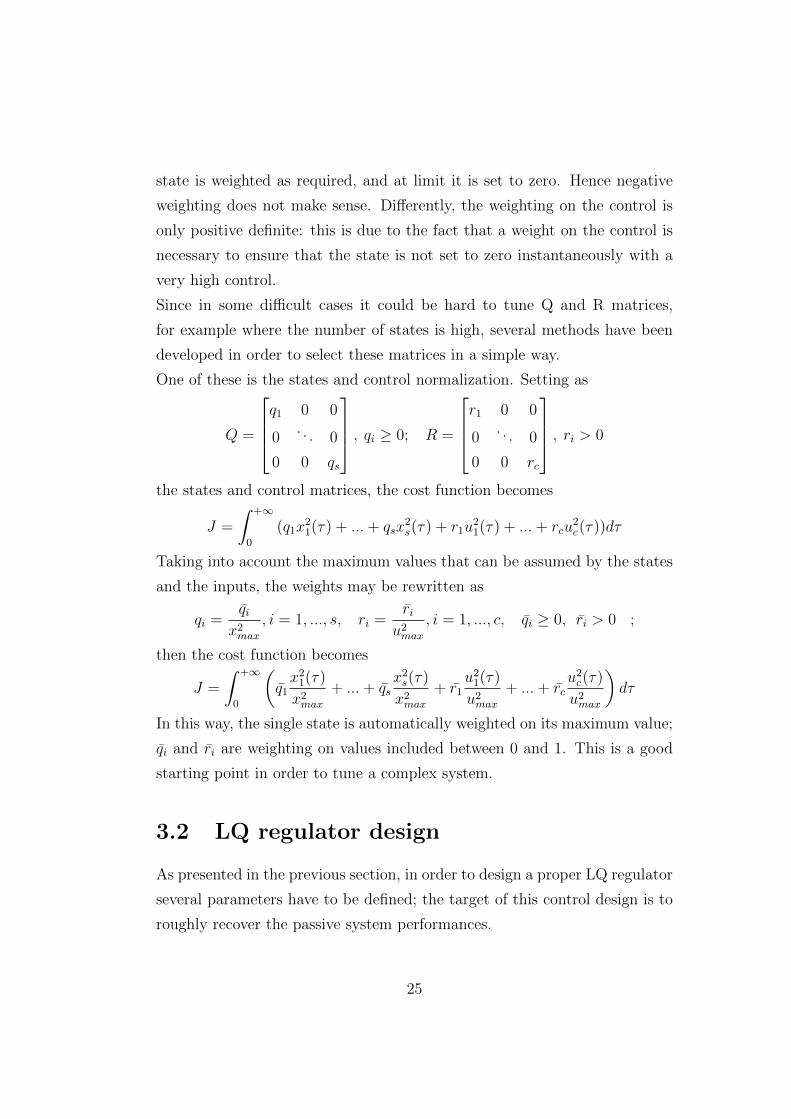
3.1 Anti-yaw damper,secondary yaw control: passive and
active approaches . . . . . . . . . . . . . . . . . . . . 26
3.2 Mechanical model with secondary yaw actuators . . 27
3.3 LQR simulation . . . . . . . . . . . . . . . . . . . . . . 30
3.4 Performances comparison: active and passive lateral
displacements . . . . . . . . . . . . . . . . . . . . . . . 30
4
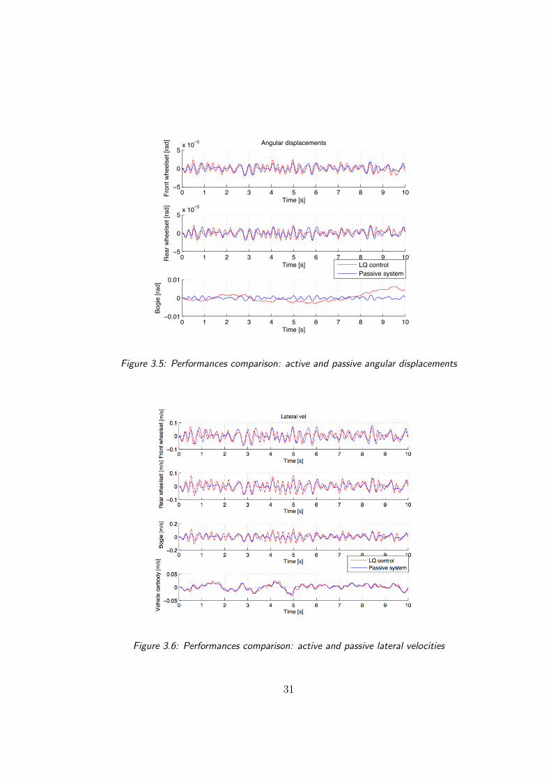
3.5 Performances comparison: active and passive angu-
lar displacements . . . . . . . . . . . . . . . . . . . . . 31
3.6 Performances comparison: active and passive lateral
velocities . . . . . . . . . . . . . . . . . . . . . . . . . . 31
3.7 Performances comparison: active and passive angu-
lar velocities . . . . . . . . . . . . . . . . . . . . . . . . 32
4.1 Sensors configuration on the considered vehicle . . 37
4.2 Simulink model of LQG control . . . . . . . . . . . . 40
4.3 Front wheelset lateral displacement and velocity . 43
4.4 Front wheelset angular displacement and yaw rate . 43
4.5 Rear wheelset lateral displacement and velocity . . 43
4.6 Rear wheelset angular displacement and yaw rate . 44
4.7 Bogie lateral displacement and velocity . . . . . . . 44
4.8 Bogie angular displacement and yaw rate . . . . . . 44
4.9 Carbody lateral displacement and velocity . . . . . . 45
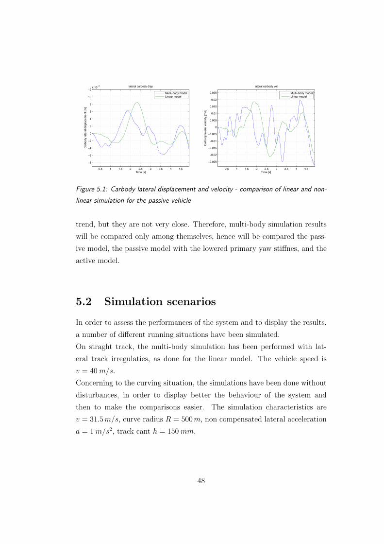
5.1 Carbody lateral displacement and velocity - com-
parison of linear and non-linear simulation for the
passive vehicle . . . . . . . . . . . . . . . . . . . . . . 48
5.2 Passive model with the lowered primary yaw stiff-
ness simulation . . . . . . . . . . . . . . . . . . . . . . 50
5.3 Passive model simulation . . . . . . . . . . . . . . . . 51
5.4 Active model simulation . . . . . . . . . . . . . . . . 51
5.5 Y/Q Ratio comparison . . . . . . . . . . . . . . . . . 53
5.6 Passive model ripage forces . . . . . . . . . . . . . . 54
5.7 Passive model ripage forces with soft p.y.s. . . . . . 55
5.8 Active system ripage forces . . . . . . . . . . . . . . 55
5.9 Power dissipation of the two wheels, passive model 56
5.10 Power dissipation of the two wheels, passive model
with soft p.y.s. . . . . . . . . . . . . . . . . . . . . . . 57
5.11 Power dissipation of the two wheels, active model . 57

List of Tables
2.1 Eigenvalue analysis . . . . . . . . . . . . . . . . . . . . 20
4.1 List of sensors . . . . . . . . . . . . . . . . . . . . . . . 38
5.1 Straight track lateral wheelset acceleration RMS val-
ues comparison . . . . . . . . . . . . . . . . . . . . . . 50
5.2 Energy dissipation on each wheel: the number refers
to the wheelset (i.e. 2=trailing wheelset of the first
bogie), the letter refers to Right or Left wheel . . . 56
Abstract
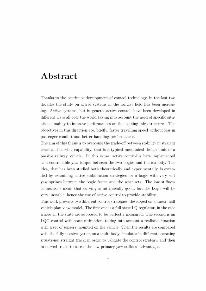
Thanks to the continuos development of control technology, in the last two
decades the study on active systems in the railway field has been increas-
ing. Active systems, but in general active control, have been developed in
different ways all over the world taking into account the need of specific situ-
ations, mainly to improve performances on the existing infrastructures. The
objectives in this direction are, briefly, faster travelling speed without loss in
passenger comfort and better handling performances.
The aim of this thesis is to overcome the trade-off between stability in straight
track and curving capability, that is a typical mechanical design limit of a
passive railway vehicle. In this sense, active control is here implemented
as a controllable yaw torque between the two bogies and the carbody. The
idea, that has been studied both theoretically and experimentally, is exten-
ded by examining active stabilisation strategies for a bogie with very soft
yaw springs between the bogie frame and the wheelsets. The low stiffness
connections mean that curving is intrinsically good, but the bogie will be
very unstable, hence the use of active control to provide stability.
This work presents two different control strategies, developed on a linear, half
vehicle plan view model. The first one is a full state LQ regulator, in the case
where all the state are supposed to be perfectly measured. The second is an
LQG control with state estimation, taking into account a realistic situation
with a set of sensors mounted on the vehicle. Then the results are compared
with the fully passive system on a multi body simulator in different operating
situations: straight track, in order to validate the control strategy, and then
in curved track, to assess the low primary yaw stiffness advantages.
1
Abstract in italiano
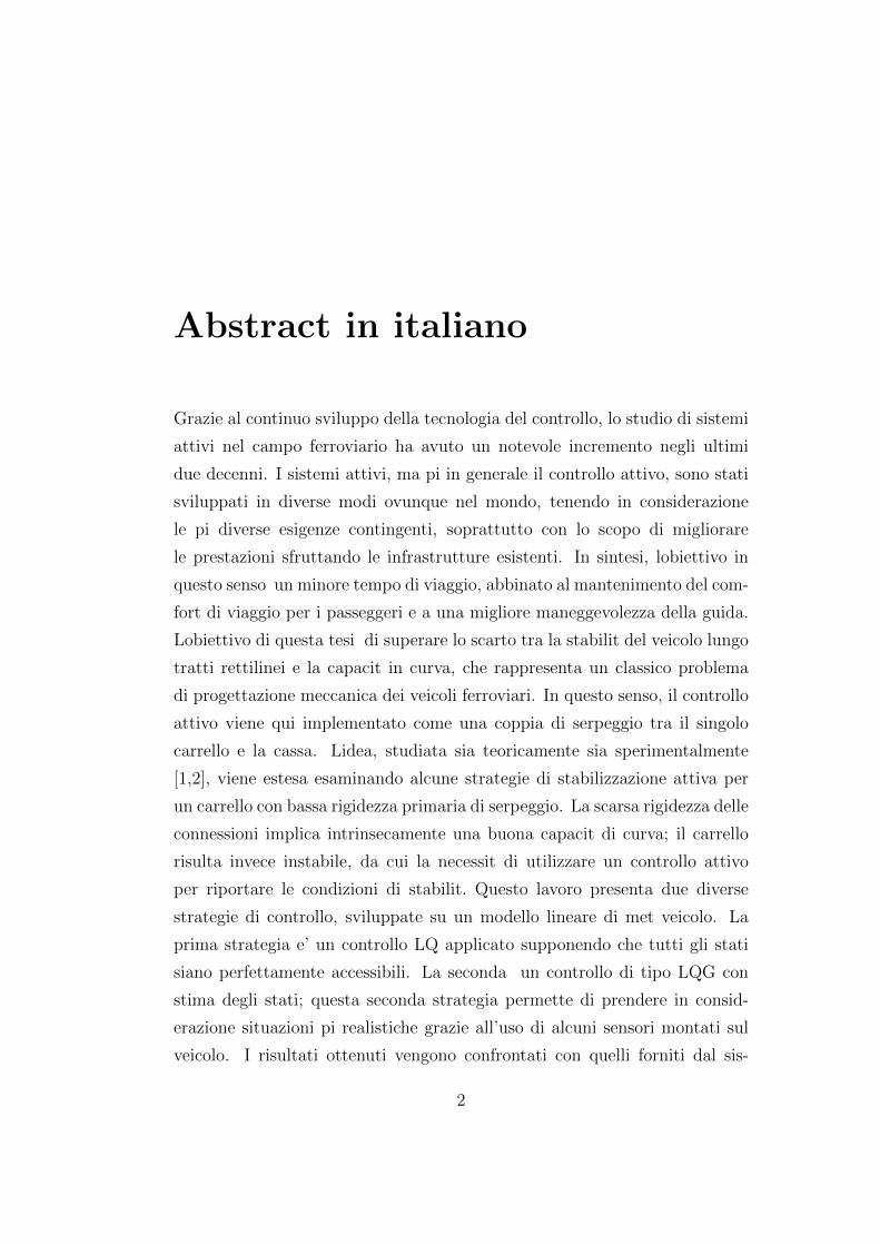
Grazie al continuo sviluppo della tecnologia del controllo, lo studio di sistemi
attivi nel campo ferroviario ha avuto un notevole incremento negli ultimi
due decenni. I sistemi attivi, ma pi in generale il controllo attivo, sono stati
sviluppati in diverse modi ovunque nel mondo, tenendo in considerazione
le pi diverse esigenze contingenti, soprattutto con lo scopo di migliorare
le prestazioni sfruttando le infrastrutture esistenti. In sintesi, lobiettivo in
questo senso un minore tempo di viaggio, abbinato al mantenimento del com-
fort di viaggio per i passeggeri e a una migliore maneggevolezza della guida.
Lobiettivo di questa tesi di superare lo scarto tra la stabilit del veicolo lungo
tratti rettilinei e la capacit in curva, che rappresenta un classico problema
di progettazione meccanica dei veicoli ferroviari. In questo senso, il controllo
attivo viene qui implementato come una coppia di serpeggio tra il singolo
carrello e la cassa. Lidea, studiata sia teoricamente sia sperimentalmente
[1,2], viene estesa esaminando alcune strategie di stabilizzazione attiva per
un carrello con bassa rigidezza primaria di serpeggio. La scarsa rigidezza delle
connessioni implica intrinsecamente una buona capacit di curva; il carrello
risulta invece instabile, da cui la necessit di utilizzare un controllo attivo
per riportare le condizioni di stabilit. Questo lavoro presenta due diverse
strategie di controllo, sviluppate su un modello lineare di met veicolo. La
prima strategia e’ un controllo LQ applicato supponendo che tutti gli stati
siano perfettamente accessibili. La seconda un controllo di tipo LQG con
stima degli stati; questa seconda strategia permette di prendere in consid-
erazione situazioni pi realistiche grazie all’uso di alcuni sensori montati sul
veicolo. I risultati ottenuti vengono confrontati con quelli forniti dal sis-
2
tema su di un simulatore multi-body, operante in diverse situazioni: tratti
con tracciato rettilineo, per validare la strategia di controllo, quindi tratti
curvilinei, al fine di dimostrare i vantaggi della ridotta rigidezza primaria di
serpeggio.

Chapter 1
Introduction
1.1 Preface
In high speed railway vehicles, the use of active control and active systems
has increased in order to overcome certain limits imposed by the mechanical
design. One of the most famous examples is the Pendolino train, developed
by Fiat Ferroviaria in Italy; this is the first example of actively actuated
tilting train.
From this initial and successful idea, different applications of active systems
on railway vehicles have been studied and developed. This trend of replacing
passive components with active systems will continue probably until a radical
mechanical redesign of the railway vehicle will be achieved ([5]). Generally,
active systems pemit to improve the performances of a certain mechanical
system. A typical limit of performances in a railway vehicle is set by the
trade-off between critical speed and dynamic stability. Different solutions
have been studied over the years, in different countries for specific issues res-
olution. When the critical velocity is exceeded, a specific kind of dynamic
instability occours: the hunting instability. Basically, this phenomenon is
caused by the yaw motion of the wheelsets and the bogie, coupled with the
wheel-rail contact (Figure 1.2). Active control is intended to overtake the
velocity limit, ensuring the dynamic stability.
5
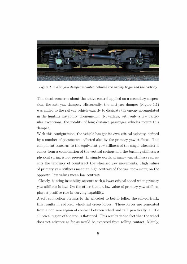
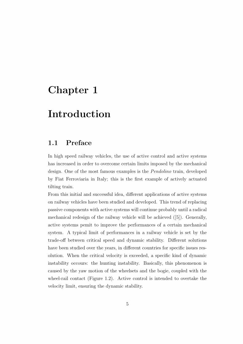
Figure 1.1: Anti yaw damper mounted between the railway bogie and the carbody
This thesis concerns about the active control applied on a secondary suspen-
sion, the anti yaw damper. Historically, the anti yaw damper (Figure 1.1)
was added to the railway vehicle exactly to dissipate the energy accumulated
in the hunting instability phenomenon. Nowadays, with only a few partic-
ular exceptions, the totality of long distance passenger vehicles mount this
damper.
With this configuration, the vehicle has got its own critical velocity, defined
by a number of parameters, affected also by the primary yaw stiffness. This
component concerns to the equivalent yaw stiffness of the single wheelset: it
comes from a combination of the vertical springs and the bushing stiffness; a
physical spring is not present. In simple words, primary yaw stiffness repres-
ents the tendency of counteract the wheelset yaw movements. High values
of primary yaw stiffness mean an high contrast of the yaw movement; on the
opposite, low values mean low contrast.
Clearly, hunting instability occours with a lower critical speed when primary
yaw stiffness is low. On the other hand, a low value of primary yaw stiffness
plays a positive role in curving capability.
A soft connection permits to the wheelset to better follow the curved track:
this results in reduced wheel-rail creep forces. These forces are generated
from a non zero region of contact between wheel and rail; practically, a little
elliptical region of the iron is flattened. This results in the fact that the wheel
does not advance as far as would be expected from rolling contact. Mainly,
6
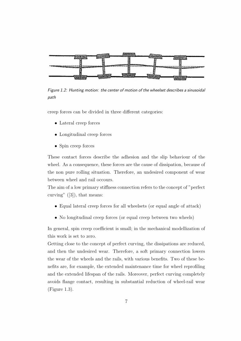
Figure 1.2: Hunting motion: the center of motion of the wheelset describes a sinusoidal
path
creep forces can be divided in three different categories:
• Lateral creep forces
• Longitudinal creep forces
• Spin creep forces
These contact forces describe the adhesion and the slip behaviour of the
wheel. As a consequence, these forces are the cause of dissipation, because of
the non pure rolling situation. Therefore, an undesired component of wear
between wheel and rail occours.
The aim of a low primary stiffness connection refers to the concept of ”perfect
curving” ([3]), that means:
• Equal lateral creep forces for all wheelsets (or equal angle of attack)
• No longitudinal creep forces (or equal creep between two wheels)
In general, spin creep coefficient is small; in the mechanical modellization of
this work is set to zero.
Getting close to the concept of perfect curving, the dissipations are reduced,
and then the undesired wear. Therefore, a soft primary connection lowers
the wear of the wheels and the rails, with various benefits. Two of these be-
nefits are, for example, the extended maintenance time for wheel reprofiling
and the extended lifespan of the rails. Moreover, perfect curving completely
avoids flange contact, resulting in substantial reduction of wheel-rail wear
(Figure 1.3).
7
1
2 3
4
Figure 1.3: Example of wheel wear: on the left, a worn wheel. On the right, the areas
of wear: 1) flange wear 2) tread wear 3) false flange 4) unworn rail. Blue line refers
to an unworn wheel profile
The aim of the thesis concerns the overcoming of this mechanical trade-off:
to reduce the wear through a reduced primary yaw stiffness connection, main-
taining the same critical speed. Since, as previously explained, this situation
carries to a dynamical instability, the proposed solution is the application of
an active control in order to recover the stability situation. In particular, the
active control is applied on the secondary yaw suspention: this appoach is
called ”Secondary Yaw Control” ([3]). Practically, this method is realized re-
placing the anti-yaw dampers with an electric motor equipped with a proper
transmission, that permits to convert the rotational to the linear movement.
The description of these phenomena, in particular the contact forces, could
become difficult when an accurate discussion is needed. In order to avoid
unnecessary complications, the active control strategies have been developed
on a linear model; then, the results have been validated on a multi body non
linear model. In this way, it is possible to evaluate, with a good accurancy,
the creep forces and to compare them in every single situation.
Considering this scenario, an initial guess of primary yaw stiffness reduction
has been done; then, through an appropriate lineal model, the passive and
the active system behaviour has been studied in straight track. Two different
control strategies have been developed, in order to recover a stability condi-
8
tion.
In this thesis, linear optimal control is used for both the control strategies.
This kind of feedback control has been studied and used in various applic-
ations, such as the lateral and the vertical dynamic control of the railway
vehicle ([5]). The same could be said for the state estimation, in particular
the Kalman filter practical application: it has been included in several situ-
ations, where a restricted set of parameters are measured, and sensors and
process noises are taken into account; an example could be found in [9].
Historically, active suspensions appear in the first part of the 20th century
as research and development work on various automotive vehicles. Active
control on railway vehicles was introduced mainly to operate on the same
infrastructure of other trains. For example, Pendolino train was able to op-
erate at curving speed around 15% higher than conventional trains. This
improvement is obtained by the active tilting of the carbody, that allows to
reduce the non compensed trasversal acceleration due to the cant deficiency.
Therefore, in railway tracks rich in tight curves as for the Italian tracks, this
system permits to increase the average trip velocity, and then to reduce the
travelling time ([7])
A practical application of the Secondary Yaw Control can be found in [2],
where line tests with a high speed vehicle have been performed. This study
is probably the closest application of Secondary yaw control that this thesis
proposes to do. Other research informations on Secondary yaw control can
be found in [6].
1.2 Thesis structure
The thesis is structured in the following parts:
• in Chapter 2 the mathematical model of the railway vehicle taken into
account will be presented; the equations of motion and the related state
space model will be computed. Moreover, a stability overview will be
9
assessed.
• in Chapter 3 the LQ optimal control will be studied and applied on the
linear model; the choice of the regulator weights will be discussed and
a result comparison with the passive model will be performed.
• in Chapter 4 the LQG control and the Kalman filter design will be
presented. Considerations on the sensors will be done, and a compar-
ison between the passive model and the two control strategies will be
displayed.
• in Chapter 5 a multi body non linear simulator is taken into account,
and the railway vehicle will be simulated in this environment. Several
comparisons with the previous simulations will be done, and the final
aim of the thesis will be assessed.
• in Chapter 6 the entire work will be summarized and will be presen-
ted the possible developments, in term of control strategy design and
simulation/validation methods.
• in Appendix A the physical parameters of the linear mechanical model
will be listed.
10
Chapter 2
Mathematical model for
straight track
2.1 System description
A typical modern-style vehicle is taken into account in order to study the dy-
namic response and then develop the control strategies. This kind of model
has got several peculiarities that could be summarized in three aspects: lin-
ear, half vehicle, plan view. Generally, a mathematical model is focused on
describing reasonably the reality, and at the same time to be simple enough
to permit a proper control strategy development. Physically, the model is
composed by four rigid bodies: two wheelsets, a bogie and half carbody, in-
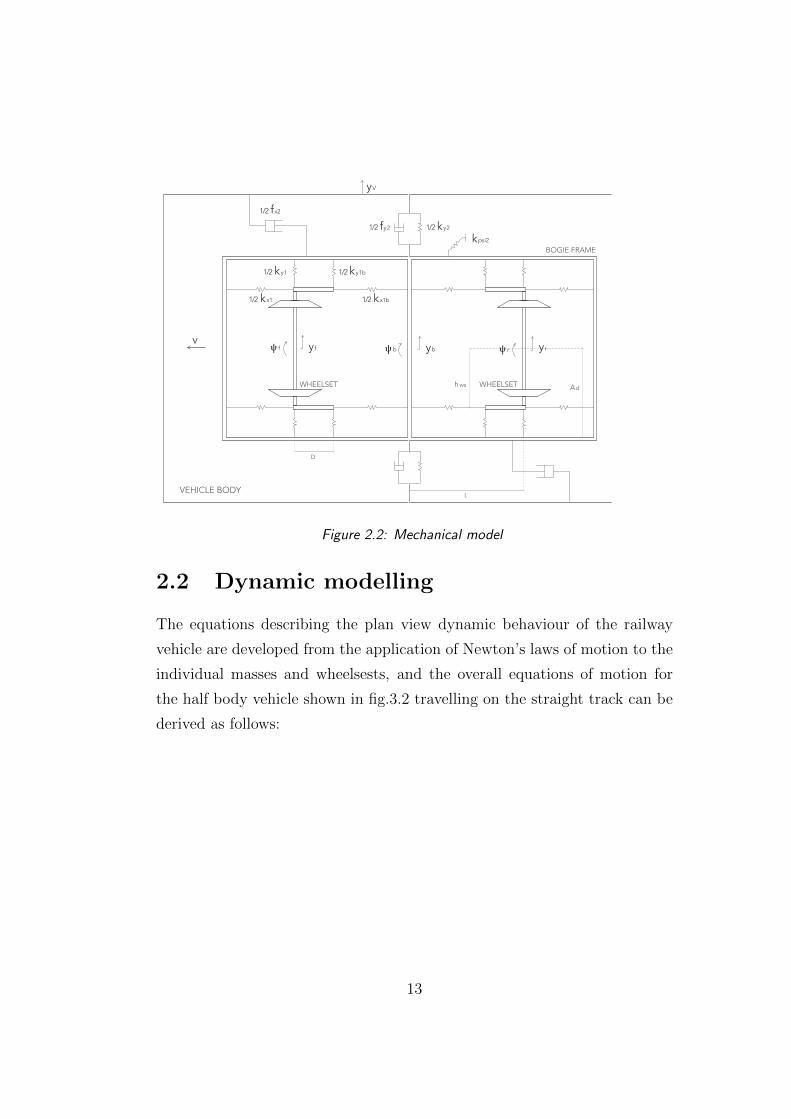
terconnected by dampers and springs. The mechanical arrangement is shown
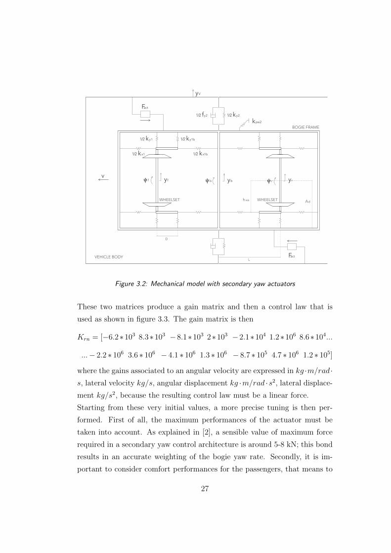
in fig. 3.2.
Below the major assumptions are pointed out, explaining how they have been
addressed.
2.1.1 Linear model
The dynamic behaviour of a railway vehicle, in general, shows different types
of non-linearities; one of these is the wheel-rail contact. As explained by
various authors ([1]), this mechanism is described by the creep forces (also
11
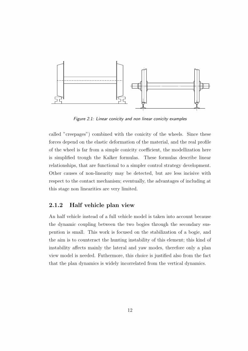
Figure 2.1: Linear conicity and non linear conicity examples
called ”creepages”) combined with the conicity of the wheels. Since these
forces depend on the elastic deformation of the material, and the real profile
of the wheel is far from a simple conicity coefficient, the modellization here
is simplified trough the Kalker formulas. These formulas describe linear
relationships, that are functional to a simpler control strategy development.
Other causes of non-linearity may be detected, but are less incisive with
respect to the contact mechanism; eventually, the advantages of including at
this stage non linearities are very limited.
2.1.2 Half vehicle plan view
An half vehicle instead of a full vehicle model is taken into account because
the dynamic coupling between the two bogies through the secondary sus-
pention is small. This work is focused on the stabilization of a bogie, and
the aim is to counteract the hunting instability of this element; this kind of
instability affects mainly the lateral and yaw modes, therefore only a plan
view model is needed. Futhermore, this choice is justified also from the fact
that the plan dynamics is widely incorrelated from the vertical dynamics.
12
1/2 1/2
fx2
fy2 ky2
k psi2
D
VEHICLE BODY
WHEELSET WHEELSET
BOGIE FRAME
L
Ad
1/2
1/2
1/2
1/2k
y
y1
ψ f f
yV
yψ b b
h ws
yψ r r
k y1b
k
v
x1 1/2 k x1b
Figure 2.2: Mechanical model
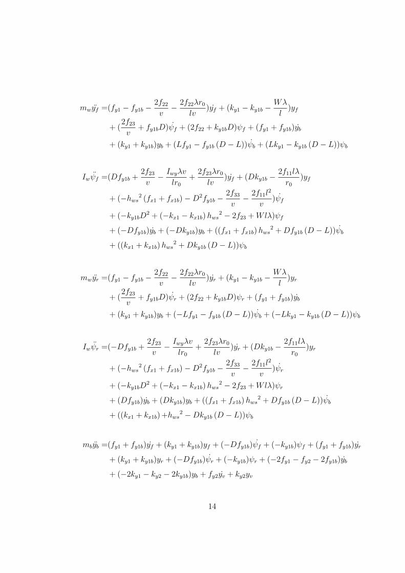
2.2 Dynamic modelling
The equations describing the plan view dynamic behaviour of the railway
vehicle are developed from the application of Newton’s laws of motion to the
individual masses and wheelsests, and the overall equations of motion for
the half body vehicle shown in fig.3.2 travelling on the straight track can be
derived as follows:
13
mwyf =(fy1 − fy1b −2f22v− 2f22λr0
lv)yf + (ky1 − ky1b −
Wλ
l)yf
+ (2f23v
+ fy1bD)ψf + (2f22 + ky1bD)ψf + (fy1 + fy1b)yb
+ (ky1 + ky1b)yb + (Lfy1 − fy1b (D − L))ψb + (Lky1 − ky1b (D − L))ψb
Iwψf =(Dfy1b +2f23v− Iwyλv
lr0+
2f23λr0lv
)yf + (Dky1b −2f11lλ
r0)yf
+ (−hws2 (fx1 + fx1b)−D2fy1b −2f33v− 2f11l
2
v)ψf
+ (−ky1bD2 + (−kx1 − kx1b)hws2 − 2f23 +Wlλ)ψf
+ (−Dfy1b)yb + (−Dky1b)yb + ((fx1 + fx1b)hws2 +Dfy1b (D − L))ψb
+ ((kx1 + kx1b)hws2 +Dky1b (D − L))ψb
mwyr =(fy1 − fy1b −2f22v− 2f22λr0
lv)yr + (ky1 − ky1b −
Wλ
l)yr
+ (2f23v
+ fy1bD)ψr + (2f22 + ky1bD)ψr + (fy1 + fy1b)yb
+ (ky1 + ky1b)yb + (−Lfy1 − fy1b (D − L))ψb + (−Lky1 − ky1b (D − L))ψb
Iwψr =(−Dfy1b +2f23v− Iwyλv
lr0+
2f23λr0lv
)yr + (Dky1b −2f11lλ
r0)yr
+ (−hws2 (fx1 + fx1b)−D2fy1b −2f33v− 2f11l
2
v)ψr
+ (−ky1bD2 + (−kx1 − kx1b)hws2 − 2f23 +Wlλ)ψr
+ (Dfy1b)yb + (Dky1b)yb + ((fx1 + fx1b)hws2 +Dfy1b (D − L))ψb
+ ((kx1 + kx1b) +hws2 −Dky1b (D − L))ψb
mbyb =(fy1 + fy1b)yf + (ky1 + ky1b)yf + (−Dfy1b)ψf + (−ky1b)ψf + (fy1 + fy1b)yr
+ (ky1 + ky1b)yr + (−Dfy1b)ψr + (−ky1b)ψr + (−2fy1 − fy2 − 2fy1b)yb
+ (−2ky1 − ky2 − 2ky1b)yb + fy2yv + ky2yv
14
Ibψb =(Lfy1 −Dfy1b − fy1b (D − L))yf + (Lky1 −Dky1b − ky1b (D − L))yf
+ (hws2 (fx1 + fx1b) +D2fy1b +Dfy1b (D − L))ψf
+ (hws2 (kx1 + kx1b) +D2ky1b +Dky1b (D − L))ψf
+ (Dfy1b − Lfy1 + fy1b (D − L))yr + (Dky1b − Lky1 + ky1b (D − L))yr
+ (hws2 (fx1 + fx1b) +D2fy1b +Dfy1b (D − L))ψr
+ (hws2 (kx1 + kx1b) +D2ky1b +Dky1b (D − L))ψr
+ (−2hws2 (fx1 + fx1b)− Ad2fx2 − 2L2fy1 − 2fy1b(D − L)2 − 2Dfy1b (D − L))ψb
+ (−2hws2 (kx1 + kx1b)− kψ2 − 2L2ky1 − 2ky1b(D − L)2 − 2Dky1b (D − L))ψb
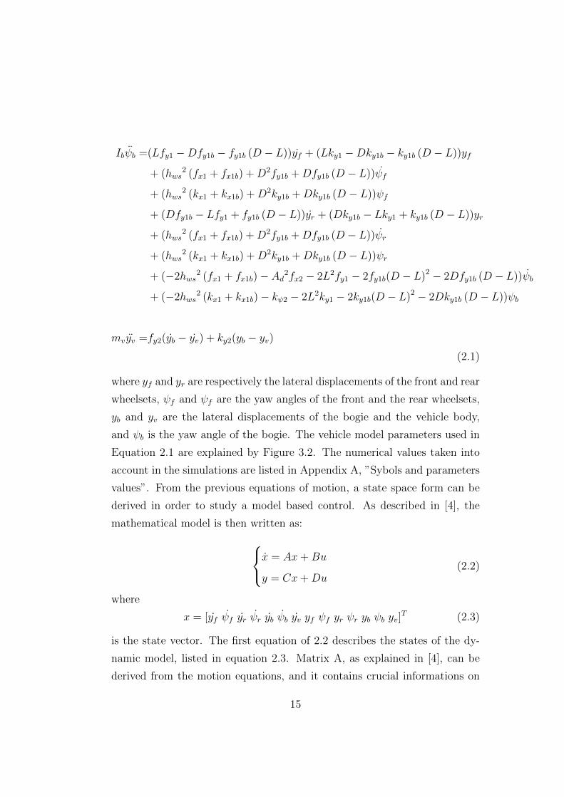
mvyv =fy2(yb − yv) + ky2(yb − yv)(2.1)
where yf and yr are respectively the lateral displacements of the front and rear
wheelsets, ψf and ψf are the yaw angles of the front and the rear wheelsets,
yb and yv are the lateral displacements of the bogie and the vehicle body,
and ψb is the yaw angle of the bogie. The vehicle model parameters used in
Equation 2.1 are explained by Figure 3.2. The numerical values taken into
account in the simulations are listed in Appendix A, ”Sybols and parameters
values”. From the previous equations of motion, a state space form can be
derived in order to study a model based control. As described in [4], the
mathematical model is then written as:x = Ax+Bu
y = Cx+Du(2.2)
where
x = [yf ψf yr ψr yb ψb yv yf ψf yr ψr yb ψb yv]T (2.3)
is the state vector. The first equation of 2.2 describes the states of the dy-
namic model, listed in equation 2.3. Matrix A, as explained in [4], can be
derived from the motion equations, and it contains crucial informations on
15
the stability of the system. At this stage, B matrix, that defines the inputs
that affect the system, is not present; afterwards, when a control action will
be defined, B matrix will be added to the model.
The second equation of 2.2 describes the measurements performed on the
system; these are defined by the sensors mounted on the train. In particular,
C matrix concerns the sensors arrangement; this part will be explained better
in Chapter 4, ”Sensing assessment”. Matrix D, as for matrix B, is not present
because there is not direct transfer between inputs and measurements.
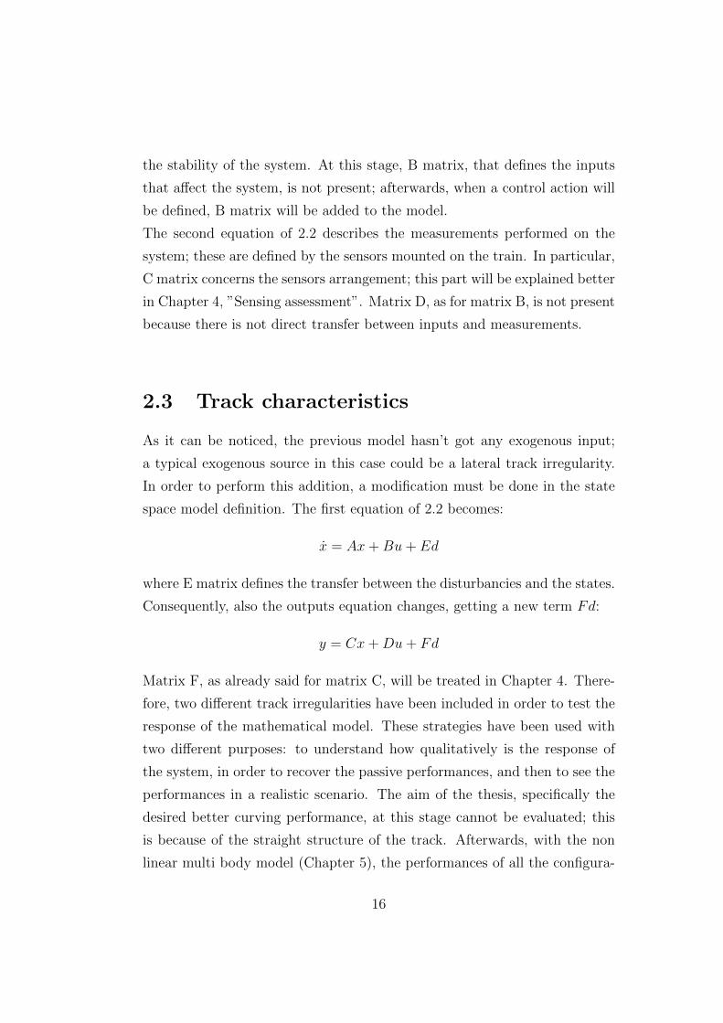
2.3 Track characteristics
As it can be noticed, the previous model hasn’t got any exogenous input;
a typical exogenous source in this case could be a lateral track irregularity.
In order to perform this addition, a modification must be done in the state
space model definition. The first equation of 2.2 becomes:
x = Ax+Bu+ Ed
where E matrix defines the transfer between the disturbancies and the states.
Consequently, also the outputs equation changes, getting a new term Fd:
y = Cx+Du+ Fd
Matrix F, as already said for matrix C, will be treated in Chapter 4. There-
fore, two different track irregularities have been included in order to test the
response of the mathematical model. These strategies have been used with
two different purposes: to understand how qualitatively is the response of
the system, in order to recover the passive performances, and then to see the
performances in a realistic scenario. The aim of the thesis, specifically the
desired better curving performance, at this stage cannot be evaluated; this
is because of the straight structure of the track. Afterwards, with the non
linear multi body model (Chapter 5), the performances of all the configura-
16
0 0.2 0.4 0.6 0.8 1 1.2 1.4 1.6 1.8 2−5
0
5
10
15x 10−3
Time [s]
Late
ral s
tep
[m]
Figure 2.3: Example of lateral step disturbance, 0.01 m
tions will be studied.
Below a detailed analysis of the two straight track strategies is presented.
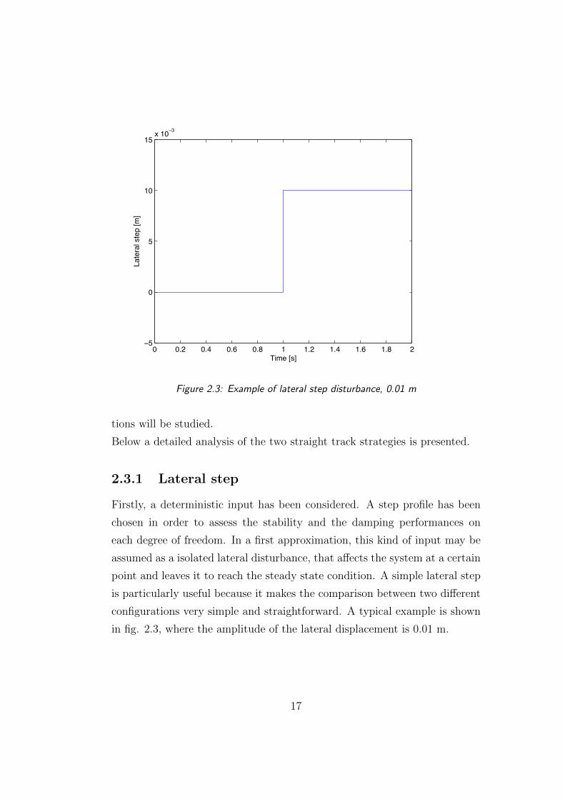
2.3.1 Lateral step
Firstly, a deterministic input has been considered. A step profile has been
chosen in order to assess the stability and the damping performances on
each degree of freedom. In a first approximation, this kind of input may be
assumed as a isolated lateral disturbance, that affects the system at a certain
point and leaves it to reach the steady state condition. A simple lateral step
is particularly useful because it makes the comparison between two different
configurations very simple and straightforward. A typical example is shown
in fig. 2.3, where the amplitude of the lateral displacement is 0.01 m.
17
0 100 200 300 400 500 600 700 800 900 1000−0.015
−0.01
−0.005
0
0.005
0.01
0.015
Distance traveled [m]
Late
ral d
ispl
acem
ent [
m]
Figure 2.4: Example of lateral measured disturbance
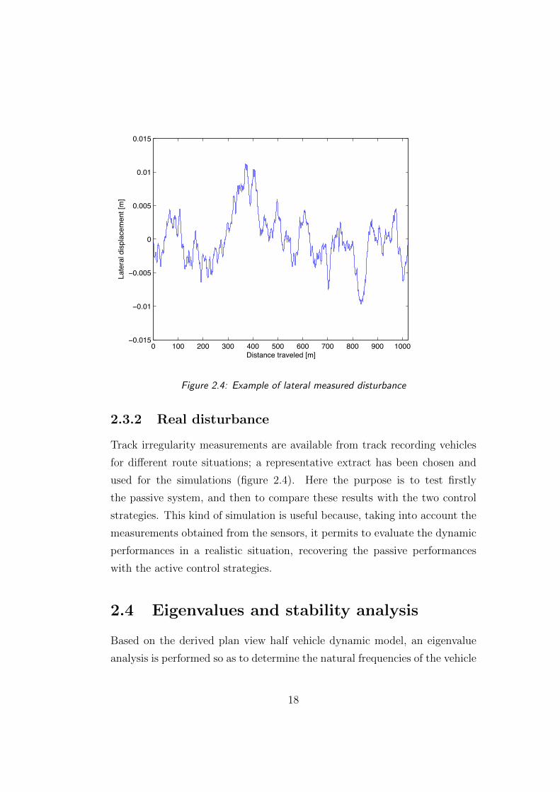
2.3.2 Real disturbance
Track irregularity measurements are available from track recording vehicles
for different route situations; a representative extract has been chosen and
used for the simulations (figure 2.4). Here the purpose is to test firstly
the passive system, and then to compare these results with the two control
strategies. This kind of simulation is useful because, taking into account the
measurements obtained from the sensors, it permits to evaluate the dynamic
performances in a realistic situation, recovering the passive performances
with the active control strategies.
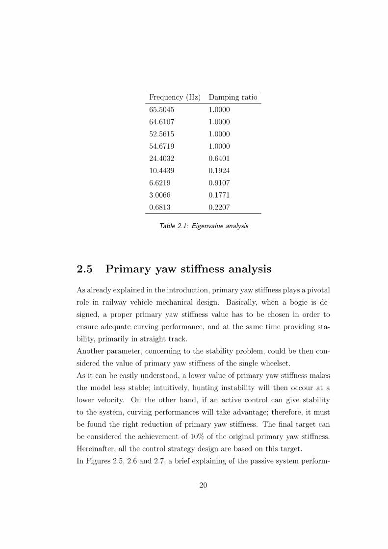
2.4 Eigenvalues and stability analysis
Based on the derived plan view half vehicle dynamic model, an eigenvalue
analysis is performed so as to determine the natural frequencies of the vehicle
18
dynamic modes and the damping ratios associated with each mode; the res-
ults are shown in table 2.1. The analysis has been performed with the numer-
ical values listed in Appendix A. It can be seen that a few kinematic modes
are shown; these are the ones that display a frequency below 10 Hz and a
damping ratio lower than 1. In order to evaluate the stability of the system,
these two parameters are taken into account: in particular, when a damping
ratio becomes negative, this is related to an unstable mode. In other words,
this means that the associated eigenvalue has reached positive real part.
In the model that has been taken into account several parameters affect the
running performances and the resulting stability. The most important are
two: λ, linear conicity coefficient and v, vehicle forward velocity. As a first
analysis, it can be said that velocity and conicity are inversely proportional
to the stability: the more these values increase, the less the vehicle is stable.
In fact, as it can be seen in the equations of motion, when they become lar-
ger, they both concur to decrease the damping contribution in the lateral and
yaw dynamics of the wheelsets. In general, the damping contribution helps
to dissipate the energy of the system. When this value becomes lower, and
in the worst case negative, this means that the system is not dissipating all
the energy that is gaining, and when it is negative it is feeding the instability
phenomenon. This is why hunting instability occours: a linear model shows
that conicity and velocity are closely related to this issue.
In practice, using the lateral step input, several simulations have been per-
formed in order to test the dynamic response of the system.
19
Frequency (Hz) Damping ratio
65.5045 1.0000
64.6107 1.0000
52.5615 1.0000
54.6719 1.0000
24.4032 0.6401
10.4439 0.1924
6.6219 0.9107
3.0066 0.1771
0.6813 0.2207
Table 2.1: Eigenvalue analysis
2.5 Primary yaw stiffness analysis
As already explained in the introduction, primary yaw stiffness plays a pivotal
role in railway vehicle mechanical design. Basically, when a bogie is de-
signed, a proper primary yaw stiffness value has to be chosen in order to
ensure adequate curving performance, and at the same time providing sta-
bility, primarily in straight track.
Another parameter, concerning to the stability problem, could be then con-
sidered the value of primary yaw stiffness of the single wheelset.
As it can be easily understood, a lower value of primary yaw stiffness makes
the model less stable; intuitively, hunting instability will then occour at a
lower velocity. On the other hand, if an active control can give stability
to the system, curving performances will take advantage; therefore, it must
be found the right reduction of primary yaw stiffness. The final target can
be considered the achievement of 10% of the original primary yaw stiffness.
Hereinafter, all the control strategy design are based on this target.
In Figures 2.5, 2.6 and 2.7, a brief explaining of the passive system perform-
20

0 0.5 1 1.5 2 2.5 3
−0.25
−0.2
−0.15
−0.1
−0.05
0
0.05
0.1
0.15
0.2
0.25
Time [s]
Fron
t whe
else
t yaw
rate
[rad
/s]
0 0.5 1 1.5 2 2.5 3
−0.25
−0.2
−0.15
−0.1
−0.05
0
0.05
0.1
0.15
0.2
0.25
Time [s]
Fron
t whe
else
t yaw
rate
[rad
/s]
Figure 2.5: v = 40 m/s and v = 50 m/s, λ=0.15, p.y.s.=100%
0 0.5 1 1.5 2 2.5 3
−0.25
−0.2
−0.15
−0.1
−0.05
0
0.05
0.1
0.15
0.2
0.25
Time [s]
Fron
t whe
else
t yaw
rate
[rad
/s]
0 0.5 1 1.5 2 2.5 3
−0.25
−0.2
−0.15
−0.1
−0.05
0
0.05
0.1
0.15
0.2
0.25
Time [s]
Fron
t whe
else
t yaw
rate
[rad
/s]
Figure 2.6: v = 40 m/s and v = 50 m/s, λ=0.25, p.y.s.=100%
ances is proposed. The results are displayed in two different ways: a time
history and a eigenvalue plot. The time history is referred to a single de-
gree of freedom, specifically the yaw rate of the front wheelset, v = 40m/s,
forced with a step input, 0.01 m of amplitude; concerning to the eigenvalues,
a negative damping means an unstable mode.
21

0 0.5 1 1.5 2 2.5 3
−0.25
−0.2
−0.15
−0.1
−0.05
0
0.05
0.1
0.15
0.2
0.25
Time [s]
Fron
t whe
else
t yaw
rate
[rad
/s]
0 0.5 1 1.5 2 2.5 3
−0.25
−0.2
−0.15
−0.1
−0.05
0
0.05
0.1
0.15
0.2
0.25
Time [s]
Fron
t whe
else
t yaw
rate
[rad
/s]
Figure 2.7: v = 40 m/s, λ=0.25, p.y.s.=50% and p.y.s.=10%
22
Chapter 3
LQR control
3.1 Introduction
In this chapter an application of a full state optimal control is presented.
Firstly, the linear quadratic optimal control theory is discussed, and then it
is implemented in this case, as explained in Chapter 1, ”Introduction”.
Optimal control has been applied in various fields of automotive problems,
such as active suspensions in automobiles, but also in the railway branch.
Here, this kind of control is taken into account in order to overcome the
trade-off between stability and curving performances, as discussed before.
Below the first optimal control strategy is presented, an LQ full state regu-
lator; afterwards another control strategy will be presented, an LQG control
with state estimation. These two strategies could be considered as classical
approaches of optimal control: these have been taken into account as logical
beginning of a state-based control. Possible developments in this field will
be discussed in Chapter 6, ”Conclusions”.
3.1.1 Linear Quadratic optimal control (LQ)
The control method, as generally for optimal control, is obtained from an
appropriate problem of optimization in time domain. In this way, in the
formulation of the control it is possible to include potential constraints on
23
the state and control variables; these are defined by the weights that can
be found in the cost function. LQ control deals with linear quadratic cost
functions.
Considering a linear, time invariant system where the state is accessible,
x(t) = Ax(t) +Bu(t)
is the state equation. Concerning to the figure of merit,
J(x0, u, 0) =
∫ +∞
0
(x′(τ)Qx(τ) + u′(τ)Ru(τ))dτ (3.1)
is the linear quadratic formula, where
Q = Q′ ≥ 0, R = R′ > 0
are design parameters. Q and R matrix are almost always diagonal, but there
is no specific form restriction. Taking into account the Riccati differential
equation,
P = A′P + PA+Q− PBR−1B′P = 0 (3.2)
and the associated linear control law,
u = −R−1B′Px = −Krx
subject to (A,B) controllable, (A,Cq) observable, and Q is constructed as
Q = C ′qCq. Kr is the matrix that minimises the cost function written in 3.1.
In 3.2, P has been set to zero because the optimization problem is considered
on a infinite horizon. This control law is time-invariant and it does not need
the knowledge of the current state; therefore, it can be computed a priori.
3.1.2 LQR tuning
The optimization of the figure of merit is made through the state weighting
matrix Q and the control weighting matrix R, that allow to weight the single
state and the control action, respectively. It is interesting to note that the
weighting on the states is positive semi-definite, that is sensible: a single
24
state is weighted as required, and at limit it is set to zero. Hence negative
weighting does not make sense. Differently, the weighting on the control is
only positive definite: this is due to the fact that a weight on the control is
necessary to ensure that the state is not set to zero instantaneously with a
very high control.
Since in some difficult cases it could be hard to tune Q and R matrices,
for example where the number of states is high, several methods have been
developed in order to select these matrices in a simple way.
One of these is the states and control normalization. Setting as
Q =
q1 0 0
0. . . 0
0 0 qs
, qi ≥ 0; R =
r1 0 0
0. . . 0
0 0 rc
, ri > 0
the states and control matrices, the cost function becomes
J =
∫ +∞
0
(q1x21(τ) + ...+ qsx
2s(τ) + r1u
21(τ) + ...+ rcu
2c(τ))dτ
Taking into account the maximum values that can be assumed by the states
and the inputs, the weights may be rewritten as
qi =qi
x2max, i = 1, ..., s, ri =
riu2max
, i = 1, ..., c, qi ≥ 0, ri > 0 ;
then the cost function becomes
J =
∫ +∞
0
(q1x21(τ)
x2max+ ...+ qs
x2s(τ)
x2max+ r1
u21(τ)
u2max+ ...+ rc
u2c(τ)
u2max
)dτ
In this way, the single state is automatically weighted on its maximum value;
qi and ri are weighting on values included between 0 and 1. This is a good
starting point in order to tune a complex system.
3.2 LQ regulator design
As presented in the previous section, in order to design a proper LQ regulator
several parameters have to be defined; the target of this control design is to
roughly recover the passive system performances.
25
Figure 3.1: Anti-yaw damper,secondary yaw control: passive and active approaches
3.2.1 Weights tuning
Since in this case the state vector contains 14 variables, the first weighting
attempt is done with the state normalization. The maximum values as-
sumed by the states have been obtaned from a number of simulations on the
passive model; it is important to note that these simulations are performed
on the linear system, with the original value of primary yaw stiffness. In
some cases the assumption of linearity, especially for large deflection of the
springs/dampers, gives results that are not reliable, because the simulation
could deviate sensibly from the reality. Practically, taking into account re-
corded lateral track disturbancies, the maximum value of the single state has
been measured, and then used in the Q matrix. Concerning to the R matrix,
it has been considered the damper on the passive model, in particular the
maximum force exerted by this element. Therefore, the weights associated to
an angular velocity are expressed in s2/rad2, lateral velocity s2/m2, angular
displacement 1/rad2, lateral displacement 1/m2, input force 1/N2. Below
this first attempt is displayed, remembering also the state vector.
x = [yf ψf yr ψr yb ψb yv yf ψf yr ψr yb ψb yv]T (3.3)
Qn = diag[38, 1.79∗102, 57, 1.04∗102, 41, 1.96∗102, 92, 1.16∗103, 6.92∗104, ...
...4, 96 ∗ 103, 5.17 ∗ 104, 4.5 ∗ 103, 7.71 ∗ 104, 2.83 ∗ 103]
R = [1.29 ∗ 10−9]
26
1/2 1/2
Fact
Fact
fy2 ky2
k psi2
D
VEHICLE BODY
WHEELSET WHEELSET
BOGIE FRAME
L
Ad
1/2
1/2
1/2k
y
y1
ψ f f
yV
yψ b b
h ws
yψ r r
k y1b
k
v
x1 1/2 k x1b
Figure 3.2: Mechanical model with secondary yaw actuators
These two matrices produce a gain matrix and then a control law that is
used as shown in figure 3.3. The gain matrix is then
Krn = [−6.2∗103 8.3∗103 −8.1∗103 2∗103 −2.1∗104 1.2∗106 8.6∗104...
...− 2.2 ∗ 106 3.6 ∗ 106 − 4.1 ∗ 106 1.3 ∗ 106 − 8.7 ∗ 105 4.7 ∗ 106 1.2 ∗ 105]
where the gains associated to an angular velocity are expressed in kg ·m/rad·s, lateral velocity kg/s, angular displacement kg ·m/rad ·s2, lateral displace-
ment kg/s2, because the resulting control law must be a linear force.
Starting from these very initial values, a more precise tuning is then per-
formed. First of all, the maximum performances of the actuator must be
taken into account. As explained in [2], a sensible value of maximum force
required in a secondary yaw control architecture is around 5-8 kN; this bond
results in an accurate weighting of the bogie yaw rate. Secondly, it is im-
portant to consider comfort performances for the passengers, that means to
27
keep under a sensible threshold the accelerations of the system. In general,
large values of velocities and accelerations on the states of the model are un-
desired because the mechanical parts, for example spring or dampers, have
got physical limits that cannot be overcome. Hence, the values assumed from
the passive system are a suitable term of comparison. Below the adjusted
weights in the Q matrix.
Q = Qn · [1 1 1 1 1 15 1 0.1 1 0.1 1 1 1 0.1]T
The associated gain matrix becomes
Kr = Krn · diag[1.02, 0.32, 0.62, 0.14, 1.14, 3.65, 0.56, ...
...0.7, 0.45, 0.71, 0.37, 0.54, 0.86, 0.1] (3.4)
With this setting, the maximum force exerted by the motor is 7.6 kN, that
is an acceptable value. It is interesting to notice that, both in the Q matrix
and Kr array, the value associated to the bogie yaw rate differs visibly from
the other values. This is due to the fact that in Q matrix the associated
weight has to be high enough to not exceed the maximum force of the motor;
in the gain array, it points out that the bogie yaw rate is the most import-
ant component used in the feedback. Intuitively, this is correct because in
the passive situation the anti-yaw damper works only on the bogie yaw rate,
therefore it is the most important component.
3.2.2 Active control actuator
At this point, it is important to show where the active control acts into the
equations of the system. The yaw damper, the mechanical device that coun-
teracts the action of hunting instability, affects the equation of momenta of
the bogie. Therefore, in the active system this component must be elimin-
ated. Active control replaces the function of this mechanical part using an
electric drive. Practically, the motor must be placed in the same position
of the damper, and through a transmission the rotational movement of the
28
motor is converted to a linear motion, as shown in figure 3.1. Here all the
mechanical dynamics of the motor, for reason of simplicity, are not taken
into account; the only parameter that has been considered is the maximum
force that can be exerted by the motor.
Therefore, in order to include the actuator in the mathematical model, B
matrix has been used to define the control input.
With these informations, a number of simulations have been performed, in
order to validate the stability of the new mechanical system with the lowered
primary yaw stiffness; in the next section the results will be displayed.
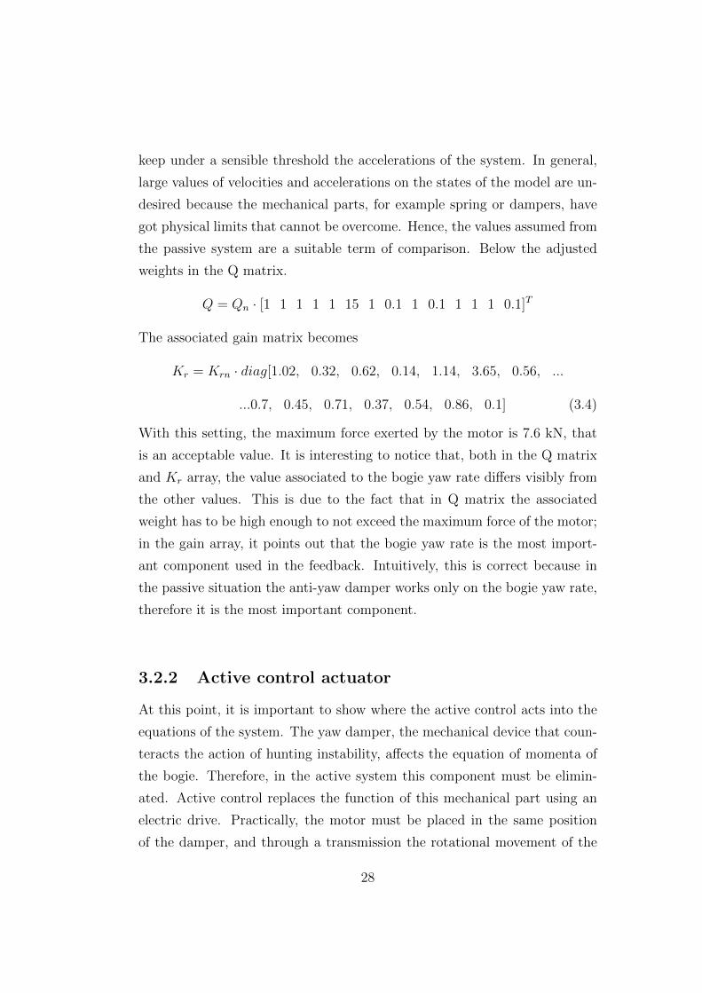
3.3 Linear simulation
Here some sample demonstrations of the control strategy are shown. In
Figure 3.3 the simulation structure can be seen, and it is composed by:
• lateral track disturbance that acts on the front and the rear wheelsets
• state space model that describes the system
• feedback with the LQR gain array
• full state measurement
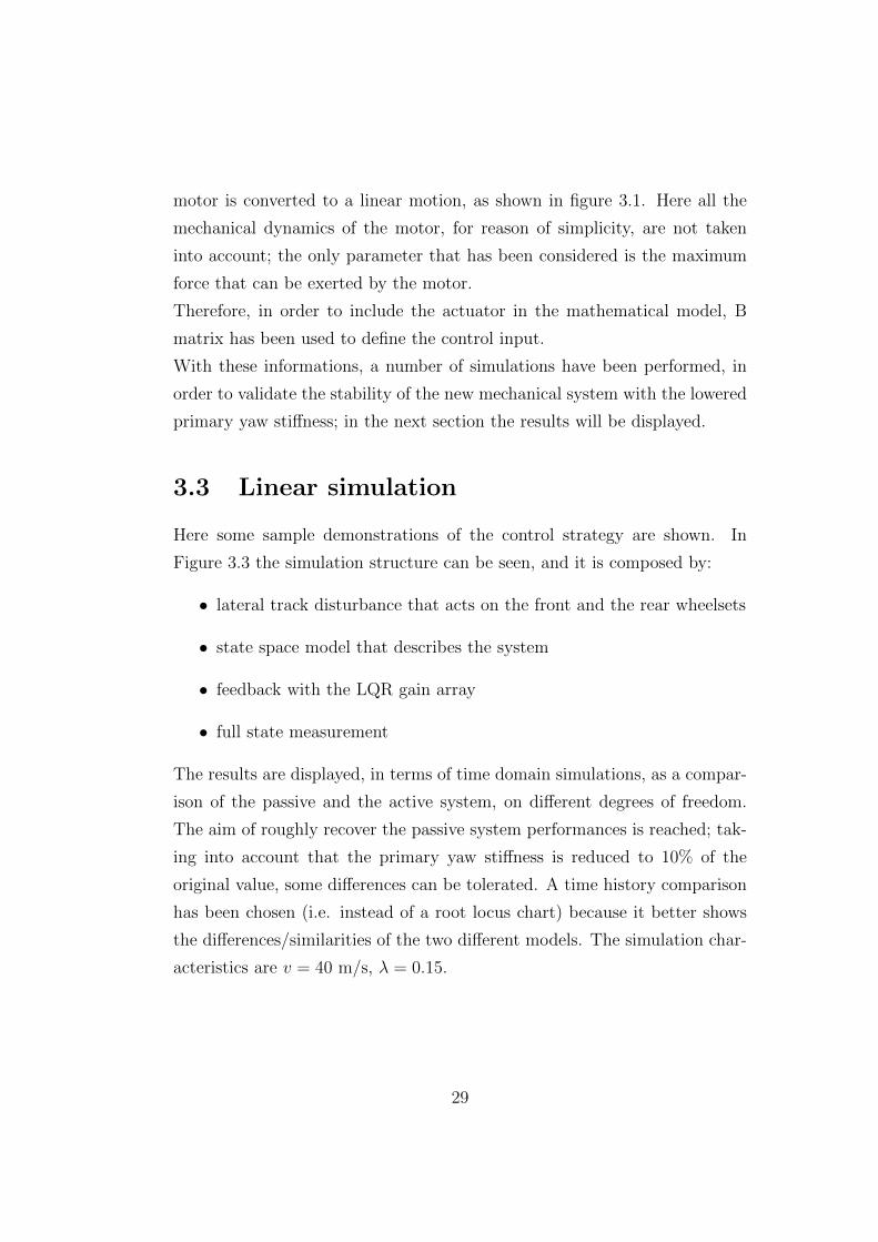
The results are displayed, in terms of time domain simulations, as a compar-
ison of the passive and the active system, on different degrees of freedom.
The aim of roughly recover the passive system performances is reached; tak-
ing into account that the primary yaw stiffness is reduced to 10% of the
original value, some differences can be tolerated. A time history comparison
has been chosen (i.e. instead of a root locus chart) because it better shows
the differences/similarities of the two different models. The simulation char-
acteristics are v = 40 m/s, λ = 0.15.
29
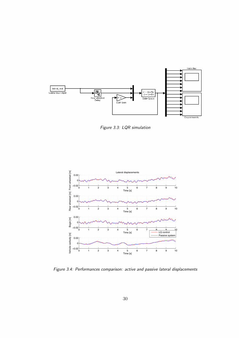
Figure 3.3: LQR simulation
0 1 2 3 4 5 6 7 8 9 10−0.02
0
0.02
Time [s]Fron
t whe
else
t [m
]
Lateral displacements
0 1 2 3 4 5 6 7 8 9 10−0.02
0
0.02
Time [s]Rea
r whe
else
t [m
]
0 1 2 3 4 5 6 7 8 9 10−0.02
0
0.02
Time [s]
Bogi
e [m
]
0 1 2 3 4 5 6 7 8 9 10−0.02
0
0.02
Time [s]Vehi
cle
carb
ody
[m]
LQ controlPassive system
Figure 3.4: Performances comparison: active and passive lateral displacements
30
0 1 2 3 4 5 6 7 8 9 10−5
0
5x 10⁻³
Time [s]
Fron
t whe
else
t [ra
d] Angular displacements
0 1 2 3 4 5 6 7 8 9 10−5
0
5x 10⁻³
Time [s]
Rea
r whe
else
t [ra
d]
0 1 2 3 4 5 6 7 8 9 10−0.01
0
0.01
Time [s]
Bogi
e [ra
d]
LQ controlPassive system
Figure 3.5: Performances comparison: active and passive angular displacements
Figure 3.6: Performances comparison: active and passive lateral velocities
31
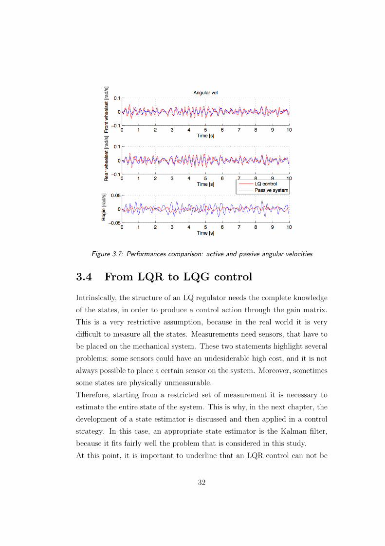
Figure 3.7: Performances comparison: active and passive angular velocities
3.4 From LQR to LQG control
Intrinsically, the structure of an LQ regulator needs the complete knowledge
of the states, in order to produce a control action through the gain matrix.
This is a very restrictive assumption, because in the real world it is very
difficult to measure all the states. Measurements need sensors, that have to
be placed on the mechanical system. These two statements highlight several
problems: some sensors could have an undesiderable high cost, and it is not
always possible to place a certain sensor on the system. Moreover, sometimes
some states are physically unmeasurable.
Therefore, starting from a restricted set of measurement it is necessary to
estimate the entire state of the system. This is why, in the next chapter, the
development of a state estimator is discussed and then applied in a control
strategy. In this case, an appropriate state estimator is the Kalman filter,
because it fits fairly well the problem that is considered in this study.
At this point, it is important to underline that an LQR control can not be
32

a realistic solution of the problem, especially in this case, where a railway
vehicle is taken into account. However this control strategy has been de-
veloped because it constitutes the natural first step for an optimal control,
and above all it is a term of comparison for the control with state estimation.
33
Chapter 4
LQG control with sensing
assessment
4.1 Introduction
As explained in the previous chapter, a Linear Quadratic Gaussian control
has been developed. In this chapter the structure of this control strategy is
firstly shown, and then implemented on the system. LQG control is obtained
from an LQ control law in combination with a Kalman filter, that is used to
get the estimation of the states where the system is affected by stochastic
disturbances.
This kind of control strategy could be considered as an evolution compared
to the LQ approach, because it takes into account more realistically the cir-
cumstances in which the system is inserted. In order to produce an LQ regu-
lator, a full knowledge of the states is needed; this assumption is particularly
strong where the system owns a considerable number of degrees of freedom.
Moreover, measurements are inevitably affected by noise and errors, that
must be taken into account; the system can be also affected by disturbances.
LQG control takes into account the issues listed above, because the purpose
of the Kalman filter is precisely to estimate the entire state of the system
with a restricted set of measurements affected by noise. It is important to
34
note that the control is called ”Gaussian”: the model disturbances and the
measurement noises must be modeled as Gaussian white noises.
4.1.1 Kalman filter
The Kalman filter is a state obsever with optimality peculiarities, that must
be implemented when the system is affected by stochastic disturbances. Con-
sidering the linear system x = Ax+Bu+ vx
y = Cx+ vy(4.1)
where vx is the process noise and vy is the measurements noise; these are
uncorrelated gaussian white noises with zero mean, and covariance matrix V
defined as
v =
[vx
vy
], E[v(t)] = 0, E[v(t1)v(t2)
′] = V δ(t1 − t2)
V =
[Q 0
0 R
]where δ is the Kroenecker index. Noises on the states and on the output are
assumed to be uncorrelated.
Therefore, the observer taken into account is
˙x(t) = Ax(t) +Bu(t) + L(t)[y(t)− Cx(t)]
where L(t) is a time variant gain chosen to meet an optimality criterion. As
already explained for the LQ control, a time invariant law can be produced:
˙x(t) = Ax(t) +Bu(t) + L[y(t)− y(t)] = Ax(t) +Bu(t) + L[y(t)− Cx(t)] =
= (A− LC)x(t) +Bu(t) + Ly(t) (4.2)
where
L = PC ′R−1
35
with P is the unique definite positive solution of the Riccati equation
0 = A′P + PA+ Q− PC ′R−1CP (4.3)
This result is subjected to (C,A) observable, Q ≥ 0, and (A,Bq) controllable,
where Q = BqB′q. The estimator thus obtained is asimptotically stable,
because the eigenvalues of (A− LC) have negative real part.
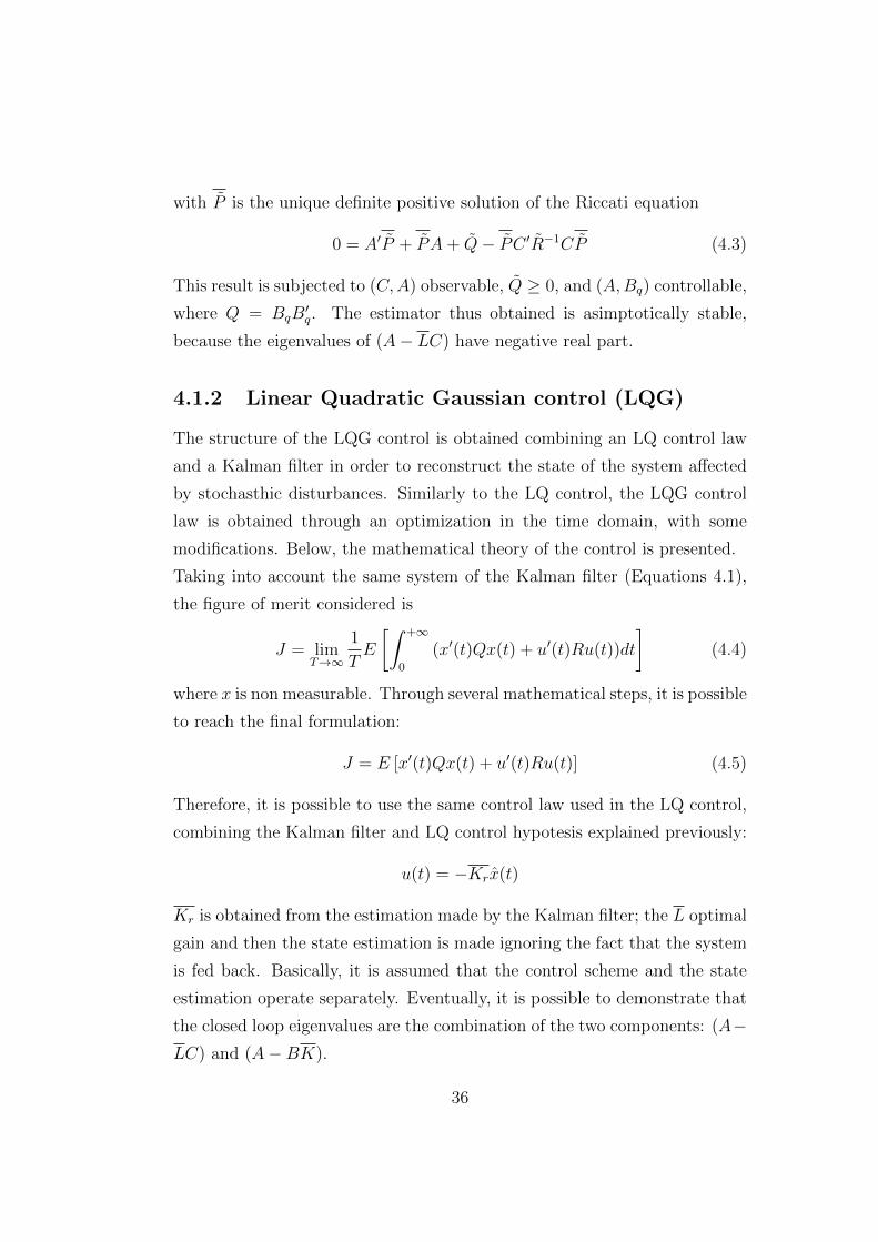
4.1.2 Linear Quadratic Gaussian control (LQG)
The structure of the LQG control is obtained combining an LQ control law
and a Kalman filter in order to reconstruct the state of the system affected
by stochasthic disturbances. Similarly to the LQ control, the LQG control
law is obtained through an optimization in the time domain, with some
modifications. Below, the mathematical theory of the control is presented.
Taking into account the same system of the Kalman filter (Equations 4.1),
the figure of merit considered is
J = limT→∞
1
TE
[∫ +∞
0
(x′(t)Qx(t) + u′(t)Ru(t))dt
](4.4)
where x is non measurable. Through several mathematical steps, it is possible
to reach the final formulation:
J = E [x′(t)Qx(t) + u′(t)Ru(t)] (4.5)
Therefore, it is possible to use the same control law used in the LQ control,
combining the Kalman filter and LQ control hypotesis explained previously:
u(t) = −Krx(t)
Kr is obtained from the estimation made by the Kalman filter; the L optimal
gain and then the state estimation is made ignoring the fact that the system
is fed back. Basically, it is assumed that the control scheme and the state
estimation operate separately. Eventually, it is possible to demonstrate that
the closed loop eigenvalues are the combination of the two components: (A−LC) and (A−BK).
36
1/2 1/2
Fact
Fact
fy2 ky2
k psi2
D
VEHICLE BODY
WHEELSET WHEELSET
BOGIE FRAME
L
Ad
1/2
1/2
1/2k
A B
C
y
y1
ψ f f
yV
yψ b b
hws
yψ r r
k y1b
k
v
x1 1/2 k x1b
D
E
F
G
H
H
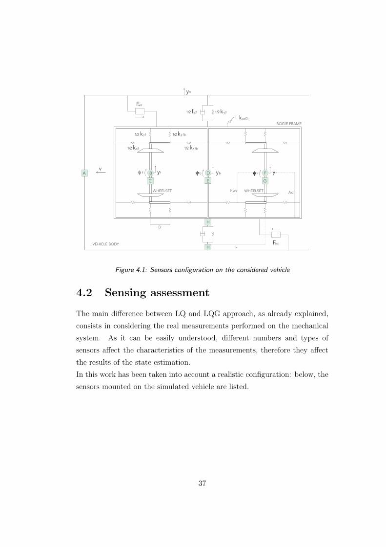
Figure 4.1: Sensors configuration on the considered vehicle
4.2 Sensing assessment
The main difference between LQ and LQG approach, as already explained,
consists in considering the real measurements performed on the mechanical
system. As it can be easily understood, different numbers and types of
sensors affect the characteristics of the measurements, therefore they affect
the results of the state estimation.
In this work has been taken into account a realistic configuration: below, the
sensors mounted on the simulated vehicle are listed.
37
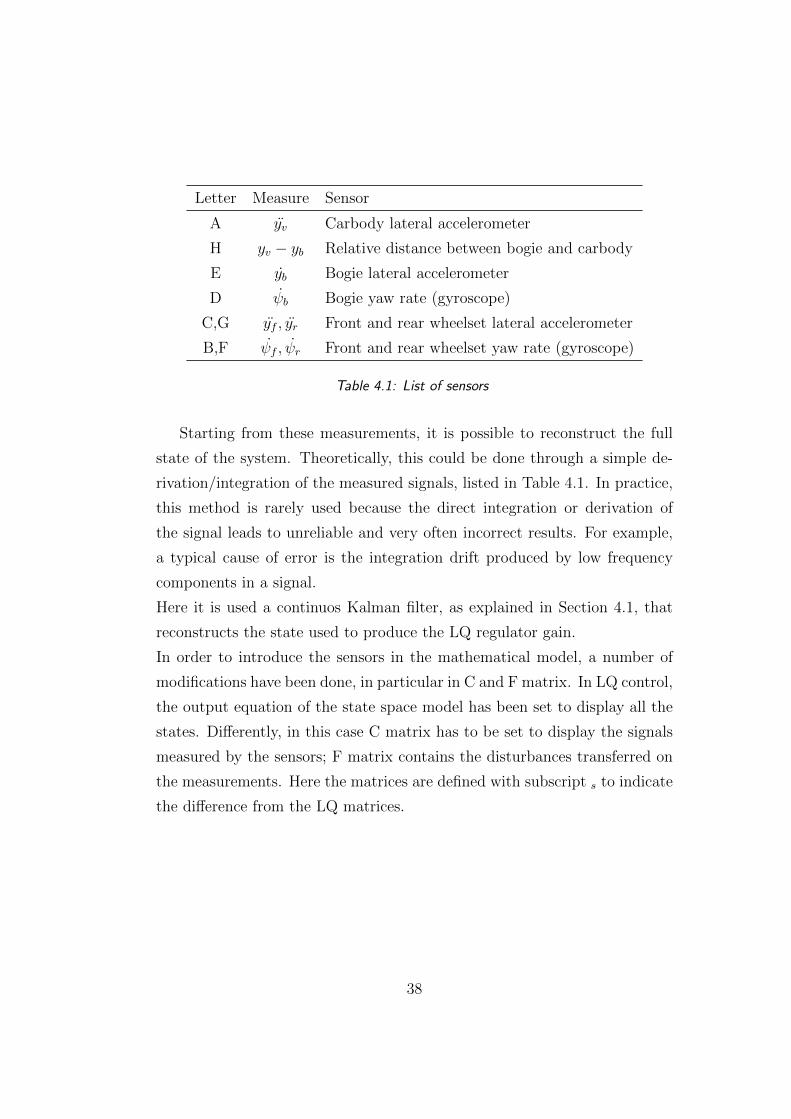
Letter Measure Sensor
A yv Carbody lateral accelerometer
H yv − yb Relative distance between bogie and carbody
E yb Bogie lateral accelerometer
D ψb Bogie yaw rate (gyroscope)
C,G yf , yr Front and rear wheelset lateral accelerometer
B,F ψf , ψr Front and rear wheelset yaw rate (gyroscope)
Table 4.1: List of sensors
Starting from these measurements, it is possible to reconstruct the full
state of the system. Theoretically, this could be done through a simple de-
rivation/integration of the measured signals, listed in Table 4.1. In practice,
this method is rarely used because the direct integration or derivation of
the signal leads to unreliable and very often incorrect results. For example,
a typical cause of error is the integration drift produced by low frequency
components in a signal.
Here it is used a continuos Kalman filter, as explained in Section 4.1, that
reconstructs the state used to produce the LQ regulator gain.
In order to introduce the sensors in the mathematical model, a number of
modifications have been done, in particular in C and F matrix. In LQ control,
the output equation of the state space model has been set to display all the
states. Differently, in this case C matrix has to be set to display the signals
measured by the sensors; F matrix contains the disturbances transferred on
the measurements. Here the matrices are defined with subscript s to indicate
the difference from the LQ matrices.
38
Cs =
A(7, ·)0 0 0 0 0 0 0 0 0 0 0 1 0 − 1
A(5, ·)0 0 0 0 0 1 0 0 0 0 0 0 0 0
A(1, ·)A(3, ·)
0 1 0 0 0 0 0 0 0 0 0 0 0 0
0 0 0 1 0 0 0 0 0 0 0 0 0 0
, Fs =
0 0
0 0
0 0
0 0
E(1, ·)E(3, ·)
0 0
0 0
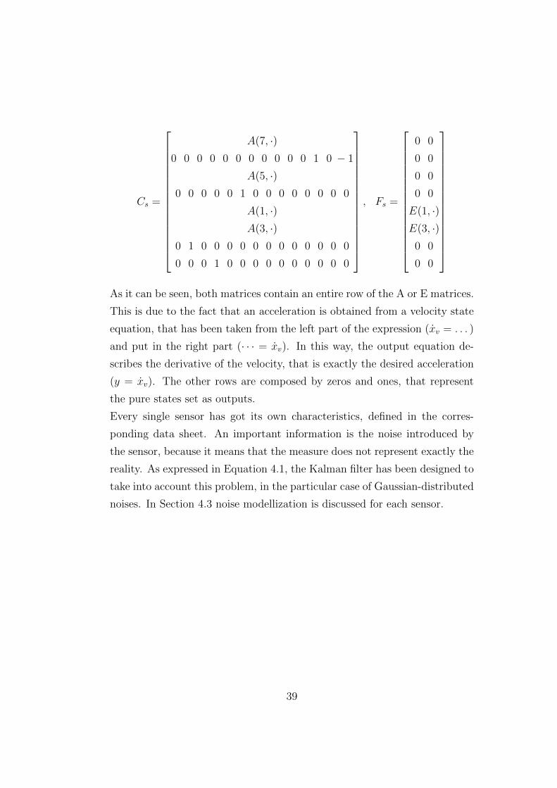
As it can be seen, both matrices contain an entire row of the A or E matrices.
This is due to the fact that an acceleration is obtained from a velocity state
equation, that has been taken from the left part of the expression (xv = . . . )
and put in the right part (· · · = xv). In this way, the output equation de-
scribes the derivative of the velocity, that is exactly the desired acceleration
(y = xv). The other rows are composed by zeros and ones, that represent
the pure states set as outputs.
Every single sensor has got its own characteristics, defined in the corres-
ponding data sheet. An important information is the noise introduced by
the sensor, because it means that the measure does not represent exactly the
reality. As expressed in Equation 4.1, the Kalman filter has been designed to
take into account this problem, in the particular case of Gaussian-distributed
noises. In Section 4.3 noise modellization is discussed for each sensor.
39
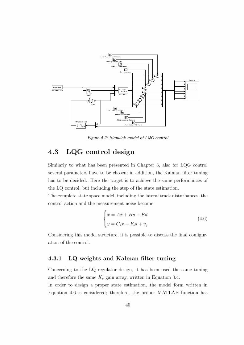
Figure 4.2: Simulink model of LQG control
4.3 LQG control design
Similarly to what has been presented in Chapter 3, also for LQG control
several parameters have to be chosen; in addition, the Kalman filter tuning
has to be decided. Here the target is to achieve the same performances of
the LQ control, but including the step of the state estimation.
The complete state space model, including the lateral track disturbances, the
control action and the measurement noise becomex = Ax+Bu+ Ed
y = Csx+ Fsd+ vy(4.6)
Considering this model structure, it is possible to discuss the final configur-
ation of the control.
4.3.1 LQ weights and Kalman filter tuning
Concerning to the LQ regulator design, it has been used the same tuning
and therefore the same Kr gain array, written in Equation 3.4.
In order to design a proper state estimation, the model form written in
Equation 4.6 is considered; therefore, the proper MATLAB function has
40
been chosen. The function that fits the considered problem is lqew, because
it is based exacly on the state space written in Equation 4.6. This function
needs specific inputs, that are basically the informations needed by a Kalman
filter built on these equations. E[γ] is intended to be the expected value of
γ, differently from E, disturbancies matrix on the state equation.
Below, the input information needed for the state estimation are listed:
• E[dd′] = Q, lateral disturbancies covariance
• E[vv′] = R, sensors noise covariance
• A,Cs, E, Fs, matrices of the state space model
From this information, the Kalman filter gain L is computed, and then the
full state is reconstructed.
˙x = Ax(t) +Bu(t) + L[y − Cx]
The Q matrix has been simply calculed as the variance of the lateral disturb-
ancies signal used in the simulation. The result, used in the simulation, is
1.4235 ∗ 10−5m2. Of course, this value depends on the characteristichs of the
disturbance: since a limited examples of disturbancies have been used, the
variance is calculated a priori, and then put in the simulation. In order to
avoid this limitation, it could be done a variance average on several files of
lateral disturbancies, in order to reach a reliable and general value.
As regards the R matrix, it has to be taken into account the noise of the
single sensor. Practically, as it can be seen in Figure 4.2, a Gaussian white
noise has been added to the measure, with a precise value of variance. This
value has been assumed to be the 1% of the full scale of the sensor. Below,
the variances of each sensor are listed:
• wheelset lateral accelerometer: 3.6 ∗ 10−3m2/s4
• bogie lateral accelerometer: 2.5 ∗ 10−3m2/s4
• carbody lateral accelerometer: 1.6 ∗ 10−3m2/s4
41
• wheelset yaw rate gyroscope: 2.89 ∗ 10−6rad2/s2
• bogie yaw rate gyroscope: 1.44 ∗ 10−6rad2/s2
• lateral distance between bogie and carbody: 4 ∗ 10−6m2
Considering these parameters, a number of simulations have been performed,
in order to validate the control strategy. In Section 4.4 the results are dis-
played and compared with the LQ control strategy, as an ideal term of ref-
erence.
4.4 Linear simulation
As for the LQ control, the aim is to roughly recover the passive system per-
formances; primary yaw stiffness is still reduced to the 10% of the original
passive model value.
Moreover, it is interesting to compare these results with the LQ results, be-
cause the differences represent the validity of the Kalman estimation. Below,
a number of simulation are presented, focusing on the perfomances degrad-
ation caused by the state estimation.
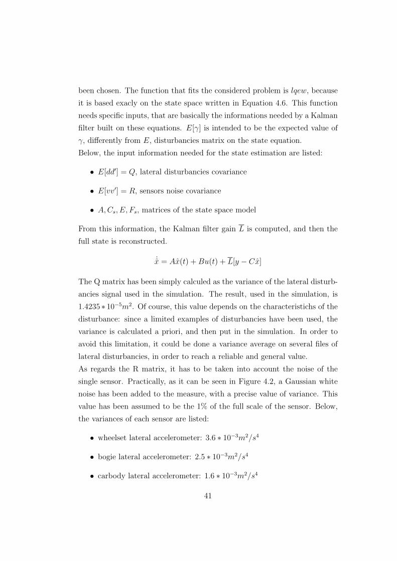
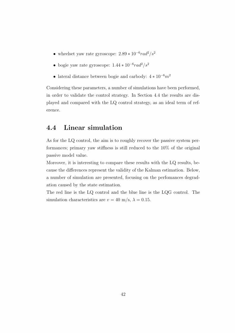
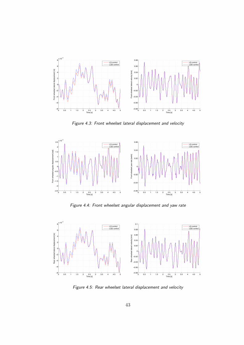
The red line is the LQ control and the blue line is the LQG control. The
simulation characteristics are v = 40 m/s, λ = 0.15.
42
0 0.5 1 1.5 2 2.5 3 3.5 4 4.5 5−8
−6
−4
−2
0
2
4
6
8x 10⁻³
Time [s]
Fron
t whe
else
t lat
eral
dis
plac
emen
t [m
]
LQ controlLQG control
0 0.5 1 1.5 2 2.5 3 3.5 4 4.5 5−0.08
−0.06
−0.04
−0.02
0
0.02
0.04
0.06
0.08
Time [s]
Fron
t whe
else
t lat
eral
vel
ocity
[m/s
]
LQ controlLQG control
Figure 4.3: Front wheelset lateral displacement and velocity
0 0.5 1 1.5 2 2.5 3 3.5 4 4.5 5−2.5
−2
−1.5
−1
−0.5
0
0.5
1
1.5
2
2.5x 10⁻³
Time [s]
Fron
t whe
else
t ang
ular
dis
plac
emen
t [ra
d]
LQ controlLQG control
0 0.5 1 1.5 2 2.5 3 3.5 4 4.5 5−0.06
−0.04
−0.02
0
0.02
0.04
0.06
Time [s]
Fron
t whe
else
t yaw
rate
[rad
/s]
LQ controlLQG control
Figure 4.4: Front wheelset angular displacement and yaw rate
0 0.5 1 1.5 2 2.5 3 3.5 4 4.5 5−8
−6
−4
−2
0
2
4
6
8x 10⁻³
Time [s]
Rea
r whe
else
t lat
eral
dis
plac
emen
t [m
]
LQ controlLQG control
0 0.5 1 1.5 2 2.5 3 3.5 4 4.5 5−0.08
−0.06
−0.04
−0.02
0
0.02
0.04
0.06
0.08
0.1
Time [s]
Rea
r whe
else
t lat
eral
vel
ocity
[m/s
]
LQ controlLQG control
Figure 4.5: Rear wheelset lateral displacement and velocity
43
0 0.5 1 1.5 2 2.5 3 3.5 4 4.5 5−2
−1.5
−1
−0.5
0
0.5
1
1.5
2
2.5x 10⁻³
Time [s]
Rea
r whe
else
t ang
ular
dis
plac
emen
t [ra
d]
LQ controlLQG control
0 0.5 1 1.5 2 2.5 3 3.5 4 4.5 5−0.06
−0.04
−0.02
0
0.02
0.04
0.06
Time [s]
Rea
r whe
else
t yaw
rate
[rad
/s]
LQ controlLQG control
Figure 4.6: Rear wheelset angular displacement and yaw rate
0 0.5 1 1.5 2 2.5 3 3.5 4 4.5 5−10
−8
−6
−4
−2
0
2
4
6
8x 10⁻³
Time [s]
Bogi
e la
tera
l dis
plac
emen
t [m
]
LQ controlLQG control
0 0.5 1 1.5 2 2.5 3 3.5 4 4.5 5−0.2
−0.15
−0.1
−0.05
0
0.05
0.1
0.15
Time [s]
Bogi
e la
tera
l vel
ocity
[m/s
]
LQ controlLQG control
Figure 4.7: Bogie lateral displacement and velocity
0 0.5 1 1.5 2 2.5 3 3.5 4 4.5 5−3
−2
−1
0
1
2
3
4x 10⁻³
Time [s]
Bogi
e an
gula
r dis
plac
emen
t [ra
d]
LQ controlLQG control
0 0.5 1 1.5 2 2.5 3 3.5 4 4.5 5−0.015
−0.01
−0.005
0
0.005
0.01
0.015
Time [s]
Bogi
e ya
w ra
te [r
ad/s
]
LQ controlLQG control
Figure 4.8: Bogie angular displacement and yaw rate
44
0 0.5 1 1.5 2 2.5 3 3.5 4 4.5 5−8
−6
−4
−2
0
2
4
6
8
10x 10−3
Time [s]
Car
body
late
ral d
ispl
acem
ent [
m]
LQ controlLQG control
0 0.5 1 1.5 2 2.5 3 3.5 4 4.5 5−0.04
−0.03
−0.02
−0.01
0
0.01
0.02
0.03
Time [s]
Car
body
late
ral v
eloc
ity [m
/s]
LQ controlLQG control
Figure 4.9: Carbody lateral displacement and velocity
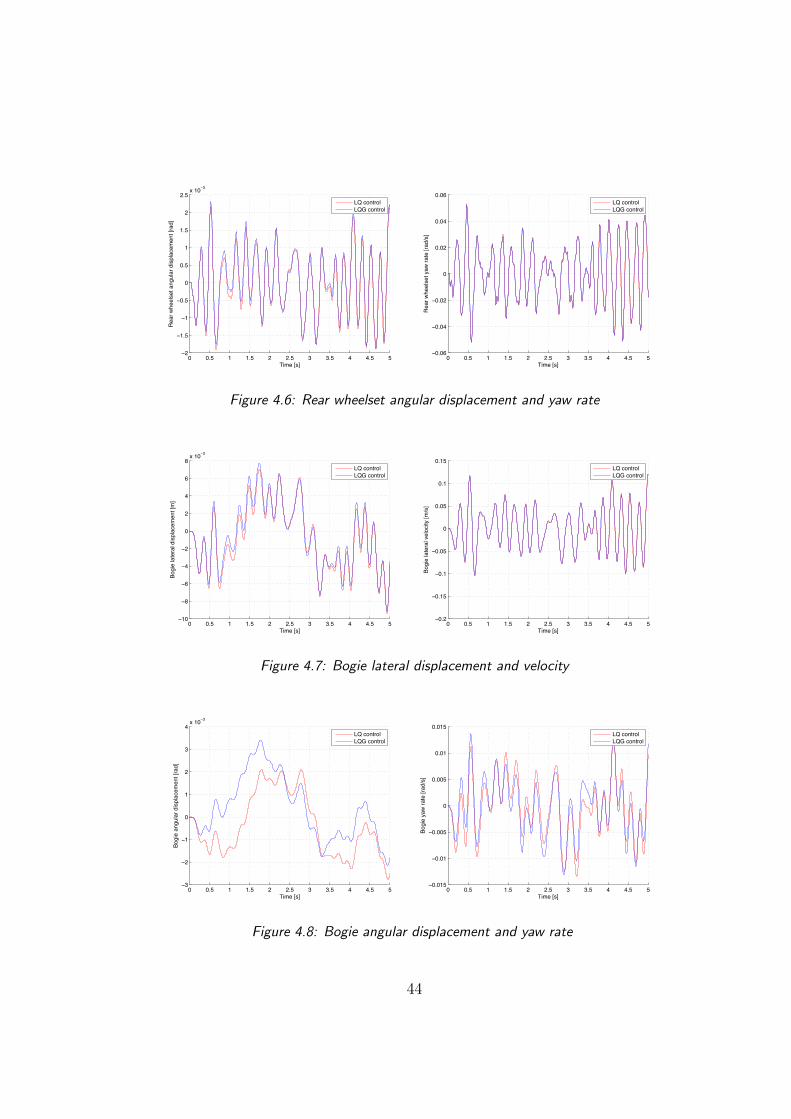
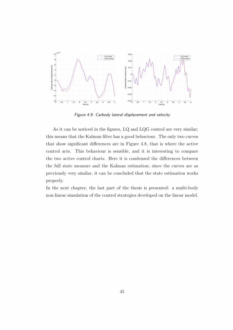
As it can be noticed in the figures, LQ and LQG control are very similar;
this means that the Kalman filter has a good behaviour. The only two curves
that show significant differences are in Figure 4.8, that is where the active
control acts. This behaviour is sensible, and it is interesting to compare
the two active control charts. Here it is condensed the differences between
the full state measure and the Kalman estimation; since the curves are as
previously very similar, it can be concluded that the state estimation works
properly.
In the next chapter, the last part of the thesis is presented: a multi-body
non-linear simulation of the control strategies developed on the linear model.
45
Chapter 5
Control strategy simulation
with a multi-body non-linear
model
5.1 Introduction
After having developed and tuned the control strategies on the linear model,
the results are compared with a non-linear multi-body simulation. In this
Chapter, only the LQ control strategy has been implemented, because of
the long implementation of a state estimator in the multi-body simulator
and the lack of time due to time constraints. It has been decided to assess
the results with a more complicated and complete type of simulation mainly
because the aim of the thesis can be validated only on a curved track. With
a linear model is very difficult to represent the real dynamics of a curved
track, because of several limitations:
• linear modellization of wheel rail contact mechanism
• complex curved track equation of motion writing
• non reliable results, due to the large semplification of the vehicle dy-
namics
46
Therefore, a non-linear multi-body simulation has been chosen because it
better describes the reality. At Politecnico di Milano some multi-body models
have been developed and used in past research programmes, hence in this
work one of these models has been used to describe the vehicle studied in the
linear model. In particular, the simulator taken into account is described in
[10]. The multi-body model contains:
• a carbody, modelled as a single rigid body
• a bogie assembly, modelled as a rigid bogie frame connected by primary
suspensions to two exible wheelsets
• other bodies attached either to a carbody or to a bogie frame (e.g.
motors, converters etc.), modelled as rigid
These elementary units are connected to each other by elastic and damp-
ing elements (linear and nonlinear) reproducing the secondary suspensions
and other elastic connections such as links between carbodies, elastic motor
suspension etc. By combining the above listed elementary units, any specic
trainset architecture may be derived; in the case studied in this work, a rail-
way vehicle formed by two bogies and one carbody has been set up.
Each rigid body is assigned with five degrees of freedom, the forward speed
of body centre of mass being set to a constant value V , whereas for each
flexible wheelset, the movement with respect to the moving reference is dened
as the linear combination of the unconstrained wheelset eigenmodes.
Besides the multi-body model construction, the other important parameter is
the wheel-rail contact modellization. Both contact path geometry and creep
coefficient have been considered as non linear. These assumptions imply a
very different model of wheel-rail contact from the one used in the linear
model described in Chapter 2. Therefore, a direct comparison of a time his-
tory between the linear and the non linear model would not be meaningful.
For example, in Figure 5.1 the blue line represents the multi body simula-
tion, the green line the linear simulation. The simulation characteristics are
v = 40 m/s, λ = 0.025. As it can be seen, the two lines follow the same
47
0.5 1 1.5 2 2.5 3 3.5 4 4.5
−8
−6
−4
−2
0
2
4
6
8
10
12x 10−3
Time [s]
Car
body
late
ral d
ispl
acem
ent [
m]
lateral carbody disp
Multi−body modelLinear model
0.5 1 1.5 2 2.5 3 3.5 4 4.5
−0.025
−0.02
−0.015
−0.01
−0.005
0
0.005
0.01
0.015
0.02
0.025
Time [s]
Car
body
late
ral v
eloc
ity [m
/s]
lateral carbody vel
Multi−body modelLinear model
Figure 5.1: Carbody lateral displacement and velocity - comparison of linear and non-
linear simulation for the passive vehicle
trend, but they are not very close. Therefore, multi-body simulation results
will be compared only among themselves, hence will be compared the pass-
ive model, the passive model with the lowered primary yaw stiffnes, and the
active model.
5.2 Simulation scenarios
In order to assess the performances of the system and to display the results,
a number of different running situations have been simulated.
On straght track, the multi-body simulation has been performed with lat-
eral track irregulaties, as done for the linear model. The vehicle speed is
v = 40m/s.
Concerning to the curving situation, the simulations have been done without
disturbances, in order to display better the behaviour of the system and
then to make the comparisons easier. The simulation characteristics are
v = 31.5m/s, curve radius R = 500m, non compensated lateral acceleration
a = 1m/s2, track cant h = 150mm.
48
For both the track situations, the configurations taken into account are:
• passive system
• passive system with lowered value of primary yaw stiffness
• active system
5.3 Simulation results
In this section the final results are displayed, focusing the attention on the
curving performances related to the primary yaw stiffness.
5.3.1 Straight track results
In order to assess the straight track performances, a comparison on several
stability indices has been done. The European norm EN14363 defines the
boundaries in which the railway vehicle must be; in particular, one of those
boundaries regards the maximum lateral acceleration of each wheelset. This
information can be assumed as the safety limit for stability condition. This
measure must be done with an accelerometer put on the axlebox of the wheel-
set.
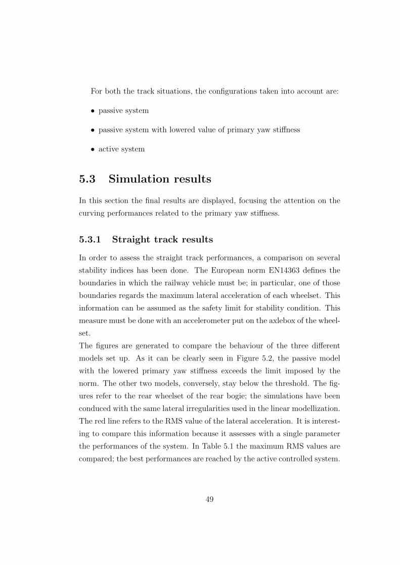
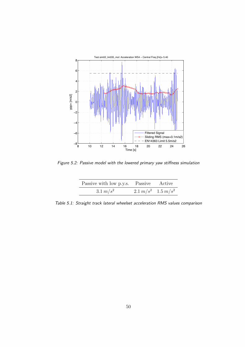
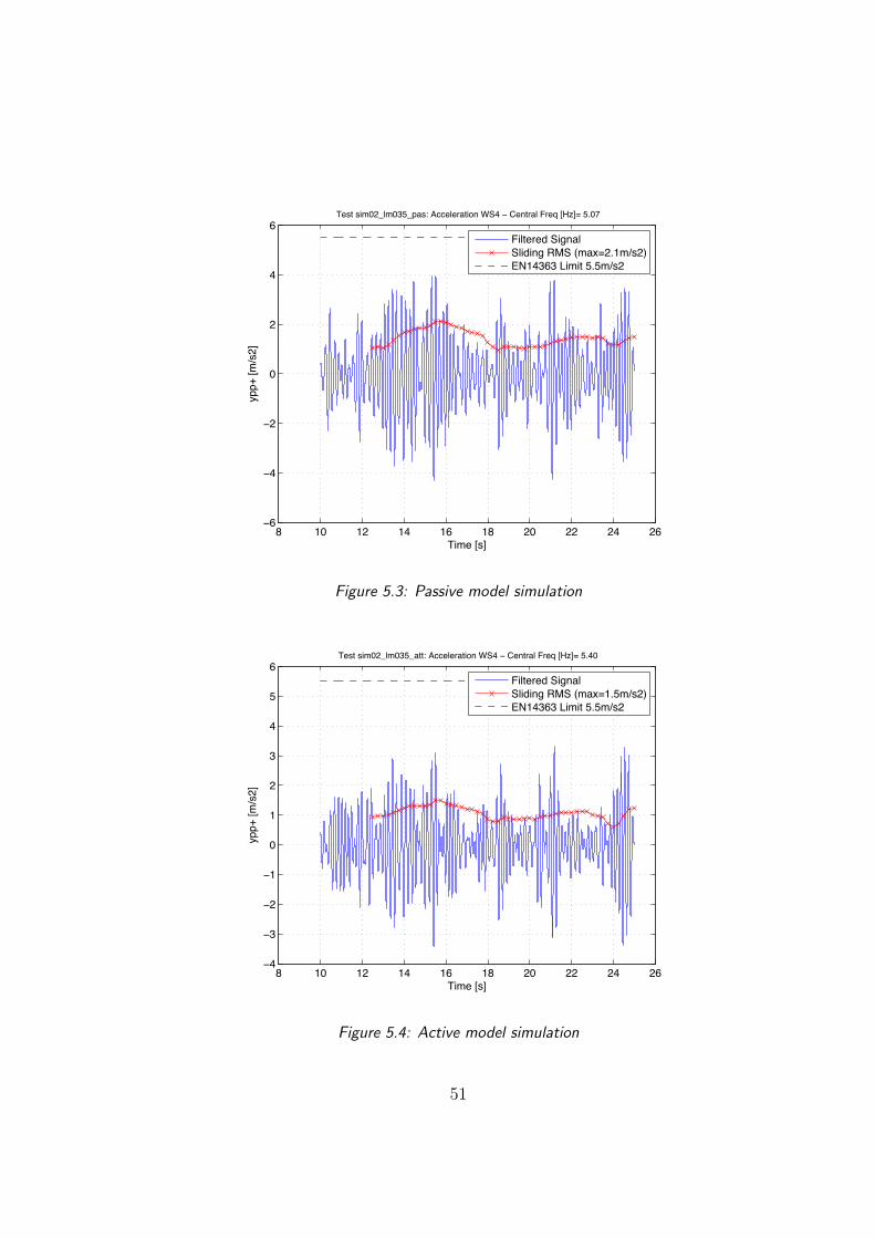
The figures are generated to compare the behaviour of the three different
models set up. As it can be clearly seen in Figure 5.2, the passive model
with the lowered primary yaw stiffness exceeds the limit imposed by the
norm. The other two models, conversely, stay below the threshold. The fig-
ures refer to the rear wheelset of the rear bogie; the simulations have been
conduced with the same lateral irregularities used in the linear modellization.
The red line refers to the RMS value of the lateral acceleration. It is interest-
ing to compare this information because it assesses with a single parameter
the performances of the system. In Table 5.1 the maximum RMS values are
compared; the best performances are reached by the active controlled system.
49
8 10 12 14 16 18 20 22 24 26−8
−6
−4
−2
0
2
4
6
8Test sim02_lm035_mol: Acceleration WS4 − Central Freq [Hz]= 5.40
Time [s]
ypp+
[m/s
2]
Filtered SignalSliding RMS (max=3.1m/s2)EN14363 Limit 5.5m/s2
Figure 5.2: Passive model with the lowered primary yaw stiffness simulation
Passive with low p.y.s. Passive Active
3.1m/s2 2.1m/s2 1.5m/s2
Table 5.1: Straight track lateral wheelset acceleration RMS values comparison
50
8 10 12 14 16 18 20 22 24 26−6
−4
−2
0
2
4
6Test sim02_lm035_pas: Acceleration WS4 − Central Freq [Hz]= 5.07
Time [s]
ypp+
[m/s
2]
Filtered SignalSliding RMS (max=2.1m/s2)EN14363 Limit 5.5m/s2
Figure 5.3: Passive model simulation
8 10 12 14 16 18 20 22 24 26−4
−3
−2
−1
0
1
2
3
4
5
6Test sim02_lm035_att: Acceleration WS4 − Central Freq [Hz]= 5.40
Time [s]
ypp+
[m/s
2]
Filtered SignalSliding RMS (max=1.5m/s2)EN14363 Limit 5.5m/s2
Figure 5.4: Active model simulation
51
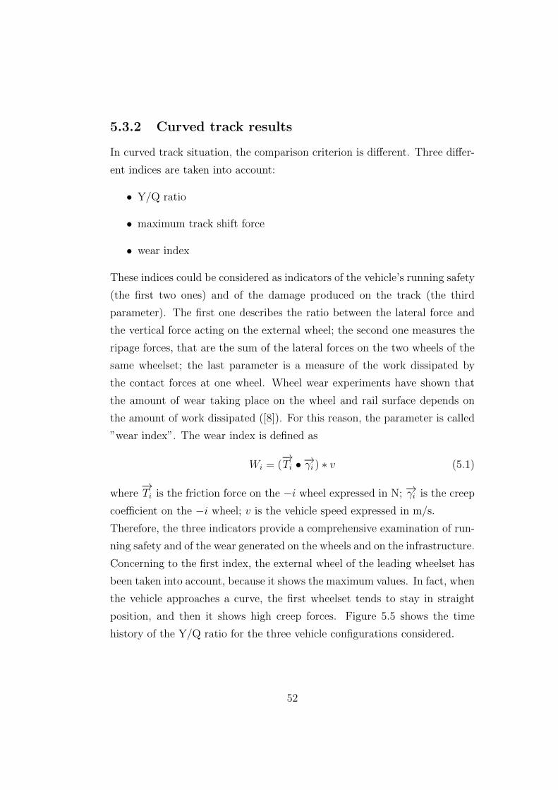
5.3.2 Curved track results
In curved track situation, the comparison criterion is different. Three differ-
ent indices are taken into account:
• Y/Q ratio
• maximum track shift force
• wear index
These indices could be considered as indicators of the vehicle’s running safety
(the first two ones) and of the damage produced on the track (the third
parameter). The first one describes the ratio between the lateral force and
the vertical force acting on the external wheel; the second one measures the
ripage forces, that are the sum of the lateral forces on the two wheels of the
same wheelset; the last parameter is a measure of the work dissipated by
the contact forces at one wheel. Wheel wear experiments have shown that
the amount of wear taking place on the wheel and rail surface depends on
the amount of work dissipated ([8]). For this reason, the parameter is called
”wear index”. The wear index is defined as
Wi = (−→Ti • −→γi ) ∗ v (5.1)
where−→Ti is the friction force on the −i wheel expressed in N; −→γi is the creep
coefficient on the −i wheel; v is the vehicle speed expressed in m/s.
Therefore, the three indicators provide a comprehensive examination of run-
ning safety and of the wear generated on the wheels and on the infrastructure.
Concerning to the first index, the external wheel of the leading wheelset has
been taken into account, because it shows the maximum values. In fact, when
the vehicle approaches a curve, the first wheelset tends to stay in straight
position, and then it shows high creep forces. Figure 5.5 shows the time
history of the Y/Q ratio for the three vehicle configurations considered.
52
0 5 10 15 20 25 30−0.3
−0.25
−0.2
−0.15
−0.1
−0.05
0
0.05
Time [s]
Y/Q
Rat
io
Y/Q Ratio comparison
Passive systemPassive system with soft p.y.sActive system
Figure 5.5: Y/Q Ratio comparison
It is observed that in the passive model, as expected, the Y/Q ratio is
bigger than the other two models. Moreover, it is remarkable that the active
model and the passive with the lowered primary yaw stiffness have the same
behaviour, with slight differences. This is due to the fact that the simulation
speed is much lower than the critical speed, hence the action of the active
control is small.
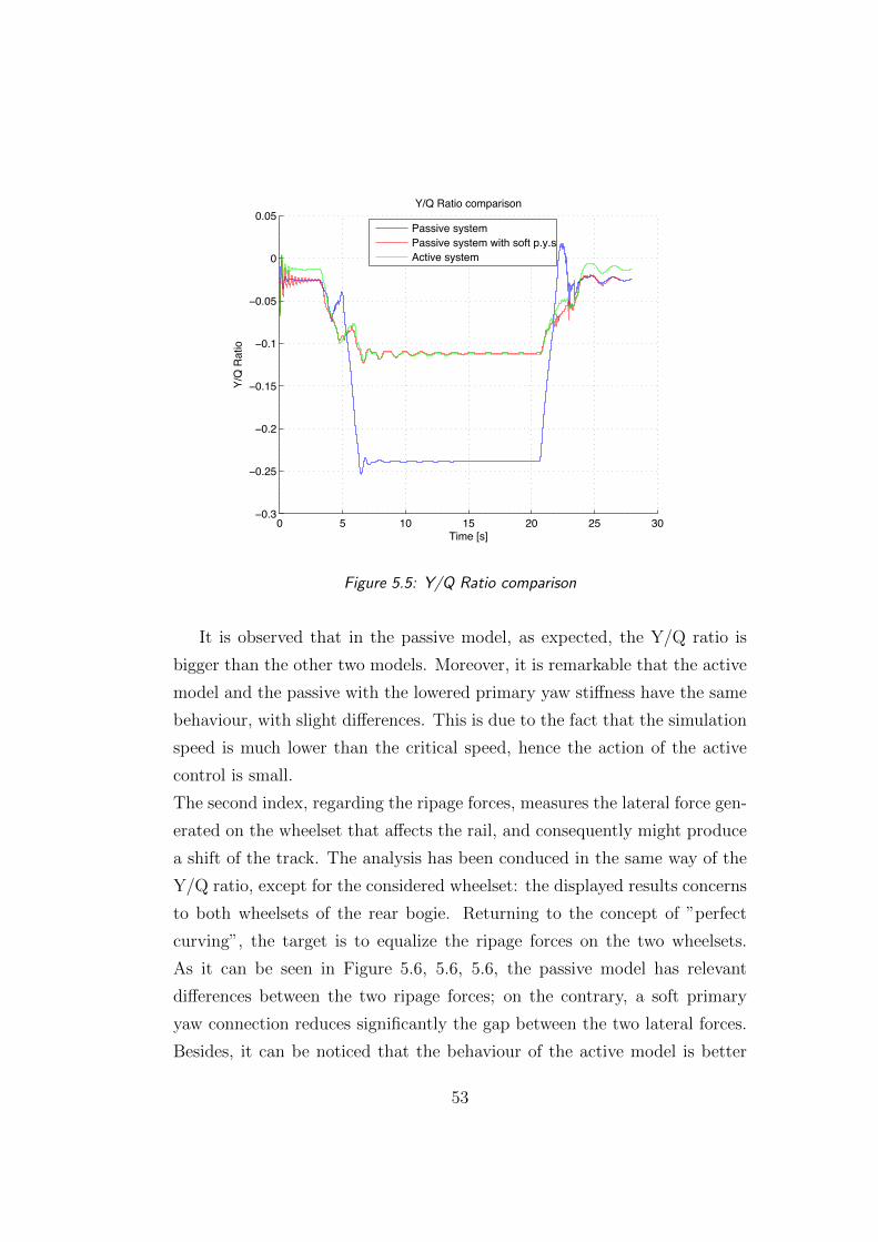
The second index, regarding the ripage forces, measures the lateral force gen-
erated on the wheelset that affects the rail, and consequently might produce
a shift of the track. The analysis has been conduced in the same way of the
Y/Q ratio, except for the considered wheelset: the displayed results concerns
to both wheelsets of the rear bogie. Returning to the concept of ”perfect
curving”, the target is to equalize the ripage forces on the two wheelsets.
As it can be seen in Figure 5.6, 5.6, 5.6, the passive model has relevant
differences between the two ripage forces; on the contrary, a soft primary
yaw connection reduces significantly the gap between the two lateral forces.
Besides, it can be noticed that the behaviour of the active model is better
53

0 5 10 15 20 25 30−20000
−15000
−10000
−5000
0
5000
Time [s]
ripag
e fo
rces
[N]
Passive system ripage forces
Fourth wheelsetThird wheelset
Figure 5.6: Passive model ripage forces
than the passive with the lower primary yaw stiffness; in particular, it has
got reduced vibrations and more equalized ripage forces. In this case the
control action works reducing the vibrations and steering the bogie towards
the inside of the curve. In fact, when the vehicle is running on a curve, the
bogie tents to stay in a understeer position, due to the dynamics of the sys-
tem. Active control, in order to equalize the ripage forces, steers the bogie,
obtaining a better result compared to the others.
Concerning to the wear index, the results are displayed as the power dis-
sipation on each wheelset caused by the longitudinal and trasversal creep
forces. Then the dissipated energy is displayed, computed as the integral of
the power dissipation. The numerical results are summarized in Table 5.2,
where the total dissipated energy on each wheel is listed; trasversal and lon-
gitudinal components have been summed. In the figures, the trailing wheelset
of the rear bogie wheelset has been taken into account. As it can be clearly
seen (Table 5.2), a drastic reduction of energy dissipation can be obtained
using a soft primary yaw stiffness connection. Moreover, as seen for the ri-
54
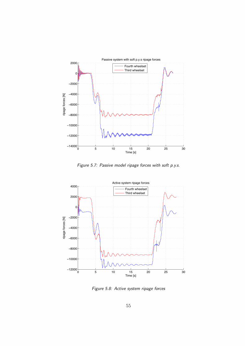
0 5 10 15 20 25 30−14000
−12000
−10000
−8000
−6000
−4000
−2000
0
2000
Time [s]
ripag
e fo
rces
[N]
Passive system with soft p.y.s ripage forces
Fourth wheelsetThird wheelset
Figure 5.7: Passive model ripage forces with soft p.y.s.
0 5 10 15 20 25 30−12000
−10000
−8000
−6000
−4000
−2000
0
2000
4000
Time [s]
ripag
e fo
rces
[N]
Active system ripage forces
Fourth wheelsetThird wheelset
Figure 5.8: Active system ripage forces
55
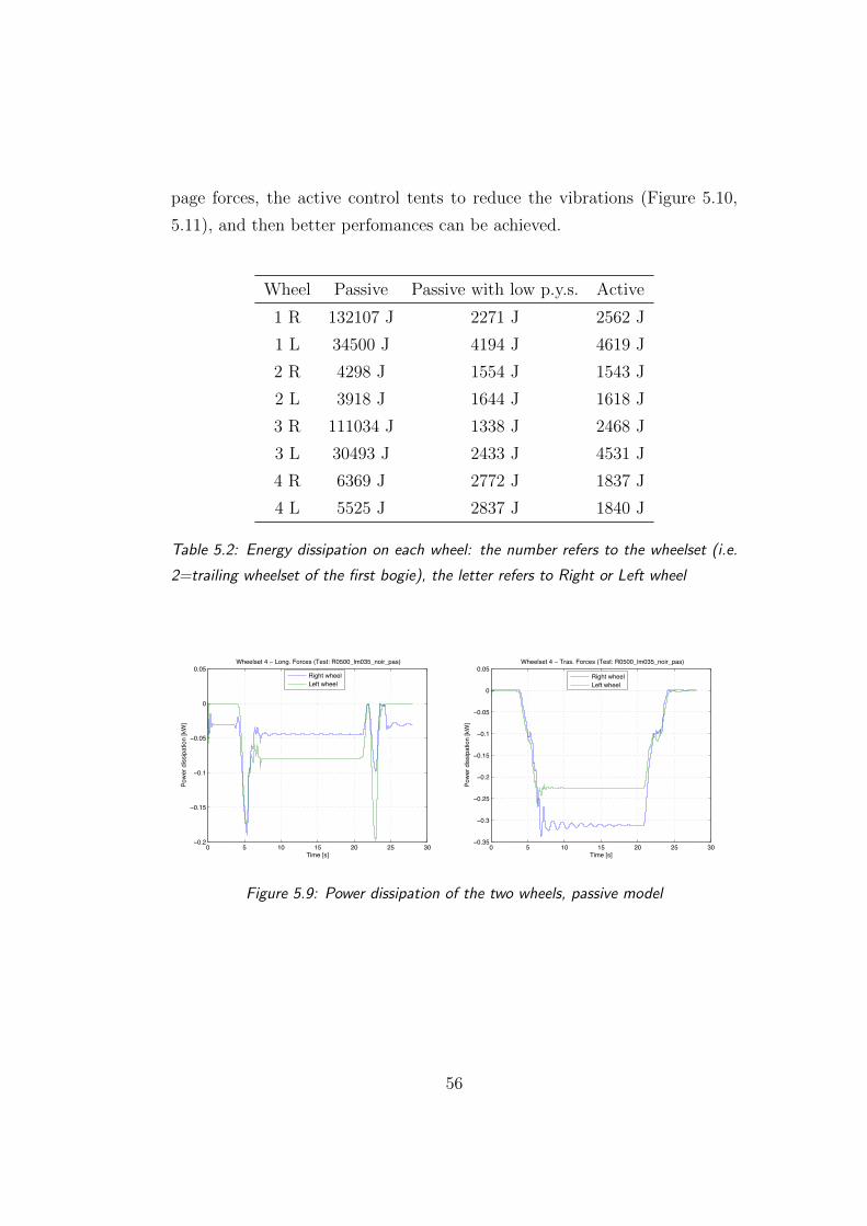
page forces, the active control tents to reduce the vibrations (Figure 5.10,
5.11), and then better perfomances can be achieved.
Wheel Passive Passive with low p.y.s. Active
1 R 132107 J 2271 J 2562 J
1 L 34500 J 4194 J 4619 J
2 R 4298 J 1554 J 1543 J
2 L 3918 J 1644 J 1618 J
3 R 111034 J 1338 J 2468 J
3 L 30493 J 2433 J 4531 J
4 R 6369 J 2772 J 1837 J
4 L 5525 J 2837 J 1840 J
Table 5.2: Energy dissipation on each wheel: the number refers to the wheelset (i.e.
2=trailing wheelset of the first bogie), the letter refers to Right or Left wheel
0 5 10 15 20 25 30−0.2
−0.15
−0.1
−0.05
0
0.05Wheelset 4 − Long. Forces (Test: R0500_lm035_noir_pas)
Time [s]
Pow
er d
issi
patio
n [k
W]
Right wheelLeft wheel
0 5 10 15 20 25 30−0.35
−0.3
−0.25
−0.2
−0.15
−0.1
−0.05
0
0.05Wheelset 4 − Tras. Forces (Test: R0500_lm035_noir_pas)
Time [s]
Pow
er d
issi
patio
n [k
W]
Right wheelLeft wheel
Figure 5.9: Power dissipation of the two wheels, passive model
56

0 5 10 15 20 25 30−0.09
−0.08
−0.07
−0.06
−0.05
−0.04
−0.03
−0.02
−0.01
0
0.01Wheelset 4 − Long. Forces (Test: R0500_lm035_noir_mol)
Time [s]
Pow
er d
issi
patio
n [k
W]
Right wheelLeft wheel
0 5 10 15 20 25 30−0.16
−0.14
−0.12
−0.1
−0.08
−0.06
−0.04
−0.02
0
0.02Wheelset 4 − Tras. Forces (Test: R0500_lm035_noir_mol)
Time [s]
Pow
er d
issi
patio
n [k
W]
Right wheelLeft wheel
Figure 5.10: Power dissipation of the two wheels, passive model with soft p.y.s.
0 5 10 15 20 25 30−0.07
−0.06
−0.05
−0.04
−0.03
−0.02
−0.01
0
0.01Wheelset 4 − Long. Forces (Test: R0500_lm035_noir_att)
Time [s]
Pow
er d
issi
patio
n [k
W]
Right wheelLeft wheel
0 5 10 15 20 25 30−0.09
−0.08
−0.07
−0.06
−0.05
−0.04
−0.03
−0.02
−0.01
0
0.01Wheelset 4 − Tras. Forces (Test: R0500_lm035_noir_att)
Time [s]
Pow
er d
issi
patio
n [k
W]
Right wheelLeft wheel
Figure 5.11: Power dissipation of the two wheels, active model
5.4 Multi-body simulations conclusions
In this Chapter a multi-body non-linear simulator has been used in order
to test the performances of the different railway vehicle models taken into
account in this thesis.
Firstly, a straight track test has been done in order to check the behaviour of
the models on the multi-body simulator. Then, established the sensibleness
of the results, some tests on curved track have been conduced. In particular,
in order to assess the curving performances, three indices have been used:
Y/Q ratio, track shift force and the wear index. With these three indices
it was possible to validate the advatages of an active control applied on a
57

vehicle with soft primary yaw stiffness connection. The initial hypotesis of
better curving performances have been verified and quantified by the test
performed on the different models in different situations.
58
Chapter 6
Conclusions
In this study the potential improvements in curving performance through
the use of a secondary yaw control has been presented. Curving performaces
have been improved through a reduction of the primary yaw stiffness. Act-
ive control provides the needed stabilization, where a passive damper cannot
give stability. The improved curving means less wear on the wheels and rails,
and therefore lower maintenance costs. It also improves the running safety
in a curve.
A linear half vehicle plan view has been developed in order to study the prop-
erties of the mechanical system, and to allow a control strategy development.
Basically, two different types of inputs have been used, a lateral step input
and a measured lateral track disturbance. Two different control strategies
have been developed, an LQ full state control and an LQG control with state
estimation. A sensing assessment has been done in order to describe the
mechanical system equipped with the sensors.
The performances of the three different models (passive, LQ, LQG) have
been firstly compared on the linear model, and then with a more precise
multi-body non-linear simulator, which provides accurate results also for the
curving condition. The simulations have been conduced both in straight and
curved track, highlighting in every situation the advantages of an active con-
trol utilization.
59

Further reaserch, starting from this work, could be identified as:
• development of a different control strategy, for example an H∞ ap-
proach
• a modellization of the actuator, in order to study the dynamic influence
on the system
60
Bibliography
[1] Wickens A.H. Fundamentals of rail vehicle dynamics: guidance and
stability. Swets and Zeitlinger Publisher, 2003.
[2] Bruni S Braghin F. and Resta F. Active yaw damper for the improve-
ment of railway vehicle stability and curving performances: simulations
and experimental results. Vehicle System Dynamics Vol. 44, No. 11,
November 2006, 857-869, 2006.
[3] Mei T.X. Bruni S., Goodall R.M. and H. Tsunashima. Control and
monitoring for railway vehicle dynamics. Vehicle System Dynamics:
International Journal of Vehicle Mechanics and Mobility, vol.45(7-8),
Special Issue: State of the Art Papers of the 20th IAVSD Symposium,
pp 743-779, 2007.
[4] Diana G. and Cheli F. Dinamica e vibrazioni dei sistemi meccanici.
UTET Libreria, 1993.
[5] Mirzapour M. Hubbard P., Mei T.X. and Ward C. Half cost trains:
design for control. Rail Research Association UK, 2013.
[6] Suda Y. Michitsuji Y. Tanimoto M. Miyauchi E. Matsumoto A. Ohno H.,
Mizuma T. and Sato Y. Research on high curving performance
trucksconcept and basic characteristics of active-bogie-steering-truck.
Vehicle System Dynamics, 41(suppl), 3342, 2004.
[7] Goodall R.M. Persson R. and K. Sasaki. Carbody tilting - technologies
and benefits. Vehicle System Dynamics, 47(8), pp. 949-981, 2009.
61

[8] Lewis R. and Olofsson U. Wheel-rail interface handbook. Woodhead
Publishing, 2009.
[9] Goodall R.M. and Mei T.X. Kalman filters applied to actively controlled
railway vehicle suspensions. Transaction of the Institute of Measurement
and Control, Vol. 23, No 3, 163-181, 2001.
[10] Alfi S. and Bruni S. Mathematical modelling of trainturnout interaction.
Vehicle System Dynamics: International Journal of Vehicle Mechanics
and Mobility, 47:5, 551-574, 2009.
62
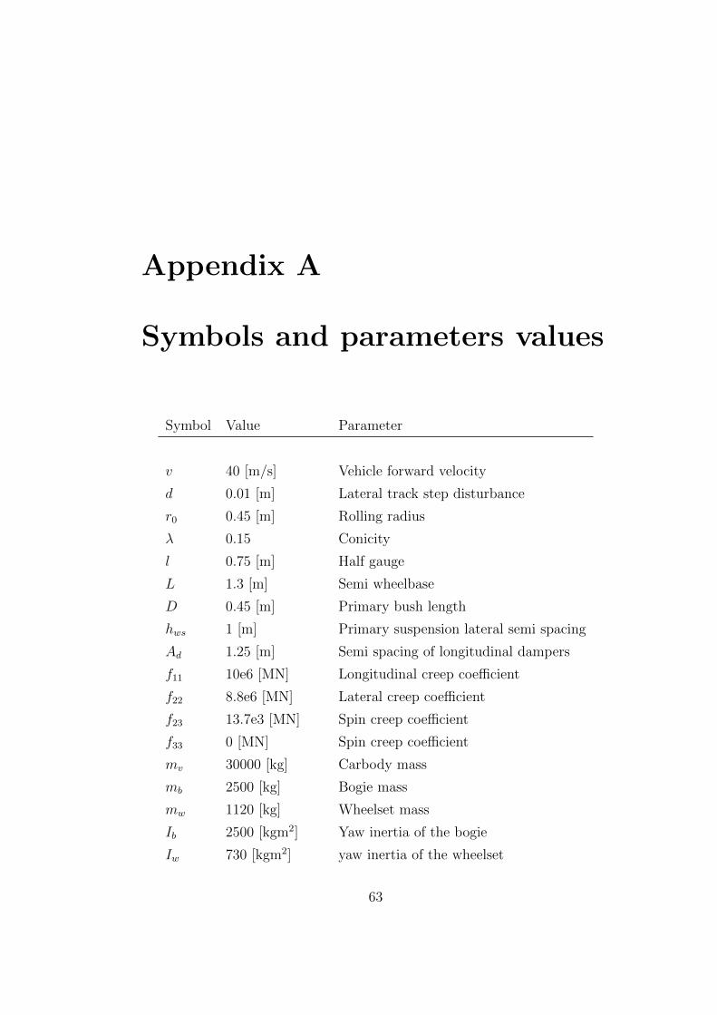
Appendix A
Symbols and parameters values
Symbol Value Parameter
v 40 [m/s] Vehicle forward velocity
d 0.01 [m] Lateral track step disturbance
r0 0.45 [m] Rolling radius
λ 0.15 Conicity
l 0.75 [m] Half gauge
L 1.3 [m] Semi wheelbase
D 0.45 [m] Primary bush length
hws 1 [m] Primary suspension lateral semi spacing
Ad 1.25 [m] Semi spacing of longitudinal dampers
f11 10e6 [MN] Longitudinal creep coefficient
f22 8.8e6 [MN] Lateral creep coefficient
f23 13.7e3 [MN] Spin creep coefficient
f33 0 [MN] Spin creep coefficient
mv 30000 [kg] Carbody mass
mb 2500 [kg] Bogie mass
mw 1120 [kg] Wheelset mass
Ib 2500 [kgm2] Yaw inertia of the bogie
Iw 730 [kgm2] yaw inertia of the wheelset
63
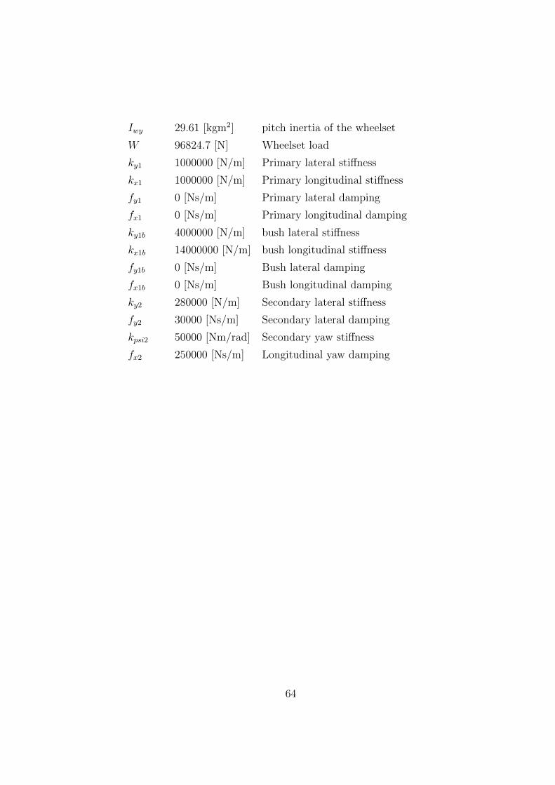
Iwy 29.61 [kgm2] pitch inertia of the wheelset
W 96824.7 [N] Wheelset load
ky1 1000000 [N/m] Primary lateral stiffness
kx1 1000000 [N/m] Primary longitudinal stiffness
fy1 0 [Ns/m] Primary lateral damping
fx1 0 [Ns/m] Primary longitudinal damping
ky1b 4000000 [N/m] bush lateral stiffness
kx1b 14000000 [N/m] bush longitudinal stiffness
fy1b 0 [Ns/m] Bush lateral damping
fx1b 0 [Ns/m] Bush longitudinal damping
ky2 280000 [N/m] Secondary lateral stiffness
fy2 30000 [Ns/m] Secondary lateral damping
kpsi2 50000 [Nm/rad] Secondary yaw stiffness
fx2 250000 [Ns/m] Longitudinal yaw damping
64