rapid city, south dakota depreciation study...
TRANSCRIPT

BLACK HiLLS POV'VER
Rapid City, South Dakota
DEPRECIATION STUDY
CALCULATED ANNUAL DEPRECIATION ACCRUALS
RELATED TO ELECTRIC PLANT
AS OF DECEMBER 31, 2012
GANNETT FLEMING, INC. - VALUATION AND RATE DIVISION
Harrisburg, Pennsylvania
EXHIBIT JJS-2 (Abbreviated)

ii
~ 6annettF/eming Exceiience Deiivered As Promised
Black Hills Power 625 Ninth Street Rapid City, SD 57701
Attention Mr. Chris Kilpatrick Director of Rates
Ladies and Gentlemen:
November 27, 2013
Pursuant to your request, we have conducted a depreciation study related to the electric plant of Black Hills Power. The study results include annual depreciation rates as of December 31, 2012. The attached report presents a description of the methods used in the estimation of depreciation, summaries of annual and accrued depreciation, the statistical support for the life and net salvage estimates and the detailed tabulations of annual and accrued depreciation.
JJS/krm
057073
Respectfu!!y submitted,
GANNETT FLEMING, INC.
JOHN J. SPANOS Sr. Vice President Valuation and Rate Division
Gannett Fleming, Inc. Valuation and Rate Division
P.O. Box 67100 •Harrisburg, PA 17106-7100 • 207 Senate Avenue• Camp HHJ, PA 17011-2316 t: 717.763.7211·f:717.763.4590
www.gannettfleming.com • www.gfvrd.com
,o'"··.,,

\ I CONTENTS
PART I. INTRODUCTION
Scope . . . . . . . . . . . . . . . . . . . . . . . . . . . . . . . . . . . . . . . . . . . . . . . . . . . . . . . . . 1-2 Plan of Report . . . . . . . . . . . . . . . . . . . . . . . . . . . . . . . . . . . . . . . . . . . . . . . . . . . 1-2 Basis of Study . . . . . . . . . . . . . . . . . . . . . . . . . . . . . . . . . . . . . . . . . . . . . . . . . . . 1-3
Depreciation . . . . . . . . . . . . . . . . . . . . . . . . . . . . . . . . . . . . . . . . . . . . . . . . 1-3 Service Life Estimates . . . . . . . . . . . . . . . . . . . . . . . . . . . . . . . . . . . . . . . . 1-3 Net Salvage Estimates . . . . . . . . . . . . . . . . . . . . . . . . . . . . . . . . . . . . . . . . 1-4
PART 11. METHODS USED IN THE ESTIMATION OF DEPRECIATION
Depreciation . . . . . . . . . . . . . . . . . . . . . . . . . . . . . . . . . . . . . . . . . . . . . . . . . . . . 11-2 Service Life and Net Salvage Estimation . . . . . . . . . . . . . . . . . . . . . . . . . . . . . . 11-2
Average Service Life . . . . . . . . . . . . . . . . . . . . . . . . . . . . . . . . . . . . . . . . . 11-2 Survivor Curves . . . . . . . . . . . . . . . . . . . . . . . . . . . . . . . . . . . . . . . . . . . . . 11-3
Iowa Type Curves . . . . . . . . . . . . . . . . . . . . . . . . . . . . . . . . . . . . . . . . . 11-3 Retirement Rate Method of Analysis . . . . . . . . . . . . . . . . . . . . . . . . . . . . . 11-10
Schedules of Annual Transactions in Plant Records . . . . . . . . . . . . . . 11-11 Schedule of Plant Exposed to Retirement . . . . . . . . . . . . . . . . . . . . . . 11-14 Original Life Table . . . . . . . . . . . . . . . . . . . . . . . . . . . . . . . . . . . . . . . . . 11-16 Smoothing the Original Survivor Curve . . . . . . . . . . . . . . . . . . . . . . . . . 11-18
Service Life Considerations . . . . . . . . . . . . . . . . . . . . . . . . . . . . . . . . . . . . 11-23 Salvage Analysis . . . . . . . . . . . . . . . . . . . . . . . . . . . . . . . . . . . . . . . . . . . . 11-26 Net Salvage Considerations . . . . . . . . . . . . . . . . . . . . . . . . . . . . . . . . . . . . 11-26
Calculation of Annual and Accrued Depreciation . . . . . . . . . . . . . . . . . . . . . . . . 11-28 Single Unit of Property . . . . . . . . . . . . . . . . . . . . . . . . . . . . . . . . . . . . . . . . 11-29 Group Depreciation Procedures . . . . . . . . . . . . . . . . . . . . . . . . . . . . . . . . . 11-29
Remaining Life Annual Accruals . . . . . . . . . . . . . . . . . . . . . . . . . . . . . . 11-30 Average Service Life Procedure . . . . . . . . . . . . . . . . . . . . . . . . . . . . . . 11-30
Calculation of Annual and Accrued Amortization . . . . . . . . . . . . . . . . . . . . . . . . 11-31
- iii -

CONTE~~TS, cont.
PART Ill. RESULTS OF STUDY
Qualification of Results .......................................... . Description of Statistical Support .................................. . Description of Depreciation Tabulations ............................. . Summary of Estimated Survivor Curves, Net Salvage, Original Cost,
Book Depreciation Reserve and Calculated Annual Depreciation Accrual Rates as of December 31, 2012 .......................... .
Service Life Statistics ........................................... . Net Salvage Statistics ........................................... . Depreciation Calculations ........................................ .
- iv -
111-2 111-3 111-3
111-4 111-9
111-118 111-149

)
1-1 PART I. INTRODUCTION

BLACK HILLS PO\lVER
DEPRECIATION STUDY
PART I. INTRODUCTION
SCOPE
This report presents the results of the depreciation study prepared for Black Hills
Power (the Company) as applied to electric plant in service as of December 31, 2012. The
report relates to the concepts, methods and basic judgments which underlie recommended
annual depreciation accrual rates and amounts related to current electric plant in service.
The service life and net salvage estimates resulting from the study were based on
informed judgment which incorporated analyses of historical plant retirement data as
recorded through 2012; a review of Company practice and outlook as they relate to plant
operation and retirement; and consideration of current practice in the electric industry,
including knowledge of service life and salvage estimates used for other electric properties.
PLAt" OF REPORT
Part I, Introduction, includes brief statements of the scope and basis of the study.
Part II presents descriptions of the methods used in the service life and net salvage studies
and the methods and procedures used in the calculation of depreciation. Part Ill presents
the results of the study, including a summary table, survivor curve charts and life tables
resulting from the retirement rate method of analysis, tabular results of the historical net
salvage analyses, and detailed tabulations of the calculated remaining lives and annual
accruals.
1-2
) BASIS OF STUDY
Depreciation
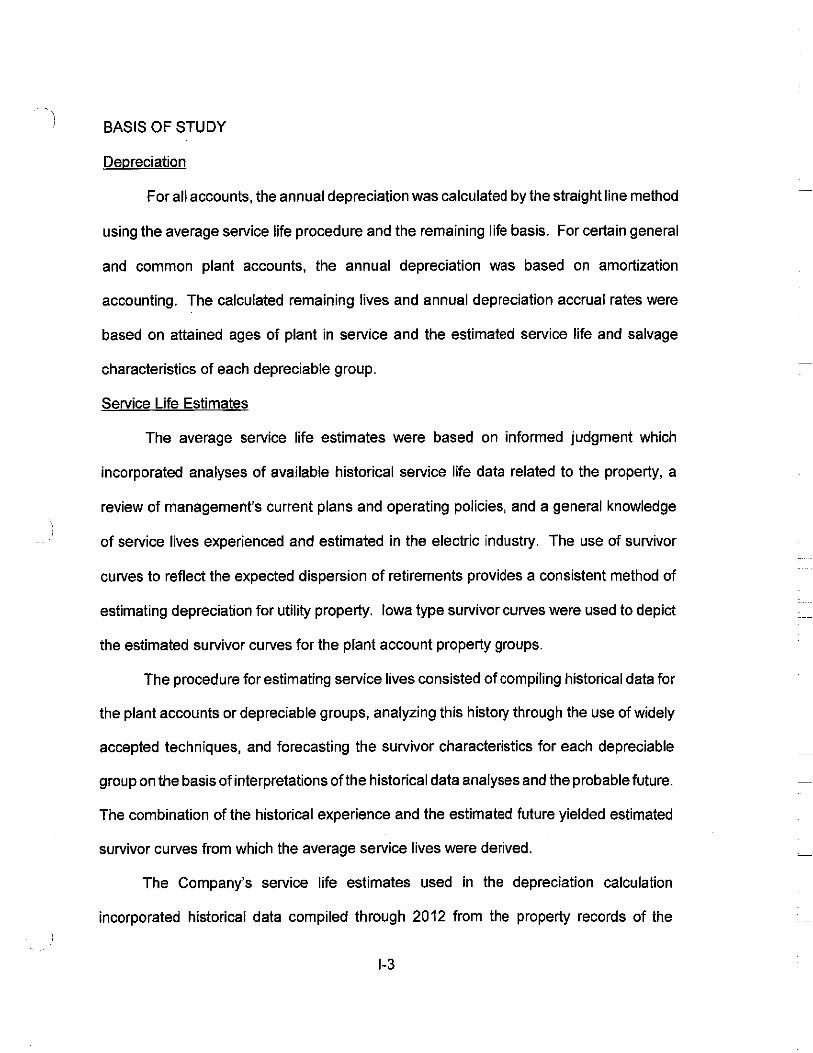
For all accounts, the annual depreciation was calculated by the straight line method
using the average service life procedure and the remaining life basis. For certain general
and common plant accounts, the annual depreciation was based on amortization
accounting. The calculated remaining lives and annual depreciation accrual rates were
based on attained ages of plant in service and the estimated service life and salvage
characteristics of each depreciable group.
Service Life Estimates
The average service life estimates were based on informed judgment which
incorporated analyses of available historical service life data related to the property, a
review of management's current plans and operating policies, and a general knowledge
of service lives experienced and estimated in the electric industry. The use of survivor
curves to reflect the expected dispersion of retirements provides a consistent method of
estimating depreciation for utility property. Iowa type survivor curves were used to depict
the estimated survivor curves for the plant account property groups.
The procedure for estimating service lives consisted of compiling historical data for
the plant accounts or depreciable groups, analyzing this history through the use of widely
accepted techniques, and forecasting the survivor characteristics for each depreciable
group on the basis of interpretations of the historical data analyses and the probable future.
The combination of the historical experience and the estimated future yielded estimated
survivor curves from which the average service lives were derived.
The Company's service life estimates used in the depreciation calculation
incorporated historical data compiled through 2012 from the property records of the
1-3

Company. Such data included p!ant additions, retirements, transfers and other activity.
Generally, retirement data for the years 1950 through 2012 were used in the actuarial life
table computations which were the primary statistical support of the service life estimates.
A general understanding of the function of the plant and information with respect to
the reasons for past retirements and the expected future causes of retirement was
obtained through discussions with operating and management personnel conducted during
the course of the service life study. Information regarding plans for the future was
incorporated in the interpretation and extrapolation of the statistical analyses.
Net Salvage Estimates
The estimates of net salvage were based in part on histor.ical data compiled for the
years 1997 through 2012. Gross salvage and cost of removal as recorded to the
depreciation reserve account and related to experienced retirements were used.
Percentages of the cost of plant retired were calculated for each component of net salvage,
on both annual and three-year moving average bases. The most recent five-year average
also was calculated for consideration. The estimates of net salvage are expressed as
percentages of the cost of plant retired.
1-4

11-1 PART 11. METHODS USED IN
THE ESTIMATION OF DEPRECIATION

DEPRECIATION
PART II. METHODS USED IN THE ESTiMATiON OF DEPRECIATION
Depreciation, in public utility regulation, is the loss in service value not restored by
current repairs or covered by insurance.
Depreciation, as used in accounting, is a method of distributing fixed capital costs,
less net salvage, over a period of time by allocating annual amounts to expense. Each
annual amount of such depreciation expense is part of that year's total cost of providing
utility service. Normally, the period of time over which the fixed capital cost is allocated to
the cost of service is equal to the period of time over which an item renders service, that
is, the item's service life. The most prevalent method of allocation is to distribute an equal
amount of cost to each year of service life. This method is known as the straight line
method of depreciation.
The calculation of annual depreciation based on the straight line method requires
the estimation of average life and net salvage. These subjects are discussed in the
sections which follow.
SERVICE LIFE AND NET SALVAGE ESTIMATION
Average Service Life
The use of an average service life for a property group implies that the various units
in the group have different lives. Thus, the average life may be obtained by determining
the separate lives of each of the units, or by constructing a survivor curve by plotting the
number of units which survive at successive ages. A discussion of the general concept of
survivor curves is presented. Also, the Iowa type survivor curves are reviewed.
11-2

Survivor Curves
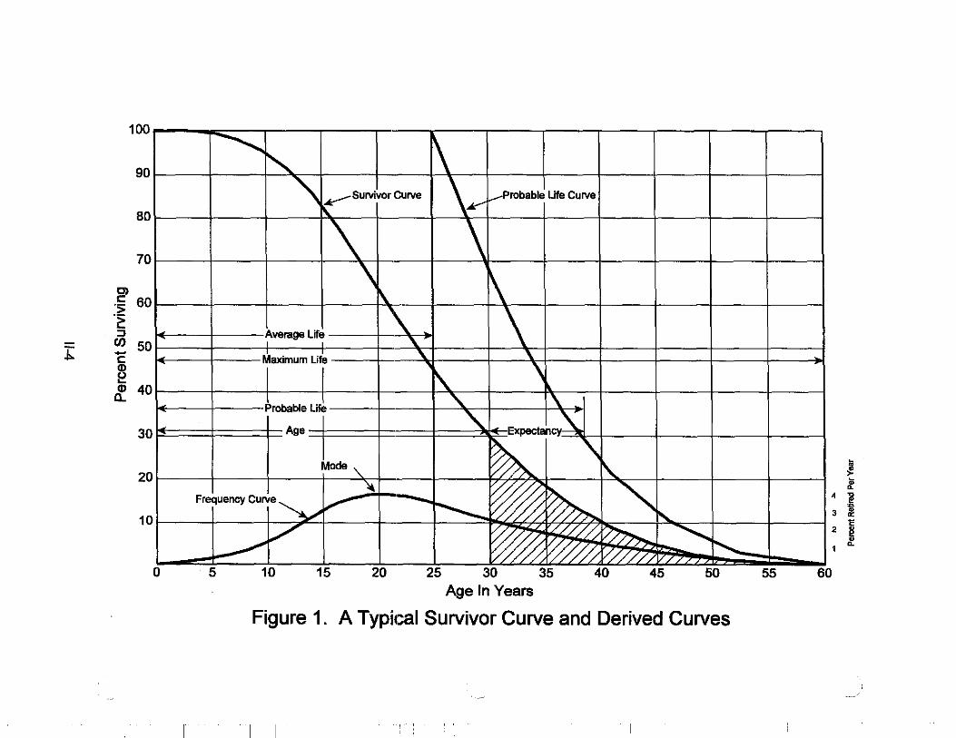
The survivor curve graphically depicts the amount of property existing at each age
throughout the life of an original group. From the survivor curve, the average life of the
group, the remaining life expectancy, the probable life, and the frequency curve can be
calculated. In Figure 1, a typical smooth survivor curve and the derived curves are
illustrated. The average life is obtained by calculating the area under the survivor curve,
from age zero to the maximum age, and dividing this area by the ordinate at age zero. The
remaining life expectancy at any age can be calculated by obtaining the area under the
curve, from the observation age to the maximum age, and dividing this area by the percent
surviving at the observation age. For example, in Figure 1 the remaining life at age 30 years
is equal to the crosshatched area under the survivor curve divided by 29.5 percent surviving
at age 30. The probable life at any age is developed by adding the age and remaining life.
If the probable life of the property is calculated for each year of age, the probable life curve
shown in the chart can be developed. The frequency curve presents the number of units
retired in each age interval and is derived by obtaining the differences between the amount
of property surviving at the beginning and at the end of each interval.
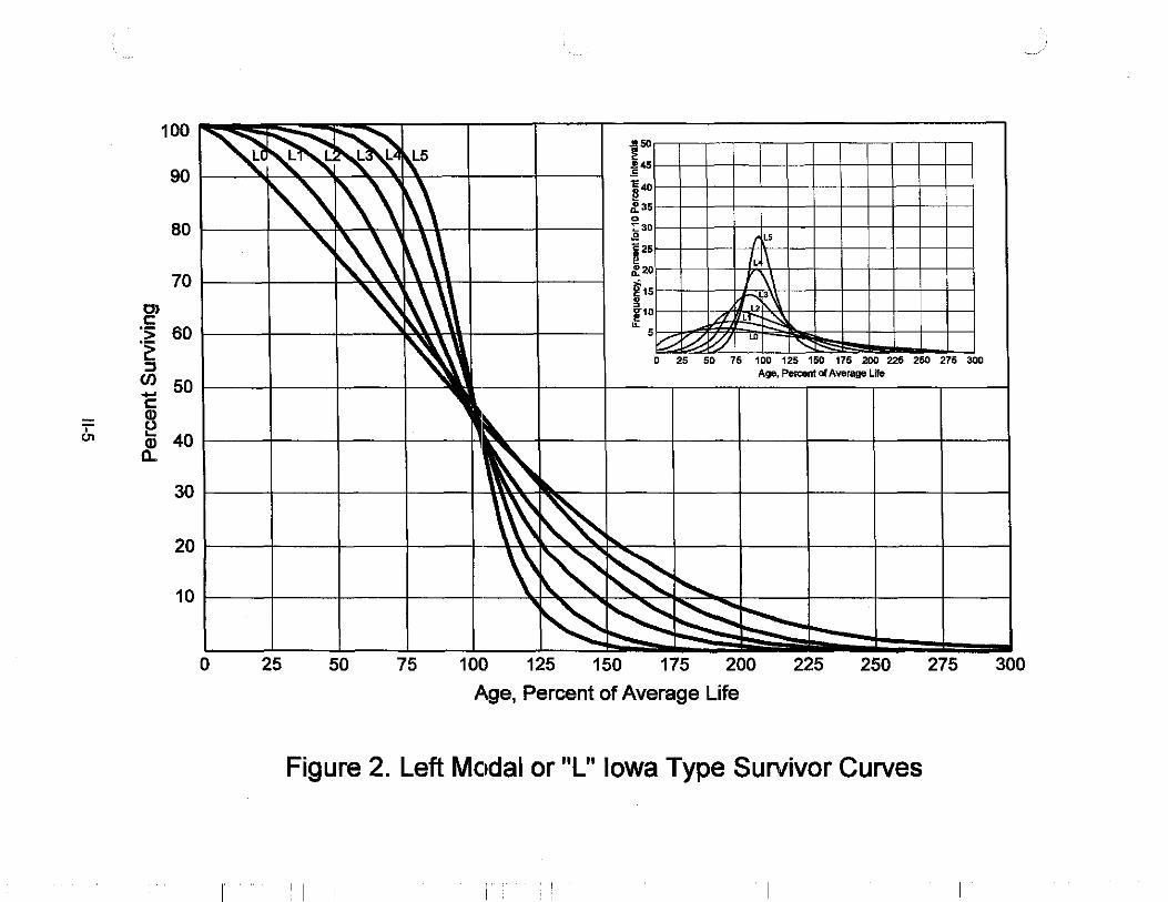
Iowa Type Curves. The range of survivor characteristics usually experienced by
utility and industrial properties is encompassed by a system of generalized survivor curves
known as the Iowa type curves. There are four families in the Iowa system, labeled in
accordance with the location of the modes of the retirements in relationship to the average
life and the relative height of the modes. The left moded curves, presented in Figure 2, are
those in which the greatest frequency of retirement occurs to the left of, or prior to, average
service life. The symmetrical moded curves, presented in Figure 3, are those in which the
11-3
.I>.
100
90
80
70
-~ 60 -~ :::i
"' 50 -~ Q; 40 a..
30
20
10
-
0
-.............. I\ !'...
"' ..,--survivor Curve \~ 1--Probable Life Curve
'
\ \ \ \ \.
Average Life '\ - \ I I " I I
" '\ Maximum Life
' I\. Probable Life ' \.
' Expectan~~ Age
~ \ Mode '\. ~
"" ~ ~ " Frequency Curve~ V" -r---... i....
v ~ -///7/ ~ ~ _,,, Wh r-...... r/////, ,. , >
5 10 15 20 25 30 35 - -40 -
45 --50 Age In Years
Figure 1. A Typic::al Survivor Curve and Derived Curves
I
- -
55
~ :f
4 !l 'll 3 0: c
2 ~ ~
60
100
90
80
70 O> c: ·s; 60 -~ ::J
(J) 50 -c: CD
T 0 01 Ci> 40
a..
30
20
10
0 25 50 75 100 125 150
1: .. "E40 ~ ,f 31 0 ;:30 .e
;
I
!2 ; 10 :_2,
~1 ! !'
15
11) ..
L5
L
I\\
·~ /1 L• -"-' ;V..- ~ 10 LO
' 0 25 50 75 100 125 150 175 200 226 250 275 300
Age, Percent Of Average Life
175 200 225 250 275
Age, Percent of Average Life
Figure 2. Left Modal or "L" Iowa Type Survivor Curves
I I I
300

100
90
80
70
Cl c: :~ 60 c: :J
Cl) - 50 c: (I)
T 0 ..... 40 Ol (I)
a_
30
20
10
0
~
!!-... ~~ ~86 s~ -~
~' ""X'' '\ ~ ~' ~ ' ' ~ ~ I
'
~
25 50 75
50 .. i4s ~40 " ~ 35 •• .. sao a 2s
" g 20 .. ~ ii' 15 ., J10 1
s ~ 5
'% ~~ ,...-~ ~ ~ D 25 50 75 100 125 150 175 200 225 250 275 300
Age, Percent of Average Liie
\ \
~ ~ ~ ~ ' \\ ~ ~ ~
100 125 150 175 200 225 250 275 300
Age, Percent of Average Life
Figure 3. Symmetrical or "S" Iowa Type Survivor Curves
I I I; I

greatest frequency of retirement occurs at average service life. The right moded curves,
presented in Figure 4, are those in which the greatest frequency occurs to the right of, or
after, average service life. The origin moded curves, presented in Figure 5, are those in
which the greatest frequency of retirement occurs at the origin, or immediately after age
zero. The letter designation of each family of curves (L, S, R or 0) represents the location
of the mode of the associated frequency curve with respect to the average service life. The
numerical subscripts represent the relative heights of the modes of the frequency curves
within each family.
The Iowa curves were developed at the Iowa State College Engineering Experiment
Station through an extensive process of observation and classification of the ages at which
industrial property had been retired. A report of the study which resulted in the
classification of property survivor characteristics into 18 type curves, which constitute three
of the four families, was published in 1935 in the form of the Experiment Station's Bulletin
125.1 These type curves have also been presented in subsequent Experiment Station
bulletins and in the text, "Engineering Valuation and Depreciation."2 In 1957, Frank V. B.
Couch, Jr., an Iowa State College graduate student, submitted a thesis3 presenting his
development of the fourth family consisting of the four 0 type survivor curves.
'Winfrey, Robley. Statistical Analyses of Industrial Property Retirements. Iowa State College, Engineering Experiment Station, Bulletin 125. 1935.
2Marston, Anson, Robley Winfrey and Jean C. Hempstead. Engineering Valuation and Depreciation, 2nd Edition. New York, McGraw-Hill Book Company. 1953.
3Couch, Frank V. B., Jr. "Classification of Type 0 Retirement Characteristics of Industrial Property." Unpublished M.S. thesis (Engineering Valuation). Library, Iowa State College, Ames, Iowa. 1957.
11-7

' co
100
Cl c:
90
80
70
·s: 60 ·~ :l
Cl) 50 -c: ~ O; 40
Cl..
30
20
10
0
~ ~~; .so ~R~R )\,R5 " j••
" ~\ N c4D
135 ~30 R5
'\ ~ ' ' .e C25
j R4
I·· /J R3
~ ~15 • f/ R2 ,
I !10 R1 \~
5 ~ ,\ ~ 1'...
D 25 50 75 100 125 150 175 200 225 250 275 300 Age, Percent Of Average Ufa
l' & \.
~\ \\. l\ \\\ :\. \ \..' ~ r--...._
-
25 - -
50 -
75 100 125 150 175 200 225 250 275 300
A!~e. Percent of Average Life
Figure 4. Right Modal or "R" Iowa Type Survivor Curves
I i ! I I . I

100
90
80
70
Cl c
·s;: 60 -~ :::J (/) 50 -c
G>
' e 40 co G> 0..
30
20
10
~ 1120 ~ .!! 18
~ " ~·· ir_14 0
: 12
\ ~~ JO ........ r: 10
~ ~ 'Z' ~ . -....
\\ ~ ii' 6 03
~ 01 ~ e-• "-..: !"- ......... ' u. ~ 2
\ ~"' ~ 0 25 50 75 100 125 150 175 200 225 250 275 300
Age, Percent of Average Life
o~ ~2'\ ,Jo.c
-~ .. "'-~ ~~ " ........... ~ '"
~ ~ -
"' --- -
0 -25 50 75 - - -100 125 150 175 200 225 250 275 300 Age, Percent of Average Life
Figure 5. Origin ~Jlodal or "O" Iowa Type Survivor Curves
I I 11
" I:
--.,-'

Retirement Rate Method of Analvsis
The retirement rate method is an actuarial method of deriving survivor curves using
the average rates at which property of each age group is retired. The method
relates to property groups for which aged accounting experience is available or for which
aged accounting experience is developed by statistically aging unaged amounts and is the
method used to develop the original stub survivor curves in this study. The method (also
known as the annual rate method) is illustrated through the use of an example in the
following text, and is also explained in several publications, including "Statistical Analyses
of Industrial Property Retirements,"4 "Engineering Valuation and Depreciation,"5 and
"Depreciation Systems."6
The average rate of retirement used in the calculation of the percent surviving for
the survivor curve (life table) requires two sets of data: first, the property retired during a
period of observation, identified by the property's age at retirement; and second, the
property exposed to retirement at the beginnings of the age intervals during the same
period. The period of observation is referred to as the experience band, and the band of
years which represent the installation dates of the property exposed to retirement during
the experience band is referred to as the placement band. An example of the calculations
used in the development of a life table follows. The example includes schedules of annual
aged property transactions, a schedule of plant exposed to retirement, a life table, and
illustrations of smoothing the stub survivor curve.
4Winfrey, Robley, Supra Note 1. 5Marston, Anson, Robley Winfrey, and Jean C. Hempstead, Supra Note 2. 6Wolf, Frank K. and W. Chester Fitch. Depreciation Systems. Iowa State University
Press. 1994
11-10

Schedules of Annual Transactions in Plant Records. The property group used to
illustrate the retirement rate method is observed forthe experience band 2003-2012 during
which there were placements during the years 1998-2012. In order to illustrate the
summation of the aged data by age interval, the data were compiled in the manner
presented in Schedules 1 and 2 on pages 11-12 and 11-13. In Schedule 1, the year of
installation (year placed) and the year of retirement are shown. The age interval during
which a retirement occurred is determined from this information. In the example which
follows, $10,000 of the dollars invested in 1998 were retired in 2003. The $10,000
retirement occurred during the age interval between 4Yz and 5Yz years on the basis that
approximately one-half of the amount of property was installed prior to and subsequent to
July 1 of each year. That is, on the average, property installed during a year is placed in
service at the midpoint of the year for the purpose of the analysis. All retirements also are
stated as occurring at the midpoint of a one-year age interval of time, except the first age
interval which encompasses only one-half year.
The total retirements occurring in each age interval in a band are determined by
summing the amounts for each transaction year-installation year combination for that age
interval. For example, the total of $143,000 retired for age interval 4Yz-5Yz is the sum of
the retirements entered on Schedule 1 immediately above the stairstep line drawn on the
table beginning with the 2003 retirements of 1998 installations and ending with the 2012
retirements of the 2007 installations. Thus, the total amount of 143 for age interval 4 Yz-5Yz
equals the sum of:
10+12+13+11+13+13+15+17+19 + 20.
In Schedule 2, other transactions which affect the group are recorded in a similar
manner. The entries illustrated include transfers and sales. The entries which are credits
to the plant account are shown in parentheses. The items recorded on this schedule
11-11

;-~
N
Experience Band 2003-2012
Year Placed
(1)
1998 1999 2000 2001 2002 2003 2004 2005 2006 2007 2008 2009 2010 2011 2012
Total
2003 (2)
10 11 11 8 9 4
53 ~
2004 (3)
11 12 12 9
10 9 5
68
I I
SCHEDULE 1. RETIREMENTS FOR EACH YEAR 2003-2012 SUMMARIZED BY AGE INTERVAL
Placement Band 1998-2012 Retinaments, Thousands of Dollars
During Year Total During Age 2005 2006 2007 2008 2009 2010 2011 2012 Age Interval Interval
(4) (5) (6) (7) (8) (9) (10) (11) (12) (13)
12 13 14 16 23 24 25 26 26 13%-14112 13 15 16 18 20 21 22 19 44 12112-13112 13 14 16 17 19 21 22 18 64 11%-12112 10 11 11 13 14 15 16 17 83 10112-11112 11 12 13 14 16 17 19 20 93 9%-10112 10 11 12 13 14 15 16 20 105 8%-9112 11 12 13 14 15 16 18 20 113 7112-8112
6 12 13 15 16 17 19 19 124 6%-71h 6 13 15 16 17 19 19 131 5%-6112
7 14 16 17 19 20 143 4%-51h 8 18 20 22 23 146 3112-4112
9 20 22 25 150 2%-3Y, 11 23 25 151 1%-2%
11 24 153 %-1% _n ___§Q 0-'h
86 106 128 157 196 231 273 308 1,606 = = = =
. __ /
I:

' ~ w
SCHEDULE 2. OTHER TRANSACTIONS FOR EACH YEAR 2003-2012 SUMMARIZED BY AGE INTERVAL
Experience Band 2003-2012 Placement Band 1998-2012 Acquisitions, Transfers and Sales, Thousands of Dollars
Year During Year Total During Age Placed 2003 2004 2005 2006 2007 2008 2009 2010 2011 2012 Age Interval Interval
(1) (2) (3) (4) (5) {13) (7) (8) (9) (10) (11) (12) (13)
1998 - '" - 60° - - - - 13%-1411, 1999 - - - - - - - - - - 12%-1311, 2000 - - - - - - - - - - 11 %-1211, 2001 - - - - - - - (5)b 60 10%-11% 2002 - - - - - - 6" - - - 911,-1011, 2003 - - - - - - - - - (5) 8%-911, 2004 - - - - - - - - 6 7%-8% 2005 - - - - - - - - - 6%-7Y, 2006 - - - - (12)b - - 5%-6% 2007 - - 22· - 4}~5Y,
2008 - - (19)b - - 10 3Y.-4Y:. 2009 - - - 2}~3Y,
2010 - (102)° (121) 1%-2% 2011 %-1 Y:z 2012 -- 0-Y,
Total - - - - - - 60 ~) 22 (102) ( 50) = = = = ·= =
•Transfer Affecting Exposures at Beginning of Year b Transfer Affecting Exposures at End of Year 0
Sale with Continued Use Parentheses denote Credit amount.
I I i I I

are not !ota!ed with the retirements bu! are used in developing the exposures at the beginning
of each age interval.
Schedule of Plant Exposed to Retirement. The development of the amount of plant
exposed to retirement at the beginning of each age interval is illustrated in Schedule 3 on
page 11-15.
The surviving plant at the beginning of each year from 2003 through 2012 is recorded
by year in the portion of the table headed "Annual Survivors at the Beginning of the Year."
The last amount entered in each column is the amount of new plant added to the group during
the year. The amounts entered in Schedule 3 for each successive year following the
beginning balance or addition are obtained by adding or subtracting the net entries shown on
Schedules 1 and 2. For the purpose of determining the plant exposed to retirement,
transfers-in are considered as being exposed to retirement in this group at the beginning of
the year in which they occurred, and the sales and transfers-out are considered to be
removed from the plant exposed to retirement at the beginning of the following year. Thus,
the amounts of plant shown at the beginning of each year are the amounts of plant from each
placement year considered to be exposed to retirement at the beginning of each successive
transaction year. For example, the exposures for the installation year 2008 are calculated in
the following manner:
Exposures at age 0 = amount of addition Exposures at age Y:i = $750,000 - $ 8,000 Exposures at age 1Y:i = $742,000- $18,000 Exposures at age 2Y:i = $724,000 - $20,000 - $19,000 Exposures at age 3Y:i = $685,000 - $22,000
= $750,000 = $742,000 = $724,000 = $685,000 = $663,000
For the entire experience band 2003-2012, the total exposures at the beginning of an
age interval are obtained by summing diagonally in a manner similar to the summing
11-14
. \ I

~~
SCHEDULE 3. PLANT EXPOSED TO RETIREMENT JANUARY 1 OF EACH YEAR 2003-2012
SUMMARIZED BY AGE INTERVAL
Experience Band 2003-2012 Placement Band 1998-2012
Exposur,es, Thousands of Dollars Total at
Year 8onyal ;;iyrvjv~>lli a! !ll!i! !;!!lgiooiog Qf lll!i! Y!i!i!C Beginning of Age Placed 2003 2004 2005 2006 2007 2008 2009 2010 2011 2012 Age Interval Interval
(1) (2) (3) (4) (5) (6) (7) (8) (9) (10) (11) (12) ('13)
1998 255 245 234 222 209 195 239 216 192 167 167 13Y.-14Y,
1999 279 268 256 243 228 212 194 174 153 131 323 12Y.-13Y, 2000 307 296 284 271 257 241 224 205 184 162 531 11%-12Y. 2001 338 330 321 311 300 289 276 262 242 226 823 10Yz-11Y, 2002 376 367 357 346 334 321 307 297 280 261 1,097 9Y.-10Y.
2003 4203 416 407 397 386 374 361 347 332 316 1,503 8~'2-9~
;-- 2004 4603 455 444 432 419 405 390 374 356 1,952 7~'2-8% ~ 2005 510• 504 492 479 464 448 431 412 2,463 6%-7Y, 01
2006 580" 574 561 546 530 501 482 3,057 5~t2-6Y2
2007 6603 653 639 623 628 609 3,789 4~1z-5~
2008 7503 742 724 685 663 4,332 3~'2-4%
2009 850· 841 821 799 4,955 2%-3% 2010 960" 949 926 5,719 1 Ya-2Ya 2011 1,080• 1,069 6,579 Y,-1 y,
2012 1,220· _L490 0-Y.
Total 1,975 2,382 2,824 3,318 3,872 4494 5,247 6,017 6,852 7,799 44.780
• Additions during the year.
I I 'I. i I I

of the retirements during an age interval (Schedule 1). For example, the figure of 3,789,
shown as the total exposures at the beginning of age interval 4%-5%, is obtained by
summing:
255 + 268 + 284 + 311 + 334 + 374 + 405 + 448 + 501 + 609.
Original Life Table. The original life table, illustrated in Schedule 4 on page 11-17,
is developed from the totals shown on the schedules of retirements and exposures,
Schedules 1 and 3, respectively. The exposures at the beginning of the age interval are
obtained from the corresponding age interval of the exposure schedule, and the
retirements during the age interval are obtained from the corresponding age interval of the
retirement schedule. The retirement ratio is the result of dividing the retirements during the
age interval by the exposures at the beginning of the age interval. The percent surviving
at the beginning of each age interval is derived from survivor ratios, each of which equals
one minus the retirement ratio. The percent surviving is developed by starting with 100%
at age zero and successively multiplying the percent surviving at the beginning of each
iniervai by the survivor ratio, i.e., one minus the retirement ratio for that age interval. The
calculations necessary to determine the percent surviving at age 5Y:i are as follows:
Percent surviving at age 4Y:i = 88.15 Exposures at age 4% = 3,789,000 Retirements from age 4% to 5Y:i = 143,000 Retirement Ratio = 143,000 + 3,789,000 = 0.0377 Survivor Ratio = 1.000 - 0.0377 = 0.9623 Percent surviving at age 5Y:i = (88.15) x (0.9623) = 84.83
The totals of the exposures and retirements (columns 2 and 3) are shown for the
purpose of checking with the respective totals in Schedules 1 and 3. The ratio of the total
retirements to the total exposures, other than for each age interval, is meaningless.
11-16

\
' SCHEDULE 4. ORIGINAL LIFE TABLE CALCULATED BY THE RETIREMENT RATE METHOD
Experience Band 2003-2012 Placement Band 1998-2012
(Exposure and Retirement Amounts are in Thousands of Dollars)
Age at Exposures at Retirements Beginning of Beginning of During Age Retirement Survivor
Interval Age Interval Interval Ratio Ratio (1) (2) (3) (4) (5)
0.0 7,490 80 0.0107 0.9893
0.5 6,579 153 0.0233 0.9767
1.5 5,719 151 0.0264 0.9736
2.5 4,955 150 0.0303 0.9697
3.5 4,332 146 0.0337 0.9663
4.5 3,789 143 0.0377 0.9623
5.5 3,057 131 0.0429 0.9571
6.5 2,463 124 0.0503 0.9497
7.5 1,952 113 0.0579 0.9421
8.5 1,503 105 0.0699 0.9301
9.5 1,097 93 0.0848 0.9152
•n " Q')~ o~ n 1nnn n onn"I 1v.v U<.<J V<J Vo IVVQ V,UUO I
11.5 531 64 0.1205 0.8795
12.5 323 44 0.1362 0.8638
13.5 167 -2§ 0.1557 0.8443
Total 44,780 1,606
Column 2 from Schedule 3, Column 12, Plant Exposed to Retirement. Column 3 from Schedule 1, Column 12, Retirements for Each Year. Column 4 = Column 3 Divided by Column 2. Column 5 = 1.0000 Minus Column 4.
Percent Surviving at Beginning of Age Interval
(6)
100.00
98.93
96.62
94.07
91.22
88.15
84.83
81.19
77.11
72.65
67.57 Q.C OA u 1.0--t
55.60
48.90
42.24
35.66
Column 6 = Column 5 Multiplied by Column 6 as of the Preceding Age Interval.
11-17

The original survivor curve is plotted from !he original !ife table (column 6, Schedule
4). When the curve terminates at a percent surviving greaterthan zero, it is called a stub
survivor curve. Survivor curves developed from retirement rate studies generally are stub
curves.
Smoothing the Original Survivor Curve. The smoothing of the original survivor curve
eliminates any irregularities and serves as the basis for the preliminary extrapolation to
zero percent surviving of the original stub curve. Even if the original survivor curve is
complete from 100 percent to zero percent, it is desirable to eliminate any irregularities, as
there is still an extrapolation for the vintages which have not yet lived to the age at which
the curve reaches zero percent. In this study, the smoothing of the original curve with
established type curves was used to eliminate irregularities in the original curve.
The Iowa type curves are used in this study to smooth those original stub curves
which are expressed as percents surviving at ages in years. Each original survivor curve
was compared to the Iowa curves using visual and mathematical matching in order to
determine the better fitting smooth curves. In Figures 6, 7, and 8, the original curve
developed in Schedule 4 is compaied with the L, S, and R Iowa type curves which rnost
nearly fit the original survivor curve. In Figure 6, the L 1 curve with an average life between
12 and 13 years appears to be the best fit. In Figure 7, the SO type curve with a 12-year
average life appears to be the best fit and appears to be betterthan the L 1 fitting. In Figure
8, the R1 type curve with a 12-year average life appears to be the best fit and appears to
be better than either the L 1 or the SO. In Figure 9, the three fittings, 12-L 1, 12-SO and 12-
R1 are drawn for comparison purposes. II is probable that the 12-R1 Iowa curve would be
selected as the most representative of the plotted survivor characteristics of the group,
assuming no contrary relevant factors external to the analysis of historical data.
11-18

100
90
BO
70
~ 60 .
> > 0:: :::J "' 50 I
;- ,_ ..... z <O "' u
0:: ~ I.IQ
30
20
10
x
0
~
~ ~ ~ ~ ~ I~
\ .
.
5
I I
FIGURE 6. ILLUSTAATION OF THE HATCHING OF AN OAIGINAL SURVIVOR CURVE HITH AN LI IOWA TYPE CURVE
OAIGINAL CUAVE: X 2003-2012 EXPERIENCE; 1996-2012 PLACEMENTS
fix l l-L1 '
~~ 2-L1
)OWA 13 L1
"'~ I~ "' ~ ~ ~ ~ "" ~ ~ ~
"""-~ ~ :::----
10 15 20 25 30 RGE IN YEARS
11 I.

100
90
BO
70
0 z 60
> > a: :::J Ill so I
T >"' z 0 w u
a: ll: q
3,
21
I
l
l
I
x~
" ~ ~ ~ ~ ~
'\
0 5
I '
FIGURE 7. ILLUSTRATION OF THE MATCHING OF AN ORIG1NAL SURVIVOR CURVE WITH AN SO IOWA TYPE CURVE
ORIGINAL CURVE: X 2003-2012 EXPERIENCE: 1996-2012 PLACEMENTS
~ 11-~ o
~0 i 12-So
"\. )OWR 13-So
'\ ~ ~~ ~
"' ~~ ~ ~ ~ ~ ~ ~ ~
10 IS 20 25 30 AGE IN YEARS
j
r I Ii

___ /
100
tJ z > > a: :J Ill
' ,_
"' z ~ w
u a: w ._
~ FIGURE 8. ILLUSTRATION OF THE MATCHING OF AN ORIGINAL
~ SURVIVOR CURVE WITH AN Al IOWA TlPE CURVE
~ ~
ORIGINAL CURVE: X 2003-2012 EXPERIENCE: 1996-2012 PLACEMENTS
'
~ ~ I
~ ~~ 1 -R1
\:\ OWA 12-R
~/row 13-Ri
\ ~~ \\ ~
\ ~~ ~ ~' ~~ "-
90
80
70
60
50
ij0
31
21
~ ~ '-------0 5 10 15 20 25 30
RGE IN YEARS
I I i I I

100
" z > > a: ::J
"' ~ ;- z
'" N u N a:
'" '-
~ ~ FJ~E 9. ILLUSTARTJON OF THE MATCHING OF AN ORJGINRL
SUAVJVCFI CURVE HI TH LI. SO ANO Al !OHR TTPE CURVES
~
~ ORIGINAL CURVE: X 2003-2012 EXPERIENCE: 1998-2012 PLACEMENTS
~ & ~ tx._ ,!DWI 12-Rt
/
" ~~ R 12-So
R 12-L t
·~
~ ~ ' ~
90
ao
70
60
50
40
30
20
~ "-""' ~ ----------
10
0 5 10 15 20 25 30 FlGE IN YEARS
I . i I Ii

Service Life Considerations
The service life estimates were based on judgment which considered a number of
factors. The primary factors were the statistical analyses of data; current Company policies
and outlook as determined during conversations with management; and the survivor curve
estimates from previous studies of this company and other electric companies.
For 30 of the plant accounts and subaccounts for which survivor curves were
estimated, the statistical analyses using the retirement rate method resulted in good to
excellent indications of the survivor patterns experienced. These accounts represent 51
percent of depreciable plant. Generally, the information external to the statistics led to no
significant departure from the indicated survivor curves for the accounts listed below. The
statistical support for the service life estimates is presented in the section beginning on
page 111-9.
ELECTRIC PLANT Steam Plant
311.00 315.00 316.00
Structures and Improvements Accessory Electric Equipment Miscellaneous Power Plant Equipment
Transmission Plant 352.00 Structures and Improvements 353.00 Station Equipment 355.00 Poles and Fixtures 356.00 Overhead Conductors and Devices
Distribution Plant 361.00 Structures and Improvements 361.05 Land Improvements 362.00 Station Equipment 364.00 Poles, Towers and Fixtures 365.00 Overhead Conductors and Devices 366.00 Underground Conduit 367.00 Underground Conductors and Devices 368.01 Line Transformers - Other Equipment 368.02 Line Transformers - Conventional 368.03 Line Transformers - Padmount 369.01 Services - Overhead 369.02 Services - Underground
11-23

370.01 371.00 373.00
General Plant 390.01 392.01 392.02 392.03 392.04 392.05 392.06 397.01
Meters Installations on Customer Premises Street Lighting and Signal Systems
Structures and Improvements Transportation Equipment - Subunit Transportation Equipment - Cars Transportation Equipment - Light Trucks Transportation Equipment - Medium Trucks Transportation Equipment - Heavy Trucks Transportation Equipment - Trailers Communication Equipment - Towers
Electric Plant Account 362.00 Station Equipment, is used to illustrate the manner
in which the study was conducted for the groups in the preceding list. Aged plant
accounting data for the distribution plant have been compiled for the years 1946 through
2012. These data have been coded in the course of the Company's normal record keeping
according to account or property group, type of transaction, year in which the transaction
took place, and year in which the electric plant was placed in service. The retirements,
other plant transactions, and plant additions were analyzed by the retirement rate method.
The survivor curve estimate is based on the statistical indications for the period
1946 through 2012. The Iowa 45-R2 is a reasonable fit of the stub original survivor of
station equipment. The 45-year service life is within the typical service life range of 35 to
55 years for station equipment. The 45-year life reflects the Company's plans to continue
to upgrade equipment when necessary with expectations that some assets based on
demand could be in service well beyond the average life.
Account 364.00, Poles, Towers and Fixtures, is another large account for which the
statistical analyses was a strong indicator of life characteristics. Aged plant accounting
data have been compiled for the years 1950 through 2012. The Iowa 50-R2 is a good fit
of the stub original curve of poles. The 50-year service life reflects the statistical
11-24

indications, Company plans to replace poles primarily due to wear and tear as well as load
upgrades, and the range of estimates of other electric utilities for poles.
Inasmuch as production plant consists of large generating units, the life span
technique was employed in conjunction with the use of interim survivor curves which reflect
interim retirements that occur prior to the ultimate retirement of the major unit. An interim
survivor curve was estimated for each plant account, inasmuch as the rate of interim
retirements differ from account to account. The interim survivor curves estimated for
steam and other production plant related to Black Hills Power stations were based on the
retirement rate method.
The life span estimates for power generating stations were the result of considering
experienced- life spans of similar generating units, the age of surviving units, general
operating characteristics of the units, major refurbishing, and discussions with
management personnel concerning the probable long-term outlook for the units. Final
decisions as to date of retirement will be determined by management on a unit by unit
basis.
The life span estimates for the steam, base-load units is 45-61 years, which is
within the typical range of life spans for such units. The life span estimates for other
production units is 45-54 years which is slightly long for combustion turbines and diesel
units.
A summary of the year in service, life span and probable retirement year for each
power production unit follows:
Depreciable Group
Steam Production Plant Ben French Neil Simpson I Neil Simpson II
Year in Service
1962 1969 1998
11-25
Probable Retirement
Year Life Span
2014 52 2014 45 2045 47

Probable Year in Retirement
Depreciable Group Service Year Life Span
Osage 1953 2014 61 Wygen 3 2010 2060 50 Wyodak 1991 2039 48
Other Production Plant Ben French CT 1977 2030 53 Lange CT 2003 2048 45 Neil Simpson CT 2001 2046 45 Ben French Diesel 1966 2020 54
The survivor curve estimates for the remaining accounts were based on judgment
incorporating the statistical analyses and previous studies for this and other electric and
gas utilities.
Salvage Analysis
The estimates of net salvage by account were based in part on historical data
compiled through 2012. Cost of removal and salvage were expressed as percents of the
original cost of plant retired, both on annual and three-year moving average bases. The
most recent fivecyear average also was calculated for consideration. The net salvage
estimates by account are expressed as a percent of the original cost of plant retired.
Net Salvage Considerations
The estimates of future net salvage are expressed as percentages of surviving plant
in service, i.e., all future retirements. In cases in which removal costs are expected to
exceed salvage receipts, a negative net salvage percentage is estimated. The net salvage
estimates were based on judgment which incorporated analyses of historical cost of
removal and salvage data, expectations with respect to future removal requirements and
markets for retired equipment and materials.
The analyses of historical cost of removal and salvage data are presented in the
section titled "Net Salvage Statistics" for the plant accounts for which the net salvage
estimate relied partially on those analyses.
11-26
)

Statistical analyses of historical data for the period 1997 through 2012 contributed
significantly toward the net salvage estimates for 20 plant accounts, representing 83
percent of the depreciable plant, as follows:
ELECTRIC PLANT Steam Production Plant
312.01 Boiler Plant Equipment 314.00 Turbogenerators 316.00 Miscellaneous Power Plant Equipment
Other Production Plant 342.00 Fuel Holders and Accessories 344.01 Generators
Transmission Plant 352.00 Structures and Improvements 353.00 Station Equipment 355.00 Poles and Fixtures
Distribution Plant 362.00 364.00 365.00 366.00 367.00 369.01 369.02 370.01 370.04 371.00 373.00
General Plant 390.01
Station Equipment Poles, Towers and Fixtures Overhead Conductors and Devices Underground Conduit Underground Conductors and Devices Services - Overhead Services - Underground Meters Meters-AMI Installations on Customer Premises Street Lighting and Signal Systems
Structures and Improvements
The Electric Plant analyses for Account 365.00, Overhead Conductors and Devices,
is used to illustrate the manner in which the study was conducted for the groups in the
preceding list. Net salvage data for the period 1997 through 2012 were analyzed for this
account. The data include cost of removal, gross salvage and net salvage amounts and
each of these amounts is expressed as a percent of the original cost of regular retirements.
11-27
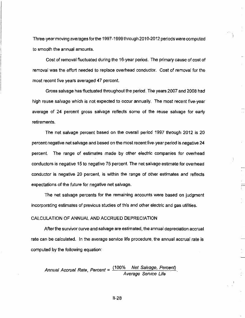
Three-year moving averages for the 1997-1999 through 2010-2012 periods were computed
to smooth the annual amounts.
Cost of removal fluctuated during the 16-year period. The primary cause of cost of
removal was the effort needed to replace overhead conductor. Cost of removal for the
most recent five years averaged 4 7 percent.
Gross salvage has fluctuated throughout the period. The years 2007 and 2008 had
high reuse salvage which is not expected to occur annually. The most recent five-year
average of 24 percent gross salvage reflects some of the reuse salvage for early
retirements.
The net salvage percent based on the overall period 1997 through 2012 is 20
percent negative net salvage and based on the most recent five-year period is negative 24
percent. The range of estimates made by other electric companies for overhead
conductors is negative 15 to negative 75 percent. The net salvage estimate for overhead
conductor is negative 20 percent, is within the range of other estimates and reflects
expectations of the future for negative net salvage.
The net salvage percents for the remaining accounts were based on judgment
incorporating estimates of previous studies of this and other electric and gas utilities.
CALCULATION OF ANNUAL AND ACCRUED DEPRECIATION
After the survivor curve and salvage are estimated, the annual depreciation accrual
rate can be calculated. In the average service life procedure, the annual accrual rate is
computed by the following equation:
Annual Accrual Rate, Percent= (100% Net Salvage, Percent) Average Service Life
11-28

The calculated accrued depreciation for each depreciable property group represents that
portion of the depreciable cost of the group which will not be allocated to expense through
future depreciation accruals if current forecasts of life characteristics are used as a basis
for straight line depreciation accounting.
The accrued depreciation calculation consists of applying an appropriate ratio to the
surviving original cost of each vintage of each account, based upon the attained age and
the estimated survivor curve. The accrued depreciation ratios are calculated as follows:
Ratio = (1 _ Average Remaining Life Expectancy ) (1 _Net Salvage, Percent). Average Service Life
The application of these procedures is described for a single unit of property and
a group of property units. Salvage is omitted from the description for ease of application.
Single Unit of Property
The calculation of straight line depreciation for a single unit of property is
straightforward. For example, if a $1,000 unit of property attains an age of four years and
has a life expectancy of six years, the annual accrual over the total life is:
$1,000 = $100 per year. (4 + 6)
The accrued depreciation is:
$1,000 (1 - _§__) = $400. 10
Group Depreciation Procedures
When more than a single item of property is under consideration, a group procedure
for depreciation is appropriate because normally all of the items within a group do not have
11-29

identical service lives, but have lives that are dispersed over a range of time. There are
two primary group procedures, namely, average service life and equal life group.
Remaining Life Annual Accruals. For the purpose of calculating remaining life
accruals as of December 31, 2012 the depreciation reserve for each plant account is
allocated among vintages in proportion to the calculated accrued depreciation for the
account. Explanations of remaining life accruals and calculated accrued depreciation
follow. The detailed calculations as of December 31, 2012 are set forth in the Results of
Study section of the report.
Average Service Life Procedure. In the average service life procedure, the
remaining life annual accrual for each vintage is determined by dividing future book
accruals (original cost less book reserve) by the average remaining life of the vintage. The
average remaining life is a directly weighted average derived from the estimated future
survivor curve in accordance with the average service life procedure.
The calculated accrued depreciation for each depreciable property group represents
that portion of the depreciable cost of the group which would not be allocated to expense
through future depreciation accruals, if current forecasts of life characteristics are used as
the basis for such accruals. The accrued depreciation calculation consists of applying an
appropriate ratio to the surviving original cost of each vintage of each account, based upon
the attained age and service life. The straight line accrued depreciation ratios are
calculated as follows for the average service life procedure:
Average Remaining Life Ratio = 1 -
Average Service Life
11-30

CALCULATION OF ANNUAL AND ACCRUED AMORTIZATION
Amortization, as defined in the Uniform System of Accounts, is the gradual
extinguishment of an amount in an account by distributing such amount over a fixed period,
over the life of the asset or liability to which it applies, or over the period during which it is
anticipated the benefit will be realized. Normally, the distribution of the amount is in equal
amounts to each year of the amortization period.
The calculation of annual and accrued amortization requires the selection of an
amortization period. The amortization periods used in this report were based on judgment
which incorporated a consideration of the period during which the assets will render most
of their service, the amortization periods and service lives used by other utilities, and the
service life estimates previously used for the asset under depreciation accounting.
Amortization accounting is appropriate for certain General Plant accounts that
represent numerous units of property, but a very small portion of depreciable electric and
gas plant in service. The accounts and their amortization periods are as follows:
Account
GENERAL PLANT 391.01 Office Furniture and Equipment 391.03 Computer Hardware 391.05 System Development 393.00 Stores Equipment 394.00 Tools, Shop and Garage Equipment 395.00 Laboratory Equipment 397.00 Communication Equipment 398.00 Miscellaneous Equipment
Amortization Period, Years
20 5 5
20 25 25 20 20
For the purpose of calculating annual amortization amounts as of December 31,
2012, the book or ratemaking book depreciation reserve for each plant account or
subaccount is assigned or allocated to vintages. The reserve assigned to vintages with an
age greater than the amortization period is equal to the vintage's original cost. The
11-31

remaining reserve is allocated among vintages with an age iess than ihe amortization
period in proportion to the calculated accrued amortization. The calculated accrued
amortization is equal to the original cost multiplied by the ratio of the vintage's age to its
amortization period. The annual amortization amount is determined by dividing the future
amortizations (original cost less allocated book reserve) by the remaining period of
amortization for the vintage.
11-32

111-1 PART Ill. RESULTS OF STUDY

PART Ill. RESULTS OF STUDY
QUALIFICATION OF RESULTS
The calculated annual depreciation accrual amounts and rates are the principal
results of the study. Continued surveillance and periodic revisions are normally required
to maintain continued use of appropriate annual depreciation accrual rates. An assumption
that accrual rates can remain unchanged over a long period of time implies a disregard for
the inherent variability in service lives and salvage and for the change of the composition
of property in service. The annual accrual rates were calculated in accordance with the
straight line remaining life method of depreciation using the average service life procedure
based on estimates which reflect considerations of current historical evidence and
expected future conditions.
The annual depreciation accrual rates are applicable specifically to the electric, gas
and common plant in service as of December 31, 2012. For most plant accounts, the
application of such rates to future balances that reflect additions subsequent to December
31, 2012, is reasonable for a period of three to five years.
DESCRIPTION OF STATISTICAL SUPPORT
The service life and salvage estimates were based on judgment which incorporated
statistical analyses of retirement data, discussions with management and consideration of
estimates made for other electric utility companies. The results of the statistical analyses
of service life are presented in the section titled "Service Life Statistics''.
The estimated survivor curves for each account are presented in graphical form.
The charts depict the estimated smooth survivor curve and original survivor curve(s), when
applicable, related to each specific group. For groups where the original survivor curve
was plotted, the calculation of the original life table is also presented.
The analyses of salvage data are presented in the section titled, "Net Salvage
Statistics". The tabulations present annual cost of removal and salvage data, three-year
111-2

moving averages and the most recent five-year average. Data are shown in dollars and
as percentages of the original cost retired.
DESCRIPTION OF DEPRECIATION TABULATIONS
Summaries of the results of the study, as applied to the original cost of electric plant
as of December 31, 2012, are presented on pages 111-4 through 111-8 of this report. The
schedule sets forth the original cost, the book depreciation reserve, future accruals, the
calculated annual depreciation rate and amount, and the composite remaining life related
to electric plant.
The tables of the calculated annual depreciation accruals are presented in account
sequence in the section titled "Depreciation Calculations." The tables indicate the
estimated survivor curve and salvage percent for the account and set forth, for each
installation year, the original cost, the calculated accrued depreciation, the allocated book
reserve, future accruals, the remaining life and the calculated annual accrual amount.
111-3

BLACK HILLS POWER
SUMMARY OF ESTIMATED SUR'lllVOR CURVES, NET SALVAGE, ORIGINAL COST, BOOK DEPRECIATION RESERVE ANO CALCULATED ,ANNUAL DEPRECIATION ACCRUAL RA TES AS OF DECEMBER 31, 2012
NET BOOK CALCULATED ANNUAL COMPOSITE SURVIVOR SALVAGE ORIGINAL DEPRECIATION FUTURE ACCRUAL ACCRUAL REMAINING
ACCOUNT CURVE PERCENT COST RESERVE ACCRUALS AMOUNT RATE UFE
(11 (21 (31 (41 (51 (6) (7) (BF{7)/(4) (9}9'.6)/(7)
STEAM PRODUCTION PLANT
BEN FRENCH STATION 311.00 STRUCTURES AND IMPROVEMENTS 80-R1.5 (28) 2251,067.03 2,470,217 411,149 225,045 10.00 1.8 312.01 BOILER PLANT EQUIPMENT 55-S0.5 (281 6,842,535.53 6,971,855 1,786.590 985,304 14.40 1.8 314.00 TURBOGENERATOR UNITS 55-S0.5 (281 3,956,115.75 3,267,891 1,795,937 987.811 24.97 1.8 315.00 ACCESSORY ELECTRIC EQUIPMENT 65-R2.5 (281 756,487.01 817,196 151,107 83,050 10.98 1.8 316.00 MISCELLANEOUS POWER PLANT EQUIPMENT 45.SO (28) 461,437.84 529,424 61.216 33.837 7.33 1.8
TOTAL BEN FRENCH STATION 14.267,643.16 14,056,583 4,205,999 2,315,047 16.23 1.8
NEIL SIMPSON I 311.00 STRUCTURES AND IMPROVEMENTS 81J-R1.5 (13) 2,263,790.00 2,055,490 502,593 275,250 12.16 1.8 312.01 BOILER PLANT EQUIPMENT 55-S0.5 (13) 14,327 ,824.99 10,348,851 5,841,591 3,210,557 22.41 1.8 314.00 TURBOGENERATOR UNITS 55-S0.5 (13) 3,916,967.11 2,797,900 1,628,273 896,130 22.88 1.8 315.00 ACCESSORY ELECTRIC EQUIPMENT 65-R2.5 {13) 1,334,432.06 622,246 885,662 484,612 36.32 1.8 316.00 MISCELLANEOUS POWER PLANT EQUIPMENT 45.SO . (13) 424,995.16 434.602 45643 25.339 5.96 1.8
TOTAL NEIL SIMPSON I 22,268,009.32 16,259,089 8.903,762 4,891,888 21.97 1.8
;- NE!L SIMPSON II .,,. 311.00 STRUCTURES AND IMPROVEMENTS 81J-R1.5 (14) 15,863,029.45 5,523,394 12,560,460 412,027 2.60 30.5 312.01 BOILER PLANT EQUIPMENT 55-S0.5 (14) 76,897.107.11 26,330,450 61,332,252 2,211,622 2.88 Zl.7 314.00 TURBOGENERATOR UNITS 55-S0.5 (14) 41,534,097.95 11,029,471 36,319,401 1.278,221 3.06 28.4 315.00 ACCESSORY ELECTRIC EQUIPMENT 65-R2.5 (14) 8,429.093.00 2,511,631 7,097,535 230,583 2.74 30.8 316.00 MISCELLANEOUS POWER PLANT EQUIPMENT 45-SO (14) 875,989.44 165,386 833,242 31,072 3.55 26.8
TOTAL NEIL SIMPSON II 143,599.316.95 45,560,332 118,142,890 4,163,525 2.90 28.4
OSAGE PLANT 311.00 STRUCTURESANDIMPROVEMENTS 80-R1.5 (22) 4,233,377.67 4,422.755 741.966 406,009 959 1.8 312.01 BOILER PLANT EQUIPMENT 55-S0.5 (22) 7,454,702.13 7,272,558 1.822,179 1,005,395 13.49 1.8 314.00 TURBOGENERATOR UNITS 55-S0.5 (22) 4,780.167.64 4,641,657 1,190,148 656,960 13.74 1.8 315.00 ACCESSORY ELECTRIC EQUIPMENT 65-R2.5 (221 1,054,887.74 1,198,790 88,173 48,528 4.60 1.8 316.00 MISCELLANEOUS POWER PLANT EQUIPMENT 45--SO (22) 455.950.73 459478 96.7a2 53529 11.74 1.8
TOTAL OSAGE PLANT 17,979,085.91 17,995,238 3,939,248 2,170,421 12.07 1.8
WYGEN3 311.00 STRUCTURES AND IMPROVEMENTS 80-Rt.5 . (13) 6,799,493.56 417,254 7,266,174 166,503 2.45 43.6 312.01 BOILER PLANT EQUIPMENT 55-S0.5 (13) 57,557.754.14 4,343,796 60,707,766 1,517,622 2.64 40.0 314.00 TURBOGENERATOR UNITS 55-S0.5 (13) 58,398,596.28 3,202.879 62,787,535 1,569,482 2.69 40.0 315.00 ACCESSORY ELECTRIC EQUIPMENT 65-R2.5 (13) 6,737,220.28 377,879 7,235,180 163,953 243 44.1 316.00 MISCELLANEOUS POWER PLANT EQUIPMENT 45-SO (13) 709 079.57 28.882 772,378 21429 3.02 36.0
TOTAL WY GEN 3 130,212,143.83 8,310,690 138,769,033 3,438,989 2.64 40.4
. -· /
I ' I 11 i I

' -~
BLACK HILLS POWER
SUMMARY OF ESTIMATED SURVIVOR CURVES, NET SALVAGE, ORIGINAL COST, BOOK DEPRECIATION RESERVE AND CALCULATED .A.NNUAL DEPRECIATION ACCRUAL RATES AS OF DECEMBER 31, 2012
NET BOOK CALCUtATEDANNUAL COMl:OOSITE
SURVIVOR SALVAGE ORIGINAL DEPRECIATION FUTURE ACCRUAL ACCRUAL REMAINING ACCOUNT CURVE PERCENT COST RESERVE ACCRUALS AMOUNT RATE LIFE
(1) (2) (3) (4) (51 (6) (71 (8)={7)/(4) (9)=(6)/(7)
WYODAK PLANT 311.00 STRUCTURES AND IMPROVEMENTS 80-R1.5 (13) 9,164,989.89 7,214,391 3,142,048 125,770 1.37 25.0 312.01 BOILER PLANT EQUIPMENT 55-S0.5 (13) 76,887.888.24 29,347.729 57,535,585 2.378.850 3.09 24.2 313.00 ENGINES AND GENERATORS 50-51.5 (13) 341,748.14 216,828 169.347 6,793 1.99 24.9 314.00 TURBOGENERATOR UNITS 55-S0.5 (13) 15, 192,790.87 5,557,047 11,610,807 482,632 3.18 24.1 315_00 ACCESSORY ELECTRIC EQUIPMENT 65-R2.5 (13) 6,616,782.96 5,008,048 2,468,917 99,004 1.50 24.9 316.00 MISCELLANEOUS POWER PLANT EQUIPMENT 45-S-O (13) 1.007.314.51 427,522 710.743 31.411 3.12 22.6
TOTAL WYODAK PLANT 109,211,514.61 47.n1.565 75,637.447 3,124,460 2.86 24.2
TOTAL STEAM PRODUCTION PLANT 437,537,713.78 150,013,497 349,598,379 20,104,330 4.59 17.4
OTHER PRODUCTION PLANT
BEN FRENCH CT 341.00 STRUCTURES AND IMPROVEMENTS 55-R3 j13) 22.448.14 18.574 6.792 437 1.95 15.5 342.00 FUEL HOLDERS AND ACCESSORIES 50-S0.5 (13) 1,375,821.53 903,454 651,224 40,929 2.97 15.9 344.10 GENERATORS 45-R2 {13) 16,549,367 .07 12,793,447 5,907~38 415,401 2.51 14.2 345.00 ACCESSORY ELECTRIC EQUIPMENT 40-52 {13) 672,968.54 427,262 333,192 29,853 4.44 11.2
' 346.00 MISCELLANEOUS POWER PLANT EQUIPMENT 30-S1.5 (13) 14,717.62 12177 4,454 S69 3.87 7.8 01
TOTAL BEN FRENCH CT 18.635,322.90 14,154,914 6,903,000 457,189 2.61 142
BEN FRENCH DIESEL 342.00 FUEL HOLDERS AND ACCESSORIES 50-S0.5 . (22) 51,864.25 47,265 16,009 2.215 4.27 7.2 344.10 GENERATORS 45-R2 (22} 828,868.97 774,635 236,585 36,709 4.43 6.4 345.00 ACCESSORY ELECTRIC EQUIPMENT 40-52 (22) 110,823.34 60434 74,770 11,226 10.13 6.7
TOTAL BEN FRENCH DIESEL 991,556.56 882,334 327,364 50,150 5.06 6.S
LANGE CT 341.00 STRUCTURES AND IMPROVEMENTS 55--R3 ,,, 324,886.40 102.053 239.078 7,174 2.21 33.3 342.00 FUEL HOLDERS AND ACCESSORIES 50-S0.5 (S) 1,722,516.16 526,052 1,282,590 43,258 2.51 29.6 344.10 GENERATORS 45--R2 (51 26, 182,995.19 9,824.794 17,667,351 593,903 2.27 29.7 345.00 ACCESSORY ELECTRIC EQUIPMENT 40-52 . (5) 2,095,868.47 792,608 1,408,054 50,943 2.43 27.6 346.00 MISCELLANEOUS POWER PLANT EQUIPMENT 30-S1.5 (5) 16,611.59 6300 11136 527 3.17 21.1
TOTAL LANGE CT 30.342.0n.01 11,251,813 20,606,209 695,605 2.29 29.6
NEIL SIMPSON CT 341.00 STRUCTURES AND IMPROVEMENTS S5-R3 (SI 176,358.69 78,850 106,327 3,405 1.93 31.2 342.00 FUEL HOLDERS AND ACCESSORIES SO..S0.5 (S) 2.116,073.40 616.956 1,604,921 56,036 2.65 28.6 344.10 GENERATORS 45-R2 . (5) 25,644,954.15 8,133,641 16,793,561 660,704 2.58 28.4 345,00 ACCESSORY ELECTRIC EQUIPMENT 40-52 (5) 1,987 ,599.72 927,847 1,159,133 45.006 2.26 25.8 346.00 MISCELLANEOUS POWER PLANT EQUIPMENT 30-S1.5 (S) 51,538.76 24.278 29,838 1316 2.55 22.7
TOTAL NEIL SIMPSON CT 29,976,524.72 9,781,572 21,693,760 766,469 2.55 28.3
TOTAL OTHER PRODUCTION PLANT 79,946,281.99 36,070,633 49,532,353 1,999,613 ~50 24.8
: I I 11

BLACK HILLS POWER
SUMMARY OF ESTIMATED SURVIVOR CURVES, NET SALVAGE, ORIGINAL COST, BOOK DEPRECIATION RESERVE ANO CALCULATED ANNUAL DEPRECIATION ACCRUAL RATES AS OF DECEMBER 31, 2012
NET BOOK CALCULATED ANNUAL COMPOSITE SURVIVOR SALVAGE ORIGINAL DEPRECIATION FUTURE ACCRUAL ACCRUAL REMAINING
ACCOUNT CURVE PERCENT COST RESERVE ACCRUALS AMOUNT RATE LIFE (1} (21 (3) (41 (51 (61 (71 (8)=(7)/(4) (9)"'(6)1(7)
TRANSMISSION PLANT
352.00 STRUCTURES AND IMPROVEMENTS S0-54 (10) 1,782.004.36 663,629 1.2:97,236 32.6.27 1.83 39.8 353.00 STATION EQUIPMENT 42-SO (SI 49,207 ,432.58 14,189,839 37.477.965 1,045,761 2.13 35.8 354.00 TOWERS ANO FIXTURES 60-R2 (20) 864,8.26.03 201,748 836.043 15,029 1.74 ... 355.00 POLES AND FIXTURES 55-R3 (30) 28.042, 178.61 7,653,538 28,801.29'1 768,083 2.74 37.5 356.00 OVERHEAD CONDUCTORS AND DEVICES 60-R2.5 (20) 29.442,220.30 8,331,379 26,999.285 604,638 2.05 44.7 359.00 ROADS AND TRAILS 60-54 0 6,92028 3.176 3.744 119 1.72 31.5
TOTAL TRANSMISSION PLANT 109,346,182.16 31,043,309 95,415,567 2,466,257 >26 38.7
OISTR1BUT10N PLANT
361.00 STRUCTURES AND IMPROVEMENTS 40-51 (SI 659,707.01 153,649 539,043 16,194 2.45 333 361.05 lANDIMPROVEMENTS 40-Sf (5) 47,783.26 657 49,515 "" 2.69 38.5 362.00 STATION EQUIPMENT 45-R2 (10) 72,055,912.50 23.390.537 55,870,967 1,638,639 2.27 34.1 364.00 POLES, TOWERS AND FIXTURES SO-R2 (70) 68,260, 183.69 24,123,729 91.918,583 2,486.400 3.64 37.0 365.00 OVERHEAD CONDUCTORS ANO DEVICES 50-R1.5 (201 42.228,224.86 13,891,548 36,762,322 954.411 2.26 38.5 366.00 UNDERGROUND CONDUIT 37-R1 (5) 4.065.013.44 494,158 3,795,106 114,803 ,., 33.1
' 367.00 UNDERGROUND CONDUCTORS AND DEVICES 40-R2 (SI 39,568,735.94 13,938,668 27,608,505 917,643 2.32 30.1 Ol
366.01 LINE TRANSFORMERS - OTHER EQUIPMENT 36-R1.5 0 2.254,.569.34 361,303 1,873,266 61,742 2.74 30.3 368.02 LINE TRANSFORMERS- CONVENTIONAL 36-R1.5 0 13.091,278.10 5,064.696 8.026.582 320,6.22 2.45 25.0 386.03 LINE TRANSFORMERS - PADMOUNT 36-Rt.5 0 19,896,434.33 6,765,246 13131188 468.469 2.35 28.0
TOTAL LINE TRANSFORMERS 35,242.221.n 12.211.245 23,031,036 850,833 2.41 27.1
369.01 SERVICES - OVERHEAD 62-R2.5 (SO) 8,107,256.27 2.533,355 9,627,529 196,837 2.43 48.9 369.02 SERVICES-UNDERGROUND 62-R2.5 (50) 20.622.507.10 6,780,554 24.453,207 467 045 2.24 52.4
TOTAL SERVICES 28.929,763.37 9,313,909 34,080.736 663,882 2.29 51.3
370.01 METERS 21-LO 0 1,026,068.51 301.036 725,033 56,414 5.50 12.9 370.04 METERS-AMI 21-LO 0 6.018,676.65 203.672 5.815,005 301.309 5.01 19' 371.00 INSTALLATIONS ON CUSTOMER PREMISES 30-R1 (10) 2, 174,339.20 840,423 1,551.350 69,981 322 222 373.00 STREET LIGHTING AND SIGNAL SYSTEMS 25-L0.5 (15) 1.721 562.86 813101 1,166.696 68.224 3.96 17.1
TOT AL DISTRIBUTION PLANT 302,018,253.06 99,676,332 282,933,897 8,140,019 2.70 34.8
GENERAL PLANT
390.01 STRUCTURES AND tMPROVEMENTS- OWNED 40-Rt {10) 12,789.236.43 7,132.242 6,935,918 214,020 1.67 32.4 391.01 OFFICE FURNITURE AND EQUIPMENT
FULLY ACCRUED Fully Accrued 0 439,368.05 439,368 0 0 AMORTIZED 20-SQ 0 2,833.405.36 1,230,525 1 602,880 133,570 4.71 ... 12.0
TOTAL OFFICE FURNITURE AND EQUIPMENT 3,272,773.41 1,669,893 1,602.880 133.570 4.08 12.0
391.03 COMPUTER HARDWARE FULLY ACCRUED Fully Accrued 0 17,662.46 17,66.2 0 0 AMORTIZED 5-SQ 0 1.656,308.57 329,591 1,326 718 402,931 24.33 ... 3.3
TOTAL COMPUTER HARDWARE 1,673,971.03 347.253 1.326.718 402,931 24.07 3.3
i I Ii
_ _,
BLACK HILLS POWER
SUMMARY OF ESTIMATED SUR1nVOR CURVES, NET SALVAGE, ORIGINA.L COST, BOOK DEPRECIATION RESERVE ANO CALCULATED J),NNUAL DEPRECIATION ACCRUAL RATES AS OF DECEMBER 31, 2012
NET BOOK CALCULATED ANNUAL COMPOSITE SURVIVOR SALVAGE ORIGINAL DEPRECIATION FUTURE ACCRUAL ACCRUAL REMAINING
ACCOUNT CURVE PERCENT COST RESERVE ACCRUALS AMOUNT RATE UFE (1) (2) (3) (4) (5) (6) (7) (8):(7)1(4) (9)=(6)1(7)
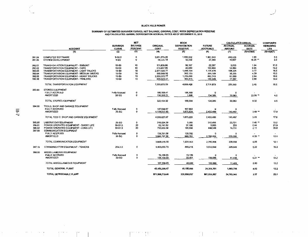
391.04 COMPUTER SOFTWARE 9-S2.5 0 3,651,575.26 1,690.032 1,961.543 288.228 7.89 6.8 391,05 SYSTEM DEVELOPMENT 5-SQ 0 59,725.18 32,332 27,393 10,957 18.35 - 2.5
392.01 TRANSPORTATION EQUIPMENT - SUBUNIT 13-SO 10 131,626.96 96,167 22297 2.033 1.54 11.0 392.02 TRANSPORTATION EQUIPMENT- CARS 13-SO 10 215,057.80 40,669 152,883 14,960 6.96 10.2 392.03 TRANSPORTATION EQUIPMENT - LIGHT TRUCKS 13-SO 10 2.871.325.77 1.448.754 1,135,439 108,226 3.77 10,5 392.04 TRANSPORTATION EQUIPMENT - MEDIUM TRUCKS 13-SO 10 803,668.92 362,133 361,169 35.265 4.39 10.2 392.05 TRANSPORTATION EQUIPMENT- HEAVY TRUCKS 13.SO 10 2,853,372.77 1,705,290 862,745 81.089 2.84 10.6 392.06 TRANSPORTATION EQUIPMENT - TRAILERS 13.SO 10 628623.37 383,415 182,346 17.587 2.80 10.4
TOTAL TRANSPORT AT/ON EQUIPMENT 7 ,503,675.59 4,036,428 2.716,879 259,160 3.45 10.5
393.00 STORES EQUIPMENT FULLY ACCRUED FuHy Accrued 0 18£,168.41 186,168 0 0 AMORTIZED 20-SQ 0 136,266.21 1,666 134.380 30,063 22.06 .. 4.5
TOTAL STORES EQUIPMENT 322.434.62 188,054 134.380 30.063 9.32 4.5
394.00 TOOLS, SHOP AND GARAGE EQUIPMENT FULLY ACCRUED Fully Accrued 0 197,599.87 197,600 0 0
T AMORTIZED 25-SQ 0 4,109,027.60 1.675.628 2 433,400 143,467 3.49 ... 17.0
-J TOTAL TOOLS. SHOP AND GARAGE EQUIPMENT 4.306,627.67 1.873.228 2,433,400 143,467 303 17.0
395.00 LABORATORY EQUIPMENT 25-SQ 0 318,024.39 5.569 312.455 23,721 7.46 - 13.2 396.01 POWER OPERATED EQUIPMENT - SHORT L!FE 30-St.5 20 52,741.62 37.100 5,093 233 0.44 21.9 396.02 POWER OPERATED EQUIPMENT - LONG UFE 30-51.5 20 792,630.34 185,556 448,548 16,731 2.11 26.8 397.00 COMMUNICATION EQUIPMENT
FULLY ACCRUED Fully Accrued 0 139,781.96 139,782 0 0 AMORTIZED 20-SQ 0 3,666,737.20 860781 2.785.956 229,558 6.26 - 12.1
TOTAL COMMUNICATION EQUIPMENT 3,806,519.18 1,020,563 2,765,956 229,558 6.03 12.1
397.10 COMMUNICATION EQUIPMENT-TOWERS 20-l1.S 0 4,403,055.70 890,216 3,512.840 229,649 5.22 15.3
398.00 MISCELLANEOUS EQUIPMENT FULLY ACCRUED Fully Accrued 0 13,139.05 13.139 0 0 AMORTIZED 20-SO 0 184,159.00 33,461 150,698 11,438 6.21 - 13.2
TOTAL MISCELLANEOUS EQUIPMENT 197 298.05 46,600 150.698 11,438 5.80 13.2
TOTAL GENERAL PLANT 43,150,288.47 19,155,066 24,354,701 1,993,726 462 12.2
TOTAL DEPRECIABLE PLANT 971,998,719.46 335,958,837 801,834,897 34,703,945 3.57 23.1
I I I , ,

310.01 340.01 350.01 350.02 360.01 36{).02 389.01
00
BLACK HILLS POWER
SUMMARY OF ESTIMATED SUR\1VOR CURVES, NET SALVAGE, ORIGINAL COST, BOOK DEPRECIATION RESERVE AND CALCULATED J:INNUAL DEPRECIATION ACCRUAL RATES AS OF DECEMBER 31, 2012
NET
SURVIVOR SALVAGE ACCOUNT CURVE PERCENT
(1) (2) (3)
NONDEPRECIABLE PU.NT
LAND LAND LAND LAND RIGHTS/RIGHTS OF WAY· NONDEPRECIABLE LAND LAND R1GHTSIRIGHTS OF WAY - NONDEPRECIABLE LAND
TOTAL NONDEPREctABLE PLANT
TOTAL ELECTRIC PLANT
• LIFE SPAN PROCEDURE USED. CURVE SHOWN IS INTERIM SURVIVOR CURVE
.... ADDITIONS AS OF JANUARY 1. 2013 WILL UTILIZE THE STANDARD AMORTIZATION RATE
NOTE· RATES FOR THE CHEYENNE PRAIRIE COMBINED CYCLE UNIT AREAS FOtlOWS: ACCOUNT BtJf
341.00 3.08 342.00 3.30 344.00 3.29 345.00 346.00
COMPOSITE
3.27 3.80 3.29
'i'
BOOK ORIGINAL DEPRECIATION FUTURE
COST RESERVE ACCRUALS (4) (5) (6)
333,639.32 31,963 2,705.00
1,053,181.88 4,692.747.84
956.864.59 (21 .. 473) 1.1ss,3n.52 (21,552)
856,913.03
9,034,429.18 (11,062)
981,033,148.64 335,947,ns 801,1!_34.897
CALCULATED ANNUAL COMPOSITE ACCRUAL ACCRUAL REMAINING AMOUNT RATE LIFE
(7) (8)=(7)/(4} (9)=(6}1(7)
34,703,945