rational functions - university of alaska systemrfrith.uaa.alaska.edu/algebra/chapter4/ch4.pdf ·...
TRANSCRIPT
Chapter 4
Rational Functions
4.1 Introduction to Rational Functions
If we add, subtract or multiply polynomial functions according to the function arithmetic rulesdefined in Section 1.5, we will produce another polynomial function. If, on the other hand, wedivide two polynomial functions, the result may not be a polynomial. In this chapter we studyrational functions - functions which are ratios of polynomials.
Definition 4.1. A rational function is a function which is the ratio of polynomial functions.Said differently, r is a rational function if it is of the form
r(x) =p(x)
q(x),
where p and q are polynomial functions.a
aAccording to this definition, all polynomial functions are also rational functions. (Take q(x) = 1).
As we recall from Section 1.4, we have domain issues anytime the denominator of a fraction iszero. In the example below, we review this concept as well as some of the arithmetic of rationalexpressions.
Example 4.1.1. Find the domain of the following rational functions. Write them in the form p(x)q(x)
for polynomial functions p and q and simplify.
1. f(x) =2x− 1
x+ 12. g(x) = 2− 3
x+ 1
3. h(x) =2x2 − 1
x2 − 1− 3x− 2
x2 − 14. r(x) =
2x2 − 1
x2 − 1÷ 3x− 2
x2 − 1
Solution.
1. To find the domain of f , we proceed as we did in Section 1.4: we find the zeros of thedenominator and exclude them from the domain. Setting x+1 = 0 results in x = −1. Hence,

302 Rational Functions
our domain is (−∞,−1)∪ (−1,∞). The expression f(x) is already in the form requested andwhen we check for common factors among the numerator and denominator we find none, sowe are done.
2. Proceeding as before, we determine the domain of g by solving x+ 1 = 0. As before, we findthe domain of g is (−∞,−1) ∪ (−1,∞). To write g(x) in the form requested, we need to geta common denominator
g(x) = 2− 3
x+ 1=
2
1− 3
x+ 1=
(2)(x+ 1)
(1)(x+ 1)− 3
x+ 1
=(2x+ 2)− 3
x+ 1=
2x− 1
x+ 1
This formula is now completely simplified.
3. The denominators in the formula for h(x) are both x2 − 1 whose zeros are x = ±1. As aresult, the domain of h is (−∞,−1) ∪ (−1, 1) ∪ (1,∞). We now proceed to simplify h(x).Since we have the same denominator in both terms, we subtract the numerators. We thenfactor the resulting numerator and denominator, and cancel out the common factor.
h(x) =2x2 − 1
x2 − 1− 3x− 2
x2 − 1=
(2x2 − 1
)− (3x− 2)
x2 − 1
=2x2 − 1− 3x+ 2
x2 − 1=
2x2 − 3x+ 1
x2 − 1
=(2x− 1)(x− 1)
(x+ 1)(x− 1)=
(2x− 1)����(x− 1)
(x+ 1)����(x− 1)
=2x− 1
x+ 1
4. To find the domain of r, it may help to temporarily rewrite r(x) as
r(x) =
2x2 − 1
x2 − 13x− 2
x2 − 1
We need to set all of the denominators equal to zero which means we need to solve not onlyx2 − 1 = 0, but also 3x−2
x2−1= 0. We find x = ±1 for the former and x = 2
3 for the latter. Our
domain is (−∞,−1)∪ (−1, 23)∪ (23 , 1
)∪ (1,∞). We simplify r(x) by rewriting the division asmultiplication by the reciprocal and then by canceling the common factor
4.1 Introduction to Rational Functions 303
r(x) =2x2 − 1
x2 − 1÷ 3x− 2
x2 − 1=
2x2 − 1
x2 − 1· x
2 − 1
3x− 2=
(2x2 − 1
) (x2 − 1
)(x2 − 1) (3x− 2)
=
(2x2 − 1
)�����(x2 − 1
)�����(x2 − 1
)(3x− 2)
=2x2 − 1
3x− 2
A few remarks about Example 4.1.1 are in order. Note that the expressions for f(x), g(x) andh(x) work out to be the same. However, only two of these functions are actually equal. Recall thatfunctions are ultimately sets of ordered pairs,1 so for two functions to be equal, they need, amongother things, to have the same domain. Since f(x) = g(x) and f and g have the same domain, theyare equal functions. Even though the formula h(x) is the same as f(x), the domain of h is differentthan the domain of f , and thus they are different functions.
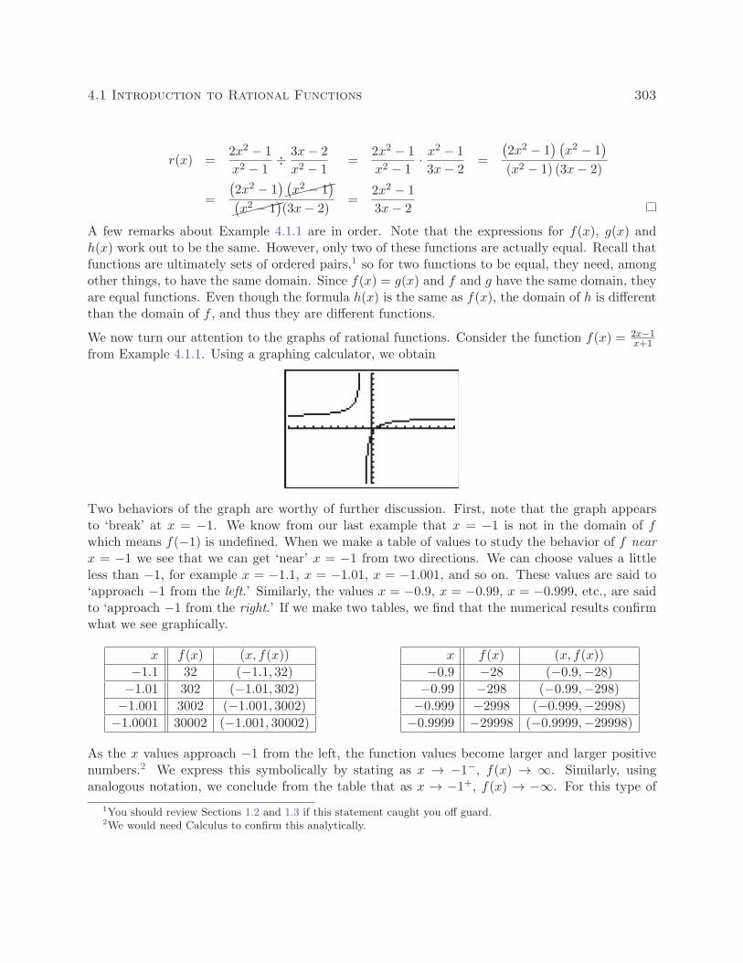
We now turn our attention to the graphs of rational functions. Consider the function f(x) = 2x−1x+1
from Example 4.1.1. Using a graphing calculator, we obtain
Two behaviors of the graph are worthy of further discussion. First, note that the graph appearsto ‘break’ at x = −1. We know from our last example that x = −1 is not in the domain of fwhich means f(−1) is undefined. When we make a table of values to study the behavior of f nearx = −1 we see that we can get ‘near’ x = −1 from two directions. We can choose values a littleless than −1, for example x = −1.1, x = −1.01, x = −1.001, and so on. These values are said to‘approach −1 from the left.’ Similarly, the values x = −0.9, x = −0.99, x = −0.999, etc., are saidto ‘approach −1 from the right.’ If we make two tables, we find that the numerical results confirmwhat we see graphically.
x f(x) (x, f(x))
−1.1 32 (−1.1, 32)−1.01 302 (−1.01, 302)−1.001 3002 (−1.001, 3002)−1.0001 30002 (−1.001, 30002)
x f(x) (x, f(x))
−0.9 −28 (−0.9,−28)−0.99 −298 (−0.99,−298)−0.999 −2998 (−0.999,−2998)−0.9999 −29998 (−0.9999,−29998)
As the x values approach −1 from the left, the function values become larger and larger positivenumbers.2 We express this symbolically by stating as x → −1−, f(x) → ∞. Similarly, usinganalogous notation, we conclude from the table that as x → −1+, f(x) → −∞. For this type of
1You should review Sections 1.2 and 1.3 if this statement caught you off guard.2We would need Calculus to confirm this analytically.

304 Rational Functions
unbounded behavior, we say the graph of y = f(x) has a vertical asymptote of x = −1. Roughlyspeaking, this means that near x = −1, the graph looks very much like the vertical line x = −1.The other feature worthy of note about the graph of y = f(x) is that it seems to ‘level off’ on theleft and right hand sides of the screen. This is a statement about the end behavior of the function.As we discussed in Section 3.1, the end behavior of a function is its behavior as x attains larger3 andlarger negative values without bound, x → −∞, and as x becomes large without bound, x → ∞.Making tables of values, we find
x f(x) (x, f(x))
−10 ≈ 2.3333 ≈ (−10, 2.3333)−100 ≈ 2.0303 ≈ (−100, 2.0303)−1000 ≈ 2.0030 ≈ (−1000, 2.0030)−10000 ≈ 2.0003 ≈ (−10000, 2.0003)
x f(x) (x, f(x))
10 ≈ 1.7273 ≈ (10, 1.7273)
100 ≈ 1.9703 ≈ (100, 1.9703)
1000 ≈ 1.9970 ≈ (1000, 1.9970)
10000 ≈ 1.9997 ≈ (10000, 1.9997)
From the tables, we see that as x → −∞, f(x) → 2+ and as x → ∞, f(x) → 2−. Here the ‘+’means ‘from above’ and the ‘−’ means ‘from below’. In this case, we say the graph of y = f(x) hasa horizontal asymptote of y = 2. This means that the end behavior of f resembles the horizontalline y = 2, which explains the ‘leveling off’ behavior we see in the calculator’s graph. We formalizethe concepts of vertical and horizontal asymptotes in the following definitions.
Definition 4.2. The line x = c is called a vertical asymptote of the graph of a functiony = f(x) if as x→ c− or as x→ c+, either f(x)→∞ or f(x)→ −∞.
Definition 4.3. The line y = c is called a horizontal asymptote of the graph of a functiony = f(x) if as x→ −∞ or as x→∞, f(x)→ c.
Note that in Definition 4.3, we write f(x) → c (not f(x) → c+ or f(x) → c−) because we areunconcerned from which direction the values f(x) approach the value c, just as long as they do so.4
In our discussion following Example 4.1.1, we determined that, despite the fact that the formula forh(x) reduced to the same formula as f(x), the functions f and h are different, since x = 1 is in the
domain of f , but x = 1 is not in the domain of h. If we graph h(x) = 2x2−1x2−1
− 3x−2x2−1
using a graphingcalculator, we are surprised to find that the graph looks identical to the graph of y = f(x). Thereis a vertical asymptote at x = −1, but near x = 1, everything seem fine. Tables of values providenumerical evidence which supports the graphical observation.
3Here, the word ‘larger’ means larger in absolute value.4As we shall see in the next section, the graphs of rational functions may, in fact, cross their horizontal asymptotes.
If this happens, however, it does so only a finite number of times, and so for each choice of x → −∞ and x → ∞,f(x) will approach c from either below (in the case f(x)→ c−) or above (in the case f(x)→ c+.) We leave f(x)→ cgeneric in our definition, however, to allow this concept to apply to less tame specimens in the Precalculus zoo, suchas Exercise 50 in Section 10.5.

4.1 Introduction to Rational Functions 305
x h(x) (x, h(x))
0.9 ≈ 0.4210 ≈ (0.9, 0.4210)
0.99 ≈ 0.4925 ≈ (0.99, 0.4925)
0.999 ≈ 0.4992 ≈ (0.999, 0.4992)
0.9999 ≈ 0.4999 ≈ (0.9999, 0.4999)
x h(x) (x, h(x))
1.1 ≈ 0.5714 ≈ (1.1, 0.5714)
1.01 ≈ 0.5075 ≈ (1.01, 0.5075)
1.001 ≈ 0.5007 ≈ (1.001, 0.5007)
1.0001 ≈ 0.5001 ≈ (1.0001, 0.5001)
We see that as x → 1−, h(x) → 0.5− and as x → 1+, h(x) → 0.5+. In other words, the points onthe graph of y = h(x) are approaching (1, 0.5), but since x = 1 is not in the domain of h, it wouldbe inaccurate to fill in a point at (1, 0.5). As we’ve done in past sections when something like thisoccurs,5 we put an open circle (also called a hole in this case6) at (1, 0.5). Below is a detailedgraph of y = h(x), with the vertical and horizontal asymptotes as dashed lines.
x
y
−4 −3 −2 1 2 3 4−1
−2
−3
−4
−5
−6
1
3
4
5
6
7
8
Neither x = −1 nor x = 1 are in the domain of h, yet the behavior of the graph of y = h(x) isdrastically different near these x-values. The reason for this lies in the second to last step whenwe simplified the formula for h(x) in Example 4.1.1, where we had h(x) = (2x−1)(x−1)
(x+1)(x−1) . The reason
x = −1 is not in the domain of h is because the factor (x + 1) appears in the denominator ofh(x); similarly, x = 1 is not in the domain of h because of the factor (x − 1) in the denominatorof h(x). The major difference between these two factors is that (x − 1) cancels with a factor inthe numerator whereas (x + 1) does not. Loosely speaking, the trouble caused by (x − 1) in thedenominator is canceled away while the factor (x + 1) remains to cause mischief. This is why thegraph of y = h(x) has a vertical asymptote at x = −1 but only a hole at x = 1. These observationsare generalized and summarized in the theorem below, whose proof is found in Calculus.
5For instance, graphing piecewise defined functions in Section 1.6.6In Calculus, we will see how these ‘holes’ can be ‘plugged’ when embarking on a more advanced study of continuity.

306 Rational Functions
Theorem 4.1. Location of Vertical Asymptotes and Holes:a Suppose r is a rationalfunction which can be written as r(x) = p(x)
q(x) where p and q have no common zeros.b Let c be areal number which is not in the domain of r.
� If q(c) �= 0, then the graph of y = r(x) has a hole at(c, p(c)q(c)
).
� If q(c) = 0, then the line x = c is a vertical asymptote of the graph of y = r(x).
aOr, ‘How to tell your asymptote from a hole in the graph.’bIn other words, r(x) is in lowest terms.
In English, Theorem 4.1 says that if x = c is not in the domain of r but, when we simplify r(x), itno longer makes the denominator 0, then we have a hole at x = c. Otherwise, the line x = c is avertical asymptote of the graph of y = r(x).
Example 4.1.2. Find the vertical asymptotes of, and/or holes in, the graphs of the followingrational functions. Verify your answers using a graphing calculator, and describe the behavior ofthe graph near them using proper notation.
1. f(x) =2x
x2 − 3 2. g(x) =x2 − x− 6
x2 − 9
3. h(x) =x2 − x− 6
x2 + 94. r(x) =
x2 − x− 6
x2 + 4x+ 4
Solution.
1. To use Theorem 4.1, we first find all of the real numbers which aren’t in the domain of f . Todo so, we solve x2 − 3 = 0 and get x = ±√3. Since the expression f(x) is in lowest terms,there is no cancellation possible, and we conclude that the lines x = −√3 and x =
√3 are
vertical asymptotes to the graph of y = f(x). The calculator verifies this claim, and from the
graph, we see that as x → −√3−, f(x) → −∞, as x → −√3
+, f(x) → ∞, as x → √
3−,
f(x)→ −∞, and finally as x→ √3+, f(x)→∞.
2. Solving x2 − 9 = 0 gives x = ±3. In lowest terms g(x) = x2−x−6x2−9
= (x−3)(x+2)(x−3)(x+3) = x+2
x+3 . Sincex = −3 continues to make trouble in the denominator, we know the line x = −3 is a verticalasymptote of the graph of y = g(x). Since x = 3 no longer produces a 0 in the denominator,we have a hole at x = 3. To find the y-coordinate of the hole, we substitute x = 3 into x+2
x+3
and find the hole is at(3, 56
). When we graph y = g(x) using a calculator, we clearly see the
vertical asymptote at x = −3, but everything seems calm near x = 3. Hence, as x → −3−,g(x)→∞, as x→ −3+, g(x)→ −∞, as x→ 3−, g(x)→ 5
6
−, and as x→ 3+, g(x)→ 5
6
+.

4.1 Introduction to Rational Functions 307
The graph of y = f(x) The graph of y = g(x)
3. The domain of h is all real numbers, since x2 + 9 = 0 has no real solutions. Accordingly, thegraph of y = h(x) is devoid of both vertical asymptotes and holes.
4. Setting x2 + 4x + 4 = 0 gives us x = −2 as the only real number of concern. Simplifying,we see r(x) = x2−x−6
x2+4x+4= (x−3)(x+2)
(x+2)2= x−3
x+2 . Since x = −2 continues to produce a 0 in the
denominator of the reduced function, we know x = −2 is a vertical asymptote to the graph.The calculator bears this out, and, moreover, we see that as x → −2−, r(x) → ∞ and asx→ −2+, r(x)→ −∞.
The graph of y = h(x) The graph of y = r(x)
Our next example gives us a physical interpretation of a vertical asymptote. This type of modelarises from a family of equations cheerily named ‘doomsday’ equations.7
Example 4.1.3. A mathematical model for the population P , in thousands, of a certain speciesof bacteria, t days after it is introduced to an environment is given by P (t) = 100
(5−t)2, 0 ≤ t < 5.
1. Find and interpret P (0).
2. When will the population reach 100,000?
3. Determine the behavior of P as t → 5−. Interpret this result graphically and within thecontext of the problem.
7These functions arise in Differential Equations. The unfortunate name will make sense shortly.

308 Rational Functions
Solution.
1. Substituting t = 0 gives P (0) = 100(5−0)2
= 4, which means 4000 bacteria are initially introduced
into the environment.
2. To find when the population reaches 100,000, we first need to remember that P (t) is measuredin thousands. In other words, 100,000 bacteria corresponds to P (t) = 100. Substituting forP (t) gives the equation 100
(5−t)2= 100. Clearing denominators and dividing by 100 gives
(5 − t)2 = 1, which, after extracting square roots, produces t = 4 or t = 6. Of these twosolutions, only t = 4 in our domain, so this is the solution we keep. Hence, it takes 4 days forthe population of bacteria to reach 100,000.
3. To determine the behavior of P as t→ 5−, we can make a table
t P (t)
4.9 10000
4.99 1000000
4.999 100000000
4.9999 10000000000
In other words, as t → 5−, P (t) → ∞. Graphically, the line t = 5 is a vertical asymptote ofthe graph of y = P (t). Physically, this means that the population of bacteria is increasingwithout bound as we near 5 days, which cannot actually happen. For this reason, t = 5 iscalled the ‘doomsday’ for this population. There is no way any environment can supportinfinitely many bacteria, so shortly before t = 5 the environment would collapse.
Now that we have thoroughly investigated vertical asymptotes, we can turn our attention to hori-zontal asymptotes. The next theorem tells us when to expect horizontal asymptotes.
Theorem 4.2. Location of Horizontal Asymptotes: Suppose r is a rational function andr(x) = p(x)
q(x) , where p and q are polynomial functions with leading coefficients a and b, respectively.
� If the degree of p(x) is the same as the degree of q(x), then y = ab is thea horizontal
asymptote of the graph of y = r(x).
� If the degree of p(x) is less than the degree of q(x), then y = 0 is the horizontal asymptoteof the graph of y = r(x).
� If the degree of p(x) is greater than the degree of q(x), then the graph of y = r(x) has nohorizontal asymptotes.
aThe use of the definite article will be justified momentarily.
Like Theorem 4.1, Theorem 4.2 is proved using Calculus. Nevertheless, we can understand the ideabehind it using our example f(x) = 2x−1
x+1 . If we interpret f(x) as a division problem, (2x−1)÷(x+1),

4.1 Introduction to Rational Functions 309
we find that the quotient is 2 with a remainder of −3. Using what we know about polynomialdivision, specifically Theorem 3.4, we get 2x − 1 = 2(x + 1) − 3. Dividing both sides by (x + 1)gives 2x−1
x+1 = 2 − 3x+1 . (You may remember this as the formula for g(x) in Example 4.1.1.) As x
becomes unbounded in either direction, the quantity 3x+1 gets closer and closer to 0 so that the
values of f(x) become closer and closer8 to 2. In symbols, as x→ ±∞, f(x)→ 2, and we have theresult.9 Notice that the graph gets close to the same y value as x → −∞ or x → ∞. This meansthat the graph can have only one horizontal asymptote if it is going to have one at all. Thus wewere justified in using ‘the’ in the previous theorem.
Alternatively, we can use what we know about end behavior of polynomials to help us understandthis theorem. From Theorem 3.2, we know the end behavior of a polynomial is determined by itsleading term. Applying this to the numerator and denominator of f(x), we get that as x → ±∞,f(x) = 2x−1
x+1 ≈ 2xx = 2. This last approach is useful in Calculus, and, indeed, is made rigorous there.
(Keep this in mind for the remainder of this paragraph.) Applying this reasoning to the general
case, suppose r(x) = p(x)q(x) where a is the leading coefficient of p(x) and b is the leading coefficient
of q(x). As x → ±∞, r(x) ≈ axn
bxm , where n and m are the degrees of p(x) and q(x), respectively.If the degree of p(x) and the degree of q(x) are the same, then n = m so that r(x) ≈ a
b , whichmeans y = a
b is the horizontal asymptote in this case. If the degree of p(x) is less than the degreeof q(x), then n < m, so m− n is a positive number, and hence, r(x) ≈ a
bxm−n → 0 as x→ ±∞. Ifthe degree of p(x) is greater than the degree of q(x), then n > m, and hence n −m is a positive
number and r(x) ≈ axn−m
b , which becomes unbounded as x→ ±∞. As we said before, if a rationalfunction has a horizontal asymptote, then it will have only one. (This is not true for other typesof functions we shall see in later chapters.)
Example 4.1.4. List the horizontal asymptotes, if any, of the graphs of the following functions.Verify your answers using a graphing calculator, and describe the behavior of the graph near themusing proper notation.
1. f(x) =5x
x2 + 1 2. g(x) =x2 − 4
x+ 13. h(x) =
6x3 − 3x+ 1
5− 2x3
Solution.
1. The numerator of f(x) is 5x, which has degree 1. The denominator of f(x) is x2 + 1, whichhas degree 2. Applying Theorem 4.2, y = 0 is the horizontal asymptote. Sure enough, we seefrom the graph that as x→ −∞, f(x)→ 0− and as x→∞, f(x)→ 0+.
2. The numerator of g(x), x2 − 4, has degree 2, but the degree of the denominator, x + 1, hasdegree 1. By Theorem 4.2, there is no horizontal asymptote. From the graph, we see thatthe graph of y = g(x) doesn’t appear to level off to a constant value, so there is no horizontalasymptote.10
8As seen in the tables immediately preceding Definition 4.2.9More specifically, as x→ −∞, f(x)→ 2+, and as x→∞, f(x)→ 2−.
10Sit tight! We’ll revisit this function and its end behavior shortly.

310 Rational Functions
3. The degrees of the numerator and denominator of h(x) are both three, so Theorem 4.2 tellsus y = 6
−2 = −3 is the horizontal asymptote. We see from the calculator’s graph that asx→ −∞, h(x)→ −3+, and as x→∞, h(x)→ −3−.
The graph of y = f(x) The graph of y = g(x) The graph of y = h(x)
Our next example of the section gives us a real-world application of a horizontal asymptote.11
Example 4.1.5. The number of students N at local college who have had the flu t months afterthe semester begins can be modeled by the formula N(t) = 500− 450
1+3t for t ≥ 0.
1. Find and interpret N(0).
2. How long will it take until 300 students will have had the flu?
3. Determine the behavior of N as t → ∞. Interpret this result graphically and within thecontext of the problem.
Solution.
1. N(0) = 500 − 4501+3(0) = 50. This means that at the beginning of the semester, 50 students
have had the flu.
2. We set N(t) = 300 to get 500− 4501+3t = 300 and solve. Isolating the fraction gives 450
1+3t = 200.
Clearing denominators gives 450 = 200(1 + 3t). Finally, we get t = 512 . This means it will
take 512 months, or about 13 days, for 300 students to have had the flu.
3. To determine the behavior of N as t→∞, we can use a table.
t N(t)
10 ≈ 485.48
100 ≈ 498.50
1000 ≈ 499.85
10000 ≈ 499.98
The table suggests that as t → ∞, N(t) → 500. (More specifically, 500−.) This means astime goes by, only a total of 500 students will have ever had the flu.
11Though the population below is more accurately modeled with the functions in Chapter 6, we approximate it(using Calculus, of course!) using a rational function.

4.1 Introduction to Rational Functions 311
We close this section with a discussion of the third (and final!) kind of asymptote which can be
associated with the graphs of rational functions. Let us return to the function g(x) = x2−4x+1 in
Example 4.1.4. Performing long division,12 we get g(x) = x2−4x+1 = x − 1 − 3
x+1 . Since the term3
x+1 → 0 as x → ±∞, it stands to reason that as x becomes unbounded, the function values
g(x) = x− 1− 3x+1 ≈ x− 1. Geometrically, this means that the graph of y = g(x) should resemble
the line y = x− 1 as x→ ±∞. We see this play out both numerically and graphically below.
x g(x) x− 1
−10 ≈ −10.6667 −11−100 ≈ −100.9697 −101−1000 ≈ −1000.9970 −1001−10000 ≈ −10000.9997 −10001
x g(x) x− 1
10 ≈ 8.7273 9
100 ≈ 98.9703 99
1000 ≈ 998.9970 999
10000 ≈ 9998.9997 9999
y = g(x) and y = x− 1 y = g(x) and y = x− 1as x→ −∞ as x→∞
The way we symbolize the relationship between the end behavior of y = g(x) with that of the liney = x − 1 is to write ‘as x → ±∞, g(x) → x − 1.’ In this case, we say the line y = x − 1 is aslant asymptote13 to the graph of y = g(x). Informally, the graph of a rational function has aslant asymptote if, as x → ∞ or as x → −∞, the graph resembles a non-horizontal, or ‘slanted’line. Formally, we define a slant asymptote as follows.
Definition 4.4. The line y = mx + b where m �= 0 is called a slant asymptote of the graphof a function y = f(x) if as x→ −∞ or as x→∞, f(x)→ mx+ b.
A few remarks are in order. First, note that the stipulation m �= 0 in Definition 4.4 is whatmakes the ‘slant’ asymptote ‘slanted’ as opposed to the case when m = 0 in which case we’d have ahorizontal asymptote. Secondly, while we have motivated what me mean intuitively by the notation‘f(x)→ mx+b,’ like so many ideas in this section, the formal definition requires Calculus. Anotherway to express this sentiment, however, is to rephrase ‘f(x) → mx + b’ as ‘f(x) − (mx + b) → 0.’In other words, the graph of y = f(x) has the slant asymptote y = mx+ b if and only if the graphof y = f(x)− (mx+ b) has a horizontal asymptote y = 0.
12See the remarks following Theorem 4.2.13Also called an ‘oblique’ asymptote in some, ostensibly higher class (and more expensive), texts.

312 Rational Functions
Our next task is to determine the conditions under which the graph of a rational function hasa slant asymptote, and if it does, how to find it. In the case of g(x) = x2−4
x+1 , the degree of the
numerator x2 − 4 is 2, which is exactly one more than the degree if its denominator x + 1 whichis 1. This results in a linear quotient polynomial, and it is this quotient polynomial which is theslant asymptote. Generalizing this situation gives us the following theorem.14
Theorem 4.3. Determination of Slant Asymptotes: Suppose r is a rational function andr(x) = p(x)
q(x) , where the degree of p is exactly one more than the degree of q. Then the graph of
y = r(x) has the slant asymptote y = L(x) where L(x) is the quotient obtained by dividingp(x) by q(x).
In the same way that Theorem 4.2 gives us an easy way to see if the graph of a rational functionr(x) = p(x)
q(x) has a horizontal asymptote by comparing the degrees of the numerator and denominator,Theorem 4.3 gives us an easy way to check for slant asymptotes. Unlike Theorem 4.2, which givesus a quick way to find the horizontal asymptotes (if any exist), Theorem 4.3 gives us no such‘short-cut’. If a slant asymptote exists, we have no recourse but to use long division to find it.15
Example 4.1.6. Find the slant asymptotes of the graphs of the following functions if they exist.Verify your answers using a graphing calculator and describe the behavior of the graph near themusing proper notation.
1. f(x) =x2 − 4x+ 2
1− x2. g(x) =
x2 − 4
x− 23. h(x) =
x3 + 1
x2 − 4
Solution.
1. The degree of the numerator is 2 and the degree of the denominator is 1, so Theorem 4.3guarantees us a slant asymptote. To find it, we divide 1− x = −x + 1 into x2 − 4x + 2 andget a quotient of −x+ 3, so our slant asymptote is y = −x+ 3. We confirm this graphically,and we see that as x → −∞, the graph of y = f(x) approaches the asymptote from below,and as x→∞, the graph of y = f(x) approaches the asymptote from above.16
2. As with the previous example, the degree of the numerator g(x) = x2−4x−2 is 2 and the degree
of the denominator is 1, so Theorem 4.3 applies. In this case,
g(x) =x2 − 4
x− 2=
(x+ 2)(x− 2)
(x− 2)=
(x+ 2)����(x− 2)
����� 1(x− 2)
= x+ 2, x �= 2
14Once again, this theorem is brought to you courtesy of Theorem 3.4 and Calculus.15That’s OK, though. In the next section, we’ll use long division to analyze end behavior and it’s worth the effort!16Note that we are purposefully avoiding notation like ‘as x→∞, f(x)→ (−x+3)+. While it is possible to define
these notions formally with Calculus, it is not standard to do so. Besides, with the introduction of the symbol ‘�’ inthe next section, the authors feel we are in enough trouble already.

4.1 Introduction to Rational Functions 313
so we have that the slant asymptote y = x+ 2 is identical to the graph of y = g(x) except atx = 2 (where the latter has a ‘hole’ at (2, 4).) The calculator supports this claim.17
3. For h(x) = x3+1x2−4
, the degree of the numerator is 3 and the degree of the denominator is 2 so
again, we are guaranteed the existence of a slant asymptote. The long division(x3 + 1
) ÷(x2 − 4
)gives a quotient of just x, so our slant asymptote is the line y = x. The calculator
confirms this, and we find that as x→ −∞, the graph of y = h(x) approaches the asymptotefrom below, and as x→∞, the graph of y = h(x) approaches the asymptote from above.
The graph of y = f(x) The graph of y = g(x) The graph of y = h(x)
The reader may be a bit disappointed with the authors at this point owing to the fact that in Exam-ples 4.1.2, 4.1.4, and 4.1.6, we used the calculator to determine function behavior near asymptotes.We rectify that in the next section where we, in excruciating detail, demonstrate the usefulness of‘number sense’ to reveal this behavior analytically.
17While the word ‘asymptote’ has the connotation of ‘approaching but not equaling,’ Definitions 4.3 and 4.4 invitethe same kind of pathologies we saw with Definitions 1.11 in Section 1.6.
314 Rational Functions
4.1.1 Exercises
In Exercises 1 - 18, for the given rational function f :
� Find the domain of f .
� Identify any vertical asymptotes of the graph of y = f(x).
� Identify any holes in the graph.
� Find the horizontal asymptote, if it exists.
� Find the slant asymptote, if it exists.
� Graph the function using a graphing utility and describe the behavior near the asymptotes.
1. f(x) =x
3x− 6 2. f(x) =3 + 7x
5− 2x3. f(x) =
x
x2 + x− 12
4. f(x) =x
x2 + 1 5. f(x) =x+ 7
(x+ 3)2 6. f(x) =x3 + 1
x2 − 1
7. f(x) =4x
x2 + 48. f(x) =
4x
x2 − 4 9. f(x) =x2 − x− 12
x2 + x− 6
10. f(x) =3x2 − 5x− 2
x2 − 911. f(x) =
x3 + 2x2 + x
x2 − x− 212. f(x) =
x3 − 3x+ 1
x2 + 1
13. f(x) =2x2 + 5x− 3
3x+ 214. f(x) =
−x3 + 4x
x2 − 915. f(x) =
−5x4 − 3x3 + x2 − 10
x3 − 3x2 + 3x− 1
16. f(x) =x3
1− x17. f(x) =
18− 2x2
x2 − 918. f(x) =
x3 − 4x2 − 4x− 5
x2 + x+ 1
19. The cost C in dollars to remove p% of the invasive species of Ippizuti fish from SasquatchPond is given by
C(p) =1770p
100− p, 0 ≤ p < 100
(a) Find and interpret C(25) and C(95).
(b) What does the vertical asymptote at x = 100 mean within the context of the problem?
(c) What percentage of the Ippizuti fish can you remove for �40000?
20. In Exercise 71 in Section 1.4, the population of Sasquatch in Portage County was modeledby the function
P (t) =150t
t+ 15,
where t = 0 represents the year 1803. Find the horizontal asymptote of the graph of y = P (t)and explain what it means.

4.1 Introduction to Rational Functions 315
21. Recall from Example 1.5.3 that the cost C (in dollars) to make x dOpi media players isC(x) = 100x+ 2000, x ≥ 0.
(a) Find a formula for the average cost C(x). Recall: C(x) = C(x)x .
(b) Find and interpret C(1) and C(100).
(c) How many dOpis need to be produced so that the average cost per dOpi is $200?
(d) Interpret the behavior of C(x) as x→ 0+. (HINT: You may want to find the fixed costC(0) to help in your interpretation.)
(e) Interpret the behavior of C(x) as x → ∞. (HINT: You may want to find the variablecost (defined in Example 2.1.5 in Section 2.1) to help in your interpretation.)
22. In Exercise 35 in Section 3.1, we fit a few polynomial models to the following electric circuitdata. (The circuit was built with a variable resistor. For each of the following resistance values(measured in kilo-ohms, kΩ), the corresponding power to the load (measured in milliwatts,mW ) is given in the table below.)18
Resistance: (kΩ) 1.012 2.199 3.275 4.676 6.805 9.975
Power: (mW ) 1.063 1.496 1.610 1.613 1.505 1.314
Using some fundamental laws of circuit analysis mixed with a healthy dose of algebra, we canderive the actual formula relating power to resistance. For this circuit, it is P (x) = 25x
(x+3.9)2,
where x is the resistance value, x ≥ 0.
(a) Graph the data along with the function y = P (x) on your calculator.
(b) Use your calculator to approximate the maximum power that can be delivered to theload. What is the corresponding resistance value?
(c) Find and interpret the end behavior of P (x) as x→∞.
23. In his now famous 1919 dissertation The Learning Curve Equation, Louis Leon Thurstonepresents a rational function which models the number of words a person can type in fourminutes as a function of the number of pages of practice one has completed. (This paper,which is now in the public domain and can be found here, is from a bygone era when studentsat business schools took typing classes on manual typewriters.) Using his original notation
and original language, we have Y = L(X+P )(X+P )+R where L is the predicted practice limit in terms
of speed units, X is pages written, Y is writing speed in terms of words in four minutes, P isequivalent previous practice in terms of pages and R is the rate of learning. In Figure 5 of thepaper, he graphs a scatter plot and the curve Y = 216(X+19)
X+148 . Discuss this equation with yourclassmates. How would you update the notation? Explain what the horizontal asymptote ofthe graph means. You should take some time to look at the original paper. Skip over thecomputations you don’t understand yet and try to get a sense of the time and place in whichthe study was conducted.
18The authors wish to thank Don Anthan and Ken White of Lakeland Community College for devising this problemand generating the accompanying data set.

316 Rational Functions
4.1.2 Answers
1. f(x) =x
3x− 6Domain: (−∞, 2) ∪ (2,∞)Vertical asymptote: x = 2As x→ 2−, f(x)→ −∞As x→ 2+, f(x)→∞No holes in the graphHorizontal asymptote: y = 1
3
As x→ −∞, f(x)→ 13
−
As x→∞, f(x)→ 13
+
2. f(x) =3 + 7x
5− 2xDomain: (−∞, 52) ∪ (52 ,∞)Vertical asymptote: x = 5
2
As x→ 52
−, f(x)→∞
As x→ 52
+, f(x)→ −∞
No holes in the graphHorizontal asymptote: y = −7
2
As x→ −∞, f(x)→ −72
+
As x→∞, f(x)→ −72
−
3. f(x) =x
x2 + x− 12=
x
(x+ 4)(x− 3)Domain: (−∞,−4) ∪ (−4, 3) ∪ (3,∞)Vertical asymptotes: x = −4, x = 3As x→ −4−, f(x)→ −∞As x→ −4+, f(x)→∞As x→ 3−, f(x)→ −∞As x→ 3+, f(x)→∞No holes in the graphHorizontal asymptote: y = 0As x→ −∞, f(x)→ 0−
As x→∞, f(x)→ 0+
4. f(x) =x
x2 + 1Domain: (−∞,∞)No vertical asymptotesNo holes in the graphHorizontal asymptote: y = 0As x→ −∞, f(x)→ 0−
As x→∞, f(x)→ 0+
5. f(x) =x+ 7
(x+ 3)2
Domain: (−∞,−3) ∪ (−3,∞)Vertical asymptote: x = −3As x→ −3−, f(x)→∞As x→ −3+, f(x)→∞No holes in the graphHorizontal asymptote: y = 019As x→ −∞, f(x)→ 0−
As x→∞, f(x)→ 0+
6. f(x) =x3 + 1
x2 − 1=
x2 − x+ 1
x− 1Domain: (−∞,−1) ∪ (−1, 1) ∪ (1,∞)Vertical asymptote: x = 1As x→ 1−, f(x)→ −∞As x→ 1+, f(x)→∞Hole at (−1,−3
2)Slant asymptote: y = xAs x→ −∞, the graph is below y = xAs x→∞, the graph is above y = x
19This is hard to see on the calculator, but trust me, the graph is below the x-axis to the left of x = −7.

4.1 Introduction to Rational Functions 317
7. f(x) =4x
x2 + 4Domain: (−∞,∞)No vertical asymptotesNo holes in the graphHorizontal asymptote: y = 0As x→ −∞, f(x)→ 0−
As x→∞, f(x)→ 0+
8. f(x) =4x
x2 − 4=
4x
(x+ 2)(x− 2)Domain: (−∞,−2) ∪ (−2, 2) ∪ (2,∞)Vertical asymptotes: x = −2, x = 2As x→ −2−, f(x)→ −∞As x→ −2+, f(x)→∞As x→ 2−, f(x)→ −∞As x→ 2+, f(x)→∞No holes in the graphHorizontal asymptote: y = 0As x→ −∞, f(x)→ 0−
As x→∞, f(x)→ 0+
9. f(x) =x2 − x− 12
x2 + x− 6=
x− 4
x− 2Domain: (−∞,−3) ∪ (−3, 2) ∪ (2,∞)Vertical asymptote: x = 2As x→ 2−, f(x)→∞As x→ 2+, f(x)→ −∞Hole at
(−3, 75)Horizontal asymptote: y = 1As x→ −∞, f(x)→ 1+
As x→∞, f(x)→ 1−
10. f(x) =3x2 − 5x− 2
x2 − 9=
(3x+ 1)(x− 2)
(x+ 3)(x− 3)Domain: (−∞,−3) ∪ (−3, 3) ∪ (3,∞)Vertical asymptotes: x = −3, x = 3As x→ −3−, f(x)→∞As x→ −3+, f(x)→ −∞As x→ 3−, f(x)→ −∞As x→ 3+, f(x)→∞No holes in the graphHorizontal asymptote: y = 3As x→ −∞, f(x)→ 3+
As x→∞, f(x)→ 3−
11. f(x) =x3 + 2x2 + x
x2 − x− 2=
x(x+ 1)
x− 2Domain: (−∞,−1) ∪ (−1, 2) ∪ (2,∞)Vertical asymptote: x = 2As x→ 2−, f(x)→ −∞As x→ 2+, f(x)→∞Hole at (−1, 0)Slant asymptote: y = x+ 3As x→ −∞, the graph is below y = x+ 3As x→∞, the graph is above y = x+ 3
12. f(x) =x3 − 3x+ 1
x2 + 1Domain: (−∞,∞)No vertical asymptotesNo holes in the graphSlant asymptote: y = xAs x→ −∞, the graph is above y = xAs x→∞, the graph is below y = x

318 Rational Functions
13. f(x) =2x2 + 5x− 3
3x+ 2Domain:
(−∞,−23
) ∪ (−23 ,∞
)Vertical asymptote: x = −2
3
As x→ −23
−, f(x)→∞
As x→ −23
+, f(x)→ −∞
No holes in the graphSlant asymptote: y = 2
3x+ 119
As x→ −∞, the graph is above y = 23x+
119
As x→∞, the graph is below y = 23x+ 11
9
14. f(x) =−x3 + 4x
x2 − 9=
−x3 + 4x
(x− 3)(x+ 3)Domain: (−∞,−3) ∪ (−3, 3) ∪ (3,∞)Vertical asymptotes: x = −3, x = 3As x→ −3−, f(x)→∞As x→ −3+, f(x)→ −∞As x→ 3−, f(x)→∞As x→ 3+, f(x)→ −∞No holes in the graphSlant asymptote: y = −xAs x→ −∞, the graph is above y = −xAs x→∞, the graph is below y = −x
15. f(x) =−5x4 − 3x3 + x2 − 10
x3 − 3x2 + 3x− 1
=−5x4 − 3x3 + x2 − 10
(x− 1)3
Domain: (−∞, 1) ∪ (1,∞)Vertical asymptotes: x = 1As x→ 1−, f(x)→∞As x→ 1+, f(x)→ −∞No holes in the graphSlant asymptote: y = −5x− 18As x→ −∞, the graph is above y = −5x− 18
As x→∞, the graph is below y = −5x− 18
16. f(x) =x3
1− xDomain: (−∞, 1) ∪ (1,∞)Vertical asymptote: x = 1As x→ 1−, f(x)→∞As x→ 1+, f(x)→ −∞No holes in the graphNo horizontal or slant asymptoteAs x→ −∞, f(x)→ −∞As x→∞, f(x)→ −∞
17. f(x) =18− 2x2
x2 − 9= −2
Domain: (−∞,−3) ∪ (−3, 3) ∪ (3,∞)No vertical asymptotesHoles in the graph at (−3,−2) and (3,−2)Horizontal asymptote y = −2As x→ ±∞, f(x) = −2
18. f(x) =x3 − 4x2 − 4x− 5
x2 + x+ 1= x− 5
Domain: (−∞,∞)No vertical asymptotesNo holes in the graphSlant asymptote: y = x− 5f(x) = x− 5 everywhere.
19. (a) C(25) = 590 means it costs �590 to remove 25% of the fish and and C(95) = 33630means it would cost �33630 to remove 95% of the fish from the pond.
(b) The vertical asymptote at x = 100 means that as we try to remove 100% of the fish fromthe pond, the cost increases without bound; i.e., it’s impossible to remove all of the fish.
(c) For �40000 you could remove about 95.76% of the fish.

4.1 Introduction to Rational Functions 319
20. The horizontal asymptote of the graph of P (t) = 150tt+15 is y = 150 and it means that the model
predicts the population of Sasquatch in Portage County will never exceed 150.
21. (a) C(x) = 100x+2000x , x > 0.
(b) C(1) = 2100 and C(100) = 120. When just 1 dOpi is produced, the cost per dOpi is$2100, but when 100 dOpis are produced, the cost per dOpi is $120.
(c) C(x) = 200 when x = 20. So to get the cost per dOpi to $200, 20 dOpis need to beproduced.
(d) As x → 0+, C(x) → ∞. This means that as fewer and fewer dOpis are produced,the cost per dOpi becomes unbounded. In this situation, there is a fixed cost of $2000(C(0) = 2000), we are trying to spread that $2000 over fewer and fewer dOpis.
(e) As x→∞, C(x)→ 100+. This means that as more and more dOpis are produced, thecost per dOpi approaches $100, but is always a little more than $100. Since $100 is thevariable cost per dOpi (C(x) = 100x+2000), it means that no matter how many dOpisare produced, the average cost per dOpi will always be a bit higher than the variablecost to produce a dOpi. As before, we can attribute this to the $2000 fixed cost, whichfactors into the average cost per dOpi no matter how many dOpis are produced.
22. (a)
(b) The maximum power is approximately 1.603 mW which corresponds to 3.9 kΩ.
(c) As x → ∞, P (x) → 0+ which means as the resistance increases without bound, thepower diminishes to zero.

320 Rational Functions
4.2 Graphs of Rational Functions
In this section, we take a closer look at graphing rational functions. In Section 4.1, we learned thatthe graphs of rational functions may have holes in them and could have vertical, horizontal andslant asymptotes. Theorems 4.1, 4.2 and 4.3 tell us exactly when and where these behaviors willoccur, and if we combine these results with what we already know about graphing functions, wewill quickly be able to generate reasonable graphs of rational functions.
One of the standard tools we will use is the sign diagram which was first introduced in Section 2.4,and then revisited in Section 3.1. In those sections, we operated under the belief that a functioncouldn’t change its sign without its graph crossing through the x-axis. The major theorem weused to justify this belief was the Intermediate Value Theorem, Theorem 3.1. It turns out theIntermediate Value Theorem applies to all continuous functions,1 not just polynomials. Althoughrational functions are continuous on their domains,2 Theorem 4.1 tells us that vertical asymptotesand holes occur at the values excluded from their domains. In other words, rational functionsaren’t continuous at these excluded values which leaves open the possibility that the function couldchange sign without crossing through the x-axis. Consider the graph of y = h(x) from Example4.1.1, recorded below for convenience. We have added its x-intercept at
(12 , 0
)for the discussion
that follows. Suppose we wish to construct a sign diagram for h(x). Recall that the intervals whereh(x) > 0, or (+), correspond to the x-values where the graph of y = h(x) is above the x-axis; theintervals on which h(x) < 0, or (−) correspond to where the graph is below the x-axis.
x
y
12
−4 −3 −2 1 2 3 4
−1
−2
−3
−4
−5
−6
1
3
4
5
6
7
8
−1 12
1
(+) � (−) 0 (+) � (+)
As we examine the graph of y = h(x), reading from left to right, we note that from (−∞,−1),the graph is above the x-axis, so h(x) is (+) there. At x = −1, we have a vertical asymptote, atwhich point the graph ‘jumps’ across the x-axis. On the interval
(−1, 12), the graph is below the
1Recall that, for our purposes, this means the graphs are devoid of any breaks, jumps or holes2Another result from Calculus.

4.2 Graphs of Rational Functions 321
x-axis, so h(x) is (−) there. The graph crosses through the x-axis at(12 , 0
)and remains above
the x-axis until x = 1, where we have a ‘hole’ in the graph. Since h(1) is undefined, there is nosign here. So we have h(x) as (+) on the interval
(12 , 1
). Continuing, we see that on (1,∞), the
graph of y = h(x) is above the x-axis, so we mark (+) there. To construct a sign diagram fromthis information, we not only need to denote the zero of h, but also the places not in the domain ofh. As is our custom, we write ‘0’ above 1
2 on the sign diagram to remind us that it is a zero of h.We need a different notation for −1 and 1, and we have chosen to use ‘�’ - a nonstandard symbolcalled the interrobang. We use this symbol to convey a sense of surprise, caution and wonderment- an appropriate attitude to take when approaching these points. The moral of the story is thatwhen constructing sign diagrams for rational functions, we include the zeros as well as the valuesexcluded from the domain.
Steps for Constructing a Sign Diagram for a Rational Function
Suppose r is a rational function.
1. Place any values excluded from the domain of r on the number line with an ‘�’ above them.
2. Find the zeros of r and place them on the number line with the number 0 above them.
3. Choose a test value in each of the intervals determined in steps 1 and 2.
4. Determine the sign of r(x) for each test value in step 3, and write that sign above thecorresponding interval.
We now present our procedure for graphing rational functions and apply it to a few exhaustiveexamples. Please note that we decrease the amount of detail given in the explanations as we movethrough the examples. The reader should be able to fill in any details in those steps which we haveabbreviated.
Steps for Graphing Rational Functions
Suppose r is a rational function.
1. Find the domain of r.
2. Reduce r(x) to lowest terms, if applicable.
3. Find the x- and y-intercepts of the graph of y = r(x), if they exist.
4. Determine the location of any vertical asymptotes or holes in the graph, if they exist.Analyze the behavior of r on either side of the vertical asymptotes, if applicable.
5. Analyze the end behavior of r. Find the horizontal or slant asymptote, if one exists.
6. Use a sign diagram and plot additional points, as needed, to sketch the graph of y = r(x).
322 Rational Functions
Example 4.2.1. Sketch a detailed graph of f(x) =3x
x2 − 4.
Solution. We follow the six step procedure outlined above.
1. As usual, we set the denominator equal to zero to get x2 − 4 = 0. We find x = ±2, so ourdomain is (−∞,−2) ∪ (−2, 2) ∪ (2,∞).
2. To reduce f(x) to lowest terms, we factor the numerator and denominator which yieldsf(x) = 3x
(x−2)(x+2) . There are no common factors which means f(x) is already in lowestterms.
3. To find the x-intercepts of the graph of y = f(x), we set y = f(x) = 0. Solving 3x(x−2)(x+2) = 0
results in x = 0. Since x = 0 is in our domain, (0, 0) is the x-intercept. To find the y-intercept,we set x = 0 and find y = f(0) = 0, so that (0, 0) is our y-intercept as well.3
4. The two numbers excluded from the domain of f are x = −2 and x = 2. Since f(x) didn’treduce at all, both of these values of x still cause trouble in the denominator. Thus byTheorem 4.1, x = −2 and x = 2 are vertical asymptotes of the graph. We can actually goa step further at this point and determine exactly how the graph approaches the asymptotenear each of these values. Though not absolutely necessary,4 it is good practice for thoseheading off to Calculus. For the discussion that follows, it is best to use the factored form off(x) = 3x
(x−2)(x+2) .
� The behavior of y = f(x) as x→ −2: Suppose x→ −2−. If we were to build a table ofvalues, we’d use x-values a little less than −2, say −2.1, −2.01 and −2.001. While thereis no harm in actually building a table like we did in Section 4.1, we want to develop a‘number sense’ here. Let’s think about each factor in the formula of f(x) as we imaginesubstituting a number like x = −2.000001 into f(x). The quantity 3x would be veryclose to −6, the quantity (x−2) would be very close to −4, and the factor (x+2) wouldbe very close to 0. More specifically, (x + 2) would be a little less than 0, in this case,−0.000001. We will call such a number a ‘very small (−)’, ‘very small’ meaning close tozero in absolute value. So, mentally, as x→ −2−, we estimate
f(x) =3x
(x− 2)(x+ 2)≈ −6
(−4) (very small (−)) =3
2 (very small (−))Now, the closer x gets to −2, the smaller (x + 2) will become, so even though we aremultiplying our ‘very small (−)’ by 2, the denominator will continue to get smaller andsmaller, and remain negative. The result is a fraction whose numerator is positive, butwhose denominator is very small and negative. Mentally,
f(x) ≈ 3
2 (very small (−)) ≈3
very small (−) ≈ very big (−)3As we mentioned at least once earlier, since functions can have at most one y-intercept, once we find that (0, 0)
is on the graph, we know it is the y-intercept.4The sign diagram in step 6 will also determine the behavior near the vertical asymptotes.

4.2 Graphs of Rational Functions 323
The term ‘very big (−)’ means a number with a large absolute value which is negative.5
What all of this means is that as x → −2−, f(x) → −∞. Now suppose we wanted todetermine the behavior of f(x) as x → −2+. If we imagine substituting something alittle larger than −2 in for x, say −1.999999, we mentally estimate
f(x) ≈ −6(−4) (very small (+))
=3
2 (very small (+))≈ 3
very small (+)≈ very big (+)
We conclude that as x→ −2+, f(x)→∞.
� The behavior of y = f(x) as x → 2: Consider x → 2−. We imagine substitutingx = 1.999999. Approximating f(x) as we did above, we get
f(x) ≈ 6
(very small (−)) (4) =3
2 (very small (−)) ≈3
very small (−) ≈ very big (−)
We conclude that as x→ 2−, f(x)→ −∞. Similarly, as x→ 2+, we imagine substitutingx = 2.000001 to get f(x) ≈ 3
very small (+) ≈ very big (+). So as x→ 2+, f(x)→∞.
Graphically, we have that near x = −2 and x = 2 the graph of y = f(x) looks like6
x
y
−3 −1 1 3
5. Next, we determine the end behavior of the graph of y = f(x). Since the degree of thenumerator is 1, and the degree of the denominator is 2, Theorem 4.2 tells us that y = 0is the horizontal asymptote. As with the vertical asymptotes, we can glean more detailedinformation using ‘number sense’. For the discussion below, we use the formula f(x) = 3x
x2−4.
� The behavior of y = f(x) as x → −∞: If we were to make a table of values to discussthe behavior of f as x→ −∞, we would substitute very ‘large’ negative numbers in forx, say for example, x = −1 billion. The numerator 3x would then be −3 billion, whereas
5The actual retail value of f(−2.000001) is approximately −1,500,000.6We have deliberately left off the labels on the y-axis because we know only the behavior near x = ±2, not the
actual function values.

324 Rational Functions
the denominator x2 − 4 would be (−1 billion)2 − 4, which is pretty much the same as1(billion)2. Hence,
f (−1 billion) ≈ −3 billion1(billion)2
≈ − 3
billion≈ very small (−)
Notice that if we substituted in x = −1 trillion, essentially the same kind of cancellationwould happen, and we would be left with an even ‘smaller’ negative number. This notonly confirms the fact that as x→ −∞, f(x)→ 0, it tells us that f(x)→ 0−. In otherwords, the graph of y = f(x) is a little bit below the x-axis as we move to the far left.
� The behavior of y = f(x) as x→∞: On the flip side, we can imagine substituting verylarge positive numbers in for x and looking at the behavior of f(x). For example, letx = 1 billion. Proceeding as before, we get
f (1 billion) ≈ 3 billion
1(billion)2≈ 3
billion≈ very small (+)
The larger the number we put in, the smaller the positive number we would get out. Inother words, as x → ∞, f(x) → 0+, so the graph of y = f(x) is a little bit above thex-axis as we look toward the far right.
Graphically, we have7
x
y
−1
1
6. Lastly, we construct a sign diagram for f(x). The x-values excluded from the domain of fare x = ±2, and the only zero of f is x = 0. Displaying these appropriately on the numberline gives us four test intervals, and we choose the test values8 x = −3, x = −1, x = 1 andx = 3. We find f(−3) is (−), f(−1) is (+), f(1) is (−) and f(3) is (+). Combining this withour previous work, we get the graph of y = f(x) below.
7As with the vertical asymptotes in the previous step, we know only the behavior of the graph as x → ±∞. Forthat reason, we provide no x-axis labels.
8In this particular case, we can eschew test values, since our analysis of the behavior of f near the verticalasymptotes and our end behavior analysis have given us the signs on each of the test intervals. In general, however,this won’t always be the case, so for demonstration purposes, we continue with our usual construction.

4.2 Graphs of Rational Functions 325
−2 0 2
(−)
−3
� (+)
−1
0 (−)
1
� (+)
3x
y
−5 −4 −3 −1 1 3 4 5
−3
−2
−1
1
2
3
A couple of notes are in order. First, the graph of y = f(x) certainly seems to possess symmetrywith respect to the origin. In fact, we can check f(−x) = −f(x) to see that f is an odd function.In some textbooks, checking for symmetry is part of the standard procedure for graphing rationalfunctions; but since it happens comparatively rarely9 we’ll just point it out when we see it. Alsonote that while y = 0 is the horizontal asymptote, the graph of f actually crosses the x-axis at (0, 0).The myth that graphs of rational functions can’t cross their horizontal asymptotes is completelyfalse,10 as we shall see again in our next example.
Example 4.2.2. Sketch a detailed graph of g(x) =2x2 − 3x− 5
x2 − x− 6.
Solution.
1. Setting x2 − x− 6 = 0 gives x = −2 and x = 3. Our domain is (−∞,−2) ∪ (−2, 3) ∪ (3,∞).
2. Factoring g(x) gives g(x) = (2x−5)(x+1)(x−3)(x+2) . There is no cancellation, so g(x) is in lowest terms.
3. To find the x-intercept we set y = g(x) = 0. Using the factored form of g(x) above, we findthe zeros to be the solutions of (2x − 5)(x + 1) = 0. We obtain x = 5
2 and x = −1. Sinceboth of these numbers are in the domain of g, we have two x-intercepts,
(52 , 0
)and (−1, 0).
To find the y-intercept, we set x = 0 and find y = g(0) = 56 , so our y-intercept is
(0, 56
).
4. Since g(x) was given to us in lowest terms, we have, once again by Theorem 4.1 vertical
asymptotes x = −2 and x = 3. Keeping in mind g(x) = (2x−5)(x+1)(x−3)(x+2) , we proceed to our
analysis near each of these values.
� The behavior of y = g(x) as x → −2: As x → −2−, we imagine substituting a numbera little bit less than −2. We have
g(x) ≈ (−9)(−1)(−5)(very small (−)) ≈
9
very small (+)≈ very big (+)
9And Jeff doesn’t think much of it to begin with...10That’s why we called it a MYTH!

326 Rational Functions
so as x→ −2−, g(x)→∞. On the flip side, as x→ −2+, we get
g(x) ≈ 9
very small (−) ≈ very big (−)
so g(x)→ −∞.
� The behavior of y = g(x) as x → 3: As x → 3−, we imagine plugging in a number justshy of 3. We have
g(x) ≈ (1)(4)
( very small (−))(5) ≈4
very small (−) ≈ very big (−)
Hence, as x→ 3−, g(x)→ −∞. As x→ 3+, we get
g(x) ≈ 4
very small (+)≈ very big (+)
so g(x)→∞.
Graphically, we have (again, without labels on the y-axis)
x
y
−3 −1 1 2 4
5. Since the degrees of the numerator and denominator of g(x) are the same, we know fromTheorem 4.2 that we can find the horizontal asymptote of the graph of g by taking theratio of the leading terms coefficients, y = 2
1 = 2. However, if we take the time to do amore detailed analysis, we will be able to reveal some ‘hidden’ behavior which would be lostotherwise.11 As in the discussion following Theorem 4.2, we use the result of the long division(2x2 − 3x− 5
)÷ (x2 − x− 6
)to rewrite g(x) = 2x2−3x−5
x2−x−6as g(x) = 2− x−7
x2−x−6. We focus our
attention on the term x−7x2−x−6
.
11That is, if you use a calculator to graph. Once again, Calculus is the ultimate graphing power tool.

4.2 Graphs of Rational Functions 327
� The behavior of y = g(x) as x → −∞: If imagine substituting x = −1 billion intox−7
x2−x−6, we estimate x−7
x2−x−6≈ −1 billion
1billion2≈ very small (−).12 Hence,
g(x) = 2− x− 7
x2 − x− 6≈ 2− very small (−) = 2 + very small (+)
In other words, as x→ −∞, the graph of y = g(x) is a little bit above the line y = 2.
� The behavior of y = g(x) as x → ∞. To consider x−7x2−x−6
as x → ∞, we imaginesubstituting x = 1 billion and, going through the usual mental routine, find
x− 7
x2 − x− 6≈ very small (+)
Hence, g(x) ≈ 2 − very small (+), in other words, the graph of y = g(x) is just belowthe line y = 2 as x→∞.
On y = g(x), we have (again, without labels on the x-axis)
x
y
−1
1
6. Finally we construct our sign diagram. We place an ‘�’ above x = −2 and x = 3, and a ‘0’above x = 5
2 and x = −1. Choosing test values in the test intervals gives us f(x) is (+) onthe intervals (−∞,−2), (−1, 52) and (3,∞), and (−) on the intervals (−2,−1) and (
52 , 3
). As
we piece together all of the information, we note that the graph must cross the horizontalasymptote at some point after x = 3 in order for it to approach y = 2 from underneath. Thisis the subtlety that we would have missed had we skipped the long division and subsequentend behavior analysis. We can, in fact, find exactly when the graph crosses y = 2. As a resultof the long division, we have g(x) = 2 − x−7
x2−x−6. For g(x) = 2, we would need x−7
x2−x−6= 0.
This gives x− 7 = 0, or x = 7. Note that x− 7 is the remainder when 2x2− 3x− 5 is dividedby x2 − x − 6, so it makes sense that for g(x) to equal the quotient 2, the remainder fromthe division must be 0. Sure enough, we find g(7) = 2. Moreover, it stands to reason that gmust attain a relative minimum at some point past x = 7. Calculus verifies that at x = 13,we have such a minimum at exactly (13, 1.96). The reader is challenged to find calculatorwindows which show the graph crossing its horizontal asymptote on one window, and therelative minimum in the other.
12In the denominator, we would have (1billion)2 − 1billion − 6. It’s easy to see why the 6 is insignificant, but toignore the 1 billion seems criminal. However, compared to (1 billion)2, it’s on the insignificant side; it’s 1018 versus109. We are once again using the fact that for polynomials, end behavior is determined by the leading term, so inthe denominator, the x2 term wins out over the x term.

328 Rational Functions
−2 −1 52
3
(+) � (−) 0 (+) 0 (−) � (+)
x
y
−9−8−7−6−5−4−3 −1 1 2 4 5 6 7 8 9
−4
−3
−2
−1
1
3
4
5
6
7
8
Our next example gives us an opportunity to more thoroughly analyze a slant asymptote.
Example 4.2.3. Sketch a detailed graph of h(x) =2x3 + 5x2 + 4x+ 1
x2 + 3x+ 2.
Solution.
1. For domain, you know the drill. Solving x2 + 3x + 2 = 0 gives x = −2 and x = −1. Ouranswer is (−∞,−2) ∪ (−2,−1) ∪ (−1,∞).
2. To reduce h(x), we need to factor the numerator and denominator. To factor the numerator,we use the techniques13 set forth in Section 3.3 and we get
h(x) =2x3 + 5x2 + 4x+ 1
x2 + 3x+ 2=
(2x+ 1)(x+ 1)2
(x+ 2)(x+ 1)=
(2x+ 1)(x+ 1)���1
2
(x+ 2)����(x+ 1)=
(2x+ 1)(x+ 1)
x+ 2
We will use this reduced formula for h(x) as long as we’re not substituting x = −1. To make
this exclusion specific, we write h(x) = (2x+1)(x+1)x+2 , x �= −1.
3. To find the x-intercepts, as usual, we set h(x) = 0 and solve. Solving (2x+1)(x+1)x+2 = 0 yields
x = −12 and x = −1. The latter isn’t in the domain of h, so we exclude it. Our only x-
intercept is(−1
2 , 0). To find the y-intercept, we set x = 0. Since 0 �= −1, we can use the
reduced formula for h(x) and we get h(0) = 12 for a y-intercept of
(0, 12
).
4. From Theorem 4.1, we know that since x = −2 still poses a threat in the denominator ofthe reduced function, we have a vertical asymptote there. As for x = −1, the factor (x+ 1)was canceled from the denominator when we reduced h(x), so it no longer causes troublethere. This means that we get a hole when x = −1. To find the y-coordinate of the hole,we substitute x = −1 into (2x+1)(x+1)
x+2 , per Theorem 4.1 and get 0. Hence, we have a hole on
13Bet you never thought you’d never see that stuff again before the Final Exam!
4.2 Graphs of Rational Functions 329
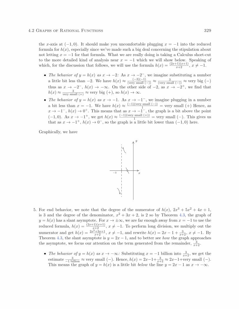
the x-axis at (−1, 0). It should make you uncomfortable plugging x = −1 into the reducedformula for h(x), especially since we’ve made such a big deal concerning the stipulation aboutnot letting x = −1 for that formula. What we are really doing is taking a Calculus short-cutto the more detailed kind of analysis near x = −1 which we will show below. Speaking ofwhich, for the discussion that follows, we will use the formula h(x) = (2x+1)(x+1)
x+2 , x �= −1.
� The behavior of y = h(x) as x → −2: As x → −2−, we imagine substituting a number
a little bit less than −2. We have h(x) ≈ (−3)(−1)(very small (−)) ≈ 3
(very small (−)) ≈ very big (−)thus as x → −2−, h(x) → −∞. On the other side of −2, as x → −2+, we find thath(x) ≈ 3
very small (+) ≈ very big (+), so h(x)→∞.
� The behavior of y = h(x) as x → −1. As x → −1−, we imagine plugging in a number
a bit less than x = −1. We have h(x) ≈ (−1)(very small (−))1 = very small (+) Hence, as
x→ −1−, h(x)→ 0+. This means that as x→ −1−, the graph is a bit above the point
(−1, 0). As x → −1+, we get h(x) ≈ (−1)(very small (+))1 = very small (−). This gives us
that as x→ −1+, h(x)→ 0−, so the graph is a little bit lower than (−1, 0) here.
Graphically, we have
x
y
−3
5. For end behavior, we note that the degree of the numerator of h(x), 2x3 + 5x2 + 4x + 1,is 3 and the degree of the denominator, x2 + 3x + 2, is 2 so by Theorem 4.3, the graph ofy = h(x) has a slant asymptote. For x→ ±∞, we are far enough away from x = −1 to use the
reduced formula, h(x) = (2x+1)(x+1)x+2 , x �= −1. To perform long division, we multiply out the
numerator and get h(x) = 2x2+3x+1x+2 , x �= −1, and rewrite h(x) = 2x− 1 + 3
x+2 , x �= −1. ByTheorem 4.3, the slant asymptote is y = 2x− 1, and to better see how the graph approachesthe asymptote, we focus our attention on the term generated from the remainder, 3
x+2 .
� The behavior of y = h(x) as x→ −∞: Substituting x = −1 billion into 3x+2 , we get the
estimate 3−1 billion ≈ very small (−). Hence, h(x) = 2x−1+ 3
x+2 ≈ 2x−1+very small (−).This means the graph of y = h(x) is a little bit below the line y = 2x− 1 as x→ −∞.

330 Rational Functions
� The behavior of y = h(x) as x→∞: If x→∞, then 3x+2 ≈ very small (+). This means
h(x) ≈ 2x − 1 + very small (+), or that the graph of y = h(x) is a little bit above theline y = 2x− 1 as x→∞.
Graphically we have
x
y
−4
−3
−2
−1
1
2
3
4
6. To make our sign diagram, we place an ‘�’ above x = −2 and x = −1 and a ‘0’ above x = −12 .
On our four test intervals, we find h(x) is (+) on (−2,−1) and (−12 ,∞
)and h(x) is (−) on
(−∞,−2) and (−1,−12
). Putting all of our work together yields the graph below.
−2 −1 −12
(−) � (+) � (−) 0 (+) x
y
−4 −3 −1 1 2 3 4
−14
−13
−12
−11
−10
−9
−8
−7
−6
−5
−4
−3
−2
−1
1
2
3
4
5
6
7
8
9
We could ask whether the graph of y = h(x) crosses its slant asymptote. From the formulah(x) = 2x− 1 + 3
x+2 , x �= −1, we see that if h(x) = 2x− 1, we would have 3x+2 = 0. Since this will
never happen, we conclude the graph never crosses its slant asymptote.14
14But rest assured, some graphs do!

4.2 Graphs of Rational Functions 331
We end this section with an example that shows it’s not all pathological weirdness when it comesto rational functions and technology still has a role to play in studying their graphs at this level.
Example 4.2.4. Sketch the graph of r(x) =x4 + 1
x2 + 1.
Solution.
1. The denominator x2 + 1 is never zero so the domain is (−∞,∞).
2. With no real zeros in the denominator, x2 + 1 is an irreducible quadratic. Our only hope ofreducing r(x) is if x2 + 1 is a factor of x4 + 1. Performing long division gives us
x4 + 1
x2 + 1= x2 − 1 +
2
x2 + 1
The remainder is not zero so r(x) is already reduced.
3. To find the x-intercept, we’d set r(x) = 0. Since there are no real solutions to x4+1x2+1
= 0, wehave no x-intercepts. Since r(0) = 1, we get (0, 1) as the y-intercept.
4. This step doesn’t apply to r, since its domain is all real numbers.
5. For end behavior, we note that since the degree of the numerator is exactly two more thanthe degree of the denominator, neither Theorems 4.2 nor 4.3 apply.15 We know from ourattempt to reduce r(x) that we can rewrite r(x) = x2 − 1 + 2
x2+1, so we focus our attention
on the term corresponding to the remainder, 2x2+1
It should be clear that as x → ±∞,2
x2+1≈ very small (+), which means r(x) ≈ x2 − 1 + very small (+). So the graph y = r(x)
is a little bit above the graph of the parabola y = x2 − 1 as x→ ±∞. Graphically,
1
2
3
4
5
x
y
6. There isn’t much work to do for a sign diagram for r(x), since its domain is all real numbersand it has no zeros. Our sole test interval is (−∞,∞), and since we know r(0) = 1, weconclude r(x) is (+) for all real numbers. At this point, we don’t have much to go on for
15This won’t stop us from giving it the old community college try, however!

332 Rational Functions
a graph.16 Below is a comparison of what we have determined analytically versus what thecalculator shows us. We have no way to detect the relative extrema analytically17 apart frombrute force plotting of points, which is done more efficiently by the calculator.
x
y
−3 −1 1 2 3
1
2
3
4
5
6
As usual, the authors offer no apologies for what may be construed as ‘pedantry’ in this section.We feel that the detail presented in this section is necessary to obtain a firm grasp of the conceptspresented here and it also serves as an introduction to the methods employed in Calculus. As wehave said many times in the past, your instructor will decide how much, if any, of the kinds ofdetails presented here are ‘mission critical’ to your understanding of Precalculus. Without furtherdelay, we present you with this section’s Exercises.
16So even Jeff at this point may check for symmetry! We leave it to the reader to show r(−x) = r(x) so r is even,and, hence, its graph is symmetric about the y-axis.
17Without appealing to Calculus, of course.

4.2 Graphs of Rational Functions 333
4.2.1 Exercises
In Exercises 1 - 16, use the six-step procedure to graph the rational function. Be sure to draw anyasymptotes as dashed lines.
1. f(x) =4
x+ 22. f(x) =
5x
6− 2x
3. f(x) =1
x24. f(x) =
1
x2 + x− 12
5. f(x) =2x− 1
−2x2 − 5x+ 36. f(x) =
x
x2 + x− 12
7. f(x) =4x
x2 + 48. f(x) =
4x
x2 − 4
9. f(x) =x2 − x− 12
x2 + x− 610. f(x) =
3x2 − 5x− 2
x2 − 9
11. f(x) =x2 − x− 6
x+ 112. f(x) =
x2 − x
3− x
13. f(x) =x3 + 2x2 + x
x2 − x− 214. f(x) =
−x3 + 4x
x2 − 9
15. f(x) =x3 − 2x2 + 3x
2x2 + 216.18 f(x) =
x2 − 2x+ 1
x3 + x2 − 2x
In Exercises 17 - 20, graph the rational function by applying transformations to the graph of y =1
x.
17. f(x) =1
x− 218. g(x) = 1− 3
x
19. h(x) =−2x+ 1
x(Hint: Divide) 20. j(x) =
3x− 7
x− 2(Hint: Divide)
21. Discuss with your classmates how you would graph f(x) =ax+ b
cx+ d. What restrictions must
be placed on a, b, c and d so that the graph is indeed a transformation of y =1
x?
22. In Example 3.1.1 in Section 3.1 we showed that p(x) = 4x+x3
x is not a polynomial even thoughits formula reduced to 4 + x2 for x �= 0. However, it is a rational function similar to thosestudied in the section. With the help of your classmates, graph p(x).
18Once you’ve done the six-step procedure, use your calculator to graph this function on the viewing window[0, 12]× [0, 0.25]. What do you see?

334 Rational Functions
23. Let g(x) =x4 − 8x3 + 24x2 − 72x+ 135
x3 − 9x2 + 15x− 7. With the help of your classmates, find the x- and
y- intercepts of the graph of g. Find the intervals on which the function is increasing, theintervals on which it is decreasing and the local extrema. Find all of the asymptotes of thegraph of g and any holes in the graph, if they exist. Be sure to show all of your work includingany polynomial or synthetic division. Sketch the graph of g, using more than one picture ifnecessary to show all of the important features of the graph.
Example 4.2.4 showed us that the six-step procedure cannot tell us everything of importance aboutthe graph of a rational function. Without Calculus, we need to use our graphing calculators toreveal the hidden mysteries of rational function behavior. Working with your classmates, use agraphing calculator to examine the graphs of the rational functions given in Exercises 24 - 27.Compare and contrast their features. Which features can the six-step process reveal and whichfeatures cannot be detected by it?
24. f(x) =1
x2 + 125. f(x) =
x
x2 + 126. f(x) =
x2
x2 + 127. f(x) =
x3
x2 + 1

4.2 Graphs of Rational Functions 335
4.2.2 Answers
1. f(x) =4
x+ 2Domain: (−∞,−2) ∪ (−2,∞)No x-interceptsy-intercept: (0, 2)Vertical asymptote: x = −2As x→ −2−, f(x)→ −∞As x→ −2+, f(x)→∞Horizontal asymptote: y = 0As x→ −∞, f(x)→ 0−
As x→∞, f(x)→ 0+
x
y
−7−6−5−4−3−2−1 1 2 3 4 5
−5
−4
−3
−2
−1
1
2
3
4
5
2. f(x) =5x
6− 2xDomain: (−∞, 3) ∪ (3,∞)x-intercept: (0, 0)y-intercept: (0, 0)Vertical asymptote: x = 3As x→ 3−, f(x)→∞As x→ 3+, f(x)→ −∞Horizontal asymptote: y = −5
2
As x→ −∞, f(x)→ −52
+
As x→∞, f(x)→ −52
−
x
y
−3−2−1 1 2 3 4 5 6 7 8 9
−7
−6
−5
−4
−3
−2
−1
1
2
3
3. f(x) =1
x2Domain: (−∞, 0) ∪ (0,∞)No x-interceptsNo y-interceptsVertical asymptote: x = 0As x→ 0−, f(x)→∞As x→ 0+, f(x)→∞Horizontal asymptote: y = 0As x→ −∞, f(x)→ 0+
As x→∞, f(x)→ 0+x
y
−4 −3 −2 −1 1 2 3 4
1
2
3
4
5
336 Rational Functions
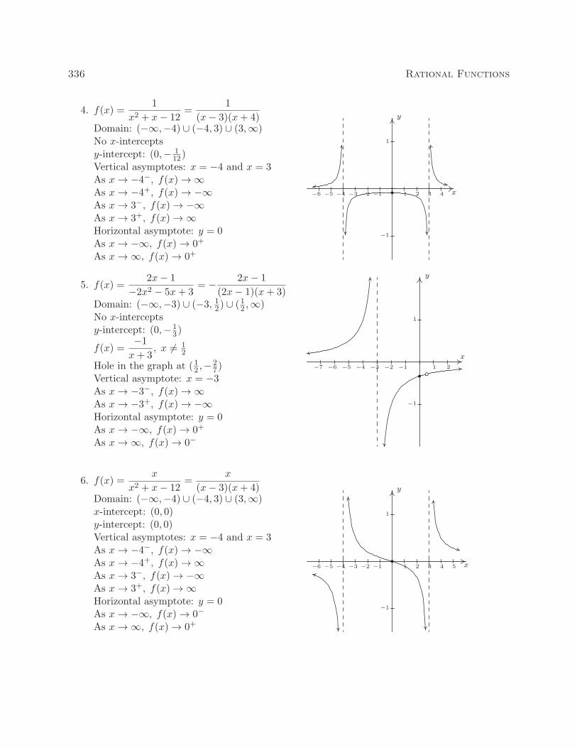
4. f(x) =1
x2 + x− 12=
1
(x− 3)(x+ 4)Domain: (−∞,−4) ∪ (−4, 3) ∪ (3,∞)No x-interceptsy-intercept: (0,− 1
12)Vertical asymptotes: x = −4 and x = 3As x→ −4−, f(x)→∞As x→ −4+, f(x)→ −∞As x→ 3−, f(x)→ −∞As x→ 3+, f(x)→∞Horizontal asymptote: y = 0As x→ −∞, f(x)→ 0+
As x→∞, f(x)→ 0+
x
y
−6 −5 −4 −3 −2 −1 1 2 3 4
−1
1
5. f(x) =2x− 1
−2x2 − 5x+ 3= − 2x− 1
(2x− 1)(x+ 3)Domain: (−∞,−3) ∪ (−3, 12) ∪ (12 ,∞)No x-interceptsy-intercept: (0,−1
3)
f(x) =−1
x+ 3, x �= 1
2
Hole in the graph at (12 ,−27)
Vertical asymptote: x = −3As x→ −3−, f(x)→∞As x→ −3+, f(x)→ −∞Horizontal asymptote: y = 0As x→ −∞, f(x)→ 0+
As x→∞, f(x)→ 0−
x
y
−7 −6 −5 −4 −3 −2 −1 1 2
−1
1
6. f(x) =x
x2 + x− 12=
x
(x− 3)(x+ 4)Domain: (−∞,−4) ∪ (−4, 3) ∪ (3,∞)x-intercept: (0, 0)y-intercept: (0, 0)Vertical asymptotes: x = −4 and x = 3As x→ −4−, f(x)→ −∞As x→ −4+, f(x)→∞As x→ 3−, f(x)→ −∞As x→ 3+, f(x)→∞Horizontal asymptote: y = 0As x→ −∞, f(x)→ 0−
As x→∞, f(x)→ 0+
x
y
−6 −5 −4 −3 −2 −1 1 2 3 4 5
−1
1

4.2 Graphs of Rational Functions 337
7. f(x) =4x
x2 + 4Domain: (−∞,∞)x-intercept: (0, 0)y-intercept: (0, 0)No vertical asymptotesNo holes in the graphHorizontal asymptote: y = 0As x→ −∞, f(x)→ 0−
As x→∞, f(x)→ 0+
x
y
−7−6−5−4−3−2−1 1 2 3 4 5 6 7
−1
1
8. f(x) =4x
x2 − 4=
4x
(x+ 2)(x− 2)Domain: (−∞,−2) ∪ (−2, 2) ∪ (2,∞)x-intercept: (0, 0)y-intercept: (0, 0)Vertical asymptotes: x = −2, x = 2As x→ −2−, f(x)→ −∞As x→ −2+, f(x)→∞As x→ 2−, f(x)→ −∞As x→ 2+, f(x)→∞No holes in the graphHorizontal asymptote: y = 0As x→ −∞, f(x)→ 0−
As x→∞, f(x)→ 0+
x
y
−5 −4 −3 −2 −1 1 2 3 4 5
−5
−4
−3
−2
−1
1
2
3
4
5
9. f(x) =x2 − x− 12
x2 + x− 6=
x− 4
x− 2x �= −3
Domain: (−∞,−3) ∪ (−3, 2) ∪ (2,∞)x-intercept: (4, 0)y-intercept: (0, 2)Vertical asymptote: x = 2As x→ 2−, f(x)→∞As x→ 2+, f(x)→ −∞Hole at
(−3, 75)Horizontal asymptote: y = 1As x→ −∞, f(x)→ 1+
As x→∞, f(x)→ 1−
x
y
−5 −4 −3 −2 −1 1 2 3 4 5
−5
−4
−3
−2
−1
1
2
3
4
5

338 Rational Functions
10. f(x) =3x2 − 5x− 2
x2 − 9=
(3x+ 1)(x− 2)
(x+ 3)(x− 3)Domain: (−∞,−3) ∪ (−3, 3) ∪ (3,∞)x-intercepts:
(−13 , 0
), (2, 0)
y-intercept:(0, 29
)Vertical asymptotes: x = −3, x = 3As x→ −3−, f(x)→∞As x→ −3+, f(x)→ −∞As x→ 3−, f(x)→ −∞As x→ 3+, f(x)→∞No holes in the graphHorizontal asymptote: y = 3As x→ −∞, f(x)→ 3+
As x→∞, f(x)→ 3−
x
y
−9−8−7−7−6−5−4−3−2−1 1 2 3 4 5 6 7 8 9
−9
−8
−7
−6
−5
−4
−3
−2
−1
1
2
3
4
5
6
7
8
9
11. f(x) =x2 − x− 6
x+ 1=
(x− 3)(x+ 2)
x+ 1Domain: (−∞,−1) ∪ (−1,∞)x-intercepts: (−2, 0), (3, 0)y-intercept: (0,−6)Vertical asymptote: x = −1As x→ −1−, f(x)→∞As x→ −1+, f(x)→ −∞Slant asymptote: y = x− 2As x→ −∞, the graph is above y = x− 2As x→∞, the graph is below y = x− 2
x
y
−4−3−2−1 1 2 3 4
−6
−4
−2
2
4
6
8
9
1
3
5
7
12. f(x) =x2 − x
3− x=
x(x− 1)
3− xDomain: (−∞, 3) ∪ (3,∞)x-intercepts: (0, 0), (1, 0)y-intercept: (0, 0)Vertical asymptote: x = 3As x→ 3−, f(x)→∞As x→ 3+, f(x)→ −∞Slant asymptote: y = −x− 2As x→ −∞, the graph is above y = −x− 2As x→∞, the graph is below y = −x− 2
x
y
−8−7−6−5−4−3−2−1 1 2 3 4 5 6 7 8 9 10
−12
−14
−16
−18
−10
−8
−6
−4
−2
2
4
6
8

4.2 Graphs of Rational Functions 339
13. f(x) =x3 + 2x2 + x
x2 − x− 2=
x(x+ 1)
x− 2x �= −1
Domain: (−∞,−1) ∪ (−1, 2) ∪ (2,∞)x-intercept: (0, 0)y-intercept: (0, 0)Vertical asymptote: x = 2As x→ 2−, f(x)→ −∞As x→ 2+, f(x)→∞Hole at (−1, 0)Slant asymptote: y = x+ 3As x→ −∞, the graph is below y = x+ 3As x→∞, the graph is above y = x+ 3
x
y
−9−8−7−6−5−4−3−2−1 1 2 3 4 5 6 7 8 9
−10
−8
−6
−4
−2
2
4
6
8
10
12
14
16
18
14. f(x) =−x3 + 4x
x2 − 9Domain: (−∞,−3) ∪ (−3, 3) ∪ (3,∞)x-intercepts: (−2, 0), (0, 0), (2, 0)y-intercept: (0, 0)Vertical asymptotes: x = −3, x = 3As x→ −3−, f(x)→∞As x→ −3+, f(x)→ −∞As x→ 3−, f(x)→∞As x→ 3+, f(x)→ −∞Slant asymptote: y = −xAs x→ −∞, the graph is above y = −xAs x→∞, the graph is below y = −x
x
y
−6−5−4−3−2−1 1 2 3 4 5 6
−7
−6
−5
−4
−3
−2
−1
1
2
3
4
5
6
7
15. f(x) =x3 − 2x2 + 3x
2x2 + 2Domain: (−∞,∞)x-intercept: (0, 0)y-intercept: (0, 0)Slant asymptote: y = 1
2x− 1As x→ −∞, the graph is below y = 1
2x− 1As x→∞, the graph is above y = 1
2x− 1
x
y
−4 −3 −2 −1 1 2 3 4
−2
−1
1
2

340 Rational Functions
16. f(x) =x2 − 2x+ 1
x3 + x2 − 2xDomain: (−∞,−2) ∪ (−2, 0) ∪ (0, 1) ∪ (1,∞)
f(x) =x− 1
x(x+ 2), x �= 1
No x-interceptsNo y-interceptsVertical asymptotes: x = −2 and x = 0As x→ −2−, f(x)→ −∞As x→ −2+, f(x)→∞As x→ 0−, f(x)→∞As x→ 0+, f(x)→ −∞Hole in the graph at (1, 0)Horizontal asymptote: y = 0As x→ −∞, f(x)→ 0−
As x→∞, f(x)→ 0+
x
y
−5 −4 −3 −2 −1 1 2 3 4 5
−5
−4
−3
−2
−1
1
2
3
4
5
17. f(x) =1
x− 2
Shift the graph of y =1
xto the right 2 units.
x
y
−1 1 2 3 4 5
−3
−2
−1
1
2
3
18. g(x) = 1− 3
x
Vertically stretch the graph of y =1
xby a factor of 3.
Reflect the graph of y =3
xabout the x-axis.
Shift the graph of y = −3
xup 1 unit.
x
y
−6−5−4−3−2−1 1 2 3 4 5 6
−5
−4
−3
−2
−1
1
2
3
4
5
6
7

4.2 Graphs of Rational Functions 341
19. h(x) =−2x+ 1
x= −2 + 1
x
Shift the graph of y =1
xdown 2 units. x
y
−3 −2 −1 1 2 3
−5
−4
−3
−2
−1
1
20. j(x) =3x− 7
x− 2= 3− 1
x− 2
Shift the graph of y =1
xto the right 2 units.
Reflect the graph of y =1
x− 2about the x-axis.
Shift the graph of y = − 1
x− 2up 3 units.
x
y
−3 −2 −1 1 2 3 4 5
−1
1
2
3
4
5
6
7

342 Rational Functions
4.3 Rational Inequalities and Applications
In this section, we solve equations and inequalities involving rational functions and explore associ-ated application problems. Our first example showcases the critical difference in procedure betweensolving a rational equation and a rational inequality.
Example 4.3.1.
1. Solvex3 − 2x+ 1
x− 1=
1
2x− 1. 2. Solve
x3 − 2x+ 1
x− 1≥ 1
2x− 1.
3. Use your calculator to graphically check your answers to 1 and 2.
Solution.
1. To solve the equation, we clear denominators
x3 − 2x+ 1
x− 1=
1
2x− 1
(x3 − 2x+ 1
x− 1
)· 2(x− 1) =
(1
2x− 1
)· 2(x− 1)
2x3 − 4x+ 2 = x2 − 3x+ 2 expand2x3 − x2 − x = 0
x(2x+ 1)(x− 1) = 0 factorx = −1
2 , 0, 1
Since we cleared denominators, we need to check for extraneous solutions. Sure enough, wesee that x = 1 does not satisfy the original equation and must be discarded. Our solutionsare x = −1
2 and x = 0.
2. To solve the inequality, it may be tempting to begin as we did with the equation − namelyby multiplying both sides by the quantity (x − 1). The problem is that, depending on x,(x − 1) may be positive (which doesn’t affect the inequality) or (x − 1) could be negative(which would reverse the inequality). Instead of working by cases, we collect all of the termson one side of the inequality with 0 on the other and make a sign diagram using the techniquegiven on page 321 in Section 4.2.
x3 − 2x+ 1
x− 1≥ 1
2x− 1
x3 − 2x+ 1
x− 1− 1
2x+ 1 ≥ 0
2(x3 − 2x+ 1
)− x(x− 1) + 1(2(x− 1))
2(x− 1)≥ 0 get a common denominator
2x3 − x2 − x
2x− 2≥ 0 expand

4.3 Rational Inequalities and Applications 343
Viewing the left hand side as a rational function r(x) we make a sign diagram. The onlyvalue excluded from the domain of r is x = 1 which is the solution to 2x− 2 = 0. The zerosof r are the solutions to 2x3 − x2 − x = 0, which we have already found to be x = 0, x = −1
2and x = 1, the latter was discounted as a zero because it is not in the domain. Choosing testvalues in each test interval, we construct the sign diagram below.
−12
0 1
(+) 0 (−) 0 (+) � (+)
We are interested in where r(x) ≥ 0. We find r(x) > 0, or (+), on the intervals(−∞,−1
2
),
(0, 1) and (1,∞). We add to these intervals the zeros of r, −12 and 0, to get our final solution:(−∞,−1
2
] ∪ [0, 1) ∪ (1,∞).
3. Geometrically, if we set f(x) = x3−2x+1x−1 and g(x) = 1
2x− 1, the solutions to f(x) = g(x) arethe x-coordinates of the points where the graphs of y = f(x) and y = g(x) intersect. Thesolution to f(x) ≥ g(x) represents not only where the graphs meet, but the intervals overwhich the graph of y = f(x) is above (>) the graph of g(x). We obtain the graphs below.
The ‘Intersect’ command confirms that the graphs cross when x = −12 and x = 0. It is clear
from the calculator that the graph of y = f(x) is above the graph of y = g(x) on(−∞,−1
2
)as well as on (0,∞). According to the calculator, our solution is then
(−∞,−12
] ∪ [0,∞)which almost matches the answer we found analytically. We have to remember that f is notdefined at x = 1, and, even though it isn’t shown on the calculator, there is a hole1 in thegraph of y = f(x) when x = 1 which is why x = 1 is not part of our final answer.
Next, we explore how rational equations can be used to solve some classic problems involving rates.
Example 4.3.2. Carl decides to explore the Meander River, the location of several recent Sasquatchsightings. From camp, he canoes downstream five miles to check out a purported Sasquatch nest.Finding nothing, he immediately turns around, retraces his route (this time traveling upstream),
1There is no asymptote at x = 1 since the graph is well behaved near x = 1. According to Theorem 4.1, theremust be a hole there.

344 Rational Functions
and returns to camp 3 hours after he left. If Carl canoes at a rate of 6 miles per hour in still water,how fast was the Meander River flowing on that day?
Solution. We are given information about distances, rates (speeds) and times. The basic principlerelating these quantities is:
distance = rate · time
The first observation to make, however, is that the distance, rate and time given to us aren’t‘compatible’: the distance given is the distance for only part of the trip, the rate given is the speedCarl can canoe in still water, not in a flowing river, and the time given is the duration of the entiretrip. Ultimately, we are after the speed of the river, so let’s call that R measured in miles per hourto be consistent with the other rate given to us. To get started, let’s divide the trip into its twoparts: the initial trip downstream and the return trip upstream. For the downstream trip, all weknow is that the distance traveled is 5 miles.
distance downstream = rate traveling downstream · time traveling downstream5miles = rate traveling downstream · time traveling downstream
Since the return trip upstream followed the same route as the trip downstream, we know that thedistance traveled upstream is also 5 miles.
distance upstream = rate traveling upstream · time traveling upstream5miles = rate traveling upstream · time traveling upstream
We are told Carl can canoe at a rate of 6 miles per hour in still water. How does this figureinto the rates traveling upstream and downstream? The speed the canoe travels in the river is acombination of the speed at which Carl can propel the canoe in still water, 6 miles per hour, andthe speed of the river, which we’re calling R. When traveling downstream, the river is helping Carlalong, so we add these two speeds:
rate traveling downstream = rate Carl propels the canoe + speed of the river
= 6mileshour +Rmiles
hour
So our downstream speed is (6 + R)mileshour . Substituting this into our ‘distance-rate-time’ equation
for the downstream part of the trip, we get:
5miles = rate traveling downstream · time traveling downstream
5miles = (6 +R)mileshour · time traveling downstream
When traveling upstream, Carl works against the current. Since the canoe manages to travelupstream, the speed Carl can canoe in still water is greater than the river’s speed, so we subtractthe river’s speed from Carl’s canoing speed to get:
rate traveling upstream = rate Carl propels the canoe− river speed
= 6mileshour −Rmiles
hour
Proceeding as before, we get

4.3 Rational Inequalities and Applications 345
5miles = rate traveling upstream · time traveling upstream
5miles = (6−R)mileshour · time traveling upstream
The last piece of information given to us is that the total trip lasted 3 hours. If we let tdown denotethe time of the downstream trip and tup the time of the upstream trip, we have: tdown+tup = 3hours.Substituting tdown and tup into the ‘distance-rate-time’ equations, we get (suppressing the units)three equations in three unknowns:2
⎧⎨⎩
E1 (6 +R) tdown = 5E2 (6−R) tup = 5E3 tdown + tup = 3
Since we are ultimately after R, we need to use these three equations to get at least one equationinvolving only R. To that end, we solve E1 for tdown by dividing both sides3 by the quantity (6+R)to get tdown = 5
6+R . Similarly, we solve E2 for tup and get tup = 56−R . Substituting these into E3,
we get:4
5
6 +R+
5
6−R= 3.
Clearing denominators, we get 5(6− R) + 5(6 + R) = 3(6 + R)(6− R) which reduces to R2 = 16.We find R = ±4, and since R represents the speed of the river, we choose R = 4. On the day inquestion, the Meander River is flowing at a rate of 4 miles per hour.
One of the important lessons to learn from Example 4.3.2 is that speeds, and more generally, rates,are additive. As we see in our next example, the concept of rate and its associated principles canbe applied to a wide variety of problems - not just ‘distance-rate-time’ scenarios.
Example 4.3.3. Working alone, Taylor can weed the garden in 4 hours. If Carl helps, they canweed the garden in 3 hours. How long would it take for Carl to weed the garden on his own?
Solution. The key relationship between work and time which we use in this problem is:
amount of work done = rate of work · time spent working
We are told that, working alone, Taylor can weed the garden in 4 hours. In Taylor’s case then:
amount of work Taylor does = rate of Taylor working · time Taylor spent working1 garden = (rate of Taylor working) · (4 hours)
So we have that the rate Taylor works is 1 garden4 hours = 1
4gardenhour . We are also told that when working
together, Taylor and Carl can weed the garden in just 3 hours. We have:
2This is called a system of equations. No doubt, you’ve had experience with these things before, and we will studysystems in greater detail in Chapter 8.
3While we usually discourage dividing both sides of an equation by a variable expression, we know (6 + R) �= 0since otherwise we couldn’t possibly multiply it by tdown and get 5.
4The reader is encouraged to verify that the units in this equation are the same on both sides. To get you started,the units on the ‘3’ is ‘hours.’

346 Rational Functions
amount of work done together = rate of working together · time spent working together1 garden = (rate of working together) · (3 hours)
From this, we find that the rate of Taylor and Carl working together is 1 garden3 hours = 1
3gardenhour . We are
asked to find out how long it would take for Carl to weed the garden on his own. Let us call thisunknown t, measured in hours to be consistent with the other times given to us in the problem.Then:
amount of work Carl does = rate of Carl working · time Carl spent working1 garden = (rate of Carl working) · (t hours)
In order to find t, we need to find the rate of Carl working, so let’s call this quantity R, with unitsgardenhour . Using the fact that rates are additive, we have:
rate working together = rate of Taylor working + rate of Carl working
13gardenhour = 1
4gardenhour +R garden
hour
so that R = 112
gardenhour . Substituting this into our ‘work-rate-time’ equation for Carl, we get:
1 garden = (rate of Carl working) · (t hours)1 garden =
(112
gardenhour
)· (t hours)
Solving 1 = 112 t, we get t = 12, so it takes Carl 12 hours to weed the garden on his own.5
As is common with ‘word problems’ like Examples 4.3.2 and 4.3.3, there is no short-cut to theanswer. We encourage the reader to carefully think through and apply the basic principles of rateto each (potentially different!) situation. It is time well spent. We also encourage the tracking ofunits, especially in the early stages of the problem. Not only does this promote uniformity in theunits, it also serves as a quick means to check if an equation makes sense.6
Our next example deals with the average cost function, first introduced on page 82, as applied toPortaBoy Game systems from Example 2.1.5 in Section 2.1.
Example 4.3.4. Given a cost function C(x), which returns the total cost of producing x items,
recall that the average cost function, C(x) = C(x)x computes the cost per item when x items are
produced. Suppose the cost C, in dollars, to produce x PortaBoy game systems for a local retaileris C(x) = 80x+ 150, x ≥ 0.
1. Find an expression for the average cost function C(x).
2. Solve C(x) < 100 and interpret.
5Carl would much rather spend his time writing open-source Mathematics texts than gardening anyway.6In other words, make sure you don’t try to add apples to oranges!

4.3 Rational Inequalities and Applications 347
3. Determine the behavior of C(x) as x→∞ and interpret.
Solution.
1. From C(x) = C(x)x , we obtain C(x) = 80x+150
x . The domain of C is x ≥ 0, but since x = 0causes problems for C(x), we get our domain to be x > 0, or (0,∞).
2. Solving C(x) < 100 means we solve 80x+150x < 100. We proceed as in the previous example.
80x+ 150
x< 100
80x+ 150
x− 100 < 0
80x+ 150− 100x
x< 0 common denominator
150− 20x
x< 0
If we take the left hand side to be a rational function r(x), we need to keep in mind that theapplied domain of the problem is x > 0. This means we consider only the positive half of thenumber line for our sign diagram. On (0,∞), r is defined everywhere so we need only lookfor zeros of r. Setting r(x) = 0 gives 150− 20x = 0, so that x = 15
2 = 7.5. The test intervalson our domain are (0, 7.5) and (7.5,∞). We find r(x) < 0 on (7.5,∞).
0
�
7.5
(+) 0 (−)
In the context of the problem, x represents the number of PortaBoy games systems producedand C(x) is the average cost to produce each system. Solving C(x) < 100 means we are tryingto find how many systems we need to produce so that the average cost is less than $100 persystem. Our solution, (7.5,∞) tells us that we need to produce more than 7.5 systems toachieve this. Since it doesn’t make sense to produce half a system, our final answer is [8,∞).
3. When we apply Theorem 4.2 to C(x) we find that y = 80 is a horizontal asymptote tothe graph of y = C(x). To more precisely determine the behavior of C(x) as x → ∞, wefirst use long division7 and rewrite C(x) = 80 + 150
x . As x → ∞, 150x → 0+, which means
C(x) ≈ 80 + very small (+). Thus the average cost per system is getting closer to $80 persystem. If we set C(x) = 80, we get 150
x = 0, which is impossible, so we conclude thatC(x) > 80 for all x > 0. This means that the average cost per system is always greater than$80 per system, but the average cost is approaching this amount as more and more systemsare produced. Looking back at Example 2.1.5, we realize $80 is the variable cost per system −
7In this case, long division amounts to term-by-term division.
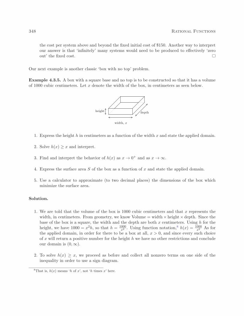
348 Rational Functions
the cost per system above and beyond the fixed initial cost of $150. Another way to interpretour answer is that ‘infinitely’ many systems would need to be produced to effectively ‘zeroout’ the fixed cost.
Our next example is another classic ‘box with no top’ problem.
Example 4.3.5. A box with a square base and no top is to be constructed so that it has a volumeof 1000 cubic centimeters. Let x denote the width of the box, in centimeters as seen below.
width, x
height depth
1. Express the height h in centimeters as a function of the width x and state the applied domain.
2. Solve h(x) ≥ x and interpret.
3. Find and interpret the behavior of h(x) as x→ 0+ and as x→∞.
4. Express the surface area S of the box as a function of x and state the applied domain.
5. Use a calculator to approximate (to two decimal places) the dimensions of the box whichminimize the surface area.
Solution.
1. We are told that the volume of the box is 1000 cubic centimeters and that x represents thewidth, in centimeters. From geometry, we know Volume = width× height× depth. Since thebase of the box is a square, the width and the depth are both x centimeters. Using h for theheight, we have 1000 = x2h, so that h = 1000
x2 . Using function notation,8 h(x) = 1000x2 As for
the applied domain, in order for there to be a box at all, x > 0, and since every such choiceof x will return a positive number for the height h we have no other restrictions and concludeour domain is (0,∞).
2. To solve h(x) ≥ x, we proceed as before and collect all nonzero terms on one side of theinequality in order to use a sign diagram.
8That is, h(x) means ‘h of x’, not ‘h times x’ here.

4.3 Rational Inequalities and Applications 349
h(x) ≥ x
1000
x2≥ x
1000
x2− x ≥ 0
1000− x3
x2≥ 0 common denominator
We consider the left hand side of the inequality as our rational function r(x). We see r isundefined at x = 0, but, as in the previous example, the applied domain of the problem isx > 0, so we are considering only the behavior of r on (0,∞). The sole zero of r comes when1000−x3 = 0, which is x = 10. Choosing test values in the intervals (0, 10) and (10,∞) givesthe following diagram.
0
� (+)
10
0 (−)
We see r(x) > 0 on (0, 10), and since r(x) = 0 at x = 10, our solution is (0, 10]. In the contextof the problem, h represents the height of the box while x represents the width (and depth)of the box. Solving h(x) ≥ x is tantamount to finding the values of x which result in a boxwhere the height is at least as big as the width (and, in this case, depth.) Our answer tellsus the width of the box can be at most 10 centimeters for this to happen.
3. As x → 0+, h(x) = 1000x2 → ∞. This means that the smaller the width x (and, in this
case, depth), the larger the height h has to be in order to maintain a volume of 1000 cubiccentimeters. As x→∞, we find h(x)→ 0+, which means that in order to maintain a volumeof 1000 cubic centimeters, the width and depth must get bigger as the height becomes smaller.
4. Since the box has no top, the surface area can be found by adding the area of each of thesides to the area of the base. The base is a square of dimensions x by x, and each side hasdimensions x by h. We get the surface area, S = x2 + 4xh. To get S as a function of x, wesubstitute h = 1000
x2 to obtain S = x2+4x(1000x2
). Hence, as a function of x, S(x) = x2+ 4000
x .The domain of S is the same as h, namely (0,∞), for the same reasons as above.
5. A first attempt at the graph of y = S(x) on the calculator may lead to frustration. Chancesare good that the first window chosen to view the graph will suggest y = S(x) has the x-axisas a horizontal asymptote. From the formula S(x) = x2+ 4000
x , however, we get S(x) ≈ x2 asx→∞, so S(x)→∞. Readjusting the window, we find S does possess a relative minimumat x ≈ 12.60. As far as we can tell,9 this is the only relative extremum, so it is the absoluteminimum as well. This means that the width and depth of the box should each measure
9without Calculus, that is...

350 Rational Functions
approximately 12.60 centimeters. To determine the height, we find h(12.60) ≈ 6.30, so theheight of the box should be approximately 6.30 centimeters.
4.3.1 Variation
In many instances in the sciences, rational functions are encountered as a result of fundamentalnatural laws which are typically a result of assuming certain basic relationships between variables.These basic relationships are summarized in the definition below.
Definition 4.5. Suppose x, y and z are variable quantities. We say
� y varies directly with (or is directly proportional to) x if there is a constant k suchthat y = kx.
� y varies inversely with (or is inversely proportional to) x if there is a constant ksuch that y = k
x .
� z varies jointly with (or is jointly proportional to) x and y if there is a constant ksuch that z = kxy.
The constant k in the above definitions is called the constant of proportionality.
Example 4.3.6. Translate the following into mathematical equations using Definition 4.5.
1. Hooke’s Law: The force F exerted on a spring is directly proportional the extension x of thespring.
2. Boyle’s Law: At a constant temperature, the pressure P of an ideal gas is inversely propor-tional to its volume V .
3. The volume V of a right circular cone varies jointly with the height h of the cone and thesquare of the radius r of the base.
4. Ohm’s Law: The current I through a conductor between two points is directly proportional tothe voltage V between the two points and inversely proportional to the resistance R betweenthe two points.

4.3 Rational Inequalities and Applications 351
5. Newton’s Law of Universal Gravitation: Suppose two objects, one of mass m and one of massM , are positioned so that the distance between their centers of mass is r. The gravitationalforce F exerted on the two objects varies directly with the product of the two masses andinversely with the square of the distance between their centers of mass.
Solution.
1. Applying the definition of direct variation, we get F = kx for some constant k.
2. Since P and V are inversely proportional, we write P = kV .
3. There is a bit of ambiguity here. It’s clear that the volume and the height of the cone arerepresented by the quantities V and h, respectively, but does r represent the radius of the baseor the square of the radius of the base? It is the former. Usually, if an algebraic operation isspecified (like squaring), it is meant to be expressed in the formula. We apply Definition 4.5to get V = khr2.
4. Even though the problem doesn’t use the phrase ‘varies jointly’, it is implied by the fact thatthe current I is related to two different quantities. Since I varies directly with V but inverselywith R, we write I = kV
R .
5. We write the product of the masses mM and the square of the distance as r2. We have thatF varies directly with mM and inversely with r2, so F = kmM
r2.
In many of the formulas in the previous example, more than two varying quantities are related. Inpractice, however, usually all but two quantities are held constant in an experiment and the datacollected is used to relate just two of the variables. Comparing just two varying quantities allowsus to view the relationship between them as functional, as the next example illustrates.
Example 4.3.7. According to this website the actual data relating the volume V of a gas and itspressure P used by Boyle and his assistant in 1662 to verify the gas law that bears his name isgiven below.
V 48 46 44 42 40 38 36 34 32 30 28 26 24
P 29.13 30.56 31.94 33.5 35.31 37 39.31 41.63 44.19 47.06 50.31 54.31 58.81
V 23 22 21 20 19 18 17 16 15 14 13 12
P 61.31 64.06 67.06 70.69 74.13 77.88 82.75 87.88 93.06 100.44 107.81 117.56
1. Use your calculator to generate a scatter diagram for these data using V as the independentvariable and P as the dependent variable. Does it appear from the graph that P is inverselyproportional to V ? Explain.
2. Assuming that P and V do vary inversely, use the data to approximate the constant ofproportionality.

352 Rational Functions
3. Use your calculator to determine a ‘Power Regression’ for this data10 and use it verify yourresults in 1 and 2.
Solution.
1. If P really does vary inversely with V , then P = kV for some constant k. From the data plot,
the points do seem to lie along a curve like y = kx .
2. To determine the constant of proportionality, we note that from P = kV , we get k = PV .
Multiplying each of the volume numbers times each of the pressure numbers,11 we produce anumber which is always approximately 1400. We suspect that P = 1400
V . Graphing y = 1400x
along with the data gives us good reason to believe our hypotheses that P and V are, in fact,inversely related.
The graph of the data The data with y = 1400x
3. After performing a ‘Power Regression’, the calculator fits the data to the curve y = axb wherea ≈ 1400 and b ≈ −1 with a correlation coefficient which is darned near perfect.12 In otherwords, y = 1400x−1 or y = 1400
x , as we guessed.
10We will talk more about this in the coming chapters.11You can use tell the calculator to do this arithmetic on the lists and save yourself some time.12We will revisit this example once we have developed logarithms in Chapter 6 to see how we can actually ‘linearize’
this data and do a linear regression to obtain the same result.

4.3 Rational Inequalities and Applications 353
4.3.2 Exercises
In Exercises 1 - 6, solve the rational equation. Be sure to check for extraneous solutions.
1.x
5x+ 4= 3 2.
3x− 1
x2 + 1= 1
3.1
x+ 3+
1
x− 3=
x2 − 3
x2 − 94.
2x+ 17
x+ 1= x+ 5
5.x2 − 2x+ 1
x3 + x2 − 2x= 1 6.
−x3 + 4x
x2 − 9= 4x
In Exercises 7 - 20, solve the rational inequality. Express your answer using interval notation.
7.1
x+ 2≥ 0 8.
x− 3
x+ 2≤ 0 9.
x
x2 − 1> 0
10.4x
x2 + 4≥ 0 11.
x2 − x− 12
x2 + x− 6> 0 12.
3x2 − 5x− 2
x2 − 9< 0
13.x3 + 2x2 + x
x2 − x− 2≥ 0 14.
x2 + 5x+ 6
x2 − 1> 0 15.
3x− 1
x2 + 1≤ 1
16.2x+ 17
x+ 1> x+ 5 17.
−x3 + 4x
x2 − 9≥ 4x 18.
1
x2 + 1< 0
19.x4 − 4x3 + x2 − 2x− 15
x3 − 4x2≥ x 20.
5x3 − 12x2 + 9x+ 10
x2 − 1≥ 3x− 1
21. Carl and Mike start a 3 mile race at the same time. If Mike ran the race at 6 miles per hourand finishes the race 10 minutes before Carl, how fast does Carl run?
22. One day, Donnie observes that the wind is blowing at 6 miles per hour. A unladen swallownesting near Donnie’s house flies three quarters of a mile down the road (in the direction ofthe wind), turns around, and returns exactly 4 minutes later. What is the airspeed of theunladen swallow? (Here, ‘airspeed’ is the speed that the swallow can fly in still air.)
23. In order to remove water from a flooded basement, two pumps, each rated at 40 gallons perminute, are used. After half an hour, the one pump burns out, and the second pump finishesremoving the water half an hour later. How many gallons of water were removed from thebasement?
24. A faucet can fill a sink in 5 minutes while a drain will empty the same sink in 8 minutes. Ifthe faucet is turned on and the drain is left open, how long will it take to fill the sink?
25. Working together, Daniel and Donnie can clean the llama pen in 45 minutes. On his own,Daniel can clean the pen in an hour. How long does it take Donnie to clean the llama pen onhis own?
354 Rational Functions
26. In Exercise 32, the function C(x) = .03x3 − 4.5x2 + 225x+ 250, for x ≥ 0 was used to modelthe cost (in dollars) to produce x PortaBoy game systems. Using this cost function, find thenumber of PortaBoys which should be produced to minimize the average cost C. Round youranswer to the nearest number of systems.
27. Suppose we are in the same situation as Example 4.3.5. If the volume of the box is to be 500cubic centimeters, use your calculator to find the dimensions of the box which minimize thesurface area. What is the minimum surface area? Round your answers to two decimal places.
28. The box for the new Sasquatch-themed cereal, ‘Crypt-Os’, is to have a volume of 140 cubicinches. For aesthetic reasons, the height of the box needs to be 1.62 times the width of thebase of the box.13 Find the dimensions of the box which will minimize the surface area of thebox. What is the minimum surface area? Round your answers to two decimal places.
29. Sally is Skippy’s neighbor from Exercise 19 in Section 2.3. Sally also wants to plant a vegetablegarden along the side of her home. She doesn’t have any fencing, but wants to keep the sizeof the garden to 100 square feet. What are the dimensions of the garden which will minimizethe amount of fencing she needs to buy? What is the minimum amount of fencing she needsto buy? Round your answers to the nearest foot. (Note: Since one side of the garden willborder the house, Sally doesn’t need fencing along that side.)
30. Another Classic Problem: A can is made in the shape of a right circular cylinder and is tohold one pint. (For dry goods, one pint is equal to 33.6 cubic inches.)14
(a) Find an expression for the volume V of the can in terms of the height h and the baseradius r.
(b) Find an expression for the surface area S of the can in terms of the height h and thebase radius r. (Hint: The top and bottom of the can are circles of radius r and the sideof the can is really just a rectangle that has been bent into a cylinder.)
(c) Using the fact that V = 33.6, write S as a function of r and state its applied domain.
(d) Use your graphing calculator to find the dimensions of the can which has minimal surfacearea.
31. A right cylindrical drum is to hold 7.35 cubic feet of liquid. Find the dimensions (radiusof the base and height) of the drum which would minimize the surface area. What is theminimum surface area? Round your answers to two decimal places.
32. In Exercise 71 in Section 1.4, the population of Sasquatch in Portage County was modeledby the function P (t) = 150t
t+15 , where t = 0 represents the year 1803. When were there fewerthan 100 Sasquatch in Portage County?
131.62 is a crude approximation of the so-called ‘Golden Ratio’ φ = 1+√5
2.
14According to www.dictionary.com, there are different values given for this conversion. We will stick with 33.6in3
for this problem.

4.3 Rational Inequalities and Applications 355
In Exercises 33 - 38, translate the following into mathematical equations.
33. At a constant pressure, the temperature T of an ideal gas is directly proportional to its volumeV . (This is Charles’s Law)
34. The frequency of a wave f is inversely proportional to the wavelength of the wave λ.
35. The density d of a material is directly proportional to the mass of the object m and inverselyproportional to its volume V .
36. The square of the orbital period of a planet P is directly proportional to the cube of thesemi-major axis of its orbit a. (This is Kepler’s Third Law of Planetary Motion )
37. The drag of an object traveling through a fluid D varies jointly with the density of the fluidρ and the square of the velocity of the object ν.
38. Suppose two electric point charges, one with charge q and one with charge Q, are positioned runits apart. The electrostatic force F exerted on the charges varies directly with the productof the two charges and inversely with the square of the distance between the charges. (Thisis Coulomb’s Law)
39. According to this webpage, the frequency f of a vibrating string is given by f =1
2L
√T
μwhere T is the tension, μ is the linear mass15 of the string and L is the length of the vibratingpart of the string. Express this relationship using the language of variation.
40. According to the Centers for Disease Control and Prevention www.cdc.gov, a person’s BodyMass Index B is directly proportional to his weight W in pounds and inversely proportionalto the square of his height h in inches.
(a) Express this relationship as a mathematical equation.
(b) If a person who was 5 feet, 10 inches tall weighed 235 pounds had a Body Mass Indexof 33.7, what is the value of the constant of proportionality?
(c) Rewrite the mathematical equation found in part 40a to include the value of the constantfound in part 40b and then find your Body Mass Index.
41. We know that the circumference of a circle varies directly with its radius with 2π as theconstant of proportionality. (That is, we know C = 2πr.) With the help of your classmates,compile a list of other basic geometric relationships which can be seen as variations.
15Also known as the linear density. It is simply a measure of mass per unit length.
356 Rational Functions
4.3.3 Answers
1. x = −67 2. x = 1, x = 2 3. x = −1
4. x = −6, x = 2 5. No solution 6. x = 0, x = ±2√2
7. (−2,∞) 8. (−2, 3]
9. (−1, 0) ∪ (1,∞) 10. [0,∞)
11. (−∞,−3) ∪ (−3, 2) ∪ (4,∞) 12.(−3,−1
3
) ∪ (2, 3)
13. (−1, 0] ∪ (2,∞) 14. (−∞,−3) ∪ (−2,−1) ∪ (1,∞)
15. (−∞, 1] ∪ [2,∞) 16. (−∞,−6) ∪ (−1, 2)
17. (−∞,−3) ∪ [−2√2, 0] ∪ [
2√2, 3
)18. No solution
19. [−3, 0) ∪ (0, 4) ∪ [5,∞) 20.(−1,−1
2
] ∪ (1,∞)
21. 4.5 miles per hour 22. 24 miles per hour 23. 3600 gallons
24. 403 ≈ 13.33 minutes 25. 3 hours
26. The absolute minimum of y = C(x) occurs at ≈ (75.73, 59.57). Since x represents the numberof game systems, we check C(75) ≈ 59.58 and C(76) ≈ 59.57. Hence, to minimize the averagecost, 76 systems should be produced at an average cost of $59.57 per system.
27. The width (and depth) should be 10.00 centimeters, the height should be 5.00 centimeters.The minimum surface area is 300.00 square centimeters.
28. The width of the base of the box should be ≈ 4.12 inches, the height of the box should be≈ 6.67 inches, and the depth of the base of the box should be ≈ 5.09 inches; minimum surfacearea ≈ 164.91 square inches.
29. The dimensions are ≈ 7 feet by ≈ 14 feet; minimum amount of fencing required ≈ 28 feet.
30. (a) V = πr2h (b) S = 2πr2 + 2πrh
(c) S(r) = 2πr2 + 67.2r , Domain r > 0 (d) r ≈ 1.749 in. and h ≈ 3.498 in.
31. The radius of the drum should be ≈ 1.05 feet and the height of the drum should be ≈ 2.12feet. The minimum surface area of the drum is ≈ 20.93 cubic feet.
32. P (t) < 100 on (−15, 30), and the portion of this which lies in the applied domain is [0, 30).Since t = 0 corresponds to the year 1803, from 1803 through the end of 1832, there werefewer than 100 Sasquatch in Portage County.

4.3 Rational Inequalities and Applications 357
33. T = kV 34. 16 f =k
λ35. d =
km
V
36. P 2 = ka3 37. 17 D = kρν2 38. 18 F =kqQ
r2
39. Rewriting f =1
2L
√T
μas f =
12
√T
L√μ
we see that the frequency f varies directly with the
square root of the tension and varies inversely with the length and the square root of thelinear mass.
40. (a) B =kW
h2(b) 19 k = 702.68 (c) B =
702.68W
h2
16The character λ is the lower case Greek letter ‘lambda.’17The characters ρ and ν are the lower case Greek letters ‘rho’ and ‘nu,’ respectively.18Note the similarity to this formula and Newton’s Law of Universal Gravitation as discussed in Example 5.19The CDC uses 703.

358 Rational Functions