reactive point processes: a new approach to predicting ...tylermc/pubs/mccormick_manhole.pdf ·...

Submitted to the Annals of Applied Statistics

REACTIVE POINT PROCESSES:

A NEW APPROACH TO PREDICTING POWER FAILURES IN

UNDERGROUND ELECTRICAL SYSTEMS

By Seyda Ertekin, Cynthia Rudin and Tyler H. McCormick

Massachusetts Institute of Technology and the University of Washington

Reactive point processes (RPPs) are a new statistical model de-

signed for predicting discrete events in time, based on past history.

RPPs were developed to handle an important problem within the do-

main of electrical grid reliability: short term prediction of electrical

grid failures (“manhole events”), including outages, fires, explosions,

and smoking manholes, which can cause threats to public safety and

reliability of electrical service in cities. RPPs incorporate self-exciting,

self-regulating, and saturating components. The self-excitement oc-

curs as a result of a past event, which causes a temporary rise in

vulnerability to future events. The self-regulation occurs as a result

of an external inspection which temporarily lowers vulnerability to

future events. RPPs can saturate when too many events or inspec-

tions occur close together, which ensures that the probability of an

event stays within a realistic range. Two of the operational challenges

for power companies are i) making continuous-time failure predic-

tions, and ii) cost/benefit analysis for decision making and proactive

maintenance. RPPs are naturally suited for handling both of these

challenges. We use the model to predict power-grid failures in Man-

hattan over a short term horizon, and use to provide a cost/benefit

analysis of different proactive maintenance programs.

1. Introduction. We present a new statistical model for predicting discrete events over time,

called Reactive Point Processes (RPPs). RPPs are a natural fit for many different domains, and their

development was motivated by the problem of predicting serious events (fires, explosions, power

failures) in the underground electrical grid of New York City (NYC). In New York City and in other

Keywords and phrases: Point processes, Self-exciting processes, Energy grid reliability, Bayesian analysis, Time-

series

1

http://www.imstat.org/aoas/

2 S. ERTEKIN ET AL.

major urban centers, power-grid reliability is a major source of concern, as demand for electrical

power is expected to soon exceed the amount we are able to deliver with our current infrastructure

(DOE, 2008; Rhodes, 2013; NYBC, 2010). Many American electrical grids are massive and have

been built gradually since the time of Thomas Edison in the 1880s. For instance, in Manhattan

alone, there are over 21,216 miles of underground cable, which is almost enough cable to wrap once

around the earth. Manhattan’s power distribution system is the oldest in the world, and NYC’s

power utility company, Con Edison, has cable databases that started in the 1880s. Within the

last decade, in order to handle increasing demands on NYC’s power-grid and increasing threats to

public safety, Con Edison has developed and deployed various proactive programs and policies (So,

2004). In Manhattan, there are approximately 53,000 access points to the underground electrical

grid, which are called electrical service structures, or manholes. Problems in the underground

distribution network are manifested as problems within manholes, such as underground burnouts

or serious events. A multi-year, ongoing collaboration to predict these events in advance was started

in 2007 (Rudin et al., 2010, 2012, 2014), where diverse historical data were used to predict manhole

events over a long-term horizon, as the data were not originally processed enough to predict events in

the short term. Being able to predict manhole events accurately in the short term could immediately

lead to reduce risks to public safety and increased reliability of electrical service. The data from this

collaboration have sufficiently matured due to iterations of the knowledge discovery process and

maturation of the Con Edison inspections program, and in this paper, we show that it is indeed

possible to predict manhole events to some extent within the short term.

The fact that RPPs are a generative model allows them to be used for cost-benefit analysis,

and thus for policy decisions. In particular, since we can use RPPs to simulate power failures

into the future, we can also simulate various inspection policies that the power company might

implement. This way, we can create a robust simulation set-up for evaluating the relative costs of

different inspection policies for NYC. This type of cost-benefit analysis can quantify the cost of the

inspections program as it relates to the forecasted number of manhole events.

RPPs capture several important properties of power failures on the grid:

• There is an instantaneous rise in vulnerability to future serious events immediately following

an occurrence of a past serious event, and the vulnerability gradually fades back to the baseline

level. This is a type of self-exciting property.

REACTIVE POINT PROCESSES 3

• There is an instantaneous decrease in vulnerability due to an inspection, repair, or other

action taken. The effect of this inspection fades gradually over time. This is a self-regulating

property.

• The cumulative effect of events or inspections can saturate, ensuring that vulnerability levels

never stray too far beyond their baseline level. This captures diminishing returns of many

events or inspections in a row.

• The baseline level can be altered if there is at least one past event.

• Vulnerability between similar entities should be similar. RPPs can be incorporated into a

Bayesian framework that shares information across observably similar entities.

RPPs extend self-exciting point processes (SEPPs), which have only the self-exciting property

mentioned above. Self-exciting processes date back at least to the 1960’s (Bartlett, 1963; Kerstan,

1964). The applicability of self-exciting point processes for modeling and analyzing time-series data

has stimulated interest in diverse disciplines, including seismology (Ogata, 1988, 1998), criminology

(Mohler et al., 2011; Egesdal et al., 2010; Lewis et al., 2010; Louie, Masaki and Allenby, 2010),

finance (Chehrazi and Weber, 2011; Aıt-Sahalia, Cacho-Diaz and Laeven, 2010; Bacry et al., 2013;

Filimonov and Sornette, 2012; Embrechts, Liniger and Lin, 2011; Hardiman, Bercot and Bouchaud,

2013), computational neuroscience (Johnson, 1996; Krumin, Reutsky and Shoham, 2010), genome

sequencing (Reynaud-Bouret and Schbath, 2010), and social networks (Crane and Sornette, 2008;

Mitchell and Cates, 2009; Simma and Jordan, 2010; Masuda et al., 2012; Du et al., 2013). These

models appear in so many different domains because they are a natural fit for time-series data

where one would like to predict discrete events in time, and where the occurrence of a past event

gives a temporary boost to the probability of an event in the future. A recent work on Bayesian

modeling for dependent point processes is that of Guttorp and Thorarinsdottir (2012). Parallel-

ing the development of frequentist literature, many Bayesian approaches are motivated by data

on natural events. Peruggia and Santner (1996), for example, develop a Bayesian framework for

the Epidemic-Type-Aftershock-Sequences (ETAS) model. Non-parametric Bayesian approaches for

modeling data from non-homogeneous point pattern data have also been developed (see Taddy and

Kottas, 2012, for example). Blundell, Beck and Heller (2012) present a non-parametric Bayesian

approach that uses Hawkes models for relational data. An expanded related work section appears

in the supplementary material.

4 S. ERTEKIN ET AL.

The self-regulating property can be thought of as the effect of an inspection. Inspections are

made according to a predetermined policy of an external source, which may be deterministic or

random. In the application that self-exciting point processes are the most well known for, namely

earthquake modeling, it is not possible to take an action to preemptively reduce the risk of an

earthquake; however, in other applications it is clearly possible to do so. In our power failure

application, power companies can perform preemptive inspections and repairs in order to decrease

electrical grid vulnerability. In neuroscience, it is possible to take an action to temporarily reduce

the firing rate of a neuron. There are many actions that police can take to temporarily reduce crime

in an area (e.g. temporary increased patrolling or monitoring). In medical applications, doses of

medicine can be preemptively applied to reduce the probability of a cardiac arrest or other event.

Alternatively, for instance, the self-regulation can come as a result of the patient’s lab tests or visits

to a physician.

Another way that RPPs expand upon SEPPs is that they allow deviations from the baseline

vulnerability level to saturate. Even if there are repeated events or inspections in a short period

of time, the vulnerability level still stays within a realistic range. In the original self-exciting point

process model, it is possible for the self-excitation to escalate to the point where the probability

of an event gets very close to one, which is generally unrealistic. In RPPs, the saturation function

prevents this from happening. Also if many inspections are done in a row, the vulnerability level

does not drop to zero, and there are diminishing returns for the later ones because of the saturation

function.

Outline of paper. We motivate RPPs using the power-grid application in Section 2. We first

introduce the general form of the RPP model in Section 3. We discuss a Bayesian framework for

fitting RPPs are in Section 4. The Bayesian formulation, which we implement using Approximate

Bayesian Computation (ABC), allows us to share information across observably similar entities

(manholes in our case). For both methods we fit the model to NYC data and performed simulation

studies. Section 5 contains a prediction experiment, demonstrating the RPPs’ ability to predict

future events in NYC. Once the RPP model is fit to data from the past, it can be used for simulation.

In particular, we can simulate various inspection policies for the Manhattan grid and examine the

costs associated with each of them in order to choose the best inspection policy. Section 6 shows


this type of simulation using the RPP, illustrating how it is able to help choose between different

inspection policies, and thus assist with broader policy decisions for the NYC inspections program.

The paper’s supplementary material includes a related work section, conditional frequency estimator

(CF estimator) for the RPP, experiments with a maximum likelihood approach, a description of

the inspection policy used in Section 6 and simulation studies for validating the fitting techniques

for the models in the paper. It also includes a description of a publicly available simulated dataset

that we generated, based on statistical properties of the Manhattan dataset.

A short version of this paper appeared in the late-breaking developments track of AAAI-13

(Ertekin, Rudin and McCormick, 2013).

2. Description of Data. The data used for the project includes records from the Emergency

Control Systems (ECS) trouble ticket system of Con Edison, which includes records of responses

to past events (total 213,504 records for 53,525 manholes from 1995 until 2010). Part of the trouble

ticket for a manhole fire is in Figure 1.

Events can include serious problems such as manhole fires or explosions, or non-serious events

such as wire burnouts. These tickets are heavily processed into a structured table, where each record

indicates the time, manhole type (“service box” or “manhole,” and we refer to both types as man-

holes colloquially), the unique identifier of the manhole, and details about the event. The trouble

tickets are classified automatically as to whether they represent events (the kind we would like to

predict and prevent) or not (in which case the ticket is irrelevant and removed). The processing of

FDNY/250 REPORTS F/O 45536 E.51 ST & BEEKMAN PL...MANHOLE FIRE

MALDONADO REPORTS F/O 45536 E.51 ST FOUND SB-9960012 SMOKING

HEAVY...ACTIVE...SOLID...ROUND...NO STRAY VOLTAGE...29-L...

SNOW...FLUSH REQUESTED...ORDERED #100103.

12/22/09 08:10 MALDONADO REPORTS 3 2WAY-2WAY CRABS COPPERED

CUT OUT & REPLACED SAME. ALSO STATES 5 WIRE CROSSING COMES U

P DEAD WILL INVESTIGATE IN SB-9960013.

FLUSH # 100116 ORDERED FOR SAME

12/22/09 14:00 REMARKS BELOW WERE ADDED BY 62355

12/22/09 01:45 MASON REPORTS F/O 4553 E.51ST CLEARED ALL

B/O-S IN SB9960013 ALSO FOUND A MAIN MISSING FROM THE WEST IN

12/22/09 14:08 REMARKS BELOW WERE ADDED BY 62355

SB9960011 F/O 1440 BEEKMAN ................................JMC

Fig 1: Part of the ECS Remarks from a manhole fire ticket in 2009. The ticket implies that themanhole was actively smoking upon the worker’s arrival. The worker located a crab connectorthat had melted (“coppered”) and a cable that was not carrying current (“dead”). Addresses andmanhole numbers were changed for the purpose of anonymity.

6 S. ERTEKIN ET AL.

2000 2005 20100

500

1000

1500

Year

Num

. E

vents

(a)

0 20 40 60 80 1000

0.5

1

1.5

2x 10

4

Number of Main PH Cables

Num

. S

tructu

res

(b)

20 40 60 80 100 1200

1000

2000

3000

Age of Oldest Main Cable Set

Num

. S

tructu

res

(c)

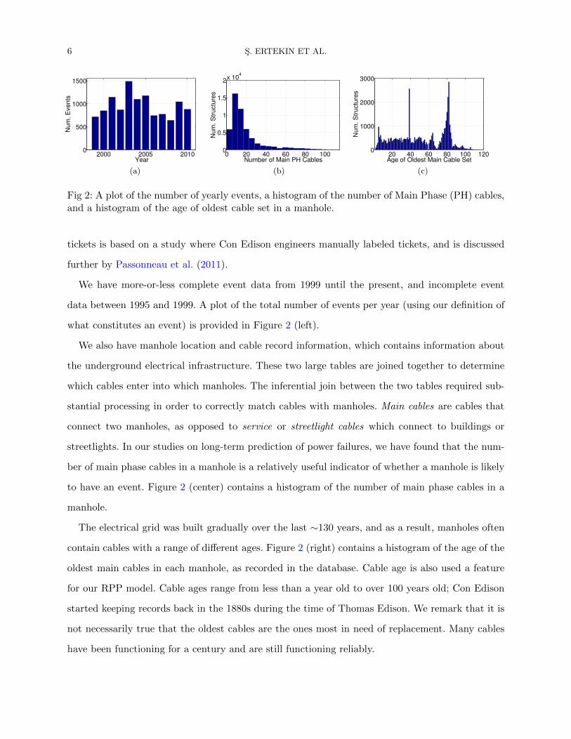
Fig 2: A plot of the number of yearly events, a histogram of the number of Main Phase (PH) cables,and a histogram of the age of oldest cable set in a manhole.

tickets is based on a study where Con Edison engineers manually labeled tickets, and is discussed

further by Passonneau et al. (2011).

We have more-or-less complete event data from 1999 until the present, and incomplete event

data between 1995 and 1999. A plot of the total number of events per year (using our definition of

what constitutes an event) is provided in Figure 2 (left).

We also have manhole location and cable record information, which contains information about

the underground electrical infrastructure. These two large tables are joined together to determine

which cables enter into which manholes. The inferential join between the two tables required sub-

stantial processing in order to correctly match cables with manholes. Main cables are cables that

connect two manholes, as opposed to service or streetlight cables which connect to buildings or

streetlights. In our studies on long-term prediction of power failures, we have found that the num-

ber of main phase cables in a manhole is a relatively useful indicator of whether a manhole is likely

to have an event. Figure 2 (center) contains a histogram of the number of main phase cables in a

manhole.

The electrical grid was built gradually over the last ∼130 years, and as a result, manholes often

contain cables with a range of different ages. Figure 2 (right) contains a histogram of the age of the

oldest main cables in each manhole, as recorded in the database. Cable age is also used a feature

for our RPP model. Cable ages range from less than a year old to over 100 years old; Con Edison

started keeping records back in the 1880s during the time of Thomas Edison. We remark that it is

not necessarily true that the oldest cables are the ones most in need of replacement. Many cables

have been functioning for a century and are still functioning reliably.


200 400 6000

0.5

1

1.5

2

2.5x 10

−3

Number of days

Em

piric

al pro

babili

ty

Empirical probability

Fitted values

(a) Empirical probabilities and fitted values for theself-excitation function g2.

3.81 6.34 8.88 11.42 13.950

1.6

3.2

Sums of empirical probabilities

Em

piric

al pro

babili

ty

Empirical probability

Fitted values

−3x10

x10−4

(b) Empirical probabilities and fitted values for thesaturation function g1.

Fig 3: Fitted functions for empirical probabilities for the Manhattan dataset. These figures displayresults for the conditional frequency estimator used to derive the form of the RPP model. Theleft figure shows the empirical probability of another event given a previous event a given numberof days in the past. The decreasing empirical probability with time motivates our self-excitationfunction. The right plot shows the increase in propensity for another event given the total cumula-tive probability from past events. The curvature indicates that additional events have diminishingreturns on the likelihood of another event, motivating the saturation component of the RPP.

We also have data from Con Edison’s new inspections program. Inspections can be scheduled in

advance, according to a schedule determined by a state mandate. This mandate currently requires

an inspection for each structure at least once every 5 years. Con Edison also performs “ad hoc”

inspections. These occur when a worker is inside a manhole for another purpose (for instance to

connect a new service cable), and chooses to fill in an inspection form. The inspections are broken

down into 5 distinct types, depending on whether repairs are urgent (Level I), or whether the

inspector suggests major infrastructure repairs (Level IV) that are placed on a waiting list to be

completed. Sometimes when continued work is being performed on a single manhole, this manhole

will have many inspections performed within a relatively small amount of time - hence our need

for “diminishing returns” on the influence of an inspection that motivates the saturation function

of the RPP model.

Some questions of interest to power companies are

(i) Can we predict failures continuously in time, and can we model how quickly the influence of

past events and inspections fade over time?

(ii) Can we develop a cost/benefit analysis for proactive maintenance policies?

RPPs will help with both of these questions.

8 S. ERTEKIN ET AL.

3. The Reactive Point Process Model. We begin with a simpler version of RPPs where

there is only one time-series, corresponding to a single entity (manhole). Our data consist of a

series of NE events with event times t1, t2, ..., tNEand a series of given inspection times denoted by

t1, t2, ..., tNI. The inspection times are assumed to be under the control of the experimenter. RPPs

model events as being generated from a non-homogeneous Poisson process with intensity λ(t) where

(1) λ(t) = λ0

1 + g1

∑∀te<t

g2(t− te)

− g3

∑∀ti<t

g4(t− ti)

+ C11[NE≥1]

where te are event times and ti are inspection times. The vulnerability level permanently goes up

by C1 if there is at least one past event, where C1 is a constant that can be fitted. The C11[NE≥1]

term is present to deal with “zero inflation,” where the case of zero events needs to be handled

separately than one or more past events. Functions g2 and g4 are the self-excitation and self-

regulation functions, which have initially large amplitudes and decay over time. Self-exciting point

processes have only g2, and not the other functions, which are novel to RPPs. Functions g1 and g3

are the saturation functions, which start out as the identity function and then flatten farther from

the origin. If the total sum of the excitation terms is large, g1 will prevent the vulnerability level

from increasing too much. Similarly, g4 controls the total possible amount of self-regulation, and

encodes “diminishing returns” for having several inspections in a row.

The RPP model arose based on exploratory work performed using a conditional frequency (CF)

estimator of the data. To construct the CF estimator, we computed the empirical probability

of another event occurring on a day t given that an event occurred at t = 0. To obtain these

probabilities, we first align the sequences of time so that t = 0 represents the time when an event

happened. We now have a series of “trails” that give the probability of another event, conditional

on the last event that occurred for a given manhole. We used only trails that were far apart in

time so we could look at the effect of each event without considering short term influences of other

previous events. What we see from Figure 3(a) is that the conditional probability for experiencing a

second event soon after the first event is high and decays with t. This decay represents self-exciting

behavior. To see evidence of self-excitation from the raw data, we present plots of event times for

several manholes in Figure 4. We see a clear grouping of events which is consistent with self-exciting

behavior. These observations lead us to include the g2 term in (1). The behavior we observe could

not be easily explained using a simple random effects model; an attempt to do this is within Section


Fig 4: Time of events in distinct manholes in the Manhattan data that demonstrate the self-excitating behavior. The x-axis is the number of days elapsed since the day of first record in thedataset and the markers indicate the actual time of events.

4 of the supplementary material.

Next, we evaluate whether subsequent events continue to increase propensity for another event or

whether the risk in the most troubled manholes “saturates” and multiple manhole events in a row

have diminishing-returns on the conditional probabilities. Figure 3(b) shows the saturation effect.

The y-axis of this plot contains raw empirical probabilities of another event. The x-axis are sums

of effects from previous recent events (sums of g2 values). If Figure 3(b) were linear, we would not

see diminishing returns. That is, a linear trend in Figure 3(b) would indicate that each subsequent

event increases the likelihood of another event by the same amount. Instead, we see a distinct curve,

indicating that the additional increase in risk decreases as the number of events rises. To further aid

in developing a functional form of the model, we fit smooth curves to the data displayed in Figures

3(a) and 3(b). The process for fitting these smooth curves, as well as simulation experiments for

validation, is described in detail in the supplementary material. The fitted values for the smooth

curves are:

g2(t) =11.62

1 + e0.039t

g1(t) = 16.98×(

1− log(1 + e−0.15t)× 1

log 2

).

These estimates inspired the parameterizations we provided in Equation (2). We also estimated

the baseline hazard rate λ0 and baseline change C1 for Manhattan as: λ0 = 2.4225 × 10−4 and

C1 = 0.0512.

10 S. ERTEKIN ET AL.

Because the inspection program is relatively new, we were not able to trace out the full functions

g4 and g3; however, we strongly hypothesize that the inspections have an effect that wears off over

time based on a matched pairs study (see, for instance, Passonneau et al., 2011), where we showed

that for manholes that had been inspected at least twice, the second manhole inspection does not

lead to the same reduction in vulnerability as the first manhole inspection does. In what follows,

we will show how the parameters of g1, g2, g3 and g4 can be made to specialize to each individual

manhole adaptively.

Inspired by the CF estimator, we use the family of functions below for fitting power-grid data,

where a1, b1, a3, b3, β, and γ are parameters that can be either modeled or fitted.

g1(ω) = a1 ×(

1− 1

log(2)log(

1 + e−b1ω))

, g2(t) =1

1 + eβt

g3(ω) = a3 ×(

1− 1

log(2)log(

1 + eb3ω))

, g4(t) =−1

1 + eγt.(2)

The factors of log(2) ensure that the vulnerability level is not negative.

We need some notation in order to encode the possibility of multiple manholes. In the case that

there are multiple entities, there are P time-series, each corresponding to a unique entity p. For

medical applications, each p is a patient, for the electrical grid reliability application, p is a manhole.

Our data consist of events {t(p)e}p,e, inspections {t(p)i}p,i, and additionally, we may have covariate

information Mp,j about every entity p, with covariates indexed by j. Covariates for the medical

application might include a patient’s gender, age at the initial time, race, etc. For the manhole

events application, covariates include the number of main phase cables in the manhole (number of

current carrying cables between two manholes), the total number of cable sets (total number of

bundles of cables) including main, service, and streetlight cables, and the age of the oldest cable

set within the manhole. All covariates were normalized to be between -0.5 and 0.5.

Within the Bayesian framework, we can naturally incorporate the covariates to model functions

λp for each p adaptively. Consider β in the expression for the self-excitation function g2 above. The

β terms depend on individual-level covariates. In notation:

(3) g(p)2 (t) =

1

1 + eβ(p)t

, g(p)4 (t) =

−1

1 + eγ(p)t

.

The β(p)’s are assumed to be generated via a hierarchical model of the form

β = log(1 + e−Mυ

), where


υ ∼ N(0, σ2υ)

are the regression coefficients and M is the matrix of observed covariates. The γ(p)’s are modeled

hierarchically in the same manner,

γ = log(1 + e−Mω

),with ω ∼ N(0, σ2

ω).

This permits slower or faster decay of the self-exciting and self-regulating components based on

the characteristics of the individual. For the electrical reliability application, we have noticed that

manholes with more cables and older cables tend to have faster decay of the self-exciting terms for

instance.

Demonstrating the Need for the Saturation Function in the RPP Model. In the previous section

we used exploratory tools on the Manhattan data to demonstrate diminishing returns in risk for

multiple subsequent events. In what follows, we link the exploratory work in the last section with

our modeling framework, demonstrating how the standard linear self-exciting process can produce

unrealistic results under ordinary conditions.

First we show that the self-excitation term can cause the rate of events λ(t) to increase without

bound. To show this, we considered a baseline vulnerability of λ0 = 0.01, setting C1 = 0.1, used

g2(t) = 11+e0.005t

, and omitted the other components of the model (no inspections, no saturation

g1). The self-excitation eventually causes the rate of events to escalate unrealistically as shown in

Figure 5 (upper left). The embedded subfigure is a zoomed-in version of the first 1500 time steps.

When we include the saturation function g1, the excitation is controlled, and the probability of

an event no longer increases to unreasonable levels. We used g1(ω) = 1− 1log 2 log(1 + e−ω), so that

the vulnerability λ(t) can reach to a maximum value of 0.021. The result is in Figure 5 (upper

right).

Now we show the effect of the saturation function g3 in the presence of repeated inspections.

If no manhole events occur and the manhole is repeatedly inspected, then using the linear SEPP

model, its vulnerability levels can become arbitrarily close to 0. This is not difficult to show, and

we do this in Figure 5 (lower left). Here we used λ0 = 0.2, g4(t) = −0.251+e0.002t

, and omitted g3. We

ran the same experiment but with saturation, specifically, with g3(ω) = 1 − 1log 2 log(1 + eω). The

results in Figure 5 (lower right) show that the saturation function never lets the vulnerability drop

unrealistically far below the baseline level.


0 500 1000 1500 2000 25000

0.2

0.4

0.6

0.8

1

Time

λ(t)

500 1000 1500

0.05

0.1

0.15

0.2

(a) Model with self-excitation function g2 (withoutsaturation function g1 and inspections) and a zoomedview of the first 1,500 days.

0 500 1000 1500 2000 2500

0.01

0.015

0.02

0.025

Time

λ(t)

(b) Model with self-excitation function g2 andsaturation function g1 (no inspections).

0 500 1000 1500 2000 25000

0.05

0.1

0.15

0.2

Time

λ(t)

(c) Model with self-regulation function g4 (withoutsaturation function g3 and events).

0 500 1000 1500 2000 25000

0.05

0.1

0.15

0.2

Timeλ(t)

(d) Model with self-regulation function g4 andsaturation function g3 (no events).

Fig 5: The effect of the saturation functions g1 and g3. The dots on the time axis in subfigures (a)and (b) indicate the times of events, and the dots in subfigures (c) and (d) indicate the times ofinspections. The figures on the right include saturation, and the figures on the left do not includesaturation. Without saturation, the self-excitation function in (a) grows unbounded whereas theself-regulation function in (c) drops to an unrealistic level of zero. The effects of the saturationfunctions in Figures (b) and (d) keep g2 and g4 within realistic bounds.

4. Fitting RPP statistical models. In this section we describe our Bayesian framework

for inference using RPP models. The RPP intensity in Equation 1 provides structure to capture

self-excitation, self-regulation, and saturation. First, in Section 4.1 we describe the likelihood for

the RPP statistical model. We then describe prior distributions and our computational strategy

for sampling from the posterior in Section 4.2. Section 4.3 then details the values we use in making

predictions. Along with the results presented here, we extensively evaluated our inference strategy

using a series of simulation experiments, where the goal is to recover parameters of simulated

data for which there is ground truth. We further applied the method of maximum likelihood to

the Manhattan power-grid data. Details of these additional experiments are in the supplementary

material.

4.1. RPP Likelihood. This section describes the likelihood for the RPP statistical model. Using

the intensity function described in Section 3, the RPP likelihood is derived using the likelihood


formula for a non-homogeneous Poisson process over the time interval [0, Tmax]:

(4) logL

({t(p)1 , ...t

(p)

N(p)E

}p

;υ, a1,M

)=

P∑p=1

N(p)E∑e=1

log(λp(t(p)e ))−

∫ Tmax

0λp(u)du

,where υ are coefficients for covariates represented by the matrix M. The covariates are the number

of main phase cables in the manhole (number of current carrying cables between two manholes),

the total number of cable sets (total number of bundles of cables) including main, service, and

streetlight cables, and the age of the oldest cable set within the manhole. All covariates were

normalized to be between -0.5 and 0.5.

4.2. Bayesian RPP. Developing a Bayesian framework facilitates sharing of information be-

tween observably similar manholes, thus making more efficient use of available covariate informa-

tion. The RPP model encodes much of our prior information into the shape of the rate function

given in Equation 1. As discussed in Section 3 we opted for a simple, parsimonious model that

imposes mild regularization and information sharing without adding substantial additional infor-

mation; specifically, we use diffuse Gaussian priors on the log scale for each regression coefficient.

We fit the model using Approximate Bayesian Computation (Diggle and Gratton, 1984). The

principle of Approximate Bayesian Computation (ABC) is to randomly choose proposed parameter

values, use those values to generate data, and then compare the generated data to the observed

data. If the difference is sufficiently small, then we accept the proposed parameters as draws from

the approximate posterior. To do ABC, we need two things: (i) to be able to simulate from the

model and (ii) a summary statistic. To compare the generated and observed data, the summary

statistic from the observed data, S({t(p)1 , ...t(p)

N(p)E

}p), is compared to that of the data simulated from

the proposed parameter values, S({t(p),sim1 , ..., t(p),sim

N(p),simE

}p). If the values are similar, it indicates that

the proposed parameter values may yield a useful model for the data.

A critical difference between updating a parameter value in an ABC iteration versus, for ex-

ample, a Metropolis-Hastings step is that ABC requires simulating from the likelihood whereas

Metropolis-Hastings requires evaluating the likelihood. In our context, we are able to both evaluate

and simulate from the likelihood with approximately the same computational complexity. ABC has

some advantages, namely that we have meaningful summary statistics, discussed below. Further, in

our case it is not particularly computationally challenging, as we already extensively simulate from


the model as a means of evaluating hypothetical inspection policies. We evaluated the adequacy of

this method extensively in simulation studies presented in the supplementary material.

A key conceptual aspect of ABC is that one can choose the summary statistic to best match

the problem. The sufficient statistic for the RPP is the vector of event times, and thus gives no

data reduction - so we choose other statistics. One important insight in constructing our summary

statistic is that changing the parameters in the RPP model alters the distribution of times between

events. The histogram of time differences for a homogenous Poisson Process, for example, has an

exponential decay. The self-exciting process, on the other hand, has a distribution resembling a

lognormal because of the positive association between intensities after an event occurs. Altering

the parameters of the RPP model changes the intensity of self-excitation and self-regulation, thus

altering the distribution of times between events. We construct our first statistic, therefore, by

examining the KL divergence between the distribution of times between events in the data and

the distribution between event times in the simulated data. We do this for each of our proposed

parameters. Examining the distribution of times between events, though not the true sufficient

statistic, captures a concise and low dimensional summary of a key feature of the process. This

statistic does not, however, capture the overall prevalence of events in the process. Since we focus

only on the distribution of times between events, various processes with different overall intensity

could produce distributions with similar KL divergence to the data distribution. We therefore

introduce a second statistic that counts the total number of events. We contend that together these

statistics represent both the spacing and the overall scale (or frequency) of events. Thus, the two

summary measures we use are:

1. DNE: The difference in the number of events in the simulated and observed data.

2. KL: The Kullback-Leibler divergence between two histograms, one from the observed data,

and one from the real data. These are histograms of time differences between events.

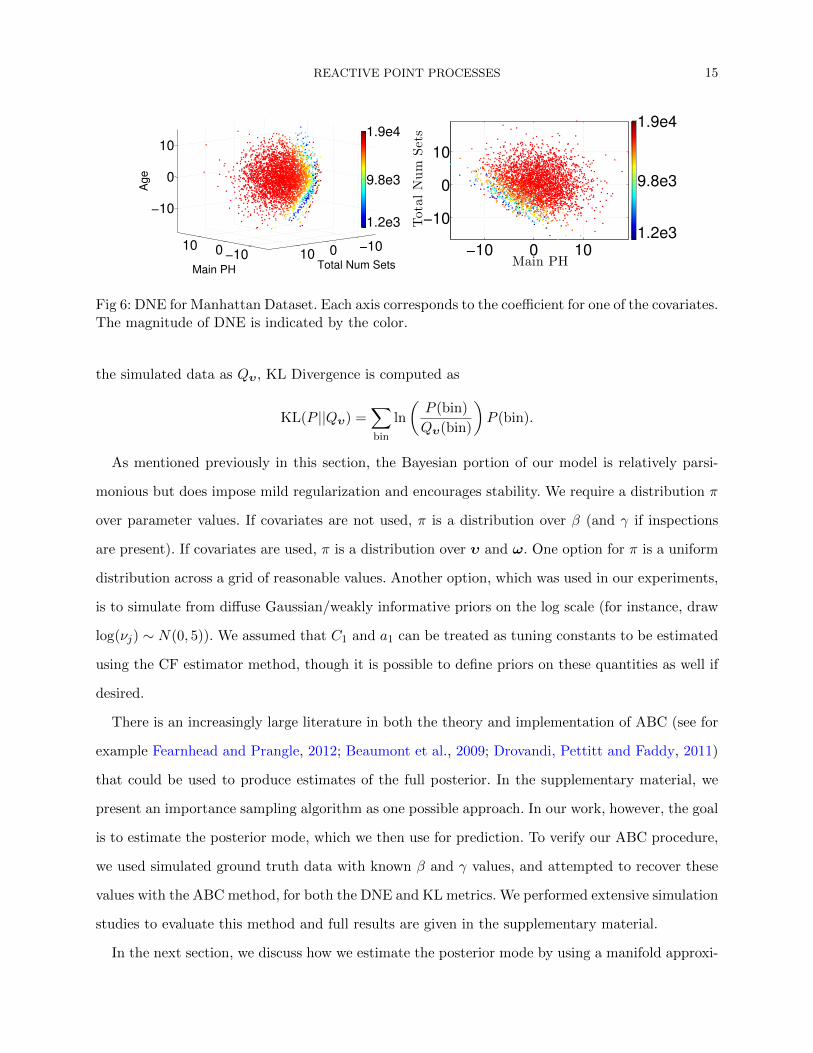
For the NYC data, we visualized three-dimensional parameter values, both for DNE (in Figure

6) and KL (in Figure 7) metrics. In both figures, smaller values (dark blue) are better. As seen, the

regions where KL and DNE are optimized are very similar.

Denoting the probability distribution of the actual data as P and the probability distribution of


−10010 −10010

−10

0

10

Total Num SetsMain PH

Age

1.2e3

9.8e3

1.9e4

−10 0 10

−10

0

10

Main PH

TotalNum

Sets

1.2e3

9.8e3

1.9e4

Fig 6: DNE for Manhattan Dataset. Each axis corresponds to the coefficient for one of the covariates.The magnitude of DNE is indicated by the color.

the simulated data as Qυ, KL Divergence is computed as

KL(P ||Qυ) =∑bin

ln

(P (bin)

Qυ(bin)

)P (bin).

As mentioned previously in this section, the Bayesian portion of our model is relatively parsi-

monious but does impose mild regularization and encourages stability. We require a distribution π

over parameter values. If covariates are not used, π is a distribution over β (and γ if inspections

are present). If covariates are used, π is a distribution over υ and ω. One option for π is a uniform

distribution across a grid of reasonable values. Another option, which was used in our experiments,

is to simulate from diffuse Gaussian/weakly informative priors on the log scale (for instance, draw

log(νj) ∼ N(0, 5)). We assumed that C1 and a1 can be treated as tuning constants to be estimated

using the CF estimator method, though it is possible to define priors on these quantities as well if

desired.

There is an increasingly large literature in both the theory and implementation of ABC (see for

example Fearnhead and Prangle, 2012; Beaumont et al., 2009; Drovandi, Pettitt and Faddy, 2011)

that could be used to produce estimates of the full posterior. In the supplementary material, we

present an importance sampling algorithm as one possible approach. In our work, however, the goal

is to estimate the posterior mode, which we then use for prediction. To verify our ABC procedure,

we used simulated ground truth data with known β and γ values, and attempted to recover these

values with the ABC method, for both the DNE and KL metrics. We performed extensive simulation

studies to evaluate this method and full results are given in the supplementary material.

In the next section, we discuss how we estimate the posterior mode by using a manifold approxi-


−100

10 −20−10010

−10

0

10

20

Total Num SetsMain PH

Age

0.13

0.31

0.48

−10 0 10−20

−10

0

10

Main PH

TotalNum

Sets

0.13

0.31

0.48

Fig 7: KL for Manhattan Dataset. Each axis corresponds to the coefficient for one of the covariates.The magnitude of KL is indicated by the color.

mation to the region of high posterior density. We begin by generating a set of proposed parameter

values using the prior distributions. Consistent with ABC, we simulate data from each set of candi-

date values and compare the simulated data to our observed data using the KL and DNE statistics

described above. (From here, we could, for example, define a kernel and accept draws with a given

probability as in importance sampling. Instead, our goal is estimating the posterior mode to find

parameters for the policy decision, as we describe next.)

4.3. Choosing Parameter Values for the Policy Decision. For the policy simulation in Section

6 we wish to choose one set of parameter values to inform our decision. In order to choose a single

best value of the parameters, we fit a polynomial manifold to the intersection of the bottom 10%

of KL values and the bottom 10% of DNE values. Defining υ1, υ2 and υ3 as the coefficients for

number of main phase cables, age of oldest main cable set and total number of sets features, the

formula for the manifold is:

υ3 = −9.6− 0.98υ1 − 0.13υ2 − 1.1× 10−3(υ1)2 − 3.6× 10−3υ1υ2 + 4.67× 10−2(υ2)2,

which is determined by a least squares fit to the data. The fitted manifold is shown in Figure 8

along with the data.

We then optimized for the point on the manifold closest to the origin. This implicitly adds

regularization, as it chooses the parameter values closest to the origin. This point is υ1 = −4.6554,

υ2 = −0.5716, and υ3 = −4.8028.

Note that cable age (corresponding to the second coefficient) is not the most important feature

defining the manifold. As previous studies have shown (Rudin et al., 2010), even though there are


−15−10

−50

5−10

010

−20

0

20

AgeMain PHT

ota

l N

um

Sets

Fig 8: Fitted manifold of υ values with smallest KL divergence and smallest DNE.

very old cables in the city, the age of cables within a manhole is not alone the best predictor of

vulnerability. Now we also know that it is not the best predictor of the rate of decay of vulner-

ability back to baseline levels. This supports Con Edison’s goal to prioritize the most vulnerable

components of the power-grid, rather than simply replacing the oldest components. The features

that mainly determine decay of the self-excitation function g2 are the number of main phase cables

and the number of cable sets. As either or both of these numbers increase, decay rate β increases,

meaning that manholes with more cables tend to return to baseline levels faster than manholes

with fewer cables.

5. Predicting events on the NYC power-grid. Our first experiment aims to evaluate

whether the CF estimator or the feature-based strategy introduced above is better in terms of

identifying the most vulnerable manholes. To do this, we selected 5,000 manholes (rank 1,001-6,000

from the project’s current long-term prediction model). These manholes have similar vulnerability

levels, which allows us to isolate the self-exciting effect without modeling the baseline level. Using

both the feature-based β (ABC, with KL metric) and constant β (CF estimator method) strategies,

the models were trained on data through 2009, and then we estimated the vulnerabilities of the

manholes on December 31st, 2009. These vulnerabilities were used as the initial vulnerabilities for

an evaluation on the 2010 event data. 2010 is a relevant year because the first inspection cycle

ended in 2009. All manholes had been inspected at least once, and many were inspected towards

the end of 2009, which stabilizes the inspection effects. For each of the 53K manholes and at each

of the 365 days of 2010, when we observed a serious event in a manhole p, we evaluated the rank

of that manhole with respect to both the feature-based and non-feature-based models, where rank


Fig 9: Ranking differences between feature-based and constant (non-feature-based) β strategies.

0 100 200 300 4000

100

200

300

Days

Ra

nk

Constant βFeature-based β

represents the number of manholes that were given higher vulnerabilities than manhole p. As our

goal is to compare the relative rankings provided by the two strategies, we consider only events

where the vulnerabilities assigned by both strategies are different than the baseline vulnerability.

Figure 9 displays the ranks of the manholes on the day of their serious event. A smaller rank

indicates being higher up the list, thus lower is better. Overall, we find that the feature-based β

strategy performs better than the non-feature-based strategy over all of the rank comparisons in

2010 (pvalue .09, sign test). Our results mainly illustrate that using different decay rates on past

events for different types of manholes leads to better predictions. Recall from Section 4.3 that larger

manholes tend to recover faster from previous events. The approach without the features ignores

the differences between manholes, and uses the same decay rate, whereas the feature-based RPP

takes these decay rates into account in making predictions.

In the second experiment, we compared the feature-based β strategy to the Cox Proportional-

Hazard Model, which is commonly used in survival analysis to assess the probability of failure in

mechanical systems. We employed this model to assess the likelihood of a manhole having a serious

event on a particular day. For each manhole, we used the same three static covariates as in the

feature-based β model, and developed four time-dependent features. The time-varying features for

day t are 1) the number of times the manhole was a trouble hole (source of the problem) for a serious

event until t, 2) the number of times the manhole was a trouble hole for a serious event in the last

year, 3) the number of times the manhole was a trouble hole for a precursor event (less serious


event) until t, and 4) the number of times the manhole was a trouble hole for a precursor event

in the last year. The feature-based β model currently does not differentiate serious and precursor

events, though it is a direct extension to do this if desired. The model was trained using the coxph

function in the R survival package using data prior to 2009, and then predictions were made on the

test set of 5,000 manholes in the 2010 dataset. These predictions were transformed into ranked lists

of manholes for each day. We then compared the ranks achieved by the Cox model with the ranks

of manholes at the time of events. The difference of aggregate ranks was in favor of the feature-

based β approach (pvalue 7e-06, sign test), indicating that the feature-based β strategy provides a

substantial advantage in its ability to prioritize vulnerable manholes.

The Cox model we compared with represents a “long-term” model similar to what we were using

previously for manhole event prediction on Con Edison data (Rudin et al., 2010). The Cox model

considers different information, namely counts of past events. These counts are time-varying, but

the past events do not smoothly wear off in time as they do for the RPP. The fact that the RPP

model is competitive with the Cox model indicates that the effects of past manhole events do wear

off with time (in agreement with Figure 3 where we traced the decay directly using data). The

saturating elements of the model ensure that the model is physically plausible, since as we showed

in Section 3 that the results could be unphysical (with rates going to 0 or above 1) without the

saturation.

6. Making Broader Policy Decisions Using RPPs. Because the RPP model is a gener-

ative model, it can be used to simulate the future, and thus assist with broader policy decisions

regarding how often inspections should be performed. This can be used to justify allocation of

spending. Con Edison’s existing inspection policy is a combination of targeted periodic inspections

and ad-hoc inspections. The targeted inspections are planned in advance, whereas the ad hoc in-

spections are unscheduled. An ad hoc inspection could be performed while a utility worker is in

the process of, for instance, installing new service cable to a building or repairing an outage. Either

source of inspection can result in an urgent repair (Type I), an important but not urgent repair

(Type II), a suggested structural repair (Types III and IV), or no repair, or any combination of

repairs. Urgent repairs need to be completed before the inspector leaves the manhole, whereas Type

IV repairs are placed on a waiting list. According to the current inspections policy, each manhole


undergoes a targeted inspection every 5 years. The choice of inspection policy to simulate can be

determined very flexibly, and any inspection policy and hypothesized effect of inspections can be

examined through simulation.

As a demonstration, we conducted a simulation over a 20 year future time horizon that permits

a cost-benefit analysis of the inspection program, when targeted inspections are performed at a

given frequency. To do this simulation we require the following:

• A characterization of manhole vulnerability. For Manhattan, this is learned from the past

using the ABC RPP feature-based β training strategy for the saturation function g1 and the

self-excitation function g2 discussed above. Saturation and self-regulation functions g3 and

g4 for the inspection program cannot yet be learned due to the newness of the inspection

program and are discussed below.

• An inspection policy. The policy can include targeted, ad hoc, or history-based inspections.

We chose to evaluate “bright line” inspection policies, where each manhole is inspected once

in each Y year period, where Y is varied (discussed below). We also included an ad hoc

inspection policy that visits 3 manholes per day on average.

Effect of Inspections: The effect of inspections on the overall vulnerability of manholes were

designed in consultation with domain experts. The choices are somewhat conservative, so as to give

a lower bound for costs. The effect of an urgent repair (Type I) is different from the effect of less

urgent repairs (Types II, III, and IV). For all inspection types, after 1 year beyond the time of the

inspection, the effect of the inspection decays to, on average, 85% of its initial effect, in agreement

with a short-term empirical study on inspections. (There is some uncertainty in this initial effect,

and the initial drop in vulnerability is chosen from a normal distribution so that after one year,

the effect decays to a mean of 85%.) For Type I inspections, the effect of the inspection decays to

baseline levels after approximately 3000 days, and for Type II, III, and IV, which are more extensive

repairs, the effect fully decays after 7000 days. In particular, we use the following g4 functions:

gTypeI4 (t) = −83.7989× (r × 5× 10−4 + 3.5× 10−3)× 1

1 + e0.0018t(5)

gTypeII,III,IV4 (t) = −49.014× (r × 5× 10−4 + 7× 10−3)× 1

1 + e0.00068t(6)

where r is randomly sampled from a standard normal distribution. For all inspection types, we


0 2000 4000 6000 8000−0.4

−0.3

−0.2

−0.1

0

(a) g4 for Type I inspections.

0 2000 4000 6000 8000−0.4

−0.3

−0.2

−0.1

0

(b) g4 for Type II, III, IV.

−1 −0.75 −0.5 −0.25 00

0.25

0.5

0.75

1

(c) g3 = 0.4(

1 − log(1 + e3.75x) 1log 2

)Fig 10: Saturation and self-regulation functions g3 and g4 for simulation.

used the following g3 saturation function:

g3(t) = 0.4×(

1− log(1 + e−3.75t)× 1

log 2

)which ensures that subsequent inspections do not lower the vulnerability to more than 60% of the

baseline vulnerability. Sampled g4 functions for Type I and Type II, II, IV, along with g3 are shown

in Figure 10.

One targeted inspection per manhole was distributed randomly across Y years for the bright

line Y -year inspection policies, and 3×365 =1095 ad-hoc inspections for each year were uniformly

distributed, which corresponds to 3 ad-hoc inspections per day for the whole power-grid on average.

During the simulation, when we arrived at a time step with an inspection, the inspection outcome

was Type I with 25% probability, or one of Types II, III, or IV, with 25% probability. In the

rest of cases (50% probability), the inspection was clean, and the manhole’s vulnerability was

not affected by the inspection. If the inspection resulted in a repair, we sampled r randomly and

randomly chose the inspection outcome (Type I or Types II, III, IV). This percentage breakdown

was observed approximately for a recent year of inspections in NYC.

To initialize manhole vulnerabilities for a bright line policy of Y years, we simulated the previous

Y -year inspection cycle, and started the simulation with the vulnerabilities obtained at the end of

this full cycle.

Simulation Results: We simulated events and inspections for 53.5K manholes for bright line

policies ranging from Y = 1 year to Y = 20 years. Naturally, a longer inspection cycle corresponds

to fewer daily inspections, which translates into an increase in overall vulnerabilities and an increase

in the number of events. This is quantified in Figure 11, which shows the projected number of

inspections and events for each Y year bright line policy. If we change from a 6 year bright line


0 5 10 15 200

5

10

x 105

Inspection Frequency in Years

Nu

mb

er

of

Insp

ectio

ns

0 5 10 15 208

9

10

11x 104

Inspection Frequency in Years

Nu

mb

er

of

Eve

nts

Fig 11: Number of events and inspections based on bright line policy. Number of years Y for thebright line policy is on the horizontal axis in both figures. The left figure shows the number ofinspections, the right figure shows the number of events.

inspection policy to a 4 year policy, we estimate a reduction of approximately 100 events per year.

The relative costs of inspections and events can thus be considered in order to justify a particular

choice of Y for the bright line policy.

Let us say, for instance, that each inspection costs CI and each event costs CE . The simulation

results allow us to denote the forecasted expected number of events over a period of time T as

a function of the inspection frequency Y , which we denote by NE(Y, T ). The value of NE(Y, T )

comes directly from the simulation, as plotted in Figure 11. Let us make a decision for Y for P

total manholes, over a period of time T . To do this, we would choose a Y that minimizes the total

cost

CE ×NE(Y, T ) + CI × P × T/Y.

This line of reasoning provides a quantitative mechanism for decision making and can be used to

justify a particular choice of inspection policy.

7. Conclusion. Keeping our electrical infrastructure safe and reliable is of critical concern, as

power outages affect almost all aspects of our society including hospitals, financial centers, data

centers, transportation, and supermarkets. If we are able to combine historical data with the best

available statistical tools, it will be possible to impact our ability to maintain an ever aging and

growing power-grid. In this work, we presented a methodology for modeling power-grid failures

that is based on natural assumptions: (i) that power failures have a self-exciting property, which

was hypothesized by Con Edison engineers, (ii) that the power company’s actions are able to

regulate vulnerability levels, (iii) that the effects on the vulnerability level of past events or repairs

can saturate, and (iv) that vulnerability estimates should be similar between similar entities. We


have been able to show directly (using the CF estimator for the RPP) that the self-exciting and

saturation assumptions hold. We demonstrated through experiments on past power-grid data from

NYC, and through simulations, that the RPP model is able to capture the relevant dynamics well

enough to predict power failures better than the current approaches in use.

The modeling assumptions that underlie RPPs can be directly ported to other problems. RPPs

are a natural fit for problems in healthcare, where medical conditions cause self-excitation, and

treatments provide regulation. Through the Bayesian framework we introduced, RPPs extend to

a broad range of problems where predictive power can be pooled among multiple related entities,

whether manholes or medical patients.

The results presented in this work show for the first time that manhole events can be predicted

in the short term, which was previously thought not to be possible. Knowing how one might

do this permits us to take preventive action to keep vulnerability levels low, and can help make

broader policy decisions for power-grid maintenance through simulation of many uncertain futures,

simulated over any desired policy.

Acknowledgements. Funding for this work provided by Con Edison and National Science

Foundation CAREER grant IIS-1053407 to C. Rudin.

References.

Aıt-Sahalia, Y., Cacho-Diaz, J. and Laeven, R. J. (2010). Modeling financial contagion using mutually exciting

jump processes Technical Report, National Bureau of Economic Research.

Bacry, E., Delattre, S., Hoffmann, M. and Muzy, J. (2013). Modelling microstructure noise with mutually

exciting point processes. Quantitative Finance 13 65–77.

Bartlett, M. (1963). The spectral analysis of point processes. Journal of the Royal Statistical Society. Series B

(Methodological) 25 264–296.

Beaumont, M. A., Cornuet, J.-M., Marin, J.-M. and Robert, C. P. (2009). Adaptive approximate Bayesian

computation. Biometrika 96 983–990.

Blundell, C., Beck, J. and Heller, K. A. (2012). Modelling Reciprocating Relationships with Hawkes Processes.

Advances in Neural Information Processing Systems 1–9.

Chehrazi, N. and Weber, T. A. (2011). Dynamic Valuation of Delinquent Credit-Card Accounts. Working Paper.

Crane, R. and Sornette, D. (2008). Robust dynamic classes revealed by measuring the response function of a

social system. Proceedings of the National Academy of Sciences 105 15649–15653.

Diggle, P. J. and Gratton, R. J. (1984). Monte Carlo methods of inference for implicit statistical models. Journal

of the Royal Statistical Society. Series B 46 193–227.


DOE (2008). The Smart Grid, An Introduction Technical Report. Prepared by Litos Strategic Communication. US

Department of Energy, Office of Electricity Delivery & Energy Reliability.

Drovandi, C. C., Pettitt, A. N. and Faddy, M. J. (2011). Approximate Bayesian computation using indirect

inference. Journal of the Royal Statistical Society: Series C (Applied Statistics) 60 317–337.

Du, N., Song, L., Woo, H. and Zha, H. (2013). Uncover Topic-Sensitive Information Diffusion Networks.

Egesdal, M., Fathauer, C., Louie, K., Neuman, J., Mohler, G. and Lewis, E. (2010). Statistical and stochastic

modeling of gang rivalries in Los Angeles. SIAM Undergraduate Research Online 3 72–94.

Embrechts, P., Liniger, T. and Lin, L. (2011). Multivariate Hawkes processes: an application to financial data.

Journal of Applied Probability 48A 367–378.

Ertekin, S., Rudin, C. and McCormick, T. (2013). Predicting Power Failures with Reactive Point Processes. In

AAAI Workshop on Late-Breaking Developments.

Fearnhead, P. and Prangle, D. (2012). Constructing summary statistics for approximate Bayesian computation:

semi-automatic approximate Bayesian computation. Journal of the Royal Statistical Society: Series B (Statistical

Methodology) 74 419–474.

Filimonov, V. and Sornette, D. (2012). Quantifying reflexivity in financial markets: Toward a prediction of flash

crashes. Physical Review E 85 056108.

Guttorp, P. and Thorarinsdottir, T. L. (2012). Bayesian Inference for Non-Markovian Point Processes. In

Advances and Challenges in Space-time Modeling of Natural Events, (E. Porcu, J. Montero and M. Schlather,

eds.). Lecture Notes in Statistics 79-102. Springer Berlin Heidelberg.

Hardiman, S. J., Bercot, N. and Bouchaud, J.-P. (2013). Critical reflexivity in financial markets: a Hawkes

process analysis. The European Physical Journal B 86 1-9.

Johnson, D. H. (1996). Point process models of single-neuron discharges. Journal of computational neuroscience 3

275–299.

Kerstan, J. (1964). Teilprozesse Poissonscher Prozesse. Transactions of the Third Prague Conference on Information

Theory, Statistical Decision Functions and Random Processes 377–403.

Krumin, M., Reutsky, I. and Shoham, S. (2010). Correlation-based analysis and generation of multiple spike trains

using Hawkes models with an exogenous input. Frontiers in computational neuroscience 4.

Lewis, E., Mohler, G., Brantingham, P. J. and Bertozzi, A. (2010). Self-exciting point process models of

insurgency in Iraq. UCLA CAM Reports 10 38.

Louie, K., Masaki, M. and Allenby, M. (2010). A Point Process Model for Simulating Gang-on-Gang Violence

Technical Report, UCLA.

Masuda, N., Takaguchi, T., Sato, N. and Yano, K. (2012). Self-exciting point process modeling of conversation

event sequences. arXiv preprint arXiv:1205.5109.

Mitchell, L. and Cates, M. E. (2009). Hawkes process as a model of social interactions: a view on video dynamics.

Journal of Physics A: Mathematical and Theoretical 43 045101.

Mohler, G., Short, M., Brantingham, P., Schoenberg, F. and Tita, G. (2011). Self-exciting point process

modeling of crime. Journal of the American Statistical Association 106 100–108.


NYBC (2010). Electricity OUTLOOK: Powering New York City’s Economic Future Technical Report. New York

Building Congress Reports: Energy Outlook 2010-2025.

Ogata, Y. (1988). Statistical Models for Earthquake Occurrences and Residual Analysis for Point Processes. Journal

of the American Statistical Association 83 9–27.

Ogata, Y. (1998). Space-time point-process models for earthquake occurrences. Annals of the Institute of Statistical

Mathematics 50 379–402.

Passonneau, R., Rudin, C., Radeva, A., Tomar, A. and Xie, B. (2011). Treatment Effect of Repairs to an

Electrical Grid: Leveraging a Machine Learned Model of Structure Vulnerability. In Proceedings of the KDD

Workshop on Data Mining Applications in Sustainability (SustKDD), 17th Annual ACM SIGKDD Conference on

Knowledge Discovery and Data Mining.

Peruggia, M. and Santner, T. (1996). Bayesian analysis of time evolution of earthquakes. Journal of the American

Statistical Association 1209–1218.

Reynaud-Bouret, P. and Schbath, S. (2010). Adaptive estimation for Hawkes processes; application to genome

analysis. The Annals of Statistics 38 2781–2822.

Rhodes, L. (2013). US Power Grid Has Issues with Reliability. Data Center Knowledge (www.datacenterknowledge.

com): Industry Perspectives.

Rudin, C., Passonneau, R., Radeva, A., Dutta, H., Ierome, S. and Isaac, D. (2010). A Process for Predicting

Manhole Events In Manhattan. Machine Learning 80 1–31.

Rudin, C., Waltz, D., Anderson, R. N., Boulanger, A., Salleb-Aouissi, A., Chow, M., Dutta, H., Gross, P.,

Huang, B., Ierome, S., Isaac, D., Kressner, A., Passonneau, R. J., Radeva, A. and Wu, L. (2012). Machine

Learning for the New York City Power Grid. IEEE Transactions on Pattern Analysis and Machine Intelligence

34 328–345.

Rudin, C., Ertekin, S., Passonneau, R., Radeva, A., Tomar, A., Xie, B., Lewis, S., Riddle, M., Pangsriv-

inij, D. and McCormick, T. (2014). Analytics for Power Grid Distribution Reliability in New York City. Inter-

faces. To appear.

Simma, A. and Jordan, M. I. (2010). Modeling Events with Cascades of Poisson Processes. In Proc. of the 26th

Conference on Uncertainty in Artificial Intelligence (UAI2010).

So, H. (2004). Council approves bill on Con Ed annual inspections. The Villager, Volume 74, Number 23.

Taddy, M. A. and Kottas, A. (2012). Mixture Modeling for Marked Poisson Processes. Bayesian Analysis 7 335–

362.

S. Ertekin and C. Rudin

MIT Sloan School of Management

Massachusetts Institute of Technology

Cambridge, MA 02139

E-mail: [email protected]

[email protected]

T. H. McCormick

Department of Statistics

University of Washington

Seattle, WA 98195

E-mail: [email protected]

www.datacenterknowledge.com

www.datacenterknowledge.com

mailto:[email protected]



reactive point processes: a new approach to predicting ...tylermc/pubs/mccormick_manhole.pdf ·...

Documents