445_designing reactive distillation processes with improved
TRANSCRIPT
Designing Reactive Distillation
Processes with Improved Efficiency
economy, exergy loss and responsiveness


Designing Reactive Distillation
Processes with Improved Efficiency
economy, exergy loss and responsiveness
Proefschrift
ter verkrijging van de graad van doctoraan de Technische Universiteit Delft,
op gezag van de Rector Magnificus prof. dr. ir. J. T. Fokkema,voorzitter van het College voor Promoties,
in het openbaar te verdedigen op maandag 14 november 2005 om 13:00 uurdoor
Cristhian Paul ALMEIDA-RIVERA
Ingeniero Quımico(Escuela Politecnica Nacional, Ecuador)
Scheikundig ingenieurgeboren te Quito, Ecuador

Dit proefschrift is goedgekeurd door de promotor:Prof. ir. J. Grievink
Samenstelling promotiecommissie:
Rector Magnificus VoorzitterProf. ir. J. Grievink Technische Universiteit Delft, promotorProf. dr. G. Frens Technische Universiteit DelftProf. ir. G. J. Harmsen Technische Universiteit Delft/Shell ChemicalsProf. dr. F. Kapteijn Technische Universiteit DelftProf. dr. ir. H. van den Berg Twente Universiteitdr. A. C. Dimian Universiteit van AmsterdamProf. dr. ir. A. I. Stankiewicz Technische Universiteit Delft/DSMProf. dr. ir. P. J. Jansens Technische Universiteit Delft (reserve lid)
Copyright c© 2005 by Cristhian P. Almeida-Rivera, Delft
All rights reserved. No part of the material protected by this copyright notice may be reproduced
or utilized in any form or by any means, electronic or mechanical, including photocopying, recording
or by any information storage and retrieval system, without written permission from the author. An
electronic version of this thesis is available at http://www.library.tudelft.nl
Published by Cristhian P. Almeida-Rivera, Delft
ISBN 9-090200-37-1 / 9789090200378
Keywords: process systems engineering, reactive distillation, conceptual process design, multiechelon
design approach, life-span inspired design methodology, residue curve mapping, multilevel approach,
dynamic optimization, singularity theory, dynamic simulation, non-equilibrium thermodynamics, ex-
ergy, responsiveness
Printed by PrintPartners Ipskamp in the Netherlands

Dedicated tomy daughter Lucıa and
my wife Paty


Contents
1 Introduction 1
1.1 A Changing Environment for the Chemical Process Industry . . . . . . 2
1.2 Reactive Distillation Potential . . . . . . . . . . . . . . . . . . . . . . . . 3
1.3 Significance of Conceptual Design in Process Systems Engineering . . . 5
1.4 Scope of Research . . . . . . . . . . . . . . . . . . . . . . . . . . . . . . 9
1.5 Outline and Scientific Novelty of the Thesis . . . . . . . . . . . . . . . . 11
2 Fundamentals of Reactive Distillation 13
2.1 Introduction . . . . . . . . . . . . . . . . . . . . . . . . . . . . . . . . . . 14
2.2 One-stage Level: Physical and Chemical (non-) Equilibrium . . . . . . . 16
2.3 Multi-stage Level: Combined Effect of Phase and Chemical Equilibrium 17
2.4 Multi-stage Level: Reactive Azeotropy . . . . . . . . . . . . . . . . . . . 20
2.5 Non-equilibrium Conditions and Rate Processes . . . . . . . . . . . . . . 23
2.6 Distributed Level: Column Structures . . . . . . . . . . . . . . . . . . . 26
2.7 Distributed Level: Hydrodynamics . . . . . . . . . . . . . . . . . . . . . 29
2.8 Flowsheet Level: Units and Connectivities . . . . . . . . . . . . . . . . . 30
2.9 Flowsheet Level: Steady-State Multiplicities . . . . . . . . . . . . . . . . 31
2.10 Summary of Design Decision Variables . . . . . . . . . . . . . . . . . . . 38
3 Conceptual Design of Reactive Distillation Processes: A Review 41
3.1 Introduction . . . . . . . . . . . . . . . . . . . . . . . . . . . . . . . . . . 42
3.2 Graphical Methods . . . . . . . . . . . . . . . . . . . . . . . . . . . . . . 42
3.3 Optimization-Based Methods . . . . . . . . . . . . . . . . . . . . . . . . 61
3.4 Evolutionary/Heuristic Methods . . . . . . . . . . . . . . . . . . . . . . 65
3.5 Concluding Remarks . . . . . . . . . . . . . . . . . . . . . . . . . . . . . 70
i

Contents
4 A New Approach in the Conceptual Design of RD Processes 75
4.1 Introduction . . . . . . . . . . . . . . . . . . . . . . . . . . . . . . . . . . 76
4.2 Interactions between Process Development and Process Design . . . . . 77
4.3 Structure of the Design Process . . . . . . . . . . . . . . . . . . . . . . . 79
4.4 Life-Span Performance Criteria . . . . . . . . . . . . . . . . . . . . . . . 82
4.5 Multiechelon Approach: The Framework of the Integrated Design Method-ology . . . . . . . . . . . . . . . . . . . . . . . . . . . . . . . . . . . . . . 84
4.6 Concluding Remarks . . . . . . . . . . . . . . . . . . . . . . . . . . . . . 87
5 Feasibility Analysis and Sequencing: A Residue Curve Mapping Ap-proach 89
5.1 Introduction . . . . . . . . . . . . . . . . . . . . . . . . . . . . . . . . . . 90
5.2 Input-Output Information Flow . . . . . . . . . . . . . . . . . . . . . . . 90
5.3 Residue Curve Mapping Technique . . . . . . . . . . . . . . . . . . . . . 91
5.4 Feasibility Analysis: An RCM-Based Approach . . . . . . . . . . . . . . 95
5.5 Case Study: Synthesis of MTBE . . . . . . . . . . . . . . . . . . . . . . 97
5.6 Concluding Remarks . . . . . . . . . . . . . . . . . . . . . . . . . . . . . 103
6 Spatial and Control Structure Design in Reactive Distillation 107
6.1 Multilevel Modeling . . . . . . . . . . . . . . . . . . . . . . . . . . . . . 108
6.2 Simultaneous Optimization of Spatial and Control Structures in ReactiveDistillation . . . . . . . . . . . . . . . . . . . . . . . . . . . . . . . . . . 115
6.3 Concluding Remarks . . . . . . . . . . . . . . . . . . . . . . . . . . . . . 124
7 Steady and Dynamic Behavioral Analysis 127
7.1 Introduction . . . . . . . . . . . . . . . . . . . . . . . . . . . . . . . . . . 128
7.2 Steady-State Behavior . . . . . . . . . . . . . . . . . . . . . . . . . . . . 129
7.3 Dynamic Behavior . . . . . . . . . . . . . . . . . . . . . . . . . . . . . . 144
7.4 Concluding Remarks . . . . . . . . . . . . . . . . . . . . . . . . . . . . . 152
ii

Contents
8 A Design Approach Based on Irreversibility 155
8.1 Introduction . . . . . . . . . . . . . . . . . . . . . . . . . . . . . . . . . . 156
8.2 Generic Lumped Reactive Distillation Volume Element . . . . . . . . . . 158
8.3 Integration of Volume Elements to a Column Structure . . . . . . . . . . 168
8.4 Application 1. Steady-state Entropy Production Profile in a MTBE Re-active Distillation Column . . . . . . . . . . . . . . . . . . . . . . . . . . 178
8.5 Application 2. Bi-Objective Optimization of a MTBE Reactive Distilla-tion Column . . . . . . . . . . . . . . . . . . . . . . . . . . . . . . . . . . 181
8.6 Application 3. Tri-Objective Optimization of a MTBE Reactive Distil-lation Column: A Sensitivity-Based Approach . . . . . . . . . . . . . . . 185
8.7 Comparison Between Classical and Green Designs . . . . . . . . . . . . 189
8.8 Concluding Remarks . . . . . . . . . . . . . . . . . . . . . . . . . . . . . 191
9 Conclusions and Outlook 193
9.1 Introduction . . . . . . . . . . . . . . . . . . . . . . . . . . . . . . . . . . 194
9.2 Conclusions Regarding Specific Scientific Design Questions . . . . . . . . 194
9.3 Conclusions Regarding Goal-Oriented Questions . . . . . . . . . . . . . 200
9.4 Scientific Novelty of this Work . . . . . . . . . . . . . . . . . . . . . . . 201
9.5 Outlook and Further Research . . . . . . . . . . . . . . . . . . . . . . . 205
A Model Description and D.O.F. Analysis of a RD Unit 209
A.1 Mathematical Models . . . . . . . . . . . . . . . . . . . . . . . . . . . . 209
A.2 Degree of Freedom Analysis . . . . . . . . . . . . . . . . . . . . . . . . . 217
B Synthesis of MTBE: Features of the System 221
B.1 Motivation . . . . . . . . . . . . . . . . . . . . . . . . . . . . . . . . . . 221
B.2 Description of the System . . . . . . . . . . . . . . . . . . . . . . . . . . 222
B.3 Thermodynamic Model . . . . . . . . . . . . . . . . . . . . . . . . . . . 224
B.4 Physical Properties, Reaction Equilibrium and Kinetics . . . . . . . . . 224
References 230
Summary 247
iii

Contents
Sammenvatting 251
Acknowledgements 257
Publications 261
About the author 263
Index 265
List of Symbols 267
Colophon 277
iv

List of Figures
1.1 Schematic representation of the conventional and highly task-integratedRD unit for the synthesis of methyl acetate . . . . . . . . . . . . . . . . 3
2.1 Schematic representation of the relevant spatial scales in reactive distil-lation . . . . . . . . . . . . . . . . . . . . . . . . . . . . . . . . . . . . . 14
2.2 Representation of stoichiometric and reactive distillation lines . . . . . . 19
2.3 Graphical determination of reactive azeotropy . . . . . . . . . . . . . . . 21
2.4 Phase diagram for methanol in the synthesis of MTBE expressed in termsof transformed compositions . . . . . . . . . . . . . . . . . . . . . . . . . 23
2.5 Schematic representation of the Film Model . . . . . . . . . . . . . . . . 26
2.6 Separation train for an homogeneous catalyst . . . . . . . . . . . . . . . 27
2.7 Key design decision variables in RD . . . . . . . . . . . . . . . . . . . . 39
3.1 Method of statics analysis . . . . . . . . . . . . . . . . . . . . . . . . . . 43
3.2 Procedure for the construction of attainable region . . . . . . . . . . . . 48
3.3 Dimension reduction through transformed compositions . . . . . . . . . 50
3.4 Procedure for sketching the McCabe-Thiele diagram for an isomerizationreaction . . . . . . . . . . . . . . . . . . . . . . . . . . . . . . . . . . . . 57
3.5 Schematic representation of the phenomena vectors in the compositionspace. . . . . . . . . . . . . . . . . . . . . . . . . . . . . . . . . . . . . . 58
3.6 Influence of feed location on reactant conversion . . . . . . . . . . . . . 67
3.7 Column internals’ driven design: ideal reactor-separator train . . . . . . 68
3.8 Relation between conversion and reflux ratio . . . . . . . . . . . . . . . 68
3.9 Procedure to estimate reactive zone height, reflux ratio and column di-ameter . . . . . . . . . . . . . . . . . . . . . . . . . . . . . . . . . . . . . 69
v

List of Figures
4.1 The design problem regarded as the combination of a design programand a development program. . . . . . . . . . . . . . . . . . . . . . . . . 78
4.2 Overall design problem . . . . . . . . . . . . . . . . . . . . . . . . . . . . 80
4.3 SHEET approach for the definition of life-span performance criteria. . . 83
4.4 Multiechelon design approach in the conceptual design of RD processes:tools and decisions . . . . . . . . . . . . . . . . . . . . . . . . . . . . . . 85
4.5 Multiechelon design approach in the conceptual design of RD processes:interstage flow of information. . . . . . . . . . . . . . . . . . . . . . . . . 86
5.1 Schematic representation of a simple batch still for the experimental de-termination of (non-) reactive residue curves . . . . . . . . . . . . . . . . 92
5.2 Construction of bow-tie regions in RCM . . . . . . . . . . . . . . . . . . 97
5.3 Residue curve map for the nonreactive system iC4 -MeOH-MTBE-nC4 at11·105 Pa . . . . . . . . . . . . . . . . . . . . . . . . . . . . . . . . . . . 99
5.4 Residue curve map for the synthesis of MTBE at 11·105 Pa . . . . . . . 100
5.5 Residue curve for the MTBE synthesis at 11·105 Pa . . . . . . . . . . . 101
5.6 Quaternary and pseudo-azeotropes in synthesis of MTBE at 11·105 Pa . 101
5.7 Schematic representation of distillation boundaries and zones for the syn-thesis of MTBE . . . . . . . . . . . . . . . . . . . . . . . . . . . . . . . . 102
5.8 Residue curve map and separation sequence for zone b in the synthesisof MTBE . . . . . . . . . . . . . . . . . . . . . . . . . . . . . . . . . . . 103
5.9 Residue curve map and separation sequence for zone a in the synthesisof MTBE by reactive distillation . . . . . . . . . . . . . . . . . . . . . . 104
6.1 Representation of the overall design structure for a RD structure . . . . 110
6.2 Schematic representation of the generic lumped reactive distillation vol-ume element (GLRDVE) . . . . . . . . . . . . . . . . . . . . . . . . . . . 112
6.3 Schematic representation of the link between the input-output level andthe task level . . . . . . . . . . . . . . . . . . . . . . . . . . . . . . . . . 114
6.4 Composition profiles in the synthesis of MTBE obtained by a multilevelmodeling approach . . . . . . . . . . . . . . . . . . . . . . . . . . . . . . 116
6.5 Control structure in the synthesis of MTBE by RD . . . . . . . . . . . . 119
6.6 Time dependence of the disturbances scenario in the dynamic optimiza-tion of MTBE synthesis by RD . . . . . . . . . . . . . . . . . . . . . . . 120
vi
List of Figures
6.7 Dynamic behavior of the controllers’ input (controlled) variables in thesynthesis of MTBE . . . . . . . . . . . . . . . . . . . . . . . . . . . . . . 123
6.8 Time evolution of MTBE molar fraction in the top and bottom streamsand temperature profiles for the simultaneous optimization of spatial andcontrol structures . . . . . . . . . . . . . . . . . . . . . . . . . . . . . . . 126
7.1 Schematic representation of a reactive flash for an isomerization reactionin the liquid phase . . . . . . . . . . . . . . . . . . . . . . . . . . . . . . 130
7.2 Bifurcation diagram f-x for a reactive flash undergoing an exothermicisomerization reaction . . . . . . . . . . . . . . . . . . . . . . . . . . . . 133
7.3 Codimension-1 singular points for a reactive flash . . . . . . . . . . . . . 135
7.4 Qualitatively different bifurcation diagrams for a reactive flash . . . . . 136
7.5 Zoomed view of figure 7.3 . . . . . . . . . . . . . . . . . . . . . . . . . . 137
7.6 Phase diagram for the reactive flash model . . . . . . . . . . . . . . . . 138
7.7 Effects of feed condition on feasibility boundaries . . . . . . . . . . . . . 139
7.8 Effects of feed condition on feasibility boundaries at large reaction heat 140
7.9 Effects of heat of reaction on codimension-1 singular points . . . . . . . 141
7.10 Effects of feed condition on feasibility boundaries at large reaction heat 142
7.11 Combined effects of heat of reaction, activation energy and relative volatil-ity on codimension-1 singular points . . . . . . . . . . . . . . . . . . . . 143
7.12 Schematic representation of a RD column in the synthesis of MTBE . . 147
7.13 Effect of reboiler heat duty on the temperature profile in an MTBE RDcolumn . . . . . . . . . . . . . . . . . . . . . . . . . . . . . . . . . . . . . 148
7.14 Schematic representation of a MTBE RD column with a 4×4 SISO con-trol structure . . . . . . . . . . . . . . . . . . . . . . . . . . . . . . . . . 149
7.15 Disturbance scenarios considered for the analysis of the dynamic behaviorof a MTBE RD column . . . . . . . . . . . . . . . . . . . . . . . . . . . 150
7.16 Comparison between steady-state profiles obtained in this work and byWang et al. (2003) . . . . . . . . . . . . . . . . . . . . . . . . . . . . . . 151
7.17 Time variation of MTBE product stream in the presence of deterministicdisturbance scenarios . . . . . . . . . . . . . . . . . . . . . . . . . . . . . 152
8.1 Schematic representation of the generic lumped reactive distillation vol-ume element GLRDVE . . . . . . . . . . . . . . . . . . . . . . . . . . . . 159
vii

List of Figures
8.2 Representation of a RD column as the integration of GLRDVEs . . . . . 170
8.3 Schematic representation of an ideal countercurrent heat exchanger . . . 171
8.4 Response time as a function of the thermal driving force for an idealizedheat exchanger . . . . . . . . . . . . . . . . . . . . . . . . . . . . . . . . 174
8.5 Response time as a function of the thermal driving force for an idealizedheat exchanger at different hold-up values . . . . . . . . . . . . . . . . . 175
8.6 Utopia Point in multiobjective optimization . . . . . . . . . . . . . . . . 177
8.7 Schematic representation of a RD column in the synthesis of MTBE . . 179
8.8 Entropy production rate profile for a 15-stage RD column for MTBEsynthesis . . . . . . . . . . . . . . . . . . . . . . . . . . . . . . . . . . . . 180
8.9 Pareto optimal curve fecon versus fexergy . . . . . . . . . . . . . . . . . . 182
8.10 Normalized catalyst distribution in MTBE synthesis with respect to eco-nomic performance and exergy efficiency . . . . . . . . . . . . . . . . . . 183
8.11 Entropy production rate profile for an optimal design of a MTBE RDcolumn based on exergy efficiency (X-design) . . . . . . . . . . . . . . . 184
8.12 Driving forces as a function of the MeOH feed flowrate . . . . . . . . . . 187
8.13 Response time as a function of the MeOH feed flowrate . . . . . . . . . 188
8.14 Time variation of MTBE product stream for the classic and green designsin the presence of a MeOH feed flowrate disturbance . . . . . . . . . . . 190
9.1 Schematic representation of the tools and concepts required at each de-sign echelon . . . . . . . . . . . . . . . . . . . . . . . . . . . . . . . . . . 202
B.1 Conventional route for MTBE synthesis: two-stage Huls -MTBE process 223
viii

List of Tables
2.1 Systems instances to be considered for the analysis of physical and chem-ical processes in a RD unit . . . . . . . . . . . . . . . . . . . . . . . . . 15
3.1 Combination of reactive and nonreactive sections in a RD column . . . . 55
3.2 Qualitative fingerprint of the design methods used in reactive distillation 72
4.1 Design problem statement in reactive distillation . . . . . . . . . . . . . 81
4.2 Categories of information resulting from the design process in reactivedistillation. . . . . . . . . . . . . . . . . . . . . . . . . . . . . . . . . . . 82
5.1 Input-output information for the feasibility analysis phase . . . . . . . . 90
5.2 Input-output information for the column sequencing phase . . . . . . . . 91
6.1 Input-output information for the internal spatial structure space . . . . 108
6.2 Nominal values in the MTBE synthesis . . . . . . . . . . . . . . . . . . . 115
6.3 Control loops in a reactive distillation stage column. . . . . . . . . . . . 118
6.4 Optimized steady-state design of a RD column for MTBE synthesis . . 121
6.5 Simulation results for the conventionally-used sequential and simultane-ous approaches . . . . . . . . . . . . . . . . . . . . . . . . . . . . . . . . 125
7.1 Input-output information for the behavior analysis space . . . . . . . . . 128
7.2 Set of governing dimensionless expressions for the reactive flash . . . . . 131
7.3 Properties of the reactive flash system . . . . . . . . . . . . . . . . . . . 132
7.4 Optimized design of a RD column for MTBE synthesis as obtained inchapter 6 . . . . . . . . . . . . . . . . . . . . . . . . . . . . . . . . . . . 146
7.5 Control loops in a reactive distillation stage column . . . . . . . . . . . 149
ix

List of Tables
8.1 Input-output information for the thermodynamic-based evaluation space 157
8.2 Set of governing expressions for an ideal heat exchanger . . . . . . . . . 172
8.3 Properties and operational parameters of the ideal heat exchanger system 173
8.4 Optimized design of a RD column for MTBE synthesis based on economicperformance . . . . . . . . . . . . . . . . . . . . . . . . . . . . . . . . . . 178
8.5 Summary of expressions of all contributions to the entropy productionin a GLRDVE . . . . . . . . . . . . . . . . . . . . . . . . . . . . . . . . 179
8.6 Optimized design of a RD column for MTBE synthesis based on economicperformance and exergy efficiency . . . . . . . . . . . . . . . . . . . . . . 186
8.7 Entropy produced in classical and green designs . . . . . . . . . . . . . . 189
9.1 Summary of input-output information flow . . . . . . . . . . . . . . . . 203
A.1 Degree of freedom analysis for the spatial and control design of a RDunit: relevant variables . . . . . . . . . . . . . . . . . . . . . . . . . . . . 217
A.2 Degree of freedom analysis for the spatial and control design: relevantexpressions . . . . . . . . . . . . . . . . . . . . . . . . . . . . . . . . . . 218
A.3 Degree of freedom analysis: results . . . . . . . . . . . . . . . . . . . . . 219
B.1 Typical compositions of C4 streams from FCC . . . . . . . . . . . . . . 222
B.2 Wilson interaction parameters for the system iC4 -MeOH-MTBE-nC4 at11·105 Pa . . . . . . . . . . . . . . . . . . . . . . . . . . . . . . . . . . . 225
B.3 Set of expressions used to predict relevant physical properties . . . . . . 226
B.4 Parameters used for the estimation of physical properties in the synthesisof MTBE . . . . . . . . . . . . . . . . . . . . . . . . . . . . . . . . . . . 227
B.5 Temperature dependence of equilibrium constant in MTBE synthesis . . 228
B.6 Temperature dependence of kinetic constant in MTBE synthesis . . . . 229
x

List of Explanatory Notes
2.1 Rate-based mass and heat transfer: the film model . . . . . . . . . . . . 252.2 Multiplicity regions in the synthesis of MTBE . . . . . . . . . . . . . . . 353.1 Fixed points in reactive distillation . . . . . . . . . . . . . . . . . . . . . 493.2 Reactive cascade difference points . . . . . . . . . . . . . . . . . . . . . . 603.3 Mixed-integer dynamic optimization problem formulation . . . . . . . . 655.1 Definition of stable nodes, unstable nodes and saddles points . . . . . . 968.1 Utopia point in optimization problems with more than one objective
function . . . . . . . . . . . . . . . . . . . . . . . . . . . . . . . . . . . . 176B.1 Phase equilibrium intermezzo: the γ − φ thermodynamic model . . . . . 225
xi


“With the possible exception of the equator, everything begins
somewhere.”
Peter Robert Fleming, writer (1907-1971)
1Introduction
The conceptual design of reactive distillation processes is investigated in this PhD
thesis. The motivation for this research came from taking a sustainable life-span
perspective on conceptual design, in which economics and potential losses over the
process life span were taken into consideration. The technological and scientific sce-
narios used in this research are described in this chapter. First, the drivers for change
in the current dynamic environment of chemical processing industry are identified.
Then the reactive distillation processing is introduced. The generalities of this process
together with its technical challenges in design and operation are addressed. The sci-
entific setting of conceptual design in process systems engineering, with an emphasis
on the key challenges in the design of reactive distillation is addressed. The scope
of this thesis is then introduced, together with a statement of the scientific questions
dealt with in the thesis. The chapter is concluded with a thesis outline and a concise
description of the scientific novelty of this research.
1

Chapter 1
1.1 A Changing Environment for the Chemical Process In-
dustry
The chemical process industry is subject to a rapidly changing environment, character-ized by slim profit margins and fierce competitiveness. Rapid changes are not exclusivelyfound in the demands of society for new, high quality, safe, clean and environmentallybenign products (Herder, 1999), they can be found in the dynamics of business oper-ations, which include global operations, competition and strategic alliances mapping,among others.
Being able to operate at reduced costs with increasingly shorter time-to-market times isthe common denominator of successful companies, however, attaining this performancelevel is not a straightforward or trivial issue. Success is dependant on coping effectivelywith dynamic environments and short process development and design times. Takinginto account life span considerations of products and processes is becoming essential fordevelopment and production activities. Special attention needs to be paid the potentiallosses of resources over the process life span. Since these resources differ in nature, forexample they can be capital, raw materials, labor, energy. Implementing this life-spanaspect is a challenge for the chemical industry. Moreover, manufacturing excellencepractice needs to be pursued, with a stress on the paramount importance of stretchingprofit margins, while maintaining safety procedures. In addition, society is increasinglydemanding sustainable processes and products. It is no longer innovative to say that thechemical industry needs to take into account biospheres sustainability. Closely relatedto sustainable development, risk minimization, another process aspect, must also betaken into consideration. In today’s world, processes and products must be safe fortheir complete life span. Major incidents such as Flixborough (1974) with 28 casualtiesand Bhopal (1984) with 4000+ casualties may irreversibly affect society’s perception ofthe chemical industry and should be a thing of the past.
Addressing all these process aspects, given the underlying aim of coping effectively withthe dynamic environment of short process development and design times, has resultedin a wide set of technical responses. Examples of these responses include advancedprocess control strategies and real-time optimization. Special attention is paid to thesynthesis of novel unit operations that can integrate several functions and units to givesubstantial increases in process and plant efficiency (Grossman and Westerberg, 2000;Stankiewicz and Moulijn, 2002). These operations are conventionally referred to ashybrid and intensified units, respectively and are characterized by reduced costs andprocess complexity. Reactive distillation is an example of such an operation.
2
Introduction
1.2 Reactive Distillation Potential
1.2.1 Main Features and Successful Stories
Reactive distillation is a hybrid operation that combines two of the key tasks in chem-ical engineering, reaction and separation. The first patents for this processing routeappeared in the 1920s, cf. Backhaus (1921a,b,c), but little was done with it before the1980s Malone and Doherty (2000); Agreda and Partin (1984) when reactive distillationgained increasing attention as an alternative process that could be used instead of theconventional sequence chemical reaction-distillation.
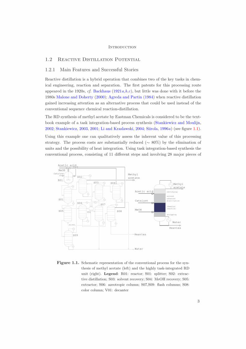
The RD synthesis of methyl acetate by Eastman Chemicals is considered to be the text-book example of a task integration-based process synthesis (Stankiewicz and Moulijn,2002; Stankiewicz, 2003, 2001; Li and Kraslawski, 2004; Siirola, 1996a) (see figure 1.1).
Using this example one can qualitatively assess the inherent value of this processingstrategy. The process costs are substantially reduced (∼ 80%) by the elimination ofunits and the possibility of heat integration. Using task integration-based synthesis theconventional process, consisting of 11 different steps and involving 28 major pieces of
Acetic acid
Catalyst
MeOH
rectifying
solvent
enhanceddistillation
chemicalreaction
stripping
Methylacetate
Water
Heavies
S08
Acetic acid
MeOHCatalyst
Heavies
Water
Methylacetate
Solvent
S04S03
S02
S01
R01
S06
S05
S09
S07
V01
Figure 1.1. Schematic representation of the conventional process for the syn-
thesis of methyl acetate (left) and the highly task-integrated RD
unit (right). Legend: R01: reactor; S01: splitter; S02: extrac-
tive distillation; S03: solvent recovery; S04: MeOH recovery; S05:
extractor; S06: azeotropic column; S07,S09: flash columns; S08:
color column; V01: decanter
3

Chapter 1
equipment, is effectively replaced by a highly task-integrated RD unit.
The last decades have seen a significant increase in the number of experimentally re-search studies dealing with RD applications. For example, Doherty and Malone (2001)(see table 10.5) state more than 60 RD systems have been studied, with the synthesis ofmethyl t -butyl ether (MTBE) and ethyl t -butyl ether (ETBE) gaining considerable at-tention. Taking an industrial perspective Stankiewicz (2003) lists the following processesas potential candidates for RD technology: (i) decomposition of ethers to high purityolefins; (ii) dimerization; (iii) alkylation of aromatics and aliphatics (e.g. ethylbenzenefrom ethylene and benzene, cumene from propylene and benzene); (iv) hydroisomeriza-tions; (v) hydrolyses; (vi) dehydrations of ethers to alcohols; (vii) oxidative dehydro-genations; (viii) carbonylations (e.g. n-butanol from propylene and syngas); and (ix )C1 chemistry reactions (e.g. methylal from formaldehyde and methanol). Recently, inthe frame of fine chemicals technology Omota et al. (2001, 2003) propose an innovativeRD process for the esterification reaction of fatty acids. The feasibility of this process isfirstly suggested using a smart combination of thermodynamic analysis and computersimulation (Omota et al., 2003). Secondly, the proposed design methodology is suc-cessfully applied to a representative esterification reaction in the kinetic regime (Omotaet al., 2001).
Process development, design and operation of RD processes are highly complex tasks.The potential benefits of this intensified process come with significant complexity inprocess development and design. The nonlinear coupling of reactions, transport phe-nomena and phase equilibria can give rise to highly system-dependent features, possiblyleading to the presence of reactive azeotropes and/or the occurrence of steady-state mul-tiplicities (cf. section §2.9). Furthermore, the number of design decision variables forsuch an integrated unit is much higher than the overall design degrees of freedom ofseparate reaction and separation units. As industrial relevance requires that designissues are not separated from the context of process development and plant operations,a life-span perspective was adopted for the research presented in this thesis.
1.2.2 Technical Challenges in the Process Design and Operation of Reac-
tive Distillation
A generalized applicability of RD technology is a key challenge for the process-orientedcommunity. Operational applicability is seen as strategic goal coupled with the de-velopment of (conceptual) design methodologies that can be used to support the RDdecision making process. Thus, the process systems engineering community is expectedto provide tools and supporting methods that can be used to faster develop and betteroperation of RD processes. Designing chemical process involves the joint considerationof process unit development and design programs (cf. section §4.5) and these are key
4
Introduction
challenges in RD process design.
A topic that is emerging as a challenge in the RD arena, is that, due to its system-dependency, RD processing is strongly limited by its reduced operation window (P,T ).This feasibility domain, which is determined by the overlapping area between feasiblereaction and distillation conditions (Schembecker and Tlatlik, 2003), spans a smallregion of the P-T space. On top of these two an additional window could be imposedby the equipment and material feasibility. In this context and within the developmentprogram, the key challenges for the RD community include: (i) the introduction of noveland more selective catalysts; (ii) the design of more effective and functional packingstructures (e.g. super X-pack (Stankiewicz, 2003)); and (iii) finding new applications.The first two challenges are strongly driven by the need to expand the RD operationalwindow beyond the current bounds for a given application.
1.3 Significance of Conceptual Design in Process Systems
Engineering
1.3.1 Scientific Setting of Conceptual Design in Process Systems Engi-
neering
Since its introduction, process systems engineering (PSE) has been used effectively bychemical engineers to assist the development of chemical engineering. In tying science toengineering PSE provides engineers with the systematic design and operation methods,tools that they require to successfully face the challenges of today’s chemical-orientedindustry (Grossman and Westerberg, 2000).
At the highest level of aggregation and regardless of length scale (i.e. from micro-scaleto industrial-scale) the field of PSE discipline relies strongly on engineers being ableto identify production systems. For the particular case of chemical engineering, a pro-duction system is defined as a purposeful sequence of physical, chemical and biologicaltransformations used to implement a certain function (Marquardt, 2004). A produc-tion system is characterized by its function, deliberate delimitation of its boundarieswithin the environment, its internal network structure and its physical behavior andperformance. These production systems are used to transform raw materials into prod-uct materials characterized by different chemical identities, compositions, morphologiesand shapes. From a PSE perspective the most remarkable feature of a system is itsability to be decomposed or aggregated in a goal-oriented manner to generate smalleror larger systems (Frass, 2005). Evidently, the level of scrutiny is very much linked tothe trade-off between complexity and transparency.
At a lower level of aggregation a system comprises the above mentioned sequence oftransformations or processes. Thus, a process can be regarded as a realization of a
5

Chapter 1
system and is made up of an interacting set of physical, chemical or biological trans-formations, that are used to bring about changes in the states of matter. These statescan be chemical and biological composition, thermodynamic phases, a morphologicalstructure and electrical and magnetic properties.
Going one level down in the aggregation scale gives us the chemical plant. This is nomore than the physical chemical process system. It is a man-made system, a chemicalplant, in which processes are conducted and controlled to produce valuable productsin a sustainable and profitable way. The conceptual process design (CPD) is made atthe following level of reduced aggregation. In the remainder of this section particularattention is given to CPD in the context of PSE.
Since its introduction, CPD has been defined in a wide variety of ways. CPD and PSEactivities are rooted in the concept of unit operations and the various definitions of CPDare basically process unit-inspired. The definition of CPD given by Douglas (1988) isregarded as the one which extracts the essence of this activity. Thus, CPD is definedas the task of finding the best process flowsheet, in terms of selecting the process unitsand interconnections among these units and estimating the optimum design conditions(Goel, 2004). The best process is regarded as the one that allows for an economical,safe and environmental responsible conversion of specific feed stream(s) into specificproduct(s).
Although this CDP definition might suggest a straight-forward and viable activity, theart of process design is complicated by the nontrivial tasks of (Grievink, 2003): (i)identifying and sequencing the physical and chemical tasks; (ii) selecting feasible typesof unit operations to perform these tasks; (iii) finding ranges of operating conditionsper unit operation; (iv) establishing connectivity between units with respect to massand energy streams; (v) selecting suitable equipment options and dimensioning; and(vi) control of process operations.
Moreover, the design activity increases in complexity due to the combinatorial explosionof options. This combination of many degrees of freedom and the constraints of thedesign space has its origin in one or more of the following: (i) there are many ways toselect implementations of physical/chemical/biological/information processing tasks inunit operations/controllers; (ii) there are many topological options available to connectthe unit operations (i.e. flowsheet structure), but every logically conceivable connectionis physically feasible; (iii) there is the freedom to pick the operating conditions overa physical range, while still remaining within the domain in which the tasks can beeffectively carried out; (iv) there is a range of conceivable operational policies; and (v)there is a range of geometric equipment design parameters. The number of possiblecombinations can easily run into many thousands.
The CPD task is carried out by specifying the state of the feeds and the targets on
6

Introduction
the output streams of a system (Doherty and Buzad, 1992; Buzad and Doherty, 1995)and by making complex and emerging decisions. In spite of its inherent complexity,the development of novel CPD trends has lately gained increasing interest from withinacademia and industry. This phenomenon is reflected in the number of scientific pub-lications focusing on CPD research issues and its applicability in industrial practice(Li and Kraslawski, 2004). For instance, the effective application of CPD practicesin industry has lead to large cost savings, up to 60% as reported by Harmsen et al.(2000) and the development of intensified and multifunctional units (e.g. the well-documented methyl acetate reactive distillation unit as mentioned by Stankiewicz andMoulijn (2002); Harmsen and Chewter (1999); Stankiewicz (2003)).
CPD plays an important role under the umbrella of process development and engineer-ing. As stated by Moulijn et al. (2001), process development features a continuousinteraction between experimental and design programs, together with carefully moni-tored cost and planning studies. The conventional course of process development in-volves several sequential stages: an exploratory stage, a conceptual process design, apreliminary plant flowsheet, miniplant(s) trials, trials at a pilot plant level and designof the production plant on an industrial scale. CPD is used to provide the first andmost influential decision-making scenario and it is at this stage that approximately 80%of the combined capital and operational costs of the final production plant are fixed(Meeuse, 2003). Performing individual economic evaluations for all design alternativesis commonly hindered by the large number of possible designs. Therefore, systematicmethods, based on process knowledge, expertise and creativity, are required to deter-mine which will be the best design given a pool of thousands of alternatives.
1.3.2 Developments in New Processes and Retrofits
From its introduction the development of CPD trends has been responding to the har-monic satisfaction of specific requirements. In the early stages of CPD developmenteconomic considerations were the most predominant issue to be taken into account.Seventy years on, the issues surrounding CPD methodologies have been extended toencompass a wide range of issues involving economics, sustainability and process re-sponsiveness (Almeida-Rivera et al., 2004b; Harmsen et al., 2000). Spatial and temporalaspects must be taken into account when designing a process plant. Additionally, thetime dimension and loss prevention are of paramount importance if the performanceof a chemical plant is to be optimized over its manufacturing life-span. This broadperspective accounts for the use of multiple resources (e.g. capital, raw materials andlabor) during the design phase and the manufacturing stages. In this context and inview of the need to support the sustainability of the biosphere and human society, thedesign of sustainable, environmentally benign and highly efficient processes becomes a
7

Chapter 1
major challenge for the PSE community. Identifying and monitoring potential losses ina process, together with their causes are key tasks to be embraced by a CPD approach.Means need to be put in place to minimize losses of mass, energy, run time availabilityand, subsequently, profit. Poor process controllability and lack of plant responsivenessto market demands are just two issues that need to be considered by CPD engineers ascauses of profit loss.
Li and Kraslawski (2004) have recently presented a detailed overview on the develop-ments in CPD, in which they show that the levels of aggregation in CPD (i.e. micro-,meso- and macroscales) have gradually been added to the application domain of CPDmethodologies. This refocus on the design problem has lead to a wide variety of suc-cess stories at all three scale levels and a coming to scientific maturity of the currentmethodologies.
At the mesolevel the research interests have tended towards the synthesis of heatexchange networks, reaction path kinetics and sequencing of multicomponent separa-tion trains (Li and Kraslawski, 2004). A harmonic compromise between economics,environmental and societal issues is the driving force at the CPD macrolevel. Underthe framework of multiobjective optimization (Clark and Westerberg, 1983), severalapproaches have been derived to balance better the trade-off between profitability andenvironmental concerns (Almeida-Rivera et al., 2004b; Kim and Smith, 2004; Lim et al.,1999). Complementary to this activity, an extensive list of environmental indicators(e.g. environmental performance indicators) has been produced in the last decades(Lim et al., 1999; Kim and Smith, 2004; Li and Kraslawski, 2004). At the CPD mi-crolevel the motivating force has been the demand for more efficient processes withrespect to equipment volume, energy consumption and waste formation (Stankiewiczand Moulijn, 2002). In this context a breakthrough strategy has emerged: abstractionfrom the historically equipment-inspired design paradigm to a task-oriented processsynthesis. This refocus allows for the possibility of task integration and the designof novel unit operations or microsystems, which integrate several functions/tasks andreduce the cost and complexity of process systems (Grossman and Westerberg, 2000).An intensified unit is normally characterized by drastic improvements, sometimes inan order of magnitude, in production cost, process safety, controllability, time to themarket and societal acceptance (Stankiewicz, 2003; Stankiewicz and Moulijn, 2002).Among the proven intensified processes reactive distillation (RD) occupies a place ofpreference and it is this which is covered in the course of this thesis, coupled with anemphasis on RD conceptual design.
8

Introduction
1.3.3 Key Challenges in the Design of Reactive Distillation
Due to its highly complex nature, the RD design task is still a challenge for the PSEcommunity. The following intellectually challenging problems need to be considered bythe PSE community (Grossman and Westerberg, 2000): (i) design methodologies forsustainable and environmentally benign processes; (ii) design methodologies for inten-sified processes; (iii) tighter integration between design and the control of processes;(iv) synthesizing plantwide control systems; (v) optimal planning and scheduling fornew product discovery; (vi) planning of process networks; (vii) flexible modeling envi-ronments; (viii) life-cycle modeling; (ix ) advanced large-scale solving methods; and (x )availability of industrial nonsensitive data. An additional PSE specific challenge is todefine a widely accepted set of effectiveness criteria that can be used to assess processperformance. These criteria should take into account the economic, sustainability andresponsiveness/controllability performances of the design alternatives.
1.4 Scope of Research
During the course of this PhD thesis we deal with the design of grassroots reactivedistillation processes. At this high level of aggregation, the process design is far morecomprehensive than for most of the industrial activities (e.g. retrofit, debottleneckingand optimal operation of existing equipment) as it involves a wide range of domainknowledge and augmented (design) degrees of freedom.
Here it becomes necessary to introduce an explanatory caveat regarding the conceptof life span. From a formal standpoint this term includes all stages through whicha production system or activity passes during its lifetime (Schneider and Marquardt,2002). From a product perspective, for instance, the life span describes one, the life ofthe product from cradle to grave (Meeuse, 2003; Korevaar, 2004). Two, each processstep along the cradle-to-grave path is characterized by an inventory of the energy, ma-terials used and wastes released to the environment and an assessment of the potentialenvironmental impact of those emissions (Jimenez-Gonzalez et al., 2000, 2004). If ourviewpoint is the process rather than the product life span, we can foresee a sequenceof stages including need identification, research and development, process design, plantoperation and retrofit/demolition. As covering all these process stages in a uniquemethodology is a highly demanding task, we limited our research to the sustainabilityaspects that are exclusively under the control of the design and operational phases.Thus, in our scope of life span we do not consider any sustainability issue related tofeed-stock selection, for example, (re-)use of catalyst, (re-)use of solvent, among others.
A life-span inspired design methodology (LiSp-IDM) is suggested as the first attempttowards a design program strategy. Although more refined and detailed approaches
9

Chapter 1
are expected to be introduced in the future, their underlying framework will probablyremain unchanged. In this framework, a life-span perspective is adopted, accounting forthe responsible use of multiple resources in the design and manufacturing stages and asystems’ ability to maintain product specifications (e.g. compositions and conversion) ina desired range when disturbances occur. In this thesis and for the first time, economic,sustainability and responsiveness/controllability aspects are embedded within a singledesign approach. The driving force behind this perspective is derived from regardingthe design activity as a highly aggregated and large-scale task, in which process unitdevelopment and design are jointly contemplated.
All the aforementioned features of the LiSp-IDM are captured in the following definition,
LiSp-IDM is taken to be a systematic approach that can be used to solvedesign problems from a life-span perspective. In this context, LiSp-IDM issupported by defining performance criteria that can be used to account forthe economic performance, sustainability and responsiveness of the process.Moreover, LiSp-IDM framework allows a designer to combine, in a sys-tematic way, the capabilities and complementary strengths of the availablegraphical and optimization-based design methodologies. Additionally, thisdesign methodology addresses the steady-state behavior of the conceivedunit and a strong emphasis is given to the unit dynamics.
The following set of goal-oriented engineering questions were formulated based in theabove definition,
• Question 1. What benefits can be gained from having a more integrated designmethodology?
• Question 2. What are the practical constraints that need to be considered froma resources point of view (i.e. time, costs, tools and skill levels), when developingand applying a design methodology in a work process?
• Question 3. What are the essential ingredients for such a design methodology?
Additionally, a set of specific scientific design questions were formulated based on thesteps of a generic design cycle,
• Question 4. What is the domain knowledge required and which new buildingblocks are needed for process synthesis?
• Question 5. What are the (performance) criteria that need to be considered froma life-span perspective when specifying a reactive distillation design problem?
10
Introduction
• Question 6. What (new) methods and tools are needed for reactive distillationprocess synthesis, analysis and evaluation?
• Question 7. Are there structural differences and significant improvements indesigns derived using conventional methodologies from those obtained using anintegrated design methodology?
These questions will be either qualitatively or quantitatively answered during the courseof this thesis.
1.5 Outline and Scientific Novelty of the Thesis
This dissertation is divided into several chapters, covering the conceptual design of grass-roots RD processes. The fundamentals, weaknesses and opportunities of RD processingare addressed in chapter 2. A detailed description of the current design methodologies inRD forms the subject of chapter 3. Special attention is paid to the identification of themethodologies’ strengths and missing opportunities and a combination of methodologycapabilities is used to derive a new multiechelon† design approach, which is presented indetail in chapter 4. The essential elements of this design approach are then addressedusing the synthesis of methyl-tert butyl ether as tutorial example. Chapter 5 deals withthe feasibility analysis of RD processing based on an improved residue curve mappingtechnique and column sequencing. In chapter 6, the focus is on the synthesis of inter-nal spatial structures, in particular. A multilevel modeling approach and the dynamicoptimization of spatial and control structures in RD are introduced. The steady-stateand dynamic performance in RD form the subjects of chapter 7. The performance cri-teria embedded in the proposed RD methodology are covered in chapter 8, in which alife-span perspective is adopted leading to the definition of performance criteria relatedto economics, thermodynamic efficiency and responsiveness. The interactions betweenthose performance criteria in the design of RD are explored in particular. The infor-mation generated in the previous chapters is summarized in chapter 9, where a finalevaluation of the integrated design is presented. The chapter is concluded with remarksand recommendations for further research in the RD field.
The scientific novelty of this work is embedded in several areas.
Formulation of an extended design problem. A renewed and more comprehensivedesign problem in RD is formulated in the wider context of process development andengineering. The nature of the extension is found in the identification of the design
†The term echelon refers to one stage, among several under common control, in the
flow of materials and information, at which items are recorded and/or stored (source:
http://www.pnl.com.au/glossary/cid/32/t/glossary visited in August 2005).
11
Chapter 1
decision variables and their grouping into three categories: (i) those related to physicaland operational considerations; (ii) those related to spatial issues; and (iii) those relatedto temporal considerations.
Integrated design methodology. An integrated design is presented (i.e. LiSp-
IDM) based on a detailed analysis of the current design methodologies in RD. Asindustrial relevance requires that design issues are not separated from the context ofprocess development and plant operations, a life-span perspective was adopted. Theframework of this methodology was structured using the multiechelon approach, whichcombines in a systematic way the capabilities and complementary strengths of theavailable graphical and optimization-based design methodologies. This approach issupported by a decomposition in a hierarchy of imbedded design spaces of increasingrefinement. As a design progresses the level of design resolution can be increased, whileconstraints on the physical feasibility of structures and operating conditions derivedfrom first principles analysis can be propagated to limit the searches in the expandeddesign space.
Improvement in design tools. The proposed design methodology is supportedby improved design tools. Firstly, the residue curve mapping technique is extendedto the RD case and systematically applied to reactive mixtures outside conventionalcomposition ranges. This technique is found to be particularly useful for the sequencingof (non-) reactive separation trains. Secondly, the models of the process synthesisbuilding blocks are refined leading to the following sub-improvements: (i) a refinedmodular representation of the building blocks; (ii) changes/improvements in the modelsof the building blocks; and (iii) enhancements in synthesis/analysis tools. Regardingthe last item, a multilevel modeling approach is introduced with the aim of facilitatingthe decision-making task in the design of RD spatial structures.
Performance criteria. To account for the process performance from a life-spanperspective, criteria related to economic, sustainability and responsiveness aspects aredefined and embraced in the proposed design methodology. For the first time the inter-actions between economic performance, thermodynamic efficiency and responsivenessin RD process design are explored and possible trade-offs are identified. This researchsuggests that incorporating a sustainability-related objective in the design problem for-mulation might lead to promising benefits from a life-span perspective. On one hand,exergy losses are accounted for, aiming at their minimization and on the other handthe process responsiveness is positively enhanced.
12

“The important thing is not to stop questioning. Curiosity
has its own reason for existing.”
Albert Einstein, scientist and Nobel prize laureate
(1879-1955)
2Fundamentals of Reactive Distillation
The combination of reaction and separation processes in a single unit has been found
to generate several advantages from an economic perspective. However, from a design
and operational point of view this hybrid process is far more complex than the indi-
vidual and conventional chemical reaction - distillation operation. In this chapter a
general description of the fundamentals of reactive distillation is presented. A sound
understanding and awareness of these issues will enable more intuitive explanations
of some of the particular phenomena featured by a RD unit. The starting point of our
approach is the systematic description of the physical and chemical phenomena that
occur in a RD unit. Relevant combinations of those phenomena are grouped in levels
of different aggregation scrutiny (i.e. one-stage, multistage, distributed and flowsheet
levels). Each level deals with the particularities of the involved phenomena. More-
over, each level is wrapped-up with the identification of the design decision variables
that are available to influence or control the phenomena under consideration.
13

Chapter 2
2.1 Introduction
It is a well-known and accepted fact that complicated interactions between chemicalreaction and separation make difficult the design and control of RD columns. Theseinteractions originate primarily from VLL equilibria, VL mass transfer, intra-catalystdiffusion and chemical kinetics. Moreover, they are considered to have a large influenceon the design parameters of the unit (e.g. size and location of (non)-reactive sections,reflux ratio, feed location and throughput) and to lead to multiple steady states (Chenet al., 2002; Jacobs and Krishna, 1993; Guttinger and Morari, 1999b,a), complex dy-namics (Baur et al., 2000; Taylor and Krishna, 2000) and reactive azeotropy (Dohertyand Malone, 2001; Malone and Doherty, 2000).
To provide a clear insight on the physical and chemical phenomena that take placewithin a RD unit, a systems approach is proposed according to the following classifica-tion features,
• spatial scrutiny scale: where the system can be lumped with one-stage, lumpedwith multistages or distributed. Note that the spatial scales involved in thisresearch are approached from bottom to top. A schematic representation of thesescales is given in figure 2.1,
• contact with the surroundings: where the system can be either open or closed,
• equilibrium between the involved phases: where they can be either in equilibriumor non-equilibrium, and
• transient response: where the non-equilibrium system can be regarded as station-ary or dynamic.
x y
y
xI
I
N V
liquid phase gas phase
film
inte
rpha
se
NL
z
Spatial scale
Q
F feed,Vn
Rx
F Vn+1
F side,Vn
F Vn
F feed,Ln
F Ln
F Ln-1
F side,Ln
1
15
9
10
MeOH
C4-stream
3
MTBE(>99%m)
MTBE(<0.1%m)
reactivezone
P
L
L
T
Fcool
Pcond
lcond
lreb
Treb
Qreb
Fout,Lcond
Fout,Lreb
FR,L FD,L
B1
to sequence zone b
M1F
D2
D1
B2MeOH
C1 C2
µm m Km
Figure 2.1. Schematic representation of the relevant spatial scales in reactive
distillation
These four features can be smartly combined leading to 10 different system instances,as listed in table 2.1. Instances 2, 5 and 8 are not further considered in this explanatorychapter because of their reduced practical interest. As there is no interaction between
14

Fundamentals of Reactive Distillation
the system and surroundings, the closed system will gradually reach equilibrium statedue to dynamic relaxation. Furthermore, instances 4, 7 and 10 are closely linked totheir associated steady-state situation and are then embedded within instances 3, 6 and9, respectively.
This analysis results in instances 1 (lumped one-stage, closed and equilibrium), 3(lumped one-stage, open and non-equilibrium), 6 (lumped multistage, open and non-equilibrium) and 10 (distributed, open and non-equilibrium) for further considerationin the course of this chapter. A first classification of these instances is performed basedon their spatial structure, aiming to cover the whole range of physical and chemicalphenomena that occur in a RD unit. The following levels are then defined,
Level A. One-stage level: where the system is represented by a single lumped stage[embracing instances I1 and I3],
Level B. Multi-stage level: where the system is represented by a set of interconnectedtrays [embracing instance I6], and
Level C. Distributed level: where the system is defined in terms of an spatial coor-dinate [embracing instance I10].
Recalling the engineering and scientific design questions given in chapter 1, in thischapter we address question 4, namely,
• What is the domain knowledge required and which new building blocks are neededfor process synthesis?
As the nature of this chapter is explanatory, the knowledge presented is borrowed fromvarious scientific sources. Thus, the novelty of this chapter is exclusively given by thesystems approach adopted to address the phenomena description. Note that the spatialscales involved in this research are approached from bottom to top.
Table 2.1. Systems instances to be considered for the analysis of physical and
chemical processes in a RD unit
Instance Spatial level Contact Phase behavior Time response
I1 lumped one-stage closed equilibrium
I2 lumped one-stage closed non-equilibrium dynamic relaxation
I3/I4 lumped one-stage open non-equilibrium steady state/dynamic
I5 lumped multistage closed non-equilibrium dynamic relaxation
I6/I7 lumped multistage open non-equilibrium steady state/dynamic
I8 distributed closed non-equilibrium dynamic relaxation
I9/I10 distributed open non-equilibrium steady state/dynamic
15

Chapter 2
2.2 One-stage Level: Physical and Chemical (non-) Equilib-
rium
Phase equilibrium. For a nc-component mixture phase equilibrium is determinedwhen the Gibbs free energy G for the overall open system is at a minimum (Biegleret al., 1997),
Function : minn
(j)i ,µ
(j)i
n× G =i=nc∑i=1
j=np∑j=1
n(j)i × µ
(j)i
s.t. :j=np∑j=1
n(j)i = ni,0 +
k=nrx∑k=1
νi,k × εk, i ∈ Znc (2.1)
n(j)i ≥ 0,
where ni is the total number of moles for component i, n(α)i is the number of moles of
component i in phase (α), n is the total number of moles, np is the number of phasesin the system, nrx is the number of chemical reactions, εk is the extent of reaction k
and µ(α)i is the chemical potential of component i in phase (α) and given by,
µ(α)i = G0
i + R× T × ln f (α)i , i ∈ Z
nc . (2.2)
In the previous expression, the fugacity of component i in phase (α), f (α)i , is estimated
in terms of the fugacity coefficient and component’s concentration in phase (α) (i.e.ai = γi × xi).
The necessary condition for an extremum of the minimization problem is given by theequality of chemical potentials across phases and the thermal and mechanical equilib-rium,
µ(j)i = µ
(k)i , j, k ∈ Znp , (2.3)
T (j) = T (k), j, k ∈ Znp , (2.4)
P (j) = P (k), j, k ∈ Znp . (2.5)
For the particular case of vapor-liquid equilibrium, the necessary conditions results inthe well-known expression,
yi × Φi × P = xi × γi × p0i , i ∈ Z
nc . (2.6)
A detailed description of the thermodynamic model used to derive the VL equilibriumexpression 2.6 is presented in appendix B.
16

Fundamentals of Reactive Distillation
Chemical Equilibrium. For a single-phase fluid and open system a fundamentalthermodynamic property relation is given by Smith and van Ness (1987),
d(n× G) = (n× V )dP − (n× S)dT +i=1∑
j=nc
µi × dni, (2.7)
where dni = νi × dε denotes the change in mole numbers of component i, νi is thestoichiometric coefficient of component i, ε is the extent of reaction and S is the molarentropy of the system.
Knowing that n×G is a state function, an expression is obtained for the rate of changeof the total Gibbs energy of the system with the extent of reaction at constant T andP,
i=1∑j=nc
νi × µi =[∂(n× G)
∂ε
]T,P
. (2.8)
At equilibrium conditions the Gibbs energy expression 2.8 equals to zero and allowsone to define the equilibrium state in terms of the measurable temperature-dependentequilibrium constant Keq,
−R× T × lnKeq =i=nc∑i=1
νi × G0i , (2.9)
Keq =i=nc∏i=1
aνi
i , (2.10)
where R is the universal gas constant, ai denotes the activity of specie i and theexponent zero represents the standard state. Note that the liquid-phase activity ai andfugacity are related according to the expression (Malanowski and Anderko, 1992),
fLi = f0
i × ai, (2.11)
where f0i is the reference state fugacity, which is estimated for pure liquid at equilibrium
conditions.
2.3 Multi-stage Level: Combined Effect of Phase and Chem-
ical Equilibrium
For the sake of clarifying the interaction between chemical and phase equilibrium in RD,several concepts need to be introduced. Note, firstly, that the spatial configuration atthis level is assumed to allow efficient contact between the phases and in an staged-wiseoperation.
The concept of stoichiometric lines captures the concentration change of a given speciedue to chemical reaction (Frey and Stichlmair, 1999b).
17

Chapter 2
Let ni0 be the number of moles of specie i at time t0 in a closed system. Chemicalreactions proceed according to their extent of reaction εj (j ∈ Znrx). After chemicalequilibrium is reached, the number of moles at anytime is is given by,
ni = ni0 +∑
j
νi,j × εj , i ∈ Znc , j ∈ Z
nrx . (2.12)
Knowing that the total number of moles in the closed system equals to,
n = n0 +∑
j
νtotal,j × εj , j ∈ Znrx , (2.13)
it follows that the stoichiometric line is expresses as,
xi =xi0(νk − νtotal × xk) + νi(xk − xk0 )
νk − νtotal × xk0
, i ∈ Znc , (2.14)
where νtotal is the sum of the stoichiometric coefficients (νtotal =∑νi) and k is a
reference component (k ∈ Znc).
Any mixture apart from the chemical reaction equilibrium reacts along these lines tothe corresponding equilibrium state (Frey and Stichlmair, 1999a). Thus, a family ofstoichiometric lines results from the variation of initial components concentration, whichintercept at the pole π (figure 2.2), whose concentration is defined as xiπ = νi × ν−1
total.
Another term to be introduced is the widespread distillation line concept, commonlyused to depict phase equilibrium in conventional distillation. According to Frey andStichlmair (1999b) and Westerberg et al. (2000), distillation lines correspond to theliquid concentration profile within a column operating at total reflux. It follows from thisdefinition that a distillation line is characterized by sequential steps of phase equilibriaand condensation. Thus, the following sequence is adopted for the case of an equilibriumstage model,
xi1phase equilibrium−−−−−−−−−−−→ y∗i1
condensation−−−−−−−−→ x∗i1 · ·· (2.15)
The starting point of this sequence is the reactive mixture x1 (depicted conventionally onthe chemical equilibrium line in figure 2.2). This liquid mixture is in phase equilibriumwith the vapor y∗1 , which is totally condensed to x∗1.
It is relevant to mention that an alternative concept might be used to depict the phaseequilibrium: residue curve (Fien and Liu, 1994; Westerberg and Wahnschafft, 1996). Incontrast to distillation lines, residue curves track the liquid composition in a distillationunit operated at finite reflux. Although for finite columns distillation and residue linesdiffer slightly, this difference is normally not significant at the first stages of design.Graphically, the tangent of a residue curve at liquid composition x intercepts the dis-tillation line at the vapor composition y in phase equilibrium with x (Fien and Liu,1994). A more detailed application of residue curve is covered in chapter 5.
18

Fundamentals of Reactive Distillation
A
B
reactiveazeotrope
1*
1
2
3
3*
2*
A
1011
12 13
12*11*
10*A*
Stoichiometriclines
C
Figure 2.2. Representation of stoichiometric and reactive distillation lines for
the reactive system A-B-C undergoing the reaction A+B � C.
Remark: π denotes the pole at which stoichiometric lines co-
incide, xiπ = νi/Σνj . Legend: dashed line: stoichiometric
line; dotted line: phase-equilibrium line; continuous line: chem-
ical equilibrium line. System feature: T boilC > T boil
B > T boilA .
(adapted from Frey and Stichlmair (1999b)).
A third concept is introduced when chemical reaction and phase equilibrium phenomenaare superimposed in the unit: reactive distillation lines. The following sequence of phaseequilibrium→chemical reaction steps is adopted for the evolution of reactive distillationlines,
xi1phase eq.−−−−−−→ y∗i1
condensation−−−−−−−−→ x∗i1reaction−−−−−→ xi2
phase eq.−−−−−−→ y∗i2condensation−−−−−−−−→ x∗i2 · ·· (2.16)
The starting point of this sequence is the reactive mixture x1 on the chemical equilibriumline. This liquid mixture is in phase equilibrium with the vapor y∗1 , which is totallycondensed to x∗1. Since this mixture is apart from the chemical equilibrium line, itreacts along the stoichiometric line to the equilibrium composition x2. As can be seenin figure 2.2, the difference of the slope between the stoichiometric and liquid-vaporequilibrium lines defines the orientation of the reactive distillation lines. This differencein behavior allows one to identify a point, at which both the phase equilibrium andstoichiometric lines are collinear and where liquid concentration remains unchanged.This special point (labelled ‘A’ in figure 2.2) is conventionally referred to as reactiveazeotrope and is surveyed in section §2.4.
19

Chapter 2
2.4 Multi-stage Level: Reactive Azeotropy
Unlike its nonreactive counterpart, reactive azeotropes occur in both ideal and nonidealmixtures, limiting the products of a reactive distillation process in the same way thatordinary azeotropy does in a nonreactive distillation operation (Doherty and Buzad,1992; Harding and Floudas, 2001). In both cases, however, the prediction whether agiven mixture will form (reactive) azeotropes and the calculation of their compositionsare considered essential steps in the process design task (Harding et al., 1997). Due tothe high non-linearity of the thermodynamic models this prediction is not trivial at alland requires an accurate and detailed knowledge of the phase equilibria (expressed byresidue or distillation lines), accurate reaction equilibria and the development of special-ized computational methods. In addition to the difficulty of enclosing all azeotropes in amulticomponent mixture, azeotropy is closely linked to numerous phenomena occurringin the process (e.g. run-away of nonreactive azeotropes and the vanishing of distillationboundaries) as mentioned by Barbosa and Doherty (1988a); Song et al. (1997); Freyand Stichlmair (1999b); Harding and Floudas (2000); Maier et al. (2000); Harding andFloudas (2001). Accordingly, a solid understanding of the thermodynamic behavior ofazeotropes becomes a relevant issue to address in process development. It allows one todetermine whether a process is favorable and to account for the influence of operatingconditions on process feasibility.
From a physical point of view, the necessary and sufficient condition for reactive azeotropyis that the change in concentration due to distillation is totally compensated for by thechange in concentration due to reaction (Frey and Stichlmair, 1999a,b). As mentionedin the previous section, this condition is materialized when a stoichiometric line is co-linear with the phase equilibrium line, as depicted in figure 2.2. If the residue curvesare used to represent the phase equilibrium, the reactive azeotropic compositions areto be found according to the following graphical procedure (figure 2.3): (i) the pointsof tangential contact between the residue and stoichiometric lines (marker: •) define acurve of potential reactive azeotropes (thick line), which runs always between singularpoints; (ii) a reactive azeotrope (RAz, marker: ◦) then occurs at the intersection pointbetween the chemical equilibrium line and the curve of potential reactive azeotropes.
Based on the graphical estimation of reactive azeotropes, Frey and Stichlmair (1999a)establishes the following rules of thumb,
� Rule 1. A maximum reactive azeotrope occurs when the line of possible reactiveazeotropes runs between a local temperature maximum and a saddle point and whenthere is only one point of intersection with the line of chemical equilibrium,
� Rule 2. A minimum reactive azeotrope occurs when the line of possible reactiveazeotropes runs between a local temperature minimum and a saddle point and whenthere is only one point of intersection with the line of chemical equilibrium.
20

Fundamentals of Reactive Distillation
A
B
Stoichiometriclines
C
Residuelines
Loci of reactiveazeotropes
RAz
K
Figure 2.3. Graphical determination of reactive azeotropy. Symbols: (◦):reactive azeotrope RAz at the given chemical equilibrium constant
Keq; π: pole at which stoichiometric lines coincide, xiπ = νi/Σνj .
System features: chemical reaction A+B � C. (adapted from
Frey and Stichlmair (1999b)).
A practical limitation of this method is imposed by its graphical nature. Thus, thismethod has been only applied to systems of three components at the most undergoinga single reaction. Extending this method to systems with nc > 3 might not be feasibledue to the physical limitation of plotting the full-component composition space.
From a different and more rigorous perspective, a reactive azeotrope might be char-acterized by the satisfaction of the following necessary and sufficient conditions for asystem undergoing a single equilibrium chemical reaction (Barbosa and Doherty, 1987b;Doherty and Buzad, 1992),
y1 − x1
ν1 − νtotal × x1=
yi − xi
νi − νtotal × xi, i ∈ [2, nc − 1]. (2.17)
It is relevant to point out that the azeotropy expression 2.17 also applies to the lastcomponent (nc) as may be verified by knowing that
∑i=nc
i=1 xi =∑i=nc
i=1 yi = 1 (Barbosaand Doherty, 1987b).
These necessary and sufficient conditions for reactive azeotropes have been generalizedand theoretically established for the case of multicomponent mixtures undergoing multi-ple equilibrium chemical reactions by Ung and Doherty (1995b). The starting point fortheir analysis is the introduction of transformed compositions . It is widely recognizedthat mole fractions are not the most convenient measures of composition for equilibriumreactive mixtures, as they might lead to distortions in the equilibrium surfaces (Barbosaand Doherty, 1988a; Doherty and Buzad, 1992). In order to visualize in a much more
21

Chapter 2
comprehensive manner the presence of reactive azeotropes, a transformed compositionvariable has been introduced by Doherty and co-workers (Barbosa and Doherty, 1987a;Doherty and Buzad, 1992; Ung and Doherty, 1995a,c; Okasinski and Doherty, 1997),
Xi ≡ νk × xi − νi × xk
νk − νtotal × xk, Yi ≡ νk × yi − νi × yk
νk − νtotal × yk, i ∈ Z
nc , i �= k, (2.18)
where k denotes a reference component that satisfies the following conditions for νtotal:(i) k is a reactant if νtotal > 0; (ii) k is a product if νtotal < 0, and (iii) k is a productor reactant if νtotal = 0.
The necessary and sufficient conditions for reactive azeotropy for the multicomponent,multireaction system can be then expressed in terms of the transformed variables (Ungand Doherty, 1995b),
Xi = Yi, i ∈ Znc−2. (2.19)
For this system, the transformed compositions are given by the following generalizedexpressions,
Xi =xi − νT
i (Vref)−1xref
1 − νTtotal(Vref)−1xref
, i ∈ Znc−nrx , (2.20)
Yi =yi − νT
i (Vref)−1yref
1 − νTtotal(Vref)−1yref
, i ∈ Znc−nrx , (2.21)
where
Vref =
ν(nc−nrx+1),1 · · · ν(nc−nrx+1),nrx
... νi,r
...νnc,1 · · · νnc,nrx
,
dτw = dt×(
1−νTtotal(Vref)
−1yref
1−νTtotal(Vref)−1xref
)× V/L,
(2.22)
where νTi is the row vector of stoichiometric coefficients for component i ∈ Znc−nrx
in all the nrx reactions [νi,1 νi,2 · · · νi,R], νTtotal is the row vector of the total mole
number change in each reaction[∑i=nc
i=1 νi,1 · · ·∑i=nc
i=1 νi,nrx
], ref denotes the reference
components for the nrx reactions, numbered from nc − nrx + 1 to nc and Vref is thesquare matrix of stoichiometric coefficients for the nrx reference components in the nrx
reactions.
These azeotropy expressions 2.19 state that in the space of transformed compositionvariables the bubble-point and dew-point surfaces are tangent at an azeotropic state(Barbosa and Doherty, 1988a), allowing the azeotropes to be found easily by visualinspection in the reactive phase diagram for the case of nc − nrx ≤ 3 (figure 2.4).For systems beyond this space, a graphical determination of azeotropes might not befeasible.
22

Fundamentals of Reactive Distillation
0.2 0.4 0.6 0.8 10
0.1
0.2
0.3
0.4
0.5
0.6
0.7
0.8
0.9
1
X methanol [−]
Y methanol [−]
Reactive azeotrope
Figure 2.4. Phase diagram for methanol in the synthesis of MTBE expressed
in terms of transformed compositions (equation 2.18). Remarks:
the location of the reactive azeotrope is tracked down at the inter-
section of the residue curve and the line X = Y ; reacting mixtures
of various compositions are depicted. System features: oper-
ating pressure is 11·105 Pa; inert nC4 is present in the mixture.
Note that the azeotropy expression 2.19 holds also for pure components and nonreactiveazeotropes surviving reaction. Moreover, the necessary and sufficient condition forreactive azeotropy resembles largely the conditions for nonreactive azeotropy in termsof molar fractions,
xi = yi, i ∈ Znc . (2.23)
2.5 Non-equilibrium Conditions and Rate Processes
Phase non-equilibrium. If a chemical potential gradient exists between two adjacentand homogenous phases, the system is not in local phase equilibrium and a rate-limitedmass transfer phenomenon occurs. A momentum balance of specie i results in thefollowing expression for the driving force exerted on i as a function on the friction
23

Chapter 2
forces due to diffusive motion of all other species,
fi =i=nc∑j �=i
ζi,j × xj × (udiffi − udiff
j ), i, j ∈ Znc , (2.24)
where f is the frictional force, udiffi is the diffusive velocity of specie i and ζi,j is the
friction coefficient between species i and j.
This expression is the well-known Maxwell-Stefan equation (MSE) and states that thedriving force on a specie i in a mixture equals the sum of the friction forces between i
and the other species j. MSE applied to multicomponent mixtures offers obviously adetailed description of the transfer phenomena, but on the other hand the model com-plexity and parametric uncertainty are considerably increased. The rate-based approachis of particular importance in (reactive) distillation, as the use of conventional stage effi-ciencies might be resulting in absurd variations (−∞ to +∞ as acknowledged by Keniget al. (2000); Wesselingh (1997)). If MSE 2.24 is expressed in terms of Maxwell-Stefandiffusivities D, species flux N, average concentration Ctotal and chemical potential µ,the following MSE is obtained in a multidimensional space (Wesselingh and Krishna,2000),
yi
R×T V ∇T,PµVi =
j=nc∑j=1;j �=i
yi×NVj −yj×N
Vi
CVtotal×DV
ij, i ∈ Znc ,
xi
R×T L ∇T,PµLi =
j=nc∑j=1;j �=i
xi×NLj −xj×N
Li
CLtotal×DL
ij, i ∈ Znc .
(2.25)
A fully description of the non-equilibrium mass transfer phenomenon embraces simulta-neously a Maxwell-Stefan diffusion model and a flow model. The most commonly usedapproach is the film model , which is addressed in more detail in the explanatory note2.1.
Rate-limited chemical reaction. According to the universally applicable law ofmass action, the rate of chemical reaction is directly proportional to the active massesof each of the reactants. For the particular case of a system not in chemical equilibrium,the term
∏i=nc
i=1 aνi
i is commonly called reaction quotient. At the limiting case, the non-equilibrium system tends to equilibrium state, which results in the reaction quotienttending to Keq. The degree of separation between current system state and chemicalequilibrium might be estimated by computing the Damkohler number,
Da =tprocess
treaction. (2.32)
According to this definition, Damkohler number gives the ratio of the characteristicprocess time to the characteristic reaction time (Doherty and Malone, 2001) and cap-tures effectively the major dependence of conversion, production rate and product pu-rities on the feed flowrate, catalyst level and holdup (Chen et al., 2002). For an open
24

Fundamentals of Reactive Distillation
Film model is undoubtedly the most widespread approach for the rate-based mass and heat transfer
through an interface (Wesselingh and Krishna, 2000). It effectively combines species diffusion
and fluid flows and is based on the assumption that the resistance to mass and heat transfer is
exclusively concentrated in a thin film where steady state diffusion and mass and heat convection
take place (figure 2.5).
Thus, the interfacial mass and heat transfer fluxes are composed of a laminar, steady state
diffusion term in the stagnant film and a convection term from the complete turbulent bulk
phase (Taylor and Krishna, 1993),
vapor NVi = JV
i + NVtotal × yi, i ∈ Znc ,
EV = hVHX · (T I − TV ) +
∑i=nci=1 NV
i × HVi .
liquid NLi = JL
i + NLtotal × xi, i ∈ Znc ,
EL = hLHX × (TL − T I) +
∑i=nci=1 NL
i × HLi ,
(2.26)
with
N(α)total =
i=nc∑i=1
N(α)i , (α) ∈ {liquid, vapor}, (2.27)
where J(α)i is the diffusion flux of component i in phase (α), H
(α)i is the partial molar enthalpy
of component i in phase (α) and hHX is the heat transfer coefficient.
With the assumption of perfectly mixed bulk phases and considering the flux direction (figure
2.5), the diffusion flux may be re-written in terms of the concentration gradient between the
bulk and the interface,
JVi = CV
total · kVi,m(yI
i − yi),
JLi = CL
total · kLi,m(xi − xI
i ), i ∈ Znc ,(2.28)
with
C(α)total =
∑C
(α)i , (2.29)
where k(α)i,m is the mass transfer coefficient of component i in the mixture m in phase (α).
The film model assumes additionally, no accumulation in the interface and equilibrium state at
the interface,
NLi = NV
i , i ∈ Znc ,
EL = EV ,(2.30)
and
yIi = fk(xI
i , T ), i ∈ Znc , (2.31)
where fk is a nonlinear function of the distribution coefficients.
Note 2.1. Rate-based mass and heat transfer: the film model
25

Chapter 2
x y
y
xI
I
N V
liquid phase gas phase
film
inte
rpha
se
NL
z
Figure 2.5. Schematic representation of the Film Model. The mass and heat
transfer fluxes are assumed to be positive in the direction liquid
→ vapor.
system, for instance, with phase holdup M , feed flowrate F and undergoing a chemicalreaction, the Damkohler number might be given as follows,
homogenously catalyzed Da =M×khom
f,0F ,
heterogeneously catalyzed Da =Wcat×khet
f,0F ,
(2.33)
where kf,0 is the homogenously catalyzed forward rate constant evaluated at a referencetemperature and Wcat is the amount of catalyst in the system.
The definition of Damkohler number implies that no reaction takes place if Da << 1and chemical equilibrium limit is reached if Da >> 1.
2.6 Distributed Level: Column Structures
Hardware design in RD influences largely the performance of the unit, particularly inthe formation of reactive azeotropes (Frey and Stichlmair, 1999a) and the prediction ofmultiple steady states (Baur et al., 2000, 2001d ; Baur and Krishna, 2002). Hardwareconfigurations in RD (e.g. type of packing and tray geometry) are closely related tomass and heat transfer between phases and are ruled by considerations different to thosefor conventional distillation. Moreover, they are influenced by the state of aggregationof the involved catalyst (Bessling et al., 1997).
Homogeneous reactive distillation takes place in bubble-cap or sieve trays columns,where the residence time and liquid holdup needed for the chemical reaction are de-
26

Fundamentals of Reactive Distillation
A,B,D
purge
cat.
cat. cat.
A,B,C,cat
A,B,C
C
D
Figure 2.6. Separation train for an homogeneous catalyst. Remark: the
dark sections of the columns represent reactive zones. System
features: chemical reaction A + B � C; D is inert component.
(adapted from Bessling et al. (1997))
pendent on the weir height and play a mayor role in the selectivity and conversion ofthe process (Baur et al., 2000). In homogeneous RD, the catalyst is the highest-boilingcomponent in the system and for fast reactions its recycling might involve more than asingle piece of equipment (figure 2.6). Depending on the kinetic regime for mass transferand chemical reaction, different situations might take place: (i) phase equilibrium existsand chemical reaction is rate-limited; (ii) phases are not in equilibrium and chemicalreaction is equilibrium controlled; (iii) neither phase nor chemical reaction equilibriahold but phases are in thermal equilibrium; and (iv) no equilibrium occurs.
The solutions of each situation involve the simultaneous formulation of convenient chem-ical reaction and mass transfer models. For the case of phase equilibrium the widelyspread equilibrium-based model (Seader, 1985) should be considered. In the case ofrate limited mass transfer non-equilibrium models (Taylor and Krishna, 2000, 1993;Wesselingh, 1997) are to be used. The effect of Damkohler number on the unit perfor-mance should be taken into account if the chemical reaction is rate-limited. A detailedoverview of the aforementioned situations is given in section §2.5.
Heterogeneous reactive distillation operation -sometimes referred to as catalyticdistillation- is carried out in a catalyst-containing packed column. The chemical reac-tion takes place (mostly) within the catalyst particle, whereas the packing allows forsimultaneous reaction and mass transfer between vapor and liquid phases (Yuxiang andXien, 1992b,a; Subawalla and Fair, 1999). As stated by Yuxiang and Xien (1992b), fivemass transfer/reaction processes may occur simultaneously in a reactive bed of catalytic
27

Chapter 2
distillation: (i) mass transfer from vapor to liquid; (ii) mass transfer from liquid to cat-alyst granules; (iii) diffusion into the pores of the catalyst granules; (iv) adsorption ofthe reactive agents on the surface of the catalyst, and (v) chemical reaction.
Sundmacher and Hoffmann (1999) suggest that models can be distinguished with respectto mass transfer between the bulk phases, internal catalyst mass transport phenomenaand chemical reaction. For the cases of chemical reaction and phase (non-)equilibrium,the models mentioned in homogeneous RD might be also used. As for the internal cat-alyst transport phenomena, two models are distinguished. Thus, heterogenous V/L/Smodels include mass and heat transfer limitations inside the solid catalyst, whereasquasi-homogeneous models assume that liquid bulk phase composition is present at eachcatalytically active site. This last simplification allows one to effectively regard heteroge-nous RD as a homogenous V/L case. Heterogeneous models are computationally moreexpensive than homogeneous models, requiring much more catalyst-related parameters.In some industrial applications, however, simplified approaches (e.g. quasi-homogenous,phase equilibrium models) are found to be well applicable, without compromising theoutput accuracy and reliability (Sundmacher and Hoffmann, 1999).
The design requirements of commercial RD packings differ to some extent from those inconventional distillation. For RD packing design two main features are to be taken intoaccount (Subawalla and Fair, 1999): (i) the reaction efficiency should be maximized byproviding intimate contact between vapor, liquid and solid catalyst, and (ii) the pressuredrop through the catalyst bed should be minimized. These two desired characteristicsshould be reflected in the design variables in packings (i.e. hold-up, pressure drop,interfacial area and phase ratio). These key variables are detailed in section §2.7.
To improve the interphase mass transfer process a considerable variety of novel supportshave been developed. In general terms, RD units for heterogeneous operation mightbe filled with traditional porous catalytic packing (e.g. Raschig rings, tea bag-, orsandwich-type) or with structured sheet metal packing with catalytic active surface.Industrially, the bale packing and the structured sheet-based packing are the mostcommonly used RD catalytic internals. In the first case, the particles of catalyst areenclosed in cloth wrapped in the form of bales, which are rolled with alternating layersof steel mesh to form a cylinder. In the second case, catalyst particles (size range:1-3 mm (Tuchlenski et al., 2001)) are enveloped in wire gauzes, which are then boundtogether in cubes. In both cases the spent catalyst is replaced with packing containingfresh catalyst. Due to the crossed flow path followed by the liquid in the sandwich-type,its radial distribution is about an order of magnitude higher than that reported for balepacking. This relevant advantage enhances the interest in designing novel variations ofthe sandwich-type structured packing.
In recent years considerable attention has been drawn to the use of multiphase mono-
28
Fundamentals of Reactive Distillation
lith structures in various applications (e.g. gas phase processing, VL reaction systemsand biotechnology (Heiszwolf et al., 2001)). Reactive distillation is not the exemption(Schildhauer et al., 2005). Monolith structures offer attractive advantages over con-ventional packings regarding low-pressure drop, high-geometric surface, enhanced masstransfer rates and efficient catalyst utilization.
2.7 Distributed Level: Hydrodynamics
As mentioned by Malone and Doherty (2000), special attention should be paid to hy-drodynamics and its interactions with the chemical reaction rate (e.g. good mixingand sufficient holdup for the intended extent of reaction). Unlike conventional columns,both the liquid and vapor flows have been found to determine the diameter of the RDcolumn. Moreover, the liquid flow largely determines the residence time and flow pat-terns inside the unit (Tuchlenski et al., 2001). For columns operating under diffusionlimited conditions, a clear influence of catalyst thickness on steady state conversion isreported by Higler et al. (2000). All these facts lead to the necessity of deriving overallmodels, capable of predicting with acceptable reliability the performance of the columninternals during RD operation.
2.7.1 Hydrodynamic Models
The development of an hydrodynamic model involves the prediction of pressure drop,hold-up, contact areas between phases, phases ratios and residence time distributions fora given column internal. Although various predictive models are available in the opendomain (see e.g. Kooijman and Taylor (2000)), the model developed by The Universityof Texas Separations Research Program (SRP model) (Rocha et al., 2004, 1996; Fairet al., 2000) enjoys a widespread preference within packed columns internals. Lately,the Delft model has been introduced (Fair et al., 2000) and validated for the case ofzig-zag triangular flow channels. Note that the following descriptions are referred to aVL system.
Holdup models are extensively reported in the open literature and validated for spe-cific types of packing and under specific operating conditions. Generally, a holdupexpression is a function of the internals geometry, flow regime and physical propertiesof the involved phases,
M = fM (geometry, ψFR(L, V ), ψPP (L, V )), (2.34)
where ψFR(L, V ) is a set of functions for the liquid and vapor flow regimes and ψPP (L, V )is a set of physical properties functions for the liquid and vapor phases.
29

Chapter 2
A reliable pressure drop model should contain all the hydrodynamic interactionsthat occur between the liquid-gas-internal (Fair et al., 2000). Thus, the correspondinggeneric expression is given by,
∆P = fP (geometry, ξ, ψFR(V ), ψPP (V )), (2.35)
where ξ is the total friction factor, which is composed of all independent contributionsdue to V/V, V/L and direction change friction.
The interfacial area is directly related to the liquid holdup in the internal (Rochaet al., 2004). Thus, the generic correlation for the contact area between phases is,
aΨ = fa(M). (2.36)
For a three-phase system special attention should be paid to the areas between allphases (i.e. aLV , aLS and aV S) in particular when incomplete wetting occurs.
The phases ratio in the internal is clearly dependent on the geometry and liquidholdup, namely,
φp = fφ(geometry,M). (2.37)
For the case of a monolith structure, the hydrodynamic models are slightly different(Heiszwolf et al., 2001),
holdup : M = fM (geometry, ψFR(L, V ), ψPP (L, V )), (2.38)
pressure drop : ∆P = fP (geometry, ffr, ψFR(V ), ψPP (V )), (2.39)
interfacial area : aΨ = fa(H, geometry, ψFR(L, V )), (2.40)
phases ratio : φp = fφ(geometry,M), (2.41)
where ffr is the two-phase friction factor.
Attaining control of the unit hydrodynamics involves the definition of a set of keydecision variables: packing parameters (geometry and functionality) and flow regime ofthe involved phases.
2.8 Flowsheet Level: Units and Connectivities
Going one level up in aggregation we consider the structures of complete columns.Conventionally, RD columns are classified in hybrid and non-hybrid units, dependingon the distribution of reactive trays inside the column. Thus, hybrid columns aredistillation columns with a reactive core and nonreactive sections (rectifying and/orstripping sections). Non-hybrid RD columns denote columns where all trays includingcondenser and reboiler are reactive (Guttinger, 1998). Hybrid columns are commonly
30

Fundamentals of Reactive Distillation
designed for solid catalyst, whereas homogeneous catalyst would lead to non-hybridcolumn designs.
An additional classification of RD units is possible among the hybrid columns. Ifthe reactive core is placed in the reactive section of the unit, the column is denoted asreactive rectifying unit. Accordingly, reactive stripping units are those with reactive corein the stripping section. The location of the reactive core involves a good compromisebetween the physical properties of the reactive species and the kinetic regime of thechemical reaction(s). In this respect, Schoenmakers and Bessling (2003a) present acomprehensive set of principles for equipment choice in homogeneous and heterogeneousRD. For fast chemical reactions, for instance, if the relative volatility of the componentto be removed is low, a complete column with catalytic internals is required. On theother hand, for slow chemical reactions and high relative volatility, an evaporator andreactor are sufficient. In this case, all the energy required to evaporate the correspondingcomponent is provided by a single stage evaporator followed by a reactor.
The recycle structures in RD may also vary depending on the physical properties of thereactive system and the kinetic regime of chemical reaction. For example, side streamreactors are in particular required for the case of rate-limited chemical reactions inheterogenous RD, whereas stirred vessels are needed in homogeneous RD.
The key design decision variables at this level of aggregation include: functionality ofunit sections, number of trays or length of sections, section diameters, feeding and with-drawal points, energy exchange, column flowsheet configuration with recycle structuresand heat integration.
2.9 Flowsheet Level: Steady-State Multiplicities
The phenomenon of multiple steady states (MSS) has been known and experimentallydetected for already some decades, even for the simple case of binary distillation withideal vapor-liquid equilibrium (Kienle et al., 1995; Pellegrini and Possio, 1996; Bildeaand Dimian, 1999; Gruner and Kienle, 2004). In the framework of RD, understandingthe sources of multiplicity and their prediction within a RD unit have been topics ofchallenging interest for the CACE-community (see e.g. Jacobs and Krishna (1993); Ciricand Miao (1994); Hauan et al. (1995a,b); Gehrke and Marquardt (1997); Guttinger andMorari (1997); Guttinger (1998); Higler et al. (1999b); Guttinger and Morari (1999b,a);Chen et al. (2002); Baur et al. (2003); Rodriguez et al. (2001, 2004)). In this section,we address steady state multiplicity in an entire RD column structure.
31

Chapter 2
2.9.1 Generalities of Multiple Steady States
Among many others, Guttinger (1998) and Sneesby et al. (1998a) study the occurrenceof multiple steady states in columns with reactive core (i.e. hybrid RD column). Theirresearch work suggests that two types of multiplicities may occur in RD,
• Input multiplicities: two or more sets of input variables give the same set ofoutput variables. If a column of a given design and given feed (F, xF , TF ) exhibitsinput multiplicities, the same product compositions xD and xB can be achievedfor different values of operating parameters (e.g. Da and reboiler duty). Thistype of multiplicity is frequent in azeotropic and RD and has mainly economicalimportance.
• Output multiplicities: a column of a given design exhibits different columnprofiles and product compositions at steady state for the same set of inputs and thesame values of operating parameters. This type of multiplicity will be addressedduring the course of this section.
2.9.1.1 Sources of multiplicity
The actual causes of MSS in RD have been under discussion by the CACE-communityfor the last decades. Mathematically, MSS might be originated basically from thenonlinearity of the transformation between mass and molar flow rates and from theinteraction between flows and composition due to energy balance (Bildea and Dimian,1999). Jacobs and Krishna (1993) suggest that MSS occur in RD due the simultane-ous physical and chemical equilibrium, which in turn is reflected in the topology ofthe residue maps. Thus, column profiles may develop along different paths, leading todistinctive stable nodes. Together with this hypothesis, Hauan et al. (1995b) provide athermodynamic-based reasoning on the sources of MSS in the synthesis of MTBE. Basedon a lift-dilution effect, high MTBE conversions are attained when the lower section ofthe column contains sufficient amount of MTBE to lift all the methanol and when thereactive mixture at the lower part of the reactive zone is highly diluted to avoid MTBEdecomposition (Hauan et al., 1995b; Stichlmair and Frey, 2001). Morari and co-workers(Guttinger, 1998; Guttinger and Morari, 1999b,a) study extensively the occurrence ofmultiplicities for the case of simultaneous reaction and phase equilibrium in RD sys-tems. They present a combined approach of the ∞/∞/∞ analysis (i.e. infinite columnlength, infinite reflux flow rate and infinite fast reactions) with a singularity analysis ofthe product composition paths to predict the existence of MSS (Guttinger and Morari,1997). Their study suggests that all non-hybrid RD columns (i.e. RD columns withoutnonreactive sections) operating with a feed mixture inside a certain region of the trans-formed composition space and using molar specifications will exhibit MSS caused by the
32

Fundamentals of Reactive Distillation
reactive VL equilibrium. Furthermore, for hybrid columns and for molar specificationsof bottoms flow rate, the MSS are caused by the interactions between the reactive andthe nonreactive column sections. Ciric and Miao (1994) attribute the origin of MSSto the combination of a bilinear reaction rate and a sharp volatility difference betweenthe reactant feeds. The last source is also reported in the case of a two-phase reac-tor operating under boiling conditions (Waschler et al., 2003). Gehrke and Marquardt(1997) apply a singularity approach to a one-stage RD column, with special emphasisto the effect of chemical reaction stoichiometry on MSS occurrence. For esterificationsit has been reported that multiplicity occurs due to the same reason as multiplicity inconventional distillation; i.e. due to the different values of the heat of evaporation forpure components. Furthermore, the interaction between the temperature dependencyof the reaction rates and the boiling temperature in the system has been suggested asone essential physical source for MSS. Mohl et al. (1997) identify two sources of MSSfor esterification reactions: the interaction between separation and reaction (i) at si-multaneous phase and reaction equilibria; and (ii) in the kinetic regime. According toMohl et al. (2001) output multiplicity in RD appears to be caused essentially by thesame phenomenon as in conventional distillation.
From a mathematical point of view, the sufficient and necessary conditions for outputmultiplicity are given by the following inequalities,
∂Dv
∂Lv> 0,
∂Bv
∂Qreb> 0, (2.42)
where Dv is the volumetric distillate flow rate, Lv is the volumetric reflux flow rate, Bv
is the volumetric bottoms flow rate and Qreb is the reboiler duty.
Mohl et al. (1999) mention that multiplicity in the synthesis of TAME is caused bykinetic instabilities, clearly contrasting with the statements given by Guttinger andMorari (1997); Mohl et al. (1997); Jacobs and Krishna (1993). According to Rehfin-ger and Hoffmann (1990), MSS in both a RD unit and a conventional CSTR mightbe originated by the same sources. In a later contribution, Mohl et al. (2001) suggestthe kinetic instability as a source of MSS in the synthesis of MTBE. Special attentionis paid to the influence of transport limitations on the kinetic instabilities in heteroge-neously catalyzed RD processes. The influence of kinetics on multiplicity is investigatedby Chen et al. (2002), resulting in finding non-reported isola multiplicity behavior. Re-cently, Rodriguez et al. (2001, 2004) study the sources of multiplicity in a reactive flash.It is derived from those contributions that the presence of VL equilibrium combinedwith a reaction can remove or create MSS, in both one-phase and two-phase regions.An extended classification of the steady state behavior in a reactive flash is presentedin section §7.2.1, in the context of the design frame developed in this thesis. In thisextended contribution a total of 25 qualitatively different bifurcation diagrams are iden-tified. Moreover, the effect of system properties on multiplicity regions is covered.
33

Chapter 2
2.9.1.2 Implications of Multiplicity
In the previous subsection multiplicity in RD has been described and possible causeshave been discussed. This subsection addresses the consequences of multiplicity froman industrial point of view. Undesired situations can be encountered in RD processingdue to multiplicity, namely,
• Start-up operation: if more than one stable steady state is possible for a certainset of operating conditions, an undesired steady state can be reached if the initialconditions are unsuitable. Furthermore, a given start-up policy can send thecolumn to a completely inappropriate steady state (Scenna et al., 1998; Mohlet al., 1999; Bisowarno and Tade, 2000).
• Perturbations leading to steady state transition: perturbations in the feedstream, for instance, can potentially shift the operating point to an undesiredsteady state (Hauan et al., 1995a; Schrans et al., 1996; Sneesby et al., 1998b;Mohl et al., 1999; Baur et al., 2001a, 2003).
• Oscillatory behavior: steady state multiplicity can trigger oscillatory behavior,as has been found by dynamic simulation (Hauan et al., 1995a; Mohl et al., 2001).
• Difficult process control: the strong nonlinear behavior of a RD column canseriously hinder the controllability of the process, as reported by Al-Arfaj andLuyben (2002b,a).
Implications for dynamic behavior. The strong nonlinearity and multiplicity of aRD column can cause undesirable behavior from a dynamic point of view, even leadingto the occurrence of steady state transitions. According to Schrans et al. (1996), ifa disturbance is large enough for a certain time, the system can jump to a differentsteady state. Sneesby et al. (1998b) perform rigorous dynamic simulations of a MTBERD column that exhibits multiplicity. Certain perturbations in the feed compositioncause transitions between parallel steady states. Steady state transitions are foundonly when no product flow rate is used as column input. Furthermore, the possibilityof forcing a RD column from an undesired operating point to a desired operating pointis studied, without coming up with a practical control mechanism. Mohl et al. (1999)determine experimentally that temporary disturbances in the operating conditions (e.g.feed flow rate) may cause a transition to an undesired steady state of the process. Usinga non-equilibrium stage model, Baur et al. (2001a) show that when operating at ahigh-conversion steady state, small perturbations in the feed lead to a transition to alow-conversion branch. Additionally, it is suggested that the type and duration of afeed perturbation causing a transition from one to another steady state depends on the
34

Fundamentals of Reactive Distillation
Multiplicity region. The size and robustness of multiplicity regions play a key role in the design and
operation of RD units. Mohl et al. (1997) show that the multiplicity region in the parameter
space of the operating conditions occurs for high yields of desired MTBE in the bottoms but
is fairly small with respect to the bottoms flow rate. Therefore, a design can easily be moved
to the unique-steady state region by slightly adjusting the bottoms flow rate. Eldarsi and
Douglas (1998) conclude that MSS can easily be eliminated by adjusting either the methanol-
to-butylenes molar feed ratio, the reflux ratio, or installing a cooler on the last reactive stage.
Higler et al. (1999b) find that for a decreasing iC4 feed flow rate, the multiple steady states
tend to disappear. On the other hand, Mohl et al. (1999) state that the multiplicity region for
the column configuration used by Jacobs and Krishna (1993); Hauan et al. (1995a) and Hauan
et al. (1995b) is relatively small to be verified experimentally. Furthermore, the multiplicity
region is found to occur only at high reflux ratios. According to Mohl et al. (2001) operating
in the kinetic regime can lead to a large number of different steady state solutions for a given
set of operating conditions. However, kinetic multiplicities can be avoided by an increase of the
Damkohler number, which is obtained by increasing the number of catalytically active sites, or
by decreasing the feed rate. Moreover, MSS vanish if the column pressure is increased and the
multiplicity regions for equilibrium controlled chemical reactions are much smaller than in the
kinetic case. The effect of the kinetic regime on the multiplicity region is studied additionally by
Chen et al. (2002). The solution multiplicities are predicted to disappear below a critical value
of Damkohler, there being a Da-range at which high conversions are expected without solution
multiplicities. These results imply that operation in the kinetic limited regime (low Damkohler)
without MSS is possible. Qi et al. (2002) state that the values of reflux and reboil ratios where
multiplicity regions occurs, are relatively near the values where the highest iC4 conversion could
be obtained.
Note 2.2. Multiplicity regions in the synthesis of MTBE
model description, on the column configuration and on the residence time distributionalong the column height. In a later contribution, Baur et al. (2003) find that transitionsfrom the low-conversion steady state to the high-conversion steady state are possible forsufficient large and long feed perturbations. During its start-up procedure, a RD columnmight move to an undesired steady state, specially if the operating conditions are withina multiplicity region (cf. explanatory note 2.2). Using dynamic simulations Scennaet al. (1998) and Bisowarno and Tade (2000) study the effect of start-up policies onthe overall process performance. A start-up procedure is recommended (Bisowarno andTade, 2000) to avoid low-conversion operation. The strategy is based on stabilizationof the RD column at the optimum operating conditions before the reactants are fed.For the case of ETBE synthesis, an optimum operation is attained (i.e. high productpurity, short start-up time and reduced energy requirement) by stabilizing exclusivelythe separation-controlled region.
Implications for process control. Avoiding multiplicity is certainly an importantconsideration for process control and its interactions with design (Chen et al., 2002). Anappropriate control configuration is an effective tool to avoid multiplicity. Guttinger andMorari (1997) show, for the MTBE column studied by Jacobs and Krishna (1993), that
35

Chapter 2
multiplicities can easily be avoided by selecting the appropriate control configuration.Additionally, Sneesby et al. (1998a) show that an appropriate closed-loop control is ableto prevent steady state transitions. In practice, reasonably tight control of almost anytemperature within the column should be sufficient to prevent a steady state transition.Wang et al. (2003) study the control strategy of a RD column for MTBE synthesis. Foroutput multiplicity, oscillation between steady states can occur even without observabledisturbances. Input multiplicity results in the change in the sign of process gain aroundthe nominal operating condition leading to control instability. The authors concludethat although these phenomena are present, a satisfactorily linear control is still possibleto be designed. Monroy-Loperena et al. (2000) study the control problem of an ethyleneglycol RD column. Despite the strong nonlinearity of the model equations and theuncertainties in the dynamics, the authors are able to design a robust PI controller.The impact of multiplicity and high nonlinearity on the control of RD synthesis ofmethyl acetate is discussed by Al-Arfaj and Luyben (2002a). It is suggested that foroutput multiplicity the control of open-loop unstable operating points is more difficultthan the control of open-loop stable operating points.
2.9.2 Multiple Steady States in Industrial Applications
Multiplicity has been reported in various RD applications, with special emphasis infuel ethers. In the case of MTBE synthesis, two conversion branches have been re-ported, corresponding to a low and high conversion of reactants (Jacobs and Krishna,1993; Hauan et al., 1995a,b; Schrans et al., 1996; Guttinger and Morari, 1997, 1999a,b;Mohl et al., 1997; Guttinger, 1998; Sundmacher and Hoffmann, 1999; Mohl et al., 1999;Baur et al., 2003). Studies on multiplicity in the production of ethylene glycol by RDhave reported an impressive amount of nine different steady states (Ciric and Miao,1994; Monroy-Loperena et al., 2000). The production of methyl acetate by RD hasbeen studied by Al-Arfaj and Luyben (2002a), identifying three steady states: a stablehigh-conversion, a stable low-conversion and an unstable intermediate-conversion steadystate. MSS have been confirmed for TAME synthesis in pilot-scale columns operatingin the kinetic regime (Mohl et al., 1999; Sundmacher and Hoffmann, 1999; Baur et al.,2003). Furthermore, multiplicity has been reported in the RD synthesis of ethyl t -butylether by Bisowarno and Tade (2000).
2.9.3 Additional Modeling Implications for Multiple Steady States
Equilibrium (EQ) and non-equilibrium (NEQ) models are generally used to rep-resent the governing phenomena in RD. Lately, the effect of the modeling approach onthe occurrence of MSS has become a hot topic within the CACE community. This trendis easily evident by listing the recent publications on EQ and NEQ models and their im-
36
Fundamentals of Reactive Distillation
plications to MSS (e.g. Krishnamurthy and Taylor (1985); Yuxiang and Xien (1992a);Ciric and Gu (1994); Ciric and Miao (1994); Yu et al. (1997); Wesselingh (1997); Po-drebarac et al. (1998); Higler et al. (1998, 1999a,b, 2000); Higler (1999); Sundmacherand Hoffmann (1996); Taylor and Krishna (2000); Baur et al. (2000, 2001a,b,c, 2003);Wolf-Maciel et al. (2001); Peng et al. (2003); Taylor et al. (2003); Zheng et al. (2004)).The contributions of Baur et al. (2000, 2001a, 2003) and Higler et al. (2000, 1999b)are of particular relevancy as equilibrium and non-equilibrium stage modeling are com-pared in terms of the occurrence of MSS. The synthesis of fuel ethers and ethylene glycolare used as illustrative case studies. In the synthesis of MTBE, for instance, a higherconversion is attained by introducing mass transfer resistance. This counterintuitive sit-uation is explained by the fact that in the low conversion branch the reaction proceedsin the reverse direction. Thus, any increment in mass transfer resistance promotes thedesired direction (Baur et al., 2000). Furthermore, the range in which MSS occur ishighly influenced by the nature of the model. Thus, the region of multiplicity in MTBEsynthesis is narrower for NEQ modeling than the exaggerated window encountered forEQ models (Higler et al., 2000; Baur et al., 2000). It should be mentioned that thesemodeling considerations are relevant for the representation of a part of the physicalreality. In design, the implication of NEQ modeling on multiplicity could be that thephase contacting and hydrodynamics should be made such that NEQ conditions arerealized.
Hardware configurations play a determinant role in the occurrence of MSS, as re-ported by Baur et al. (2000, 2001d); Baur and Krishna (2002) for NEQ models and byPilavachi et al. (1997) for EQ models. Hardware configurations refer basically to thetype of packing in packed columns (e.g. catalytic bales or active Raschig rings (Baurand Krishna, 2002)) and tray sizes and mixing pattern in trayed columns (Baur et al.,2000). It is suggested that flooding and weeping conditions exclude unfeasible configu-rations when interface transfer is considered, whereas for EQ models hardware featuresmay exclude some of the multiple solutions.
Presence of inerts is a key issue in the design and operation of RD processes (Espinosaet al., 1996; Giessler et al., 1998). Product composition regions can drastically change,influencing the efficiency and operability of the RD unit. Moreover, inerts in the systemincrease the occurrence of MSS since an additional azeotrope might be introduced, asis the case in the MTBE synthesis (Hauan et al., 1995b). In that system and for highlydiluted reacting mixtures (e.g. xnC4 > 72%), the methanol activity coefficient increases,leading to a decrease in the system’s temperature; this results in an increment of thereaction equilibrium constant and the achievement of a high-purity MTBE product.On the other hand, high conversion profiles may be obtained for inert-free mixturesprovided a sufficient number of reactive stages (Espinosa et al., 1996). According tothose authors, an optimal column design requires a bottom specification with a ratio
37

Chapter 2
xinertxlimiting reagent
> 1.
The physical and chemical behavior of the system requires the definition of key designdecision variables. For one-stage and multistage levels those decision parameters andoperational variables include operational pressure and temperature, chemical reactionkinetics (i.e. equilibrium or rate-limited chemical reaction), mass/heat transfer regime,phase velocity, residence time of the reactive phase and temporal operation (i.e. batch,fed batch and continuous).
2.10 Summary of Design Decision Variables
In the case of RD, design issues are far more complex than those involved in conven-tional distillation and may differ significantly from case to case. For instance, the designvariables for conventional distillation include the number of trays, the feed tray loca-tion and the reflux ratio for a constant molar overflow system with single feed tray.In contrast, in a RD column the liquid hold-up is the major design parameter thatdetermines the extent of reaction, the feed might be distributed within the unit andconstant molar overflow (CMO) can not be assumed unless the reaction is thermallyneutral and stoichiometrically balanced (Ciric and Gu, 1994). Additionally, RD designis far more complicated than conventional distillation because of: (i) the presence ofadditional variables (e.g. distribution of reactive core); (ii) the nonlinear interactionbetween phases and reactions; and (iii) stronger coupling between heat and mass flowthroughout a RD unit.
All the key design decision variable mentioned previously in the levels of aggregationare summarized in this section and schematically presented in figure 2.7. In termsof priority of decision, a first class of key design decision variables involves temporalconsiderations. The variables of interest are related to the mode of operation of thesystem, namely batch, fed batch or continuous operation. The second class of designvariables includes the physical and operational conditions of the system. Those aimto the favorable creation of enough reaction and separation driving forces and mutualsynergy. In this class design variables such as as operation pressure, temperature, refluxratio and phase velocity are of utmost importance. Moreover, chemical reaction regimeand mass/heat transfer regime should be specified. The third and last class of designvariables embraces all key spatial parameters, ranging from establishing section withdifferent functionalities, packing parameters, number of trays or length of sections,feeding and withdrawal points, energy exchange, section diameters, column flowsheetconfiguration with recycle structures and heat integration.
Note that appropriate choices for those design decision variables are closely linked to thechallenges of process design and operation of reactive distillation (cf. section §1.2.2).Thus, for instance, the development of novel catalyst should take into account both
38

Fundamentals of Reactive Distillation
Class 1: temporal
Class 3: spatial
Class 2: physical+ operational
batchfed-batchcontinuous
PTreflux ratiophase velocities
section functionalitypacking parametersnumber of trays/length of sectionsfeed-, withdrawal-pointsenergy exchangesection diameterscolumn flowsheet configuration with recycle structures heat integration
Figure 2.7. Key design decision variables in reactive distillation resulting from
a systematic phenomenological analysis.
temporal considerations (e.g. operation mode and catalyst deactivation and spatialconsiderations (e.g. scale-up factors).
Mind journey to the scientific questions.
If we take a mind journey back to the engineering/scientific de-sign question given at the beginning of this chapter, the followingremark can be made. Regarding Question 4, the domain knowl-edge required for process synthesis in the case of RD is essentiallycomposed of three classes of design decision variables (or buildingblocks): temporal, physical and operational and spatial. Eachclass embraces key design variables, which are identified by ap-proaching the physical and chemical phenomena from a systems’perspective.
39


“The systems approach is a response to a pressing need for
synthesizing and analyzing complexity.”
Herb Simon, Nobel prize laureate (1916-2001)
3Conceptual Design of
Reactive Distillation Processes: A Review †
In this chapter the design methods for reactive distillation processing developed over
the last decades are classified and described. A fingerprint of the most representa-
tive work in three categories (graphical, optimization-based and heuristic-based) is
presented and missing opportunities are identified. Special attention is paid to the
methods’ description, outputs, assumptions, advantages and limitations. The result
of this analysis, presented as a fingerprint chart, points forward to the development
of an integrated conceptual design approach for reactive distillation processes. This
multiechelon approach is covered in detail in the coming chapters and is a constitu-
tive part of a highly-aggregated design methodology, which addresses the RD design
problem from a life-span inspired perspective.
†Parts of this chapter have appeared in Almeida-Rivera et al. (2004a) and are based on publications
until mid 2003
41

Chapter 3
3.1 Introduction
This chapter provides an exhaustive overview on current design methodologies withapplication to reactive distillation processing. By no means the presented materialshould be regarded as the ultimate overview, specially due to the dynamic developmentslately experienced by RD research. The overview ends with a list of scientific literaturepublished in 2003
The available approaches for the design of RD may be categorized into three maingroups: those based on graphical/topologycal considerations, those based on optimiza-tion techniques and those derived from heuristic/evolutionary considerations. In thecourse of this chapter, representative methodologies of each category will be discussedfocussing in particular on their description, outputs, assumptions, advantages and lim-itations.
A qualitative analysis of the features that play relevant roles in RD design result inthe definition of an integrated strategy. This approach -termed multiechelon approachand extensively described in chapter 4- combines systematically the capabilities andcomplementary strengths of available graphical and optimization-based methods.
Recalling the engineering and scientific design questions given in chapter 1, in thischapter we address question 4, namely,
• What is the domain knowledge required and which new building blocks are neededfor process synthesis?
3.2 Graphical Methods
The graphical methods are called so, because the decisions are made on the basis ofgraphical information. This information is often generated using models. These ap-proaches rely on the behavior of residue curves or distillation lines and may be classifiedinto two well-defined trends: (i) methods based on thermodynamic-topological analysisof distillation lines; and (ii), methods based on composition transformations.
3.2.1 Statics Analysis
The design method based on statics analysis in RD units involves finding the completeset of steady state modes and the set of corresponding operating parameters (Serafi-mov et al., 1999). Since separation is the most costly task, the prime purpose of staticsanalysis method is the synthesis of RD processes with reduced separation costs and withimproved reaction parameters (Serafimov et al., 1999). For this purpose, several ap-proaches are proposed, which are in general terms based on thermodynamic-topologicalanalysis of distillation diagrams (Giessler et al., 1999, 1998).
42
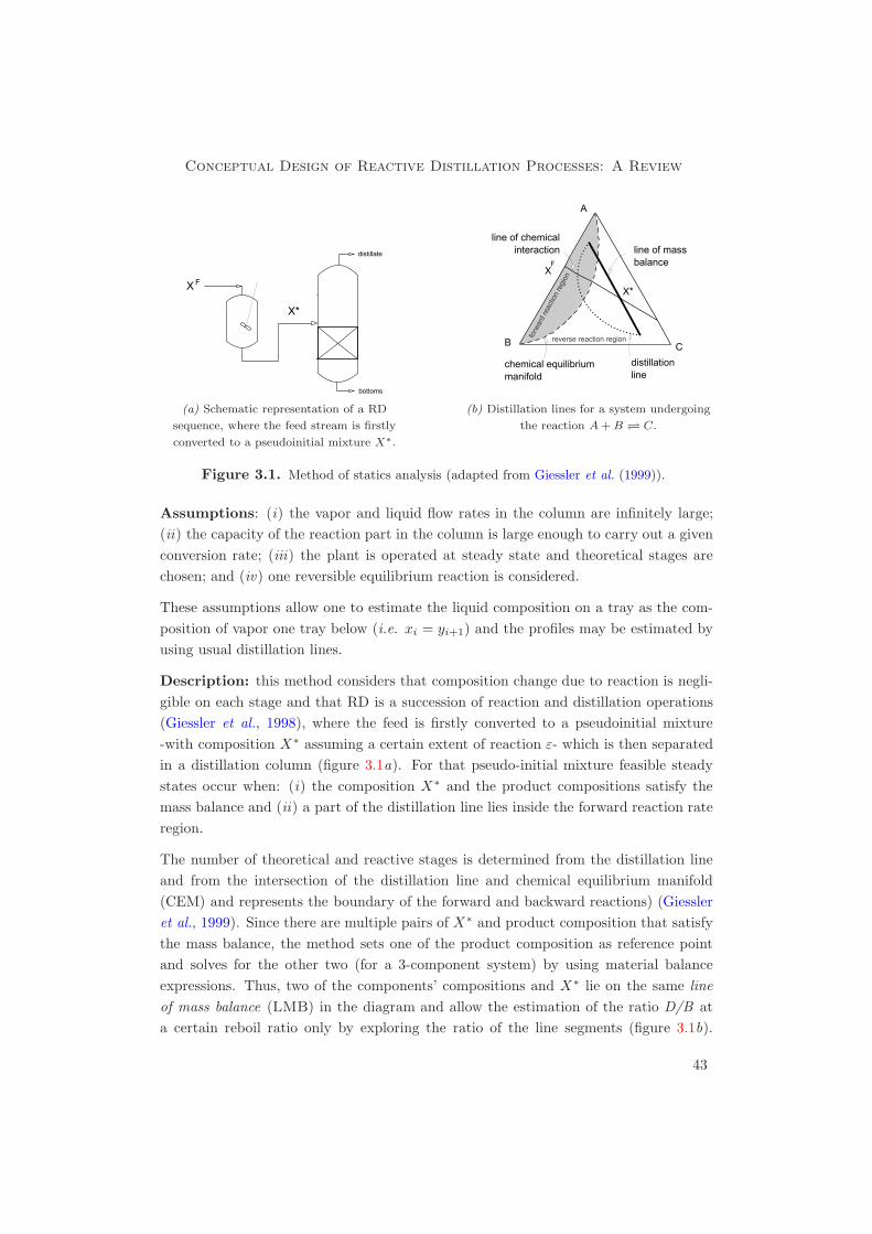
Conceptual Design of Reactive Distillation Processes: A Review
distillate
bottoms
X*
X F
(a) Schematic representation of a RD
sequence, where the feed stream is firstly
converted to a pseudoinitial mixture X∗.
A
B C
chemical equilibriummanifold
X
X*
line of mass balance
distillationline
line of chemicalinteraction
F
forw
ard
reac
tion
regi
on
reverse reaction region
(b) Distillation lines for a system undergoing
the reaction A+ B � C.
Figure 3.1. Method of statics analysis (adapted from Giessler et al. (1999)).
Assumptions: (i) the vapor and liquid flow rates in the column are infinitely large;(ii) the capacity of the reaction part in the column is large enough to carry out a givenconversion rate; (iii) the plant is operated at steady state and theoretical stages arechosen; and (iv) one reversible equilibrium reaction is considered.
These assumptions allow one to estimate the liquid composition on a tray as the com-position of vapor one tray below (i.e. xi = yi+1) and the profiles may be estimated byusing usual distillation lines.
Description: this method considers that composition change due to reaction is negli-gible on each stage and that RD is a succession of reaction and distillation operations(Giessler et al., 1998), where the feed is firstly converted to a pseudoinitial mixture-with composition X∗ assuming a certain extent of reaction ε- which is then separatedin a distillation column (figure 3.1a). For that pseudo-initial mixture feasible steadystates occur when: (i) the composition X∗ and the product compositions satisfy themass balance and (ii) a part of the distillation line lies inside the forward reaction rateregion.
The number of theoretical and reactive stages is determined from the distillation lineand from the intersection of the distillation line and chemical equilibrium manifold(CEM) and represents the boundary of the forward and backward reactions) (Giessleret al., 1999). Since there are multiple pairs of X∗ and product composition that satisfythe mass balance, the method sets one of the product composition as reference pointand solves for the other two (for a 3-component system) by using material balanceexpressions. Thus, two of the components’ compositions and X∗ lie on the same lineof mass balance (LMB) in the diagram and allow the estimation of the ratio D/B ata certain reboil ratio only by exploring the ratio of the line segments (figure 3.1b).
43

Chapter 3
After fixing the reference point, all the compositions of LMB are explored to estimatethe degree of conversion required in the reaction step. The highest conversion valueis found by iteration among the feasible degrees of conversion and defines the limitingsteady state (LSS) (i.e. condition of maximum conversion for a certain reactant (Giessleret al., 1999)). At this condition, the location and the length of the reactive zone inthe RD column are estimated by counting all reactive stages present in the forwardreaction section. Attaining the LSS can proceed by several limiting paths, dependingon the nature of the stability of the fixed point from which the distillation lines startor end. According to Giessler et al. (1998), if LSS is not convenient, the compositionof the initial mixture, the structure of the phase equilibrium diagram and the reactionsconditions (P, T ) have to be changed and the iteration loop is performed again. Theproposed method stresses the importance of identifying all feed composition regions,since they lead to the complete set of column configurations. Thus, the entire feedregion is classified into several sub-regions, each of which has the same characteristicswith respect to the product configurations (Giessler et al., 2001).
Advantages: this method (i) gives a straight forward solution to the question whetheror not a reaction should be performed in a RD column; (ii) allows one to synthesizeflowsheets qualitatively (e.g. maximum degree of conversion, reactive zone location andlength and column sequencing) (iii) for its application this method requires little data(i.e. feed composition, phase equilibrium model parameters, chemical equilibrium modelparameters and reaction stoichiometry); this method (iv) provides an effective tool forthe study of strongly nonideal mixtures with multiple chemical reactions and number ofcomponents; (v) allows the selection of the appropriate steady states from their completeset; (vi) simplifies troublesome calculations (including expensive full-scale experiments)reducing dramatically computational time (up to 5 times); (vii) represents a generalmethod that does not depend on the concrete column structure; (viii) does not requirethat product compositions, extent of reaction and number of stages are fixed a priori;and (ix ) allows one to determine the stability of various product regimes and derive thepossible product compositions and the column structure for one fixed feed compositionand the entire feed region.
Limitations: (i) this method assumes infinite separation efficiency; and (ii) matchingthe operating lines with the assumed product composition can be sometimes trouble-some.
3.2.2 Residue Curve Mapping Technique
The residue curve mapping (RCM) technique has traditionally been considered a pow-erful tool for flowsheet development and preliminary design of conventional multicom-ponent separation processes. It represents a good approximation of actual equilibrium
44

Conceptual Design of Reactive Distillation Processes: A Review
behavior and allows one to perform feasibility analysis of separation processes wherenonideal and azeotropic mixtures are involved (Siirola, 1996b,a; Malone and Doherty,2000). Furthermore, residue curves have been used to predict the liquid-compositiontrajectories in continuous distillation units in the ∞/∞ case (Barbosa and Doherty,1988a; Espinosa et al., 1996). Although for finite columns those profiles differ slightlycompared to the residue curves under same isobaric conditions (Fien and Liu, 1994),this difference is normally considered negligible at the first stages of design. A feasibilitycriterion may be derived from RCM considerations, where feasible composition profilesshould be enclosed by the total reflux profiles (i.e. residue curves) and the reversibleprofiles (i.e. profiles at the minimum reflux ratio) (Espinosa et al., 1999). Conceptu-ally, residue curve mapping is a phase equilibrium representation for systems involvingazeotropes (Siirola, 1996a,b) and qualitatively studies the behavior of a (non-) reactivemixture in a heated still. Analytically, RCM are constructed based on physical proper-ties of the system (i.e. vapor-liquid equilibrium, liquid-liquid equilibrium and solubilitydata), wherein the composition of a non-reacting liquid remaining in the system may bedetermined by performing overall and component material balances (Westerberg et al.,2000; Jimenez et al., 2000).
For multicomponent systems undergoing nrx equilibrium reactions, RCM are definedin terms of transformed molar compositions (Ung and Doherty, 1995a; Doherty andBuzad, 1992),
dXi
dτw= Xi − Yi, with Xi(0) = Xi,0, i ∈ Z
nc−nrx−1, (3.1)
with
dτw = dt×(
1 − νTtotal(Vref)−1yref
1 − νTtotal(Vref)−1xref
)× V/ML, (3.2)
Xi = xi−νTi (Vref)
−1xref
1−νTtotal(Vref)−1xref
, Yi = yi−νTi (Vref)
−1yref
1−νTtotal(Vref)−1yref
, i ∈ Znc−nrx , (3.3)
Vref =
ν(nc−nrx+1),1 · · · ν(nc−nrx+1),nrx
... νi,r
...νnc,1 · · · νnc,nrx
, (3.4)
where Xi and Yi are the transformed composition variables for the component i in theliquid and vapor phases respectively (i ∈ Z
nc−nrx), τw is a warped time, xref is the col-umn vector composed of the liquid molar compositions of the nrx reference components,Vref is the square matrix of stoichiometric coefficients for the nrx reference componentsin the nrx chemical reactions. Note that non-reference components ∈ [1, nc − nrx] andreference components ∈ [nc − nrx + 1, nc].
This new set of variables defines a sub-region of lower dimension in the compositionspace composed of the feasible product compositions for equilibrium controlled reac-tions. The RCM problem is solved by specifying the relation between the transformed
45

Chapter 3
compositions of the vapor and liquid phases and by using relevant properties of thetransformed compositions.
Description: (i) specify the compositions of the mixture charged to the pot (i.e.Xi,0 = Xe
i ); (ii) calculate composition of the equilibrium vapor; and (iii) calculate Yi
and integrate expression 3.1 until a singular point is reached (i.e. Xi = Yi).
For kinetically controlled reactions, an autonomous residue curve expression can bederived in terms of the Damkohler number (Da = kf,ref×ML
V ) and for the heating policyV/V0 = ML/ML
0 ,
dxi
dτw= xi − yi +Da× (νi − νtotal × xi)× kf
kf,ref× r, with xi(0) = xi,0, i ∈ Z
nc ,
(3.5)where ML
0 is the initial mass of liquid in the pot, V0 is the initial vapor flow, kf is therate constant for the forward reaction, r is the composition-dependent reaction rate, refdenotes the reference conditions of the system and dτw = dt× V × (ML)−1.
The influence of Damkohler number on the trajectory of the residue curves is evident.For Da=0 the residue curve lines will end in the highest boiling stable node (i.e. purecomponent or nonreactive azeotrope), whereas for high Da the lines will also end ina stable node, corresponding to a pure component, chemical equilibrium point or areactive azeotrope.
Advantages: (i) this method provides a reliable tool to perform feasibility analysisin RD; and (ii) for its application this method requires little data (e.g. feed compo-sitions, phase equilibrium model parameters, chemical equilibrium model parametersand reaction stoichiometry).
Limitations: (i) although relevant improvements have been made towards multiplecomponent (nc > 3) mixtures (Malone and Doherty, 2000), the RCM technique islimited by its intrinsic graphical nature; and (ii) accurate thermodynamic data arerequired to correctly describe the RD process (Barbosa and Doherty, 1988b).
RCM techniques have been used as feasibility tools to develop a generalized and sys-tematic design approach for reactive feeds outside conventional composition ranges(Almeida-Rivera and Grievink, 2002, 2004). For the synthesis of MTBE two sepa-ration sequences have been found that depend on the location of the reacting feed inthe composition space.
3.2.3 Attainable Region Technique
The concept of attainable region (AR) has been extensively employed in the synthesisof reactor structures (Feinberg, 1999) and successfully extended to processes combiningsimultaneous reaction, mixing and separation (Nisoli et al., 1997). In combination with
46

Conceptual Design of Reactive Distillation Processes: A Review
graphical methods, an activity based reaction-separation vector is defined, which satis-fies the same geometric properties as the reaction vector does. Therefore, it allows oneto construct the attainable region using the existing procedure for reaction-mixing sys-tems. In general terms and for a given system of reactions with given reaction kinetics,the AR may be defined as the portion of concentration space that can be achieved froma given feed composition by any combination of reaction and mixing (Nisoli et al., 1997;Gadewar et al., 2003). Thus, this technique aims to identify feasible reactor networks-albeit not the optimum- based on graphical properties of simple models of CSTR andPFR.
Assumptions: [Given: c1 and c2 are two attainable product compositions]: (i) everycomposition that lies on the segment line c1c2 belongs to the AR; (ii) on the ARboundary the reaction vector points inward, is tangent or is zero; and (iii) in thecomplement of AR no reaction vector intersects the AR.
Description: for the case of CSTR a component mass balance has been expressed interms of Damkohler number and the vapor fraction,
xi − xFi = φm
MW (xF )MW (y)
(xi − yi) +DaMW (xF )MW (x)
r(x)kf,min
(νi − νtotal × xi)︸ ︷︷ ︸RS(xi,yi)×Da
, i ∈ Znc ,
(3.6)where φm (≡ Vm/Fm) is the mass-based vapor fraction, Vm is the mass-based vaporflow, Fm is the mass-based feed flow, MW is the average molecular weight, Da is definedas Da = kf,min× ρm× υ/Fm, kf,min is the forward rate constant evaluated at the lowesttemperature on the boiling surface, ρm is the mass-based molar density, υ is the totalliquid volume, r(x) is the reaction vector, subscript m denotes mass-based values andRS(xi, yi) is the reaction-separation term.
For a PFR, the material balance is given by,
dxi
dη=
φm
Da
MW (xF )MW (yF )
(xi − yi) +MW (xF )MW (xF )
r(x)kf,min
(νi − νtotal × xi)︸ ︷︷ ︸RS(xi,yi)
, i ∈ Znc ,(3.7)
xi(0) = xi,0, i ∈ Znc , (3.8)
dη =MW (xF )MW (xF )
× kf,min × ρm
Lm(z)A(z)× dz, (3.9)
where A(z) is the cross sectional area of the PFR at the distance z ∈ [0, lPFR], lPFR isthe length of the PFR and η is a scaled time.
Expressions 3.6 and 3.7 are identical to those that describe the behavior of a CSTR andPFR and therefore, allow one to follow the same procedure for the construction of theAR (figure3.2).
47

Chapter 3
feed pointDa: parameter
Y
N
constructPFR and CSTR
trajectories
constructconvex hull
extend hull by using a PFR
RSpointing out
attainableregion
Figure 3.2. Procedure for the construction of attainable region. Nomencla-
ture: RS: reaction-separation term.
Advantages: (i) this method allows one to point out promising flowsheets; (ii) thereaction-separation vector has the same geometric properties as simple reactor models,allowing the application of the theory derived for PFRs and CSTRs; and (iii) thismethod can be easily extended to multiphase systems.
Limitations: (i) economic considerations are not taken into account to rank the designalternatives.
3.2.4 Fixed-Point Algorithm
A sound understanding on fixed points (cf. explanatory note 3.1) and the prediction oftheir behavior as a function of design parameters have been lately used as a design toolfor RD columns.
Assumptions: this technique is based on several assumptions, which depend on thenature of the contacting structure. Staged columns (Buzad and Doherty, 1994): (i)three component systems with a chemical reaction given by νAA + νBB � νCC; (ii)ideal vapor-liquid equilibrium; (iii) iso-molar reaction; (iv) negligible heat of reaction;(v) negligible heat of mixing; (vi) equal latent heats; and (vii) constant liquid hold-upon the reactive stages. Okasinski and Doherty (1998) removed these assumptions in thedevelopment of their more generalized design method. Packed columns (Mahajani andKolah, 1996): (i) applicability of the film theory of diffusion; (ii) uniform liquid com-position in the bulk; (iii) negligible axial dispersion/diffusion; (iv) CMO; (v) saturated
48
Conceptual Design of Reactive Distillation Processes: A Review
Fixed points At total reflux conditions, certain points in the concentration space are reached where
the composition on successive stages is constant (Buzad and Doherty, 1994, 1995) and in the
vicinity of which the columns profiles behave in a peculiar manner (Mahajani and Kolah, 1996;
Mahajani, 1999a). These fixed points occur at the pure component and azeotropic compositions
(Buzad and Doherty, 1994; Okasinski and Doherty, 1998) and move to new positions as the
reflux ratio (or external reboil ratio or Damkohler number) is changed. Fixed points can be
nodes (stable or unstable) or saddles and have a significant influence on the column composition
profiles, minimum reflux, etc. (Okasinski and Doherty, 1998). Unlike stable and unstable
nodes, the location of fixed points is dependent on process parameters and represents chemical
and physical equilibrium conditions. According to Espinosa et al. (1996), fixed points can be
obtained by finding tangents to residue curves that pass through the distillate or bottom streams.
In order to solve for the fixed-point compositions in terms of the Damkohler number -particularly
in terms of the critical value Dac- continuation methods are commonly used. These methods
involve solving the design equations for a range of Damkohler numbers, where the lower bound
corresponds to zero and the upper bound to the critical Damkohler number. The criterion for
fixed-point location establishes that for low Da the end of the profile will be located in the
negative reaction space (i.e. where the backward reaction is predominant), whereas for Da
above the critical value the end of the profile will be located in the positive reaction space. If
the balance expressions along the column are written as explicit finite difference equations (i.e.
xn+1 = f(xn, p)) the stability of the fixed points is determined by the eigenvalues λJ of the
Jacobian of f evaluated at the fixed points (Okasinski and Doherty, 1998).
Note 3.1. Fixed points in reactive distillation
liquid feed; (vi) negligible heat losses to the walls, heat of reaction and heat of mixing;(vii) total condenser; (viii) reboiler modelled as equilibrium stage with reaction; and(ix ) constant mass transfer coefficients, interfacial area and liquid hold-up.
Description: most of the pioneering work in the field of RD design for equilibriumcontrolled chemical reactions is based on transformations of the molar compositions byDoherty and co-workers (Barbosa and Doherty, 1987a,b, 1988a,b; Doherty and Buzad,1992; Ung and Doherty, 1995a,c). They devoted considerable effort in defining a designstrategy for equilibrium chemical reactions in staged columns. The resulting approachis based on the boundary value design method for nonreactive columns. It introducesa novel composition coordinate system, expressions 3.3, to transform the RD probleminto a form completely analogous to a non-RD problem, which may be solved usingconventional algorithms.
Similarly to the molar fractions, molar flow rates are transformed as suggested byGuttinger (1998),
ϑ = ϑ×(1 − νT
total × V−1ref × x
(ϑ)ref
), (3.10)
where ϑ denotes any of the streams present in the RD column (i.e. distillate, bottoms,feed, liquid and vapor flows) and ϑ represents the corresponding transformed value. Asmentioned by Frey and Stichlmair (1999b), the transformed compositions can be inter-preted as a projection of different chemical equilibrium states along their stoichiometric
49

Chapter 3
C
F'
B
i
A
F R
R'
(a) Non-transformed composition space.
i
BC reactive azeotrope
(b) Transformed composition space.
Figure 3.3. Dimension reduction through transformed compositions. Sys-
tems features: chemical reaction A+B + I � C + I ; where I is
an inert component (adapted from Frey and Stichlmair (1999b)).
lines (figure 2.2).
These definitions present convenient and simplifying properties: (i) the dimensionsof the system are reduced, simplifying the depiction of equilibrium (figure 3.3) (Freyand Stichlmair, 1999b; Barbosa and Doherty, 1987a); (ii) they have the same numericalvalues before and after reaction; (iii) they sum up to unity; (iv) they clearly indicate thepresence of reactive azeotropes whenXi = Yi; (v) the nonreactive limits are well defined;(vi) the number of linear independent transformed composition variables coincides withthe number of independent variables that describe the chemical equilibrium problem;and (vii) the lever rule is valid as the chemical reaction no longer impacts the materialbalance.
However, the introduction of transformed variables reduces the understanding of thephase equilibrium as a whole, hiding eventually some nonreactive azeotropes (Frey andStichlmair, 1999b).
For kinetically controlled reactions, the approach involves specifying all the degreesof freedom of the system and performing expanding envelope balances (material bal-ances around the rectifying, stripping sections and the entire column) from the endsof the column towards the middle (Buzad and Doherty, 1994; Huss et al., 1999). Themethodology is supported by the RCM technique (cf. chapter 5) and allows both afast screening for reactive azeotropes and feasible designs and the computation of thenumber of trays and the minimum reflux ratio (Ciric and Gu, 1994). If the target prod-uct compositions are feasible, the trajectories (for the rectifying and stripping sections)intersect. Then, for a given value of Damkohler there will be a single value of the reflux
50

Conceptual Design of Reactive Distillation Processes: A Review
ratio that satisfies the design equations (Doherty and Buzad, 1992). Intersection ofprofiles is a necessary but not sufficient condition. Thus, the accumulated extent ofreaction in the rectifying section plus that in the stripping section must be equal tothe initially assumed overall extent of reaction in the column (Okasinski and Doherty,1998),
D× xDi +B× xB
i − F × xfeedi
νi × F= (Darect ×
j=nrectt∑
j=1
MLj
ML0
kf,r
k0× rj)rect (3.11)
+(Dastrip ×j=nstrip
t∑j=1
MLj
ML0
kf,r
k0× rj)strip.
Fixed-point algorithm is not recommended by Ciric and Gu (1994) and Espinosa et al.(1996) for systems where the reaction kinetics, heat of reaction, liquid hold-up andresidence times are the determining design variables. However, Okasinski and Doherty(1998) successfully use it to reproduce the ethylene glycol synthesis example of Ciricand Gu (1994).
Mahajani and Kolah (1996) successfully extend the approach of Doherty and co-workersto packed columns, where liquid phase backmixing is totally absent. This approach relieson the performance of mass balances over differential elements of length dz in bothrectifying and stripping sections, which can be re-written as functions of dimensionlessnumbers (e.g. Da, HTU, dimensionless flux ϕi and ratio of characteristic times in thevapor and liquid sides β(≡ CV
total × kVm/C
Ltotal × kL
m))).
Rectifying section (i ⊂ {1, 3}):dyi
dζz= − ϕi
HTUV ,dxi
dζz=(
RR+1RR
) [− ϕi
HTUV +DaFV × g(x, T )
],
yi(0) = yi,0, i ∈ Znc , xi(0) = xi,0, i ∈ Znc .(3.12)
Stripping section (i ⊂ {1, 3}):dyi
dζz= − ϕi
HTUV ,dxi
dζz=(
RS+1RS
) [− ϕi
HTUV +Da FL+F × g(x, T )
],
yi(0) = yi,0, i ∈ Znc , xi(0) = xi,0, i ∈ Z
nc .
(3.13)
V-L equilibrium in the interface (i ⊂ {1, 3}):yi − ϕi = f(ϕi × β + xi), (3.14)
where ζz is the dimensionless height of the column and RR and RS are the reflux andreboil ratios, respectively.
The extent of reaction is given by,
εi =∫ zrect
0
ri × dz +∫ zstrip
0
ri × dz, i ⊂ {1, 3}, (3.15)
51

Chapter 3
where zrect and zstrip are the lengths of the rectifying and stripping sections, respectively.
The solution procedure reported by Mahajani and Kolah (1996) for packed columns isquite similar to that described by Buzad and Doherty (1994) for staged columns: (i)expressions 3.12-3.14 are solved simultaneously for various values of Da, determiningthe range where the stripping and rectifying profiles intersect; (ii) the satisfaction ofthe second necessary condition is then evaluated; and (iii) the sizing of the RD columnis performed.
Remarkable from Mahajani’s contributions is the parametric analysis of the design, interms of identifying the dependence of HTUV with Dac. It was concluded that forkinetically controlled reactions accompanied by slow mass transfer, the dimensionlessnumber (HTUV ×Dac) plays a mayor role in the feasibility of the design. Thus, profilesintersect if and only if (HTUV × Dac) falls in a specific range, whose width dependson the relative position of the fixed points (Mahajani, 1999b).
For RD columns where equilibrium controlled reactions are involved, the design method-ology follows the same guidelines developed by Barbosa and Doherty (1988a,b) forstaged columns. Thus, transformed variables can be introduced, reducing the dimen-sionality of the reactive system and simplifying the set of design equations.
It is revealed from this approach that the liquid hold-up has no direct influence on theperformance of the column, highly resembling the nonreactive distillation case. Fur-thermore, the reflux ratio is found to determine exclusively the feasibility of the design.Thus, for low reflux ratio values stable nodes are reached before the concentrationprofiles intersect (i.e. non-feasible design) whereas at high reflux ratios the profilesintersect and the design turns to be feasible. The value at which the profiles just touchcorresponds to the minimum reflux ratio. Although the parameters HTUV and β donot play a role in the intersection of the profiles, they determine the column height andthe extent of reaction.
Advantages: (i) this method is highly flexible in generating alternative designs atvarious design parameters (e.g. Damkohler number, reboil ratio or liquid hold-up inreactive zones) allowing one to put realistic bounds on those parameters (Okasinski andDoherty, 1998); and (ii) the mass and energy balances can be decoupled, allowing thedetermination of the column profile only using mass balance and equilibrium equations(Espinosa et al., 1996).
Limitations: this algorithm is limited by its inherent graphical nature, that imposespractical limitations and complicates its extension to systems where the number ofcomponents minus the number of independent stoichiometric reactions exceeds a valueof 3.
Fortunately, several modifications and extensions of the fixed-point method for stagedand packed columns are available in the open literature, aiming to relax part of the
52

Conceptual Design of Reactive Distillation Processes: A Review
assumptions on which the original algorithm was based. These relaxations include: (i)double feed columns (Okasinski, 1998); (ii) kinetically controlled reactions, which ac-count for the liquid hold-up in the column design and economics (Barbosa and Doherty,1988b, 1987a,b; Buzad and Doherty, 1994, 1995; Doherty and Buzad, 1992; Mahajani,1999a); (iii) multiple reactions (Ung and Doherty, 1995c); (iv) different hold-ups persection (Melles et al., 2000; Okasinski and Doherty, 1998); (v) heat effects (Melles et al.,2000; Okasinski and Doherty, 1998); and (vi) reactions where
∑vi �= 0 (Melles et al.,
2000; Okasinski, 1998).
3.2.5 Reactive Cascades
Chadda et al. (2003) and Gadewar et al. (2003) use the concept of reactive cascades toscreen the feasibility of hybrid RD systems. This approach has been successfully appliedto the preliminary design of single-feed and double-feed RD columns. The governingexpressions for the stripping (nstrip
t stages) and rectifying (nrectt stages) cascades are,
rectifying: yi,j−1 = φR,j × yi,j + (1 − φR,j)× xi,j − νi
(kf
kf,ref
)(D
1−D)r(xj)
i ∈ Znc−1, j ∈ [2, nrectt ].
(3.16)
stripping: xi,j−1 = φR,j × yi,j + (1 − φR,j)× xi,j − νi
(kf
kf,ref
)(D
1−D)r(xj)
i ∈ Znc−1, j ∈ [2, nstrip
t ],(3.17)
where φR,j = Vj
Lj−1is the fraction of feed L vaporized in the jth unit; and D is a
normalized Damkohler number (D = Da1+Da ).
Description: (i) for a given operating pressure, the feasibility diagram is drawn, whichis obtained by solving the component balances for the liquid/vapor molar compositionsin the stripping/rectifying sections. The independent variable φR,j is assigned a con-venient value, whereas D is used as parameter to move from equilibrium to kineticallycontrolled regimes; (ii) for a given D-value the column configuration (reactive or hybrid)is selected based on the satisfaction of the product specifications; (iii) the rectifying andstripping cascades expressions are solved at the given D-value until the fixed points arereached; (iv) depending on the column configuration, the stripping and/or rectifyingcascade expressions are solved for D=0; (v) the transformed compositions in the liq-uid/vapor phases are estimated according to expressions 3.3 for the stripping/rectifyingsections; and (vi) in the transformed composition space the lever rule is applied fora desired product composition. The design is deemed to be feasible if the lever ruleintersects both the rectifying and stripping cascade profiles.
Advantages: (i) a global feasibility analysis can be performed as a function of theproduction rate, catalyst concentration and liquid hold-up; (ii) this method does not
53

Chapter 3
have any restriction in the number of components or reactions; and (iii) this method isclaimed to be easily implemented.
Limitations: (i) the Damkohler number is assumed to be invariant on all the reactivestages; (ii) the effect of structural aspects of the unit (e.g. feed ratio type, location ofmultiple feeds, reflux and reboil ratios) are not considered; and (iii) the energy balancesare left out from the design methodology.
3.2.6 Thermodynamics-Based Approach
Stichlmair and co-workers (Frey and Stichlmair, 1999b; Stichlmair and Frey, 1999) studythe RD design from a thermodynamic-driven point of view. Their approach is based onthe existence of reactive distillation lines and potential reactive azeotropes (cf. §2.4).
Description: (i) the possible products (or feasible separation regions) are determinedfrom the knowledge of the existing concentration profiles within the column, whichin turn are represented by reactive distillation lines; (ii) the column mass balance isincluded; and (iii) possible separation borders are identified.
A thorough analysis of the behavior of reactive distillation lines with respect to thevolatility values of the involved components and the feed staging suggests the following(Bessling et al., 1997, 1998),
• RD is a feasible alternative for systems where the desired products are the nodesin a reactive distillation line diagram and their boiling points differ considerably,
• in the event that one of the desired products behaves as a saddle point, theconversion may be increased by adding a second feed stream in the column (e.g.synthesis of methyl acetate),
• the conversion of a two feed column reaches a maximum at finite reflux in thecase of products that behave as saddle points,
• RD is a feasible and cost-effective alternative if one of the desired products behavesas a saddle point and,
– high conversion is required at stoichiometric reactants ratio,
– separation between desired and undesired products is difficult,
– the boiling point difference between desired products is large,
– there is no distillation boundary line, and
– chemical equilibrium is on the side of the desired products (e.g. synthesis ofmethyl acetate).
54

Conceptual Design of Reactive Distillation Processes: A Review
Table 3.1. Combination of reactive and nonreactive sections (nrs) in a RD
column. (source: Bessling et al. (1997))
Reaction Inerts Desired products nrs
A � B A or B yesA � B C B/C yesA � B C A/C yesA � B C, D BC/D;BD/C;B/CD yesA � B C, D AC/D;AD/C;A/CD yesA+B � C C yesA+B � C A/B noA+B � C D C/D yesA+B � C D AD/B;A/BD noA+B � C+D A/B noA+B � C+D C/D no
• all components that need a reactant for the forward or backward reaction(s) arelocated in the low-dimensional reaction space,
• all inert components are located in the reaction space, and,
• if it is aimed to separate a product that is not present in the reaction space, anonreactive distillation section is required. Table 3.1 presents a general overviewfor the combination of reactive and nonreactive sections for several stoichiometries.
Advantages: (i) this approach can be applied to both fast and slow chemical equilib-rium reactions; and (ii) feasible products can be determined within a RD column.
Limitations: (i) finding the reactive azeotropes might be sometimes troublesome; and(ii) detailed knowledge of phase equilibrium, reaction kinetics and residence time withinthe column is required.
3.2.7 Conventional Graphical Techniques
These techniques allow the distribution of reaction zones within a column using theMcCabe-Thiele and Ponchon-Savarit methods for a given reaction conversion by ad-justing the catalyst hold-up on each stage. Although the methods are currently limitedto binary reactive mixtures, they provide fundamental insights towards multiple compo-nent systems. In general terms, it is suggested that if the reaction has a heavy reactantand a light product, the reaction zone should be placed in the rectifying section, whereasif the reaction has a light reactant and a heavy product, the reaction zone should belocated in the stripping section (Lee et al., 2000b,c,d).
Assumptions: (i) binary system with a single chemical reaction; (ii) CMO; and (iii)vapor-liquid equilibrium.
55

Chapter 3
Ponchon-Savarit method. This method is traditionally considered a powerful visu-alization tool for the synthesis of distillation columns for binary mixtures. Thus,it allows the designer to account graphically for the enthalpy effects that causea varying molar overflow when stepping off stages (Lee et al., 2000b). The mainissue of this approach is the definition of the reactive cascade difference point ,which for an exothermic isomerization reaction occurring in the rectifying zonemoves towards the reactant and downward as the calculation goes down the col-umn. The following nomenclature is adopted for the diagram coordinates (Leeand Westerberg, 2000),
δrectR,n =D× xD − cP× εn + cR× εn
D, (3.18)
hrectR,n =
hD + qc + ∆rH × εn
D, (3.19)
qc =Qcond
D, (3.20)
where δrectR,n and hrectR,n are the composition and enthalpy coordinates in the Ponchon-
Savarit diagram, D is the distillate flow, cP is the product coefficient vector, cR isthe reactant coefficient vector, εn is the sum of the extent of reactions occurring instages n and above, h is the liquid enthalpy, Qcond is the condenser duty and ∆rH
is the heat of reaction. It is concluded from this study that the number of reactivestages and the location of the feed stage are highly dependent on the extent ofreaction ε in the RD column. Thus, the determination of the optimal feed stage ispossible by connecting the bottom difference point and the final difference pointof the rectifying section, which in turn depend on the assumed extent of reactionon each stage (Lee et al., 2000b).
McCabe-Thiele method. This method is used to assess qualitatively the impact ofchanging a design variable (Lee et al., 2000c). For the RD case, two main featuresare tracked to sketch the diagram for a binary mixture of reactants undergoingan isomerization reaction and under CMO assumption,
• the intersection point of the operating line with the y = x line defines thereactive cascade difference point, which moves proportionally as the ratiomolar extent of reaction to product flowrate (i.e. xn = xD − εn/D); wheren denotes the stage number,
• the heat supplied by the reaction decreases the slope of the operating lineprovided that the location of the reactive cascade difference point is notchanged.
A simplified procedure for sketching the McCabe-Thiele diagram is depicted infigure 3.4 for an isomerization reaction.
56

Conceptual Design of Reactive Distillation Processes: A Review
assume totalextent of reaction
determine D and B
by material balance
assume top andbottom product
purities
constructq-line
choose a bottom purity above the purity of the
original feed
based upon feedcomposition and quality
assume an extentof reactionfor stage n
constructoperating line
passing through the newdifference point more reactive
stages
decide the optimalfeed tray location
intersect operaring linewith the stripping line
on the q-line
difference point does notmove anymore
switch between operatinglines leading to the
fewest stages
N
Y
n=n+1
move difference point
Figure 3.4. Procedure for sketching the McCabe-Thiele diagram. Systems
features: isomerization reaction of the type A � 2B (adapted
from Lee et al. (2000c)).
Advantages: (i) these methods allow a transparent visualization of tray-by-tray cal-culations; (ii) they might be fundamental tools for the conceptual design of RD column;and (iii) they allow one to visualize the impact of the location of the reactive sectionsand the feed location within the column.
Limitations:(i) these methods are exclusively applied to isomerization reactions; and(ii) they are limited by their inherent graphical nature.
3.2.8 Phenomena-Based Approach
According to this method -proposed by Hauan (1998)- three independent phenomenatake place simultaneously in a RD column: mixing, separation and reaction (Hauan andLien, 1996; Westerberg et al., 2000). These phenomena may be represented by vectors(figure 3.5) and allow the description of the total process profile of the system as a
57

Chapter 3
reaction
separation mixing
Figure 3.5. Schematic representation of the phenomena vectors in the com-
position space.
trajectory in the composition space for a control volume moving through a completesequence of process units.
Thus, each step along the profile may be represented by the vectorial addition of thephenomena vector mixture (
−→M), separation (
−→S ) and reaction (
−→R ),
dx
dt=
−→M +
−→S +
−→R, with x(0) = x0, (3.21)
where x is the phase composition and the phenomena vectors are given by,
−→M = M×
xfeed1 − x0
1
...xfeed
nc− x0
nc
,
−→S = S×
x1 − y1...
xnc − ync
,
−→R = R×
ν1 − x01 ×
∑νi
...νnc − x0
nc×∑
νi
,
(3.22)
where superscripts feed and 0 denote feed and initial values respectively, M is thelength of the mixing vector and is determined by the relative amount of material inthe streams being mixed, S is a matrix reflecting average mass transfer rates and Ris a scalar calculated from catalyst activity, hold-up, temperature and pressure. Eachvector has a unique local direction (i.e. process feasibility) and vector length (i.e.process efficiency). Vector directions are calculated by physical and chemical data only,whereas vector lengths depend on the operating parameters and design variables.
58

Conceptual Design of Reactive Distillation Processes: A Review
Description: any composition change in the system due to chemical reaction maybe represented by a straight line from the singular point, termed difference point (i.e.xs = ν/
∑ν), through the local composition x0 (Hauan et al., 2000b),
x = x0 + (xs − x0)× ε∑ν
n0 + ε×∑ν, (3.23)
where n is the total number of moles.
As the local compositions may be those of feeds and chemical reaction products, thecomposition in the desired point may be expressed as a normalized linear combinationof the reaction difference points and distillate-, bottoms- or feed-composition vectors.From expression 3.21, a kinetic fixed point occurs when the vectorial contributions ofthe nonzero phenomena balance each other,
dx
dt=
−→M +
−→S +
−→R = 0, with x(0) = x0. (3.24)
Fixed points, which become evident by the presence of flat concentration profiles forlarge portions of the column, are by no means desired in RD and indicate a weakdesign or operation. Therefore, several ways to move away from a fixed point in thecomposition space are suggested,
• altering the mixing vector: by changing process variables (e.g. reflux and reboilpolicies, external feeds and hold-ups),
• altering the reaction vector length: by manipulating process variables (e.g. cata-lyst density, hold-up) or by introducing nonreactive stages in the reactive zone,
• incorporating pumparound reactors: in order to avoid a counter-productive sepa-ration vector.
Advantages: (i) only physical and chemical data are required to estimate the phe-nomena vectors, which are independent of the structural design of the unit; and (ii) thisapproach allows the designer to assess independently the effect of equipment structureand operating policies on the composition change in RD.
Limitations: (i) although this method is driven by fundamental considerations, itsapplicability requires further studies.
3.2.9 Scalar/Vectorial Difference Points Technique
The concepts of reactive cascade and scalar/vectorial difference points in reactive cas-cades (cf. explanatory note 3.2) have been successfully applied by Hauan et al. (2000a);Lee et al. (2000a) and Lee and Westerberg (2000) in the design of RD processes.
59

Chapter 3
Reactive cascade difference points are defined as the combined points of stoichiometric coeffi-
cients vectors and product compositions. For the isomolar reaction 2R � P1+P2, the difference
points in the rectifying and stripping sections are given by,
δrectR,n = D×xD+2εn(cR−cP)D+2εn−2εn
,
δstripR,n = B×xB+2εn(cR−cP)B+2εn−2εn
,(3.25)
where the material balances are estimated as follows,
rectifying: Vn+1 × yn+1 = xn × Ln + (D + 2εn − 2εn)δrectR,n ,
stripping: Vs × ys = xs−1 × Ls−1 − (D + 2εs − 2εs)δstripR,s
(3.26)
where subscripts s and n denote the number of stages in the stripping and rectifying sections,
respectively. The difference points move parallel to the vector (cR−cP), in the direction defined
by the dominant chemical reaction.
Note 3.2. Reactive cascade difference points
Assumptions: (i) known top and bottom compositions; (ii) known reflux ratio; (iii)CMO assumption; and (iv) chemical reaction of the type 2R � P1 + P2.
Based on rigorous graphical considerations, the number and location of the reactiveand nonreactive stages is obtained. For the system studied by Lee and Westerberg(2000), the reaction conversion of the feed stage is found to be always larger than thatof any single stage in the rectifying and stripping sections. This situation allows oneto guarantee the conversion on the feed stage at any reflux ratio. The location of thebubble point curve with respect to the chemical equilibrium curve plays a key role in thefeasibility of the process within the stripping and rectifying sections. Thus, if the bubblepoint curve lies to the right of the reaction equilibrium curve, the rectifying section showsa better performance towards reactants’ conversion than that of the stripping section.In this case, the forward reaction always takes place and enhances the separation task.
This approach is tested in the gas-phase disproportionation of toluene and in the de-hydratation of methanol into water and dimethyl ether. In the first case study themost competitive configuration is reported to be the reaction zone in the stripping andfeed sections. The effect of the reaction equilibrium constant is analyzed in the secondexample, resulting in feasible configurations with a single reactive stage.
Description [for a given phase and reaction equilibria in a stage RD column]: (i)for a liquid phase chemical reaction at the operating pressure P draw the reactionequilibrium and the bubble point curves (for gas phase chemical reactions, the dewpoint curve should be drawn and an equivalent procedure should be followed (Lee andWesterberg, 2000)); (ii) specify the top and bottom compositions, reboil and refluxratios; (iii) step up/down from the feed stage to the top/bottom stage; (iv) fromgraphical considerations (according to expressions 3.25, 3.26 and phase equilibriumrelationship), the accumulated extents of reactions for stripping/rectifying sections aredetermined; (iv) the liquid composition on the tray is calculated; and (v) tray-by-tray
60

Conceptual Design of Reactive Distillation Processes: A Review
calculations are performed upwards/downwards until the calculated liquid compositionequalizes the top/bottom product composition.
3.3 Optimization-Based Methods
This second group of design methods is composed of those methodologies, which aresupported by the power of computational subroutines and take into account importantelements of an overall design strategy (e.g. types of phase equilibrium, number ofcomponents, occurrence or not of chemical reaction on a given stage) (Giessler et al.,1998). In this category, the work of Ciric and Miao (1994); Ciric and Gu (1994);Pekkanen (1995); Cardoso et al. (2000); Bessling et al. (1997); Seferlis and Grievink(2001); Bansal et al. (2000); Bansal (2000); Bedenik et al. (2001); Poth et al. (2001);Frey and Stichlmair (2001); Stichlmair and Frey (2001); Gumus and Ciric (1997) andGeorgiadis et al. (2002) compile the fundamentals of this design approach. This sectiongives an individual description of the methods and concludes with the advantages andlimitations of this design method category.
3.3.1 Mixed-Integer Nonlinear Programming (MINLP)
This method is particularly helpful to find fully or partially optimized solutions for RDdesign variables (Malone and Doherty, 2000). The objective function for the RD prob-lem is commonly composed of two basic terms: annual operating cost (e.g. consumptionof raw materials, steam and cooling water) and the annualized investment (i.e. column,internals, reboiler and condenser). The constraints are formed from the MESH equa-tions on each tray, material balances at the top and bottom of the column, kinetic andthermodynamic relationships and logical relationships between process variables andthe number of trays.
Assumptions: (i) the vapor and liquid phases are in equilibrium on each tray; (ii) noreaction takes place in the vapor phase; (iii) the liquid phase is always homogeneous;(iv) the enthalpy of liquid streams is negligible; (v) the heat of evaporation is constant;(vi) temperature dependence of the reaction rates can be expressed in Arrhenius form;and (vii) the cost of separating products downstream is given by an analytical function.
The solution to the RD problems results in the optimum number of trays, the optimalfeed tray location, reflux ratio, condenser and reboiler duties and liquid hold-ups on eachtray. Since the model contains both continuous (e.g. temperature and composition)and discrete (i.e. number of trays) design variables, it should be solved by MINLPoptimization technique.
Description: (i) a master sub-problem decomposition approach selects integer vari-ables (i.e. number of trays) in a master program; and (ii) an optimal column design is
61

Chapter 3
obtained with a fixed number of trays in the primal problem.
Due to their combinatorial nature, MINLP problems have been lately tackled usingevolutionary algorithms (e.g. genetic algorithm, simulated annealing and evolutionstrategies), which require only information regarding the objective function (Costa andOliveira, 2001). However, these novel approaches demand huge computational time andlack robustness when solving highly constrained problems.
Ciric and Gu (1994) present a MINLP-based approach for the design of RD columnsfor systems where multiple reactions take place and/or where reactive equilibrium orthermal neutrality cannot be assured. This method is based on the combination of arigorous tray-by-tray model and kinetic-rate-based expressions to give basic constraintsof an optimization model that minimizes the total annual cost. The major variablesare the number of trays in the column, the feed tray location, the temperature andcomposition profiles within the column, the reflux ratio, the internal flows within thecolumn and the column diameter.
Lately Poth et al. (2001) apply MINLP technique to the synthesis of MTBE and com-pare the optimal processes for the assumption of chemical equilibrium and kineticallylimitations. Their results show that the total cost of the kinetic column is higher thanthat of the equilibrium case. Cardoso et al. (2000) apply a simulated annealing-basedalgorithm to solve a non-equilibrium RD column in the synthesis of ethylene glycol.The results obtained from this approach coincide satisfactorily with those reported byCiric and Gu (1994) using commercial optimization packages. Pekkanen (1995) appliesa local optimization algorithm to take advantage of the large number of degrees offreedom (� 3 + nc) in the design of RD columns. In that study, the stage hold-upsand tray efficiencies are taken as optimization variables and the local optimum is foundby tracking the directions of the concentration vectors in successive stages. Frey andStichlmair (2001) optimize the RD column for the synthesis of methyl acetate in thekinetically controlled regime with respect to total annualized cost. Multiple feedingof reactants is allowed in the optimization routine leading to a decrease in the energydemand. Stichlmair and Frey (2001) design RD columns for the synthesis of MTBEand methyl acetate. Their starting point is the definition of the process superstructure,which in turn is derived from thermodynamic fundamentals (e.g. stoichiometric linesand lines of possible reactive azeotropes). A generalized modular representation forprocess synthesis is presented and extended by Papalexandri and Pistikopoulos (1996)and Ismail et al. (2001), respectively. That approach is supported by fundamental massand heat transfer principles, which allow the definition of a multipurpose mass/heattransfer module. The optimized combination of building blocks defines the process su-perstructure. The effectiveness of this steady state approach is tested in homogeneousand two phase-reactions, absorption/extraction and RD processes. Ismail et al. (2001)include Gibbs free energy-based driving forces as constraints to guarantee the feasibility
62

Conceptual Design of Reactive Distillation Processes: A Review
of the reaction/separation/RD processes. The design of RD units with VLL equilibriumis studied by Gumus and Ciric (1997). Their optimization problem is formulated as aMINL-bilevel exercise, whose underlying feature involves the development of a single-level optimization problem. The solution of the single-level problem is a lower bound forthe solution of the bilevel problem. The objective function is the Gibbs free energy oneach tray subjected to the mass, energy balances, constitutive expressions and integervariables defining the number of trays at the minimum total annualized cost.
3.3.2 Orthogonal Collocation on Finite Elements (OCFE)
MINLP has been found to be troublesome for units with large number of trays andfor the simultaneous design of more than one distillation unit due to the considerablecomputational time required for attaining the solution (Seferlis and Grievink, 2001).Furthermore, special attention must be paid in the MINLP model formulation and initialguesses outside the feasibility domain may lead into convergence difficulties. OCFEtechniques is suggested by Seferlis and Grievink (2001) for the design and optimizationof staged RD columns. This approach transforms the discrete number of stages inthe column into a continuous variable and treats the composition and temperature asfunctions of the position.
Assumptions: (i) complete mixing of each phase at each stage; (ii) constant liquidhold-up and no vapor hold-up at each stage; (iii) no liquid entrainment from stage tostage; (iv) adiabatic stages; and (v) thermal equilibrium between the liquid and vaporstreams leaving each stage.
Description: (i) the column is separated into sections; (ii) each column section is di-vided into smaller sub-domains (i.e. fine elements); (iii) for each fine element a numberof collocation points is specified, where the mass and energy balances are exclusivelysatisfied; (iv) the collocation points are chosen as the roots of the discrete Hahn familyof orthogonal polynomials; and (v) Lagrange interpolation polynomials are used withineach finite element to approximate the liquid- and vapor- component flow rates, thetotal stream flow rates and the liquid and vapor stream enthalpies.
In the study by Seferlis and Grievink (2001), the oscillatory behavior in the compo-sition space of highly-diluted components is circumvented by transforming the molarfractions of those components. Additionally, a second alternative is proposed, whereinert components with low concentrations are removed from the energy and mass bal-ances. Both approaches are found to increase the stability and robustness of the solutionat the same level of accuracy. This technique is successfully applied to the design ofa RD column for the synthesis of ethyl acetate (Seferlis and Grievink, 2001), using asingle element with four collocation points in the rectifying section, three elements withthree collocation points per element in the reactive section and two elements with two
63

Chapter 3
collocation points per element in the stripping section. The study concludes that theproduction of ethyl acetate is strongly favored by large liquid-stage hold-ups in the reac-tive and stripping sections because of the relatively low rate of reactions. Furthermore,a double-column production flowsheet is selected, which allows the production of highpurity ethyl acetate.
3.3.3 Mixed Integer Dynamic Optimization (MIDO)
In general a chemical process that shows poor ability of meeting control objectives givesrise to missing opportunities with respect to economic performance and satisfaction ofproduct specifications. This fact may imply the existence of a trade-off between thoseprocesses designed with respect to control performance considerations and those drivenby economic issues. In order to circumvent this duality, relevant improvements are re-cently done towards the integration (Russel et al., 2000) and simultaneous optimization(Georgiadis et al., 2002; Bansal, 2000; Bansal et al., 2000) of the design and controltasks. The general design and control problem (cf. explanatory note 3.3) involves find-ing parameters (continuous and/or integers) that define the RD column and controltuning parameters at the minimum economic cost and with an acceptable dynamic per-formance in the presence of disturbances. The continuous parameters include columndiameter, reboiler and condenser areas and tuning parameters (gain K, set-point SPand reset time τc), while integer variables -y- involve the existence or not of catalyston a given stage (fk
rx ∈ {0, 1}). According to Georgiadis et al. (2002), the simulta-neous approach takes advantage of the interactions between design and control andprovides a fully operational process design that is cheaper and more controllable thanthat generated by the sequential approach.
Description: (Bansal et al., 2000; Bansal, 2000; Georgiadis et al., 2002) (i) set thetermination tolerance, ε; initialize the iteration counter, k = 1; lower bound, LB = −∞;and upper bound, UB = ∞; (ii) for fixed values of the integer variables, y = yk,solve the kth primal problem to obtain a solution, Jk. Omit the search variables andconstraints that are superfluous due to the current choice of integer variables. SetUB = min(UB, Jk) and store the continuous and integer variables corresponding tothe best primal solution; (iii) solve the primal problem at the solution found in step(ii) with the full set of search variables and constraints included. Convergence will beachieved in one iteration. Obtain the Lagrange multipliers needed to construct the kth
master problem; (iv) solve the kth master problem to obtain a solution ηk. Update thelower bound, LB = ηk; and (v) if UB − LB ≤ ε, or the master problem is infeasible,then stop. The optimal solution corresponds to the values stored in step (ii). Otherwiseset k = k + 1, yk+1 equal to the integer solution of the kth master problem and returnto step (ii).
64

Conceptual Design of Reactive Distillation Processes: A Review
Mixed-Integer Dynamic Optimization Problem
Obj.: minzp,zc,y
J(x(tf ), u(tf ), d(tf ), y(tf ), pp(tf ), pc(tf ), zp, zc, y, tf ),
s.t. 0 = f(x(t), x(t), u(t), d(t), y(t), pp(t), pc(t), zp, zc, y), t ∈ [t0, tf ]
0 = g(xd(t), xa(t), u(t), d(t), y(t), pp(t), pc(t), zp, zc, y), t ∈ [t0, tf ]
0 ≥ h(x(t), u(t), d(t), y(t), pp(t), pc(t), zp, zc, y), t ∈ [t0, tf ]
0 ≥ i(x(0), u(0), d(0), y(0), pp(0), pc(0), zp, zc, y), t ∈ [t0, tf ],
zp ∈ Zp, zc ∈ Zc, y ∈ [0, 1]
pp(t) ∈ P p ⊆ Rpp, pc(t) ∈ P c ⊆ Rpc
t ∈ [t0, tf ]
x(t) ∈ X ⊆ Rx, x(0) ∈ X ⊆ Rx,
(3.27)
where the objective function J(·) represents the overall cost of the RD processes (i.e. capital and
operational costs), the equalities f(·) and g(·) comprise the differential and algebraic expressions,
respectively; h(·) represents the path constraints that must be satisfied at all times during the
system operation, i(·) is the set of initial conditions, x denotes the set of state variables, u is the
set of input variables, y is the set of output variables, d is the set of disturbance variables, pp
and pc are the sets of time-varying variables for the process and control scheme, respectively; zp
and zc are the sets of time-invariant parameters for the process and control scheme, respectively;
and y is the set of integer variables.
Note 3.3. Mixed-integer dynamic optimization problem formulation (Bansal
et al., 2000; Bansal, 2000).
Advantages: (i) optimization-based approaches are applicable for multiple reactionsand where reactive equilibrium or thermal neutrality cannot be assured; and (ii) itallows the generation of optimum designs with respect to economics and controllability.
Limitations: (i) special care should be paid to the model formulation and the physicalsignificance of the solution; scaling of optimization variables might be required to reducecomputational effort; (ii) the optimization problem might be difficult to solve; (iii)huge computational time can be required for multiple alternative optimizations; (iv)it is difficult to perform sensitivity analysis of the optimum solution; and (v) locallimitations can be found when the initial guess lies outside the feasibility region.
3.4 Evolutionary/Heuristic Methods
A third trend of conceptual design approaches may be identified from the evolution ofRD as a derivation from conventional distillation processes. As stated by Subawalla andFair (1999), residue curve map techniques and fixed-point algorithms have been tradi-tionally very useful tools for preliminary screening and design of RD systems. However,they cannot be used for detailed design, since they rely on several limiting assumptionsand do not account for the special nature of reactive column internals. Those authorspropose a post -design algorithm to estimate parameters such as column pressure, reac-tive zone location, catalytic mass, reactant feed location, reflux ratio, column diameter,number of equilibrium stages and packed height. Moreover, the feasibility of up-stream
65
Chapter 3
pre-reactor is taken into account. For equilibrium-limited reactions, the following issuesare addressed (Subawalla and Fair, 1999),
• use of a pre-reactor: incorporating a pre-reactor could profitably enhance theconversion of equilibrium-limited reactions, especially when it handles a substan-tial part of the reaction duty.
� Rule of thumb 1: use a pre-reactor when reaction rate at 80% conversion ismore than half the initial rate.
• operating pressure: the column pressure ranges from the condenser pressure(determined by the condenser coolant temperature) to the reboiler pressure (fixedby the heating medium temperature and the column pressure drop). In generalterms and within this range, the operating pressure depends on the reaction tem-peratures, relative volatility and the effect of pressure on azeotropes. An upperpressure limit exists beyond which rates decrease because of reaction depletion dueto relative volatility and/or azeotropic effects and due to departure from chemicalequilibrium.
• reactive zone location: this parameter represents the best trade-off betweenconversion and product purity. For instance, when the limiting reactant is themost volatile component and the product is the heaviest component, the reactivezone is located towards the top of the column. For high purity requirements,stripping or rectifying sections must be incorporated either below or above thereaction zone.
� Rule of thumb 2: a reactive zone section should be located where the concen-tration of at least one reactant (preferably the limiting reactant) is the maximum.
• feed location: a right choice of feed location guarantees high concentrations ofreactants in the reactive zone, as shown in figure 3.6 for the synthesis of methylacetate. The following rules of thumb might be suggested:
� Rule of thumb 3: if the reactants are the most volatile components, thenthe feed should be introduced at the bottom of the reactive zone,
� Rule of thumb 4: if the volatilities of the reactants are very different, anadditional feed location may be required to ensure stoichiometric reactant quan-tities
� Rule of thumb 5: a pre-reacted product-containing feed enters the column atsome distance from the reactive zone, ensuring thereby that separation betweenreactants and products takes place on stages between the feed point and thereactive zone.
66

Conceptual Design of Reactive Distillation Processes: A Review
0 5 10 15 20 25 30
50
60
70
80
90
100 MeOH 6 HAC 19 MeOH 13; HAC 13 MeOH 12; HAC 14 MeOH 8; HAC 17
Con
vers
ion
of H
AC
[%]
Reflux ratio [-]
Figure 3.6. Influence of feed location on reactant conversion. Systems fea-
tures: synthesis of methyl acetate from methanol and acetic acid.
Legend: the numbers in the data series denote the feed tray loca-
tion from the top of the column. Conversion reaches a maximum
when the feed flows are located directly below and above the reac-
tive section of the column. (adapted from Bessling et al. (1998)).
• reactant ratio: reactants’ requirements can be calculated from product spec-ifications, desired conversion and azeotropic compositions at different operatingpressures.
• catalyst mass: the minimum catalyst requirements are determined by simulatinga series of isothermal PFRs and ideal separators in series. As depicted in figure3.7, the feed to the first PFR contains the necessary quantity of unconverted re-actants; the partially reacted effluent is fed to an ideal separator that completelyseparates reactants from products. This procedure is repeated for different tem-peratures until the desired conversion is reached, where the operating temperaturedefines the minimum amount of catalyst. Since there is a relevant influence of op-erating temperature on catalyst life, chemical equilibrium and column pressure,the adopted operation temperature value differs from the highest possible value.In order to account for the non-isothermal operation and for the imperfect sep-aration on each stage, the mass of catalyst should be 20-30% greater than theestimated value. Additionally, inadequate catalyst volume reduces residence timeand gives poor conversion.
• number of theoretical stages: the number of stages may be estimated to
67

Chapter 3
...
Figure 3.7. Column internals’ driven design: ideal reactor-separator train for
the estimation of minimum catalyst requirements. The partially
reacted effluent is fed to an ideal separator that completely sepa-
rates reactants from products.
0 2 4 6 8 10
40
50
60
70
80
90
100
Con
vers
ion
of A
[%]
Reflux ratio
Figure 3.8. Relation between conversion and reflux ratio for a RD column.
Systems features: chemical reaction A + B � C + D; compo-
nents volatilities: A/B/C/D = 4/1/8/2. (adapted from Bessling
et al. (1997)).
a certain extend by short-cut methods (e.g. Fenske Underwood), especially forthe nonreactive zones (stripping and rectifying). Note that there is an optimumnumber of reactive stages, which allows one to obtain the highest reaction extentfor given vapor flow and column height (Solokhin and Blagov, 1996).
• reactive zone height and column diameter: the diameter of the column isdetermined by the flooding velocity, vapor-liquid traffic, pressure-drop and pack-ing catalyst density; the reactive zone height, on the other hand, depends on thecatalyst mass, packing catalyst density and column diameter.
• reflux ratio: in RD columns, the rate and ratio of reflux play an importantrole in reaction and separation phenomena. For equilibrium-controlled systems,a high reflux rate increases the separation of products from reactants, therebyincreasing the reaction driving force. As noted in figure 3.8, excessive reflux leads
68

Conceptual Design of Reactive Distillation Processes: A Review
x feed , x B, x D RRmin vvapor, vliquid Dcol
Vcat , hcat, Ncat
Simulation
.
x decreasesRR 0.9 . RRvvapour, vliquid, Dcolx changes
mcat mcat. f (f<1)x= x desired
RR 0.9 .RR
Y
NY
N
N
Y
cat
catcat
col
catcatpack
catcat HETP
hN
D
Vh
mV === ;
4
;2
RR 1.1 RR
Figure 3.9. Procedure to estimate reactive zone height, reflux ratio and col-
umn diameter for a catalytic distillation column (adapted from
Subawalla and Fair (1999)).
to operating problems and insufficient reaction hold-up, leading to incompleteconversion.
� Rule of thumb 6: use a factor of 1.2-1.4 × the minimum ratio.
Short-cut methods derived from conventional distillation have been found to beinappropriate for the estimation of reflux ratio for reactive case and new ap-proaches have been adopted. Methods derived from the boundary-value approach(cf. §3.2.4) allow the determination of the minimum and real reflux ratio, whichare key factors in the determination of vapor and liquid velocities. The refluxratio can be calculated using an iterative procedure, described in Subawalla andFair (1999) and summarized in figure 3.9.
• reboil ratio: the feasibility of RD processes has been closely related to theminimum reboil ratio (RSmin), at which the composition of the rectifying fixedpoint equals the composition of the stripping fixed point (Okasinski and Doherty,1998). The reboil ratio normally ranges from 3 to 8 and reaches a minimum whenplotted versus the total number of stages.
• actual trays/packed height: For the stripping and rectifying sections experi-mental tray efficiency or packing HETP should be used, whereas for the reactivesection mass-transfer coefficients should be calculated from experimental data atthe operating conditions of the system. In the event that thermo-physical data,
69

Chapter 3
transport phenomena data and hydraulic models are available, non-equilibriumdesign approaches are found to provide a better agreement between experimenta-tion and simulation.
The proposed approach may be extended by incorporating hydraulic models which ac-count for the column capacity in terms of pressure drop and for mass-transfer efficiencyestimations in terms of liquid hold-up, mass-transfer coefficients and interfacial area.
Advantages: this method estimates easily several equipment and/or operational vari-ables.
Limitations: this method is basically a post-design algorithm and as such it requiresan already defined process structure.
3.5 Concluding Remarks
Both the graphical and optimization-based design methods have already proven theirpotential in RD process design but have also shown some significant limitations. Graph-ical methods are fairly flexible in generating alternative designs at various design pa-rameters, allowing the designer to define realistic bounds on them. Furthermore, thegraphical nature of the methods clarifies the understanding of those fundamental issuesin RD, which might be disguised by other approaches (e.g. reactive azeotropes). Onthe other hand, graphical methods are strongly limited by their graphical nature (i.e.(nc − nrx) ≤ 3). Optimization-based methods overcome the last limitation and havesuccessfully solved design problems, where multicomponent mixtures, multiple chemicalreactions and multiple units are involved. However, additional caution is required in theproblem formulation and inappropriate initial guesses of the optimization variables maylead into convergence difficulties. The evolutionary method proposed by Subawalla andFair (1999) covers in more detail some physical aspects of the design of RD columns.However, this approach requires a pre-defined structure and accordingly the optimumdesign is not guaranteed.
Based on their assumptions, limitations and outputs a fingerprint chart was produced forthe methods described in this chapter. From this qualitative plot (table 3.2) the follow-ing conclusions can be drawn: (i) most of the graphical methods provided fundamentalinsights on the feasibility of the RD process and define the initial process structure; (ii)economic considerations are taken into account exclusively by optimization-based meth-ods; (iii) the availability of the process has not been included as design output by anymethod, since this temporal feature is normally dealt at the next level of engineeringdesign; (iv) the heuristic-based methodology is based on an already designed processand is therefore a post-design tool; (v) most of the design methods have been developedfor steady state operation; (vi) the initial effort required for optimization-based meth-
70

Conceptual Design of Reactive Distillation Processes: A Review
ods is far more significant than that for graphical approaches, but the output generatedby the programming-based design is more comprehensive.
Due to the size and conceptual/computational complexity of the RD design problem, asingle comprehensive design strategy might not be available for years to come. Almeida-Rivera and Grievink (2001); Almeida-Rivera et al. (2004a), however, propose an inte-grated design approach -termed multiechelon design approach. This strategy allows thedesigner to combine in a systematic way the capabilities and complementary strengthsof the available graphical and optimization-based methods. As discussed in detail inthe course of the coming chapters, this approach is supported by a decomposition in ahierarchy of imbedded design spaces of increasing refinement. Moreover, it constitutesthe framework of a highly aggregated design methodology, which focuses on the RDdesign problem from a life-span perspective.
Mind journey to the scientific questions.
If we take a mind journey back to the engineering/scientific de-sign question given at the beginning of this chapter, the followingremark can be made. An overview and analysis of representa-tive design methodologies are provided in this chapter. Based onidentified opportunities, an integrated design approach is brieflymentioned, which offers the benefit of combining the capabilitiesand complementary strengths of available methodologies. Thedomain knowledge in RD design is addressed. Therefore, the ma-terial presented in this chapter contributes to the answering ofQuestion 4.
71

Chapter 3
Table 3.2. Qualitative fingerprint of the design methods used in reactive
distillation. Nomenclature. G1: Statics analysis; G2: RCM;
G3: Attainable region G4: Fixed-points; G5: Reactive cascade;
G6: Thermodynamic-based; G7: Conventional graphic techniques; G8:
Phenomena-based; G9: Difference points; M1: MINLP; M2: OCFE;
M3: MIDO; H1: Heuristics. Key. �: applicable; �: nonapplica-
ble/nonmentioned; �: original assumption relaxed by later contributions
G1 G2 G3 G4 G5 G6 G7 G8 G9 M1 M2 M3 H1
Inputphase equilibrium model � � � � � � � � � � � � �chemical reaction equilibrium � � � � � � � � � � � � �chemical reaction kinetics � � � � � � � � � � � � �feed compositions � � � � � � � � � � � � �compositions of product streams � � � � � � � � � � � � �reboil/reflux ratios � � � � � � � � � � � � �initial spatial superstructure � � � � � � � � � � � � �type packing/hydrodynamic features � � � � � � � � � � � � �temporal disturbance scenario � � � � � � � � � � � � �Knowledge requiredModel assumptionsphase equilibrium � � � � � � � � � � � � �negligible heat effects � � � � � � � � � � � � �equilibrium controlled regime � � � � � � � � � � � � �kinetically controlled regime � � � � � � � � � � � � �steady state operation � � � � � � � � � � � � �multicomponent systems (≤ 3) � � � � � � � � � � � � �single reaction � � � � � � � � � � � � �constant molar overflow � � � � � � � � � � � � �constant liquid holdup � � � � � � � � � � � � �isomolar stoichiometry � � � � � � � � � � � � �negligible axial dispersion � � � � � � � � � � � � �constant volatilities � � � � � � � � � � � � �infinite vapor/liquid flows � � � � � � � � � � � � �film theory validity � � � � � � � � � � � � �constant mass transfer coefficients � � � � � � � � � � � � �Rulesconnectivity, units’ selection � � � � � � � � � � � � �operating conditions � � � � � � � � � � � � �Outputfeasibility of the RD process � � � � � � � � � � � � �definition process superstructure � � � � � � � � � � � � �
Continue in next page
72

Conceptual Design of Reactive Distillation Processes: A Review
Table 3.2. Qualitative fingerprint of the design methods used in reactive dis-
tillation (continuation). Nomenclature. G1: Statics analysis; G2:
RCM; G3: Attainable region G4: Fixed-points; G5: Reactive cascade;
G6: Thermodynamic-based; G7: Conventional graphic techniques; G8:
Phenomena-based; G9: Difference points; M1: MINLP; M2: OCFE;
M3: MIDO; H1: Heuristics. Key. �: applicable; �: nonapplica-
ble/nonmentioned; �: original assumption relaxed by later contributions
G1 G2 G3 G4 G5 G6 G7 G8 G9 M1 M2 M3 H1
operating conditions (reflux, reboil) � � � � � � � � � � � � �number of (non-) reactive stages � � � � � � � � � � � � �location feed stages � � � � � � � � � � � � �location (non-) reactive azeotropes � � � � � � � � � � � � �determination MSS � � � � � � � � � � � � �Life-span perspectiveeconomic considerations � � � � � � � � � � � � �exergy efficiency considerations � � � � � � � � � � � � �controllability considerations � � � � � � � � � � � � �Nature of outputstructure � � � � � � � � � � � � �performance (economics) � � � � � � � � � � � � �physical behavior (operability) � � � � � � � � � � � � �physical behavior (availability) � � � � � � � � � � � � �Effortmodel complexity � � � � � � � � � � � � �implementation time � � � � � � � � � � � � �tools’ complexity � � � � � � � � � � � � �
Coming from previous page
73


“A problem clearly stated is a problem half solved.”
Dorothea Brande, ‘Becoming A Writer ’ (1934)
4A New Approach in the Conceptual Design
of Reactive Distillation Processes†
The potential benefits of applying RD processes are taxed by significant complexities
in process development and design. Several topics regarding these two activities are
addressed in this chapter. The interactions between process development and design
activities are considered first. The RD design problem is then formulated in the
wider context of process development and engineering. The identification of requested
output information from current methodologies results in the introduction of a set
of performance criteria SHEET (safety, health, environment, economics, technology).
The focus is on the design problem from a life-span perspective. A multiechelon
approach is subsequently introduced, in which a hierarchy of embedded design spaces
of increasing refinement is used and the strengths of current design methods are
conjugated.
†Parts of this chapter have appeared in Almeida-Rivera et al. (2004a) and Almeida-Rivera and
Grievink (2001)
75

Chapter 4
4.1 Introduction
When chemical reactions and physical separations have some overlapping operatingconditions the combining of these tasks into a single process unit can offer significantbenefits. These benefits may involve: avoidance of reaction equilibrium restrictions,higher conversion, selectivity and yield, removal of side reactions and recycling streams,circumvention of nonreactive azeotropes and a reduction in number of units (i.e. in-vestment cost) and energy demands (i.e. heat integration) (Schembecker and Tlatlik,2003; Subawalla and Fair, 1999; Stichlmair and Frey, 1999; Jimenez et al., 2001; Maloneand Doherty, 2000). However, there is a price to pay in terms of increased complexityin design and operations. The nonlinear coupling of reactions, transport phenomenaand phase equilibria can give rise to highly system-dependent features, possibly leadingto the presence of reactive azeotropes and/or the occurrence of steady-state multiplici-ties. The number of design decision variables for such an integrated unit will be high.Industrial relevance requires that design issues are not separated from the context ofprocess development and plant operations. Hence, the design problem is addressed inthis chapter from a process life-span perspective.
The starting point of this approach is the qualitative analysis of current design method-ologies in RD presented in chapter 3. Table 3.2 clearly shows the complementary as-pects of the graphical, programming-based and heuristic-based methods. The graphicalmethods are capable of generating feasible process structure options under somewhatidealized chemical and physical conditions. Optimization-based methods, once givena superstructure, can generate more detailed and complete designs from an engineer-ing perspective and can even be used to strive to account for controllability aspects.Heuristic-based methodologies provide only rough estimates of the design variables andrequire a pre-defined process structure.
The complexity and full range of design variables in process integrated RD units are, asyet, not considered in the scope of the current RD design methods. Process integrateddesigns should take into account the economic and exergy-related interactions of theRD units with the process surroundings and comply with the desired dynamics andcontrol of the overall process supply chain.
In view of the size and of the conceptual and computational complexity of a RD designproblem, a single comprehensive design technique is unlikely to become available forsome years to come. An integrated design strategy (Almeida-Rivera and Grievink,2001; Almeida-Rivera et al., 2004a) is introduced in the forthcoming sections. Thisdesign strategy allows the designer to combine, in a systematic way, the capabilities andcomplementary strengths of the available graphical and optimization-based methods.This integrated approach is embedded within a highly-aggregated design methodology,which is characterized by a set of performance criteria. In clear agreement with a life-
76

A New Approach in the Conceptual Design of RD Processes
span perspective (cf. explanatory caveat in section §1.4) these criteria account for theeconomic, exergy-related and temporal performance of a design focussed on preventionof loss of resources.
It is worth mentioning here that the present contribution focuses on the definition ofthe RD process structure, paying less explicit attention to a detailed analysis of theactual dynamics of the unit, which might be described using non-equilibrium models.An extended review on this last topic can be found in the publications of Taylor andKrishna (2000); Krishnamurthy and Taylor (1985); Taylor and Krishna (1993, 2003).Furthermore, the temporal features of the process unit(s) (e.g. operability and avail-ability) are not fully considered in the proposed methodology, as availability is foreseento be taken into account at the next level of engineering detail.
Recalling the engineering and scientific design questions given in chapter 1, in thischapter we address question 5, namely,
• What are the (performance) criteria that need to be considered from a life-spanperspective when specifying a reactive distillation design problem?
4.2 Interactions between Process Development and Process
Design
The aim of chemical process design has, conventionally, been considered as the findingof equipment sizes, configurations and operating conditions that will allow for the eco-nomical, safe and environmental responsible conversion of specific feed stream(s) intospecific product(s). This task is in principle carried out only by specifying the stateof the feeds and the targets on the output streams of a system (Doherty and Buzad,1992; Buzad and Doherty, 1995). Frequently, however, the design activity is found to beseverely complicated by the difficulty of identifying feasible equipment configurationsand ranges of suitable operating conditions. This situation can be explained by the factthat the design of chemical process units is only a constitutive part of a larger scale and,therefore, more complex problem: the joint consideration of process unit developmentand design. At this higher level of aggregation, the objective of the design problemincludes sizing the unit and establishing the requirements of the design, screening theprocess feasibility and, at the top, identifying the process opportunities (figure 4.1).
From this point of view, two parallel and inter-related activities can be identified: thedesign program and the development program. For a given level of design detail all thedesign tasks should be considered from top (i.e. higher aggregation/process level) tobottom (i.e. low aggregation/unit level). The information leaving the design programis compared with the desired outputs. If an acceptable agreement exists the level ofdetail is increased and the same strategy is adopted. For non-acceptable outputs the
77

Chapter 4
Identify opportunities
Screen feasibility
Design requirements
Design of units
input data
assumptionsmodels
strategies
decr
easi
ng a
ggre
gatio
n le
vel
refineddesign level
redefinitionimprovementreformulation
i ncreasing detail levelDESIGN PROGRAM
PROCESS DESIGN
desired output
Y
N
agreement ?
DEVELOPMENT PROGRAM
design/perform experimentmethod development
Improved knowledge
Figure 4.1. The design problem regarded as the combination of a design pro-
gram and a development program.
loop is performed at the same level of detail after redefining/reformulating appropriateassumptions/models/generalities in the design program. This is attained by designingand performing an appropriate development program, which allows the designer toextend/improve/correct the existing knowledge and methodology (e.g. removing theuncertainties introduced by estimation of parameters).
Within the design program, the following design tasks are defined.
Identification of opportunities. This task permits one to select qualitatively the setof competing process technologies/equipment configurations, which might be usedto convert the given feeds to the desired products. Schoenmakers and Bessling(2003b), for instance, use the physical/chemical characteristics of the system (e.g.reaction velocity and relative volatility) to choose the equipment configuration.Proven technologies together with novel configurations might arise at this stage(e.g. dividing wall columns, pump-around reactors, side-reactors, etc.) (Baur andKrishna, 2003; Krishna, 2003; Mutalib and Smith, 1998a,b).
Screening of feasibility. The feasibility of the selected opportunities is then screenedwith respect to the attainable products of a given set of feed streams. In this stagethe concepts of attainable region (Feinberg, 1999; Nisoli et al., 1997) and ∞ / ∞approach (Westerberg and Wahnschafft, 1996; Fien and Liu, 1994; Guttinger andMorari, 1997; Guttinger, 1998; Guttinger and Morari, 1999a,b) might be used.
Design requirements. The set of functional requirements for the design can be deemedthe basis of the design. This information involves the boundary conditions, theprocess structure, its physical behavior (i.e. operability and availability) andminimum performance (e.g. safety and economics).
78

A New Approach in the Conceptual Design of RD Processes
Design of units. The final stage in the overall design problem involves defining thespatial and temporal variables of the unit(s), together with its (their) operationwindow(s) and mode(s) of operation.
4.3 Structure of the Design Process
Following the definitions given above it is noticeable that the first three tasks in thedesign program are related to the scope of design, whereas the last task involves essen-tially the design of the units. If the general design paradigm (Siirola, 1996a,b; Biegleret al., 1997) is used as the framework for the design task, the overall design problem canbe represented as a multistage goal-directed process, with dynamic flow of informationbetween the design tasks, method development and knowledge development (figure 4.2).
In the case of RD, the design issues are far more complex than those involved in conven-tional distillation and may differ significantly from case to case. For instance, the designvariables for conventional distillation include the number of trays, feed tray location andreflux ratio for a constant molar overflow system with single feed tray. In contrast, ina RD column the liquid hold-up is the major design parameter that determines theextent of reaction, the feed might be distributed within the unit and constant molaroverflow can not be assumed unless the reaction is thermally neutral and stoichiometri-cally balanced (Ciric and Gu, 1994). All these facts have led to a smaller number of RDapplications in the chemical industry (Gorissen, 2003), than might be expected giventhe economic benefits that this combined process offers (Doherty and Buzad, 1992;Taylor and Krishna, 2000; Georgiadis et al., 2002). The endeavors of the RD scien-tific community have resulted in the development of design algorithms mostly based onequilibrium models applied to systems with simplified thermodynamics and reactionskinetics (Malone and Doherty, 2000; Okasinski and Doherty, 1998, 1997; Ung and Do-herty, 1995a,c; Smejkal and Soos, 2002; Venkataraman et al., 1990). Lately, however,non-equilibrium (NEQ) models have been developed to use for the accurate modelingof RD units, accounting for mass transfer limitations and the interaction between masstransfer and chemical reaction (Baur et al., 2000, 2001b,a,c; Baur and Krishna, 2002,2003; Higler et al., 1998, 1999a,b; Higler, 1999; Higler et al., 2000; Taylor and Krishna,1993, 2000; Krishna, 2003; Krishnamurthy and Taylor, 1985; Taylor and Krishna, 2003;Wesselingh, 1997). Although NEQ-based models are highly recommended for a morerealistic description of the process, especially in advanced stages of the design cycle,their implementation still relies on the designer’s expertise. Furthermore, inappropri-ate parameters’ estimators may introduce an increased number of uncertainties in thedesign problem.
Three core questions arise when reviewing the currently available design methods forRD processes,
79

Chapter 4
FORMULATION
SYNTHESIS
ANALYSIS
EVALUATION
SELECTIONabstractionlearning
methoddevelopment
methoddevelopment
methoddevelopment
definition/specification
needsobjectives
structureparameters
actualbehaviour
satisfaction
not goodenough
tacticserror correctionreformulationstrategies
representationdesign methods
analysismethods
evaluationmethods
goodenough
models
DESIGNDESCRIPTION
PHYSICALBEHAVIOUR
PREFEREDALTERNATIVE
BUILDINGBLOCKS
Abstract description
Refined description
definition/specification
INPUTS STEPS OUTPUT
STAGE n-1
STAGE n
STAGE n+1
DEVELOPMENT EFFORTexperimentaltheoretical
time span
DESIGNDEVELOPMENT OF METHOD DEVELOPMENT OF KNOWLEDGE
PERFORMANCE
Figure 4.2. Overall design problem. Some ideas have been borrowed from
Siirola (1996b), Biegler et al. (1997) and Bermingham (2003).
• What is the output information requested from the design program?
• To what extent are the current methods able to provide this output?
• What resources (i.e. time wise, tools, costs) are required for the designprogram?
In order to answer the first question, an extended list of output design variables (figure2.7) is defined. The output variables together with the design problem statement inRD are summarized in table 4.1. It can be noticed that the desired outputs from thedesign program might be grouped into two main categories: those related to the processstructure and performance (i.e. minimum economic performance) and those related totemporal features of the unit(s) (i.e. operability and availability). For the sake ofclarity, the definitions adopted for each category are included in table 4.2.
80

A New Approach in the Conceptual Design of RD Processes
Table 4.1. Design problem statement in reactive distillation
Designing a reactive distillation processes can be seen as the creative task of structuring
and sizing the RD process providing a set of constraints, windows of feed specifications
and ranges of product targets. The design problem might be formulated as follows,
• Given,
– a set of components and chemical reactions
– the characteristics of the feed streams (P , T , x)
– a set of different modes of operation for the process
– a set of product specifications and safety and operational constraints for each
mode of operation
– data regarding the process economic targets based on prices of the products and
the reactants as well as correlations for the investment and utility costs
– ranges of possible values for the major model parameters and ranges of variation
for key process variables
– disturbances’ scenarios
– targets of availability of the unit(s)
• Determine,
– the number/type of units and their tasks (i.e. reaction, distillation, reactive-
distillation)
– the connectivity of the units (i.e. flowsheet)
– the type of internal contacting structure (i.e. continuous or structured packing,
discontinuous or stages and dividing wall) and hydrodynamic features (i.e. ∆P ,
RTD, contacting area and volumetric hold-up)
– the total number of stages in the column (i.e. reactive/nonreactive)
– the location of the feed, withdraw and turn-around stages
– the hold-up of the liquid phase for homogeneous reactions or the catalyst load
for heterogeneous reactions
– flow regimes, column diameter
– control structure, controllers type and tuning parameters, placing of actuators
and sensors
– operating conditions (e.g. operating pressure)
– reboil and reflux ratios
– reactant ratio
– economic, safety and environmental performance
Regarding the second question, the output space of the design methodologies underconsideration is mapped in table 3.2. It should be noticed that most of the method-ologies focus on the estimation of spatial variables, paying less explicit attention to thetemporal response of the design. Moreover, no method up to now has addressed exergyconsiderations for the case of RD.
81

Chapter 4
Table 4.2. Categories of information resulting from the design process in re-
active distillation.
Structure includes the complete spatial structure of the process, togetherwith the control loops and operating conditions (i.e. ranges oftemperature, pressure and reboil/reflux ratios).
Performance involves the estimation of criteria related to: safety, health, en-vironment and economics. Technological aspects are addressedin the next category. This group of criteria are referred to asSHEET.
Operability involves the ability to operate the unit(s) at preferred conditionsin spite of disturbances and changes in operational policies.
Availability is rarely considered and is a measure of the degree to which theunit(s) is in an operable state at any time.
The amount of resources required for each methodology is directly dependent on theircomplexity (cf. table 3.2). Thus, as optimization-based methods are more sophisticatedthan graphical methods, they require far more significant effort, especially in modeling.
Based on the above a set of performance criteria is defined in the next section. Thesecriteria allow one to focus on the design problem from a life-span perspective, embracingall the output categories of interest. An extended analysis of sustainability issues inconceptual design is given in Korevaar (2004).
4.4 Life-Span Performance Criteria
Aiming at a design methodology that addresses the problem from a life-span perspec-tive, Grievink (2005) suggests a set of performance criteria. The motivation behindthis perspective relies on the relevance of bearing in mind economic performance andpotential losses over the process life span. Specifically, exergy-efficiency and responsive-ness aspects in the operational phase need to be considered. As stated in section §1.4we only consider sustainability aspects that are exclusively under the control of theprocess design and aim at the effective utilization of resources in the operational phase.
The SHEET set of criteria embraces issues related to safety, health, environment,economics and Technology. Although safety and health aspects are of utmost rele-vance for the chemical industry, we consider them to be implicitly outside the scopeof our proposed methodology. We acknowledge that safety issues are key drivers forthe innovation and technological breakthroughs that characterize intensified processes.Aiming at cheaper, cleaner, safer and simpler manufacturing of products, process inten-sification faces various challenges, such as the minimization of chemicals inventory and
82

A New Approach in the Conceptual Design of RD Processes
the simplification of equipment complexity. Disasters such as, for example, the fortymetric tons of methyl isocyanate released in Bhopal, 1984 should never have happenedif a conscious safety-oriented process design had been carried out.
The starting point of our approach is the assumption that we (society) have learntfrom past mistakes. Therefore, provided that safety and health issues are inherent inany responsible design approach, the remaining issues define a novel performance space.Thus, in the course of this dissertation we pay explicit attention to the EET performancespace. Environmental considerations are directly linked to the minimization of mass,energy and exergy losses. Economic performance is translated quantitatively to the cap-ital and operational costs of the design. The total annualized cost (TAC) is a convenientindex for this. Technical considerations are grouped into two sub-categories: availabil-ity and operability. Availability embraces both reliability and maintainability, whereasoperability includes process design attributes such as flexibility (steady-state), stability(multiplicity), controllability (dynamic) and switchability (start-up/shut-down). Con-trollability and switchability are lumped conveniently into a responsiveness criteria,which accounts for the dynamic response of the design in the presence of disturbances.A schematic representation of the performance criteria set is given in figure 4.3.
It is worth mentioning the link between our environment-related index and commonlyused approaches such as life cycle assessment. According to our scope of research (seeexplanatory caveat in section §1.4) we limit our contribution to the design and opera-tional space in the process life span. Thus, our focus is exclusively on the sustainabilityaspects that are under the control of the design and operational phases. In this regard,we aim at an operational efficiency, which means basically an effective utilization ofresources in the process operation. Similar to life cycle assessment, we quantify the
SHEETSafety
HealthEnvironment
Economics
Technology
OPERABILITYflexibilitystabilitycontrollabilityswitchability
EXERGY EFFICIENCY
TAC
AVAILABILITYreliabilitymaintainability
RESPONSIVENESS
Figure 4.3. SHEET approach for the definition of life-span performance cri-
teria.
83

Chapter 4
materials, energy and exergy used and assess the environmental impact of those flows,via loss minimization. However, we explicitly do not address any sustainability issuerelated to feedstock selection, (re-)use of catalyst, (re-)use of solvents, among others.The thrust in our rather liberal approach is that these steps (i.e. design and opera-tion) in the overall process life span (i.e. upper aggregation level ‘from cradle-to-grave’)contribute largely to the overall life-span goals.
As these EET proposed performance criteria are of different natures, their formula-tion into an objective function involves the assignment of appropriate weighing factors.Assigning these values, however, is not a trivial task as it is an ultimate decision ofthe designer and made according to the requirements of the design problem (Clark andWesterberg, 1983). Pareto curve mapping (cf. explanatory note 8.1) is a convenient wayto depict the effects of the weighing factors in a multi-objective optimization problem.
The design approach is introduced in the next section and represents the framework ofthe integrated design methodology.
4.5 Multiechelon Approach: The Framework of the Inte-
grated Design Methodology
Due to the size and conceptual/computational complexity of the RD design problem,a single comprehensive design strategy may not be available for years to come. As afirst step towards such an integrated design approach, Almeida-Rivera and Grievink(2001); Almeida-Rivera et al. (2004a) propose a multiechelon design approach, whichallows the designer to combine, in a systematic way, the capabilities and complementarystrengths of the available graphical and optimization-based methods. In general terms,the methodology is supported by a decomposition in a hierarchy of imbedded designspaces of increasing refinement. As a design progresses the level of design resolution canbe increased, while constraints on the physical feasibility of structures and operatingconditions derived from first principles analysis can be propagated to limit the searchesin the expanded design space.
The general design paradigm of Siirola (Siirola, 1996a,b) is taken as the frameworkfor the approach. As depicted in figures 4.4 and 4.5 different decisions are made atthe different levels, supported by specific design tools. Furthermore, all the levels areinter-related by the flow of information coming from the lower levels. As one stepsup the design pyramid, the scope of design decreases whereas the information flow isincremented.
The following design spaces are derived for this approach.
Space 1. Formulation: sustainability issues are considered, the basis of design (e.g.product and feedstock purities ranges, production modes, operating window
84

A New Approach in the Conceptual Design of RD Processes
temporal structure
internal spatial structure
generation ofseparation sequences
behaviouranalysis
Opt
hydrodynamics
thermodynamics kinetics
definition of the design problem
batch/continuous
feasibility analysis
operational skills
constraints
deci
sion
s
tool
s
graphical methodsoverall balances
economic assessmentmathematical programming
operational skill,rules of thumb
controllabilityeconomic assessment
rigorous dynamic modellingnon-equilibrium models
optimisation tools
feasibility,economic assessment,SHE
continuous/discontinuouspacking
graphical methodscomponent balances
optimum ?SHE
Figure 4.4. Multiechelon design approach in the conceptual design of RD
processes: tools and decisions
and economics) are defined and the building model blocks are developed (e.g.thermodynamic, kinetic, hydrodynamic).� this corresponds to levels Formulation and Building Blocks in figure4.2.
Space 2. Feasibility analysis: using graphical methods the feasible product compo-sitions are determined for a given set of input variables (e.g. feed compositionand Damkohler number), incorporating all occurring phenomena (e.g. dis-tillation boundaries and (non)-reactive azeotropy). If the process occurs tobe feasible, economically attractive and satisfies SHE issues, proceed to level3. Otherwise, stop the design and explore other processes alternatives.� this corresponds to level Synthesis in figure 4.2.
Space 3. Temporal structure: the mode of operation (e.g. batch, continuous orsemibatch) is selected based on operational skills, production requirementsand supply chain dynamics.� this corresponds to level Synthesis in figure 4.2.
Space 4. Generation of separation sequences: rigorous graphical methods allowthe identification and organization of feasible column sequences. Their typeof task is estimated (e.g. fully reactive, hybrid and nonreactive columns),together with the number of units and their connectivity. In this regard,each column might be considered as a compartment performing a given task.A decision has to be made related to the type of internal (i.e. continuous or
85

Chapter 4
temporal structure
internal spatial structure
generation ofseparation sequences
behaviouranalysis
Opt
hydrodynamics
thermodynamics kinetics
definition of the design problem
controllability indices,operating conditions
packing size, staging, RTDcatalyst concentration,hold-up, pressure drop
mode of operation
azeotropy
sustainability issues
multiple state states
distillation boundaries
basis of design(feed state, product targets
and operational boundaries)
feasibility analysis
types of task (separation/reaction),number of columns,connectivity
heat duty, contacting area, r, s, diameter, heat exchange
area, flow
operational skills
constraints
Figure 4.5. Multiechelon design approach in the conceptual design of RD
processes: interstage flow of information.
structured packing and discontinuous or stages).� this corresponds to level Synthesis in figure 4.2.
Space 5. Internal spatial structure: the process structure obtained from the previ-ous level is used as the starting point for this stage. Using optimization-basedmethods continuous variables (e.g. column diameter, heat exchange areas,contacting area, catalyst concentration, reboil and reflux ratios, RTD, pres-sure drop, hold-up, flooding and wetting conditions) and discrete variables(e.g. feed staging, reactive and nonreactive stages, withdrawal staging) areobtained. It is relevant to mention that at more detailed design level, rigor-ous simulation methods are foreseen as key tools (e.g. FEM and CFD). Ifthe process structure options are economically attractive, proceed to the nextlevel. Otherwise, relax, if applicable, some of the constraining assumptionsmade for level 1 and resume level 2.� this corresponds to level Synthesis in figure 4.2.
Space 6. Behavior analysis: steady state simulations are carried out to explore thekinetics, gas/liquid mass transfer, hydrodynamics and multiplicities insidethe units. Dynamic simulations are performed to check the robustness of thedesign, in terms of the ability to maintain product purities and conversion ina desired range when disturbances occur. If the process is controllable andeconomically attractive at the estimated operating conditions, go to the next
86

A New Approach in the Conceptual Design of RD Processes
level. Otherwise, relax, if applicable, some of the constraining assumptionsmade for level 1 and resume level 2.� this corresponds to level Analysis in figure 4.2.
Space 7. Evaluation: the design options are checked with respect to their perfor-mance. Within the wide range of SHEET criteria specific choices are madefor economic performance, sustainability and technology. For economics, thecapital and operational costs of the process during the time horizon (i.e.TAC) are calculated. Exergy efficiency is used as a sustainability metric,while a systems response time is used to define the responsiveness of theprocesses. Thus, sustainability aspects like proper choice of feedstocks andproducts’ supply chain are not considered. From a scientific perspective, wechoose exergy efficiency and responsiveness to exploit their underlying link:the rate of entropy production. If the designed process satisfies all three con-straining criteria the design task is finished. Otherwise, a trade-off is sought.� this corresponds to level Evaluation in figure 4.2.
The successful application of the integrated design approach relies on considering theoutput of the graphical methods as initial structure for the optimization-driven designapproaches. In this way, the optimized design is likely to be embedded within thefeasible space and the computational effort becomes less demanding due to the reducednumber of design variables. This approach is intended to reduce the complexity of thedesign problem and it should not be considered as a mechanistic recipe.
4.6 Concluding Remarks
A multiechelon approach was introduced aimed at an integrated and generalized de-sign methodology for RD. An attempt is made with this design strategy to conjugatethe strengths of graphical and optimization-based methods. Economic performance,sustainability considerations and process responsiveness are included as evaluation cri-teria under the umbrella of the SHEET set. A decomposition of the design problem isproposed in this approach to give a hierarchy of design spaces of increasing refinement.
The challenges in the design of RD are numerous and exciting. The drive for processintensification and more sustainable plant operations can lead to more intricate geomet-ric structures (e.g. packings, dividing walls, distributed heat exchange) and to morerefined models, which couple mass and energy transfer in a more realistic way. Finally,incorporating supply chain motivated temporal features within the design task (e.g.operation and switching modes) may increase tremendously the degrees of freedom andthe problem complexity.
87

Chapter 4
Mind journey to the scientific questions.
If we take a mind journey back to the engineering/scientific designquestion presented at the beginning of this chapter, the followingremark can be made. The analysis of strengths and weaknesses ofcurrent design methodologies is addressed in this chapter. Practi-cal constraints regarding their development and application arementioned. The multiechelon approach is introduced and itsbuilding blocks are described. With respect to Question 5, aset of performance criteria are suggested for a life-span inspireddesign approach.
88

“What saves a man is to take a step; then another step.”
Antoine De Saint-Exupery, writer and pilot (1900-1944)
5Feasibility Analysis and Sequencing:
A Residue Curve Mapping Approach†
The second (feasibility analysis) and fourth (column sequencing) spaces of the mul-
tiechelon approach (cf. chapter 4) in RD design are studied. Applications of residue
curve mapping to RD processes have recently been reported, but a generalized and
systematic approach is still missing for the case of reactive feeds outside the con-
ventional composition ranges (i.e. stoichiometric ratio of reactants for the case of
MTBE synthesis). This chapter is addressing these design aspects. The reaction in-
variant space, defined in terms of transformed composition variables, is divided into
sub-regions characterized by separation boundaries. A feasibility analysis of the RD
process is performed based on the location of the reacting mixture and initial sepa-
ration sequences are generated according to the feed transformed-composition. The
practical conclusion of this chapter is that by using RCM technique one can virtually
generate RD trains over the entire possible feed composition space. The synthesis of
MTBE is used as case study.
†Parts of this chapter have appeared in Almeida-Rivera and Grievink (2002) and Almeida-Rivera
and Grievink (2004)
89

Chapter 5
5.1 Introduction
The art of process design involves finding process configurations, operating conditionsand size of equipment that will allow an economical, safe and environmental responsibleoperation, only by specifying the state of the feeds and the targets on the outputstreams of a system (Almeida-Rivera et al., 2004a; Doherty and Buzad, 1992; Buzadand Doherty, 1995). This task is not trivial and requires the development of specializeddesign tools (e.g. computational methods, algorithms and procedures). At early stagesof the design activity (e.g. conceptual phase) the chemical process designer faces alargely influencing question: is the processing route feasible? The impact of preliminarydesign and feasibility analysis on the fate of the final plant is enormous. Surprisingly, itis a common practice to allocate a relative small fraction (< 2-3%) of total budget forthe conceptual phase. Due to the coarse level of detail, the design tools in the conceptualphase should be powerful enough to screen feasible design alternatives within a hugedesign space.
Recalling the engineering and scientific design questions given in chapter 1, in thischapter we address question 6, namely,
• What (new) methods and tools are needed for reactive distillation process synthesis,analysis and evaluation?
5.2 Input-Output Information Flow
Each level of the proposed multiechelon approach (cf. §4.5) is characterized by flows ofinformation needed as input and obtained as result from that design stage. Moreover,set of tools are required to assist the design task and design decisions are to be made.
In the case of the feasibility analysis stage (Space 2 in section §4.5) the required inputinformation involves the process basis of design. In other words, feedstock and productpurities and operational boundaries should be defined. Additionally, sustainability and
Table 5.1. Input-output information for the feasibility analysis phase. The
multiechelon approach is explained in section §4.5.
Design specifications Design/operational variables Domain knowledge
Process: Discrete: - thermodynamics
- set of components - distillation boundaries - kinetics
- set of chemical reactions - (non-) reactive azeotropes - overall balances
- feed composition Continuous:
- operational pressure - product feasible compositions
Product:
- composition target(s)
- SHE constraints
90
Feasibility Analysis and Sequencing: A Residue Curve MappingApproach
Table 5.2. Input-output information for the column sequencing phase. The
multiechelon approach is explained in section §4.5.
Design specifications Design/operational variables Domain knowledge
Process: Discrete: - operational skill
- mode of operation - type of task - component balances
(separation and/or reactive)
- number of columns
- columns connectivity
Continuous:
- feed ratio of reactant streams
safety constraints should be included as inputs. The output information comprisesthe determination of distillation boundaries, (non-) reactive azeotropic mixtures andfeasible product compositions. The domain knowledge at this design space belongs tothe field of thermodynamics, kinetics and overall mass balances. An extended overviewof input and output information at this design level is given in table 5.1.
The generation of separation sequences (Space 4 in section §4.5) is composed of processrequirements related to the mode of operation, which is in turn determined using op-erational skills. The temporal mode of operation mode is chosen based on operationalexpertise in RD processing. For the sake of analysis simplification and without restrict-ing the validity of the approach to other temporal modes, a continuous operation ischosen. The output information at this design space includes the type of task requiredfor the design specifications (i.e. separation and/or reaction), the type of column in-ternal (i.e. tray or packing), the number of units and their connectivity. The relevantdomain knowledge at this design space corresponds to operational thumb-ruled skillsand basic component balances. An extended overview of input and output informationat this design level is given in table 5.2.
Making each stage of the design approach operational requires the use of (novel) designtools. The Residue Curve Mapping technique (RCM) is found to be of particulareffectiveness in the case of RD feasibility analysis and generation of column sequencing.The next sections apply this concept in the corresponding design spaces 2 and 4.
5.3 Residue Curve Mapping Technique
The RCM technique has been considered a powerful tool for the flowsheet developmentand preliminary design of conventional multicomponent, nonideal separation processes(Fien and Liu, 1994). It represents a good approximation to actual equilibrium behaviorand allows the designer to perform feasibility analysis of separation processes wherenonideal and azeotropic mixtures are involved. Traditionally, nonreactive residue curveshave been used to predict the liquid-composition trajectories in continuous distillation
91

Chapter 5
units in the ∞/∞ case (i.e. infinite number of stages and infinite reflux). Althoughfor finite columns -either batch or continuous- those profiles differ slightly compared tothe residue curves under same isobaric conditions (Fien and Liu, 1994), the differencemight be considered negligible at the first stages of design. It is relevant to mentionthat the applicability of RCM technique is fundamentally valid for both continuous andbatch separation units.
Analytically, RCMs are constructed based on physical properties of the system (i.e. VLequilibrium, LL equilibrium and solubility data), wherein the composition of a non-reacting liquid remaining in the system (figure 5.1) may be determined by performingan overall and component material balances in the system (Westerberg et al., 2000),
dML
dt= −V, with ML(0) = ML
0 , (5.1)
d(xiML)
dt= ML dxi
dt+ xi
dML
dt= −yiV, with xi(0) = xi,0, i ∈ Z
nc , (5.2)
where ML is the mass of liquid in the system, V is the vapor flow, xi is the molar com-position of component i in the liquid phase, yi is the molar composition of componenti in the vapor phase and nc is the number of components present in the system. Apartfrom liquid hold-up no equipment related data are required.
Replacing expression 5.1 in 5.2 and introducing a warped time (dτw = dt × V/ML)
vapor:V(t)y(t)
liquid:ML(t)x(t)
heat
Figure 5.1. Schematic representation of a simple batch still for the experi-
mental determination of (non-) reactive residue curves
92

Feasibility Analysis and Sequencing: A Residue Curve MappingApproach
allow one to rewrite the RCM expression in vectorial notation,
dxdτw
= x− y, with x(0) = x0, (5.3)
where x is the composition vector in the liquid phase [x1 x2 x3 · · ·xnc ]T and y is the
composition vector in the vapor phase [y1 y2 y3 · · · ync ]T.
Combining the previous [n-1 ] independent expressions 5.3 with and appropriate vapor-liquid equilibrium model enables to define the set of simultaneous equations that de-scribe the residue curves,
dxi
dτw= xi − yi, with xi(0) = xi,0, i ∈ Z
nc−1, (5.4)
yi = f(T, P, xi), i ∈ Znc , (5.5)
1 =i=nc∑i=1
xi =i=nc∑i=1
yi. (5.6)
When a mixture of nc-components undergoes nrx simultaneous equilibrium chemicalreactions, the RCM expression may be described in terms of transformed molar com-positions and a reaction-warped time (Ung and Doherty, 1995a),
dXi
dτw= Xi − Yi, with Xi(0) = Xi,0, i ∈ Z
nc−nrx−1, (5.7)
with,
Xi =xi − νT
i (Vref)−1xref
1 − νTtotal(Vref)−1xref
, i ∈ Znc−nrx , (5.8)
Yi =yi − νT
i (Vref)−1yref
1 − νTtotal(Vref)−1yref
, i ∈ Znc−nrx , (5.9)
where
Vref =
ν(nc−nrx+1),1 · · · ν(nc−nrx+1),nrx
... νi,r
...νnc,1 · · · νnc,nrx
,
dτw = dt×(
1−νTtotal(Vref)
−1yref
1−νTtotal(Vref)−1xref
)× V/L,
(5.10)
where Xi and Yi are the transformed composition variables for the component i ∈Znc−nrx in the liquid and vapor phases respectively, νT
i is the row vector of stoichio-metric coefficients for component i ∈ Znc−nrx in all the nrx reactions [νi,1 νi,2 · · · νi,R],νTtotal is the row vector of the total mole number change in each reaction
[∑i=nc
i=1 νi,k
]k,
k ∈ Znrx , ref denotes the reference components for the nrx reactions, numbered fromnc −nrx +1 to nc and Vref is the square matrix of stoichiometric coefficients for the nrx
reference components in the nrx reactions.
From the above-mentioned expressions it can be inferred that,
93

Chapter 5
• the new set of variables defines a sub-region of lower dimension in the compositionspace, reaction invariant space, composed of the feasible product compositions forequilibrium controlled reactions,
• the transformed compositions keep the same value for a liquid mixture before andafter reaction equilibrium is attained (i.e. X0
i = Xei ) and are normalized (i.e.∑nc−nrx
i=1 Xi =∑nc−nrx
i=1 Yi = 1),
• in the new composition space the reactive curves may be described by a simplifiedexpression, which has exactly the same functional form as the distillation equationfor non-reacting mixtures in terms of mole fractions,
• ref can be a product or a reactant, depending on the value of νtotal < 0, and
• the reaction warped time increases monotonically with time
τw|t0 = 0; τw|tL=0 = ∞. (5.11)
The reactive problem is completed by calculating the chemical equilibrium constantsfor the multicomponent vapor-liquid mixture,
Keq =i=nc∏i=1
(γi × xi)νi = f(xi, γi(xi, T )), (5.12)
where Keq is the chemical equilibrium constant for reaction r ∈ Znrx .
The equations involved in the reactive problem include [nc −nrx −1] RCM expressions,[2nc−2nrx] transformed composition definitions, [nc] phase equilibrium conditions, [nrx]chemical equilibrium constant and [2] normalization expressions, resulting in [4nc −2nrx + 1] equations. On the other hand, the involved variables are xi∈Znc , yi∈Znc ,Xi∈Znc−nrx , Yi∈Znc−nrx , P and T , resulting in [4nc − 2nrx + 2] variables. Since theproblem has only one degree of freedom, all the unknown variables may be found byspecifying a single variable (e.g. P) and solving simultaneously the following set ofdifferential and algebraic expressions,
dXi
dτw= Xi − Yi, i ∈ Z
nc−nrx−1, (5.13)
Xi(0) = Xi,0, i ∈ Znc−nrx−1, (5.14)
Xi =xi − νT
i (Vref)−1xref
1 − νTtotal(Vref)−1xref
, i ∈ Znc−nrx , (5.15)
Yi =yi − νT
i (Vref)−1yref
1 − νTtotal(Vref)−1yref
, i ∈ Znc−nrx , (5.16)
yi = f(T, P, xi), i ∈ Znc , (5.17)
Keq =i=nc∏i=1
(γi × xi)νi , r ∈ Znrx . (5.18)
94

Feasibility Analysis and Sequencing: A Residue Curve MappingApproach
The integration of differential expression 5.13 stops when either pure components orreactive azeotropes are met. These singular points are given by the following conditions:
Pure component: Xi = Yi = 1, {Xj, Yj} = 0, i �= j, i, j ∈ Znc (5.19)
Reactive azeotrope: 0 < Xi = Yi < 1, i ∈ Znc . (5.20)
Note, however, that the reference composition vectors xref and yref are back calculatedafter each time integration ofX using the corresponding definition expression. Assigningthe operation pressure is a task that should be carefully analyzed since bifurcationpressures have been reported (Fien and Liu, 1994; Okasinski and Doherty, 1997). Atthose system-dependent P values the thermodynamic and topological behavior of thereacting mixture changes considerably.
5.4 Feasibility Analysis: An RCM-Based Approach
Residue curve maps provide a powerful tool to represent relevant properties of thesystem, particularly those aiming to predict feasible design sequences. In addition,analytical material balances may be represented in a RCM, resulting in constraintsto feasible product compositions and convenient operating strategies (e.g. direct orindirect distillation).
The presence of (non-)reactive singular points (i.e. pure components and (non-)reactiveazeotropes) in RCMs allows the division of the (transformed) composition diagram intoseparate (reactive) distillation regions by introducing (reactive) distillation separatrices,which connect two singular points in the composition space. The explanatory note 5.1gives a brief overview of the concepts of nodes and saddle points, as features of singularpoints.
If a separatrice ends at a saddle point, it is commonly referred to as boundary curve.Crossing distillation boundaries has been extensively reported for industrial cases andespecially for those with curved distillation boundaries. For those systems, the bound-aries can be crossed by simple recycle methods provided an appropriate entrainer. How-ever, conventional design strategies require that the feed and products remain in thesame distillation region (Fien and Liu, 1994).
Since sharp separations are not possible in the industrial practice, short-cut methodshave been developed to assist in the design of distillation sequences. A transparentexample of those procedures is the so-called bow-tie region method (figure 5.2), whichintends to find for a specific feed a set of feasible top and product compositions forcolumns at finite reflux or when distillation-boundaries are crossed. The followingprocedure for the construction of bow-tie regions (cf. figure 5.2) is suggested by Fienand Liu (1994): (i) the distillation boundaries are identified and drawn in a composition
95

Chapter 5
Saddle point is defined in the stability theory of ODE as the point of a function or surface, which is
a stationary point but not an extremum. Let
f = f(x1, x2, x3, ...xn) (5.21)
be a scalar function of n variables. Then a saddle point is any point (xs1, x
s2, x
s3....x
sn) where the
gradient of f evaluated at xs is zero, but which is not a local maximum or minimum because
the Hessian matrix is indefinite, namely,
f ′(xs) = 0 (5.22)
∃a,b ∈ x, a �= b : aTH(xs)a < 0 ∧ bTH(xs)b > 0 (5.23)
In RCM technique saddle points are considered to be those intermediate-boiling vertices (pure
components or (reactive) azeotropes), at which no residue curve has neither its initial nor final
point (Fien and Liu, 1994).
Stable node is a fixed point for which the gradient of f evaluated at xn is zero and the Hessian
matrix at xn is negative definite (Fien and Liu, 1994), namely,
f ′(xn) = 0 (5.24)
xTH(xn)x < 0, for all nonzero x ∈ Rdim(H) (5.25)
Unstable node is a fixed point for which the gradient of f evaluated at xn is zero and the Hessian
matrix at xn is positive definite (Leon, 1998), namely,
f ′(xn) = 0 (5.26)
xTH(xn)x > 0, for all nonzero x ∈ Rdim(H) (5.27)
In RCM technique stable nodes are considered to be those high-boiling vertices (pure components
or (reactive) azeotropes), to which a residue curve is converging. Alternatively, unstable nodes
are those low-boiling vertices, from which a residue curve is diverging.
Note 5.1. Definition of stable nodes, unstable nodes and saddles points
space diagram; (ii) mass-balance lines are drawn for both direct and indirect splitsconsidering the constraints imposed by the distillation boundaries; (iii) a mass-balanceline is drawn for an infeasible intermediate split; (iv) the regions that are not crossedby this split are shaded; and (v) the final bow-tie area is defined by considering thateach feasible residue curve must go through both shaded areas. Further information onthe construction of bow-tie areas is given by Fien and Liu (1994).
For separations that involve entrainers, the selection of them is without question themost determining task. For reactive distillation, the entrainment agent should reactselectively with one of the azeotropic components allowing to cross distillation bound-aries.
96

Feasibility Analysis and Sequencing: A Residue Curve MappingApproach
low-boiling
high-boiling
direct split
indirect split
boundary
residue curve
feed
infeasible split
Figure 5.2. Construction of bow-tie regions in RCM. Remark: feasible
residue curves must go through both shaded areas, so that top
and bottom compositions line on a material balance line passing
through the feed.
5.5 Case Study: Synthesis of MTBE
The esterification of iC4 with methanol in the presence of inert nC4 and an acidic ion-exchange resin is used as case study. A detailed description of the system’s features,together with relevant physical-chemical data are available in appendix B. For thefeasibility analysis the following parameters and design specifications are of interest,
• number of components, nc = 4,
• number of independent reactions, nrx = 1,
• desired product and purity: MTBE (>97%),
• feed composition: outside conventional MeOH/iC4 stoichiometric ratios,
• continuous mode of operation.
The novelty of the approach relies on the fact that it addresses feed mixtures outsideconventional composition ranges. With this, an extended picture of the feasibility analy-sis and column sequencing in RD processing is attained. To the best of our knowledge,such exceptional feeds have not been reported yet in the open knowledge domain.
5.5.1 Simulation Problem
The simulation problem encompasses the solution of the RCM expressions for two cases:nonreactive and reactive mixture of iC4 -MeOH-MTBE-nC4 system. According to the
97

Chapter 5
degree of freedom analysis of the previous sections, only the total pressure is specified(P = 11·105 Pa). The criterion for choosing this value is determined by the solubilityof iC4 in the liquid phase and enables to carry out the reaction to a desirable extent(Zhang and Datta, 1995).
In this study gPROMS c©/gOPT c© programming software (Process Systems EnterpriseLtd.) is used to solve the set of simultaneous differential and nonlinear algebraic ex-pressions. The solving algorithm is composed of an DAE integrator based on variablestep-size/variable order backward differentiation formulae. Initial molar compositionsin the nonreactive case and transformed variables in the reactive case are specified togenerate the residue lines, aiming -by visual inspection- to completely cover the com-position space. In this contribution, the initial points are uniformly distributed in thecorresponding composition space. It is possible, however, to efficiently localize themby considering that finer grids (i.e. more initial points) are required around singularpoints.
The simulations are performed until singular solutions are found, which correspond topure component or (non-) reactive azeotropes (i.e. x=y and X=Y).
5.5.2 Nonreactive System: Feasibility Results
Three minimum boiling point azeotropes are found for the nonreactive system at theoperating pressure of 11·105 Pa,
• binary azeotrope iC4 -MeOH occurring at xiC4 =0.917; [label (a) in figure 5.3]
• binary azeotrope MeOH-nC4 ocurring at xnC4 =0.8794; [label (b) in figure 5.3]
• binary azeotrope MeOH-MTBE occurring at xMTBE=0.577; [label (c) in figure5.3].
These three azeotropic mixtures represent the corners of a nonreactive distillationboundary plane and divides the composition simplex into a MTBE-rich and a MeOH-rich regions (Guttinger, 1998). As depicted in figure 5.3, all the residue curves originateat the iC4 -MeOH azeotrope and end either at the MeOH or MTBE pure component.
5.5.3 Reactive System: Feasibility Analysis and Generation of Reactive
Distillation Sequences
When chemical reaction takes place all the reactive residue curves start at either pureiC4 corner or at the MeOH-nC4 azeotrope (MNAz) and end predominantly at the pureMeOH corner (figure 5.4). The remaining low-boiling azeotropes did not survive the
98

Feasibility Analysis and Sequencing: A Residue Curve MappingApproach
0.20.4
0.60.8
1
0.20.4
0.60.8
1
0.2
0.4
0.6
0.8
1
iC4MeOH
MTBE
x
x x
(c)
(b)
(a)
nC4 boundary plane
Figure 5.3. Residue curve map for the nonreactive system iC4 -MeOH-MTBE-
nC4 at an operating pressure of 11·105 Pa.
reaction, whereas an additional saddle point (quaternary azeotrope QAz) has appearedclose to the pure nC4 corner. For highly inert-containing mixtures, the residue curvesare found to end at the nC4 pure corner.
A clearer representation of the reactive system is possible when the conventional com-position axis are substituted by the Doherty’s composition transformations (figure 5.5).This composition space allows to easily visualize the saddle behavior of the quater-nary azeotrope (figure 5.6a) and, furthermore, to identify a pseudo‡-reactive azeotrope,PRAz, (figure 5.6b) located in the hypotenuse of the transformed composition simplexand corresponding to an iC4 -MeOH-MTBE mixture at high conversion.
The PRAz is characterized by the fact that the residue lines curve toward it but neverconverge to it (Ung and Doherty, 1995c) and for practical purposes it imposes the limitbeyond which distillation can not proceed (Ung and Doherty, 1995c). This reactivemixture is located halfway up the hypothenuse and behaves as a severe pinch point.As depicted in figure 5.7, the singular points of the reacting system define five reac-tive distillation boundaries: (QAz:MNAz), (QAz:iC4 ), (QAz:MeOH), (QAz:nC4 ) and(QAz:PRAz).
The composition space is divided into the following five sub-regions,
‡The pseudo terminology has been introduced by Ung and Doherty (1995c,a) due to the dual
topological behavior of this point, as it acts as a saddle on one side and as a stable node on the other
side of the map.
99

Chapter 5
0.2 0.4 0.6 0.8 1
0.20.4
0.60.8
1
0.2
0.4
0.6
0.8
1
iC4
MeOH
MTBE
x
xxMnAz QAznC
4
Figure 5.4. Residue curve map for the synthesis of MTBE at an operating
pressure of 11·105 Pa. Remark: reference component is MTBE
• region I:(QAz:MNAz:nC4 ),
• region II: (QAz:iC4 :nC4 ),
• region III: (QAz:MeOH:MNAz),
• region IV: (QAz:PRAz:iC4 ),
• region V: (QAz:PRAz:MeOH).
Due to their relative small size, the regions I (∼ 0.1%), II (∼ 0.25%) and III (∼ 0.8%)might be neglected at the first stage of design without incurring in measurable errors.This assumption simplifies considerably the feasibility of the process, since all but oneof the boundaries have been removed. The composition simplex is then divided intotwo well defined zones,
• zone a: where residue curves start at MNAz azeotrope and end at pure MeOHcorner with a saddle point at the PRAz (i.e. region IV),
• zone b: where residue curves start at pure iC4 and MNAz and end at the PRAz(i.e. region V).
Thus, the separation sequences may differ depending on the location of the feed in thecomposition simplex. Zone b embraces mainly feed streams at reactants’ ratios close
100

Feasibility Analysis and Sequencing: A Residue Curve MappingApproach
0.2 0.4 0.6 0.8 1
0.2
0.4
0.6
0.8
1
iC4
MeOH
PRAz
QAz
nC4
MNAz
X
X
Figure 5.5. Residue curve for the MTBE synthesis at an operating pressure
of 11·105 Pa in terms of the transformed compositions as defined
in equation 5.8.
0.0025 0.005 0.0075 0.01 0.0125
0.0025
0.005
0.0075
0.01
0.0125
XiC
4
XMeOH
QAz
(a) Quaternary azeotrope
0.25 0.3 0.35 0.4 0.45 0.5 0.55
0.45
0.5
0.55
0.6
0.65
0.7
0.75
XiC
4
XMeOH
PRAz
(b) Pseudo azeotrope
Figure 5.6. Quaternary and pseudo-azeotropes in synthesis of MTBE at an
operating pressure of 11·105 Pa. Remark: transformed compo-
sitions (equation 5.8) are used.
101

Chapter 5
region IV
MeOH
PRAz
QAzregion V
region II
region I
MNAz
region IIIX
X
Figure 5.7. Schematic representation of distillation boundaries and zones for
MTBE synthesis. Remarks: transformed compositions are used;
operating pressure is set at 11·105 Pa.
to unity and, therefore, are conventionally treated as normal feed compositions (i.e.xiC4 /xMeOH 1.0). Zone a, on the other hand, is composed of those feed compositionsoutside conventional reactant ratios (i.e. 0 ≤ xiC4 /xMeOH ≤ 0.5).
According to the sequencing analysis zone b sequence is composed of a single column†
as depicted in figure 5.8. In this case the fresh feed stream (iC4 , MeOH and nC4 ) ismixed with a recycle stream (enriched in iC4 after purging most of the existing inertnC4 ) before entering the column, while the product stream (i.e. PRAz) is continuouslyremoved at the bottom in an indirect separation strategy.
When the feed to the column is embedded within zone a the sequence synthesis is notstraightforward and requires some additional insight originated from the residue curvemap (figure 5.9a). Thus, a distillation sequence is generated for the MTBE synthesisusing MeOH as an entrainer, according to the approach presented by Fien and Liu(1994) for nonreactive mixtures. The sequence involves the following operations (figure5.9b),
• feed F (MeOH:iC4 :nC4 ) may be mixed with stream B2 to obtain feed mixtureM1,
• M1 is fed to column C1 and separated into distillate D1 (reactive mixture closeto separation boundary) and bottoms B1 (pure MeOH),
†In this case, the term sequence might be loosing its meaning, as only one compact device is
considered.
102
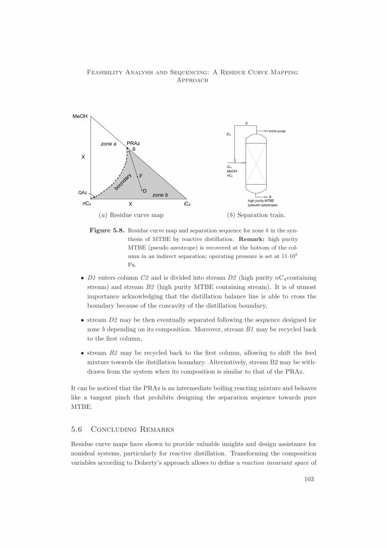
Feasibility Analysis and Sequencing: A Residue Curve MappingApproach
boun
dary F
D
MeOH
zone b
zone a PRAz
QAz
B
X
X
(a) Residue curve map
high purity MTBE�(p�seudo azeo�trope)�
inert�s purge�
D
B
(b) Separation train.
Figure 5.8. Residue curve map and separation sequence for zone b in the syn-
thesis of MTBE by reactive distillation. Remark: high purity
MTBE (pseudo azeotrope) is recovered at the bottom of the col-
umn in an indirect separation; operating pressure is set at 11·105
Pa.
• D1 enters column C2 and is divided into stream D2 (high purity nC4containingstream) and stream B2 (high purity MTBE containing stream). It is of utmostimportance acknowledging that the distillation balance line is able to cross theboundary because of the concavity of the distillation boundary,
• stream D2 may be then eventually separated following the sequence designed forzone b depending on its composition. Moreover, stream B1 may be recycled backto the first column,
• stream B2 may be recycled back to the first column, allowing to shift the feedmixture towards the distillation boundary. Alternatively, stream B2 may be with-drawn from the system when its composition is similar to that of the PRAz.
It can be noticed that the PRAz is an intermediate boiling reacting mixture and behaveslike a tangent pinch that prohibits designing the separation sequence towards pureMTBE.
5.6 Concluding Remarks
Residue curve maps have shown to provide valuable insights and design assistance fornonideal systems, particularly for reactive distillation. Transforming the compositionvariables according to Doherty’s approach allows to define a reaction invariant space of
103

Chapter 5
lower dimension, formed by attainable product compositions and where the conventionalconcepts for residue curves can be applied.
For the MTBE synthesis two main subregions were defined in the modified compositionsimplex, each of both characterized by singular points (nodes and saddles) and de-limited by separation boundaries. Two different separation sequences were generated,covering all the possible reacting mixture compositions. In the generated sequences,high-purity MTBE was obtained as a product, due to the appearance of a pseudo re-active azeotrope, which imposes limitation to the separation task. As all geometricalmethods, the RCM technique is limited by its intrinsic graphical nature and requiresaccurate thermodynamic data to correctly describe reactive distillation processes. Fur-thermore, RCM technique is suitable only for equilibrium-based processes, which arerelatively common in industrial practice (Fien and Liu, 1994).
The combinatorial number of possible separation sequences for multicomponent mix-tures is considerably large and calls for the definition of heuristics and thermodynamicguidelines based on RCMs to find convenient initial designs. Furthermore, operationalissues should be addressed in terms of, for instance, predicting the controllability of thesequence and defining feasible operational parameters (e.g. reflux ratios).
boun
dary
B2F M1
D2
D1
MeOH
zone b
zone a PRAz
QAz
B1
X
X
(a) Residue curve map
B1
to sequence zone b
M1F
D2
D1
B2MeOH
C1 C2
(b) Separation train.
Figure 5.9. Residue curve map and separation sequence for zone a in the
synthesis of MTBE by reactive distillation. Remark: operating
pressure is set at 11·105 Pa; stream D1 may contain all species
and be close to the distillation boundary; stream D2 may be an
inert nC4 - stream; stream B2 may have a composition similar to
the PRAz.
104

Feasibility Analysis and Sequencing: A Residue Curve MappingApproach
Mind journey to the scientific questions.
If we take a mind journey back to the engineering/scientific de-sign question given at the beginning of this chapter, the followingremark can be made. Two design aspects of the multiechelon de-sign approach are considered in this chapter: feasibility analysisand column sequencing. The RCM technique is identified as aneffective easy-to-use tool to assist the designer in those tasks, par-ticularly for the case of reactive feeds outside conventional com-position ranges. Regarding Question 6, a new (at least morerefined) tool is developed to assist the design of RD processes.
105


“If people never did silly things, nothing intelligent would ever
get done.”
Ludwig Wittgenstein, philosopher (1889-1951)
6Spatial and Control Structure Design in
Reactive Distillation †
In this chapter the fifth space (internal spatial structure) of the multiechelon approach
(cf. chapter 4) in RD design is studied. This design space is addressed from two
perspectives. In the first section, a multilevel modeling approach is proposed as a
tool for the decision-making task in the design of spatial structures of RD processes.
The proposed strategy involves formulating the simulation problem at different levels
of increasing degree of complexity, in which mass, energy and momentum balances are
conveniently applied to represent the behavior of the process. In the second section
of this chapter, the interactions between spatial and control design are discussed.
Both spatial-related and control-related design variables are optimized with respect
to economic and dynamic performance in the presence of time-varying disturbances.
The synthesis of MTBE is used as tutorial example in the course of this chapter.
†Parts of this chapter have appeared in Almeida-Rivera et al. (2003)
107

Chapter 6
6.1 Multilevel Modeling
6.1.1 Introduction
As already discussed in previous chapters, model development and design methodologiesof RD processes are far more complex than those involved in conventional reactors andseparation technologies. Therefore, novel and systematic approaches are required tosupport the decision-making tasks for planning, design and operation of this integratedprocess. In this section an approach is suggested as a decision-making tool in theconceptual design of RD processes. This approach allows the designer to obtain firstestimates of the spatial design variables at an external level or envelop and subsequentlydetermine their real values at an internal level using more sophisticated and detailedmodels.
6.1.1.1 Input-Output Information Flow
This space of the multiechelon approach (cf. section §4.5) involves the flow of informa-tion listed in table 6.1. This information is related basically to the unit and internalssizing. Moreover, operational parameters such as reflux ratio and heat duty are consid-ered. It is worth mentioning that although a staged-column configuration is consideredin this subsection, the approach is not restricted to stages geometries. Figure 6.1 de-picts a generic design structure for a RD column configuration. It is composed ofseveral building blocks: condenser, reflux drum, reboiler and (non-) reactive compart-ments. The compartments allow mass and heat flows to enter and leave the unit atany location. A detailed description of the compartments’ characteristics is coveredin chapter 8. All building blocks are connected according to generic rules detailed inchapter 8.
Table 6.1. Input-output information for the internal spatial structure space.
The multiechelon approach is explained in section §4.5.
Design specifications Design/operational variables Domain knowledge
Process: Continuous: - overall balances
- type of task - column diameter - component balances
- number of columns - heat exchange/contacting areas - dynamic behavior
- columns connectivity - catalyst concentration
- feed ratio of reactants - reboil and reflux ratios
- controllers’ parameters
Discrete:
- feed staging
- reactive and nonreactive stages
- withdrawal staging
- control configuration
108

Spatial and Control Structure Design in Reactive Distillation
For this spatial configuration the multilevel approach involves the derivation of twolevels of different complexity and degree of aggregation. These levels are characterizedby inherent assumptions, particular constraints and modeling objectives. All thesefeatures are derived from mass, energy and momentum balances and thermodynamicconstitutive expressions.
The outer input-output level (steady-state) and inner task level (dynamic) are conve-niently linked by the extent of reaction (ε), which allows one to establish whether or notthe business-related decision variables cope with the constraints imposed by the problemformulation. Moreover, from this approach it can be elucidated whether or not the cor-responding models are well specified and mutually consistent. A successful realizationat the outer level (column-level) would suggest relaxing constraining assumptions andstepping up to the more rigorous modeling framework (task-level). Furthermore, thisapproach allows the designer to determine whether or not the business-related decisionvariables cope with the operational constraints imposed by the problem formulation.
Recalling the engineering and scientific design questions given in chapter 1, in thischapter we address question 6, namely,
• What (new) methods and tools are needed for reactive distillation process synthesis,analysis and evaluation?
6.1.2 Level 1: Input-Output Level
The envelop defined at this level of aggregation is delimited by the overall superstructure(see figure 6.1). The streams of mass and heat are given by: (i) the feed streams enteringthe structure; (ii) the product and side streams leaving the structure; and (iii) all heattransferred to the structure.
At this input-output level the following assumptions are considered: (i) steady-statemodeling; (ii) multiple feeds (nfeed ∈ Z+), side draw-off streams (noff ∈ Z+), heatstreams (nq ∈ Z+), reactions (nrx ∈ Z+) and components (nc ∈ Z+); and (iii) singlebottom and distillate streams. Component and energy balances are performed over thestructure. The component molar balances (MC) include the distillate, bottom, feedand draw-off streams and the production (or consumption) of species due to chemicalreaction,
MCi =j=nfeed∑
j=1
F feedj × zfeed
j + VTi × ε+ · · · (6.1)
· · · −D× xDi −B× xB
i −k=noff∑
k=1
F sidek × pk = 0, i ∈ Z
nc ,
109

Chapter 6
2
n-1
B
D
Qcond
Qreb
1
n
Ffeed2
Ffeed33
n-3
n-2Ffeedn-2
Ffeedn-1
Fside2
Fside3
Fsiden-3
Fsiden-2
Q2
Q3
Qn-3
Qn-2
input-output level
task level
Figure 6.1. Schematic representation of the overall design structure for a RD
structure. Nomenclature: F feed: feed flowrate; B : bottom
flowrate; D : distillate flowrate; F side: side stream; Q : heat duty.
Remarks: mass and heat flows are allowed to enter and/or leave
the unit at any point; compartments are numbered from top to
bottom; dashed lines define the envelopes for input-output and
task levels.
where F feed, B, D, F side are the molar rates of feed, bottom, distillate and side draw-off streams, respectively; zfeed, xD, xB , p are the molar fractions vector for the feed,distillate, bottom and side draw-off streams, respectively; Vi is the vector (nrx × 1) ofstoichiometric factors of component i in the nrx reactions and ε is the vector (nrx × 1)of the overall extents of reaction.
The overall energy balance (E) is given by the heat requirements of the reboiler and con-denser, heat of reaction, draw-off heat duties and the enthalpy of all involved streams.Thus,
E =i=nfeed∑
i=1
F feedi × (hfeed
i ) + (−∆rH)T × ε−B× hB + · · · (6.2)
· · · −D× hD −j=noff∑j=1
F sidej × hP
j +i=nq∑k=1
Qk −Qcond +Qreb = 0,
110

Spatial and Control Structure Design in Reactive Distillation
where h is the molar enthalpy without heat of formation, Qcond is the condenser duty,Qreb is the reboiler duty, Qk is the draw-off heat rate at stage k and ∆rH is the rowvector of heats of chemical reaction.
Normalization expressions for molar fractions are additionally included in the problemformulation. The set of balance expressions 6.1 and 6.2 turns to be well-posed by spec-ifying appropriate decision variables according to a degree of freedom analysis. Thus,for a given set [nc, nfeed, nq, noff,∆Hrx,V ] and an extent of reaction ε, the modelingproblem is consolidated by removing the degrees of freedom, grouped in vector A,
A =
(nc − 1)(nfeed)zfeed (nc − 1)(noff)p (nc − 1)xD (nfeed)TF
(noff)TP TD (nq)Q Qreb
Qcond (nfeed)Ffeed (noff)Fside B
. (6.3)
Special attention should be paid in the definition of A. The specification of its variablesshould take into account the physical feasibility of the problem solution. Thus, vectorA includes variables such as compositions of all incoming streams, compositions of alloutgoing streams (side, distillate and bottom streams), temperatures of all incomingand outgoing streams, heat duties of reboiler and condenser, heat flows transferred toeach compartment and the molar flows of all feed streams, side streams and bottomstream.
The column-level simulation problem is then stated as follows,
Given : ε and A,
Solve for : Xvariables,
s.t. : |YtotalX
| = 0,Ffeed, D,B,Fside ∈ R+,
Qreb, Qcond,Q ∈ R,
zfeed,xD,xB,p,∈ [0, 1],
(6.4)
where Xvariables is the set of all involved variables (2(nfeed +noff)+nc(nfeed +noff +2)+6+nq), Ytotal is the set of algebraic equations obtained from mass (expression 6.1) andenergy balances (expression 6.2) and normalization expressions (nc + nfeed + noff + 3).
Relevant information is extracted from this level with respect to process flow/blockdiagram possibilities and estimation of boundary conditions. The practical gain ofthis approach is the assessment of the effect of the extent of reaction vector on theproduct stream(s). More specifically, at a given set of input design variables, flowand composition might be computed having the extent of reaction vector as an inputparameter. Moreover, the output of this aggregation level defines good design targetsfor the task-oriented level.
111

Chapter 6
Q
F feed,Vn
Rx
F Vn+1
F side,Vn
F Vn
F feed,Ln
F Ln
F Ln-1
F side,Ln
Figure 6.2. Schematic representation of the generic lumped reactive distil-
lation volume element (GLRDVE). Nomenclature: Ffeed,(α)i :
feed flowrate of phase (α) at position i ; Fside,(α)i : flowrate of side
stream corresponding to phase (α) at position i ; Ψm: interfacial
mass transfer flux; Ψe: interfacial energy transfer flux; Q : heat
duty.
6.1.3 Level 2: Task-Level
At this modeling level the internal working of the column is taken into account (i.e. reac-tion rates, mass and heat transfer). A generic lumped RD volume element (GLRDVE)is conceived to represent any element within the RD column along with its occurringtasks and around the steady-state defined in level 1. As depicted in figure 6.2 theGLRDVE allows one to account for the presence of incoming and outgoing streams(feeds/draw-offs), the change of chemical identity and the removal/addition of heat.The novelty of this approach stems from the derivation of four independent sub-moduleswithin the GLRDVE. Those sub-modules are characterized by the dynamic behaviorof unique tasks: reaction/separation, separation without reaction, mixing and heatexchange module. A detailed derivation of the first principles occurring within theGLRDVE is addressed in section §8.2.
Along the same line of reasoning Papalexandri and Pistikopoulos (1996) present a gen-eralized modular approach for process synthesis, which includes among other reactive-separation building blocks. Relevant is the definition of thermodynamic-based connec-tivity rules among the different blocks and the optimization-driven approach used. Re-cent contributions by Proios and Pistikopoulos (2005) extend the work of Papalexandriwith a particular focus on separation trains. All dynamic sub-models imply character-istic assumptions and the presence of species mass and energy balances in the volumeelement and the inclusion of hydraulic, constitutive and normalization expressions. In
112

Spatial and Control Structure Design in Reactive Distillation
general terms, the key sets of equations include: (i) conservation equation of speciesmass, energy and electrical charge; (ii) phase and reaction equilibrium equations; (iii)thermodynamic constitutive equation per phase, involving density, specific heat andfugacity coefficients; (iv) approximations to the momentum balance involving pressuredrop, phase ratio and phase contact area; and (v) kinetic equation for chemical reac-tions, mass and heat transfer between lumped phases.
Thus, for any GLRDVE the set of involved expressions is given with respect to mathe-matical structure by,
Given : f(x(t), x(t), u(t), y(t), z) = 0, t ∈ [t0, tf ],g(x(t), u(t), y(t), z) = 0, t ∈ [t0, tf ],h(x(t), u(t), y(t), z) ≤ 0, t ∈ [t0, tf ],i(x(0), u(0), y(0), z) = 0,
Solve for : x(t) ∈ X ⊆ Rx, u(t) ∈ U ⊆ Ru, y(t) ∈ Y ⊆ Ry, t ∈ [t0, tf ],z ∈ Z ⊆ R
z,
(6.5)
where f (·), g(·) and h(·) are sets of differential, algebraic equality and inequality equa-tions, respectively, i(·) is the set of initial conditions, x is the set of state variables, u isthe set of input variables, y is the set of output variables and z denotes time-invariantparameters.
During the model development for the GLRDVE the following assumptions are made:(i) the liquid and vapor streams leaving a compartment are in thermodynamic equilib-rium; (ii) the liquid and vapor in each compartment are perfectly-well mixed (i.e. noradial gradient in temperature and composition); (iii) the reactions are taking place inthe liquid phase and enhanced by a solid catalyst; (iv) the reactions occur only in thecompartments containing catalyst; and (v) vapor and liquid entrainment is neglected.
The assumed extents of reaction at level 1 (input-output) define the targeted conversionfor the various species. At the inner level (task level) the cumulative effect of all localconversions should match the targets at the outer level, whenever physically feasible.This constraining information might be expressed as follows (Melles et al., 2000),
s.t. : |εinput-output level − εtask level| − εε ≤ 0. (6.6)
Figure 6.3 visualizes the link between both levels and the streams shared by them. Notethat the actual input variables to both levels are given by formulation 6.4.
6.1.4 Case Study: Synthesis of MTBE
The multilevel modeling approach is applied to the synthesis of MTBE at 11·105 Pa in astaged RD column loaded with solid catalyst. A detailed description of the system can
113

Chapter 6
I/O level task level
feed streams: flows, compositions, temperatures
heat duty
outgoing streams: flows,
compositions, temperatures
modules
connectivity
Figure 6.3. Schematic representation of the link between the input-output
level and the task level. Remark: the actual input variables to
the levels are given by the formulation 6.4.
be found in appendix B. The reaction kinetics is estimated according to the pseudo-homogenous expression reported by Mohl et al. (1999); Sundmacher and Hoffmann(1999) and Schrans et al. (1996),
gj(x, T ) =(
aiC4
aMeOH− aMTBE
Keq × a2MeOH
), (6.7)
where g(·) is the chemical reaction driving force based on activities and Keq is thetemperature-dependent chemical equilibrium constant.
The spatial structure of the reactive distillation column is similar to that reported byHauan et al. (1995a) and Jacobs and Krishna (1993) and detailed in the upper sectionof table 6.2.
At the input-output level an initial decision is made according to formulation 6.4. Bot-tom compositions are specified, from which the extent of reaction is computed usinginput-output model. A desired value of 150 mol×s−1 is imposed to the overall extentof reaction and the set Ytotal
Xis successfully solved for a wide range of A values. As
feasible solutions are shown to exist, the decision of solving the simulation problemaccording to the task model formulation 6.5 is made. The task-level model is developedin gPROMS c©/gOPT c©(PSEnterprise, Ltd.) equation-oriented environment. The setof expressions f(·), g(·) and h(·) are simultaneously solved provided an appropriate setof initial conditions i(·). Moreover, the sizing design variables (column diameter andreboiler and condenser areas, listed at the lower section of table 6.2) are convenientlychosen by the algorithm to avoid any violation of the extent of reaction constraint 6.6and hydraulic considerations. As depicted in figure 6.4, the components’ compositionsshow an expected behavior at a simulation time that guarantees steady-state condition.A highly pure MTBE stream is drawn at the bottom of the unit; whereas the top stream
114

Spatial and Control Structure Design in Reactive Distillation
Table 6.2. Nominal values in the MTBE synthesis. Remark: operational
conditions are those reported in Hauan et al. (1995a); Jacobs and
Krishna (1993); Seader and Henley (1998).
Value
Number of trays 15 [2:rectifying;8:reactive; 5:stripping]
Feed 1: location iC4+ nC4 : 10th tray (g)Feed 1: flowrate 455 mol×s−1
Feed 1: composition iC4 : 0.37; nC4 : 0.63Feed 1: temperature 350KFeed 2: location MeOH: 9th tray (l)Feed 2: flowrate 168 mol×s−1
Feed 2: composition MeOH: 1.00Feed 2: temperature 320KOperating pressure 11·105 Pa (top)Reflux ratio 7Mass of catalyst/tray 204.1 kg=1000 eq[H+]
Extent of reaction 150 mol×s−1
Column diameter 3.573 mCondenser area 4.460·101 m2
Reboiler area 2.456·102 m2
is predominantly composed of inert nC4 . Furthermore, the problem formulations 6.5,6.4 and 6.6 are solved without violating any constraint at both levels of detail.
6.2 Simultaneous Optimization of Spatial and Control Struc-
tures in Reactive Distillation
The interactions between spatial and control design have been classical subjects of aca-demic research during the last decade. It is widely accepted -in both academia andindustry- that controllability and operability issues play an essential role in the designof chemical processes. The traditionally-used sequential approach (i.e. spatial designfollowed by control structure design) leads frequently to units/process with poor control-lability and responsiveness properties and inoperative in the presence of disturbancesand/or uncertainties in design parameters. Relevant developments in this field havebeen reported (e.g. Skogestad and Postlethwaite (1999) and recently by Meeuse andTousain (2002)) with the aim to consider operability and controllability aspects in theearly stage of the design cycle. However, most of such contributions rely on linearizationtechniques around operational points, steady state models or nonapplicable/complicatecontrollability indices.
115

Chapter 6
2 4 6 8 10 12 14 16
0.1
0.2
0.3
0.4
0.5
0.6
0.7
0.8
0.9
Tray location [−]
Molar fraction [−]
CH3OH
iC4
MTBE
Figure 6.4. Composition profiles in the synthesis of MTBE obtained by a
multilevel modeling approach. Remarks: the molar fraction
of nC4 is not plotted; a target value of 150 mol×s−1 is imposed
to the overall extent of reaction; the spatial configuration of the
unit is given in table 6.2; time horizon is 14400 s.
This section addresses the application of a dynamic optimization-based design approachto RD. The liquid-phase esterification reaction of iC4 and methanol in the presence ofinert nC4 in a staged RD column is used as tutorial example. Similar to the studyon binary distillation (Bansal et al., 2000; Bansal, 2000) and on the synthesis of ethylacetate by RD (Georgiadis et al., 2002), both spatial-related (e.g. column diameterand heat exchanger areas) and control-related (e.g. gain, set-point and reset time)design variables are optimized with respect to economic and dynamic performance inthe presence of time-varying disturbances.
6.2.1 Description of the Design and Control Problem in Reactive Distil-
lation
Generally speaking, a chemical process that shows poor ability of meeting control ob-jectives gives rise to missing opportunities with respect to economic performance andsatisfaction of product specifications. This fact may imply the existence of a trade-offbetween those processes designed with respect to control performance considerations
116

Spatial and Control Structure Design in Reactive Distillation
and those driven by economic issues. In order to circumvent this inconvenient duality,a novel design approach has been proposed (Bansal et al., 2000; Bansal, 2000; Geor-giadis et al., 2002) where both economic and control oriented issues are convenientlyincorporated in the formulation of the optimization problem and simultaneously solved.
In the case of RD design, the general design and control problem involves finding pa-rameters (continuous and/or integers), which define the RD column and control tuningparameters at the minimum economic cost and with an acceptable dynamic performancein the presence of disturbances. The continuous parameters include column diameter,reboiler and condenser areas and tuning parameters (gain Kc, set-point SP and resettime τc), while integer variables involve the existence or not of catalyst on a given stage(y = 1 for reactive stage and y = 0 for nonreactive stage). Alternatively, the presenceof catalyst on a tray can be expressed using the Kronecker delta function. For the sakeof comparison with literature data, the amount of catalyst is assumed to be identicalon all reactive trays.
6.2.2 Description of the Dynamic Optimization Problem in Reactive Dis-
tillation
All involved expressions are combined in the formulation of an optimization problem.The set of expressions includes: (i) conservation equation of species mass, energy andelectrical charge; (ii) phase and reaction equilibrium equations; (iii) thermodynamicconstitutive equation per phase, involving density, specific heat and fugacity coeffi-cients; (iv) approximations to the momentum balance involving pressure drop, phaseratio and phase contact area; and (v) kinetic equation for chemical reactions, mass andheat transfer between lumped phases. Additionally, algebraic expressions are includedto account for constitutive relations and to estimate physical properties of the compo-nents, plate hydraulics, column sizing and economic performance indices. A detaileddescription of the model can be found in appendix A. Thus, the general optimizationproblem is formulated as follows (Bansal et al., 2000; Bansal, 2000),
Obj. : minzp,zc,y
tf∫0
J(xd(tf ), xa(tf ), u(tf ), d(tf ), y(tf ), pp(tf ), pc(tf ), zp, zc, y, tf )dt,
s.t. : f(x(t), x(t), u(t), d(t), y(t), pp(t), pc(t), zp, zc, y) = 0, t ∈ [t0, tf ],g(x(t), u(t), d(t), y(t), pp(t), pc(t), zp, zc, y) = 0, t ∈ [t0, tf ],h(x(t), u(t), d(t), y(t), pp(t), pc(t), zp, zc, y) ≤ 0, t ∈ [t0, tf ],i(x(0), u(0), d(0), y(0), pp(0), pc(0), zp, zc, y) ≤ 0, t ∈ [t0, tf ],x(t) ∈ X ⊆ Rx, u(t) ∈ U ⊆ Ru, d(t) ∈ D ⊆ Rd, y(t) ∈ Y ⊆ Ry, t ∈ [t0, tf ],zp ∈ Zp ⊆ Rzp
, zc ∈ Zc ⊆ Rzc
,
pp(t) ∈ P p ⊆ Rpp
, pc(t) ∈ P c ⊆ Rpc
, t ∈ [t0, tf ],y ∈ [0, 1],
(6.8)
117
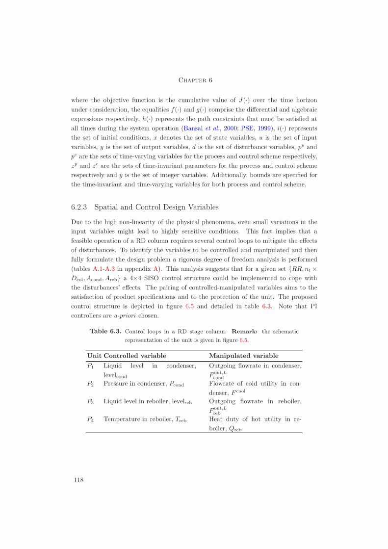
Chapter 6
where the objective function is the cumulative value of J (·) over the time horizonunder consideration, the equalities f(·) and g(·) comprise the differential and algebraicexpressions respectively, h(·) represents the path constraints that must be satisfied atall times during the system operation (Bansal et al., 2000; PSE, 1999), i(·) representsthe set of initial conditions, x denotes the set of state variables, u is the set of inputvariables, y is the set of output variables, d is the set of disturbance variables, pp andpc are the sets of time-varying variables for the process and control scheme respectively,zp and zc are the sets of time-invariant parameters for the process and control schemerespectively and y is the set of integer variables. Additionally, bounds are specified forthe time-invariant and time-varying variables for both process and control scheme.
6.2.3 Spatial and Control Design Variables
Due to the high non-linearity of the physical phenomena, even small variations in theinput variables might lead to highly sensitive conditions. This fact implies that afeasible operation of a RD column requires several control loops to mitigate the effectsof disturbances. To identify the variables to be controlled and manipulated and thenfully formulate the design problem a rigorous degree of freedom analysis is performed(tables A.1-A.3 in appendix A). This analysis suggests that for a given set {RR, nt ×Dcol, Acond, Areb} a 4×4 SISO control structure could be implemented to cope withthe disturbances’ effects. The pairing of controlled-manipulated variables aims to thesatisfaction of product specifications and to the protection of the unit. The proposedcontrol structure is depicted in figure 6.5 and detailed in table 6.3. Note that PIcontrollers are a-priori chosen.
Table 6.3. Control loops in a RD stage column. Remark: the schematic
representation of the unit is given in figure 6.5.
Unit Controlled variable Manipulated variable
P1 Liquid level in condenser,levelcond
Outgoing flowrate in condenser,F out,L
cond
P2 Pressure in condenser, Pcond Flowrate of cold utility in con-denser, F cool
P3 Liquid level in reboiler, levelreb Outgoing flowrate in reboiler,F out,L
reb
P4 Temperature in reboiler, Treb Heat duty of hot utility in re-boiler, Qreb
118

Spatial and Control Structure Design in Reactive Distillation
1
15
9
10
MeOH
C4-stream
3
MTBE(>99%m)
MTBE(<0.1%m)
reactivezone
P
L
L
T
Fcool
Pcond
levelcond
levelreb
Treb
Qreb
Fout,Lcond
Fout,Lreb
FR,L FD,L
Figure 6.5. Control structure in the synthesis of MTBE by RD. Remark:
the manipulated and controlled variables for each control loop
are listed in table 6.3.
6.2.3.1 Case Study: Synthesis of MTBE
A detailed description of this system is available in appendix B. The spatial structureof the RDC is similar to that reported by Hauan et al. (1995a) and Jacobs and Krishna(1993) and detailed in the upper section of table 6.2. Two sinusoidal disturbances (figure6.6) are included in the problem description. They account for both the variation in thefeed composition of the C4-stream and the change in the inlet temperature of the coldutility T in,cool during the process operation. As suggested by Georgiadis et al. (2002);Bansal et al. (2000), the feed composition disturbance is modelled as a fast movingfunction and represented by the following general expression,
zfeed =
zfeed
iC4 ,0 + σf (t)zfeed
MeOH,0
zfeednC4 ,0 − σf (t)zfeed
MTBE,0
, with σf (t) := 0.05× sin(
2× π
3600× t). (6.9)
The composition disturbance frequency mimic an upstream time response of 1 hour,which is commonly occurring in industrial practice.
The temperature disturbance tries to represent the variation of inlet temperature of the
119

Chapter 6
0 2000 4000 6000 8000 10000 12000 14000
0.35
0.40
0.45
0.50
0.55
0.60
0.65
Molar fraction [-]nC
4
iC4
Time [s]
(a) Fast moving disturbance in the feedcompositions of iC4 and nC4 , zfeed.
0 2000 4000 6000 8000 10000 12000 14000282
284
286
288
290
292
294Tin,cool [K]
Time [s]
(b) Slow disturbance in the inlettemperature of the cold utility, T in,cool.
Figure 6.6. Time dependence of the disturbances scenario in the dynamic
optimization of MTBE synthesis by reactive distillation. Time
horizon=14400 s.
cooling medium during the time horizon. Thus,
T in,cool = 298 + σs(t), with σs(t) := 5× sin(2× π
14400× t). (6.10)
In this case, the temperature disturbance has a time response of 4 hours.
6.2.3.2 Nominal Spatial/Control Design
Nominal design values of the spatial structure of the column for the synthesis of MTBE(i.e. column diameter and reboiler and condenser heat exchange areas) are firstly es-timated. They are obtained by solving a steady-state optimization problem, whichminimizes the total annualized cost of the RD unit in the absence of disturbances. Thefollowing constraints are included to the problem formulation: (i) the column diameteris bounded by flooding conditions; (ii) the heat exchange areas of the condenser andreboiler are estimated by bounded values of outlet temperatures of the hot and coldutilities, and (iii) the molar fraction of MTBE at the top and bottom stream is con-strained to values lower than 0.1% and 99% respectively. Thus, the statics optimizationproblem results in,
120

Spatial and Control Structure Design in Reactive Distillation
Function: minDcol,Areb,Acond
J = TAC,
s.t. : g(·) = 0,h(·) ≤ 0,Dmin
col ≤ Dcol ≤ Dmaxcol ,
Aminreb ≤ Areb ≤ Amax
reb ,
Amincond ≤ Acond ≤ Amax
cond,
xDMTBE ≤ 0.1% and xB
MTBE ≥ 99%,
(6.11)
where TAC is the total annualized cost of the RD unit and includes operational andinvestment costs. A detailed specification of the terms involved in the definition of TACis presented in the appendix A.1.
The relevant results of the optimized steady-state nominal design together with thenominal design inputs are presented in table 6.4. According to the sequential approach,the control structure is chosen and controllers’ parameters are estimated only afterthe spatial structure is known and a disturbance scenario is defined. For the sake ofsimplicity and according to the degree of freedom analysis in appendix A, the controlstructure depicted in figure 6.5 is implemented in the RD unit.
Table 6.4. Optimized steady-state design of a RD column for MTBE syn-
thesis. The parameter ∆xMTBE accounts for the error between
computed and set-point values for the molar fractions of MTBE in
the top and bottom streams.
Value
Number of trays 15 [2:rectifying;8:reactive; 5:stripping]
Feed 1: location iC4+ nC4 : 10th tray (g)Feed 1: flowrate 455 mol×s−1
Feed 1: composition iC4 : 0.37; nC4 : 0.63Feed 1: temperature 350KFeed 2: location MeOH: 9th tray (l)Feed 2: flowrate 168 mol×s−1
Feed 2: composition MeOH: 1.00Feed 2: temperature 320KOperating pressure 11·105 Pa (top)Reflux ratio 7Mass of catalyst/tray 204.1 kg=1000 eq[H+]
Bottom flowrate 197 mol×s−1
∆xMTBE 2.2 ·10−5
Column diameter 7.132 mCondenser area 1.059·103 m2
Reboiler area 6.93·102 m2
121

Chapter 6
Tuning the controllers is initially carried out based on engineering judgement in com-bination with the rules of thumb given by Luyben (2002). Hence biases are set to thecorresponding steady state values, gains are such that a variation of approximately 50%of the controlled-variable value is achieved by a change of 1% in the value of the ma-nipulated variable and reset times are set around 1-2 minutes. To better estimate thevalues of the controllers gains a sensitivity analysis is performed considering a simplifieddisturbance scenario given by the variation (+10%) of the flowrate of methanol. For thesake of exemplification, figures 6.7a-d depict the dynamic behavior of the controllers’input variables in this simplified disturbance scenario. It can be noticed that an ac-ceptable dynamic behavior of the different condenser and reboiler blocks is obtained(see bold curves in figures 6.7a-d). For practical purposes these controllers parame-ters are considered only as initial guesses for the optimization formulation addressedlater on. The problem of estimating the controllers’ parameters is now formulated asan optimization problem in the time domain, aiming at a minimization of the integralabsolute error of the control loops. This criteria is in particular chosen for the sake ofcomparison with the work of Georgiadis et al. (2002).
The two sinusoidal disturbances introduced previously (expressions 6.9 and 6.10) areincluded in the optimization problem, resulting in the generic formulation,
Function: minKi,Biasi,τc,i,SPi
J =tf∫0
[(xb − xb)2 + (xd − xd)2
]dt,
s.t.: f(·) = 0 t ∈ [t0, tf ],g(·) = 0 t ∈ [t0, tf ],h(·) ≤ 0 t ∈ [t0, tf ],d(·) = 0 t ∈ [t0, tf ],Tmin
reb ≤ Treb ≤ Tmaxreb t ∈ [t0, tf ],
T out,minwater ≤ T out
water ≤ T out,maxwater t ∈ [t0, tf ],
T out,minsteam ≤ T out
steam ≤ T out,maxsteam t ∈ [t0, tf ],
(6.12)
where the objective function J accounts for deviations from product and top specifica-tions (x), the constraint paths set bounds for the temperature in the reboiler and theoutlet temperatures of the cold and hot utilities and the set of disturbances (Equations6.9 and 6.10) are grouped in the vector d(·).Solving problem 6.12 leads to the set of controllers’ parameters listed in the secondcolumn of table 6.5.
6.2.3.3 Simultaneous Optimization of Spatial and Control Structures
In this subsection the sequential approach adopted previously is effectively replacedby a formulation in which both spatial and control-related constraints are included inthe optimization problem and solved for the most economic operation. Besides the
122

Spatial and Control Structure Design in Reactive Distillation
already mentioned constraint paths, the following spatial-related constraints have beenincluded,
0 10000 20000 30000 40000 50000 60000
0.498
0.499
0.500
0.501
0.502
0.503
K=-1000
K=-100
lcond
[m]
Time [s]
(a) Level in the condenser
0 10000 20000 30000 40000 50000 60000
11.096
11.098
11.100
11.102
11.104
11.106
Pcond
[bar]
K=-2.0 10 5
K=-2.0 10 4
Time [s]
(b) Pressure in the condenser
0 10000 20000 30000 40000 50000 60000
0.2
0.3
0.4
0.5
0.6
0.7
0.8
lreb
[m]
K=-100
K=-10
Time [s]
(c) Level in the reboiler
0 10000 20000 30000 40000 50000 60000428.0
428.1
428.2
428.3
428.4
428.5
428.6
428.7
428.8
428.9
429.0
429.1
429.2
K=4.0 10 4
K=4.0 10 5
Treb
[K]
K=4.0 10 6
Time [s]
(d) Temperature in the reboiler
Figure 6.7. Dynamic behavior of the controllers’ input (controlled) variables
in the synthesis of MTBE. Remarks: the disturbance scenario
involves the time dependent variation of the flowrate of methanol:
FMeOH = F SSMeOH + δ(t)FMeOH , with δ(t)FMeOH = 0.1 × F SS
MeOH
if 10000s < t < 40000s and δ(t)FMeOH = 0 if 10000s > t or
t > 40000s; controllers parameters are only considered as initial
estimates.
123

Chapter 6
Function: minKi,Biasi,τc,i,SPi,Dcol,Areb,Acond
J =tf∫0
[TAC]dt
s.t.: f(·) = 0 t ∈ [t0, tf ]g(·) = 0 t ∈ [t0, tf ]h(·) ≤ 0 t ∈ [t0, tf ]d(·) = 0 t ∈ [t0, tf ]Tmin
reb ≤ Treb ≤ Tmaxreb t ∈ [t0, tf ]
T out,mincool ≤ T out
cool ≤ T out,maxcool t ∈ [t0, tf ]
T out,minheat ≤ T out
heat ≤ T out,maxheat t ∈ [t0, tf ]
Dmincol ≤ Dcol ≤ Dmax
col
Aminreb ≤ Areb ≤ Amax
reb
Amincond ≤ Acond ≤ Amax
cond
(6.13)
The optimized parameters of problem 6.13 are listed in the third column of table 6.5.By comparing the TAC of both approaches, it can easily been inferred that the si-multaneous optimization of both spatial and control structures leads to a cheaper andmore controllable process than that obtained via the conventional sequential strategy.Although the relative difference between both economic indexes is fairly small, the ac-cumulative cost saving sums up to 0.2 million euros per year. This cost reduction ispredominantly originated from the reduced column diameter and smaller reboiler.
The time evolution of the product compositions and temperature profile at the end-point are depicted in figure 6.8 for the simultaneous approach. It should be noticedthat the variations of MTBE composition are negligible from a practical stand-point.Moreover, the temperature along the unit presents a steep increase only at the strippingsection. Heat effects due to exothermicity are relatively mild.
6.3 Concluding Remarks
The conclusions derived from this chapter are grouped in accordance to the above-mentioned sections. Firstly, it is worth mentioning that the approach presented in thischapter has been applied to staged units, without it being restricted to that geometry.Moreover, variables pairing for the control configuration has not been considered. AMINLP approach could be used to address this last issue, as applied by Bansal et al.(2000, 2003) for binary ideal distillation.
Multilevel modeling. The proposed multilevel modeling approach is able to providean easy-to-handle tool in the early stages of design. Two model levels of different degreeof complexity were derived to model the processes taking place in a RD column. Rigor-ous and reliable degree of freedom analysis were performed at each level, where appro-priate business-related decision variables were included. The outer (input-output) and
124

Spatial and Control Structure Design in Reactive Distillation
Table 6.5. Simulation results for the conventionally-used sequential and si-
multaneous approaches. Remarks: inputs of the design problem
are given in table 6.4; the notation used in the control loops cor-
responds to the description of table 6.3 and figure 6.5; the conver-
gence tolerance of the design variables is 1 ·10−8; catalyst hold-up
is considered constant (relaxation of this assumption is addressed
in chapter 8).
Variable Unit Sequential Simultaneous
P1 K1 - −1.000× 10³ −4.999× 10²
Bias mol×s−1 2.556× 10³ 2.556× 10³
τc s 1.000× 100 5.047× 10⁻¹
SP m 5.000× 10⁻¹ 5.000× 10⁻¹
P2 K2 - −2.000× 10⁴ −9.999× 10⁴
Bias mol×s−1 4.973× 10⁴ 4.973× 10⁴
τc s 1.200× 10² 5.000× 10⁻¹
SP bar 1.100× 101 1.100× 101
P3 K3 - −5.000× 100 −2.500× 101
Bias mol×s 1.517× 10² 1.517× 10²
τc s 1.200× 10² 1.500× 101
SP m 5.000× 10⁻¹ 5.000× 10⁻¹
P4 K4 - 4.000× 10⁵ 2.000× 10⁶
Bias J×s 4.350× 10⁷ 4.350× 10⁷
τc s 1.000× 10² 4.761× 100
SP K 4.289× 10² 4.289× 10²
Dcol m 7.132× 100 6.924× 100
Acond m2 1.059× 10³ 1.250× 10³
Areb m2 6.933× 10² 4.500× 10²
Ctotal euro/y 2.112× 10⁸ 2.108× 10⁸
inner (task) levels were linked by the extent of reaction vector, which allows establishingwhether or not the models are well specified and mutually consistent. Additionally, theapproach allows one to determine whether or not the business-related decision variablescope with the operational constraints imposed by the problem formulation (e.g. SHEissues, reactants availability and market demand).
Simultaneous dynamic optimization. In order to validate this approach, the syn-thesis of MTBE is used as case study. Three spatial variables and sixteen control-relatedparameters were optimized during a time horizon of 14400 s. A tradeoff between controland economic performances exists in the design of RD processes, as shown in table 6.5.The design optimized sequentially with respect to dynamic behavior led to a RD process
125

Chapter 6
0 2000 4000 6000 8000 10000 12000 140000.00000
0.00005
0.00010
0.00015
0.00020
0.00025
0.9975
0.9980
0.9985
0.9990
0.9995
1.0000
top stream
bottom stream
xMTBE
[-]
Time [s]
(a) Molar fraction of MTBE. Timehorizon: 14400 s.
2 4 6 8 10 12 14 16
350
360
370
380
390
400
410
420
430
T [K]
Tray location [-]
(b) Temperature profile along the RDcolumn.
Figure 6.8. Time evolution of MTBE molar fraction in the top and bottom
streams (left) and temperature profiles at the end-point (right) for
the simultaneous optimization of spatial and control structures.
Remarks: the trays are numbered from top to bottom (1st: con-
denser; 17th : reboiler); the sizing and control parameters are
listed in table 6.5.
with a total annualized cost higher than that obtained using simultaneous optimizationof spatial and control structures. This multiobjective optimization problem was solvedby incorporating appropriate time-invariant parameters (e.g. column diameter, heattransfer areas and controllers’ parameters), in the frame of a dynamic optimizationin the presence of deterministic disturbances. A rigorous degree of freedom analysiswas performed to the involved building blocks and an adequate control structure wasimplemented.
Mind journey to the scientific questions.
If we take a mind journey back to the engineering/scientific de-sign question given at the beginning of this chapter, the followingremark can be made. The complexities of RD process design arehandled in this chapter by the definition of an easy-to-handle toolto assist the modeling task. Furthermore, a more design advancedapproach is addressed, which involves the simultaneous dynamicoptimization of spatial and control structures in the presence ofa disturbance scenario. Therefore, the material presented in thischapter contributes to the answering of Question 6.
126

“Engineering is the art or science of making practical.”
Samuel C. Florman, writer and engineer
7Steady and Dynamic Behavior Analysis†
The steady-state and dynamic behavior in RD are studied in line with the proposed
design procedure. Two levels of aggregation are considered: a single stage reactive
flash and a full column. The first configuration is used to address the steady-state
behavior, whereas the full column is used as case study for the process dynamics. By
selecting a reactive flash we focus exclusively on the phenomena interaction rather
than on equipment effects. In this regard, twenty-five bifurcation diagrams are pre-
sented, exhibiting a maximum of three steady states and five feasibility boundaries.
Singularity theory is used to divide the parametric space into regions with quali-
tatively different behavior. Furthermore, parametric dependence of MSS regions is
studied. Additionally, the dynamic behavior of a complete MTBE RD column is cov-
ered. Two deterministic disturbances are included to analyze the unit dynamics. The
control structure is a conventional SISO and PID based one, aiming at disturbance
rejection. This structure is defined based on a combination of rigorous degree of
freedom analysis and engineering judgement. The variations encountered in product
compositions reveal that the unit operates effectively in the presence of disturbances.
The output of this analysis defines the reference case for the new developments to be
introduced in chapter 8.
†Section §7.2.1 on multiplicities in a reactive flash has appeared as Lakerveld et al. (2005).
127

Chapter 7
7.1 Introduction
The sixth design space of the multiechelon approach (cf. chapter 4) in reactive distilla-tion is the focus of this chapter. After having defined the spatial and control structuresthe process behavior in steady-state and dynamic domains are now addressed. Theinput and output information flow at this design space is detailed on table 7.1.
Table 7.1. Input-output information for the behavior analysis space. The
multiechelon approach is explained in section §4.5.
Design specifications Design/operational variables Domain knowledge
Process: Continuous: - steady-state behavior
- unit structure - controllability index - dynamic behavior
- control structure - operating conditions
The analysis of steady-state behavior allows the designer to explore the effect of kinetics,gas/liquid mass transfer and hydrodynamics and the steady-states of the unit. On theother hand, dynamic simulations are carried out to check the robustness of the design,in terms of the ability of maintain product purities and conversion in desired rangewhen disturbances are occurring.
This chapter addresses those two aspects of process behavior: steady-state and dynamicoperation. In the first case, a reactive flash with a rather ideal exothermic isomerizationreaction is considered. This simplified system is selected to account exclusively on theeffect of phenomena interaction on the occurrence of input and output multiplicity.Therefore, any effect related to unit configuration is considered outside the scope of theanalysis.
The second part of this chapter deals with the dynamic behavior of a full RD column,with special focus on the synthesis of MTBE. Although the design of the control struc-ture is rather conventional (SISO and PI controllers), it is regarded as reference casefor the new developments to be introduced in chapter 8.
Recalling the engineering and scientific design questions given in chapter 1, in thischapter we address question 6, namely,
• What (new) methods and tools are needed for reactive distillation process synthesis,analysis and evaluation?
128

Steady and Dynamic Behavioral Analysis
7.2 Steady-State Behavior
7.2.1 Introduction
Section 2.9 has addressed the generalities and sources of steady-state multiplicity inRD processing. Furthermore, special attention has been paid to the implications ofMSS for the design and operation of RD. In this section the steady-state behavior of asimplified RD unit (i.e. reactive flash) is covered for the case of an exothermic isomer-ization reaction with first-order kinetics and light-boiling reactant. Several approachesare employed to analyze the steady-state behavior of a process model. For instance,regions of MSS can be identified by tracing the dependence of the steady state on onevarying parameter (Mohl et al., 1999; Hauan et al., 1995a; Ciric and Miao, 1994; Bauret al., 2001b; Sneesby et al., 1998b,a; Chen et al., 2002). The starting point of ourapproach is provided by the study on MSS in a reactive flash by Rodriguez et al. (2001,2004). They show that multiplicity is caused by the interaction between separationand reaction in systems in which the activation energy and the gradient of boiling tem-perature with composition are sufficiently large. Because VL equilibrium can createmultiple steady states, state multiplicity becomes possible in endothermic or slightlyexothermic systems, which typically do not display multiplicity in a one-phase CSTR.Several examples were considered and parametric studies were performed. In addition,for an isomerization reaction, necessary conditions for multiplicity were derived. Theseconditions are somehow difficult to apply, because they are expressed in terms of systemproperties (e.g. heat of vaporization or heat of reaction), but also include, however, theunknown liquid and vapor phase compositions.
Although Rodriguez’s work is restricted to a single stage flash, it clearly shows that thecombination of reaction and separation is a key cause for multiplicity in RD.
In this section, we approach the reactive flash from a different perspective. We employa dimensionless model and distinguish the state variables (e.g. liquid and vapor com-positions), from system physical parameters (e.g. heat of reaction or activation energy)and control parameters (e.g. feed rate or heat duty). Aiming to uncover the possiblebehavior patterns, we present a considerable number of bifurcation diagrams that arequalitatively different. We demonstrate the importance of the feasibility boundariescorresponding to no-liquid or no-vapor products, illustrated in bifurcation diagrams ex-hibiting three and even five such points. Finally, we show that high heat of reaction,activation energy and reactant volatility enlarge the range of operating parameters forwhich multiple states exist. To the best of our knowledge, such a detailed analysis hasnot been provided yet for the case of RD. Section §7.2.1 is based on the contributionentitled Exothermic isomerization reaction in reactive flash: steady state behavior byLakerveld et al. (2005).
129

Chapter 7
7.2.2 System’s Features and Model Development
The system under consideration intends to be as simplified and ideal as possible, sothat we focus exclusively on the interaction between occurring phenomena. Thus, theproperties of the system include: (i) binary system undergoing a kinetically controlledisomerization reaction A→ B, (ii) the RD flash is operated at isobaric conditions, (iii)the chemical reaction takes place exclusively in the liquid phase and is exothermic, (iv)the reactant A is the lighter component in the system, (v) both phases are assumed tobe well mixed, (vi) gas and liquid phases behave ideally, (vii) vapor holdup is negligiblecompared to the liquid holdup, (viii) vapor pressures are described by Antoine’s correla-tion and (ix ) both components have equal physical properties (i.e. heat of vaporization,heat capacity and density).
TC
Figure 7.1. Schematic representation of a reactive flash for an isomerization
reaction in the liquid phase.
According to the scheme of figure 7.1, pure reactant A is fed to the unit with a flowrate F, pre-heated to temperature T0 and with a vapor fraction ε. The flash is equippedwith a level controller and a pressure controller to maintain the liquid holdup ML andoperating pressure P at desired values. The liquid flow rate L and vapor flow rate V areused as manipulated variables, respectively. Heat is allowed to be added or removed at arate Q in the liquid phase. For the sake of model solvability, a dimensionless model hasbeen derived for the configuration depicted in figure 7.1. The set of governing equationsand physical properties of the system are given in tables 7.2 and 7.3, respectively.The reference values for temperature, flow rate and pressure are: the boiling point ofcomponent A (i.e. Tb,A) and the nominal values of feed flow rate (i.e. Fref) and pressure(i.e. Pref) for an existing design, respectively.
130

Steady and Dynamic Behavioral Analysis
Table 7.2. Set of governing dimensionless expressions for the reactive flash as
depicted in figure 7.1.
Balance Dimensionless expression
Overall mass 0 = l + v − f
Component dxdt = 1
Da (f × z − l × x− v × y) − x× eγ×θ1+θ
BP condition 0 = x× p01 + (1 − x)× p0
2 − p
L-V equilibrium 0 = y× p− x× p01
Energy 0 = f × (θ∗0 − θ) +Da× B× x× eγ×θ1+θ − v× λ+ q
Feed temperature θ∗0 =
θ0 : liquid feed, θ0 < 0
ε× λ : liquid-vapor feed, θ0 = 0
λ+ CpV
Cp × θ0 : vapor feed, θ0 > 0
X ≡
x
l
y
v
θ
, O ≡
Da
f
z
θ∗0p
q
=
k(Tref)× MFref
FFref
zT∗0 −TrefTrefP
PrefQ
Fref×Cp×Tref
, S ≡
γ
B
λ
a1
b1a2
b2
=
Ea
R×Tref−∆rHCp×Tref
∆vHCp×Tref
A1
1A2
A1×B2A2×B1
Remark: the validity of the model is limited by the boundaries v = 0 and l = 0.
Nomenclature: X are unknown variables, O are operation parameters, S are system para-
meters; z, x and y are the molar fractions in the feed, liquid and vapor phases, respec-
tively; f , l and v are the dimensionless feed, liquid and vapor flow rates, respectively
(f = F/Fref, l = L/Fref, v ≡ V/Fref), θ is the dimensionless temperature (θ = T−TrefTref
),
ε is the vapor fraction in the feed (ε ∈ [0, 1]), the component saturation pressure is given
by: p0j = exp(aj1−bj+θ
1+θ), i ∈ Znc , Cp is the heat capacity and the feed temperature is
estimated as,
T ∗0 =
T0 : T0 < Tb,A
Tb,A + ε× ∆vHCp
: T0 = Tb,A
Tb,A + ∆vHCp
+ CpV
Cp× (T0 − Tb,A) : T0 > Tb,A
7.2.3 Classification of Steady States
From the model parameters the dimensionless feed, f, is chosen as distinguished contin-uation parameter and used to depict the dependence of liquid composition, x, for a VLfeed (ε=0.13, T ∗
0 =280K) at different values of dimensionless heat duty, q (figure 7.2).The relevance of the parameter choice is grounded by the fact that feed flow rate de-termines the process throughput and is frequently an operational parameter subjectedto input disturbances (e.g. market demands and supply fluctuations). The parametricspace considered in this study is given by Damkohler number and dimensionless heatduty.
131

Chapter 7
Table 7.3. Properties of the reactive flash system as depicted in figure 7.1.
Remarks: data are taken from Rodriguez et al. (2001, 2004); ac-
cordingly, the reactant is the light-boiling component.
Property Dimensional variable Dimensionless variable
Pre-exponential factor k0=5.88 ·1010 s−1
Antoine coefficients A1 = 9.784 a1 = 9.784A2 = 7.704 a2 = 7.704B1 = 2428 b1 = 1B2 = 2428 b2 = 1.27
Heat of vaporization ∆vH = 4807 kcal×kmol−1
Heat capacity Cp = 20.0 kcal×(kmol×K)−1 λ = 1Heat of reaction ∆rH= 500 kcal×kmol−1 B = 0.1Activation energy Ea= 14454 kcal×kmol−1 γ = 30
Three qualitatively different bifurcation diagrams∗ can be observed if the heat input tothe system is varied. For adiabatic operation (q=0) no feasible solution exists for smallf . As f increases, the number of steady states changes from 0-2-3-1. The lower branchof the curve starts at a feasibility boundary (v=0, marker: �) and exhibits two turningpoints (marker: �), also known as limit or fold . If the heat duty is further increased(q=1), the bifurcation diagram presents the pattern 0-1-3-1. For even larger valuesof q, the bifurcation curves start at the l -boundary (i.e. l = 0 feasibility boundary,marker: •) and a single steady state occurs. It can be noted that the type of diagramdepends on the number and relative location of turning points and feasibility boundaries.These points are normally termed codimension-1 bifurcation or singular points, as theycorrespond to certain values of one single parameter (e.g. f).
Based on the multiplicity behavior of the RD model, a singularity theory approach(Bildea and Dimian, 1999; Gehrke and Marquardt, 1997; Balakotaiah and Luss, 1984)is used to divide the space of model parameters, excluding the distinguished one, intoregions of qualitatively different bifurcation pattern. All nonlinear equations are solvedwith a Newton-Raphson solver routine combined with a local parametrization algorithm(Seydel and Hlavacek, 1987; Razon and Schmitz, 1987; Wayburn and Seader, 1987;Vadapalli and Seader, 2001; Dhooge et al., 2003) to track possible turning points. Todeal with the large number of parameters involved, we adopt the following strategy.First, we achieve the classification in the Da-q space, for a system characterized bysmall heat of reaction, moderate activation energy and high relative volatility. For aVL feed, we identify the main types of behavior occurring in large regions and the
∗The following notation is used for the bifurcation diagrams: BD(p, x; p1, p2), where p denotes the
distinguished parameter, x is the state variable and p1 and p2 are system’s parameters. A BD can be
effectively defined by specifying parameter p1 or p2 in addition to the distinguished parameter p.
132

Steady and Dynamic Behavioral Analysis
10−1
100
101
0
0.1
0.2
0.3
0.4
0.5
0.6
0.7
0.8
0.9
1
f [−]
x [−]
q=0
q=1
q=5
q=2.5
Figure 7.2. Bifurcation diagram f-x at different values of dimensionless heat
duty for a reactive flash undergoing an exothermic isomerization.
Symbols: (�): v = 0 feasibility boundary; (•): l = 0 feasibility
boundary; (�): limit point. Systems features: Da=0.10; z=1;
p=1; θ∗0=0.13; physical properties of the system are listed in table
7.3; governing expressions are given in table 7.2.
important varieties bounding these regions. Afterwards, the effect of the feed conditionθ∗0 , the remaining control parameter, is investigated. Finally, we look at the effect oflarger heat of reaction, larger activation energy and lower relative volatility.
Singularity theory states that the qualitative features of the bifurcation diagram maychange only when the parameter set crosses the hysteresis, isola, or double-limit varieties(Golubitsky and Schaeffer, 1985). Only the hysteresis variety is found to exist for thereactive flash model. When the hysteresis variety is crossed, the number of possiblesteady states changes by two, as two limit points appear or disappear. When feasibilityboundaries exist, the bifurcation diagram may also change at special sets of parameters(Balakotaiah and Luss, 1984). The following varieties are considered in this study,
Variety 1. boundary-limit set (BL): a limit point occurs at a feasibility boundary,
Variety 2. boundary - tangent set (BT ): the bifurcation diagram is tangent to thefeasibility boundary. After crossing this set (e.g. moving from high to lowdimensionless heat duty q in figure 7.5) the bifurcation diagram changesby appearance / disappearance of two feasibility boundaries,
133

Chapter 7
Variety 3. cross-and-limit set (CL): the position of one limit point changes relative toone solution located at the feasibility boundary,
Variety 4. corner set (C ): the bifurcation parameter and the state variable are, simul-taneously, at their boundaries.
Because the defining conditions can be solved for the state variables and two parame-ters (e.g. f and q), the above mentioned varieties are said to be of codimension-2 .The dynamic model of the reactive flash contains several algebraic, but only one differ-ential equation, when the holdup and pressure are fixed and the phase equilibrium isinstantaneous. Such one-dimensional systems cannot exhibit Hopf bifurcations leadingto oscillatory behavior. Therefore, dynamic classification is not necessary.
A better understanding of the steady state classification is carried out by depictingthe loci of codimension-1 singular points in a f -q plot (figure 7.3). As the BD(f, x, q)bifurcation diagrams are obtained for a given value of q, the number and relative locationof singular points can be obtained by the intersection of q=constant (dotted horizontallines in figure 7.3) with the loci of codimension-1 singular points. It can be extractedfrom the figure that at large q, there is only one intersection with the l-boundary,corresponding to the bifurcation diagram I+III in figure 7.4. As q decreases, a narrowregion with three l-boundaries is encountered. This region is bounded by the boundary-tangent points BT1 and BT2 in the q-f plot (zoomed view in figure 7.5a). DiagramII in figure 7.4 represents the behavior in this region. As q is further decreased, twoturning points are met below the cusp H. State multiplicity becomes possible, as shownin diagram IV of figure 7.4. Note that the loci of cusp points is called hysteresis .
Many qualitative changes occur within a small elbow region around q=0, which iszoomed in Figs. 7.5b-d. If we decrease the value of q, the boundary-tangent BT3
is firstly crossed to region V (figure 7.5c) leading to two v- boundaries. Immediately,the relative locations of a turning point and a v-boundary change at a cross-and-limitpoint CL, leading to diagram VI (figure 7.4). By further decreasing q to region VII(figure 7.5b), the v- and l-boundaries move towards f=0 (left section in figure 7.3) anddisappear at a corner point (not shown). One turning point leaves the feasible domainat the boundary limit BL1 and the maximum number of steady states becomes two, asin diagram VIII (figure 7.4). Finally, the turning point left becomes unfeasible and thestate multiplicity disappears as depicted in figure 7.4-diagram XI. Furthermore, a verynarrow range of q values exists (figure 7.5d) where three v-boundaries occur (diagramsIX, X in figure 7.4).
134

Steady and Dynamic Behavioral Analysis
7.2.4 Effect of Damkohler Number, Da
The steady state classification is achieved by tracing the codimension-2 singular pointswhen an additional parameter (e.g. Da) is changed. In this way, the Da-q space isdivided into regions where qualitatively different f -x bifurcation diagrams exist (figure7.6). For each region, the corresponding diagram is presented in figure 7.4. It shouldbe noticed that regions II, V, IX and X, exhibit three feasibility boundaries and arevery small.
7.2.5 Effect of Feed Condition
In the previous section a VL feed (0 < θ∗0 < 1) has been considered. Among thebifurcation diagrams of figure 7.4, those presenting two disconnected branches andthree feasibility boundaries should be remarked. Such diagrams are obtained when BTsets are crossed (see figures 7.5a-d), but are occurring exclusively in narrow regions ofthe Da− q space (figure 7.6). This subsection discusses the effect of the feed condition(i.e. sub-cooled liquid: θ∗0 < 0 and over-heated vapor: θ∗0 > 1) on the regions withqualitatively different bifurcation pattern.
10−2
10−1
100
101
−1
−0.5
0
0.5
1
1.5
2
2.5
3
3.5
4
f [−]
q [−]
l=0
v=0
T
H
T
I
III
IV
XI
unfeasibleregion
unfeasibleregion
feasibleregion
MSSregion
Figure 7.3. Codimension-1 singular points for a reactive flash undergoing an
exothermic isomerization. Nomenclature: H : hysteresis vari-
ety; T: turning point loci. Systems features: Da=0.10; z=1;
p=1; θ∗0=0.13; physical properties of the system are listed in table
7.3; governing expressions are given in table 7.2.
135

Chapter 7
0-1I+III II
0-1-0-1IV0-1-3-1
V0-1-3-2-3-1
VI0-1-0-2-3-1
VI
VII0-2-3-1
VIIVIII0-2-1
IX0-2-1-2-1
X0-1-2-1
XI0-1
Figure 7.4. Qualitatively different bifurcation diagrams for a reactive flash
undergoing an isomerization reaction. Symbols: (�): if v = 0;
(�): if l = 0; Systems features: Da=0.10; z=1; p=1; θ∗0=0.13;
physical properties of the system are listed in table 7.3; governing
expressions are given in table 7.2.
In the f − q space (figure 7.7), the qualitative bifurcation pattern of the v- and l-boundaries change at values of θ∗0 = 0 and θ∗0 = λ = 1, respectively. By comparingfigure 7.5b-d with figure 7.7a, it can be noticed that the boundary tangent sets BT3
and BT5 disappear when the vapor fraction increases (e.g. ε → 1) and when the feedis a sub-cooled liquid (i.e. θ∗0 < 0), respectively. However, the distance between twoboundary-tangent sets becomes larger, which is reflected by larger regions where thebifurcation diagram consists of two disconnected branches separated by v = 0 points.Moreover, for the l-boundary (figure 7.7b), the set BT2 disappears at θ∗0 = λ = 1.
It is noted, additionally, that for vapor-only (θ∗0 > 1) or liquid-only (θ∗0 < 0) feeds thef−x bifurcation diagram exhibits at least one v-boundary and one l-boundary. Finally,for nominal feed conditions (i.e. 0 < θ∗0 < 1) at least one feasibility boundary exists,depending on the value of q.
As a vapor product from a liquid feed (θ∗0 < 0) is possible only if heat is supplied(q > 0), the feasible region in figure 7.7a is located at the upper plane. Similarly, asa liquid product from a vapor feed (θ∗0 > 1) is attained exclusively by heat removal(q < 0), the feasible region in figure 7.7b occupies the lower plane. Thus, when the feedis sub-cooled liquid or over-heated vapor, the reactive flash model has feasible steadystates only over a finite range of heat duty.
Phase diagrams for these three θ∗0-regimes (i.e. θ∗0 < 0; 0 < θ∗0 < 1 and θ∗0 > 1) exhibitdifferent qualitative topology (see figure 7 in Lakerveld et al. (2005)). That figure
136

Steady and Dynamic Behavioral Analysis
100.31
100.34
100.37
100.42.15
2.2
2.25
2.3
2.35l=0
I
II
BT1
BT2
III
(a) Zoomed view at inflection point
10−0.3
10−0.1
100.1−0.1
−0.08
−0.06
−0.04
−0.02
0
0.02
0.04
BT3
BT5
CL
BL1
BL2 BT
4
VII
VIII
(b) Zoomed view at elbow location
10−0.3
10−0.2
10−0.1
100
100.10.01
0.012
0.014
0.016
0.018
0.02
BT3
CL
VVI
T T
v=0
(c) Zoomed view at upper elbow branch
10−0.3
10−0.2
10−0.1
100−0.1
−0.09
−0.08
−0.07
−0.06
−0.05
BT5
BL2
BT4
IXX
(d) Zoomed view at lower elbow branch
Figure 7.5. Zoomed view of figure 7.3. Codimension-1 bifurcation points in
the f − q plane. Remark: the parametric space is f (x-axis)-
q (y-axis). Nomenclature: BT : boundary tangent; CL: cross-
and-limit; BL: boundary limit. Systems features: Da=0.10;
z=1; p=1; θ∗0=0.13; physical properties are listed in table 7.3;
governing expressions are given in table 7.2.
suggests that increasing Damkohler number might move an operating point into a regionwith multiplicity if θ∗0 < 1. Furthermore, regardless the θ∗0-value, lower heat input qmight move an operating point into a multiplicity region. Additionally, increasing θ∗0(with θ∗0 < 1) reduces the multiplicity region as the hysteresis variety is shifted to theright of the plane. At θ∗0 → 1 the hysteresis variety moves to negative values of q anda qualitatively different topology is obtained‡.
The effect of the system’s properties on the steady state behavior is conveyed in thenext subsection. As the level of detail might be considerably increased, three physicalproperties are considered: heat of reaction, activation energy and relative volatility.The ultimate goal of this analysis involves the definition of trends in the steady statebehavior, rather than a rigorous quantitative classification. For the sake of comparison,the system introduced in table 7.3 is labelled as reference case.
‡The work of Lakerveld et al. (2005) presents 14 additional bifurcation diagrams, obtained by
detailed analysis of the influence of feed condition and system’s physical properties on the codimension-1
singular points.
137

Chapter 7
Figure 7.6. Phase diagram for the reactive flash model. Remark: numbers
correspond to f − x bifurcation diagrams in figure 7.4. Nomen-
clature: H : hysteresis variety; C: corner set; BT: boundary tan-
gent set; CL: cross-and-limit set; BL: boundary limit set. Sys-
tems features: z=1; p=1; θ∗0=0.13; physical properties of the
system are listed in table 7.3; governing expressions are given in
table 7.2.
7.2.6 Effect of Heat of Reaction
Increasing the adiabatic temperature rise B (from B = 0.1 (reference case) to B = 1.0)leads to the relocation of the hysteresis variety to lower values of Da and higher valuesof q. This situation results in a larger area of state multiplicity. However, the MSSregion does not vanish when the heat of reaction is reduced to zero. Figure 7.8 depictsthe feasibility boundaries at large heat of reaction and different feed condition θ∗0 .
Compared to the reference case (cf. figure 7.7), the feasibility boundaries exhibit dif-ferent shapes and are located at lower values of the heat input q. This last situationis justified by the fact that as more heat is generated by the reaction, less heat has tobe added to the system to vaporize the entire feed (l=0), or to generate vapors froma given feed (v=0). Furthermore, the above-mentioned limiting cases (i.e. θ∗0 = 0 andθ∗0 = λ) are recognized.
In figure 7.9 the loci of codimension-1 points are depicted in the f − q space. As theheat of reaction is increased, the cusp point H crosses the l-boundary at a codimension-3 point and moves into the unfeasible region. Although the area between the loci of
138

Steady and Dynamic Behavioral Analysis
10−2
10−1
100
101
−6
−4
−2
0
2
4
6
f [−]
q [−]
θ0* =0
θ0* =−0.13
θ0* =0.13
θ0* =1.0
θ0* =−1.0
feasible region
unfeasible region
(a) v = 0 feasibility boundaries
10−1
100
0
2
4
6
8
10
f [−]
q [−]
θ0* =−1.0
θ0* =1.0
θ0* =0.5
θ0* =−0.5
θ0* =0.13
θ0* =0
feasible region
unfeasible region
(b) l = 0 feasibility boundaries
Figure 7.7. Effects of feed condition on feasibility boundaries. Systems fea-
tures: Da=0.10; z=1; p=1; physical properties are listed in table
7.3; governing expressions are given in table 7.2.
the turning points is partly in the unfeasible region, not all branches of the bifurcationdiagram are unfeasible. These changes result in new types of bifurcation diagrams, ashas been reported by Lakerveld et al. (2005) (cf. figure 13 in Lakerveld et al. (2005)).
139
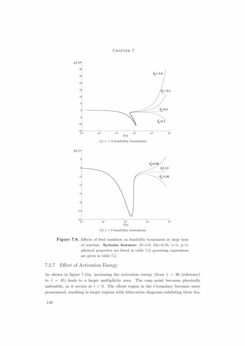
Chapter 7
10−3
10−2
10−1
100
101
102
−15
−10
−5
0
5
10
15
20
25
30
35
f [−]
q [−]
θ0* =0.0
θ0* =0.1
θ0* =−0.2
θ0* =−0.5
(a) v = 0 feasibility boundaries
10−2
10−1
100
101
102
−12
−10
−8
−6
−4
−2
0
2
4
θ0* =1.0
θ0* =0.95
θ0* =1.05
f [−]
q [−]
(b) l = 0 feasibility boundaries
Figure 7.8. Effects of feed condition on feasibility boundaries at large heat
of reaction. Systems features: B=1.0; Da=0.10; z=1; p=1;
physical properties are listed in table 7.3; governing expressions
are given in table 7.2.
7.2.7 Effect of Activation Energy
As shown in figure 7.10a, increasing the activation energy (from γ = 30 (reference)to γ = 45) leads to a larger multiplicity area. The cusp point becomes physicallyunfeasible, as it occurs at l < 0. The elbow region in the l-boundary becomes morepronounced, resulting in larger regions with bifurcation diagrams exhibiting three fea-
140

Steady and Dynamic Behavioral Analysis
sibility boundaries.
7.2.8 Effect of Relative Volatility
In the reference case, the relative volatility α (=p01/p
02) has a large value (≈ 8). As
reported in the case of synthesis of ethylene glycol by RD (Ciric and Miao, 1994),high volatility contributes to state multiplicity. The effect of reducing the relativevolatility is addressed in this subsection. A value of α=4.4 is considered, keeping allother parameters at their reference value. As depicted in figure 7.10b, the extent ofthe multiplicity region becomes smaller than that in the reference case (cf. figure 7.3).Moreover, the feasibility boundaries are less relevant, as the elbow region on the l-boundary disappears and the region between the turning points on the v=0 curve isquite small.
The effect of increasing reaction heat and activation energy and decreasing relativevolatility is illustrated in figure 7.11. The multiplicity area remains small with respectto the reference case, but the feasibility boundaries become more significant. Lakerveldet al. (2005) report bifurcation diagrams that exhibit up to five feasibility boundaries.
10−2
10−1
100
101
−2
−1
0
1
2
3
4
f [−]
q [−]
unfeasibleregion
l=0
feasibleregion
MSSregion
unfeasibleregion
v=0
T
T
H
Figure 7.9. Effects of heat of reaction on codimension-1 singular points.
Nomenclature: H : hysteresis variety (cusp loci); T : turning
point loci. Systems features: B=1.0; Da=0.10; z=1; p=1;
θ∗0=0.13; physical properties are listed in table 7.3; governing ex-
pressions are given in table 7.2.
141

Chapter 7
10−1
100
101
102
−10
0
10
20
30
40
50
f [−]
q [−]
unfeasibleregion
unfeasibleregion
v=0
MSSregion
T
Tfeasibleregion
H
l=0
(a) Large activation energy, γ=45
10−1
100
101
−0.2
0
0.2
0.4
0.6
0.8
f [−]
q [−]
unfeasibleregion
l=0
H
TT
MSSregion
unfeasibleregion
v=0
feasibleregion
(b) Smaller relative volatility, α=4.4
Figure 7.10. Effects of activation energy and relative volatility on
codimension-1 singular points. Nomenclature: H : hysteresis
variety (cusp loci); T : turning point loci. Systems features:
Da=0.10; z=1; p=1; θ∗0=0.13; physical properties are listed in
table 7.3; governing expressions are given in table 7.2.
7.2.9 Significance of Results and Extension Possibilities
The results of this section show that a considerable number of bifurcation diagrams canbe identified even for a simplified RD application. By addressing a single reactive traywe aim to explore exclusively the interaction between phase equilibrium and chemicalreaction. The possibilities to extend this approach to a more realistic and full-scale RD
142

Steady and Dynamic Behavioral Analysis
system are numerous.
10−2
10−1
100
101
102
−60
−40
−20
0
20
40
60
f [−]
q [−]
unfeasibleregion
l=0
H
TT
MSSregion
unfeasibleregion
v=0
feasibleregion
Figure 7.11. Combined effects of heat of reaction, activation energy and rel-
ative volatility on codimension-1 singular points. Nomencla-
ture: H : hysteresis variety; T : turning point loci. Systems
features: B=5; γ=50; α=4.4; Da=0.10; z=1; p=1; θ∗0=0.13;
physical properties are listed in table 7.3; governing expressions
are given in table 7.2.
For instance, the idealized physical properties of the system could be replaced by rate-limited mass/heat transfer models, as suggested by Baur et al. (2001c); Higler et al.(1999b). Multiplicity behavior is reported in both models for the case of MTBE syn-thesis and only differing in the relative size of region of occurrence. Additionally, ifwe extend our reactive tray to a RD column with reactive and nonreactive sections,the effect of both regions on MSS occurrence should be borne in mind. As mentionedby (Guttinger and Morari, 1997), these interactions could be largely responsible formultiplicity. In both cases, singularity theory approach could be useful to investigatethe main behavior patterns. The approach presented in this section is not restrictedto our case study but could be equally applicable to more complex reactive distillationsystems, including multicomponent, multireaction and nonideal systems.
143

Chapter 7
7.3 Dynamic Behavior
7.3.1 Introduction
The nonlinear coupling of reactions, transport phenomena, phase equilibria and hard-ware hydraulics can give rise to highly complicated dynamic behavior of the system. Inthe previous section, we showed that even for a simplified reactive flash and an idealizedsystem a large number of bifurcation diagrams could be identified. The main source ofmultiplicity is then suggested to be the strong nonlinear coupling of reactions, transportphenomena and phase equilibria.
The strong parametric sensitivity resulting from this coupling largely determines thestart-up procedure, steady-state and transient operations (Ruiz et al., 1995). Moreover,even small variations in the input variables might lead to unstable conditions (Alejskiand Duprat, 1996). This fact implies that a feasible operation of a RD column requiresseveral control loops to mitigate the effects of disturbances.
In this section, we explore the process dynamics of a full RD unit. The scope of thisanalysis is restricted to a limited version of control system design, as a SISO structureand PID controllers are a priori selected. The starting point of the analysis involves thedevelopment of a reliable mathematical model, capable of predicting with acceptable ac-curacy the unit behavior. Moreover, the model should not be computational expensiveat this conceptual design level. To identify the variables to be controlled and manipu-lated and then fully analyze the dynamic behavior of the system a rigorous degree offreedom analysis is performed. Moreover, the controllers have to be effectively tunedand a realistic disturbance scenario has to be defined. The analysis of the unit involvesassessing its capability of coping with the disturbance scenario without violating thespecification constraints. It is worth mentioning that this approach does not addressany interaction between column design and control design.
The content of this rather classical control approach sets the stage for a next novelcontribution to be introduced in chapter 8, involving the trade-off between design,responsiveness and sustainability aspects. Thus, the outcome of this section serves asa reference case to be compared with that of the life-span inspired design methodology(cf. section §1.4).
As in previous chapters, the synthesis of MTBE is used as case study. As the focusof this section is the dynamic behavior of the unit around a desired steady state, wechoose appropriate processing conditions and design parameters to avoid multiplicity asmuch as possible. The steady state of interest is the high-purity one as given elsewhereHauan et al. (1995a,b); Jacobs and Krishna (1993); Schrans et al. (1996).
144

Steady and Dynamic Behavioral Analysis
7.3.2 Model Description, Control Structure and Disturbance Scenarios
7.3.2.1 Model Description
A RD column is considered for modeling and analysis purposes. During the modeldevelopment of this unit the following set of assumptions are made: (i) the liquid andvapor streams leaving a trays are in thermodynamic equilibrium; (ii) both liquid andvapor hold-ups are fully considered; (iii) the liquid and vapor on each tray are perfectly-well mixed (i.e. no radial gradient in temperature and composition and the liquid onthe tray has a concentration equal to that of the liquid leaving the tray); (iv) thereactions are taking place in the liquid phase and enhanced by a solid catalyst; (v) thereactions occur only on the trays containing catalyst; (vi) vapor and liquid entrainmentis neglected; (vii) the column is equipped with a condenser, reflux drum and reboiler;(viii) the location(s) of the feed stream(s) and product stream(s) are known a priori; (ix )the sizing parameters of the unit and operational variables are obtained from previousdesign stages (cf. section §6.2); (x ) the liquid hold-up on a tray is related to theliquid outflow according to Francis weir formula; (xi) the flow of vapor leaving a tray isdetermined by the pressure drop between two consecutive trays; (xii) the tray pressuredrop includes contributions of dry pressure drop, liquid height (weir height plus heightover the weir) and residual head; (xiii) the physical properties of the involved streamsare computed as a function of temperature and/or phase composition; (xiv) the heatof reaction is omitted in the energy balance, because the heat of formation at standardconditions (1.033 ·105 Pa/298 K) is used as reference in the enthalpy computations; (xv)the reboiler, condenser and reflux drum are nonreactive units; (xvi) the tray sizing isestimated by rules-of-thumb criteria (Coulson and Richardson, 1991); (xvii) the columndiameter is larger than the minimum flooding value.
The RD model consists of sets of algebraic and differential equations, which are obtainedfrom the mass, energy and momentum balances performed on each tray, reboiler, con-denser, reflux drum and PI controller instances. Additionally, algebraic expressions areincluded to account for constitutive relations and to estimate physical properties of thecomponents, plate hydraulics and column sizing. Moreover, initial values are includedfor each state variable. A detailed description of the mathematical model can be foundin appendix A. The model is implemented in gPROMS c©/gOPT c©and solved using forthe DAE a variable time step/variable order Backward Differentiation Formulae (BDF).
A rigorous degree of freedom analysis is performed to asses the consistency of the modeland identify the set of controlled and manipulated variables. According to this analysis(tables A.1-A.3 in appendix A), the following set of input variables should be fixed,
• the reflux ratio, RR
• the RD column diameter at each location, nt × Dcol,
145

Chapter 7
Table 7.4. Optimized design of a RD column for MTBE synthesis as obtained
in chapter 6.
Value
Number of trays 15 [2:rectifying;8:reactive; 5:stripping]
Feed 1: location iC4+ nC4 : 10th tray (g)Feed 1: flowrate 455 mol×s−1
Feed 1: composition iC4 : 0.37; nC4 : 0.63Feed 1: temperature 350KFeed 2: location MeOH: 9th tray (l)Feed 2: flowrate 168 mol×s−1
Feed 2: composition MeOH: 1.00Feed 2: temperature 320KOperating pressure 11·105 Pa (top)Reflux ratio 7Mass of catalyst/tray 204.1 kg=1000 eq[H+]
Bottom flowrate 197 mol×s−1
Column diameter 7.132 mCondenser area 1.059·103 m2
Reboiler area 6.93·102 m2
MTBE bottom fraction 0.990-0.998
• the condenser area, Acond, and
• the reboiler area Areb.
The synthesis of MTBE from a C4-stream and methanol in the presence of an acidiccatalyst is used as tutorial application. A detailed description of this system is availablein appendix B. The spatial structure of the RDC is that obtained by optimization inchapter 6 and summarized again in table 7.4. Discrete variables are arbitrarily fixedfor the sake of simplicity. Thus, the structural configuration (i.e. number of traysand streams’ staging) used in this example corresponds to the one used by Jacobs andKrishna (1993); Hauan et al. (1995a); Seader and Henley (1998). The values of thesevariables are also included in table 7.4.
7.3.2.2 Control Structure
To mitigate any effect caused by a disturbance scenario a control structure is proposedfor the RD unit depicted in figure 7.12. The following assumptions are considered: (i)four control valves are associated with the RD unit; (ii) the unit is operated at constantreflux ratio RR (=FR,L/FD,L=7); and (iii) the throughput of the unit is set.
146
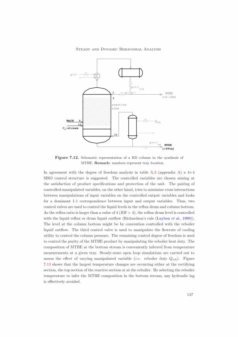
Steady and Dynamic Behavioral Analysis
1
15
9
10
MeOH
C4-stream
���������
3
MTBE(>99%m)
MTBE(<0.1%m)
reactivezone
Fcool
Qreb
Fout,Lcond
Fout,Lreb
FR,L FD,L
Figure 7.12. Schematic representation of a RD column in the synthesis of
MTBE. Remark: numbers represent tray location.
In agreement with the degree of freedom analysis in table A.3 (appendix A) a 4×4SISO control structure is suggested. The controlled variables are chosen aiming atthe satisfaction of product specifications and protection of the unit. The pairing ofcontrolled-manipulated variables, on the other hand, tries to minimize cross interactionsbetween manipulations of input variables on the controlled output variables and looksfor a dominant 1-1 correspondence between input and output variables. Thus, twocontrol valves are used to control the liquid levels in the reflux drum and column bottom.As the reflux ratio is larger than a value of 4 (RR > 4), the reflux drum level is controlledwith the liquid reflux or drum liquid outflow (Richardson’s rule (Luyben et al., 1999)).The level at the column bottom might be by convention controlled with the reboilerliquid outflow. The third control valve is used to manipulate the flowrate of coolingutility to control the column pressure. The remaining control degree of freedom is usedto control the purity of the MTBE product by manipulating the reboiler heat duty. Thecomposition of MTBE at the bottom stream is conveniently inferred from temperaturemeasurements at a given tray. Steady-state open loop simulations are carried out toassess the effect of varying manipulated variable (i.e. reboiler duty Qreb). Figure7.13 shows that the largest temperature changes are occurring either at the rectifyingsection, the top section of the reactive section or at the reboiler. By selecting the reboilertemperature to infer the MTBE composition in the bottom stream, any hydraulic lagis effectively avoided.
147

Chapter 7
2 4 6 8 10 12 14 16
350
360
370
380
390
400
410
420
430
440
+ 0.5% Qreb
- 0.5% Qreb
base case
Treb
[K]
Tray location [-]
Figure 7.13. Effect of reboiler heat duty on the temperature profile in an
MTBE RD column. Remarks: trays are numbered from top
(condenser: 1st) to bottom (reboiler: 1st); MTBE product
stream is withdrawn from the bottom location; column speci-
fications are listed in table 7.4 .
This single-end point composition control structure is originated from the assumptionof invariant reflux ratio. As mentioned by Luyben et al. (1999), this control structure isadvantageous from both operational (i.e. easy tuning) and economical (i.e. comparableenergy consumption) point of view compared to a dual composition control. The overallcontrol structure is labelled [RR] − Qreb, meaning that the reflux ratio is fix and thereboiler heat duty is used to control the bottom stream purity. Figure 7.14 depictsthe proposed control structure and table 7.5 details each control loop. The controllersare tuned according to the guidelines presented in section §6.2.3.2. Table 6.5 lists allcontrollers parameters obtained using optimization and adopting a sequential approach(i.e. optimization of sizing parameters followed by optimization of control parameters).The controllers are assumed to be correctly tuned. Alternative control configurationsare proposed for the MTBE synthesis by Wang et al. (2003); Sneesby et al. (1998b)addressing switch-over to different steady states. As the focus of this section is thedynamic behavior around a known steady state, no steady-state transition is consideredby constraining the disturbances’ variability.
148

Steady and Dynamic Behavioral Analysis
1
15
9
10
MeOH
C4-stream
3
MTBE(>99%m)
MTBE(<0.1%m)
reactivezone
P
L
L
T
Fcool
Pcond
levelcond
levelreb
Treb
Qreb
Fout,Lcond
Fout,Lreb
FR,L FD,L
Figure 7.14. Schematic representation of a MTBE RD column with a 4×4
SISO control structure. Remarks: the coupling between con-
trolled and manipulated variables for each control loop are listed
in table 7.5; numbers represent tray location.
Table 7.5. Control loops in a reactive distillation stage column. The schematic
representation of the unit is given in figure 7.14.
Unit Controlled variable Manipulated variable
P1 Liquid level in condenser,levelcond
Outgoing flowrate in condenser,F out,L
cond
P2 Pressure in condenser, Pcond Flowrate of cold utility in con-denser, F cool
P3 Liquid level in reboiler, levelreb Outgoing flowrate in reboiler,F out,L
reb
P4 Temperature in reboiler, Treb Heat duty of hot utility in re-boiler, Qreb
149

Chapter 7
0 20000 40000 60000 80000 100000282
284
286
288
290
292
294
Tin,cool [K]
Time [s]
(a) Disturbance in the inlet temperatureof the cold utility, T in,cool, as defined inequation 7.1. Time horizon=86400 s.
0 10000 20000 30000 40000 50000 60000166
168
170
172
174
176
178
180
182
184
186
FMeOH
[mol/s]
Time [s]
(b) Disturbance in the feed flowrate ofmethanol, FMeOH, as defined in equation
7.2. Time horizon=60000 s.
Figure 7.15. Disturbance scenarios considered for the analysis of the dynamic
behavior of a MTBE RD column. Remark: column specifica-
tions are listed in table 7.4.
7.3.2.3 Disturbance Scenarios
In addition to the disturbance scenarios already defined in section §6.2, two disturbancesare considered for this behavioral analysis (figure 7.15),
• a sinusoidal variation of coolant inlet temperature during 24 h (=86400 s) anddefined as,
T in,cool = 298 + σs(t), with σs(t) := 5× sin(2× π
8.64 · 104× t). (7.1)
• a step variation in the flowrate of methanol during the time horizon of 6·104 s anddefined as,
FMeOH =
F
SSMeOH if t < 1 · 104 s or t > 4 · 104 s,
1.1× FSSMeOH if 4 · 104 s > t > 1 · 104 s.
(7.2)
It is relevant to mention that the disturbance scenarios are defined in such a waythat multiplicities are avoided. Since a detailed MSS analysis in RD has been alreadyaddressed in section 7.2.1, this section focuses exclusively on the dynamic behavior ofthe RD unit around an already known steady state. Thus, the control structure isdefined so that no steady-state transitions are occurring. The effect of large methanolfeed disturbances (∆FMeOH > 0.1) on the operational steady state has been covered bySchrans et al. (1996); Sneesby et al. (1998a,b).
150

Steady and Dynamic Behavioral Analysis
2 4 6 8 10 12 14 160.0
0.2
0.4
0.6
0.8
1.0
Wang et al. (2003)
this work
xMTBE
[-]
Tray location [-]
(a) MTBE composition profile.
2 4 6 8 10 12 14 16340
350
360
370
380
390
400
410
420
430
Wang et al. (2003)
this work
Temperature [K]
Tray location [-]
(b) Temperature profile.
Figure 7.16. Comparison between steady-state profiles obtained in this work
and by Wang et al. (2003). Remarks: trays are numbered
from top (condenser: 1st) to bottom (reboiler: 17th ); MTBE
product stream is withdrawn from the bottom location; column
specifications are listed in table 7.4.
7.3.3 Dynamic Response in the Presence of Disturbances
A preliminary analysis of the RD model is performed in the absence of any disturbancescenario. For the sake of model validation, the profiles of MTBE molar fraction andstage temperature are compared with those reported by Wang et al. (2003).
As noticed from figure 7.16 a relatively good agreement exists between both simulations.In the temperature profile, however, a slight difference is reported in the rectifying andreactive sections of the unit. The origin of this mismatch could be attributed to thedifferent inert component considered in both cases. Wang et al. (2003) assume that theC4-stream contains n-butene as inert component, whereas in the course of this thesiswork inert n-butane is used. The different physical properties of these componentsmight be leading to slightly altered energy balances and subsequently to different traytemperature. As the temperature mismatch starts to play a role on the reactive trays,it could be suggested that differences exist between the estimations of reaction heat.Moreover, the kinetic and thermodynamic models used in both cases do not fully co-incide. On the other hand, the degree of agreement between MTBE molar fractionsobtained by Wang et al. (2003) and this work is quite satisfactory.
At this point the dynamic behavior of the RD unit is analyzed with respect to dis-turbance rejection. Figure 7.17 depicts the evolution of MTBE bottoms compositionin presence of the deterministic disturbances. Oscillations around the set-point valueare noticed, but of extremely small magnitude σ, specially for the disturbance in the
151

Chapter 7
0 20000 40000 60000 80000 1000000.000.020.040.060.08
0.99760
0.99762
0.99764
0.99766
0.99768
0.99770
0.99772
0.99774
0.99776
0.99778
0.99780
xMTBE
[-]
Time [s]
(a) T in,cool disturbance scenario. Timehorizon: 8.64·104 s.
0 10000 20000 30000 40000 50000 600000.000.020.040.060.08
0.995
0.996
0.997
0.998
0.999
1.000
xMTBE
[-]
Time [s]
(b) FMeOH disturbance scenario. Timehorizon: 6·104 s.
Figure 7.17. Time variation of MTBE product stream in the presence of de-
terministic disturbance scenarios. Remarks: MTBE product
stream is withdrawn from the bottom location; the column spec-
ifications are listed in table 7.4.
coolant inlet temperature,
• |σ| < 0.002% for the T in,cool disturbance
• |σ| < 0.2% for the FMeOH disturbance
After the disturbances the RD column returns to its initial state, without any steady-state transition. From these results it can be suggested that the unit operates copingwith product specification in spite of the presence of the defined disturbances. Ob-viously, more aggressive disturbance scenarios might lead to unit instability or evensteady-state transitions. Schrans et al. (1996); Sneesby et al. (1998a,b) show that in-stabilities are expected to occur at slightly higher methanol flow disturbances.
7.4 Concluding Remarks
The conclusions derived from this chapter are grouped in accordance to the presentedsections.
Steady-state behavior. In this first section, a reactive flash with a rather idealsystem (mildly exothermic isomerization reaction and light-boiling reactant) was con-sidered. This simplified system was selected to account exclusively for the effect ofphenomena interaction on the occurrence of input and output multiplicity. Therefore,any effect related to unit configuration is considered outside the scope of the analysis.
152

Steady and Dynamic Behavioral Analysis
For this particular case, the number and relative location of the turning points andfeasibility boundaries corresponding to no-liquid or no-vapor products determined thequalitative nature of the bifurcation diagram. State multiplicity was present in a largearea of the parameter space, for the case under consideration. A large number (25)of qualitatively different bifurcation diagrams could be identified for the system. Thefeasibility boundaries played an important role in the classification of the reactive flash.Up to five feasibility boundaries and a maximum of 3 steady states were found in asingle bifurcation diagram. Bifurcation diagrams exhibiting more then two feasibilityboundaries are common for liquid or vapor feed. Increasing the heat of reaction, ac-tivation energy or relative volatility enlarges the area of multiplicity. Furthermore, alarge heat of reaction can create regions in parameter space with 5 feasibility bound-aries in a single bifurcation diagram. The singularity theory approach could be usefulto investigate the main behavior patterns in more complex reactive distillation systems,including multicomponent, multireaction and nonideal systems. Moreover, the effect ofmass transfer would be worthwhile to examine, having as initial step the contributionsof Baur et al. (2001c); Higler et al. (1999b).
Dynamic behavior. The second part of this chapter deals with the dynamic be-havior of a full RD column, with special focus on the synthesis of MTBE. The contentof this rather classical control approach (SISO and PI controller) sets the stage for anext novel contribution to be introduced in chapter 8, involving the trade-off betweendesign, responsiveness and sustainability aspects. A generic dynamic model was de-veloped for a complete RD column. The model was composed of instances of (non-)reactive trays, condenser, reflux drum, reboiler and PI controllers. Based on a rigorousdegree of freedom analysis and engineering judgement a control structure was defined.The synthesis of MTBE was used as tutorial example for this section. The sizing ofthe unit corresponded to the optimized values obtained in previous chapters (cf. chap-ter 6). A set of deterministic disturbances were included, accounting for a sinusoidalvariation of coolant inlet temperature and a methanol feed flowrate pulse. Moreover,the disturbances were defined in such a way that steady-state transitions were avoided.The controllers were tuned based on the optimization of the integral absolute error(cf. section §6.2.3.2). To first validate the model, a comparison was made between theprofiles obtained in this work and those reported in literature. A satisfactory degree ofagreement was noticed. When the unit was dynamically simulated in the presence ofthe disturbances scenarios, minor variations in the MTBE bottom fraction were found.As the magnitude of these set-point deviations was very small, it is suggested that theunit operates under product specifications in the presence of the defined disturbancescenarios. Thus, the outcome of this section serves as a reference case to be comparedwith that of the life-span inspired design methodology (cf. section §1.4).
153

Chapter 7
Mind journey to the scientific questions.
The steady-state and dynamic behavior in RD are addressed inthis chapter. Fundamental understanding of multiplicity in a re-active flash is provided. Moreover, the domain knowledge is ex-tended by dynamic analysis, whose tasks include model develop-ment, control structure selection, controller tuning and simulationof closed loop dynamics. The output of this section serves as ref-erence case to be compared with that of the life-span inspireddesign methodology (cf. section §1.4). The material presented inthis chapter answers partially Question 6.
154

“It is not the strongest of the species that survive, nor the
most intelligent, but the one most responsive to change.”
Charles Darwin, naturist (1809-1882)
8A Design Approach Based on Irreversibility†
The interactions between economic performance, thermodynamic efficiency and re-
sponsiveness in RD process design are explored in this chapter. This motivation is de-
rived from taking a sustainable life-span perspective, where economics and avoidance
of potential losses of resources (i.e. mass, energy and exergy) in process operation
over the process life span are taken into consideration. The approach to the column
design involves defining a building block, generic lumped RD volume element and
the development of rigorous dynamic models for the behavior of the element. As an
extension of conventional existing models, this model, which is used as a standard
building block, includes entropy and exergy computations. Three objective functions
are formulated which account for the process performance regarding economy, exergy
loss and responsiveness. A fundamental understanding of the strengths and short-
comings of this approach is developed by addressing a case study: (i) steady- state
simulation of a classical MTBE design based on economics only, useful as a refer-
ence case; the multiobjective optimization of a MTBE RD column with respect to
(ii) economics and thermodynamic efficiency; and (iii) economics, thermodynamic
efficiency and responsiveness. Finally, structural differences and dynamic response
are identified between the optimized and classical designs, to stress the importance
of considering exergy and responsiveness criteria.
†Parts of this chapter have appeared in Almeida-Rivera et al. (2004b)
155

Chapter 8
8.1 Introduction
Advances in computing and information technology allow chemical engineers to solvecomplex design problems arising from a need to improve sustainability of the biosphereand human society. In such a context the performance of a chemical plant needs tobe optimized over its manufacturing life span, while accounting for the use of multipleresources in the design and manufacturing stages. Since such resources are of a differentnature (e.g. capital, raw materials and labor) with different degrees of depletion andrates of replenishment the performance of a chemical plant is characterized by multipleobjectives with trade-offs. An integrated unit operation like RD can offer significantbenefits for resource utilization, when it is accompanied with the avoidance of chemicalequilibrium limitations, enhancement of conversion, selectivity and yield and the reduc-tion of both operational and capital costs. The nonlinear coupling of chemical reaction,phase equilibria and transport phenomena can however, leads to undesired, system-dependent features, such as multiple steady states and reactive azeotropes (Malone andDoherty, 2000). The results of a case study on the interactions between economics,exergy efficiency and process responsiveness in the conceptual design of RD processesare discussed in this chapter.
In the wider context of conceptual process design, sustainability issues like feedstockselection, (re-)use of catalyst and (re-)use of solvents are of key importance. In ourperspective of life span (cf. explanatory caveat in section §1.4), we do not cover thoseaspects as we focus exclusively on the minimization of loss of resources in the operationalphase.
Currently, conceptual design in chemical engineering is predominantly driven by (steadystate) economic considerations, postponing to latter engineering stages any issue relatedto exergy analysis, responsiveness and control performance. The importance of incorpo-rating exergy efficiency in the early stages of the design cycle is stressed by the increasingdepletion of nonrenewable energy resources and the relatively low second law efficiencies(5-20%) for the majority of chemical processes. In spite of these facts, exergy analysis isexclusively performed as a follow-up task to the process synthesis (Koeijer et al., 2002).Controllability and process responsiveness are important to maintain product qualityand to avoid excessive use of utilities for control actions and reprocessing of off-specmaterial.
Regarding the multiechelon approach in RD design (cf. chapter 4) in this chapter thelast design space is addressed. The evaluation of the design obtained so far is checkedwith respect to economic performance, exergy efficiency and responsiveness. The focusof this chapter is the importance of including interactions between economics, exergyefficiency and process responsiveness in RD conceptual design. Aiming at these goals,a generic compartment model is defined, which accounts for mass, energy and momen-
156

A Design Approach Based on Irreversibility
Table 8.1. Input-output information for the thermodynamic-based evaluation
space. The multiechelon approach is explained in section §4.5.
Design specifications Design/operational variables Domain knowledge
Process: Continuous: - non-equilibrium
- spatial configuration - optimal design variables thermodynamics
- control structure and settings - performance criteria - steady-state simulation
- operational parameters - dynamic simulation
- disturbance scenario - multiobjective optimiza-
tion
tum balances and includes entropy and exergy computations. This behavioral modelis integrated to give a column structure. The design is cast into a nonlinear optimiza-tion problem, where degrees of freedom in the design model are fixed by optimizationof multiple objectives and applying constraints, reflecting heuristics and engineeringknowledge. At this column level three performance criteria are defined for the opti-mization of the unit design. These embrace the unit performance regarding economics,thermodynamic efficiency and process responsiveness. The economic performance in-dex is given by the total annualized cost (TAC), whereas the thermodynamic efficiencyindex accounts for the process irreversibilities and is expressed in terms of the entropyproduction rate by chemical reaction, heat and mass transfer. The responsiveness in-dex, in turn, is similar to the response time defined by Luyben et al. (1999). Thethree objective functions are solved simultaneously within a single multiobjective opti-mization problem. At this level of understanding, it is believed that a multiobjectiveoptimization gives more insight into trade-offs between objectives than combining thethree objectives into a single monetary objective function using ad-hoc weighting fac-tors. Comparing the design based on the three-fold performance criteria with a referenceeconomic-driven design allows us to identify structural differences. The response of theoptimized design in the presence of a deterministic disturbance scenario is validatedusing dynamic simulation.
The input-output flow of information is given in table 8.1. It is worth mentioning thatthe thrust of this chapter is the optimization-based design approach. Multiple objectivefunctions are considered and embedded in a large scale optimization problem.
Recalling the engineering and scientific design questions given in chapter 1, in thischapter we address question 7, namely,
• Are there structural differences and significant improvements in designs derivedusing conventional methodologies from those obtained using an integrated designmethodology?
157

Chapter 8
8.2 Generic Lumped Reactive Distillation Volume Element
The starting point for a fundamental understanding of the strengths and shortcom-ings of the proposed multiobjective design approach is to define a generic lumped RDvolume element (GLRDVE) . This element, or compartment, was chosen as buildingblock in the design approach (cf. section §6.1.3) and selected to represent the govern-ing phenomena occurring in RD processing. Thus, this behavioral model accounts for:(i) mass, energy and momentum balances, together with entropy and exergy computa-tions; (ii) thermodynamic equations of state for the specific heat and specific densityand for the chemical potential per species; (iii) thermodynamic phase equilibrium con-ditions at the contact surface between phases; (iv) the constitutive rate equations forchemical reactions; (v) the rate equations for interphase transport of species mass andenergy; (vi) the rate equation for heat transfer with an external solid surface; (vii) thehydrodynamics-based rate equations for convective mass and energy flows with the ex-ternal world and the pressure drop; and (viii) the equations for the interphase contactsurfaces and for the void fraction of the vapor phase in the liquid phase.
The following attributes are introduced: (i) two internally (well mixed) homogeneousfluid phases; and (ii) chemical reactions in the liquid phase only. Thus, mass transfer be-tween phases and heat exchange are allowed in the compartment and chemical reactionis triggered by the presence of an appropriate catalyst (figure 8.1). Each GLRDVE hasits own complexities due to the many interacting phenomena. However, this does notaccount for the interactions between the stages in a real multistage column. The latterclass of interactions could give rise to nonlinear dynamic behavior and poor controlla-bility if an unfortunate combination of reflux ratio and number of (non) reactive traysis chosen. Issues related to connecting compartments and superstructure descriptionare addressed in section §8.3.
8.2.1 Mass/Energy/Entropy/Momentum balances
Component, energy and entropy balances are developed in the GLRDVE. The entropyand, in particular, the entropy production rate are of paramount importance to de-termine exergy losses and the responsiveness of the process. The balances lead to thefollowing set of DAEs,
158

A Design Approach Based on Irreversibility
Q
F feed,Vn
Rx
F Vn+1
F side,Vn
F Vn
F feed,Ln
F Ln
F Ln-1
F side,Ln
Figure 8.1. Schematic representation of the generic lumped reactive distilla-
tion volume element (GLRDVE). Remark: feed and side draw-
off streams and heat exchange are allowed. Nomenclature:
Ffeed,(α)i : feed flowrate of phase (α); F side,(α): flowrate of side
stream corresponding to phase (α); Ψm: interfacial mass transfer
flux; Ψe: interfacial energy transfer flux; Q : heat duty.
∂(ρ(α)i × V (α)
)∂t
=j=nst∑j=1
Fj,(α)i − Ψi × aΨ + δ(α) × ri × V L
RX , i ∈ Znc , (8.1)
∂U(α)
∂t=
j=nst∑j=1
i=nc∑i=1
Fj,(α)i × h
j,(α)i + Ψe × aΨ + · · ·
· · · +j=nst∑j=1
i=nc∑i=1
Fj,(α)i × g
j,(α)i + δ(α) × Q(α), (8.2)
where c(α)i is the molar density of component i (i ∈ Znc) in phase (α) ∈ Znp , F j,(α)
i
is the convective flow of component i in phase (α) in the incoming or outgoing streamj (j ∈ Znst) for the exchange with the external world, Ψi is the interfacial molar fluxof component i, aΨ is the mass and heat transfer area, V L
RX is the reaction volume inthe liquid phase, rj is the net cumulative rate of reaction of specie j per unit, U isthe internal energy of the compartment, hj,(α)
i is the molar enthalpy of component i instream j and phase (α), gj,(α)
i is the external force exerted on component i per molarunit (including the contribution from electrical field) in stream j and phase (α), Ψe isthe energy flux associated with the interface mass and heat transfer, Q(α) is the externalheat exchange rate in phase (α), which is assumed to only occur in the liquid phase(i.e. Q(α) = QL), nc is the number of components, nst is the number of incoming and
159

Chapter 8
outgoing streams, np is the number of phases and δ(α) is the Kronecker delta functiondefined as,
δ(α) :=
0, if (α) �= L
1, if (α) = L.(8.3)
The energy flux associated with the interface mass and heat transfer Ψe is composedof a measurable heat flux and the partial molar enthalpies brought by the componentfluxes. namely,
Ψe = −i=nc∑i=1
Ψi × h(α)i + q(α
′−α), (8.4)
where q(α′−α) is the heat flux from phase (α′) to phase (α).
The entropy balance in the transient state at a macroscopic level is given by the netamount of entropy transferred into the volume element per unit time and the amount ofentropy used/produced in the control volume per unit time. Thus, the entropy balancefor a given phase (α) can be stated as,
∂S(α)
∂t=
i=nst∑i=1
j=nc∑j=1
Fi,(α)j × s
i,(α)j + Σ(α)
V , (8.5)
where S(α) is the entropy of the compartment in phase (α), Si,(α)j is the molar entropy
of component j in stream i and phase (α) and Σ(α)V is the entropy production rate
in phase (α), which includes exclusively interfacial diffusional and chemical reactioncontributions.
Alternatively, the entropy balance can be expressed in terms of the entropy density andthe fluxes of entropy density (Kjelstrup and Bedeaux, 2001; Marquardt, 2004),
∂s(α)
∂t= −∇J (α)
s + σ(α)V , (8.6)
where σ(α)V is the entropy production rate per unit of volume in phase (α) and J
(α)s is
the entropy flux in phase (α).
The flux of entropy of stream i in phase (α) is related to the total flux of energy J i,(α)e
and mass fluxes J i,(α)m according to the expression (Kjelstrup and Bedeaux, 2001),
J i,(α)s =
1T
× J i,(α)e −
j=nc∑j=1
µi,(α)j
T× J
i,(α)m,j , i ∈ Z
nst , (8.7)
where µi,(α)j denotes chemical potential of component j (j ∈ Znc) in stream i and phase
(α).
160

A Design Approach Based on Irreversibility
The fluxes of mass and energy required in expression 8.7 can be obtained from theequation of continuity per volume unit and energy balance, respectively, for an openunsteady state multicomponent system. Let (α) be a given phase, then the funda-mental equation of continuity is given by convective, diffusive and chemical reactioncontributions,
∂
∂tρ(α)i = −(∇ρ(α)
i · v(α)) − (∇j(α)i )︸ ︷︷ ︸
−(∇·{ρ(α)i v(α)+j
(α)i })≡−∇J
(α)m,i
+r(α)i , i ∈ Z
nc , (8.8)
andJ(α)
m,i = ρ(α)i v(α) + j(α)
i , i ∈ Znc , (8.9)
where v(α) is the fluid velocity in phase (α) and the molar diffusion flux vector j(α)i
involves terms originated by mechanical and thermal driving forces (Bird et al., 2003).It is worth mentioning that the j(α)
i vector is composed of the elements jk,(α)i with
k ∈ Znst .
Similarly, the energy flux Ji,(α)e (J(α)
e in vectorial notation) can be obtained by theenergy equation derived for the volume element in an open multicomponent dynamicsystem,
∂
∂tu(α) = −(∇ · u(α)v(α)) − (∇q(α)) − (π(α) : ∇v(α))︸ ︷︷ ︸
−(∇·{u(α)v(α)+q+[π(α)·v(α)]})≡−∇J(α)e
+i=nc∑i=1
J(α)m,i · g(α)
i + E× j, (8.10)
where u is the internal energy density of the volume element, π(α) is the pressuretensor in phase (α), which accounts for the increase of the rate of internal energy byreversible pressure forces and by irreversible viscous forces (Bird et al., 2003), q(α) isthe multicomponent energy flux through the element interphase relative to the massaverage velocity in phase (α), E is the electric field and j the electric current density.
If it is assumed that the energy flux q(α) includes mainly conductive and interdiffusiveenergy fluxes (i.e. q(α) = qconductive + qdiffusive) and that the medium is isotropic, thetotal energy flux J(α)
e with respect to stationary coordinates is given, after eliminatingnegligible terms, by,
J(α)e = J(α)
q +i=nc∑i=1
J(α)i · h(α)
i , (8.11)
where Jq(α) is the measurable heat flux of phase (α).
The entropy production rate at macroscopic level, Σ(α)V (equation 8.5) can be obtained
after integration of the local entropy production rate density σ(α) over the volume ele-ment in phase (α). For the sake of simplification the following assumptions are adopted:(i) entropy contributions of all involving phases in the GLRDVE are combined in a sin-gle variable (Σ(∗)
V = f(Σ(α)V )); (ii) entropy is produced due to mass and heat diffusion in
161

Chapter 8
the liquid-vapor interphase, chemical reaction in the bulk of the liquid and heat transferfrom external heat sources/sinks and the surrounding environment to the liquid phaseonly; and (iii) the effects of electric field, external forces (g = 0) and diffusive momen-tum fluxes are neglected. The following expression for the integral entropy productionterm can be then derived (Seider et al., 1999; Bedeaux and Kjelstrup, 2004; Kjelstrupand Bedeaux, 2001),∫∫∫
V
σ(∗)dV =Σ(∗)V =
1TL
i=nrx∑i=1
ALi × εL
i × V LRX + JL
q × aΨ × Xq + · · · (8.12)
· · · +i=nc∑i=1
Ji × aΨ × hi × Xe +
(−
i=nc∑i=1
Ji × aΨ × Xm,i
)+ · · ·
· · · +Q× XHX ,
where ALi is the affinity of chemical reaction i (i ∈ Z
nrx) in the liquid phase, εLi is the
degree of advancement of chemical reaction i in the liquid phase, JLq is the measurable
heat flux into the liquid phase, aΨ is the mass/heat transfer area, hi is the molarenthalpy of component i, Xq, Xe, Xm,j and XHX are the conjugated driving forces forheat exchange between phases, interfacial heat diffusion, interfacial mass diffusion ofcomponent j and heat exchange with the external world, respectively (Koeijer et al.,2002), Q is the heat flow to the liquid phase, T is the absolute temperature of thevolume element and nrx is the number of chemical reactions.
The entropy contribution due to chemical reaction contains the affinity of chemicalreaction and its degree of advancement, which are defined respectively as,
ALj = −
i=nc∑i=1
νLi,j · µL
i , j ∈ Znrx , (8.13)
rLi =
j=nrx∑j=1
νLij × εL
j , i ∈ Znc , (8.14)
where rLi is the net change of the amount of component i in the liquid phase due to all
reactions.
In order to estimate the driving forces and fluxes occurring in the volume elementadditional assumptions are introduced: (i) the GLRDVE is composed of incoming andoutgoing streams of liquid and vapor phases; (ii) the vapor phase behaves ideally; (iii)the flux of mass and heat through the interface is positive from the liquid side to thegas side; (iv) dynamic changes in gas phase hold-ups of species mass and energy areignored; (v) Gibbs free energies at liquid and vapor sides are equal; and (vi) there is anegligible effect of pressure on Gibbs free energies, so that GL
i (P, T ) = GLi (p0
i , T ).
The underlying reasoning behind the inclusion of these assumptions is a more trans-parent derivation of the forces and fluxes expressions, but without compromising the
162
A Design Approach Based on Irreversibility
validity of the approach.
The driving force for chemical reaction j, Xrx,j, is a function of the chemical affinityand temperature, according to the expression,
Xrx,j =AL
j
T(8.15)
The flow associated to this driving force is given by the degree of advancement εi.The driving force for mass transfer Xm,i is related to the chemical potential gradientbetween the incoming and outgoing vapor streams (Koeijer, 2002; Kjelstrup, 2005).Thus, according to figure 8.1 the conjugated driving force Xm,i is,
Xm,i = − 1T
∆µi,T , i ∈ Znc , (8.16)
= R× lnyin
i × P in
yi × P, i ∈ Z
nc . (8.17)
The flux of component i (i ∈ Znc) associated to Xm,i through the interface can becalculated by mass balance over the vapor phase (Koeijer, 2002),
Ji × aΨ =j=nst∑j=1
F j,V × yji , i ∈ Z
nc , (8.18)
where yji denotes the vapor molar fraction of component i (i ∈ Znc) in stream j (j ∈
Znst) and F j,V is the total flow of stream j in the vapor phase and equals to F j,V =∑i=nc
i=1 F j,Vi .
Note that the previous flux expression is consistent with the component balance givenby expression 8.1 if Ψi equals Ji. Moreover, the total stream flow is related to thecomponent flow according to,
F j,V × yji = F j,V
i , i ∈ Znc . (8.19)
The driving force for heat transfer, Xe, can be estimated as suggested by Koeijer andRivero (2003),
Xe = ∆(
1T V
)=
12
(1
T out,V− 1T in,V
). (8.20)
The measurable heat flux through the interphase can be derived from the energy balancein the vapor side (Koeijer, 2002),
Je × aΨ =j=nst∑j=1
F j,V × hj,V . (8.21)
In this case also the energy expression 8.21 is consistent with the general energy balancegiven in expression 8.2 if Ψe equals Je.
163

Chapter 8
According to Koeijer et al. (2002); Koeijer (2002) the average thermal driving force forexternal heat transfer XHX (e.g. when a heat exchanger is present) is given by theexpression,
XHX =1T
− 2T u,in + T u,out
, (8.22)
where T u denotes temperature of the utility present in the GLRDVE.
The momentum balance in the GLRDVE involves, in its general form, contributionsdue to convection of the fluid bulk, pressure, viscous transfer and gravitational force ineach phase (Bird et al., 2003),
∂ρ(α) · v(α)
∂t= −[∇ · ρ(α) · v(α)v(α)] −∇P (α) − [∇ · ς] + c(α) · g(α), (8.23)
where ρ =∑i=nc
i=1 ρi, [∇ · ρ · v(α)v(α)] is the rate of momentum gain by convection ofthe fluid per unit volume and ∇ · ς is the rate of momentum gain by viscous transferper unit volume.
If viscous effects are considered unimportant the following simplified expression mightbe obtained,
∂ρ(α) · v(α)
∂t= −[∇ · ρ(α) · v(α)v(α)] −∇P (α) + ρ(α) · g(α). (8.24)
In the development of the GLRDVE a reduced form of the momentum balance is consid-ered. We assume a pseudo steady state and negligible viscous contribution. Moreover,the gradient of pressure is assumed to be much larger than the rate of momentum gainby convention of the fluid. Thus, the resulting momentum balance is of the form,
∇P (α) = ρ(α) · g(α). (8.25)
8.2.2 Availability and Availability Function
Two additional variable of key importance for this thermodynamic-based approach arethe availability A and the availability function B. The availability is regarded as ameasure of the maximum amount of useful energy that can be extracted when thesystem is brought to equilibrium with the dead state surroundings (Seider et al., 1999).Thus, the availability of the system in phase (α) and state (T1, P1) is given by theexpression,
A(α) = (h(α) − T0 × S(α))T1,P1 − (h(α) − T0 × S(α))T0,P0 , (8.26)
where the dead state conditions are those at which T0 = 298.15K and P0 = 1 atm.
The availability function at state given by (T, P ) is computed according to the followingequality,
B(α)T,P = (h(α) − T0 × S(α))T,P . (8.27)
164

A Design Approach Based on Irreversibility
Contrary to the availability the availability function of the system at a given state(T1, P1) can be referenced to any other state (T2, P2),
∆B(α) = (h(α) − T0 × S(α))T1,P1 − (h(α) − T0 × S(α))T2,P2 (8.28)
From the definitions of availability and availability function it should be noticed thatboth variables increase with increasing enthalpy and decrease with increasing entropyand the numerical values of their variation coincide (i.e.∆B(α) = ∆A(α)).
Based on the combination of energy and entropy balances and according to the definitionof availability an exergy balance can be obtained for a given phase (α) (appendix A inLuyben et al. (1999)),
∂B(α) ×M (α)
∂t=
j=nst∑j=1
F j,(α) × Bj,(α) +(
1 − T0
TQ
)Q(α) − T0 × ΣV , (8.29)
where M (α) is the molar hold-up of material in phase (α) and TQ is the temperature ofthe heat source/sink. Note that in the previous expression the external force term hasbeen omitted.
To solve the set of balances mentioned in this section it is necessary to specify the initialconditions for all DAEs. Thus, the following variables per phase should be known,
[ρ(α)i (0), U (α)(0), S(α)(0), ρ(α)(0) · v(α)(0), B(α)(0) ·M (α)(0)]. (8.30)
A degree of freedom analysis should be then performed to indicate how many designdecision variables need to be picked per volume element. Appendix A gives a detailedoverview of a degree of freedom analysis for the case of a complete RD column.
8.2.3 Design Decision Variables
According to a degree of freedom analysis performed in the GLRDVE the followingdesign variables are to be specified for a given operating conditions and feed specifica-tions,
• reaction volume V (α)RX ,
V(α)RX =
V
(α) for liquid phase homogeneously catalyzed reaction(s)
mcat × ρ−1m,cat for heterogeneously catalyzed reactions(s)
• external and heating/cooling flowrate Q,
• the interfacial area for heat and mass transfer aΨ.
165
Chapter 8
Note that operational variables such as reflux ratio and pressure are fixed at appropriatereference value and the connecting streams and associated flowrates F j,(α)
i are assumedto be given.
The perspective adopted for selecting the design decision variables is task-orientedrather than the conventionally used equipment-oriented design approach. Firstly, thetask-based concept would allow us to derive the phase volume V (α) from the reactiontime (i.e. residence time in element) to meet a specified degree of advancement ofreaction‡; secondly, the amount of heat to be added or removed allows one to com-pute the heat exchange surface and coolant flows; and thirdly, the interfacial areas forspecies mass and heat transfer may be translated into the mechanical design of a trayand its prevailing hydrodynamic regime such that the required areas can be met withinconstraints.
The main benefit of this functional, task-oriented perspective involves the process de-sign unconstrained by equipment geometry. Thus, task-oriented design prevails againstequipment-oriented design.
8.2.4 Economics/Exergy Efficiency and Responsiveness Objective Func-
tions
A set of three performance criteria indices are defined for the GLRDVE: the economicperformance index fecon, the sustainability performance index fexergy and the respon-siveness performance index fresponse.
The economic performance indicator fecon represents the total annualized cost TAC ofthe GLRDVE, including capital investment and operational costs of the process,
fecon ≡ TAC =j=nst∑j=1
i=nc∑i=1
Fj,(α)i ci +Fcuccu +Fhuchu +cunit + catalyst, α ∈ Z
np , (8.31)
where cj is the cost of component j or utility per molar unit, cunit+catalyst is the in-vestment cost of the unit and catalyst and cu and hu denote cool and hot utilitiesrespectively.
The exergy efficiency, fexergy, is accounting for the process irreversibilities and is ex-pressed in terms of the 2nd law thermodynamic efficiency, ηII ,
fexergy ≡ ηII =Wideal
Wideal − T0ΣV, (8.32)
where Wideal is the minimum work required by the process (Wideal < 0), as given inSeider et al. (1999). Note that from a sustainable perspective the desired goal is the
‡From a more practical perspective it is easier to vary residence time than work with several extents
of reactions in parallel.
166

A Design Approach Based on Irreversibility
minimization of fexergy, which might be explicitly translated into the minimization ofΣV . In this contribution we adopt this approach and compute T0 × ΣV .
The responsiveness index fresponse is approximated to the settling time defined by Luy-ben et al. (1999),
fresponse ≡ τ = maxx
∆B(x)T0∆ΣV (x)
, (8.33)
where T0 represents the temperature of a infinitely large sink, which approximates tothe surrounding conditions.
At steady state conditions B(x) is at its minimum value and increases when the systemis perturbed by a disturbance. Since a similar situation holds for ΣV (x), the responsetime τ measures how fast a small variation ∆B(x) would dissipate due to an increased∆ΣV (x) (Luyben et al., 1999).
In the previous definition of fresponse Luyben et al. (1999) assume that both the avail-ability and entropy production rate are exclusively functions of the vector of statevariables x. Although this assumption is fundamentally correct, it somehow disguisesthe way of estimating the effect of a small disturbance or a change in an input on thesystem. Therefore, we propose a subtle modification of the arguments of B and ΣV ,by which a second argument is included, representing the systemic view on a dynamicsystem. Thus, the availability and entropy production rate are regarded as functionsof an internal state vector x and a vector of disturbances and/or manipulated externalexcitations u,
exergy : B(x,u), (8.34)
entropy production rate : ΣV (x,u). (8.35)
Combining definitions 8.33 and 8.34 leads to a more generalized expression for fresponse,
fresponse ≡ τ =∆B(x,u)
T0∆ΣV (x,u). (8.36)
The previous expression could be further elaborated by defining the values of statevariables x and disturbances u at each state. Hence,
∆B(x,u) = B(x,u) − B(x0,u0), (8.37)
∆ΣV (x,u) = ΣV (x,u) − ΣV (x0,u0), (8.38)
with
u = u0 + ∆u, (8.39)
x = x(u), (8.40)
ΣV (x,u) ≥ ΣV (x0,u0). (8.41)
167

Chapter 8
An additional feature of Luyben’s original definition of fresponse, not shown in expression8.36, is related to the maximization for the time constant τ over all possible steady statessurrounding the reference steady state. In this way one looks for the worst case overall possible small scale disturbances and/or input change scenarios. This optimization-driven approach justifies Luyben’s approach of including a single argument for ∆B and∆ΣV .
In our approach such an maximization approach is not considered due to its inherenthigh computational effort. However, a rather formal definition of fresponse is adopted(equation 8.36) together with a single input excitation. Note that by not searching allpossible state trajectories, the generality of the results might be questionable and theexternal excitation is a fairly conservative one. However, engineering judgement can beexercised in selecting the disturbance variable u and the magnitude of the disturbance∆u.
8.3 Integration of Volume Elements to a Column Structure
Having addressed the generalities of the GLRDVE the next step is the integration ofthe volume elements to a column structure. This is addressed in this section togetherwith the re-definition of the performance criteria for the case of a RD column structure.Additionally, fundamental understanding of the effect of design decision variables onprocess responsiveness is discussed, using a simplified heat exchanger as the case study.Finally, this section includes the optimization approach to tackle the multiobjectiveproblem.
8.3.1 Creating a Column Structure from the Generic Volume Element
The integration of compartments to give a column structure introduces additional de-grees of freedom, which should be conveniently specified (e.g. reflux ratio). In the moregeneral context of process synthesis, the issue of coupling compartments to a processunit has been frequently addressed and is not, therefore, explicitly considered in thisresearch. Briefly speaking, the compartment integration is carried out by introducinga superstructure and finding the optimal configuration using a MINLP optimizationover the superstructure. The description of the superstructure, the rules for connectingcompartments with each other and with the outer world are embedded in the structuremodel . Extensive information on structure models can be found in the research workof e.g. Ismail et al. (2001); Papalexandri and Pistikopoulos (1996). In our particularcase, the compartments are integrated to a column structure in such a way that thesuperstructure is comparable to the unit specified in table 6.2 of section §6.1.
The rules of connectivity used in the RD superstructure state that: (i) the outgoing
168

A Design Approach Based on Irreversibility
liquid at a given compartment enters the compartment located below; (ii) the outgoinggas at a given compartment enters the compartment located above; (iii) the liquidstream leaving the condenser is partially recycled back to the top compartment andwithdrawn from the unit as top product; (iv) the liquid leaving the bottom compartmententers the reboiler; (v) the streams leaving the reboiler are a vapor stream, which entersthe bottom compartment and a liquid stream, which is withdrawn from the unit as abottom product; and (vi) side feed streams and side withdrawal streams may occur.
The connectivity rules, however, imposed some configuration limitations: (i) heat in-tegration over volume elements is not considered (i.e. carrying heat from high tem-perature to low temperature elements); (ii) side reactors are not present; and (iii) noparallel structures are considered.
Note that the compartments representing the behavior of the condenser and reboilerare, in principle, identical to the GLRDVE, provided the following characteristics,
• Condenser drum: no chemical reaction takes place de to the absence of catalyst;a vapor phase stream enters the compartment and a liquid stream leaves it; heatexchange takes place in both phases.
• Reboiler: no chemical reaction takes place due to the absence of a catalyst; aliquid stream enters the compartment and liquid and vapor streams leave it; heatexchange takes place in both phases.
In addition to the specification of the reflux ratio, the compartment integration to su-perstructure involves the following features of the structure model: (i) all compartmentscan have a different catalyst load, but as starting point the catalyst load distributionsuggested by Hauan et al. (1995a); Jacobs and Krishna (1993); Seader and Henley(1998) is used; (ii) the column sections can have different diameters, but initially acommon value is chosen (cf. table 6.2 of section §6.1). The structure to be furtherconsidered during the course of this dissertation is depicted schematically in figure 8.2.
8.3.2 Development of Three Criteria for Optimization of Column Design
Having defined the superstructure to be considered for further analysis the optimizationcriteria have to be adapted to the new structure. Stepping out from the GLRDVE caseto the integrated RD unit is intuitive for fecon and fexergy. The variables ∆B(x,u) and∆ΣV (x,u) need to be globally evaluated over all the structure for the responsivenesscriterion fresponse. The resulting performance criteria are given by the following set of
169
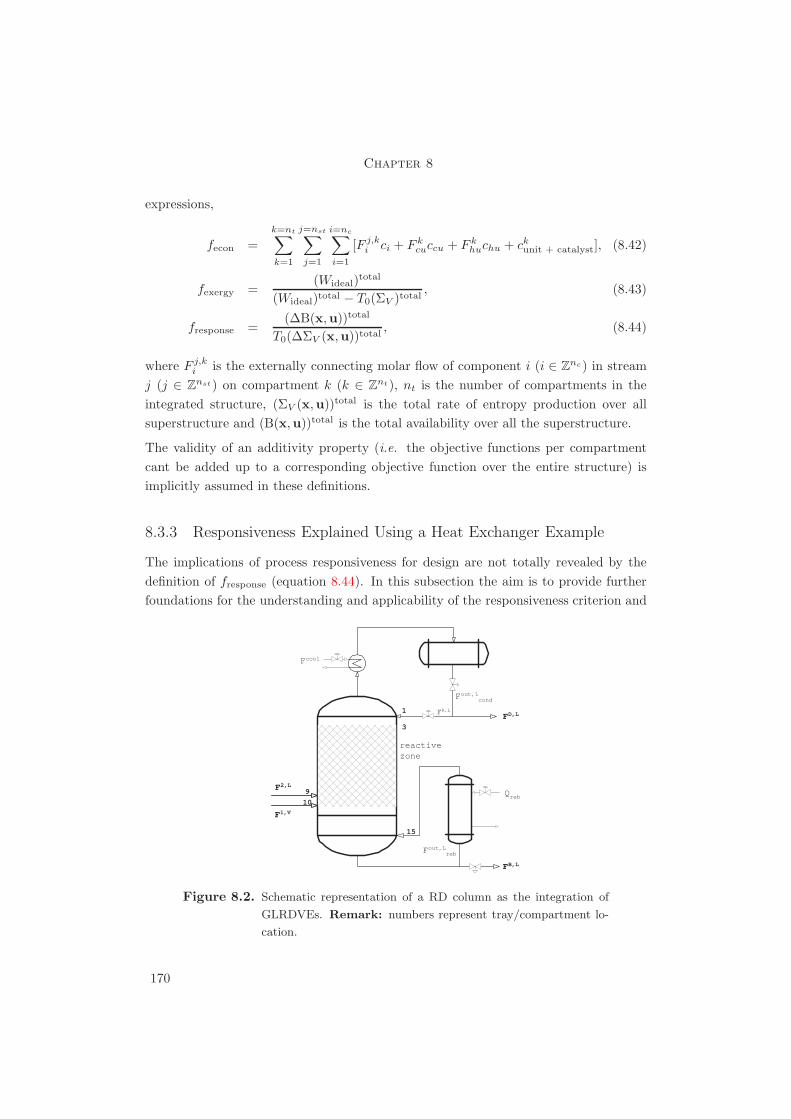
Chapter 8
expressions,
fecon =k=nt∑k=1
j=nst∑j=1
i=nc∑i=1
[F j,ki ci + F k
cuccu + F khuchu + ckunit + catalyst], (8.42)
fexergy =(Wideal)total
(Wideal)total − T0(ΣV )total, (8.43)
fresponse =(∆B(x,u))total
T0(∆ΣV (x,u))total, (8.44)
where F j,ki is the externally connecting molar flow of component i (i ∈ Znc) in stream
j (j ∈ Znst) on compartment k (k ∈ Znt), nt is the number of compartments in theintegrated structure, (ΣV (x,u))total is the total rate of entropy production over allsuperstructure and (B(x,u))total is the total availability over all the superstructure.
The validity of an additivity property (i.e. the objective functions per compartmentcant be added up to a corresponding objective function over the entire structure) isimplicitly assumed in these definitions.
8.3.3 Responsiveness Explained Using a Heat Exchanger Example
The implications of process responsiveness for design are not totally revealed by thedefinition of fresponse (equation 8.44). In this subsection the aim is to provide furtherfoundations for the understanding and applicability of the responsiveness criterion and
1
15
9
10
F2,L
������3
reactivezone
Fcool
Qreb
Fout,Lcond
Fout,Lreb
FR,LFD,L
F1,V
FB,L
Figure 8.2. Schematic representation of a RD column as the integration of
GLRDVEs. Remark: numbers represent tray/compartment lo-
cation.
170

A Design Approach Based on Irreversibility
its implications for design. An ideal heat exchanger is considered in this context as thecase study. The starting point of this analysis is directly derived from the definition offresponse. According to expression 8.44 a short responsiveness time is desired and can beattained by a large change in the entropy production rate for a given change in storedexergy.
8.3.3.1 System’s Features and Model Development
The following properties of the system are considered: (i) two liquid-phase streamsenter the heat exchange in a countercurrent set-up; (ii) the heat exchanger is operatedat isobaric conditions; (iii) both liquid streams are assumed behave ideally, (iv) bothstreams have equal physical properties, excluding heat capacity, which are tempera-ture independent; (v) heat transfer due to conduction is the only source of entropyproduction; and (vi) the driving force for heat transfer is computed between outletconditions.
The last assumption is driven by two practical motivations. Firstly, it allows a simpli-fied solution of the problem as no computations over all the unit’s length are required.Secondly, the situation under consideration is the milder one in terms of entropy pro-duced. At this condition the smallest thermal driving force is expected. If any effect onfresponse is registered, it may occur also with a magnified intensity at any other location.
Figure 8.3. Schematic representation of an ideal countercurrent heat ex-
changer to assess the responsiveness index.
According to the schematic representation in figure 8.3, both liquid-phase streams enterthe heat exchanger from opposite sides. Heat is transferred through the solid wallbetween the phases. The liquid holdup of each liquid is kept constant during theoperation so that inlet and outlet flows are equal. The set of governing equations andphysical properties of the system are given in tables 8.2 and 8.3, respectively. A degreeof freedom analysis is now performed to estimate the number of variables to be specifiedto consolidate the model. All variables of this system are grouped in a column vectorX, which contains 13 elements,
X ≡ [T in
i hini Fi Ti hi Q ∆Tlm A
]T. (8.45)
171

Chapter 8
The number of governing expressions as listed in table 8.2 equals 8. Out of the fiveremaining variables to be specified, three are considered fixed inputs and given by thevector I,
I ≡ [F1 T in
i
]T. (8.46)
Within the two remaining degrees of freedom, one is fixed by the design target (T1),leading to a single variable to be specified to consolidate the model. This variable couldbe either the outlet temperature of the cold utility or the heat transfer area. In thecourse of this subsection and to study the effect of varying thermal driving forces on theresponsiveness index, the area A is fixed. For the sake of comparison among differentunits, results for additional heat transfer areas are included.
8.3.3.2 Entropy Production Rate and Stored Exergy
The entropy of the system is assumed to be exclusively generated by the heat conduc-tion from the hot to the cold fluids. The entropy production rate, at microscopic level,can be estimated as the product of thermal driving force and heat flux. From a macro-scopic stand-point the measurable heat flow is used for this computation. A betterapproximation can be obtained by introducing phenomenological coefficients (Hasse,1969; Koeijer, 2002; Meeuse, 2003). For our analysis, however, we adopt an alterna-tive approach. The overall steady state entropy equation of change is applied and theproduction term is related to the net change of entropy.
Therefore, for this ideal system the entropy production rate is given by the overallcontributions of both streams,
∆Si = Cpi × lnTi
T ini
, i ∈ [1, 2], (8.47)
Table 8.2. Set of governing expressions for the ideal heat exchanger as de-
picted in figure 8.3. Remarks: stream 1 corresponds to the hot
utility, whereas stream 2 is the cold utility.
Balance Governing expression
Energy balance Q = F1 × (hin1 − h1)
Q = F2 × (h2 − hin2 )
Enthalpy definition hini = Cpi × (T in
i − T0)hi = Cpi × (Ti − T0)
Heat transfer Q = UHX × A× ∆Tlm
Temperature difference ∆Tlm = T in1 −T2−(T1−T in
2 )
log
(T in1 −T2
T1−T in2
)
172
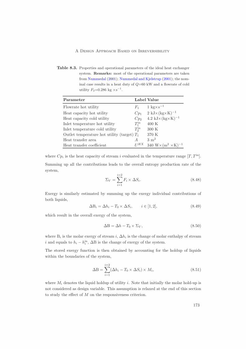
A Design Approach Based on Irreversibility
Table 8.3. Properties and operational parameters of the ideal heat exchanger
system. Remarks: most of the operational parameters are taken
from Nummedal (2001); Nummedal and Kjelstrup (2001); the nom-
inal case results in a heat duty of Q=60 kW and a flowrate of cold
utility F2=0.286 kg ×s−1.
Parameter Label Value
Flowrate hot utility F1 1 kg×s−1
Heat capacity hot utility Cp1 2 kJ×(kg×K)−1
Heat capacity cold utility Cp2 4.2 kJ×(kg×K)−1
Inlet temperature hot utility T in1 400 K
Inlet temperature cold utility T in2 300 K
Outlet temperature hot utility (target) T1 370 KHeat transfer area A 3 m2
Heat transfer coefficient UHX 340 W×(m2 ×K)−1
where Cpi is the heat capacity of stream i evaluated in the temperature range [T, T in].
Summing up all the contributions leads to the overall entropy production rate of thesystem,
ΣV =i=2∑i=1
Fi × ∆Si. (8.48)
Exergy is similarly estimated by summing up the exergy individual contributions ofboth liquids,
∆Bi = ∆hi − T0 × ∆Si, i ∈ [1, 2], (8.49)
which result in the overall exergy of the system,
∆B = ∆h− T0 × ΣV , (8.50)
where Bi is the molar exergy of stream i, ∆hi is the change of molar enthalpy of streami and equals to hi − hin
i , ∆B is the change of exergy of the system.
The stored exergy function is then obtained by accounting for the holdup of liquidswithin the boundaries of the system,
∆B =i=2∑i=1
(∆hi − T0 × ∆Si)×Mi, (8.51)
where Mi denotes the liquid holdup of utility i. Note that initially the molar hold-up isnot considered as design variable. This assumption is relaxed at the end of this sectionto study the effect of M on the responsiveness criterion.
173

Chapter 8
A disturbance scenario is considered to assess the response time function τ , where thetemperature target T1 changes +/- 10K around the nominal value,
T l1 < T1(t) < T u
1 , (8.52)
where the values of T l1 and T u
1 are 360K and 380K, respectively.
The driving force for heat conduction from the hot to the cold utility XHX is given bythe simplified expression,
XHX = ∆1T
=1T2
− 1T1. (8.53)
It is worth mentioning again that thermal driving force is computed between outletconditions. The motivation behind this assumption is given in section §8.3.3.1.
0 2 4 6 8 10 12 14 16 18 20 22 24 26 28 30230
240
250
260
270
280
290
Q=60 kW
Responsetime [s]
2.8
A=3.0 m 2
3.2
Thermal driving force [1/K*exp(-6)]
Figure 8.4. Response time as a function of the thermal driving force for an
idealized heat exchanger. Remarks: alternative designs with
different heat transfer areas are plotted and compared to the case
where Q=60 ·103 W (marker: �).
The values of response time τ as a function of the thermal driving force XHX arepresented in figure 8.4 and for designs of different heat transfer area A. Note that froma responsiveness stand point small driving forces are desired for a given heat exchangerdesign and the heat exchanger with the larger transfer area copes more efficiently withthe disturbance scenario. Summarizing, better process responsiveness is attained atsmaller driving forces (i.e. larger temperature difference and larger heat exchangers).
174

A Design Approach Based on Irreversibility
0 6 8 10 12 14 16 18 20 2205
100
150
200
250
300
350
400
450
500
550
M=50 mol
M=200 mol
M=100 mol
Responsetime [s]
Thermal driving force [1/K*exp(-6)]
Figure 8.5. Response time as a function of the thermal driving force for an ide-
alized heat exchanger at different hold-up values. Remarks: heat
transfer area: A=3 m2; heat duty of reference case: Q=60·103 W
(marker: �).
The effect of hold-up M on the responsiveness criterion is now analyzed. As suggestedby equation 8.51, smaller hold-up decreases the exergy storage and so helps to decreasethe time constant. This fact is depicted in figure 8.5, where hold-up values of 100 mol(reference value), 200 mol and 50 mol are used.
Based on the previous analysis the following practical heuristic can be suggested,
� Heuristic: maximize the exchange surface per unit of mass and keep driving forcesmall at constant transfer duty
8.3.4 Approach to Design Optimization and References Cases
At this point we have defined the superstructure of interest, developed three perfor-mance criteria for the optimization of the superstructure and provided some funda-mental insight into the impact of design variables on the responsiveness criterion. Inthis section the approach to solve the multiobjective optimization problem is presentedtogether with the reference design case to be compared with the optimized designs.
Two solving approaches are adopted to solve the optimization problem involving more
175

Chapter 8
Utopia point U in a RΦ-space is given by the Φ-objective functions values that solve independently
the Φ scalar optimization problems (Lim et al., 1999). For instance, in an optimization problem
involving two objective functions the mathematical formulation of the utopia point U is,
minx∈Γ
f1(x) = f l1(x∗), and f2(x∗) = fu
2 (x∗), (8.54)
minx∈Γ
f2(x) = f l2(x∗), and f1(x∗) = fu
1 (x∗), (8.55)
where f li and fu
i denote the lower and upper limits of the objective function fi, respectively; Γ
is the set of constraints, which define the space of design variables x.
The coordinates of the utopia point are then given by (f l1, f
l2). The meaning and optimization
potentiality of the utopia point is stressed using the following simple example. Let’s consider
the following multiobjective optimization problem,
Function: min(f1(x1, x2), f2(x1, x2)), (8.56)
s.t.: g(x1, x2) = 0, (8.57)
where
f1(x1, x2) = x1, (8.58)
f2(x1, x2) = x2, (8.59)
g(x1, x2) = x1 − x22 − 1 = 0. (8.60)
The solution of the optimization problem is depicted in a 2D plot of the involved objectives
(figure 8.6). Each non-inferior attainable optimal solution is estimated at a given combination of
objectives including constraint g(x1, x2). All these points define a curve of non-inferior solutions,
normally referred to as Pareto curve. For the sake of transparency a linear relation between
objectives is considered (i.e. F = Σwi × fi), where wi is the weighting factor of the objective
function fi and Σwi = 1. As expected, the utopia point is given by the coordinates
(f l1, f
l2) = (0,−50), (8.61)
which are the solutions of the scalar optimization problems.
Note 8.1. Utopia point in optimization problems with more than one objective
function
than one objective function,
• each objective function is used independently, disregarding the other two. Thisapproach localizes the coordinates of the utopia point and subsequently, reducesthe computational effort by limiting the search space. For a formal definition ofthe utopia point, the reader is referred to the explanatory note in table 8.1,
• the second approach accounts for the interactions and trade-offs among the objec-tives. Thus, a multiobjective problem is formulated by using a weighted p−normfor the vector of objective functions, as given by Clark and Westerberg (1983),
minD∈Γ
F ≡[∑
i
(wifi)p
] 1p
, p ∈ [1,∞), (8.62)
176

A Design Approach Based on Irreversibility
0 500 1000 1500 2000 2500−60
−50
−40
−30
−20
−10
0
f1 [−]
f2 [−]
f1l
f2l Pareto frontier
Region of attainable objectives
Utopia point
Figure 8.6. The role of utopia point in multiobjective optimization. Re-
marks: the optimization problem is formulated according to ex-
pression 8.56 given in the explanatory note of table 8.1; same note
provides the mathematical definition of the utopia point.
where F is the multiobjective function, w is a vector of weighting factors, f is thevector of objective functions, D is the set of decision variables and constrained bythe set Γ. According to Clark and Westerberg (1983) a norm of p ≤ 2 is used tolocalize non-inferior points in the non-convex regions.
This theory will now be applied to the multiobjective design cases for the MTBE col-umn. The reference design used for the sake of comparison is the structure previouslyintroduced in chapter 7. This structure corresponds to a reactive distillation column forthe synthesis of MTBE. The spatial design variables were obtained by steady-state op-timization of the unit’s economic performance. For background information, the readeris referred to section §6.2. The relevant parameters and schematic representation of theoptimized design are given in table 8.4 and figure 8.7, respectively.
177

Chapter 8
8.4 Application 1. Steady-state Entropy Production Pro-
file in a MTBE Reactive Distillation Column
The esterification of iC4 and methanol is used as the case study in this application. Adetailed description of the system is presented in appendix B. The chemical reaction isrepresented by a pseudo-homogeneous kinetics. The spatial configuration of the unit isthat obtained previously in section §6.2.
To prepare for the optimization task and to reduce the problem complexity we identifythe dominant contributions to entropy production rate over the MTBE column. Theexpressions to compute all contributions to the entropy production in the GLRDVEare summarized in table 8.5. In the case of a RD column structure these expressionsare applicable for all reactive and nonreactive compartments. Note that the reboilerand condenser models assume that the entropy contribution by external heat transferis dominant.
Table 8.4. Optimized design of a RD column for MTBE synthesis based on
economic performance. Remarks: information on this design
problem is given in section §6.2; bottom section lists the opera-
tional constraints and product specifications.
Value
Number of trays 15 [2:rectifying;8:reactive; 5:stripping]
Feed 1: location iC4+ nC4 : 10th tray (g)Feed 1: flowrate 455 mol×s−1
Feed 1: composition iC4 : 0.37; nC4 : 0.63Feed 1: temperature 350KFeed 2: location MeOH: 9th tray (l)Feed 2: flowrate 168 mol×s−1
Feed 2: composition MeOH: 1.00Feed 2: temperature 320KOperating pressure 11·105 Pa (top)Reflux ratio 7Mass of catalyst/tray 204.1 kg=1000 eq[H+]
Bottom flowrate 197 mol×s−1
Column diameter 7.132 mCondenser area 1.059·103 m2
Reboiler area 6.93·102 m2
Operational constraints P ≤ Pcond
Treb < Tc,iC4
Product specifications xDMTBE ≤ 0.1%xB
MTBE ≥ 99%
178

A Design Approach Based on Irreversibility
1
15
9
10
MeOH
C4-stream
���������
3
MTBE(>99%m)
MTBE(<0.1%m)
reactivezone
Fcool
Qreb
Fout,Lcond
Fout,Lreb
FR,L FD,L
Figure 8.7. Schematic representation of a RD column in the synthesis of
MTBE. Remarks: spatial design variables are listed in table
8.4; numbers represent tray location.
Table 8.5. Summary of expressions of all contributions to the entropy produc-
tion in a GLRDVE
Expression
mass transfer −i=nc∑i=1
Ji × aΨ × Xm,i
interface energy transfer JLq × aΨ × Xq +
i=nc∑i=1
Ji × aΨ × hi × Xe
chemical reaction 1T L
i=nrx∑i=1
ALi × εL
i × V LRX
external heat exchange Q× XHX
At this point the entropy profiles along the MTBE RD column due to the differentcontributions are estimated. These profiles are presented in figure 8.8 and correspondto the reference design as specified in table 8.4. The following results are of interest,
• the entropy profiles show that energy transfer contributes largely to the overallentropy production and particularly in the stripping section of the column, fol-lowed by mass diffusion. In the reactive zone, however, the dominant source ofentropy production is chemical reaction. In the rectifying section both mass and
179
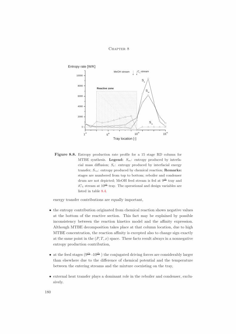
Chapter 8
0
2000
4000
6000
8000
10000
Reactive zone
MeOH stream C4-stream
15th10th5th1st
Entropy rate [W/K]
Se
Sm
Srx
Tray location [-]
Figure 8.8. Entropy production rate profile for a 15 stage RD column for
MTBE synthesis. Legend: Sm: entropy produced by interfa-
cial mass diffusion; Se: entropy produced by interfacial energy
transfer; Srx: entropy produced by chemical reaction; Remarks:
stages are numbered from top to bottom; reboiler and condenser
drum are not depicted; MeOH feed stream is fed at 9th tray and
iC4 stream at 10th tray. The operational and design variables are
listed in table 8.4.
energy transfer contributions are equally important,
• the entropy contribution originated from chemical reaction shows negative valuesat the bottom of the reactive section. This fact may be explained by possibleinconsistency between the reaction kinetics model and the affinity expression.Although MTBE decomposition takes place at that column location, due to highMTBE concentration, the reaction affinity is excepted also to change sign exactlyat the same point in the (P, T, x) space. These facts result always in a nonnegativeentropy production contribution,
• at the feed stages (9th -10th ) the conjugated driving forces are considerably largerthan elsewhere due to the difference of chemical potential and the temperaturebetween the entering streams and the mixture coexisting on the tray,
• external heat transfer plays a dominant role in the reboiler and condenser, exclu-sively.
180

A Design Approach Based on Irreversibility
In terms of entropy production, summarizing, the separation function dominates overthe reaction function for this MTBE RD column configuration.
8.5 Application 2. Bi-Objective Optimization of a MTBE Re-
active Distillation Column
A multiobjective optimization problem is formulated for the MTBE RD column withrespect to economic performance and exergy efficiency. The formulation includes thebalance equations 8.1-8.5 and 8.29, the criteria definitions 8.42 and the optimization for-mulation 8.62. Constraints imposed by operating conditions and product specificationsare included. For the sake of controlled built-up of optimization complexity the firstapproximation of this approach omits the response time constant as objective function.
The resulting optimization problem is formulated as follows and is implemented andsolved in gPROMS c©/gOPT c©,
minx∈Γ
J(fecon(x), fexergy(x), w), (8.63)
s.t. f(·) = 0,
h(·) ≤ 0,
where x denotes the set of design variables ([mcat Q aΨ])‡, f(·) is the set of algebraic ex-pressions that describe the system and h(·) is the set of inequalities defined by operatingconditions and product specifications (cf. bottom section of table 8.4).
The planar view of the two normalized objective functions at different weighting factorsis depicted in figure 8.9. The normalization of the objectives requires a priori knowledgeof the minimum (fmin) and maximum (fmax) values for each objective. These valuesare found by solving the optimization problem at different weighting factors. Eachobjective value is then scaled based on the corresponding utopia coordinate and fora given weighting factor Thus, the normalized objective functions (f ′) are computedaccording to the expression,
f ′i =
fi − fmini
fmaxi − fmin
i
, (8.64)
where the objective function fi is scaled with respect to the corresponding coordinatesof the utopia point,
f i =(wi × fi
fUi
)p
, i ∈ Zno , (8.65)
where no denotes the number of objective functions.
‡Operational variables such as reflux ratio and condenser pressure have been fixed to appropriate
reference values. Table 8.4 lists the actual values.
181

Chapter 8
0.0 0.2 0.4 0.6 0.8 1.00.0
0.2
0.4
0.6
0.8
1.0
f'econ
Q[0.5,0.5]
X[0,1]
E[1,0]
f'exergy
Figure 8.9. Pareto optimal curve fecon versus fexergy. Legend: E: economic-
based optimal design; X: exergy-based optimal design; Q: optimal
design based equally on economic performance and exergy effi-
ciency; Remarks: each point of the curve represents an optimal
solution in terms of the design variables [mcat, Q, aΨ] and weight-
ing factors w; axes are normalized so that utopia point coordi-
nates are: U=(0,0); original coordinates of U are: U0=(5.247·104
J×(s×K)−1,2.082 ·108 euro×y−1).
This curve is termed Pareto curve (cf. explanatory note 8.1) and clearly shows that oneobjective function can only be improved at the expense of the other objective function.This trade-off leads to significant deviations between optimal designs and the utopiapoint (up to 60%) for the pair f ′
econ − f ′exergy. The decision maker should have in mind
the importance of compromising both objectives at early stages of the design cycle.
Significant structural differences are noticed between the economic-driven (E; w =[1 0]T) and exergy-driven (X; w = [0 1]T) designs.
As depicted in figure 8.10, for instance, the catalyst load along the reactive trays differsamong the proposed designs when compared to the reference case (R†). The catalystload of the reference case is used to normalize the plot. When exergy is fully considered
†It is worth mentioning that, as expected, the optimal design based on economic performance (E)
coincides with the reference case (R).
182

A Design Approach Based on Irreversibility
3 4 5 6 7 8 9 100
1
2
3
4
5
6
E
X
Q
R
m'cat
[-]
Tray location [-]
Figure 8.10. Normalized catalyst distribution in the synthesis of MTBE with
respect to economic performance and exergy efficiency. Leg-
end: R: reference design, whose catalyst distribution is used
for normalization; E: optimal design based only on economic
performance; X: optimal design based only on exergy efficiency;
Q: optimal design based equally on economic performance and
exergy efficiency.
as an objective function the last reactive tray vanishes together with the sixth reactivetray. Furthermore, the catalyst load of the seventh reactive tray is considerably higherthan that of the nominal cases. This output suggest an alternative design, where aside reactor with high catalyst load is placed at the 7th tray. The catalyst load on theremaining reactive trays decreases when exergy is taken into account. The design withequally weighted objectives (Q; w = [0.5 0.5]T) presents an interesting catalyst loadprofile, specially at the 9th tray. The rather large catalyst load might be explained bythe reduced catalyst load on the last reactive tray and the constraint of targeting theproduct specifications. The reduced catalyst load on the 9th tray diminishes the MTBEdecomposition, at high MTBE composition and the product synthesis, at low MTBEcomposition. As a constraint in the product specification is included in the problemformulation, the required extent of reaction is accommodated only by having the 9th trayfully loaded with catalyst. Since MeOH is fed at the 9th tray, larger holdup of reactantis present and only converted into products by an increased amount of catalyst.
183

Chapter 8
0
1000
2000
3000
4000
5000
6000
7000
8000
15th10th
5th1st
Reactive zone
Srx
Sm
Se
Entropy rate [W/K]
Tray location [-]
Figure 8.11. Entropy production rate profile for an optimal design of a MTBE
RD column based on exergy efficiency (X-design). Legend:
Sm: entropy produced by interfacial mass diffusion; Se: entropy
produced by interfacial energy transfer; Srx: entropy produced
by chemical reaction; Remarks: stages are numbered from top
to bottom; MeOH feed stream is fed at 9th tray and iC4 stream
at 10th tray.
When the entropy profiles of the X-design (cf. figure 8.11) are compared with those ofthe E-design, it can be realized that the mayor contribution of entropy is still comingfrom the heat transfer process in the stripping section. However, mass diffusion becomesmore relevant than in the E-design. In the reactive zone and in contrast to the resultsof figure 8.8, the exergy by chemical reaction is unevenly produced along the reactivetrays. Thus, the 9th tray largely contributes to the overall exergy produced within thereactive section. A fully catalyst load on that tray intuitively explains this behavior.
According to these last results, it seems more attractive to reach high conversions onone or a few trays and low conversion on surrounding trays. Apparently, this findingseems to violate the equipartition principle of driving forces, under idealized conditions.Note that here we focus on the performance of RD process designs, paying less explicitattention to the industrial conventional processing route (see figure B.1). Therefore,a comparison between RD and non-RD processes with regard to entropy productionand the design implications for the principle of equipartition of forces are recommendedtopics to be further researched.
184

A Design Approach Based on Irreversibility
8.6 Application 3. Tri-Objective Optimization of a MTBE
Reactive Distillation Column: A Sensitivity-Based Ap-
proach
Based on the insight gathered in the previous applications, we are now ready to assessthe optimal design of a MTBE RD column with respect to fecon, fexergy and fresponse.For the sake of simplification, the following strategy is adopted: (i) an optimized designbased in economics and exergy efficiency is considered; (ii) a disturbance scenario isdefined; and (iii) the responsiveness index of the optimized design is estimated at thegiven disturbance scenario.
Optimized design. According to applications 1 (section §8.4) and 2 (section §8.5),the optimized designs based on fecon and fexergy present an important tradeoff betweenboth objectives. This tradeoff depends on the vector of weighting factors, w. Theultimate decision on w is made by the designer according to the requirements of thedesign problem. In our case and only for tutorial purposes, we choose the vector w =[0.3 0.7]T over all available designs. The optimized design variables for this case arelisted in table 8.6.
Disturbance scenario. The selection of a disturbance scenario is carried out byanalyzing qualitatively the entropy profiles of figures 8.8 (E-design) and (X-design)8.11 and by focussing on process disturbances occurring in industrial practice. Anupstream variation of the MeOH feed flowrate up to -10% is chosen as disturbancescenario.
FMeOH = FSSMeOH × (1 − ατ (t)), 0 ≤ ατ (t) ≤ 0.1, t ∈ [0, tf ]. (8.66)
Note that the disturbance scenario is chosen so that any steady-state transition isavoided. Further supporting arguments are given in section §7.3.2.
Responsiveness index. For each MeOH feed rate the variables B(x,u) and ΣV (x,u)are estimated in the corresponding steady state and the responsiveness index is com-puted. Note that the responsiveness index is treated as a function of the magnitude ofthe MeOH feed perturbation, fresponse(FMeOH).
Specifically, this MeOH flowrate disturbance results in a variation of the mass transferdriving forces for each component along the unit. From this point on, the analysisis focused on the top tray (1st), the 9th tray and the bottom tray (15th ) of the RDcolumn specified in table 8.6. Considering these tray locations, we provide a generalizedoverview on the unit’s responsiveness in the rectifying, reactive and stripping sections.The 9th tray is chosen because it is on that particular feeding tray where MeOH is fed tothe column and, therefore, where a more pronounced effect of feed flowrate disturbanceis expected. The corresponding mass transfer and chemical reaction driving forces are
185

Chapter 8
Table 8.6. Optimized design of a RD column for MTBE synthesis based
on economic performance and exergy efficiency. Remark: w =
[0.3 0.7]T.
Value
Number of trays 15 [2:rectifying;8:reactive; 5:stripping]
Feed 1: location iC4+ nC4 : 10th tray (g)Feed 1: flowrate 455 mol×s−1
Feed 1: composition iC4 : 0.37; nC4 : 0.63Feed 1: temperature 350KFeed 2: location MeOH: 9th tray (l)Feed 2: flowrate 168 mol×s−1
Feed 2: composition MeOH: 1.00Feed 2: temperature 320KOperating pressure 11·105 Pa (top)Reflux ratio 7Mass of catalyst [eq[H+]] m1:2=0; m3=771.9
m4=826.122; m5=762.405m6=688.412; m7=652.292m8=785.991; m9=1359.42m10=982.448; m11:15=0
Bottom flowrate 197 mol×s−1
Column diameter rectifying: 6.95 mreactive: 6.95 mstripping: 6.33 m
Condenser area 1.059·103 m2
Reboiler area 6.93·102 m2
plotted for trays 1, 15 and 9 in figure 8.12. It can be seen from these plots that bothMeOH mass transfer driving forces increase with larger disturbances, whereas chemicalreaction driving force decreases.
The response time of the MTBE RD column as a function of Xi,MeOH (1st and 15th tray)and Xrx (9th tray) is depicted in figure 8.13. The variation of B(x,u) and ΣV (x,u)are computed between the initial reference state and between consecutive states. Notethat the response time becomes larger at small Xi,MeOH-values in the rectifying andstripping sections, whereas small driving forces lead to short response times in thereactive section. From a responsiveness perspective, therefore, small driving forcesare desirable for reactive sections and large driving forces are desirable for separation(nonreactive) sections.
The first statement suggests that in the case of reactive sections driving forces shouldbe manipulated to control the unit while flux is specified (i.e. a certain conversion rate).
186

A Design Approach Based on Irreversibility
0 2 4 6 8 10 12
7.5
8.0
8.5
168 164.6 161.2 157.8 154.4 151 147.6
MeOH feed flowrate [mol/s]
reference steadystate
MeO
H m
ass
tran
sfer
driv
ing
forc
e [J
/mol
/K]
Variation of MeOH feed flowrate [%]
(a) Rectifying section, 1st tray.
0 2 4 6 8 10 1211.84
11.85
11.86
11.87
11.88
11.89
11.90
11.91
168 164.6 161.2 157.8 154.4 151 147.6
reference steadystate
MeOH feed flowrate [mol/s]
MeO
H m
ass
tran
sfer
driv
ing
forc
e [J
/mol
/K]
Variation of MeOH feed flowrate [%]
(b) Stripping section, 15th tray.
0 2 4 6 8 10 12
62.0
62.5
63.0
63.5
64.0168 164.6 161.2 157.8 154.4 151 147.6
reference steadystate
MeOH feed flowrate [mol/s]
Rea
ctio
n dr
ivin
g fo
rce
[J/m
ol/K
]
Variation of MeOH feed flowrate [%]
(c) Reactive section, 9th tray.
Figure 8.12. Driving forces as a function of the MeOH feed flowrate. Re-
marks: MeOH feed flowrate varies from the nominal value (168
mol ×s−1) to 150 mol ×s−1; the optimal design variables and
sizing parameters corresponds to a fecon − fexergy design, with
w = [0.3 0.7]T.
Explaining this requires the introduction of an approximated relation between fluxesand forces (Luyben et al., 1999; Hasse, 1969),
Jk ≈ α× Xk, (8.67)
T0 × ∆ΣV ≈ 2× T0
∫V
dV∑
k
α× Xk × ∆Xk, (8.68)
where α is a design factor, called thermodynamic design factor by Meeuse (2003).
At small gradient X the design factor α should be large enough to obtain the requiredflux. In the reactive section small reaction driving forces requires a large reaction volumeon the tray. Small variations in the MeOH feed flowrate produce large changes in theaffinity and subsequently large entropy production rate values. As the stored exergy
187

Chapter 8
7.8 7.9 8.0 8.1 8.2 8.3 8.4 8.5 8.6 8.7
100
1000
10000
difference betweenreference state
difference betweenconsecutive states
Responsetime [s]
MeOH mass transfer driving force [J/mol/K]
(a) Rectifying section, 1st tray.
11.870 11.875 11.880 11.885 11.890 11.895 11.900 11.905 11.910
100
1000
10000
difference betweenreference state
difference betweenconsecutive states
Responsetime [s]
MeOH mass transfer driving force [J/mol/K]
(b) Stripping section, 15th tray.
61.8 62.0 62.2 62.4 62.6 62.8 63.0 63.2
100
1000
10000
difference betweenreference state
difference betweenconsecutive states
Response time [s]
Reaction driving force [J/mol/K]
(c) Reactive section, 9th tray.
Figure 8.13. Response time as a function of the MeOH feed flowrate. Re-
marks: MeOH feed flowrate varies from the nominal value (168
mol ×s−1) to 150 mol ×s−1; the optimal design variables and
sizing parameters corresponds to a fecon − fexergy design, with
w = [0.3 0.7]T.
changes only modestly with a small flow disturbance, the overall effect enhances theprocess responsiveness (i.e. small response times).
The second statement can be explained by following the same reasoning. In a distillation(separation) process the driving force (top-bottom) is specified and the flux remains toinfluence. Thus, in nonreactive sections flux should be manipulated to control the unit.The results of these observations fully agrees with the analysis given by Luyben et al.(1999) and Meeuse (2003) for a reactor and distillation column.
Meaningfulness and validity of results. Note that in the current approach acontinuous range of disturbances for one input variable is considered for the computationof the responsiveness time constant. In comparison with the generalized definition of
188
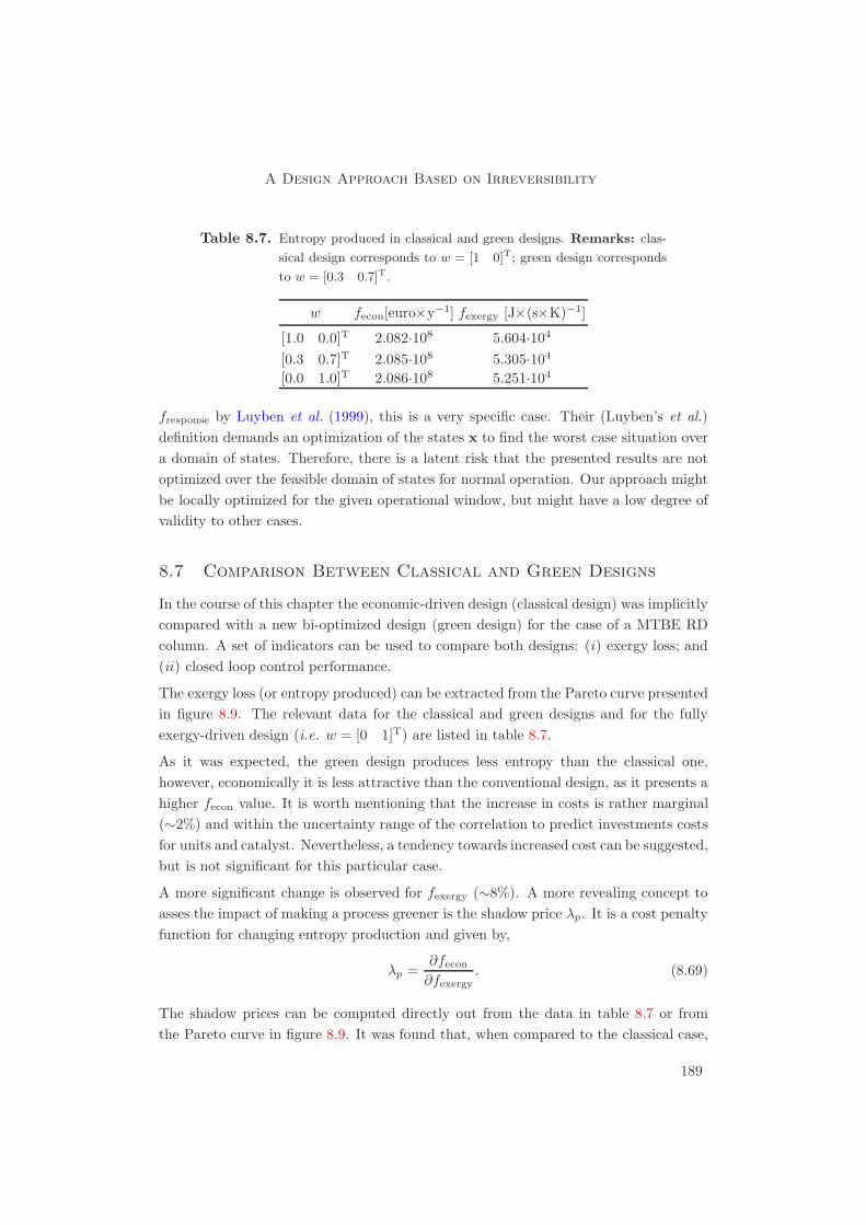
A Design Approach Based on Irreversibility
Table 8.7. Entropy produced in classical and green designs. Remarks: clas-
sical design corresponds to w = [1 0]T; green design corresponds
to w = [0.3 0.7]T.
w fecon[euro×y−1] fexergy [J×(s×K)−1]
[1.0 0.0]T 2.082·108 5.604·104
[0.3 0.7]T 2.085·108 5.305·104
[0.0 1.0]T 2.086·108 5.251·104
fresponse by Luyben et al. (1999), this is a very specific case. Their (Luyben’s et al.)definition demands an optimization of the states x to find the worst case situation overa domain of states. Therefore, there is a latent risk that the presented results are notoptimized over the feasible domain of states for normal operation. Our approach mightbe locally optimized for the given operational window, but might have a low degree ofvalidity to other cases.
8.7 Comparison Between Classical and Green Designs
In the course of this chapter the economic-driven design (classical design) was implicitlycompared with a new bi-optimized design (green design) for the case of a MTBE RDcolumn. A set of indicators can be used to compare both designs: (i) exergy loss; and(ii) closed loop control performance.
The exergy loss (or entropy produced) can be extracted from the Pareto curve presentedin figure 8.9. The relevant data for the classical and green designs and for the fullyexergy-driven design (i.e. w = [0 1]T) are listed in table 8.7.
As it was expected, the green design produces less entropy than the classical one,however, economically it is less attractive than the conventional design, as it presents ahigher fecon value. It is worth mentioning that the increase in costs is rather marginal(∼2%) and within the uncertainty range of the correlation to predict investments costsfor units and catalyst. Nevertheless, a tendency towards increased cost can be suggested,but is not significant for this particular case.
A more significant change is observed for fexergy (∼8%). A more revealing concept toasses the impact of making a process greener is the shadow price λp. It is a cost penaltyfunction for changing entropy production and given by,
λp =∂fecon∂fexergy
. (8.69)
The shadow prices can be computed directly out from the data in table 8.7 or fromthe Pareto curve in figure 8.9. It was found that, when compared to the classical case,
189

Chapter 8
0 10000 20000 30000 40000 50000 600000.9960
0.9965
0.9970
0.9975
0.9980
0.9985
Bi-optimized design(green)
Economic-driven design(classical)
xMTBE
[-]
Time [s]
Figure 8.14. Time variation of MTBE product stream for the classic and
green designs in the presence of a MeOH feed flowrate distur-
bance. Remarks: green design corresponds to w = [0.3 0.7]T;
column specifications for classic and green designs are given in
tables 8.4 and 8.6, respectively.
the green design presents a cost penalty of ∼ -2.02, whereas the X-design a value of∼ -4.37 [euro ×K ×MJ−1]. These values confirm the trade-off between both objectivesand suggest that the greener the design the larger the involved cost penalty.
The closed loop control performance of both designs is now analyzed. The disturbancescenario under consideration is the one used previously in section §7.3. Thus, a stepvariation in the flowrate of methanol during the time horizon of 6·104 s is given by,
FMeOH =
F
SSMeOH if t < 1 · 104 s or t > 4 · 104 s,
1.1× FSSMeOH if 4 · 104 s > t > 1 · 104 s.
(8.70)
The dynamic response of the classic and green designs are depicted in figure 8.14. In thisfigure the MTBE composition at the bottom stream is presented as a function of timein the presence of the MeOH feed disturbance. Note that the bi-optimized design (i.e.green) has an improved closed loop performance compared with the classical design.The deviation from xMTBE set-point are less pronounced in the green design, whichsmoothly returns back to the initial steady state when the disturbance disappears.Note that the set-point of the green design is slightly lower (0.05%) than the one ofthe classic design. This negligible variation in set-points does not affect the quality of
190

A Design Approach Based on Irreversibility
the analysis results. It is suggested from our results that incorporating both economicand exergy-related objectives in the unit design results in a process with better closedloop performance, provided that control structure and tuning are kept invariant. It isworth clarifying that a well-tuned control can compensate for any change in the processoperability feature.
8.8 Concluding Remarks
The starting point of this chapter was the definition of a generic building block forprocess synthesis (GLRDVE). The sources and the distribution of the entropy produc-tion rate in a complete MTBE column were then determined and analyzed. It is be-lieved that insight into such a distribution is helpful for assessing which column relateddesign decision variables (e.g. feed tray location, reflux ratio, heat load distributionusing diabatic operation, catalyst load and mass/heat transfer area) are key to opti-mize the column performance. The perspective adopted for selecting the design decisionvariables was task-oriented rather than the conventionally used equipment-oriented de-sign approach. The chosen design decision variables included the reaction volume, theamount of heat to be added or removed and the interfacial areas for species mass andheat transfer. Operational variables such as reflux ratio and condenser pressure werefixed at appropriate reference values. Analyzing the steady state entropy productionprofiles in a MTBE RD column showed that, in terms of entropy production, the sepa-ration function dominates over the reaction function. A bi-objective function was thenstudied regarding economic and exergy performance. It is suggested that designs basedexclusively on economic or exergy performances differ significantly in their structure,showing an existing trade-off. The Pareto curve provides sensitivity information on thecost effects of improving the exergy efficiency. In addition to economics and exergyobjectives, this optimization-based approach covers responsiveness aspects. To definea responsiveness criteria, the availability and entropy production rate are regarded asfunctions of an internal state vector x and a vector of disturbances and/or manipulatedexternal excitations u. In our approach the maximization approach suggested by Luy-ben et al. (1999) is not considered due to its inherent need for high computational effort.However, a rather formal definition of fresponse was adopted together with a single inputexcitation. Note that by not searching over all possible state trajectories, the generalityof the results might be questionable and the external excitation is a fairly conservativeone. Analyzing the responsiveness criteria of the bi-optimized design it reconfirmedthat small driving forces are desirable for reactive sections and large driving forces aredesirable for separation (nonreactive) sections (Luyben et al., 1999; Meeuse, 2003). Thefirst statement suggests that, in the case of reactive sections, driving forces should bemanipulated to control the unit. The second statement suggests that in nonreactive
191

Chapter 8
sections flux should be manipulated to control the unit. Finally, the economic-drivendesign (classical design) was compared with the new bi-optimized design (green design)for the case of the MTBE RD column. The green design produces less entropy than theclassical one, while being economically less attractive (marginal). The bi-optimized de-sign has an improved closed loop performance compared to the classical design, keepingthe same control structure and settings. It is concluded that incorporating both eco-nomic and exergy-related objectives in the unit design results in a process with betterclosed loop performance and reduced exergy loss.
Mind journey to the scientific questions.
In this chapter three performance criteria were introduced in theRD design problem derived from a life-span perspective. The in-corporation of those performance criteria resulted in designs withstructural differences and with balanced economic-performance,thermodynamic efficiency and that are capable of coping with arealistic disturbance scenario. Thus, the material presented inthis chapter effectively answers Question 7.
192

“It is through science that we prove, but through intuition
that we discover.”
Henri Poincare, mathematician (1854-1912)
9Conclusions and Outlook
This dissertation covers the design of grassroots reactive distillation processes. In this
concluding chapter we attempt to highlight the key contributions of this research to
the scientific knowledge domain of reactive distillation process design. Here we pay
special attention to the answers of the goal-oriented and engineering questions posted
at the end of chapter 1. Additionally, we discuss various paths for further research
and give some recommendations for future endeavors.
193

Chapter 9
9.1 Introduction
The design and operation of reactive distillation processes has received increasing atten-tion within academia and industrial spheres over the last decades (cf. figure 1 in Maloneand Doherty (2000)). From a process intensified perspective and because of its inherentcomplexity, addressing RD is a challenging task. In the course of this dissertation wehave present the relevant results and approach that can be used to produce a life-spaninspired design for reactive distillation processes. In this regard, after having coveredthe fundamentals of RD and current design approaches (chapters 2 and 3), we suggesta novel methodology for RD process design (chapter 4), which then becomes the focusof chapters 5-8. Each chapter covers a specific aspect of the LiSp-IDM, i.e. life-spaninspired design methodology) and answers to the engineering questions (questions 4-7)posted in chapter 1 are provided. Taking a broader perspective these engineering an-swers will now be used to address the goal-oriented questions (questions 1-3), eitherqualitatively or quantitatively.
This chapter is organized as follows: in section §9.2 we recall the specific design questionsand provide the supporting scientific argumentation for the answers. In section §9.3, weinfer the answers to the goal-oriented engineering questions. We adopted this orderingbased on the assumption that the material presented in the previous chapters remainsin the reader’s memory, or at least it is easily retrieved. We address the novelty aspectsof this research in section §9.4. The open opportunities identified in the course of thiswork are discussed along with recommendations for further research in section §9.5.
9.2 Conclusions Regarding Specific Scientific Design Ques-
tions
Recalling the specific scientific design questions formulated at the beginning of this the-sis, we can draw the following conclusions.
Question 4. What is the domain knowledge required and which new echelonsare needed for process synthesis?
� Answer. Temporal domain knowledge, physical and operational knowledge andspatial-related knowledge; a multiechelon approach: formulation, feasibility analysis,temporal structure, generation of separation sequences, internal spatial structure, be-havior analysis, evaluation.In the case of RD, the design issues are far more complex than those relating to conven-tional distillation and they may differ significantly from case to case. Thus, we suggestthat the domain knowledge required for any (integrated) design methodology shouldbe classified into three key areas: (i) temporal considerations, (ii) physical and opera-
194

Conclusions and Outlook
tional conditions and (iii) spatial parameters. In terms of priority of decision the firstclass of key design decision variables involves temporal considerations. The variables ofinterest relate to the mode of operation of the system, namely batch, fed batch or con-tinuous operation, together with the time horizon. The second class of design variablesincludes the physical and operational conditions of the system. These are aimed at thefavorable creation of enough reaction and separation driving forces and mutual synergy.In this class design variables such as operation pressure, temperature, reflux ratio andphase velocity are of utmost importance. Moreover, the chemical reaction regime andmass/heat transfer regime should be specified. The third and last class of decision classembraces all key spatial parameters, ranging from establishing section with differentfunctionalities, packing parameters, number of trays or length of sections, feeding andwithdrawal points, energy exchange, section diameters, column flowsheet configurationwith recycle structures and heat integration.
Both graphical and optimization-based design methods have already shown proven po-tential in RD process design, but some significant limitations have also been found.Graphical methods are fairly flexible for generating alternative designs at various de-sign parameters, allowing the designer to define realistic bounds. Furthermore, thegraphical nature of the methods helps us to clarify our understanding of these funda-mental issues in RD, which might be disguised by other approaches. However, graphicalmethods are strongly limited by their graphical nature.
Optimization-based methods overcome this last limitation and can be used to solvesuccessfully design problems that involve multicomponent mixtures, multiple chemicalreactions and multiple units. However, additional caution is required during problemformulation and inappropriate initial guesses made for the optimization variables maylead to convergence difficulties. Evolutionary methods are used to cover, in more detail,some of the physical aspects of the design of RD columns. However, this approachrequires a pre-defined structure and accordingly, an optimum design is not guaranteed.
Due to the size and conceptual/computational complexity of the RD design problem, asingle comprehensive design strategy might not be available for some years to come. Inthis research, however, we propose an integrated design approach, termed multiechelondesign approach. This strategy allows the designer to combine, in a systematic way, thecapabilities and complementary strengths of the available graphical and optimization-based methods. Decomposition to give a hierarchy of imbedded design spaces of increas-ing refinement is used to support this approach. Moreover, it constitutes the frameworkof a highly aggregated design methodology, which focuses on the RD design problemfrom a life-span perspective (LiSp-IDM in chapter 4). The following building blocksconstitute the body of the multiechelon design approach:
Formulation. Sustainability issue are considered and the basis of design are defined,
195

Chapter 9
i.e. product and feedstock purities ranges, production modes, operating window andeconomics, and appropriate building model blocks are developed (e.g. thermodynamic,kinetic and hydrodynamic).
Feasibility analysis. Using graphical methods the feasible product compositions fora given set of input variables are determined (e.g. feed composition and Damkohlernumber) incorporating all occurring phenomena (e.g. distillation boundaries, (non)-reactive azeotropy).
Temporal structure. The operation mode is selected, i.e. batch, continuous or semi-batch, based on operational skills, production requirements and supply chain dynamics.
Generation of separation sequences. The use of rigorous graphical methods allowsus to identify and organize feasible column sequences. It is necessary to estimate theirtype of task, i.e. fully reactive, hybrid and nonreactive columns, together with thenumber of units and their connectivity.
Internal spatial structure. The process structure obtained from the previous levelis used as starting point for this stage. Using optimization-based methods we canobtain continuous variables (e.g. column diameter, heat exchange areas, contactingarea, catalyst concentration, reboil and reflux ratios) and discrete variables (e.g. feedstaging, reactive and nonreactive stages, withdrawal staging).
Behavior analysis. Steady-state simulations are used to explore the kinetics, G/Lmass transfer, hydrodynamics and multiplicities inside the units. Additionally, dynamicsimulations are performed to check the robustness of the design, in terms of the abilityto maintain product purities and conversion within a desired range when disturbancesoccur.
Evaluation. The design options are checked with respect to their performance. Takingthe wide range of criteria in the safety, health, economics, environment and technology(SHEET) aspects specific choices are made for economic performance, sustainability andtechnology. With respect to economics, we calculate the capital and operational costsof a process for its time horizon. We use exergy efficiency as a sustainability metric,while a systems response time is used to define the responsiveness of the process.
Question 5. What are the (performance) criteria that need to be consideredfrom a life-span perspective when specifying a reactive distillation designproblem?
� Answer. Safety, health, environment, economics and technology (SHEET)-relatedmetrics; in particular TAC, entropy production rate and response time.Aiming at a design methodology that addresses the problem from a life-span perspective,we suggested a set of performance criteria. The motivation behind our perspective relies
196

Conclusions and Outlook
on the relevance of economic performance and potential losses over the process life span.Specifically, we took into consideration exergy-efficiency and responsiveness issues.
We considered a set of criteria embracing issues related to safety, health, environment,economics and technology (SHEET). Provided that safety and health issues are inherentin a responsible design approach, the remaining issues can be used to define a novel per-formance space. Environmental considerations are directly linked to the minimizationof mass, energy and exergy losses. Economic performance is translated quantitativelyto the capital and operational costs of the design. We used the total annualized cost(TAC) as a convenient index. Additionally, we considered exergy efficiency to be anenvironment-based metric, more specifically the entropy production rate. We completedthe performance criteria set by appending a technology-based index. In this work wesuggested that the responsiveness of the process can be used as an adequate metric andmore specifically the response time as defined in Luyben et al. (1999). Using this metricwe get a measure for prevention of loss of material and energy.
Question 6. What (new) methods and tools are needed for reactive distilla-tion process synthesis, analysis and evaluation?
� Answer. Improved residue curve mapping technique, multilevel modeling approach,dynamic optimization of spatial and control structures, steady-state and dynamic be-havior analysis, generic lumped reactive distillation volume element, multiobjective op-timization criteria.In the course of this thesis we have covered novel tools and methods that can be usedto assist the design of reactive distillation processes (see chapters 5 to 7). A briefdescription of the highlights of the chapters is given below.
We showed that residue curve maps provide valuable insights and design assistancefor nonideal systems, particularly for RD. Transforming the composition variables ac-cording to Doherty’s approach allows us to define a reaction invariant space of lowerdimension, formed by attainable product compositions and where the conventional con-cepts for residue curves can be applied. For the MTBE synthesis we defined two mainsubregions in the modified composition simplex, each of which were characterized bysingular points and delimited by separation boundaries. We generated two differentseparation sequences, covering all the possible reacting mixture compositions.
We proposed a multilevel modeling approach, regarded as an easy-to-handle tool in theearly stages of design. We derived two model levels of different degree of complexity tomodel the processes taking place in a RD column. Additionally, we performed rigorousand reliable degree of freedom analysis at each level, where appropriate business-relateddecision variables are included. These levels involve an outer (input-output) view andan inner (physical task) view. These models are linked by the extent of reaction vector,
197

Chapter 9
which allows us to establish whether or not the models are well specified and mutuallyconsistent. Additionally, the approach allows one to determine whether or not thebusiness-related decision variables cope with the operational constraints imposed by theproblem formulation (e.g. the SHE issues, reactants availability and market demand).
Formulating design as a dynamic optimization problem, we found that for the synthesisof MTBE, a tradeoff between control and economic performances exists. We solvedthis multiobjective optimization problem by incorporating appropriate time-invariantparameters (e.g. column diameter, heat transfer areas and controllers’ parameters) inthe frame of a dynamic optimization problem in the presence of deterministic distur-bances. The design optimized sequentially with respect to dynamic behavior leads to aRD process with a total annualized cost higher than that obtained using simultaneousoptimization of spatial and control structures.
The nonlinear coupling of reactions, transport phenomena, phase equilibria and hard-ware hydraulics arises as a result of the highly complicated dynamic behavior of thesystem. We showed that, even for a simplified reactive flash and an idealized system,a large number of bifurcation diagrams could be identified. We suggest that the mainsource of multiplicity is the strong nonlinear coupling of reactions, transport phenomenaand phase equilibria. We used singularity to study the steady-state behavior in RD,with a particular focus on a reactive flash with a rather ideal system undergoing a mildlyexothermic isomerization reaction using a light-boiling reactant. For this case the num-ber and relative location of the turning points and feasibility boundaries correspondingto no-liquid or no-vapor products determined the qualitative nature of the bifurcationdiagram. State multiplicity is present in a large area of the parameter space, for thecase under consideration. We identified a large number (25) of qualitatively differentbifurcation diagrams for the system. The feasibility boundaries played an importantrole in the classification of the reactive flash. Up to five feasibility boundaries and amaximum of 3 steady states were found in a single bifurcation diagram. Bifurcation di-agrams exhibiting more then two feasibility boundaries are common for liquid or vaporfeed. Increasing the heat of reaction, activation energy or relative volatility enlargesthe area of multiplicity. Furthermore, a large heat of reaction can create regions inparameter space with 5 feasibility boundaries in a single bifurcation diagram.
Moreover, we explored the process dynamics of a full RD unit using a rather conventionalapproach. The scope of this analysis was restricted to a limited version of control systemdesign, as a single input-single output structure and proportional-integral controllerswere selected a priori selected. The outcome of this approach was used to set a referenceperformance for the next novel contribution involving the trade-off between design,responsiveness and sustainability aspects. We developed a generic dynamic model fora complete RD column. This model is composed of instances of (non-) reactive trays,condenser, reflux drum, reboiler and controllers. Based on a rigorous degree of freedom
198

Conclusions and Outlook
analysis and some engineering judgment a control structure was defined. Using thesynthesis of MTBE as our case study, we simulated dynamically the unit behavior inthe presence of realistic disturbances scenarios. Using comparison with published work,we found a satisfactory degree of agreement between our unit output and literaturedata. Moreover, our proposed control structure led to minor variations in the MTBEbottom fraction in the presence of disturbances.
Question 7. Are there structural differences and significant improvements indesigns derived using conventional methodologies from those obtained usingan integrated design methodology?
� Answer. Reduction in the number of reactive trays, more uneven distribution ofcatalyst and identification of suitable spots for side reactors.We defined a generic building block for process synthesis: the generic lumped reactivedistillation volume element. We then determined and analyzed the sources and distrib-ution of the entropy production rate in a complete MTBE column. We strongly believethat insight into such a distribution is helpful for assessing which column related designdecision variables are key to optimize column performance. The perspective adopted forselecting the design decision variables was task-oriented rather than the conventionallyused equipment-oriented design approach. Analyzing the steady state entropy produc-tion profiles in a MTBE RD column we found that, in terms of entropy production,the separation function dominates over the reaction function. Afterwards, we studieda bi-objective function with respect to economic and exergy performance. We foundthat designs based on economic or exergy performances differed significantly in theirstructure, showing an existing trade-off. For instance, the catalyst load along the reac-tive trays differed among bi-optimized designs (‘green’) when compared to the reference‘conventional’ case. Hence, the number of reactive trays and catalyst load diminisheswhen exergy is optimized. Trays with high catalyst loading could be candidate spots forplacing a side reactor. In addition to the economics and exergy objectives, we analyzedresponsiveness aspects in this optimization-based approach. To define a responsivenesscriterion we adopted a rather specific definition of response time, it being the change inavailability over the change in entropy production rate due to a single input excitation.Analyzing the responsiveness criteria of the bi-optimized design we reconfirmed thatsmall driving forces are desirable for reactive sections and large driving forces are de-sirable for separation (nonreactive) sections. Finally, we compared the economic-drivendesign (classical design) with the green design for the case of the MTBE RD column.We found that the green design produced less entropy than the classical one, while beingmarginally less attractive from an economics standpoint. Moreover, the green designhad an improved closed loop performance compared to the classical design, keepingthe same control structure and settings. We concluded that incorporating both eco-
199
Chapter 9
nomic and exergy-related objectives in the unit design results in a process with betterclosed loop performance and reduced exergy loss for this specific case study. These factsprovided the motivation for our life-span inspired perspective.
9.3 Conclusions Regarding Goal-Oriented Questions
After having addressed the engineering specific questions we propose the following an-swers to the goal-oriented questions.
Question 1. What benefits can be gained from having a more integrateddesign methodology?
In this thesis we proposed and addressed, at a certain degree of detail, a life-span in-spired design methodology (LiSp-IDM, see chapter 4). The framework of our approachwas derived from an extensive analysis of current design methodologies in RD. Thus,the suggested multiechelon approach combines, in a systematic way, the capabilitiesand complementary strengths of the available graphical and optimization-based designmethodologies. The multiechelon approach is also supported by decomposition to givea hierarchy of imbedded design spaces of increasing refinement. As a design progressesthe level of design resolution can be increased, while constraints on the physical feasi-bility of structures and operating conditions derived from first principles analysis canbe propagated to limit the searches in the expanded design space.
The benefits of adopting such an integrated methodology are of different nature, rang-ing from responsible use of resources (via minimization of entropy production rate),economical attractiveness (via minimization of total annualized costs) and improvedprocess responsiveness (via minimization of response time metric). Using gradual re-finement of the design spaces we introduced a beneficial understanding of the ongoingphysical and chemical phenomena and guaranteed a more efficient conceptual designwith respect to the SHEET criteria.
The successful application of the integrated design methodology relies on consider-ing the output of the graphical methods as an initial structure on which to base theoptimization-driven design approaches. In this way, the optimized design is likely tobe embedded within the feasible space and the computational effort becomes less de-manding due to the reduced number of design variables. This approach is intendedas a means to decompose the complexity of the design problem and it should not beconsidered as a mechanistic recipe.
200

Conclusions and Outlook
Question 2. What are the practical constraints that need to be consideredfrom a resources point of view, i.e. time, costs, tools and skill levels, whendeveloping and applying a design methodology in a work process?
The design task is often regarded as a difficult to master activity, due to the highnumber of design decision variables and combinatorial complexity. For the RD case thisaspect is magnified due to the large number of additional design variables that haveto be considered and the presence of more interacting phenomena, when compared toconventional nonreactive separation.
This research has shown that the integrated design methodology, more specifically themultiechelon design approach, while it is a way to beat design complexity by decompo-sition, requires the mastery of many tools (e.g. RCM, MINLP and rigorous dynamicmodeling) and many concepts (e.g. bifurcation, singulary theory and dynamic optimiza-tion). A schematic representation of the tools and concepts required for each designechelon is given in figure 9.1. This amazing complexity means that the required skilllevel is even higher than was initially assumed.
Question 3. What are the essential ingredients for such a design methodol-ogy?
Our integrated design methodology is composed of various design spaces, as describedin chapter 4. These design spaces are the essential ingredients for a life-span approachand are characterized by the flow of information and knowledge domain. In the courseof this thesis, we have addressed each space and, moreover, we have discussed theinput-output information flow. These information aspects and the knowledge domainsinvolved in each design space are summarized in table 9.1. Each design space (orechelon) is supported by a tool-kit, which includes techniques and concepts such asRCM, MINLP, dynamic modeling, dynamic optimization, irreversible thermodynamics-based and singularity theory.
9.4 Scientific Novelty of this Work
In this dissertation we addressed the fundamentals of reactive distillation process designand attempt to generate scientific novelty. These contributions to the knowledge domainare grouped in the following categories.
Formulation of an extended design problem. We formulated a refreshed andmore comprehensive RD design problem in the wider context of process developmentand engineering and in a more relevant way regarding sustainability. The nature ofthe extension is given by the identification of the design decision variables and theirgrouping into three categories: (i) those related to temporal considerations; (ii) those
201

Chapter 9
Feasibility analysis
Generation of separation sequences
Internal spatial structure
Behavior analysis
Evaluation
RCM
RCM
dynamic optimization,rigorous modeling,MINLP
singularity theory,dynamic optimization
irreversible thermodynamics,multiobjectiveoptimization
DESIGN SPACE (echelon) TOOLS
Figure 9.1. Schematic representation of the tools and concepts required at
each design echelon
202

Conclusions and Outlook
Table 9.1. Summary of input-output information flow
Design specifications Design/operational variables Domain knowledge
Feasibility analysis
Process: Discrete: - thermodynamics
- set of components - distillation boundaries - kinetics
- set of chemical reactions - (non-) reactive azeotropes - overall balances
- feed composition Continuous:
- operational pressure - product feasible compositions
Product:
- composition target(s)
- SHE constraints
Column sequencing
Process: Discrete: - operational skill
- mode of operation - type of task, - component balances
separation and/or reactive
- number of columns
- columns connectivity
Continuous:
- feed ratio of reactant streams
Spatial structure
Process: Continuous: - overall balances
- type of task - column diameter - component balances
- number of columns - heat exchange/contacting areas - dynamic behavior
- columns connectivity - catalyst concentration
- feed ratio of reactants - reboil and reflux ratios
- controllers’ parameters
Discrete:
- feed staging/withdrawal
- reactive and nonreactive stages
- control configuration
Behavior analysis
Process: Continuous: - steady-state behavior
- unit structure - controllability index - dynamic behavior
- control structure - operating conditions
Irreversible thermodynamics-based evaluation
minimization of life-span oriented loss prevention
Process: Continuous: - NEQ thermodynamics
- spatial configuration - optimal design variables - steady-state simulation
- control structure and settings - performance criteria - dynamic simulation
- operational parameters - multiobjective
- disturbance scenario optimization
203

Chapter 9
related to physical and operational considerations and (iii) those related to spatialissues.
Integrated design methodology. Based on a detailed analysis of the current designmethodologies in RD we presented an integrated design, i.e. LiSp-IDM. As industrialrelevance requires design issues not to be separated from the context of process develop-ment and plant operations, we adopted a life-span inspired perspective. The frameworkof this methodology was structured using the multiechelon approach, which combines ina systematic way the capabilities and complementary strengths of the available graph-ical and optimization-based design methodologies. A decomposition into a hierarchyof imbedded design spaces of increasing refinement supports this approach. As a de-sign progresses the level of design resolution can be increased, while constraints on thephysical feasibility of structures and operating conditions derived from first principlesanalysis can be propagated to limit the searches in the expanded design space. More-over, we considered a multilevel approach for classifying the phenomena occurring in aRD element. We approached the levels top to bottom: from process to unit and fromunit to compartment.
Improvement in design tools. We supported the proposed design methodologyusing improved design tools. Firstly, we extended the residue curve mapping techniqueto the RD case and systematically applied it to reactive mixtures outside conventionalcomposition ranges. We found this technique to be particularly useful for the sequenc-ing of (non-) reactive separation trains. Secondly, we refined the models of the processsynthesis building blocks leading to the following sub-improvements: (i) a refined mod-ular representation of the building blocks; (ii) changes/improvements in the models ofthe building blocks; and (iii) enhancements in synthesis/analysis tools. Regarding thelast item, we introduced a multilevel modeling approach with the aim of facilitatingthe decision-making task in the design of RD spatial structures. Moreover, we formu-lated our rigorous behavioral model as a dynamic optimization problem and used thistechnique as a design tool.
Performance criteria. To account for the process performance from a life-spaninspired perspective, we defined criteria related to economic, sustainability and respon-siveness aspects and embraced them in the proposed design methodology. For the firsttime, the interactions between economic performance, thermodynamic efficiency and re-sponsiveness in RD process design were explored and possible trade-offs were identified.This research suggests that incorporating a sustainability-related objective in the designproblem formulation might lead to promising benefits from a life-span inspired perspec-tive. On one hand, we accounted for the exergy losses, aiming at their minimizationand, on the other hand, the process responsiveness was positively enhanced.
204

Conclusions and Outlook
9.5 Outlook and Further Research
In the course of this thesis we mentioned various opportunities for further research. Inthis section we briefly mention these possible paths for future work.
Sustainability and supply chain considerations in design problems. We usedloss prevention concepts like entropy production rate as a metric for sustainability. Wedisregarded any other sustainability aspects like proper choice of feedstocks and prod-ucts’ supply chain. We strongly believe that these aspects should be explored in futurework. It is important to realize, however, that incorporating supply chain motivatedtemporal features within the design task (e.g. operation and switching modes) mighttremendously increase the degrees of freedom and the problem complexity.
Extended design methodology. In our integrated design methodology we consid-ered exclusively buildings blocks with behavioral models and paid less explicit attentionto structural models. Thus, in our description of the GLRDVE building block we de-fined a set of connectivity rules, which could be further elaborated. Our connectivityrules imposed configuration limitations, such as: (i) heat integration over volume ele-ments was not considered, i.e. carrying heat from high temperature to low temperatureelements; (ii) side reactors were not present; and (iii) no parallel structures were consid-ered. Our design approach could be effectively complemented by building blocks withstructural models, allowing for superstructure generation. The work of Pistikopoulosand co-workers (Papalexandri and Pistikopoulos, 1996; Proios and Pistikopoulos, 2005)can be used to provide the theoretical background for this task.
More refined simulation models. The challenges in the design of RD are numerousand exciting. The drive for process intensification and more sustainable plant oper-ations can lead to more intricate geometric structures (e.g. packings, dividing wallsand distributed heat exchange). These structures require new generation of behavioraland structural models, which couple, in a more realistic way, mass and energy transferphenomena.
Steady-state and dynamic behavioral analysis over extended systems. Ad-dressing a single reactive tray we aimed to explore exclusively the interaction betweenphase equilibrium and chemical reaction. Therefore, we consider any effect related tounit configuration outside the scope of the analysis. The possibilities for extendingthe steady-state analysis to a more realistic and full-scale RD system are numerous.Further research should focus on the effect of different model assumptions (e.g. a morerefined behavioral model that includes rate limitations) and different systems (e.g. afull column with control structure). Thus, the effect of mass transfer would be interest-ing to explore, together with the behavior of systems with inert components and sidereactions. Finally, the model of the reactive flash could be extended with nonreactivetrays including a condenser and reboiler. Regarding dynamic behavioral analysis, we
205

Chapter 9
did not address any interaction between column design and control design, this aspectis worth researching. Moreover, in this research we did not address operational aspectslike flexibility. As these operational aspects could become more important than the costaspect, we recommend that they are explored in the future.
More rigorous responsiveness index. The responsiveness index, as defined byLuyben et al. (1999), is a truly system feature with optimization over all possible states.In our approach we did not consider the maximization approach suggested by Luybenet al. (1999), due to its inherent computational effort. It is worth mentioning, therefore,that having not searched over all possible state trajectories, the generality of the resultsmight be questionable and the external excitation given is a fairly conservative. Indesigning a process from a control perspective we want a process that is fast withrespect to responding to changes of manipulated variables towards controlled outputs.Yet we aim for low sensitivity and slow response to disturbances acting on the process.The Luyben et al. responsiveness criterion does not make this kind of distinction andmight require a more detailed description.
Non-equilibrium thermodynamics-based analysis. Our analysis based on mul-tiobjective optimization of economics and exergy objective functions revealed that abeneficial design, from an economic and sustainability perspective, is obtained whenhigh conversion rates occur in a few reaction compartments. Apparently, this findingseems to violate the equipartition principle of driving forces, under idealized conditionsand for a single driving force. A detailed analysis of this aspect is a relevant topic forfurther exploration. Moreover, from a modeling perspective, more accurate approachesare required when it comes to predicting thermodynamic variables. In particular, esti-mation of the gradient in chemical potential for multiphase systems in turbulent mixedsystems needs to be explored further.
Testing and validation of the proposed design methodology. We suggest asfurther activity, that our LiSp-IDM should be tested and validated. The design methodis similar to a scientific hypothesis that must be tested with regard its truth using someexperiments. The outcome of the experiments, when properly conducted, will give usthe necessary information as which to extent the hypothesis can be maintained or berejected. The approach presented by Ajah et al. (2004) provides an adequate theoreticalbackground for achieving this validation. They suggest that a reliable approach forthe testing and validation of a design framework (including our LiSp-IDM) might becomposed of a sequence of activities: (i) specification of design performance criteria; (ii)selection of design teams and cases; (iii) testing and monitoring of design process and(iv) evaluation of design outputs. Each activity could be constrained by the quantityand quality of the resources allocated, in terms of time, costs, tools and skill levels.Thus, we should not fail to realize that, in the industrial sphere, it may rather difficult toendorse tentative design frameworks on any real scenario (Ajah et al., 2004). Moreover,
206

Conclusions and Outlook
a high-pressure work environment reduces the availability of experienced practicingdesigners who are able to adopt novel design methodologies. Nevertheless, we shouldnot forget that historical breakthroughs in technology have all originated from humancuriosity rather than from an intimate marriage with society.
207

AModel Description and Degree of Freedom
Analysis of a Reactive Distillation Unit
A.1 Mathematical Models
A.1.1 (Non)Reactive Tray
Component molar balance:
dMi
dt= F feed,L × zfeed,L
i + F in,L × xini + F in,V × yin
i −
F out,L × xi − F out,V × yi +j=nrx∑j=1
frx,j × ri,j , i ∈ Znc (A.1)
where M in mol, F in mol×s−1, r in mol×s−1.
209

Appendix A
Energy balance†:
dUdt
= F feed × hfeed,L + F in,L × hin,L + F in,V × hin,V −F out,L × hout,L − F out,V × hout,V +Q−j=nrx∑j=1
frx,j ×i=nc∑i=1
ri,j × ∆rHj (A.2)
where U in J, h in J×mol−1, Q in W, ∆rH in J×mol−1.
Molar holdup:Mi = ML × xi +MV × yi, i ∈ Z
nc (A.3)
Internal energy:U = ML × hL +MV × hV − P × Vtray (A.4)
where V in m3, P in Pa.
Heat duty:Q = 0 (A.5)
Normalization expressions:
i=nc∑i=1
xi = yi = 1 (A.6)
Phase equilibrium:
ΦL(T, P, x)i × xi = ΦV (T, P, y)i × yi, i ∈ Znc (A.7)
Chemical reaction driving force:
gj = fg(x, T, P ), j ∈ Znrx (A.8)
Chemical reaction constant:
kf,j = k0,j × e−Ea
R×T , j ∈ Znrx (A.9)
where kf in mol×(s×eq[H+])−1, Ea in J×mol−1, R is 8.31 J×(mol×K)−1, T in K.
Chemical equilibrium constant:
ln(Keq,j) = c1 +c2T
+ c3 × ln(T ) + c4 × T + c5 × T 2 + c6 × T 3, j ∈ Znrx (A.10)
†The heat of reaction in the energy balance can be omitted if the standard heat of formation is used
as reference value for the enthalpy computations.
210

Model Description and D.O.F. Analysis of a RD Unit
Chemical reaction rate:
ri,j = νi,j × kf,j × gj × mcat, i ∈ Znc , j ∈ Z
nrx (A.11)
where mcat in eq[H+].
Tray reactivity:
frx,j =
1 : if reactive tray, j ∈ Znrx
0 : if nonreactive tray, j ∈ Znrx
(A.12)
Liquid outflow (Francis weir formula)
F out,L = 1.54× leveldownc×max((leveltray−βw×htweir), 0)1.5×ρLm, βw ∈ [0, 1] (A.13)
where leveldownc, leveltray, htweir in m, ρm in kg×m−3.
Vapor inflow:
F in,V = αv × ρV ×√
max(ψ, 0)ρL
m
ρVm
(A.14)
ψ =∆P
ρLm × g× 1 · 10−3
− leveltray × 1 · 103 − 12.5× 1 · 103
ρmL
(A.15)
αv =c0 × Aholes√
51(A.16)
where ∆P in Pa, ρ in mol×m−3, leveltray in mm, Aholes in m2, c0 ≈ 0.8.
Pressure drop:P in,V − P = (−∆P ) (A.17)
Geometry constraints:
Vtray =ML
ρL+MV
ρV(A.18)
leveltray =ML
ρL × Atray(A.19)
where leveltray in m, Atray in m2.
A.1.2 Block Model: PI Controller
Controller input:InS = SP − e (A.20)
Controller output:
OuS = Bias+K(e+
∫ t
0e× dt
τc) (A.21)
211

Appendix A
A.1.3 Block Model: Condenser
Component molar balance:
dMi
dt= F in,V × yin
i − (FD,L + FR,L)× xi, i ∈ Znc (A.22)
Energy balance:
dUdt
= F in,V × hin,V − (FD,L × hD,L + FR,L × hR,L) −Qcond (A.23)
Molar holdup:
Mi = ML × xi +MV × yi, i ∈ Znc (A.24)
Internal energy:
U = ML × hL +MV × hV − P × Vcond (A.25)
Reflux ratio:
RR =FR,L
FD,L(A.26)
Heat duty:
Qcond = F cool × Cpcool ×MW cool × (T out,cool − T in,cool) (A.27)
where Cp in J×(g×K)−1, MW in g×mol−1.
Heat transfer:
Qcond = UHXcond × Acond × ∆Tlm,cond (A.28)
where UHX in W×(m2×K)−1, A in m2, ∆Tlm in K.
Logarithmic mean temperature difference:
∆Tlm,cond =(T in − T out,cool) − (T − T in,cool)
ln T in−T out,cool
T−T in,cool
(A.29)
Normalization expressions:
i=nc∑i=1
xi = yi = 1 (A.30)
Phase equilibrium:
ΦL(T, P, x)i × xi = ΦV (T, P, y)i × yi, i ∈ Znc (A.31)
212
Model Description and D.O.F. Analysis of a RD Unit
Pressure drop:
(−∆P ) =ffr ××MW feed × (F in,V )2
ρfeed × A2total-tube,cond
(A.32)
P in = P + (−∆P ) (A.33)
ffr = 8× fpd × (lengthtube/di) + 2.5 (A.34)
where Atotal-tube,cond equals ntubes(π×d2i×4−1), di in m, lengthtube in m, fpd ≈ 3.5·10−3.
Geometry constraints:
Vcond =ML
ρL+MV
ρV(A.35)
levelcond =ML
ρL × Acond(A.36)
A.1.4 Block Model: Reboiler
Component molar balance:
dMi
dt= F in,L × xin
i − (F out,L × xi + F out,V × yi), i ∈ Znc (A.37)
Energy balance:
dUdt
= F in,L × hin,L − (F out,L × hL + F out,V × hV ) +Qreb (A.38)
Molar holdup:Mi = ML × xi +MV × yi, i ∈ Z
nc (A.39)
Internal energy:U = ML × hL +MV × hV − P × Vreb (A.40)
Heat duty:Qreb = F heat × (hin,heat − hheat) (A.41)
Heat transfer:Qreb = UHX
reb × Areb × ∆Tlm,reb (A.42)
Logarithmic mean temperature difference:
∆Tlm,reb =T in,heat − T heat
ln |T in,heat−T ||Theat−T |+ε∆Tlm
(A.43)
where ε∆Tlmin K.
213

Appendix A
Normalization expressions:
i=nc∑i=1
xi = yi = 1 (A.44)
Phase equilibrium:
ΦL(T, P, x)i × xi = ΦV (T, P, y)i × yi, i ∈ Znc (A.45)
Geometry constraints:
Vreb =ML
ρL+MV
ρV(A.46)
levelreb =ML
ρL × Areb(A.47)
A.1.5 Block Model: Physical Properties
A detailed description of the calculation of physical properties and thermodynamicmodel is given in tables B.3 and B.1 in appendix B.
Molar enthalpy:
h(α) = fh(T, P, z(α)) (A.48)
Thermodynamic model:
Φ(α) = fΦ(T, P, z(α)), i ∈ Znc (A.49)
Molar density:
ρ(α) = fρ(T, P, z(α)) (A.50)
Mass density:
ρm(α) = fρm(T, P, z(α)) (A.51)
Molecular weight:
MW (α) = fMW (z(α)) (A.52)
Component vapor pressure:
p0i = fpi(T ), i ∈ Z
nc (A.53)
where p0i in Pa.
214
Model Description and D.O.F. Analysis of a RD Unit
A.1.6 Block Connectivities
Trays connections:
(F, x, P, T, h)out,Lj = (F, x, P, T, h)in,L
j+1 , j ∈ [1, nt − 1] (A.54)
(F, y, P, T, h)out,Vj−1 = (F, y, P, T, h)in,V
j , j ∈ [2, nt] (A.55)
(F, z, P, T, h)feedj = (F, z, P, T, h)in, j ∈ Znt (A.56)
(A.57)
Internal connections:
(F, x, P, T, h)out,Lnt
= (F, x, P, T, h)in,Lreb (A.58)
(F, x, P, T, h)out,Lreb = (F, x, P, T, h)B,L (A.59)
(F, y, P, T, h)out,Vreb = (F, y, P, T, h)in,V
nt(A.60)
(F, y, P, T, h)out,V1 = (F, y, P, T, h)in,V
cond (A.61)
(F, x, P, T, h)D,Lcond = (F, x, P, T, h)D,L (A.62)
(F, x, P, T, h)R,Lcond = (F, x, P, T, h)in,L
1 (A.63)
A.1.7 Design Block
Column area:4× Acol = π× D2
col (A.64)
where Dcol in m.
Active area:Aactive = 0.9× Acol (A.65)
Holes area:
Aholes = 0.1× Aactive (A.66)
Downcomer length:leveldownc = 0.6× Dcol (A.67)
Flooding velocity:
Kflood = −0.171× ht2space + 0.27× htspace − 0.047 (A.68)
uflood = Kflood ×√ρL − ρV
ρV(A.69)
where htspace in m, u in m ×s−1.
215

Appendix A
Minimum column diameter:
Dcol =
√4× FV
π× uflood × fflood × ρV× 1√
0.9(A.70)
where fflood ≈ 0.8 − 0.85.
A.1.8 Economics Block
Capital costs:
cshell =MSI× 101.9
280× POTshell× (Dcol × fm2ft)1.066 × (htcol × fm2ft)0.802 × (A.71)
(218 + Fc)× Ffac
ctrays =MSI× 4.7
280× POTtrays× (Dcol × fm2ft)1.55 × (htstack × fm2ft)× (A.72)
Fc × Fac
ccond =MSI× 101.3
280× POTcond× (Acond × f2
m2ft)0.65 × Fc × Ffac (A.73)
creb =MSI× 101.3
280× POTreb× (Areb × f2
m2ft)0.65 × Fc × Ffac (A.74)
where c in euros×y−1, POT in years, ht in m.
Utility costs:
cheat = F heat × PUheat × fs2y × fmol2kg (A.75)
ccool = F cool × PUcool × fs2y × fmol2kg (A.76)
ccat =mcat × PUcat
POTcat(A.77)
craw-materials,i = F feed × zfeedi × PUraw-materials,i × fs2y × fmol2kg (A.78)
where PU in euros×unit−1, i ∈ Znc .
Total cost:
ccapital = cshell + ctrays + ccond + creb (A.79)
coperational = cheat + ccool + ccat +i=nc∑i=1
craw-materials,i (A.80)
ctotal = TAC = ccapital + coperational (A.81)
216

Model Description and D.O.F. Analysis of a RD Unit
A.2 Degree of Freedom Analysis
Table A.1. Degree of freedom analysis for the spatial and control design of a
RD unit: relevant variables.
Variable Tray Condenser Reboiler Column
F feed nt - - -
zfeedi nt × nc - - -
P feed nt - - -
T feed nt - - -
hfeed nt - - -
F in,(α) 2× nt 1 1 -
xini nt × nc - nc -
yini nt × nc nc - -
T in,(α) 2 ×nt 1 1 -
P in,(α) 2 ×nt 1 1 -
hin,(α) 2 ×nt 1 1 -
Mi nt × nc nc nc -
M (α) 2 ×nt 2 2 -
U nt 1 1 -
F out,(α) 2 ×nt 1 2 -
xi nt × nc nc nc -
yi nt × nc nc nc -
T nt 1 1 -
P nt 1 1 -
h(α) 2 ×nt 2 2 -
∆P nt 1 - -
ri,j nt × nc × nrx - - -
gj nrx × nt - - -
keq,j nrx × nt - - -
kf,j nrx × nt - - -
level nt 1 1 -
Dcol nt - - -
RR - 1 - -
A - 1 1 -
Futility - 1 1 -
LMTD - 1 1 -
T out,utility - 1 1 -
Q nt 1 1 -
ccapital - - - 1
coperationa - - - 1
ctotal - - - 1
TOTAL A B C DA = nt(25 + 3nrx + 6nc + nc × nrx)
B = 4nc + 20
C = 4nc + 19
D = 3
217

Appendix A
Table A.2. Degree of freedom analysis for the spatial and control design: rel-
evant expressions. Remarks: figures in square brackets refer to
the corresponding expression listed in the mathematical model (cf.
section §A.1); the number of phases (α) is set to a value of 2.
Expression Tray Condenser Reboiler Column
Component molar balance nt × nc [A.1] nc [A.22] nc [A.37] -
Energy balance nt [A.2] 1 [A.23] 1 [A.38] -
Molar holdup nt × nc [A.3] nc [A.24] nc [A.39] -
Internal energy nt [A.4] 1 [A.25] 1 [A.40] -
Heat duty nt [A.5] 1 [A.27] 1 [A.41] -
Heat transfer - 1 [A.28] 1 [A.42] -
LMTD - 1 [A.29] 1 [A.43] -
Normalization 2× nt [A.6] 2 [A.30] 2 [A.44] -
Phase equilibrium nt × nc [A.7] nc [A.31] nc [A.45] -
Enthalpy 2 ×nt [A.48] 2 [A.48] 2 [A.48] -
Chem. driving force nrx × nt [A.8] - - -
Chem. rx. constant nrx × nt [A.9] - - -
Chem. equi. constant nrx × nt [A.10] - - -
Chem. rx. rate nt × nc × nrx [A.11] - - -
Liquid outflow nt [A.13] - - -
Vapor inflow nt [A.14] 1[A.32] - -
Pressure drop nt [A.17] 1 [A.32] - -
Geometry: volume nt [A.18] 1 [A.35] 1 [A.46] -
Geometry: level nt [A.19] 1 [A.36] 1 [A.47] -
Tray connectivity 2(nt − 1)(nc + 4)[A.54] - - -
Internal connectivity - - - 4(nc + 4)[A.58]
Costs - - - 3[A.79]
TOTAL F G H IF = nt(20 + 5nc) + 3nrx × nt − 2nc + nrx × nc × nt − 8
G = 3nc + 13
H = 3nc + 11
I = 4nc + 19
218

Model Description and D.O.F. Analysis of a RD Unit
Table A.3. Degree of freedom analysis: results
Parameter Number of variables or equations
Relevant variables nt(25 + 6nc + 3nrx + nrx × nc) + 8nc + 42
X = A + B + C + DModel equations nt(20 + 5nc + 3nrx + +nrx × nc) + 8nc + 35Y = F + G + H + IDegrees of freedom 5nt + nt × nc + 7DF = X − YInput variables nt × F feed,L
nt × P feed
nt × T feed
nt × hfeed,L
nt × nc × zfeed,Li
Degrees of freedom left nt + 7Remaining variables to fix
Spatial variables nt × Dcol
Acond
Areb
Operational variable RR
Manipulated variables F out,Lcond
F out,Lreb
F cool
F heat
219


BSynthesis of Methyl t -butyl ether
Features of the System
B.1 Motivation
Although methyl t -butyl ether (MTBE) was first synthesized in 1904, it was only duringthe World War II that studies revealed its outstanding qualities as a high-octane fuelenhancer (Peters et al., 2000). Hence in the early 1990s MTBE was considered one of themost promising clean burning octane enhancers, being expected to be the second largestorganic chemical produced in United States by the beginning of the second millennium(Kirk-Othmer, 1994). Furthermore, its interested was promoted even further by theincreased demand for premium-grade fuels and the elimination of lead gasolines.
Lately, however, MTBE harmlessness has been questioned as it has been found in drink-ing water supplies in several American states. In the state of California, for instance,MTBE addition in reformulated gasolines has been already banned since the late 90s.Although similar phase-out scenarios are expected in the USA during the years to come,a growth in the outside-USA markets could offset lost market demand. This fact is ev-ident by recent joint ventures and capacity acquisitions. Roughly speaking, nowadaysmore than 140 MTBE plants are operating, representing a total installed capacity of ∼20·106 t/y (Peters et al., 2000).
221

Appendix B
Table B.1. Typical compositions of C4 streams from FCC (Peters et al., 2000)
Weight fraction
Isobutane 0.36nC4 0.13iC4 0.151-butene 0.12cis-2-butene 0.09trans-2-butene 0.141,3-butadiene 0.003balance 0.007
From a research point of view, MTBE synthesis via reactive distillation still representsa major development in the field and an open door to novel and innovative processes.
B.2 Description of the System
MTBE is produced from methanol (MeOH) and isobutene (iC4 ) in an equilibrium-limited liquid-phase reaction (Jimenez et al., 2001) catalyzed heterogeneously by ben-tonites, zeolites or strong acidic macroporous ion-exchange resins (e.g. Amberlyst 15),or homogeneously by sulfuric acid according to the following stoichiometry,
C4H8 + CH3OH � C5H12O
isobutene methanol MTBE(B.1)
The iC4 stream can be originated from several sources (Peters et al., 2000): (i) ascoproduct of butadiene production from steam cracker C4 fractions, (ii) as product ofselective hydrogenation of butadiene in mixed C4 fractions from steam crackers (iii)as iC4 in the C4 fraction of FCC units (iv) as coproduct of the dehydrogenation ofisobutane, and (v) as coproduct of dehydration of t -butanol.
In this research, the FCC source has been considered as feedstock for the MTBE produc-tion. This stream, which represents 29% of the MTBE production worldwide, containsa complete range of butanes and butenes, as can be seen in table B.1. For the sake ofsimplifying the study and provided that the reaction is highly selective for iC4 all theorganic components in the iC4 stream are lumped together as inert nC4 (Guttinger,1998).
Conventional process. The conventional route in the synthesis of MTBE is de-scribed in detail in Kirk-Othmer (1994) and Peters et al. (2000). For instance, theHuls-MTBE process (figure B.1) operates with a given molar excess of methanol on
222

Synthesis of MTBE: Features of the System
ME
THA
NO
L
C4-
FRE
SH
M02
IN-R
EA
C
HX0
1
1
R01
R02
8H
X02
6
7
S01
12
9
S02
MTB
E
D02
2
HX0
3M
03
1314
15
R03
16
M01
3
11
RE
CO
VE
RY
SE
CTI
ON
18
17D
01R
AFF
-2
30
5
Figure B.1. Conventional route for the synthesis of MTBE: two-stage Huls
-MTBE process. Legend: R01: tubular reactor; R02-R03: adi-
abatic reactors; HX: heat exchanger; M: mixer; D: divider; S01-
S02: distillation towers (adapted from Peters et al. (2000)).
223

Appendix B
a macroporous acidic ion exchanger (50-90 ◦C, 1-1.5·105 Pa). The reaction section isequipped with adiabatic reactors for the chosen FCC-C4 feedstock. The iC4 conver-sion reaches 85%. By simultaneous C4 evaporation a final iC4 conversion of ∼ 97% isachieved. The separation train can involve RD units, where the partly reacted mixturefrom the reaction section enters the RD column below the catalyst packing zone toensure the separation of the high-boiling component MTBE from the feed stream. Thecatalyst packing is installed in the upper mid portion of the column with nonreactiveseparation sections above and below. The separation of the C4 stream from the MTBEis affected by the azeotropy between MeOH and nC4 (cf. section §2.4). An extrac-tion train with water wash is required to completely remove the methanol from the C4
stream. The recovered methanol is recycled to the reaction section.
B.3 Thermodynamic Model
In this study the γ − φ formulation (see explanatory note B.1) is used, in which thefugacities of each component in the vapor phase equal those in the liquid phase. Thisresults is the following expression,
yi × Φi × P = xi × γi × p0i , i ∈ [1, n]. (B.2)
The vapor phase is assumed to behave ideally (Φi = 1), whereas the liquid-phase ismodelled using Wilson activity coefficient equation. This thermodynamic method isparticularly accurate for multicomponent mixtures that do not form two liquids (Kooi-jman and Taylor, 2000) and is given by the following set of algebraic equations,
ln(Λij) = aij + bij/T, (B.9)
SW,i =j=nc∑j=1
xj × Λij , (B.10)
ln(γi) = 1 − ln(SW,i) −k=nc∑k=1
xk × Λki
SW,k, (B.11)
where Λij is the binary interaction parameter for the pair i, j ∈ Znc and aij and bij aremodel parameters (table B.2).
B.4 Physical Properties, Reaction Equilibrium and Kinetics
The models that predict the physical properties of the iC4 -MeOH-MTBE-inert systemare given in tables B.3 and B.4. The reaction equilibrium and kinetics of MTBE synthe-sis have been subject of intensive research during the last decade (Colombo et al., 1983;
224

Synthesis of MTBE: Features of the System
γ − φ thermodynamic model. This method uses the definition of the fugacity coefficient (φ) and
activity coefficient (γ) to describe the properties of the gas and liquid phase(s), respectively
(Malanowski and Anderko, 1992). The computation of VL-equilibria is based on the condition
of equality of intensive properties in the coexisting phases. In terms of fugacities, the equality
is given by,
fLi = fV
i , (B.3)
where f(α)i is the fugacity of component i in phase (α).
The vapor fugacity can be written in terms of the fugacity coefficient phi,
fVi = P × yi × φi. (B.4)
Taking as reference state the pure liquid i at equilibrium temperature T and pressure P , the
liquid phase fugacity fLi can be related to the activity coefficient γi by,
fLi = f0
i (P )× xi × γi, (B.5)
where f0i is the fugacity of the pure substance at pressure P , which can be expressed in terms
of the fugacity coefficients of pure substances, φ0i and the Poynting correction factor,
f0i (P ) = p0i × φ0
i × e− ∫P
p0i
viR×T
dP. (B.6)
Replacing B.4 and B.5 into B.6 leads to the general VL-equilibrium condition,
P × yi × Φi = xi × γi × p0i , (B.7)
where the correction factor Φi accounts for the vapor phase nonideality and the difference
between the equilibrium pressure and the pure component vapor pressure, p0i ,
Φi =φi
φ0i
× e
∫Pp0
i
viR×T
dP. (B.8)
Note B.1. Phase equilibrium intermezzo: the γ − φ thermodynamic model
Table B.2. Wilson interaction parameters for the system iC4 -MeOH-MTBE-
nC4 at 11·105 Pa (Ung and Doherty, 1995c; Guttinger, 1998)
iC4 MeOH MTBE nC4
aij [-]iC4 0.00000 -0.74200 0.24130 0.00000MeOH 0.74200 0.00000 0.98330 0.81492MTBE -0.2413 -0.98330 0.0000 0.00000nC4 0.00000 -0.81492 0.00000 0.00000
bij [K]iC4 0.0000 -85.5447 30.2477 0.0000MeOH -1296.719 0.0000 -746.3971 -1149.280MTBE -136.6574 204.5029 0.0000 0.0000nC4 0.0000 -192.4019 0.0000 0.0000
225

Appendix B
Rehfinger and Hoffmann, 1990; Zhang and Datta, 1995; Izquierdo et al., 1992; Thielet al., 2002). A brief description of the reported models for equilibrium and kineticsconstants is given in tables B.5 and B.6, respectively.
Table B.3. Set of expressions used to predict relevant physical properties
Property Expression and nomenclature
Molecular weight MW (α) =∑i=nc
i=1 MW i × z(α)i
MW is in g×mol−1 and z(α) denotes molar fraction in the
corresponding phase (α)
Vapour pressure ln(p0i ) = Ai +Bi/(T + Ci)
p0i is in Pa and Ai, Bi and Ci are model parameters of com-
ponent i ∈ Znc , taken from (Guttinger, 1998) and listed in
table B.4
Component enthalpy ∆vHi = R× Tc,i × (7.08× (1 − TTc,i
)0.354 + · · ·· · · + 10.95× ωi × (1 − T
Tc,i)0.456)
hVi = hV
f,i + cpai × (T − Tref) + · · ·· · · + cpbi
2 × (T 2 − T 2ref) + · · ·
· · · + cpci
3 × (T 3 − T 3ref) + · · ·
· · · + cpdi
4 × (T 4 − T 4ref)
hLi = hV
i − ∆vHi
h is in J×mol−1, Tc is the critical temperature, ω is the acen-
tric factor and cpa, cpb, cpc and cpd are parameters listed in
table B.4
Mixture enthalpy h(α) =∑i=nc
i=1 h(α)i × z
(α)i
h is given in J×mol−1 and z(α) denotes the corresponding
molar fraction in phase (α)
Component molar density ρLi × Tc,i × zr
1+(1− TTc,i
)0.2857
i = Pc,i
RPR = ρV
i × T
ρ is given in mol×m−3
Mixture molar density ρV =∑i=nc
i=1 ρVi × yi
1ρL =
∑i=nc
i=1xi
ρLi
ρfeed =∑i=nc
i=1 ρfeedi × zfeed
i
Mixture mass density 1000× ρm(α) = ρ(α) ×MW (α)
ρm is in kg×m−3 and (α) denotes the corresponding phase
226

Synthesis of MTBE: Features of the System
Table B.4. Parameters used for the estimation of physical properties in the
synthesis of MTBE
Parameter Unit iC4 MeOH nC4 MTBE
MW g×mol−1 56.11 32.01 58.12 88.15Pc Pa 40·105 80.9·105 38·105 33.7·105
Tc K 417.9 513.15 425.18 497.14ω - 0.194 0.556 0.199 0.266059cpa J×mol−1×K−1 16.05 21.15 9.487 2.534cpb J×mol−1×K−2 0.2804 0.07092 0.3313 0.5136cpc J×mol−1×K−3 -1.091·10−4 2.587·10−5 -1.1408·10−4 -2.596·10−4
cpd J×mol−1×K−4 9.098·10−9 -2.852·10−8 -2.822·10−9 4.303·10−8
hVf J×mol−1 -1.691·104 -2.013·105 -1.262·105 -2.931·105
zr - 0.2728 001224 0.2730 0.26721A - 20.6556 23.49989 20.57070 20.71616B K -2125.74886 -3643.31362 -2154.8973 -2571.58460C K -33.16000 -33.43400 -34.42000 -48.40600
227

Appendix B
Table B.5. Temperature dependence of equilibrium constant in MTBE syn-
thesis
ln(Keq) = α+β
T+ δ× ln(T ) (B.12)
α = −10.0982
β = 4254.0500
δ = 0.2667
Source:Guttinger (1998); Colombo et al. (1983)
Validity: homogeneous catalyst (e.g. sulfuric acid); UNIFAC model
lnKeq = lnKeq,0 + α(1
T− 1
T0) + β× ln(
T
T0) + γ× (T − T0) +
+δ× (T 2 − T 20 ) + ε× (T 3 − T 3
0 ) + φ× (T 4 − T 40 ) (B.13)
α = −1.49277 · 103
β = −7.74002 · 101
γ = 5.07563 · 10−1
δ = −9.12739 · 10−4
ε = 1.10649 · 10−6
φ = −6.27996 · 10−10
T0 = 298.15K
Keq,0 = 284
Source:Rehfinger and Hoffmann (1990); Thiel et al. (2002)
Validity: heterogeneous catalyst (Amberlyst 15)
lnKeq = lnkeq,0 + α× 1
T+ β× ln(T ) + γ× T +
δ× T 2 + ε× T 3 (B.14)
α = −14634
β = −233
γ = 1.066
δ = −1.077 · 10−3
ε = −5.306 · 10−7
lnKeq,0 = 1144
Source:Izquierdo et al. (1992)
Validity: heterogeneous catalyst (ion exchange resin Lewatit SPC 118 BG); low tem-
perature (313K<T<353K)
228

Synthesis of MTBE: Features of the System
Table B.6. Temperature dependence of kinetic constant in MTBE synthesis
kf (T ) = kf (T ∗)× e−EaR ( 1
T − 1T∗ ) (B.15)
kf (T ∗) = 243.8 · 10−3 mol× (s× eq[H+])−1
Ea = 92400 J× mol−1
T ∗ = 363K
Source:Rehfinger and Hoffmann (1990)
Validity: heterogeneous catalyst (Amberlyst 15)
kf (T ) = kf (T ∗)× e−EaR ( 1
T − 1T∗ ) (B.16)
kf (T ∗) = 15.5 · 10−3 mol× (s× eq[H+])−1
Ea = 92400 J× mol−1
T ∗ = 333.15K
Source:Thiel et al. (2002)
Validity: heterogeneous catalyst (Amberlyst 15)
kf (T ) = kf (T ∗)× e−Ea
R×T (B.17)
kf,0 = 3.5714 · 1012 mol× (s× eq[H+])−1
Ea = 85400 J× mol−1
Source:Izquierdo et al. (1992)
Validity: heterogeneous catalyst (ion exchange resin Lewatit SPC 118 BG);low temperature (313K< T <353K)
229

References
Agreda V. and Partin L. (1984). Reactive distillation process for the production of methyl acetate
(US4435595). Patent. 1.2.1
Ajah A., Swinkels P.L.J. and Grievink J. (2004). Towards testing and validation of novel conceptual
process design frameworks. AIChE Symposium Series 2004, 231–235. 9.5, B.4, B.4
Al-Arfaj M. and Luyben W. (2002a). Comparative control study of ideal and methyl acetate reactive
distillation. Chemical Engineering Science 57, 5039–5050. 2.9.1.2, 2.9.1.2, 2.9.2
Al-Arfaj M. and Luyben W. (2002b). Design and control of an olefin metathesis reactive distillation
column. Chemical Engineering Science 57 (2002), 715–733. 2.9.1.2
Alejski K. and Duprat F. (1996). Dynamic simulation of the multicomponent reactive distillation.
Chemical Engineering Science 51 (18), 4237–4252. 7.3.1
Almeida-Rivera C.P. and Grievink J. (2001). Reactive distillation: On the development of an integrated
design methodology. Chemie Ingenieur Technik 73 (6), 777–777. 3.5, †, 4.1, 4.5
Almeida-Rivera C.P. and Grievink J. (2002). Feasibility of equilibrium-controlled reactive distillation
process: application of residue curve mapping. Computer-Aided Chemical Engineering 10, 151–156.
3.2.2, †
Almeida-Rivera C.P. and Grievink J. (2004). Feasibility of equilibrium-controlled reactive distillation
process: application of residue curve mapping. Computers and Chemical Engineering 28 (1-2), 17–
25. 3.2.2, †
Almeida-Rivera C.P., Swinkels P.L.J. and Grievink J. (2003). Multilevel modelling of spatial structures
in reactive distillation units. Computer-Aided Chemical Engineering 15, 696–701. †
Almeida-Rivera C.P., Swinkels P.L.J. and Grievink J. (2004a). Designing reactive distillation processes:
present and future. Computers and Chemical Engineering 28 (10), 1997–2020. †, 3.5, †, 4.1, 4.5, 5.1
Almeida-Rivera C.P., Swinkels P.L.J. and Grievink J. (2004b). Economics and exergy efficiency in the
conceptual design of reactive distillation processes. AIChE Symposium Series 2004, 237–240. 1.3.2,
†
Backhaus A.A. (1921a). Apparatus for the manufacture of esters (US1.400.849.20.12). Patent. 1.2.1
Backhaus A.A. (1921b). Apparatus for the manufacture of esters (US1.400.850.20.12). Patent. 1.2.1
Backhaus A.A. (1921c). Apparatus for the manufacture of esters (US1.400.851.20.12). Patent. 1.2.1
231
References
Balakotaiah V. and Luss D. (1984). Global analysis of the multiplicity features of multi-reaction
lumped-parameter systems. Chemical Engineering Science 39, 865–881. 7.2.3
Bansal V. (2000). Analysis, design and control optimization of process systems under uncertainty .
Thesis/dissertation, University of London, Imperial College of Science, Technology and Medicine.
3.3, 3.3.3, 3.3.3, 3.3, 6.2, 6.2.1, 6.2.2
Bansal V., Perkins J., Pistikopoulos E., Ross R. and van Schijndel J. (2000). Simultaneous design and
control optimisation under uncertainty. Computers and Chemical Engineering 24, 261–266. 3.3,
3.3.3, 3.3.3, 3.3, 6.2, 6.2.1, 6.2.2, 6.2.2, 6.2.3.1, 6.3
Bansal V., Sakizlis V., Ross R., Perkins J. and Pistikopoulos E. (2003). New algorithms for mixed-
integer dynamic optimization. Computers and Chemical Engineering 27, 647–668. 6.3
Barbosa D. and Doherty M. (1988a). Design and minimum-reflux calculations for single-feed multi-
component reactive distillation columns. Chemical Engineering Science 43 (7), 1523–1537. 2.4, 2.4,
2.4, 3.2.2, 3.2.4, 3.2.4
Barbosa D. and Doherty M.F. (1987a). A new set of composition variables for the representation of
reactive-phase diagrams. Proceedings of the Royal Society of London Series A Mathematical Physical
and Engineering Sciences 413, 459–464. 2.4, 3.2.4, 3.2.4, 3.2.4
Barbosa D. and Doherty M.F. (1987b). Theory of phase diagrams and azeotropic conditions for two-
phase reactive systems. Proceedings of the Royal Society of London Series A Mathematical Physical
and Engineering Sciences 413, 443–458. 2.4, 2.4, 3.2.4, 3.2.4
Barbosa D. and Doherty M.F. (1988b). The simple distillation of homogeneous reactive mixtures.
Chemical Engineering Science 43 (3), 541–550. 3.2.2, 3.2.4, 3.2.4
Baur R., Higler A., Taylor R. and Krishna R. (2000). Comparison of equilibrium stage and nonequilib-
rium stage models for reactive distillation. Chemical Engineering Journal 76, 33–47. 2.1, 2.6, 2.9.3,
4.3
Baur R. and Krishna R. (2002). Hardware selection and design aspects for reactive distillation columns.
A case study on synthesis of TAME. Chemical Engineering and Processing 41, 445–462. 2.6, 2.9.3,
4.3
Baur R. and Krishna R. (2003). Distillation column with reactive pump arounds: an alternative to
reactive distillation. Catalysis Today 79-80, 113–123. 4.2, 4.3
Baur R., Taylor R. and Krishna R. (2001a). Dynamic behaviour of reactive distillation columns de-
scribed by a nonequilibrium stage model. Chemical Engineering Science 56, 2085–2102. 2.9.1.2,
2.9.1.2, 2.9.3, 4.3
Baur R., Taylor R. and Krishna R. (2001b). Dynamic behaviour of reactive distillation tray columns
described with a nonequilibrium cell model. Chemical Engineering Science 56, 1721–1729. 2.9.3,
4.3, 7.2.1
Baur R., Taylor R. and Krishna R. (2001c). Dynamics of a reactive distillation column for TAME
synthesis described by a nonequilibrium stage model. Computer-Aided Chemical Engineering 9,
93–98. 2.9.3, 4.3, 7.2.9, 7.4
Baur R., Taylor R. and Krishna R. (2001d). Influence of column hardware on the performance of
reactive distillation columns. Catalysis Today 66, 225–232. 2.6, 2.9.3
232

References
Baur R., Taylor R. and Krishna R. (2003). Bifurcation analysis for TAME synthesis in a reactive
distillation column: Comparison of pseudo-homogeneous and heterogeneous reaction kinetics models.
Chemical Engineering and Processing 42, 211–221. 2.9, 2.9.1.2, 2.9.1.2, 2.9.2, 2.9.3
Bedeaux D. and Kjelstrup S. (2004). Irreversible thermodynamics - a tool to describe phase transitions
far from global equilibrium. Chemical Engineering Science 59, 109–118. 8.2.1
Bedenik M.I., Pahor B. and Kravanja Z. (2001). Synthesis of reactor/separator networks by the com-
bined MINLP/analysis approach. Computer-Aided Chemical Engineering 9, 59–64. 3.3
Bermingham S. (2003). A design procedure and predictive models for solution crystallisation processes.
Thesis/dissertation, Delft University of Technology. 4.2
Bessling B., Loning J.M., Ohligschlager A., Schembecker G. and Sundmacher K. (1998). Investiga-
tions on the synthesis of methyl acetate in a heterogeneous reactive distillation process. Chemical
Engineering and Technology 21 (5), 393–400. 3.2.6, 3.6
Bessling B., Schembecker G. and Simmrock K.H. (1997). Design of processes with reactive distillation
line diagrams. Industrial and Engineering Chemistry Research 36, 3032–3042. 2.6, 2.6, 3.2.6, 3.1,
3.3, 3.8
Biegler L., Grossman I. and Westerberg A. (1997). Systematic methods of chemical process design.
Prentice Hall, New York. 2.2, 4.3, 4.2
Bildea C.S. and Dimian A. (1999). Singularity theory approach to ideal binary distillation. AIChE
Journal 45 (12), 2662–2666. 2.9, 2.9.1.1, 7.2.3
Bird B., Stewart W. and Lightfoot E. (2003). Transport phenomena. John Wiley and Sons, Inc., New
York. 8.2.1, 8.2.1, 8.2.1
Bisowarno B.H. and Tade M.O. (2000). Dynamic simulation of startup in ethyl tert-butyl ether reactive
distillation with input multiplicity. Process Design and Control 39, 1950–1954. 2.9.1.2, 2.9.1.2, 2.9.2
Buzad G. and Doherty M. (1994). Design of three-component kinetically controlled reactive distillation
columns using fixed-point methods. Chemical Engineering Science 49 (12), 1947–1963. 3.2.4, 3.2.4,
3.2.4, 3.2.4
Buzad G. and Doherty M. (1995). New tools for the design of kinetically controlled reactive distillation
columns for ternary mixtures. Computers and Chemical Engineering 19 (4), 395–408. 1.3.1, 3.2.4,
3.2.4, 4.2, 5.1
Cardoso M.F., Salcedo R.L., de Azevedo S.F. and Barbosa D. (2000). Optimization of reactive dis-
tillation processes with simulated annealing. Chemical Engineering Science 55, 5059–5078. 3.3,
3.3.1
Chadda N., Malone M.F. and Doherty M. (2003). Feasibility and synthesis of hybrid reactive distillation
systems. AIChE Journal 48 (12), 2754–2768. 3.2.5
Chen F., Huss R.S., Doherty M. and Malone M.F. (2002). Multiple steady states in reactive distillation:
kinetic effects. Computers and Chemical Engineering 26, 81–93. 2.1, 2.5, 2.9, 2.9.1.1, 2.9.1.2, 2.9.1.2,
7.2.1
Ciric A. and Gu D. (1994). Synthesis of nonequilibrium reactive distillation processes by MINLP
optimization. AIChE Journal 40 (9), 1479–1487. 2.9.3, 2.10, 3.2.4, 3.2.4, 3.3, 3.3.1, 4.3
233

References
Ciric A. and Miao P. (1994). Steady state multiplicites in a ethylene glycol reactive distillation column.
Industrial and Engineering Chemistry Research 33, 2738–2748. 2.9, 2.9.1.1, 2.9.2, 2.9.3, 3.3, 7.2.1,
7.2.8
Clark P. and Westerberg A. (1983). Optimization for design problems having more than one objective.
Computers and Chemical Engineering 7 (4), 259–278. 1.3.2, 4.4, 8.3.4, 8.3.4
Colombo F., Cori L., Dalioro L. and Delogu P. (1983). Equilibrium constant for the methyl tert-butyl
ether liquid phase synthesis by use of UNIFAC. Industrial Engineering Chemistry Fundamentals
22 (2), 219–223. B.4, B.5
Costa L. and Oliveira P. (2001). Evolutionary algorithms apporach to the solution of mixed integer
non-linear programming problems. Computers and Chemical Engineering 25, 257–266. 3.3.1
Coulson J.M. and Richardson J.F. (1991). Chemical engineering. Volume 6. Design. BPCC Wheatons
Ltd., London. 7.3.2.1
Dhooge A., Govaerts W., Kuznetsov Y., Mestrom W. and Riet A.M. (2003). cl-matcont: a continuation
toolbox in Matlab. In: Proceedings of the 2003 ACM symposium on Applied computing, (161–166),
ACM Press. 7.2.3
Doherty M. and Malone M.F. (2001). Conceptual design of distillation systems. McGraw-Hill, USA.
1.2.1, 2.1, 2.5
Doherty M.F. and Buzad G. (1992). Reactive distillation by design. Trans. Institution of Chemical
Engineers - Part A 70, 448–458. 1.3.1, 2.4, 2.4, 2.4, 3.2.2, 3.2.4, 3.2.4, 3.2.4, 4.2, 4.3, 5.1
Douglas J. (1988). Conceptual design of chemical process. McGraw-Hill, USA. 1.3.1
Eldarsi H.S. and Douglas P.L. (1998). Methyl-tert butyl ether catalytic distillation column. Part I:
multiple steady states. Chemical Engineering Research and Design 76, 509–516. 2.9.1.2
Espinosa J., Aguirre P., Frey T. and Stichlmair J. (1999). Analysis of finishing reactive distillation
columns. Industrial and Engineering Chemistry Research 38 (1), 187–196. 3.2.2
Espinosa J., Aguirre P. and Perez G. (1996). Some aspects in the design of multicumponent reactive
distillation columns with a reacting core: mixtures containing inerts. Industrial and Engineering
Chemistry Research 35 (12), 4537–4549. 2.9.3, 3.2.2, 3.2.4, 3.2.4, 3.2.4
Fair J., Seibert F., Behrens M., Saraber P. and Olujic Z. (2000). Structured packing performance -
experimental evaluation of two predictive models. Industrial and Engineering Chemistry Research
39, 1788–1796. 2.7.1, 2.7.1
Feinberg M. (1999). Recent results in optimal reactor synthesis via attainable theory. Chemical Engi-
neering Science 54, 2535–2543. 3.2.3, 4.2
Fien G. and Liu Y. (1994). Heuristic synthesis and shortcut design of separation processes using residue
curve maps: a review. Industrial and Engineering Chemistry Research 33, 2505–2522. 2.3, 3.2.2,
4.2, 5.3, 5.3, 5.3, 5.4, 5.4, 5.5.3, 5.6
Frass M. (2005). Begriffe der DIN 19226 - Regelung und Steuerung. Data File. 1.3.1
Frey T. and Stichlmair J. (1999a). Reactive azeotropes in kinetically controlled reactive distillation.
Trans. Institution of Chemical Engineers - Part A 77 (7), 613–618. 2.3, 2.4, 2.4, 2.6
234

References
Frey T. and Stichlmair J. (1999b). Thermodynamic fundamentals of reactive distillation. Chemical
Engineering and Technology 22 (1), 11–18. 2.3, 2.3, 2.2, 2.4, 2.3, 3.2.4, 3.3, 3.2.6
Frey T. and Stichlmair J. (2001). MINLP Optimization of reactive distillation columns. Computer-
Aided Chemical Engineering 8, 115–120. 3.3, 3.3.1
Gadewar S.B., Chadda N., Malone M.F. and Doherty M. (2003). Feasibility and process alternatives
for reactive distillation. In: Reactive distillation. Status and future directions (K. Sundmacher and
A. Kienle, eds.), book chapter 6, (145–168), Wiley-VCH. 3.2.3, 3.2.5
Gehrke V. and Marquardt W. (1997). A singularity theory approach to the study of reactive distillation.
Computers and Chemical Engineering 21 (SS), S1001–S1006. 2.9, 2.9.1.1, 7.2.3
Georgiadis M., Schenk M., Pistikopoulos E. and Gani R. (2002). The interactions of design, control
and operability in reactive distillation systems. Computers and Chemical Engineering 26, 735–746.
3.3, 3.3.3, 3.3.3, 4.3, 6.2, 6.2.1, 6.2.3.1, 6.2.3.2
Giessler S., Danilov R.Y., Pisarenko R.Y., Serafimov L.A., Hasebe S. and Hashimoto I. (1998). Fea-
sibility study of reactive distillation using the analysis of the statics. Industrial and Engineering
Chemistry Research 37, 4375–4382. 2.9.3, 3.2.1, 3.2.1, 3.3
Giessler S., Danilov R.Y., Pisarenko R.Y., Serafimov L.A., Hasebe S. and Hashimoto I. (2001). System-
atic structure generation for reactive distillation processes. Computers and Chemical Engineering
25, 49–60. 3.2.1
Giessler S., Danilov R.Y., Serafimov L.A., Hasebe S. and Hashimoto I. (1999). Feasible separation
modes for various reactive distillation systems. Industrial and Engineering Chemistry Research 38,
4060–4067. 3.2.1, 3.1, 3.2.1
Goel H. (2004). Integrating Reliability, Availability and Maintainability (RAM) in conceptual process
design. Thesis/dissertation, Delft University of Technology. 1.3.1
Golubitsky M. and Schaeffer D.G. (1985). Singularities and groups in bifurcation theory . Springer-
Verslag, New York. 7.2.3
Gorissen H.J. (2003). A general approach for the conceptual design of counter-current reactive separa-
tions. Chemical Engineering Science 58, 809–814. 4.3
Grievink J. (2003). Lecture notes on Process Systems Design. Unpublished Work. 1.3.1
Grievink J. (2005). SHEET performance criteria. Personal Communication. 4.4
Grossman I. and Westerberg A. (2000). Research challenges in Process Systems Engineering. AIChE
Journal 46 (9), 1700–1703. 1.1, 1.3.1, 1.3.2, 1.3.3
Gruner S. and Kienle A. (2004). Equilibrium theory and nonlinear waves for reactive distillation
columns and chromatographic reactors. Chemical Engineering Science 59, 901–918. 2.9
Gumus Z. and Ciric A. (1997). Reactive distillation column design with vapour/liquid/liquid equilibria.
Computers and Chemical Engineering 21 (SS), S983–S988. 3.3, 3.3.1
Guttinger T.E. (1998). Multiple steady states in azeotropic and reactive distillation. The-
sis/dissertation, Swiss Federal Institute of Technology. 2.8, 2.9, 2.9.1, 2.9.1.1, 2.9.2, 3.2.4, 4.2,
5.5.2, B.2, B.2, B.3, B.5
235

References
Guttinger T.E. and Morari M. (1997). Predicting multiple steady states in distillation: singularity
analysis and reactive systems. Computers and Chemical Engineering 21 (SS), S995–S1000. 2.9,
2.9.1.1, 2.9.1.1, 2.9.1.2, 2.9.2, 4.2, 7.2.9
Guttinger T.E. and Morari M. (1999a). Predicting multiple steady states in equilibrium reactive dis-
tillation. 1. Analysis of non-hybrid systems. Industrial and Engineering Chemistry Research 38 (4),
1633–1648. 2.1, 2.9, 2.9.1.1, 2.9.2, 4.2
Guttinger T.E. and Morari M. (1999b). Predicting multiple steady states in equilibrium reactive dis-
tillation. 2. Analysis of hybrid systems. Industrial and Engineering Chemistry Research 38 (4),
1649–1665. 2.1, 2.9, 2.9.1.1, 2.9.2, 4.2
Harding S.T. and Floudas C.A. (2000). Locaring all heterogeneous and reactive azeotropes in multi-
component mixtures. Industrial and Engineering Chemistry Research 39, 1576–1595. 2.4
Harding S.T. and Floudas C.A. (2001). EQUISTAR: Reliable software for design of nonideal and
reactive systems. Computer-Aided Chemical Engineering 9, 153–158. 2.4
Harding S.T., Maranas C.D., McDonald C.M. and Floudas C.A. (1997). Locating all homogeneous
azeotropes in multicomponent mixtures. Industrial and Engineering Chemistry Research 36, 160–
178. 2.4
Harmsen G.J. and Chewter L.A. (1999). Industrial applications of multi-functional, multi-phase reac-
tors. Chemical Engineering Science 54, 1541–1545. 1.3.1
Harmsen G.J., Hinderink P., Sijben J., Gottschalk A. and Schembecker G. (2000). Industrially applied
process synthesis method creates synergy between economy and sustainability. AIChE Symposium
Series 96 (323), 364–366. 1.3.1, 1.3.2
Hasse R. (1969). Thermodynamics of irreversible processes. Addison-Wesley Publishing Company,
Darmstadt. 8.3.3.2, 8.6
Hauan S. (1998). On the behaviour of reactive distillation systems. Thesis/dissertation, Norwegian
University of Science and Technology. 3.2.8
Hauan S., Ciric A., Westerberg A. and Lien K. (2000a). Difference points in extractive and reactive
cascades. I. Basic properties and analysis. Chemical Engineering Science 55, 3145–3159. 3.2.9
Hauan S., Hertzberg T. and Lien K. (1995a). Multiplicity in reactive distillation of MTBE. Computers
and Chemical Engineering 19 (SS), S327–S332. 2.9, 2.9.1.2, 2.9.1.2, 2.9.2, 6.1.4, 6.2, 6.2.3.1, 7.2.1,
7.3.1, 7.3.2.1, 8.3.1
Hauan S., Hertzberg T. and Lien K. (1995b). Why methyl ter-butyl ether production by reactive
distillation may yield multiple solutions. Industrial and Engineering Chemistry Research 34, 987–
991. 2.9, 2.9.1.1, 2.9.1.2, 2.9.2, 2.9.3, 7.3.1
Hauan S., Lee J.W., Westerberg A. and Lien K.M. (2000b). Properties of sectional profiles in reactive
separation cascades. Foundations of Computer-Aided Process Design 96 (323), 397–401. 3.2.8
Hauan S. and Lien K. (1996). Geometric visualisation of reactive fixed points. Computers and Chemical
Engineering 20 (SS), S133–S138. 3.2.8
Heiszwolf J.J., Engelvaart L.B., van den Eijnden M.G., Kreutzer M.T., Kapteijn F. and Moulijn J.
(2001). Hydrodynamic aspects of monolith loop reactor. Chemical Engineering Science 56 (2001),
805–812. 2.6, 2.7.1
236

References
Herder P. (1999). Process Design in a changing environment . Thesis/dissertation, Delft University of
Technology. 1.1
Higler A. (1999). A non-equilibrium model for reactive distillation. Thesis/dissertation, Clarkson Uni-
versity. 2.9.3, 4.3
Higler A., Krishna R. and Taylor R. (1999a). Nonequilibrium cell model for packed distillation columns
- the influence of maldistribution. Industrial and Engineering Chemistry Research 38, 3988–3999.
2.9.3, 4.3
Higler A., Krishna R. and Taylor R. (2000). Nonequilibrium modelling of reactive distillation: a dusty
fluid model for heterogenously catalyzed processes. Industrial and Engineering Chemistry Research
39 (6), 1596–1607. 2.7, 2.9.3, 4.3
Higler A., Taylor R. and Krishna R. (1998). Modelling of a reactive separation process using a non-
equilibrium stage model. Computers and Chemical Engineering 22 (SS), S111–S118. 2.9.3, 4.3
Higler A., Taylor R. and Krishna R. (1999b). Nonequilibrium modelling of reactive distillation: mutiple
steady states in MTBE synthesis. Chemical Engineering Science 54, 1389–1395. 2.9, 2.9.1.2, 2.9.3,
4.3, 7.2.9, 7.4
Huss R.S., Chen F., Malone M.F. and Doherty M. (1999). Computer-aided tools for the design of
reactive distillation systems. Computers and Chemical Engineering 23 (SS), S955–S962. 3.2.4
Ismail S., Proios P. and Pistikopoulos E. (2001). Modular synthesis framework for combined separa-
tion/reaction systems. AIChE Journal 47 (3), 629–649. 3.3.1, 8.3.1
Izquierdo J., Cunill F., Vila M., Tejero J. and Iborra M. (1992). Equilibrium constants for methyl tert-
butyl ether liquid-phase synthesis. Journal of Chemical and Engineering Data 37, 339–343. B.4,
B.5, B.6
Jacobs R. and Krishna R. (1993). Multiple solutions in reactive distillation for methyl tert-butyl ether
synthesis. Industrial and Engineering Chemistry Research 32 (8), 1706–1709. 2.1, 2.9, 2.9.1.1,
2.9.1.1, 2.9.1.2, 2.9.1.2, 2.9.2, 6.1.4, 6.2, 6.2.3.1, 7.3.1, 7.3.2.1, 8.3.1
Jimenez L., Wanhschafft O. and Julka V. (2000). Synthesis of reactive and extractive distillation units
using distillation line diagrams. Computer-Aided Chemical Engineering 8, 985–990. 3.2.2
Jimenez L., Wanhschafft O. and Julka V. (2001). Analysis of residue curve maps of reactive and
extractive distillation units. Computers and Chemical Engineering 25, 635–642. 4.1, B.2
Jimenez-Gonzalez C., Curzons A.D., Constable D.J.C. and Cunningham V. (2004). Cradle-to-Gate life
cycle inventory and assessment of pharmaceutical compounds. International Journal of Life Cycle
Assessment 9 (2), 114–121. 1.4
Jimenez-Gonzalez C., Kim S. and Overcash M.R. (2000). Methodology for developing gate-to-gate life
cycle inventory information. International Journal of Life Cycle Assessment 5 (3), 153–159. 1.4
Kenig E., Butzmann F., Kucka L. and Gorak A. (2000). Comparison of numerical and analytical
solutions of a multicomponent reaction-mass-transfer problem in terms of the film model. Chemical
Engineering Science 55, 1483–1496. 2.5
Kienle A., Groebel M. and Gilles E.D. (1995). Multiple steady states in binary distillation - theoretical
and experimental results. Chemical Engineering Science 50 (17), 2691–2703. 2.9
237

References
Kim K.J. and Smith R.L. (2004). Parallel multiobjective evolutionary algorithms for waste solvent
recycling. Industrial and Engineering Chemistry Research 43 (11), 2669–2679. 1.3.2
Kirk-Othmer (1994). Methyl Tert-Butyl Ether. In: Encyclopedia of Chemical Technology , book chap-
ter 9, (871–875), John Wiley and Sons, Inc. B.1, B.2
Kjelstrup S. (2005). Personal Communication. 8.2.1
Kjelstrup S. and Bedeaux D. (2001). Elements of Irreversible Thermodynamics. International Centre
for Applied Thermodynamics, Istanbul. 8.2.1, 8.2.1, 8.2.1
Koeijer G. (2002). Energy efficient operation of distillation columns and a reactor applying irreversible
thermodynamics. Thesis/dissertation, Norwegian University of Science and Technology. 8.2.1, 8.2.1,
8.2.1, 8.2.1, 8.3.3.2
Koeijer G., Kjelstrup S., vander Kooi H.J., Gros B., Knoche K.F. and Andersen T.R. (2002). Posi-
tioning heat exchangers in binary tray distillation using isoforce operation. Energy Conversion and
Management 43, 1571–1581. 8.1, 8.2.1, 8.2.1
Koeijer G. and Rivero R. (2003). Entropy production and exergy loss in experimetal distillation
columns. Chemical Engineering Science 58, 1587–1597. 8.2.1
Kooijman H. and Taylor R. (2000). The ChemSep book . Libri books on demand, USA. 2.7.1, B.3
Korevaar G. (2004). Sustainable chemical processes and products. Thesis/dissertation, Delft University
of Technology. 1.4, 4.3
Krishna R. (2003). Hardware selection and design aspects for reactive distillation columns. In: Reactive
distillation. Status and future directions (K. Sundmacher and A. Kienle, eds.), book chapter 7, (169–
189), Wiley-VCH. 4.2, 4.3
Krishnamurthy R. and Taylor R. (1985). Nonequilibrium stage model of multicomponent separation
processes. AIChE Journal 31 (3), 449–456. 2.9.3, 4.1, 4.3
Lakerveld R., Bildea C.S. and Almeida-Rivera C.P. (2005). Exothermic isomerization reaction in reac-
tive flash: steady state behaviour. Industrial and Engineering Chemistry Research 44 (10), 3815–
3822. †, 7.2.1, 7.2.5, ‡, 7.2.6, 7.2.8
Lee J.W., Hauan S., Lien K. and Westerberg A. (2000a). Difference points in extractive and reac-
tive cascades. II. Generating design alternatives by the lever rule for reactive systems. Chemical
Engineering Science 55, 3161–3174. 3.2.9
Lee J.W., Hauan S., Lien K.M. and Westerberg A. (2000b). A graphical method for designing reactive
distillation columns I. The Ponchon-Savarit method. Proceedings of the Royal Society of London
Series A Mathematical Physical and Engineering Sciences 456, 1953–1964. 3.2.7, 3.2.7
Lee J.W., Hauan S., Lien K.M. and Westerberg A. (2000c). A graphical method for designing reactive
distillation columns II. The McCabe-Thiele method. Proceedings of the Royal Society of London
Series A Mathematical Physical and Engineering Sciences 456, 1965–1978. 3.2.7, 3.2.7, 3.4
Lee J.W., Hauan S. and Westerberg A. (2000d). Graphical methods for reaction distribution in a
reactive distillation column. AIChE Journal 46 (6), 1218–1233. 3.2.7
Lee J.W. and Westerberg A. (2000). Visualization of stage calculation in ternary reacting mixtures.
Computers and Chemical Engineering 24, 639–644. 3.2.7, 3.2.9, 3.2.9
238

References
Leon S.J. (1998). Linear algebra with applications. Prentice-Hall, New Jersey. 5.4
Li X. and Kraslawski A. (2004). Conceptual design synthesis: past and current trends. Chemical
Engineering and Processing 43, 589–600. 1.2.1, 1.3.1, 1.3.2
Lim Y.I., Floquer P., Joulia X. and Kim S.D. (1999). Multiobjective optimization in terms of economics
and potential environment impact for process design and analysis in a chemical process simulator.
Industrial and Engineering Chemistry Research 38 (12), 4729–4741. 1.3.2, 8.3.4
Luyben W. (2002). Plantwide dynamic simulators in chemical processing and control . Marcel Dekker
Inc., USA. 6.2.3.2
Luyben W.L., Tyreus B.D. and Luyben M.L. (1999). Plantwide process control . McGraw-Hill, New
York. 7.3.2.2, 7.3.2.2, 8.1, 8.2.2, 8.2.4, 8.2.4, 8.6, 8.6, 8.8, 9.2, 9.5, B.4, B.4
Mahajani S. (1999a). Design of reactive distillation columns for multicomponent kinetically controlled
reactive systems. Chemical Engineering Science 54 (10), 1425–1430. 3.2.4, 3.2.4
Mahajani S. (1999b). Kinetic azeotropy and design of reactive distillation columns. Industrial and
Engineering Chemistry Research 38 (1), 177–186. 3.2.4
Mahajani S. and Kolah A. (1996). Some design aspects of reactive distillation columns (RDC). Indus-
trial and Engineering Chemistry Research 35, 4587–4596. 3.2.4, 3.2.4, 3.2.4, 3.2.4
Maier R., Brennecke J. and Stadtherr M. (2000). Reliable computation of reactive azeotropes. Com-
puters and Chemical Engineering 24, 1851–1858. 2.4
Malanowski S. and Anderko A. (1992). Modelling phase equilibria - thermodynamic background and
practical tools. John Wiley and Sons, Inc., New York. 2.2, B.3
Malone M.F. and Doherty M.F. (2000). Reactive Distillation. Industrial and Engineering Chemistry
Research 39, 3953–3957. 1.2.1, 2.1, 2.7, 3.2.2, 3.2.2, 3.3.1, 4.1, 4.3, 8.1, 9.1, B.4, B.4
Marquardt W. (2004). Lectures on ”Modeling and Analysis of Chemical Process Systems” - Delft
University of Technology. Audiovisual Material. 1.3.1, 8.2.1
Meeuse M. (2003). On the design of chemical processes with improved controllability characteristics.
Thesis/dissertation, Delft University of Technology. 1.3.1, 1.4, 8.3.3.2, 8.6, 8.8
Meeuse M. and Tousain R. (2002). Close-loop controllability analysis of process designs: Application
to distillation column design. Computers and Chemical Engineering 26, 641–647. 6.2
Melles S., Grievink J. and Schrans S.M. (2000). Optimization of the conceptual design of reactive
distillation columns. Chemical Engineering Science 55, 2089–2097. 3.2.4, 6.1.3
Mohl K.D., Kienle A., Gilles E.D., Rapmund P., Sundmacher K. and Hoffmann U. (1997). Nonlinear
dynamics of reactive distillation process for the production of fuel ethers. Computers and Chemical
Engineering 21 (SS), S989–S994. 2.9.1.1, 2.9.1.1, 2.9.1.2, 2.9.2
Mohl K.D., Kienle A., Gilles E.D., Rapmund P., Sundmacher K. and Hoffmann U. (1999). Steady-state
multiplicities in reactive distillation columns for the production of fuel ethers MTBE and TAME:
Theoretical analysis and experimental validation. Chemical Engineering Science 54, 1029–1043.
2.9.1.1, 2.9.1.2, 2.9.1.2, 2.9.2, 6.1.4, 7.2.1
239

References
Mohl K.D., Kienle A., Sundmacher K. and Gilles E.D. (2001). A theoretical study of kinetic instabilities
in calatylic distillation processes: influence of transport limitations inside the catalyst. Chemical
Engineering Science 56, 5239–5254. 2.9.1.1, 2.9.1.1, 2.9.1.2, 2.9.1.2
Monroy-Loperena R., Perez-Cisneros E. and Alvarez-Ramirez J. (2000). A robust PI control configu-
ration for a high-purity ethylene glycol reactive distillation column. Chemical Engineering Science
55, 4925–4937. 2.9.1.2, 2.9.2
Moulijn J., Makkee M. and van A.D. (2001). Chemical Process Technology . John Wiley and Sons, Inc.,
London. 1.3.1
Mutalib A. and Smith R. (1998a). Operation and control of dividing wall distillation columns. Part I:
Degrees of freedom and dynamic simulation. Trans. Institution of Chemical Engineers - Part A 76,
308–318. 4.2
Mutalib A. and Smith R. (1998b). Operation and control of diving wall distillation columns. Part
II: Simulation and pilot plant studies using temperature control. Trans. Institution of Chemical
Engineers - Part A 76, 319–334. 4.2
Nisoli A., Malone M.F. and Doherty M. (1997). Attainable regions for reaction with separation. AIChE
Journal 43 (2), 374–387. 3.2.3, 4.2
Nummedal L. (2001). Entropy production minimization of chemical reactors and heat exchangers.
Thesis/dissertation, Norwegian University of Science and Technology. 8.3
Nummedal L. and Kjelstrup S. (2001). Equipartition of forces as a lower bound on the entropy pro-
duction in heat exchange. International Journal of Heat and Mass Transfer 44, 2827–2833. 8.3
Okasinski M. (1998). Design methods for kinetically controlled, stagewise reactive distillation columns.
Thesis/dissertation, University of Massachusetts. 3.2.4
Okasinski M. and Doherty M. (1998). Design method for kinetically controlled, staged reactive distilla-
tion columns. Industrial and Engineering Chemistry Research 37 (7), 2821–2834. 3.2.4, 3.2.4, 3.2.4,
3.2.4, 3.2.4, 3.4, 4.3
Okasinski M. and Doherty M.F. (1997). Thermodynamic behavior of reactive azeotropes. AIChE Jour-
nal 43 (9), 2227–2238. 2.4, 4.3, 5.3
Omota F., Dimian A. and Bliek A. (2001). Design of reactive distillation process for fatty acid esteri-
fication. Computer-Aided Chemical Engineering 9, 463–468. 1.2.1
Omota F., Dimian A. and Bliek A. (2003). Fatty acid esterification by reactive distillation. Part 1:
Equilibrium-based design. Chemical Engineering Science 58, 3159–3174. 1.2.1
Papalexandri K. and Pistikopoulos E. (1996). Generalized modular representation framework for
process synthesis. AIChE Journal 42 (4), 1010–1032. 3.3.1, 6.1.3, 8.3.1, 9.5
Pekkanen M. (1995). A local optimization method for the design of reactive distillation. Computers
and Chemical Engineering 19 (SS), S235–S240. 3.3, 3.3.1
Pellegrini L. and Possio C.T. (1996). A non-ideal CSTR: a hight codimension bifurcation analysis.
Chemical Engineering Science 51 (11), 3151–3156. 2.9
Peng J., Edgar T. and Eldridge R.B. (2003). Dynamic rate-based and equilibrium models for a packed
reactive distillation column. Chemical Engineering Science 58, 2671–2678. 2.9.3
240

References
Peters U., Nierlich F., Schulte-Korne E. and Sakuth M. (2000). Methyl tert-butyl ether. In: Ullmann’s
Encyclopedia of Industrial Chemistry , John Wiley and Sons, Inc. B.1, B.1, B.2, B.2, B.1
Pilavachi P.A., Schenk M., Perez-Cisneros E. and Gani R. (1997). Modeling and simulation of reactive
distillation operations. Industrial and Engineering Chemistry Research 36, 3188–3197. 2.9.3
Podrebarac G.G., Ng F.T.T. and Rempel G.L. (1998). The production of diacetone alcohol with cat-
alytic distillation. Part II: a rate-based catalytic distillation model for the reaction zone. Chemical
Engineering Science 53 (5), 1077–1088. 2.9.3
Poth N., Frey T. and Stichlmair J. (2001). MINLP optimization of kinetically controlled reactive
distillation processes. Computer-Aided Chemical Engineering 9, 79–84. 3.3, 3.3.1
Proios P. and Pistikopoulos E. (2005). Generalized modular framework for the representation and
synthesis of complex distillation column sequences. Industrial and Engineering Chemistry Research
44 (13), 4656–4675. 6.1.3, 9.5
PSE (1999). gPROMS advanced user guide. Process Systems Enterprise, London. 6.2.2
Qi Z., Sundmacher K., Stein E., Kienle A. and Kolah A. (2002). Reactive separation of isobutene from
C4 crack fractions by catalytic distillation processes. Separation and Purification Technology 26,
147–163. 2.9.1.2
Razon L.F. and Schmitz R.A. (1987). Multiplicities and instabilities in chemically reacting systems - a
review. Chemical Engineering Science 42 (5), 1005–1047. 7.2.3
Rehfinger A. and Hoffmann U. (1990). Kinetics of methyl tertiary butyl ether liquid phase synthesis
catalyzed by ion exchange resin - I. Intrinsic rate expression in liquid phase activities. Chemical
Engineering Science 45 (6), 1605–1617. 2.9.1.1, B.4, B.5, B.6
Rocha J.A., Bravo J.L. and Fair J. (1996). Distillation columns containing structured packings: a
comprehensive model for their performance. 2. Mass-transfer model. Industrial and Engineering
Chemistry Research 35, 1960–1967. 2.7.1
Rocha J.A., Bravo J.L. and Fair J. (2004). Distillation columns containing structured packings: A com-
prehensive model for their performance. 1. Hydraulic models. Industrial and Engineering Chemistry
Research 32, 641–651. 2.7.1, 2.7.1
Rodriguez I.E., Zheng A. and Malone M.F. (2001). The stability of a reactive flash. Chemical Engi-
neering Science 56, 4737–4745. 2.9, 2.9.1.1, 7.2.1, 7.3
Rodriguez I.E., Zheng A. and Malone M.F. (2004). Parametric dependence of solution multiplicity in
reactive flashes. Chemical Engineering Science 59, 1589–1600. 2.9, 2.9.1.1, 7.2.1, 7.3
Ruiz C.A., Basualdo M.S. and Scenna N.J. (1995). Reactive distillation dynamic simulation. Trans.
Institution of Chemical Engineers - Part A 73 (5), 363–378. 7.3.1
Russel B.M., Henriksen J.P., Jorgensen S. and Gani R. (2000). Integration of design and control through
model analysis. Computers and Chemical Engineering 24, 967–973. 3.3.3
Scenna N.J., Ruiz C.A. and Benz S.J. (1998). Dynamic simulation of start-up procedures of reactive
distillation columns. Computers and Chemical Engineering 22 (SS), S719–S722. 2.9.1.2, 2.9.1.2
Schembecker G. and Tlatlik S. (2003). Process synthesis for reactive separations. Chemical Engineering
and Processing 42, 179–189. 1.2.2, 4.1
241

References
Schildhauer T., Kapteijn F. and Moulijn J. (2005). Reactive stripping in pilot plant scale monolith
reactors - application to esterification. Chemical Engineering and Processing 44 (2005), 695–699.
2.6
Schneider R. and Marquardt W. (2002). Information technology in the chemical process design life
cycle. Chemical Engineering Science 57, 1763–1792. 1.4
Schoenmakers H. and Bessling B. (2003a). Reactive and catalytic distillation from an industrial per-
spective. Chemical Engineering and Processing 42, 145–155. 2.8
Schoenmakers H. and Bessling B. (2003b). Reactive distillation process development in the chemi-
cal process industries. In: Reactive Distillation. Status and future directions (K. Sundmacher and
A. Kienle, eds.), book chapter 2, (30–48), Wiley-VCH. 4.2
Schrans S.M., Wolf S. and Baur R. (1996). Dynamic simulation of reactive distillation: an MTBE case
study. Computers and Chemical Engineering 20 (SS), S1619–S1624. 2.9.1.2, 2.9.1.2, 2.9.2, 6.1.4,
7.3.1, 7.3.2.3, 7.3.3
Seader J.D. (1985). The B.C. (Before Computers) and A.D. of equilibrium-stage operations. Chemical
Engineering Education 19, 88–103. 2.6
Seader J.D. and Henley E.J. (1998). Separation Process Principles. John Wiley and Sons, Inc., New
York. 6.2, 7.3.2.1, 8.3.1
Seferlis P. and Grievink J. (2001). Optimal design and sensitivity analysis of reactive distillation units
using collocation models. Industrial and Engineering Chemistry Research 40, 1673–1685. 3.3, 3.3.2
Seider W., Seader J.D. and Lewin D. (1999). Process design principles. John Wiley and Sons, Inc.,
New York. 8.2.1, 8.2.2, 8.2.4
Serafimov L.A., Pisarenko Y.A. and Kardona K.A. (1999). Optimization of reactive distillation
processes. Theoretical Foundations of Chemical Engineering 33 (5), 455–463. 3.2.1
Seydel R. and Hlavacek V. (1987). Role of continuation in engineering analysis. Chemical Engineering
Science 42 (6), 1281–1295. 7.2.3
Siirola J.J. (1996a). Industrial applications of chemical process synthesis. In: Advances in Chemical
Engineering. Process Synthesis (J. Anderson, ed.), book chapter 23, (1–61), Academic Press. 1.2.1,
3.2.2, 4.3, 4.5
Siirola J.J. (1996b). Strategic process synthesis: advances in the hierarchical approach. Computers and
Chemical Engineering 20 (SS), S1637–S1643. 3.2.2, 4.3, 4.2, 4.5
Skogestad S. and Postlethwaite I. (1999). Multivariable feedback control: analysis and design. John
Wiley and Sons, Inc., New York. 6.2
Smejkal Q. and Soos M. (2002). Comparison of computer simulation of reactive distillation usign
ASPEN PLUS and HYSYS software. Chemical Engineering and Technology 41, 413–418. 4.3
Smith J.M. and van Ness H.C. (1987). Introduction to chemical engineering thermodynamics. McGraw-
Hill, New York. 2.2
Sneesby M.G., Tade M.O. and R. S. (1998a). Multiplicity and pseudo-multiplicity in MTBE and ETBE
reactive distillation. Chemical Engineering Research and Design 76 (4), 524–531. 2.9.1, 2.9.1.2, 7.2.1,
7.3.2.3, 7.3.3
242

References
Sneesby M.G., Tade M.O. and Smith T.N. (1998b). Steady-state transitions in the reactive distillation
of MTBE. Computers and Chemical Engineering 22, 879–892. 2.9.1.2, 2.9.1.2, 7.2.1, 7.3.2.2, 7.3.2.3,
7.3.3
Solokhin A.V. and Blagov S.A. (1996). Reactive distillation is an advanced technique of reaction process
operation. Chemical Engineering Science 51 (11), 2559–2564. 3.4
Song W., Huss R.S., Doherty M. and Malone M.F. (1997). Discovery of reactive azeotropes. Nature
388 (7), 561–563. 2.4
Stankiewicz A. (2001). Between the chip and the blast furnace. NPT Processtechnologie 8 (2), 18–22.
1.2.1
Stankiewicz A. (2003). Reactive separations for process intensification: an industrial perspective. Chem-
ical Engineering and Processing 42, 137–144. 1.2.1, 1.2.1, 1.2.2, 1.3.1, 1.3.2
Stankiewicz A. and Moulijn J. (2002). Process intensification. Industrial and Engineering Chemistry
Research 41 (8), 1920–1924. 1.1, 1.2.1, 1.3.1, 1.3.2
Stichlmair J. and Frey T. (1999). Review: Reactive distillation process. Chemical Engineering and
Technology 22 (2), 95–103. 3.2.6, 4.1
Stichlmair J. and Frey T. (2001). Mixed-Integer Nonlinear Programming optimization of reactive dis-
tillation processes. Industrial and Engineering Chemistry Research 40 (25), 5978–5982. 2.9.1.1, 3.3,
3.3.1
Subawalla H. and Fair J. (1999). Design guidelines for solid-catalyzed reactive distillation systems.
Industrial and Engineering Chemistry Research 38 (10), 3696–3709. 2.6, 3.4, 3.9, 3.4, 3.5, 4.1
Sundmacher K. and Hoffmann U. (1996). Development of a new catalytic distillation process for fuel
ethers via a detailed nonequilibrium model. Chemical Engineering Science 51 (10), 2359–2368. 2.9.3
Sundmacher K. and Hoffmann U. (1999). Multiple reactions in catalytic distillation processes for the
production of the fuel oxygenates MTBE and TAME: Analysis by rigourous model and experimental
validation. Chemical Engineering Science 54, 2839–2847. 2.6, 2.9.2, 6.1.4
Taylor R. and Krishna R. (1993). Multicomponent mass transfer . John Wiley and Sons, Inc., New
York. 2.5, 2.6, 4.1, 4.3
Taylor R. and Krishna R. (2000). Review: modelling reactive distillation. Chemical Engineering Science
55, 5183–5229. 2.1, 2.6, 2.9.3, 4.1, 4.3
Taylor R. and Krishna R. (2003). Modelling of homogeneous and heterogeneous reactive distillation
processes. In: Reactive distillation. status and future directions (K. Sundmacher and A. Kienle,
eds.), book chapter 9, (217–240), Wiley-VCH. 4.1, 4.3
Taylor R., Krishna R. and Kooijman H. (2003). Real-world modeling of distillation. CEP Magazine
(7), 28–39. 2.9.3
Thiel C., Sundmacher K. and Hoffmann U. (2002). Residue curve maps for heterogeneously catalysed
reactive distillation of fuel ethers MTBE and TAME. Chemical Engineering Science 52 (6), 993–
1005. B.4, B.5, B.6
Tuchlenski A., Beckmann A., Reusch D., Dussel R., Weidlich U. and Janowsky R. (2001). Reactive
distillation-industrial applications, process design and scale-up. Chemical Engineering Science 56,
387–394. 2.6, 2.7
243

References
Ung S. and Doherty M. (1995a). Calculation of residue curve maps for mixture with multiple equilib-
rium chemical reactions. Industrial and Engineering Chemistry Research 34, 3195–3202. 2.4, 3.2.2,
3.2.4, 4.3, 5.3, ‡
Ung S. and Doherty M. (1995b). Necessary and sufficient conditions for reactive azeotropes in multi-
reaction mixtures. AIChE Journal 41 (11), 2383–2392. 2.4, 2.4
Ung S. and Doherty M. (1995c). Vapor-liquid phase equilibrium in systems with multiple chemical
reactors. Chemical Engineering Science 50 (1), 23–48. 2.4, 3.2.4, 3.2.4, 4.3, 5.5.3, ‡, B.2
Vadapalli A. and Seader J.D. (2001). A generalized framework for computing bifurcation diagrams
using process simulation programs. Computers and Chemical Engineering 25, 445–464. 7.2.3
Venkataraman S., Chan W. and Boston J. (1990). Reactive distillation using ASPEN PLUS. Chemical
Engineering Progress (45–54). 4.3
Wang S.J., Wong D.S.H. and Lee E.K. (2003). Effect of interaction multiplicity on control system design
for a MTBE reactive distillation column. Journal of Process Control 13, 503–515. (document),
2.9.1.2, 7.3.2.2, 7.16, 7.3.3, 7.3.3
Waschler R., Pushpavanam S. and Kienle A. (2003). Multiple steady states in two-phase reactors under
boiling conditions. Chemical Engineering Science 58, 2203–2214. 2.9.1.1
Wayburn T.L. and Seader J.D. (1987). Homotopy continuation methods for computer-aided process
design. Computers and Chemical Engineering 11 (1), 7–25. 7.2.3
Wesselingh J.A. (1997). Non-equilibrium modelling of distillation. Transactions Institution of Chemical
Engineers - Part A 75, 529–538. 2.5, 2.6, 2.9.3, 4.3
Wesselingh J.A. and Krishna R. (2000). Mass transfer in multicomponent mixtures. Delft University
Press, Delft. 2.5, 2.5
Westerberg A., Lee J.W. and Hauan S. (2000). Synthesis of distillation-based processes for non-ideal
mixtures. Computers and Chemical Engineering 24, 2043–2054. 2.3, 3.2.2, 3.2.8, 5.3
Westerberg A. and Wahnschafft O. (1996). Synthesis of distillation-based separation systems. In: Ad-
vances in Chemical Engineering. Process synthesis (J. Anderson, ed.), book chapter 23, (63–170),
Academic Press. 2.3, 4.2
Wolf-Maciel M.R., Soares C. and Barros A.A.C. (2001). Validations of the nonequilibrium stage model
and of a new efficiency correlation for non ideal distillation process through simulated and experi-
mental data. Computer-Aided Chemical Engineering 9, 321–326. 2.9.3
Yu S., Zhou A. and Tan Q. (1997). Simulation of multistage catalytic stripping with a nonequilibrium
stage model. Computers and Chemical Engineering 21 (4), 409–415. 2.9.3
Yuxiang Z. and Xien X. (1992a). Study on catalytic distillation proceses. Part II. Simulation of catalytic
distillation processes - Quasi-homogeneous and rate-based model. Trans. Institution of Chemical
Engineers - Part 70 (A), 465–470. 2.6, 2.9.3
Yuxiang Z. and Xien X. (1992b). Study on catalytic distillation processes. Part I. Mass transfer char-
acteristics in catalyst bed within the column. Trans. Institution of Chemical Engineers - Part A 70,
459–464. 2.6
244

References
Zhang T. and Datta R. (1995). Integral analysis of methyl tert-butyl ether synthesis kinetics. Industrial
and Engineering Chemistry Research 34 (3), 730–740. 5.5.1, B.4
Zheng Y., Ng F.T.T. and Rempel G.L. (2004). A comparison of a pseudo-homogeneous non-equilibrium
model and a three-phase non-equilibrium model for catalytic distillation. Chemical Engineering
Journal 100, 119–127. 2.9.3
245


Summary
Designing Reactive Distillation Process with Improved Efficiency -
economy, exergy loss and responsiveness
Cristhian P. Almeida-RiveraISBN 9-090200-37-1 / 9789090200378November, 2005
The design and operation of reactive distillation processes have become increasingly im-portant within academia and industrial spheres over the last few decades (cf. figure 1in Malone and Doherty (2000)). Addressing reactive distillation design is a challengingtask both from a process-intensified perspective and because of its inherent complex-ity. Reactive distillation design is far more complicated than conventional distillationbecause of: (i) the presence of additional design decision variables (e.g. distribution ofcatalyst in the reactive section); (ii) the nonlinear interaction between thermodynamicphases and chemical reactions; and because of (iii) strong coupling between heat andmass flow throughout a reactive distillation unit.
In this dissertation a life-span inspired perspective is taken on the conceptual design ofgrassroots reactive distillation processes. Attention was paid to the economic perfor-mance of the process and to potential losses of valuable resources over the process lifespan.
The research was cast in a set of goal-oriented engineering and specific scientific designquestions. The scientific novelty of this work is based around four key aspects of reactivedistillation process design: (i) the formulation of an extended design problem in reactivedistillation achieved by refreshing it in the wider context of process development andengineering and in a more relevant way regarding sustainability; (ii) the definition of anintegrated design methodology achieved by analyzing current design methodologies andbridging the gaps between them; while we suggest this methodology as a way to beat thedesign complexity by decomposition, it requires the mastery of many tools and manyconcepts; (iii) the improvement of design tools achieved by exploring and extendingcurrent techniques and systematically applying them to the reactive distillation case;
247

Summary
(iv) the definition of performance criteria that can be used to account for the processperformance from a life-span inspired perspective, as well as applications of them.
After having covered the fundamentals of reactive distillation and current design ap-proaches in the initial chapters of this dissertation, we suggest a novel methodology forreactive distillation process design: life-span inspired design methodology (LiSp-IDM).The framework of this design method is the multiechelon design approach, in which ahierarchy of embedded design spaces of increasing refinement is used and the strengthsof current design methods are conjugated. A fundamental understanding of the var-ious echelons of the proposed methodology is obtained through direct application toan industrial case study (i.e. the catalytic synthesis of MTBE from isobutylene andmethanol in the presence of inert components).
We propose the following design echelons:
Formulation, in which sustainability issues are considered and the basis of design(i.e. product and feedstock purities ranges, production capacity, operating window andeconomics life-span accounting for sustainability aspects) are defined.
Feasibility analysis, in which, using graphical methods, the feasible product com-positions for a given set of input variables incorporating all occurring phenomena aredetermined.
Temporal structure, in which the mode of operation based on operational skills,production requirements and supply chain dynamics is selected.
Generation of separation sequences, in which the feasible column sequences areidentified and organized; and their type of task, together with the number of units andtheir connectivity are estimated.
Internal spatial structure, in which the process structure obtained from the previousdesign echelons is used as the starting point for this design space. Using a multilevelmodeling approach, developing appropriate building model blocks and optimization-based methods both continuous variables and discrete variables for the process and itscontrol structure are obtained.
Behavior analysis, in which steady-state simulations are carried out to analyze thekinetics, gas/liquid mass transfer, hydrodynamics and steady-state multiplicities insidethe units. Additionally, dynamic simulations are performed to check the robustnessof the design, in terms of the ability to maintain product purities and conversion in adesired range when disturbances occur. At this design echelon the amazing complexityof the reactive distillation design problem is acknowledged. Even for a simplified andidealized system (i.e. reactive flash), a large number of bifurcation diagrams, exhibitingup to three steady states are reported.
248

Summary
Evaluation, in which the design options are checked with respect to their perfor-mance. Within the wide range of criteria in safety, health, economics, environment andtechnology aspects specific choices are made for economic performance, sustainabilityand technology. The capital and operational costs of the process during the time hori-zon are calculated and the exergy efficiency is used as sustainability metric, while theresponsiveness of the process acts as a metric for its capability to deal with disturbances.A short response time reduces losses from ’off-spec’ products.
The specifics of each design echelon are described as follows. In the course of thisthesis the feasibility of reactive distillation processes was explored using an improvedresidue curve mapping technique. The analysis of the behavior of singular points ina transformed composition space resulted in different reactive separation sequencesaccording to the feed compositions. The spatial and control design of a chosen su-perstructure configuration was addressed using a multilevel approach and simultaneousdynamic optimization of spatial and control structures, respectively. The multilevelstrategy is proposed as being an easy-to-handle tool that can be used to assist one inthe early stages of the design task. Additionally, this approach allows the designer todetermine whether or not the business-related decision variables cope with the opera-tional constraints imposed by the problem formulation. Aspects of steady-state anddynamic behavior in reactive distillation are also covered in this thesis. We foundthat, even for a simplified case study, a large number of bifurcation diagrams is possi-ble, exhibiting a maximum of three steady states. A rather conventional control designwas considered, with the intention to define a reference design for new developmentslater in this research. In this regard, a thermodynamic-based design approach was ex-plored aiming at incorporating life-span considerations in the design problem. Thus,for evaluation and optimization purposes, a set of performance criteria accountingfor the economic performance, process sustainability and responsiveness was defined.The entropy production rate was chosen as metric for process sustainability, whereasresponse time, as defined by Luyben et al. (1999), was used as a responsiveness in-dex. In fact we accept a simplified version of the response time, considering only onedisturbance rather the worst case disturbance. In particular, process responsivenesswas expressed in the framework of thermodynamics of irreversible processes. Gradu-ally incorporating each performance criterion the design problem was reformulated asa multiobjective optimization and a suggestion is made that a trade-off exists betweeneconomic and sustainability-based aspects. Designs were compared with respect toexergy loss and closed loop control performance. The first design (conventional) wasobtained by optimization of economic performance only; the second design (green) in-cluded both economic and sustainability aspects in the formulation of the optimizationproblem. Substantial structural differences were observed between the designs, such asa reduction in the number of reactive trays, more uneven distribution of catalyst along
249

Summary
the units and the identification of suitable spots for side reactors. Having analyzedthe response times of the bi-optimized designs a suggestion is made that small drivingforces are desirable for reactive sections, while large driving forces are desirable for sep-aration (nonreactive) sections. It is acknowledged that the design comparison might beof limited generality as only one case study was considered.
The complexity of reactive distillation process design is amazing and even higher thaninitially envisaged. Although the LiSp-IDM design approach is our first attempt to-wards a systematic design strategy, it requires the mastery of many tools and advancedconcepts. Therefore, there are numerous opportunities to extend and validate this work,these are briefly mentioned below.
Sustainability aspects like proper choice of feedstocks and a products’ supply chainshould be included as metrics together with a loss prevention concept. The extensionof the proposed design methodology should include more refined behavioral modelsand structural models, to allow for superstructure generation. Further study is recom-mended on the use of the current methodology for reaction systems with more thanfour species and multiple reactions. Moreover, it is worth researching on how to linkthe outcome of graphical methods for problems of low dimensionality to optimizationdesign methods with high dimensionality. Regarding steady-state analysis, furtherresearch should focus on the effect of different model assumptions (e.g. rate limita-tions) and more extended systems (e.g. full column with control structure). Regardingthe dynamic behavioral analysis, it is recommended to study further operationalaspects like flexibility, as they could become more important than cost aspects. Onetopic for further research would be the definition of a more descriptive responsive-ness criterion. This new index should be capable of making the distinction betweenresponse on changes of manipulated variables towards controlled outputs and responseto disturbances acting on the process. From a non-equilibirum thermodynamicsangle, more accurate approaches are required when it comes to the prediction of certainthermodynamic variables. In particular, the estimation of the gradient in chemical po-tential for multiphase systems needs to be further explored in turbulent mixed systems.
Finally, it is suggested that the LiSp-IDM presented here should be tested in regardof its practical applicability. The approach presented by Ajah et al. (2004) wouldprovide a convenient theoretical background for this work.
250

Sammenvatting
Designing Reactive Distillation Process with Improved Efficiency -
economy, exergy loss and responsiveness
Cristhian P. Almeida-RiveraISBN 9-090200-37-1 / 9789090200378November, 2005
Ontwerp en uitvoering van reactieve distillatie (RD) processen zijn belangrijker gewor-den in de procesindustrie over de laatste decennia (cf. figuur 1 in Malone and Doherty(2000)). Het ontwerpen van een RD proces is een uitdagende taak, niet alleen vanwegehet bereiken van proces-intensificatie, maar ook vanwege zijn inherente complexiteit.Bijvoorbeeld, het ontwerpen van RD is veel ingewikkelder dan dat van conventioneledistillatie wegens: (i) het voorkomen van extra ontwerpvariabelen (b.v. distributie vankatalysator in de reactieve sectie); (ii) de niet-lineaire interactie tussen thermodynamis-che fasen en chemische reacties en (iii) sterke koppeling tussen energie- en massastromendoor een RD eenheid.
Dit proefschrift presenteert resultaten van onderzoek aan het conceptueel ontwerpenvan nieuwe reactieve distillatie processen. Het onderzoek houdt rekening met bepaaldeaspecten van duurzaamheid over de levensduur van het proces. D.w.z., we geven nietalleen aandacht aan de economische prestaties van het proces, maar ook aan preventievan potentiele verliezen van andere waardevolle middelen over de levensduur.
Wij geven dit onderzoek vorm door middel van een reeks doelgerichte engineering vragenen vragen betreffende specifieke, wetenschappelijke aspecten van ontwerpen. De weten-schappelijke vernieuwing in dit onderzoek betreft vier sleutelaspecten van RD proceson-twerp: (i) formulering van een uitgebreid ontwerpprobleem in RD, nieuw geplaatst ineen bredere context van procesontwikkeling en -engineering en met meer relevantie voorduurzaamheid; (ii) presentatie van een geıntegreerde ontwerpmethodologie, verkregendoor analyse van huidige ontwerpmethoden en overbrugging van de hiaten daartussen.Deze methodologie die we zien als een manier om de complexiteit van ontwerp te ver-slaan door decompositie, vereist de beheersing van vele concepten en hulpmiddelen diealle relevant zijn; (iii) verbetering van ontwerphulpmiddelen door onderzoek aan en
251
Sammenvatting
uitbreiding van huidige technieken met een systematische toepassing op een RD casestudie; (iv) definitie van criteria voor prestaties van een proces, die sommige levensdu-uraspecten in rekening brengen, alsmede toepassing daarvan.
De grondbeginselen van RD en huidige ontwerpbenaderingen worden behandeld in deeerste hoofdstukken van dit proefschrift. Vervolgens stellen wij een nieuwe ontwerp-methodologie voor RD processen voor, genaamd LiSp-IDM (life-span inspired designmethodology). De ruggraat van deze ontwerpmethode is de zogenaamde multieche-lon ontwerpbenadering, die gebruik maakt van een hierarchie van ingebedde ontwer-pruimten van toenemende verfijning en tevens de sterke punten van huidige ontwerp-methodes benut. Het fundamentele begrip van de diverse echelons in de voorgesteldemethodologie wordt opgebouwd door directe toepassing op een industriele case studie,namelijk de katalytische synthese van MTBE uit isobuteen en methanol in aanwezigheidvan inerte componenten.
Wij benoemen de volgende ontwerpechelons:
Probleemformulering, waar wij de basis van het ontwerp vaststellen (systeemgren-zen, zuiverheidbereik van product en grondstoffen, productie capaciteit, venster vantoelaatbare procescondities en proceseconomie, gewenste levensduur) rekening houdendmet duurzaamheidaspecten.
‘Feasibility’ analyse, waar wij door middel van grafische methodes de reikwijdteaan productcomposities bepalen die mogelijk is voor een gegeven voedingsamenstelling,wanneer alle optredende fysische verschijselen worden meegenomen.
Temporele structuur, waar de wijze van procesvoering wordt gekozen, gebaseerd opoperationele vaardigheden, productievereisten en de externe dynamica van de produc-tieketen waarin het proces is opgenomen.
Volgorde van scheidingen, waar wij uitvoerbare schakelingen van processtappenidentificeren en structureren. Voorts bepalen we de fysische taken in de processtappensamen met het aantal eenheden en de wijze van verbinding.
Interne ruimtelijke kolomstructuur, waar wij de processtructuur, die uit vorigeontwerpechelons is verkregen, als uitgangspunt gebruiken in deze ontwerpruimte. Doormiddel van een modelleringbenadering waarbij op verschillende aggregatieniveaus mod-ellen worden ontwikkeld van de bouwstenen voor de synthese verkrijgen wij zowel con-tinue als discrete beslissingsvariabelen voor een proceseenheid en zijn regeling. Doorinbedding van de synthesemodellen in een optimalisatie raamwerk worden deze variabe-len vastgelegd.
Analyse van fysisch gedrag, waar we stationaire simulaties uitvoeren om kinetiekvan reacties, gas-vloeistof massaoverdracht en hydrodynamica alsmede multipliciteitenvan stationaire toestanden binnen de eenheden te analyseren. Bovendien, voeren we
252

Sammenvatting
dynamische simulaties uit om de robuustheid van het ontwerp te controleren, in ter-men van het vermogen productzuiverheid en omzetting binnen de gewenste marge tehandhaven wanneer zich storingen voordoen. Bij dit ontwerpechelon ondervinden wede verbazingwekkende ingewikkeldheid van het ontwerpprobleem in RD. Zelfs bij eenvereenvoudigd en geıdealiseerd systeem als een reactieve flash zien we een groot aantalgevarieerde bifurcaties, waarbij tot drie stationaire toestanden kunnen optreden.
Evaluatie, waar de uitgewerkte ontwerpopties met betrekking tot hun prestaties wor-den bekeken. Binnen de brede waaier van criteria voor safety, health, economics,environment & technology aspecten maken we een specifieke keuze voor economischeprestatie, duurzaamheid en technologie. Bij de economie berekenen wij kapitaal en op-erationele kosten van het proces over de levensduur. Voorts gebruiken wij de exergyefficiency als maat voor duurzaamheid, terwijl de ‘response tijd’ van het proces eenmaat is voor de snelheid waarmee het proces zich kan herstellen van de gevolgen vanstoringen. Een korte response tijd reduceert verliezen door ‘off-spec’ producten.
De resultaten op elk ontwerpechelon worden aangeduid. In dit proefschrift bepalenwij de haalbaarheid van RD processen door middel van een verbeterde residue curvemap. De analyse van het gedrag van singuliere punten in een getransformeerde composi-tieruimte resulteert in verschillende sequenties van reactieve scheidingen afhankelijkvan de voedingssamenstelling. Het ontwerpen van de ruimtelijke indeling en deregeling van een RD eenheid (kolom) gebeurt binnen een gekozen superstructuur doormiddel van een modelbeschrijving op verschillende niveaus van detail en door een simul-tane dynamische optimalisering van de ruimtelijke structuur en de regeling. Wij ziendeze strategie van modelbeschrijving op verschillende niveaus als een gemakkelijk tehanteren aanpak voor de beginfase van het ontwerp. Bovendien, staat deze benaderingde ontwerper toe te bepalen of de beslissingsvariabelen die gerelateerd zijn aan de bedri-jfseconomie voldoen aan de operationele beperkingen zoals vastgelegd in de formuleringvan het ontwerpprobleem. De aspecten van stationair en dynamisch gedrag in RDzijn ook behandeld in dit proefschrift. Wij rapporteren dat zelfs voor een sterk vereen-voudigd geval een groot aantal bifurcaties mogelijk is, waarbij maximaal drie stationairetoestanden kunnen voorkomen. Bij de procesregeling is gekozen voor een conventioneelontwerp, louter met de bedoeling een referentieontwerp te hebben voor vergelijk metnieuw te ontwikkelen procesontwerpen. Aangaande het maken van nieuwe ontwerpenis gekozen voor het uitdrukken van duurzaamheid en robuustheid in het ontwerpprob-leem in fysische grootheden uit de niet-evenwicht thermodynamica, zoals exergie enentropie productie. Aldus, voor evaluatie en optimalisering doeleinden maken wegebruik van een drietal prestatiecriteria die rekenschap geven van de economie, de du-urzaamheid van procesvoering en de robuustheid. Wij kiezen exergie- efficientie als eenmaat voor de procesduurzaamheid, terwijl wij een responsetijd - zoals bepaald doorLuyben et al. (1999) - als robuustheidindex beschouwen. In feite nemen we genoe-
253

Sammenvatting
gen met een vereenvoudigde versie van het begrip responsetijd, waarbij we slechts eenenkele dominante verstoring meenemen in plaats van de meest slechte verstoring. Doorstapsgewijs deze prestatiecriteria te introduceren wordt het ontwerpprobleem vertaaldin een ‘multi-objective’ optimalisatie probleem, waarbij een Pareto afweging kan wordengemaakt tussen economische en duurzaamheidgebaseerde prestaties. We vergelijkenprocesontwerpen met betrekking tot exergy verlies en de robuustheidprestatie vanhet geregelde proces. Het eerste, conventionele ontwerp wordt verkregen door alleenmaar te optimaliseren naar de economische prestatie, terwijl het tweede, groene ontwerpzowel economische als duurzaamheidaspecten in de formulering van het optimalisering-probleem omvat. We vinden wezenlijke, structurele verschillen tussen deze ontwerpen,zoals de vermindering van het aantal reactieve schotels, meer ongelijke verdeling van dekatalysator over de eenheden en de andere geschikte plekken voor zijreactoren. Doorde responsetijden van de bi-geoptimaliseerde ontwerpen te analyseren concluderen wijdat kleine drijvende thermodynamische krachten in de reactieve secties wenselijk zijn,terwijl grote drijvende krachten voor scheidingsecties wenselijk zijn. We tekenen hierbijaan dat de uitkomst van de vergelijking van deze ontwerpen een beperkte geldigheidkan hebben omdat we slechts n geval hebben onderzocht.
De ingewikkeldheid van RD procesontwerp is verbazend hoog; veel hoger dan aanvanke-lijk ingeschat. Hoewel onze LiSp-IDM ontwerpbenadering onze eerste poging is tot eensystematische ontwerpstrategie, vereist het reeds de beheersing van vele hulpmiddelenen geavanceerde concepten. Daarom zijn de kansen om dit werk uit te breiden en tevalideren talrijk. Ze worden kort vermeld.
Wij geloven dat duurzaamheidaspecten breder kunnen worden behandeld zoals dekeuze van geschikte grondstoffen en de plaatsing van het RD proces in de gehele pro-ductieketen, tezamen met het concept van preventie van verliezen in het proces zelf.De voorgestelde ontwerpmethodologie zou bij uitbreiding niet alleen meer verfijndegedragsmodellen moeten bevatten, maar ook de formele uitwerking van structuur mod-ellen, passend bij een ‘superstructuur’ voor het ontwerp. Verder wordt aanbevolen detoepasbaarheid van de huidige methodologie op reactiesystemen met meer dan vier com-ponenten en meerdere reacties te bestuderen. In verband hiermee is het de moeite waardna te gaan hoe het resultaat van grafische methodes voor problemen van lage dimen-sionaliteit kan worden verbonden met optimalisatie gebaseerde ontwerptechnieken voorproblemen met hoge dimensionaliteit. Betreffende analyse van stationair gedrag zouhet verdere onderzoek zich kunnen concentreren op het effect van verschillende mod-elveronderstellingen (b.v. beperkingen in overdrachtssnelheden) en op uitbreidingenvan het systeem (b.v. volledige kolom met regelstructuur). Betreffende analyse vandynamisch gedrag adviseren wij om operationele aspecten zoals flexibiliteit verderte bestuderen, aangezien zij in belang kunnen toenemen ten opzichte van de kostenaspecten. Langs die lijn past ook verder onderzoek aan een verfijning van de definitie
254

Sammenvatting
van response tijd. Deze nieuwe index zou onderscheid moeten kunnen maken tussenreacties op veranderingen van gemanipuleerde variabelen naar geregelde output vari-abelen en reacties op storingen die inwerken op het proces. Binnen het kader van hetgebruik van de niet-evenwicht thermodynamica zijn nauwkeurigere benaderingenvereist voor de voorspelling van bepaalde thermodynamische variabelen. In het bijzon-der behoeft de schatting van de gradient in de chemisch potentiaal in een turbulentgemengd meerfasen systemen nader onderzoek.
Tot slot stellen wij voor onze ontwerpmethode, LiSp-IDM, verder te testen op praktis-che bruikbaarheid. De benadering die door Ajah et al. (2004) werd voorgesteld verschafteen geschikt theoretische raamwerk om zulke testen uit te voeren.
255


Acknowledgments
This research thesis compiles the upmost results of a 4-year period of intense andchallenging work. Independently on the nature of their contribution (intellectual or/andemotional), many people have pushed toward the completion of this work. To all ofthem I am deeply and sincerely indebted.
My first words of thanks go, sincerely, to my promotor, Prof. Johan Grievink. I thankyou Johan for your continuous guidance and scientific insight during these 4+ yearsand, on top of this, for your admirable kindness and politeness. I fully enjoyed the longhours we spent together, discussing a wide range of topics and always with the pleasantcompanion of sufficient quantities of loose leaves tea. Furthermore, I highly appreciatethe scientific freedom you provided me, which enabled me to explore numerous topicswithin the technical knowledge domain. Despite of this enjoyable scientific freedom,you kindly put me back on track when my compass was functioning wrongly or whenmy writing was turning to be baroque and fuzzy. Your helicopter view was very muchappreciated and valuable for the completion of this dissertation. Without all yourcomments and suggestions this thesis probably would have remained as a bunch ofunconnected manuscripts. Additionally, I am very much thankful for allocating timein your tight agenda to discuss and repeatedly and repletely correct all the dissertationchapters.
I am in particular indebted to Peter Verheijen for always being aware of my well-beingbefore, during and after this research. Many thanks Peter for your suggestions while Iwas in the midst of a PhD quest. Actually, it was in your office where all this scientificjourney started. My thanks are extended to Pieter Swinkels and C. Sorin Bildea for theircontributions to this research. Your scientific insight, practical expertise and fruitfuldiscussions were successfully materialized in various publications.
I would like to express my thanks to all my PSE-colleagues for their companion, coffee-break discussions, scientific criticism and common quest for knowledge. Special thanksgo to those fellows, with whom I shared the AIO-kamer at the end of the corridor:Austin Ajah, Gijsbert Korevaar, Marco van Goethem, Michiel Meeuse, Michiel vanWissen, Pieter Schmal and my reactive-corner fellow Sachin Singare. These thanks
257
Acknowledgments
are extended to my partly-PSE colleagues: Abilash Menon and Harish Goel. I am inparticular indebted to Harish for the last-minute tips regarding the final polishing ofthe manuscript.
This dissertation would not have been materialized without the effort and (in-)directcontribution of several graduate students. Many thanks to Arjan van Benthem forsetting-up the basis of a RD column model and for enabling my first exposure togPROMS c©/gOPT c©, to Vincent van Hijkoop for the discussions on reactive azeotropy,to Tymon Vermeulen for his extremely hard work in the dynamic simulation of theMTBE RDC and professional commitment to achieve the assignment’s ultimate goal, toGilles Camaret for his enthusiasm despite a non-optimal scenario, to Richard Lakerveldfor successfully mastering one of the complexities in RD (MSS) and nicely conveying theproject output into a scientific article, to all the graduate students of the CPD groups3268, 3285, 3296 and 3310 for their technical and creativity discussions.
Many thanks go to Mart Valentijn for the technical discussions we had regarding flow-sheeting and continuation methods and to Caroline Monna for her assistance and keep-ing our agendas in good shape.
Many people provided valuable comments to this research and contributed (in-)directlytowards a broader scientific added value. The following researchers are sincerely ac-knowledged: Prof. Michael Doherty (UCSB, USA), Prof. Jan Harmsen (TUDelft andShell Chemicals, The Netherlands), Dr. Eugene Kenig (University of Dortmund, Ger-many), Prof. Signe Kjelstrup (NTNU Trondheim, Norway), Prof. Jae Woo Lee (UC-NYC, USA), Prof. Wolfgang Marquardt (RWTH-Aachen, Germany), Prof. StratosPistikopoulos (Imperial College, UK) for his hospitality during my stay at the CPSE-Imperial College, Dr. Tylman Schildhauer (ex TUDelft, The Netherlands), Prof. Hart-mut Schoenmakers (BASF, Germany), Dr. Panos Seferlis (CPERI, Greece) and Dr.Jeff Siriola (Eastman Chemicals, USA).
Many thanks to my Ecuadorian fellows in the Netherlands for allowing the much-neededemotional balance for one in a foreign land. Thanks to you all: Fam. Guerra-Torres,Fam. LeMarie-Yepez and Maria Luisa Martinod. I shall not fail thanking all the peoplethat -in one way or another- contributed in making life outside university boundaries somuch fun. In particular, many thanks to Ana Maria Garavito, Marc de Reuver, FabianZhindon, Yenory Morales, Pilar Garate and Nacho Guerra, among others. Specialthanks go to Fr. Ben Engelbertink for the spiritual guidance, the dot-painting andthose Thursdays of webdesign.
Furthermore, I am indebted to Ann O’Brien for her unconditional and continuous sup-port for the last 6+ years and to Miranda Aldham-Breary, Grace and Eric Eccarius fortheir help in improving the technical writing of this thesis.
Moreover, I would like to thank my colleagues of the Process and Supply Chain Design
258

Acknowledgments
group in Unilever Food and Health Research Institute (Vlaardingen, The Netherlands)for the challenging and stimulating working environment. Special thanks go to CliveMarshman, Ardjan Krijgsman and Peter Bongers for their understanding and supportduring the last and determining steps in this promotie-process.
Deep in my heart I thank my parents, brothers and sister for their everyday supportand trust in me. Papi and Mami, I owe you the most valuable lesson one can receive: beresponsible and work hard. But on top of this, I am fully indebted for all your prayers,blessings and tender care during the last 3+ decades. A Thank You goes to my siblingsFernando, Doris and Hernan for all the joyful moments that we have shared, those thatin a way or another have contributed to a balanced emotional quotient. Furthermore, Iwould like to thank my parents- and siblings-in-law for their trust and understanding.Visiting periodically my family allowed undoubtedly a synergic enhancement of myscientific performance.
Last and not least I would like to express my most sincere acknowledgement to my wifePaty and our beloved daughter Lucia. Thanks to you, Paty, for your understandingand unconditional support during the moments of deep uncertainty, for your words ofconfidence when the light at the end of the tunnel seemed to vanish, for the quality ofyour love, for your criticism and reflection towards my sometimes awkward thoughts,for always believing in me despite my human failures, for reminding me every now andthen what life is all about and for sharing with me the most precious gift of life: ourdaughter. My beloved Lucıa, I thank you for all the joyful and cheering-up momentswe spend together, for you laughing, jumping and singing in my dreams, for your firstwords, steps and kisses, for always receiving me with a big hug and calling me ‘papito’.But, on top of these, thank you my dearest Lucıa for allowing me to experience theendless love that a father can give to his child.
Finally, I thank my God almighty for His blessings and providing me with the strengthand firmness to succeed.
CPAR/October 25, 2005
259


Selected publications
• Almeida-Rivera C.P. and Grievink J. (2001). Reactive distillation: on the
development of an integrated design methodology. Chemie IngenieurTechnik 73(6), 777.
• Almeida-Rivera C.P. and Grievink J. (2002). Feasibility of equilibrium con-
trolled reactive distillation processes: application of residue curve
mapping. Computer-Aided Chemical Engineering 10, 151-156.
• Almeida-Rivera C.P., Swinkels P.L.J. and Grievink J. (2003). Multilevel mod-
eling of spatial structures in reactive distillation units. Computer-Aided Chemical Engineering 15 (Part A & B), 696-701.
• Almeida-Rivera C.P. and Grievink J. (2004). Feasibility of equilibrium con-
trolled reactive distillation process: application of residue curve
mapping. Computers and Chemical Engineering, 28(1-2), 17-25.
• Almeida-Rivera C.P., Swinkels P.L.J. and Grievink J. (2004). Economics and
exergy efficiency in the conceptual design of reactive distillation
processes. AIChE Symposium Series 2004, 237-240.
• Almeida-Rivera C.P., Swinkels P., Grievink J. (2004). Designing reactive dis-
tillation processes: present and future. Computers and Chemical Engi-neering, 28(10), 1997-2020.†
• Lakerveld R., Bildea C.S. and Almeida-Rivera C.P. (2005). Exothermic iso-
merization reaction in a reactive flash: steady state behavior. In-dustrial Engineering Chemistry Research, 44(10), 3815-3822.
†Top ranked (2nd in March 2005) in the list of TOP25 Hottest articles in Computers and Chemical
Engineering (http://top25.sciencedirect.com); listed since March 2005 until now (November 2005)
261


About the author
Cristhian P. Almeida-Rivera was born in 1972 in Quito-Ecuador. In 1990 he completedhis high-school studies and graduated from the German School (Quito) majoring inPhysics and Mathematics, with distinction and best grade average. In the same yearhe started his university education in the Escuela Politecnica Nacional (Quito) and in1997 he received a degree in chemical engineering with honors (cum laude) and bestgrade average. In 1998 he joined the Master of Science International Programme atDelft University of Technology (The Netherlands). Two years later he was awarded adegree with honors (cum laude) majoring in Particle Technology and Chemical RiskManagement. Moreover, Cristhian was valedictorian of his class. During his MScstudies he spent a 3-month internship at the Process Engineering Department of theEidgenossiche Anstalt fur Wasserversorgung, Abwasserreinigung und Gewasserschutz(EAWAG) in Zurich-Switzerland. In 2000 Cristhian was appointed as PhD student forthe Process Systems Engineering group at DelftChemTech, Faculty of Applied Sciences,Delft University of Technology under the supervision of Prof. Johan Grievink. In2002 Cristhian spent a 6-week visit at the Centre for Process Systems Engineeringof Imperial College of Science and Technology in London-UK under the supervisionof Prof. Stratos Pistikopoulos. The results of Cristhian’s PhD research have beenpresented locally and internationally in CACE-symposia and congresses (e.g. NPS2-4, NL-GUTS, IROP, DCSIP, ISMR-2, ESCAPE12, PSE2003 and FOCAPD2004) andpublished in refereed scientific journals. For the last four years, he was additionallyinvolved in the supervision of undergraduate students during their graduation projects(4), 3-month Conceptual Process Design assignments (20), research assignment (1) andliterature review assignments (2).
Since January 2005 Cristhian works as process/research engineer at Unilever Foodand Health Research Institute in Vlaardingen (The Netherlands) in the department ofProcess and Supply Chain Design. Cristhian was in the dean’s list (Escuela PolitecnicaNacional, 1992-1997), was a UFP fellowship holder (1998-2000), has been student rep-resentative (1995-1997), is a soccer fan and dot-painter, has been married with Patriciasince 1998 and in March 2003 became the father of Lucıa. October 25, 2005
263


Index
A
AR, attainable region, 46
autonomous reside curve expression, 46
B
bifurcation diagram, 132
bifurcation pressures, 95
boundary curve, 95
bow-tie region method, 95
C
catalytic distillation, see reactive distillation
catalytic packings, 28
chemical process design, 77
CMO, constant molar overflow, 38
codimension-1 bifurcation, 132
codimension-2 bifurcation, 134
column structures, 26
continuation methods, 49
CPD, conceptual process design, 6
cradle to grave, 9
D
Damkohler number, 24
difference point, 58
distillation line, 18
dynamic behavior, 112
E
elbow region, 134
equilibrium controlled chemical reactions, 49
F
feasibility boundary, 132
film model, 24
fixed points, 49
fold, 132
H
hydrodynamic model, 29
hysteresis, 134
K
kinetically controlled reactions, 46
L
law of mass action, 24
life span, 9
limit point, 132
LiSp-IDM, life-span inspired design methodology,
9
LMB, line of mass balance, 43
LSS, limiting steady state, 44
M
McCabe-Thiele method, 55
MSE, Maxwell-Stefan equation, 24
MSS
lift-dilution effect, 32
MSS, multiple steady states, 31
multiechelon design approach, 12, 71
Multiple steady state
reactive flash, 129
multipurpose mass/heat transfer module, 62
O
objective function, 61
optimization constraints, 61
P
packings, see catalytic packings
Pareto curve, 176
phase equilibrium, 16
phenomena vector, 58
Ponchon-Savarit method, 55
potential reactive azeotrope, 20
PRAz, pseudo-reactive azeotrope, 99
PSE, process systems engineering, 5
R
rate-limited mass transfer phenomenon, 24
RCM, residue curve mapping, 44
RD, reactive distillation, 8
reaction invariant space, 94
265
Index
reactive azeotrope, 20
reactive cascade difference point, 56
reactive distillation
heterogeneous, 27
homogeneous, 26
line, 19
regions, 95
separatrices, 95
reactive rectifying, 31
reactive stripping, 31
reside curve, 18
responsiveness criteria, 83
S
SHEET, safety, health, environment, economics,
technology, 75
singular points, 132
stoichiometric line, 17
structure model, 168
T
thermodynamic design factor, 187
transformed composition, 21
turning point, 132
U
utopia point, 176
266

List of Symbols
Acronyms
AR attainable region
BD bifurcation diagram
CME chemical equilibrium manifold
CMO constant molar overflow
CPD conceptual process design
GLRDVE generic lumped reactive distillation volume element
LiSp-IDM life-span inspired design methodology
LMB line of mass balance
LSS limiting steady state
MESH mass balance, equilibrium, summation, energy balance
MIDO mixed integer dynamic optimization
MINLP mixed integer nonlinear programming
MNAz methanol-nC4azeotrope
MSE Maxwell-Stefan equation
MSI Marshall and Swift index
MSS multiple steady state
MTBE methyl t-butyl ether
NEQ non-equilibrium
POT pay-out time
PRAz pseudo reactive azeotrope
PSE process systems engineering
PU price per unit
QAz quaternary azeotrope
RCM residue curve mapping
RD reactive distillation
267

List of Symbols
RTD residence time distribution
SHEET safety, health, environment, economics, technology criteria
SISO single input single output
SP set point
SS steady state
TAC total annualized cost
Universal constants
R universal gas constant
g gravitational acceleration
Greek symbols
α thermodynamic design factor
ατ flowrate disturbance
αv constant for vapor inflow
β ratio of characteristic times in the vapor and liquid sides
βw geometry parameter of weir
∆P pressure drop
∆Tlm log-mean temperature difference
∆ difference operator
δrectR,n composition coordinate in the Ponchon-Savarit diagram for rectifying
section
∆rH heat of chemical reaction
∆vH heat of vaporization
α relative volatility
γ dimensionless activation energy
ε numerical tolerance
η scaled time
ηII second law efficiency
γ activity coefficient
λ dimensionless heat capacity
λp shadow price
Λij binary interaction parameter for the pair i− j
Vref matrix of stoichiometric coefficients for reference components
µ(α)i chemical potential of component i in phase (α)
∇ · ς rate of momentum gain by viscous transfer per unit volume
268

List of Symbols
νtotal sum of the stoichiometric coefficients
νi stoichiometric coefficient of component i
ω acentric factor
Φi correction factor accounting for system nonideality
φi fugacity coefficient of component i
φm mass-based vapor fraction
φp ratio between phases
φR,j fraction of feed vaporized in the unit j in a reactive cascade
π(α) pressure tensor in phase (α)
Ψe energy flux associated with the interface mass and heat transfer
ψF R functions for the liquid and vapor flow regimes
ψPP physical properties functions for the liquid and vapor phases
ρi molar density of component i
ρm,i mass density of component i
σf fast moving disturbance
σs slow moving disturbance
Σ(α)V entropy production rate in phase (α)
σ(α)V entropy production rate per unit of volume in phase (α)
τ response time
τc controller reset time
τw warped time
θ dimensionless temperature
ε vapor fraction in reactive flash
εk extent of reaction k; degree of advancement of chemical reaction k
ϕi dimensionless flux
ξ total friction factor
ζz dimensionless height of the column
ζi,j friction coefficient between species i and j
νtotal vector of total mole number change in each reaction
νi vector of stoichiometric coefficients for component i
νi vector of stoichiometric coefficients
Roman symbols
x deviation from specifications
269

List of Symbols
M length of the mixing vector
R scalar
S matrix of average mass transfer rates
f frictional force
A vector of unknowns
D Maxwell-Stefan diffusivity
N species flux
Xvariables set of all involved variables
Ytotal set of algebraic equations
g vector of external forces per molar unit
Jq(α) measurable heat flux of phase (α)
j(α)i molar diffusion flux vector
Q row vector of draw-off heat rates
q(α) multicomponent energy flux through the element interphase relative to
the mass average velocity in phase (α)
RS(xi, yi) reaction-separation term
v(α) fluid velocity vector in phase (α)
x vector of liquid molar compositions
zfeed, p molar fractions vector for feed, side draw-off streams, respectively
z(α) vector of molar fractions in phase (α)
ALi affinity of chemical reaction i
D normalized Damkohler number
E overall energy balance
MC component molar balances
A availability
B availability function
f objective function scaled with respect to utopia point
H(α)i partial molar enthalpy of component i in phase (α)
Ψi interfacial molar flux of component i
U utopia point
S(α) total entropy in phase (α)
U total internal energy
y integer variables
F j,V total flow of stream j in the vapor phase
270

List of Symbols
A heat exchange area
A(z) cross sectional area at distance z
aΨ interfacial area
Aactive active area
Aholes holes area
ai activity of specie i
Ai, Bi, Ci constants for component i in Antoine expression
aij , bij constants for the pair i− j in Wilson model
B adiabatic temperature rise
Bv volumetric bottoms flowrate
Bias controller bias
c monetary cost
c0 − c6 constants for hydrodynamic and chemical equilibrium
Ctotal average concentration
cpai − cpdi coefficients for heat capacity of component i
Cp heat capacity
D distillate flow
d(·) set of disturbance variables
di tube internal diameter
Dv volumetric distillate flowrate
Da Damkohler number
dni change in mole numbers of component i
E electric field
e controller error
Ea activation energy
F molar flowrate
f dimensionless feed
f ′ normalized objective function
f(·), g(·) differential and algebraic expressions respectively
F feed, F side molar rates of feed and side draw-off streams, respectively
fecon economic objective function
fexergy sustainability objective function
fflood hydrodynamic constant
271

List of Symbols
fresponse responsiveness objective function
Fc factor related to material of construction
f0i reference state fugacity of component i
f(α)i fugacity of component i in phase (α)
fk nonlinear function of the distribution coefficients
Fm mass-based feed flow
Ffac scale-up factor
ffr two-phase friction factor
fm2ft, fmol2kg , fs2y conversion factors
fpd friction constant for pressure drop
G Gibbs free energy
gj,(α)i external force exerted on component i per molar unit in stream j and
phase (α)
gj(·) driving force of chemical reaction j based on activities
hrectR,n enthalpy coordinate in the Ponchon-Savarit diagram for rectifying sec-
tion
h(α)HX heat transfer coefficient in phase (α)
hVf,i enthalpy of formation of component i in the vapor state
ht height
htspace space between stages/compartments
InS controller input
j electric current density
Ji,(α)e total flux of energy
J(α)i diffusion flux of component i in phase (α)
Ji,(α)m mass flux
JLq measurable heat flux into the liquid phase
J(α)s entropy flux in phase (α)
K controller gain
Keq temperature-dependent chemical equilibrium constant
kf forward reaction rate cosntant
kf,0 forward reaction rate constant evaluated at a reference temperature T0
ki,m mass transfer coefficient of component i in mixture m
l dimensionless liquid flowrate
lPFR length of PFR
272

List of Symbols
Lv volumetric reflux flowrate
M(α) holdup of phase (α)
ML0 initial mass of liquid in the pot
MW molecular weight; averaged molecular weight
n total number of moles
nfeed number of feed streams
noff number of side draw-off streams
nc number of components
n(α)i number of moles of component i in phase (α)
no number of objective functions
np number of phases in the system
nq number of heat streams
nrx number of chemical reactions
nst number of streams
P absolute pressure
pp, pc sets of time-varying variables
Pc,i critical pressure of component i
q dimensionless heat duty
q(α′−α) heat flux from phase (α′) to phase (α)
Qcond condenser duty
Qreb reboiler duty
r composition-dependent reaction rate
RR,RS reflux and reboil ratios
S molar entropy
Si,(α)j molar entropy of component j in stream i and phase (α)
SW auxiliary variable for phase-equilibrium model
T temperature
Tb boiling temperature
TQ temperature of the heat source/sink
Tc,i critical temperature of component i
U molar internal energy
u internal energy density
u(·) set of input variables
273

List of Symbols
UHX global heat transfer coefficient
uflood flooding velocity
udiffi diffusive velocity of specie i
v dimensionless vapor flowrate
V0 initial vapor flow
vi molar volume of component i
Vm mass-based vapor flow
W work
w vector of weighting factors
Wcat amount of catalyst
x liquid phase composition
x(·) set of state variables
Xi,Yi transformed composition variables for component i in the liquid and
vapor phases, respectively
Xrx,j , Xq , Xe, Xm,j , XHX conjugated driving forces for chemical reaction, heat exchange between
phases, interfacial heat diffusion, interfacial mass diffusion of compo-
nent j and heat exchange with the external world, respectively
y vapor phase composition
y(·) set of output variables
z length of section
zp, zc sets of time-invariant parameters
zri constant of component i
h molar enthalpy without heat of formation
nC4 n-butane
iC4 isobutylene
cP product coefficient vector
cR reactant coefficient vector
f (·), g(·), h(·) sets of differential, algebraic equality and inequality equations, respec-
tively
i(·) set of initial conditions
J (·) objective function
level level
MeOH methanol
Subscripts and superscripts
0 standard state
274

List of Symbols
cat catalyst
col column
ref reference component; reference conditions
shell shell
stack tray stack
trays trays
L liquid phase
m mass-based values
out outlet
R reflux stream
S entropy-related value
V vapor phase
in inlet
cond condenser
cool cooling utility
cu cool utility
downc downcomer
feed feed stream
heat heating utility
hu hot utility
reb reboiler
rect rectifying section
strip stripping section
tubes condenser tubes
weir weir
275


Colophon
This dissertation was typeset by CPAR on a Pentium IV workstation using the lat-est version of LATEX and the compiler e-TEX (http://www.MIKTEX.org). The inputfiles were typed and edited using WinEdt (http://www.WinEdt.com) and translatedinto PostScript using dvips. Figures were generated with Microcal Origin and Matlab.Drawings and plots (.eps) were produced with Macromedia Flash and Visio. The post-script document was converted into portable digital file (.pdf) using Adobe Distillerwith a resolution of 2400 dpi. Times package (times.sty) was used to produce the familyof roman fonts. The bibliography entries were produced with Reference Manager andits bibtex.os output style. The natbib.sty package was used to produce the BibTEX bib-liography file in combination with an author’s customized bibliography style file (.bst).The interface makebst.tex was particularly helpful in the generation of the .bst style file.The index was generated from LATEX .idx file using MakeIndex.
The design of the cover represents the flowsheet of a reactive distillation process for thesynthesis of MTBE.
Finally, this dissertation was printed by PrintPartners Ipskamp (http://www.ppi.nl)in Enschede-The Netherlands with a production volume of 200 copies.
277