LEMLEMWORKING PAPER SERIES

On the robustness of the fat-taileddistribution of irm growth rates: a global

sensitivity analysis

Giovanni Dosi °

Marcelo C. Pereira *Maria Enrica Virgillito °

° Institute of Economics, Scuola Superiore Sant'Anna, Pisa, Italy

* University of Campinas, Brasil

2016/12 March 2016

ISSN(ONLINE) 2284-0400

On the robustness of the fat-tailed distribution of firm

growth rates: a global sensitivity analysis

G. Dosi∗1, M. C. Pereira†2 and M. E. Virgillito‡1

1Scuola Superiore Sant’Anna2University of Campinas

Abstract

Firms grow and decline by relatively lumpy jumps which cannot be ac-

counted by the cumulation of small, “atom-less”, independent shocks. Rather

“big” episodes of expansion and contraction are relatively frequent. More tech-

nically, this is revealed by fat tail distributions of growth rates. This applies

across different levels of sectoral disaggregation, across countries, over different

historical periods for which there are available data. What determines such

property? In Dosi et al., (2015) we implemented a simple multi-firm evolution-

ary simulation model, built upon the coupling of a replicator dynamic and an

idiosyncratic learning process, which turns out to be able to robustly reproduce

such a stylized fact. Here, we investigate, by means of a Kriging meta-model,

how robust such “ubiquitousness” feature is with regard to a global exploration

of the parameters space. The exercise confirms the high level of generality of

the results in a statistically robust global sensitivity analysis framework.

Keywords

Firm Growth Rates, Fat Tail Distributions, Kriging Meta-Modeling, Near-

Orthogonal Latin Hypercubes, Variance-Based Sensitivity Analysis.

JEL Classification

C15-C63-D21-D83-L25

∗Corresponding author: Institute of Economics, Scuola Superiore Sant’Anna, Piazza Martiri

della Liberta’ 33, I-56127, Pisa (Italy). E-mail address: gdosi<at>sssup.it†Institute of Economics, University of Campinas, Barao Geraldo, Campinas - SP (BR), 13083-

970. E-mail address: marcelocpereira<at>uol.com.br.‡Institute of Economics, Scuola Superiore Sant’Anna, Piazza Martiri della Liberta’ 33, I-56127,

Pisa (Italy). E-mail address: m.virgillito<at>sssup.it

1

1 Introduction

Evolutionary theories of economic change have identified as the two main drivers

of the dynamics of industries the mechanisms of market selection and of idiosyn-

cratic learning by individual firms. In this perspective, the interplay between these

two engines shapes the dynamics of entry-exit, the variations of market shares and

collectively the patterns of change of industry-level variables such as average produc-

tivities. Learning entails a various processes of idiosyncratic innovation, imitation,

changes in technique of production. Selection is the outcome of processes of market

interaction where more competitive firms gain market shares at the expense of less

competitive ones.

Three overlapping streams of analysis try to explain how such interplay operates.

The first one, from the pioneering work by Ijiri and Simon, (1977) all the way to

Bottazzi and Secchi, (2006), studies the result of both mechanisms in terms of the

ensuing exploitation of “new business opportunities”, captured by the stochastic

process driving growth rates. A second stream (see Metcalfe, 1998), focuses on the

processes of competition/selection represented by means of a replicator dynamics.

Finally, Schumpeterian evolutionary models unpack the two drivers distinguishing

between the idiosyncratic processes of change in the techniques of production and

the dynamic of differential growth driven by heterogeneous profitabilities and the

ensuing rates of investment (Nelson and Winter, 1982) or by an explicit replicator

dynamics (Silverberg et al., 1988, Dosi et al., 1995).

Whatever the analytical perspective, the purpose here is to further investigate

one of the key empirical regularities that emerge from the statistical analysis of the

industrial dynamics (for a critical survey see Dosi, 2007), the“fat-tailed”distribution

of firms’ growth rates.

In Dosi et al., (2015) we implement a “bare bones”, multi-firm, evolutionary

simulation model, built upon the familiar replicator equation and a cumulative

learning process, which turns out to be able to systematically reproduce several

stylized facts characterizing the dynamics of industries, and in particular the fat-

tailed distributions of growth rates. However, the evaluation of the robustness of this

result is done there by the usual (restricted scope) sensitivity analysis, testing across

different learning regimes a limited sample of interesting points in the parameters

space of the model. Under this scenario it is not possible to guarantee that the

expected results would hold true for the entire range of variation of each parameter,

in particular when more than one parameter is changed at the same time (Saltelli

and Annoni, 2010), sometimes in combinations that may not even hold economic

sense.

Global scope sensitivity analysis of high-dimensional, non-linear simulation mod-

2

els has been a theoretical and – more so – a practical challenge for a long time.

Advancements in both statistical analytical frameworks and computer power have

gradually addressed this issue over the past two decades, starting in engineering and

the natural sciences, but now also applied in the social sciences. Building on what in

the field is called meta-modeling, design of experiments and variance-based decom-

position, in this work we investigate how robust the fat tail “ubiquitousness” feature

is in our bare-bones model with regard to a global exploration of the parameters

space.

In what follows, we apply the Kriging meta-modeling methodology to represent

our model by a mathematically tractable approximation. Kriging is an interpolation

method that under fairly general assumptions provides the best linear unbiased

predictors for the response of more complex, possibly non-linear, typically computer

simulation models. The kriging meta-model is estimated from a set of observations

(from the original model) carefully picked using a near-orthogonal Latin hypercube

design of experiments. This approach minimizes the required number of samples

and allows for high computational efficiency without impacting on the goodness-of-

fit of the meta-model. Finally, the fitted meta-model is used together with Sobol

decomposition to perform a variance-based, global sensitivity analysis of the original

model on all of its parameters. The process allows for a genuinely simultaneous

analysis of all parameters across the entire relevant parameters space while trying

to deal with both non-linear and non-additive systems.

2 Empirical and theoretical points of departure

Firms grow and decline by relatively lumpy jumps which cannot be accounted by

the cumulation of small, “atom-less”, independent shocks. Rather “big” episodes of

expansion and contraction are relatively frequent. More technically, this is revealed

by fat tail distributions of growth rates. A typical empirical finding is illustrated

in Figure 1. The pattern applies across different levels of sectoral disaggregation,

across countries, over different historical periods for which there are available data

and it is robust to different measures of growth, e.g., in terms of sales, value added

or employment (for details see Bottazzi et al., 2002, Bottazzi and Secchi, 2006 and

Dosi, 2007). What could be determining such property?

In general, such fat-tailed distributions are a powerful evidence of some un-

derlying correlation mechanism. Intuitively, new plants arrive or disappear in their

entirety, and, somewhat similarly, novel technological and competitive opportunities

tend to arrive in “packages” of different “sizes” (i.e., economic importance). In turn,

firm-specific increasing returns in business opportunities, as shown by Bottazzi and

Secchi, (2003) are a source of such correlations. In particular, the latter build upon

3

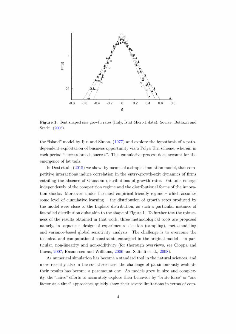
Figure 1: Tent shaped size growth rates (Italy, Istat Micro.1 data). Source: Bottazzi and

Secchi, (2006).

the “island”model by Ijiri and Simon, (1977) and explore the hypothesis of a path-

dependent exploitation of business opportunity via a Polya Urn scheme, wherein in

each period “success breeds success”. This cumulative process does account for the

emergence of fat tails.

In Dosi et al., (2015) we show, by means of a simple simulation model, that com-

petitive interactions induce correlation in the entry-growth-exit dynamics of firms

entailing the absence of Gaussian distributions of growth rates. Fat tails emerge

independently of the competition regime and the distributional forms of the innova-

tion shocks. Moreover, under the most empirical-friendly regime – which assumes

some level of cumulative learning – the distribution of growth rates produced by

the model were close to the Laplace distribution, as such a particular instance of

fat-tailed distribution quite akin to the shape of Figure 1. To further test the robust-

ness of the results obtained in that work, three methodological tools are proposed

namely, in sequence: design of experiments selection (sampling), meta-modeling

and variance-based global sensitivity analysis. The challenge is to overcome the

technical and computational constraints entangled in the original model – in par-

ticular, non-linearity and non-additivity (for thorough overviews, see Cioppa and

Lucas, 2007, Rasmussen and Williams, 2006 and Saltelli et al., 2008).

As numerical simulation has become a standard tool in the natural sciences, and

more recently also in the social sciences, the challenge of parsimoniously evaluate

their results has become a paramount one. As models grow in size and complex-

ity, the “naive” efforts to accurately explore their behavior by “brute force” or “one

factor at a time” approaches quickly show their severe limitations in terms of com-

4

putational times required and the poor expected accuracy (Helton et al., 2006,

Saltelli and Annoni, 2010). Hence, the search for mathematically “well behaved”

approximations of the inner relations of the original simulated model, frequently

denominated surrogate models or meta-models, has become increasingly common

(Kleijnen and Sargent, 2000, Roustant et al., 2012). The meta-model is a simplified

version of the original model that can be more parsimoniously explored – at reason-

able computational costs – to evaluate the effect of inputs/parameters on the latter

and (likely) also on the former. Usual techniques employed for meta-modeling are

linear polynomial regressions, neural networks, splines and Kriging.

Kriging (or Gaussian process regression), in particular, is suggested to be a sim-

ple but efficient method for investigating the behavior of simulation models (Van

Beers and Kleijnen, 2004). Kriging meta-models came originally from the geo-

sciences (Krige, 1951, Matheron, 1963). In essence, it is a Bayesian-based, spatial

interpolation method for the prediction of a system response on unknown points

based on the knowledge of such response on a set of previously known ones (the

observations) to fit a real-valued random field. Under some set of assumptions, the

Kriging meta-model can be shown to provide the best linear unbiased prediction

for such points (Roustant et al., 2012). The intuition behind it is that the original

model response for the unknown points can be predicted by a linear combination of

the responses at the closest known points, similarly to an ordinary multivariate lin-

ear regression, but taking the spatial information into consideration, in a Bayesian

framework. Recent advancements extended the technique, by removing the original

assumption that the samples are noise free, made Kriging particularly convenient for

the meta-modeling of stochastic computer experiments (Rasmussen and Williams,

2006).

Kriging, as any meta-modeling methodology, is based on the statistical estima-

tion of coefficients for specific functional forms (decribed in Section 4) based on data

observed from the original system or model. Kriging meta-models are frequently

estimated over a near-orthogonal Latin hypercube (NOLH) design of experiments1

(McKay et al., 2000, and nearer to our concerns here Salle and Yildizoglu, 2014).

The NOLH is a statistical technique for the generation of plausible sets of points

from multidimensional parameter distributions with good space-filling properties

(Cioppa and Lucas, 2007). It significantly improves the efficiency of the sampling

process in comparison to traditional Monte Carlo approaches, requiring far smaller

samples – and much less (computer) time – to the proper estimation of meta-model

coefficients (Helton et al., 2006, Iooss et al., 2010).

1In the present case it may be more appropriate to call the choice of the sampling points in the

parameters space as quasi-experiment, as the conditions imposed for selecting the observations for

the sample are specified by the NOLH.

5

Sensitivity analysis (SA) aims at “studying how uncertainty in the output of a

model (numerical or otherwise) can be apportioned to different sources of uncer-

tainty in the model input” (Saltelli et al., 2008). Due to the high computational

costs of performing traditional SA on the original model (e.g., ANOVA), authors

like Kleijnen and Sargent, (2000), Jeong et al., (2005) or Wang and Shan, (2007)

argue that the meta-model SA can be a reliable proxy for the original model be-

havior. Building on this assumption, one can propose the global SA analysis of the

Kriging meta-model – as we attempt here – to evaluate the response of the original

model over the entire parametric space, providing measurements of the direct and

the interaction effects of each parameter. Following Saltelli et al., (2000), for the

present analysis we selected a Sobol decomposition form of variance-based global

SA analysis. It decomposes the variance of a given output variable of the model

in terms of the contributions of each input (parameter) variance, both individually

and in interaction with every other input by means of Fourier transformations. This

method is particularly attractive because it evaluates sensitivity across the whole

parametric space – it is a global approach – and allows for the independent SA

analysis of multiple output models while being able to deal with non-linear and

non-additive models (Saltelli and Annoni, 2010).

The approach proposed here has proved insightful for the analysis of non-linear

simulation models, including economic ones: see Salle and Yildizoglu, (2014)2 on

two classic models and Bargigli et al., (2016) for an application to an agent-based

model of financial markets.

3 The original simulation model

The model of departure, extensively presented and discussed in Dosi et al., (2015),

represents the learning process by means of a multiplicative stochastic process upon

firms productivities ai ∈ R+, i = 1, . . . , N , in time t = 1, . . . , T :

ai(t) = ai(t− 1) {1 + max [0, θi(t)]} (1)

where θi ∈ R+ are realizations of a sequence of random variables {Θ}Ni=1, N is the

number of firms in the market and T is the number of simulation time steps. Such

dynamics is meant to capture the idiosyncratic accumulation of capabilities within

each firm (more in Dosi et al., 2000). The process is a multiplicative random walk

with drift: the multiplicative nature is well in tune with the evidence on productivity

dynamics under the further assumption that if a firm draws a negative θi, it will stick

2Here, we closely follow, whenever possible, the analytical framework employed by those authors

and refer the readers to their paper for additional details and references.

6

to its previous technique (negative shocks in normal times are quite unreasonable!),

meaning that the lower bound for the support of the shocks θi distribution is zero.

In Dosi et al., (2015) we experiment with different learning regimes. Different

specifications were tested for θi. In particular, we focus here on the regime called

Schumpeter Mark II, after the characterization of the “second Schumpeter” (Schum-

peter, 1947). In this specification, incumbents do not only learn, but do it in a

cumulative way so that a productivity shock in any firm is scaled by its extant

relative competitiveness:

θi(t) = min

[

πi(t)

(

ai(t− 1)

a(t− 1)

)γ

, µmax

]

,

a(t− 1) =∑

i

ai(t− 1)si(t− 1)(2)

where γ ∈ R+ is a parameter, 0 < si(t) ≤ 1 is the market share of firm i which

changes as a function of the ratio of the firm’s productivity (or “competitiveness”)

ai(t) to the weighted average of the industry a(t) and πi ∈ R is a random drawn

from a set of possible alternative distributions, being a rescaled Beta distribution

the default case.3 πi(t) distribution has average equal to µ ∈ R+. θi(t) is limited

by an upper bound µmax ∈ R+, based on the empirical evidence on the existence of

a finite limit to the innovation shocks amplitude.

Competitive interactions are captured by a “quasi-replicator” dynamics:

∆si(t, t− 1) = Asi(t− 1)

(

ai(t)

a(t)− 1

)

,

a(t) =∑

i

ai(t)si(t− 1)(3)

where A ∈ R+ is an elasticity parameter that captures the intensity of the selec-

tion exerted by the market, in terms of market share dynamics and, indirectly, of

mortality of low competitiveness firms. ai(t) is calculated over the lagged market

shares si(t− 1) for temporal consistency.

Finally, firms with market share si(t) lower than the parameter 0 < smin < 1

exit the market (“die”) and market shares are accordingly recomputed. We assume

that entry of new firms occurs (inverse) proportionally to the number of “surviving”

incumbents in the market:

E(t) = N − I(t− 1) (4)

where E(t) : N → N defines the number of entrants at time t, I(t − 1) ∈ N is the

number of incumbents in the previous period and N is defined as above. The empir-

ical evidence supports the idea that there is a rough proportionality between entry

3The rescaled Beta distribution was preferred because of its superior flexibility in terms of

parametrization and the bounded support. Other than Beta, Laplace and Gaussian, Log-normal

and Poisson distributions were also tested in Dosi et al., (2015). Different distributions did not

qualitatively affect the results.

7

and exit, thus, in the simplest version of the model, we assume a constant number

of firms with the number of dying firms offset by an equal number of entrants.

The productivity of entrant j follows a process similar to Eq. (1) but applied to

the average productivity of the industry at the moment of entry, whose stochastic

component θj is again a random drawn from the applicable distribution for πi as in

Eq. 2 (under γ = 0):

aj(t) = a(t)(1 + θj(t)) (5)

being a(t) calculated as in Eq. (3). Of course, here θj(t) can get negative values.

Indeed, the location of the mass of the distribution – over negative or positive

shocks – captures barriers to learning by the entrant or, conversely, the “advantage

of newness”. Entrant initial size is constant at sj(t0) = 1/N .

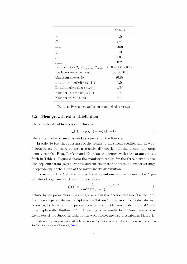
Table 1 summarizes all the model and the alternative distributions parameter

settings – our “default” configuration for the model – as well the remaining model

simulation setup.4 Because of the stochastic component in θi, the model outputs are

non-deterministic, so the aggregated results must evaluated in terms of the mean

and the variance of the output variables over a Monte Carlo (MC) experiment. It

is executed by a given number of model runs under different seeds for the random

number generator but with the same parameters configuration. Considering the

measured variance of the relevant output variables and a target significance level of

5%, a MC sample of 50 runs was determined as sufficient to fully qualify the model

results.

3.1 Timeline of events

• There are N initial firms at time t = 1 with equal productivity and market

share.

• At the beginning of each period firms learn according to Eq. (1).

• Firms acquire or lose market share, according to the replicator in Eq. (3).

• Firms exit the market according to the rule si(t) < smin.

• The number and competitiveness of entrants are determined as in Eqs. (4)

and (5).

• After entry market shares of incumbents are adjusted proportionally.

4The simulation model is coded in C++ and it is run inside the LSD simulation platform

(Valente, 2014) which is also employed for the NOLH sampling procedure, as explained below.

8

Value

A 1.0

N 150

smin 0.001

γ 1.0

µ 0.05

µmax 0.2

Beta shocks (βα, ββ , βmin, βmax) (1.0, 5.0, 0.0, 0.3)

Laplace shocks (α1, α2) (0.01, 0.015)

Gaussian shocks (σ) (0.8)

Initial productivity (ai(1)) 1.0

Initial market share (si(t0)) 1/N

Number of time steps (T ) 200

Number of MC runs 50

Table 1: Parameters and simulation default settings.

3.2 Firm growth rates distribution

The growth rate of firm sizes is defined as:

gi(t) = log si(t)− log si(t− 1) (6)

where the market share si is used as a proxy for the firm size.

In order to test the robustness of the results to the shocks specification, in what

follows we experiment with three alternative distributions for the innovation shocks,

namely rescaled Beta, Laplace and Gaussian, configured with the parameters set

forth in Table 1. Figure 2 shows the simulation results for the three distributions.

The departure from (log) normality and the emergence of fat tails is rather striking,

independently of the shape of the micro-shocks distribution.

To measure how “fat” the tails of the distributions are, we estimate the b pa-

rameter of a symmetric Subbotin distribution:

fS(x) =1

2ab1/bΓ(1/b+ 1)e−

1

b |x−µa |

b

(7)

defined by the parametersm, a and b, whereinm is a location measure (the median),

a is the scale parameter and b captures the“fatness”of the tails. Such a distribution,

according to the value of the parameter b, can yield a Gaussian distribution, if b = 2,

or a Laplace distribution, if b = 1, among other results for different values of b.

Estimates of the Subbotin distribution b parameter are also presented in Figure 2.5

5Subbotin parameters estimation is performed by the maximum-likelihood method using the

Subbotools package (Bottazzi, 2014).

9

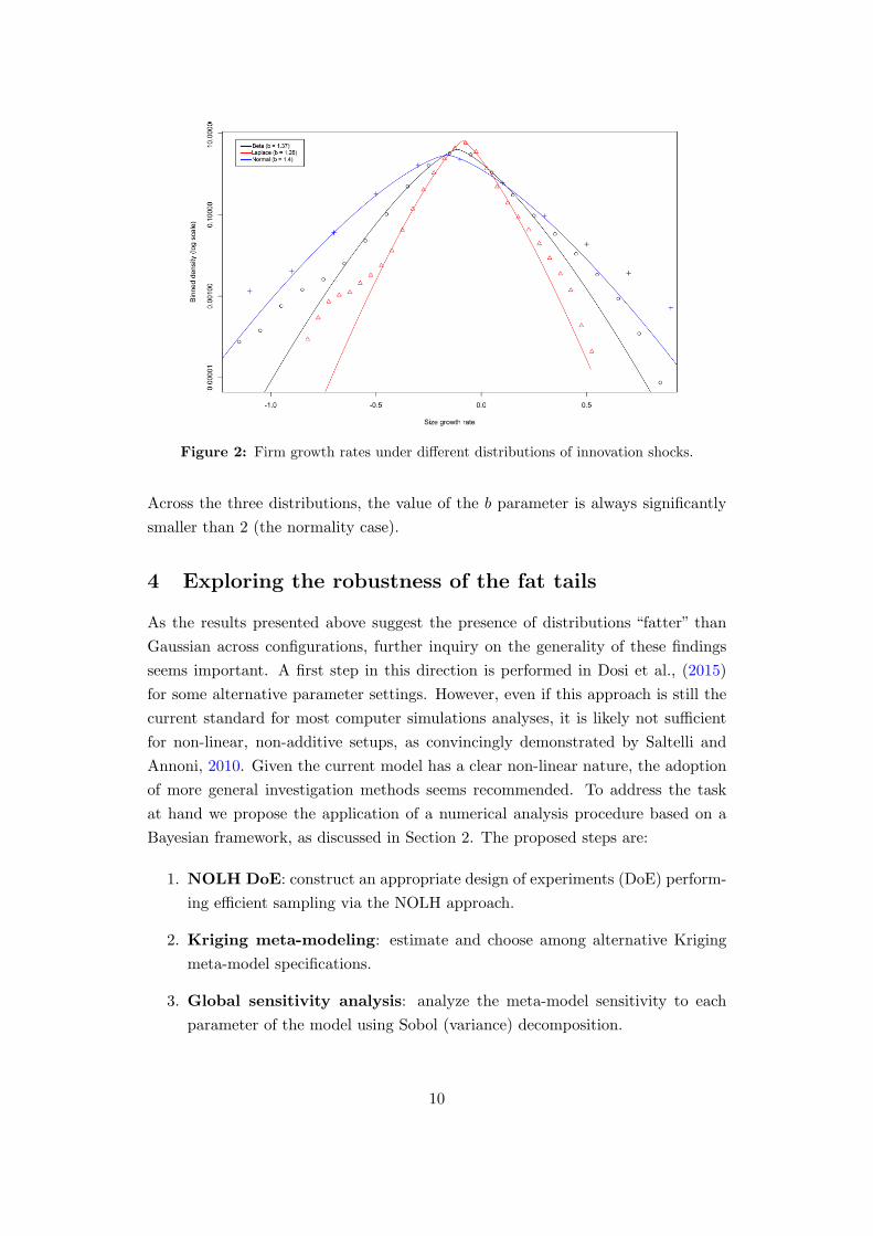
Figure 2: Firm growth rates under different distributions of innovation shocks.

Across the three distributions, the value of the b parameter is always significantly

smaller than 2 (the normality case).

4 Exploring the robustness of the fat tails

As the results presented above suggest the presence of distributions “fatter” than

Gaussian across configurations, further inquiry on the generality of these findings

seems important. A first step in this direction is performed in Dosi et al., (2015)

for some alternative parameter settings. However, even if this approach is still the

current standard for most computer simulations analyses, it is likely not sufficient

for non-linear, non-additive setups, as convincingly demonstrated by Saltelli and

Annoni, 2010. Given the current model has a clear non-linear nature, the adoption

of more general investigation methods seems recommended. To address the task

at hand we propose the application of a numerical analysis procedure based on a

Bayesian framework, as discussed in Section 2. The proposed steps are:

1. NOLH DoE: construct an appropriate design of experiments (DoE) perform-

ing efficient sampling via the NOLH approach.

2. Kriging meta-modeling: estimate and choose among alternative Kriging

meta-model specifications.

3. Global sensitivity analysis: analyze the meta-model sensitivity to each

parameter of the model using Sobol (variance) decomposition.

10

4. Response surface: graphically map the meta-model response surface (2D

and 3D) over the more relevant parameters and identify critical areas.

In a nutshell, the Kriging meta-model Y is intended to predict the response of

a given (scalar) output variable y of the original simulation model:6

Y (x) = λ(x) + δ(x) (8)

where x ∈ D is a vector representing any point in the parametric space domain D ⊂

Rk, being x1, . . . , xk ∈ R the k ≥ 1 original model parameters and λ(x) : Rk → R, a

function representing the global trend of the meta-model Y under the general form:

λ(x) =l

∑

i=1

βifi(x), l ≥ 1 (9)

being fi(x) : Rk → R fixed arbitrary functions and β1, . . . , βl the l coefficients to be

estimated from the sampled response of the original model over the image of y. The

trend function λ is assumed here, for simplicity, to be a polynomial of order l − 1,

more specifically of order zero (β1 is the trend intercept) or one (β2 is the trend

line inclination). This is usually enough to fit even complex response surfaces when

coupled with an appropriate design of experiment (DoE) sampling technique.7

In Eq. (8), δ(x) : Rk → R models the stochastic process representing the

local deviations from the global trend component λ. δ is assumed second-order

stationary with zero mean and covariance matrix τ2R (to be estimated), where τ2

is a scale parameter and R is a n×n matrix (n is the number of observations) whose

(i, j) element represents the correlation among δ(xi) and δ(xj), xi,xj ∈ D, i, j =

1, . . . , n. The Kriging meta-model assumes a close correspondence between this and

the correlation across y(xi) and y(xj) in the original model. Different specifications

can be used for the correlation function, according to the characteristics of the

y surface. For example, one of the simplest candidates is the power exponential

function:

corr(δ(xi), δ(xj)) = exp

−

k∑

g=1

ψg|xg,i − xg,j |

p

(10)

where xg,i denotes the value of parameter xg at the point xi, ψ1, . . . , ψk > 0 are

the k coefficients to be estimated and 0 < p ≤ 2 is the power parameter (p = 1 for

the ordinary exponential correlation function). They quantify the relative weight

of parameter xg, g = 1, . . . , k, on the overall correlation between δ(xi) and δ(xj)

6In this section we loosely follow the formalization proposed by Roustant et al., (2012) and Salle

and Yildizoglu, (2014).7Higher order polynomials were evaluated but systematically produced meta-models with worse

fitting to the original model, even when more samples are added to the DoE.

11

and, hopefully, among y(xi) and y(xj). Notice that a higher ψg represents a smaller

influence of parameter xg over δ.8

Therefore, the Kriging meta-model requires l+k+1 coefficients to be estimated

over the n observations selected by an appropriate design of experiments (DoE). As

discussed before, l = 1 or 2 is adopted. k is determined by the number of parameters

of the original model that are being evaluated in the sensitivity analysis, so it is

dependent on the specification of the innovation shocks (rescaled Beta, Laplace or

Gaussian). The original simulation model has four base parameters: A (replicator

sensitivity), N (number of firms), smin (the market share below which a firm exits

the market) and γ (learning cumulativity). The alternative shocks distributions have

two common parameters: µ and µmax (the average shock size and the upper support

limit). Additionally, rescaled Beta distribution requires βα, ββ (shape parameters),

βmin and βmax (support limits), Laplace needs α1 and α2 (shape parameters) and

Gaussian, σ (standard deviation), leading to a total of k = 10, 7 and 6 parameters

to test, respectively.

In practical terms, we constrained the experimental domain to ranges of the pa-

rameters that are empirically reasonable and respect minimal technical restrictions

of the original model,9 according to Table 2. The output variable tested (y) is the

selected “fat-taildness”measure of the distribution of firms’ growth rates (b) on the

original model. Therefore, y = b is estimated by the maximum-likelihood fit for the

b shape parameter of a Subbotin distribution (as defined above).

Three designs of experiments are created to evaluate each innovation shocks

specification. We use the rescaled Beta distributed shocks case to present the results

more extensively. The other cases, conversely, will be presented in a more concise

form. For the rescaled Beta (k = 10) and the Laplace (k = 7) configurations, DoE’s

with n = 33 samples are created. For the Gaussian (k = 6) case, while n = 17

is usually considered an adequate DoE size, we also select n = 33 because both

the Q2 and the RMSE goodness-of-fit measures (see below) perform much worse

under the smaller DoE when compared to the other two cases. The near-orthogonal

Latin hypercube (NOLH) DoE’s are constructed according to the recommendations

provided by Cioppa and Lucas, (2007). Yet, for the external validation procedures

(see below), 10 additional random samples are generated for each DoE. Because

of the stochastic nature of the original model, each point xi, i = 1, . . . , n in the

parametric space is computed over m = 50 simulation runs using different seeds for

8Definitions for other correlation function alternatives can be found in Roustant et al., 2012.9The technical feasibility criterion adopted was the minimally “normal” operation of the market,

measured by the survival of at least two firms during the majority of simulation time steps. Also,

some of the parameters’ test ranges limit, in practice, the possible ranges of variation for other

parameters (e.g., the distribution average µ must be lower than the upper support of distributions

µmax).

12

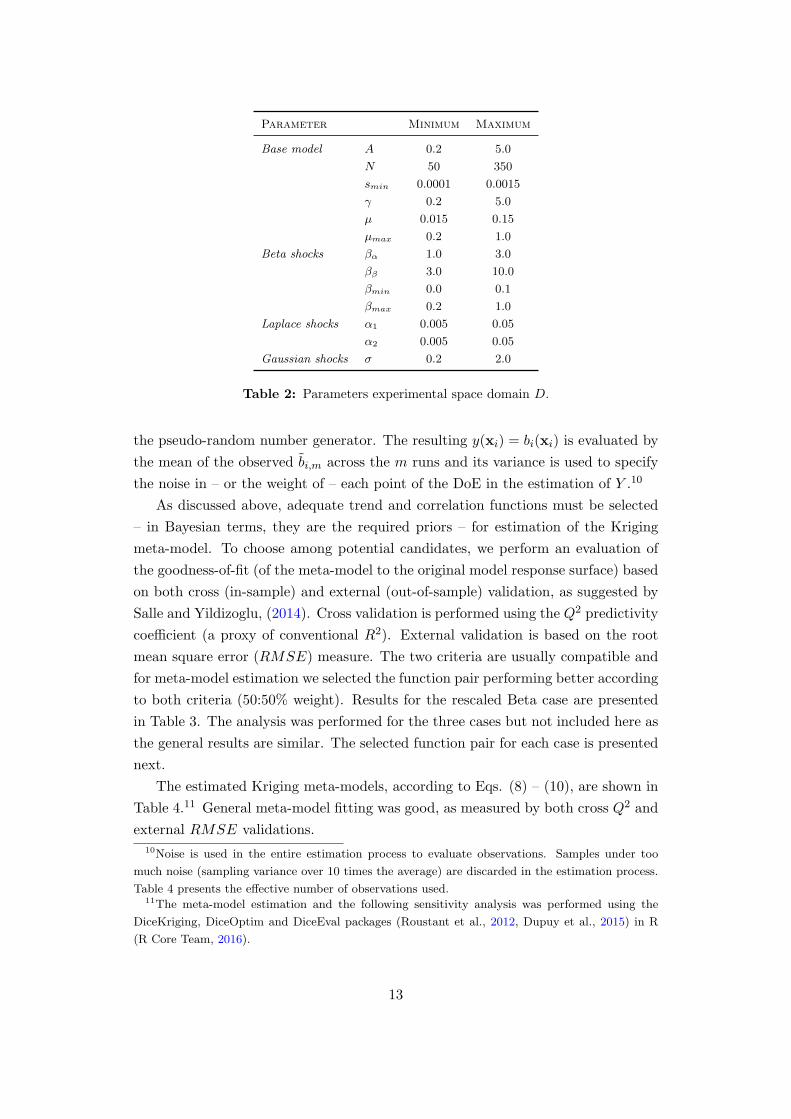
Parameter Minimum Maximum

Base model A 0.2 5.0

N 50 350

smin 0.0001 0.0015

γ 0.2 5.0

µ 0.015 0.15

µmax 0.2 1.0

Beta shocks βα 1.0 3.0

ββ 3.0 10.0

βmin 0.0 0.1

βmax 0.2 1.0

Laplace shocks α1 0.005 0.05

α2 0.005 0.05

Gaussian shocks σ 0.2 2.0

Table 2: Parameters experimental space domain D.

the pseudo-random number generator. The resulting y(xi) = bi(xi) is evaluated by

the mean of the observed bi,m across the m runs and its variance is used to specify

the noise in – or the weight of – each point of the DoE in the estimation of Y .10

As discussed above, adequate trend and correlation functions must be selected

– in Bayesian terms, they are the required priors – for estimation of the Kriging

meta-model. To choose among potential candidates, we perform an evaluation of

the goodness-of-fit (of the meta-model to the original model response surface) based

on both cross (in-sample) and external (out-of-sample) validation, as suggested by

Salle and Yildizoglu, (2014). Cross validation is performed using the Q2 predictivity

coefficient (a proxy of conventional R2). External validation is based on the root

mean square error (RMSE) measure. The two criteria are usually compatible and

for meta-model estimation we selected the function pair performing better according

to both criteria (50:50% weight). Results for the rescaled Beta case are presented

in Table 3. The analysis was performed for the three cases but not included here as

the general results are similar. The selected function pair for each case is presented

next.

The estimated Kriging meta-models, according to Eqs. (8) – (10), are shown in

Table 4.11 General meta-model fitting was good, as measured by both cross Q2 and

external RMSE validations.

10Noise is used in the entire estimation process to evaluate observations. Samples under too

much noise (sampling variance over 10 times the average) are discarded in the estimation process.

Table 4 presents the effective number of observations used.11The meta-model estimation and the following sensitivity analysis was performed using the

DiceKriging, DiceOptim and DiceEval packages (Roustant et al., 2012, Dupuy et al., 2015) in R

(R Core Team, 2016).

13

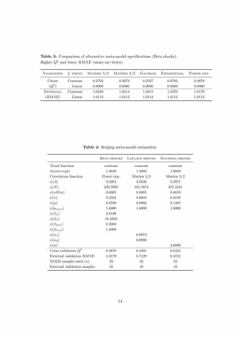
Table 3: Comparison of alternative meta-model specifications (Beta shocks).

Higher Q2 and lower RMSE values are better.

Validation fi trend Matern 5/2 Matern 3/2 Gaussian Exponential Power exp.

Cross Constant 0.2763 0.3073 0.2527 0.0793 0.2879

(Q2) Linear 0.0000 0.0000 0.0000 0.0000 0.0000

External Constant 1.0249 1.0514 1.0015 1.2370 1.0179

(RMSE) Linear 1.0112 1.0112 1.0112 1.0112 1.0112

Table 4: Kriging meta-model estimation.

Beta shocks Laplace shocks Gaussian shocks

Trend function constant constant constant

λ(intercept) 1.4649 1.4092 1.9603

Correlation function Power exp. Matern 5/2 Matern 5/2

ψ(A) 3.5984 3.5630 3.2971

ψ(N) 243.7065 101.5874 257.2181

ψ(sMin) 0.0005 0.0005 0.0010

ψ(γ) 9.2324 2.0045 8.0193

ψ(µ) 0.2700 0.0966 0.1485

ψ(µmax) 1.6000 1.6000 1.6000

ψ(βα) 3.8186

ψ(ββ) 10.4382

ψ(βmin) 0.2000

ψ(βmax) 1.4909

ψ(α1) 0.0872

ψ(α2) 0.0900

ψ(σ) 3.6000

Cross validation Q2 0.2879 0.4391 0.6454

External validation RMSE 1.0179 0.7129 0.4721

NOLH samples used (n) 33 32 32

External validation samples 10 10 10

14

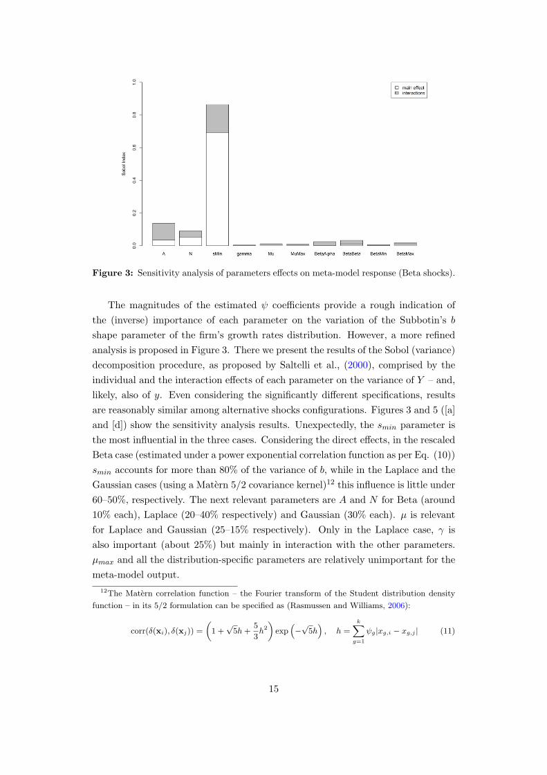
Figure 3: Sensitivity analysis of parameters effects on meta-model response (Beta shocks).

The magnitudes of the estimated ψ coefficients provide a rough indication of

the (inverse) importance of each parameter on the variation of the Subbotin’s b

shape parameter of the firm’s growth rates distribution. However, a more refined

analysis is proposed in Figure 3. There we present the results of the Sobol (variance)

decomposition procedure, as proposed by Saltelli et al., (2000), comprised by the

individual and the interaction effects of each parameter on the variance of Y – and,

likely, also of y. Even considering the significantly different specifications, results

are reasonably similar among alternative shocks configurations. Figures 3 and 5 ([a]

and [d]) show the sensitivity analysis results. Unexpectedly, the smin parameter is

the most influential in the three cases. Considering the direct effects, in the rescaled

Beta case (estimated under a power exponential correlation function as per Eq. (10))

smin accounts for more than 80% of the variance of b, while in the Laplace and the

Gaussian cases (using a Matern 5/2 covariance kernel)12 this influence is little under

60–50%, respectively. The next relevant parameters are A and N for Beta (around

10% each), Laplace (20–40% respectively) and Gaussian (30% each). µ is relevant

for Laplace and Gaussian (25–15% respectively). Only in the Laplace case, γ is

also important (about 25%) but mainly in interaction with the other parameters.

µmax and all the distribution-specific parameters are relatively unimportant for the

meta-model output.

12The Matern correlation function – the Fourier transform of the Student distribution density

function – in its 5/2 formulation can be specified as (Rasmussen and Williams, 2006):

corr(δ(xi), δ(xj)) =

(

1 +√5h+

5

3h2

)

exp(

−√5h

)

, h =

k∑

g=1

ψg|xg,i − xg,j | (11)

15

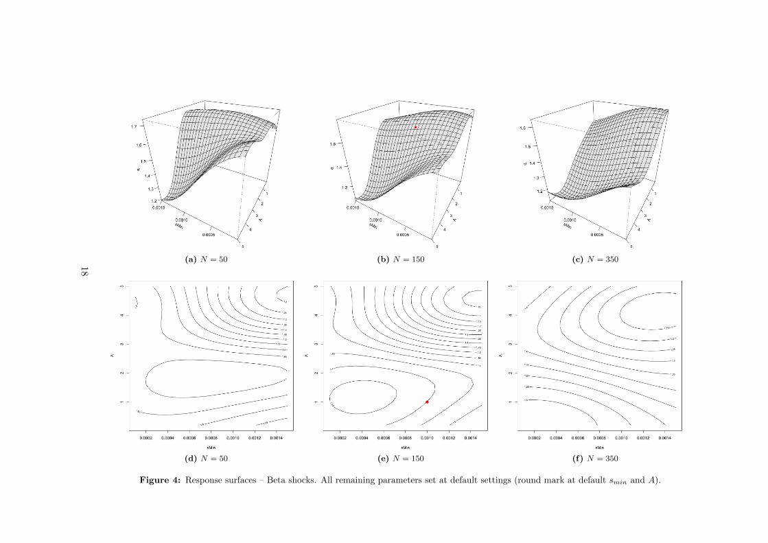
Considering the three dominant parameters detected by the Sobol decomposi-

tion, Figure 4 shows the response surfaces of the rescaled Beta shocks meta-model

for the full range of these parameters, as indicated in Table 2. The plots in the

columns of Figure 4 represent the same response surface, the top one in a 3D repre-

sentation and the one in the bottom using isolevel curves. In all plots, parameters

smin ∈ [0.0001, 0.0015] and A ∈ [0.2, 5] are explored over their entire variation

ranges. The first and the last columns (Figure 4, plots [a], [c], [d] and [f]) show the

response for the limit values of parameter N ∈ [50, 350], while the center column

(plots [b] and [e]) depicts the default model setup (except for smin and A). The

round mark in the two plots represents the meta-model response at the full default

settings, as per Table 1. The prediction of the meta-model for this particular point

in the parameters space – which is not included in the DoE sample – is b = 1.58

while the “true” value from the original model is b = 1.37, an error of +15% wholly

inside the expected 95% confidence interval for that point (ǫ = ±0.75).13 In partic-

ular, the default settings point is located at a level close to the global maximum of

the response surface, around b = 1.75 (the minimum is at b = 1).

Coupled with the sensitivity analysis results, which show that smin, A and N

are the only parameters significantly affecting the predicted b, Figure 4 seems to

corroborate the hypothesis that the model results are systematically fat-tailed, as

can be inferred from the condition b < 2. However, considering the average 95%

confidence interval ǫ = ±0.68 range for the meta-model response surface, it seems

that still exists a region where we cannot discard the absence of fat-tails (b ≥ 2)

at the usual significance levels. Therefore, further analysis is required, this time

focused in this particular area, representing a small portion of the parametric space

where the meta-model resolution is not sufficient to completely specify the response

of the original model. Considering the critical region only (approximated to smin ∈

[0.0001, 0.001] and A ∈ [0.2, 3]), a “brute force” Monte Carlo sampling approach is

performed in the original model. Not surprisingly, out of 20 random observations,

considered sufficient given the predicted smoothness of the investigated area at a 5%

significance level, the sampled interval true response was in the range [1.25, 1.63],

confirming that the meta-model predicted b, in this particular region, is likely to

overestimate the true value of the shape parameter b. In conclusion, it seems very

probable that the true response surface of the original model is significantly under

the b = 2 limit over the entire explored parametric space for rescaled Beta innovation

shocks.

Similar analysis is conducted for the Laplace and Gaussian innovation shocks

13Kriging predictions becomes more precise as the interpolated point gets closer to one of the

DoE points, where the error of the model is always zero by construction – and vice versa – so ǫ is

not constant.

16

meta-models. The results are synthesized in Figure 5. The Laplace case is in the

upper row (plots [a], [b] and [c]) which presents the Sobol decomposition sensitivity

analysis, already discussed, and the surface response for the top two critical param-

eters (smin ∈ [0.0001, 0.0015] and N ∈ [50, 350]). Again, the meta-model predicted

response with default settings is at a level b = 1.51, close to the global maximum at

b = 1.77 and above the minimum at b = 0.91. The true value at the default point is

b = 1.28 and the prediction error is +18%, well under the 95% confidence interval

ǫ = ±0.69 in that point. As in the previous case, and despite the entire meta-model

surface is substantially below the critical level b = 2, under the usual significance

levels (ǫ = ±0.77) there is a region of the surface where we cannot discard b ≥ 2.

However, once again the Monte Carlo exploration of this critical region on the orig-

inal model, also seems to confirm the hypothesis of b < 2 for the whole parametric

space of the original model under Laplace innovation shocks.

Qualitatively close results come from the Gaussian meta-model. The dynamics

of the meta-model here is driven by smin ∈ [0.0001, 0.0015] and N ∈ [50, 350]. The

produced response surface is slightly more rugged, as depicted in Figure 5 ([d], [e]

and [f]). The meta-model prediction for the default settings point is b = 1.36, well

in between the surface’s global minimum at b = 0.98 and the maximum at b = 1.71.

The prediction error, in this case, is −3% given the true b = 1.40, easily inside the

95% confidence interval ǫ = ±0.74. Again, considering the average 95% confidence

interval ǫ = ±0.47 over the entire surface, there is a small region of the response

surface (the “hilltop” around N < 70 and smin > 0.0010) where it’s not possible

to reject the absence of fat tails. However, specific MC exploration in this area on

the original model once more produced no points sitting close to the b = 2 limit,

confirming the meta-model predictions of b < 2 for the entire region.

17

(a) N = 50 (b) N = 150 (c) N = 350

(d) N = 50 (e) N = 150 (f) N = 350

Figure 4: Response surfaces – Beta shocks. All remaining parameters set at default settings (round mark at default smin and A).

18

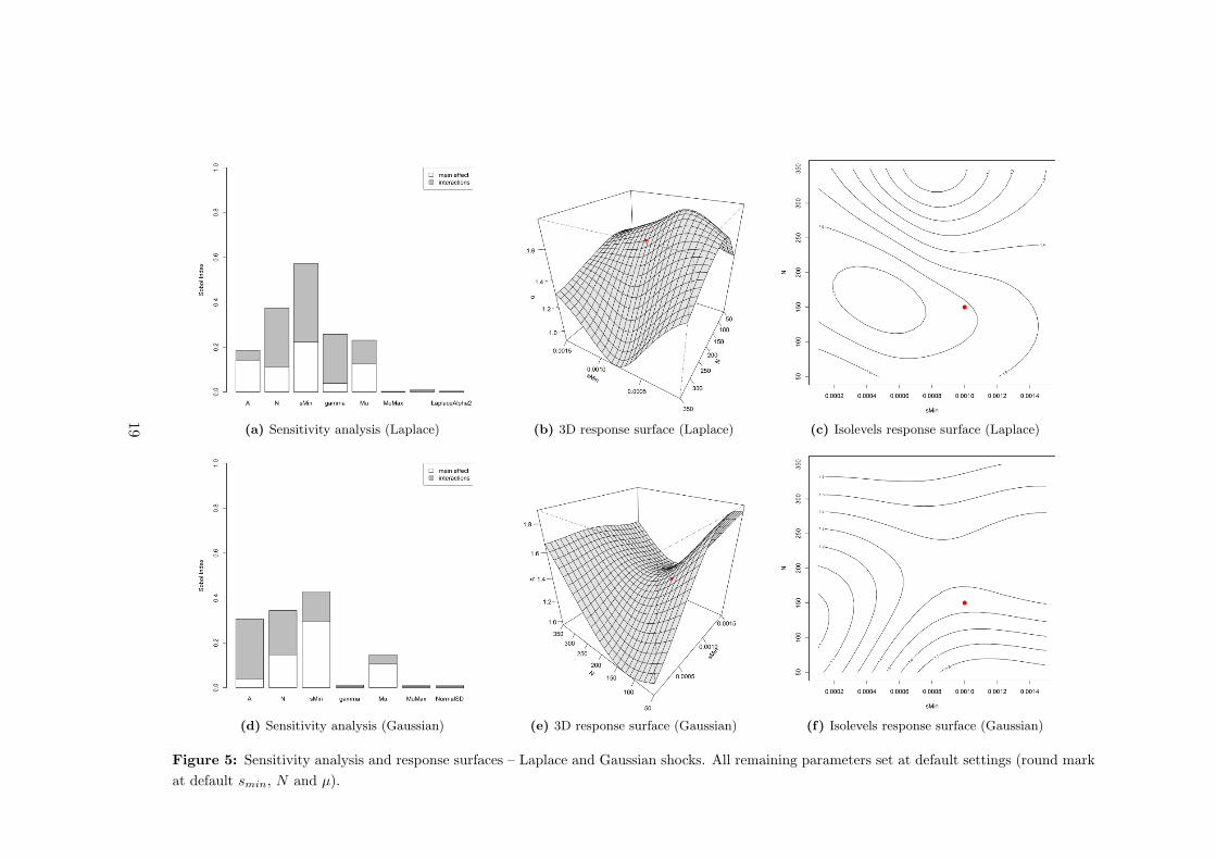
(a) Sensitivity analysis (Laplace) (b) 3D response surface (Laplace) (c) Isolevels response surface (Laplace)

(d) Sensitivity analysis (Gaussian) (e) 3D response surface (Gaussian) (f) Isolevels response surface (Gaussian)

Figure 5: Sensitivity analysis and response surfaces – Laplace and Gaussian shocks. All remaining parameters set at default settings (round mark

at default smin, N and µ).

19

5 Discussion

Our results show that the model is able to reproduce, over most of the parameters

space, fat-tailed growth rates distributions – and even strict Laplace ones. The Krig-

ing meta-models confirm and strengthen the results obtained in Dosi et al., (2015),

providing evidence that the coupling of the two evolutionary processes of learning

and selection is a strong candidate to explain the observed fat-tailed distributions

of firm growth rates.

From the analysis made possible by the meta-models, the modeller can acquire

a set of relevant new information on the original model behaviour. However, care

should be taken to account for the expected prediction errors on the response sur-

faces: isolevels and 3D surfaces should be understood with the associated confidence

intervals (at the desired significance level), that are not regular (constant) in Kriging

meta-models. In any case, the order of magnitude of the out-of-sample RMSE in Ta-

ble 4 remains a good indication of the limits to be expected on the overall confidence

intervals. Moreover, even when the confidence intervals may be not sufficiently nar-

row to objectively accept or reject a given proposition, the topological information

provided by the meta-model response surface has proved to be a powerful tool on

guiding (and making possible) the exploration of the original model by means of

other (more data-demanding) tools, like conventional Monte Carlo sampling.

According to the global effect of parameters on meta-models responses, provided

by variance decomposition, the elicited parameters in the three analysed cases in or-

der of significance are: [i] smin (exit market share), [ii] A (replicator sensitivity), [iii]

N (number of firms), and [iv] γ (degree of cumulativity). When they are relevant,

according to the shocks distribution case, both direct and interaction effects influ-

ence the response surfaces. From the analysis of the latter, some regular patterns

of the parameters’ effects on the value of meta-models’ b can be identified.

First, the smin parameter exerts a mostly monotonic influence on the change of

b: the higher the death-threshold the fatter the tails of growth rate distribution are.

This result, admittedly unexpected in its strength, is likely to capture the impact

of that extreme form of selection which is “death”, upon the whole distribution of

growth rates.

Second, the higher the value of the A parameter, in general the lower the value

of b. Similarly to smin, this parameter controls for the degree of selection operating

among incumbent firms. In fact, higher selection in the market induces a greater

reallocation of shares among surviving incumbents. In the region where competition

is fierce both in the entry-exit and in the reallocation processes, characterised by

high values for smin and A respectively, very low levels of the b parameter are

recorded and almost “pure” Laplacian tails emerge.

20

Third, the mechanism of cumulation in learning activities, modulated by γ,

exerts a positive influence on the tail-fatness in our meta-model specifications, as

already detected in Dosi et al., (2015). The process of cumulation of knowledge

influences directly firms productivity growth, and indirectly their performance in

the market.

The results from the Kriging meta-models confirm and strengthen the previous

findings discussed in Dosi et al., (2015) but a word of caution is necessary when

interpreting the meta-model and in particular the effect of the coefficients ψg on

corr(y(xi), y(xj)). In fact, a simplification of the deterministic component λ(x) puts

the burden of explanation on the stochastic part δ(x). Admittedly, focusing on the

modeling of λ would yield an increasing dimensionality of the meta-model, compris-

ing all the k = 10, 7 or 6 parameters themselves, their interaction and higher order

terms. Intuitively, the Kriging rationale in privileging the modeling of cov(δ(x)),

instead, is that it allows for the capture the behavior of Y (x) using much fewer ob-

servations while still keeping global covariance-based sensitivity analysis possible.

Indeed, a constant deterministic function can be not only the result of the sum of

constant x1, . . . , xk ∈ R parameters but also, being λ(x) : Rk → R the function

representing the global trend of the meta-model Y , it may well proximately capture

different dynamics for some parameters xg: in such a case a constant deterministic

component could “artificially” flatten the meta-model. Of course the associated loss

of information about the model sharply falls as the number of parameters or of the

DoE samples increase.

Furthermore, even if the correlation function coefficients are estimated using

data coming from the original model, the ensuing covariances are fully precise only at

the exact DoE (sampling) points, as for all others we are using an interpolation of the

closest DoE points to predict the correlation values. That is why, in fact, the meta-

model is just a surrogate model, an approximation which cannot – and so should

not be used to – substitute the original model: the estimated coefficients in Table 4

represent the overall expected effects of each parameter xg on the variance of meta-

model’s response and thus in the final predicted values Y (x), all subject to the usual

restrictions of any non-parametric Bayesian approximation, in particular the chosen

priors (the trend and the correlation functional forms). The coefficients ψ being

estimated govern “associations” among the original parameters (the covariation in

the components of the random effect δ(x)), but they do not represent direct effects

of the original parameters xk on Y (x).

Notwithstanding these caveats, the meta-model approximate response surface is

still a powerful guide for the general exploration of the original model, as a kind

of “reduced map”, providing illuminating guidance on the sign of the effects of the

parameters on the output variable(s), on their relative importance, and on the ones

21

critical for particular “suspicious” points. Relatedly, the exercise hints to the region

of the parameters space to intensively search, on the ground of the original model,

performing traditional local sensitivity analysis, at this stage more feasible given

the lower number of dimensions and factor ranges. That is, despite some possible

– or even likely – “false-positives” from the meta-models, any search in the original

model becomes at least better informed with them.

6 Conclusions

Empirically, one ubiquitously observes fat-tailed distributions of firm growth rates.

In Dosi et al., (2015) we built a simple multi-firm agent-based model able to repro-

duce this stylised fact. In this contribution we use Kriging meta-modeling method-

ology associated with a computationally efficient Near-Orthogonal Latin Hypercube

design of experiment which allows for the fully simultaneous analysis of all of the

models parameters under their entire useful ranges of variation. The exercise con-

firms the high level of generality of the results previously obtained by means of

a statistically robust global sensitivity analysis. The mechanisms of market selec-

tion, both in the entry-exit and in the market share reallocation processes, together

with cumulative learning, turn out to be quite robust candidates to explain the

tent-shaped distribution of firms’ growth rates.

Acknowledgements

We thank Francesca Chiaromonte for helpful comments and discussions. We grate-

fully acknowledge the support by the European Union’s Horizon 2020 research and

innovation programme under grant agreement No. 649186 - ISIGrowth and by

Fundacao de Amparo a Pesquisa do Estado de Sao Paulo (FAPESP), process No.

2015/09760-3.

References

Bargigli, L., L. Riccetti, A. Russo, and M. Gallegati (2016). Network Calibration

and Metamodeling of a Financial Accelerator Agent Based Model. Available at

SSRN.

Bottazzi, G., E. Cefis, and G. Dosi (2002). “Corporate growth and industrial struc-

tures: some evidence from the Italian manufacturing industry”. Industrial and

Corporate Change 11.4, 705–723.

Bottazzi, G. and A. Secchi (2003). “A stochastic model of firm growth”. Physica A:

Statistical Mechanics and its Applications 324.1, 213–219.

22

Bottazzi, G. and A. Secchi (2006).“Explaining the distribution of firm growth rates”.

RAND Journal of Economic 37.2, 235–256.

Bottazzi, Giulio (2014). SUBBOTOOLS. Scuola Superiore Sant’Anna. Pisa, Italy.

url: http://cafim.sssup.it/~giulio/software/subbotools/.

Cioppa, T. and T. Lucas (2007). “Efficient nearly orthogonal and space-filling Latin

hypercubes”. Technometrics 49.1, 45–55.

Dosi, G. (2007). “Statistical Regularities in the Evolution of industries. A guide

trough some evidence and challenges for the theory”. In: Perspectives on inno-

vation. Malerba, F. and Brusoni, S. Editors (2007).

Dosi, G., O. Marsili, L. Orsenigo, and R. Salvatore (1995). “Learning, market selec-

tion and the evolution of industrial structures”. Small Business Economics 7.6,

411–436.

Dosi, G., R. Nelson, and S. Winter (2000). The nature and dynamics of organiza-

tional capabilities. Oxford University Press.

Dosi, G., M.C. Pereira, and M.E. Virgillito (2015). The footprint of evolutionary

processes of learning and selection upon the statistical properties of industrial

dynamics. LEM Papers Series 2015/04. Laboratory of Economics and Manage-

ment (LEM), Sant’Anna School of Advanced Studies, Pisa, Italy.

Dupuy, D., C. Helbert, and J. Franco (2015). “DiceDesign and DiceEval: Two R

Packages for Design and Analysis of Computer Experiments”. Journal of Statis-

tical Software 65.11, 1–38. url: http://www.jstatsoft.org/v65/i11/.

Hanusch, H. and A. Pyka (2007). Elgar Companion to Neo-Schumpeterian Eco-

nomics. Edward Elgar.

Helton, J., J. Johnson, C. Sallaberry, and C. Storlie (2006). “Survey of sampling-

based methods for uncertainty and sensitivity analysis”. Reliability Engineering

& System Safety 91.10, 1175–1209.

Ijiri, Y. and H. Simon (1977). Skew Distributions and the Sizes of Business Firms.

Amsterdam: North-Holland.

Iooss, B., L. Boussouf, V. Feuillard, and A. Marrel (2010). “Numerical studies of the

metamodel fitting and validation processes”. arXiv preprint arXiv:1001.1049.

Jeong, S., M. Murayama, and K. Yamamoto (2005). “Efficient optimization design

method using kriging model”. Journal of Aircraft 42.2, 413–420.

Kleijnen, J. and R. Sargent (2000). “A methodology for fitting and validating meta-

models in simulation”. European Journal of Operational Research 120.1, 14–29.

Krige, D. (1951). “A statistical approach to some basic mine valuation problems on

the Witwatersrand”. Journal of the Chemical, Metallurgical and Mining Society

of South Africa 52.6, 119–139.

Malerba, F. and S. Brusoni (2007). Perspectives on innovation. Cambridge Univer-

sity Press.

23

Matheron, G. (1963). “Principles of geostatistics”. Economic geology 58.8, 1246–

1266.

McKay, M., R. Beckman, and W. Conover (2000). “A comparison of three methods

for selecting values of input variables in the analysis of output from a computer

code”. Technometrics 42.1, 55–61.

Metcalfe, J. S. (1998). Evolutionary Economics and Creative Destruction. Rout-

ledge.

Nelson, R. R. and S. G. Winter (1982). An Evolutionary Theory of Economic

Change. Cambridge, MA: Belknap Press of Harvard University Press.

R Core Team (2016). R: A Language and Environment for Statistical Computing. R

Foundation for Statistical Computing. Vienna, Austria. url: https://www.R-

project.org/.

Rasmussen, C. and C. Williams (2006). Gaussian processes for machine learning.

Cambridge, MA: MIT Press.

Roustant, O., D. Ginsbourger, and Y. Deville (2012).“DiceKriging, DiceOptim: Two

R packages for the analysis of computer experiments by kriging-based metamod-

eling and optimization”. Journal of Statistical Software 51.1, 1–55.

Salle, I. and M. Yildizoglu (2014). “Efficient Sampling and Meta-Modeling for Com-

putational Economic Models”. Computational Economics 44.4, 507–536.

Saltelli, A. and P. Annoni (2010). “How to avoid a perfunctory sensitivity analysis”.

Environmental Modelling & Software 25.12, 1508–1517.

Saltelli, A., M. Ratto, T. Andres, F. Campolongo, J. Cariboni, D. Gatelli, M.

Saisana, and S. Tarantola (2008). Global sensitivity analysis: the primer. New

York: John Wiley & Sons.

Saltelli, A., S. Tarantola, and F. Campolongo (2000). “Sensitivity analysis as an

ingredient of modeling”. Statistical Science 15.4, 377–395.

Schumpeter, J. (1947). Capitalism, Socialism, and Democracy. New York and Lon-

don: Harper & Brothers Publishers.

Silverberg, G., G. Dosi, and L. Orsenigo (1988).“Innovation, Diversity and Diffusion:

A Self-organisation Model”. Economic Journal 98.393, 1032–54.

Valente, Marco (2014). LSD: Laboratory for Simulation Development. University of

L’Aquila. L’Aquila, Italy. url: https://www.labsimdev.org/.

Van Beers, W. and J. Kleijnen (2004). “Kriging interpolation in simulation: a sur-

vey”. In: Simulation Conference, 2004. Proceedings of the 2004 Winter. Vol. 1.

IEEE.

Wang, G. and S. Shan (2007). “Review of metamodeling techniques in support of

engineering design optimization”. Journal of Mechanical design 129.4, 370–380.

24