real numbers. constants, variables, and mathematical …ama5348/umn2002f/math1051/lec1_4.pdf · y...

Lecture 1.

Real numbers. Constants, variables, andmathematical modeling.

In this lecture we briefly sketch the structure of Real numbers and recall properties ofaddition and subtraction. Then we will discuss the notions of variables and constants and basicideas of mathematical modeling.

1.1. Real Numbers

We will try to sketch the structure of numbers by ranging them by the increase of com-plexity. Most people agree that the simplest are the counting numbers.

1, 2, 3, 4, 5

The next step is the whole numbers (a “zero” element was added)

0, 1, 2, 3, 4, 5

to make whole numbers even more useful the addition and multiplication were invented.The addition and the multiplication were invented in such a way to satisfy commutativeproperties

a+ b = b+ a

a · b = b · a,

and the associative properties

a+ (b+ c) = (a+ b) + c

a · (b · c) = (a · b) · c,

and the distributive properties

a · (b+ c) = a · b+ a · c.

Lecture 1. Real numbers. Mathematical modeling. 2

Remark 1.1. Note that 0 plays a special role for the summation and 1 plays a specialrole for the multiplication as it demonstrated by the Identity properties:

0 + a = a+ 0 = a, a · 1 = 1 · a = a.

Thinking about loand and debts the human kind invented Additive Inverse

−a is a number such that (−a) + a = 0.

Example 1.1. Suppose you owe someone 6 pots of honey and some one else givesyou another 6 pots of honey. How much honey do you have now? The right answer is(−6) + 6 = 0.

The subtraction is an immediate consequence of addition and additive inverse: bydefinition,

a− b = a+ (−b).

Smoothly, we arrive to the next stage:

Whole numbers + their additive inverses = Integer numbers

. . .− 3,−2,−1, 0, 1, 2, 3, . . .

Thinking about sharing the humanity invented the multiplicative inverse(1

b

)is the number such that

(1

b

)· b = 1.

The division then is an immediate consequence of multiplication and the multiplicativeinverse:

a

b= a ·

(1

b

).

The right side reads a times multiplicative inverse of b.

Remark 1.2. Not all integer numbers have multiple inverse. In particular, 0 doesn’t.Indeed, 1/0 is undefined since there is no such number which is being multiplied by 0gives you 1: (?) · 0 = 1.

When the Integer numbers are combined with their multiplicative inverses we getRational numbers, or numbers of the form

m

n, where m and n are integer numbers.

It can be verified that all addition and multiplication properties make sense for the rationalnumbers.


Question 1.1. What is the additive and multiplicative inverses to

m

n?

The Irrational numbers is the next stage after the Rational numbers. The examplesof irrational numbers are

π,√

2, e.

Unfortunately, in the frames of this course we can not discuss how the irrational numbersare defined. For us it will be enough to think about the irrational numbers as

Decimal number with infinite, non repeating decimals

In fact, every irrational number can be approximated by a rational so close so there willbe no practical difference for us what number to use. For example, the numbers you areusing in calculator all are rational

Summarizing, the Real numbers are

IRRATIONAL + RATIONAL + (INTEGER) + (WHOLE) + (COUNTING)

we put last three in the parenthesis since they already present in rationales.

1.2. Some review

Let us go back and review some rules for acting with rational numbers. The formulas forthe multiplication and division of rational numbers are

a

b· cd

=ac

bd,

abcd

=a

b·(

1cd

)=a

b· dc

=ad

bc.

The simplest formula for the addition and subtraction:

a

c± b

c=a± bc

.

Note that the denominators in this formula are the same.

Question 1.2. What if the denominators are not the same?

Then we can make it the same:

a

b± c

d=a

b· dd± c

d· bb

=ad

bd± cb

db=ad± cbbd

.

Example 1.2.2

3· 5

7=

2 · 53 · 7

=10

21


3

8+

5

7=

3

8· 7

7+

5

7· 8

8=

21 + 40

56=

61

50=

61

7 + 8

45310

=4

5·(

1310

)=

4

5· 10

5=

40

15=

8

3.

4

2− 2

3=

4

3

In the last example make sure that you did not “cancel twos out”.

To solve the next problem we will need to recall the definition of the natural exponent:an = a · a · . . . · a︸︷︷︸

n

.

Example 1.3. (1.5 ex.70 ).

−8− 23 − [1− 42 · (0)] = −8− 8− 1 = −17.

1.3. Real number line

The real numbers can be naturally identified with a points on the line. Indeed, pick apoint O and call it the “Origin”, pick another point U to the right of the origin andcall it “Unit” then we associate number 0 with the origin and 1 with U . The point tothe right from U that is twice as far from 0 as U is associated with the number 2. Thepoint to the right of U that is midway between 0 and U is assigned 1/2, and so on. Thecorresponding points to the left of the origin are assigned the numbers −1/2,−1,−2, andso on depending on how far they are from 0.

Definition 1.1. The real number associated with a point P is called the coordinateof P , and the line whose points have been assigned coordinates is called the real numberline.

1.4. Inequalities

An important property of real number line follows from the fact that given two points(numbers) a and b either

a is to the left of b,

a equals (coincides with) b,

a is to the right of b.


Using this property we can define an “order” on the real numbers. We will say that

a is less then b ⇔ a < b ⇔ if a is to the left of b,

a equals b ⇔ a = b ⇔ if a coincides with b,

a is greater than b ⇔ a > b ⇔ if a is to the right of b.

As an exercise try to prove

a < b ⇔ a− b < 0,

a = b ⇔ a− b = 0,

a > b ⇔ a− b > 0.

By the way, there are two more useful relations

a ≤ b ⇔ a is less then or equal to b

a ≥ b ⇔ a is greater then or equal to b

But these are just combinations of the above ones.

Example 1.4. Replace the question mark by <, >, or =, which ever is correct.(1.6 ex.7 )

1

2? 0.5.

Answer: the correct relation is1

2= 0.5.

(1.6 ex.8 )1

3? 0.33

To solve this problem we need to bring both number to the same denominator and thencompare them:

1

3?

33

100⇔ 1

3· 100

100?

33

100· 3

3⇔ 100

300>

99

300.

Definition 1.2. A statement in which two expressions are related by an inequalitysymbol is called an inequality.

Example 1.5. (1.6 ex.18 ) Write the statement as an inequality: x is greater then orequal to 2. Answer:

x ≥ 2.


1.5. Absolute value

Definition 1.3. The absolute value of a number a denoted by |a| is determined bythe following formula

|a| =

{a if a ≥ 0,

−a if a < 0.

Absolute value of a number a is the distance from the point with coordinate a to theorigin.

1.6. Distance between two points on a real number line

Distance between two points P and Q with the coordinates by a and b respectively isgiven by

d(P,Q) = |b− a|As an exercise try to check that d(P,Q) = d(Q,P ).

Example 1.6.(1.6 ex.32 ) Given a picture evaluate distance between points D and A.

d(D,A) = |1− (−3)| = |4| = 4

(1.6 ex.50 ) Evaluate 3|x|+ 2|y| for x = 2 and y = −3:

3|2|+ 3| − 3| = 12.

1.7. Constants, variables

Let us picture a guy measuring the weight of wooden cubes of different sizes. He takescube and puts it onto a weighing devise. Cube of size 1 gives weight 1 cube of size 2 givesweight 8, cube of size 3 gives the weight 27. Eventually he gets cube of size 10. He tries toput cube on the weighing device and realizes that whether himself or the weighing devicewill be broken by that heavy cube.

What the guy does next? He makes some mathematical modeling and he ends upwith a nice formula

W = l3,

where l is called a variable and it stays for the length of the side of a cube, W is a variableas well and it stands for the weight.


Variable is a letter standing for varying values in a mathematical expression. Variablealways has a “Domain”. Domain of the variable is the set of numbers which can besubstituted for the letter.

If our guy thinks a little more he will probably end up with more advanced formula

W = ρl3,

which now will work for cubes made from a different material. Here letter ρ keeps theinformation about the material. If all cubes made from the same material then ρ does notchange from cube to cube. In this case we will say that ρ is a constant in our formula.

Constant is a letter presenting some particular number.

1.8. Mathematical Modeling

Picture * illustrates the process of mathematical modeling. Suppose we observe somenatural phenomena (picture to the left) and we want to predict it. Then we will need toconstruct a model (picture to the right). For the construction we use elements which weunderstand absolutely clear (otherwise we will not understand how the model works andwe will need to build a model for the model). When the model is ready we try some inputto check if the output of our model looks similar to the output of the natural phenomena.The model, of course, is never the same as the real phenomena and very often we haveto improve and improve it until there will be a practically good correspondence with thereal process.

Example 1.7. (1.7 ex.2 ) Determine the domain of x

−8

x+ 5

Answer: Domain is x 6= −5.

(1.7 ex.36 ) The height of an object vertically propelled upward with an initial velocityv after t seconds assuming no air resistance, is given by formula

h = vt− 1

2(32)t2.

Calculate h after 2 seconds under the following conditions

initial velocity: v = 50,

h = 50× 2− 1

2(32)(2)2 = 100− 64 = 36.

Lecture 2.

Polynomials. Operations on polynomials

On this lecture we will recall the definition of polynomial, and operations on them: addition,subtraction, and multiplication. We will discuss horizontal and vertical rules for the additionand multiplication.

2.1. Polynomials

Definition 2.1. A polynomial in one variable is an algebraic expression of the form

P (x) = anxn + an−1x

n−1 + . . .+ a1x+ a0. (2.1)

A monomial is a polynomial with only one term

M(x) = axm.

Question 2.1. What are constants and what are variables here?

The constants ai are called coefficients of the polynomial P (∗);

the number n is the degree of the polynomial P (x);

coefficient an is called a leading coefficient;

term anxn is called a leading term.

Example 2.1. Consider polynomial P (x) = x5 − 1, determine its degree and listcoefficients. The degree of polynomial P (x) is 5, so n = 5, and coefficients are a5 = 1,a4 = 0, a3 = 0, a2 = 0, a1 = 0, a0 = −1.

Consider number +1. If this is a particular case of polynomial? The answer is Yes.This is a polynomial of the degree zero.

Definition 2.2. Formula (2.1) gives the “standard form” for polynomial P (x).

Of course, there are many other ways how to express the same polynomial P (x).

Lecture 2. Polynomials. Operations on polynomials 9

Example 2.2. (2.1 ex. 47 ) Write the polynomial in standard form, list the coeffi-cients, give the degree

P (x) = 1− x+ x2 − x3

Answer: degree is 3; coefficients are a3 = −1, a2 = 1, a1 = −1, a0 = 1,

P (x) = −x3 + x2 − x+ 1.

2.2. Operations on polynomials

A polynomial can be myltiplied with a number:

b · P (x) = b · (anxn + . . .+ a0) = (ban)xn + (ban−1)xn + . . .+ (ba0).

Two polynomials can be added to or subtracted from each other. The rule is simple:polynomials are added and subtracted by combining like terms after applying commutativeand associative properties of the addition.

P (x) = anxn + an−1x

n−1 + . . .+ a1x+ a0,

Q(x) = bnxn + bn−1x

n−1 + . . .+ b1x+ b0,

P (x)±Q(x) = (an ± bn)xn + (an−1 ± bn−1)xn−1 + . . .+ (a0 ± b0). (2.2)

Question 2.2. As you can see in this formula polynomials P (x) and Q(x) are of thesame degree. Sometimes we are given two polynomials of not the same degree. Can westill use formula (2.2) for them?

Example 2.3. Write polynomial P (x) = x2 + 1 as a polynomial at degree 5 in thestandard form. Answer:

P (x) = 0 · x5 + 0 · x4 + 0 · x3 + 1 · x2 + 0 · x+ 1

(2.2 ex.17 ) Sum two polynomials and write the answer in the standard form:

3(x2 − 3x+ 1)− 2(3x2 + x− 4).

Solution:P (x) = 3x2 − 9x+ 3, Q(x) = 6x2 + 2x− 8.

According to the formula (2.2)

P (x)−Q(x) = (3− 6)x2 + (−9− 2)x+ (3− (−8)) = −3x2 − 11x+ 11

There are two popular techniques for addition (subtraction) of polynomials, namelythe Horizontal addition (subtraction) and the Vertical addition (subtraction). We will


use example (2.2 ex.17 ) to illustrate them both. The horizontal addition is basically toexpand everything and then to combine the like terms.

3(x2 − 3x+ 1)− 2(3x2 + x− 4) = 3x2 − 9x+ 3− 6x2 − 2x+ 8

= (3x2 − 6x2) + (−9x− 2x) + (3 + 8)

= −3x2 − 11x+ 11

The idea of Vertical addition is to put one polynomial under the another keeping thelike terms vertically straightened up. First,

3(x2 − 3x+ 1) = 3x2 − 3x+ 1, 2(3x2 + x− 4) = 6x2 + 2x− 8.

then3x2 − 3x + 1−6x2 + 2x − 8

−3x2− 11x+ 11

2.3. Polynomials in two or more variables

If we have a mathematical expression in more than one variable involving productsand sums of integer powers of these variables with some constants, for example,

3xy5 + 6zw7 + 8y3z + xw

we still have a polynomial but now it is in many variables. Nevertheless, the additionand the subtraction are the same as in the case of one variable.

Example 2.4. (2.2 ex.44 ) Subtract two polynomials.

−3(−xy − 2yz + 3xz)− 4(xy − yz + 2xz) = 3xy + 6yz − 9xz − 4xy + 4yz − 8xz

= −xy + 10yz − 17xz.

2.4. Multiplication of Polynomials

The simplest case is when Monomial is being multiplied by Monomial. The productof two monomials axn·bxm is obtained by using the laws of exponents and the commutativeand associative properties

axn · bxm = abxm+n.

Example 2.5. (2.3 ex.6 )8x3 · (−6x) = −48x4

The second step is to consider Monomial being multiplied by Polynomial. For theproduct of a Monomial×Polynomial the distributive property is used

axn(bmxm + bm−1x

m−1 . . .+ b0) = axn · bmxm + axnbm−1xm−1 + . . .+ axn · b0,

and then you apply the formula for the monomial×monomial.


Example 2.6. (2.3 ex.12 )

4x2(x3 − x+ 2) = 4x2 · x3 + 4x2 · (−x) + 4x2 · 2 = 4x5 − 4x3 + 8x2.

The third formula is for Polynomial×Polynomial (Horizontal multiplication). Herewe think of the second polynomial as if it was one term and apply the distributive property

(anxn + . . .+ a0)(bmx

m + . . .+ b0) = (anxn + . . .+ a0)Q(x) = anx

nQ(x) + . . .+ a0Q(x)

and then apply formula for monomial×polynomial.

Example 2.7. (2.3 ex.25 ) Write each expression as a polynomial in standard form

(x− 4)2 = (x− 4)(x− 4) = x · (x− 4)− 4(x− 4) = x2 − 4x− 4x+ 16 = x2 − 8x+ 16.

Example 2.8. Let us calculate

(x+ u)(y + v) = x(y + v) + u(y + u) = xy + xv + uy + uv

↑ ↑ ↑ ↑F O I L

This formula gives FOIL method which is good for multiplying two miscellaneous bino-mials

2.5. Vertical multiplication

The idea of vertical multiplication is very much like multiplying 3-digit number by3-digit number. We will discuss vertical multiplication on the following example.

Example 2.9. (2.3 ex.95 ) Develop formula for (x− a)4

(x− a)4 = (x− a)2(x− a)2

(x− a)2 = FOIL method = (x− a)(x− a) = x2 − ax− ax+ a2 = x2 − 2ax+ az

Then(x− a)4 = (x2 − 2ax+ a2)(x2 − 2ax+ a2)

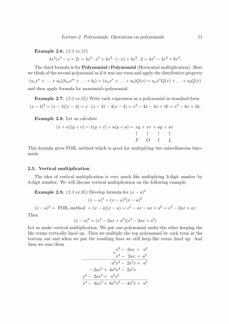
Let us make vertical multiplication. We put one polynomial under the other keeping thelike terms vertically lined up. Then we multiply the top polynomial by each term at thebottom one and when we put the resulting lines we still keep like terms lined up. Andthen we sum them

x2 − 2ax + a2

×x2 − 2ax + a2

a2x2 − 2a3x+ a4

− 2ax3 + 4a2x2 − 2a3x

x4 − 2ax3 + a2x2

x4 − 4ax3 + 6a2x2 − 4a3x+ a4


Example 2.10. (2.3 ex.97 ) Explain why the degree of the product of two polynomialsequals the sum of their degrees?

Lecture 3.

Factoring polynomials

The factoring is an operation inverse to the multiplication. When factored, a polynomial ismuch easier to understand and its properties are more obvious. We will consider general proce-dure for factoring polynomials of the second degree and some examples of factoring polynomialsof polynomials of higher degree.

3.1. Factoring

The factoring is the process inverse to the multiplication. Consider the followingmultiplication formulas (see page 77 (SMS))

(x− a)(x+ a) = x2 − a2,

(x+ a)(x+ a) = x2 + 2ax+ a2,

(x− a)(x− a) = x2 − 2ax+ a2.

Let us read these expressions from the right to the left. The right sides of these equationsare polynomials in standard form in the left sides the same polynomials are presentedas products of other polynomials. The polynomials standing in the left side are calledfactors.

Definition 3.1. Expressing a given polynomial as a product of other polynomials,that is, finding the factors of a polynomial is called factoring.

If a polynomial cannot be written as the product of two other polynomials (excludingconstants) then the polynomial is said to be prime.

When a polynomial has been written as a product consisting only of prime factors,then it is said to be factored completely.

Examples of prime polynomials are a) constants: 3,√

2, π; b) polynomials of degree 1:(x+ const); c)some quadratic polynomials: (x2 + x+ 1), (x2 + 1) (quadratic polynomialswith no real roots).

Unfortunately, there is no general procedure how to factor polynomial of an arbitrarydegree. It can be done for the polynomials of second and third degree, but in other casesone has to apply some insight. Some simple techniques we will discuss now.

Lecture 3. Factoring polynomials 14

3.2. Factoring out common multiplier

The instructive idea can be to factor out the common multiplier:

ab+ ac = a(b+ c).

Let us look at the examples.

Example 3.1. Factor the polynomials completely: (2.4 ex.5 )

x3 + x2 + x = x(x2 + x+ 1);

(2.4 ex.9 )3x2y − 6xy2 + 12xy = 3xy(x− 2y + 4).

3.3. Using special factoring formulas

Special factoring formulas are nothing but the product formulas written forward back-ward (see page 77 (SMS)).

x2 − a2 = (x− a)(x+ a),

x2 + 2ax+ a2 = (x+ a)(x+ a),

x2 − 2ax+ a2 = (x− a)(x− a),

x3 + a3 = (x+ a)(x2 − xa+ a2),

x3 − a3 = (x− a)(x2 + xa+ a2).

Example 3.2. Factor the polynomials completely. (2.4 ex.48 )

x8 − x5 = x5(x3 − 1) = x5(x− 1)(x2 + x+ 1).

(2.4 ex.57 )

16x4 − 1 = (4x2)2 − 1 = (4x2 − 1)(4x2 + 1) = (2x+ 1)(2x− 1)(4x2 + 1)

(2.5 ex.68 )8x4 − 18x2 = 2x2(4x2 − 9) = 2x2(2x+ 3)(2x− 3).

3.4. Factoring second-degree Polynomials. Factoring over integer numbers

For the second degree polynomial there is a bunch of techniques which solves theproblem of factoring completely. Consider a second degree polynomial that have a leadingcoefficient 1. Suppose we can factor this polynomial completely

(x2 +Bx+ C) = (x+ u)(x+ v) = x2 + (u+ v)x+ uv


If the factoring is possible then a and b should satisfy

(u+ v) = B, uv = C.

Now to factor the polynomial at second degree of the form

(x2 +Bx+ C)

consider C. Find out how C can be factored in u · v, this will give you a number ofcombinations. Then, check what combination meets u+ v = B.

Example 3.3. Factor the polynomials completely. (2.5 ex.4 )

x2 + 9x+ 8 : u · v = 8, u+ v = 9

8 = 4 · 2 = 1 · 8 = (−4) · (−2) = (−1) · (−8) = uv

The second combination meets u+ v = 9, therefore

x2 + 9x+ 8 = (x+ 1)(x+ 8).

(2.5 ex.65 )

x4 + 2x2 + 1 : y = x2 ⇒ y2 + 2y + 1 = (y + 1)2 ⇒ (x2 + 1)(x2 + 1).

Remark 3.1. You can not use this approach if a and b are not integers, moreovereven if a and b are integers, still u and v might be not integers and then it will be verydifficult to make a good guess for u and v.

3.5. Factoring second-degree Polynomials. Factoring over real numbers

Consider arbitrary polynomial of second degree.

ax2 + bx+ c

we will factor this polynomial completely using identities

(x+ a)(x+ a) = x2 + 2ax+ a2 and (x− a)(x+ a) = x2 − a2.

Step 1. Factor the coefficient a out to get

a(x2 +

b

ax+

c

a

).

Step 2. Complete full square for first two term using the first of two identities

a(x2 + 2

b

2ax+

c

a

)= a(x2 + 2

b

2a+( b

2a

)2

−( b

2a

)2

+c

a

)= a((x+

b

2a

)2

− b2

4a2+

4ac

4a2

)= a((x+

b

2a

)2

− b2 − 4ac

4a2

)= a((x+

b

2a

)2

− D4a2

),


where D = b2 − 4ac. When D ≥ 0 the last expression can be rewritten as

= a((x+

b

2a

)2

−(√D

2a

)2).

Step 3. Applying the second identity we factor this expression to get

= a(x+

b

2a−√D

2a

)(x+

b

2a+

√D

2a

)= a(x−

(−b+√D

2a

))(x−

(−b−√D2a

)).

This formula will work for arbitrary coefficients a, b, c, when D ≥ 0. If D < 0 thenfactoring is impossible in real numbers and the polynomial is prime.

Example 3.4. Factor the polynomial completely (2.5 ex.80)

(x5 − x3) + (8x2 − 8) = x3(x2 − 1) + 8(x2 − 1) = (x3 + 8)(x2 − 1)

= (x+ 2)(x2 − 2x+ 4)(x+ 1)(x− 1).

The second factor here is prime since D = (−2)2 − 4 · 1 · 4 = −12.

Lecture 4.

Rational expressions

A rational expression is an expression of the form when a polynomial is divided over apolynomial. In this lecture we will consider some basic approaches for simplifying rationalexpressions.

4.1. Division of polynomials

Definition 4.1. If P (x) is a polynomial of degree m Q(x) is a polynomial of degreen, and n < m then there exists a polynomial S(x) of degree m−n and a polynomial r(x)of degree < n such that

S(x) ·Q(x) + r(x) = P (x) orP (x)

Q(x)= S(x) +

r(x)

Q(x).

Here P (x) is called the dividend, Q(x) is called the divisor, S(x) is called the quotient,and r(x) is called the remainder.

The procedure of dividing polynomial over the polynomial is similar to procedure fordividing one integer over another integer. For integers we have a familiar formula. Ifb < a then there exists integer numbers q and r < b such that

qb+ r = a ⇔ a

b= q +

r

b.

Again, a is the dividend, b is the divisor, q is the quotient, and r is the remainder. Youcan check that the formulas remain the same for the polynomials.

The most popular technique for division of polynomials is similar to the long divisionof numbers

Lecture 4. Rational expressions 18

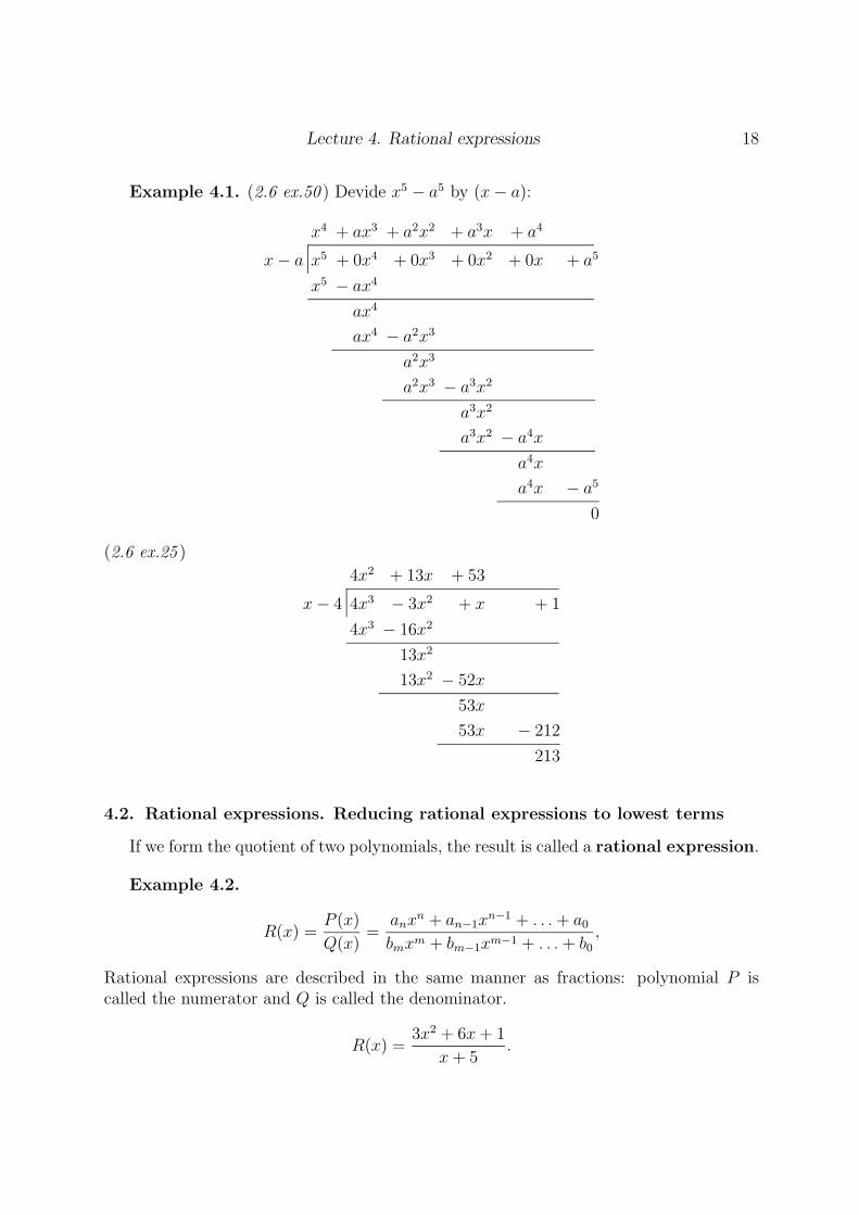
Example 4.1. (2.6 ex.50 ) Devide x5 − a5 by (x− a):

x4 + ax3 + a2x2 + a3x + a4

x− a x5 + 0x4 + 0x3 + 0x2 + 0x + a5

x5 − ax4

ax4

ax4 − a2x3

a2x3

a2x3 − a3x2

a3x2

a3x2 − a4x

a4x

a4x − a5

0

(2.6 ex.25 )

4x2 + 13x + 53

x− 4 4x3 − 3x2 + x + 1

4x3 − 16x2

13x2

13x2 − 52x

53x

53x − 212

213

4.2. Rational expressions. Reducing rational expressions to lowest terms

If we form the quotient of two polynomials, the result is called a rational expression.

Example 4.2.

R(x) =P (x)

Q(x)=

anxn + an−1x

n−1 + . . .+ a0

bmxm + bm−1xm−1 + . . .+ b0

,

Rational expressions are described in the same manner as fractions: polynomial P iscalled the numerator and Q is called the denominator.

R(x) =3x2 + 6x+ 1

x+ 5.


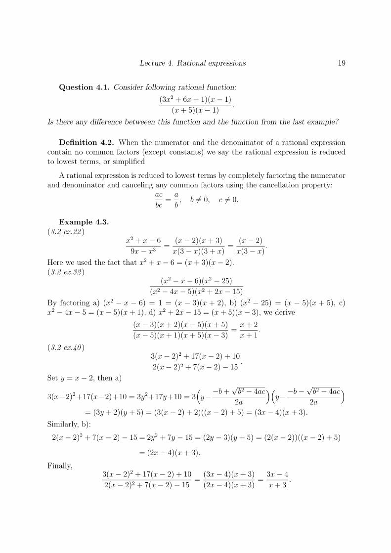
Question 4.1. Consider following rational function:

(3x2 + 6x+ 1)(x− 1)

(x+ 5)(x− 1).

Is there any difference betweeen this function and the function from the last example?

Definition 4.2. When the numerator and the denominator of a rational expressioncontain no common factors (except constants) we say the rational expression is reducedto lowest terms, or simplified

A rational expression is reduced to lowest terms by completely factoring the numeratorand denominator and canceling any common factors using the cancellation property:

ac

bc=a

b, b 6= 0, c 6= 0.

Example 4.3.(3.2 ex.22 )

x2 + x− 6

9x− x3=

(x− 2)(x+ 3)

x(3− x)(3 + x)=

(x− 2)

x(3− x).

Here we used the fact that x2 + x− 6 = (x+ 3)(x− 2).(3.2 ex.32 )

(x2 − x− 6)(x2 − 25)

(x2 − 4x− 5)(x2 + 2x− 15)

By factoring a) (x2 − x − 6) = 1 = (x − 3)(x + 2), b) (x2 − 25) = (x − 5)(x + 5), c)x2 − 4x− 5 = (x− 5)(x+ 1), d) x2 + 2x− 15 = (x+ 5)(x− 3), we derive

(x− 3)(x+ 2)(x− 5)(x+ 5)

(x− 5)(x+ 1)(x+ 5)(x− 3)=x+ 2

x+ 1.

(3.2 ex.40 )3(x− 2)2 + 17(x− 2) + 10

2(x− 2)2 + 7(x− 2)− 15.

Set y = x− 2, then a)

3(x−2)2+17(x−2)+10 = 3y2+17y+10 = 3(y−−b+

√b2 − 4ac

2a

)(y−−b−

√b2 − 4ac

2a

)= (3y + 2)(y + 5) = (3(x− 2) + 2)((x− 2) + 5) = (3x− 4)(x+ 3).

Similarly, b):

2(x− 2)2 + 7(x− 2)− 15 = 2y2 + 7y − 15 = (2y − 3)(y + 5) = (2(x− 2))((x− 2) + 5)

= (2x− 4)(x+ 3).

Finally,3(x− 2)2 + 17(x− 2) + 10

2(x− 2)2 + 7(x− 2)− 15=

(3x− 4)(x+ 3)

(2x− 4)(x+ 3)=

3x− 4

x+ 3.


4.3. Evaluating rational expressions

To succeessfuly evaluate a rational expression for some value of the variable we needto remember only one thing. The denominator can not be zero for that value. After thatwe have to evaluate the polynomial in the numerator, polynomial in the denominator andtake the ratio.

Example 4.4. (3.2 ex.50 ) Evaluate 5x2

1− x2 at x = 4.23

P (x) = 5x2 = 89.4645,

Q(x) = 1− x2 = −16.8929,

P

Q= −5.2960.

(3.2 ex.58 ) Determine which of the values must be excluded from the domain of thevariable in rational expression: a) x = 3, b) x = 1, c) x = 0, d) x = −1,

9x2 − x+ 1

x2 + x=

−9x

x(x+ 1).

Answer: When x = 0 the denominator of the rational expression is zero, therefore x = 0should be excluded from the domain.

4.4. Multiplication and division of rational expressions

The rules for multiplication and division of rational expressions are the same as therules for multiplying and dividing fractions.

a

b· cd

=ac

bd,

1ab

=b

a,

abcd

=ad

bc.

Example 4.5. (3.3 ex.22 )

1− x1 + x

· x2 + x

x2 − x=

(1− x)(x2 + x)

(1 + x)(x2 − x)=

(1− x)(x)(x+ 1)

(1 + x)x(x− 1)= 1.

(3.3 ex.25 )

2x2 + x− 3

2x2 − x− 3· 4x2 − 9

x2 − 1=

(2x2 + x− 3)(4x2 − 9)

(2x2 − x− 3)(x2 − 1)=

(2x+ 3)(x− 1)(2x+ 3)(2x− 3)

(2x− 3)(x+ 1)(x− 1)(x+ 1)

=(2x+ 3)2

(x+ 1)2.


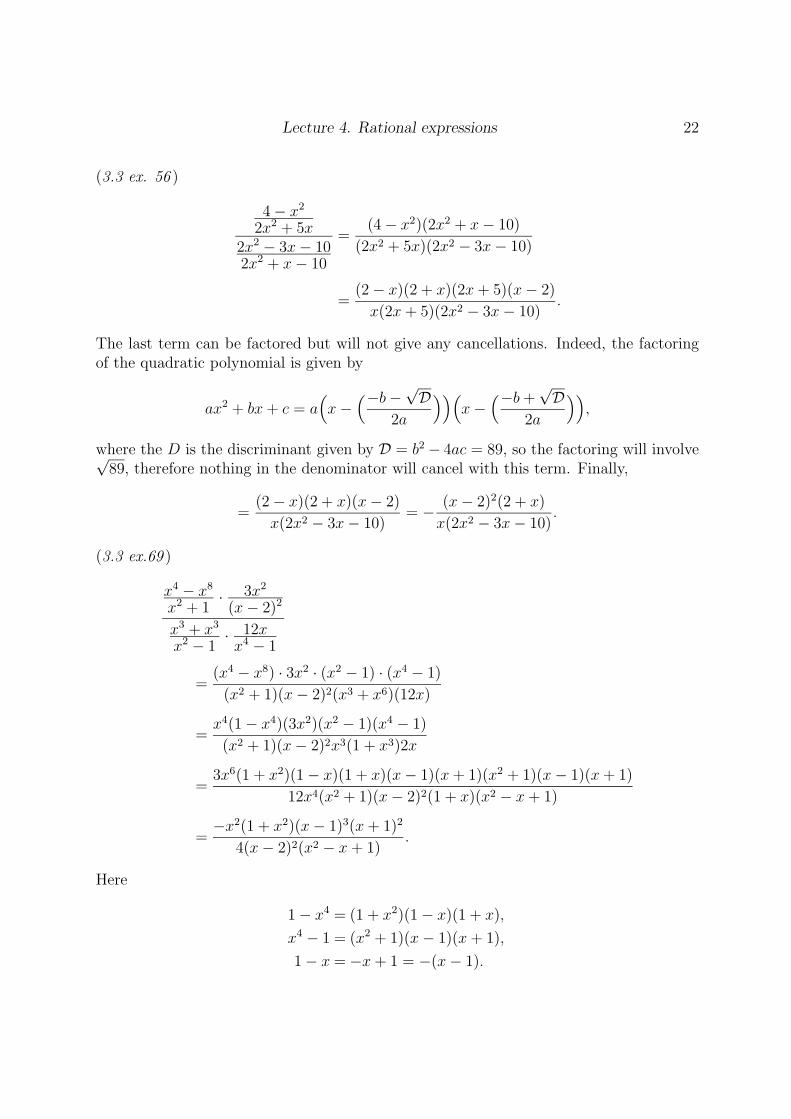
(3.3 ex. 56 )

4− x2

2x2 + 5x2x2 − 3x− 102x2 + x− 10

=(4− x2)(2x2 + x− 10)

(2x2 + 5x)(2x2 − 3x− 10)

=(2− x)(2 + x)(2x+ 5)(x− 2)

x(2x+ 5)(2x2 − 3x− 10).

The last term can be factored but will not give any cancellations. Indeed, the factoringof the quadratic polynomial is given by

ax2 + bx+ c = a(x−

(−b−√D2a

))(x−

(−b+√D

2a

)),

where the D is the discriminant given by D = b2 − 4ac = 89, so the factoring will involve√89, therefore nothing in the denominator will cancel with this term. Finally,

=(2− x)(2 + x)(x− 2)

x(2x2 − 3x− 10)= − (x− 2)2(2 + x)

x(2x2 − 3x− 10).

(3.3 ex.69 )

x4 − x8

x2 + 1· 3x2

(x− 2)2

x3 + x3

x2 − 1· 12xx4 − 1

=(x4 − x8) · 3x2 · (x2 − 1) · (x4 − 1)

(x2 + 1)(x− 2)2(x3 + x6)(12x)

=x4(1− x4)(3x2)(x2 − 1)(x4 − 1)

(x2 + 1)(x− 2)2x3(1 + x3)2x

=3x6(1 + x2)(1− x)(1 + x)(x− 1)(x+ 1)(x2 + 1)(x− 1)(x+ 1)

12x4(x2 + 1)(x− 2)2(1 + x)(x2 − x+ 1)

=−x2(1 + x2)(x− 1)3(x+ 1)2

4(x− 2)2(x2 − x+ 1).

Here

1− x4 = (1 + x2)(1− x)(1 + x),

x4 − 1 = (x2 + 1)(x− 1)(x+ 1),

1− x = −x+ 1 = −(x− 1).

real numbers. constants, variables, and mathematical …ama5348/umn2002f/math1051/lec1_4.pdf · y...

Documents