real power generation tracing for deregulated power … · (ann) and flower pollination (fpa). 2.1...

Journal of Theoretical and Applied Information Technology 30

th November 2015. Vol.81. No.3

© 2005 - 2015 JATIT & LLS. All rights reserved.

ISSN: 1992-8645 www.jatit.org E-ISSN: 1817-3195

564

REAL POWER GENERATION TRACING FOR

DEREGULATED POWER SYSTEM USING THE FLOWER

POLLINATION ALGORITHM TECHNIQUE

1S. H. M. KERTA,

2Z. A. HAMID,

3I. MUSIRIN

2Faculty of Electrical Engineering, Universiti Teknologi MARA, Malaysia

E-mail: [email protected],

[email protected]

ABSTRACT

In deregulated power market, providing a fair and non-discriminatory service pricing is still in debate on

‘who should be blame’ for the losses contribution. The use of traditional methods such as postage stamp

and MW mile methodology is said to be unreliable and biasing because of neglecting the power flow and

physical constraints. Thus, a new theory called electricity tracing has been developed to solve the problem

concerning non-discriminatory tranmission service pricing. The most common methods used are

Proportional Sharing Principle (PSP) and Superposition Theorem (ST). However, due to necessity of

matrix inversion and singularity of matrix in the mathematical equation, it is likely an error will occur and

result in unsatisfactory outputs. To explore a new method, this paper demonstrates an Artificial Intelligence

(AI) based optimization method, that is, Flower Pollination Algorithm (FPA) to perform real power

generation tracing. The experiment and comparative studies on IEEE-14 bus power system have verified

the capability of the proposed method for real system application with promising results.

Keywords: FPA, Generation Tracing, Losses Allocation, Matrix Inversion, Proportional Sharing Principle

1. INTRODUCTION

Nowadays, the electrical power industry is

shifted from monopolistic vertical structure to a

deregulated market structure. The deregulated

market consists of four main player, the

independent service provider (ISO), the

transmission companies (TRANSCO), the

generation companies (GENCO) and the

distribution companies (DISCO). Hence, the

allocation charges among this players must be made

fully fair and transparent [1]. The introduction of

deregulated market in countries like New Zealand,

Australia and a few regions in Canada, is an

approach to increase the efficiency in operation and

at the same time to reduce the energy price [2].

Perhaps, Scandinavia countries are the most

established in deregulated market [3]. Nevertheless,

allocation charge for generators and loads is

complicated to be performed since it is hard to trace

from which power of generators or loads

contributed to each transmission lines on certain

bus. Since then, there are various methods to

allocate the charges introduced by researches: the

MW mile method, contract path method and

postage stamp allocation [4]. In the case of power

scheduling, article [5] has explored the optimal

control theory technique called Maximum

Principle. This technique validates whether the

power scheduling is feasible for penalty charged to

GENCOs. For spot market price, the optimal

bidding and contracting strategy has been explored

in [6] for providing a free risk trade among

GENCO and DISCO under the specific merits.

There are many other methods of charge allocation

available for deregulated power market [7].

However, none of the mentioned methods give

satisfactory results. This problem has already

attracted many researchers to find a new solution

for effective and transparent allocation of losses

charge. The outcome of studies has brought to the

emergence of a new method called power tracing.

The advantage of tracing method is that the method

take account of the physical power flow constraints

and able to trace the power contributed by

generators or loads [8].

Power tracing has two primary studies namely

the generation tracing and load tracing. Generation

tracing traces the power contributed by generators,

while load tracing traces the power contributed by





565

loads. Thus, the algorithm based on Proportional

Sharing Principle (PSP) was proposed by Bialek in

[9] and [10]. The technique is based on Topological

Generator and Load Distribution Factor (TGLDF)

and the element of the technique consists of

upstream and downstream algorithm. TGLDF

frequently uses a large matrix inversion in

mathematical equation. However, the power system

need to be assumed lossless in transmission lines

which leads the tracing results less accurate.

Kirschen method make an extension in PSP by

organizing each loads and buses into homogeneous

group [11]. The concept of domain generator,

common and link have also been introduced for

power tracing. Meanwhile, Dai et al has developed

the power tracing for reactive power and it is

proven to be suitable for large system [12].

Nevertheless, Kirschen and Dai techniques are still

based on PSP and this has made both techniques

carried the same weakness as in TGLDF method.

Later, the Superposition Theorem (ST) was

proposed by Teng [13]. The technique used a

circuit theory in the tracing algorithm and it is able

to trace the voltages, current, real and reactive

power from both generators and loads

simultaneously. However, the existence of negative

sharing in the tracing results is unable to be defined

and leads to confusions. Afterward, the tracing

power using prediction based algorithm such as

Artificial Neural Network (ANN) was exploited by

[14] and [15]. The ANN is proven to have a robust

tracing process but the characteristic of tracing

results has no uniqueness since the training data

rely on the existing power tracing techniques.

Article [16] has proposed power tracing via SVC,

which is extension studies on prediction of the

manner of reactive power in the deregulated

market. Later, a hybrid method has been developed

by Shareef and Mustafa in [17] by combining the

existing power tracing method such as Common,

Node and Graph method. However, due to the

complexity of power tracing and a lot of

assumptions have to be considered, the method

became less attractive as it is easy for an error to

occur in the tracing results. After that, article [18]

has proposed a power tracing using optimization

method and the primary elements for control

variables, constraint and objective function are

specified accordingly. The proposed method

successfully created the algorithm which is free

from matrix inversion and assumptions such as

PSP. In article [19], the optimization technique

using Genetic Algorithm has been explored for

power tracing. Later, the article [20] has

successfully implemented Evolutionary

Programming which satisfies the power system

constraints. Recently, the article [21] has proven

that the use of Artificial Bee Colony (ABC) is far

more superior than the Particle Swarm

Optimization (PSO) technique in terms of

computation time and the accuracy of tracing

results. On overall, these reviews have motivated

the authors to conduct a study on electricity tracing

by means of different approach.

This paper proposes a bio-inspired optimization

algorithm by means of Flower Pollination

Algorithm (FPA) which is developed by Yang [22].

It was reported that the FPA techniques offers a

good computation time, robust in finding the best

solution and simplicity. In article [23], FPA

technique is able to perform good optimization

considering continuous domain. To establish the

algorithm equations, FPA requires only small

number of parameters which makes it an easier tool

to be implemented for optimization problem [24].

In fact, the key mechanism of exploration and

exploitation embedded within FPA algorithm

namely global and local pollination, allows for

effective optimization in the searching space. In

articles [25], the author has proven that the FPA is

better as compared to Bat algorithm (BA).

Therefore, the above reviews have motivated this

research to apply power tracing via FPA

techniques. The developed technique will be

applied in IEEE 14-bus test system concerning real

power generation tracing. The performance of the

proposed tracing algorithm will be compared with

other methods.

2. METHODOLOGY

In this section, two conventional power tracing

algorithms are presented: Topological Generator

and Load Distribution Factor (TGLDF) and

Superposition Technique (ST) as proposed by [9]

and [13] respectively. Besides that, two Artificial

Intelligence algorithms for power tracing will be

described, namely the Artificial Neural Network

(ANN) and Flower Pollination (FPA).

2.1 Conventional Power Tracing

Conventional power tracing is strictly based on

matrix operation and derivation. For the purpose of

this paper, two conventional power tracing

algorithms namely the TGLDF and ST are

explained as follows:

A) Topological Generation & Load Distribution

Factor





566

This method was proposed by J. Bialek [9]. The

method assumes that the power flow through a node

will be proportionally shared through all path that

bring outflows from that node.

This principle was developed to find the usage

capacity of generator and load via upstream and

downstream algorithm. When looking the tracing at

the nodal balance of inflow (upstream looking

algorithm), the total power through each node, Pi

can be expressed as:

(1)

Equation (1) shows that the power contribution

from each Pgk through a node is equal to |Au-1

|.Pgk;

where, Au is n x n upstream distribution matrix and

(i, j) element of Au is equal to:

∈−=−

=

=−

otherwise;0

for;||

for;1

][ )(α Ui

j

ijijiju

P

Pc

ji

A

(2)

Where Pj represent power through bus j, Pj-i

represent the line flow into line j-i , and αi(u)

is the

sets of nodes supplying directly to bus i .

Therefore, the line outflow of transmission line i-l

according to proportional sharing principle (PSP)

can be calculated as:

(3)

Similarly, the load demand PL-i can be calculated as:

(4)

The equation is useful to find where the

contributor’s power for a certain load comes from.

B) Superposition method

This method was proposed by Teng [13]. The

method is developed based on circuit theories,

equivalent current injection and equivalent

impedance. Firstly, the converged power flow

results has to be obtained in order to find the power

injections, bus voltage angles, bus voltage

magnitudes and power flows at both ends of a line.

After that, the complex power injection, Sn,G of a

generator bus n can be expressed as:

(5)

Where, Pn,G and Qn,G are real and reactive power

injection at n-th generator bus respectively.

Then, the following equations are used to

determine the equivalent current injection of

generator and equivalent impedance of load. The

corresponding equivalent current injection of

generator, In,G is:

(6)

Where, Vn,G is the voltage at n-th generator bus

obtained from the converged power flow solution.

Next, the corresponding equivalent impedance of

load, Zi,L is:

(7)

Where, Vi,L , Ii,,L and Si,L = Pi,L + jQi,L are the voltage,

current and power of load at i-th bus obtained from

the converged power flow solution.

After the equivalent impedance was integrated

into the admittance matrix, the relationship between

bus voltages and bus current injections can be

formed into a transmission system with N buses as

follows:

=

=

∆

∆

∆

0

0

,

1

1

11111

M

M

LLL

MOLOM

LL

MLLLM

LL

M

M

I

ZZ

ZZZ

ZZZ

NV

nV

V

Gn

NNN

nNnnn

Nn

n

n

n

(8)

Equation (8) shows that the voltage at bus i

contributed by generator at bus n (i.e. ∆Vi n) can be

written as:

(9)

gk

n

kiku

i

lii

i

lili PA

P

PP

P

PP ⋅=⋅= ∑

=

−−−−

1

1][

gk

n

kiku

i

iLi

i

iLiL PA

P

PP

P

PP ⋅=⋅= ∑

=

−−−−

1

1][

niPAPn

kgkui ,...,2,1for;][

1

1 == ∑=

−

jQPS GnGnGn ,,, +=

*

,

,,,

+=

Gn

GnGnGn

V

jQPI

LiLi

Li

Li

LiLi

jQP

V

I

VZ

,,

2

,

,

,, −

==

Gninn

i IzV ,∗=∆





567

And the voltage of bus i contributed by all

generators will be:

(10)

Next, to determine the contributed current by any

particular generator, the following figure needs to be

considered.

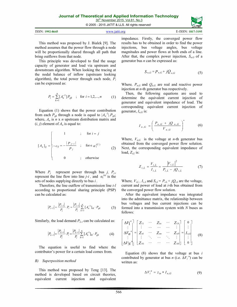
Fig. 1. A transmission line section model

The line current between buses i and j

corresponding to the voltage contributed by

generator bus can be expressed as:

(10a)

(10b)

Where, yij = gij + jbij is the line admittance from bus

i to j and c/2 is the line charging susceptance.

Thus, Δiijn and Δiji

n are the line currents from bus

i to bus j and bus j to bus i respectively, contributed

by generator at bus n. Therefore, the total line

current from bus i to j is expressed as:

(11)

Since the voltage and current can be identified,

the complex power flow, Sij from bus i to j can be

expressed as:

(12)

(13)

From the equation (13), the complex power flow

contributed by generator at bus n is given as:

(14)

And the complex power loss on the line between

bus i and j can be expressed as:

(15)

Lastly, the real power loss contributed by

generator at bus n can be expressed as:

(16)

Thus, the total line losses in any particular line

can be expressed as:

(17)

In summary, this tracing method has 4 essential

steps which are the tracing of voltages, current,

power flow and losses through equations (10), (11),

(15) and (17) sequentially.

2.2 Artificial Intelligence Method

In this section, the method of power tracing via

Artificial Intelligence (AI) will be explained

briefly. The AI has an important role in solving

complex mathematical problem. The power tracing

has benefits in using AI method as its solver.

Recently, there are numerous studies on how to

solve power tracing problem via AI approaches.

The commonly used method is the Artificial Neural

Network (ANN) and Optimization method. The

ANN is a supervised learning inspired from the

biological neurons and suitable for forecasting and

predicting future data. The optimization method is a

process to find the best solution inspired by nature

movement likes flocking of birds, bacteria and ant

colony. The AI approaches have proven to be less

computational burden and easy to be implemented.

The following subsections will explain in brief on

the methodology involving AI methods.

∑=∆=

GN

n

nii VV

1

( ) ( )in

ijijjn

in

ijn

V2

jcjbgVVi ∆

+

∆−∆=∆

( )

∆

+

∆−∆=∆ j

nijiji

njn

jin

V2

jcjbgVVi

*

11

*)(

∆

∆== ∑∑

==

GG N

n

nij

N

n

niijiij ivIVS

∑ ∆==

GN

1n

nijij iI

∑ ∆==

GN

1n

nLoss,ijLoss,ij PP

( )( )GG

GG

Nij

Nijijij

Ni

Niiiij

iiii

vvvvS

∆+∆++∆+∆∗

∗∆+∆++∆+∆=

−

−

121

121

...

...

K

K

∑ ∆==

GN

1n

nijLoss,ij sS

*)( niji

nij iVs ∆=∆

( ) ( )nji

nij

nlossij ssP ∆+∆=∆ ReRe,





568

A) Artificial Neural Network (ANN)

The ANN consists of three basic layers; input,

output and hidden layer. Each layer has a number of

nodes and connected between each layer. This

connection is represented by weighted input data

[26]. In addition, the ANN performs two major

tasks; namely the training and testing. Training is

the process of adapting the data to produce the

desired output and to be presented as input memory.

If the desired output data is unsatisfactory, the ANN

complexity need to be increased such as creating

more connection between weights input data. In

contrast, testing is the integral part of training

process and create response at the output memory.

In relation to the power tracing, the input training

data is acquired from the conventional power tracing

methods such as TGLDF or Superposition theorem.

The input will be connected to a number of layers in

the systems to produce a desired output. Various

techniques have been introduced using other

methods to be represented as the input training data

such as in [14] and [15]. Above all, the training data

will be tested to create a response from output

memory and if the ANN testing failed to satisfy the

desired output, the training data need to be increased

until the satisfactory results are successfully

achieved. Nevertheless, the performance of power

tracing using ANN is still based on the results from

conventional power tracing. Hence, there is no

uniqueness in the tracing results. The process of

power tracing using ANN is illustrated in Fig. 2.

B) Optimization method

Optimization approach has been explored by [18].

The basic elements of the method consist of control

variable, constraint and objective function. The

control variable must not violate the specified

constraints in order that the objective function can

be maximized or minimized. The process to find the

best solution under the guidance of objective

function will determine the effectiveness and

robustness of the algorithm. In applying the

optimization approach, researchers have proven that

the method is simple in calculation without

complexity of mathematical formulation and

provide fairness for losses charge allocation. In

virtues of that, this paper intends to exploit the

benefits of optimization techniques through the

application of the Flower Pollination Algorithm

(FPA).

Fig 2. ANN Algorithm Assisted Power Tracing

2.3 Real power tracing concept

Since the topic of this paper will involve the real

power contributed by generators, it is necessary to

derive the mathematical relationship for generator’s

contribution in losses, line flows and load powers

before formulating it into FPA. In [18], the

contribution of generators of power Pgk in line

flows, Pflk and load, PLi

k is given as:

(18)

(19)

Here, xflk is the power flow fraction of l-th line

and xLik is the load power fraction of i-th load

contributed by k-th generator respectively. More

importantly, the equation (18) and (19) can be

defined as the percentage of a generator’s output

power used by a specific transmission line and load

in the system. The summation of generator

contribution in line flow of l-th line is expressed as:

(20)

gkkfl

kfl P.xP =

gkkLi

kLi P.xP =

ngen

flflflfl PPPP +++= ...21





569

Substituting (18) into (20):

(21)

(22)

Meanwhile, the generator contribution in i-th

load can also be described as:

(23)

Where, the term ‘ngen’ as in (22) and (23)

represents the number of generators in the system.

Both equations will be the equality constraints to

ensure no violation caused by FPA during

optimization process.

2.4 The Proposed Power Tracing Method

This section explains briefly the methodology of

power tracing via FPA. The FPA is a bio-inspired

algorithm in which has been evolving around 125

million years by the transfer of pollen using wind,

insect, bird and other animals [22]. The pollen is

carried in two ways, namely biotic and abiotic. In

biotic pollination, the insects and animals carry the

pollen to the stigma. While in abiotic pollination,

wind or diffusion in water is the tools for the

pollination. According to the survey in [25], 90% of

pollination takes biotic pollination process which

requires an animal and insects to be the pollinators.

By a close look into the pollination, there are two

methods of pollination, cross-pollination and self-

pollination.

Cross-pollination is a process of pollination from

a pollen of a flower of a different plant. By contrary,

self-pollination is the pollination of a flower, from

pollen of the same flowers or different flowers of

the same plant, which often happens when there is

no available pollinator. Biotic, cross-pollination may

be happened in long distance. Bees, bats, birds and

flies are mostly used as pollinators which are able to

fly for a long distance which obeying the Levy

distribution. So, these pollinators are considered as

the carrier of the global pollination. In addition,

there is a pollinator such as bees which tend to visit

exclusive certain flower species while bypassing

other flower species. This is known as flower

constancy which has the advantages to maximize

the transfer of pollen to the same species of flower,

hence, maximizing the reproduction of the same

flower species [22] – [25]. The objective of flower

pollination is to ensure the survival of the fittest and

the optimal reproduction of plants in terms of

number as well as the fittest [22]. This section will

discuss briefly the process of FPA in accordance to

the power tracing.

A) The Philosophy of FPA

The FPA as invented by Yang [22] is to be

implemented in the power tracing algorithm. To

understand the concept of FPA, there are primary

processes involved namely the biotic and abiotic

pollination, local and global pollination. For

simplicity, the essential processes are summarized

as follows:

1. Rule 1 – Biotic and cross-pollination can be

considered as a process of global pollination,

and pollen-carrying pollinators move in a way

which obeys Levy flights.

2. Rule 2 – For local pollination, abiotic

pollination and self-pollination are used.

3. Rule 3 – Pollinators such as insects can

develop flower constancy, which is equivalent

to a reproduction probability that is

proportional to the similarity of two flowers

involved.

4. Rule 4 – The interaction or switching of local

pollination and global pollination can be

controlled by a switch probability p ϵ [0; 1],

slightly biased towards local pollination.

B) Power Tracing using FPA

In this section, the FPA begins with initial

random number generation, evaluation of fitness,

production and selection of new generation. The

algorithm will take a longer computation time due to

a large pool of control variables; namely, the

number of generators, transmission lines and load

buses. If the formulation of algorithm is not done

properly, it will result in the burden of computation.

Therefore, the performance of programming is

essential to provide a good converged result of

optimization. The elements of algorithm such as

control variable, objective function, equality and

non-equality constraint will be set properly to give

proper guide for the algorithm. For the purpose of

this paper, the problem formulation was inspired by

the research conducted in [20], except for the type

of algorithm used to perform the optimization;

namely, the newly developed FPA. The appropriate

control variables, constraint and objective function

are explained below:

∑=

=ngen

kgk

kflfl PxP

1

.i.e

∑=

=ngen

k

gk

k

LiLi PxP1

.

ngeng

ngen

flgflgflfl PxPxPxP ,2

2

1

1 ...... +++=





570

i) Control Variable – The matrix X as in (24)

represents the individual candidates for FPA that

consists of contributed line flow and load power

fraction by k-th generator (i.e. xslk and xLi

k

respectively). Hence, xslk and xLi

k represent the

control variables in this algorithm. The order of

matrix X is given as (nbr + nload) x ngen, where

nbr, ngen, nload represent number of lines, number

of generators and number of loads respectively.

=

ngen

nloadL

k

nloadLnloadL

ngen

Li

k

LiLi

ngen

L

k

LL

ngen

L

k

LL

ngen

nbrs

k

nbrsnbrs

ngen

sl

k

slsl

ngen

s

k

ss

ngen

s

k

ss

xxx

xxx

xxx

xxx

xxx

xxx

xxx

xxx

,,

1

,

1

22

1

2

11

1

1

,,

1

,

1

22

1

2

11

1

1 ......

LL

MMM

MOMOM

LL

MMM

MOMOM

X

(24)

In fact, the line flow fraction consists of sending-

end power and receiving-end power. The sending-

end power fraction is chosen to be the control

variable since it comes directly from the generator

bus. Therefore, the receiving-end power and losses

fraction are calculated via (25) and (26) as follows:

(25)

(26)

Where, Psl and Prl represent the sending- and

receiving-end power of l-th line respectively. The

fraction xslk and xrl

k represent the sending- and

receiving-end power fraction of l-th line

respectively.

ii) Constraint – The FPA is subjected to some

considerable constraints to limit the searching

process. This is given as follows:

(27)

(28)

(29)

(30)

The constraint in (30) ensures that the contributed

fractions in matrix X are always in positive values

and does not exceed the corresponding generators

power. This will effectively enhance the accuracy of

tracing results.

iii) Objective function – The proposed objective

function was derived from power-balance equation.

This hypothetical equation should be utilized as the

fitness to guiding the searching of FPA. Firstly,

power generated by a generator should be equal to

the summation of total load power and losses

contributed by that generator. Mathematically:

(31)

The loss of l-th line contributed by a generator is

described by (32) as follows:

(32)

By substituting (23) and (32) into (31), the

following is obtained.

(33)

After simplification:

(34)

Rearrange (35):

(35)

Or:

(36)

∑∑==

+=nbr

l

k

lloss

nload

i

k

Ligk PPP1

,

1

ksl

sl

rlkrl

x.P

Px =

krl

ksl

kl,loss xxx −=

gk

k

lloss

k

lloss PxP .,, =

gk

nbr

l

klloss

nload

igk

kLigk PxPxP ..

1,

1

∑∑==

+=

∑∑==

+=nbr

l

klloss

nload

i

kLi xx

1,

1

1

011

,1

=−− ∑∑==

nbr

l

klloss

nload

i

kLi xx

∑∑==

−−=nbr

l

klloss

nload

i

kLigk xxE

1,

1

1)(min

∑=

=ngen

k

gk

k

slsl PxP1

.

∑=

=ngen

k

gk

k

rlrl PxP1

.

∑=

=ngen

k

gk

k

LiLi PxP1

.

1,,,0 , ≤≤ k

Li

k

lloss

k

rl

k

sl xxxx





571

Where, Egk is the generation-demand balance error

of k-th generator participated in the power tracing.

Hence, the objective of the algorithm is to minimize

the error Egk as low as possible.

C) Overall Algorithm for FPA-based-tracing

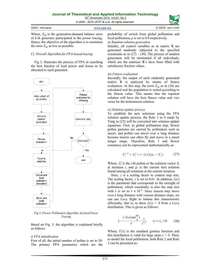
Fig 3. illustrates the process of FPA in searching

the best fraction of load power and losses to be

allocated to each generator.

Fig 3. Flower Pollination Algorithm Assisted Power

Tracing

Based on Fig. 3, the algorithm is explained briefly

as follows:

i) FPA initialization

First of all, the initial number of pollen is set to 50.

The primary FPA parameters which are the

probability of switch from global pollination and

local pollination, p is set to 0.8 respectively.

ii) Random solution generation

Initially, all control variables as in matrix X are

generated randomly subjected to the specified

constraints as in (27) – (30). The process of random

generation will be terminated if all individuals,

which are the matrices X’s have been filled with

satisfactory fraction values.

iii) Fitness evaluation

Secondly, the output of each randomly generated

matrix X is analyzed by means of fitness

evaluation. At this step, the error Egk as in (36) are

calculated and the population is sorted according to

the fitness value. This means that the topmost

solution will have the best fitness value and vice

versa for the bottommost solution.

iv) Solution update process

To establish the new solutions using the FPA

solution update process, the Rule 1 to 4 made by

Yang in [22] will be converted into solution update

equations. First, in global pollination step, flower

pollen gametes are carried by pollinators such as

insect, and pollen can travel over a long distance

because insects can often fly and move in a much

longer range. Therefore, Rule 1 and flower

constancy can be represented mathematically as:

(37)

Where, Xit is the i-th pollen or the solution vector Xi

at iteration t, and g* is the current best solution

found among all solutions at the current iteration.

Here, γ is a scaling factor to control step size.

The scaling factor, γ is set to 0.01. In addition, L(λ)

is the parameter that corresponds to the strength of

pollination, which essentially is also the step size

with λ is set to 1 x 10–6

. Since insects may move

over a long distance with various distance steps, we

can use Levy flight to imitate this characteristic

efficiently; that is, to draw L(λ) > 0 from a Levy

distribution. This is given as follows:

(38)

Where, Г(λ) is the standard gamma function and

this distribution is valid for large steps s > 0. Then,

to model the local pollination, both Rule 2 and Rule

3 can be presented as:

))(( *1 t

iti

ti XgLXX −⋅+=+ λγ

)0(1

)2

sin()(

~1

>>>⋅Γ⋅

+ osss

Lλπ

πλλλ





572

(39)

Where, Xit and Xj

t are pollen from different flowers

of the same plant species. This essentially imitates

the flower constancy in a limited neighborhood.

Mathematically, if Xit and Xj

t comes from the same

species or selected from the same population, this

equivalently becomes a local random walk if ε is

drawn from a uniform distribution in [0, 1]. In order

to mimic the switches of flower pollination for both

global and local, the switch probability, p is used

(Rule 4).

v) Assigning new generation

The selection of the offspring population (the new

population of matrix X) are evaluated via fitness

evaluation. Subsequently, both parents and

offspring population are combined and sorted

according to their quality of fitness; that is, the

highest solution represents the b-th matrix X with

the smallest error Egk among the population. The

last half of the combined population will be

discarded, while the first half will be assigned as

the new generation in the next iteration as if to

maintain the original population number.

vi) Convergence test

Eventually, the optimization will be terminated if

all matrices X’s have tolerable difference of fitness.

3. RESULT AND DISCUSSION

The developed algorithm was tested on IEEE 14-

bus power system for validation process. The power

system consists of 3 synchronous generators with 23

transmission lines for delivering MW power to

consumer, and 14 buses with 13 of them contain

loads. Although having numerous number of control

variables, the FPA algorithm requires about 52

seconds for searching process. This means that the

proposed algorithm was successful in providing

finite results. In this section, the proposed algorithm

was successfully tested for allocation of losses and

load power to generators. There are 2 competing

methods for the purpose of comparative study,

namely the Topological Generator and Load

Distribution Factor (TGLDF) and Superposition

Theorem (ST) as proposed in [9] and [13]

respectively. All the results in this section are

presented in the Appendices of this paper.

3.1 Allocation of losses to generators.

The generator contributions in losses using FPA,

TGLDF and ST are tabulated in Table A1, Table

A2 and Table A3 respectively.

It has been validated that the tracing results

produced by the algorithm satisfied the constraints

in equations (27) – (30). The total losses obtained

by using FPA are equal with that of the original

power flow results. Furthermore, there is no

negative sharing of losses obtained by using FPA

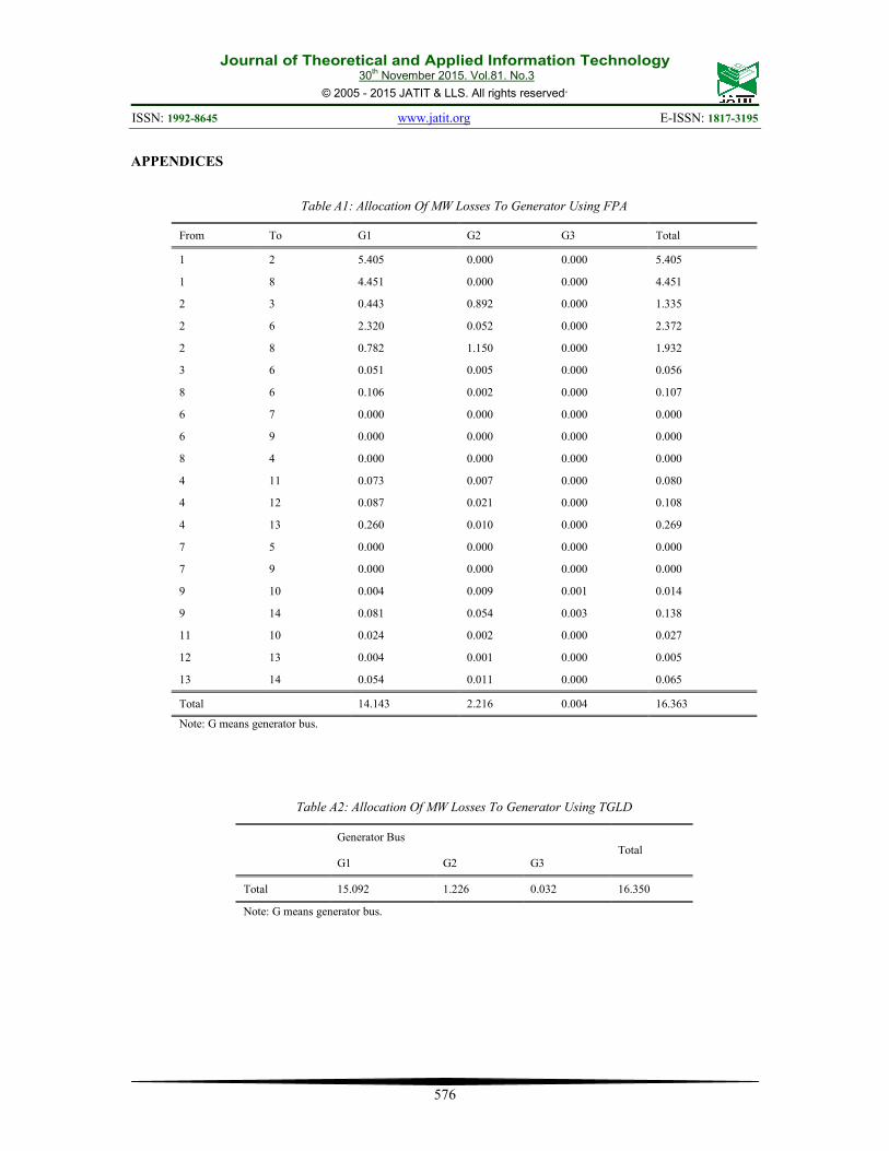
method. Based on Table A1, line losses from bus 9

to 14 contributed by generator G1, G2 and G3 are

0.081 MW, 0.054 MW and 0.003 MW respectively.

In addition, the total losses contributed by generator

G3 is 0.004 MW. This shows that, the losses

contributed by generator G3 using FPA is far

smaller than that of the TGLDF’s and ST which

result to 0.032 MW and 1.219 MW respectively.

In contrast to TGLDF’s method as in Table A2,

this method was unable to trace the individual

losses of each transmission line. As can be seen

from Table A2, the method indicates only total

losses contributed by each generator, which means

that it failed to detect which generators became the

major contributor for the losses in transmission

line. For example, the total real power losses is

16.35 MW and the total contributed losses by G1,

G2 and G3 are 15.092, 1.226 and 0.032 MW

respectively. This method involves a lot of

mathematical assumptions. For instance, the

method treat the line flow to be lossless and

perform the tracing process using 3 assumptions

according to [9]; namely, average line flow, gross

flows and net flows. As a result, this has lead to less

accuracy in tracing results. In addition, using the

large matrix inversion can lead to error in

calculation if the matrix is singular.

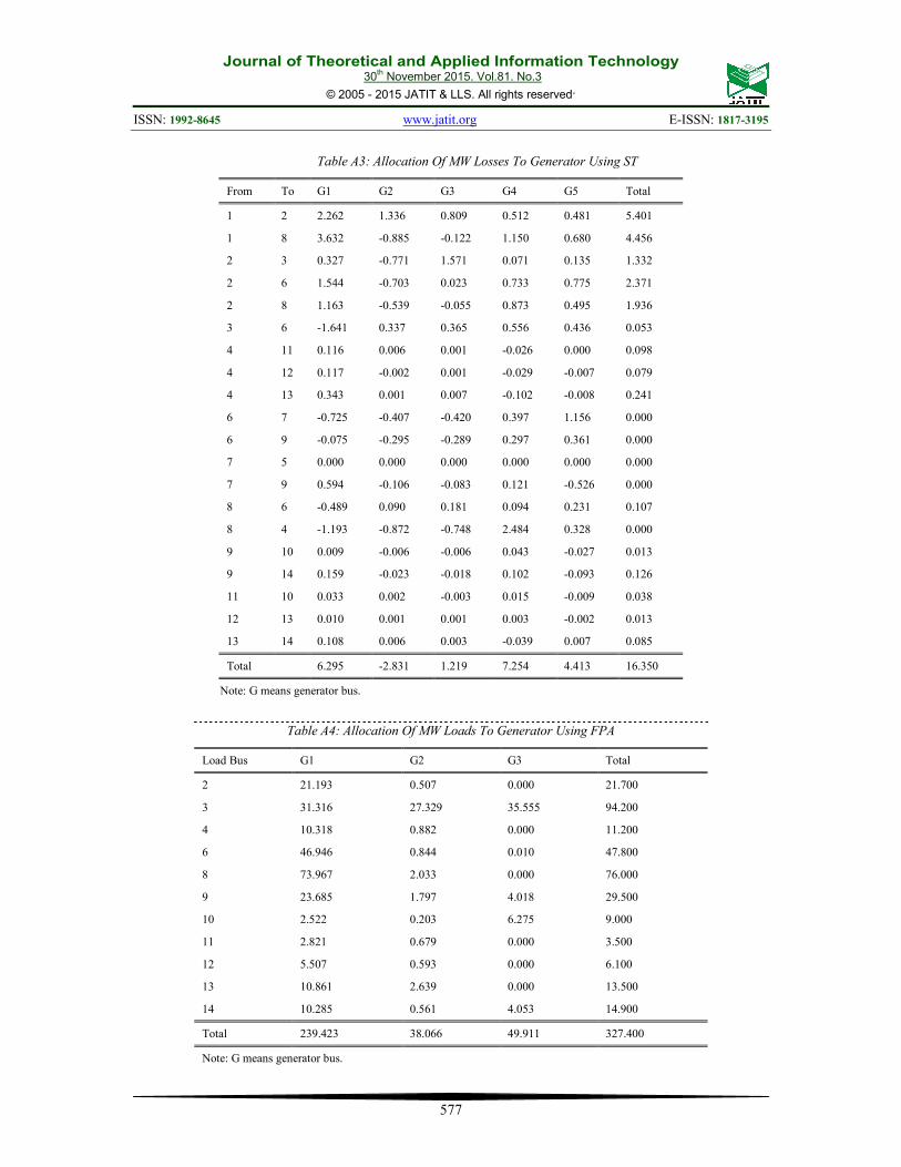
For ST method as in Table A3, it was successful

in resulting transparent result as that of FPA.

Through the method, the individual losses of each

transmission line was able to be traced and

allocated to generators. For example, from bus 1 to

bus 2, the line losses contributed by generators G1,

G2, G3, G4 and G5 are 2.262 MW, 1.336 MW,

0.809 MW, 0.512 MW and 0.482 MW respectively.

In addition, there is an increase in generators

participations in the losses contribution; where,

there are two synchronous condensers namely

generator G4 and G5 that also contribute the losses

to the system. However, synchronous condenser

which is frequently known as synchronous

capacitors in practical does not give any significant

contribution to the real power issues. The machine

acts as a stabilizer in transmission line and supplies

only reactive power to the system. Therefore, it is

illogical to say that synchronous condenser take

part in real power losses. In addition, the ST

method was unable to make the result of total losses

)(1 ti

tj

ti

ti XXXX −+=+ ε





573

free form negative contributions. For example in

Table A3, the losses in transmission lines from bus

8 to 4 contributed by generators G1, G2 and G3 are

-1.193 MW, -0.872 MW and -0.748 MW

respectively. Since there is no concrete reason for

the occurrence of negative sharing, it cannot be

accepted in the real power market as it introduces

confusing interpretation in the transmission service

pricing.

As a result, FPA method holds several

advantages compare to the conventional methods.

The FPA method has no mathematical assumptions;

hence, leads to more accuracy in results. There is

no large matrix inversion is required here. This can

minimize the error during computation process.

From here, the FPA method is proven to be easy for

implementation, robust for result accuracy and

efficient for optimization.

3.2 Generator contribution on MW loads

The generators contributions on MW loads using

FPA, TGLDF and ST are tabulated in Table A4,

Table A5 and Table A6 respectively.

By considering FPA in Table A4, the total load

power allocated to generator G1, G2 and G3 are

239.423 MW, 38.066 MW and 49.911 MW

respectively, while the result produced by TGLDF

as in Table A5 for G1, G2 and G3 are 253.75 MW,

40 MW and 50 MW respectively. For ST as in

Table A6, the total contributed load power by the

generators G1, G2 and G3 are 247.448 MW, 42.83

MW and 48.781 MW respectively. In addition,

based on ST there are additional generators namely

G4 and G5 that have contributed total load power

of -7.254 MW and -4.413 MW respectively. The

overall load power in the system resulted from

FPA, TGLDF and ST are 327.392 MW, 343.75

MW and 327.4 MW respectively.

As for TGLDF, the total MW loads is larger as

compared to ST and FPA. Nevertheless, there is no

much different on the result among the three

methods and it is acceptable for this case. For

TGLDF, the method makes several assumptions

such as proportional sharing principle and used a

matrix inversion for the calculation. As a result, the

total MW loads less accurate as compared to the

FPA. For ST, the assumptions need to be

undertaken are by transforming the generator bus as

an equivalent current injection and load bus as

equivalent impedance. Only when the impedance

matrix is non-singular, the tracing results can be

acquired. However, the existence of negative

sharing makes it less accurate.

From here, FPA holds several advantages as

compared to other methods. For instance, the FPA

is free from any assumptions and no matrix

singularity need to be accounted for calculation.

This has given the FPA more flexibility and

efficiency in terms of performance.

3.3 Comparison optimization method with

proposed method

The results for performance of FPA, EP and

ACOR are tabulated in Table 1. The comparative

study will be focused on the required time for

convergence and the optimal error, Egk resulted

from each algorithm.

Table 1: Performance of algorithm after optimization

Methods Convergence Time (sec)

Optimal error, Egk .

FPA 52 1.059 x 10-3

EP 176 5.59 x 10-5

ACOR 420 4.189 x 10-5

The FPA results in a finite computation time in

searching for optimal error, Egk. Based on the

results tabulated in Table 1, the time taken for FPA,

EP and ACOR to converge are 52, 176 and 420

seconds respectively. This entails that the FPA

method shows an excellent computation speed over

the others. While EP is average in computation

time, the ACOR takes longer time for searching the

best solution. In addition, it is obvious that FPA

results in tolerable error value as that of EP and

ACOR. Based on Table 1, although the error value

produced by ACOR is the lowest, the error value of

1.059 x 10-3

resulted from FPA is still satisfactory.

Based on these findings, EP and ACOR reflect their

merit only in the context of solution optimality, but

unable to promise fast optimization. Hence, FPA

offers a better optimization scheme as it has given a

satisfactory solution with promising speed

concurrently.

4. CONCLUSION

This paper has proven that the power tracing

technique using FPA is able to give satisfactory

results as compared to other conventional methods.

The FPA method successfully produced accurate

results for MW loads and losses contribution in 14-

bus power system without any assumptions, free

from matrix inversion and independent of matrix

singularity. As compared to others, the FPA was

able to give a tolerable searching mechanism with

minimum error and fast computation time. More

importantly, the proposed method was able to





574

maintain its simplicity regardless of the size of

power system and constraints. On overall, the

comparative studies have verified the competency

and capability of the proposed method for

deregulated market environment. For future

recommendation, the proposed method will be run

in larger test systems such as 57-bus power

systems.

ACKNOWLEDGEMENT

The authors would like to acknowledge The

Research Management Institute (RMI) of UiTM and

Ministry of Higher Education Malaysia (MOHE) for

the financial support via the Research Acculturation

Grant Scheme (RAGS) with project code: 600-

RMI/RAGS 5/3 (189/2014).

REFERENCES

[1] M. Shahidehpour, H. Yamin, and Z. Li,

“Market Operations in Electric Power

Systems : Forecasting, Scheduling, and Risk

Management,” Wiley and Sons Inc.

Publication, 2002.

[2] M. W. Mustafa and M. H. Sulaiman,

“Transmission Loss Allocation in Deregulated

Power System via Superposition and

Proportional Tree Methods,” 2nd IEEE Int.

Conf. Power Energy (PECon 08), December

1-3, 2008, Johor Baharu, Malaysia, vol. 3, pp.

988–993, 2008.

[3] A. Mazer,”Electric Power Planning for

Regulated Markets.” Wiley and Sons Inc.

Publication

[4] Z. Hamid, I. Musirin, M. M. Othman, and M.

N. a Rahim, “Comparative studies between

various power tracing techniques for reactive

power allocation,” ICCAIE 2011 - 2011 IEEE

Conf. Comput. Appl. Ind. Electron., no.

Iccaie, pp. 96–101, 2011.

[5] X. G. X. Guan, F. G. F. Gao, and a. Svoboda,

“Energy delivery capacity and generation

scheduling in the deregulated electric power

market,” Proc. 21st Int. Conf. Power Ind.

Comput. Appl. Connect. Util. PICA 99. To

Millenn. Beyond (Cat. No.99CH36351), pp.

25–30, 1999.

[6] D. J. Wu, P. Kleindorfer, and J. E. Zhang,

“Optimal Bidding and Contracting Strategies

in the Deregulated Electric Power Market :

Part II,” Proceeding 34th Hawaii Int. Conf.

Syst. Sci., no. IEEE, pp. 1–10, 2001.

[7] O. Pop, C. Barbulescu, P. Andea, D. Jigoria-

Oprea, F. Coroiu, and O. Tirian, “ComParison

of power system tracing cost allocation

methods,” EUROCON 2011 - Int. Conf.

Comput. as a Tool - Jt. with Conftele 2011,

no. 1, pp. 1–4, 2011.

[8] Z. M. Z. Ming, S. L. S. Liying, L. G. L.

Gengyin, and Y. N. Y. Ni, “A novel power

flow tracing approach considering power

losses,” 2004 IEEE Int. Conf. Electr. Util.

Deregulation, Restruct. Power Technol. Proc,

vol. 1, pp. 355–359, 2004.

[9] J. Bialek and P. A. Kattuman, “Proportional

Sharing Assumption in Tracing

Methodology,” IEE Proceedings-Generation,

Transm, vol. 151, no. 4, pp. 527–532, 2004.

[10] J. Bialek, “Topological generation and load

distribution factors for supplement charge

allocation in transmission open access,” IEEE

Trans. Power Syst., vol. 12, no. 3, pp. 1185–

1193, 1997.

[11] D. K. Ron and A. G. Strbac, “Contributions of

individual generators to loads and flows,”

IEEE Trans. Power Syst., vol. 12, no. 1, pp.

52–60, 1997.

[12] Y. Dai, X. D. Liu, Y. X. Ni, F. S. Wen, Z. X.

Han, C. M. Shen, and F. F. Wu, “A cost

allocation method for reactive power service

based on power flow tracing,” Electr. Power

Syst. Res., vol. 64, no. 1, pp. 59–65, 2003.

[13] J. H. Teng, “Power flow and loss allocation

for deregulated transmission systems,” Int. J.

Electr. Power Energy Syst., vol. 27, no. 4, pp.

327–333, 2005.

[14] M. W. Mustafa, A. B. Khairuddin, H. Shareef,

and S. N. A. Khalid, “Identification of Source

to Sink Relationship in Deregulated Power

Systems Using Artificial Neural Network,”

8th Int. Power Eng. Conf. (IPEC 2007), pp. 6–

11, 2007.

[15] M. De, N. B. D. Choudhury, and S. K.

Goswami, “Transaction based power flow

solution and transmission loss allocation using

neural network,” Power Electron. Drives

Energy Syst. & 2010 Power India, 2010

Jt. Int. Conf., 2010.

[16] M. Mandal and A. Chakrabarti, “Reactive

Power Tracing of a Multibus Power System in

Presence of SVC,” International Conference

on Control, Instrumentation, Energy &

Communication, pp. 254–258, 2014.

[17] H. Shareef and M. W. Mustafa, “A Hybrid

Power Transfer Allocation Approach for

Deregulated Power Sytems,” First Int. Power

Energy Conf. (PECon 2006), pp. 215–219,

2006.





575

[18] A. R. Abhyankar, S. A. Soman, and S. A.

Khaparde, “Optimization approach to real

power tracing: An application to transmission

fixed cost allocation,” IEEE Trans. Power

Syst., vol. 21, no. 3, pp. 1350–1361, 2006.

[19] M. H. Sulaiman, M. W. Mustafa, and O.

Aliman, “Transmission loss and load flow

allocations via genetic algorithm technique

BT - 2009 IEEE Region 10 Conference,

TENCON 2009, November 23, 2009 -

November 26, 2009,” pp. 1–5, 2009.

[20] Z. Hamid, I. Musirin, M. M. Othman, and M.

N. A. Rahim, “New formulation technique for

generation tracing via Evolutionary

Programming,” Int. Rev. Electr. Eng., vol. 6,

no. 4, pp. 1946–1959, 2011.

[21] A. R. Minhat, M.W. Mustafa, I. Musirin and

S. N. Abd Khalid, “Implementation of

Artificial Bees Colony Algorithm on Real

Power Line Loss Allocation,”IEEE 8th

International Power Engineering and

Optimization Conference (PEOCO2014),

March 24-25, pp. 658–662, 2014.

[22] X.-S. Yang, M. Karamanoglu, and X. S. He,

“Flower Pollination Algorithm: A Novel

Approach for Multiobjective Optimization,”

vol.46, Issue 9, pp. 1222–1237, 2014.

[23] G. P. Zhang, E. B. Patuwo, and H. Michael

“Forecasting with artificial neural networks:

The state of the art,” Int. J. Forecast., vol. 14,

no. 1, pp. 35–62, 1998.

[24] X. S. Yang, M. Karamanoglu, and X. He,

“Multi-objective Flower Algorithm for

optimization,” Procedia Comput. Sci., vol. 18,

pp. 861–868, 2013.

[25] N. Sakib, “A Comparative Study of Flower

Pollination Algorithm and Bat Algorithm on

Continuous Optimization Problems,”

International Journal of Applied Information

Sytem (IJAIS)-ISNN: 2249-0868, Foundation

of Computer Science FCS, vol. 7, no. 9, pp.

13–19, 2014





576

APPENDICES

Table A1: Allocation Of MW Losses To Generator Using FPA

From To G1 G2 G3 Total

1 2 5.405 0.000 0.000 5.405

1 8 4.451 0.000 0.000 4.451

2 3 0.443 0.892 0.000 1.335

2 6 2.320 0.052 0.000 2.372

2 8 0.782 1.150 0.000 1.932

3 6 0.051 0.005 0.000 0.056

8 6 0.106 0.002 0.000 0.107

6 7 0.000 0.000 0.000 0.000

6 9 0.000 0.000 0.000 0.000

8 4 0.000 0.000 0.000 0.000

4 11 0.073 0.007 0.000 0.080

4 12 0.087 0.021 0.000 0.108

4 13 0.260 0.010 0.000 0.269

7 5 0.000 0.000 0.000 0.000

7 9 0.000 0.000 0.000 0.000

9 10 0.004 0.009 0.001 0.014

9 14 0.081 0.054 0.003 0.138

11 10 0.024 0.002 0.000 0.027

12 13 0.004 0.001 0.000 0.005

13 14 0.054 0.011 0.000 0.065

Total 14.143 2.216 0.004 16.363

Note: G means generator bus.

Table A2: Allocation Of MW Losses To Generator Using TGLD

Generator Bus

Total G1 G2 G3

Total 15.092 1.226 0.032 16.350






577

Table A3: Allocation Of MW Losses To Generator Using ST

From To G1 G2 G3 G4 G5 Total

1 2 2.262 1.336 0.809 0.512 0.481 5.401

1 8 3.632 -0.885 -0.122 1.150 0.680 4.456

2 3 0.327 -0.771 1.571 0.071 0.135 1.332

2 6 1.544 -0.703 0.023 0.733 0.775 2.371

2 8 1.163 -0.539 -0.055 0.873 0.495 1.936

3 6 -1.641 0.337 0.365 0.556 0.436 0.053

4 11 0.116 0.006 0.001 -0.026 0.000 0.098

4 12 0.117 -0.002 0.001 -0.029 -0.007 0.079

4 13 0.343 0.001 0.007 -0.102 -0.008 0.241

6 7 -0.725 -0.407 -0.420 0.397 1.156 0.000

6 9 -0.075 -0.295 -0.289 0.297 0.361 0.000

7 5 0.000 0.000 0.000 0.000 0.000 0.000

7 9 0.594 -0.106 -0.083 0.121 -0.526 0.000

8 6 -0.489 0.090 0.181 0.094 0.231 0.107

8 4 -1.193 -0.872 -0.748 2.484 0.328 0.000

9 10 0.009 -0.006 -0.006 0.043 -0.027 0.013

9 14 0.159 -0.023 -0.018 0.102 -0.093 0.126

11 10 0.033 0.002 -0.003 0.015 -0.009 0.038

12 13 0.010 0.001 0.001 0.003 -0.002 0.013

13 14 0.108 0.006 0.003 -0.039 0.007 0.085

Total 6.295 -2.831 1.219 7.254 4.413 16.350


Table A4: Allocation Of MW Loads To Generator Using FPA

Load Bus G1 G2 G3 Total

2 21.193 0.507 0.000 21.700

3 31.316 27.329 35.555 94.200

4 10.318 0.882 0.000 11.200

6 46.946 0.844 0.010 47.800

8 73.967 2.033 0.000 76.000

9 23.685 1.797 4.018 29.500

10 2.522 0.203 6.275 9.000

11 2.821 0.679 0.000 3.500

12 5.507 0.593 0.000 6.100

13 10.861 2.639 0.000 13.500

14 10.285 0.561 4.053 14.900

Total 239.423 38.066 49.911 327.400






578

Table A5: Allocation Of MW Loads To Generator Using TGLDF

Load Bus G1 G2 G3 Total

2 17.889 4.406 0.000 22.295

3 40.496 9.974 46.311 96.781

4 10.898 0.927 0.000 11.824

6 40.834 8.077 1.886 50.797

8 73.950 6.288 0.000 80.237

9 25.201 4.985 1.164 31.350

10 8.099 1.297 0.249 9.645

11 3.459 0.294 0.000 3.753

12 5.996 0.510 0.000 6.506

13 13.326 1.133 0.000 14.459

14 13.602 2.110 0.390 16.103

Total 253.750 40 50 343.750

Note: G means generator bus

Table A6: Allocation Of MW Loads To Generator Using ST

Load Bus G1 G2 G3 G4 G5 Total

2 20.955 2.286 2.143 -2.163 -1.522 21.699

3 70.909 12.229 17.120 -3.825 -2.235 94.198

4 9.943 0.920 1.063 -0.222 -0.505 11.200

6 30.579 7.860 8.008 0.508 0.843 47.799

8 52.545 11.740 11.800 -0.229 0.141 75.998

9 25.475 2.753 3.163 -1.329 -0.564 29.499

10 8.041 0.768 0.902 -0.436 -0.276 9.000

11 2.914 0.339 0.379 -0.050 -0.082 3.500

12 4.006 0.823 0.842 0.355 0.074 6.100

13 10.703 1.410 1.532 0.118 -0.263 13.500

14 11.377 1.700 1.830 0.017 -0.025 14.900

Total 247.448 42.830 48.781 -7.254 -4.413 327.392


real power generation tracing for deregulated power … · (ann) and flower pollination (fpa). 2.1...

Documents