real-time motion classification from every day activity
TRANSCRIPT

Faculty of Engineering and Information Sciences
Faculty of Informatics - Honours Theses
(Archive)
University of Wollongong Year
Real-time motion classification from
every day activity using a single wearable
IMU
Oliver KerrUniversity of Wollongong
This paper is posted at Research Online.
https://ro.uow.edu.au/thinfo/1
ECTE457 Oliver Kerr
1
Real-Time Motion Classification from Every Day Activity using a Single
Wearable IMU
A thesis submitted in partial fulfilment of the
requirements for the award of the degree
Bachelor of Engineering (Electrical)
From
University of Wollongong
By
Oliver Kerr
School of Electrical, Computer and Telecommunications Engineering
October, 2010
Supervisor: Dr David Stirling

ECTE457 Oliver Kerr
i
Abstract
Motion capture is currently a lively area of research in many disciplines, from
sports science to medicine to entertainment. Though there are many different
approaches that attempt to model and animate a human in a human environment there
have been few attempts to classify the activities of a person through the use of motion
capture, and fewer still using a single kinetic motion sensor. The goal of this thesis was
to use a single motion sensor, able to detect three dimensional translation and three
dimensional orientation, in order to classify the activities of a wearer. The crux of this
thesis, however, is using the limited information gathered from the single strategically
placed motion sensor and indentifying the unique characteristics of each type of activity
across a range of different motions.
The algorithm developed by this thesis computes the Time Series Bitmaps (TSBs)
from the Symbolic Aggregate approXimation (SAX) of the motion capture data. To
classify the motion data the TSBs were compared, using a Euclidean Distance
algorithm, to the template TSBs created for each individual activity and the closest
match found.
The classification engine, conformed to the goals and limits expressed in the
project scope. Thirteen different activities were classified, including a special
„transitional‟ activity. The engine was able to classify data in a pseudo real-time
manner as well as using pseudo streaming data. The accuracy ranged from 70% to 95%
depending on whether the templates were generated from default or individual data.
This outcome is competitive with previous forms of motion classification in terms of
accuracy, however, it supersedes most of its predecessors in the fact that the algorithm
developed can perform in real-time and handle streaming wireless data.
This thesis is an important step in the development of a personal activity
classification system. The end product would include the kinematic sensor worn on
pelvis which streams data to software which, using the algorithm developed in this
thesis, classifies the activities performed in real-time.

ECTE457 Oliver Kerr
ii
Acknowledgements
I would like to thank my supervisor Senior Lecturer Dr David Stirling for
continued support and much helpful advice, and Matthew Field who helped me greatly
in performing my thesis experiments despite my complete lack of organisation and
timing.
I would like to acknowledge Carnegie Mellon University for providing a huge
online database of motion capture data without which I would have had no way of
validating my work.
Thanks also to Rowan de Haas with whom many hours were spent in deep
conversation over the philosophical and technical aspects of thesis, and who pointed out
numerous typos in this document. No doubt considering the magnitude of the typos
there were many left unfixed.
Thanks to my Joseph Thomas-Kerr who helped me with technical advice in
programming as well as give the document a look over, who also helped ignite my
interest in programming.
To all my friends within and outside of SECTE, I appreciate your support for me
and my educational endeavours especially when all I seemed to do was bitch about how
much work I had to do.
With profound gratitude I would like to thank my parents and family for
providing me with essential support throughout my thesis and education.

ECTE457 Oliver Kerr
iii
Statement of Originality
I, Oliver Kerr, declare that this thesis, submitted as part of the requirements for
the award of Bachelor of Engineering, in the School of Electrical, Computer and
Telecommunications Engineering, University of Wollongong, is wholly my own work
unless otherwise referenced or acknowledged. The document has not been submitted for
qualifications or assessment at any other academic institution.
Signature:
Print Name: Oliver Kerr
Student ID Number: 3280330
Date:

ECTE457 Oliver Kerr
iv
Table of Contents
Abstract .................................................................................................................... i
Statement of Originality .......................................................................................... ii
Table of Contents ................................................................................................... iv
List of Figures ....................................................................................................... vii
List of Tables .......................................................................................................... ix
List of Abbreviations and Symbols ......................................................................... x
1 Introduction .................................................................................................... 1
1.1 Project Aim ............................................................................................. 1
1.1.1 Project Goal - „Real-Time‟ .................................................................. 2
1.1.2 Project Goal – „Single Sensor‟ ............................................................ 3
1.2 Method .................................................................................................... 3
1.3 Outcome of the Thesis ............................................................................ 3
2 Literature Review ........................................................................................... 4
2.1 Health Related Need ............................................................................... 4
2.2 Real-time Motion Capture ....................................................................... 4
2.3 Symbolic Aggregate approXimation - SAX ........................................... 5
2.4 Classification of Data .............................................................................. 7
2.4.1 Classify Streaming Data – Using SAX ............................................... 7
2.4.2 Classification of Motion Data ............................................................. 7
2.5 Time Series Bitmaps ............................................................................... 8
3 Experimental Setup ...................................................................................... 10
3.1 Xsens Hardware .................................................................................... 10
3.2 Moven Studio ........................................................................................ 11
3.3 Matlab Extension .................................................................................. 15
3.4 Experimental Design Limitations of the MVN Package ....................... 15
3.5 Inadvertent Effects of SAX and Sliding Windows ............................... 16
4 Experimental Design .................................................................................... 18
4.1 Activities ............................................................................................... 18
4.2 Matlab Algorithms ................................................................................ 19
4.2.1 Localization of the Pelvis Axes ......................................................... 19
4.2.2 Accuracy Calculation ........................................................................ 22
4.3 Matlab Visualisation ............................................................................. 23

ECTE457 Oliver Kerr
v
4.3.1 Animation of the Pelvis Orientation using Matlab ............................ 23
4.3.2 SAX Bitmap ...................................................................................... 24
5 Classification Engine Design ....................................................................... 25
5.1 Data Extraction ...................................................................................... 26
5.2 Template Creation ................................................................................. 26
5.3 Classifier ............................................................................................... 27
5.4 Post Classification Filter ....................................................................... 30
6 Experimental Work and Results ................................................................... 32
6.1 Data Collection ...................................................................................... 32
6.1.1 Previously Collected Data ................................................................. 32
6.1.2 Activity Classification Data .............................................................. 33
6.1.3 Correct Activity Classification .......................................................... 33
6.2 Optimisation of the Classification Engine ............................................ 35
6.2.1 Impact of the Sliding Window Length and Frame to Symbol Rate .. 35
6.2.2 Impact of the History Buffer Length ................................................. 37
6.2.3 Impact of the Post-Classification Filter ............................................. 38
6.2.4 Final Classification Engine ................................................................ 39
6.3 Validation of Engine ............................................................................. 42
6.3.1 Results ............................................................................................... 43
7 Conclusions .................................................................................................. 44
7.1 Comments ............................................................................................. 44
7.1.1 Matlab and a Future Implementation ................................................ 44
7.2 Outcomes............................................................................................... 44
7.2.1 Every Day Activities ......................................................................... 45
7.2.2 Ease of Adding New Activities ......................................................... 45
7.3 Future Work .......................................................................................... 46
7.3.1 Development of Current Engine ........................................................ 46
7.3.2 Development of Higher Level Classifier ........................................... 46
7.3.3 Developing of Complete Package to Use .......................................... 46
8 References .................................................................................................... 47
A Appendix A – Original Project Plan .................................................................. 50
B Appendix B Logbook Summary Sheet .............................................................. 52
C Appendix C Mathematical Proof ....................................................................... 54
D Appendix D Software Documentation .............................................................. 56

ECTE457 Oliver Kerr
vi
E Appendix E Layout of Accompanying CD ........................................................ 58
E.1 Final Report ................................................................................................ 58
E.2 Matlab Scripts ............................................................................................. 58
E.3 Saved Examples .......................................................................................... 58
E.4 Templates .................................................................................................... 58
E.5 Activity Examples ....................................................................................... 58

ECTE457 Oliver Kerr
vii
List of Figures
Figure 2.1 – A 128 Frame Data Sequence is Mapped to both PAA Coefficients and
SAX Symbols. With an alphabet size of three the resulting SAX word is
baabccbc [11]. ......................................................................................................... 6
Figure 2.2 - Left: Matrix of all possible subwords, alphabet length is four and sliding
window length is two. Middle: Frequency of each subword. Right:
Corresponding bitmap [13]. .................................................................................... 9
Figure 3.1 - MTx Sensor with local XYZ axes marked [25]. ......................................... 10
Figure 3.2 – Xsens MVN Biomech [3]. .......................................................................... 11
Figure 3.3 - MVN Studio Interface. ............................................................................... 12
Figure 3.4 - MVN Fusion Engine. .................................................................................. 13
Figure 3.5 - Segment Axes and Origin of the Pelvis Relative to the Global Frame. ...... 13
Figure 3.6 – The SAX representation of the sliding window buffer from the first
position of the sliding window is: aaaddcddca. The SAX representation of the
sliding window buffer from the second position is dbabaaccdd. .......................... 17
Figure 4.1 - Velocity Vectors in Global Axes. ............................................................... 20
Figure 4.2 - Geometric Representation of Point P in both Global and Local Axes of the
XY Plane. .............................................................................................................. 20
Figure 4.3 - Representation of the Global Position (top), Incorrect (Dynamic) Local
Position (Middle) and the Correct (Static) Local Position (Bottom). ................... 21
Figure 4.4 - Accuracy Calculation Function Pseudo Code ............................................. 22
Figure 4.5 - Orientation Animation. ............................................................................... 23
Figure 5.1 - Flow Diagram of classification engine and Development Functions ......... 25
Figure 5.2 – Flow Diagram showing the behaviour of the classification engine ........... 28
Figure 5.3 Example of the TSBs produced by the sliding window in the classification
program and the master template TSBs that they are compared too. Table 5.1
shows the Euclidean Distance measurements. It should be noted that in this
example only the acceleration TSBs are shown, the classification program also
compares the X and Y orientation TSBs. .............................................................. 29
Figure 5.4 - Results of Activity Classification sans Filtering ......................................... 30
Figure 5.5 - Transitional Activity Filtered Output .......................................................... 31
ECTE457 Oliver Kerr
viii
Figure 6.1 – Photos from the data collection session. Clockwise from top left photo:
Walking up the stairs, rowing, cycling sitting down, punching bag, lying down on
the left side, walking. ............................................................................................ 33
Figure 6.2 - Correct Classifications of Data ................................................................... 34
Figure 6.3 - Modified Correct Classifications of Data ................................................... 34
Figure 6.4 – Effect of the sliding window length and the frame to symbol rate on the
accuracy of filtered classifications from default templates. .................................. 36
Figure 6.5 – Effect of the sliding window length and the frame to symbol rate on the
accuracy of filtered classifications from individual templates. ............................. 36
Figure 6.6 - Effect of History Length on Accuracy ........................................................ 37
Figure 6.7 – Impact of the threshold on the accuracy of classification when individually
generated templates were used. ............................................................................. 38
Figure 6.8 - Subject 1 filtered classification from individual templates. ........................ 41
Figure 6.9 – Subject 2 filtered classification from individual templates. ....................... 42
Figure 6.10 – Subject 3 filtered classification from individual templates. ..................... 42
Figure 6.11 – Classification of walking data. ................................................................. 43

ECTE457 Oliver Kerr
ix
List of Tables
Table 3.1 - MTx Sensor Performance [24]. .................................................................... 10
Table 3.2 - Orientation Data Performance [24]. ............................................................. 15
Table 4.1 Activities and their definitions ........................................................................ 18
Table 5.1 – Euclidean distance measurements between the sliding window TSBs and
template TSBs from Figure 5.3 ............................................................................. 30
Table 6.1 – Accuracy of classification engine for each subject for both default and
individual templates .............................................................................................. 39
Table 6.2 - Confusion matrix from all three test subjects using default templates. Note
all values are a percentage of the total value (%). ................................................. 40
Table 6.3 – Confusion matrix from all three test subjects using individual templates.
Note all values are a percentage of the total value (%). ........................................ 41
Table 6.4 – Types of Walking ........................................................................................ 43
Table 7.1 – Comparison of classification accuracy between different methods. *Not
motion capture data. **Average. .......................................................................... 45

ECTE457 Oliver Kerr
x
List of Abbreviations and Symbols
EDA Every Day Activity
HRQL Health Related Quality of Life
IMU Inertial Measurement Unit
MTX Motion Tracker X (IMU made by Xsens Technologies)
PAA Piecewise Aggregate Approximation
SAX Symbolic Aggregate Approximation
TSB Time Series Bitmaps
HPF High Pass Filter
Frame A complete packet of data from a single time instant
Φ Euler angle corresponding to roll (rad)
θ Euler angle corresponding to pitch (rad)
ψ Euler angle corresponding to heading/yaw (rad)
N Length of sliding window (frames)
n Length of sliding window (symbols)
R Frame to symbol rate (frame/symbol)
fS Symbol Frequency (symbol/second)
fF Frame Frequency (Hz) – equal to 120 Hz for all MVN data
a SAX alphabet length – equal to four

ECTE457 Oliver Kerr
1
1 Introduction
“Man is still the most extraordinary computer of all” (John F. Kennedy) [1],
however it is becoming clear that technology is catching up. It is increasingly
becoming integrated into modern life, especially in the form of motion tracking devices.
GPS car navigation systems track and direct motion; phone and music players often
have motion tracking accelerometers incorporated into them; surveillance systems at
high security installations such as airports involve the tracking of people. More
specialized human behavioral analysis has been undertaken in research areas including
but not limited to rehabilitation, sports science, animation, virtual reality and
teleoperational control of robots.
There are two main of types of motion sensors and systems with the ability to
remodel human motion; optical and kinetic. Optical systems use a network of cameras
to capture multi-angle video of a subject with brightly coloured dots placed on specific
points on the body. These systems are particularly expensive to run and have
considerable restrictions on the type of environment that they can be used in. Kinetic
systems use an array of motion sensors, each using some combination of
accelerometers, gyroscopes and magnetometers. They are increasingly small, accurate
and free of environmental restrictions.
1.1 Project Aim
The project goal is to produce a data classification tool which uses the real-time
data streaming from a single IMU to classify the daily activities of the wearer.
The device being used to capture kinetic motion is an MVN Biomech made by
Xsens. The device senses kinematic motion using a tri-axis accelerometer, a tri-axis
gyroscope and a tri-axis magnetometer. It has a wireless communication interface with
a range of up to 150 metres of open space and 50 metres of „office space‟.
A crucial step in the project is to collect data by wearing the IMU device and
performing certain activities. It is important to then find correlations between certain
activities and the corresponding characteristics and patterns in the data.
The main problem of this project is accurately classifying daily activities from
data produced by the single IMU to be worn at the back of the pelvis. There are a
ECTE457 Oliver Kerr
2
number of techniques already used to perform this task the aim of this project is to
identify novel solutions that overcome the limitations of existing approaches. Symbolic
Aggregate approXimation (SAX) is a powerful tool that has not yet been applied to this
problem and as such is the focus of this thesis.
1.1.1 Project Goal - ‘Real-Time’
The definition of a real-time system, according to Hermann Kopetsz, is one in
which the “correctness of the system behaviour depends not only on the logical results
of the computations, but also on the physical instant at which these results are
produced” [2]. In the context of this thesis the classification engine must process the
data at a rate at least as fast as the data is being produced. It must also be able to handle
streaming data as, ultimately, this is the manner in which data will be processed by an
end product.
This project uses the MVN Biomech suit and the accompanying software
provided by Xsens. The data is streamed wirelessly from the suit to a laptop is
processed by MVN Studio; documentation on the format of the streaming data is not
provided [3]. The software only exports complete data sets which directly conflicts
with the real-time aspect of the project scope, however, it is only used in the
development of the underlying algorithm. A future product will only rely on the engine
developed by this thesis.
Streaming data was simulated, from block data sets, through the use of a sliding
window. Steps were also taken to ensure that the time taken for processing of data sets,
from feeding the „streaming‟ data into the classification engine to obtaining the result,
was faster than the time it took to produce the data.
It should be noted that the Matlab program is a very high level programming
language and as a result is not computationally efficient[4]. The overarching goal of
this thesis is to develop an algorithm which can be used in a future product. This would
be implemented in a lower level language and therefore would be significantly faster
than the Matlab implementation. Although the classification engine processing time is
significantly less than required, it only performs some of the functions in real-time
required by the final product. It is anticipated that any future implementation of this
ECTE457 Oliver Kerr
3
engine that performs the extra functions required when directly receiving the streaming
data from an IMU will have ample time to perform them.
1.1.2 Project Goal – ‘Single Sensor’
The project scope identifies the need to use a single sensor from which to draw
data. The MVN Studio package does not provide the functionality to export data from
only a single sensor; as a result the MVNX files which are exported have significantly
more information than is relevant to this project. It is assumed that a future product
based upon this classification engine will not draw data from the MVN Biomech suit
through MVN Studio, but directly from a single sensor. For the purposes of this thesis,
however, only data from a single sensor is extracted from the MVNX files, all other
data is ignored.
1.2 Method
The method used for the classification engine developed uses multiple stages of
data summarisation and then compares the results to a list of similarly generated results
corresponding to specific activities. Each time series of data, from the acceleration and
orientation, is separately summarised into SAX words, these words are further
summarised into subword frequency matrices, known as Time Series Bitmaps (TSBs).
These TSBs are then compared to template TSBs which are produced using data from
particular activities. The resultant classification is activity which has the closest
matching TSBs.
1.3 Outcome of the Thesis
A classification engine, conforming to the goals and limits expressed in the
project scope, was successfully produced. In addition to the twelve distinct activities
that were classified using the Euclidean Distance algorithm a thirteenth transitional
activity was classified using a post classification filter. The engine was able to classify
data in a pseudo real-time manner as well as using pseudo streaming data. When
default templates were used the accuracy of the classifications ranged from 70% to
85%. Using individually tailored templates substantially increased the accuracy to
approximately 95% for all data sets. Overall the project compares well with other
classification algorithms and provides a suitable algorithm for the use in a future
classification product.

ECTE457 Oliver Kerr
4
2 Literature Review
The following literature review details research findings and technical
descriptions of motion capture, its application in aged care, SAX and other motion
classification techniques.
2.1 Health Related Need
An important indicating factor of the quality of life of persons with limited
mobility is the identification of physical activity. Health Related Quality of Life
(HRQL), as measured, in part, by the Activities of Daily Living Score is a reflection of
the “personal sense of physical and mental health and the capacity to react to diverse
factors in the environment[5].” This is an imprecise measurement based upon a
subjective question and answer type survey. The classification of daily activities by a
quantatitive means would give a more precise figure for the activities of daily living
score which would in turn mean a more precise HRQL score.
2.2 Real-time Motion Capture
Real-time motion capture research, as pertaining to this thesis, can be divided into
two main broad topics; optical sensor based research and inertial sensor based research.
This thesis is based on using inertial sensors and so this will be the focus of this section
of the literature review. Inertial sensors, when coupled with wireless data transmission,
have an advantage over other forms of motion sensing they are not overly physically
restrictive. Conversely, optical motion sensing systems have to have highly structured
environments to ensure that optical markers are not occluded[6].
Vlasic et al.[7] attempted to create a motion tracking system that is completely
free of the physical and environmental constraints that are common to other sorts of
motion tracking. By using a combination of inertial and ultrasonic sensors a system
was created that could be used in any desired environment so that more natural motions
and activities could be captured. This article points to the fact that all other previous
systems are environmentally restrictive and many activities that cannot take place in a
confined and controlled environment could not be analysed with motion capture.
Although this article is only three years old it is still somewhat outdated as the Xsens
motion tracking system is able to be used in a wide range of environments. Problems
with close proximity to magnetic devices and other distorting magnetic fields detailed

ECTE457 Oliver Kerr
5
in the paper have been overcome by the Xsens system. The main limitation to the
system is the wireless range of the transmitters, which is on the order of 150 metres[3].
Miller et al.[6] used a full body suit of motion sensors in order to have
teleoperational control of a humanoid robot. The environmental position and
orientation of each sensor was calculated using the data from a three dimensional
accelerometer, magnetometer and gyroscope. This experimental set up is very similar
to the setup for this thesis as the Xsens IMU‟s also uses three dimensional
accelerometer, magnetometer and gyroscope in order to compute orientation and
position, however it has two major differences. This system uses 17 inertial sensors to
capture full body motion for the purpose of controlling a humanoid robot. This thesis
concentrates on extracting as much relevant information as possible from a single IMU
in order to analyse daily activities of a person.
2.3 Symbolic Aggregate approXimation - SAX
SAX is a new and innovative technique in data mining, only developed as
recently as 2002[8]. Although, in the intervening time, it has been applied to a wide
range of tasks it has not yet been applied to motion classification. SAX is an extremely
powerful data mining tool that has some useful properties such as a guaranteed lower
bounding. It is useful in many data mining tasks such as indexing, motif discovery,
clustering, classification and novelty detection.
SAX transforms time series data into using the standard Piecewise Aggregate
Approximation form[9] and then further discretises it into symbols, Figure 2.1. PAA is
a method which reduces the dimensionality of the data set. It divides a data set into a
number of equally sized frames. A vector is then produced to represent the average of
each frame[10].
PAA time series data is further approximated by discretising the magnitude of
each frame. This symbolic approximation coupled with the PAA approximation greatly
reduces the size of data sets on a hard drive. This is an extremely desirable property as
it allows entire data sets to be stored in the limited space on a computer‟s RAM
memory significantly reducing computational times[11]. For data sets that cannot be
stored in the main memory input and output operations from the hard disk are the main
factor in slow computational times[12].

ECTE457 Oliver Kerr
6
The alphabet size of the SAX analysis is the number of different symbols in the
representation. An alphabet size of three corresponds to three different discrete levels
to which PAA coefficients will be mapped. The symbol boundaries are chosen such
that each symbol will have an equal frequency in the data. This is surprisingly easy to
do as it is a property of practically all time series data that the data obeys the normal
distribution[11]. The boundaries of each symbol are formed by the boundaries of equal
areas of the normal curve. Figure 2.1 shows a time series that has been symbolised
using the SAX method. The result of a SAX transformation of a data series is a SAX
„word‟ or SAX string. This is the form on which all subsequent data mining tasks are
performed.
Figure 2.1 – A 128 Frame Data Sequence is Mapped to both PAA Coefficients and SAX Symbols. With an
alphabet size of three the resulting SAX word is baabccbc[11].
An extremely important feature of any data representation is to have a lower
bounding guarantee. That is “it is possible to measure the similarity of two time series
in that representation space, such that the distance is guaranteed to lower bound the true
distance between the time series in the original space[9].” The lower bound is the
distance between two data series of equal length. In the case of SAX representation the
distance between two symbols is the number of other symbols in between plus one.
This means the distance between symbol „a‟ and „a‟ is zero but the distance between „a‟
and „c‟ is two. This feature means that data mining tasks can be quickly and efficiently
implemented on SAX representations producing identical results as the same data
mining task run inefficiently on the original data set. SAX is the only symbolic
representation of data that features this guarantee[13]. This is an important feature

ECTE457 Oliver Kerr
7
because it is a quantitative similarity measure that will allow the comparison of
different time series data sets and subsequences produced by the pelvis motion sensor.
SAX provides a powerful tool that is “competitive with, or superior to, other
representations”[9]. It will be central to perform all data mining tasks undertaken
within the scope of this project.
2.4 Classification of Data
2.4.1 Classify Streaming Data – Using SAX
There has been an effort to use SAX as part of a classification system; S Kasetty
et al.[14] uses SAX to classify the feeding behaviours of Beet Leafhopper. The
classification engine developed receives single dimensional time series data streaming
from a sensor glued to the insects back. The algorithm continually updates a SAX
summarisation of the recent streaming data, continually comparing the summarisation
of each classifiable activity. The result is the nearest activity match to the current data
set. The four feeding activities being classified have been a historical entomological
problem as other algorithms only have a classification rate of 40%. The SAX method is
a much more successful with an overall classification rate of almost 70%. This
algorithm will be extended and developed for the purposes of this thesis.
2.4.2 Classification of Motion Data
All examples of projects relating to activity classification, found by for this thesis,
rely on an intelligent classification algorithm which requires training on specific
data[15][16][17][18][19]. These classification engines needed to be trained on each
specific activity is able to be classified. This severely limits the ability of an end user of
the application to add new activities.
There has been some work on using a single sensor in order to analyse motion and
classify into daily activities. Najafi et al. [17] has successfully created a primitive daily
activities classification system using only a single kinematic sensor. It can detect a
variety of body postures and also periods of walking with an accuracy of above 90%.
This was an extremely limited study, however, as only a two dimensional accelerometer
and a one dimensional gyroscope was used. This thesis hopes to be able to classify a

ECTE457 Oliver Kerr
8
much larger range of activities and also information about how those activities are
conducted.
Chao Sun [19] manages to use a single IMU device to classify a limited set of
human behavioural tasks. The sensor used is the MT IMU made by Xsens
Technologies which is the sensor used in this thesis. The project focuses on
distinguishing between subtle variates in the movement of a human arm to translate an
object along a flat surface. Sun‟s focus is significantly different to the focus of this
thesis as he attempts to classify a small range of movements with the IMU placed on the
wrist of the subject. This thesis will attempt to classify a much broader range of
movements with the IMU placed upon the pelvis but also concentrating on data related
to physiological problems.
A more recent attempt at using IMU data to classify motion is from T Scott
Saponas et al. [18]. The unique part of this project is the use of an iPhone with a
Nike+Ipod extension. Even though the classification rate is above 95% the activities
being classified are already known to be of a small set of exercise related activities. It
is also apparent that the iLearn application is used only when subjects are undertaking
an activity that the iLearn will recognise. The aim of this thesis is to build a classifier
able to classify any daily activity a user might reasonably perform.
S H Lee et al. [16] also classifies exercise related data with an overall
classification rate of 95%. The accuracy calculation method, however, is flawed.
Accuracy is calculated using a timing mechanism, comparing the amount of time an
activity is actually performed to the amount of time an activity is classified to have
performed. This may lead to false results as the classifier might be completely wrong in
its classifications but might happen to classify each activity for the right amount of
time. This is likely to occur if each activity is equally likely to be classified by the
classifier and the each activity is performed for an equal amount of time.
2.5 Time Series Bitmaps
Data mining is not, however, the only means of finding patterns and relationships
in time series data sets. According to Fayyad et al. “visualization, well done, harnessed
the perceptual capabilities of humans to provide visual insight into data”[20]. The basic
goal of high dimensionality data visualisation is to summarise the data into a

ECTE457 Oliver Kerr
9
comprehensible form yet still showing important features and characteristics. It
capitalises on the power of the human eye and brain to detect patterns and
structures[21].
Time Series Bitmaps are a bitmap produced from the frequency of small
substrings within a larger SAX string. Each pixel of the bitmap corresponds to the
frequency of a particular substring. It is a useful way of visually comparing data
“offering a similarity based visualisation[22]”. Although it does not give the viewer
any understanding of the real characteristics of the data set it does highlight the
similarities and subtle differences between sets of time series.
Time Series Bitmaps by produced by sliding a window over an entire SAX string.
Each time the window is slid across one the substring which it shows is counted, the
resulting frequency of each substring is used to produce a matrix. Each cell in the
matrix corresponds to one pixel of the bitmap image. The darkness or colour of each
pixel is a direct relation to the frequency it corresponds to. Figure 2.2 shows a gray
scale Time Series Bitmap with a sliding window length of two.
Figure 2.2 - Left: Matrix of all possible subwords, alphabet length is four and sliding window length is two.
Middle: Frequency of each subword. Right: Corresponding bitmap[13].
The Euclidean Distance can be calculated between two matrices of the same size
[23]. The distance between two square matrices A and B of level l, where the ith
element in the jth row of matrix A is denoted as Ai,j is shown in Equation 2.1.
(2.1)

ECTE457 Oliver Kerr
10
3 Experimental Setup
The system used to capture the data for this thesis is the Xsens MVN Biomech
real-time motion capture system. It is important to note that this system uses a total of
17 IMU units which is not fully aligned with the goals of this thesis. However, the data
pertaining to the pelvis can be almost completely isolated using this package. The
positional drift suppression algorithm employed by Xsens uses data from the entire suit
meaning that the positional data of the pelvis produced by this system will not be
completely reproducible using a single IMU system. However, for simplicity, it is
assumed that the data pertaining to the pelvis is approximately representative of the data
that would be produced by a single IMU system.
3.1 Xsens Hardware
The IMU used for this thesis is the MTx, shown in Figure 3.1, manufactured by
XsensTM
Technologies B.V. The sensor (28 x 53 x 21 mm) contains a 3D gyroscope, a
3D accelerometer and a 3D magnetometer; measuring angular rotation, accelerations
(including gravity) and the earth‟s magnetic field. Table 3.1 shows the performance of
the sensors within the MTx unit. The system can measure motion at 60, 100 or 120
hertz but all data for this thesis is measured at 120Hz.
Table 3.1 - MTx sensor performance [24].
Sensor Performance Gyroscope Accelerometer Magnetometer
Dimensions 3 axis 3 axis 3 axis Range ±1200 deg/s ±50 m/s2 ± 750 mGauss
Linearity 0.1% of FS 0.2% of FS 0.2% of FS
Bias Stability 1 deg/s 0.02 m/s2 0.1 mGauss
Scale Factor Stability - 0.03% 0.5%
Noise 0.05 deg/s/Hz0.5 0.002 m/s2/Hz0.5 0.5 mGauss
Alignment Error 0.1 deg 0.1 deg 0.1 deg
Bandwidth 40Hz 30Hz 10Hz
Figure 3.1 - MTx Sensor with local XYZ axes marked[25].

ECTE457 Oliver Kerr
11
The unit is an integrated part of the Xsens MVN Biomech suit containing a total
of 17 sensors as well as two XBus Masters units. These units provide power to and
receive samples from all the motion sensors, as well as wirelessly communicating the
data to a laptop via the Moven Wireless Receivers. It is important to note that the
location of the pelvis sensor is sacrum with the Z axis in the sagittal plane, see Figure
3.2.
Figure 3.2 – Xsens MVN Biomech [3].
3.2 Moven Studio
Xsens provides MVN Studio, as part of the MVN Biomech package, in order to
manage the data streaming from the system, Figure 3.3. It handles the data in real-time,
showing a practically zero lag model on the screen of the user of the suit. It can also
recall previously saved data sessions and display models and a range of graphical
representations of the data. It exports data using either a MVN or MVNX format. The
MVN format is the native binary format optimised for use with MVN Studio. No
documentation is provided on this format as it is the MVNX format which is intended
for export. Documentation is provided on the MVNX format and it is in the form of a
readable XML, it contains only basic data elements and optional extra elements chosen
by the user.
Elements of data saved for each body segment in the MVNX formats:
Position (default)
Orientation (default)

ECTE457 Oliver Kerr
12
Velocity
Acceleration
Angular velocity
Angular acceleration
Centre of mass
Joint angle
Sensor Acceleration
Sensor Angular Velocity
Sensor Magnetic Field
Sensor Orientation
Figure 3.3 - MVN Studio interface.
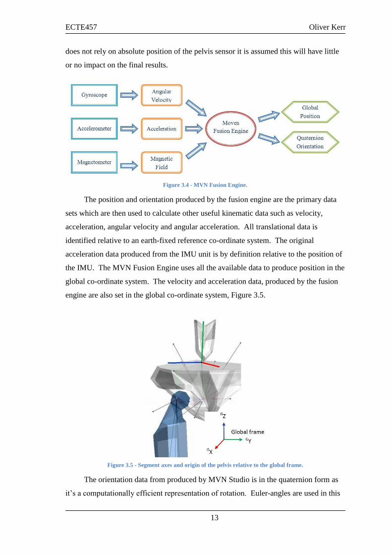
The MVN Fusion Engine, Figure 3.4, uses this data to produce the global position
and quaternion orientation of the body segment to which the sensor is attached. Xsens
has designed a filter called the Xsens Kalman Filter for 3 Degrees-of-Freedom. This
filter uses the data from the magnetometer to stabilise heading (yaw) and uses the
acceleration due to gravity to stabilise inclination (roll/pitch)[26]. Position drift is
suppressed by using knowledge of the human body and assumptions about the bodies
contact with the external environment. It should be noted that the position drift
suppression algorithm used with this system is incompatible with the goals of this
project as it uses data derived from the other sensors. However, because this thesis
ECTE457 Oliver Kerr
13
does not rely on absolute position of the pelvis sensor it is assumed this will have little
or no impact on the final results.
Figure 3.4 - MVN Fusion Engine.
The position and orientation produced by the fusion engine are the primary data
sets which are then used to calculate other useful kinematic data such as velocity,
acceleration, angular velocity and angular acceleration. All translational data is
identified relative to an earth-fixed reference co-ordinate system. The original
acceleration data produced from the IMU unit is by definition relative to the position of
the IMU. The MVN Fusion Engine uses all the available data to produce position in the
global co-ordinate system. The velocity and acceleration data, produced by the fusion
engine are also set in the global co-ordinate system, Figure 3.5.
Figure 3.5 - Segment axes and origin of the pelvis relative to the global frame.
The orientation data from produced by MVN Studio is in the quaternion form as
it‟s a computationally efficient representation of rotation. Euler-angles are used in this

ECTE457 Oliver Kerr
14
thesis to describe the orientation of the pelvis as they are the simplest. It is important,
therefore, to transform from the quaternion form, given by MVN Studio, to the Euler
form.
The unit quaternion can be described as a rotation about a unit vector n through
angle α, shown in Equation 3.1.
(3.1)
The general form for a quaternion is shown in Equation 3.2.
(3.2)
Equation 3.3 shows the unit quaternion.
(3.3)
Euler-angles provide a much more intuitive form of orientation. Each of the three
Euler-angles ϕ, θ and ψ correspond to roll, pitch and yaw/heading. They are of the
XYZ Earth fixed type, also known as the aerospace sequence. Equation 3.4, Equation
3.5 and Equation 3.6 define the symbols and show the range of the roll, pitch and yaw
respectively.
(3.4)
(3.5)
(3.6)
The Euler-angles are calculated from the unit quaternion using the relations of
Equation 3.7, Equation 3.8 and Equation 3.9.
(3.7)
(3.8)
(3.9)
Table 3.2 shows the typical performance of the orientation data from MVN
Studio.

ECTE457 Oliver Kerr
15
Table 3.2 - Orientation data performance [24].
Dynamic Range All angles in 3D Angular Resolution 0.05 deg Static Accuracy (Roll/Pitch) <0.5 deg Static Accuracy (Heading) <1 deg Dynamic Accuracy 2 deg RMS
The global reference frame is fixed during the calibration phase of each session:
Origin – the base of the right heel
X axis – points in the direction of magnetic north
Y axis – points in the direction of magnetic west
Z axis – points vertically upward
3.3 Matlab Extension
Matlab code to transform the data into SAX form is freely available from the
internet. Lin et al. [27] have produced a Matlab code which provides scripts that
convert time series data into symbols and compute the minimum distance between two
symbol strings. For reference purposes it is included on the accompanying CD.
Matlab code was also written specifically for this thesis and is detailed in the
Chapter 4.
3.4 Experimental Design Limitations of the MVN Package
One of the crucial features of the MVN Biomech system is that it is very versatile
in the environments that it can be used. The main restriction on the system is that the
wearer of the suit has to be within 150m of the wireless receivers, though not in line of
sight. Strong magnetic fields also influence the suit, however, it is completely immune
to interferences of less than 30 seconds and resistant to longer term disturbances.
The Biomech needs to be calibrated for every data collection session and for
every new user. For the MVN Studio to have an accurate model of the user body
dimensions must be supplied. This calibration increased the accuracy of the
calculations of body segments‟ translational position and orientation. The user is then
has to perform a number of calibration poses in order for MVN Studio to calculate the
original relative position of all sensors. These include the neutral pose, the T-Pose, the
squat and hand touch poses. This information is then used in the sensor fusion
algorithm.

ECTE457 Oliver Kerr
16
After calibration MVN Studio can record continuously or at intervals controlled
by the experimenter. Once the session has been completed MVN Studio can export the
data to files readable by other programs.
3.5 Inadvertent Effects of SAX and Sliding Windows
A key component of SAX is the normalisation of the time series upon which it is
performed [9]. By definition this removes the average value of the time series, thereby
acting as a high pass filter with a cut of value approaching zero. The value of the
individual symbols in a SAX representation of a time series is meaningless as they do
not represent an absolute value, rather they summarise the shape of the time series data
and have meaning only when compared against the other SAX symbols.
The simulation of streaming data using a sliding window compounds this effect.
The classification algorithm performs a SAX transformation on the entire buffer of
sliding window data on every iteration. This normalisation of only the data in the
sliding window buffer has the effect of increasing the cut off frequency of the SAX
HPF effect. The minimum frequency which the SAX summarised time series can
represent has a period the same size as the sliding window length. This means that the
inadvertent high pass filter has a cut-off frequency approximately equal to the inverse
of the length of the sliding window. The HPF effect is shown in Figure 3.6 where the
two sliding window positions produce the SAX words aaaddcddca and dbabaaccdd.
Since the two words use the same alphabet of four letters all information regarding the
actual magnitude of the original time series is lost.

ECTE457 Oliver Kerr
17
Figure 3.6 – The SAX representation of the sliding window buffer from the first position of the sliding window
is: aaaddcddca. The SAX representation of the sliding window buffer from the second position is dbabaaccdd.
The impact of this filtering effect on this thesis is the inability to use the primary
method to classify any static activities. Static activities, by definition, only contain a
zero frequency component meaning the SAX representation will be meaningless. A
secondary method of classification has been developed to compare the orientations of
the static activities so that the classification of these activities can still take place.
ECTE457 Oliver Kerr
18
4 Experimental Design
This chapter covers the design of the experiment to be carried out as well as some
of the Matlab programming that was peripheral to the main classification engine,
including some data processing algorithms as well as visualisation functions.
4.1 Activities
The activities classified in this thesis can be divided into three main categories:
static activities, dynamic activities and transitional activities. Static activities, such as
standing, sitting or lying down, are static in nature and are therefore hard to classify
using a SAX based classification system. SAX is much more useful in classifying
dynamic activities such as walking or running. The transitional activity is the
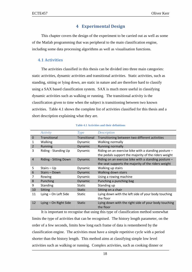
classification given to time when the subject is transitioning between two known
activities. Table 4.1 shows the complete list of activities classified for this thesis and a
short description explaining what they are.
Table 4.1 Activities and their definitions
Activity Type Description
0 Transitional Transitional Transitioning between two different activities 1 Walking Dynamic Walking normally 2 Running Dynamic Running normally 3 Riding - Standing Up Dynamic Riding on an exercise bike with a standing posture –
the pedals support the majority of the riders weight 4 Riding - Sitting Down Dynamic Riding on an exercise bike with a standing posture –
the seat supports the majority of the riders weight 5 Stairs – Up Dynamic Walking up stairs 6 Stairs – Down Dynamic Walking down stairs 7 Rowing Dynamic Using a rowing machine 8 Punching Dynamic Punching a punching bag 9 Standing Static Standing up 10 Sitting Static Sitting on a chair 11 Lying – On Left Side Static Lying down with the left side of your body touching
the floor 12 Lying – On Right Side Static Lying down with the right side of your body touching
the floor
It is important to recognise that using this type of classification method somewhat
limits the type of activities that can be recognised. The history length parameter, on the
order of a few seconds, limits how long each frame of data is remembered by the
classification engine. The activities must have a simple repetitive cycle with a period
shorter than the history length. This method aims at classifying simple low level
activities such as walking or running. Complex activities, such as cooking dinner or

ECTE457 Oliver Kerr
19
participating in a game of soccer, would require a higher level classification engine
which is able to group sequences of simple activities into higher level activities.
4.2 Matlab Algorithms
Matlab based programs form the basis of the entire classification engine. MVN
Studio collects the data streaming from the suit in real-time, however, it does not have
the functionality to stream the export data. Data sets are only exported in their entirety
once all the recording has finished. Matlab programs are used to import the MVNX
data into the Matlab workspace, preprocess the data, classify the data, filter the
classifications and compute the accuracy of the system. Matlab is also used to perform
peripheral functions such as data visualization using a number of different methods.
4.2.1 Localization of the Pelvis Axes
A major problem with the data in the MAT files is that all position, velocity and
acceleration vectors are relative to the global coordinates. That is, that the data for
walking forward in one direction is the negative of data walking forward in the opposite
direction. This is a major problem for identifying motion as it is irrelevant which
direction the motion is taking place. This only, however, applies to the heading as it is
important to have the pitch and roll relative to the global axis.
The pelvis velocity data shown in Figure 4.1 shows this problem. The data set
describes a person walking for 10 seconds in one direction turning around and walking
for 10 seconds in the opposite direction. It is clear from the figure that the
characteristics of the data are significantly influenced by the direction of the motion. It
should be noted that similar effects are seen in position and acceleration data.
The problem was solved using basic geometric mathematics. The Matlab script
„RotateAngle.m‟, refer to accompanying CD, was written to transform all the data in the
global x and y coordinates into local x and y coordinates.

ECTE457 Oliver Kerr
20
Figure 4.1 - Velocity vectors in global Axes.
Figure 4.2 - Geometric representation of Point P in both global and local Axes of the XY Plane.
Vector P, in Figure 4.2, can be described in terms of the global XY axis as well as
the local XY axis. By definition the angle formed by the global X axis, XG, and the
local X axis, XL, is equal to the angle of yaw, ψ. Similarly the angle formed by the
global Y axis, YG, and the local Y axis, YL, is equal to the angle of yaw, ψ. Equation
4.1 and 4.2 show the mathematical relationship between the global and local coordinate
systems. Refer to Appendix C for a full proof of this relation.
(4.1)
(4.2)
The position vector, however, was not fully rectified by this mathematical
solution. Performing this simple transformation on the position vector resulted in
dynamically changing the direction of the axis. As a result the position vector changes
from positive to negative from a change in yaw of 180 degrees. Figure 4.3 shows the
position vector from the same data set shown in Figure 4.2. The top graph shows the

ECTE457 Oliver Kerr
21
global position vector of the person walking forwards in the positive Y direction and
then turning and walking back to starting point. The middle graph shows the dynamic
position vector; as the person spins around the local axis spins as well. This means that
the (X, Y) description of the location of the spin changes even though the location in
the global axes remains static. The bottom graph shows the static local position vector
once the solution detailed below has been implemented. It shows that as the wearer of
suit only walks in the forward direction with respect to the local axis.
Figure 4.3 - Representation of the global position (top), incorrect (dynamic) local position (middle) and the
correct (static) local position (bottom).
The solution to this problem was found by differentiating the position vector then
transforming from the global axis to the local axis before integrating back to the
original form. This essentially calculates the velocity from the position vector,
transforms it to the local axes and then calculates the local position from the local
corrected velocity.
It should be noted that the position, velocity and acceleration vectors calculated
by the MVN Fusion Engine did not completely conform to the definitional relation
between position, velocity and acceleration. That is the vector produced by
differentiating the position vector in Matlab was not identical to the velocity vector
produced by the engine, similarly the vector produced by differentiating the velocity
vector was not identical to the acceleration vector produced by the engine. It is
assumed that the vectors from the MVN Fusion Engine are accurate and that all
calculations involving position, velocity and acceleration shall use these original
vectors.

ECTE457 Oliver Kerr
22
4.2.2 Accuracy Calculation
The accuracy of the classifier is an essential measure of success; it must be
calculated in a way that is robust. Since S H Lee et al. [16] fails to meet this criterion
for accuracy calculation and no other literature documents an algorithm a new
algorithm had to be developed. It was also essential to be able to calculate the accuracy
before and after the post-classification filter, so it is important to be able to easily
compute the accuracy ignoring transitional activities and taking into account transitional
activities.
The classification engine uses a history of the data to classify a single time
instant. This means that assuming the classifier has an accuracy of 100% the output
will still only be a subset of the correct classifications. The offset was found to relate to
the sliding window length in frames (N) and the history length (h) by Equation 4.1.
(4.1)
The accuracy algorithm used is best illustrated in pseudo code in Figure 4.4. The
basic algorithm counts each time the results match the correct classification and then
finds the proportion to the total valid results. It should be noted that valid results are
those which do not correspond to a transitional activity unless the post-classification
filter has been implemented.
Figure 4.4 - Accuracy calculation function pseudo code.
accuracy = ActivityClassificationAlgorithm (CR,CC,N,h,preFilter)
// CC = Correct Classification
// ER = Classification Engine Results
// N = Sliding Window Length
// h = History Length
// preFilter = Boolean value controlling whether the transitional activities are
ignored
offset = N+historyLength-1;
sum = 0;
count = 0;
for i = 1 to length of CE
if preFilter
if CC(offset-1+i) != 0
sum = sum + (CC(offset-1+i) == CE(i));
count = count + 1;
end
else
sum = sum + (CC(offset-1+i) == CE(i));
count = count + 1;
end
end
accuracy = sum/count;
ECTE457 Oliver Kerr
23
4.3 Matlab Visualisation
Apart from regular graphs and charts it is important to visualise data in novel but
informative ways. To this end two scripts have been developed, one to animate the
orientation data of the pelvis and another to draw Time Series Bitmaps from SAX
strings.
4.3.1 Animation of the Pelvis Orientation using Matlab
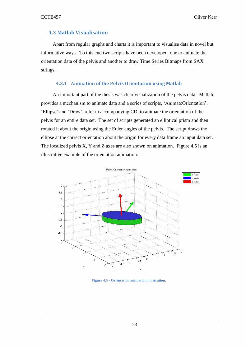
An important part of the thesis was clear visualization of the pelvis data. Matlab
provides a mechanism to animate data and a series of scripts, „AnimateOrientation‟,
„Ellipse‟ and „Draw‟, refer to accompanying CD, to animate the orientation of the
pelvis for an entire data set. The set of scripts generated an elliptical prism and then
rotated it about the origin using the Euler-angles of the pelvis. The script draws the
ellipse at the correct orientation about the origin for every data frame an input data set.
The localized pelvis X, Y and Z axes are also shown on animation. Figure 4.5 is an
illustrative example of the orientation animation.
Figure 4.5 - Orientation animation illustration.

ECTE457 Oliver Kerr
24
4.3.2 SAX Bitmap
The Matlab script „bitmap‟, refer to accompanying CD, transforms a SAX string
into a Time Series Bitmap. It can handle any string length but only has a sliding
window length of two.

ECTE457 Oliver Kerr
25
5 Classification Engine Design
The classification engine performs a number of distinct operations to transform
the raw incoming data into the end classified activities. The first task the engine
performs is the extraction of relevant data from the MVNX file and transforms it into a
Matlab friendly MAT format. A number of pre-processing operations take place at this
stage. The engine then further extracts examples of activities with which activity
templates are produced. These templates are then used by the core activity classifier to
classify full data sets. The raw results are then filtered to produce the requisite output.
The different stages of the classification engine are shown as the orange blocks of
Figure 5.1.
.
Figure 5.1 - Flow Diagram of classification engine and development functions.

ECTE457 Oliver Kerr
26
The blue blocks of Figure 5.1 show some of the various functions and outputs
used in the development of the engine. The accuracy computation function was a
simple comparison between the results generated by the engine and a perfect set of
results generated by human judgement. The parameter generation function was a
simple function which generated a range of different parameters, these were then tested
and the impact on the final outcome was determined. There were also a number of
functions which visualised various variables and data which were essential in analysing
the engine.
It is also important to note the correct classification of activities with which the
templates are generated and the accuracy of the results determined was produced by
human judgement of the data set. MVN Studio provides a lifelike animation of the data
from which human classifications can be made. In a future implementation a
calibration step can be substituted in order to produce the templates removing the need
for any human interaction.
5.1 Data Extraction
The data extraction process extracts the verbose MVNX data and transforms it
into a more useful form. Unwanted data that does not relate directly to the pelvis is
discarded. Pre-processing of the data also takes place. The Euler Angles are calculated
from the quaternion vectors. The data translational data is also transformed from the
global co-ordinate system to a local-coordinate system based upon the pelvis using the
orientation data as detailed in section 4.2.1. The data is then saved in a new MAT file
ready for future use.
5.2 Template Creation
An activity template is created for each activity which consists of five Time
Series Bitmaps, one for each acceleration dimension and one for two of the orientation
dimensions. It is important to note that the heading is not included in the templates
because it is heavily influenced by the direction in which the person is facing whilst
wearing the IMU. The templates are created from five second long data sequences of
each activity. These data sequences were manually extracted from each of the data sets
to represent all of the dynamic activities from each test subject.

ECTE457 Oliver Kerr
27
One of the experiments performed on the data compared the accuracy of the
classifier with different sliding window lengths (n) and frame to symbol rates (R). The
templates were influenced by these n and R values and so it was important to generate
these on every new set of values.
Another experiment was carried out to compare the different accuracy rates
between personal and default template generation. Personal templates, drawn from a
test subjects own data were then used to classify that persons data. Default templates
were drawn from general examples of each activity. It was important to differentiate
between personal and default templates. It should be noted that although the some of
the templates were computed from sequences within the data sets that were being
classified, each subject performed an activity for approximately 30 seconds. With only
five second sequences used for template generation, the overwhelming majority of data
is not used to generate the templates.
5.3 Classifier
The classifier treats the block of pelvis input data as a streaming data source by
processing the data using a sliding window. On each iteration of the algorithm the next
data frame is appended onto a history of recent data frames; the length of the history is
kept constant by concurrently removing the oldest data frame. This effectively
represents streaming data which is incremented by one data frame per iteration of the
program.
It is important to note that the algorithm used for this classifier was an adaption
and extension of a short pseudo code developed by Kasetty et al.[14].

ECTE457 Oliver Kerr
28
Figure 5.2 – Flow diagram showing the behaviour of the classification engine.
The history of recent data is then classified by the function using either the static
or dynamic classification algorithm. This is dependent on the average of each of the
three acceleration dimension‟s standard deviation. Before the actual classification of
the dynamic activities can take place two extra transformations are performed on the
data, each dimension of the time series is summarised using SAX and then used to
create a Time Series Bitmap. Figure 5.2 shows the flow of the classifier. See Figure
5.3 for examples of the TSBs produced from the sliding window of data and the
template TSBs. It is visually clear from the figure that the example TSBs most closely
resemble the walking activity template.

ECTE457 Oliver Kerr
29
Figure 5.3 Example of the TSBs produced by the sliding window in the classification program and the master
template TSBs that they are compared too. Table 5.1 shows the Euclidean Distance measurements. It should
be noted that in this example only the acceleration TSBs are shown, the classification program also compares
the X and Y orientation TSBs.
The static and dynamic classification algorithms use very similar methods to
classify the data. The static algorithm finds the Euclidean Distances between the
orientation of the current data set and the orientations of each of the activity templates.
The dynamic algorithm finds the Euclidean Distances between the TSBs of the sliding
window of data and the template TSBs. The activity templates are then ranked on the
average Euclidean Distance to the current sliding window of data. The resultant
classified activity is chosen to be the closest match. Table 4.1 shows the calculated
Euclidean Distance measurements between the sets of TSBs shown in Figure 5.3. In
this case the classification result is walking because it is much closer to the walking
template than the running template. It should be noted, however, that the classification
function takes into account the roll and pitch as well as the accelerations.

ECTE457 Oliver Kerr
30
Table 5.1 – Euclidean distance measurements between the sliding window TSBs and template TSBs from
Figure 5.3
Activity X - Axis Y - Axis Z - Axis Average
Walking 0.6137 0.5152 0.0587 0.3959
Running 0.7600 1.7085 1.7333 1.4006
5.4 Post Classification Filter
The post classification filter removes from the classification stream any activities
that are not performed for longer than seven seconds. Experimentally it was found that
the activity classification was not consistent when there was a transition from one
activity to another, this meant that in a short space of time multiple different activities
were deemed to take place. This simple filter replaced any activity that had a period
less than the threshold with the „transitional‟ activity.
Figure 5.4 illustrates an example of unfiltered output highlighting the correctly
and incorrectly classified activities as well as the transitional activities which are
deemed to be neither correct nor incorrect. Whilst the subject is performing an activity
transition, it was observed that the results of the activity classification were short bursts
of a random activity.
Figure 5.4 - Results of activity classification sans filtering.
Figure 5.5 shows results once they have been filtered. It is clear that the
transitions between activities are classified with a fair success rate. It is important to
note that the correct classifications that the results are compared against were human
generated from observing the animation of the data. The exact moment of one activity

ECTE457 Oliver Kerr
31
ending and another beginning is at best only an estimation of a human. This is
especially true for the transitional activity.
Figure 5.5 – Filtered output of classification engine.
ECTE457 Oliver Kerr
32
6 Experimental Work and Results
In this chapter the work undertaken in collecting and managing the data is
detailed as well as the experiments and results. A large data library, collected from
previous and current theses, was made available; a specific data collection experiment
was also carried out for the purposes of this thesis in which three subjects performed
various activities. Experiments were then carried out on these results which compared
the impact of using individual or default templates, various sliding window buffer
lengths, SAX subword sizes and frame to symbol rates. A validation experiment was
also undertaken using motion capture data obtained from an online database provided
by Carnegie Mellon University.
6.1 Data Collection
6.1.1 Previously Collected Data
An extensive array of data has been collected prior to this thesis which has been
used for the purposes of this thesis. Over 10 gigabytes of data with 30 minutes of
motion capture covering a wide range of motions and behaviors. They include:
Walking – variations on walking are also included such as walking backwards,
walking with gait problems and walking with weights
Running – jogging included
Balancing – balancing on one foot and balancing on a ball
Stepping – climbing up and down steps with and without weights
Waitering – picking objects up using a tray
Sporting skills – including golf swings, tennis swings, and hockey skills
Static Manipulation of Objects – sitting down and manipulating objects on a
desk
This data was used in the development of the many of the visualization functions,
and much of the classification engine. This data was, however, limited in that the
majority of sequences were short, on the order of five to ten seconds in length and
included only one activity. As a result this data was not used to test and improve the
final classification engine.

ECTE457 Oliver Kerr
33
6.1.2 Activity Classification Data
On the 17th
of September an experiment was carried out with three different test
subjects performing the full range of classifiable activities. Each activity was
performed only once for a period of approximately 30 seconds. The order of the
activities was randomized for each test subject. Figure 6.1 shows some of the activities
undertaken during the data collection session.
Figure 6.1 – Photos from the data collection session. Clockwise from top left photo: Walking up the stairs,
rowing, cycling sitting down, punching bag, lying down on the left side, walking.
6.1.3 Correct Activity Classification
In order to analyse the accuracy of results they must be compared to a correct
classification of the activities. This correct classification of the activities was
performed using full body animation of MVN Studio. The data was divided up into 100
frame sequences which were then classified into the thirteen different activities. The

ECTE457 Oliver Kerr
34
results were then saved into a MAT file, ready for use in the analysis of results. Figure
6.2 shows the correctly classified data of each of the three subjects.
Figure 6.2 - Correct classifications of each subject.
It is important to note that the walking up stairs activity is intermingled with the
walking down stairs activity. This is a result of only a very short flight of stairs, only
eight steps in length, being available. The activities were performed together in one 60
second long sequence of walking up and down the stairs. As detailed in section 6.2.3
this caused a problem for the classification engine because each particular sequence of
moving up and down stairs was shorter than the threshold of the post classification
filter. The solution was to concatenate together the walking up stairs and walking down
stairs into one long sequence of each activity. The modified correct classifications are
shown in Figure 6.3. It should be noted that the data for each subject was modified in
accordance with modification of the correctly classified vectors; that is all the walking
up stairs data was grouped and all the walking down stairs data was grouped.
Figure 6.3 - Modified correct classifications of each subject.
ECTE457 Oliver Kerr
35
6.2 Optimisation of the Classification Engine
The classification engine had a number of parameters which directly affected its
performance which were optimised through experimentation. These included the
history buffer length, the post-classification filter threshold, length of the sliding
window, frame to symbol rate, and the symbol frequency rate. Equation 5.1 shows the
relationship between the sliding window length in frames (N), sliding window length in
symbols (n), the frame frequency rate (fF = 120 Hz), the symbol frequency rate (fS) and
the frame to symbol rate (R).
(5.1)
6.2.1 Impact of the Sliding Window Length and Frame to Symbol Rate
The sliding window length and the symbol to frame rate have a significant impact
on the SAX representation of the data. It was observed experimentally that these
parameters also had a significant impact on the accuracy of the final outcome. It is
important to note that these two parameters are tested together as the impact of each is
affected by the other; it is therefore invalid to test each independently.
The sliding window was tested in the range from four to 40 symbols and the
frame per symbol rate was tested in the rage of two to 28. For this experiment the
history length was set at 300 frames, the filter threshold, when used, was set at seven.
These parameters were perhaps the most influential of all to be optimised; the impact
was tested on both default and individually generated templates.
Figure 6.5 and Figure 6.6 show the effects of the sliding window length and the
frame to symbol rate on default and individually generated templates respectively. It is
exceedingly clear that the impact is greatly reduced when it is tested on classifications
made from individually generated templates. The average accuracy from default
templates ranges from 40% to 85%, peaking with a sliding window length of
approximately 10 to 12 symbols and a frame to symbol rate of 20. The average
accuracy from the individually generated templates is much more resilient to these
parameters; it ranges from 80% to 90%.

ECTE457 Oliver Kerr
36
Figure 6.4 – Effect of the sliding window length and the frame to symbol rate on the accuracy of filtered
classifications from default templates.
Figure 6.5 – Effect of the sliding window length and the frame to symbol rate on the accuracy of filtered
classifications from individual templates.

ECTE457 Oliver Kerr
37
The heavy impact of these parameters on the default template classification
method results from the differences in the data produced by each subject performing the
same activity. The values of these parameters which correspond to the highest accuracy
best retain the data features common to all subjects while minimising the differences
between them. This also explains why the impact is so small on the classifications from
individually generated templates; all the data features, irrespective of their commonality
between subjects, correspond to a certain activity. The best values for n and R were
found to be 12 and 20 respectively.
6.2.2 Impact of the History Buffer Length
The history length controls the number of frames that the classification engine
stores in memory in order to classify the data. A longer history length means the
impact of each particular data frame is reduced because it is a smaller part of the data.
This means that the engine is more robust to small inconsistencies in the data. A
shorter history length means less data is used to make each classification, meaning an
activity performed for a shorter period of time can be classified.
Figure 6.6 - Effect of history length on accuracy.
Figure 6.6 shows effect of the history length on the filtered classifications
generated from default templates. It is clear from the graph at there is a substantial
amount on „noise‟ in this effect as the accuracy of each subject both increases and
decreases, seemingly at random, across the range of history lengths. Within this range,
however, the effect is limited to less than a 10% difference for all of the subjects. The

ECTE457 Oliver Kerr
38
average shows a peak accuracy at a 250 to 300 frame history length. From this
experiment the history length of all other experiments was chosen to be 300 frames.
The reason that the accuracy increases with history length, up to a point, is that
the impact of small errors and inconsistencies in the data is lessened. The history length
also effects how many frames of activity are needed to classify it as that activity and so
it takes longer for an activity to be classified. This effect becomes dominant and the
accuracy decreases once the length reaches 300.
It is also important to note that the history length also has a significant impact on
the amount of memory used and the speed of the classification engine. It is therefore
better to have a history length as small as possible to make sure the engine is efficient in
terms of speed and resources usage.
6.2.3 Impact of the Post-Classification Filter
The post-classification filter replaces the activities which are classified to have a
duration of less than the threshold with the transition activity. The threshold value was
tested in the range of 1 to 20 and its effect on the accuracy calculated. Figure 6.7 shows
the effect of the threshold on the accuracy of the classifications for each of the subjects.
There was a clear common peak at a threshold of seven seconds
Figure 6.7 – Impact of the threshold on the accuracy of classification when individually generated templates
were used.
It is important to note that of the original data sequences the period of sequence of
walking up and walking down stairs did not last five seconds. Any correct

ECTE457 Oliver Kerr
39
classification of walking up and down stairs would therefore be filtered out because the
threshold of seven seconds is not reached. This was anticipated and so all of the data
sequences pertaining to each of the walking up and down stairs activities has been
concatenated together to form two long sequences of walking up and down stairs. The
accuracy both the stairs classification, whilst still in individual sequences, ranged from
20% to 70% when using default templates, and 85% to 100% when using individual
templates. All other experiments are performed on the concatenated stairs data to
ensure comparability between filtered and unfiltered accuracy.
6.2.4 Final Classification Engine
All experiments have been designed and undertaken with the view to optimise the
parameters of the classification engine; the optimised engine has been tested and
analysed. Table 6.1 shows the overall accuracy results of the classification engine. It is
obvious that the individual templates provide a much more robust method of
classification with all results having an accuracy of approximately 95%. The default
template generation method provides results of a much wider range, on the order of
25%. The optimal method of classification, for a product using this engine, would be
individual templates, produced by a simple calibration process. Default templates,
although, clearly not as accurate would provide the capability to skip a calibration stage
for simple, quick or en masse implementation.
Table 6.1 – Accuracy of classification engine for each subject for both default and individual templates
Test Subject Default Template Individual
Template
1 71% 96%
2 94% 96%
3 84% 94%
Average 83% 95%
Table 6.2 is the confusion matrix generated from the results of all three test
subjects data using the default template generation method. It is clear that the riding an
exercise bike whilst sitting down was difficult to classify by the engine, misclassifying
it as punching. A substantial amount of walking was also classified as punching,
though it is not clear why this is so. The translational activity was misclassified more
than 50% of the time, this is because the exact point in time which a person starts
transitioning from an activity or stops transitioning to an activity is subjectively judged
by a person.

ECTE457 Oliver Kerr
40
Table 6.2 - Confusion matrix from all three test subjects using default templates. Note all values are a
percentage of the total value (%).
Correct
Activities
Predicted
Activities Tra
nsi
tio
na
l
Wa
lkin
g
Ru
nn
ing
Rid
ing
–
Sta
nd
ing
Up
Rid
ing
–
Sit
tin
g D
ow
n
Sta
irs
- U
p
Sta
irs
- D
ow
n
Ro
win
g
Pu
nch
ing
Sta
nd
ing
Sit
tin
g
Ly
ing
Do
wn
–
On
Lef
t
Ly
ing
Do
wn
–
On
Rig
ht
Transition 42 6 2 2 3 27 6 0 1 6 8 4 0
Walking 3 67 0 0 0 0 0 0 0 0 0 0 0
Running 3 0 98 0 0 10 29 0 0 0 0 0 0
Riding –
Standing Up 1 0 0 95 0 0 0 0 0 0 0 0 0
Riding –
Sitting Down 0 0 0 0 31 0 0 0 0 0 0 0 0
Stairs – Up 1 0 0 0 0 60 0 0 0 0 0 0 0
Stairs – Down 2 0 0 0 0 0 63 0 0 0 0 0 0
Rowing 27 0 0 0 1 3 2 100 0 4 5 4 7
Punching 9 28 0 2 65 0 0 0 99 0 1 0 0
Standing 2 0 0 0 0 0 0 0 0 91 1 0 0
Sitting 6 0 0 0 0 0 0 0 0 0 85 0 0
Lying Down –
On Left 2 0 0 0 0 0 0 0 0 0 0 91 0
Lying Down –
On Right 2 0 0 0 0 0 0 0 0 0 0 0 93
Table 6.3 shows the confusion matrix generated from all three test subjects using
the individual templates method. The matrix shows that the classifier is perfect at
differentiating between defined activities, there is not a single instance, for all three test
subjects of misclassifying one activity as another. Where the classifier falls down,
however, is when filtering the classified data and adding in the transitional data; only
66% of the transitional activity is correctly classified. This is not surprising however,
as the judgement of the exact moment when an activity starts and ends and the
transition begins and ends is quite subjective.
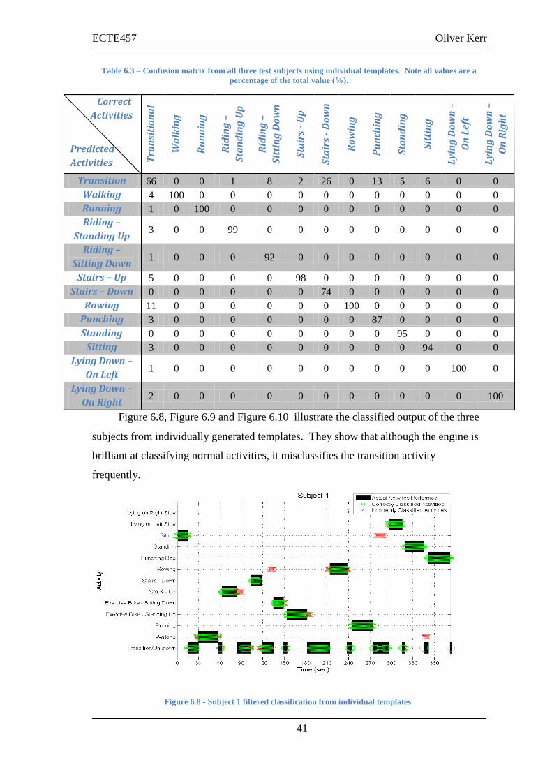
ECTE457 Oliver Kerr
41
Table 6.3 – Confusion matrix from all three test subjects using individual templates. Note all values are a
percentage of the total value (%).
Correct
Activities
Predicted
Activities Tra
nsi
tio
na
l
Wa
lkin
g
Ru
nn
ing
Rid
ing
–
Sta
nd
ing
Up
Rid
ing
–
Sit
tin
g D
ow
n
Sta
irs
- U
p
Sta
irs
- D
ow
n
Ro
win
g
Pu
nch
ing
Sta
nd
ing
Sit
tin
g
Ly
ing
Do
wn
–
On
Lef
t
Ly
ing
Do
wn
–
On
Rig
ht
Transition 66 0 0 1 8 2 26 0 13 5 6 0 0
Walking 4 100 0 0 0 0 0 0 0 0 0 0 0
Running 1 0 100 0 0 0 0 0 0 0 0 0 0
Riding –
Standing Up 3 0 0 99 0 0 0 0 0 0 0 0 0
Riding –
Sitting Down 1 0 0 0 92 0 0 0 0 0 0 0 0
Stairs – Up 5 0 0 0 0 98 0 0 0 0 0 0 0
Stairs – Down 0 0 0 0 0 0 74 0 0 0 0 0 0
Rowing 11 0 0 0 0 0 0 100 0 0 0 0 0
Punching 3 0 0 0 0 0 0 0 87 0 0 0 0
Standing 0 0 0 0 0 0 0 0 0 95 0 0 0
Sitting 3 0 0 0 0 0 0 0 0 0 94 0 0
Lying Down –
On Left 1 0 0 0 0 0 0 0 0 0 0 100 0
Lying Down –
On Right 2 0 0 0 0 0 0 0 0 0 0 0 100
Figure 6.8, Figure 6.9 and Figure 6.10 illustrate the classified output of the three
subjects from individually generated templates. They show that although the engine is
brilliant at classifying normal activities, it misclassifies the transition activity
frequently.
Figure 6.8 - Subject 1 filtered classification from individual templates.

ECTE457 Oliver Kerr
42
Figure 6.9 – Subject 2 filtered classification from individual templates.
Figure 6.10 – Subject 3 filtered classification from individual templates.
6.3 Validation of Engine
It is very important that the engine be validated using a data set that was not used
in its development. A suitable data set was found on an online database of freely
available motion capture data provided by Carnegie Mellon University[28]. The data
set is composed of 15 different types of walking listed in Table 6.4. It should be noted
that since all the activities are comprised solely of sub-types the essentially the same
activity that the difficulty of classification is exceedingly high.
The engine was slightly modified to cope with this new data set as there were no
static activities to classify. It should also be noted that the templates were generated by
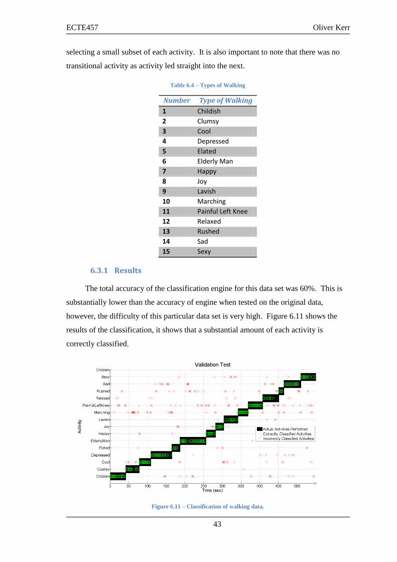
ECTE457 Oliver Kerr
43
selecting a small subset of each activity. It is also important to note that there was no
transitional activity as activity led straight into the next.
Table 6.4 – Types of Walking
Number Type of Walking
1 Childish
2 Clumsy
3 Cool
4 Depressed
5 Elated
6 Elderly Man
7 Happy
8 Joy
9 Lavish
10 Marching
11 Painful Left Knee
12 Relaxed
13 Rushed
14 Sad
15 Sexy
6.3.1 Results
The total accuracy of the classification engine for this data set was 60%. This is
substantially lower than the accuracy of engine when tested on the original data,
however, the difficulty of this particular data set is very high. Figure 6.11 shows the
results of the classification, it shows that a substantial amount of each activity is
correctly classified.
Figure 6.11 – Classification of walking data.

ECTE457 Oliver Kerr
44
7 Conclusions
In this chapter the outcomes of this project are discussed with particular focus on
how they related to the goals set out in the project scope. A section on future work is
also included.
7.1 Comments
7.1.1 Matlab and a Future Implementation
Matlab was chosen as the basis for engine because it is an extremely useful data
analysis tool. It contains a multitude of useful functions for visualising and
manipulating the data. It combines the functionality of Java with the accessibility of a
deceptively simple interface. These features make it very useful as a development tool
and this is why it was used to develop the engine.
The classification engine, although programmed in Matlab, does not use any
Matlab specific tools and can easily be implemented in other languages. As Matlab
uses a Java, which runs in a virtual machine on the computer, the functions run in
Matlab are not nearly as computationally efficient as similar programs compiled from
other languages [29]. It should also be noted that the peripheral functions extensively
used in Matlab whilst the engine was in development, not easily available in other
languages, will not be needed in the final product.
A future implementation of this classification tool should therefore be coded in
computationally efficient language ensuring the real-time functionality of the engine is
preserved.
7.2 Outcomes
The success of this classification engine is comparable other attempts at
classification of motion capture data as shown in Table 7.1. The engine performs as
well as the Kasetty et al.[14] which is the only other team to attempt to validate their
engine by classifying other data. It is important to note that this engine had the added
difficulty of performing the classifications in pseudo real-time and on pseudo streaming
data.

ECTE457 Oliver Kerr
45
Table 7.1 – Comparison of classification accuracy between different methods. *Not motion capture data.
**Average.
Team Accuracy on Own Data Validation Accuracy
Classification Engine 83/95% 60% *Kasetty et al.[14] 95% **66% Parkka et al.[30] 82/86/82% Najafi et al.[17] **90% Saponas et al. [18] 97/99%
7.2.1 Every Day Activities
The twelve activities classified, excluding the transitional activity, do not fully
encompass the activities normally undertaken on a daily basis. The focus has been on
simple activities that provide stable data, that is a few second sliding window of a
particular activity will produce a constant Time Series Bitmap. As stated in 4.1 higher
level activities that change from moment to moment will not be able to be processed by
this algorithm; a higher level algorithm which draws together simple sub-activity
classifications into an overarching activity would be needed.
The stated aim, therefore, to produce a data classification tool which would
classify the streaming data from an IMU into the daily activities has not been met as the
list of activities which can be classified does not encompass the entire list of plausible
daily activities. A tool has been developed, however, which does classify simple
activities and differentiate between activities and activity transitions. It can be used as a
cornerstone in a higher level classifier which will be able to classify a realistic list of
everyday activities.
7.2.2 Ease of Adding New Activities
Previous motion classification attempts have used methods which require
training. This means that for every new activity that is added to the list of classification
activities the classifier must be retrained. It would be exceptionally difficult or
impossible to give end users of a product the ability to retrain the classifier to allow new
activities to be classified.
A major advantage of this method is ease of adding new activities to the list of
classifiable activities. The engine needs only a short sequence of the new activity from
which to produce a template. A future product using this engine could easily
incorporate a feature that allows the user to add a new activity simply by selecting an

ECTE457 Oliver Kerr
46
option on interactive software and then performing the new activity for a short period of
time. To the extent of the literature reviewed for this thesis, no other motion
classification method allows this feature.
7.3 Future Work
7.3.1 Development of Current Engine
Although quite successful at classifying the activities within this thesis, a
substantial amount of work needs to be done at finding new activities which can be
classified as well as optimising the algorithms and processes.
7.3.2 Development of Higher Level Classifier
An important future direction for this work is to develop a classifier that is able to
use the low level classifications of sub-activities to classify high level activities. An
example of this would be using the sub-activity classifications of chopping, stirring,
pouring and mixing to classify cooking. Further improvements could be made by using
a memory of previously performed activities, for example showing would most likely
be followed by getting dressed. Other ideas such as incorporating the time of day, from
a timer, and the location, from a GPS, could be used, for example playing tennis could
only occur on a tennis court.
7.3.3 Developing of Complete Package to Use
This thesis was completed with the use of the MVN Biomech and the MVN
Studio software package. This somewhat limited the practical scope of this thesis in
terms of the amount of sensors used and the ability to process streaming data. It is
important for future development of a complete hardware and software package; the
realisation of the original goal of performing real-time classification of everyday
activities using a single IMU.

ECTE457 Oliver Kerr
47
8 References
[1] Greg W Scragg, Problem Solving with Computers, Illustrated ed. Massachusetts,
USA: Jones & Bartlett Learning, 1997.
[2] Hermann Kopetz, Real-Time Systems: Design Principles for Distributed Embedded
Applications. New York, USA: Springer, 1998.
[3] Xsens Technologies B.V. (2009) Xsens MVN BIOMECH User Manual.
[4] George Almasi and David Padua, "MaJIC: Compiling MATLAB for Speed and
Responsiveness," SIGPLAN Not., vol. 37, no. 5, pp. 294-303, May 2002.
[5] Adam Drewnowski and William J Evans, "Nutrition, Physical Activity, and
Quality of Life in Older Adults: Summary," Journals of Gerontology, vol.
56, no. 2, pp. 89-94, October 2001.
[6] Nathan Miller, Chadwick Jenkins, Marcelo Kallman, and Maja J Mataric, "Motion
Capture from Inertial Sensing for Untethered Humanoid Teleoperation," in
International Conference of Humanoid Robotics, Los Angeles, 2004, pp.
547-565.
[7] Daniel Vlasic et al., "Practical Motion Capture in Everyday Surroundings," ACM
Transactions on Graphics, vol. 26, no. 3, July 2007.
[8] Eamonn Keogh. Welcome to SAX (Symbolic Aggregation approXimation).
[Online]. http://www.cs.ucr.edu/~eamonn/SAX.htm
[9] Jessica Lin, Eamonn Keogh, Stefano Lonardi, and Bill Chiu, "A Symbolic
Representation of Time Series, with Implications for Streaming Algorithms,"
in 8th ACM SIGMOD workshop on research issues in data mining and
knowledge discovery, San Diego California, 2003, pp. 2-11.
[10] Eamonn Keogh, Kaushik Chakrabarti, Michael Pazzani, and Sharad Mehrotra,
"Dimensionality Reduction for Fast Similartiy Search in Large Time Series
databases," Knowledge and Information Systems, vol. 3, no. 3, pp. 254-286,
August 2001.
[11] Eamonn Keogh, Jessica Lin, and Stefano Lonardi, "Experiencing SAX: A Novel
Approach to Time Series," Data Mining and Knowledge Discovery, vol. 15,
no. 2, pp. 107-144, October 2007.
[12] Christos Faloutsos, M Ranganathan, and Yannis Manolopoulos, "Fast Subsequence
ECTE457 Oliver Kerr
48
Matching in Time-Series Databases," in ACM SIGMOD International
Conference on Management of Data, Minneapolis, 1994, pp. 419-429.
[13] Natin Kumar, Nishanth Lolla, and Eamonn Keogh, "Time-Series Bitmaps: a
Practical visualisation Tool for Working with Large Time Series databases,"
in SIAM 2005 Data Mining Conference, Los Angeles, 2005, pp. 531-535.
[14] Shashwati Kasetty, Candice Stafford, Gregory P Walker, Xiaoyue Wang, and
Eamonn Keogh, "Real-Time Classification of Streaming Sensor Data," in
ICTAI 20th IEEE Conference on Tools with Artificial Intelligence, Dayton,
2008, pp. 149-156.
[15] J Bussman et al., "Measuring Daily Behaior Using Ambulatory Accelerometry:
The Activity Monitor," Behavior Research Methods, Instruments, &
Computers, vol. 33, no. 3, pp. 349-356, August 2001.
[16] S H Lee, H D Park, S Y Hong, K J Lee, and Y H Kim, "A Study on the Activity
Classification Using a Triaxial Accelerometer," in 25th Annual International
Conference of the IEEE EMBS, Cancun, 2003, pp. 2941-2943.
[17] Bijan Najafi et al., "Ambulatory System for Human Motion Analysis Using a
Kinematic Sensor: Montioring of Daily Physical Acticity in the Elderly,"
IEEE Transactions on Biomedical Engineering, vol. 50, no. 6, pp. 711-723,
June 2003.
[18] T Saponas, J Lester, J Froehlich, J Fogarty, and J Landay, "iLearn on the iPhone:
Real-Time Human Activity Classification on Commodity Mobile Phones,"
Univesity of Washington, Seattle, Technical Report 2008.
[19] Chao Sun, "Human Behavioural Skills Modelling and Recognition," University of
Wollongong, Wollongong, Masters Thesis 2007.
[20] Usama M Fayyad, Georges G Grinstein, and Andreas Wierse, Information
Visualisation in Data Mining and Knowledge Discovery, Diane D Cerra, Ed.
San Diego, USA: Academic Press, 2002.
[21] David Hand, Heikki Mannila, and Padhraic Smyth, Principles of Data Mining.
Massachusetts, USA: MIT Press, 2001.
[22] F Morchen, "Time Series Knowledge Mining," Philipps-University, Marburg, PhD
Thesis 2006.

ECTE457 Oliver Kerr
49
[23] Eamonn Keogh et al., "Intelligen Icons: Integrating Lite-Weight Data Mining and
Visualiztion into GUI Operating Systems," ICDM, pp. 912-916, 2006.
[24] Xsens Technologies B.V. (2009) Xsens. [Online]. http://www.xsens.com
[25] Xsens Technologies B.V. (2009) Xsens. [Online]. http://www.xsens.com
[26] Xsens Technologies B.V. (2008, October) LPK. [Online]. http://lpk.com
[27] J Lin, E Keogh, S Lonardi, and B Chiu. (2006) SAX. [Online].
http://cs.gmu.edu/~jessica/sax.htm
[28] Carnegie Mellon University. (2010, Octoboer) CMU Graphics Lab Motion Capture
Database. [Online]. http://mocap.cs.cmu.edu/
[29] Stephen J Chapman, MATLAB Programming for Engineers, 4th ed. Belmont,
USA: Thomson Wadsworth, 2008.
[30] Juha Parkka et al., "Activity Classification Using Realistic Data from Wearable
Sensors," IEEE Transaction on Information Technology in Biomedicine, vol.
10, no. 1, pp. 119-128, January 2006.

ECTE457 Oliver Kerr
50
A Appendix A – Original Project Plan
Project Proposal:
An important indicating factor of the quality of life of persons with limited
mobility is the identification of physical activity. Health Related Quality of Life
(HRQL), as measured, in part, by the Activities of Daily Living Score is a reflection of
the “personal sense of physical and mental health and the capacity to react to diverse
factors in the environment.”1
In 1960 the proportion of people over 65 to those of working age was 15%, by
2030 the proportion will increase to 35% in all OECD countries2. In Australia the cost
of aged care will increase by 0.39 percentage points of GDP from 2006 to 20313.
It is important therefore to be looking at finding cheaper alternatives to any tasks
currently undertaken in aged care. The use of a wearable IMU to measure the daily
activities of limited mobility people may be cheaper or more accurate than the current
solutions.
The project goal would be to produce a data analysis tool which would readily
classify the data from an IMU into the daily activities of the wearer.
The device being used to capture kinetic motion would be MVN Biomech made
by Xsens. The device senses kinematic motion using a tri-axis accelerometer, a tri-axis
gyroscope and a tri-axis magnetometer. It has wireless communication interface with a
range of up to 150 metres of open space and 50 metres of “office space”.
A crucial step in the project is to collect data by wearing the IMU device and
perform certain tasks and activities. It is important to then find correlations between
certain activities and the corresponding characteristics and patterns in the data.
The crux of this thesis project is accurately classifying daily activities from data
produced by the IMU. There are a number of techniques already used to perform this
1 Adam Drewnowski and William J. Evans, Nutrition, Physical Activity, and Quality of Life in
Older Adults: Summary, Journals of Gerontology: Oct 2001: 56A, Research Library, pg 89, 2 OECD, 1998. Maintaining Prosperity in an Ageing Society. Organisation for Economic Co-
operation and Development, Paris. 3 Madge, A, 2000, Long-Term Aged Care: Expenditure Trends and Projections, Productivity
Commission Staff Research Paper, Canberra, October.

ECTE457 Oliver Kerr
51
task but it is important to try novel solutions. Symbolic Aggregate approXimation
(SAX) is a powerful tool that has not yet been applied to this problem.
The first task involved in this project will be to perform a literature review which
would identify current research and future applications of the project. Data would also
need to be collected, meaning the device would need to be worn and the user perform a
certain range of activities. The data would then be divided up into sets corresponding to
the activities performed so that the important characteristics can be identified. SAX
would then be used to recognise the characteristics in the data and then translate that
back to the activities performed by the user. Testing would need to be performed to
ensure the daily activity recognition is accurate.
Thesis Objectives:
Data collection analysis: Use various filters, data transformation and data
analysis tools to transform the data into a usable form.
Classification of Daily Activities: Once the data has been properly
analysed it can then be „mined‟ for the defining characteristics of each daily
activity. It is the objective of the project to classify as many normal daily
activities as possible, on the order of 10 to 20 activities.
Create an Automatic Analysis Software Tool: Using the defining
characteristics of each activity, create a tool that receives new data from the
IMU and outputs the specific daily activities performed.
Figure A.1 Gantt Chart

ECTE457 Oliver Kerr
52
B Appendix B Logbook Summary Sheet ------------ pages 52, 53 removed ---------

ECTE457 Oliver Kerr
53

ECTE457 Oliver Kerr
54
C Appendix C Mathematical Proof
Figure 4.2 shows point P described by both XG,YG and XL,YL. Figure 4.2 is
drawn such that equation C.1 is true:
(C.1)
Equation C.2 is an expression of Pythagoras theorem and can therefore be
assumed to be true:
(C.2)
Equation C.3 is a rearrangement of equation C.2 in order to isolate the XL
variable:
(C.3)
Equation C.4 is the a trigonometric sum:
(C.4)
Equations C.5 and C.6 are trigonometric identities applied to Figure 4.2:
(C.5)
(C.6)
Equations C.1, C.5 and C.6 are substituted into equation C.4 to yield equation C.7
which is simplified to reveal equation C.8:
(C.7)
(C.8)
Equation C.3 is substituted into equation C.8 to form equation C.9 which is then
simplified to yield equation C.10. Equation C.11 is the simplified result of substituting
equation C.10 back into equation C.2. Equations C.10 and C.11 are the final relations:

ECTE457 Oliver Kerr
55
(C.9)
(C.10)
(C.11)
QED

ECTE457 Oliver Kerr
56
D Appendix D Software Documentation
GetA
ctivity
.m
Eu
clidean
Distan
ce.m
Decisio
nE
ngin
e.m
createIndiv
idu
alTem
pl
ates.m
createGro
up
Tem
plates
.m
Co
nfu
sion
Matrix
.m
Co
ncatS
tairs,m
Co
mp
uteA
ccuracy
.m
Clean
Outp
ut.m
Bitm
ap.m
Mo
du
le
Iden
tifier
Matrix
1, m
atrix 2
Data, n
ame
N, n
, a
N, n
, a
Classificatio
ns, C
orrect
Classificatio
ns
Orig
inal D
ata, Co
rrect
Classificatio
ns
Classificatio
ns, C
orrect
Classificatio
ns
Classificatio
ns,
Th
resho
ld
Matrix
Inp
ut
Activ
ity
Euclid
ean
distan
ce
Classificatio
ns
Confu
sion
Matrix
Modified
Data
Accu
racy
Filtered
List
Ou
tpu
t
Retu
rns th
e corresp
ondin
g activ
ity n
ame o
r num
ber to
the in
put id
entifier.
For ex
ample if 1
is inputted
the retu
rn is „W
alkin
g‟.
Calcu
lates the E
uclid
ean D
istance b
etween
the tw
o in
pu
t matrices
Classifies th
e data u
sing eith
er the in
div
idual tem
plates o
r gro
up
temp
lates
dep
endin
g o
n th
e nam
e input.
Uses th
e gro
up in
div
idual ex
amples sav
ed in
a special fo
lder to
com
pute th
e
templates u
sed fo
r classification
. They
are saved
in a sp
ecial fold
er for later
use.
Uses th
e gro
up activ
ity ex
amp
les saved
in a sp
ecial fold
er to co
mpute th
e
templates u
sed fo
r classification
. They
are saved
in a sp
ecial fold
er for later
use.
Com
putes th
e confu
sion m
atrix fro
m th
e classifications an
d co
rrect
classifications
Collects all seq
uen
ce of th
e stairs activity
and co
ncaten
ates them
togeth
er.
This is so
the stairs activ
ity g
oes fo
r longer th
an th
e filter thresh
old
.
Com
putes th
e accuracy
of th
e classifications u
sing
the co
rrect
classifications.
Filters th
e classification o
f the d
ecision en
gin
e and in
trodu
ces transitio
nal
activity
Pro
duces a T
ime S
eries Bitm
ap p
lot co
rrespon
din
g to
the in
pu
t matrix
Descrip
tion

ECTE457 Oliver Kerr
57
visu
aliseOrien
tation
.m
transfo
rmT
oIn
pu
tData.
m
Tran
sform
Data.m
rotateA
ngle.m
plo
tActiv
ities.m
impo
rtFro
mF
old
er.m
Mo
du
le
Orien
tation
Data
Po
sition, v
elocity
,
acceleration
, orien
tation
Classificatio
ns, C
orrect
Classificatio
ns, n
ame, zero
Inp
ut
Data
Po
sition, v
elocity
,
acceleration
Data
Ou
tpu
t
Anim
ates the o
rientatio
n o
f the p
elvis in
a real-time m
ann
er.
Tran
sform
s from
a structu
red d
ata form
at to a m
atrix d
ata form
at.
Extracts d
ata from
all MV
NX
and B
VH
files in th
e curren
t fold
er and sav
es them
in M
AT
form
at.
Retu
rns th
e localized
positio
n, v
elocity
and acceleratio
n v
ectors.
Grap
hs th
e classified activ
ities again
st the co
rrect activities w
ith th
e title „nam
e‟.
Zero
is a Boolean
valu
e which
determ
ines w
heth
er transitio
nal activ
ities are used
.
Imports all .m
at files in a p
articular fo
rmat an
d retu
rns all in
single stru
cture
array.
Descrip
tion

ECTE457 Oliver Kerr
58
E Appendix E Layout of Accompanying CD
E.1 /Final Report
The final report in PDF format is stored here.
E.2 /Matlab Scripts
All the relevant Matlab scripts and functions are stored here. It should be possible
to test all Matlab scripts with the data on this CD.
E.3 /Saved Examples
Saved examples of various inputs and outputs are stored here. The original raw
data of all three subjects is stored here.
E.4 /Templates
Both the default and individual templates are stored here.
E.5 /Activity Examples
The activity examples, to generate the templates, are saved here.