real time multi-sensor data acquisition and processing for ... · real time multi-sensor data...
TRANSCRIPT
Real Time Multi-Sensor Data Acquisition and
Processing for a Road Mapping System
by
Xiang Luo
A thesis submitted for the degree of Master of Engineering (Research)
Faculty of Engineering and Information Technology (FEIT) University of Technology, Sydney (UTS)
June, 2014

i
CERTIFICATE OF ORIGINAL AUTHORSHIP
I certify that the work in this thesis has not previously been submitted for a degree nor has it been submitted as part of requirements for a degree except as fully acknowledged within the text.
I also certify that the thesis has been written by me. Any help that I have received in my research work and the preparation of the thesis itself has been acknowledged. In addition, I certify that all information sources and literature used are indicated in the thesis.
Signature of Student:
Date:
ii
ABSTRACT
Road assets condition has a critical impact on road safety and efficiency. Accurate
and efficient monitoring and management of road assets is a challenge. This research
is focused on developing a cost efficient mobile surveying system to tackle this
challenge. The system is equipped with LADARs (LAser Detection And Ranging)
and a camera as exteroceptive sensors, and other sensors including Inertial
Measurement Units (IMU), odometer and GPS (Global Positioning System). This
system can acquire road assets information expeditiously in highly dynamic
environments, where data collection has previously been inefficient, laborious and
even dangerous.
Continuous Position, Velocity and Attitude (PVA) information is obtained by the
integration of IMU, GPS, camera and odometer. Then PVA information is fused with
range and remission data from LADARs to achieve multiple functions for road assets
surveying and management. The functions include road clearance surveying, road
surface profiling, 3D structure modelling, road boundary detection and road
roughness measurement. The processing results are presented in a user-friendly
graphical interface and can be saved as videos for convenient data management.
Two sets of GUI (graphical user interface) have been developed for data acquisition
from all the sensors and data processing for the system functions. A Data Acquisition
GUI is used for sensors control, data acquisition and pre-processing. It has multiple
functions, including configuring LADARs scan frequency and resolution, displaying
and recording data and exporting data with the required format. The Data Processing
GUI includes various algorithms to perform all the data processing and management
functions.
The camera in the proposed system provides not only a vision reference, but also
visual odometry for improving PVA estimation when GPS is unreliable. In order to
obtain a robust and accurate visual odometry, a new algorithm named PURSAC
(PURposive SAmple Consensus) has been purposed for model fitting, which
purposely selects sample sets according to the sensitivity analysis of a model against
sampling noise and other information. This in turn can improve the accuracy and

iii
robustness of fundamental matrix estimation, resulting in a more precise and
efficient visual odometry.
A prototype system designed for online data processing has been developed and four
road tests have been successfully completed. Experimental results on a variety of
roads have demonstrated the effectiveness of the proposed mobile surveying system.

iv
ACKNOWLEDGEMENTS
I would like to express my sincere gratitude to my supervisor Dr Jianguo Jack Wang
for his patience, guidance and the continuous support of my study and research. His
guidance helped me in all the period of research and this Masters thesis writing.
I would like to thank my co-supervisor A/Prof Guang Hong for her valuable advice
on my research and experimental equipment support.
Special thanks to Dr Sarath Kodagoda and Dr Alen Alempijevic for access to the
CAS Cruise testing vehicle and its documentation resources, and to the UTS
Engineering Workshop for construction and modification of an aluminum integrated
sensors frame and other hardware for the prototype system.
Sincere thanks to Mr. Xiang Ren for his patient assistance on sensors data
acquisition and writing of papers; to Mr. Jonathan TUNG and Yan Li for assisting
with experiment data collection and proof reading of papers.
Finally, my honest thanks to my family. For my parents, it is their altruistic and
unimaginable support through my master research period. Thanks to my wife, Qian
Liu for accompanying me and taking care of my daily life in my Masters research
period.

v
TABLE OF CONTENTS ABSTRACT ................................................................................................................ ii
ACKNOWLEDGEMENTS ...................................................................................... iv
LIST OF FIGURES ................................................................................................ viii
LIST OF TABLES ...................................................................................................... x
CHAPTER 1 INTRODUCTION ........................................................................ 1
1.1 Background and Motivation ............................................................................. 1
1.2 Objectives and Scope of the Work .................................................................... 2
1.3 Contributions...................................................................................................... 3
1.4 Thesis Outline ..................................................................................................... 4
CHAPTER 2 LITERATURE REVIEW ............................................................. 6
2.1 Road Mapping and Surveying .......................................................................... 6
2.1.1 Road Mapping ................................................................................... 6
2.1.2 Lane and Boundary Detection .......................................................... 9
2.1.3 Road Profile ..................................................................................... 10
2.1.4 Clearance Measurement ................................................................. 11
2.2 Visual Odometry .............................................................................................. 11
2.3 PVA information from GPS, IMU and Odometry ........................................ 15
CHAPTER 3 AUTONOMOUS SURVEY SYSTEM ...................................... 19
3.1 Introduction ...................................................................................................... 19
3.2 System Architecture ......................................................................................... 19
3.2.1 PVA Acquisition ............................................................................... 20
3.2.2 Surveying Functions ....................................................................... 22
3.3 System Hardware ............................................................................................. 23

vi
3.4 Data Acquisition Software ............................................................................... 24
3.5 Sensors’ Data .................................................................................................... 27
3.5.1 Navigation Data ............................................................................... 27
3.5.2 LADAR Range and Remission Data ............................................... 27
3.5.3 Image Data ....................................................................................... 29
3.6 ISF Calibration ................................................................................................. 29
3.7 Vibration Test and System Accuracy Analysis .............................................. 30
3.8 Summary ........................................................................................................... 33
CHAPTER 4 EXTEROCEPTIVE SENSOR DATA PROCESSING ............ 35
4.1 Introduction ...................................................................................................... 35
4.2 Road Boundary Detection ............................................................................... 35
4.3 White Line and Traffic Lane Extraction ....................................................... 39
4.4 Road Surface Markers Extraction ................................................................. 42
4.5 Clearance Measurement for Tunnels and Bridges ........................................ 44
4.6 3D Model and GUI Construction ................................................................... 48
4.7 Road Roughness Measurement ....................................................................... 52
4.8 Summary ........................................................................................................... 58
CHAPTER 5 VISUAL ODOMETRY OPTIMIZATION ............................... 60
5.1 Introduction ...................................................................................................... 60
5.2 Justification of PURSAC in Visual Odometry .............................................. 61
5.3 Outline of applying PURSAC to Visual Odometry ....................................... 66
5.3.1 Feature Measurement Analysis ...................................................... 66
5.3.2 Model Noise Sensitivity Analysis..................................................... 68
5.3.3 PURSAC Rules for Visual Odometry .............................................. 68
5.4 Experimental Results ....................................................................................... 69
5.5 Summary ........................................................................................................... 73

vii
CHAPTER 6 CONCLUSIONS AND RECOMMENDATIONS .................... 74
6.1 Conclusions ....................................................................................................... 74
6.2 Recommendations and Future Work ............................................................. 76
LIST OF PUBLICATIONS ..................................................................................... 77
REFERENCES ......................................................................................................... 78
APPENDIX A: IRI Roughness Scales for Asphalt/Concrete ............................... 85
APPENDIX B: IRI Roughness Scales for Gravel/Earth ...................................... 86
APPENDIX C: Matlab Implementation of the IRI Algorithm ............................ 87
APPENDIX D: Design of Integrated Sensors Frame............................................ 94
Curriculum Vitae ................................................................................................... 100
viii
LIST OF FIGURES
Figure 2.1: Schematic diagram of vehicle moving in time state T and state T+1 [65] ..... 17
Figure 3.1: Multi-sensors fusion system architecture ....................................................... 20
Figure 3.2: INS & Odometry data fusion PVA result V.S imagery ground truth of a
tunnel at Moore Park, Sydney ........................................................................................... 21
Figure 3.3: Side view of system hardware ........................................................................ 24
Figure 3.4: LMS111 and LMS400 Joint Visual Console .................................................. 26
Figure 3.5: Laser sensors configuration ............................................................................ 28
Figure 3.6: Front and rear view of ISF .............................................................................. 30
Figure 3.7: LMS sensors range measurement. .................................................................. 32
Figure 4.1: Three cases of curb detection, area marked by red are detectable by
LMS111 ............................................................................................................................. 37
Figure 4.2: Bi-directional high-way divided by a curb. Top figure indicates left side
road surface (red) and the curb (cyan) in the middle, and bottom one indicates left
side road surface and curb. ................................................................................................ 39
Figure 4.3: Remission value of white lines, horizontal axis is horizontal distance (in
meter) of feature to sensor and vertical axis is corresponding remission value of
feature ................................................................................................................................ 40
Figure 4.4: White lines on two lanes ground surface; Left: Before filtering; Right:
After filtering .................................................................................................................... 41
Figure 4.5: White lines on three lanes ground surface; Left: Before filtering; Right:
After filtering .................................................................................................................... 42
Figure 4.6: Remission data processing result of marker ................................................... 43
Figure 4.7: Remission data processing result of marker ................................................... 44
Figure 4.8: Advanced Protective Barrier cross-section ..................................................... 46
Figure 4.9: 3D Road Surface model of a tunnel................................................................ 50
Figure 4.10: Road 3D modelling in GUI, Eastern Distributor Motorway tunnel,
Sydney ............................................................................................................................... 51
Figure 4.11: 3D point cloud generated from LADAR sensor ........................................... 53
Figure 4.12: Reference video snap shot for 3D models verification................................. 53
Figure 4.13: Longitudinal profile lines required by the RTA ............................................ 54
ix
Figure 4.14: Different wheel paths through the same road curve give different
profiles............................................................................................................................... 54
Figure 4.15: Multiple profile lines for roughness measurement are extracted as
necessary ........................................................................................................................... 55
Figure 4.16: Site of asphalt survey test, Jellicoe Park, Pagewood NSW .......................... 55
Figure 4.17: Site of concrete survey test, Heffron Park, Maroubra NSW ........................ 56
Figure 4.18: Site of gravel survey test, Warumbul Road, Bundeena NSW ...................... 56
Figure 5.1: Line fitting results by RANSAC (Line 1), PURSAC (Line 2) and least
square (Line 3). ................................................................................................................. 62
Figure 5.2: Monte Carlo test of the distsnce distribution for line fitting with
RANSAC. ......................................................................................................................... 63
Figure 5.3: 1000 runs Monte Carlo test results with PURSAC and RANSAC ................ 65
Figure 5.4: Outliers and score ranking test ....................................................................... 67
Figure 5.5: Features’ location accuracy and matching score correspondence. ................. 67
Figure 5.6: Test field, trajectory (left) and a sample image for visual odometry .............. 71
Figure 5.7: Number of inliers in visual odometry tests ..................................................... 71
Figure 5.8: The 100 trajectories of VO using MO and MP ............................................... 72

x
LIST OF TABLES
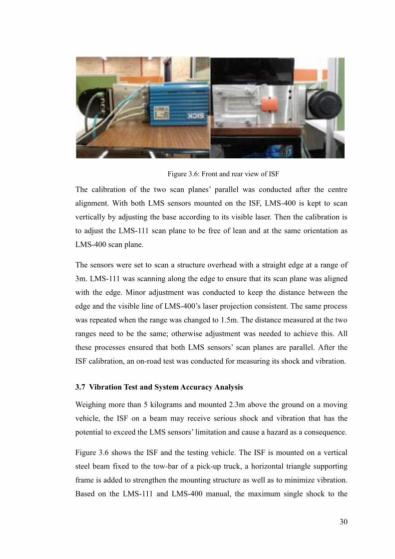
Table 3.1: LMS-111 laser beam expansion ....................................................................... 31
Table 3.2: LMS-400 gap between scans ........................................................................... 32
Table 4.1: Clearance of Three different surveying objects compared with marked
clearance ............................................................................................................................ 46
Table 4.2: IRI values for asphalt surface profiling ............................................................ 57
Table 4.3: IRI values for concrete surface profiling ......................................................... 57
Table 4.4: IRI values for gravel surface profiling ............................................................. 57
Table 5.1: Line Fitting Monte Carlo Test Results ............................................................. 65
Table 5.2: Image Matching Monte Carlo Test Results ...................................................... 70
Table 5.3: VO Final Position STD and Number of Iterations ........................................... 72

xi
LIST OF NOTATIONS 3D Three Dimensional
APB Advanced Protective Barrier
DPA Data Processing Algorithm
GPS Global Positioning System
GUI Graphical User Interface
IMU Inertial Measurement Unit
IRI International Roughness Index
ISF Integrated Sensors Frame
LADAR LAser Detection And Ranging
LMS Laser Measurement Systems
MLESAC Maximum Likelihood Estimate for SAmpling Consensus
PROSAC Progressive Sample Consensus
PURSAC PURposive Sample Consensus
PVA Position, Velocity and Attitude
RADAR Radio Detection And Ranging
RANSAC RANdom Sample Consensus
SURF Speeded Up Robust Features
VO Visual Odometry
1
CHAPTER 1 INTRODUCTION
1.1 Background and Motivation
With the development of transportation system, bridges, tunnels, urban streets and
highways become the essential components of modern transportation infrastructure.
They improve transportation capability, but make road conditions more complex.
Over-height vehicles are often involved in bridge strike accidents with serious
consequence. Bridges and tunnels have a certain clearance for each lane and it is
critical to accurately measure and mark the clearance in order to avoid this kind of
accident. Moreover, during the service life of bridges and tunnels, deformation and
road re-pavement could lower the clearance. It is essential for safety to survey road
clearance accurately and efficiently.
The condition of the road surface has a direct impact on road safety and
comfortableness. For intelligent vehicles and an intelligent transportation system, to
enable autonomous vehicles in urban environments in the future, it is necessary to
measure the road condition accurately and efficiently. The road surface profile
includes the road boundary, surface roughness, road deformation, white line (traffic
lanes division) and marks. In order to achieve satisfactory road surface condition
assessment and road assets management, it is critical to accurately profile most of the
road sections, especially in urban area.
Traditionally, bridge and tunnel clearance and road surface condition are surveyed
manually with rods and other surveying tools. During the process, surveying
personnel need to hold rods to measure the height of suspected lowest points, which
is inefficient and may introduce human errors into the measurements. This method is
not only labour and time consuming but also creates traffic disruption and is safety
hazard for workers [1].
In the past two decades, many automatic road surveying systems were designed
based on different techniques and sensors [2]-[5], such as Vision sensor, RADAR
(Radio Detection And Ranging) sensor, LADAR (LAser Detection And Ranging)
sensor, suspension sensor, and hybrid sensor. They have been applied on road
mapping, lane & boundary detection and road roughness measurement. With the

2
rapid and recent development of sensors and computers, more and more automatic
road surveying systems are now able to deliver road asset surveying results in real-
time. Automatic road profiling is a novel way of efficiently collecting critical road
condition data and performing analysis. Compared with traditional manual surveying,
automatic surveying and profiling processes have several advantages such as cost
efficiency, less risk and impact to traffic. As a consequence, a safer and more
efficient method to measure bridges and tunnels’ clearance and many other aspects
of road condition is required. This is the motivation of the proposed research.
Most automatic road surveying systems collect road assets information with a
moving vehicle. In order to obtain accurate position, velocity and attitude
information of the vehicle, sensors such as GPS, IMU and Camera are installed onto
the surveying systems. Although GPS has outstanding precision of localization in
open space, it becomes unreliable in a signals blocked area, such as in tunnels and
the city with many tall buildings. IMU is a perfect device to measure a vehicle’s
velocity, orientation and also gravitational forces, using accelerometers and
gyroscopes. However, a vital shortcoming of IMU alone is error accumulated [64],
also known ‘drift’, as time elapses, which indicates that it is accurate only for a short
time and has to be corrected frequently. Camera based visual odometry (VO) has
been demonstrated to be able to provide accurate trajectory estimation, with relative
position error ranging from 0.1% to 2% [6]. However, camera based VO suffers in
poor illumination, in which fewer features can be extracted. In the past decades,
many integrated navigation systems have been developed for improving accuracy
and robustness of PVA measurement. The shortcomings of an individual system can
be overcome by other navigation systems. Most of the systems use inertial
navigation as the main sub-system, because it is free from external disturbance.
1.2 Objectives and Scope of the Work
The objective of research is to develop a mobile surveying system with multi-
functions, such as road-boundary detection, white line detection, clearance surveying,
road roughness measurement and 3D road surface modelling.
The proposed system is designed for delivering accurate and efficient road asset
measurement and management, with real-time processing in a surveying vehicle at

3
normal driving speed. This research also investigates visual odometry using a vision
sensor (camera). This research is aimed to provide accurate real-time PVA estimation
in GPS-denied environments, such as tunnels, in which using IMU alone would
result in inadequate PVA estimation and inaccurate 3D road profiling. Hence,
combining IMU and vision data together will limit the IMU drift and reduce PVA
estimation error.
The scope of the work is focusing on a vehicle-based platform, sensor fusion, and
data processing. The proposed surveying system developed in this research is
integrated into an experiment vehicle shown in Figure 3.3. Two LADAR sensors
(LMS111and LMS400) and an IMU are mounted on an aluminium frame and then
installed at the back of the vehicle at a proper height (2300mm) for scanning
perpendicular to the vehicle moving direction. The GPS antenna and the camera are
mounted on the top of the driver’s cab. Other sensors, data collect hardware and
power system is placed at the back of the cruise vehicle.
The work of sensor data fusion consists of sensors position calibration, sensors time
synchronization and data processing for multi-function realization. The sensors time
synchronization is one of the most challenging tasks because of a different clock and
frequency of each sensor. Another major challenge of developing the proposed
system is to process LADAR range and remission data combined with other sensors’
data, in order to obtain an integrated and comprehensive road surveying and
profiling result. The system can perform road surveying at the designated speed
therefore it has no impact on normal traffic during the surveying.
1.3 Contributions
The major contributions of the thesis are as follows:
Designed and developed an automatic road surveying system to collect road
surface and surroundings data with a test vehicle driving at the road speed
limit. Data from sensors can be processed on-line with comprehensive
information recorded, processed and profiled for road assets condition
analysis and management.

4
Developed several road surveying and profiling functions, such as road
boundary detection, clearance measurement for tunnels and bridges, road
surface markers extraction, white line & traffic lane extraction, 3D model and
GUI construction and road roughness measurement. They can be utilized in
varied environments and for different purposes.
Research on Visual Odometry has been conducted for PVA estimation. A new
algorithm named PURSAC has been proposed as a major component of
Visual Odometry for outlier removal. It has demonstrated better accuracy,
robustness and efficiency compared with other methods, such as RANSAC
and MLESAC (maximum likelihood estimation sample consensus).
1.4 Thesis Outline
Chapter 2 presents a literature review of road asset surveying on road mapping, lane
and boundary detection, road roughness measurement and clearance measurement by
utilizing LADAR based technique and vision based techniques. In addition to this,
visual odometry is a key component of the system, a literature review of feature
detection and feature matching and robust estimation methods for outlier removal
has been described in detail in the second part of this chapter.
Chapter 3 presents a comprehensive description and analysis of the proposed
autonomous surveying system, which includes system architecture, system hardware,
data acquisition software, sensor data and system accuracy analysis.
Chapter 4 introduces a number of functions developed for the proposed system.
Road boundary detection and white line & traffic lane extraction are the fundamental
functions for clearance measurement of tunnels and bridges. Other functions, such as
road surface markers extraction, 3D model & GUI construction and road roughness
measurement, are designed as on-line data processing functions to deliver detailed
information of the road surface and surroundings. The information can be utilized for
road assets monitoring and management, as well as for problem analysis in the future.
Chapter 5 presents improved visual odometry, which is applied on the proposed
system. The frame structure of the proposed approach, detailed algorithm and
experimental setup are introduced, and test results are discussed. The repeatability
and efficiency of visual odometry using the proposed PURSAC and other algorithms

5
have been compared and analysed. The results indicate that the proposed method
demonstrates a great improvement on both repeatability and efficiency.
Chapter 6 concludes the summary of the presented outcomes and the outlook for
related research, as well as some potential functions, which could supplement this
proposed system in the future.
6
CHAPTER 2 LITERATURE REVIEW
2.1 Road Mapping and Surveying
Many surveying systems have been developed in the past two decades for road
mapping, lane and boundary detection, road profile or tunnel and bridge clearance
measurement. They have been based on either a single sensor, such as a LADAR
sensor, RADAR sensor, vision sensor and suspension device, or sensor fusion, such
as LADAR/vision or RADAR/vision fusion. In road lane and boundaries modeling
and prediction aspects, some methods, such as extended Kalman filtering, have
performed well in real time processing. A literature review of road mapping, lane and
boundary detection, road profile and clearance measurement is presented in detail in
the following parts.
LADAR is a remote sensing technology that measures the distance between the
sensor and a target surface, which is obtained by determining the elapsed time
between the emission of a short duration laser pulse and the arrival of the reflection
return signal [70]. The LADAR Technique has been widely applied to make high-
resolution maps with applications in geomatics, archaeology, geography, geology,
seismology, geomorphology, forestry, remote sensing and atmospheric physics [71].
It uses near-infrared light to image objects and can be used with various materials
including non-metallic objects, rocks, rain, chemical compounds, aerosols, clouds
and even single molecules [71]. In this part of the literature review, the focus is on
LADARs and their sensor fusions that have been applied to an autonomous vehicle.
2.1.1 Road Mapping Road mapping focuses on creating the geometry of a road by using images or
LADAR data. The created road mapping can be unitized for localization and road
asset management. In the past decade, many systems for road mapping have been
developed based on a vision sensor [7-10], LADAR sensor [11-13] and sensor fusion
[14-16].
In systems using a vision sensor alone, standard images are applied; others, such as
high-resolution satellite imagery, are becoming more and more frequently used as

7
they show advantages of high resolution, large coverage area and high precision on
localization. Jin [7] proposed an integrated system for automatic road mapping using
high-resolution multi-spectral satellite imagery. This system has distinguished road
models for urban areas and suburban areas. In suburban areas, roads are treated as
curvilinear and homogeneous regions with constant width and final suburban roads
centrelines are generated by integrated results from detectors by using a path search
algorithm. In urban areas in the USA, road networks consist of straight lines, which
form a grid structure. Jin then uses a spatial signature weighted Hough transform to
generate a road grid hypothesis. This system using representative test sites indicates
correctness values that range between 70% and 92%. Olson [8] presented a vision
based robust and efficient robotic mapping system, especially when dealing with
large maps or large numbers of observations. The author described an optimization
algorithm that can rapidly estimate the maximum likelihood map given a set of
observations. The proposed place recognition algorithm has demonstrated that it can
robustly handle ambiguous data. Dong [9] introduced an overview of recent
advances in multi-sensor satellite image fusion in application fields of object
identification, classification, change detection and manoeuvre targets tracking. Also
Dong [9] pointed out the most popular and effective image fusion techniques;
intensity-hue-saturation (IHS), high-pass filtering, principal component analysis
(PCA), different arithmetic combination (e.g. Brovey transform), multi-resolution
analysis-based methods (e.g. pyramid algorithm, wavelet transform), and Artificial
Neural Networks (ANNs).
A road mapping method proposed by Doucette [10] utilizes high-resolution
multispectral imagery for road extraction and mapping. Doucette presents a Self-
Supervised Road Classification (SSRC) feedback loop to automate the process of
training sample selection and refinement for a road class. SSRC demonstrates a
dramatic improvement in road extraction results by exploiting spectral content.
Although a vision based sensor for road mapping is inexpensive and can be started
quickly, it is still very hard to extract a three-dimensional road map by using the
vision sensor alone. LADAR or sensors fusion-based systems would overcome this
drawback and provide vivid 3D road maps.
8
In LADAR based systems for road mapping, Kukko [11] developed a mobile
mapping system and some computing methods for road environment modeling.
Author used LADAR based mobile mapping system to produce three dimensional
point clouds from surrounding objects. Two-dimensional point clouds are captured
from the LADAR sensor while the third dimension is the vehicle moving direction.
Lin [12] established a mini-UAV-borne LADAR system where an Ibeo Lux scanner
mounted on a small Align T-Rex 600E helicopter. The bird’s eye mini-UAV-borne
LADAR system collects point clouds data from air and validates its applicability for
fine-scale mapping, in terms of tree height estimation, pole detection, road extraction
and digital terrain model refinement. Another similar system using airborne LADAR
data to extract digital terrain models, roads and buildings is proposed by Hu [13].
The three-dimensional grid road networks are reconstructed using a sequential
Hough transformation and the building boundaries are detected by segmenting
LADAR height data. The test results based on many LADAR datasets of varying
terrain type have demonstrated robustness and effectiveness of the algorithm. Traffic
neglect of airborne LADAR based system is the most dominant aspect for road
mapping. However, the airflow has a significant impact on such a small helicopter,
sometimes causing failure of experiments. For a vehicle LADAR based system, it is
influenced by road traffic and other vehicles, but airflow has no impact.
To overcome shortcomings of applying a vision sensor and a LADAR sensor, some
researchers tried to integrate two types of sensors and deliver more accurate road
information results with less limitation. Shi [15] developed an automatic road
mapping system by fusing vehicle-based navigation data, stereo image and laser
scanning data for collecting, detecting, recognizing and positioning road objects. It
declares that the system is applicable for generating high-accuracy and high-density
three dimensional road spatial data more rapidly and less expensively. Sohn [16]
presented a new approach for automatic extraction of building footprints in an
integration of high-resolution satellite imagery and LADAR data. A laser point cloud
in 3D object space was recognized as an isolated building object and normalized
difference vegetation indices were driven from satellite imagery. The final
description of building outlines was achieved by merging convex polygons using the
binary space-partitioning tree. It states that the correctness of detection can reach up
9
to 90.1% and the overall quality can reach 80.5%. Sensors fusion, overcoming
shortcoming of individual sensor, is a vital challenge.
2.1.2 Lane and Boundary Detection
LADAR based road boundary detection [19] method is popular in recent years, not
only due to its direct distance measurement, but also its accuracy and robustness.
Wurm et al [24] proposed a novel laser based road boundary detection algorithm
with good results, however, only working on simple, flat road boundaries confines its
usage. Real-time information can be provided by radar data; Yamaguchi et al [21]
performed the test of a van-mounted radar to detect road markers. It is limited to
operating at 50 km/h, which could cause traffic congestion and affect other road
users. A few approaches [5], [11] perform mobile road mapping based on road
models, which work very well in principle; however, due to the complexity of the
modern road network, methods above may have robustness issues. W.S. Wijesoma et
al [2] introduced a method based on extended Kalman filtering for fast detection and
tracking of road curbs. However, the lack of clearance surveying and road surface
condition monitoring limits its ability for full-scale assets surveying.
Although, LADAR has better performance on accuracy and robustness compared
with vision sensors (camera), the higher cost and lower resolution are important
concerns for some researchers to turn away from LADAR, and adopt cameras
instead. M. Hu et al [18] proposed a vision based road recognition algorithm. The
algorithm is divided into two modules. The first module is to obtain road boundaries
information when the vehicle starts moving. The second module is to predict
positions of road edge when the vehicle moves at constant speed by applying
prediction knowledge. C. Guo [20] presented stereovision-based road boundary
detection for an intelligent vehicle. Both of the road boundaries are generated using
Catmull-Rom splines based on the RANSAC algorithm with varying road structure
models.
Using mono-vision for lane detection and tracking, Y. Wang et al [23] proposed a B-
snake based lane detection and tracking algorithm without any camera parameters.
The experimental result shows that the proposed method is robust against noise and
shadow. H. Lin et al [25] introduced a randomized Hough transform method to
10
detect practically useful road boundaries with straight line segments, but Dynamic
Programming (DP) has to be utilized to obtain the most likely road boundaries field
as the first priority. H. Kong et al [26] introduced a new vanishing-point-constrained
edge detection technique for detecting road boundaries, and it has been successfully
implemented and tested with 1003 general road images. However, the dependence of
ambient light affects the functionality in the real world. Surveying road assets at
night, where illumination conditions are poor, a vision recognition method may not
be applicable.
Sensors fusion, such as vision & LADAR fusion [4] [17] and vision & RADAR
fusion [22], for lane and road boundaries detection becomes a choice to researchers.
Not only does it overcome the weakness of an individual, but also improves the
accuracy of road boundaries detection results.
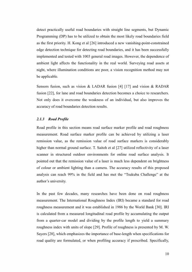
2.1.3 Road Profile
Road profile in this section means road surface marker profile and road roughness
measurement. Road surface marker profile can be achieved by utilizing a laser
remission value, as the remission value of road surface markers is considerably
higher than normal ground surface. T. Saitoh et al [27] utilized reflectivity of a laser
scanner in structured outdoor environments for online road surface analysis. It
pointed out that the remission value of a laser is much less dependent on brightness
of colour or ambient lighting than a camera. The accuracy results of this proposed
analysis can reach 99% in the field and has met the “Tsukuba Challenge” at the
author’s university.
In the past few decades, many researches have been done on road roughness
measurement. The International Roughness Index (IRI) became a standard for road
roughness measurement and it was established in 1986 by the World Bank [30]. IRI
is calculated from a measured longitudinal road profile by accumulating the output
from a quarter-car model and dividing by the profile length to yield a summary
roughness index with units of slope [29]. Profile of roughness is presented by M. W.
Sayers [28], which emphasizes the importance of base-length when specifications for
road quality are formulated, or when profiling accuracy if prescribed. Specifically,
11
the accuracy of high-speed profiling systems should be specified according to base-
length. IRI values can be determined either by applying dynamic motion using
suspensions or by laser/inertial profile meters. Recently, a one-wheel trailer was
developed for estimating the road surface profile based on the vehicle dynamics
motion using suspensions and trajectory control systems [5]. However, it can only
survey a tiny fraction of a single traffic lane; conditions of the rest of the road are
unreached.
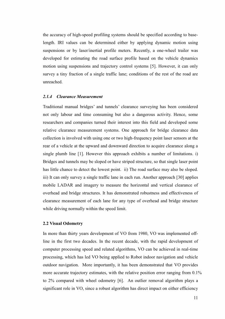
2.1.4 Clearance Measurement
Traditional manual bridges’ and tunnels’ clearance surveying has been considered
not only labour and time consuming but also a dangerous activity. Hence, some
researchers and companies turned their interest into this field and developed some
relative clearance measurement systems. One approach for bridge clearance data
collection is involved with using one or two high-frequency point laser sensors at the
rear of a vehicle at the upward and downward direction to acquire clearance along a
single plumb line [1]. However this approach exhibits a number of limitations. i)
Bridges and tunnels may be sloped or have striped structure, so that single laser point
has little chance to detect the lowest point. ii) The road surface may also be sloped.
iii) It can only survey a single traffic lane in each run. Another approach [30] applies
mobile LADAR and imagery to measure the horizontal and vertical clearance of
overhead and bridge structures. It has demonstrated robustness and effectiveness of
clearance measurement of each lane for any type of overhead and bridge structure
while driving normally within the speed limit.
2.2 Visual Odometry In more than thirty years development of VO from 1980, VO was implemented off-
line in the first two decades. In the recent decade, with the rapid development of
computer processing speed and related algorithms, VO can be achieved in real-time
processing, which has led VO being applied to Robot indoor navigation and vehicle
outdoor navigation. More importantly, it has been demonstrated that VO provides
more accurate trajectory estimates, with the relative position error ranging from 0.1%
to 2% compared with wheel odometry [6]. An outlier removal algorithm plays a
significant role in VO, since a robust algorithm has direct impact on either efficiency

12
or accuracy of systems. In the following, a comprehensive review of outlier removal
algorithm is presented, which was established thirty years ago.
RANSAC is still the fundamental algorithm for robust model fitting and outlier
removal for the past thirty years. The principle steps of RANSAC can be
summarized as: 1) randomly select a set of samples from all samples; 2) fit a model
hypotheses with the selected set of samples; 3) compute the distance of all other
points to this model; 4) construct the inliers set with a distance threshold and
compare its inliers count to the previous highest one and store the results. Steps 1 to
4 are repeated until a pre-set threshold of iterations is reached. The set with
maximum number of inliers is chosen, all these inliers are used for model parameter
estimation [31].
Assuming all the samples have the same outlier possibility ε, and ignoring the impact
of sampling noise, RANSAC follows a random sampling paradigm. Fundamentally
it is a stochastic algorithm without deterministic guarantees of finding the global
maximum of the likelihood. A success rate p is the level of confidence of finding a
consensus subset, which is a function of ε, the number of iterations to be conducted
N and the number of samples in a subset s [32].
(2.1)
For the sake of robustness, in many practical implementations N is usually
multiplied by a factor of ten, which increases computational costs [31]. Without prior
knowledge of ε, commonly the implementations of RANSAC estimate ε adaptively,
iteration after iteration.
In practice, sampling always has noise and ε may be different for each sample. By
analysing the difference of ε, it has large potential for optimizing sample subsets
selection and improving model fitting performance. As an example, assuming a
required success rate p is 99% and a dataset with outlier rate ε = 50%, according to
(2.1), the number of iterations N is 16 for s = 2 (line fitting), 145 and 587 for s = 5
and 7 (visual odometry). ε still is 50% for the entire dataset, but ε = 20% for a
special part of the dataset. If sample subsets are selected only from this part of the

13
dataset, N is just 5, 12 and 20 for s = 2, 5 and 7 respectively. This leads to one of the
strategies in PURSAC, which will be detailed in the line-fitting example.
RANSAC estimator[32] and its variants [33-37] are popular methods for eliminating
outliers and fundamental matrix estimation in computer vision. MLESAC was
established by Torr and Zisserman [38] and adopts the same sampling strategy as
RANSAC to generate putative solutions, but chooses the solution to maximize the
likelihood rather than just the number of inliers. GroupSAC [35] derived by Kai
recently performed well in dealing with the cases of high outlier ratios. However,
image segmentation for group sampling increases computational costs. Capel [40]
proposed a statistical bail-out test for RANSAC that permits the scoring process be
terminated early and achieves computational savings. Such methods developed on
the basis of RANSAC. However, they share a common weakness of imprecision.
This is due to the fact that the tentative features set is randomly chosen from the
entire data set, which may result in large differences of model estimates in each trial.
For most model fitting tasks, two types of measurement errors must be considered:
small errors (noise) and blunders (outlier) [35]. If the sensitivity analysis of a model
against the noise of selected sample sets can be conducted and/or the patterns of the
measurement errors can be found, then a method better than random selection can be
found which can reduce the effect of measurement noise and/or outlier for model
fitting. This is the fundamental principle of the new paradigm for robust outlier
removal and model fitting - purposive sample consensus (PURSAC). Although in
theory PURSAC is just a qualitative guidance, the implementation of it usually needs
quantitative analysis to design executable rules for purposive sample set selection.
In this research, PURSAC is detailed with the line-fitting example and then applied
for visual odometry (VO), which is the process of estimating egomotion of an agent
(e.g. vehicle, human or robot) using single or multiple cameras attached to it. VO
operates by incrementally estimating the pose of the agent through examination of
the changes that movement induces on the images of its onboard cameras [31].
Nowadays most VO implementations are feature based, which use salient and
repeatable features extracted and matched across the captured images. Not only VO,
but also many other computer vision applications, such as structure from motion and
14
image registration etc. require a more efficient and robust method to be developed
for eliminating outliers in the matched features and improving the precision and
consistency of fundamental matrix estimation.
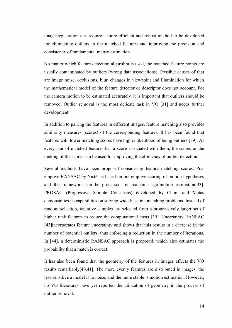
No matter which feature detection algorithm is used, the matched feature points are
usually contaminated by outliers (wrong data associations). Possible causes of that
are image noise, occlusions, blur, changes in viewpoint and illumination for which
the mathematical model of the feature detector or descriptor does not account. For
the camera motion to be estimated accurately, it is important that outliers should be
removed. Outlier removal is the most delicate task in VO [31] and needs further
development.
In addition to pairing the features in different images, feature matching also provides
similarity measures (scores) of the corresponding features. It has been found that
features with lower matching scores have higher likelihood of being outliers [39]. As
every pair of matched features has a score associated with them, the scores or the
ranking of the scores can be used for improving the efficiency of outlier detection.
Several methods have been proposed considering feature matching scores. Pre-
emptive RANSAC by Nistér is based on pre-emptive scoring of motion hypotheses
and the framework can be processed for real-time ego-motion estimation[33].
PROSAC (Progressive Sample Consensus) developed by Chum and Matas
demonstrates its capabilities on solving wide-baseline matching problems. Instead of
random selection, tentative samples are selected from a progressively larger set of
higher rank features to reduce the computational costs [39]. Uncertainty RANSAC
[43]incorporates feature uncertainty and shows that this results in a decrease in the
number of potential outliers, thus enforcing a reduction in the number of iterations.
In [44], a deterministic RANSAC approach is proposed, which also estimates the
probability that a match is correct.
It has also been found that the geometry of the features in images affects the VO
results remarkably[40,41]. The more evenly features are distributed in images, the
less sensitive a model is to noise, and the more stable is motion estimation. However,
no VO literatures have yet reported the utilization of geometry in the process of
outlier removal.
15
Applied in VO, existing algorithms mentioned above are mainly focused on reducing
computational costs, but dismiss precision and reliably. Without considering features
ranking and/or geometry, performance improvement of these algorithms is usually
limited and unstable. The proposed PURSAC concerns both features’ geometry and
matching score/ranking in sample sets selection so as to improve fundamental matrix
estimation. In endeavouring to increase processing speed, the proposed PURSAC
also improves efficiency and precision, resulting in a robust and reliable VO.
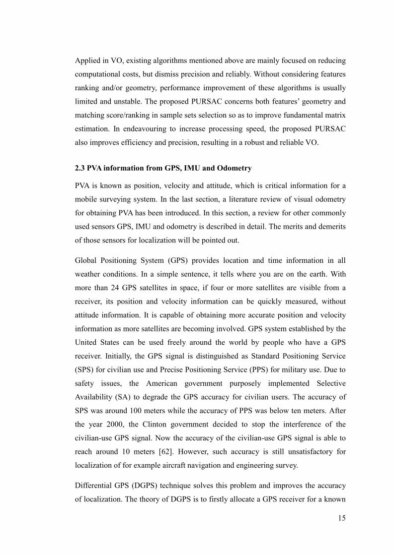
2.3 PVA information from GPS, IMU and Odometry
PVA is known as position, velocity and attitude, which is critical information for a
mobile surveying system. In the last section, a literature review of visual odometry
for obtaining PVA has been introduced. In this section, a review for other commonly
used sensors GPS, IMU and odometry is described in detail. The merits and demerits
of those sensors for localization will be pointed out.
Global Positioning System (GPS) provides location and time information in all
weather conditions. In a simple sentence, it tells where you are on the earth. With
more than 24 GPS satellites in space, if four or more satellites are visible from a
receiver, its position and velocity information can be quickly measured, without
attitude information. It is capable of obtaining more accurate position and velocity
information as more satellites are becoming involved. GPS system established by the
United States can be used freely around the world by people who have a GPS
receiver. Initially, the GPS signal is distinguished as Standard Positioning Service
(SPS) for civilian use and Precise Positioning Service (PPS) for military use. Due to
safety issues, the American government purposely implemented Selective
Availability (SA) to degrade the GPS accuracy for civilian users. The accuracy of
SPS was around 100 meters while the accuracy of PPS was below ten meters. After
the year 2000, the Clinton government decided to stop the interference of the
civilian-use GPS signal. Now the accuracy of the civilian-use GPS signal is able to
reach around 10 meters [62]. However, such accuracy is still unsatisfactory for
localization of for example aircraft navigation and engineering survey.
Differential GPS (DGPS) technique solves this problem and improves the accuracy
of localization. The theory of DGPS is to firstly allocate a GPS receiver for a known

16
point as a reference station, which has already been accurately determined, and
simultaneously execute GPS surveying between the reference station and the moving
object. According to the accuracy of reference station coordinates, distance
correction from reference station to satellite can be worked out and send out at the
same time. The moving object receives the GPS signal, and simultaneously receives
distance correction from the reference station. Based on distance correction,
accuracy of localization can be improved [63].
Inertial Measurement Unit (IMU) is an electronic device that measures an object’s
velocity, orientation and gravitational forces using accelerometers, gyroscopes and
magnetometers. IMU is the core of inertial navigation systems, which has been
widely used in aircraft, watercraft and the military. The data collected from IMU can
be used for tracking an object’s position using a method called Dead Reckoning. In a
navigation system, data extracted from IMU to computer is utilized to calculate
current position based on velocity and time.
The advantage of using IMUs is that it is a standalone device, which is not able to be
interrupted externally. However, a vital disadvantage of using IMUs is that they
suffer from accumulated error [64]. Because, the object’s current position calculated
from IMUs is continuously being added to the previous calculated position, errors in
each measurement, although are small, they are still accumulated and getting larger.
This is also known as ‘drift’. In a word, although IMUs are free from external
disturbance, their drawback of error accumulation has to be corrected by information
from other navigation sensors, such as GPS and Odometry.
Two types of odometry are investigated in this research. The first one is visual
odometry, which has been introduced in the last section of the Literature Review.
Another one is wheel odometry that uses data from a rotary encoder to work out the
travelling distance over time, which has been applied on wheeled robots and vehicles.
At the current stage, wheel odometry is more often used in the proposed system due
to its consistency.
Figure 2.1 shows a vehicle moving from time state T to state T+1. To work out the
position change and orientation of the vehicle across a given time span (T to T+1),
linear distance DR and DL has to be calculated in the first place (calculated from the

17
number of ticks from the encoders and the diameter of the wheels) [65]. The
orientation of the T+1 state is calculated by:
OT+1 = OT + (DR - DL) / W (2.2)
The distance between state T and T+1 is:
DT,T+1 = (DR + DL) / 2 (2.3)
In order to build a map of vehicle travelling, the Cartesian coordinate of state T+1 is
calculated as [65]:
XT+1 = XT + DT,T+1cos(OT+1) (2.4)
YT+1 = YT + DT,T+1sin(OT+1) (2.5)
Figure 2.1: Schematic diagram of vehicle moving in time state T and state T+1 [65] Although wheel odometry operates easily, the accuracy of wheel odometry is
strongly affected by roughness and the slope of the road surface. The worse the road
conditions the larger error that will be presented. Cheng [66] revealed that when the
wheeled system travelled on a rock surface, the error of using wheel odometry
becomes increasingly large as traveling distance increases. It becomes up to 50 times
larger than the error of using visual odometry on such a surface.

18
By looking at three types of navigation sensors GPS, IMU and Odometry, each of
them has advantages, but disadvantages are also apparent. Hence, many researchers
[67-69] turned to investigate sensor fusion in order to supplement the drawback of
individual sensors. By taking GPS and IMU fusion as an example, Francois [67]
developed a GPS/IMU based multi-sensor fusion algorithm, which increases the
reliability of the system by bringing context into consideration. Incorrect data from
GPS (GPS data is unreliable under some circumstances) is rejected using contextual
information. Besides, to resolve the problem of an unreliable signal from GPS and
drift of IMU over time, the author proposed a multi-sensor Kalman Filter directly
with the acceleration of IMU. This algorithm has potential to add a high number of
sensors without modifying the structure. This sensor fusion algorithm has presented
measured reliability and flexibility for localisation of an object.
In the section, both advantages and disadvantages for PVA acquisition from GPS,
IMU and Odometry have been reviewed. In the same way as many other researches,
this study has preferred using multi-sensors fusion for obtaining PVA information. It
combines all the merits of different sensors to deliver more accurate PVA results.

19
CHAPTER 3 AUTONOMOUS SURVEY SYSTEM
3.1 Introduction This chapter gives a comprehensive description of the proposed autonomous road
surveying system as well as the reasons for constructing the system in this
particular way. The proposed system is a unique design for the multi-purposes of
surveying, including Clearance Surveying, Road Boundary Detection, White line
Detection, Road Surface Markers Extraction and Road Roughness Measurement.
More importantly, the experimental vehicle is designed for people driving at the road
speed limit and to deliver accurate on-line processing results. The system
architecture (3.2) introduces all the sensors (IMU, GPS, odometer, LADAR, and
camera) and indicates how the proposed system works. The system hardware (3.3)
provides the information of sensors installation and their connection interfaces. The
tasks performed by data acquisition software are listed in 3.4. The next three sections
are about sensor’s data, ISF Calibration and Vibration Test & system accuracy
analysis.
3.2 System Architecture
The surveying system is specifically designed for road surface and surroundings
profiling. From sensors selection to their location and installation, the proposed
surveying system has significant differences to other systems. The significant
advantage of the proposed surveying system is that it performs multi-functions, such
as road clearance measurement, road surface profiling, 3D structure modeling, road
boundary detection and road roughness measurement, at normal drive speed in urban
streets. Meanwhile, data collected by sensors has less chance of being blocked by
other vehicles.
In order to develop a robust and efficient road surveying system that can provide
road profiles in all circumstance, multi-sensor integration is the optimal approach.
The thread in designing the proposed system is to build a versatile, multipurpose
platform for road surveying. Due to the complexity of multi-sensor measurements, a
proper sensor fusion framework needs to be developed with accurate surveying

20
procedures, reliable modelling and quality control algorithms. The proposed multi-
sensor integrated mobile surveying system consists of two laser sensors (LADAR),
GPS, IMU, odometer and camera, as shown in Figure 3.1.
Figure 3.1: Multi-sensors fusion system architecture
IMU is selected as the reference navigation sensor because it can provide continuous
PVA data with time-accumulated drift. The odometer can measure vehicle speed and
mileage. GPS is a time-invariant navigation system with assured position and
velocity measurement in open space, which can be used to correct the IMU and
odometer errors. Most importantly, GPS’s accurate clock is used for the sensors’ time
synchronization. LADAR is the main surveying component of the proposed system.
Range and remission data are collected by LADAR and fused with other sensors’
measurements to perform all the system’s tasks. The camera records the road’s
characteristics as a visual reference, as well as trajectory from visual odometry
processing.
3.2.1 PVA Acquisition
PVA information plays a significant role in the system. As shown in Figure 3.1, PVA
is extracted and processed from the fusion of GPS, IMU and Odometry data. GPS
has been widely applied in navigation, such as aircraft navigation, vehicle navigation,
weapon navigation, and localization, such as in a vehicle burglary-resisting system
and automatic drive system. The following is a list of reasons why it is popular to the
public: 1) 24 hours working, it is able to operate in all kinds of weather; 2) High
coverage area (98%) of GPS around the World; 3) High accuracy of 3D localization;
21
4) very high efficiency; 5) mobile localization device. However, a significant
drawback of GPS exists. In some blocked area, such as in tunnels, the GPS signal is
hard to be received, which brings trouble to users. Besides, when driving on an urban
road surrounded by tall buildings, the GPS signal becomes unreliable and it changes
frequently, which causes confusion to users.
In an open area, INS and GPS fusion are adopted to obtain PVA information. INS
has a vital drawback of drifting over time. Although the precision of GPS is good in
an open environment, it is very sensitive to the environment. Hence, GPS/INS fusion
would overcome drawbacks of each other. In the surveying system, INS provides
continuous attitude information. By applying Kalman Filter and GPS data, INS
results are recalculated and drift is minimised at each state.
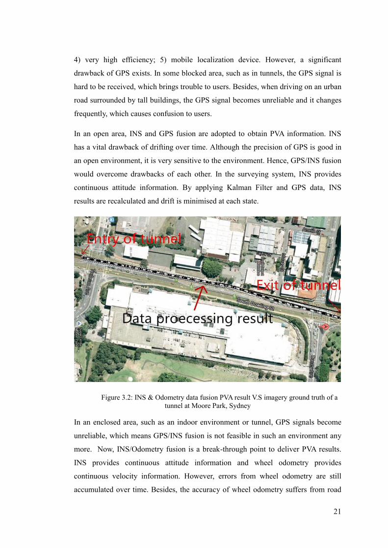
Figure 3.2: INS & Odometry data fusion PVA result V.S imagery ground truth of a tunnel at Moore Park, Sydney
In an enclosed area, such as an indoor environment or tunnel, GPS signals become
unreliable, which means GPS/INS fusion is not feasible in such an environment any
more. Now, INS/Odometry fusion is a break-through point to deliver PVA results.
INS provides continuous attitude information and wheel odometry provides
continuous velocity information. However, errors from wheel odometry are still
accumulated over time. Besides, the accuracy of wheel odometry suffers from road

22
condition which will bring larger error to PVA results. In Figure 3.2, comparing with
PVA result of INS & odometry data fusion and imagery ground truth of a tunnel at
Moore Park, Sydney, the drift does exist. In Chapter 5, visual odometry is introduced
for the reasons of 1) more accurate PVA results, 2) no reliance on road condition,
which has a larger potential for integrating with INS.
3.2.2 Surveying Functions
The proposed system is designed for multi-functions purposes. Combining PVA
information and LADARs range & remission data, functions such as road clearance
surveying, road surface profiling, 3D structure modelling, road boundary detection
and road roughness measurement can be achieved. These are also the outputs of the
surveying system as indicated in Figure 3.1.
To start with the first function, automatic clearance surveying is applied to bridges
and tunnels, which is aimed to replace traditional manual clearance surveying and
deliver accurate survey results. Remission values from LADARs are firstly applied
for white line detection and lane division. Although, a white line has significant
higher remission value, the remission value of others, such as a sewage cover and
undried water, are still hard to distinguish from a white line remission value. Hence,
a fuzzy logic filter is developed for filtering this noise. Then, the road surface and
ceiling of tunnels or bridges is modelled according to LADARs range data. Finally,
clearance within each lane is calculated and it is perpendicular to the road surface.
Road surface profiling is another output for surface marker extraction. It can be used
for road markers healthiness determination. LADARs remission and range data
becomes involved in surface marker processing. As the remission value of road
surface markers is distinguishable, road surface markers can be extracted easily.
Road boundary detection is a frequent topic in related research and applications. The
importance of achieving road boundary detection is to distinguish driveway and non-
motor way. LADAR sensor’s range data is used in this part. Most importantly, two
ends of a road boundary can be used as a significant condition for lane division,
especially, when white lines are indistinct.

23
Road roughness measurement as a one of output is utilized for road healthiness
determination. LADARs range data and INS data are applied in this function where
INS data is used for vehicle vibration compensation. As indicating in Figure 3.1,
PVA information is obtained from local fusion 1. By combining PVA with other
output functions, a detailed 3D road assets structure can be successfully profiled.
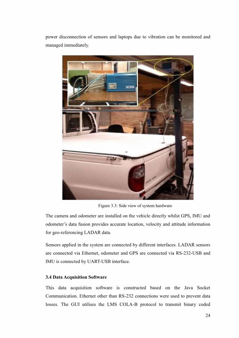
3.3 System Hardware
The hardware component consists of LADAR laser range sensors, IMU sensor, GPS
sensor, odometer and mechanical support structure. The platform was designed to let
the LADAR sensors scan the road assets cross-sections. As shown in Figure 3.3,
both laser sensors are mounted on an aluminum integrated sensors frame (ISF),
which is then installed at the back of a vehicle at a proper height (2300 mm), for
scanning perpendicular to the vehicle moving direction. An ‘A’ shape steel is
connected between the vehicle body and the steel pole at the back of vehicle, in order
to reduce vibration. Due to its wider scan angle, the LMS-111 is on the right side of
the frame, which allows it to scan from the left-lane to right-lane for both the ground
and overhead objects while driving along the left-lane. Its remission data is also
collected for lane detection. The LMS-400 is mounted on the front of the ISF, which
takes the full advantages of its fast scan frequency and accurate range measurement
to detect smaller objects whilst the vehicle is travelling at high speed.
Aluminium integrated sensors frame is designed using AutoCAD (APPENDIX D).
The reason for constructing such frame is to integrate LADARs and IMU into the
same body which offers greater convenience of system calibration. Furthermore, the
ISF has been designed for multi-proposals. The current proposal is presented as
Figure 3.5 indicates and the vehicle drives at the most left lane. Another proposal is
to rotate LMS111 and LMS400 180 degrees so that the vehicle is able to drive in the
most right lane and deliver the same surveying results.
A power source module is embedded at the back of vehicle, which is capable of
providing charging to all sensors and laptops for a whole day experimental test. A
plug socket is placed at the back seat of the vehicle, which is connected to the power
source. Sensors’ power cables are wired along ‘A’ shape steel and gathered together
to the back seat of vehicle. Finally, they are all connected to the plug socket. Any
24
power disconnection of sensors and laptops due to vibration can be monitored and
managed immediately.
Figure 3.3: Side view of system hardware
The camera and odometer are installed on the vehicle directly whilst GPS, IMU and
odometer’s data fusion provides accurate location, velocity and attitude information
for geo-referencing LADAR data.
Sensors applied in the system are connected by different interfaces. LADAR sensors
are connected via Ethernet, odometer and GPS are connected via RS-232-USB and
IMU is connected by UART-USB interface.
3.4 Data Acquisition Software This data acquisition software is constructed based on the Java Socket
Communication. Ethernet other than RS-232 connections were used to prevent data
losses. The GUI utilises the LMS COLA-B protocol to transmit binary coded

25
messages, and maximises the communication speed [47]. The binary messages are
then converted into decimal and stored into .mat files. The .mat files (a Matlab
readable file) can be processed directly in the following Data Processing Algorithm
(DPA) developed with MATLAB.
SOPAS is the original software to connect to LMS sensors [46]. However, it has
limited functionality for scan data plotting and recording [47]. Based on tests results,
SOPAS takes 67 milliseconds to record each scan data, which is roughly 15 Hz.
Compared with the 50 Hz scan frequency of LMS-111 and 370 Hz of LMS-400,
SOPAS’s recording rate is very limited. For this reason, a graphic user interface
(GUI) for the sensors control and data acquisition was developed as shown in Figure
3.4. The proposed GUI is designed for controlling sensors and road condition
monitoring in real-time. All sensors and laptops are connected to a power source
which is embedded in the experimental vehicle.
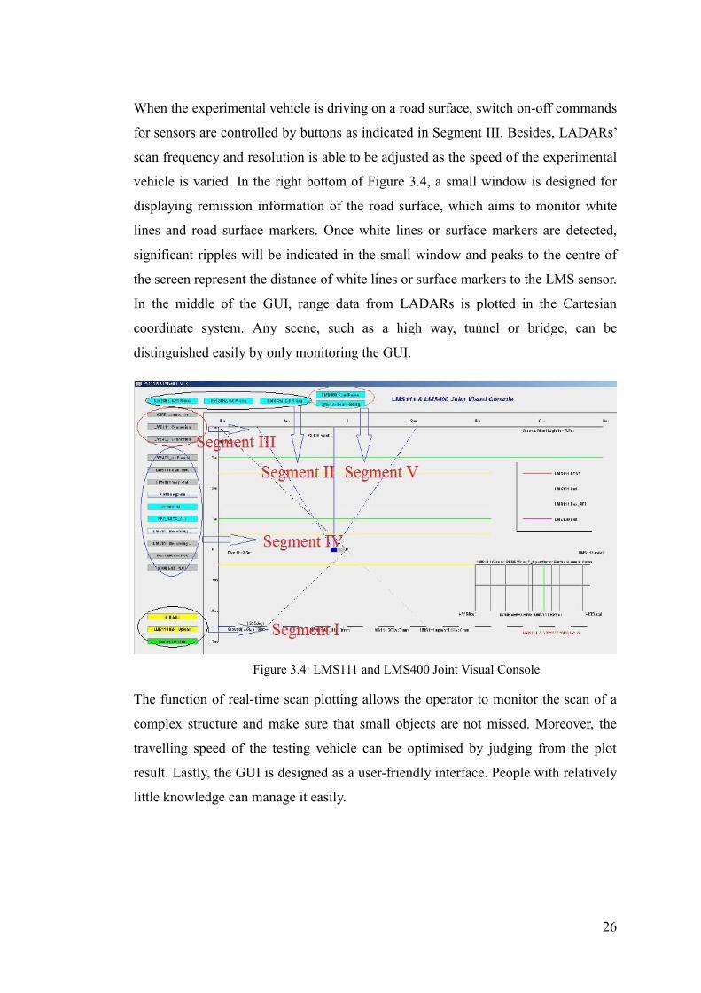
Control console is divided into five segments as red colour indicates in Figure 3.4. It
performs well in data acquisition, recording and system robustness. Segment I
provides detailed instruction of how to operate this GUI and all sensors. Segment II
functions as a tuner for LADARs and IMU frequency adjustment. The default
frequency of LMS111 and LMS400 is 50Hz with resolution angle 0.5 degree and
370 Hz with resolution angle 0.25 degree respectively. By pressing the tuner buttons
from Segment II, the frequency of LMS111 can be adjusted to 25 Hz with resolution
angle 0.25 degree and the frequency of LMS 400 can be varied from 370Hz to
500Hz with resolution angle 0.3636 degree. After becoming familiar with GUI
instruction and sensors frequency tuning, sensors now are able to be connected by
pressing buttons from Segment III. Input LADARs’ data will be plotted in the middle
of the GUI in real time. If surveying target is approaching, functions in Segment IV
can be activated for data recording, while when the surveying task is finished,
buttons in Segment IV can be used for data collection termination, finally saving
data in to a text file. For further data analysis, functions in Segment V are managed
for translating text files to .mat files which will be processed directly in the Data
Processing Algorithm (DPA) with Matlab.
26
When the experimental vehicle is driving on a road surface, switch on-off commands
for sensors are controlled by buttons as indicated in Segment III. Besides, LADARs’
scan frequency and resolution is able to be adjusted as the speed of the experimental
vehicle is varied. In the right bottom of Figure 3.4, a small window is designed for
displaying remission information of the road surface, which aims to monitor white
lines and road surface markers. Once white lines or surface markers are detected,
significant ripples will be indicated in the small window and peaks to the centre of
the screen represent the distance of white lines or surface markers to the LMS sensor.
In the middle of the GUI, range data from LADARs is plotted in the Cartesian
coordinate system. Any scene, such as a high way, tunnel or bridge, can be
distinguished easily by only monitoring the GUI.
Figure 3.4: LMS111 and LMS400 Joint Visual Console
The function of real-time scan plotting allows the operator to monitor the scan of a
complex structure and make sure that small objects are not missed. Moreover, the
travelling speed of the testing vehicle can be optimised by judging from the plot
result. Lastly, the GUI is designed as a user-friendly interface. People with relatively
little knowledge can manage it easily.

27
3.5 Sensors’ Data
3.5.1 Navigation Data
Navigation data from three sensors (IMU, GPS and odometer) is processed in local
fusion algorithm 1, for data synchronization and integration. When the system is
surveying in an open area with reliable GPS satellite signal, location information is
extracted from the GPS sensor, and used to correct IMU and odometer drift. When
the system is in weak or GPS denied environments, such as in tunnels or under
bridges, navigation data can be extracted from IMU and odometer. The navigation
data is used to derive position and attitude information for each surveyed road assets.
Provided by IMU sensor, attitude data is used to transform LADAR 2D range data
into spatial coordinates for 3D modelling. Attitude data includes Euler angles, 6
degree of freedom (DOF) acceleration data and quaternion. Position data is provided
by both GPS and odometer if the GPS signals are strong. Under circumstances such
as tunnel surveying where GPS signals are blocked, position data is provided by
odometer and IMU trajectory. Position data is important for road 3D modelling, for
the determinate of the length of road assets.
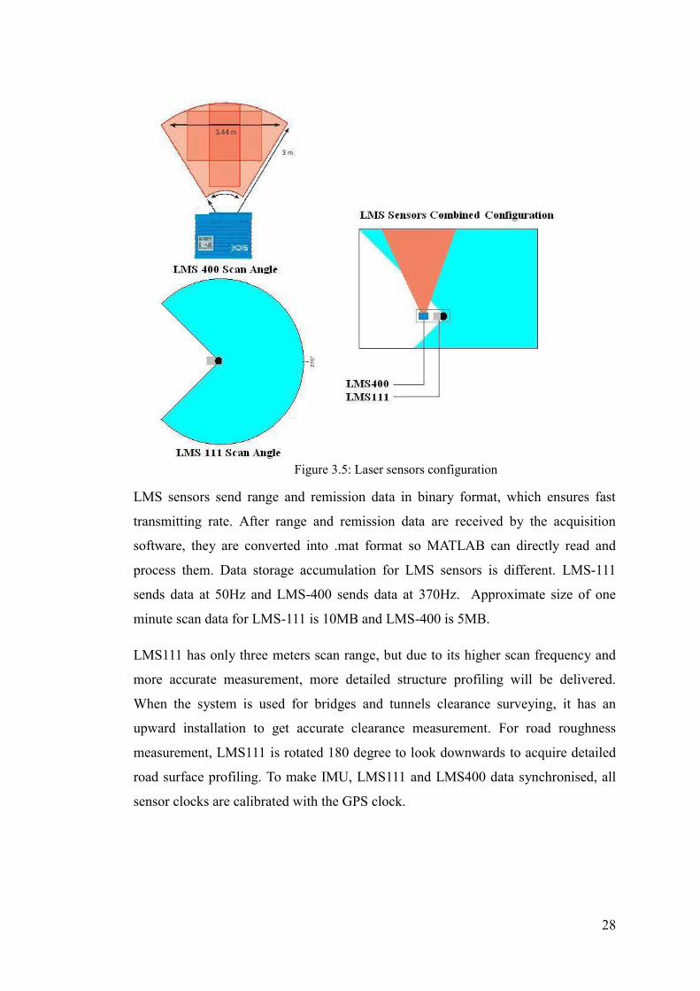
3.5.2 LADAR Range and Remission Data
LADAR range data is measured by two different SICK Laser Measurement System
(LMS) sensors, LMS-111 and LMS-400. LMS-111 scans at 50 Hz over 270º while
LMS-400 scans at 370 Hz over 70º as shown in Figure 3.5. Range data is the most
important data in this system since road surface profiles can be extracted from them.
Remission here is defined as the capability of a material to reflect the light back.
Remission data generated by the LMS-111 are acquired together with the range data.
The road surface profile is extracted based on the remission data. The traffic divide-
line (white line) has a significantly higher remission value than the road surface. As a
consequence the system can monitor the white lines by judging their remission value.
Remission data is also used for extracting traffic-lanes so as to determine the
clearance for each traffic lane.
28
Figure 3.5: Laser sensors configuration
LMS sensors send range and remission data in binary format, which ensures fast
transmitting rate. After range and remission data are received by the acquisition
software, they are converted into .mat format so MATLAB can directly read and
process them. Data storage accumulation for LMS sensors is different. LMS-111
sends data at 50Hz and LMS-400 sends data at 370Hz. Approximate size of one
minute scan data for LMS-111 is 10MB and LMS-400 is 5MB.
LMS111 has only three meters scan range, but due to its higher scan frequency and
more accurate measurement, more detailed structure profiling will be delivered.
When the system is used for bridges and tunnels clearance surveying, it has an
upward installation to get accurate clearance measurement. For road roughness
measurement, LMS111 is rotated 180 degree to look downwards to acquire detailed
road surface profiling. To make IMU, LMS111 and LMS400 data synchronised, all
sensor clocks are calibrated with the GPS clock.
29
3.5.3 Image Data
Image data from a camera mounted on the top of the vehicle’s cab is stored in jpeg-
format and named with each surveyed road assets. General road information, such as
name, clearance signs and visual conditions is captured in image data with 800×600
pixels and frame frequencies up to 24Hz.
The significance of recording image data is to serve as a guideline for the data
processing algorithm and is used to compare processing results with the real road
segments. Moreover, images can be also utilised as an input stream for visual
odometry in order to obtain accurate PVA estimation while combining with IMU.
Detailed description of imaged based VO is presented in Chapter 6.
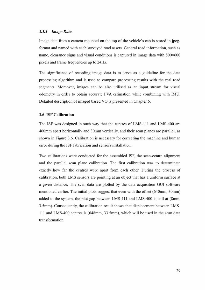
3.6 ISF Calibration
The ISF was designed in such way that the centres of LMS-111 and LMS-400 are
460mm apart horizontally and 30mm vertically, and their scan planes are parallel, as
shown in Figure 3.6. Calibration is necessary for correcting the machine and human
error during the ISF fabrication and sensors installation.
Two calibrations were conducted for the assembled ISF, the scan-centre alignment
and the parallel scan plane calibration. The first calibration was to determinate
exactly how far the centres were apart from each other. During the process of
calibration, both LMS sensors are pointing at an object that has a uniform surface at
a given distance. The scan data are plotted by the data acquisition GUI software
mentioned earlier. The initial plots suggest that even with the offset (640mm, 30mm)
added to the system, the plot gap between LMS-111 and LMS-400 is still at (8mm,
3.5mm). Consequently, the calibration result shows that displacement between LMS-
111 and LMS-400 centres is (648mm, 33.5mm), which will be used in the scan data
transformation.
30
Figure 3.6: Front and rear view of ISF
The calibration of the two scan planes’ parallel was conducted after the centre
alignment. With both LMS sensors mounted on the ISF, LMS-400 is kept to scan
vertically by adjusting the base according to its visible laser. Then the calibration is
to adjust the LMS-111 scan plane to be free of lean and at the same orientation as
LMS-400 scan plane.
The sensors were set to scan a structure overhead with a straight edge at a range of
3m. LMS-111 was scanning along the edge to ensure that its scan plane was aligned
with the edge. Minor adjustment was conducted to keep the distance between the
edge and the visible line of LMS-400’s laser projection consistent. The same process
was repeated when the range was changed to 1.5m. The distance measured at the two
ranges need to be the same; otherwise adjustment was needed to achieve this. All
these processes ensured that both LMS sensors’ scan planes are parallel. After the
ISF calibration, an on-road test was conducted for measuring its shock and vibration.
3.7 Vibration Test and System Accuracy Analysis
Weighing more than 5 kilograms and mounted 2.3m above the ground on a moving
vehicle, the ISF on a beam may receive serious shock and vibration that has the
potential to exceed the LMS sensors’ limitation and cause a hazard as a consequence.
Figure 3.6 shows the ISF and the testing vehicle. The ISF is mounted on a vertical
steel beam fixed to the tow-bar of a pick-up truck, a horizontal triangle supporting
frame is added to strengthen the mounting structure as well as to minimize vibration.
Based on the LMS-111 and LMS-400 manual, the maximum single shock to the
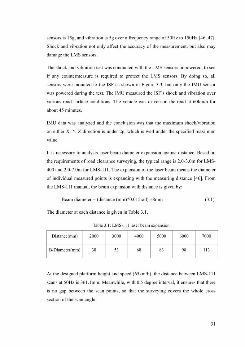
31
sensors is 15g, and vibration is 5g over a frequency range of 50Hz to 150Hz [46, 47].
Shock and vibration not only affect the accuracy of the measurement, but also may
damage the LMS sensors.
The shock and vibration test was conducted with the LMS sensors unpowered, to see
if any countermeasure is required to protect the LMS sensors. By doing so, all
sensors were mounted to the ISF as shown in Figure 3.3, but only the IMU sensor
was powered during the test. The IMU measured the ISF’s shock and vibration over
various road surface conditions. The vehicle was driven on the road at 60km/h for
about 45 minutes.
IMU data was analyzed and the conclusion was that the maximum shock/vibration
on either X, Y, Z direction is under 2g, which is well under the specified maximum
value.
It is necessary to analysis laser beam diameter expansion against distance. Based on
the requirements of road clearance surveying, the typical range is 2.0-3.0m for LMS-
400 and 2.0-7.0m for LMS-111. The expansion of the laser beam means the diameter
of individual measured points is expanding with the measuring distance [46]. From
the LMS-111 manual, the beam expansion with distance is given by:
Beam diameter = (distance (mm)*0.015rad) +8mm (3.1)
The diameter at each distance is given in Table 3.1.
Table 3.1: LMS-111 laser beam expansion
Distance(mm) 2000 3000 4000 5000 6000 7000
B-Diameter(mm) 38 53 68 83 98 113
At the designed platform height and speed (65km/h), the distance between LMS-111
scans at 50Hz is 361.1mm. Meanwhile, with 0.5 degree interval, it ensures that there
is no gap between the scan points, so that the surveying covers the whole cross
section of the scan angle.
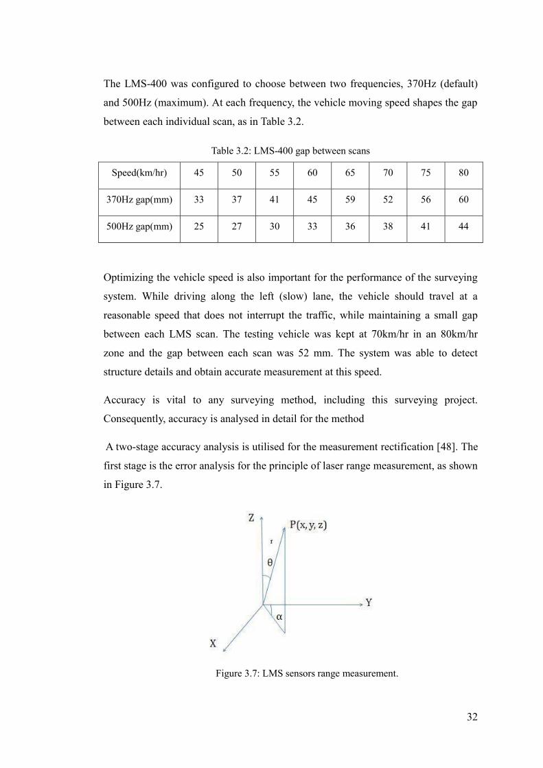
32
The LMS-400 was configured to choose between two frequencies, 370Hz (default)
and 500Hz (maximum). At each frequency, the vehicle moving speed shapes the gap
between each individual scan, as in Table 3.2.
Table 3.2: LMS-400 gap between scans
Speed(km/hr) 45 50 55 60 65 70 75 80
370Hz gap(mm) 33 37 41 45 59 52 56 60
500Hz gap(mm) 25 27 30 33 36 38 41 44
Optimizing the vehicle speed is also important for the performance of the surveying
system. While driving along the left (slow) lane, the vehicle should travel at a
reasonable speed that does not interrupt the traffic, while maintaining a small gap
between each LMS scan. The testing vehicle was kept at 70km/hr in an 80km/hr
zone and the gap between each scan was 52 mm. The system was able to detect
structure details and obtain accurate measurement at this speed.
Accuracy is vital to any surveying method, including this surveying project.
Consequently, accuracy is analysed in detail for the method
A two-stage accuracy analysis is utilised for the measurement rectification [48]. The
first stage is the error analysis for the principle of laser range measurement, as shown
in Figure 3.7.
Figure 3.7: LMS sensors range measurement.

33
Range (r) is given by the laser sensors, and two angles, α and θ are the horizontal and
vertical angles measured by the IMU. Based on this information, the coordinates of
P(x, y, z) are given by:
x = r×sin θ ×sinα
y = r×sin θ ×cosα (3.2)
z = r×cos θ
The error of range r is decided by the LMS sensor’s performance. LMS-111 has a
systematic error of ±30mm, and statistical error of 12mm [46]. LMS-400 has a
systematic error of ±4mm and statistical error of ±3mm [47]. The error functions are
(3.3)
(3.4)
Where ρ is a constant of 206265, and ms= ±3⁄2=±1.5 The accuracy of the coordinate
is at ±33mm.
The second stage is the measurement error analysis of the two LMS-sensors installed
on ISF. The LMS-400 and LMS-111 are mounted 460mm apart in the horizontal
direction and 30mm apart in the vertical. Even with much attention during the ISF’s
manufacture, error is still inevitable. The error affecting the combined surveying
accuracy is given by Q. F. Yu [49]:
(3.5)
(3.6)
Where is the known as the systemic error, ei is the unknown system error and δi is
the random error; r, s, q are the number of errors. The total error based on the
calculation is ±29.06mm.
3.8 Summary
This chapter summarises a novel system used for multi-purposes road surveying. It
demonstrated the capability and robustness of a prototype surveying system. The
34
system architecture section presents the thread for the proposed system construction,
and provides an answer for why the system is constructed in this way. The system
built with multi-sensors fusion is able to deliver accurate results for road surface and
surrounding surveying when the experimental vehicle is driven at the speed limit in
both open and closed environments.
The functions of selected system hardware are described in detail. Two LADAR
sensors with two frequencies and different scan range are focused on different
purposes, the LADAR sensor with small frequency but large scan angle is for
surrounding profiling whilst the other LADAR sensor is for an intensive scan of
ceiling or each segment of road surface. The purpose of setting up a GPS in the
system is to provide accurate PVA data in the open area. However, in some GPS
denied environments, such as in tunnels, INS and camera fusion is used to work out
the PVA information as GPS signal becomes unrealisable. The data acquisition
software for LADAR sensors is developed based on original software SOPAS. The
graphic user interface (GUI) for the sensors control and data acquisition has multi
functions, such as configuring LADAR scan frequency, scan resolution and
recording scan data. The total error of system accuracy analysis is ±29.06mm, which
demonstrates the accuracy of the selected sensors.
For different functions, the LADAR sensors installation positions on the frame can
be varied. For example, the experimental vehicle was designed for driving on the
most left lane which leaves a left blind area. If researches are willing to alter the
vehicle to drive on the most right lane and detect road information of its left hand
side, it can be simply achieved by rotating sensor frame 180 degrees Besides, for
the function of measuring roughness of road surface, LMS400 with higher frequency
can be turned downwards, which can deliver more detailed road information for
roughness analysis, specially driving in high speed conditions. Each function is
programmed independently from the others, which offers convenience of system
modification.
35
CHAPTER 4 EXTEROCEPTIVE SENSOR DATA
PROCESSING
4.1 Introduction In this chapter, the data processing is demonstrated with road surveying results. The
system is designed for online processing. Algorithm efficiency is the main concern.
It has been designed with best optimization. Numerous tests have been carried out
around Sydney and the aim was to verify the effectiveness and robustness of the
proposed system. Three Dimensional spatial point clouds were collected by unitizing
LADAR sensors. For road boundary detection, algorithm RANSAC has been applied
for ground surface model fitting and finally boundary extraction. Remission values
and range information from LADAR sensors are unitized for white line detection and
road markers detection. In particular, a fuzzy logic filter is proposed for white line
noise filtering. Clearance measurement of tunnels and bridges was achieved after
ground surface and ceiling were modelled. Algorithms of road boundary detection,
white line & traffic lane extraction, clearance measurement for tunnels and bridges,
road surface markers extraction, 3D model & GUI construction and road roughness
measurement are described in detail, and the test results for each section are also
presented.
4.2 Road Boundary Detection
Exteroceptive sensor data in this chapter consists of LADAR range data and LADAR
remission data. By composing speed in the vehicle moving direction, three
dimensional point clouds of road surface and surroundings can be fulfilled. In the
following, all mentioned functions are processed based on collected 3D points clouds
and algorithms are presented in detail.
In this section, only range data generated by LMS-111 is utilized for road boundary
detection. Detecting the road boundary in the first place would be helpful in
detecting white lines and in constructing the 3D road surface profile afterwards.

36
The algorithm of road boundary detection is divided into three sections. Firstly, a
polar coordinate system transfers to a Cartesian coordinate system based on LADAR
sensors scan angle and angle resolution. In urban city, the curb model is classified
into three cases (Figure 4.1) due to the specific sensors’ installation.
Secondly RANSAC [32], a model-fitting estimator, is applied for road surface
extraction. The Road surface is modeled as a linear function and its subset contains
the most number of inliers. Outliers are treated as curbs or other unimportant
segments. Curbs are consecutive to the two terminals of road surface, which makes
curb detection much easier.
Thirdly, it is worth mentioning that any unusual holes and bumps between
determined road surface has to be picked out and analyzed. Otherwise, it will result
in incorrect curb detection. In the following, procedures of algorithm are described in
detail.
The LADAR range data includes the scan angle (α), range (r) and remission
measurements. The x and y value of the corresponding point in Cartesian coordinates
is transferred as the algorithm1:
ALGORITHM 1: INDIVIDUAL LASER MEASUREMENT
1. Work out LMS111 scan angle range:
Starting from -135 degree to +135 degree, every 0.5 degree interval represents
one scan point, hence, 541 total features. The scan angle range can be expressed
as follow:
α= -0.75×π: π / (180×2):0.75×π;
2. As the distance (r) of every scan point is known to LMS111 and the
corresponding scan angle, Polar coordinates can be easily transformed into
Cartesian coordinates:
x = r× ; y = r× ;
Due to the configuration of sensor installation (Figure 3.3) and its scanning angle
(Figure 3.5), three different curb detection cases were found (Figure 4.1) in the
outdoor experiments in Sydney.
)cos( )sin(
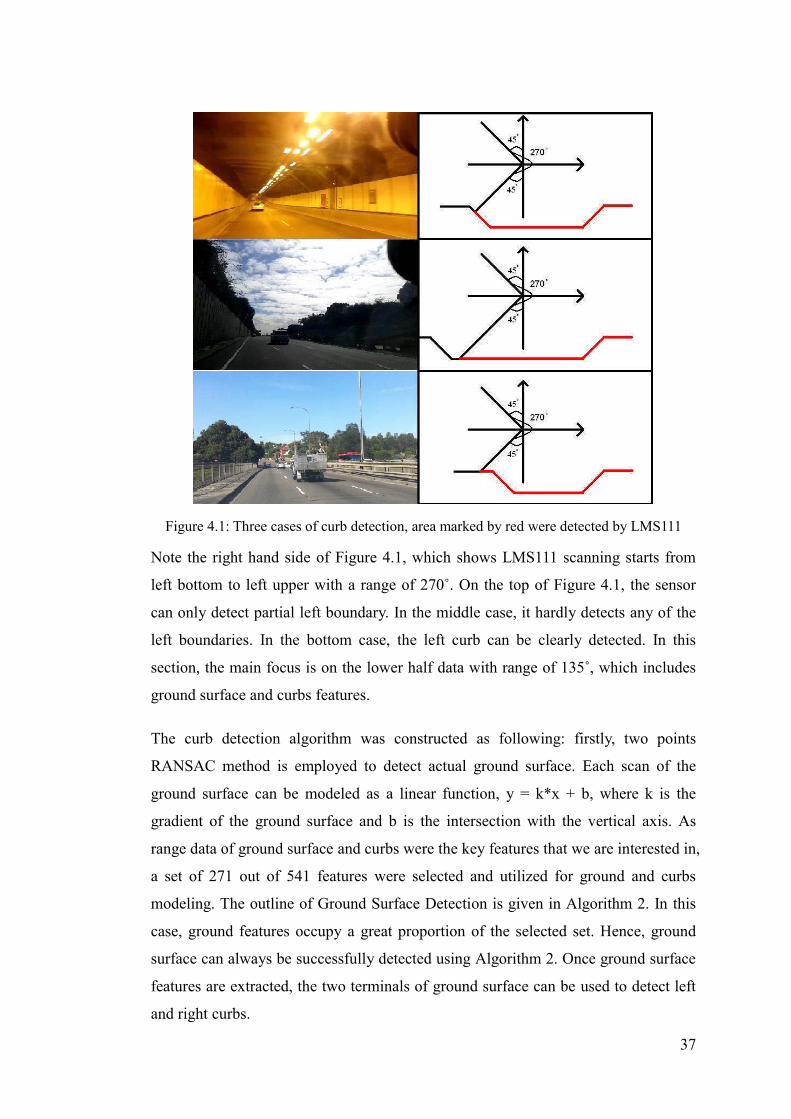
37
Figure 4.1: Three cases of curb detection, area marked by red were detected by LMS111
Note the right hand side of Figure 4.1, which shows LMS111 scanning starts from
left bottom to left upper with a range of 270˚. On the top of Figure 4.1, the sensor
can only detect partial left boundary. In the middle case, it hardly detects any of the
left boundaries. In the bottom case, the left curb can be clearly detected. In this
section, the main focus is on the lower half data with range of 135˚, which includes
ground surface and curbs features.
The curb detection algorithm was constructed as following: firstly, two points
RANSAC method is employed to detect actual ground surface. Each scan of the
ground surface can be modeled as a linear function, y = k*x + b, where k is the
gradient of the ground surface and b is the intersection with the vertical axis. As
range data of ground surface and curbs were the key features that we are interested in,
a set of 271 out of 541 features were selected and utilized for ground and curbs
modeling. The outline of Ground Surface Detection is given in Algorithm 2. In this
case, ground features occupy a great proportion of the selected set. Hence, ground
surface can always be successfully detected using Algorithm 2. Once ground surface
features are extracted, the two terminals of ground surface can be used to detect left
and right curbs.

38
ALGORITHM 2: GROUND SURFACE DETECTION
1. Initial: let A(271) be a set of N(541) feature correspondences
2. Repeat
2.1 Randomly select a sample of 2 points from A
2.2. Fit a linear model using 2 random points
2.3. Compute the distance of all other points to this model
2.4. Count the inliers (i.e. number of points whose distance from model <
threshold d )
2.5. Store inliers, inliers index and coefficients of model
2.6. Until maximum number of iterations reached
3. Choose the coefficients of model and inliers index with the most inliers as a best
solution of the problem
However, under some circumstances, such as experimental vehicle driven on a bi-
directional high way, would fail to detect ground surface and curb on a driveway. As
an example given in Figure 4.2, inliers index of ground surface are discontinued due
to interruption of a curb (width: 1.04 meter and height: 0.26 meter) in the middle. In
order to precisely detect ground surface and curb on a driveway, inliers index
containing discontinued sections have to be picked out and analyzed.
Continuous utilizing of the two points RANSAC method was used to identify the left
hand-side curb. As the left terminal of the ground surface has been explored, all
features on the left of left terminal can be formed as a new set and initialized in
Algorithm 2. A special case is shown in the middle of Figure 4.1; left terminal of
ground surface is the first data of entire set and the left curb is out of scan range.
Finally, applying a similar technique for left curb detection on right curb detection is
still effective. However, a set containing features from the right terminal of ground
surface to the end of the entire set is much more complicated to detect. Various
features, such as curbs, pavements, protective barriers and walls may be involved in
this set. Moreover, the right curb model usually does not have the most inliers to be
selected as a best solution. Hence, a few constraints are set to resolve the problem: 1)
Inliers index has to involve the right terminal of ground surface. 2) Inliers index has
to be consecutive. 3) Certain gradient changes between curb and ground.
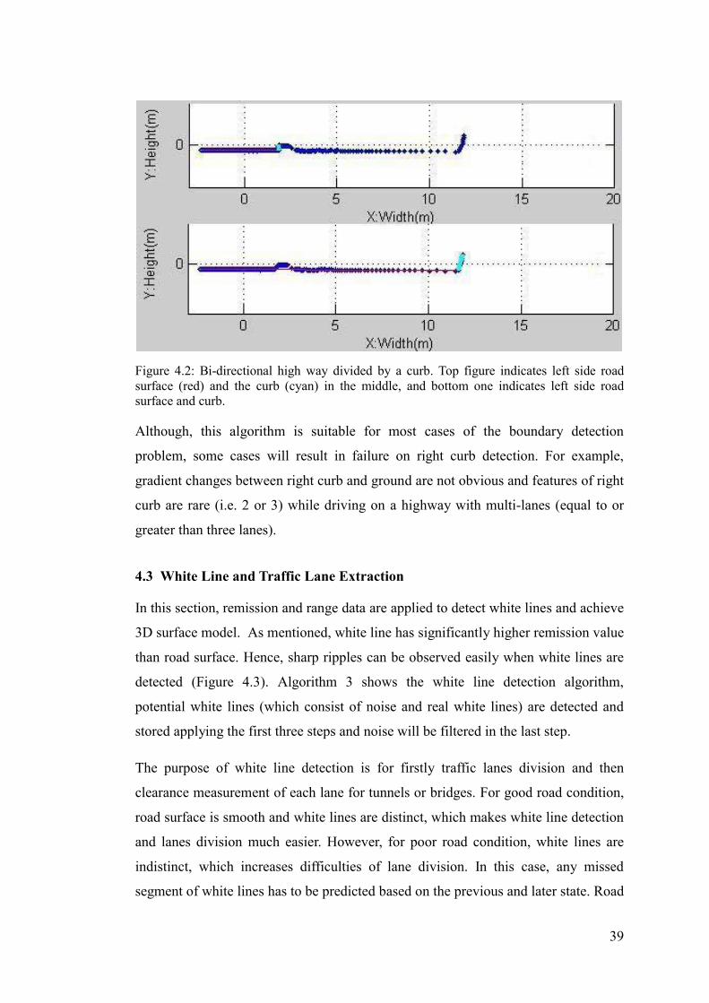
39
Figure 4.2: Bi-directional high way divided by a curb. Top figure indicates left side road surface (red) and the curb (cyan) in the middle, and bottom one indicates left side road surface and curb.
Although, this algorithm is suitable for most cases of the boundary detection
problem, some cases will result in failure on right curb detection. For example,
gradient changes between right curb and ground are not obvious and features of right
curb are rare (i.e. 2 or 3) while driving on a highway with multi-lanes (equal to or
greater than three lanes).
4.3 White Line and Traffic Lane Extraction
In this section, remission and range data are applied to detect white lines and achieve
3D surface model. As mentioned, white line has significantly higher remission value
than road surface. Hence, sharp ripples can be observed easily when white lines are
detected (Figure 4.3). Algorithm 3 shows the white line detection algorithm,
potential white lines (which consist of noise and real white lines) are detected and
stored applying the first three steps and noise will be filtered in the last step.
The purpose of white line detection is for firstly traffic lanes division and then
clearance measurement of each lane for tunnels or bridges. For good road condition,
road surface is smooth and white lines are distinct, which makes white line detection
and lanes division much easier. However, for poor road condition, white lines are
indistinct, which increases difficulties of lane division. In this case, any missed
segment of white lines has to be predicted based on the previous and later state. Road
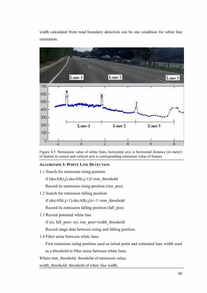
40
width calculated from road boundary detection can be one condition for white line
estimation.
Figure 4.3: Remission value of white lines, horizontal axis is horizontal distance (in meter) of feature to sensor and vertical axis is corresponding remission value of feature
ALGORITHM 3: WHITE LINE DETECTION
1.1 Search for remission rising position
if (decAll(i,j)-decAll(i,j-1))>rem_threshold
Record its remission rising position (rise_pos).
1.2 Search for remission falling position
if (decAll(i,j+1)-decAll(i,j))<-1×rem_threshold
Record its remission falling position (fall_pos).
1.3 Record potential white line
if x(i, fall_pos)- x(i, rise_pos)<width_threshold
Record range data between rising and falling position.
1.4 Filter noise between white lines
First remission rising position used as initial point and estimated lane width used
as a threshold to filter noise between white lines.
Where rem_threshold: threshold of remission value;
width_threshold: threshold of white line width.
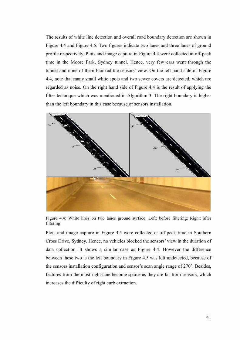
41
The results of white line detection and overall road boundary detection are shown in
Figure 4.4 and Figure 4.5. Two figures indicate two lanes and three lanes of ground
profile respectively. Plots and image capture in Figure 4.4 were collected at off-peak
time in the Moore Park, Sydney tunnel. Hence, very few cars went through the
tunnel and none of them blocked the sensors’ view. On the left hand side of Figure
4.4, note that many small white spots and two sewer covers are detected, which are
regarded as noise. On the right hand side of Figure 4.4 is the result of applying the
filter technique which was mentioned in Algorithm 3. The right boundary is higher
than the left boundary in this case because of sensors installation.
Figure 4.4: White lines on two lanes ground surface. Left: before filtering; Right: after filtering
Plots and image capture in Figure 4.5 were collected at off-peak time in Southern
Cross Drive, Sydney. Hence, no vehicles blocked the sensors’ view in the duration of
data collection. It shows a similar case as Figure 4.4. However the difference
between these two is the left boundary in Figure 4.5 was left undetected, because of
the sensors installation configuration and sensor’s scan angle range of 270˚. Besides,
features from the most right lane become sparse as they are far from sensors, which
increases the difficulty of right curb extraction.
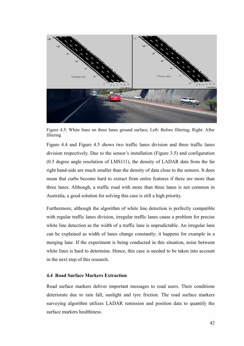
42
Figure 4.5: White lines on three lanes ground surface; Left: Before filtering; Right: After filtering
Figure 4.4 and Figure 4.5 shows two traffic lanes division and three traffic lanes
division respectively. Due to the sensor’s installation (Figure 3.5) and configuration
(0.5 degree angle resolution of LMS111), the density of LADAR data from the far
right hand-side are much smaller than the density of data close to the sensors. It does
mean that curbs become hard to extract from entire features if there are more than
three lanes. Although, a traffic road with more than three lanes is not common in
Australia, a good solution for solving this case is still a high priority.
Furthermore, although the algorithm of white line detection is perfectly compatible
with regular traffic lanes division, irregular traffic lanes cause a problem for precise
white line detection as the width of a traffic lane is unpredictable. An irregular lane
can be explained as width of lanes change constantly; it happens for example in a
merging lane. If the experiment is being conducted in this situation, noise between
white lines is hard to determine. Hence, this case is needed to be taken into account
in the next step of this research.
4.4 Road Surface Markers Extraction
Road surface markers deliver important messages to road users. Their conditions
deteriorate due to rain fall, sunlight and tyre friction. The road surface markers
surveying algorithm utilizes LADAR remission and position data to quantify the
surface markers healthiness.
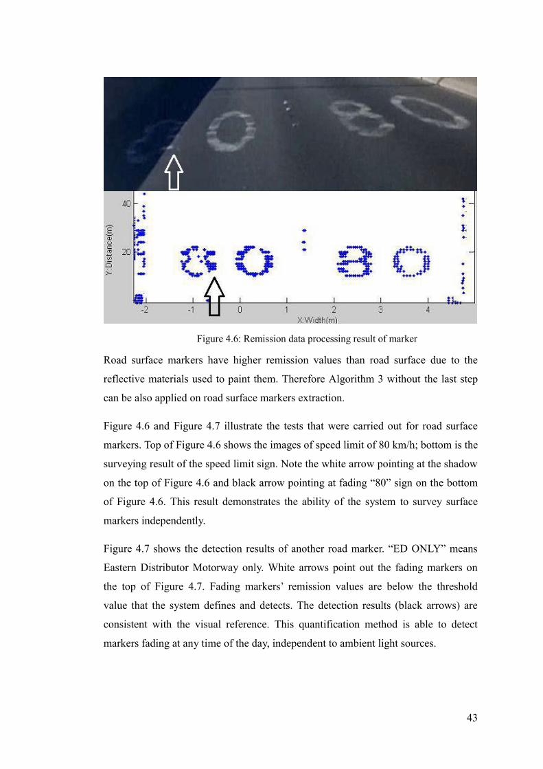
43
Figure 4.6: Remission data processing result of marker
Road surface markers have higher remission values than road surface due to the
reflective materials used to paint them. Therefore Algorithm 3 without the last step
can be also applied on road surface markers extraction.
Figure 4.6 and Figure 4.7 illustrate the tests that were carried out for road surface
markers. Top of Figure 4.6 shows the images of speed limit of 80 km/h; bottom is the
surveying result of the speed limit sign. Note the white arrow pointing at the shadow
on the top of Figure 4.6 and black arrow pointing at fading “80” sign on the bottom
of Figure 4.6. This result demonstrates the ability of the system to survey surface
markers independently.
Figure 4.7 shows the detection results of another road marker. “ED ONLY” means
Eastern Distributor Motorway only. White arrows point out the fading markers on
the top of Figure 4.7. Fading markers’ remission values are below the threshold
value that the system defines and detects. The detection results (black arrows) are
consistent with the visual reference. This quantification method is able to detect
markers fading at any time of the day, independent to ambient light sources.

44
Figure 4.7: Remission data processing result of marker
The proposed system also has a built-in function to monitor this road surface
markers’ abnormality. Once the system detected fading or unclear markers, a flash
warning signal was given on the data acquisition software along with an audible
warning. In the meantime, coordinates of the markers’ location are recorded and later
on will be matched with digital maps. This function is valuable for road authorities
to achieve efficient road monitoring and management.
4.5 Clearance Measurement for Tunnels and Bridges
Road assets clearance surveying is one of the most important aspects of road safety.
Over-height vehicles are often involved in bridge strike accidents with serious
consequences. The proposed system can resolve shortcomings of traditional manual
surveying, such as time consumption, causing traffic disruptions and being subject to
human errors.
LMS-111 scans both the overhead structure and the ground. Combined with the IMU
data, a cross-section plot is built perpendicular to the ground. Both LMS-111 and
LMS-400 data are plotted in the same coordinate system and interpolation of the data
is performed if necessary. LMS-111 data is processed for the cross-section build-up
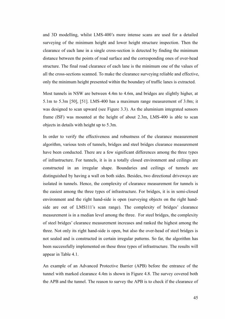
45
and 3D modelling, whilst LMS-400’s more intense scans are used for a detailed
surveying of the minimum height and lower height structure inspection. Then the
clearance of each lane in a single cross-section is detected by finding the minimum
distance between the points of road surface and the corresponding ones of over-head
structure. The final road clearance of each lane is the minimum one of the values of
all the cross-sections scanned. To make the clearance surveying reliable and effective,
only the minimum height presented within the boundary of traffic lanes is extracted.
Most tunnels in NSW are between 4.4m to 4.6m, and bridges are slightly higher, at
5.1m to 5.3m [50], [51]. LMS-400 has a maximum range measurement of 3.0m; it
was designed to scan upward (see Figure 3.3). As the aluminium integrated sensors
frame (ISF) was mounted at the height of about 2.3m, LMS-400 is able to scan
objects in details with height up to 5.3m.
In order to verify the effectiveness and robustness of the clearance measurement
algorithm, various tests of tunnels, bridges and steel bridges clearance measurement
have been conducted. There are a few significant differences among the three types
of infrastructure. For tunnels, it is in a totally closed environment and ceilings are
constructed in an irregular shape. Boundaries and ceilings of tunnels are
distinguished by having a wall on both sides. Besides, two directional driveways are
isolated in tunnels. Hence, the complexity of clearance measurement for tunnels is
the easiest among the three types of infrastructure. For bridges, it is in semi-closed
environment and the right hand-side is open (surveying objects on the right hand-
side are out of LMS111’s scan range). The complexity of bridges’ clearance
measurement is in a median level among the three. For steel bridges, the complexity
of steel bridges’ clearance measurement increases and ranked the highest among the
three. Not only its right hand-side is open, but also the over-head of steel bridges is
not sealed and is constructed in certain irregular patterns. So far, the algorithm has
been successfully implemented on these three types of infrastructure. The results will
appear in Table 4.1.
An example of an Advanced Protective Barrier (APB) before the entrance of the
tunnel with marked clearance 4.4m is shown in Figure 4.8. The survey covered both
the APB and the tunnel. The reason to survey the APB is to check if the clearance of
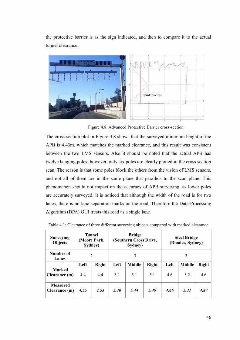
46
the protective barrier is as the sign indicated, and then to compare it to the actual
tunnel clearance.
Figure 4.8: Advanced Protective Barrier cross-section
The cross-section plot in Figure 4.8 shows that the surveyed minimum height of the
APB is 4.43m, which matches the marked clearance, and this result was consistent
between the two LMS sensors. Also it should be noted that the actual APB has
twelve hanging poles; however, only six poles are clearly plotted in the cross section
scan. The reason is that some poles block the others from the vision of LMS sensors,
and not all of them are in the same plane that parallels to the scan plane. This
phenomenon should not impact on the accuracy of APB surveying, as lower poles
are accurately surveyed. It is noticed that although the width of the road is for two
lanes, there is no lane separation marks on the road. Therefore the Data Processing
Algorithm (DPA) GUI treats this road as a single lane.
Table 4.1: Clearance of three different surveying objects compared with marked clearance
Surveying Objects
Tunnel (Moore Park,
Sydney)
Bridge (Southern Cross Drive,
Sydney)
Steel Bridge (Rhodes, Sydney)
Number of Lanes 2 3 3
Marked
Clearance (m)
Left Right Left Middle Right Left Middle Right
4.4 4.4 5.1 5.1 5.1 4.6 5.2 4.6
Measured Clearance (m)
4.55 4.53 5.30 5.44 5.49 4.66 5.31 4.87

47
The tunnel detailed surveying result is presented in Figure 4.10 and clearance results
are summarized in Table 4.1. According to the IMU measurements and wheel
odometry, the tunnel is descending and then ascending. The measured length of the
tunnel is 465.23m. There are two lanes in the tunnel, and two individual clearances
are extracted from the surveying data. The dotted white line in Figure 4.10 represents
the actual white line in the middle of the road that separates the two traffic lanes.
Two cross-section plots in the DPA GUI present the two sections in which minimum
clearance is measured for each lane. Figure 4.10shows the details of cross section
plot at the clearance point of the right lane on the right, and a photo of the tunnel on
the top left. A red and blue line in the figure points out the bulge that causes the
minimum clearance and its relative position on the ground.
The surveying results show that the minimum clearance of the left lane is 4.55m. It is
located at the point 19.93m from the entrance and 1.81m from the road left border.
The minimum clearance of the right lane is 4.53m, and is located at the point 82.60m
from the entrance and 6.23m from the road left border.
The surveying results show that the marked clearance of APB with 4.4m is
consistent with the surveyed result. The tunnel’s clearance is 4.55m on the left lane
and 4.53m on the right lane. Although the surveyed clearance of the tunnel is slightly
higher than the sign marked 4.4m, it is safe for vehicles under 4.4m to pass.
Several bridges were surveyed during the test. A pedestrian bridge over the Southern
Cross Drive is taken as an example. The measured clearance of the left lane is 5.30m,
at the point of 7.99m from the beginning of the bridge and 0.88m from the left
border. For the middle lane, the clearance is 5.44m, at 7.99m from the beginning and
3.94m from the left border. The clearance of the right lane is 5.49m, at 7.64m from
the beginning and 7.04m from the left border.
Note that in the clearance cross-section plot of the pedestrian bridge over two
directional drive ways, only half of the bridge can be plotted as measurable by the
LMS111 sensor. This is due to the fact that the LMS111 sensor could only pick up a
10m range with 13% remission value [46]

48
Comparing the measured clearance (the testing results) and marked clearance
(clearance marked on signs before entering into tunnels or bridges) for three
surveying objects, the measured clearance of the tunnel and the steel bridge is in
better agreement than for that of the bridge. The reason for this disparity could be
that surveyors take clearance measurement beyond the white line into account. As the
bridge has an arc shape, the clearance within the white lines would be definitely
higher than the clearance beyond the white lines. More importantly, it is necessary to
keep the actual road clearance higher than it is indicated, so as to ensure vehicles up
to the height-limit drive through safely.
In the current stage, reasonable clearance measurement results of three types of
surveying objects have been made. However, the actual accuracy of clearance
measurement results is still unknown. Marked clearance sometimes is not identical to
the actual clearance due to the deformation of infrastructures and other issues. Due to
time constrains, I have not gotten in touch with the RTA at this stage. Hence, the next
step of this part of the research is to contact the RTA for verifying the actual
accuracy of measured clearance results. Finally the current algorithm of clearance
measurement is capable of working under the particular situation that no vehicle is
blocking the right hand side of the sensors on the right-hand side of sensors. Any
area blocked by other vehicles is hard to predict. Hence, another potential
improvement on this algorithm is to find a possible way of predicting data in a
blocked area with high accuracy. The significance of this improvement is that it will
make the proposed system work on both traffic peak time and off-peak time.
4.6 3D Model and GUI Construction
The purpose of constructing a 3D model is to provide a genuine view of road assets
and the reason for constructing a GUI is to integrate all functions into one interface
to finally present comprehensive surveying results. In the following, the way to
construct a 3D model and a GUI will be presented in detail.
After combining the road boundary detection and white line detection algorithm, the
basic road profile is now available. Roll-pitch-yaw motion data from IMU and
instant speed data from odometer, which applied on previous road profiling, are used
to generate 3D road surface model.

49
A rotation matrix is produced based on roll-pitch-yaw information, which gives the
transformation of scan data [52]:
(4.1)
Where: is yaw; is pitch; is roll.
Each scan data generated by LMS111 can be transferred into a global coordinate
system. Figure 4.9 shows the 3D road surface model in a tunnel. An enlarged short
section of the tunnel is also presented in Figure 4.4.
However, using IMU alone to obtain attitude would cause inaccurate trajectory of the
road surface, because the error of IMU will be accumulated over time. To minimize
the error issue, a visual odometry method will be introduced into the system in the
next section.
Road 3D models include name, data of surveying, clearance of traffic lanes and
conditions of road assets. Road 3D modelling helps the Roads and Traffic Authority
to construct a database and, integrated with Geographic Information System (GIS),
to monitor and manage road assets.
The lowest clearance point of each lane is indicated in the 3D model and presented
in the GUI. The 3D model delivers the most intuitional profile of surveyed objects,
and includes lines on the road surface and the location of clearance points. As an
example of the 3D model is shown in Figure 4.9, image frames are extracted from
camera and displaced on the top left part of the GUI. The purpose of embedding
video frames to GUI is firstly to provide video reference for features verification.
Secondly, video frames can be used for gaining PVA information. Specially, in GPS
denied environments such as tunnels, visual odometry is a very good solution,
substituting for the absence of GPS information. In chapter 5, visual odometry of
gaining PVA will be introduced.
)(R)(R)(R),,(R xyz
coscossincossinsincoscossinsincoscossinsinsincossinsinsincossincoscossinsinsincoscoscos

50
Figure 4.9: 3D Road Surface model of a tunnel
The bottom section of the GUI displays an overview map of the air view and side-
looking view respectively while a zoom-in air view is processed on the left bottom
part of the GUI. The reason for arranging a zoom-in air view is to make sure road
surface condition can be clearly observed. The position of current minimum height
of each lane is indicated and marked in different colours in both air view plotting and
side view plotting. It presents real-time spatial view of clearance, which offers
greater assistance for surveyors to get clearance information in minimum time.
In the middle top of the GUI, cross section of clearance measurement is plotted.
Number of lanes is worked out automatically in the data processing algorithm. At the
same time, the exact same number of cross section windows is presented for
displaying clearance measurement results. Any latest minimum height result of
surveying object is updated automatically in the text editing area where is located
under the cross section window. In addition, clearance positioning information is
also calculated and displayed in the text area.

51
A few buttons on the most right hand-side are developed for operation convenience.
All well-prepared data (LADARs data, video stream and navigation data) are able to
be loaded once using Load files button. Any faulty data and format will be alarmed
and prohibited. On the right hand-side of load files button, a short text content is
proposed to indicate the loading state whether it is complete or incomplete, and then
to prevent any improper operation during the incomplete loading state. After data
loading, types of surveying objects (such as tunnels and high ways) and number of
lanes is determined automatically according to their characteristics. A radio button is
embedded in the GUI, which is an optional record button for converting GUI frames
into a movie. The advantage is that it saves time for the next time review. However, a
disadvantage is still worth noting, which is the time consumed in data processing.
The PLAY VIDEO button is designed only for video stream displaying. Video
frames in the GUI are consistent with LADADs’ data by matching their clock. The
PLAY/PAUSE button is implemented for presenting road asset animation and results.
The function of the REST button is to clear all input data information and existing
GUI frames after the animation is paused. In a word, the proposed GUI is acting as a
data media player, which is designed with the particular specification and
requirement developed in this study.
Figure 4.10: Road 3D modelling in GUI, Eastern Distributor Motorway tunnel, Sydney

52
A GUI in Figure 4.10 demonstrates a road asset result in the Eastern Distributor
Motorway tunnel, Sydney, which integrates functions mentioned above. The
proposed system is designed for on-line processing. It is able to deliver direct
profiles and comprehensive road asset results immediately while driving for
experimental road tests.
Although the proposed GUI has been developed in a user-friendly interface, there is
still some room for further improvement in the future, such as adding a play time line
in the GUI. Users can watch any animation moment which they are interested in by
selecting the play time.
4.7 Road Roughness Measurement
In the road roughness measurement section, the condition of the road surface is a
major concern. In order to obtain more detailed road surface roughness results, the
LMS 400 with higher frequency was rotated 180 degree to look downwards and the
ISF was modified based on the first design.
Road roughness measurement over longitudinal road profiles is used to determine
road surface quality. Road Roughness Measurement can be also expressed in terms
of index like the International Roughness Index (IRI), which quantifies the
tolerability of road roughness at different speeds [53].
The IRI is a cumulative measurement of changes in elevation or roughness [54]. It is
expressed in dimensionless units of mm/km or in/mi. Appendix A and Appendix B
shows roughness scales from ASTM E1926-08 that correlates IRI (mm/km) values
with estimations of ride quality.
The IRI value is calculated based on data from LADAR sensors. Road surface
profiling using the proposed system to generate a dense point cloud in three
dimensional spatial coordinates (Figure 4.11) delivers accurate raw data for
roughness measurement. The scope of this section is the implementation of the IRI
and its incorporation into the existing mobile surveying system.
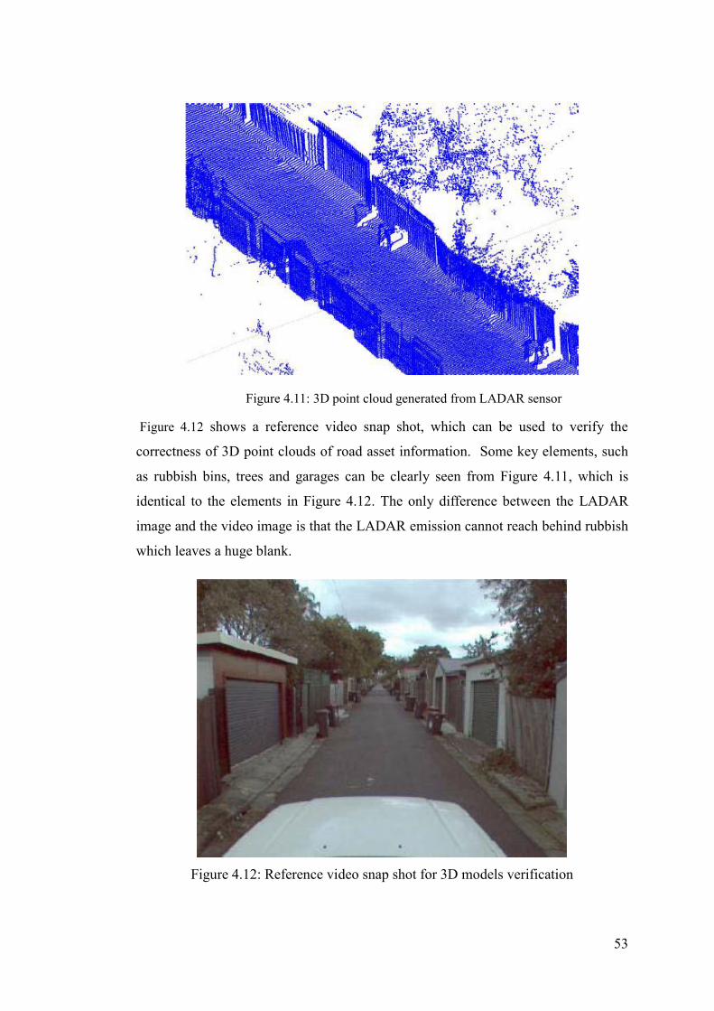
53
Figure 4.11: 3D point cloud generated from LADAR sensor
Figure 4.12 shows a reference video snap shot, which can be used to verify the
correctness of 3D point clouds of road asset information. Some key elements, such
as rubbish bins, trees and garages can be clearly seen from Figure 4.11, which is
identical to the elements in Figure 4.12. The only difference between the LADAR
image and the video image is that the LADAR emission cannot reach behind rubbish
which leaves a huge blank.
Figure 4.12: Reference video snap shot for 3D models verification

54
While the RTA may require longitudinal profiles generated from wheel paths
perfectly centred within road lanes (Figure 4.13), more realistic roughness
measurements may be additionally calculated using arbitrary wheel path lines
through corners to better simulate realistic driving behaviour using bend radius
and/or camber information (Figure 4.14).
Figure 4.13: Longitudinal profile lines required by the RTA
Figure 4.14: Different wheel paths through the same road curve give different profiles
The sample FORTRAN program defined in ASTM E1926-08 has been translated
into Matlab code for ease of code interfacing and integration. The parameters of this
algorithm are based on ‘golden car’, which takes regard of a reference point for
calibration [28, 29]. Detailed Matlab code can be seen in Appendix C. The
effectiveness of translated Matlab code has been successfully verified using the
sample profile data provided.

55
The current roughness profile algorithm focuses on longitudinal profile data at the
vehicle wheels position. Extracting any number of profile lines from a 3D dense
point cloud can be an easy task and the algorithm can be varied without changing
any structure. The multiple profile lines may be developed as necessary (Figure 4.15).
Figure 4.15: Multiple profile lines for roughness measurement are extracted as necessary
Tests have been conducted on in various road surfaces, such as asphalt, concrete and
gravel. The asphalt surveying tests were conducted around a residential loop around
Jellicoe Park, Pagewood NSW with a perimeter of about 1000m (Figure 4.16). The
testing vehicle aimed to maintain speeds of 20, 30, 40 and 50 km/h.
Figure 4.16: Site of asphalt survey test, Jellicoe Park, Pagewood NSW

56
The concrete surveying tests were conducted around a small park lot at Heffron Park,
Maroubra NSW (Figure 4.17) with a perimeter of about 300m. The testing vehicle
aimed to maintain speeds of 20, 30, and 40 km/h.
Figure 4.17: Site of concrete survey test, Heffron Park, Maroubra NSW
The gravel surveying tests were conducted along a four wheel drive access road
along Warumbul Road, Bundeena NSW with a length of about 1.4km (Figure 4.18).
The testing vehicle aimed to maintain speeds of 10, 20 and 30km/h.
Figure 4.18: Site of gravel survey test, Warumbul Road, Bundeena NSW
By only looking at roughness of asphalt, concrete and gravel from images showing
in Figure 4.16 to Figure 4.18, the first conducted test on asphalt road surface has the
best road condition, while road condition of concrete surface ranked in the middle
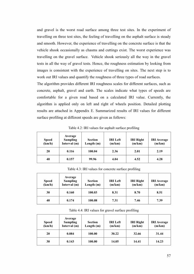
57
and gravel is the worst road surface among three test sites. In the experiment of
travelling on three test sites, the feeling of travelling on the asphalt surface is steady
and smooth. However, the experience of travelling on the concrete surface is that the
vehicle shook occasionally as chasms and cuttings exist. The worst experience was
travelling on the gravel surface. Vehicle shook seriously all the way in the gravel
tests in all the way of gravel tests. Hence, the roughness estimation by looking from
images is consistent with the experience of travelling on sites. The next step is to
work out IRI values and quantify the roughness of three types of road surfaces.
The algorithm provides different IRI roughness scales for different surfaces, such as
concrete, asphalt, gravel and earth. The scales indicate what types of speeds are
comfortable for a given road based on a calculated IRI value. Currently, the
algorithm is applied only on left and right of wheels position. Detailed plotting
results are attached in Appendix E. Summarized results of IRI values for different
surface profiling at different speeds are given as follows:
Table 4.2: IRI values for asphalt surface profiling
Speed (km/h)
Average Sampling
Interval (m) Section
Length (m) IRI Left (m/km)
IRI Right (m/km)
IRI Average (m/km)
20 0.116 100.04 2.36 2.01 2.19
40 0.157 99.96 4.04 4.52 4.28
Table 4.3: IRI values for concrete surface profiling
Speed (km/h)
Average Sampling
Interval (m) Section
Length (m) IRI Left (m/km)
IRI Right (m/km)
IRI Average (m/km)
30 0.160 100.03 8.31 8.70 8.51
40 0.174 100.08 7.31 7.46 7.39
Table 4.4: IRI values for gravel surface profiling
Speed (km/h)
Average Sampling
Interval (m) Section
Length (m) IRI Left (m/km)
IRI Right (m/km)
IRI Average (m/km)
20 0.084 100.00 30.22 32.66 31.44
30 0.143 100.00 14.05 14.41 14.23

58
In Table 4.2, quite small average IRI values are calculated at different speeds which
means people can have a comfortable ride up to more than 90 km/h (Appendix A) on
this sampling asphalt surface. By contrast, average IRI values are extremely large in
Table 4.4 as people have a comfortable ride up to a very limited speed (Appendix B)
on this sampling gravel surface. In Table 4.3, average IRI values on concrete
sampling surface are approximately two times larger than the average IRI values on
asphalt surface. People would ride comfortably up to 50-60 km/h in this situation.
The reason which causes this result is that there are many obvious cuttings between
single concrete sections.
4.8 Summary
This chapter presented a novel method for automatic road clearance surveying, road
surface profiling, 3D structure modelling, road boundary detection and road
roughness measurement. It gives road maintainers the power to survey road
clearance without a hazard to labour and disrupting traffic. With sensors fusion
technologies and data processing algorithms, 3D models of bridge and tunnel marked
with the lowest point of each lane are constructed. Even under ambient interference,
surveying data still can be processed to obtain a road clearance result. Moreover, the
proposed system is adapted with modular design; new components can be added into
the system easily.
The road assets’ clearance is acquired by combining LADAR range and INS attitude
data. The road surfaces conditions are detected by examining the LADAR range and
INS acceleration data. Healthiness of road surface markers is determined by
processing images, LADAR remission and INS data, while road boundary detection
is completed by advanced filtering algorithm. Road assets 3D model is constructed
in the GUI for visualization of surveying results and management of database.
Longitudinal profiles were generated from dense point cloud 3D model data by
simply extracting points falling beneath the wheel tracks, and averaging their relative
heights to reduce to a single left and right wheel profile value for each scan line.
Results of real environment road tests under different conditions have demonstrated
the capability and robustness of a prototype surveying system.

59
There is much potential that surveying system could be improved. A GPS, IMU and
Odometer integrated navigation system will provide much better position and
attitude information to improve the system performance. Cooperation with roads and
traffic authority is expected to test the system for robustness and feasibility
evaluation.
60
CHAPTER 5 VISUAL ODOMETRY
OPTIMIZATION
5.1 Introduction During the past few driving tests in the urban area of Sydney, GPS signal became
unreliable when the experimental vehicle was driven in some closed areas, such as
tunnels. Hence, it was decided to introduce visual odometry as a backup method for
obtaining continuous and accurate PVA information into the proposed system. Visual
odometry is composed by feature detection, feature matching, robust estimation of
fundamental matrix and camera pose optimization.
SURF [55] method has been utilized for feature detection and matching. RANSAC
has been used for about thirty years as the benchmark method for model fitting in the
presence of outliers, as well as an estimation method of fundamental matrix.
It estimates a model that fits the provided data, while simultaneously classifying the
data into inliers (samples consistent with the relation) and outliers (samples not
consistent with the relation). It is a simple yet powerful technique that can estimate a
model using data contaminated by a large fraction of outliers. RANSAC can be
briefly summarized as a hypothesize-and-verify framework: a minimal subset of
samples for model fitting is randomly selected from the entire dataset. The subset is
then used to fit model hypotheses which are evaluated on the entire dataset by
computing the distance of all other samples to this model and constructing an inliers’
set with a threshold. This hypothesize-and-verify loop is repeated until the
probability of finding a model with better consensus than the current best model falls
below a predefined threshold.
The principle steps of RANSAC can be summarized as: 1) randomly select a set of
samples from all the samples; 2) fit a model hypotheses with the selected set of
samples; 3) compute the distance of all other points to this model; 4) construct the
inliers set with a distance threshold, compare its inliers count to the previous highest
one and store the results. Steps 1 to 4 are repeated until a pre-set threshold of
iterations is reached. The set with maximum number of inliers is chosen, all these
inliers are used for model parameter estimation [32].

61
For generality and simplicity, RANSAC is based on a set of assumptions, which are
not true in many real situations. This leaves large room for improvement. In this
section, as part of my contributions in this research, new algorithm named PURSAC
(PURposive Sample Consensus) for model fitting is introduced, which purposely
selects sample sets according to the sensitivity analysis of a model against sampling
noise, and other information that can be used for purposive selection. PURSAC is a
strategy for sample sets selection, which can be combined with any model fitting
algorithms that use random sample sets selection. Comparing to RANSAC and
MLESAC (maximum likelihood estimation sample consensus), PURSAC can detect
more inliers with much fewer number of iterations and in turn can improve both the
efficiency and reliability of model fitting. This is very important for applications
where speed and precision is critical, such as visual odometry (VO). With analysis
about a model’s sensitivity against sampling noise and the pattern of samples’
validity, PURSAC is designed to efficiently handle both sampling noise and outliers
for model fitting.
Experimental results with publically available data demonstrate that PURSAC can be
easily combined with existing model fitting algorithms, and detect more inliers with
a lesser number of iterations. In visual odometry this in turn can improve the
accuracy and robustness of fundamental matrix estimation, resulting in a more
precise and efficient visual odometry result.
5.2 Justification of PURSAC in Visual Odometry
In GPS denied environment, visual odometry is utilised as a backup method for
obtaining continuous and accurate PVA. The proposed method, PURSAC, is
developed based on RANSAC which has been used for about thirty years as a
benchmark method for model fitting in the presence of outliers. As one component in
Visual Odometry, it plays the significant role of acquiring PVA information. Hence, a
robust estimation method delivers an accurate PVA result which is beneficial to the
proposed surveying project. This section presents the justification of the purposed
estimation method, PURSAC.
The RANSAC scheme is a fundamentally stochastic algorithm without deterministic
guarantees of finding the global maximum of the likelihood. It finds the best

62
hypothesis from some particular set of hypotheses, which have been generated
randomly in the first place.
A success rate p is defined in RANSAC for a certain level of confidence of finding a
consensus set, which is a function of the number of iterations to be conducted N,
sample outlier rate ε and number of samples in a set s [31]. The success rate here in
(2.1) simply means that a set of samples selected by RANSAC are all from inliers.
As observed, RANSAC is a probabilistic method and is nondeterministic in that it
exhibits different solutions on different runs. Its model fitting performance is
unsatisfactory for many applications, such as VO. In principle, the accuracy and
efficiency of a model fitting algorithm using random sampling can be improved if
the random sample set selection can be avoided, which is what PURSAC will
attempt to achieve.
Reconsideration is now given to the line-fitting example in the original RANSAC
paper [32]. As shown in Figure 5.1, two types of measurement errors (noise and
outlier) exist in the sample points. By randomly selecting a set of samples (two
points for line fitting) from all the samples, RANSAC can eliminate most if not all
the outliers after a certain number of iterations. At the same time, however, it also
likely rejects some inliers and so reduces the accuracy of model fitting. Due to the
measurement noise, model hypotheses selected by RANSAC with a limited number
of iterations usually cannot fit a model well, as illustrated in Figure 5.1. It is safe to
conclude that RANSAC is only effective in removing measurement outliers but is
inadequate for handling measurement noise.
Figure 5.1: Line fitting results by RANSAC (Line 1), PURSAC (Line 2) and least square (Line 3).
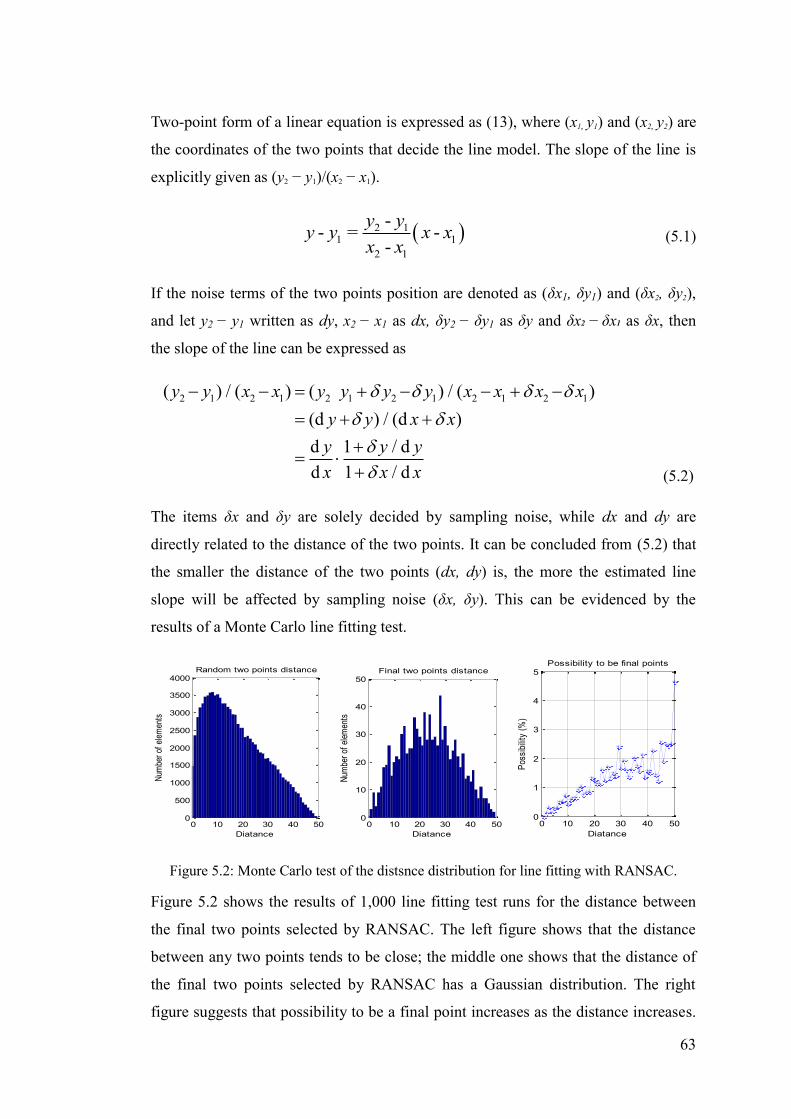
63
Two-point form of a linear equation is expressed as (13), where (x1, y1) and (x2, y2) are
the coordinates of the two points that decide the line model. The slope of the line is
explicitly given as (y2 − y1)/(x2 − x1).
2 11 1
2 1
-- = --
y yy y x xx x (5.1)
If the noise terms of the two points position are denoted as (δx1, δy1) and (δx2, δy2),
and let y2 − y1 written as dy, x2 − x1 as dx, δy2 − δy1 as δy and δx2 − δx1 as δx, then
the slope of the line can be expressed as
2 1 2 1 2 1 2 1 2 1 2 1 / / ( ) /
/
( ) ( ) ( )(d ) (d )d 1 dd d/1
y y x x y y y y x x x xy y x xy y yx x x
(5.2)
The items δx and δy are solely decided by sampling noise, while dx and dy are
directly related to the distance of the two points. It can be concluded from (5.2) that
the smaller the distance of the two points (dx, dy) is, the more the estimated line
slope will be affected by sampling noise (δx, δy). This can be evidenced by the
results of a Monte Carlo line fitting test.
Figure 5.2: Monte Carlo test of the distsnce distribution for line fitting with RANSAC.
Figure 5.2 shows the results of 1,000 line fitting test runs for the distance between
the final two points selected by RANSAC. The left figure shows that the distance
between any two points tends to be close; the middle one shows that the distance of
the final two points selected by RANSAC has a Gaussian distribution. The right
figure suggests that possibility to be a final point increases as the distance increases.
0 10 20 30 40 500
500
1000
1500
2000
2500
3000
3500
4000Random two points distance
Diatance
Num
ber o
f elem
ents
0 10 20 30 40 500
10
20
30
40
50Final two points distance
Diatance
Numb
er of
eleme
nts
0 10 20 30 40 500
1
2
3
4
5Possibility to be final points
Diatance
Poss
ibility
(%)

64
This indicates that the distance between the two points for the best consensus set
tends to be large, so as to dilute the effects of sampling noise for model fitting.
Consequently the two sample points should be selected a large distance apart.
The sample points themselves do not have any information available about their
validity for line fitting. It is impossible to rank or score the points without any prior
knowledge about them. However, it is known that for a line model some of the
points are inliers and other are outliers, and their validity will be assessed during the
process of classifying them. This validity information can be used to purposively
select points afterward that have a higher possibility to be inliers so as to speed up
the model fitting process.
Similar to locally optimized RANSAC [60], by observing that a good model tends to
find a significant fraction of the inliers, an inner iteration is executed. After a very
small number of iterations k, the set of inliers to the current best model is generated
with RANSAC or MLESAC. Then the next sample subset is selected only from the
current inliers and verified against the entire dataset. As the sampling is running on
current inliers dataset, there is no need for the size of sample subset to be minimal.
On the contrary, to mitigate sampling noise, the size should be selected to minimize
the error of the model parameter estimation.
This local optimization technique has the effect of improving the consensus score
more rapidly and causes the iteration termination criterion (N in(1)) to be met earlier
by selecting samples from current inliers set, which has a lower outlier rate than the
entire dataset has. In addition it can also provide more robust and precise model
fitting by minimizing the error of model estimation with proper sample size.
Considering the two observations about samples geometry and validity for the line
fitting tests, PURSAC is designed to purposely select two points far apart, instead of
random selection. The first point is randomly selected; then the distances from it to
all the other points are calculated. The second point is selected according to the
statistical distribution shown in Figure 5.2. Inner iteration is then applied by
selecting samples only from the current inliers until reaching iteration termination
criterion (1). Finally local optimization is implemented and all the inliers are used
iteratively to compute the final model parameters.
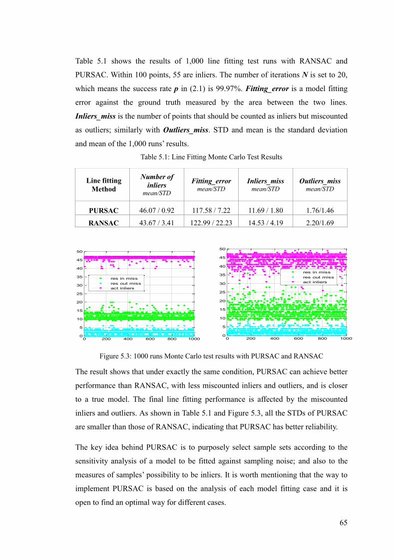
65
Table 5.1 shows the results of 1,000 line fitting test runs with RANSAC and
PURSAC. Within 100 points, 55 are inliers. The number of iterations N is set to 20,
which means the success rate p in (2.1) is 99.97%. Fitting_error is a model fitting
error against the ground truth measured by the area between the two lines.
Inliers_miss is the number of points that should be counted as inliers but miscounted
as outliers; similarly with Outliers_miss. STD and mean is the standard deviation
and mean of the 1,000 runs’ results. Table 5.1: Line Fitting Monte Carlo Test Results
Figure 5.3: 1000 runs Monte Carlo test results with PURSAC and RANSAC
The result shows that under exactly the same condition, PURSAC can achieve better
performance than RANSAC, with less miscounted inliers and outliers, and is closer
to a true model. The final line fitting performance is affected by the miscounted
inliers and outliers. As shown in Table 5.1 and Figure 5.3, all the STDs of PURSAC
are smaller than those of RANSAC, indicating that PURSAC has better reliability.
The key idea behind PURSAC is to purposely select sample sets according to the
sensitivity analysis of a model to be fitted against sampling noise; and also to the
measures of samples’ possibility to be inliers. It is worth mentioning that the way to
implement PURSAC is based on the analysis of each model fitting case and it is
open to find an optimal way for different cases.
0 200 400 600 800 10000
5
10
15
20
25
30
35
40
45
50
res in missres out missact inliers
0 200 400 600 800 10000
5
10
15
20
25
30
35
40
45
50
res in missres out missact inliers
Line fitting Method
Number of inliers
mean/STD Fitting_error
mean/STD Inliers_miss
mean/STD Outliers_miss
mean/STD
PURSAC 46.07 / 0.92 117.58 / 7.22 11.69 / 1.80 1.76/1.46
RANSAC 43.67 / 3.41 122.99 / 22.23 14.53 / 4.19 2.20/1.69
66
5.3 Outline of applying PURSAC to Visual Odometry RANSAC and MLESAC has been widely used in computer vision, particularly in
the areas of recovering epipolar geometry and 3D motion estimation, such as image
registration, structure from motion and feature based VO. The motion of an agent
(vehicle, human or robot etc.) can be estimated by incrementally estimating the pose
of the agent through examination of the movement induced on the images of its on
board camera(s) [31]. Feature based VO uses salient and repeatable features
extracted and is matched across the captured images. No matter which algorithm is
used, the matched features are usually contaminated by outliers (wrong data
associations). How to efficiently remove the outliers is the most delicate task in VO
and still has large room for improvement.
This section introduces how to apply PURSAC to VO. The relations of features
matching scores to their possibility to be outliers and to their location accuracy in
images are investigated first. Then the sensitivity analysis of the egomotion model
against samples noise is conducted. Based on these analyses PURSAC is elaborated
aiming to design a purposive sample set selection procedure for the fundamental
matrix estimation, and to improve the results of outlier removal and model fitting
and in turn the VO performance.
5.3.1 Feature Measurement Analysis First let us analyse the relation between the feature matching score and the features’
possibility to be outlier. This has been done previously for SIFT [56] and some other
descriptors [61]. In all experiments, regardless of the similarity function used, the
fraction of inliers decreased almost monotonically as a function of the number of
tentative correspondences [39]. This is verified by the test results of this study for
169 pairs of images using SURF features [55]. Figure 5.4 shows that the matched
features with lower ranking have a higher likelihood of being outliers.
Another test was conducted to evaluate robustness and accuracy of SIFT and SURF
features’ location and it’s relation to the feature matching scores. Figure 5.5 is a test
result with SIFT features. The X axis is the feature location accuracy in pixel. Y axis
is the matching score from SIFT feature matching, which measures the 'confidence'
of the feature matching being correct. It shows as the confidence increases, so does

67
feature location accuracy (to an extent). This location uncertainty can be treated as
measurement noise, which has a relation with feature matching score. This result will
be used in the design of the rule for PURSAC’s purposive sample set selection.
Figure 5.4: Outliers and score ranking test
Figure 5.5: Features’ location accuracy and matching score correspondence.
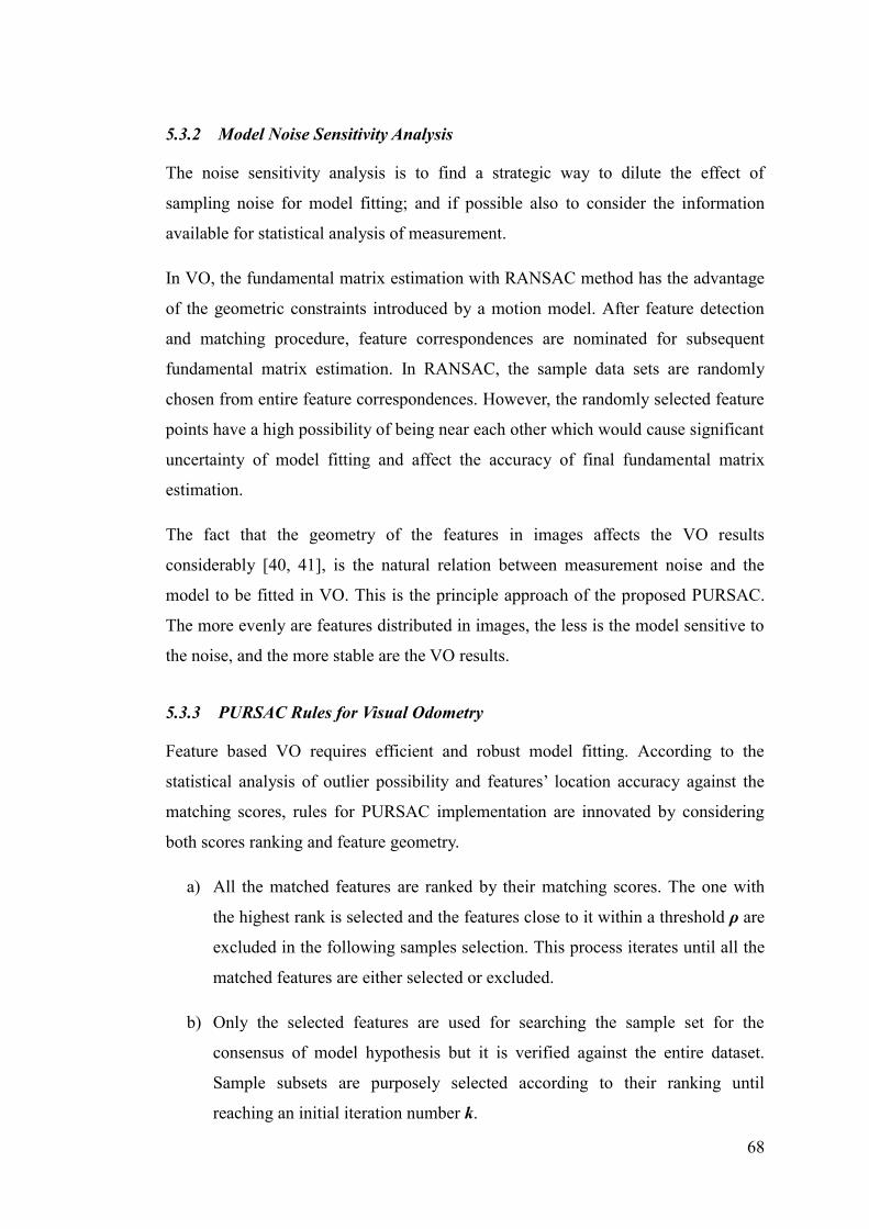
68
5.3.2 Model Noise Sensitivity Analysis
The noise sensitivity analysis is to find a strategic way to dilute the effect of
sampling noise for model fitting; and if possible also to consider the information
available for statistical analysis of measurement.
In VO, the fundamental matrix estimation with RANSAC method has the advantage
of the geometric constraints introduced by a motion model. After feature detection
and matching procedure, feature correspondences are nominated for subsequent
fundamental matrix estimation. In RANSAC, the sample data sets are randomly
chosen from entire feature correspondences. However, the randomly selected feature
points have a high possibility of being near each other which would cause significant
uncertainty of model fitting and affect the accuracy of final fundamental matrix
estimation.
The fact that the geometry of the features in images affects the VO results
considerably [40, 41], is the natural relation between measurement noise and the
model to be fitted in VO. This is the principle approach of the proposed PURSAC.
The more evenly are features distributed in images, the less is the model sensitive to
the noise, and the more stable are the VO results.
5.3.3 PURSAC Rules for Visual Odometry
Feature based VO requires efficient and robust model fitting. According to the
statistical analysis of outlier possibility and features’ location accuracy against the
matching scores, rules for PURSAC implementation are innovated by considering
both scores ranking and feature geometry.
a) All the matched features are ranked by their matching scores. The one with
the highest rank is selected and the features close to it within a threshold ρ are
excluded in the following samples selection. This process iterates until all the
matched features are either selected or excluded.
b) Only the selected features are used for searching the sample set for the
consensus of model hypothesis but it is verified against the entire dataset.
Sample subsets are purposely selected according to their ranking until
reaching an initial iteration number k.

69
c) In the same way as the line fitting case, local optimization is then
implemented to further increase the speed and certainty of model fitting. By
improving accuracy and efficiency of fundamental matrix estimation, a
precise and fast visual odometry can be achieved.
This set of rules is combined with both standard RANSAC and MLESAC for
fundamental matrix estimation and visual odometry computation. The threshold ρ is
set as 10 times the inlier threshold in RANSAC (10x1 pixels), and the initial iteration
number k is set to 20.
5.4 Experimental Results Málaga 2009 Robotic Dataset Collection PARKING-6L dataset is used for featured
based VO testing [57]. A section of the dataset is selected from the images captured
by a camera mounted on a test vehicle, which runs a closed loop in a car park. The
test runs 100 times to evaluate the precision and consistency of the methods. Test
results with three PURSAC methods are compared with RANSAC and MLESAC,
which were implemented in the previous approaches for VO [58] and monocular
SLAM [59] respectively.
Table 5.2 is the test results of matched features’ inlier rate detected by different
methods in 100 runs. Five pairs of images have the inlier rate from less than 50% to
over 85%. The tests set two different success rates, p1 = 99% and p2 = 99.99%. The
number of iterations is calculated by (2.1) dynamically.
The results show that combining with either RANSAC or MLESAC, PURSAC
achieves much better results than the original algorithms. The inlier rate is higher
and the standard deviation of the number of detected inliers is much lower, which
means PURSAC has much better and more consistent sample consensus. It is noted
that for the images with high inlier rate (Image 58&59), the STD of both RP and MP
reaches zero, entailing a complete certainty.
Results show that the two different success rates p do not impact much on the inlier
rate μ of PURSAC, but do for MLESAC and RANSAC. Even if a higher success rate
p2 is selected for MLESAC and RANSAC, PURSAC still performs better with a low
success rate, as the bold data indicated. Therefore, the number of iterations needed
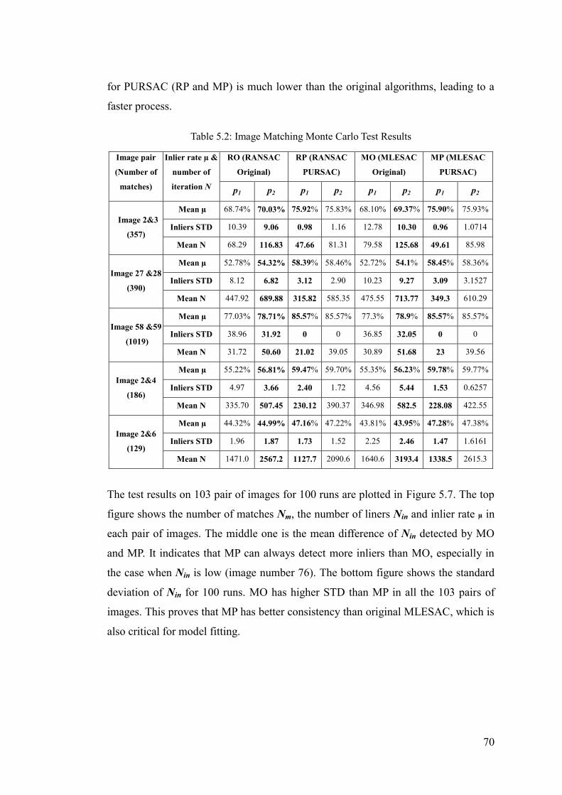
70
for PURSAC (RP and MP) is much lower than the original algorithms, leading to a
faster process.
Table 5.2: Image Matching Monte Carlo Test Results
Image pair
(Number of
matches)
Inlier rate μ &
number of
iteration N
RO (RANSAC
Original)
RP (RANSAC
PURSAC)
MO (MLESAC
Original)
MP (MLESAC
PURSAC)
p1 p2 p1 p2 p1 p2 p1 p2
Image 2&3
(357)
Mean μ 68.74% 70.03% 75.92% 75.83% 68.10% 69.37% 75.90% 75.93%
Inliers STD 10.39 9.06 0.98 1.16 12.78 10.30 0.96 1.0714
Mean N 68.29 116.83 47.66 81.31 79.58 125.68 49.61 85.98
Image 27 &28
(390)
Mean μ 52.78% 54.32% 58.39% 58.46% 52.72% 54.1% 58.45% 58.36%
Inliers STD 8.12 6.82 3.12 2.90 10.23 9.27 3.09 3.1527
Mean N 447.92 689.88 315.82 585.35 475.55 713.77 349.3 610.29
Image 58 &59
(1019)
Mean μ 77.03% 78.71% 85.57% 85.57% 77.3% 78.9% 85.57% 85.57%
Inliers STD 38.96 31.92 0 0 36.85 32.05 0 0
Mean N 31.72 50.60 21.02 39.05 30.89 51.68 23 39.56
Image 2&4
(186)
Mean μ 55.22% 56.81% 59.47% 59.70% 55.35% 56.23% 59.78% 59.77%
Inliers STD 4.97 3.66 2.40 1.72 4.56 5.44 1.53 0.6257
Mean N 335.70 507.45 230.12 390.37 346.98 582.5 228.08 422.55
Image 2&6
(129)
Mean μ 44.32% 44.99% 47.16% 47.22% 43.81% 43.95% 47.28% 47.38%
Inliers STD 1.96 1.87 1.73 1.52 2.25 2.46 1.47 1.6161
Mean N 1471.0 2567.2 1127.7 2090.6 1640.6 3193.4 1338.5 2615.3
The test results on 103 pair of images for 100 runs are plotted in Figure 5.7. The top
figure shows the number of matches Nm, the number of liners Nin and inlier rate μ in
each pair of images. The middle one is the mean difference of Nin detected by MO
and MP. It indicates that MP can always detect more inliers than MO, especially in
the case when Nin is low (image number 76). The bottom figure shows the standard
deviation of Nin for 100 runs. MO has higher STD than MP in all the 103 pairs of
images. This proves that MP has better consistency than original MLESAC, which is
also critical for model fitting.
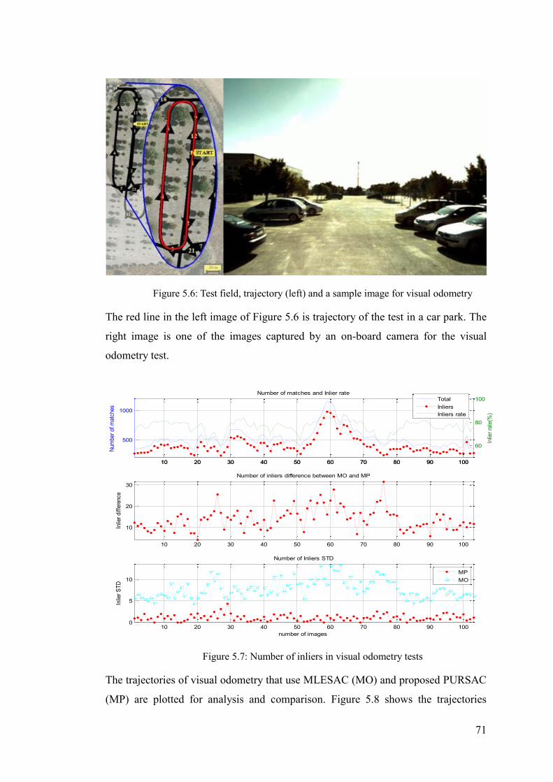
71
Figure 5.6: Test field, trajectory (left) and a sample image for visual odometry
The red line in the left image of Figure 5.6 is trajectory of the test in a car park. The
right image is one of the images captured by an on-board camera for the visual
odometry test.
Figure 5.7: Number of inliers in visual odometry tests
The trajectories of visual odometry that use MLESAC (MO) and proposed PURSAC
(MP) are plotted for analysis and comparison. Figure 5.8 shows the trajectories
10 20 30 40 50 60 70 80 90 100
500
1000
Num
ber o
f mat
ches
Number of matches and Inlier rate
10 20 30 40 50 60 70 80 90 100
60
80
100
Inlie
r rat
e(%
)
TotalInliersInliers rate
10 20 30 40 50 60 70 80 90 100
10
20
30
Inlie
r diff
eren
ce
Number of inliers difference between MO and MP
10 20 30 40 50 60 70 80 90 1000
5
10
number of images
Inlie
r STD
Number of Inliers STD
MPMO
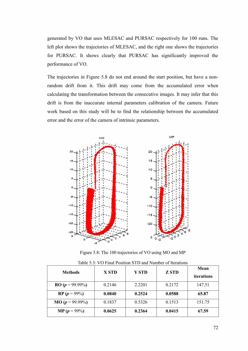
72
generated by VO that uses MLESAC and PURSAC respectively for 100 runs. The
left plot shows the trajectories of MLESAC, and the right one shows the trajectories
for PURSAC. It shows clearly that PURSAC has significantly improved the
performance of VO.
The trajectories in Figure 5.8 do not end around the start position, but have a non-
random drift from it. This drift may come from the accumulated error when
calculating the transformation between the consecutive images. It may infer that this
drift is from the inaccurate internal parameters calibration of the camera. Future
work based on this study will be to find the relationship between the accumulated
error and the error of the camera of intrinsic parameters.
Figure 5.8: The 100 trajectories of VO using MO and MP
Table 5.3: VO Final Position STD and Number of Iterations
Methods X STD Y STD Z STD Mean
iterations
RO (p = 99.99%) 0.2146 2.2201 0.2172 147.51
RP (p = 99%) 0.0840 0.2524 0.0588 65.87
MO (p = 99.99%) 0.1837 0.5326 0.1513 151.75
MP (p = 99%) 0.0625 0.2364 0.0415 67.59
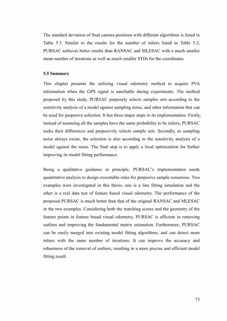
73
The standard deviation of final camera positions with different algorithms is listed in
Table 5.3. Similar to the results for the number of inliers listed in Table 5.2,
PURSAC achieves better results than RANSAC and MLESAC with a much smaller
mean number of iterations as well as much smaller STDs for the coordinates.
5.5 Summary
This chapter presents the utilizing visual odometry method to acquire PVA
information when the GPS signal is unreliable during experiments. The method
proposed by this study, PURSAC purposely selects samples sets according to the
sensitivity analysis of a model against sampling noise, and other information that can
be used for purposive selection. It has three major steps in its implementation. Firstly,
instead of assuming all the samples have the same probability to be inliers, PURSAC
seeks their differences and purposively selects sample sets. Secondly, as sampling
noise always exists, the selection is also according to the sensitivity analysis of a
model against the noise. The final step is to apply a local optimization for further
improving its model fitting performance.
Being a qualitative guidance in principle, PURSAC’s implementation needs
quantitative analysis to design executable rules for purposive sample consensus. Two
examples were investigated in this thesis, one is a line fitting simulation and the
other is a real data test of feature based visual odometry. The performance of the
proposed PURSAC is much better than that of the original RANSAC and MLESAC
in the two examples. Considering both the matching scores and the geometry of the
feature points in feature based visual odometry, PURSAC is efficient in removing
outliers and improving the fundamental matrix estimation. Furthermore, PURSAC
can be easily merged into existing model fitting algorithms, and can detect more
inliers with the same number of iterations. It can improve the accuracy and
robustness of the removal of outliers, resulting in a more precise and efficient model
fitting result.

74
CHAPTER 6 CONCLUSIONS AND
RECOMMENDATIONS
6.1 Conclusions This project has combined varied research fields, such as road surveying, sensors
fusion and computer vision in order to address the challenging topic of real time
exteroceptive sensor data acquisition and processing for an autonomous system. The
system investigated is aimed at giving road maintainers the power to survey road
assets without endangering workers and disrupting traffic. In the past, many
researchers mainly focused on one aspect of road assets surveying without
presenting comprehensive road profiling and surveying results. In the meanwhile, the
recent advances in the resolution of cameras, and LADAR sensors are capable of
providing more accurate and detailed information of surveying objects. The
autonomous system is designed based on sensors fusion (camera, LADAR sensors,
INS, GPS) while LADAR sensors provide dense 3D point clouds of travelling path,
INS generates roll-pitch-yaw motion data of the testing vehicle and GPS presents
continuous position information of the testing vehicle. Camera is utilized in
computer vision for obtaining PVA information, especially in a GPS denied
environment.
Chapter 3 describes the proposed autonomous survey system from its basics. Firstly,
it introduces how the system was constructed and why it was built in such a manner.
The proposed system not only achieves multi-functions, such as road clearance
measurement, road surface profiling, 3D structure modeling, road boundary
detection and road roughness measurement but also operates in a convenient way.
Most importantly, data collected by sensors has less chance of being blocked by
other vehicles in a complex driving environment. Secondly, hardware consist of two
LADAR sensors, one IMU, one GPS and one camera, which are mounted on the
designed aluminum integrated sensors frame and then installed at the back of a
vehicle at a proper height (2300 mm). The feasibility and stability of the manner of
sensors installation has been developed after many driving tests. Thirdly, a real-time
acquisition software for receiving and recording data from LADAR sensors and IMU
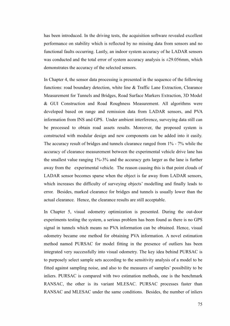
75
has been introduced. In the driving tests, the acquisition software revealed excellent
performance on stability which is reflected by no missing data from sensors and no
functional faults occurring. Lastly, an indoor system accuracy of he LADAR sensors
was conducted and the total error of system accuracy analysis is ±29.056mm, which
demonstrates the accuracy of the selected sensors.
In Chapter 4, the sensor data processing is presented in the sequence of the following
functions: road boundary detection, white line & Traffic Lane Extraction, Clearance
Measurement for Tunnels and Bridges, Road Surface Markers Extraction, 3D Model
& GUI Construction and Road Roughness Measurement. All algorithms were
developed based on range and remission data from LADAR sensors, and PVA
information from INS and GPS. Under ambient interference, surveying data still can
be processed to obtain road assets results. Moreover, the proposed system is
constructed with modular design and new components can be added into it easily.
The accuracy result of bridges and tunnels clearance ranged from 1% - 7% while the
accuracy of clearance measurement between the experimental vehicle drive lane has
the smallest value ranging 1%-3% and the accuracy gets larger as the lane is further
away from the experimental vehicle. The reason causing this is that point clouds of
LADAR sensor becomes sparse when the object is far away from LADAR sensors,
which increases the difficulty of surveying objects’ modelling and finally leads to
error. Besides, marked clearance for bridges and tunnels is usually lower than the
actual clearance. Hence, the clearance results are still acceptable.
In Chapter 5, visual odometry optimization is presented. During the out-door
experiments testing the system, a serious problem has been found as there is no GPS
signal in tunnels which means no PVA information can be obtained. Hence, visual
odometry became one method for obtaining PVA information. A novel estimation
method named PURSAC for model fitting in the presence of outliers has been
integrated very successfully into visual odometry. The key idea behind PURSAC is
to purposely select sample sets according to the sensitivity analysis of a model to be
fitted against sampling noise, and also to the measures of samples’ possibility to be
inliers. PURSAC is compared with two estimation methods, one is the benchmark
RANSAC, the other is its variant MLESAC. PURSAC processes faster than
RANSAC and MLESAC under the same conditions. Besides, the number of inliers
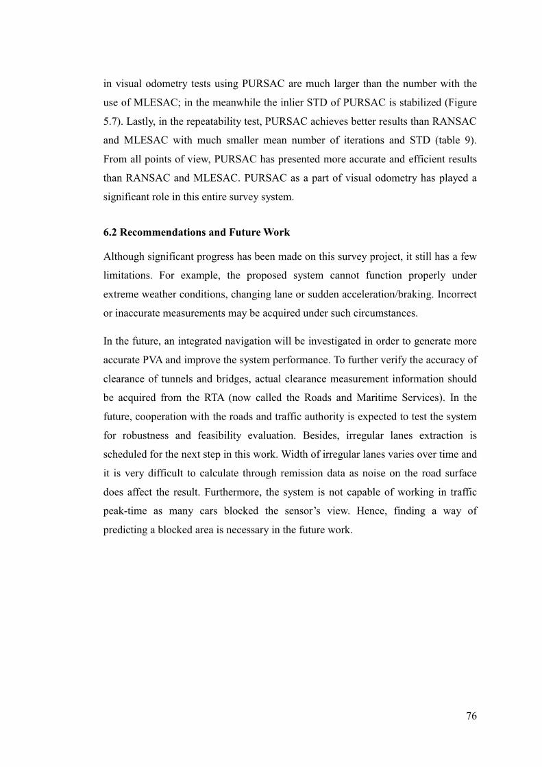
76
in visual odometry tests using PURSAC are much larger than the number with the
use of MLESAC; in the meanwhile the inlier STD of PURSAC is stabilized (Figure
5.7). Lastly, in the repeatability test, PURSAC achieves better results than RANSAC
and MLESAC with much smaller mean number of iterations and STD (table 9).
From all points of view, PURSAC has presented more accurate and efficient results
than RANSAC and MLESAC. PURSAC as a part of visual odometry has played a
significant role in this entire survey system.
6.2 Recommendations and Future Work Although significant progress has been made on this survey project, it still has a few
limitations. For example, the proposed system cannot function properly under
extreme weather conditions, changing lane or sudden acceleration/braking. Incorrect
or inaccurate measurements may be acquired under such circumstances.
In the future, an integrated navigation will be investigated in order to generate more
accurate PVA and improve the system performance. To further verify the accuracy of
clearance of tunnels and bridges, actual clearance measurement information should
be acquired from the RTA (now called the Roads and Maritime Services). In the
future, cooperation with the roads and traffic authority is expected to test the system
for robustness and feasibility evaluation. Besides, irregular lanes extraction is
scheduled for the next step in this work. Width of irregular lanes varies over time and
it is very difficult to calculate through remission data as noise on the road surface
does affect the result. Furthermore, the system is not capable of working in traffic
peak-time as many cars blocked the sensor’s view. Hence, finding a way of
predicting a blocked area is necessary in the future work.

77
LIST OF PUBLICATIONS
[1] X. T. Ren, X. Luo, and J. J. Wang, “Automatic Road Clearance Surveying with
Sensor Fusion”, Australasian Conference on Robotics and Automation (ACRA),
Melbourne, December 2011.
[2] X. Luo, X. T. Ren, Y. Li, J. J. Wang, “Mobile Surveying System for Road Assets
Monitoring and Management”, IEEE Conference on Industrial Electronics and
Applications (ICIEA, Singapore, July 2012.
[3] Y. Li, X. Luo, X. T. Ren and J. J. Wang, “A Robust Humanoid Robot Navigation
Algorithm with ZUPT”, IEEE International Conference on Mechatronics and
Automation (ICMA), Chengdu, China, August 2012
[4] X. Luo, Y. Li, X. T. Ren, and J. J. Wang,” Automatic Road Surface Profiling with
Sensors Fusion”,12th International Conference on Control, Automation, Robotics
and Vision (ICARCV), 2012.
[5] Y. Li, X. Luo, J. J. Wang and S. Xiao,” Dead Reckoning Navigation with
Constant Velocity Update (CUPT)”,12th International Conference on Control,
Automation, Robotics and Vision (ICARCV), 2012.
[6] J. J. Wang and X. Luo, ”Purposive Sample Consensus: A Paradigm for Model
Fitting with Application to Visual Odometry”, The 9th Conference on Field and
Service Robotics (FSR) December 9-11, 2013, Brisbane. (Accepted)
78
REFERENCES
[1] A. Waheed and M. Caya ’’High Speed Geo-referenced Bridge Clearance Data
Collection at Ohio Dot’’, 2006 GIS-T Symposium Columbus Ohio, viewed at:
http://www.gis-t.org/files/Pi1Hj.pdf
[2] W. S. Wijesoma, K. R. S Kodagoda and A. P. Balasuriya, “Road-boundary
Detection and Tracking Using LADAR Sensing’’, Robotics and Automation,
IEEE Transactions on, 2004, 20(3): 456-464.
[3] F. Oniga, R. Danescu and S. Nedevschi, “Mixed Road Surface Model for
Driving Assistance Systems”, Intelligent Computer Communication and
Processing (ICCP), 2010 IEEE International Conference on. IEEE, 2010: 185-
190.
[4] T. H. Hong, C. Rasmussen, T. Chang and et al, “Road Detection and Tracking
for Autonomous Mobile Robots”, AeroSense 2002. International Society for
Optics and Photonics, 2002: 311-319.
[5] M. Doumiati, A. Victorino, A. Charara and et al, “Estimation of Road Profile
for Vehicle Dynamics Motion: Experimental Validation”, American Control
Conference (ACC), 2011. IEEE, 2011: 5237-5242.
[6] D. Scaramuzza and F. Fraundorfer, “Visual Odometry [tutorial]”, Robotics &
Automation Magazine, IEEE, 2011, 18(4): 80-92.
[7] X. Jin and C. H. Davis, “An Integrated System for Automatic Road Mapping
from High-resolution Multi-spectral Satellite Imagery by Information Fusion”,
Information Fusion, 2005, 6(4): 257-273.
[8] E. B. Olson, S. Teller and J. Leonard, “Robust and Efficient Robotic Mapping”,
Massachusetts Institute of Technology, Department of Electrical Engineering
and Computer Science, 2008.
[9] J. Dong, D. Zhuang, Y. Huang and et al, “Advances in Multi-Sensor Data
Fusion: Algorithms and Applications”, Sensors, 2009, 9(10): 7771-7784.
[10] P. Doucette, P. Agouris and A. Stefanidis. “Automated Road Extraction from
High Resolution Multispectral Imagery”, Photogrammetric Engineering &
Remote Sensing, 2004, 70(12): 1405-1416.

79
[11] Kukko, A. Jaakkola, M. Lehtomaki, and et al, “Mobile Mapping System and
Computing Methods for Modelling of Road Environment”, Urban Remote
Sensing Event, 2009 Joint. IEEE, 2009: 1-6.
[12] Y. Lin, J. Hyyppa and A. Jaakkola, “Mini-UAV-borne LIDAR for Fine-scale
Mapping”, Geoscience and Remote Sensing Letters, IEEE, 2011, 8(3): 426-430.
[13] Y. Hu, “Automated Extraction of Digital Terrain Models, Roads and Buildings
Using Airborne LIDAR Data”, 2004.
[14] D. R. Entriken and C. Rizos, “Application of Mobile Mapping Technology
within a Roads and Traffic Authority”, International Global Navigation
Satellite Systems Society IGNSS Symposium. 2007.
[15] Y. Shi, R. Shibasaki and Z. Shi, “Towards Automatic Road Mapping by Fusing
Vehicle-Borne Multi-Sensor Data”, Int. Arch. Photogram. Rem. Sens. Spatial
Inform. Sci, 2008, 37: 867-872.
[16] G. Sohn and I. Dowman, “Data Fusion of High-Resolution Satellite Imagery
and LIDAR Data for Automatic Building Extraction”, ISPRS Journal of
Photogrammetry and Remote Sensing, 2007, 62(1): 43-63.
[17] B. Ma, S. Lakshmanan and A. O. Hero III, “Simultaneous Detection of Lane
and Pavement Boundaries Using Model-based Multi-sensor Fusion”, Intelligent
Transportation Systems, IEEE Transactions on, 2000, 1(3): 135-147.
[18] M. Hu, W. Yang, M. Ren and et al, “A Vision Based Road Detection Algorithm”,
Robotics, Automation and Mechatronics, 2004 IEEE Conference on. IEEE,
2004, 2: 846-850.
[19] F. Homm, N. Kaempchen, J. Ota and et al, “Efficient Occupancy Grid
Computation on the GPU with LIDAR and Radar for Road Boundary
Detection”, Intelligent Vehicles Symposium (IV), 2010 IEEE. IEEE, 2010: 1006-
1013.
[20] C. Guo, S. Mita and D. McAllester, “Stereovision-based Road Boundary
Detection for Intelligent Vehicles in Challenging Scenarios”, Intelligent Robots
and Systems, 2009. IROS 2009. IEEE/RSJ International Conference on. IEEE,
2009: 1723-1728.
[21] Y. Yamaguchi, M. Sengoku and S. Motooka, “Using Van-mounted FM-CW
Radar to Detect Corner-reflector Road-boundary Markers”, Instrumentation and
Measurement, IEEE Transactions on, 1996, 45(4): 793-799.

80
[22] M. Darms, M. Komar and S. Lueke, “Map Based Road Boundary Estimation”,
Intelligent Vehicles Symposium (IV), 2010 IEEE. IEEE, 2010: 609-614.
[23] Y. Wang, E. K. Teoh and D. Shen, “Lane Detection and Tracking Using B-
Snake”, Image and Vision computing, 2004, 22(4): 269-280.
[24] K. M. Wurm, R. Kummerle, C. Stachniss and et al, “Improving robot
Navigation in Structured Outdoor Environments by Identifying Vegetation from
Laser Data”, Intelligent Robots and Systems, 2009. IROS 2009. IEEE/RSJ
International Conference on. IEEE, 2009: 1217-1222.
[25] H. Lin, H. Kim, C. Lin and et al, “Road Boundary Detection Based on the
Dynamic Programming and the Randomized Hough Transform”, Information
Technology Convergence, 2007. ISITC 2007. International Symposium on.
IEEE, 2007: 63-70.
[26] H. Kong, J. Y. Audibert and J. Ponce, “General Road Detection from a Single
Image”, Image Processing, IEEE Transactions on, 2010, 19(8): 2211-2220.
[27] T. Saitoh and Y. Kuroda, “Online Road Surface Analysis Using Laser
Remission Value in Urban Environments”, Intelligent Robots and Systems
(IROS), 2010 IEEE/RSJ International Conference on. IEEE, 2010: 15-21.
[28] M. W. Sayers, “Profiles of Roughness”, Transportation Research Record, 1990
(1260).
[29] M. W. Sayers, “On the Calculation of International Roughness Index from
Longitudinal Road Profile”, Transportation Research Record, 1995 (1501): 1-
12.
[30] vueworks, “Efficient Measurement of Bridge and Overhead Structure Clearance
Information at Posted Highway Speeds”, viewed at
http://vueworks.com/efficient-measurement-of-bridge-and-overhead-structure-
clearance-information-at-posted-highway-speeds-2/
[31] F. Fraundorfer and D. Scaramuzza, "Visual Odometry Part II: Matching,
Robustness, Optimization, and Applications," Robotics & Automation
Magazine, IEEE, vol. 19, pp. 78-90, 2012.
[32] M. A. Fischler and R. C. Bolles, "Random sample Consensus: A Paradigm for
Model Fitting with Applications to Image Analysis and Automated
Cartography," Communications of the ACM, vol. 24, pp. 381-395, 1981.
81
[33] D. Nister, "Preemptive RANSAC for Live Structure and Motion Estimation," in
Computer Vision, 2003. Proceedings. Ninth IEEE International Conference on,
2003, pp. 199-206 vol.1.
[34] D. Nister, "An Efficient Solution to the Five-Point Relative Pose Problem,"
Pattern Analysis and Machine Intelligence, IEEE Transactions on, vol. 26, pp.
756-770, 2004.
[35] J. M. Frahm and M. Pollefeys, "RANSAC for (quasi-) degenerate data
(QDEGSAC)," in Computer Vision and Pattern Recognition, 2006 IEEE
Computer Society Conference on, 2006, pp. 453-460.
[36] N. Kai, et al., "GroupSAC: Efficient Consensus in the Presence of Groupings,"
in Computer Vision, 2009 IEEE 12th International Conference on, 2009, pp.
2193-2200.
[37] E. Rosten, et al., "Improved RANSAC performance Using Simple, Iterative
Minimal-set Solvers," arXiv preprint arXiv: 1007.1432, 2010.
[38] P. H. S. Torr and A. Zisserman, "MLESAC: A New Robust Estimator with
Application to Estimating Image Geometry," Computer Vision and Image
Understanding, vol. 78, pp. 138-156, 2000.
[39] O. Chum and J. Matas, "Matching with PROSAC - Progressive Sample
Consensus," in Computer Vision and Pattern Recognition, CVPR 2005. IEEE
Computer Society Conference on, 2005, pp. 220-226 vol. 1.
[40] D. Capel, "An effective bail-out test for RANSAC consensus scoring," in Proc.
BMVC, 2005, pp. 629-638.
[41] D. Scaramuzza, F. Fraundorfer, and R. Siegwart, “Real-time Monocular Visual
Odometry for On-Road Vehicles With 1-point RANSAC,” in Proc. IEEE Int.
Conf. Robotics and Automation (ICRA), 2009, pp. 4293–4299.
[42] D. Nister, O. Naroditsky, and J. Bergen, “Visual Odometry,” in Proc. Int. Conf.
Computer Vision and Pattern Recognition, 2004, pp. 652–659.
[43] R. Raguram, J. Frahm, and M. Pollefeys, “Exploiting Uncertainty in Random
Sample Consensus,” in Proc. ICCV, 2009, pp. 2074–2081.
[44] P. McIlroy, E. Rosten, S. Taylor, and T. Drummond, “Deterministic Sample
Consensus with Multiple Match Hypotheses,” in Proc. British Machine Vision
Conf. 2010, pp. 1–11.
82
[45] Volker Rodehorst and Olaf Hellwich, "Genetic Algorithm SAmple Consensus
(GASAC) - A Parallel Strategy for Robust Parameter Estimation", in
Proceedings of the 2006 Conference on Computer Vision and Pattern
Recognition Workshop (CVPRW’06), 17-22 June 2006, pp. 103-111.
[46] SICK, 2009, LMS111 Laser Measurement System Operating Instructions,
viewed at:
https://mysick.com/eCat.aspx?go=Finder&Cat=Row&At=Fa&Cult=English&C
ategory=Produktfinder
[47] SICK, 2011, LMS400 Laser Measurement System Operating Instructions,
viewed at:
https://mysick.com/eCat.aspx?go=Finder&Cat=Row&At=Fa&Cult=English&C
ategory=Produktfinder
[48] J. Weingarten, “Feature-based 3D SLAM”, ÉCOLE POLYTECHNIQUE
FÉDÉRALE DE LAUSANNE, 2006.
[49] Q. F. Yu, H. W. Lu and X. L. Liu, “Accurate Measurement and Dynamic
Measurement Based on Moving Graph”, Science Press, 2002.
[50] RTA, 2011a, “Safety in Sydney’s Major Road Tunnel”, viewed at
http://www.rta.nsw.gov.au/usingroads/downloads/tunnel_safety_dl1.html
[51] RTA, 2011b, “Over-height Vehicles, Fact Sheet for Operators” viewed at
http://www.rta.nsw.gov.au/
[52] S. M. Lavalle, Planning Algorithm, Cambridge University Press, viewed at
http://planning.cs.uiuc.edu/node102.html
Acuity Laser Sensors (Schmitt Industries) 2012, “High speed, Longitudinal
Road Profiling”, viewed at: http://www.acuitylaser.com/AR700/common-
applications-road-profiling- sensor.html
[53] M.W. Sayers and S.M. Karamihas, :The Little Book of Profiling”, 1998,
University of Michigan Transport Research Institute, viewed at:
http://www.umtri.umich.edu/content/LittleBook98R.pdf
[55] H. Bay, T. Tuytelaars and L. Van Gool, “Surf: Speeded up Robust Features”,
Computer Vision–ECCV 2006, Springer Berlin Heidelberg, 2006: 404-417.
[56] D. Lowe, “Distinctive Image Features from Scale-Invariant Key Points”,
International Journal of Computer Vision, vol. 20, no. 2, pp. 91–110, 2003.
83
[57] Jose-Luis Blanco, Francisco-Angel Moreno, Javier Gonzalez, “A Collection of
Outdoor Robotic Datasets with centimeter-accuracy Ground Truth”,
Autonomous Robots, 2009. Volume 27, Issue 4, pp. 327-351.
[58] J.J. Wang, S. Kodagoda, G. Dissanayake, “Vision Aided GPS/INS System for
Robust Land Vehicle Navigation”, Proceedings of the 22nd International
Technical Meeting of The Satellite Division of the Institute of Navigation (ION
GNSS 2009), Savannah, Georgia, USA, 22-25 September 2009, pp.600 - 609.
[59] L. Zhao, S.D. Huang, L. Yan, J.J. Wang, G. Hu and G. Dissanayake, “Large-
Scale Monocular SLAM by Local Bundle Adjustment and Map Joining”, in
Proc. of the 11th. Int. Conf. Control, Automation, Robotics and Vision
(ICARCV 2010), ed IEEE Technical Committee, IEEE, Singapore, December
2010, pp. 431-436.
[60] O. Chum, J. Matas, and J. Kittler, “Locally optimized RANSAC,” in Proc.
DAGM- Symposium, pp. 236–243, 2003.
[61] Ben Tordoff and David W Murray, “Guided Sampling and Consensus for Motion Estimation”, Computer Vision—ECCV 2002, - Springer
[62] J. M. B. Dalibard, D. Kaplan. “GPS & Selective Availability Q&A”. White paper.
[63] E. G. Blackwell. “Overview of Differential GPS Methods”, Navigation, 1985, 32(2): 114-125.
[64] J. A. Corrales, F. A. Candelas and F. Torres, “Hybrid Tracking of Human Operators Using IMU/UWB Data Fusion by a Kalman Filter”, Human-Robot Interaction (HRI), 2008 3rd ACM/IEEE International Conference on. IEEE, 2008: 193-200.
[65] Simulated Realty, “Odometry”, Viewed on 27th October 2013 at:
http://simreal.com/content/Odometry
[66] Y .Cheng, M. W. Maimone and L . Matthies, “Visual Odometry on the Mars Exploration Rovers-A Tool to Ensure Accurate Driving and Science Imaging”. Robotics & Automation Magazine, IEEE, 2006, 13(2): 54-62.
[67] F. Caron, E. Duflos, D. Pomorski and et al, “GPS/IMU Data Fusion Using Multi-sensor Kalman Filtering: Introduction of Contextual Aspects”, Information Fusion, 2006, 7(2): 221-230.
[68] J. A. Rios and E. White, “Fusion Filter Algorithm Enhancements for a MEMS GPS/IMU”, ION NTM. 2002: 28-30.
[69] M. A. Batalin, G. S. Sukhatme and M. Hattig, “Mobile Robot Navigation Using a Sensor Network”, Robotics and Automation, 2004. Proceedings. ICRA'04. 2004 IEEE International Conference on. IEEE, 2004, 1: 636-641.

84
[70] M. A. Lefsky, W. B. Cohen, G. G. Parker and et al, “Lidar Remote Sensing for Ecosystem Studies”, BioScience, 2002, 52(1): 19-30.
[71] J. B. Campbell, “Introduction to remote sensing”, Taylor & Francis, 2002.
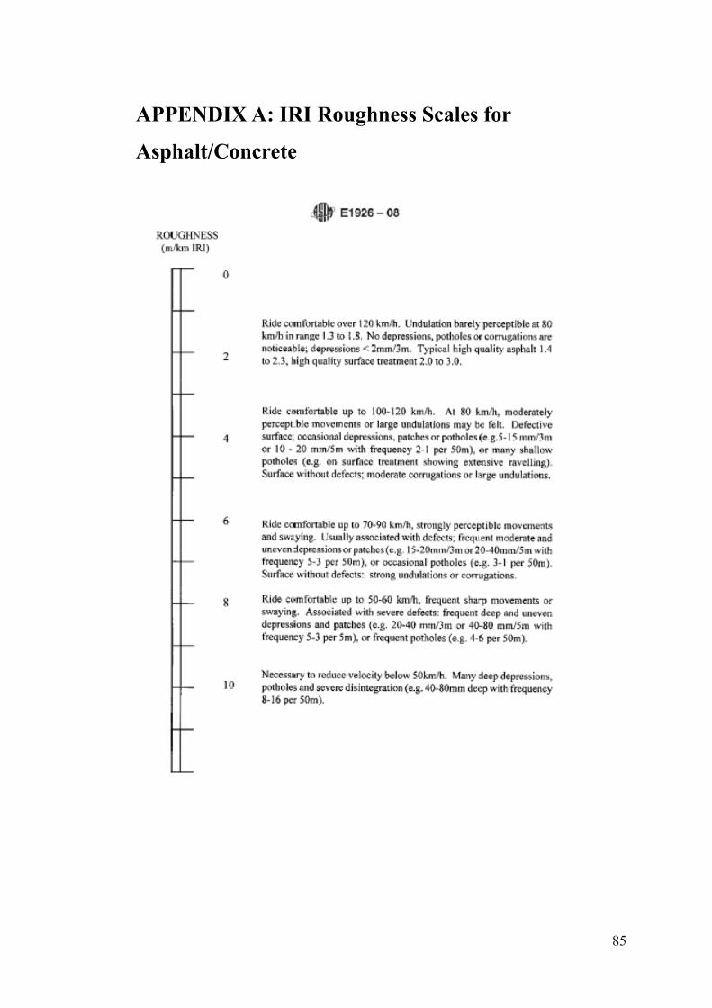
85
APPENDIX A: IRI Roughness Scales for
Asphalt/Concrete
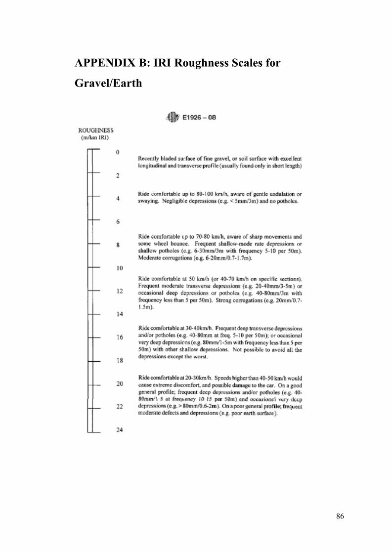
86
APPENDIX B: IRI Roughness Scales for
Gravel/Earth
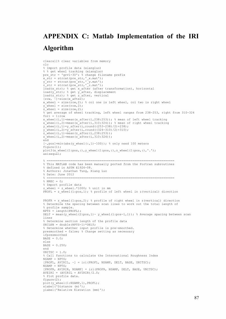
87
APPENDIX C: Matlab Implementation of the IRI
Algorithm
clearall% clear variables from memory clc % Import profile data (xiangluo) % % get wheel tracking (xiangluo) pre_str = 'grv1-30'; % change filename prefix x_str = strcat(pre_str,'_x.mat'); y_str = strcat(pre_str,'_y.mat'); z_str = strcat(pre_str,'_z.mat'); load(x_str); % get x_after (after transformation), horizontal load(y_str); % get y_after, displacement load(z_str); % get z_after, vertical [row, ~]=size(x_after); x_wheel = size(row,2); % col one is left wheel, col two is right wheel y_wheel = size(row,2); z_wheel = size(row,2); % get average of wheel tracking, left wheel ranges from 238-253, right from 310-324 fori = 1:row x_wheel(i,1)=mean(x_after(i,238:253)); % mean of left wheel tracking x_wheel(i,2)=mean(x_after(i,310:324)); % mean of right wheel tracking y_wheel(i,1)=y_after(i,round((253-238)/2)+238); y_wheel(i,2)=y_after(i,round((324-310)/2)+310); z_wheel(i,1)=mean(z_after(i,238:253)); z_wheel(i,2)=mean(z_after(i,310:324)); end [~,pos]=min(abs(y_wheel(:,1)-100)); % only need 100 meters figure(1); plot3(x_wheel(1:pos,:),y_wheel(1:pos,:),z_wheel(1:pos,:),'.'); axisequal; % ====================================================================== % This MATLAB code has been manually ported from the Fortran subroutines % defined in ASTM E1926-08. % Authors: Jonathan Tung, Xiang Luo % Date: June 2012 % ====================================================================== % NREC = 0; % Import profile data z_wheel = z_wheel.*1000; % unit in mm PROFL = z_wheel(1:pos,1); % profile of left wheel in z(vertical) direction
PROFR = z_wheel(1:pos,2); % profile of right wheel in z(vertical) direction % Determine the spacing between scan lines to work out the total length of % profile sample. NPTS = length(PROFL); DELT = mean(y_wheel(2:pos,1)- y_wheel(1:pos-1,1)); % Average spacing between scan lines % Determine section length of the profile data SECLEN = double(NPTS-1)*DELT; % Determine whether input profile is pre-smoothed. presmoothed = false; % Change setting as necessary ifpresmoothed BASE = 0.0; else BASE = 0.250; end UNITSC = 1.0; % Call functions to calculate the International Roughness Index NSAMP = NPTS; [PROFL, AVIRIL, ~] = iri(PROFL, NSAMP, DELT, BASE, UNITSC); NSAMP = NPTS; [PROFR, AVIRIR, NSAMP] = iri(PROFR, NSAMP, DELT, BASE, UNITSC); AVEIRI = (AVIRIL + AVIRIR)/2.0; % Plot profile data. figure(2); plot(y_wheel(1:NSAMP,1),PROFL); xlabel('Distance (m)'); ylabel('Relative Elevation (mm)');
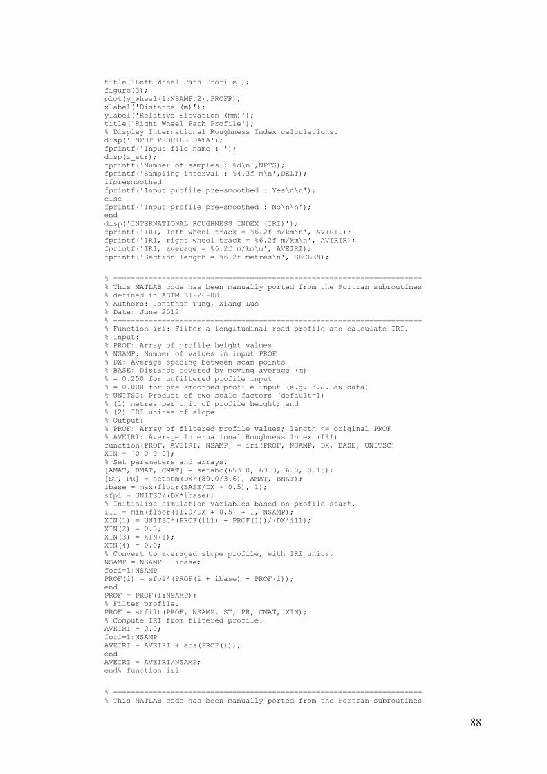
88
title('Left Wheel Path Profile'); figure(3); plot(y_wheel(1:NSAMP,2),PROFR); xlabel('Distance (m)'); ylabel('Relative Elevation (mm)'); title('Right Wheel Path Profile'); % Display International Roughness Index calculations. disp('INPUT PROFILE DATA'); fprintf('Input file name : '); disp(z_str); fprintf('Number of samples : %d\n',NPTS); fprintf('Sampling interval : %4.3f m\n',DELT); ifpresmoothed fprintf('Input profile pre-smoothed : Yes\n\n'); else fprintf('Input profile pre-smoothed : No\n\n'); end disp('INTERNATIONAL ROUGHNESS INDEX (IRI)'); fprintf('IRI, left wheel track = %6.2f m/km\n', AVIRIL); fprintf('IRI, right wheel track = %6.2f m/km\n', AVIRIR); fprintf('IRI, average = %6.2f m/km\n', AVEIRI); fprintf('Section length = %6.2f metres\n', SECLEN);
% ====================================================================== % This MATLAB code has been manually ported from the Fortran subroutines % defined in ASTM E1926-08. % Authors: Jonathan Tung, Xiang Luo % Date: June 2012 % ====================================================================== % Function iri: Filter a longitudinal road profile and calculate IRI. % Input: % PROF: Array of profile height values % NSAMP: Number of values in input PROF % DX: Average spacing between scan points % BASE: Distance covered by moving average (m) % = 0.250 for unfiltered profile input % = 0.000 for pre-smoothed profile input (e.g. K.J.Law data) % UNITSC: Product of two scale factors (default=1) % (1) metres per unit of profile height; and % (2) IRI unites of slope % Output: % PROF: Array of filtered profile values; length <= original PROF % AVEIRI: Average International Roughness Index (IRI) function[PROF, AVEIRI, NSAMP] = iri(PROF, NSAMP, DX, BASE, UNITSC) XIN = [0 0 0 0]; % Set parameters and arrays. [AMAT, BMAT, CMAT] = setabc(653.0, 63.3, 6.0, 0.15); [ST, PR] = setstm(DX/(80.0/3.6), AMAT, BMAT); ibase = max(floor(BASE/DX + 0.5), 1); sfpi = UNITSC/(DX*ibase); % Initialise simulation variables based on profile start. i11 = min(floor(11.0/DX + 0.5) + 1, NSAMP); XIN(1) = UNITSC*(PROF(i11) - PROF(1))/(DX*i11); XIN(2) = 0.0; XIN(3) = XIN(1); XIN(4) = 0.0; % Convert to averaged slope profile, with IRI units. NSAMP = NSAMP - ibase; fori=1:NSAMP PROF(i) = sfpi*(PROF(i + ibase) - PROF(i)); end PROF = PROF(1:NSAMP); % Filter profile. PROF = stfilt(PROF, NSAMP, ST, PR, CMAT, XIN); % Compute IRI from filtered profile. AVEIRI = 0.0; fori=1:NSAMP AVEIRI = AVEIRI + abs(PROF(i)); end AVEIRI = AVEIRI/NSAMP; end% function iri % ====================================================================== % This MATLAB code has been manually ported from the Fortran subroutines
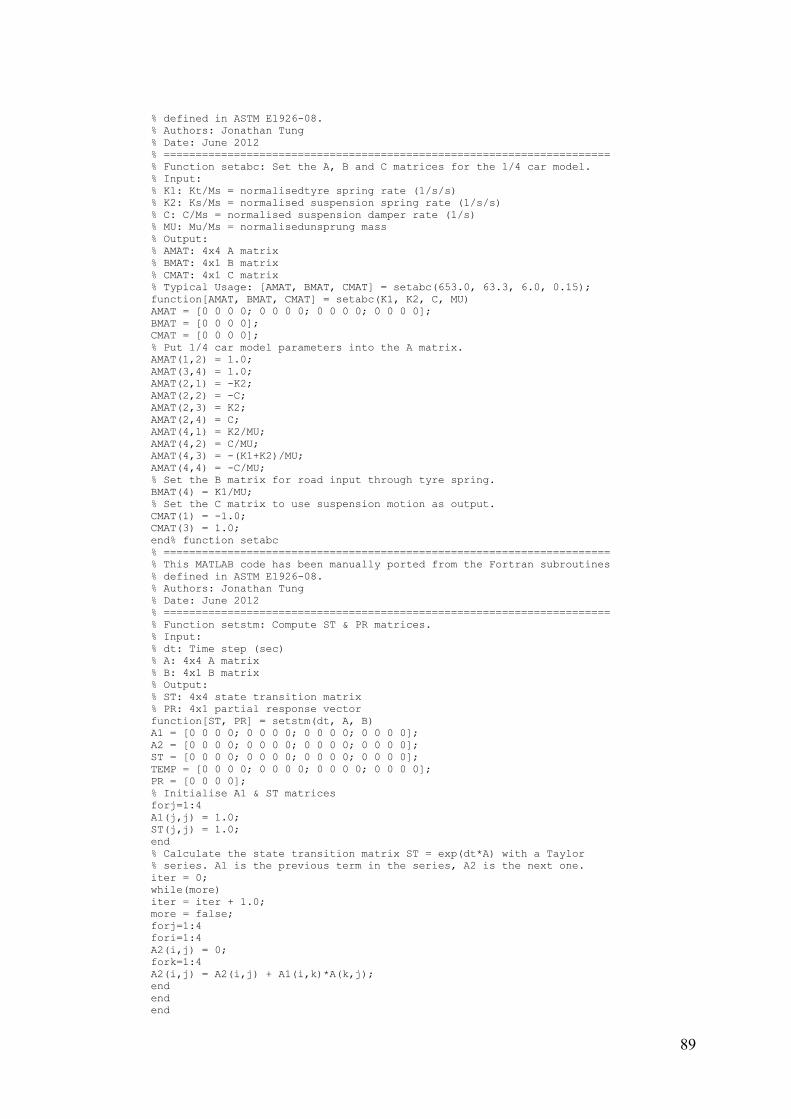
89
% defined in ASTM E1926-08. % Authors: Jonathan Tung % Date: June 2012 % ====================================================================== % Function setabc: Set the A, B and C matrices for the 1/4 car model. % Input: % K1: Kt/Ms = normalisedtyre spring rate (1/s/s) % K2: Ks/Ms = normalised suspension spring rate (1/s/s) % C: C/Ms = normalised suspension damper rate (1/s) % MU: Mu/Ms = normalisedunsprung mass % Output: % AMAT: 4x4 A matrix % BMAT: 4x1 B matrix % CMAT: 4x1 C matrix % Typical Usage: [AMAT, BMAT, CMAT] = setabc(653.0, 63.3, 6.0, 0.15); function[AMAT, BMAT, CMAT] = setabc(K1, K2, C, MU) AMAT = [0 0 0 0; 0 0 0 0; 0 0 0 0; 0 0 0 0]; BMAT = [0 0 0 0]; CMAT = [0 0 0 0]; % Put 1/4 car model parameters into the A matrix. AMAT(1,2) = 1.0; AMAT(3,4) = 1.0; AMAT(2,1) = -K2; AMAT(2,2) = -C; AMAT(2,3) = K2; AMAT(2,4) = C; AMAT(4,1) = K2/MU; AMAT(4,2) = C/MU; AMAT(4,3) = -(K1+K2)/MU; AMAT(4,4) = -C/MU; % Set the B matrix for road input through tyre spring. BMAT(4) = K1/MU; % Set the C matrix to use suspension motion as output. CMAT(1) = -1.0; CMAT(3) = 1.0; end% function setabc % ====================================================================== % This MATLAB code has been manually ported from the Fortran subroutines % defined in ASTM E1926-08. % Authors: Jonathan Tung % Date: June 2012 % ====================================================================== % Function setstm: Compute ST & PR matrices. % Input: % dt: Time step (sec) % A: 4x4 A matrix % B: 4x1 B matrix % Output: % ST: 4x4 state transition matrix % PR: 4x1 partial response vector function[ST, PR] = setstm(dt, A, B) A1 = [0 0 0 0; 0 0 0 0; 0 0 0 0; 0 0 0 0]; A2 = [0 0 0 0; 0 0 0 0; 0 0 0 0; 0 0 0 0]; ST = [0 0 0 0; 0 0 0 0; 0 0 0 0; 0 0 0 0]; TEMP = [0 0 0 0; 0 0 0 0; 0 0 0 0; 0 0 0 0]; PR = [0 0 0 0]; % Initialise A1 & ST matrices forj=1:4 A1(j,j) = 1.0; ST(j,j) = 1.0; end % Calculate the state transition matrix ST = exp(dt*A) with a Taylor % series. A1 is the previous term in the series, A2 is the next one. iter = 0; while(more) iter = iter + 1.0; more = false; forj=1:4 fori=1:4 A2(i,j) = 0; fork=1:4 A2(i,j) = A2(i,j) + A1(i,k)*A(k,j); end end end
90
forj=1:4 fori=1:4 A1(i,j) = A2(i,j)*dt/iter; if((ST(i,j) + A1(i,j)) ~= ST(i,j)) more = true; end ST(i,j) = ST(i,j) + A1(i,j); end end end % Calculate particular response matrix: PR = A**-1*(ST-I)*B % A = invert(A, 4); A = inv(A); % native MATLAB matrix inversion function for speed fori=1:4 PR(i) = 0.0; fork=1:4 PR(i) = PR(i) - A(i,k)*B(k); end end forj=1:4 fori=1:4 TEMP(j,i) = 0.0; fork=1:4 TEMP(j,i) = TEMP(j,i) + A(j,k)*ST(k,i); end end fork=1:4 PR(j) = PR(j) + TEMP(j,k)*B(k); end end end% function setstm % ====================================================================== % This MATLAB code has been manually ported from the Fortran subroutines % defined in ASTM E1926-08. % Authors: Jonathan Tung % Date: June 2012 % ====================================================================== % Function stfilt: Filter profile using matrices ST & PR % Input: % PROF: Input profile % NSAMP: Number of data values in array PROF % ST: 4x4 state transition matrix % PR: 4x1 partial response matrix % C: 4x1 output definition values % XIN: Initial values of filtered variables % Output: % PROF: Filtered profile. Overwrites input profile. functionPROF = stfilt(PROF, NSAMP, ST, PR, C, XIN) X = [0 0 0 0]; XN = [0 0 0 0];
% Initialise simulation variables. fori=1:4 X(i) = XIN(i); end % Filter profile using the state transition algorithm. fori=1:NSAMP forj=1:4 XN(j) = PR(j)*PROF(i); fork=1:4 XN(j) = XN(j) + X(k)*ST(j,k); end end forj=1:4 X(j) = XN(j); end PROF(i) = X(1)*C(1) + X(2)*C(2) + X(3)*C(3) + X(4)*C(4); end end% function stfilt % ====================================================================== % This MATLAB code has been manually ported from the Fortran subroutines % defined in ASTM E1926-08. % Authors: Jonathan Tung % Date: June 2012
91
% ====================================================================== % Function invert: Returns the inverse of NxN matrix Y1. % Algorithm adapted from ASTM E1926-08 and "Numerical Recipes in % Fortran 77". % http://www.mpi-hd.mpg.de/astrophysik/HEA/internal/Numerical_Recipes/f2-3. % pdf % Input: % Y1: Input matrix % N: Dimension of NxN matrix % Output: % Y1: The inverse of input matrix Y1 functionY1 = invert(Y1, N) A = [0 0 0 0; 0 0 0 0; 0 0 0 0; 0 0 0 0]; YINV = [0 0 0 0; 0 0 0 0; 0 0 0 0; 0 0 0 0]; fori=1:N forj=1:N A(i,j) = Y1(i,j); end end fori=1:N forj=1:N YINV(i,j) = 0.0; end YINV(i,i) = 1.0; end % LU matrix decomposition [A, INDX] = ludcmp(A); % modified ludcmp function % LU matrix back substitution YINV = lubksb(A, INDX, YINV); % modified lubksb function fori=1:N forj=1:N Y1(i,j) = YINV(i,j); end end end% function invert
% ====================================================================== % This MATLAB code has been manually ported from the Fortran subroutines % defined in ASTM E1926-08. % Authors: Jonathan Tung % Date: June 2012 % ====================================================================== % Function ludcmp: LU matrix decomposition % Algorithm adapted from ASTM E1926-08 and "Numerical Recipes in % Fortran 77". % http://www.mpi-hd.mpg.de/astrophysik/HEA/internal/Numerical_Recipes/f2-3. % pdf % Input: % A: 4x4 A matrix % Output: % A: 4x4 A matrix % INDX: 4x1 matrix function[A, INDX] = ludcmp(A) NMAX = 100; VV = zeros(1,NMAX); TINY=1.0e-20; N=4; INDX = zeros(1,N); IMAX = 0; D=1.0; fori=1:N AAMAX = 0.0; forj=1:N ifabs(A(i,j)) > AAMAX AAMAX = abs(A(i,j)); end end ifAAMAX == 0.0 warning('Singular matrix'); pause; end VV(i) = 1.0/AAMAX; end forj=1:N fori=1:(j-1) sum = A(i,j);
92
fork=1:(i-1) sum = sum - A(i,k)*A(k,j); end A(i,j) = sum; end AAMAX = 0.0; fori=j:N sum = A(i,j); fork=1:(j-1) sum = sum - A(i,k)*A(k,j); end A(i,j) = sum; dum = VV(i)*abs(sum); ifdum>= AAMAX IMAX = i; AAMAX = dum; end end ifj ~= IMAX fork=1:N dum = A(IMAX,k); A(IMAX,k) = A(j,k); A(j,k) = dum; end D = -D; VV(IMAX) = VV(j); end INDX(j) = IMAX; ifA(j,j) == 0.0 A(j,j) = TINY; end ifj ~= N dum = 1.0/A(j,j); fori=(j+1):N A(i,j) = A(i,j)*dum; end end end end% function ludcmp % ====================================================================== % This MATLAB code has been manually ported from the Fortran subroutines % defined in ASTM E1926-08. % Authors: Jonathan Tung % Date: June 2012 % ====================================================================== % Function lubksb: LU matrix back substitution % Algorithm adapted from ASTM E1926-08 and "Numerical Recipes in % Fortran 77". % http://www.mpi-hd.mpg.de/astrophysik/HEA/internal/Numerical_Recipes/f2-3. % pdf % Input: % A: 4x4 A matrix % INDX: 4x1 matrix % B: 4x1 B matrix % Output: % B: 4x1 B matrix functionB = lubksb(A, INDX, B) N = 4; forcol=1:N II = 0; fori=1:N LL = INDX(i); sum = B(LL,col); B(LL,col) = B(i,col); ifII ~= 0 forj=II:(i-1) sum = sum - A(i,j)*B(j,col); end elseifsum ~= 0 II = i; end B(i,col) = sum; end fori=N:-1:1 sum = B(i,col);

93
ifi< N forj=(i+1):N sum = sum - A(i,j)*B(j,col); end end B(i,col) = sum/A(i,i); end end end% function lubksb - LU back substitution

94
APPENDIX D: Design of Integrated Sensors Frame
Figure D1: Integrated Sensors Frame front view
Figure D2: Integrated Sensors Frame top view
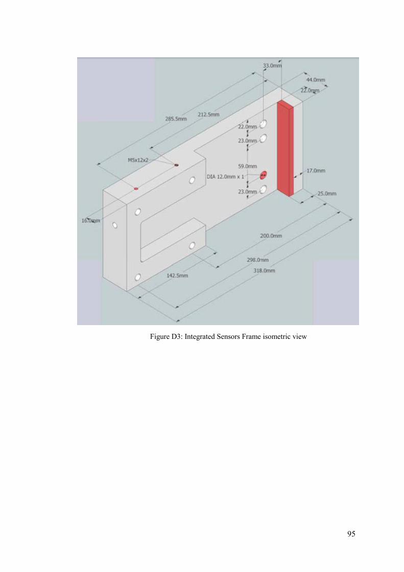
95
Figure D3: Integrated Sensors Frame isometric view
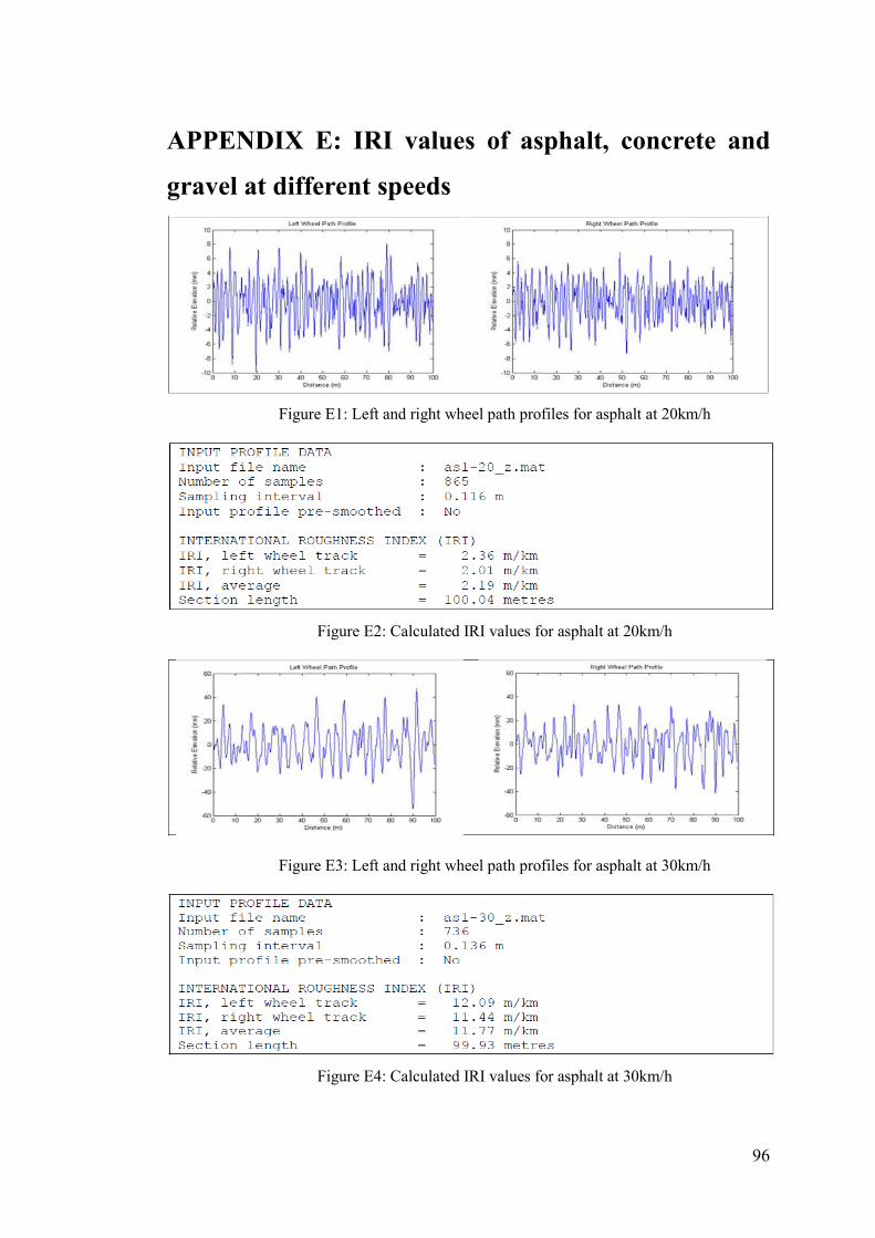
96
APPENDIX E: IRI values of asphalt, concrete and
gravel at different speeds
Figure E1: Left and right wheel path profiles for asphalt at 20km/h
Figure E2: Calculated IRI values for asphalt at 20km/h
Figure E3: Left and right wheel path profiles for asphalt at 30km/h
Figure E4: Calculated IRI values for asphalt at 30km/h

97
Figure E5: Left and right wheel path profiles for asphalt at 40km/h
Figure E6: Calculated IRI values for asphalt at 40km/h
Figure E7: Left and right wheel path profiles for concrete at 30km/h
Figure E8: Calculated IRI values for concrete at 30km/h

98
Figure E9: Left and right wheel path profiles for concrete at 40km/h
Figure E10: Calculated IRI values for concrete at 40km/h
Figure E11: Left and right wheel path profiles for gravel at 20km/h
Figure E12: Calculated IRI values for gravel at 20km/h
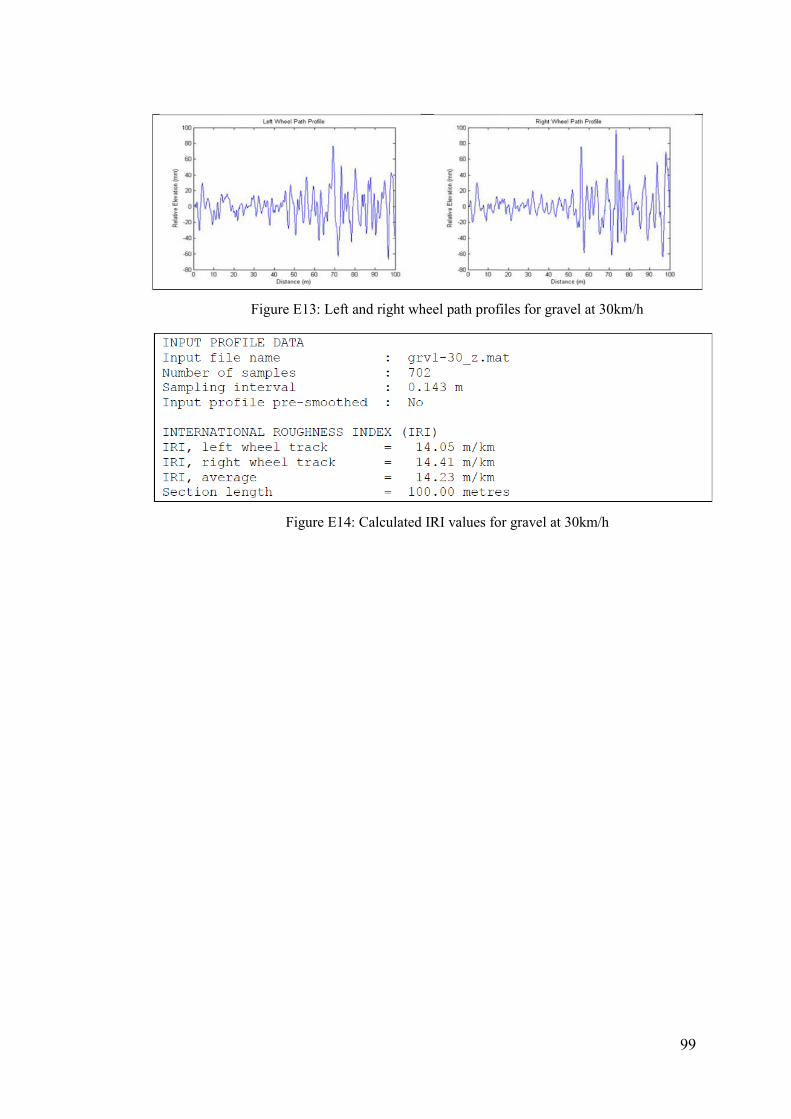
99
Figure E13: Left and right wheel path profiles for gravel at 30km/h
Figure E14: Calculated IRI values for gravel at 30km/h

100
Curriculum Vitae
Xiang Luo
89A Mooramie Ave., Kensingtion, NSW, 2033 Phone: 0411 708 604 | [email protected] Australian
Personal Objective
After four years of undergraduate study and two years of postgraduate research experience, I am seeking a meaningful and challenging position in the engineering industry that enables me to learn new skills and allows for advancement. Education
The University of Technology, Sydney (UTS) Sydney, New South Wales Master of Engineering (Research) 2011- 2013 Thesis topic: Real Time Exteroceptive Sensor Data Acquistion and Processing for an Autonomous System Faculty of Engineering & Information Technology The University of Adelaide Adelaide, South Australia Bachelor of Engineering (Electrical & Electronic) Honors 2006 - 2010 School of Electrical and Electronic Engineering Leadership
Co-director of Integrated Navigation and Automatic Survey Team,
ARC Centre of Excellence for Autonomous Systems, UTS 2011-2012
Professional Work Experience
Vacation Student - Electrical Engineer, Xi’an, P.R. China Qian-Shan Avionics Pty Ltd 2009-2010 Initiated, planned and delivered engineering projects under my scope Managed and maintained effective working relationship with suppliers and
contractors Selected Project Experience:
o Eagle-500 light aircraft Primary Flight Display (PFD) design Studied and interpreted Federal Aviation Administration (FAA)

101
airworthiness directives (DAs) for electrical power, antenna and internal wiring.
Participated in the EDA design on the power module. o Cockpit Voice Recorder (CVR) upgrade
Added video recording function of CVR; Image and speech processing were used to perform video compression.
o Flight Data Recorder (FDR) solid memory module Light-weight tasks were assigned, such as drafting assistance and
checking production progress with dispatcher;
Research Experience & Professional Development
The University of Technology, Sydney ARC Centre of Excellence for Autonomous Systems Projects: 2011-
2012
Automatic Road Clearance Surveying (ARCS) o System design; o Hardware testing, sensors connection (laser sensors, inertial sensors); o System testing, data acquisition and electrical installation. o Data collection and processing;
Pedestrian Dead Reckoning Navigation with Zero Velocity Update 2012-2013 o Sensors selection, hardware testing for the inertial sensors; o Data collection and processing;
Faculty of Engineering
Teaching Assistant 2012-2013
o Tutor of Introduction to Mechanical and Mechatronic Engineering; o Teaching assistant/field work of Surveying;
Publications & Presentations
Automatic Road Clearance Surveying with Sensor Fusion, paper proceeding to the Australian Conference on Robotics and Automation (ACRA), Monash University, 2011.
DEC/2011
Mobile Surveying System for Road Assets monitoring and Management, paper proceeding to IEEE Conference on Industrial Electronics and Applications (ICIEA 2012).
Automatic Road Surface Profiling with Sensors Fusion
Paper proceeding to 12th International Conference on
NOV/2011

102
Control, Automation, Robotics and Vision (ICARCV 2012) DEC/2012
Presenter of Paper “Automatic Road Surface Profiling with Sensor Fusion”
DEC/2012
Professional Skills
Engineering Software: AutoCAD, SolidWorks, Altium, PSpice and MATLAB (Proficient);
Programming Skills: JAVA, C/C++;
General Skills & Interests
Language: Fluent in Mandarin Chinese and English;
Driving Skills: Australian Provisional license
Interests: Basketball, Badminton, Volleyball, Table-Tennis, Documentary Movies
Referees available upon request