ream guidelines for road drainage design - volume 3
TRANSCRIPT


FOREWORD
Road Engineering Association of Malaysia (REAM), through the cooperation andsupport of various road authorities and engineering institutioni in Muluys'ia, publishesa series of official documenrs on sTANDARDS, spgcm,tcATloNs, GUIDELINES,MANUAL and TECHNICAL NOTES which are related to road engineering. Theaim of such pubiication is to achieve quality and consistency in road and highwayconstruction, operation and maintenance.
The cooperating bodies are:-
Public Works Deparrment Malaysia (pWD)Malaysian Highway Authority (MHA)Department of Irrigation & Drainage (DID)The Institution of Engineers Malaysia (IEM)The Institution of Highways & Transportation (IHT Malaysian Branch)
The production of such documents is carried through several stages. At the Forum onTechnology and Road Management organizeo uy rwuREAM in Novemb er 1997,Technical Committee 6 - Drainage was formed with the intention to review ArahanTeknik (Jalan) 15/97 - INTERMEDIATE GUIDE To DMINAGE DESIGN oFROADS' Members of the committee were drawn from various goue**"ntdepartments and agencies, and from the private sector including privitized roadoperators, engineering consultants and drainage products minufacturers andcontactors.
Technical Committee 6 was divided into three sub-committees to review ArahanTeknik (Jalan) l5l9l and subsequentry produced 'GUIDELINES FoR ROADDRAINAGE DESIGN' consisting of the folrowing vorumes:
Volume 1 - Hydrological AnalysisVolume 2 - Hydraulic Design of CulvertsVolume 3 - Hydraulic Considerations in Bridge DesignVolume 4 - Surface DrainaseVolume 5 - Subsoil Drainale
The drafts of all documents were presented at workshops during the Fourth and FifthMalaysian Road Conferences held in 2000 and,2002 respectively. rfr" comments andsuggestions received from the workshop participant, *"r" reviewed and incorporatedin the finalized documents.
ROAD ENGINEERING ASSOCIATION OF MALAYSIA46-A, Jalan Bola Tampar r3/r4, Section 13, 40100 Shah Alam, Selangor, Malaysia
Tel: 603-5513 652r Fax: 5513 6523 e-mail: [email protected]

iiI
TABLE OF CONTENTS
Page
3.' INTRODUCTION ...3-7
3.2 PRELIMINARY INVESTIGATION ........3-i3.2.7 Site Selection ... "....3-13.2.2 Reconnaissance Survey ..... ......3-z3.2.3 Data Collection . ......3-3
3.3 SURVEY DATA ...,..3-43.3.1 Survey of Bridge Site and Beyond ......3-43.3.2 Hydraulic Survey .....3-6
3.4 ESTIMATION OF DESIGN DISCHARGE AND WATER PROFII,E ...3-53.4.I Design Recurrence Interval ........3-63.4.2 DesignDischarge ...,.3-"13.4.3 Water Profile ...3-8
3.s BRTDGE WATERWAY . . .........3-9
3.6 SCOUR AT BRIDGE CROSSING . ....3-93.6.1 Scour .....3-93.6.2 Countermeasures .....3-11
3.7 FORCES ON BRIDGE PIERS ...3.1]
3.8 DESIGN OF BRIDGE TO ALLOW FOR FUTURERIVER IMPROVEMENT WORK ,....3-17
LIST OF FIGURES
Figure 3.1 Extent of Survey for Bridge Site .. ......3-5Figure 3.2 Scour at a Bridge Site . . .....3-10Figure 3.3A Typical Wire Enclosed Riprap ....3-I2Figure 3.38 Typical Interlocking Concrete Block and Cable Tied Block System ..3-73Figure 3.3C Typical Articulated Grout Filled Mat Design .......3-I4Figure 3.3D Typical Cement/Grout Filled Bags at Abutment . "..3-15Figure 3.3E Typical Cement/Grout Filled Bags at Pier .. ....,.....3-16Figure 3.4 Freeboard and Embedding Depth for Footing ........3-19

LIST OF TABLES
Table 3'1 Recommended Average Recurrence Interval for Design Discharge...3-7
LIST OF REFERENCES ...,.....3-20
APPENDIX 1Reprint of Appendix D - Hydrauiic Design of Bridges, Urban Drainage Design Standards AndProcedures For Peninsular Malaysia No. I (1g75).

VOI-UME 3 - HYDR.AULIC CONSIDER.ATIONS NN BR.IDGE DESIGN
3.1" INTR.ODUCTION
The design of a bridge over a waterway requires a comprehensive engineering
approach that not only includes route location, traffic flow forecast and structural
and foundation requirements, but also the assessment of the characteristics of the
river flowing beneath. For this, it is necessary to collect data, and to understand
the factors that govern stream runoff and water surface levels, sediment discharge
and deposition, scour and channel stability and hydrodynamic forces acting on the
bridge" Predictions about likely event under particular site conditions have to be
made.
This volume does not describe in detail ali the factors that require to be
considered in bridge designs, but merely identifies the hydraulic aspects that
characterise a river and provides directions to relevant literature, which give in-
depth details on these aspects. For hydraulic design of bridges, the designer could
refer to Appendix 1 which is extracted from Jabatan Pengairan dan Saliran
publication - Planning and Design Procedure No. 1: Urban Drainage Design
Standards and Procedures for Peninsular Malaysia (1915). The designer is
encouraged to refer to the other relevant literature listed in the References.
PRELIMINARY INVESTIGATION
Site Selection
Ideally the cost of alternative river crossing locations should be considered when
making the preliminary selection of a route. However, in built-up areas the site
for a bridge and the approach roads are usually fixed and dictated by the town
layout plan.
In rural areas, the bridge crossing is restricted to certain reaches of the river owing
to constraints imposed by existing landuse, road alignment and the river
meanders. The selection of sites has to be made within these reaches and should
avoid costly river works and land acquisitions.
3.2.
3.2. r
3-r

Fs
F
F!.
3.2.2
Bridge site selection normally commences with a desk-top study of availabletopographic maps which detail the geomorphologic features of the surroundingland, landuse, river pattern, meanders, sand deposits and sometimes, bank levels.on these topographic maps several potential bridge sites may be identified.
The choice of a crossing site will be governed primarily by the main channelwidth and the proportion of overbank flow to total flow. Logically, the firstconsideration should be given to those sites that have the narrowest main channeisand the smallest proportion of flood plain flow.
On wide flood plains where rivers tend to meander, first consideration should begiven to crossing sites where the channel could be controlled with minimal rivertraining works. Occasionally rock outcrop or inerodible bank material may belocated to reduce the requirement of river trainins works.
Other possible sites are at crossover modal points in the river meander patternwhere the channel is wider and shallower and at bends where the channel isnormally narrower and deeper particularly at the outside of the bend. Theoptimum location should be decided by considering the channel geometry, bankstability, river training work and type of bridge construction.
The desktop study should also include a literature search and examination ofrecords or reports on river improvement works completed or yet to beimpiemented by Jabatan Saliran dan Pengairan (JPS) and other sovernmentagencies.
Reconnaissance Survey
Bridge sites desktop study will include reconnaissance survey with theto gain a general appreciation of the river behaviour by examiningrecords and by carrying out field inspections. Information on theshould be collected:
(b)
(c)
objective
available
following
(a) river channel regime to determine whether the river has a wide flood plain.or whether it is incised with little or no flood piain.
river channel stability to determine whether the river is stable or unstable.
river channel flow pattern, if it is sinuous, determine whether the channelmigration is active,
J-L

.
(d) range of water levels, particularly high-water levels and their frequency of :
occurrence, historical flood events could be indicated by riverine users or
local inhabitants.
(e) range of discharges, particularly for floods and their frequency,
(f) width of waterway, width of flood p1ain, meander length and width,
(g) type and grading of river bed materials,
(h) type of material composing the river banks,
(i) iocation of any naturai outcrops of inerodibie rock which may restrict
channel movement. and
C) extent of any regional floods in the locality.
Some of the above information may be obtained from topographic maps, aerial
photographs, JPS hydrological records, previous river basin or drainage study
reports and existing and proposed future river improvement works.
The preliminary study of the bridge sites should include an estimation of the river
flood flows by current acceptable hydroiogical procedures, if stream flow records
at the selected sites are not available.
3.2.3 Data Collection
Other information could be obtained by field inspection such as:
(a) type and grading of river bed material,
(b) existence of shoals and their composition,
(c) the material forming the river bank,
(d) vegetation on the bank,
(e) steepness ofbanks and evidence ofbank erosion,
(f) erosion pockets in the bank,
(g) existence of inerodible rock,
(h) debris marks on shrubs, trees or banks which may indicate the water level
of recent floods.
3-3

'I
: (t
0)
watermarks on walls, jetties and piers and buildings which indicate recenthigh water levels and
conskiction to water flow.
3.3.
3.3.1
When the assessment of the survey information has beensite for a bridge crossing from the fluvial aspect may befield surveys of the site will then follow.
SURVEY DATA
Survey of Bridge Site and Beyond
Spot levels within the survey corridor shall beinterval and shall include the bank levels and thebottom of the banks, centre and deepest points.
compieted, acceptable
chosen. The detailed
taken at not more than 10 minvert levels of the river at the
I
I
t
It!.
t:_tIII
After the selection of suitable sites for the bridge crossing have been made,hydrographic and hydraulic surveys have to be carried out to obtain the datarequired to determine the width of the bridge opening, the depth of scour andhydrodynamic forces on piers and the upstream backwater.
For large and deep rivers the hydrographic survey should be carried out by usingrecording echo sounder systems. The topographic features of the river and floodplain on both banks should also be surveyed by normal topographic surveyprocedures, to the extent required for hydraulic analysis.
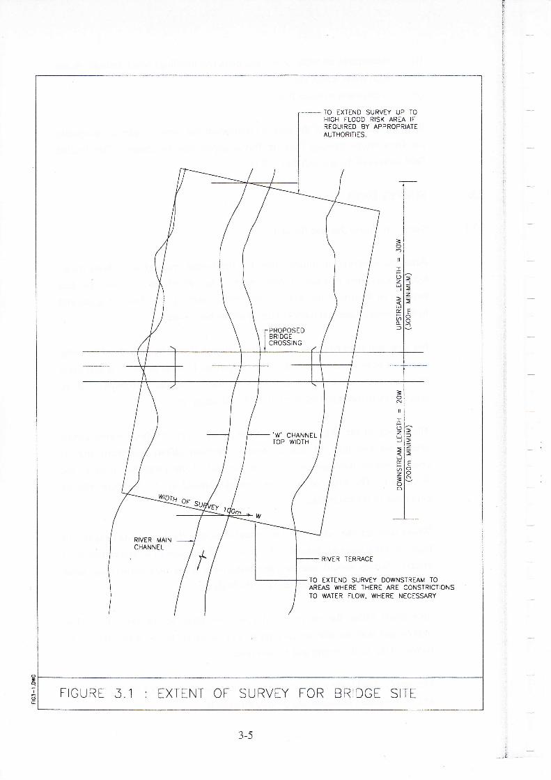
The survey of the alignment and contour of the river and flood plains shouldextend not less than 30 channel widths upstream (300m minimum) and, 20channel widths downstream (200 m minimum) of the proposed crossing, seeFigure 3'1' The width of the survey corridor should not be less than 50m oneither side of the riverbanks.
where required, the survey shall be extended beyond the bridge site to upstreamhigh flood risk areas to obtain data for analysis of backwater and assessment of itseffects" Survey should also include downstream water flow constriction areaswhere they may affect the hydraulics of the bridee.
The survey should also include taking of panoramic photographs of the bridge siteand its immediate upstream and downstream reaches.
3-4
gFi:
TO EXTEND SURVEY UP TOHIGH FLOOD RISK AREA IFREOUIRED BY APPROPRIATEAUTHORITIES.
Itsz)
u.Fao-
l
=
oon
RIVER MAINCHANNEL
RIVER TERRACE
TO EXTEND SURVEY DOWNSTREAM TOAREAS WHERE THERE ARE CONSTRICTIONSTO WATER FLOW. WHERE NECESSARY
SURVIY FOR
.W'CHANNEL
TOP WIDTH
FIGURI 3.1 : tXTINT OF BRIDGI SITt
3-5
s

3.3.2
The hydrographic and topographic surveys should be plotted on the same plan tofacilitate extraction of cross-sectional data for hydraulic analysis and all levelsshould be reduced to a common datum.
For scour analysis samples of the riverbed materialsize analysis at the crossing and upstream locations.
Hydraulic Survey
should be taken for particle
For large rivers the discharge passing through the proposed bridge site should bemeasured at a number of different stages of flow. Each discharge measurementshould be related to the date of survey, time and water levei and be reciuced to astandard datum. A gauging station should be established near the site of theproposed crossing as soon as possible.
Velocities of flow in both magnitude and direction (in tidal sites) should bemeasured across the river channel, preferably, during high flows and could be partof the discharge measurement prograrnme.
The designer should check with JPS stream flow records whether the river in thevicinity of the proposed bridge site has been gauged. Any information availableshould be incorporated in the hydrological study.
ESTIMATION OF DESIGN DISCHARGE AND WATER PROFILE
Design Recurrence Interval
Stream flows for the 2,5, r0,25,50 and 100 years average recurrence intervals(ARI) should be derermined.
The ARI of the design discharge should be in accordance to Table 3.r.Nevertheless, factors such as possible loss of life and economic damages due toany failure, have to be set against the higher capital cost of a bridge designed for alonger ARI must be considered.
3.4.
J.+. I
3-6

Table 3.1: Recommended Average Recurrence Interval for Design Discharge
Type of Structure
Averase Recurrence Interval in Years
U2IF(2and lower
u3 -u4/R3-R4
u5 - u6lR5_R6
Bridge 50
25*
100
50x
100**
100*
Note:*The above average recuffence intervals can be used by the designer ifany of the following conditions applies:
a) the structure is located in a flood plain
b) the structure requires a high embankment
c) the soil condition is poor making high embankment construction
uneconomical
Under the above conditions, the structure must be designed as a submersible
structure. Special consideration, however, must be given against accumulation
of debris o, i*p^"t by floating logs etc.
** For major bridges, the probability of the design flood being exceeded
should not be more than 57o tn the design life
3.4.2 Design Discharge
Design discharge at the proposed bridge site can be determined in accordance
with the various flood flow estimation hydrological procedures published by JPS.
Where stream flow records are available for a particular station in the river or
located near to the proposed crossing, then the more accurate method of
streamflow frequency analysis should be adopted.
In the estimation of the design discharge, an assessment of the extent of current
and future landuse development in the catchment has to be made and corrective
measures must to be included in the estimated discharge if future landuse changes
are going to be significant.
It would be useful to indicate on bridge drawings the estimated discharge and
water levels of the river for various recuffence intervals. This information can be
used as a guide in the planning and design of temporary works at the bridge site.
3-7
E

3.4.3 Water Profile
Where water level records are available at the crossing site, a frequency analysisshould be carried out, otherwise, the water level corresponding to the designdischarge can be calculated by a suitable flow equation, such as Manningformula. Where river stage discharge charts are available, water levels forvarious flows may be read off the charts.
For wide rivers, it is usually uneconomical to construct a bridge with a singlespan' More often multiple piers wiil be provided within the flood flow channeland earth embankments will encroach into the flood plain. These will constrictthe flow and cause upstream water levels to rise above the original free flow level.
The amount by which the water level rises above the freecalculated by the method described in the sub-sectionBackwater in Appendix 1.
fiow level, may be
on Computation of
Should there be numerous river cross-sections and design flood flow scenariosthen the manual calculation method cited in the foregoing will become timeconsuming. Many affordable water profile analysis software are now available tothe designer to perform the task, such as:
o HEC 2 - Water Surface profiles
o WSPRO (HY-7) - Bridge Waterway Analysis Modelo HEC-RAS : River Analysis Svstem
The above are obtainable from Hydrological Engineering center, uS Army corpsof Engineers and are very versatiie and capable of handring:
o
o
o
o
o
o
eccentric location of main channel within the flood plainskewed orientation of bridge crossing
various pier shapes and spacing
discharge through partially submerged bridgesdischarge over submerged road embankments andscour at pier and abutment.
3-8

?{ BRIDGE WATER.WAY
The bridge waterlvay area to be provided should be sufficient to ensure the design
flood can safely pass through without undue afflux or excessive increase in
upstream flood levels, and at a velocity, which will not increase scour to such an
extent, as to endanger the stability of the bridge structure.
Sufficient clearance of bridge deck above flood levels should be provided to
allow the largest floating debris to pass through without clogging up the
waterway. The minimum amount of freeboard is 1.0m above the design high
water level. Where the river is navigable by watercrafts attention should be given
to the headroom clearance required by the controlling authorities. When it is
necessary to restrict the width of the waterway to such an extent that the scour
would be severe, protection against damage shouid be made by providing deep
foundations and adopting appropriate scour counter-measures.
Where there is existing drainage or irrigation dikes aiong the banks of the rivet,
the soffit of the bridge deck and beams should be placed a minimum of 0.5m
above the top of these dikes. The freeboard between the high water level and the
top of the dike is usually 0.5m to 1.5m depending on the design discharge of the
river, however this needs to be checked with the appropriate river authorities,
mainly JPS.
SCOUR AT BRIDGE CROSSING
Scour
Scour can be very insidious whereby soil around a bridge foundation is removed
and re-deposited elsewhere during a flood. The most common form of flood
damage to bridges arises from the scouring of abutments and piers, which can
underinine the structure, resulting in collapse of spans and possible loss of life.
Four different types of scour must be considered, as follows:
General Scour
General scour is the depth to which
scoured below the natural bed ievel.
constriction of flood flows through the
or embankments (see Figure 3.2).
the riverbed at the bridge site is
This normally occurs due to the
bridge opening between abutments
3.6
3.6.1
a)
3-9
7
I
I
I
I-l
.l
I
II

L!F
Ldr\CMm
F
M-lr\
Nfrr^)
n\l_f
t-,--
LLllOI/-\ I
-l-JfYlmi-1*l\rl--)/-tvl"l-rlFl
I
zlct'lf-l(JlLrJlal
ul
U)
I.Fto-lr trJI - |
KJ-n#,/J 5Et C) UJIJJ Lr) COZrLLI I9i.l
T_J_J
L
J l,l^=(J4-o-;F
ti'^-/-i --1 -r-;/lvl
'r I
n--l
Jt!
E.o_
ozf
J
zE
m
zLrJ
Ffco
YOUc)trl
oEm
ztrJ
F:)cE)
,l,lI'o
ru<cD1noa>OE
3-10
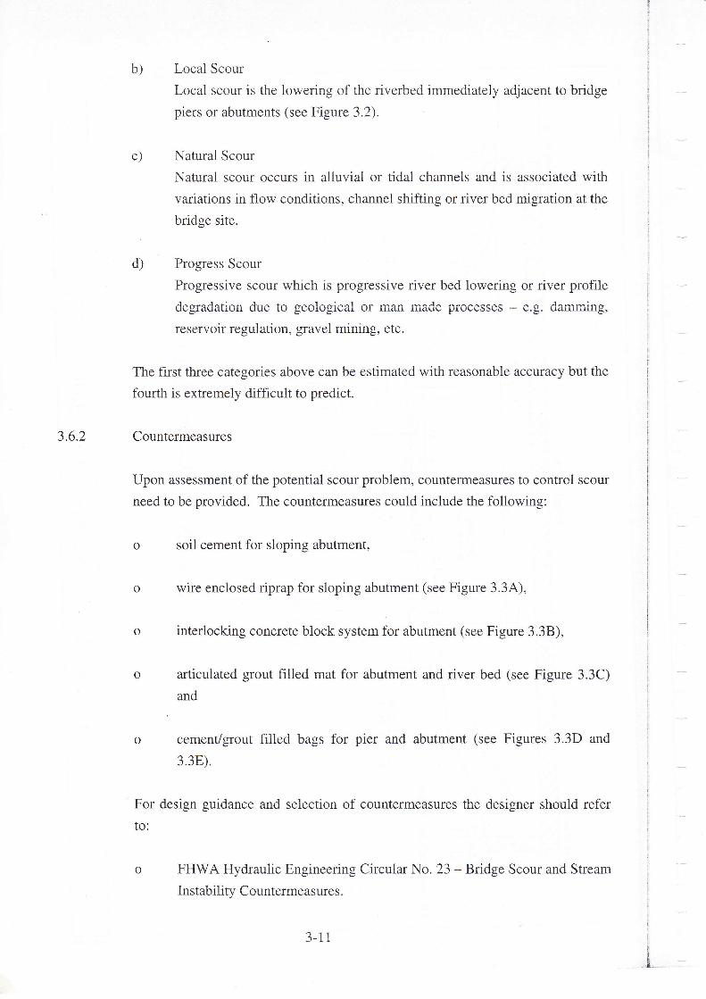
b) Local Scour
Local scour is the lowering of the riverbed immediately adjacent to bridge
piers or abutments (see Figure 3.2).
c) Natural Scour
Natural scour occurs in alluvial or tidal channels and is associated with
variations in flow conditions, channel shifting or river bed migration at the
bridge site.
d) Progress Scour
Progressive scour which is progressive river bed lowering or river profile
degradation due to geological or man made processes - e.g. damming,
reservoir regulation, gravel mining, etc.
The first three categories above can be estimated with reasonable accuracy but the
fourth is extremely difficult to predict.
3.6.2 Countermeasures
Upon assessment of the potential scour problem, countermeasures to control scour
need to be provided. The countermeasures could include the following:
o soil cement for sloping abutment,
o wire enclosed riprap for sloping abutment (see Figure 3.3A),
o interlocking concrete block system for abutment (see Figure 3.3B).
o articulated grout filled mat for abutment and river bed (see Figure 3.3C)
and
o cement/grout filled bags for pier and abutment (see Figures 3.3D and
3.3E).
For design guidance and selection of countermeasures the designer should refer
to:
o FHWA Hydraulic Engineering Circular No. 23 -Bridge Scour and Stream
Instability Countermeasures.
J-IIi,,

o_
C(o_M
tlLl-jaJ
Z-L!
L!a_
=--J
o-
F
N-)
()l_f
L-
LLJI
OI-l-lrvl.nl-l
Irlr\l\JI
-lI
-lclC\./ I,,1rl-lzla)l,lf-l()lLJ.ll(^l
r--r-_- --==1I L----I L-----.-i f---*--J
r--j**--;-,
azm
t
=oUF
o
LiJ)FxtrlF
LrJ
zLd
=Izz
U(Y ITJtr)Fii
o_
o7--2 =E
-JJ
z,-itr
O
".2()oaF
o->
N
c
c0
FzFlCD
)<
L!c)
ae.co
FzLJ
Flcn
zm
1
F
oz)e
zaXt!
v.F
3-12

l4
i--
-Z
)<
--Jm
L!FLr-J
E.O21 lr-)Or-";19 /)ZwY9!2oL)JI arltLl r-rFii7=
rl'l<:lOmn<>rJF
mtt-)
nL!t_lt-r-
I
I
II
E.
-zozft
II
zFF
)<
rt JzuV u-rC)F9HLrzFA. 26
CIELE.DIYG
3-13

ZrlaLLiOF
OIllI
I
IFlMrl
OLIF-_Jl
Fa__J
r)o-
F
rlM)
t')
()
lC}
Lr-
z,l1tn-l-l
ozHoi;>z:r.
>IOCJU.Zo-<
TIrl<t
Izlvl,l-lHIal
FE.
zOun7*^o vuii a>;:i
d)a@zof6+
oz
I'!J?:>L<)<x<L! CO
III\
oU0a
Th()0.-j CSAZ<UL! (J
oco
J
zzI
)-lz,UI'lUIc)l-E(D
-JJ__J
J-1J
-J-J-JJJ)J-Fz
Fl
3-r4 FIGJ-3C.DWG

EMBANKMENT
EXISTINC STREAMBOTTOM
NON-WOVEN GEOTEXTILT FILTER *"u*-.J ABUTMENTFOOTING
SECIION THROUGH ABUTlvlINT
NOTE :
(r) DO NOT EXCAVATE BELOW BOTTOM OF FOOTINGTO ACCOMMODATE CONCRETE BAGS
THE N AREA DENOTES PORTION OF
STREAM,BOTTOM TO BE EXCAVATED TO
ACCOMODATE CONCRETE BAGS
\1)
FIGJ-30 DWG
FIGURE 3.3D TYPICAL CEMENT/GROUT FILLID BAGS AT ABUTMENT
3-15
f-
T
1
I
I
I
I
II
I
IItt.L

E.[Jo-
F
m
OIrl
--JLL
FlE.a\
Z.lrl
Ll-J(J
J
r\o-
F
LJ
l..j
Ll-Jul
I
z?0.P9?I RinP XXZ LLJ t4)Lrl mFA _tJ
<:c)UZg >P- ovs Eu.rN\ FN 6*K\XN >=hJ <<l,J G()F (r<
-lFI
zl
ftlL!lnl-l Irl-lJl-\lvlrYl-rl
=lIIzl
a-\lvl;-l-l(JlL!l6l
U
o
O
F
zU>nFV,,!dF r,r<=> :\,.iZxO
LJ
FU7
2=Fl"
=FxoLrJ Ct)
zUFxUJFx,^a)<
U)>ail<50_9ezoOOz{)
Utd)E.UF
=
Ec\J
E
q
EN
or
,4
)<
LrJOL!rtQtco
IIl
I
I
i
I
.-J..
3-16

3.7
Sub-section 29.2 - Erosion and Scour Protection, Urban Stormwater
Management Manual for Malaysia.
FORCES ON BRIDGE PIER.S
Piers in the flow path are subject to the following forces.
o hydrodynamic forces
o floating debris forces
o water-craft coiiision impact forces
Accumulation and clogging of d,ebris upstream of the bridge can cause a majcr
build-up of horizontal destabilising forces owing to the damming effect. To
design the struciure io resist this effect may not be economicai and may be
cheaper to provide a larger freeboard.
Where the river is navigable, piers within the waterline shouid be <iesigneii
against possible collision by watercraft.
3.8 DESIGN OF BRIDGE TO ALLOW FOR FUTURE RIVERIMPROVEMENT WORK
To allow for future river deepening work, (see Figure 3.4'), the embedding depths
for bridge footings and pilecaps shall be as follows:
Item Location of Pier Embeddine Depth
i) Low water channel and the part ofhigh water channel within 20m
from the top of the slope of low
water channel.
For footing - more than2mbelow
the river bed of low water channel
For pilecap - I.Zmbelow bed oflow water channel
ii) High water channel beyond 20m
from the top of the slope of low
water channel
For footing - more than 1m below
the river bed of high water channel
For pilecap - 1m below river bed
of hieh water channel
The top of foundations in the 1ow water channel should also be below the level ofthe estimated totai scour depth when the total scour depth is below the designed
invert level of the future river deepening work.
3-r7

On major road where slow-moving maintenance equipment are not permitted tooperate on the roads and where space is available, 5 to g m wide berms, with 3.5mheadroom, near the river channel shouid be provided to facilitate movement ofriver maintenance machinery, as shown on Figure 3.4. The river channel at thebridge should be shaped to accommodate the future river channel improvementworks and temporary riverbed erosion scour counter-measures should be providedto reduce degradation of upstream river profiles.
3-1 8

t
:rF
Ua
E
.
ts(L
tlzood)
N
I&o
zoU
E
N
E
a
';
I
o
*>Z
)UzzI
x.F
=I
=
)Uzz=v.
==)
)Uzz
'I
EUF
=T
=
@
FzU
Flm
r\Z.F-)LL
M-
L-r--
IFo_LdOr\Z.=flOttlCO
ttt
cZ
OU-
COLLJLlJMLr-
<.-
Ir/-)
c)l_lC'')
L
t
I
dIoz
()-0
E)
5aegj
EoI
€q
otE@
noO
=UzzFza
ot&&
o(D
u
e.
ElF
FztrJ
Ffm
G
-I
-
3-r9

LGCAL PUBI,ICATIONS
l.
LTST GF REFER.ENCES
Hydrological procedure No. 4- Magnitude and Frequency of Froods in peninsurar Malaysia (19g7)
Hydrological procedure No. 10
- Stage Discharge Curves (1916)
Hydrological Procedure No. 11
- Design Flood Hydrograph Estimation for Rural Catchments in peninsularMalaysia
Hydrological procedure No. 19
- The Determination of suspended Sediment Discharse
Hydrological procedure No" 5- Rational Method of Frood Estimation for Rurar catchments
Hydrological Procedure No. 1
- Estimation of the Design Rainstorm in peninsurar Malaysi a (r9gz)
Hydrological procedure No. 16
- Flood Estimation for Urban Areas in peninsular Malaysia
Planning and Design procedure No. 1
- urban Drainage Design standards and procedures for peninsurar Maraysia
Garispaduan untuk Memproses permohonan dan Menetapkan Syarat-syarat BagiJambatan dan Lintasan
Urban Stormwater Management Manual for Malaysia
Draft Intermediate Guide to Drainage Design of Roads- Arahan Teknik (Jalan) 15/gl
Terms of Reference for survey works and Digital Ground Modellins.
3-20
2.
3.
n+.
10.
11.
5.
6.
8.
9.
I
,:.*
12.
abatan Keria Raya (JKR

It.
2.
3.
4.
US PUBI,ICATIONS
Hydraulic Design Series No. 2
- Highway Hydrology (Sept 1996)
FHWA-SA-96-061
Hydraulic Engineering Circular No. 22
- Urban Drainage Design Manual (Nov. 1996)
FHWA-SA-96-078
(us DoT FHA)
Hydraulic Engineering Circular No. 14
- Hydraulic Design of Energy Dissipators for Culverts and Channels
(Sept. 1983)
(us DoT FHA)
Hydraulic Design Series No. 5
- Hydraulic Design of Highway Culverts (Sept. 1985)
FHWA-IP-85-15
(us DoT FHA)
3-2r

APPENDIX 1
X{YDRAULIC DESIGI\ OF' BRIDGES
This appendix is an exact reproduction of Appendix D - F{ydraulicDesign of Bridges as found in Jps planning and Design procedureNo. 1 _ URBAN DRAINAGE DESIGN STANDARDS ANDPROCEDURES FOR PENINSULAR MALAYSIA ( 1975).
The permission granted by JPS to REAM to publish the whole of theabove appendix in gratefully acknowledged.
REAM

pressnts some bridge design criteria, describes the genefal flow conditionsbridge design, the computation of backwater and some design exampres. For apresentation, the reader is referred to the excellent pubtication by the u.s.Transportation, Hydrauric Design series No. 1, ,,Hydraulics of Br:idge water-
Dl.1 Design Criteria
Bridge openings shoufd be designed to hane as little effect on the flow characteristics as ispossible' consistent with good bridge design and economics. In regard to supercriticalflorr witha lined channel, the bridge should not affect the f low'at all. That is, there shoutd be noprojections into the design waterway.
Dl.z Design Approach
The method of planning for bridge openings must include vrrater surfece profile and i.lydreullcgradient analyses of the channel for the major storm runoff. Once this hydrautic gradient isctablished without the bridge, the maximum reasonable effect on the channel flow by thebridge should be determined. Generally in urban cases this shourd not exceed a backwatereffect of more than 6 to 12 irnhes
Velocities through the bridge and downstream of the bridge must receive consideration inchoosing the bridge opening. velocities exceeding those permissible will require specialprotection of the bottom and banks.
For supercritical f low, the clear bridge opening should permit the flow ro pass under unimpededand unchanged in cross section.
D1.3 Bridge Opening Freeboard
The distance between the design flow water surface and the bottom of the bridge deck willvary from case to case. However, the debris which r.v u, expectd must receive full consi-deration in setting the freeboard. Freeboard may vary from several feet to minus several feet.There are no general hard and fast rules. Each case,rit b" studied separately.
Bridges which are securely anchored to foundations and designed to withstand the dynamicforces of the flowing water, might in some cases be designed without freeboard.
In certain unusual cases, the designer might properly choose to intentionally cause pondingupstream from bridges to reduce downstreim peaks during the storms creating flow greater thanthe initial design runoff. This is sometimes done when d;wnstream areas are highty developed,and the upstream areas have adiacent open pace and park areas next to the channel. In thesecases' there normally would be no freeboard allowed between the design water surface and thebridge deck bottom.
Dl. GENERAL
This Appendixencountered inmore completeDepartment ofways".
i
I
I
I
i
-.:g
97
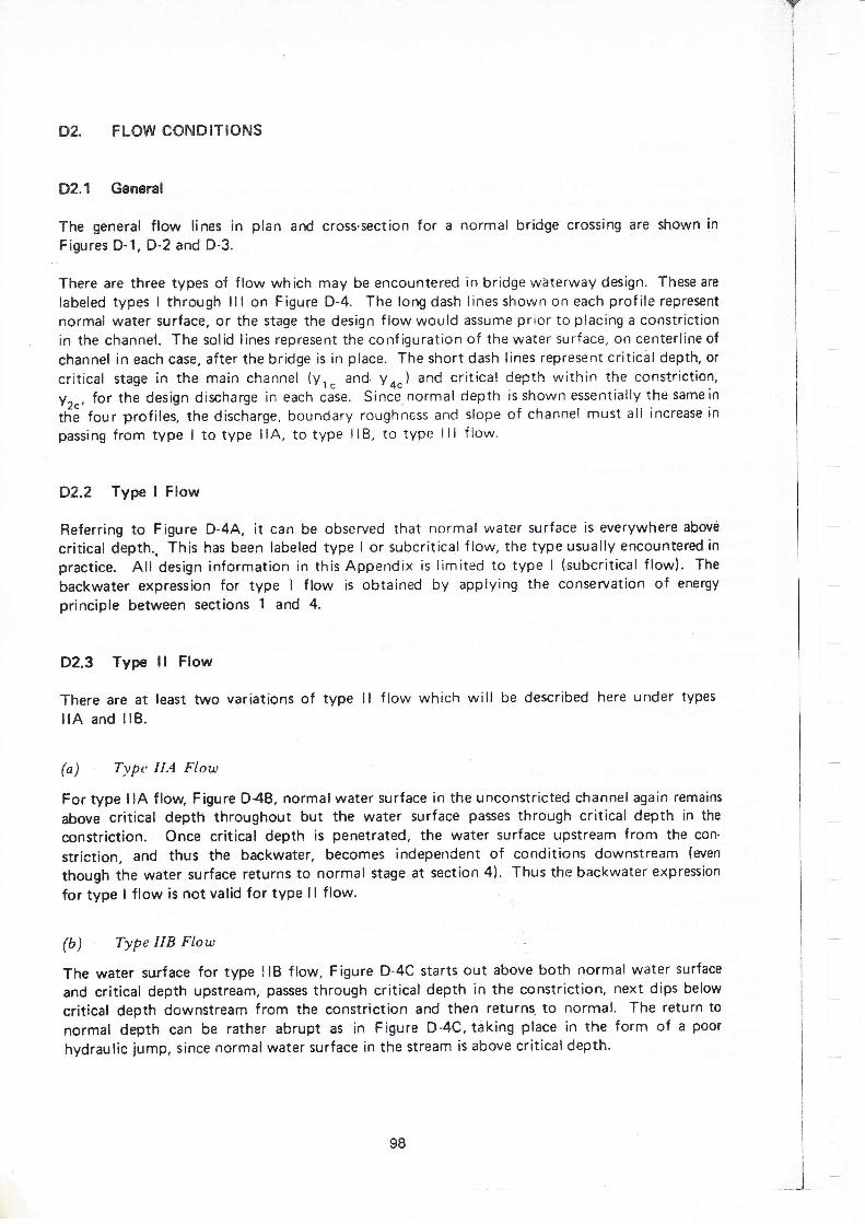
D2. FLOW CONDITIONS
D2.1 General
The general flow lines in plan and cross-section for a normal bridge crossing are shown in
Figures D-1, D-2 and D-3.
There are three types of flow which may be encountered in bridge waterway design. These are
labeled types I through lll on Figure D-4. The long dash lines shown on each prof ile represent
normal water surface, or the stage the design flow would assume prior to placing a constrictionin the channel. The solid lines represent the conf iguration of the water surface, on centerline of
channel in each case, after the bridge is in place. The short dash lines represent critical depth, or
critical stage in the main channel (V.," and. vo") and critical depth within the constriction,y2", tor the design discharge in each case. Since.normal depth is shown essentially the samein
tli6 four profiles, the discharge, boundary roughness and slope of channel must all increase in
passing from tvpe I to type llA, to type llB. to type lll flow.
D2.2 Type I Flow
Referring to Figure D-4A, it can be observed that normal water surface is everywhere above
critical depth.. This has been labeled type I or subcritical f iow, the type usually encountered in
practice. All design information in this Appendix is limited to type | (,subcritical flow). The
backwater expression for type I flow is obtained by applying the conservation of energy
principle between sections 1 and 4.
D2.3 Type ll Flow
There are at least two variations of type ll flow which will be described here under types
llA and llB.
(o) Typ( IL4 Flow
For type llA floW Figure D4B, normalwater surface in the unconstricted channel again remains
above critical depth throughout but the water surface passes through critical depth in the
constriction. Once critical depth is penetrated, the water surface Llpstream fronr the con-
striction, and thus the backwater, becomes independent of conditions downstream (even
though the water surface returns to normal stage at section 4). Thus the backwater expression
for type I flow is not valid for type ll flow.
(b) Type IIB Ftow
The water surface for type llB flow, Figure D-4C starts out above both normal water surface
and cr,itical depth upstream, passes through critical depth in the constriction, next dips below
critical depth downstream from the constriction and then returns. to normal. The return to
normal depth can be rather abrupt as in Figure D-4C, taking place in the form of a poor
hydraulic jump, since normal water surface in the stream is above criticaldepth.
98I
II
_ _r__

:-w,1
i
D2-4 Type til Ftow
lntype lll flow, Figure D-4D, the normal water surface is everywhere below criticaldepth andthe flow throughout is supercritical. This is rn ,nrtu.icJsJ requiring a steep gradient but suchconditions do exist, particufarry in mountainous regions. Theoreticaty backwater shourd notoccur for this type, since the flow throughout is supercritical. lt is more than likely that anundulation of the water surface will occur in the vicinity of the constriction, however, asindicated on Figure D-4D.
99

Y!
Qc' 28OO clcw
Qr '8 4 oO clr
Figure D-1.-Flow lines for typical normal crossing.
aIooI
b
ooo elelalo lo
lE ls
a()
ooo
)\| | sEcT.Fr-o
100
iI1
,4,

I
I
3EC?.rh /va\ t/
?,r"'(4)
W.S, TLfuNiJ BATdKgtcr.r^Y
_@! us.-t!
c
I
I.oJlr.
Figure D-2. -Normal crossmg : l{ingutall ab utrnents.
CTUAL tr. S. ON 1lv"
PROFTLE ON STREAM t
sEcTfoN o
PLAN AT BRIDGE
FLOW ----+
W. S. WITH EACKWAT
sEciloN @
101

W. S. ALONG BANK
----
sEcT'toN o
Y
,($
NORTIAL W.S.
s€cT.II
A w.s. oNL
l-- ! "' o'- -i
Q5
bS. WITH EACKWATER
PROFILE ON STREAM O
c*- -:'':-:-.':.-.':.:. -.fl.'.... ...:..:.. .'.:.:.:.:.:.:'"'1.. l.'. I ;.i :.i..:.':,i#
sEcT toN €)
..r.:J- ! !:-
PLAN AT BRIDGE
f igure D-3.-Narm.al crossing: Spillthrough abutments
=oJtr.
lY
t.s. f,tTlr BACKWAIER
102
IT..';{

Y
----Jl,c
---J
r----I
A-TYPE I FLOW (SUSCRTTICAL)
IL_--- cRtTcAL D€PrH
lqc i
f---Irc
.)c ? l,l;-- ----:lryry-- --------jB-TYPE trA FLOIY
( PASSES THROUGH CR|T|CAL)
HYDRAULIC JUMP
I
' t",1,
C-TYPE II8 FLOW( PASSES THROUGH CRTTICAL}
t-- - -€!{aoeerx
D-TYPE III FLOIV(SUPERCRITICAL)
Figure D-4.-Types of flow cncountcred.
--T-::Ff=qY
- tcn,trcat
D€prH
:a
{i.t
103

D3. DEFINIT]ON OF TERMS AND SYMtsOLS
D3.1 Definition of Terms
Specific information is given below with respect .to the concept of several of the terms and
expressions frequently used throughout this Appendix.
(o) Normal Staee
Normal stage is the normal water surface elevation of a stream at a bridge site, for a particulardischarge, prior to constricting the stream (see Figures D-2A, D-3A). The prof ile of the waterslrface is essentially parailel to the bed of the streanr.
(b) Abnormal Stage
Where a bridge site is located upstream from, but relatively close to, the confluence of twostreams, high water in one stream can produce a backwater effect extending for some distanctup the other stream. This can cause the stage at a bridge site to be abnormal, meanirp higher
than would exist for the tributary alone. An abnormal stage may also be caused by a dam,
another bridge, or some other constriction downstream. The water surfaca with abnormal stage
is not parallel to the bed.
(r) I\'ormal Crossirtg
A normal crosing is one with alignment at approximately 90o to the general direction of flow
during high water as shown in Figure D-1.
(d) Eccentric Crossing
An eccentric crossing is one where the main channel and the bridge are not in the middle of the
flood plain, (Figure D-8)"
(") Sheu'ed Crossing
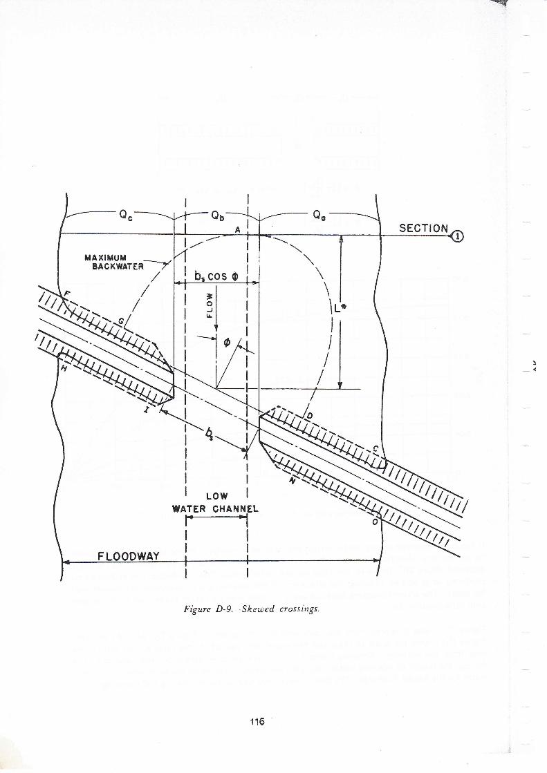
A skewed crossing is one that is other than 90o to the general direction of flow during floodstage, (Figure D-9).
(f) lUidth o.[ Constriction. b
No difficulty will be experienced in interpreting this dimension for abutments with vertical
faces since b is simply the horizontal distance between abutment faces. In the more usualcas€
involving spillthrough abutments, where the cross section of the constriction is irregular, it is
suggested that the irregular cross section be converted to a regular trapezoid of equivalent area,
asshown in Figure D-3C. Then the length of bridge opening can be interpreted as:
b=1,v
x
104
it"-.,..,".{'.-
E
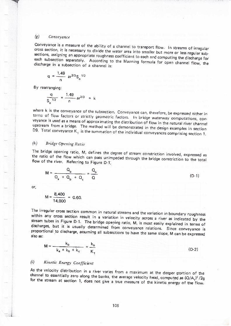
@) Conueyance
conveyance is a measure of the ability of a channel to transport flow. In strearns of irregularcross section' it is necessary to divide the water area into smailer but more or less regularsub-sctions, assigning an appropriate roughness coefficient to each and computing the discharge foreach subsection separately. According_to the Manning formula for open channel flow, thedischarge in a subsection of a channel is:
1.49g = "r2l3g
1/2
n
By rearranging:
q 1.49 ^,.{-
=-;tt''" - k
where k is the conveyance of the subsection. conveyance can, therefore, be expressed either interrns of flow factors or strictly geometric faetors. in bridge waterway computations, con-veyance is used as a means of approximating the distribution of frow in the natural river channelupstream from a bridge' The method will be demonstrated in the design ,"r.pt., in sectionDg. Total conveyance K., is the summation of the individual conveyances comprising section 1.
(h) Bridge Opening Ratio
The bridge opening ratio, M, def ines the degree of streamthe ratio of the flow which can pass unimpeded throughffow of the river. Referring to Figure D-1,
o._o-oo.D[!l =
constriction involved, expressed asthe bridge constriction to the total
(D-1)
(D-2)
Qf,
y= 8'4oo = o.60.
14,000
The irregular cross section common in natural streams and the variation in boundary roughnesswithin any cross section result in a variation in velocity across a river as indicated by thestream tubes in Figure D-1' The bridge opening ratio, M, is most easily explained in terms ofdischarges, but it is usually determined from conueyance relations. since conveyance isproportional .to discharge, aszuming all subsections to have the same slope, M can be expressedalso as:
Q"+Qo+O"
ka+kb+kcM- =ko
K1
kb
(;) Kinetic Energy Coefficient
As the velocity distribution in a river varies from a maximum at the deeper.portion of thechannel to essentiaily zero arong the banks, the average verocity head, comput{ as (e/A.,r2 /2gfor the stream at section 1, d&s not glve a true re.rure of the kiil;;;;.gi ot the ftow.
J).....-:--:t
105

Y
A weighted .Nerage value of the kinetic energyhead, above, by a kinetic energy coefficient, qr
is obtained by rnultiplyingdef ined as:
the average velocity
E (qv2 )c(, =-.' OVr
(D-3a)
Where
v. = average velocity in a subsection.q = discharge in same subsection.O = totaldischarge in river.Vl = average velocity in river at section 1 or Q/A, .
The method of computation will be further illustratedD9.
in the design examples given in Section
A second coefficient, crr, is required to correct the velocity head for nonuniform velocitydistribution under the bridge,
E (qvt )
QV,,
where v, q and Q are defined as above
V2 = av€rEge velocity in constriition =
The value of ccr can be computed and
{n-?h)
but apply here to the constricted cross section and
oiA2
c(2 can be estimated from Figure D-5.
26
Qrzz
t.8
l4
to
2.2 Q
o.5M
Figure D-s.-Aid for estimating a.,
t--,*:.i.
106

-
03.2 Definition of Symbols
Most of the symbols used in this Appendix are recorded here for reference. symbols notfound here are defined where first mentioned.
Ar = Area of flow including backwater at section l(Figs. D-28 and D-38) (sq. ft.).Anr = Area of flow below normalwater surface at section 1 {Figs. D_2ts and D-3B) {sq. ft.).Ar, = Gross area of flow in constriction below normal water surface at section 2(Figs. D-2cand D-3C) tsq. ft.).
A4 = Area of flow at section 4 at which normal water surface is reestabrished (Fig. D-2A)(sq. ft.).
, oo =
i;:T:.j:t area of piers normalto f low (between normarwater surface and streambed)
a = Area of flow in a subsection of approach channel (sq. ft.).b = width of constriction (Figs. D-2c, D-3c, and sec. D3.1 (f) ) (ft)
I b, = width of constriction of a skew crossing measured arong centreline of roadwav(Fig. D-9) {ft.).
, Cb = Backwater coefficient for flow type ll.
i cr = Freef row coeff icient for f row over roadway embankment.
' C, = Submergence factor for f low over roadway.
I e =Eccentricity=(.1 _Oc/Oa)wherel
i O" (eu,i
or (1-O"/O" ) where
O" > O".
, g = Acceleration of gravity = 32.2 (ft./sec.: ).
frr = Totaldnergy loss between sections 1 and 4 (Figs. D-2A and D_3A) (ft.).
, hu = hr-SoLr_4 = Energy losscaused by constriction (Figs. D-2A and D_3A) (ft.).'
r ht' = Total backwater or rise above normal stage at section I (Figs. D-2A and D-3A) tft.).-
, hot - Backwater computed from base curve (Fig. D-6) (ft.)
*ater surface at section 3(Figs. D-2A and D-3A) (ft.).
Ah - ht * t' h: * + So Lr--g = Difference in water surface elevation across roadway embank-ment (Figs. D-2A and D-3A) (ft.).
J = Ae/An2 = Flatio of area obstructed by piers to gross area of bridge waterway belownormal water surface at section 2 (Fig. D-7).
107I)
,."j

Ku = Backwater coefficient from base curve (Fig. D-6).
AKo = lncremental backwater coefficient for pien (Fig. D-7). L
AK" = lncremental backwater coeff icient for eccentricity (F ig. D-8).
AK, = Incremental backwater coefficient for skew (Fig. D-10).
K* - Ko + AKo + AK" + AK, = Totalbackwater coefficient for subcritical f low.
k - Conveyance in subsection of approach channel.
kb = Conveyance of portion of channel within projected length of bridge at section 1
(Figs. D-28 and D-38 and sec. D3.1 (g)).
k., k" = Conveyance of that portion of the natural flood plain obstructed by the roadwayembankments {subscripts refer to left and right side, facing downstream) {Figs. D-28and D-38 and sec. D3.1 (g) ).
K1 = Total conveyance at section 'i {sec. D3.1 (gi ).
Lr-+ = Distance from point of maximum back water to reestablishnrent of normal watersurfacedownstream, measured along centerline of stream (Figs. D-2A and D-3A) (ft.).
Lt-: = Distance from point of maximum backwater to water surface on downstream side ofroadwayembankment(Figs.D.2AandD"3A)tft.).
Lr-z = Distance from point of maximum backwater to upstream face of bridge deck (Figs.
D-2A and D-3A) (ft.)
L* = Distance from point of maximum backwater to water surface on upstream side ofroadway embankment, measurd parallel to centerline of stream (Fig. D'13) (ft.)
I = Overall width of roadway or bridge (ft.)
M = Bridge openirg ratio (sec. D3.1 (h) ).
Manning roughness coeff icient (Table D-1).
p = Wetted perimeter of a subsection of a channel (ft.)
Ob = Flow in ilortion of channel within projected lergth of bridge at section 1(Fig. D-1)(c.f.s. ).
O", O" = Flow over that portion of the natural flood plain obstructed by the roadway em-
bankments (Fig. D-'l) (c.f.s.). :
O = O. * Ou + Q" = Totaldischarge (c.f.s.).
r = a/p = Hydraulic radius of a subsection of flood plain or main channel (ft.)
So = Slope of channel bottom or normal water surface.
Vr = Q/Ar = Average velocity at section 1 (ft./sec.).
Va=o"/Aq=Averageve|ocityatsection4(ft./sec.).
Vn2 = Oy'Anz = Average velocity in constriction for flow at normal stage (ft./sec.).
Vz" = Critical velocity in constriction (ft./sec.). ,
108
I,_.-J

-!
wp = width of pier normar to direction of f row (F ig. D-7 ) (ft.).W = Surface width of stream including f lood plains (Fig. D.l) (ft.)Vr = Depth of f low at sectionl (ft.).
yq = Depth of flow at section 4 (ft.).
yn = Normal depth of f low in model {ft.).
t = An2lb=Meandepthof frowunderbridge,referencedtonormar stage,(Fig.D-3c) (ft.).Yrc = Criticaldepth at section 1 (ft.)
yac = Critical depth in constriction (ft.).
yac = Critical depth at section 4 (ft.).
c1 = Velocity head coeff icient at section I (sec. D3.1 (i) ) (Greek tetter alpha).c2 = Velocity head coeff icient for constriction (Greek letter alpha.).o = Multiplication factor for inf luence of M on incrementarbackwater coefficient for piers(Fig. D-78) (Greek tetter sigma.).
9n - hr * * h:* = for sirgle bridge (Greek letter psi.).
a., = Correction factor for eccentricity (Fig. D_13) (Greet letter omega).
0 = Angle of skew - degrees (Fig. D_9) (Greek letter phi.).
I
-.-;, -'4-
109

x
D4. COMPUTATION OF BACKWATER
D4.1 Expression for Backwatar
A practical expression for backwater has been formulated by applying the principle of conser-vation of enerly between the point of maximum backwater upstream from the bridge, section 1,
and a point downstream from the brirJEe at which normal stage has been reestablished, section 4(Fig. D-2A). The expression is reasonably valid if'the channel in the vicinity of the bridge isessentially straight, the cross sectional area of the stream is fairly uniform, the gradient of thebottom is approximately constant between sectiors 1 and 4, the flow is free to contract andexpand, there is no appreciable scoun of the bed in the constriction and the flow is in thesubcritical range.
The expression for computation of backwater upstream from a bridgs constricting the flow,is as follows:
h1 *=K*..,V-12+".,
lffi' ffi] + (D-4)
Where
hl * = total backwater (ft.).
K* = total backwater coefficient.
cl &cc2 = asdefined inexpressions (D'3A) and (D-3b) (Sec. D3-1 (i) )'
An2 = gross water area in constriction measured below normal stage (sq. ft.).
Vn2 = average velocity in constriction or Q/Anz (f.p.s').
Aa = water area at section 4where normalstage is reestablishe6 1eq. ft.).
Ar = totalwater area at section 1, including that produced by the backwater (sq. ft.).
To compute backwater. it is necessary to obtain the approximate value of h1 ' by usirg the
first part of expression (D-4)
hl* = K*o2 VnZ (D-4a)'2sThe value of A1 in the second part of expression (D-4) which depends on h1 *, can then be
determined and the second term of the expression evaluated:
" [c'-(s'] + (D-4b)
This pah of the expression represents the difference in kinetic energy between sections 4 ard 1,
expressed in terms of the velocity head, V2"z/2g. Expression (D-4) may appear ctmbersome,but this is not the case. See Example l, Section D9.
I
lj
l-:
I
110

-
D4.2 Backwater Coefficient
Two symbols are interchargeably used throughout the text and both are backwater coefficients.The symbol K6 is the backwater coefficient for a bridge in which only the bridge opening ratio,M' is considered' This is known as a base coefficieniand the curves on Figure D-6 are calledbase curves' The value of the overall backwater coefficient, K*, is likewise dependent on thevalue of M but also affected by:
1' Number, size, shape, and orientation of piers in the constriction,2' Eccentricity or asymmetric position of bridEe.with respect to the valley cross section,
3. Skew (bridge crosses stream ar other than g0" angle).
It will be dennonstrated that K" consists of a base curve coefficient, K6, to which is addedincremental coefficients to account for the effect of piers, eccentricity and skew. Thevalue ofK* is nevertheless primarily dependent on the degree of constriction of f low at a bridqe.
3.O
2.8
2.6
2.4
2.2
2.O
t.8
t.5
1.4
- 1.2Y
l.o
o.8
o.6
o.4
I
It\
1ilililtI
\IiIliirTniTil
\ OEWINGWALL ti\ \ 9(
tl)cww_llt-- tt f-
lrtir-1
il1ilililil1ilt^LENGIHS UP TO 20( FT) \1P'qw
ltlllltllllltl\-\\: soR 450 ANo 600 tvwABUTMENTS OVER2OO FI tN LEI{GTH_--
rlll\r sPILLTHROU6H
lll\
\ \\\
\ \-! \
o.2
oo
o.7o.6o.2 o.3 o.4QI o.5
M
Figurc D-6.--Bachu'ater co<:fficient base crrz,cs (subcriticar ftow).
o.8 o.9 LO
D4.3 Effect of M and Abutment Shape (Base Curves)
Figure D-6 shows the base curves for backwater coefficient, K6, plotted with respect to theopening ratio, M, for.wingwall ard spillthrough abutments. Note how the coefficient, K6,increases with channel constriction- The lower curve applies for 45o and 60; wingwall abut-ments and a' spitthrough types. curves are arso incruded for 30" *inE,"Jr .ir*"n* ard for90o vertical wall abutments for bridges up to 200 feet in length. These shapes can be identified
\*:.. -i*,3
111

from the sketches on Figure D-6. Seldom are bridgeswith the lattertype abutmentsmorethan200 feet long. For brirlges exceedirg 200 feet in lergth, regardless of abutment type, the lower
curve is recommended. This is because abutment geometry becornes less important to back-
water as a bridge is lengthened. The base curve coefficients of Figure D-6 apply to crossirgsnormal to flood flow and do not include the effect produced by piers, eccentricity and skew.
D4.4 Effect of Fiers
(o) Normal Crossings
Backwater caused by introduction of piers in a bridge constriction has been treated as an
incremental backwater coefficient designated AKo, which is added to the base curve coefficientK6 when piers are present in the waterway. The value of the incremental backwater coefficient,AKo, is dependent on the ratio that the area of the piers bears to the gross area of the bridge
opening, the type of piers (or piling in the case of pile bents), the value of the bridge opdning
ratio, M, and the angularity of the piers with the direction of f lood f low. The ratio of the waterarea occupied by piers, Ao, to the gross water area of the constriction, An2, both based on the
normaf water surface, has been assigned the letter J. In computing the gross water area, An2,
the presence of piers in the constriction is ignored. The incremental beckwater coefficient forthe more common types of piers and pile bents can be obtained from Figure D-7. By entering
chart A with the proper value of J and reading upward to the proper pier type, AK is read fromthe ordinate. Obtain the correction factor, o, from chart B for opening ratios other than unity.The incremental backwater coefficient is then:
AKo = oAK
The incremental backwater coefficients for pile bents can, for all practical purposes, be
considered independent of diameter, width, or spacing of piles but should be increased if there
are more than 5 piles in a bent. A bent with 10 piles should be given a value of AKo about 20percent higher than that shown for bents with 5 piles. lf there is a possibility of trash collectingon the piers, or piles, it is advisable to use a larger value of J to compensate for the added
obstruction" .For a normalcrossing with piers, the totalbackwater coeff icient becomes:
K* = K6 (Fig. D_6) + AKe (Fig. D"7).
(b) Shewed Crossings
In the case of skewed crossings, the effect of piers is treated as explained for. normal crossings
except for the computation of J, An2 and M. The pier area for a skewed crossing, Ao, is the
sum of the individual pier areas normal to the general direction of flow, as illustrated by the
sketch in Figure D-7. Note how the width of pier wo is measured when the pier is not parallel
to the general direction of flow. The area of the constriction, An2, for skewed crossings, is
based on the projected length of bridge, b, cos d (Fig. D-9). Again, An2 is a gross value and
includestheareaoccupiedbypien. ThevalueofJisthepierarea,Ao,dividedbytheprojectedgross area of the bridge constriction, both measured normal to the general direction of flow.
The computation of M for skewed crossings is also based on the projected length of bridge,
which will be further explained in section D4.6.
112

--Y
iIOTE :-Sroy brocing
/ln, bosad on\\ langrh b f
rhould be includtd in ridrh ot p!1.
lYtdlh of picr normOl loflor - lect
Height ot pier erpogedlo flor - tc?l
Number ol piers
a wDhnr - totor proiectcdoreo of piers normol loflor - squorc facf
Gross rol?f cross srcttonrn conslriction boscd onnormol wolcr surloce.
(Usc projaoed bridgclengfh normol lo flor
. for sker crossrngs)a9;
/An1 bosed on \\ lengf h b cos j/
wp'
hnt .
N.a, .
Anr'
Y o.2
Figure D-7.-Incremental bachwater coefficient for piers.
Ij
-..-j
-&'ai-=4lii it? iJ*,wwSKEIVED
CROSSING
Lqo/
.y yrOzr -_'ffi*a
y,'4
t.o
o.t
o.tcr
o.7
o.a
o.c
,z 7
./t z -/
# iato',?.
{.A K" .4;1o
113

D4.5 Effect of Eccentricity
Referring to the sketch in Figure D-8, it can be noted that the symbols Ou and O" at section 1
were used to represent the portion of the discharge obstructed by the approach embankments.lf the cross section is extremely asymmetrical so that O. is less than 20 percent of O" or vice
versa, the backwater coefficient will be somewhat larger than for comparable values of M
shown on the base curve. The magnitude of the incremental backwater coefficient, AK",accounting for the effect of eccentricity, is shown in Figure D-8. Eccentricity, e, is def ined as 1
minus the ratio of the lesser to the greater discharge outside the projected length of the bridge,or:
==
e=1
e= 1
_Q"Q"
ou
o.
where O. ( O,
where O" ) Q. (D-5)
Reference to the sketch in Figure D-B will aid in clarifying the terminology. For instance, ifO./Q" = 0.05, the eccentricity e = {1 - 0.05) or 0.95 and the curve fore = 0.95 in Figure D-8
would be used for obtaining AK". The largest influence on the backwater coefficient due toeccentricity will occur when a bridge is located adjacent to a bluff where a f lood plain existson only one side and the eccentricity is 1.0. The overall backwater coefficient for an extremelyeccentric crossing with wingwall or spillthrough abutments and piers will be:
K* = Ku (Fig. D 6) + AKo (Fig. D-7) + AKu (Fig. D-8).
D4.6 Effect of Skew
The method of computation for skewed crossings differs from that of normal crossings
in the following respects: The bridge opening ratio, M, is computed on the pr.ojected
length of bridge rather than on the length along the centreline. The length is obtainedby projecting the bridge opening upstream parallel to the general direction of flood flowas illustrated in Figure D-9. The general direction of flow means the direction of floodflow as it existed previous to the placement of embankments in the stream. The length ofthe constricted openirg is b, cos @, and the area An2 is based on this length. The velocity
v2^head, -F, to be substituted in expression (D-4) (sec. D4. 1 ) is based on the projected area An2.
zg
Figure D-10 shows the irrremental backwater coefficient, AKr, for the effect of skew, forwingwall and spillthrough type abutments. The incremental coeff icient varies with the opening
ratio, M, the angle of skew of the bridge O, with the general direction of flood flow, and thealignment of the abutment faces, as indicated by the sketches irr Figure D'10. Note that the
incremental backwater coefficient, AK' can be negative as well as positive. The negative values
result from the method of computation and do not necessarily indicate that the backwater willbe reduced by employing a skewed crossing. These incremental values are to be added
algebraically to K6 obtained from the base curve. The total backwater coeff icient for a skewed
crossing with abutment faces aligned with the flow and pierswould be:
K* = K6 (Fig. D-6) + AKo (Fig. D-7) + AK' (Fig. D-10A).
The procedure is illustrated in Example 2, Section D9'
114
,l

-l
O.-*q-)k-- Oo
where Q. < eo or
e =(1- wherE Qo < e.
M o'( o'8 o'9
Figure D'8'-Incremental bachu,ater coefficient .f or eccentricity.
It has been observed during model testing that skewed crossingswith angles up to 20" producedno particularly otijectionable results for any of the abutment shapes-investigated. As the angleincreased above 20o, however, the f low picture deteriorated; f tow "d""."iriai.* ,, abutmentsproduced large eddies, reducirg the efficiency of the waterway and increasing the possibilitiesfor scour' The above statement does not apply to cases where a bridge spans most of the streamwith little constriction"
Figure D-11 was prepared from the same model information as Figure D-10A. By enteringFigure D'11 with the angle of skew ard the projected varue of M, the ratio b, cos dib can beread from the ordinate' Knowing b and h1 " for a comparabre normar crossing, one can sorvefor br' the length of opening needed for a skewed bridge to produce the same amount of back-water for the desisn discharse. The chart is especiany hipfuti;;;;;;;nj'",io".nr.r.ing.
e = (1- 3:)Qo.Q.'
I
I-t
rfillrl
il1il|illtl
illilililtflltfll
115
MAXITUMBACKWATER --7
,/F/R).. / \d-'l3t*l
-I
SECTI ON
!)
S3/
Figure D-9. -Sheued crossings.
kt%
116

$fi
M
Figure D- I 0. -Incremental backwater
o.t
coefficient for skew.
.i-4
117

+lH l' oto
.dl
*,\
l._t
Figure D- I 1. -Ratioequiualent
20 30
ANGLE OF SKEW + (DEGREES)
ol' projected to normal length of bridSe, forbachu'atcr (shewed crossings).
118
D5. DIFFERENCE IN WATER LEVEL ACROSS APPROACI-I EMtsAruKMEIUTS
D5.1 Signif icance
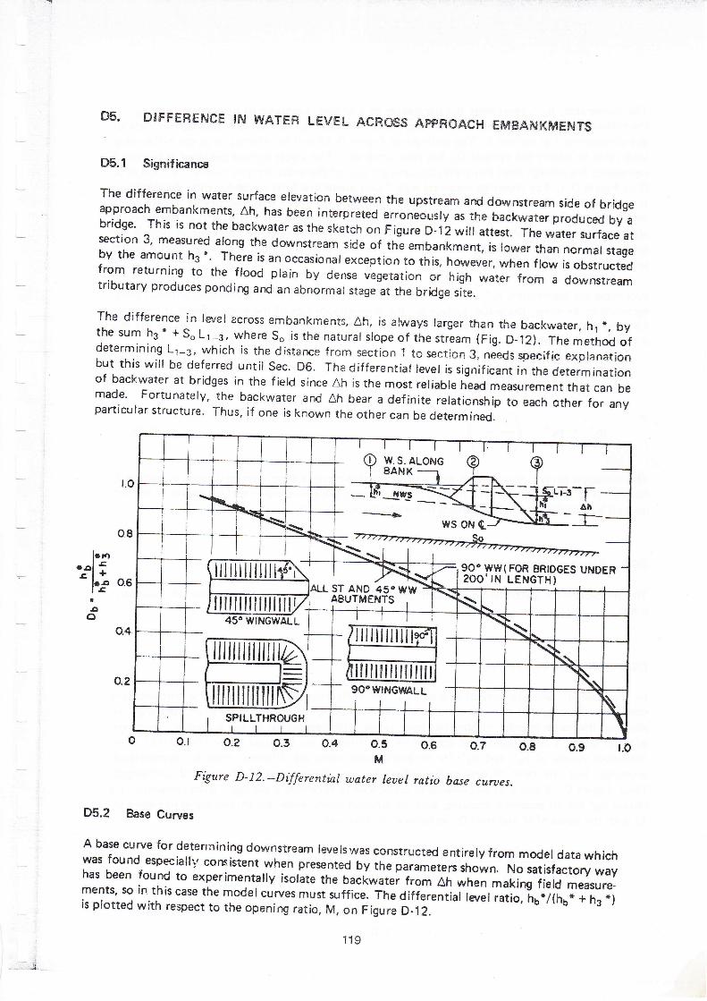
The difference in water surface elevation between the upstream ard downstream side of bridgeapproach embankments, Ah, has been interpreted erroneousry as the backwater produced by abridge' This is not the backwater as the sketch on Figure D-'r2 will attest. The water surface atsection 3' measured along the downstrearn side of the embankment, is lower than normal stageby the amount h3 *' There is an occasional exception to this, however, when flow is obstructedfrom returning to the flood plain by dense vegetation or high water from a downstreamtributary produces pondirg ard an abnormar stage at the bridge site.
The difference in larel across ernbankments, Ah, is always larger than the backwater, h1 *, bythe sum he * + So Lr--:, where So is the natural slope of the stream (Fig. D-12). The method ofdetermining L1-3, which is the distance from sectir:n I tc seetion 3, needs spee if ic explanationbut this will be deferred until sec. D6. The differential lever is significant in the determinationof backwater at bridges in the f ield since Ah is the most reliable head measurement that can bemade' Fortunately, the backwater and Ah bear a definite relaticinship to each other for anyparticular structure. Thus, if one is known the other can be determined.
o.8
btr-ol tr.-l *-l€ oe
:o
D5.2 Base Curves
A base curve for deterrnining downstream levelswas constructed entirely from model data whichwas found especiall'/ consistent when presented by the parameters shown, No satisfactory wayhas been found to experimentally isolate the backwat", f.orn Ah when makirg field measure-ments, so in this case the modelcurves must e.rffice. The differential lerrel ratio, h6*/(h6* + hs *)is plotted with respect to the openirg ratio, M, on Figure D-12.
.,,t
ST AND 45" WW
lllllulull]a
tllTlilUmrDSPILLTHROUGH
ililililt1
illtltllllltlil tJ
W. S. ALONG
90" WW( FOR BRTDGES UNDER2OO'IN LENGTH)
ilil lilil tl
lil'illil tltllgOCWINGWALL
Figure D-12.-Differential uater leuel ratio base cuntes.
't19

The numerator, h6*, represents the backwater at a bridge, exclusive of pier effect, and h3 * isthe difference in level between normal stage and the water surface on the downstream side ofthe embankment at section 3. The ordinate of Figure D-12 witl be referred to as the differentiallevel ratio to which the symbol D6 has been assigned. The water surface depicted at section 3represents the average level alorrg the downstream side of the embankment from H to I and N toO in Figure D-1. For crosings involving wide flood plains and long embankments, the distancesH to I and N to O each have been arbitrarily limited to not more than two bridge lengths. Thesolid curve on Figure D-12 is to be used for 45o and 60o wingwall abutments and all spillthroughabutments regardless of bridge lergth. The uppdr curve, denoted by the broken line, is forbridges with lengths up to 200 feet having 90o vertical wall and other abutment shapes whichseverely constrict the f low.
Assuming the backwater, h6*, has already been computed for a normal crossing, withoutpiers,eccentricity or skew, the water surface on the downstream side of the embankment is obtainedby entering the curve on Figure D-12 with the contraction ratio, M, and reading off thedifferential lwel ratio
Db=hu* + h3*
orhg* - hb* (D-6)
The elevation on the downstream side of the embankment is simply normal stage at section 3,less h3* (Fig. D-12), except for the specialcase where the entire water surface prof ile is shiftedupward by ponding from downstream or restricted f lood plains.
D5.3 Effect of Piers
The procedure for determining h3* with piers is exactly as explained in section D5.2 withoutpiers.
D5.4 Effect of Eccentricity
In the case of severely eccentric crossings, the difference in level across the embankmentconsidered here applies only to the side of the river having'the greater flood plain discharge. lnplotting th6 experimental differential level ratios with respect to M for eccentric crosirgs,without piers, it was found that the points fell directly on the base curve (Fig. D-12). Theindividual values of h6* and h3* for eccentric conditions are different than for symmetricalcrossings, but the ratio of one to the other, for any given value of M, remains unchanged.Thus, Figure D-12 can also be considered applicable to eccentric crossings if used correctly. Toobtain h3* for an eccentric crossing, with or without piers, enter theproper curve in Figure D-12 with the value of M and read D6 as before. ln this case:
hu* * Ah"*
hu*
(;)
D6=hb*+A|l3*+h3'
120

or
h3* = (hu*. + Ah"* ) (D-7)
D5.5 Drop in water surface acro.s Embankment (Normar crossing)
llaving computed h3" as described in the preceding paragraphs and knowing the total backwaterh1* (computed according to the procedure in D4), the difference in water surface elevation.across the embankment (Fig. D-12) is:
(;)
Ah - h3* * ht* + So Lr_s
where h1* is total backwater, includirg the effect of piers andnormal fall in streambed from section 1 to section 3.
(D€}
eccentricity, and So Lr_s is the
D5.6 Water Surface on Downstream Side of Embankment (Skewed Crossing).
The differential level across roadway embankments for skewed crossings is naturally differentfor opposite siles of the river, the amount depending on the conf iguration of the stream, bendsin the vicinity of the crossirg,. the degree of skew, etc. fhese factors can be so variable that ageneralized model study can shed little light on the subject.
Individual values of h1* and h3* for skewed crossings again differ from those for symmetricalcrossings, but the differential lwel ratio across the embankments at either end of the bridge canbe considered the same as for normal crossings for any given value of M. The value of M is, ofcourse, based on the projected length of bridge as explained in section D4.6. Thus, it is againpossible to use Figure D'12 for skewed crossings. The differential level ratio, D6, with orwithout piers, is obtained by entering the chart with the proper opening ratio, M. Then:
hg* = (hu*+Ahr*)(D-e)(*)
121

D6. CONFIGURAT|oru OF EACKWATER
D6.l Distancs to Foint of Maximum Backrator
In backwater cornputatbns, it will be found necesary in sorne cases to locate the point orpoints of maximum backwater with respect to the brirJge. The maximum backwater in line withthe midpoint of the br'xiee ciccurs m point A'tFig: D-lsBt, this point'beirp a dbtance, L*, fromthe waterline on the upstream skJe of the ernbankment. Where flood plainsare inundated andenrbankments congtrict the flow; the elevation oJ the water'surfrce throughout the areas ABCD*td AEFG'will beesentiafly the satrle as at point A,'where the backwater rneGurement wasmade on the models. This charasteristic has been verified from field meaurements made bythe U.S. Geological Survey on bririges where the flood plains on each side of the main channelwere no wlder than twice the bridge length and hydraulic roughness vvas relatively low.
For crossirgs with exceptiooallv wkle; rough flood plains, this€ssentiallV level ponding may notoccur.
Figure D-l3.-Distance to maxhnum bachwater.
ALv
<D
+I
: FOR ECCEI{TRIC CFG}SI}{GSwrTH a>o.7 guLTlrtY .[reU.f, fFl Ourf eVr.rb
122

Flow gradients may exist alorg the upstream side of the ernbankments due to borrow pits,ditches and cleared areas along the right-of'way. These flow gradients along embankments arelikely to be more pronounced on the falling than on the rising stage of a flood. A correlation isneeded between the water level along the upstream side of embankments and point A since it isdifficult to obtainwater surface elevations at point A in the field during floods. For the purposeof design and field verification, it has been assumed that the average water surface elevationalong the upstream side of embankments, for as much as two bridge lengths adjacent to eachabutment {F to G and D to c), is the same as at point A (Fig. D-138}.
D6.2 Normal Crossirgs
Figure D-13 has been prepared for determining distance to point of maximum backwater,measured normal to centreline of bridge.
Referring to Figure D-13, the normaldepth of f low under a bridge is def ined here as y = An2/b,where An2 is the cross sectional area under the bridge, referred to normal water surfaee, and b isthe width of waterway. A trial solution is required for determining the differential level acrossembankments, ah, but from the result of the backwater computation it is possible to make afair estimate of Ah. To obtain distance to maximum backwater for a normal channel con-striction, enter Figure D-134 with appropriate value of Ah/f and y and obtain the correspondingvalue of L*/b' Solving for L*. which is the distance from point of maximum backwater (pointA) to the water surface on the upstream side of embankment (Fig, D-138), and adding to thisthe additional distance to section 3, which is known, gives the distance L1_3. Then the com-puted difference in ls/el across embankments ts
Ah - hr**h3*+SoLr_s.
Should the computed value of Ah differ materially from the one chosen, the above procedure isrepeated until assumed and computed values agree. Generally speaking, the larger the backwaterat a given bridge the further will point A move upstream. Of course, the value of L* alsoincreases with length of brldge.
D6.3 Eccentric Crossirqs
Eccentric crossings with extreme asymmetry perform much like one half of a normalsymmetrical crossing with a marked contraction of the jet on one side and very little contractionon the other. For cases where the value of e (sec. OA.S) is greater than 0.70, enter the abscissaon Figure D-13A with Ah/V and y and read off the correspJnding value of L*/b as usuat. Nextmultiply this value of L*/b by a correction factor, o, which is obtained from Figure D.13C. Forexample, suppose Ah/V = 0.20, V = 10 and e = 0.88, the corrected value would be L*/b = 0.g4x 1.60. Distance to maximum backwater is then L* = 1.34b with eccentricity.
D6.4 Skewed Crossings
In the case of skewed crossings, the water surface elevations atong opposite banks of a streamare usually different than at point A; one may be higher and the other lowerdepending on theangle of skew, the configuration of the approach channel. and other factors. To obtain theapproximate distance to maximum backwater L'for skewed crossings (Fig. D-g), the sameprocedure is recommended as for normalcrossings except the ordinate of Figure D-.13 is read asL*/br, where b, is the full length of skewed bridge (Fig. D-9). See Exarnple 2, Section D9.
123

D7. SUPERSTR UCTURE PARTIALLY INUNDATED
D7.1 General
Cases arise in which it is desirable to compute the backwater upstream from a bridge or thedischarge under a bridge when flow is in contact with the girders. Once flow contacts theupstream girder of a bridge, orifice flow is established so the discharge then varies as the squareroot of the effective head. The result is a rather rapid increase in discharge for a moderate risein upstream stage. The greater discharge, of course, increases the likelihood of scour under thebridge. lnundation of the bridge deck is a condition the designer seldom contemplates indesign but it occurs frequently on older bridEes.
Two cases are studied; the first where only the upstream girder is in the water as indicated bythe sketch on Figure D-14 and the second, where the bridge constriction is flowing full, allgirders in the flow, as shown in Figure D-15.
D7.2 Upstream Girder in Flow (Case l)
The most logical and simple method of approach to determine the backwater effect with theupstream girder of a bridge in the f low is to assume the system acts like a sluice gate.
Using a common expression for sluice gate f low
o = coulrz fzo
O = total discharge-c.f.s.
Cd = Coefficient of discharge
bry = net width of waterway (excluding piers)
Z = vertical distance - bottom of upstream
- ft., and
Yu = vertical distance-upstream water surface
(D-10)
_ ft.girder to mean river bed under bridge
to mean river becl at bridge-ft.
lz\Y,- T*
*tVr22s )]
'"
where
For case l, the coefficient of discharge C6, is plotted with respect to the parameter Yu/Z onFigure D-14. The upper curve applies to the coefficient of discharge where only the upstreamgirder is in contact with the flow. By substituting values in expression (D-10), it is possible tosolve for either the water surface upstream or the discharge under the bridge, depending on thequantities known. lt appears that the coefficient curve {Fig. D-14) approaches zero asYu/Zbecomes unity. This is not the case since the limiting value of Yu lZ for which expression(D-10) applies is not much less than'1.1. There is a transition zone somewhere betweenYulZ= 1.0 and 1.1 where free zurface flow charqes to orifice flow or vice versa. The type offfow within this range is unpredictable. For Yu lZ = 1.0, the flow is dependent on the naturalslope of the stream, while this factor is of li-ttle concern after orifice flow is established orY,rlZ > 1.1.
124

!VS. ALONG EMBANKMENTS
t.2 t.3,.., t.4 1.5 1.5 1.7 l.gYu
Y3
Figure D'14 - Discharge coelfrcients for upstreqm girder in flotu (case I)
-rz
rI
thtrrrrS
Y3
0.6
o.5
o.4
o.3
o.2
o.l
o
=5++j:?f,
125

/
B/
/
,/
,/
"/
!v
t7
toLo
lOr
04 0.6Ah__
v
l.oo.8
o8
t(,
o.azYu
Figure D-15 - Discharge coelficient for all girders in flow (case II)
aa
a
feo
la o
;W ASUTIENTSs r ASuTu€tirTS
I
or v'aT
e
t{.w.s"l
tLofiG €r8AjrtxilElla-
4h ir"t-.J-
I
YUI
T
,I
Ltt pbr rcnnL rs.
* Dr,L,)r-,7m7rV7727V2>-r,vv77v. 7
Ao ca\zJeo6-h
126
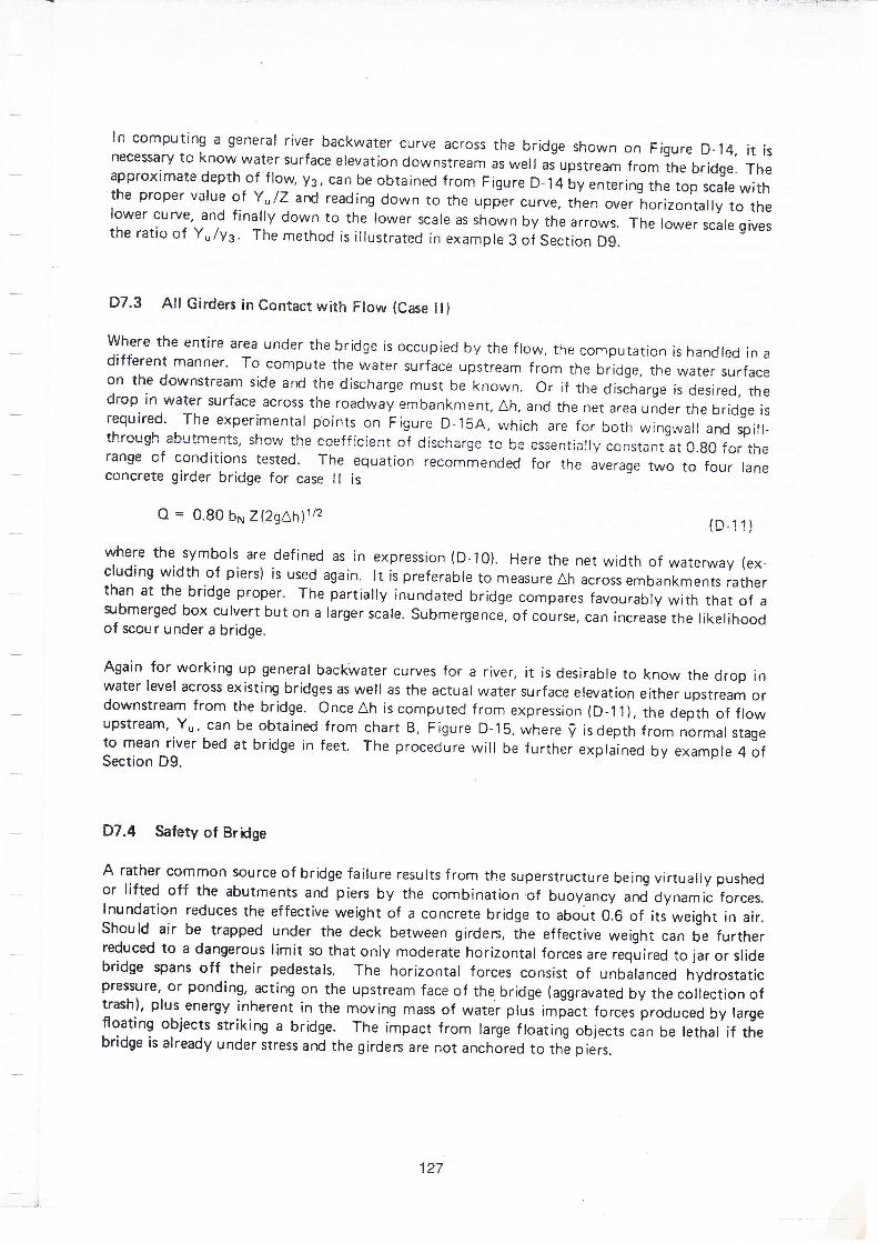
ln computing a general river backwater curve across the bridge shown on Figure D-14, it isnecessary to know water surface elevation downstream as well as upstrean from ihe bridge. Theapproximate depth of flow, !3, cafi be obtained from Figure D-14 by enterlng tne top scale withthe proper value of Yu/7 arfr reading down to the upper curve, then over horizontally to thelower curve, and finally down to the lower scale as shown by the arrows. The lower scale givesthe ratio of Y,/y3. The method is iilustrated in exampre 3 of section Dg.
D7.3 All Girders in Contacr with Flow (Case ll)
where the entire area under the bridge is occupied by the flow, the computation is handled in adifferent manner' To compute the water surface upstream from the bridge. the water surfaceon the downstream side and the discharge must be known. or if the disJharge is desired, thedrop in water surface across the roadway embankrnent, Ah, and the net area underthe bridge isrequired' The experimental points on Figure D 15A, which are for both wingwall and spill-through abutments, show the coeff icient of discharge to be essentially constant at 0.g0 foi- therange of conditions tested. The equation recommended for the average two to four laneconcrete girder bridge for case ll is
Q = 0.80 bx Z{2gAh)1/2f n-111
where the symbols are defined as in expression (D-10). Here the net width of waterway (ex-cluding width of piers) is used again. lt is preferable to measure Ah across embankments ratherthan at the bridge proper. The partialiy inundated bridge compares favourably with that of azubmerged box culvert but on a larger scale. Subm.rg"n"., of course. can increase the likelihoodof scour under a bridge.
Again for working up general backwater curves for a river, it is desirable to know the drop inwater level across existing bridges as well as the actual water surface elevation either upstream ordownstream from the bridge. OnceAh iscomputed from expression {D_1,1), the depth of flowupstream, Yr, can be obtained from chart B, Figure D-15, where ! isdepth from normal stageto mean river bed at bridge in feet. The procedure will be further explained by example 4 ofSection D9.
D7.4 Safety of Bridge
A rather common source of bridge failure results from the superstructure being virtually pushedor lifted off the abutments and piers by the combination.of buoyan"y unJ dynamic forces.Inundation reduces the effective weight of a concrete bridge to about o.g of its weight in air.Should air be trapped under the deck between girdem, the effective weight can be furtherreduced to a dangerous limit so that oniy moderate horizontal forces are required to jar or slidebridge spans off their pedestals. The horizontal forces consist of unbalanced hydrostaticpressure, or ponding, acting on the upstream face of the bridge (aggravated by the collection oftrash), plus energy inherent in the moving mass of water plus impact forces produced by largefroating objects striking a bridge. The impact from large floating objects can be lethal if thebridge is already under stress and the girden are not anchored to the Diers.
127

D7.5 Flow Over Roadway
In cases where bridge clearance is such that girders become inundated during floods, there is agood possibility that flow also occurs over portions of the approach roadway. Should it bedesired to determine the discharge flowing over the roadway, Figure D-16 can be used.
To determine the discharge flowing over a roadway. first enter curve B (Figure D-16)with Hiland obtain the free flow coefficient of discharge C1. Should the value of Hll be less than 0.15.it is suggested that C1 be read from curve A of the same Figtire. lf submergence is present(e.9., if D/H is larger than 0.7) enter curve C with the proper value of submergence in percenrand read off the submergence factor Cr/C1. The resulting discharge is obtained by substitutingvalues in the expression:
o = cr1P3/2 cr/ct, (D-1 2)
where L represents the length of inundated roadway, H is the total head upstream measured
above the crown of the roadway and Cr and C, are coefficients of discharge tor free flow and
with submergence, respectively. Where the depth of flow varies along the roadway, it is
advisable to divide the inundated portion into reaches and compute the discharge over each
reach separately. The process, of course, can be reversed to aid in determining backwater fora combination of bridge and roadway.
128

P€RCENT SI,E'YERGENCE
cv€.RALL O. Cr t..r(l/z.cs./c,
o/H X too
90
t^[3.o.rF
sczi-3.@l-
2rdFt*r2.9f 1
,nlle soLl
a.l
IJo..t
z<j
l.rlo{
g9q THS C:tJRlrE FOf, FR€E FLOilco€FFlcfENTs vilni H/t RATtos<o,5.
A
_.._.L_ i- | i i | | .l . I I | | | | | Iot t2 t.6 2p 2.4 z.e. 32 5.6 40I€AO o?{ ROAryIV H il FEET
Figure D'16 - Discharge cofficients for florv over roadtvay embanlonents
129

D8. BRIDGE DESIGN FROCEDURE
D8.1 Site Study Outline
The following outline is presented to aid in organizinE and collecting the necessary field datafor a bridge site investigation:
1. Location map to show proposed highway alignment and reach of riverto be studied.
2. Vicinity map showing flood f low patterns, cross sections of stream, location of proposedbiidge and relief openings, and alignment of piers.
(i) Map showing 1- or 2-foot contours, stream meanders, vegetation and manmadeimprovements.
(iii In some cases, cross sections perpendicular to flood flow are acceptabie in lieu ofthe map in (i); at least three cross sections are desirable: one on the centreline ofthe proposed bridge, one upstream and one downstream from the proposed bridgeat from 100 to 500 foot intervals.
3. A full description of existing bridges both upstream and downstream from proposed
crossing (including relief and overflow structures).
(i) Type of bridge, including span lengths and pier orientation.
(ii) Cross section beneath structure, noting stream clearance to superstructure and
skew or direction of current during f loods.
(iii) All available flood history-high water marks with dates of occurrence, nature offlooding, damages and source of information.
(iv) Photographs of existing bridges, past floods. main channels and flood plains and
information as to nature, streambed and stability of banks.
4. Factors affecting water stage at bridge site.
(i) High water from other streams"
(ii) Reservoirs-existing or proposed and approximate date of construction.
(iii) Flood control projects.
{iv) Tide.
(v) Other controls.
130

D8.2 Stago Discharge
It is important that the normal stage of a river for the design flood be determined as accuratelyas possible at the bridge site. This may be accomplished inieveral ways, but where possible it isbest to establish it from a stag*dischaige rating curve based on stream-gauging records colectedin the vicinity of the brklge site. whlre stagedischarge records are lacking for the stream inquestion' the usual procedure is to locate high water m-arks of floods by consulting people wholive in the vicinity of the proposed bridge site. Flood information supplied by local residents isoften inaccurate, but may be consirjered reliable if confirmed by other residents.
It is then necessary to find a means of relating stage to discharge. This can be done by theslope-area method, a simplifiedvariation of which w*ill be found illustrated in Example I sectionD 9' Extreme care must be exercised both in the collection of f ield data and in the manner inwhich it is processed if glaring discrepa.cies are to be avoided in the f inal result. rn many caseswhere records are lacking, it is advisabie to arrange for the installation and maintenance of atemporary stream gauge at or near the bridge site several years in advance of construction. Evena single reliable point at an intermediate stage can be of inesiimablevalue in the preparation ofa stage-discharge curve.
D8.3 Channel Roughness
A rnatter of prime importance in bridge backwater or slope-area computations is the ability tocvaluate properly the roughness of the main channel and of the flood plains; both are subiect toextreme variations in vegetal growth and depth of flow. As a guide. values,rf the Manningroughness coefficient, n, as commonly encountered in practrce, are tabulated for variousconditions of channel and flood plain in fable D-1. Since tfre practicing engineer in this countryis familiar with the Manning roughness coeff icient. the Manning equation has been chosen foruse here' ln interpreting roughness coeff icients from Table D-i, it shoutd be kept in mind thatthe value of n for a small depth of f low, especially on a f lood plain covered wiirr grass, weeds,and brush, can be considerably larger than that for greater f row depths over the same terrain.On the other hand,'as the stage rises in a stream with an aliuvial bed, sand wavesdevelop whichcan increase the value of n. lt is, therefore, suggested that the notes acccmpanying Table D-1be carefully considered 'along with the tabulation.
131

Table D-1"-Manning's Roughness Coefficient for Natural Stream Channelsl
A. Minor Stream (surface width at f iood stage
1 . F airly regu lar sect io n;
a. Some grass and weeds, little orb. Dense growth of weeds. depth
B. Flood plains (adjacent to natural streams):
1. Pasture. no brush:
a. Short grass
b. H igh grass
cu ltivated areas:
( 100 ft.):2
no brushof f low materially
ltlanning'sn range
0.030-0.035
0.035-0.05
0.01-0.02
0.04-0.050.05-0.07
0.030-0,0350.035-0.050.035-0.045
0.05-0.070.06-0.08
0.10-0.16
0.04-o.050.06-0.08
0.10-0.12
s'"ui;'than weed height
lrregular section, with pools, slight channel meander; channels (a)
and (b) above, increase all values about
3. Mountain streams, no vegetation in channel. banks usually steep,trees and brush along banks submerged at high stage:
a. Bottom of gravel, cobbles. and few bouldersb. Bottom of cobbles with larqe bounders
2.
?
4.
5.
6.
Heavy weeds, scattered brush
Light brush and trees:3
Medium to dense vegetation:3
Cleared land with tree stumps, 100-150 per acre:
a. No sprouts
trees, little undergrowth:
Major stream (surface width at f lood stage ) '100 feet): Roughnesscoefficient is usually less than for mirror streams of similar descriptionon account of less effective resistance otfered by irregular banks orvegetation on banks. Values of n may be somewhat reduced. Followgeneral recommendationsl if possible. The value of n for larger streamsof mostly regular section, with no boulders or brush, may be in thera nge 0.028-0.33
lWith channel of alignment other than straight, loss of head by resistance forces will be increased. A stnali increase in value ofn may be made lo allow for the additional loss ol energy.
2The tentatiue values of n cited are princrpalty cterived !rom meosurernentsmde on fairly short but straight reaches of naturalstreams. Where slopes caiculated from tlood elevations along a consherable length of channel, involving meanders and bends,
are to be used in velociry calculations by th,; Manning formula, the value of n must be increased to provrde f or the additionalloss of energy caused by bends. All values in the table musi be so increased. The increasemav be in the range of perhaps 3 to1 5 percenr.
?"The presence ol foliage on trees and brush under f lood stage will materially increase the value of n. Therefore, roughness
coefficients for vegetation in leaf will be larger than for bare branches. For trees in channel or on banks, and lor brush onbanks where submergence of branches increases v/nh depth of flow, n will increase with risirg stage.
b. With heavy growth of sprouts
7. Heavy stand of timber, a few down
c.
132

1.
2.
3.
D8.4 Bridge Backwater procedure
The following is a brief step-by-step outlin€bridge constriction:
for determining the backwater produced by a
3.tJ;t#:t the magnitude and frequencv of the discharge for which the bridge is to be
Determine the stage of the stream at the bridge site for the design discharge.Plot a representative cross section of stream for design discharge at section l, if notalready done under step 2' tt streim channer is esse-ntiaily stra6ht and cross sectionsubstantially uniform in the vicinity J the bridge, tr,, ""ir*r cross section of the streamat the bridge site may be used for this purpose.
subdivide the cross section plotted in step 3 according to marked charges in depth offlow and changes in roughness. Assign values of Marining roughness coefficient, n, to:;:iiff::.tion
(Tabre D-1i. €xperience and carefurjudsment are necessary in serectirq
.t""J:rti::,:onvevance and then discharge in each subsection (method is demonstrated in
Using cumulative conveyance and discrrloe at section 1, computeslope of stream, so.should the computed slope vary rnore than 2s percent irom the actuar srope, reassignvalues of the roughness factor, n, and repeat conveyance c€mputations.
?,"l"Jl,tr #:i: of kinetic enersv coefficient, cr (method is iilustrated in Exampre
Plot natural cross section under proposed bridge based on normal water surface fordesign discharge, and compute gross water area (including area occupied by piers).compute bridge openirg ratio, M (section D3.1(h), observing modified procedureforskewed crossings, (Section D4.6).
obtain value of K6 frorn base curve in Figure.D-6 for symmetrical normal crosings.lf piers are involved' computevalue'of J (sec. D4.4) and obtain incre'nentalcoefficient,AKo' from Figure D-7 (noie ,'",r,oa outrined for skewJ cissings, sec. D.4.4 (b) ).lf eccentrjcity is
,Tu.r.:. compr.rte value of e (Sec. D4.5) and obtain incrementalcoefficient, AK", from Figure D-g.
lf a skewed crosing is involved, observe proper procedure in previous steps, then obtainincrementar coefficient, AKr, for proper abutment type from Figure D-10.Determine total backwater coefficient, K*, by adding incremental coefficients to basecurve coefficient, K6.
Estimate cz from Figur.e D_5, then make allowance for
:fffiffi ""
i",?f:T:[,TX*nl_i,:f h m a y I eao to r; JY "$;]:l,l"TT:il]i?Compute backwater by expression (D_4), section D4..|.Determine distance upstream to maximum backwater from Figure D-.,3 and converrbackwater to water sjrface elevation at section 1 if computations are based on normalstage at bridge.
4.
5.
6.
7.
8.
9.
10.
11.
12.
13.
14.
15.
16.
17.
133

D9. ILLUSTRATIVE EXAMPLES
D9.1 General
A better understanding of the procedures for computing bridge backwater can be gained fromthe illustrative examples in this section. The examples dealwith the following phases of design:
1. Example 1 comprises a simple normal crosing; the steps closely follow the outline ofdesign procedure listed in section D8.4.
2. Example 2 should help clarify the procedure recommended for skewed crossings.
3. Example 3 demonstrates how discharge or differential water level across bridge embank-ments can be determined when the upstream girder is in the f low.
4. Example 4 is same as example 3 with the structure partially inundated.
D9.2 Example 1: NormalCrossing
(o) Giuen
The channel crosing shown in Figure D-17 with the following information: Cross section ofriver at bridge site showing areas, wetted perimeters, and values of Manning, n; normal watersurface for design = El. 28.0 ft. at bridge; average slope of river in vicinity of bridge So = 2.6 ft./mi. or 0.00049 tt./tt.; cross section under bridge showing area below norrnalwater surface and
width of roadway = 40 ft.
The stream is essentially straight, the cross section relatively constant in the vicinrty of thebridge, and the crossing is normal to the general direction of flow.
(b) ToFind
la. Conveyance at section 1.
lb. Discharge of stream at El. 28.0 ft.
1c. Velocity head correction coefficbnt, crt.
1d. Bridge opening ratio, M.
1e. Backwater produced by the bridge.
lf. Water surface elevation on upstream side of roadway embankment.
lg. Water surface elevation on downstream side of roadway embankment.
FtJU|lIzF
__slrlUJ
134
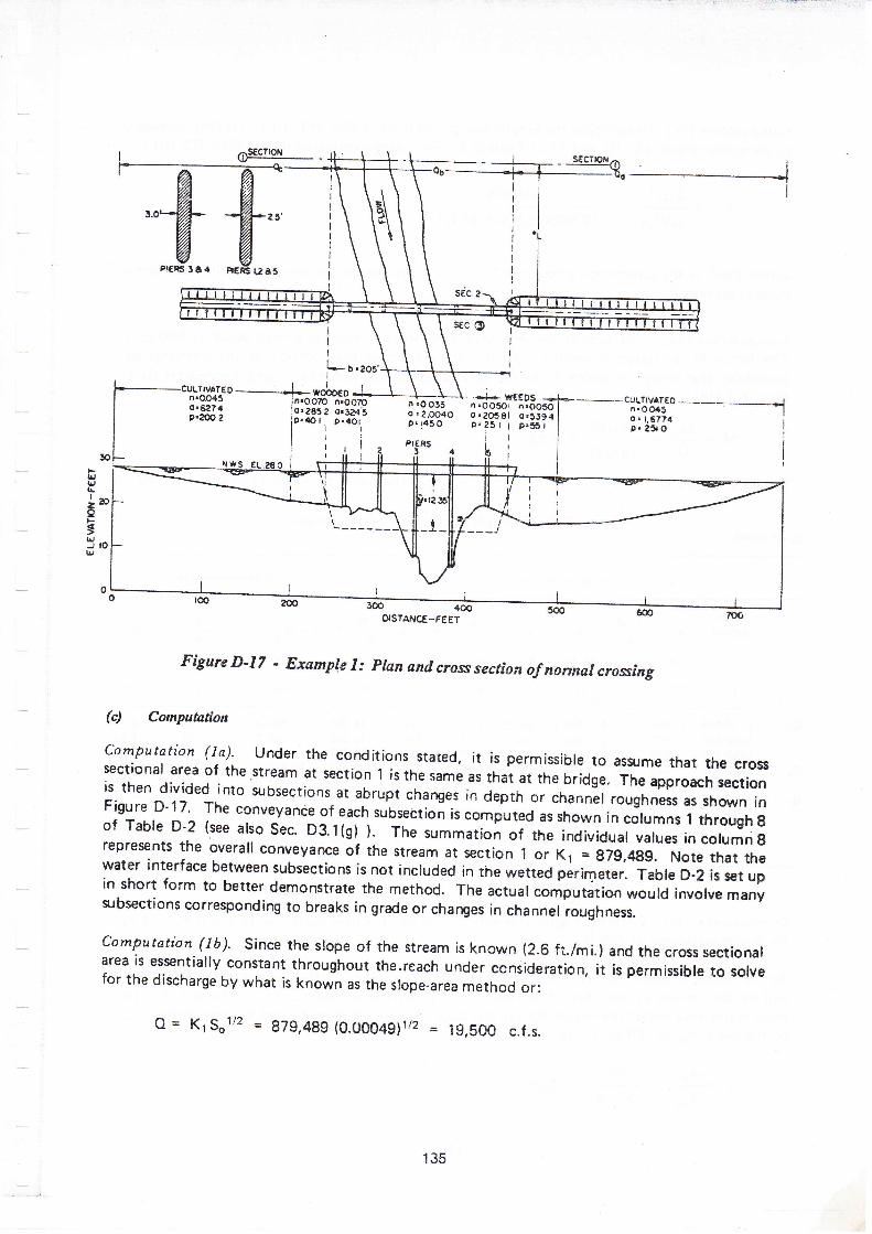
^sEcTOilU.-
'"'%PrEns I a 4
CULTIVATEOn.OO45o'6?74p.oe
sEC ?
sEc o
n .o o35o '?,OO4Oe' lll o
PI€RS34
3@ 4OOOSTANCE-F€Er
o . 1.6774p. 23r O
Figure D-r7 - Exampre I: pran and cros section of normar crosing
(c) Conputation
computation (1a)' Under the conditions stated, it is permissible to assume that the crosssectional area of the .stream at section 1 is the same as thai at the bridge. The approach sectionis then divided into subsections at abrupt changes in depth or channel roughness as shown inFigure D-17' The conveyance of each subsectioi i, compuied as shown in cJlumns t through gof rable D-2 (see also sec' o3.1(g) ). The summation of the individual values in columngrepresents the overall conveyance of the stream at section I or K1 = g79,4gg. Note that thewater interface between subsections is not included in the wetted perimeter. Table D-2 is set upin short form to better demonstrate the method. The actual computation would involve manysubsections corresponding to breaks in grade or changes in channel roughness.
Computation (1b). Since the slope of the stream is known (2.6 ft./mi.) and thecrosssectionalarea is essentially constant throughout the.reach under consideration, it is permissible to solvefor the discharge by what is known as the srope-area method or:
Q = Kr Sotrz - B7g,4gg (0.00049)r/2 = 19,s00 c.f.s.
l- o . eos'I
-+ts\looo€D
-].in.ooTo nrooTolo.?85? o.3Aas
io'*,i o..o'i
135

Computation (1c)..To compute the kinetic energy coefficient (Sec. D3.1(i) ), it is first necessary
to complete columns 9, 10, and 11 of Table D-2; then, using expression (D-3a) (Sec. D3.l(i) ):
Equ2 374,895qr=-=-' ov2nl 19,500(19,500/5,664)2
= 1.62
where Iqv2 is the summation of column 11, and.Vnl repr€s€nts the average velocity for normalstage at section 1.
Computation (1d). The sum of the individual discharges in column g must equal 19,500 c.f.s.' The factor M, as stated in section D3.1{h), is the ratio of that portion of the discharge ap-proaching the bridge in width b, to the total discharge of the river; using expression (D-l)(Sec. D3.1(h) ).
, Q^ 12.040M=*=-::--:-=o'62u 19,500
Entering Figure D-5 with crr = 1.62 and M = A.62, the value of tz is estimated as 1.40.
Table D-2.-Example 1: Sample computations.Sr=0.00(X9
C,omputation (ta) Compuntion (lc)
Sub---: l.{9 q I '19 - k os€ctron a p r=- r,lt k=--ar|tt S=Q; u-! Cdtn p n ,\1 Q
sq. ft. ft. ft cfs fps
(r) (2) (3) (4) (5) (6) (.7) (8) (e) (10) (ll)
Q.- -.- I 0-200 0 045 33.0 627.4 2c/i .2 3 134 2 t42 44.349 9E[t.3 1.57 2,124l20o-2{0 .070 2r.2 2852 {0.t 7.tr2 3698 22.359 4957 r.71 l,50l(z+uzao .020 2r.z 324s 40 1 B.os2 4.031 27,7J2 614.8 r.$ 2,196
o--- "-{280-{20 .035 12 5 z.W.O t{5 0 13 821 5.7s9 490,492 10,875.2 5.{3 320.65{llzo-<ls .0s0 n.7 2os8 2s.t 8199 4.066 24.8s2 ssl.o 2.68 a,gsE
A.---" /lls-soo .0s0 n] 939 4 ss t 9.289 {.s26 73,to9 1.62s.{ 3.01 11,726lsoo-zso .o4s 3J.0 1,627.4 2it.0 6 683 B.ilB 196,396 {,3s4.6 2.60 29,136
zl"=5,6fi1 .7 sq. ft. Kr :,i79,{89 Q = 19,5OO.0 c.f.s. &d=374,E95
,{^: =2,53{ sq. ft. Qr :12. O{0 c.f.s.
Computation (1e). Entering Figure D-6 with tul = 0.62, the base curvecoefficient is K6 = 0.72for bridge waterway of 205 ft.
As the bridge is supported by f ive solid piers, the incrernental coeff icient (AKe) for this effectwill be determined as described in section D4.4. Referring to Figu.re D-17 and Table D-2, thegross water area under the bridge for normal stage, An2, is 2,534 sq. fr. and the area obstructedby the piers, Ao, is 180 sq. ft.; so:
A^ 180J= '=-=0.07 1
Anz 2,534
136

Entering Figure D'7A wlth J = 0.071 for solid piers, the reading from ordinate is AK = 0.13.This value is for M = 1'0' Now enter Figure D-zg ana obtain the correction factoro, forM =0'62 which is 0.84. The incremental backwater coefficient for the five piers, AKo = AKo =0.13x0.84=0.11.
The overall backwater coeff ic ient :
K' = Ku * AKo = 0,12 + 0.11 = 0.g3,
o 19.500vn2 = -- =
--- = 7.70 f.p.s.Ane 2,534
andrtZY n2
= o.9z ft.2s
Using expression (D-4a) (sec. D4.1), the approximate backwater wiil be.
;1. oz-V2nz
= 0.g3 x 1.40 x 0.92 = 1.07 ft.29
v.vv A r.rv A v.-rz - LU/ It. (D-4a)
Substituting values in the second half of expression (D-4) for difference in kinetic energybetween sections 4 and 1 (Sec. D4.1) where Anl = 5664 sq. ft. = Ae ,
Ar = 6384 sq. ft., and An2 = 2534 sq. ft.,
(D-4b)
[ /z,ssq\ . fz5sa\ z]t'oz L\r,../ - \;5o| J
0.s2 = 1.62 x 0.042 x 0.e2 = 0.06 ft.
Then total backwater produced by the bridge is
ht * = 1.07 + 0.06 = 1.13 ft. (D_4)
Computation ([fl- The statement was made (in Sec. D6.1) that the water srface on theupstream side of the roadway embankment will be essentially the same as that at section l.Thus, to determine the backwater elevation it is first necessary to locate the position of section1, which is accomplished with the airi of Figure D-13.
From preceding computations :
b = 205 ft.
andA'u 2.5Uy= "-b 205
c [s' Hl+-or
137

It is necessary to assume the total drop across the embankments for a first trial (Ah is assumed
as 1.9 ft.l. Entering Figure D-13 with
and
and
ah 1.90
- = = 0.154
t 12.36
! = 12.36,
L*_ = 0.79b
L* = 0.78 x 205 = 160 ft.
The drop in channel gradient between sections 1 and centreline of roadway is then SsLl_( =0.00049 (160 + 30i = 0.093 ft. Thewatersurface elevation at section 1 and along the upstreamside of the roadway embankrnent will be:
El. 28.0 + So Lr- {+ hi = 28.0 + 0.09 + 1.13 = Et. 29.2 ft.
Computation (ld. The first step in determining the water surface elevation at section 3 istocompute the backwater for the bridge in question without piers, as explaineb in Section DS.
hb' = ;qo o2V2n2
= 0.72x 1.40 x 0.92 = 0.g3 ft.2s
Entering Figure D-12 with M = 0.62, the differentiai levelratio for the bridge (without piers) is:
hrDb = "b =0.58,ho' + h3'
so
h3. = n,.(a ) =0.e3fu ) =0.67rt. (D-6)
The placing of piers in a waterway results in no change in the value of h*3 provided otherconditions remain ihe same {Sec. D5.3), so h*3 (with piers) also equals O"OZ tt. The watergrface elwation on the downstream side of the roadway embankment will be essentially
El. 28.0 - 0.67 = 27.33 ft.
The drop in water surface across the embankment is then
Ah = 29.22 - 27.33 = l.Bg ft.
Since Ah was assumed as 1.90 ft., the computed water surface elevationsabove ir" s.tistactory.Should the computed value of Ah be materially different from that assumed, another trialwillbe necessary.
138

D9.3 Example 2: Skewed Crossirg
(o) Ciuen
A skewed bridge, Figure D-18 on the site chosen in examole
From example 1:
Q = 19,500 c.f.s. for N.W.S. = 2g.0,b = 205, So = 0.00049, q1 = j.62, M = 0.62,Aa =. 5,664 sq. ft., 41 = 6,3g4 sq. ft. and / = 40 ft.
^ sEcTroN I*/- -
-|
-
Q= l9,5OOcfsN.fy.s. 28.oAp-22O SO.FT
5I.]
Figure D-18.-Example 2: Plan for shewed crossittg
139
1. rather than a normal crossino.
| _ SECTON^
r ---1UI
-J---oo
bs cos * =192'

(b) To Find
F ind
2a. Length of skewed bridge required to produce essentially 1.1 feet of backwater as
occurred in example 1.
2b. The backwater for bridge length chosen.
2c. The approximate water level at point A on section 1.
(c) Computation
Contputution (2a). The design discharge and normal stage at bridge site are known. The sameprocedure demonstrated in example 1 is followed, with exceptions as noted. First, the generaldirection of flow in the river at the bridge site for the design flood, without constriction, is
determined. Next, the position and extent of roadway embankments and the type of abutmentare superimposed on the stream as illustrated in Figure D-9. The angle of skew is measured,which is 40" in this case; then the bridge opening is projected upstream, normal to the directionof flow, to section 1.
Entering Figure D-1'1, with d = 40o and M = 0.62.
b.Cosd= 0.935.
b
b'Cos@ = 0.935 x 205 = 192 ft.,
192b, =
-=
250 ft. (aPProx.).0.766
Computation (2b). The actual backwater produced by the skewed bridge, 250 feet long, will becomputed as a check on the above determination as well as to demonstrate the method ofprocedure. Conveyance and area are both plotted with respect to distance across flood plain atsection 'l on Figure D-19. The information needed to construct the chart came directly fromTable D-2 which was prepared in connection with the solution of example 1.
The first step is to locate the position of the skewed bridge on Figure D-19 and lay off theprojected length, b, Cos@, as shown. Then M is computed as follows:
na= ! =K1
600,000 - 70.000
879.489= 0.60
From Figure D-6, the backwater coeff icient, Kb = 0.77.
Note that an extra pier has been added and all are parallelobstructed by piers, Ao, is now 220 sq. ft. The projectednormal water surface, from Figure D-19 is
to the direction of f low. The areaarea under the bridoe referenced to
140

Ana = 3,400 - 1,000 = Z,4OO sq. ft.
and
J= Ao - 220 =0.092An2s 2,4W
consulting Figure D-7, the incrementar backwater coeff icient for piers
AKo=0.18x0.8=0.1S
Entering Figure D-10A with M = 0.60 and O = 40",
AK, = -0.19.
The total backwater coefficient for the skewed bridge is then
K* = Ko * AKo + AK, = 0.77 + o.ls - 0.19 = 0.73,
o 19,500v62 = '- = -- = 8. 13 f.p.s.,Anz 2,4W
Y2n2/2g = 1.03
and from Figure D-S,
cr2 = 1.40
Using expression (D'4a) (sec. D4.1) the approximate backwater wiil be
t- \12K*
*1" * = 0.73 x 1.40 x 1.03 = 1.0b ft.29 "vu r'' {D4'a)
Substituting values in the second half of expression (D-4),
ll \cl l(t\' - A.\'l-u''' L\aol \^J J ,,
=162 lffi) '-(#) '] 103
= 1.62 x 0.037 x r.o3 = 0.062 (D-4b)
The total backwater for the skewed brirJge is
hr* = 1.0S + 0.06 = 1.11 ft. (D_4)
141

Computation (2c). For skewed crossings the distance to maximum backwater, L*, has beenchosen arbitrarily as equal to br, so:
SoLr-C_ = 0.00049 (250 + 30) = 0.14 ft.
The water level at point A is thus
El. 28.0 * hr' + SoLr_ g = 28.0 + 1.1'l + 0.14
= El. 29.2 ft.
In the case'of a skewed crossing, the water level along the upstream face of the two embank-ments will be different and neither need correspond to that at point A.
345DISTANCE IN HUNDREOS OF FEET
Figure D-19 - Examples 7 and 2: Conveyance and area at section 7
F!I4T
()lrJo
3ktrj(r
I
?o
(tIxIu8oF
lr,96a.
lrj
z8cI
-v.
bs cos +
Q- 19,50J cf s --N.YflS = EL.28.O
r42

D9.4 Exampfe 3: Upstream Bridge Girder in the Flow
(") General
when computing general backwater curves for a river, it is necessary to know within reasonablelimits the amount of pondirg which occurs at bridges which constrict the'flow during floods.The bridge backwater, the downstrearn water surface, and the drop in level across bridge em-bankments, where clearance of superstructure is not a problem, have been treated in thepreceeding examples' Examples 3 and 4 pertain to'bridges in which the flow is in contact withthe superstructure.
(b) Given
Plan and cross section of the bridge of example t (Fig. D-17) and the centreline prof ile shownon Figure D-20. For this example, suppose that the superstructure is lowered so the bottomof the upstream girder is at erevation 2g.0 or at the normarwater surface.
a,Vra
29
W.S. ALONG EMEANKMENT
i--":*+ AhEL.2?98
ACTUAL W"S.
(r)
3a.
3b.
3c.
Q'|9,5OO CFS. Yu
Figurc D-20 .Exampk,.7: Ltltstrt,an Girrlt,r t.n Flow
Find
The approximate water surface arong the upstream face of the embankment.The approximate water surface along the downstream face of the embankment.The drop in water lever across the bridge embankment without scour.
Computation (3a). The pertinent quantitles from example 1 are:
O = 19,500c.f.s., So = 0.00049, i = 12.35 ft.b - 205 ft., Wo = 14 ft., Anr = 5,664 ft.2Vnt = 19,500/5,664 = 3.45 f.p.s., cr = '1.62 anda1V26/2g = 0.30 ft.
The discharge expression from Section D7.2 is:
143

( (D-10)
29bru Co2'
As a first trial, assumeYr/Z = 1.12; enter the upper curve on Figure D-14 with this value, andread C6 = 0.380.
Substituting in equation (D-10)
Yu = =, ',=,(tni?o-0 .].,, '. '..,. + 12'35 -0.30-
64.4 (191 x 1235l|2 (0.380)2 2
- 1'061- + 6.18 - o"3o(0.38)'
In Figure D-14 hu* =Y, - V
h,,' = 13.25 - 12.35 = 0.9 ft.
Then 41 = 5,664 + 77O {0.9) = 6,357 ft.2
V1 = 19,500/6,357 = 3.07 f.p.s.
v t2 l2g = 0.146 and
C'rv12/2g= 1.62 x 0,146 = 0.,236.
The corrected value of
Y, = 7.37 + 6.18 - 0.236 = 13.31 ft. and
Y"lZ = 13.31112.35 ='1.078
which does not agreti with the assumed value (1.12l,.
Next assume Y "/Z = 1 .10, then C6 = 0.370 (F ig. D- 14),
Yu = 1.061/(03712 + 6.18 - 0.24
= 7.75 + 6.18 - O.24 = 13.69 ft.
hu* = 13.69 - 12.35 = 1.34 ft. and
Ar = 5,664 + 1.34 x 770 = 6,696 ft.2
[,L
qz
,2,
bruZQ= co
Yu=
z v'\ I rrz_+c,|_; I orz 2s/ J
z V,2?--:l-
22s
144

V1 = 19,500/6,696 = 2.91 f.p.s.
V ,,2 tt .2+ = 0.132 and cr it = 1.62 x 0.132 = O.Z1Z29 2s
The corrected value of
Y, = 7.75 + 6.18 - 0.212 = 13.72 ft.h,* = 13.72 - 12.35 = 1.37 ft. and
Y"/Z = 13.72112.35 = 1.11
which is sufficiently close to the assumed value (,|.10).
The water surface on the upstream side of the embankment will be
El. 15.65 * Y, + +[ = 1b.6S + 13.72 + O.Z1= Et. 29.6 ft.2s
Computation (3b). Enterirg the lower curve on Figure D-t4 with C6 = 0.37 and readingdownward. Y, /ys = 1.125 and Vs = 13.72/1 .125 = t Z. t g ft.
The water surface along the downstream side of the embankment is: El. 15.63 + 12.1g =El. 27.8 ft. or approximately O.2 foot below normal stage.
computation (3c). The water surface differential across the bridge embankmentAh = El. 29.6- El. 27.8 = 1.8 feet.
The above computation is quite sensitive since the exanrple falls within the transition zone(Fig. D-14) where the curves are steep.
145

D9.5 Example 4: Strperstructure Partially Inundated.
(o) Giuen
The same stream and br'nJge arrangement as for example 3 except28,000 c.f.s. A profile on the centreline of channel is shown onzurface is now at elevation 30.30 at the upstream bridge girder.
The pertinent data (Fig. D-21) are Q = 28,000 c.f.s.., | = 14.65 ft.,
the discharge is increased toFigure D-21. Normal water
z= 12.35 ft., bN = 191 ft.,
h;
l-lYul
N.n s.'E1.30.30 t _ NJV._s..3o28'
Y'14.65' ACTUALW.S.
2.12.33'
€1. 15.65 so =o ooo49 EL.15.63
Figure D-21 Example 4: Superstructure Partially lnundated
To Find
The drop in larel across the bridge embankment.
Water surface elevation on the upstream side of the embankment.
Water surface elevation on the downstream side of the embankment, assumingappreciable scour under the brkJge.
(b)
4a.
4b.
k.
r46
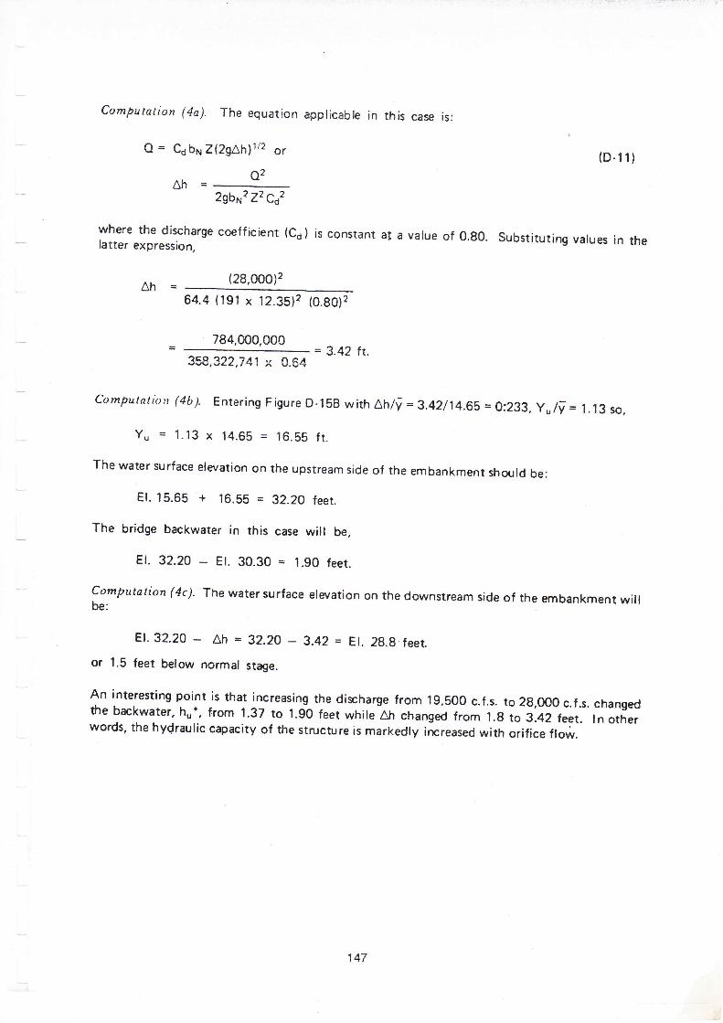
Computation (4a). The equation applicable in this case is:
Q = CobrvZt2gAh) 1t2 ortD-11)
Ah=O'2gbn,2 22 coz
where the discharge coefficient (c6) is constant aI a value of 0.80. substituting values in thelatter expression,
ah _ (28,000)2
64.4 (191 x 12.35)2 (O.go)2
784,000,000= 3.42 tt.
358,322,74't x 0.64
Computation (4b). Entering Figure D-158 with Ah/t = 3.42/14.65 = 0:233, yu/i = 1.13 so,
Yu = 1.13 x 14.65 = 16.55 ft.
The water surface elevation on the upstream side of the embankment shotrld be:
El. 15.65 + 16.55 = 32.20 feet.
The bridge backwater in this case will be,
El. 32.20 - Et. 30.30 = 1.90 feet.
computation (4c)' The watersurface elwation on the downstream side of the embanknnent willbe:
El. 32.20 - Ah = 32.20 _ 3.42 = Et. 2g.g feet.
or 1.5 feet below normal stage.
An interesting pointis that increasing the discharge from 1g,500 c.f.s. to2g,o00c.f.s. changedthe backwater, hr*, from 1.37 to 1.90 feet while Ah changed from l.g to 3.42 feet. ln otherwords, the hydraulic capacity of the structure is markedly increased with orifice flow.
147

ACKNOWLEDGEMENTS
TECHNICAL COMMITTEE 6 - DRAINAGE
Main Cornmittee Merntrers
Nafisah Hj. Abdul Aziz
Ahmad Fuad Emby
Wan Suraya Mustaffa
Normala Hassan
Teh Ming Hu
Lim Kim Oum
Alias Hashim
Low Kom Sing
Nor Asiah Othman
Johan Les Hare Abdullah
Chairman
Deputy Chairman
Secretary
Alternate Secretary
Committee member
Committee member
Committee member
Committee member
Committee member
Editor
Sub'Committee Members for Volume 3 - Hydraulic Considerations in BridgeDesign
Lim Kim Oum
Normala Hassan
Yeap Chin Seong
Chin Kok Hee
K. Nanthakumar
Chia Chong Wing
Ng Kim Hooi
Chairman
Secretary
Committee member
Committee member
Committee member
Committee member
Committee member

ACKNOWI,EDGEMENTS
Volume 3 is not part of the Arahan Teknik (Jalan) f5197 - INTERMEDIATE GUIDETO DRAINAGE DESIGN OF ROADS. Technical Committee 6 felt that there is aneed to provide guidelines for the hydraulic aspects in bridge design.
Volume 3 provides guidelines for the practical aspects of bridge hydraulic design.The more theoretical considerations and design worked examples are provided inAppendix 1, which is reprinted from Jabatan Pengairan dan Saliran publication -Urban Drainage Design Standards and Procedures for Peninsular Malaysia (1975),Appendix D - Hydraulic Design of Bridges.
Thanks are due to:
Jabatan Pengairan dan Saliran for permission to reprint Urban DrainageDesign Standards and Procedures for Peninsular Malaysia (7915), AppendixD - Hydraulic Design of Bridges"
REAM Standing Committee on Technology and Road Management for theguidance and encouragement given in the preparation of Voiume 3"
Members of the Technical Committee 6 - Drainage and Sub-Committee forHydraulic Considerations in Bridge Design for their untiring efforts to ensuretimely completion of Volume 3.