Recent developments in the ABINIT software package

X. Gonzea,b, F. Jollet?c, F. Abreu Araujoa, D. Adamsc, B. Amadonc, T.Applencourtc, C. Audouzec, J.-M. Beukena,b, J. Biederc, A. Bokhanchukk,l, E.Bousquete, F. Brunevalf, D. Calisteg, M. Coteh, F. Dahmc, F. Da Pievea,b, M.

Delaveauc, M. Di Gennaroe,b, B. Doradoc, C. Espejow, G. Genestec, L.Genoveseg, A. Gerossierc, M. Giantomassia,b, Y. Gilleta,b, D. R. Hamannp,q,L. Hem,n, G. Jomardr, J. Laflamme Janssena,b, S. Le Rouxa,b, A. Levittc, A.

Lherbiera,b, F. Liuo, I. Lukacevicu, A. Martinc, C. Martinsc, M. J. T.Oliveiraj,b, S. Poncea,b, Y. Pouilloni, T. Rangelc, G.-M. Rignanesea,b, A. H.

Romerov, B. Rousseauh, O. Rubelt, A. A. Shukrif, M. Stankovskis, M.Torrentc, M.J. Van Settena,b, B. Van Troeyea,b, M. J. Verstraetee,b, D.

Waroquiera,b, J. Wiktorr, B Xue,b, A. Zhoum, J. W. Zwanzigerd

aUniversite Catholique de Louvain, Louvain-la-Neuve (Belgium)bEuropean Theoretical Spectroscopy Facility (ETSF)

cCEA DAM-DIF, F-91297 Arpajon, FrancedDepartment of Chemistry and Institute for Research in Materials, Dalhousie University,

Halifax, CanadaeQ-Mat,Department of Physics, University of Liege (Belgium)

fCEA, DEN, Service de Recherches de Metallurgie Physique, F-91191 Gif-sur Yvette,France

gLaboratoire de Simulation Atomistique (L Sim), SP2M, UMR-E CEA/UJF-Grenoble 1,INAC, Grenoble, F-38054, France

hPhysics Department, University of Montreal, Montreal, CanadaiEuskal Herriko Unibertsitatea & Materials Evolution, Donostia-San Sebastian, SpainjCFisUC, Department of Physics, University of Coimbra, 3004-516 Coimbra, PortugalkThunder Bay Regional Research Institute, 980 Oliver Road, Thunder Bay, Ontario,

CanadalConfederation College, 1450 Nakina Dr., Thunder Bay, Ontario, Canada

mLSEC, Institute of Computational Mathematics and Scientific/Engineering Computing,Academy of Mathematics and Systems Science, Chinese Academy of Sciences, Beijing

100190, ChinanSupercomputing Center, Computer Network Information Center, Chinese Academy of

Sciences, Beijing 100190, China.oSchool of Statistics and Mathematics, Central University of Finance and Economics,

Beijing 100081, ChinapDepartment of Physics and Astronomy, Rutgers University, Piscataway, NJ 08854-8019

qMat-Sim Research LLC, P. O. Box 742, Murray Hill, NJ 07974rCEA, DEN, DEC, Centre de Cadarache, 13108, Saint-Paul-lez-Durance, France

sLund University,LU OPEN, Box 117, SE-221 00 LundtDepartment of Materials Science and Engineering,McMaster University, 1280 Main Street

West, Hamilton, Ontario, Canadau Department of Physics, University J. J. Strossmayer, Osijek, Croatia

vPhysics Department, West Virginia University, Morgantown, USAwDepartamento de Ciencias Basicas, Universidad Jorge Tadeo Lozano, Bogota, Colombia

Email address: francois.jollet@cea.fr (F. Jollet?)

Preprint submitted to Computer Physics Communications March 31, 2016

Abstract

ABINIT is a package whose main program allows one to find the total en-ergy, charge density, electronic structure and many other properties of systemsmade of electrons and nuclei, (molecules and periodic solids) within DensityFunctional Theory (DFT), Many-Body Perturbation Theory (GW approxima-tion and Bethe-Salpeter equation) and Dynmical Mean Field Theory (DMFT).ABINIT also allows to optimize the geometry according to the DFT forces andstresses, to perform molecular dynamics simulations using these forces, and togenerate dynamical matrices, Born effective charges and dielectric tensors.The present paper aims to describe the new capabilities of ABINIT that havebeen developed since 2009. It covers both physical and technical developmentsinside the ABINIT code, as well as developments provided within the ABINITpackage. The developments are described with relevant references, input vari-ables, tests and tutorials.

PACS: 70; 71.15.Mb; 78

Keywords: first-principles calculation, electronic structure, density functionaltheory, Many-Body perturbation theory

Program summaryProgram Title: ABINITJournal Reference:Catalogue identifier:Licensing provisions: GPL [1]Program summary URL: http://www.abinit.org/aboutProgramming language: Fortran2003, PERL scripts, Python scriptsDistribution format: tar.gzKeywords: first-principles calculation, electronic structure, density functional theory,Many-Body perturbation theoryPACS: 70; 71.15.-m; 77; 78Classification: 7.3 Electronic Structure, 7.8 Structure and lattice dynamicsExternal routines/libraries:(all optional) BigDFT [2], ETSF IO [3], libxc [4], NetCDF[5], MPI [6], Wannier90 [7], FFTW [8].

Nature of problem:This package has the purpose of computing accurately material and nanostructureproperties : electronic structure, bond lengths, bond angles, primitive cell size, co-hesive energy, dielectric properties, vibrational properties, elastic properties, opticalproperties, magnetic properties, non-linear couplings, electronic and vibrational life-times, and others.Solution method:Software application based on Density Functional Theory, Many-Body PerturbationTheory and Dynamical Mean Field Theory, pseudopotentials, with plane waves orwavelets as basis functions.References:[1] http://www.gnu.org/copyleft/gpl.txt

2

[2] http://bigdft.org

[3] http://www.etsf.eu/fileformats

[4] http://www.tddft.org/programs/octopus/wiki/index.php/Libxc

[5] http://www.unidata.ucar.edu/software/netcdf

[6] https://en.wikipedia.org/wiki/Message Passing Interface

[7] http://www.wannier.org

[8] M. Frigo and S.G. Johnson, Proceedings of the IEEE, 93, 216-231 (2005).

3

1. Introduction

The ABINIT software application allows one to compute many physicalproperties of systems made of electrons and nuclei (molecules and periodicsolids) thanks to a “first-principles” approach, i.e. without adjustable param-eters. The ground state properties are calculated in the frame of the Density-Functional Theory (DFT) as proposed by Hohenberg and Kohn [1] and Kohnand Sham [2], using many different exchange correlation (XC) functionals, whereasthe GW approximation (GW) proposed by Hedin [3] and Bethe-Salpeter equa-tion [4] can be used for excited states. Generally speaking, for solids and systemsstructured at the nanoscale, even weakly bonded, these give access to cohesiveproperties, geometry predictions, vibrational, magnetic, elastic, thermodynam-ical, thermoelectric and dielectric properties, electronic structure, optical prop-erties, spectroscopic responses, and several non-linear properties of solids.

The ABINIT project started in 1997 and the first publicly available versionof ABINIT was released in December 2000 under the GNU GPL [5]. It hasalready been described in 2002 [6], 2005 [7] and 2009 [8]. The last stable versionof the package (7.10.5) occupies about 70 MBytes, and gathers nearly 1400 fileswritten in F90 (830000 lines), including documentation, tutorials and more thanone thousand tests. The code is developed by an open community (around fiftypeople) and it is used by more than a thousand researchers worldwide. A Website [9] provides the latest version of the package, the on-line documentationand many entry points for the tutorial [10]. A forum is available for questionswith many different topics and all levels of complexity [11] and a wiki has beenrecently developed [12] to house documentation and FAQ extracted from theforum.

The capabilities of ABINIT have been described in detail in the last generalpaper on ABINIT published in 2009 [8]. The aim of this new paper is to describethe new capabilities than have been developed since that time :

• Section 2 is devoted to a brief summary of the evolution of ABINIT con-cerning the structure of the package, and how to run the code.

• In section 3, we shall detail the new physical features developed in the codethese last 6 years. We focus on major developments and only briefly men-tion the other ones. Major developments include quantum effects for thenuclei treated by the Path-integral Molecular Dynamics, finding transitionstates using image dynamics (NEB or string methods), some developmentsmade in the ground state calculations (finite electric fields and two com-ponent DFT for electron-positron annihilation), developments made inlinear and non-linear responses (linear response in a Projector Augmented-Wave approach -PAW-, electron-phonon interactions and temperature de-pendence of the gap), developments made in excited state calculations(Bethe Salpeter Equation -BSE-) and the Dynamical Mean Field Theory(DMFT).

• In section 4, recently developed technical features will be described, par-ticularly the advances concerning the development of a PAW approach for

4

a wavelet basis, the parallelisation of the code and the build system.

• Other developments concerning the ABINIT package will be presented insection 5, especially those which concern the tests, the test farm, the tuto-rials, pseudopotentials and PAW atomic data, the GUI and postprocessingtools like the AbiPy and APPA libraries or the supercell unfolding.

• Finally, on-going developments, which will be included in the next versionof the package, will be briefly presented in section 6. These include aninterpolation technique for the BSE calculations, the availability of hy-brid DFT and Van der Waals functionals, a new G0W0 implementation,the DFPT computation of effective masses and improvements related toRPA dielectric susceptibility calculations (electro-optic effect and secondharmonic generation with anti-resonant contributions and/or scissor cor-rection).

In each section, a brief presentation of the underlying theory of the new fea-ture will be given, followed by the input variables for activation and references,tests, and tutorials if any. Tests are specified by the subdirectory of tests/ inwhich they reside and the number of the test, e.g., v7#80.

5

2. Overview of ABINIT

2.1. Structure of the main ABINIT program, and other main programs

From the user’s perspective, the main ABINIT program, abinit the top-level routine of which is src/98 main/abinit.F90, is a “driver” attacking differ-ent “processing units”. This structure is unchanged with respect to ABINITv5.8,and is properly described in Ref. [8]. One important processing unit, the“Bether-Salpeter equation” that allows accurate computation of optical prop-erties and resonant Raman intensities, has been added, and will be describedin Sec. (3.5.1). The other ones (ground state calculations, including geometryoptimization ; linear responses ; non-linear responses ; GW computations) areoperational, with added capabilities with respect to ABINITv5.8.

The sources of the different F90 programs of the ABINIT package are presentin the src/ directory. Compared to ABINITv5.8, the src/ directory has beenrestructured. Most of the subdirectories names now start with a two-digit radix,from 01 to 98, followed by an underscore. Source files in one such subdirectorycan only rely on source files in the same directory or from a directory with a lowertwo-digit characteristics. In particular, the top-level routines, for independentexecutables (not only abinit), are contained in src/98 main.

The set of major executables in src/98 main is also unchanged with respectto ABINITv5.8 (abinit, anaddb, cut3d, conducti, optics, ujdet), althoughsome post processors, or conversion tools, that had become obsolete due toother developments, or lack of maintenance, have been removed (abinetcdf,compare interpol, lwf). Also, utilities have been added :src/98 main/bsepostproc.F90 for the post-processing of BSE results,src/98 main/kss2wfk.F90 for the conversion of KSS files to WFK files. Somenew profiling tools are present as well, src/98 main/fftprof.F90,src/98 main/ioprof.F90, and src/98 main/lapackprof.F90. A Van der Waals“DF” type of computation can be prepared by generating the kernel withsrc/98 main/vdwkernelgen.F90, see Sec. (6.4).

2.2. Structure of the package

During the last seven years, there has been a steady move towards a moremodular structure of the ABINIT package. The motivation and main ideashave been explained in Ref. [8], with noticeable changes for specific directories.Although the src/ directory still contains the source code (with however its ownbuild system), the so-called “plug-ins” and “prerequisites” have been supersededby “fallbacks”, fallbacks/, with the change of philosophy that the mandatorycomponents (BLAS, LAPACK) should not be shipped by default with ABINITpackage, but the user should use the best compiled libraries available on his/hercomputer for the execution of the computations. Among the optional externallibraries of ABINIT, only FoX has been replaced by PSML, while for the others(BigDFT, NetCDF, ETSF IO, LibXC, Wannier90), rather recent versions areinterfaced with ABINIT. The tests/ directory has been split in two directories,the tests of capabilities of ABINIT being kept in tests/, while the tests offulfillment of coding rules, memory leaks, documentation of variables, etc, (see

6

Sec. 5.1) have been moved to the directory special/. The directories utils/

and extras/, have been suppressed, and their content (with additional files) hasbeen restructured in the two new directories developers/ and scripts/. Thedirectory developers/ contains tools, scripts and miscellaneous information fordevelopers. Scripts that might be useful for the users are contained in scripts/.Finally, the additional directories coverage/, packages/ and watch/ are usefulfor developers only.

In recent years, a separate Python package has been developed for the man-agement and post processing of the output of ABINIT, called AbiPy. Althoughnot part of the ABINIT package, it is intimately linked to ABINIT, and it isdescribed in this document as well. It is especially useful in the context of high-throughput calculations. Also, AbinitGUI, a GUI for ABINIT, written in Java,allows one to launch and manage ABINIT runs, and has numerous capabilitiesto help beginners set up ABINIT runs and analyze their output. This projectis described in Sec. 5.4.3. In view of their size and post- or pre-processingcharacteristics with respect to the ABINIT package, it has been chosen not tomake them part of the main ABINIT package (as it is itself already quite large).

2.3. How to build and run ABINIT

The steps hereafter apply to the build and run of ABINIT under Linux, inthe simple case where the mandatory libraries (BLAS, LAPACK) are installedalready. ABINIT will also try to determine whether other (optional) librariesare available. If these simple instructions fail, or if the user wants more controlon the build of ABINIT, one should refer to the installation notes and helpfiles, that are available on the ABINIT Web site, or in the doc directory ofthe package. Also, compilation/build help can be found on the ABINIT forumhttp://forum.abinit.org/.

First step : download, gunzip and untar the ABINIT package from theABINIT Web site (or from the CPC site), then change the current directory tothe top of the directory that was created.

gunzip abinit-7.10.5.tar.gz

tar -xvf abinit-7.10.5.tar

cd abinit-7.10.5

Second step : configure, make and (optionally) make install ABINIT, asfollows.

configure or ./configure

(or first create a tmp directory, then cd tmp, then ../configure)

make (or make mj4 , or make multi multi_nprocs=n for using ‘‘n’’

processors on a SMP machine where the user has to replace

‘‘n’’ by its value)

make install # optional

The last (optional) command will install abinit in the /usr/local directory,otherwise, it is available in src/98 main

7

Third step : run ABINIT, as follows, presuming the abinit executable is inthe path.

abinit < Filenames (or optionally abinit < Filenames > log)

where the content of the Filenames file is explained on the ABINIT Web site,or in the doc/users/abinit help.html file of the package.

New production versions of ABINIT will be made available as time goeson. We do not expect these build and run steps to be modified within thenext few years. Of course, for versions of ABINIT other than v7.10.5, the usershould change the package name abinit-7.10.5.tar.gz to the one of the newreleased package, like abinit-8.1.1.tar.gz, and modify the above-mentionedinstructions accordingly.

Ref. [8] contains more detailed explanations of the build of ABINITv5.8,most of which still apply. Replace “plugins” by “fallbacks”, and also note thatin v7.10.5, there is only a single main executable, named abinit, instead ofthe separate executable for the sequential and parallel cases, that were namedabinis and abinip in ABINITv5.8 . The latter change is actually the onlycommand line change to run ABINIT, as described in Sec. 2.5 of Ref. [8].

3. Recently developed physical features in ABINIT

3.1. Path-Integral Molecular Dynamics

Path-Integral Molecular Dynamics (PIMD) is a technique allowing to simu-late the quantum fluctuations of the nuclei at thermodynamic equilibrium [13].It is implemented in ABINIT in the NVT ensemble since v7.8.2.

In the Path-Integral formalism of quantum statistical mechanics, the (quan-tum) nuclei are replaced by a set of images (beads) treated by means of classicalmechanics, and interacting with each other through a specific effective potential.In the limit of an infinite number of beads, the quantum system and this many-beads classicle system have the same partition function, and thus the same staticobservables. In PIMD, the classical system of beads is simulated by standardMolecular Dynamics. The PIMD equations of motion are integrated by usingthe Verlet algorithm. At each time step, a ground state DFT calculation is per-formed for each image. PIMD can be used with any XC functional and works inthe PAW framework as well as in the norm-conserving pseudopotential (NCPP)case.

PIMD in ABINIT follows the set of numerical schemes developed by severalauthors in the 90’s [13, 14]. PIMD in the canonical ensemble needs specificthermostats to ensure that the trajectories are ergodic: the Nose-Hoover chainsare implemented, as well as the Langevin thermostat (controlled by the valueof imgmov). Also, it is possible to use coordinate transformations (stagingand normal mode), that are controlled by the keyword pitransform. In stan-dard equilibrium PIMD, only static observables are relevant (quantum time-correlation functions are not accessible): the masses associated to the motionof the beads are controlled by the keyword pimass, whereas the true masses of

8

the atoms are given by amu. The values given in pimass are used to fix theso-called fictitious masses [13]. In the case where a coordinate transformation isused, the fictitious masses are automatically fixed in the code to match the so-called staging masses or normal mode masses. The number of time steps of thetrajectory is controlled by ntimimage, the initial and thermostat temperatureby mdtemp(2). Except if specified, the images in the initial configuration areassumed to be at the same position, and a random distribution of velocities isapplied (governed by mdtemp(1)) to start the dynamics.

At each time step, ABINIT delivers in the output file:(i) information about the ground state DFT calculation of the ground state foreach image(ii) the instantaneous temperature, the instantaneous energy as given by theprimitive and virial estimators, and the pressure tensor as given by the primitiveestimator.An automatic test is given with the code (v7#08) and a tutorial will be providedin a next version of the package.

PIMD in ABINIT enters a larger family of algorithms that use images of thesystem (controlled by the keyword imgmov), such as the String method or theNudged Elastic Band method, both described in the next section (Sec. 3.2). Thenumber of images (keyword nimage) is associated to a specific parallelizationlevel (keyword npimage).

PIMD has been used with ABINIT to reproduce the large isotope effect onthe phase transition between phase I and phase II of dense hydrogen [15], andalso some aspects of diffusion at low and room temperature in proton-conductingoxides for fuel cells [16]. PIMD in the NPT ensemble is not available yet.

3.2. Transition states from image algorithms

Similarly to the PIMD, finding minimum energy paths and in particulartransition states for chemical transformations is of great importance in manydifferent fields. In ABINIT we have implemented two different flavours based oninterpolation methods [17, 18, 19] and controlled by the keyword imgmov. Thecalculation starts with the knowledge of the initial and final state (local minimain the configuration space) and an educated guess for the reaction pathway. Ifthe reaction path is not given, a linear interpolation between the reactants andfinal products is constructed by a series of images (configurations) that connectthe two states, which are given by the keyword nimage. The energy path thatjoins the series of images is then modified at each step to allow the search overthe lowest energy path joining the reactants and products.

In the Nudge Elastic Band method (NEB), the images are connected throughsprings, with a spring constant that has to be chosen such that the images areuniformly spaced during the path search. The forces on each image come fromthe potential energy surface of that configuration and a spring force from thetwo closest configurations. The change in images is calculated by projectingout the true force perpendicular to the path and the parallel projection of thespring force with respect to the path [18]. The spring constant is obtained from

9

the keyword neb spring and the number of iterations is given by ntimim-age. In the String method, the system set up is exactly the same as in theNEBM with the difference that no spring constant needs to be defined. In thiscase, the forces are obtained as in the NEB method from the true force perpen-dicular but now the configurations are equally redistributed along the path ateach iteration [17]. In both methods, the search stops if the number of prede-fined iterations (ntimimage) or the tolerance convergence criteria (tolimg) isreached.

As in the PIMD, each of the images can be treated in parallel and the re-quested parallelization mode is set with the keyword npimage. Automatic testsfor the string method are provided: paral#08, tutoparal#03 and tutoparal#4,v6#24, v6#25. Moreover a tutorial for the use of the string method in parallelis available (see [10] or doc/tutorial/lesson parall string.html).

3.3. Developments in ground state calculations

3.3.1. Finite Electric field

The effect of an homogeneous static electric field on an insulator may betreated in ABINIT from two perspectives. One is perturbative, and yields thesusceptibility in the form of the second derivative of the total energy with re-spect to the electric field, at zero field strength. This approach is discussedbelow in Section 3.4.1. ABINIT can also be used to compute the effect of anelectric field of finite amplitude, using techniques from the Modern Theory ofPolarization [20, 21, 22]. In this approach, the total energy to minimize in-cludes the contribution due to the interaction of the external electric field withthe material polarization PTot, as follows:

E = E0 − ΩPTot ·E, (1)

where E0 is the usual ground state energy obtained from Kohn-Sham DFT inthe absence of the external field E, PTot is the polarization, made up of an ioniccontribution and an electronic contribution, and Ω the volume of the unit cell.The Modern Theory of Polarization provides a formula for the electronic partPel as

Pel · bi =fe

Ω

1

N i⊥

Ni⊥∑

Im ln

Ni‖∏

detMki,ki+∆ki . (2)

where f is the spin degeneracy and e the charge (-1 for electrons). Here the com-ponent of Pel in direction bi of the reciprocal lattice is computed, by discretizinga line integral through the Brillouin zone in the bi direction and summing overpoints in the plane perpendicular to this line. The integrand, which is the Berryconnection, is discretized in terms of the matrix Mki,ki+∆ki [23], with matrixelements

Mki,ki+∆kimn = 〈umki

|unki+∆ki〉, (3)

that is, the overlap of Bloch states umkiat neighboring k-points along the

integration path.

10

In ABINIT, the polarization of the ground state may be computed usingEq. 2, and the effect of an external electric field is included by minimizing thetotal energy in Eq. 1. The latter case proceeds as usual by expressing theenergy in terms of matrix elements of the Kohn-Sham Hamiltonian (and thepolarization term), and functionally differentiating with respect to the bra ofinterest 〈umki

|. The discretized form in Eq. 2 is handled by use of the matrixidentity d(ln detM)/dλ = Tr(M−1dM/dλ). Either the NCPP or the PAWscheme may be used [24]. In the case of PAW, the matrix elements of Eq. 3have contributions from both the planewave expansion of the Bloch functionsand from the atom-centered projectors, as follows:

〈umki|unki+∆ki

〉 = 〈umki|unki+∆ki

〉+ (4)∑qrI

〈umki|pIqki〉QIqr(∆ki)〈pIrki+∆ki

|unki+∆ki〉,

where the sum runs over ions, labeled by I, and atomic-like orbitals ϕIq on eachion labeled by q, the p are the PAW projectors, umki

the pseudized Bloch states,and

QIqr(∆ki) = e−iI·∆ki

[〈ϕIq |e−i∆ki·(r−I)|ϕIr〉 − 〈ϕIq |e−i∆ki·(r−I)|ϕIr〉

](5)

is the on-site PAW contribution to the overlap of states at adjacent k-points. Ex-pansion of Q in terms of ∆k leads to a first-order contribution that is effectivelyan on-site dipole moment, as identified already in the ultra-soft pseudopotentialtreatment of polarization [25]. However the exponential in Q can be treated ex-actly to all orders in Eq. 4, in which case the dipole should not be additionallyincluded (as it erroneously was in Ref. [24]). In ABINIT the exact treatment isused, and the dipole is also reported for reference.

In the NCPP case, the electric field has no additional contribution to theHellmann-Feynman forces, because the electronic states do not depend explicitlyon ionic position [22]. In the PAW case however, as the projectors do dependon ion location, an additional force term arises when Eq. 2 is differentiatedwith respect to ion position, and similarly for stress [24]. The same identitymentioned above is used to differentiate ln detM with respect to ion position orstrain.

The polarization and finite electric field calculation in ABINIT is accessedthrough the variables berryopt and efield. In addition, displacement fieldsand mixed boundary conditions (a mix of electric field and displacement field)can be computed as well. A tutorial is also provided for these calculations (see[10] or doc/tutorial/lesson ffield.html).

3.3.2. Two component Density Functional Theory: electron-positron annihila-tion

Two-component density functional theory (TCDFT) [26, 27, 28] is a gener-alization of the density functional theory, which allows one to determine densi-ties and wavefunctions of interacting positrons and electrons. These quantities,

11

in turn, can be used to model two positron annihilation characteristics, thelifetime of a positron and the momentum distribution of annihilating electron-positron pairs (Doppler broadening), which are measured in positron annihila-tion spectroscopy (PAS) [29]. Numerous coupled experimental and theoreticalpositron annihilation studies [30, 31, 32, 33, 34, 35] on defects in solids provethe importance of first principles calculations for defect identification. A fullyself-consistent TCDFT scheme along with the positron lifetime calculations hasbeen implemented in ABINIT in the PAW [36] framework since v6.0.1. Methodsfor Doppler broadening of the annihilation radiation calculations are availablesince v7.10.1. The implementation is described in detail in Ref. [37].

The TCDFT is implemented as a double loop on the electronic and positronicdensities: during each subloop, one of the two densities (and Hamiltonians) iskept constant while the other is being converged. There are two ways of perform-ing positron calculations: In the first, manual, way, one needs to perform elec-tronic ground-state calculation (positron=0), then a positronic ground-statecalculation (positron=1) with the electronic density automatically read froma DEN file, followed by an electronic calculation in the presence of the positron(positron=2). The second and the third steps can be then repeated. Theprocedure can be also performed automatically using positron=-1 (electronicand positronic wavefunctions not stored in memory), positron=-10 (electronicand positronic wavefunctions stored in memory). The convergence of the to-tal energy (resp. the forces) for the positrons is controlled by the use of thepostoldfe (resp. postoldff) and posnstep input keywords.

Forces and stresses, including contributions from the electrons and the positron,can be evaluated, and the calculation continued with a new atomic configurationand/or new geometry. In this implementation we use a unified formalism for thepositron and the electrons: the wavefunctions of the electrons and the positronin the system are expressed on the same mixed basis (plane-waves and atomicorbitals). Thanks to this, we can use the same PAW datasets for electronsand positron. The PAW datasets, however, are originally generated to describeelectronic wavefunctions and not the positronic ones. Because of the nature ofthe electron-ion and positron-ion interactions, the shapes of the correspondingwavefunctions differ strongly. Therefore, in some cases, a standard PAW datasetcan be inappropriate for the positron description. Two ways of overcoming thisproblem are proposed [37]: First, the number of valence electrons in the PAWdataset can be increased. The second, less time consuming solution, is to addthe partial waves corresponding to the semicore electrons in the basis used forthe positron wavefunction description, while keeping the initial number of va-lence electrons. The PAW datasets can be generated using a modified versionof the ATOMPAW generator [38].

Several electron-positron correlation functionals, including LDA and GGAzero-positron density limit and LDA full electron-positron correlation functional,are available and are controlled by the keyword ixpositron.

At the end of each positron calculation, a positron lifetime (decomposed inseveral contributions) is printed. In order to output the momentum distributionsof annihilating electron-positron pairs the posdoppler keyword should be set

12

to 1. The three-dimensional momentum distributions can be then projectedin various directions, giving Doppler spectra for comparison with experiments,using the posdopspectra script in the scripts/post processing directory.An automatic test is given with the code (v7#35).

The TCDFT calculations have been parallelized on three levels, allowing oneto use the Locally Optimal Block Preconditioned Conjugate Gradient (LOBPCG)[39] or the Chebyshev filtering algorithm [40]. This means that the processorscan be distributed between the k-points, bands and FFT grid points during thedensity, lifetime and momentum distribution calculations.

The TCDFT implementation in ABINIT has been used to contribute toidentify defects in SiC [41, 42, 34] and UO2 [35].

3.3.3. Other ground state developments

Kinetic energy densityThe computation of the kinetic energy density

τ(r) =1

2

∑k

∑n

f(Enk)|∇ψnk(r)|2 (6)

where f(Enk) is the occupation number of the eigenstate ψnk(r), has beenimplemented in the ABINIT software from version 6 for the norm-conservingpseudopotential case. An implementation for the PAW case will become avail-able in a future release of the code. The kinetic energy density is computed ifthe keyword usekden is set to 1. The kinetic energy density is mainly usefulin two places in the code. It is used in the calculation of the electron localiza-tion function (ELF), and can also be required when using meta-GGA (MGGA)functionals.

ELFThe ELF[43, 44] gives a dimensionless measure of the electron pairing proba-bility, that is the probability of finding an electron in the vicinity of anotherreference electron. Similarly to the Atoms in Molecules (AIM) method[45], theELF is mainly used in quantum chemical topology analysis to scrutinize thechemical bonding. The electron localization function is defined as

ELF(r) =1

1 +(

D(r)D0(r)

)2 (7)

and falls in the range [0,1]. The ELF is equal to 1 for perfect localization andELF=1/2 when the Pauli kinetic energy density

D(r) = τ(r)− 1

8

|∇n(r)|2

n(r)(8)

becomes equivalent to that of a homogeneous electron gas

D0(r) =3

10(3π2)2/3n5/3(r) (9)

13

Using the keyword prtelf, the ELF can be output in a ELF file which canbe post processed and analyzed similarly to the DEN file which contains theelectronic density.

The LibXC library and Meta-GGA functionsThe Libxc project [46] provides an implementation of almost all published

exchange-correlation functionals, in a well tested, robust library which is re-leased under the GNU Lesser General Public License (version 3.0). It is writtenin C, and includes bindings for Fortran.

In ABINIT, starting from version 5.7, it became possible to use Libxc toobtain the exchange-correlation energy Exc and potential vxc within LDA andGGA. It is now also possible to use it also within MGGA and for hybrid func-tionals (see section 6.3 for the latter).

The MGGA functionals come as the third rung of the Jacob’s ladder of DFTafter LDA and GGA. The functionals from this family have an added depen-dence on either the kinetic energy density (τ) or the laplacian of the electronicdensity (∇2n), or both. This means that τ and ∇2n are required in the calcula-tion of the MGGA exchange-correlation energy Exc. The calculations of τ and∇2n are interfaced with Libxc such that many MGGA functionals are availablein ABINIT. Automatic tests of the implementation are provided from v6#31to v6#33, and the corresponding documentation can be found in the directorydoc/theory/MGGA. However, the present implementation does not yet includean adaptated mixing procedure in the self-consistent-field cycles. Therefore,only a restricted list of MGGA is currently available. We recommend to theMGGA-users to employ the Vxc-only MGGA based on an LDA correlation part(typically ixc -207012, -208012, and -209012), and not those which allow totalenergy calculations (and the associated computation of forces). Consequently,structural optimization is not yet possible within a full MGGA approach. Theuse of MGGA functionals is expected to yield a better accuracy on ground statepredictions although this can depend strongly on the chosen functional. As anexample, it has been demonstrated that the TB09 MGGA functional allows abetter prediction of the electronic band gaps [47]. However, it is worth notingthat in this particular case this might be at the price of a worse band width andthus a worse description of the effective masses [48].

External magnetic fieldAn applied external magnetic field has been implemented in ABINIT by consid-ering the Zeeman spin response only (i.e., neglecting the orbital contribution).Following the procedure of Bousquet et al.,[49] the applied B field is introducedby adding the following term in the non-collinear Kohn-Sham potential:

VZeeman = −g2µB

(Bz Bx + iBy

Bx − iBy −Bz

)(10)

where g is the Lande factor for the spins, µB the Bohr magneton and Bi thecomponent of the B-field along i =x, y and z directions. This contributionis trivial to implement, and also dominant in amplitude, but has historicallybeen neglected with respect to the orbital responses, which are rich in more

14

complex physics. Unlike an applied electric field, such a Zeeman term in thepotential is compatible with periodic boundary conditions. It is also compatiblewith collinear calculations by reducing its application on “up” and “down” spinchannels with B=B~ez. In ABINIT, the finite Zeeman field is controlled by thekeyword zeemanfield which allows to control the amplitude of the applied B-field (in Tesla) along the three cartesian directions. Such an applied Zeeman fieldallows one to calculate the spin contribution of the magnetic and magnetoelectricsusceptibilities, and to observe phase transitions under finite magnetic field, ifpresent. The automatic test v6#17 shows an example of an applied Zeemanmagnetic field on an isolated Bi atom.

Constrained atomic magnetic momentsA complementary magnetic constraint method has been implemented in theABINIT code, wherein the magnetization around each atom is pushed to a de-sired (vectorial) value. The constraint can either be on the full vector quantity,

~m, or only on the direction ~m. This is mainly useful for non collinear systems,where the direction and amplitude of the magnetic moment can change. Themethod follows that used in the Quantum Espresso [50] and VASP [51] codes:a Lagrangian constraint is applied to the energy, and works through a result-ing term in the potential, which acts on the different spin components. Themagnetization in a sphere Ωi around atom i at position ~Ri is calculated as:

~m =

∫Ωi

~m(~r)d~r (11)

and the corresponding potential for spin component α is written as:

Vα = 2λf(|~r − ~Ri|/rs)~cα (12)

The function f(x) = x2(3+x(1+x(−6+3x))), is applied to smooth the transition

near the edge of the sphere around ~Ri, over a thickness rs (by default 0.05 bohr,

and f is set to 0 for |~r − ~Ri| > rs). This minimizes discontinuous variations ofthe potential from iteration to iteration.

The constraint is managed by the keyword magconon. Value 1 gives aconstraint on the direction (~c = ~m− ~si(~si · ~m)), value 2 gives a full constraint onthe vector (~c = ~m− ~si), with respect to the keyword spinat (~si above), givinga 3-vector for each atom. The latter is quite a stringent constraint, and oftenmay not converge. The former value usually works, provided sufficient precisionis given for the calculation of the magnetic moment (kinetic energy cutoff inparticular).

The strength of the constraint is given by the keyword magcon lambda(λ above - real valued). Typical values are 10−2 but vary strongly with systemtype: this value should be started small (here the constraint may not be enforcedfully) and increased. A too large value leads to oscillations of the magnetization(the equivalent of charge sloshing) which do not converge. A correspondingLagrange penalty term is added to the total energy, and is printed to the logfile, along with the effective magnetic field being applied. In an ideal case

15

the energy penalty term should go to 0 (the constraint is fully satisfied). Theautomatic test v7#05 runs different types of constraint combinations, for BCCiron.

Charged cellsIt is well known that the electrostatic potential (arising from ion-ion, ion-

electron, and electron-electron interactions) is ill-defined within periodic bound-ary conditions. However, it is less well known that the total energy of a chargedcell is also ill-defined. In fact, after a careful derivation in Ref. [52], it was shownthat the above two statements are tightly linked: when the number of electronsdiffers from the number of protons in a cell, the necessary compensating back-ground that enforces the overall charge neutrality is sensitive to the arbitraryaverage electrostatic potential.

ABINITv7.10 offers the possibility to choose which convention to use for theaverage electrostatic potential with the keyword usepotzero. In PAW, one canchoose among 3 options:

• the average of smooth electrostatic potential is set to zero;

• the average of all-electron electrostatic potential is set to zero;

• the average of smooth electrostatic potential is set to a finite value, whichfollows the Quantum Espresso implementation (see ref. [53] for moredetails).

Only options 1 and 3 are valid for the NCPP case.None of these conventions is intrinsically more correct than the other ones.

This is just an arbitrary choice, but ABINIT now permits a straight comparisonto the other codes.

3.4. Developments in linear and non-linear responses

3.4.1. Projector Augmented-Wave approach to Density-Functional PerturbationTheory

Density-Functional Perturbation Theory (DFPT) allows one to address alarge variety of physical observables. Many properties of interest can be com-puted directly from the derivatives of the energy, without the use of finite dif-ferences: phonons modes, elastic tensors, effective charges, dielectric tensors,etc. Such DFPT capabilities have been implemented for years in ABINIT inthe NCPP scheme [54, 55], but they were not available in the framework of thePAW approach.

From version 6, linear responses started to be implemented within PAW.They can almost all be used in the current production version of ABINIT 7.10.The few missing mixed responses will be available with version 8.

Prior to implementation, it was necessary to derive the theoretical formal-ism [56, 57]. Compared to NCCP, the equations become more complex becauseof: (1) the PAW “on-site” contributions, (2) the non-orthogonality of the pseudowave-functions, (3) the introduction of a compensation charge density. A PAW-DFPT calculation workflow is similar to that of a NCPP calculation, exceptthat one uses a PAW atomic dataset, and is conducted as follows:

16

• Run a Ground-State calculation in order to extract the Kohn-Sham pseudowave-functions ψn; these must be extremely well converged.

• If necessary, e.g., for the application of the derivative of the Hamiltonianwith respect to an electric field, determine the derivatives of the wavefunctions with respect to the wave vector k, and keep them in a file. Thekeyword rfddk is used to perform this type of calculation.

• Compute the 2nd-order derivative matrix (i.e., 2nd derivatives of the en-ergy with respect to different perturbations λ). This can be done thanksto the keywords rfphon (λ=atomic displacement), rfstr (λ=strain) orrfelfd (λ=electric field). This calculation is performed in 3 steps withABINIT:

1. compute the constant-wavefunctions term,

2. Determine the derivatives of the wavefunctions by solving the Stern-heimer equation. In the PAW approach, handling non-orthogonalpseudo wavefunctions, this equation, and the associated orthogonal-ity condition (in the parallel-transport gauge), are:

P ∗c (H− εnS)Pc|∂ψn∂λ〉 = −P ∗c

(∂H∂λ− εn

∂S∂λ

)|ψn〉 (13)

〈∂ψn∂λ|S|ψn〉 = −1

2〈ψn|

∂S∂λ|ψn〉 (14)

H (resp. S) is the Hamiltonian (resp. Overlap) operator. Pc is theprojector defined as Pc = 1−

∑n |ψn〉〈ψn|S.

3. Mix the wavefunction derivatives with the (non self-consistent) deriva-tives of the Hamiltonian to compute the complete derivative database.

• Launch the anaddb tool (distributed with ABINIT) to analyse the deriva-tive database and compute relaxed tensors and thermodynamical proper-ties.

Running a DFPT calculation within PAW requires no other additional pa-rameter than using a PAW atomic dataset (available on the web site thanksto the PAW JTH table, see 5.3.2) and adding — as for the ground-state, thepawecutdg keyword to tune the auxiliary fine grid. The parameter pawe-cutdg, should be converged even more carefully than in the ground state (bytesting the value of the desired response function) because it has a strong nu-merical impact on the second derivatives of the energy.

Note also that, when performing the post-processing with anaddb, it is rec-ommended to include all the keywords enforcing the sum rules (acoustic sumand charge neutrality). Indeed the PAW formalism involves, for each atom, thecalculation of a large number of real space integrals, whose numerical effect maybe to break the translational invariance.

17

With ABINIT 7.10, it it possible to access to the following response proper-ties with the PAW precision : (1) Phonon spectra for metals and insulators (in-cluding electric field contribution to LO-TO splitting), (2) dielectric tensor, (3)clamped-ion elastic tensor, (4) relaxed elastic tensor (including forces-internalstrain coupling coefficients) for metals. Other responses (effective charges andpiezoelectric tensor) are already planned for ABINIT v8, as well as some non-linear responses. anaddb then allows to compute many physical and thermody-namical properties containing derivatives of the energy.

Thanks to the locality provided by PAW partial wave basis, it is possible toperform response function calculations for correlated electron materials. TheLDA+U formalism is usable without any restriction for the PAW+DFPT calcu-lations.

Several automatic tests delivered in the package can be used as startingpoints to create input files for PAW-DFPT calculations: computation of wave-function derivatives with respect to k (v5#05), computation of dielectric tensor(v5#30), computation of phonons at several q vectors for insulators (v6#62,libxc#82) and metals (v6#89). All the tutorials dedicated to response functionscan be followed by substituting the NCPP files by PAW atomic datasets.

3.4.2. Electron-phonon coupling and transport

The calculation of electron-phonon coupling (EPC) quantities has been avail-able for over 10 years in the ABINIT code. These will be very briefly summa-rized, and new implementations described, which go beyond the elastic LowestOrder Variational Approximation (LOVA).

The calculation of transport quantities (for the normal and superconductingstates) dates back to Ziman [58] and before, but was pioneered in numericalapproaches by P.B. Allen [59, 60]. He applied an alternative method to therelaxation time approximation (RTA), based on an efficient basis set knownas Fermi Surface Harmonics (FSH). These are orthogonalized combinations ofpolynomials in the group velocity components ~vk, which form a complete basisfor the k variation of the electron phonon coupling. The strong advantage isthat, in the solution of the Boltzmann Transport Equations (BTE), only the 0thand 1st order terms appear explicitly in drift and diffusion. Thus, limiting thebasis set to the 1st order gives simple, closed, and relatively accurate forms forthe transport coefficients. The variational solution in the FSH basis gives thecurrent/electric field/conductivity which maximize the production of entropy.

For a full solution of the BTE, the basis set FSH are multiplied by functionsof the electronic energy σ(ε) (the dependency on k is thus double, through vkand εk). Here too, orthogonalized polynomial functions are used, and their ordern is limited to 0 and 1, which is enough to yield the conductivity and Seebeckcoefficients.

The formulae for the resistivity and electrical thermal conductivity are wellsummarized in the book by Grimvall [61]. Their implementation in an ab-initio/LMTO framework by Savrasov is the standard reference within DFT [62],yielding the Eliashberg spectral function α2F (ω) (with the related EPC coupling

18

strength and phonon linewidths), and its “transport” versions α2Ftr(ω) coinedby Allen.

Basic calculations of electron-phonon interaction in ABINIT have been re-viewed in previous papers, and are covered by an existing tutorial. One performsa normal ground state, then phonon calculations, with an added keyword prtgkk

which saves the matrix elements to files suffixed GKK. The main change in thisrespect is that prtgkk now disables the use of symmetry in reducing k-pointsand perturbations. This avoids ambiguities in wave function phases due to banddegeneracies. The resulting GKK files are merged using the mrggkk utility, andprocessed by anaddb if the flag elphflag is set to 1. With the implementationof phonons in PAW DFPT, the electron phonon coupling is also available inPAW, though this has not yet been tested extensively.

The LOVA approximation for transport was first used by Allen with an ad-ditional approximation, that of elastic processes, where the central EPC kernelis evaluated neglecting its electron energy variation (elastic LOVA; set ifltrans-port=1 in anaddb):

α2Ftr(s, s′;α, β; ε, ε′;ω) ' α2Ftr(s, s

′;α, β;ω) ' α2Ftr(1, 1;α, β;ω) (15)

where s, s′ = ±1 are akin to in/out scattering, ε, ε′ are electron energies (ifunspecified they are at the Fermi energy), ω is a phonon energy, and α, β arecartesian directions.

This is legitimate in simple metals, but will fail for more complex band struc-tures, such as narrow bands metals, or doped semiconductors with Fermi levelsnear to or in the band gap. Furthermore, the Seebeck coefficient (S) vanishesin the elastic LOVA as the asymmetry of electrons and holes is completely lost.

Going beyond the elastic LOVA (input variable ifltransport=2 for inelas-tic LOVA) can overcome the above-mentioned shortcomings, at the cost of sig-nificantly longer computation time and higher memory usage. The Seebecktensor is obtained from the ratio of two scattering operator matrix elements:Sαβ ≈ πkB√

3e

∑γ(Q01)αγ(Q11)−1

γβ , where the Q matrix is composed of the product

of the transport spectral function α2Ftr, the energy polynomials, and occupa-tion functions. The electron phonon scattering has been fully accounted forby fulfilling the conservation of energy and k′ − k = q + g with g a recipro-cal lattice vector. The sign and magnitude of S delicately relies on the energydependence of these quantities, such that relatively dense k- and q-meshes arenecessary. Note that only one fixed temperature is allowed per run, when settingifltransport to 2.

The LOVA Seebeck calculation overcomes the limitations of the often adoptedconstant RTA approach. A peculiar example has been studied in Ref. [63], wherethe unusual positive Seebeck of the simple alkali metal Lithium is well repro-duced and analyzed. By contrast, the constant RTA yields a negative sign ofS.

When the Fermi energy is near to or in the band gap, the (non constant)relaxation time approach is more appropriate. By setting ifltransport to 3,the fully ab initio k-dependent electron life time is computed, as in the work

19

of Restrepo[64] and others. It can be used to further calculate the electronictransport properties:

1

τk=

2π

h

∑q

|gk,k+q|2[f(εk+q) + nq

]δ(εk − εk+q + hωq)+

[1 + nq − f(εk+q)

]δ(εk − εk+q − hωq)

(16)

where g are the EPC matrix elements, f and n are the Fermi and Bose distribu-tions. Within this (non constant) RTA, the energy variation of the relaxationtime (weighted average over a uniform k-mesh) and mean free path (multipliedby the k-dependent velocities) are also calculated.

Other improvements include the consideration of the temperature depen-dence of the Fermi energy; cubic spline interpolation (ep nspline) to linearlyinterpolate the transport arrays and reduce the memory usage. Besides settingthe Fermi level with elph fermie (in Hartree), it is also possible to specifythe extra electrons per unit cell, (i.e., the doping concentration often expressedin cm−3) with ep extrael. New tests are found in v7#90 to #94 concernelectron-phonon calculations and transport for bcc Li.

3.4.3. Temperature dependence of the eigenenergies

The electronic structure changes with temperature. In most materials, suchchanges are mainly driven by the electron-phonon interaction, which is alsopresent at zero Kelvin, inducing the so-called zero-point motion renormaliza-tion (ZPR) of the eigenvalues. These effects can be computed thanks to theAllen-Heine-Cardona (AHC) theory [65, 66, 67], which is based on diagram-matic method of many-body perturbation theory. An extension to the standardAHC theory also gives access to the electronic lifetime and decay rates. Thesephysical properties are available from ABINIT since v7.10.4.

The ABINIT implementation of the AHC formalism relies on density-functionalperturbation theory (DFPT) [68, 54] and therefore allows for the calculation ofthe aforementioned quantities using the primitive cell only. It contains two mainapproximations: the harmonic approximation and the rigid-ion approximation(RIA). One can show that two Feynman diagrams are taken into account if theseapproximations are made: the Fan term (with two first-order electron-phononinteractions), and the Debye-Waller (with one second-order electron-phonon in-teraction). The impact of the electron-phonon coupling on the electronic eigen-state can be computed for semiconductors and insulators within an adiabaticor non-adiabatic framework. The AHC formalism and the implemented equa-tions can be found in Ref. [69]. An extended verification and validation study(also versus other first-principle codes) of the ABINIT implementation can befound in Ref. [70]. The AHC implementation can be used with any XC func-tional working with the response-function (RF) part of the code, and requiresthe use of norm-conserving pseudopotentials. NetCDF support is mandatory.In v7.10.4, only non-spin-polarized calculations are feasible (this constraint hasbeen removed in more recent version, see later).

20

The AHC implementation in ABINIT is built on a Sternheimer approach toefficiently compute the sum over highly energetic bands appearing in the AHCequations [71]. Such behavior is controlled by the input variable ieig2rf. Thek-point convergence can be strongly improved by restoring the charge neutralitythrough the reading of the Born effective charge and dielectric tensor (controlledby the input variable getddb). More information on the importance of chargeneutrality fulfillment can be found in Ref. [72]. The value of elph2 imagdensets the imaginary shifts used to smooth numerical instabilities in the denomina-tor of the sum-over-states expression. We have checked that the implementationcorrectly holds for arbitrarily small elph2 imagden parameters, see Ref. [72].The input variable smdelta triggers the calculation of the electronic lifetimeand the value of the smearing delta function can be specified through esmear.A double grid can be used to speed-up the calculations with getwfkfine or ird-wfkfine. The variable getgam eig2nkq gives the contribution at Γ so that theDebye-Waller term can be computed. This variable is only relevant for calcu-lations of AHC using the abinit program only. It is nonetheless recommendedto use the provided python post-processing script (temperature para.py withits module rf mods.py in the directory scripts/post processing/) to allowfor more flexibility. The python scripts support multi-threading.

The following steps are required to perform an AHC calculation:

1. Perform a response function calculation at q = Γ with electric field per-turbation.

2. Perform phonon calculations and produce the EPC for a large set ofwavevectors q, reading the Born effective charge and dielectric tensor withgetddb.

3. Gather and compute the impact of the electron-phonon coupling on theelectronic eigenenergies using the temperature para.py python script.

The outputs of the script are provided in text and NetCDF format to allowfor later reading inside ABINIT. This could be used in the future developmentsof ABINIT to compute temperature-dependent optical properties for example.

A family of automatic tests are given with the code (v7#50 to #59.in) anda tutorial is available on the ABINIT wiki [73].

The AHC implementation has been used with ABINIT to show that the RIAfails in molecules [71] but holds in periodic solids [69]. The ZPR, temperature-dependence of the gaps and electronic lifetime of diamond, silicon, boron ni-tride and two phases of aluminum nitride have been investigated using thenon-adiabatic AHC theory [72]. The theory is quite successful, with perhapsa small systematic underestimation of the experimental data by ten or twentypercent. The impact of treating the electron-phonon coupling within GW in-stead of DFT-LDA has been investigated using finite differences, extrapolatedwith the AHC [74], in the case of diamond. This more advanced treatmenthas improved significantly the agreement with experiment. Finally, the spec-tral function and anharmonic effects on the electron-phonon coupling have beenstudied for diamond, boron nitride, lithium fluoride and magnesium oxide [75].

21

In future versions of the code, the computation of temperature-dependentelectronic structure, zero-point motion renormalization and electronic lifetime,will be also possible in case of spin-collinear calculations. Moreover, the pythonpost-processing scripts will enable calculations with memory optimized GKK.nc

files produced by the option ieig2rf 5 of ABINIT.

3.4.4. Raman intensities by linear response calculation

Two noticeable restrictions on the computation of Raman intensities (in thelow laser frequency limit, as described in Sec. 5.3 of Ref. [8]) are waived inABINITv7.10.5 . Indeed, it is now possible to perform such calculations in thecase of spin-polarized materials, and also in the case where the sampling of wavevectors along some direction is as low as one (e.g., Raman intensities can becomputed even if only the Gamma point is used to sample the Brillouin zone).The restriction to NCPP is still present however. The frequency-dependentRaman spectrum can be computed thanks to frozen-phonon calculations cou-pled with independent-particle or Bethe-Salpeter evaluations of the dielectricresponse (described in Sec. 3.5.1). While the former is not very accurate, butcomputationally easy, the latter is quite involved, but proves to be very accu-rate. We refer the reader to Ref. [76] for more details. Test v6#66 presents acase where the sampling of the Brillouin zone along two directions is one, whilev6#67 is a spin-polarized computation of a Raman intensity coefficient.

3.4.5. The LibXC library and exchange-correlation kernels

The exchange-correlation kernel fxc (which is the second derivative of theenergy with respect to the density) can also be obtained from Libxc for LDA andGGA described in section 3.3.3. This has already allowed for the assessment ofthe validity of various XC functionals for computing the vibrational, dielectric,and thermodynamical properties of materials [77].

Automatic tests are provided in the directory tests/libxc.

3.5. Developments in excited state calculations

3.5.1. Bethe-Salpeter equation

Many-Body Perturbation Theory (MBPT [4]) defines a rigorous frameworkfor the description of excited-state properties based on the Green’s function for-malism. Within MBPT, one can calculate charged excitations (i.e. electron ad-dition and removal energies), using for example Hedin’s GW approximation [3]for the electron self-energy. In the same framework, neutral excitations (exper-imentally related to optical absorption spectra) are also well described throughthe solution of the Bethe-Salpeter equation (BSE [4, 78]). At present, the BSErepresents the most accurate approach for the ab initio study of neutral exci-tations in crystalline systems as it includes the attractive interaction betweenelectrons and holes thus going beyond the random-phase approximation (RPA)employed in the GW approximation. In what follows, we mainly focus on theBSE implementation as the features of the GW part have been already discussedin the last ABINIT paper [8] and in the review article [79].

22

As discussed in Ref. [4], the polarizability of the many-body system, L, is

given by L =[H − ω

]−1F where H is an effective two-particle Hamiltonian

describing the interaction between electron and hole, and F depends on theoccupation factors. The equation is usually solved in the so-called electron-hole(e-h) space (products of single-particle orbitals) in which H assumes the form:

H(n1n2)(n3n4) = (εn2 − εn1)δn1n3δn2n4 + (fn2 − fn1)K(n1n2)(n3n4). (17)

where ni is a shorthand notation to denote band, k-point and spin index, andf is the occupation of the state.

The BSE kernel, K, in the above equations is given by v−W where v is thebare Coulomb interaction without the long-range Fourier component at G = 0,and W is the (static) screened interaction.

The macroscopic dielectric function is obtained via:

εM (ω) = 1− limq→0

v(q) 〈P (q)|[H − ω

]−1F |P (q)〉 (18)

where we have introduced the oscillator matrix elements P (q)n1n2= 〈n2|eiq·r|n1〉.

BSE calculations are activated by setting optdriver 99. The number ofvalence and conduction states in the e-h basis set is controlled by the vari-ables bse loband and nband, respectively. By default, the code solves theBSE in the so-called Tamm-Dancoff approximation (TDA) in which the cou-pling between resonant and anti-resonant transitions is ignored. A full BSEcalculation including the coupling term can be done by setting bs coupling1 in the input file. The variable bs coulomb term specifies the treatmentof the screened interaction in the BSE kernel. By default, the code reads theW matrix from the SCR file generated by the GW code (optdriver 3). Al-ternatively, one can model the spatial dependency of W with the model di-electric function proposed by Cappellini in Ref. [80]. This option requires thespecification of mdf coulomb term 21 and mdf epsinf. The contributiondue to the exchange term (v operator) can be optionally excluded by usingbs exchange term 0. This is equivalent to computing the macroscopic dielec-tric function without local field effects. The frequency mesh for the macroscopicdielectric function is specified by bs freq mesh while zcut defines the complexshift to avoid the divergences due to the presence of poles along the real axis(from a physical standpoint, this parameter is related to the electron lifetimes).In addition, a scissor operator of energy soenergy can be used to correct theinitial band energies and mimic the opening of the KS gap introduced by theGW approximation.

Three different algorithms for the solution of the BSE are implemented: (1)Direct diagonalization, (2) Haydock recursive algorithm, (3) Conjugate gradi-ent eigensolver. The bs algorithm input variable allows the user to chooseamong them. The Haydock algorithm [81, 82] is the recommended approachfor the computation of optical spectra since its computational cost is O(µn2),where µ is the number of iterations required to converge and n is the size of the

23

matrix. In general, µ is smaller than n (and nearly independent of the size ofthe system) and therefore the Haydock method is much more efficient than thedirect diagonalization that scales as O(n3). The variables bs haydock niterand bs haydock tol control the Haydock iterative method. Unfortunately, theHaydock solver does not give direct access to the eigenstates of the Hamilto-nian, hence it cannot be used for the study of the excitonic wavefunctions. Theconjugate gradient (CG) method employs standard iterative techniques [83] tocompute the lowest eigenstates of the BSE Hamiltonian with a computationalcost that scales as O(kn2), where k is the number of eigenstates requested(bs nstates). This solver is more memory demanding than the Haydock ap-proach since the eigenstates must be stored in memory, but it gives direct accessto the excitonic states. The CG algorithm should be preferred over the directdiagonalization especially when the number of eigenstates is much smaller thanthe size of the BSE Hamiltonian. Note, however, that CG has been implementedonly for TDA calculations (Hermitian matrices).

The most important results of the calculation are saved in five different files.The BSR file stores the upper triangle of the BSE resonant block in Fortran bi-nary format (BSC for the coupling matrix). The HAYDR SAVE file containsthe coefficients of the tridiagonal matrix and the three vectors employed in theiterative algorithm. This file can be used to restart the calculation if convergencehas not been achieved (related input variables gethaydock and irdhaydock).Finally, the macroscopic dielectric function with excitonic effects is reported inthe EXC MDF file while RPA NLF MDF and GW NLF MDF containthe RPA spectrum without local field effects obtained with KS energies and theGW energies, respectively.

The BSE code uses the MPI parallel paradigm to distribute both the memoryand the computation among the processors. The calculation is split into twosteps: first the BSE matrix is constructed in parallel and saved on disk, thenthe code reads the matrix elements from file and invokes the solver selected bythe user. Each step employs a different data distribution optimized for thatparticular task. The direct inversion of the BSE Hamiltonian, for example, canbe performed with SCALAPACK while the Haydock and the CG solver use MPIprimitives to implement matrix-vector operations on MPI-distributed matrices.Both NCPP as well as PAW are supported.

The BSE tutorial (see [10] or doc/tutorial/lesson bse.html) contains asection with a brief introduction to the formalism and a lesson explaining step bystep how to perform convergence studies for optical spectra (see tutorial#tbs 1).The automatic tests validating the different capabilities of the code can be foundin v67mbpt (#11, #14, #15, #16. #29, and #29). The tests paral#76 andtutoparal#tmbt 5 show how to run BSE calculations in parallel. See also Sec.6.2 for a description of new developments in the BSE code that will be releasedin the forthcoming versions.

3.5.2. Other developments in electronic excitations

Random electronic stopping power

24

The slowing down of a swift charged particle inside condensed matter hasbeen a subject of intense interest since the advent of quantum-mechanics. TheLindhard formula [84] that gives the polarizability of the free electron gas hasbeen developed specifically for this purpose. The kinetic energy lost by theimpinging particle by unit of path length is named the stopping power. Forlarge velocities, the stopping power is dominated by its electronic contribution:the arriving particle induces electronic excitations in the target. These elec-tronic excitations in the target can be related to the inverse dielectric functionε−1G,G′(q, ω) provided that linear response theory is valid. As a consequence, the

electronic stopping power randomized over all the possible impact parametersreads

S(v) =4πZ2

NqΩ

1

|v|

BZ∑q

∑G

Im−ε−1

G,G[q,v.(q + G)] v.(q + G)

|q + G|2, (19)

where Z and v are respectively the charge and the velocity of the impingingparticle, Ω is the unit cell volume, Nq is the number of q-points in the firstBrillouin zone, and G are reciprocal lattice vectors. Apart from an overallfactor of 2, Eq. (19) is identical to the formula published in Ref. [85].

The GW module of ABINIT gives access to the full inverse dielectric functionε−1G,G′(q, ω) for a grid of frequencies ω. Then, the implementation of Eq. (19)

is a post-processing employing a spline interpolation of the inverse dielectricfunction ε−1

G,G(q, ω) in order to evaluate it at ω = v.(q + G). The energy cutoffon G is governed by the keyword ecuteps, as in the GW module. The integernpel and the cartesian vector pvelmax control the discretization of the par-ticle velocity. An example is provided in test v7#67. Note that the absoluteconvergence of the random electronic stopping power is a delicate matter thatgenerally requires thousands of empty states together with large values of theenergy cutoff.

Correlation energy within the Random Phase ApproximationIn the adiabatic-connection fluctuation-dissipation framework, the correlationenergy of an electronic system can be related to the density-density correlationfunction, also known as the reducible polarizability. When further neglectingthe exchange-correlation contribution to the polarizability, one obtains the cele-brated random-phase approximation (RPA) correlation energy. This expressionfor the correlation energy can alternatively be derived from many-body pertur-bation theory. In this context, the RPA correlation energy corresponds to theGW total energy.

The RPA correlation energy can be expressed as a function of the dielectricmatrix εG,G′(q, ω):

Ec =1

2π

∫ +∞

0

dω

BZ∑q

Tr ln [εG,G′(q, iω)] + δG,G′ − εG,G′(q, iω) , (20)

where the trace symbol Tr implies a sum over the reciprocal lattice vectors G.The integral over the frequencies is performed along the imaginary axis, where

25

the integrand function is very smooth. Only a few sampling frequencies are thennecessary. In ABINIT, the RPA correlation energy is triggered by setting thekeyword gwrpacorr to 1. An example is provided in test v67mbpt#19. As inthe previous paragraph about the stopping power, the RPA correlation energyis a post-processed quantity from the GW module of ABINIT, which takes careof evaluating the dielectric matrix for several imaginary frequencies.

The RPA correlation has been shown to capture the weak van der Waalsinteractions [86] and to drastically improve defect formation energies [87]. Theconvergence versus empty states and energy cutoff is generally very slow. Itrequires a careful convergence study. The situation can be improved with theuse of an extrapolation scheme [88, 89].

Calculation of the effective Coulomb interactionLDA+U as well as DFT+DMFT (see 3.6)requires as input values the effec-

tive Coulomb interaction. Two ways to compute them are available in ABINIT.Firstly, the constrained Random Phase Approximation[90] (ucrpa) allows

one to take into account the screening of the Coulomb interaction between cor-related electrons, by non-interacting electrons. For non-entangled bands (ucrpa1), the bands excluded from the polarisability can be specified either by a bandindex (ucrpa bands) or an energy window (ucrpa window)[91]. For entan-gled bands (ucrpa 2), the scheme used in ABINIT[92, 93, 91] uses a band andk-point dependent weight to define the polarisability, using Wannier orbitalsas correlated orbitals. Examples are given in automatic tests v7#23-#24-#25and in v7#68. This method is well adapted to compute the effective interac-tion for the same orbitals used in DFT+DMFT. To use the same orbitals asin DFT+U, the Wannier functions should be defined with a very large energywindow[91, 94].

Secondly, a linear response method[95] is implemented. The implemen-tation is not yet in production. The implementation in ABINIT takes intoaccount the truncated atomic orbitals from PAW and therefore differs fromthe original work[95] treating full atomic orbitals. In particular, considerablyhigher effective values for U are found. A tutorial is available (see [10] ordoc/tutorial/lesson udet.html).

3.6. The combination of DFT with Dynamical Mean Field Theory

DFT fails to describe the ground state and/or the excited states of stronglycorrelated systems such as many lanthanides, actinides or transition metals. In-deed, exchange correlation functionals are not (yet) able to describe the strongrepulsive Coulomb interactions occurring among electrons in partly filled local-ized d or f orbitals. A way to improve their description is to explicitly includethese interactions in the Hamiltonian. Solving it in the static mean field approx-imation, gives the DFT+U method [96, 97], implemented in ABINIT [98, 8].The Dynamical Mean Field Theory [99] (DMFT), goes beyond, by solving ex-actly the local correlations for an atom in an effective field (i.e., an Andersonmodel). The effective field reproduces the effect of the surrounding correlated

26

atoms and is thus self-consistently related to the solution of the Anderson model[99].

The combination of DFT with DMFT [100, 101] (usedmft 1) relies on :

• The definition of correlated orbitals. In ABINIT, we use Wannier functionsbuilt using projected local orbitals [102]. Wannier functions are unitarilyrelated to a selected set of Kohn Sham (KS) wavefunctions, specified inABINIT by band indices dmftbandi and dmftbandf. As empty bandsare necessary to build Wannier functions, it is required in DMFT calcula-tions that the KS Hamiltonian is correctly diagonalized: use high valuesfor nnsclo and nline.

In order to make a first rough estimation of the orbital character of KSbands and choose the band index, the band structure with highlightedatomic orbital character (so called fatbands) can be plotted, using thepawfatbnd variable. Band structures obtained from projected orbitalsWannier functions can also be plotted using plowan compute and re-lated variables (see also automatic tests v7#71 and v7#72).

• The choice of the screened Coulomb interaction U (upawu) and J (jpawu).Note that up to version 7.10.5 (but not in later versions) jpawu 0 is re-quired if the density matrix in the correlated subspace is not diagonal.

• The choice of the double counting correction [94]. The current defaultchoice in ABINIT is dmft dc 1 which corresponds to the full localizedlimit.

• The method of resolution of the Anderson model. In ABINIT, it can bethe Hubbard I method [94] (dmft solv 2), the Continuous time QuantumMonte Carlo (CTQMC) method [103, 104] (dmft solv 5) or the staticmean field method (dmft solv 1, equivalent to usual DFT+U [94]).

The practical solution of the DFT+DMFT scheme is usually presented asa double loop over, first, the local Green’s function, and second the electroniclocal density [94]. The number of iterations of the two loops are determinedby dmft iter and nstep. However, in the general case, the most efficient wayto carry out fully consistent DFT+DMFT calculations is to keep only the loopgoverned by nstep, while dmft iter=1 [104], dmft rslf 1 (to read the self-energy file at each step of the DFT loop) and prtden -1 (to be able to restartthe calculation of each step of the DFT loop from the density file). Lastly,one linear and one logarithmic grid are used for Matsubara frequencies [101]determined by dmft nwli and dmft nwlo (Typical values are 10000 and 100,but convergence should be studied). More information can be obtained in thelog file by setting pawprtvol=3.

The main output of the calculations are (1)the imaginary time Green’s func-tion , from which spectral functions can be obtained using an external maxi-mum entropy code [105], self-energies, from which quasiparticle renormalization

27

weight can be extracted, the density matrix of correlated orbitals, and the in-ternal energies [106]. The electronic entropic contribution to the free energy canalso be obtained using dmft entropy and dmft nlambda.

The efficient CTQMC code in ABINIT, which is the most time consumingpart of DMFT, uses the hybridization expansion [107, 103] with a density-densitymultiorbital interaction [103]. Moreover, the hybridization function [103] is as-sumed to be diagonal in the orbital (or flavor) index. This is exact for cubicsymmetry without spin orbit coupling but, in general, one should always checkthat the off-diagonal terms are much smaller than the diagonal ones. The nondiagonal hybridization and coupling to the exact rotationally invariant inter-action [103] is not available in version 7.10.5. As the CTQMC solver uses aFourier transform, the time grid dmftqmc l in imaginary space must be cho-sen so that the Nyquist frequency, defined by π∗dmftqmc l∗tsmear, is around2 or 3 Ha. A convergence study should be performed on this variable. More-over, the number of imaginary frequencies ( dmft nwlo) has to be set to atleast twice the value of dmftqmc l. Typical numbers of steps for the thermal-ization ( dmftqmc therm) and for the Monte carlo runs (dmftqmc n) are106 and 109 respectively. The random number generator can be initialized withthe variable dmftqmc seed. Several other variables (dmftctqmc *) are avail-able. dmftctqmc order gives a histogram of the perturbation orders duringthe simulation, dmftctqmc gmove customizes the global move tries (mainlyuseful for systems with high/low spin configurations), and dmftctqmc meassets the frequency of measurement of quantities.

Finally, a DFT+DMFT tutorial is available in the current version of ABINIT(see [10] or doc/tutorial/lesson dmft.html). It covers the study of the elec-tronic structure of SrVO3.

4. Recently developed technical features in ABINIT

4.1. Wavelets and PAW

Wavelets (WVLs) are wave-like oscillations which decay to zero, used in DFTsimulations as a basis set to expand the Kohn-Sham (KS) orbitals. Amongstthe different WVL kinds, Daubechies WVLs [108] form an optimal basis set tosimulate low-dimensional systems due to their spatial localization, systematicconvergence and adaptability to specific geometrical structures.

In ABINIT Version 5.5, wavelets were implemented via the BigDFT library,which originally supported only a Gaussian form of NCCPs: Goedecker-Teter-Hutter (GTH) and Hartwigsen-Goedecker-Hutter (HGH) [109, 110].

In the present version of ABINIT, a wavelet-based PAW approach is im-plemented. The resulting formalism contains the above mentioned virtues ofWVLs plus the PAW all-electron accuracy and ultrasoft PPs efficiency. Theimplementation was made possible by making a PAW library inside ABINITand generalizing the BigDFT library to PAW.

The key feature of our WVL-PAW method is the analytical application ofthe non-local potential, VNL =

∑ij |pi〉Dij〈pj | where (pi) are numerical PAW

28

projectors. The application of the Hamiltonian onto KS wavefunctions expandedin WVL basis (φi), implies 3D integrals of the form

∫p(r)φi(r)dr. Inspired by

the BigDFT method [111], the 3D integrals are simplified into a sum of productsof 1D integrals in the three cartesian directions,

∫p(r)φi(r)dr =

Ng∑j

W j1W

j2W

j3 , (21)

where W are convolutions of Gaussian functions and wavelets. This is achievedby fitting the PAW projectors to a sum of complex Gaussians:

p(r) ≈ x`xy`yz`zNg∑j

ajebjr

2

, (22)

where x`x, y`y , z`z are polynomials, aj and bj are complex coefficients, and thenumber of Gaussian functions Ng is to be determined.

From the user’s point of view, the WVL-PAW method is accessible witha few keywords: The keyword usewvl controls the choice of WVL or PlaneWave (PW) basis set. Since PAW atomic data are required in Gaussian formin Eq. 22, whenever the user provides with PAW atomic data in standard form,ABINIT converts them into Gaussian form via the PAW library. The numberof Gaussians Ng is given by the user with the keyword wvl ngauss. Typically,the more Gaussian functions are used, the more accurate the calculation is, andhence Ng is a convergence parameter. In the WVL-PAW method, the WVL ba-sis is set by the same keywords as in the NC case: wvl crmult, wv frmult andwvl hgrid, see the ABINIT web site for details. In addition, the BigDFT Pois-son solver for free boundary conditions can now be used within plane waves andPAW, with the keyword icoulomb. This Poisson solver is useful for simulationsof charged systems or surfaces.

Several atomatic tests (bigdft#31 to #34) are provided and can serve asdocumentation. In particular, #31, #33 and #34 are simple examples of groundstate calculations within WVL-PAW, and #32 tests the fitting of projectors tocomplex Gaussians. A more detailed explanation of the method and the PAWlibrary is presented in Ref. [112].

4.2. Using High Performance Computers

The implementation of parallelism in ABINIT has made significant progressin recent years, and this on several fronts. Several techniques have been imple-mented to accommodate the evolution of supercomputers and to help the userto make optimal choices to exploit computational resources. Part of this workhas been supported by the “Partnership for Advanced Computing in Europe”(PRACE) consortium. Details about implementation and performance tests canbe found on a dedicated website [113].

29

The code now makes extensive use of external libraries optimized for stan-dard operations such as linear or matrix algebra and Fourier transforms. Wrap-pers to linear algebra routines have been introduced, which allow to automati-cally interface optimized versions such as Intel-MKL or architecture-dependantlibraries such as MAGMA [114] (BLAS/LAPACK dedicated to GPU) or PLASMA[115] (BLAS/LAPACK for hybrid architectures). By default, when available,the ELPA library [116], optimized eigenvalue solvers, is now used. Substantialgains in pure performance were obtained. Similar work has been done withregard to the Fast Fourier Transforms. If software libraries such as FFTW orIntel-MKL are available in the environment, they are automatically used.

Part of the Ground-State computational workflow has been ported on NVidiaGraphics Processing Unit (GPU). The most expensive code sections, namely theHamiltonian application and the iterative diagonalization algorithm LOBPCG[39] have been adapted for use on GPUs. The basic operations use specialized ex-ternal libraries: Cublas/cuFFT delivered with the CUDA package; MAGMA formatrix algebra operations; and a specialized kernel written in CUDA languagehas been developed for the application of the non-local operator. The resultingperformances of ABINIT, when used on GPU, are similar to other DFT GPUimplementations [117, 118, 119]: compared to a run on a single CPU, the GPUversion of ABINIT (with as many GPUs as CPUs) is accelerated by a factor 3to 5, depending on the computational load.

ABINIT can now benefit from hybrid architectures. The application of theHamiltonian is fully compatible with a shared-memory parallelism (in additionto a distribution over MPI processes). The hybrid Fast Fourier Transforms areaccessible through libraries like FFTW or Intel-MKL, or in a native version.The obtained performances depends strongly on the architecture (node size,shared memory performance...) but are significant especially when the numberof threads remains below 8 [113].

Several additional parallelization levels have recently been added. It is nowpossible to perform calculations in the framework of non-collinear magnetism(including spin-orbit coupling or not) by distributing the computational loadand the memory for each spinorial component of the wave-function. Computa-tions using replicas of the simulation cell, such as for instance Minimal EnergyPath determination or Path-Integral Molecular Dynamics (see 3.1) can benefitfrom a parallelization over the cell replicas. For such calculations, the number ofpotentially distributed processes becomes compatible with petascale (or higher)architectures.

In order to decrease the memory consumption, in the case of PAW calcula-tions a distribution of the data structures over the atomic sites has also beenintroduced. The distribution of the computation of the “on site” PAW contri-butions is also automatically performed when the processors are available.

All the above-mentioned improvements are obviously effective, but make theuse of ABINIT complex for the user. The latter should optimize the availablecomputer resources and adapt them to the specificity of each simulation. Toovercome this problem, a complete automation solution is now available forthe ABINIT user, in the form of the autoparal input variable. In practice,

30

the user does not need to provide any further parallelization keyword in theinput file. The code starts in any case, using a process distribution determinedby a set of simple rules. On demand, ABINIT can also perform a series ofsmall benchmarks in order to refine the distribution of processes according tothe system size and the computer architecture (hardware and software). Threelevels of automation can be used: (1) a simple heuristics based on empirical rules,(2) a series of benchmarks of the diagonalization/orthogonalization routines torefine the prediction of the simple heuristics, (3) a series of benchmarks tooptimize the parameters of the Matrix Algebra library (number of processes,use of GPU).

Finally, the scalability of the inner core of Ground-State calculations hasbeen significantly improved, as regards the “band” and “plane-wave” levels ofparallelism. Indeed, for such parallelism, since 2008, ABINIT had been usingthe “Locally Optimal Block Preconditioned Conjugate Gradient” (LOBPCG)iterative diagonalisation algorithm to determine the Hamiltonian eigenstates.This algorithm was limited in scalability on petascale architectures. It has beensuperceded by the Chebyshev filtering algorithm for cases involving more thana few hundred processors, as described in the next section Sec. 4.3.

4.3. The Chebyshev filtering algorithm for High Performance Computers

In the LOBPCG algorithm implemented in ABINIT, for a system in whichN bands are requested, a N×N dense matrix has to be diagonalized at each stepof the algorithm in order to provide an optimal subspace rotation (also known asthe Rayleigh-Ritz step). Even using state-of-the-art linear algebra routines suchas ELPA [116], the parallelization of a dense eigensystem of relatively modestsize (typically, for large applications, a few thousands) involves communicationbetween the processors, and stops scaling at about a hundred processors onmost machines. This step quickly becomes the bottleneck, and the LOBPCGalgorithm shows it limits when studying large systems which require thousandsof processors for an acceptable time to solution.

To improve ABINIT’s scaling into the thousands of processors, we haveimplemented the Chebyshev filtering algorithm [40]. This algorithm, mathe-matically classified as Chebyshev-accelerated subspace iteration, dates back tothe 1970s [120], and has been applied to electronic structure computations in[121, 122]. For an eigenvalue problem Ax = λx, the algorithm applies a polyno-mial p(A) to a set of basis vectors (vi)i=1,...,N and uses a Rayleigh-Ritz procedureon the subspace spanned by (p(A)vi)i=1,...,N . This iteration is repeated untilconvergence. The polynomial p is a suitably shifted and rescaled Chebyshevpolynomial, chosen to amplify the desired components of the spectrum, anddamp the unwanted ones.

While inferior in terms of convergence rate to LOBPCG or block Davidsonschemes (it uses a Rayleigh-Ritz procedure on a smaller subspace, and is unableto use preconditioning), it requires smaller and less frequent Rayleigh-Ritz steps,as well as orthogonalizations. For large systems, the added scalability greatlyoffsets the slower convergence rate (Fig. 1).

31

To implement the Chebyshev filtering algorithm in ABINIT, we kept thesame two-level parallelization already used to implement the LOBPCG algo-rithm (bands, plane waves). The main difference is that, in the PAW framework,the eigenvalue problem is Hψ = λSψ, and adapting the Chebyshev filteringmethod requires the application of the matrix S−1H. This can be computedefficiently because the PAW overlap matrix S is a small-rank perturbation ofthe identity, and the Woodbury matrix identity reduces the inversion of S tothat of a much smaller matrix.

This new scheme can be activated using wfoptalg 1. Compared to theLOBPCG algorithm, care has to be taken to include enough extra bands, tohelp the convergence of the algorithm (a wise tactic even when using LOBPCG,especially if the convergence threshold on the wavefunctions tolwfr is used). Anumber of “buffer” bands, that should not be considered as part of the termina-tion criterion, can be specified with the nbdbuf input variable. The rest of theinput file should follow the same guidelines as with the LOBPCG algorithm.Advice for optimal performance can be found in the ABINIT distribution, inthe doc/theory/howto chebfi.pdf file. For more details about the theory,implementation and performance of the Chebyshev algorithm in ABINIT, thereader is referred to [40].

512 1024 2048 4096 8192 16384

512

1024

2048

4096

8192

16384

Processors

Speed

up

IdealChebyshevLOBPCG

1

Figure 1: Performance of the new “Chebyshev Filtering” algorithm compared to the previousLOBPCG algorithm. The scaling is strongly improved, and is not saturated even at over 16kcores.

4.4. Build system

The ABINIT Community and the context in which ABINIT is used are per-manently evolving. Over the last few years, the major trends have been a grow-ing use of ABINIT on massively parallel architectures, an increasing numberof contributions to development, as well as the refinement of the developmentworkflows and lifecycles. When it comes to preserve the usability, portability

32

and interoperability of the code in this challenging environment, the build sys-tem stands on the very front lines and must provide a solid basis on whichsolutions to the corresponding issues can be developed.

Having to deal regularly with inexperienced new contributors is a commonissue faced by growing projects. Documentation and tutorials can partially ad-dress it but involve in turn a growing amount of time and energy invested in thetraining and monitoring of newcomers. At some point, they have to be com-plemented by an increasing automation of some components. This is preciselywhat has been done for the build system of ABINIT, by providing developerswith an interface based on config files, so that they do not have to modify thebuild system themselves. Instead, the latter rewrites itself as many times as nec-essary, and always remains consistent with the config files. To further simplifythe process, the whole configuration is described using the Python ConfigParserformat. At present, developers can perform various operations without knowingthe internals of the build system, such as:

• including new files and directories into the build process in a flexible way;

• declaring new programs and their dependencies, both internal and exter-nal;

• defining options to the configure script, imposing constraints on their per-mitted values, and including the definition of custom preprocessing op-tions;

• defining environment variables to be tracked by the build system;

• informing users about the latest changes in the options of the configurescript;

• declaring custom shell commands and output files that the configure scriptwill respectively execute and create;

• asking the build system to dump internal variables for debugging purposes;

• having example configurations automatically synchronised with the latestbuild template;

• tune parameters of the test farm;

• tune the behaviour of key components of the build system.

This automation has also permitted the creation of a dedicated test suite forthe build system, a missing component which had become critically necessary.It has also been made possible by the simultaneous enhancement of the ABINITTest Farm. The tests we have developed so far enforce the consistency betweenthe configuration files of the build system and the source code, in addition toensuring that the test farm performs the actual tasks configured in the buildsystem (doing the things right). In the future, we will include tests checking

33

that the configured tasks are effectively the ones that should be executed (doingthe right things).

An important challenge arising from the ever expanding variety of the con-tributions is to efficiently manage a growing number of external dependencieswhile respecting all the kinds of contributors involved: users, occasional develop-ers, regular developers, maintainers, project managers, infrastructure managers,and external computer experts. Furthermore, those external dependencies candepend on each other, such as the ETSF IO library, which relies on NetCDF,or Wannier90, which requires linear algebra. For these reasons, we have decidedto reorganise the former set of “plugins” into a fully categorised connectors+ fallbacks mechanism. External dependencies have thus been grouped bytopic and labelled accordingly:

• TIMER: timing and benchmarking systems (ABINIT and PAPI);

• LINALG: linear algebra libraries (serial and parallel variants);

• ALGO: algorithmic enhancements (Levenberg-Marquardt);

• FFT: Fast Fourier Transform libraries (FFTW, MKL, and Goedecker);

• MATH: mathematical libraries (GSL and HP R© Mlib);

• TRIO: TRansferable Input/Output libraries (FoX, LibYAML, NetCDF,and ETSF IO);

• DFT: Density Functional Theory libraries (BigDFT, LibXC, and Wan-nier90).

The core build-system components have been restructured to provide allthe relevant information to the connectors, now in charge of detecting externaldependencies and adjusting the build parameters accordingly. The connectorstake their decisions based on what they know about: the programming lan-guages available and their peculiarities; architectural enhancements, such asthe available levels of parallelism; or the presence of a benchmarking system.Fig. 2 describes the dependencies between the core build-system components,each of them being built consecutively. At configure-time, the detection processthus goes from bottom to top, leaving the connectors for the end of the pro-cess, so that they take the best possible informed decisions. When they wantto enable particular features, users can provide useful hints to the build systemthrough several options of the configure script. Each item of the above list hasa corresponding set of --with-* options to pass the information, for example:

../configure \

--with-dft-flavor="libxc" \

--with-libxc-incs="-I/usr/local/include" \

--with-libxc-libs="-L/usr/local/lib -lxcf90 -lxc"

34

Figure 2: Core components of the build system of ABINIT, from the most dependent (top)to the least (bottom). Each arrow in the diagram stands for “depends on”. Dashed linesindicate indirect dependencies, e.g., FFT routines indirectly depends on LINALG as they canbe provided by the same library, for instance with Intel R© MKL.

Since ABINIT is run in a wide variety of computing environments whereinstalling software packages can sometimes be more complex, its source code isdistributed with a fallback mechanism to provide external dependencies neededby the connectors. The fallbacks/ subdirectory contains a meta-build-system,fully independent from ABINIT, able to download, build and install differ-ent stand-alone packages in a consistent way. It has been designed to letdevelopers easily debug the most advanced ABINIT features even on exoticcomputer architectures, as well as test new versions of external dependen-cies and fix issues before updating the official list of ABINIT requirements.When the build system of ABINIT is unable to detect external dependencies,it can thus build fallback versions instead of stopping with an error, as de-scribed in Fig. 3. At present, the following fallbacks are available: BigDFT(wavelets for DFT), ETSF IO (implementation of the ETSF File Format specifi-cations), FoX (Fortran XML parser), LibXC (exchange-correlation functionals),NetCDF (platform-independent I/O), Netlib’s BLAS and LAPACK, and Wan-nier90 (Maximally-Localized Wannier Functions). In addition, they provide aversion of AtomPAW (PAW dataset generation) tested with the current versionof Abinit.

4.5. Code beautification

Periodically, long term maintenance actions are performed by a subset of de-velopers, in a concentrated time frame before release of a new version. Users are

35

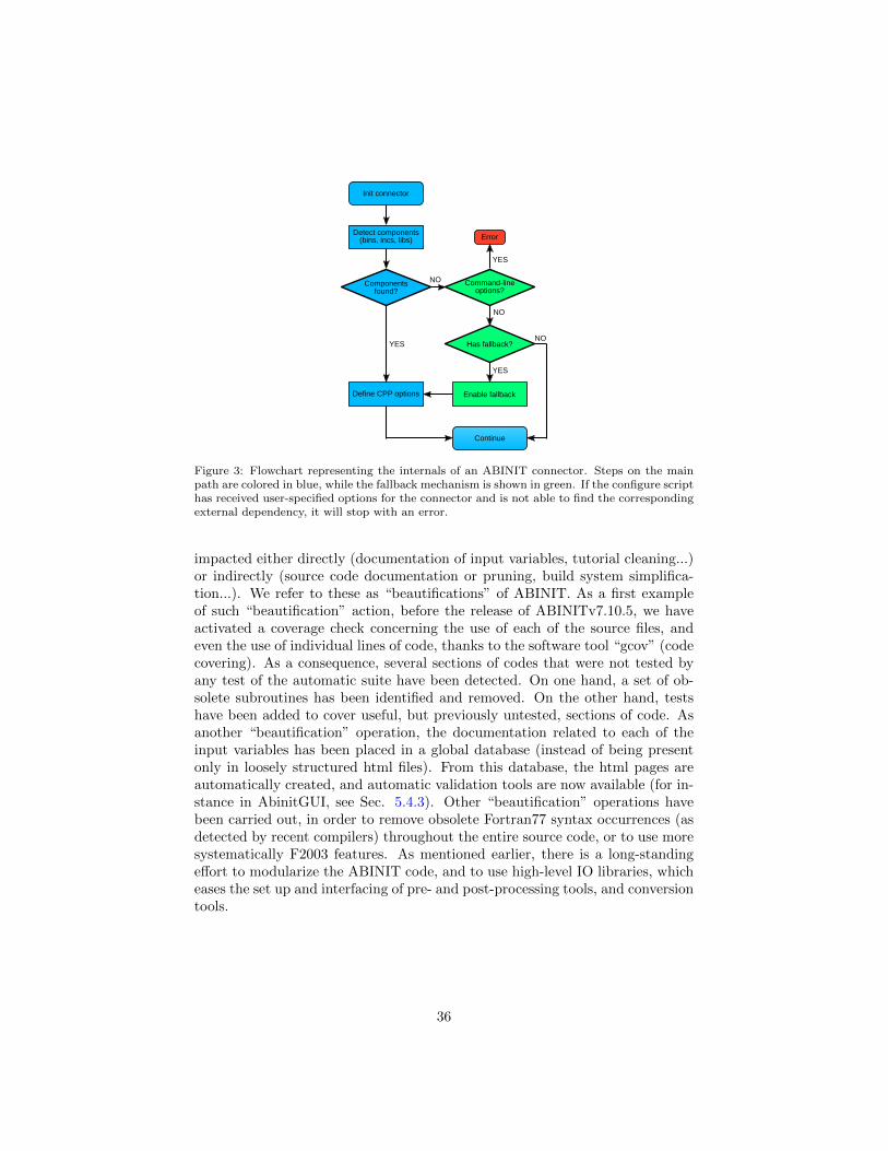
Figure 3: Flowchart representing the internals of an ABINIT connector. Steps on the mainpath are colored in blue, while the fallback mechanism is shown in green. If the configure scripthas received user-specified options for the connector and is not able to find the correspondingexternal dependency, it will stop with an error.

impacted either directly (documentation of input variables, tutorial cleaning...)or indirectly (source code documentation or pruning, build system simplifica-tion...). We refer to these as “beautifications” of ABINIT. As a first exampleof such “beautification” action, before the release of ABINITv7.10.5, we haveactivated a coverage check concerning the use of each of the source files, andeven the use of individual lines of code, thanks to the software tool “gcov” (codecovering). As a consequence, several sections of codes that were not tested byany test of the automatic suite have been detected. On one hand, a set of ob-solete subroutines has been identified and removed. On the other hand, testshave been added to cover useful, but previously untested, sections of code. Asanother “beautification” operation, the documentation related to each of theinput variables has been placed in a global database (instead of being presentonly in loosely structured html files). From this database, the html pages areautomatically created, and automatic validation tools are now available (for in-stance in AbinitGUI, see Sec. 5.4.3). Other “beautification” operations havebeen carried out, in order to remove obsolete Fortran77 syntax occurrences (asdetected by recent compilers) throughout the entire source code, or to use moresystematically F2003 features. As mentioned earlier, there is a long-standingeffort to modularize the ABINIT code, and to use high-level IO libraries, whicheases the set up and interfacing of pre- and post-processing tools, and conversiontools.

36

Spin

TDDFT

DFT+U, DMFT Determine U

PAW1, 2, 3, Proper8es at

nuclei

Source Code

Four Basic Lessons

Parallel Ground state wavelets

Parallel Response Func8ons

Parallel Many Body Perturb. Theory

Resp Func 1

Resp Func 2, elphon

elas8c, NL

Wannier90

Polariza8on

op8c

GW1

GW2, BSE

Parallel Ground state MD, Images

Intro ABINIT in parallel

Figure 4: Flowchart representing the dependencies between the tutorials of ABINIT.

5. Other developments in the ABINIT project

5.1. Documentation, tutorials and tests

The documentation of ABINIT is multifaceted. The source of most docu-mentation files can be found in doc/, and most are processed and presented onthe ABINIT Web site. One can distinguish three structured sets of informationthat guide the user : the new user guide and help files, the tutorial, and thedescription of input variables, with respective entry points on the Web

www.abinit.org/doc/helpfiles/for-v7.10/<X>,

with <X> being users/new user guide.html, tutorial/welcome.html, andinput variables/keyhr.html. In the package, they are located in doc/users,doc/tutorial, doc/input variables, respectively. The doc/ directory alsocontains the installation notes, release notes, known problems, as well as somespecific documents on the theory underlying ABINIT, information on the buildconfiguration files, and other miscellaneous information for the use of ABINITthat are not present on the Web.

While the relatively low-level user guide and help files have only seen minorchanges with respect to ABINITv5.7, the tutorial has been largely expanded,with twelve new lessons (for a total of thirty-three). Most of them are present indoc/tutorial. A flowchart representing the dependencies between the tutorialsof ABINIT is presented Fig. 4.

37

Six new lessons, mentioned in the rightmost column of Fig. 4, are related tothe use of parallel features of ABINIT(lesson paral gspw - Parallel Ground state, lesson paral moldyn - MD, lesson paral string

- Images, lesson paral gswvl - Parallel Ground state wavelets,lesson paral dfpt - Parallel Response Functions,lesson paral mbt - Parallel Many Body Perturb. Theory), and were demon-strated at a training school [123], where the participants could have access tomore than one thousand computing cores for their tests. Other lessons focus onthe BSE formalism, on dynamical mean field theory, on nuclear properties, onthe comparison between PAW and all-electron calculations, and on the deter-mination of the U value in the constrained LDA formalism (lesson bse.html,lesson dmft.html, lesson nuc.html, lesson paw3.html, lesson udet.html).At variance with all the other lessons, the new lesson on the computation of thetemperature-dependent electronic structure (including zero-point motion renor-malization) is available only on the ABINIT Wiki [124].

The other lessons are available as well on the Wiki, although, at present,their official source is in the package or on the official ABINIT Web site.

Independently of the doc/ directory, there is also a large set of exam-ple input files, with their reference output files, contained in tests/*/Input

and tests/*/Refs. These are a very useful counterpart to the input vari-able description file, as they illustrate the use of every ABINIT input vari-able, at least in one case for each input variable. Between ABINITv5.10.8 andABINITv7.10.5, the number of input files provided in tests/*/Input has in-creased from about 600 to about 1000.

Another noticeable source of documentation on ABINIT consists in the slidesthat are available on the Web, having been prepared for different schools orhands-on events. They are listed in http://www.abinit.org/community/events.As a recent side effort that aimed at investigating new ways to provide docu-mentation for ABINIT, videos for the basic steps of ABINIT usage have beenset up on YouTube, see www.youtube.com/<X> :

• How to install on Linux (<X> is watch?v=DppLQ-KQA68) ;

• How to install on Windows (<X> is watch?v=EfJcYi1MNBg) ;

• The first tutorial on H2 molecules (<X> is watch?v=gcbfb Mteo4).

5.2. The test farm

The reference input and output files play an important role in securing thecapabilities of ABINIT. Before a new development is included in the main ver-sion of ABINIT, there is a careful check that it does not destroy the existingABINIT capabilities. At the time of ABINITv5.7, this was checked thanks toscripts, but the launch and analysis on different machines was done manually.Shortly after ABINITv5.7, a test farm was set up with appropriate software,and the whole checking procedure is now completely automatic. This milestonefor the ABINIT developer community is described in detail in several sections ofRef. [125]. The test farm infrastructure has evolved since that time, but not its

38

philosophy. So, we suggest the interested reader to consult Ref. [125], insteadof rephrasing it here. By contrast, a list of the architectures and compilers, onwhich ABINIT is daily tested, might be very useful for the user and is shownin Tab. 1. Note that older compilers which do not support fortran2003 are notable to compile the latest versions of ABINIT.

At variance with the Intel, GNU, G95, NAG and IBM compilers, for whichthe test suite executes correctly (at least for some recent or not-so-recent re-lease(s) of these compilers), too many specific problems were encountered withthe PGI, Pathscale and Open64 compilers. As a consequence, they are notofficially supported, and no machine is dedicated to tests based on the executa-bles that they generate. This does not mean that ABINIT will not work withsome version of these compilers, but there is no guarantee ABINIT will compileand/or run correctly with them. Table 1 applies to production version 7.10.5,while development versions of ABINIT have also been tested successfully withthe GNU 5.1 and 5.2 compilers, as well as with the Intel 15 compilers.

In addition to the input files and corresponding reference files that testABINIT computational capabilities, the test suite also includes memory checksand profiling (yquem g95), as well as checks on the compilation (e.g., full de-bugging options for inca gcc44 sdebug and tikal gcc49), build (e.g., woopy gcc48relies on external libraries only) generation of package (shiva gcc47 distchk) andeven the coherence of the documentation of ABINIT.

5.3. Atomic data files

The Norm-Conserving pseudopotentials (NCPP) and PAW methods areboth available in ABINIT. The PAW method allows lower plane wave energycutoffs and reproduces by construction all the nodes of the valence wavefunc-tions. It is therefore particularly suited to the study of localized electrons. Thatis why the local exact exchange, the LDA+U and DMFT approaches are avail-able in ABINIT in the PAW framework only. Most of the time, new featuresare developed first in the NCPP framework, and are extended later to the PAWone because of the more complex coding required in the PAW framework. Someof the most recent features in ABINIT are therefore available only in the NCCPcase, as precised in the text hereabove.

5.3.1. Norm-Conserving pseudopotentials

At the time of ABINIT v5.8, the ABINIT project provided several NCCPtables [126, 127] on the official website, but the majority of these tables hadbeen generated without relying on optimization techniques, such as the RRKJmethod [128], and, most importantly, no systematic validation of these tableshad ever been performed. Last but not least, most of these legacy NCPPsemployed only one projector per angular channel, hence it was difficult to findNCPPs with semi-core states treated as valence. For this reason, we have gener-ated a new table of NCPPs based on the multiple-projector formalism recentlyproposed in Ref. [129]. These new pseudopotentials are usually softer than tradi-tional NCPPs and more accurate, especially when semi-core states are included

39

Builder label Compiler Parallel Numerical Other characteristicssupport libraries

testf gcc47 GNU 4.7.1 openmpi 1.6.1testf gcc47 serial GNU 4.7.1 Parallelism disabledbigmac gcc48 sl GNU 4.8.2 mpich3 3.1.1 atlas 3.10.1 Packages installed

scalapack 2.0.2 fftw3 3.3.4 with MacPortsbuda gcc47 cuda GNU 4.7.4 openmpi 1.6.5 mkl 10.3 GPU (cuda 6.5)

magma 1.5.0 K40 NVIDIA cardbuda intel14 Intel 14.0.4 mpich3 3.1.3 mkl 11.0 Compiler options

fftw3 -O3 -xhostcoba2 intel13 Intel 13.1.1 openmpi 1.6.5 mkl 11.0 CentOS

fftw3cronos gcc46 paral GNU 4.6.3 openmpi 1.4.5 mkl 10.3 Whole test suite

fftw3 executed on 2 procsibm6 xlf14 IBMxlf 14.1 poe OS : AIX6.1

inca gcc44 sdebug GNU 4.4.7 mpich3 3.1.1 atlas 3.10.1ktulu gcc48 GNU 4.8.2 openmpi 1.6.5 atlas 3.10.1 Test Ubuntu 14.0.4

fftw3 3.3.3 packagesmax2 gcc46 GNU 4.6.2 mpich2 1.4.svn acml 4.4.0 Memory profilingpetrus nag NAG 5.3.1 openmpi 1.6.5 openSUSE 12.1

shiva gcc47 distchk GNU 4.7.4 mpich2 1.3 openBLAS Make distchecktikal intel12 serial Intel 12.1.4 mkl 10.3 Parallelism disabled

fftw3tikal gcc49 GNU 4.9.2 mpich3 3.1 mkl 11.1

fftw3toum gcc46 openmp GNU 4.6.3 2 OpenMP threads

Fedoravishnu gcc47 nofbmisc GNU 4.7.4 openmpi 1.6.5

woopy gcc48 GNU 4.8.3 mpich3 3.0.4yquem g95 g95 0.94 openmpi 1.6.3 Tests with

1 proc only

Table 1: Several characteristics of the “builders” on which ABINIT v7.10.5 has been dailytested until September 2015.

40

in the valence, since the additional projector allows one to employ the neutralatomic ground state as a reference configuration, instead of an ionized atom.

This new table (ONCVPSP-PBE-PDv0.2) has been validated against all-electron calculations using the “∆” estimator proposed in Refs. [130, 131] (∆ =0.7 meV , ∆1 = 1.6 meV ) as well as the GBRV benckmark set [132]. Moreoverthe convergence behavior of phonon modes within DFPT has been tested. Asummary of the results of the validation tests is given in Figure 5. The inputfiles as well as the pseudopotential files are available on the ABINIT website, aswell as on the website [133]. The python scripts used to validate the table areavailable on the PseudoDojo repository hosted on GitHub [134].

Figure 5: Values of the ∆ factor and relative error for the lattice constants of the bcc/fccelemental solids included in the all-electron GBRV set for the ONCVPSP norm-conservingpseudopotentials. White rectangles (triangles) denote entries that are missing in the bench-mark set. The mean absolute relative error for the tests are 0.12 and 0.13 for fcc and bcc,respectively.

5.3.2. PAW atomic datasets

In the Projector Augmented Wave (PAW) method developed by Blochl(1994) [36], a PAW data file is needed for each element, which replaces thepseudopotential file used in the NCCP or USPP formalisms. We have devel-oped a new set of PAW atomic data files for most of the stable elements in theperiodic table (the JTH table [131]). They have been generated thanks to theATOMPAW generator [38]. These files are provided in a standard XML for-mat for use in any PAW electronic structure code, following the specificationsgiven in Ref. [135]. The new datasets are available on the ABINIT web site[136] for the first 86 elements. They perform well as measured by the “∆” eval-uation criterion introduced by Lejaeghere et al. [130] (periodic table average∆ = 0.4 meV ), and also perform well in a modified evaluation scheme proposedin Ref.[131] (periodic table average ∆1 = 1.3 meV ). The GBRV benckmarkset [132] gives also very good results for the JTH table, as can be seen on Fig-ure 6.

41

Figure 6: Values of the ∆ factor and relative error for the lattice constants of the bcc/fccelemental solids included in the all-electron GBRV set for the JTH PAW atomic data. Whiterectangles (triangles) denote entries that are missing in the benchmark set. The mean absoluterelative error for the tests are 0.13 and 0.14 for fcc and bcc, respectively.

5.4. Post-processing, GUIs, and scripting

5.4.1. AbiPy

The AbiPy software is a python package that provides a scripting environ-ment for the analysis and the post-processing of ABINIT calculations as wellas tools for the automatic generation of input files and the submission of jobson massively parallel architectures. AbiPy is built on top of pymatgen [137], anopen-source Python library that provides powerful tools to analyze large quan-tities of materials information [138] and a high-level interface to the MaterialsProject database [139]. The AbiPy package also contains several graphical in-terfaces that significantly simplify the repetitive work needed for extracting andvisualizing the results. Figure 7 shows a screen shot of the different capabili-ties. All the software components are hosted on GitHub [140], a social codingplatform that allows users to report bugs and contribute to development.

5.4.2. ABINIT Post Process Application (APPA)

Output files produced by large scale Molecular Dynamics (MD) simulationsare not easy to handle. Such trajectories are stored in a file named HIST (aNetCDF file) from which it may be necessary to extract data in text format.The goal of the “APPA” utility is to allow statistical analysis of MD trajectoriesthrough an ergonomic graphical user interface.

APPA is written in Python, using graphical packages such as PyQt or mat-plotlib. Some parts of this tool use Fortran — thanks to the F2PY Python pack-age, to handle large amounts of data more efficiently and to conserve numericalaccuracy in post-processing. The APPA interface is intuitive and documented(tooltips) and allows the computation of variations or averages of several prop-erties: total energy, pressure, temperature, velocity auto-correlation function,radial pair distribution, vibrational density of state, etc. APPA can manage

42

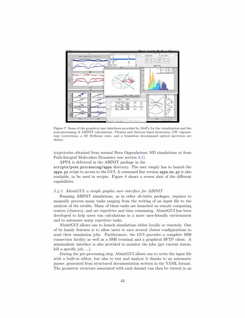
Figure 7: Some of the graphical user interfaces provided by AbiPy for the visualization and thepost-processing of ABINIT calculations. Phonon and electron band structures, GW eigenen-ergy corrections, a 3D Brillouin zone, and a transition decomposed optical spectrum areshown.

trajectories obtained from normal Born Oppenheimer MD simulations or fromPath-Integral Moleculars Dynamics (see section 3.1).

APPA is delivered in the ABINIT package in thescripts/post processing/appa directory. The user simply has to launch theappa.py script to access to the GUI. A command line version appa nw.py is alsoavailable, to be used in scripts. Figure 8 shows a screen shot of the differentcapabilities.

5.4.3. AbinitGUI: a simple graphic user interface for ABINIT

Running ABINIT simulations, as in other ab-initio packages, requires tomanually process many tasks ranging from the writing of an input file to theanalysis of the results. Many of these tasks are launched on remote computingcenters (clusters), and are repetitive and time consuming. AbinitGUI has beendeveloped to help users run calculations in a more user-friendly environmentand to automate many repetitive tasks.

AbinitGUI allows one to launch simulations either locally or remotely. Oneof its handy features is to allow users to save several cluster configurations tosend their simulation jobs. Furthermore, the GUI provides a complete SSHconnection facility as well as a SSH terminal and a graphical SFTP client. Aminimalistic interface is also provided to monitor the jobs (get current status,kill a specific job, ...).

During the pre-processing step, AbinitGUI allows one to write the input filewith a built-in editor, but also to test and analyze it thanks to an automaticparser, generated from structured documentation written in the YAML format.The geometric structure associated with each dataset can then be viewed in an

43

Figure 8: Some of the graphical user interfaces provided by APPA for the visualization andthe post-processing of ABINIT MD runs. A radial pair distribution function, velocity auto-correlation function, trajectory visualisation, and the variation of the components of the totalenergy are shown.

embedded Jmol panel [141]. As a second step, the user edits the configurationfor the specific remote job management system and launches the job. All therequired files are automatically generated and submitted to the remote system.

Finally, the user can analyze the results through a set of post-processingscripts that are shipped with the GUI. The scripts are, for instance, band struc-ture plotters, or links to the Python Library “Abipy” (see Sec 5.4.1).

This project is developed in Java to be cross-platform and therefore doesnot require any installation. As the size of the package grew with time, thedevelopers decided to extract the development from the main ABINIT packageand hosted the package on Github [142]. A dedicated website has also beendesigned, and contains the latest stable version as well as documentation andsupplementary information [143].

6. On-going developments

6.1. Unfolding supercell band structures

Supercells are often used in ab initio calculations to model compound alloys,surfaces and defects. Band structure plots obtained from supercell calculationsare difficult to interpret and compare to the reference band structure of a corre-sponding primitive crystallographic unit due to the zone folding (see the bandstructure of a Si supercell in Fig. 9a). The purpose of fold2Bloch is to assistwith interpretation of supercell electronic structure calculations by recovering

44

the Bloch character of electronic eigenstates perturbed by disorder. In gen-eral, there is no single wave-vector k associated with a particular eigenvalueE, but rather a distribution of k’s. This distribution is also known as a Blochspectral density or spectral weight. The spectral weight wn(k) amounts to aBloch k-character of the n’th energy eigenstates εn and fulfills the normalization∑

k wn(k) = 1. In the case of a non-local basis set, such as plane waves, thespectral weight can be constructed from the Fourier expansion coefficients bygathering them in groups associated with a particular Bloch wave vector in theprimitive cell [144, 145, 146, 147, 148]

wn(k) =∑G

|Cn,K(G)|2 for all G that fulfill K + G = k + g , (23)

where Cn,K(G) refers to plane wave coefficients for nth eigenstate with thewave vector K within the first Brillouin zone (BZ) of the supercell, G and gare the reciprocal lattice vectors of the supercell and primitive cell, respectively.More technical details on this unfolding procedure are available in Ref. [149]. Itshould be noted that the primitive and supercell reciprocal lattices should becommensurate as required by Eq. (23). This condition implies that a supercellneeds to be generated by translation of the primitive cell along its lattice vectorsin real space using a desired multiplicity Nx ×Ny ×Nz. Care should be takenwhen working with lattices whose conventional unit cell is different from theprimitive cell (e.g., zinc-blende or rock salt structures).

A prerequisite for unfolding is the presence of wave function files (e.g.,abo WFK) that can be generated in a way similar to standard band structurecalculations. The only difference from the conventional band structure calcula-tion is the k-path selection approach. For instance, when aiming for the bandstructure plot with Γ(0, 0, 0)− Z(0, 0, 1/2) path in the primitive Brillouin zone(BZ), the kptbounds in supercell BZ should include Z(0, 0,−1/2)−Γ(0, 0, 0)−Z(0, 0, 1/2). At first, the part Z−Γ seems redundant lying outside of the rangeof interest. However, it is easy to show that those wave vectors contribute to therange Γ−Z after unfolding. For instance, let us consider a k-point (0, 0,−K) inthe 1×1×3 supercell. This point “unfolds” into 3 k-points in the primitive BZ:(0, 0, (−K−1)/3), (0, 0,−K/3), and (0, 0, (−K+1)/3). The first two points areirrelevant for the purpose of the plot as they do not belong to the Γ−Z segment,but the last point falls into the range of interest and needs to be included.

Once the wave function file is prepared, the unfolding proceeds by invokingfold2Bloch abo WFK Nx:Ny:Nz that generates an output file abo WFK.f2b. Theoutput file contains 5 columns: the list of unfolded wave vectors (kx, ky, kz) inthe primitive BZ, the corresponding eigenvalue εn (Ha) and the Bloch spectralweight wn.

A MATLAB script ubs dots.m is designed to assist with plotting the un-folded band structure. The unfolded band structure plot is represented as ascatter plot where the size and colour of the markers carry information aboutthe Bloch character of energy bands (see the unfolded band structure of Si inFig. 9b). Users are asked to provide details about the k-path, name of the

45

L X

2.0

1.0

0.0

1.0

2.0

3.0

4.0

Wave vector

Energ

y (

eV

)

0

0.2

0.4

0.6

0.8

1

Spectr

al w

eig

ht

VBE

CBE

SiGe

Si0.7Ge0.3

Si175Ge75 VBE CBE

c

d e f

Si

b

Si

a

L X

2.0

1.0

0.0

1.0

2.0

3.0

4.0

Wave vectorE

nerg

y (

eV

)

L X

2.0

1.0

0.0

1.0

2.0

3.0

4.0

Wave vector

En

erg

y (

eV

)

EF

Figure 9: Folded (a) and effective (b, c) band structure of 250-atoms supercell unfolded tothe primitive Brillouin zone: pure Si (a, b) and random Si0.7Ge0.3 alloy (d). The Blochcharacter in Si0.7Ge0.3 alloy is well preserved at the top of the valence band (VBE), whereasthe electronic states at the bottom of the conduction band (CBE) are more disordered. Thebottom row illustrates Si175Ge75 supercell (d) and the Kohn-Sham orbitals |ψn,K(r)|2 thatcorrespond to the top of the valence band (e) and the bottom of the conduction band (f).The structure and isosurface plots were created with the help of the ABINIT cut3d utilityand VESTA 3 package [150].

fold2Bloch output file abo WFK.f2b, position of the Fermi energy, and recip-rocal lattice vectors that can be found in the main output file ab out.out.

In order to illustrate the performance of fold2Bloch, an effective band struc-ture of a Si0.7Ge0.3 (an alloy extensively used in thermoelectric applications) iscalculated (Fig. 9). The unfolded band structure of Si0.7Ge0.3 retains main fea-tures of the Si electronic structure, however not all states preserve their Blochcharacter. The valence band edge at Γ-point retains 90% of the Bloch characterthat reflects in the periodicity of Kohn-Sham orbitals. Contrary to the valenceband, the conduction band edge shows signatures of disorder, namely “amor-phous”, non-periodic electronic states with the Bloch spectral weight of lessthan 50%. This analysis allows us to conclude that the compositional disorderwill result in diminished mobility of electrons, rather than holes.

Analysis of the effective band structure of alloys can also be linked to theiroptical properties. For instance, it is possible to observe whether optical tran-sitions, which are forbidden in the host material by the crystal momentumconservation, can become allowed in the presence of perturbations due to alloyelements.

46

6.2. Interpolation technique for BSE

An accurate description of dielectric properties within the BSE formalismpresented in Sec. 3.5.1 usually requires the sampling of a large number of k-points in the Brillouin Zone. The large computational cost associated to thisdense sampling renders well-converged BSE calculations prohibitive. This isespecially true when derived properties e.g. Raman spectra are wanted [76].

Different numerical techniques have been proposed in the literature to im-prove the convergence rate. For example, Rohlfing & Louie [151] developed adouble-grid technique in which the matrix elements of the BSE Hamiltonianevaluated on a coarse grid are then interpolated towards a denser grid. Thisscheme accelerates the convergence of the dielectric function with a computa-tional cost that is significantly reduced with respect to a full calculation. Inthe spirit of this technique, we have generalized the Rohlfing & Louie approachallowing for multi-linear interpolation and we have designed efficient algorithmsbased on iterative Lanczos-Haydock algorithms. Different schemes with dif-ferent degrees of accuracy and computational load are available in ABINIT.The interested reader is referred to Ref. [152] for a more detailed description ofthe interpolation schemes including benchmarks and tests on prototype semi-conductors.

These new interpolation schemes are available in ABINITv8 with the bs interp *input variables and examples of input files are available in v67mbpt#30-#35.

6.3. Hybrid functionals

In the 2009 ABINIT article [8], the local PBE0 approximation was pre-sented: it was an application of exact exchange functional to a restricted sub-space formed by the correlated electrons of a correlated system. A more generalimplementation of hybrid functionals has been carried out in ABINIT over thelast two years. In the NCPP framework, the Fock operator has been coded. Itis now available to perform a Hartree-Fock calculation (ixc=40) or a PBE0 one(ixc=41,42). Only the total energy is available for the moment. A well con-verged LDA/GGA calculation must be performed first, to obtain good startingwavefunctions, before adding the Fock operator. Two tests are provided inv7#65 and #66. The nphf keyword allows for a local parallelisation over k-points for the calculation of the Fock operator.

In the PAW context, the Fock operator has been coded following the workof Rostgaard [153] and will be available in ABINIT version 8. The exchangeenergy is divided in 3 terms. The first one is constant and comes from theinteractions between core orbitals; the second one comes from the interactionsbetween core and valence orbitals. It is calculated thanks to pre-computed PAWdata that are provided in the PAW atomic datasets; the third one comes frominteractions between valence electrons. This last term has a component comingfrom the charge compensation density, which is calculated “on the fly”, anda component coming from on-site interactions that is already pre-calculatedin the code. The implementation is now being extended to range-separatedfunctionals.

47

6.4. Van der Waals interactions

It is well known that long range correlations responsible of van der Waalsinteractions are out of reach for both LDA and GGA approximations to theexchange-correlation energy in DFT. In recent years several methods have beendevised to include such interactions, which can be grouped into two strategies,namely ad hoc methods and self-consistent approaches. Currently ABINIT canperform calculations based on either the DFT-D methods or the vdW-WF meth-ods, as described later, both belonging to the first group.

A fully customizable implementation of the vdW-DF method [154], a self-consistent approach, and an adaptation of the strategy followed by G. Roman-Perez et al. [155] to the case of ABINIT are under development. It will offeraround 25 ajustable parameters and be delivered with graphical tools to helpusers assess the quality of their kernels. It does not only aim at performingproduction calculations with vdW-DF, but also at helping researchers who de-velop new density functionals optimised for systems requiring van-der-Waalsinteractions.

The DFT-D methods have been implemented inside ABINIT, namely DFT-D2 [156], DFT-D3 [157] and DFT-D3(BJ) [158]. In these cases, pair-wise terms(and 3-body corrections for DFT-D3 and DFT-D3(BJ)) are added to the DFTenergy, which are independent of the electronic density, in order to mimic thevdW interactions. The implementation includes the contributions of these meth-ods to forces and stresses, in view of geometry optimization, as well as to first-order response functions like dynamical matrices, clamped elastic constants andinternal strain coupling parameters.

To activate DFT-D dispersion correction, two keywords are in use: vdw xc= 5/6/7 to choose between DFT-D2, DFT-D3 and DFT-D3(BJ), and vdw tol,to control the inclusion of largely distant pairs (those giving a contributionbelow vdw tol are ignored). It is also possible to include 3-body corrections[157] (for ground-state only) with the keyword vdw tol 3bt, which also controlsthe tolerance over this term. Four tests are available for this implementation:vdwxc#10 and v7#97 to v7#99.

Methods based on maximally localized Wannier functions (MLWFs) to cal-culate vdW energy corrections have been implemented in ABINIT. In this casethe pair-wise terms come from contributions of pairs of MLWFs rather thanfrom atoms. Among the implemented methods in ABINIT it is found vdW-WF1 [159, 160] vdW-WF2 [161] and vdW-QHO-WF [162]. A full descriptionof the implementation of vdW-WF1 is reported in [163].

Selection of one of these 3 methods is achieved by using vdw xc=10/11/14respectivelly. Since vdW-WF1 and vdW-WF2 methods are approximations forthe dispersion energy of non overlapping electronic densities, it is necessary todefine the interacting fragments of the system whose dispersion energy is goingto be calculated. The latter is achieved by using the input variables vdw nfragand vdw typfrag to define the number of interacting fragments in the unit celland to assign each atom to a fragment. A given MLWF belongs to the samefragment as its closer atom. The need for defining the interacting fragments is

48

overridden in the vdW-QHO-WF, for which these input variables are not used.When dealing with periodic systems the input varible vdw supercell controlsthe number of neighbor unit cells that will be included in the calculation. Eachone of the 3 components of vdw supercell indicates the maximum number ofcells along both positive or negative directions of the corresponding primitivevector. This is useful for studying the spacial convergency of the vdW energy.It should be noticed that the user must set the variables associated to thecalculation of MLWFs and that the resulting vdW energies strongly depend onthe obtained Wannier functions. Three tests for these methods are available:wannier90#11, wannier90#12 and wannier90#13.

6.5. New G0W0 implementation

A high performance G0W0 implementation [164] has been developed withinABINIT. It is more efficient than the traditional implementation [8, 79] thanksto the treatment of the two major bottlenecks: the summations over conductionstates and the inversion of the dielectric matrix. The first bottleneck is circum-vented by converting the summations into Sternheimer equations. Note thatthe introduction of approximations beyond the G0W0 (such as analytic contin-uation [165]) is avoided thanks to use of the simplified quasiminimal residual(SQMR) algorithm [166]. Then, the second bottleneck is assessed by expressingthe dielectric matrix in a Lanczos basis, which reduces the matrix size by ordersof magnitude with respect to a plane wave basis. A model dielectric operatorhas also been developed [164] and can optionally be used to further reduce thedielectric matrix size. The resulting implementation exhibits a 500-fold speedupfor the silane molecule, without introducing approximations beyond the G0W0

formalism and the pseudopotential method. At the time of writing, the imple-mentation supports simulations of molecular systems only (only one k-point).Furthermore, it does not supports PAW and spinors. However, it supportsparallelism over bands and FFTs [39].

To compute G0W0 corrections to DFT eigenenergies, one needs to set opt-driver 66 in the input file. This type of calculation requires that the groundstate density and wavefunctions be available from disk (using getden andgetwfk). It also requires the user to specify the state to be corrected(gwls band index), the maximum allowed residual when solving the Stern-heimer equations (tolwfr), and the number of Lanczos vectors used to expressthe dielectric matrix (gwls sternheimer kmax). Note that a convergencestudy on the latter value is required to check the accuracy of the results. Sinceonly molecular systems are currently supported, the calculation also requiresthat the Coulomb potential be spherically truncated (icutcoul 0) with a radiusrcut that should be validated with a convergence study. Relevant tests can befound in v67mbpt#15 (sequential) and paral#77 (parallel).

6.6. Effective masses

The direct estimation of effective masses from DFT band curvature usingDFPT [167] has been implemented within the linear response part of ABINIT

49

[168]. This method avoids the use of finite differences to estimate these masses,which eliminates the associated numerical noise and convergence study. Tocompute the effective masses, one has to set the keyword efmas to 1 withina calculation of the derivative of ground-state wavefunctions with respect towavevector (rfelfd 1 or 2). The effective masses will then be computed for allk-points and bands present in the calculation. One can optionally specify therange of bands to be treated for each k-point with the keyword efmas nband.

An additional feature of the effective mass implementation is the correcttreatment of degenerate bands. Indeed, the concept of effective mass breaksdown at degenerate band extrema since it is no longer possible to describe bandcurvature using a tensor [169, 170]. However, using the concept of “transportequivalent effective mass” [170] and its adaptation to the k · p framework, theimplementation is able to provide the user with effective mass tensors which,while not describing the band curvature, describe accurately the contributionof the individual bands to transport properties.

The implementation supports both NCPP and PAW schemes. Spin-polarizedsystems (nspden 2) as well as spinors (nspinor 2)can be treated, although thespin-orbit interaction can only be treated in the PAW case. The treatment ofdegenerescences is limited to the extremal points of the band structure (whichare the most relevant in any case). Relevant tests can be found in v7#80 (norm-conserving pseudopotentials) and #81 (PAW).

6.7. Improvements related to dielectric susceptibilities

The Random-Phase Approximation (RPA) to the calculation of the dielec-tric function can be expressed as a sum-over-states expression when local-fieldseffects are neglected. Starting from the momentum operators matrix elementsand combining with the Kohn-Sham eigenenergies, several quantities such asfirst-order and second-order dielectric susceptibilities are then available[171, 172,173, 174].

These calculations are available in the ABINIT package via the optic plugin.First, a calculation of the ground-state wavefunctions and the derivatives withrespect to the wavevectors needs to be performed within ABINIT on a grid ofwavevectors in the Brillouin Zone. Then, the optic plugin reads these deriva-tives, the Kohn-Sham eigenenergies and calculates the dielectric susceptibilities.

In the last development version, the input file format has been changed touse fortran namelists instead of simple sequential fields. This allows for moreuser readability. Moreover, we have also implemented in the same frameworkthe expressions derived by Hughes & Sipe [172] for the calculations of Linear-Electro Optic coefficients and we have included anti-resonant contributions aswell as the scissors operator in the calculation of all second-order susceptibilities.

The description of the new input file format as well as a new version ofthe tutorial (tutorespfn#toptic 1-4) will be available in the forthcoming releaseversion. Tests for the new routines are also available in v7#114-115.

50

6.8. Meta-GGA

The development of meta-GGA in ABINIT will continue with the imple-mentation and testing of a mixing procedure for the kinetic energy density.Indeed, preliminary tests revealed persistant oscillations in the self-consistentfield cycle. Then, the forces and the stress tensor will be added accounting forthe new terms coming from the dependence of total energy on the laplacian ofthe density and on the kinetic energy density. This requires in particular thecalculation of the kinetic energy density tensor. This will allow automatic re-laxation and geometry optimization with meta-GGA functionals. Finally, oncethese on-going developments will be achieved for the norm-conserving case, thecase of PAW inplementation will be considered.

7. Summary

In this paper, we have reviewed the most recent capabilities of the ABINITcode. They are available in version v7.10.5 on the ABINIT web site. Thetests, tutorials and references mentioned here are a good starting point to beable to use these new capabilities. Some important information is also givenconcerning how to build and run ABINIT, the structure of the ABINIT package,the auxiliary files (NCPPs and PAW atomic data), and some post-processingcapabilities. We have also covered new developments, that will be available inthe forthcoming version of ABINIT : interpolation techniques for the Bethe-Salpeter equation, hybrid functionals, Van der Waals interactions, the directcomputation of effective masses.

8. Acknowledgments

This work has been supported by the FRS-FNRS (Belgium) (G.-M. R. andA.L.) through FRIA grants (S.P., M.D.G. and B.V.T.), a FNRS grant (Y.G),the PDR grant T.0238.13 (AIXPHO), and the FRFC Project No. 2.4.589.09.F. It has also been supported by the Communaute francaise de Belgique throughthe BATTAB project (ARC 14/19-057) and the TheMoTherm and AIMEDprojects (ARC 10/15-03 and 15/19-09), by the the French National ResearchAgency (ANR ”DINF-DFT” project, M.T., B.A. and C.M., grant ANR- 2010-BLANC-0425;ANR ”NEWCASTLE” project, M.T. and T.R., grant ANR- 2010-COSI-005-01) and by the CEA transversal program ”Nanoscience”, grant 4.5.3-LARGE-DMQ (M.T. and A.L.).

Several of the authors acknowledge the Curie-CCRT french supercomputingcenter of the CEA. Part of this work was performed using computational re-sources from the french HPC agency GENCI (T.R., grant x2012096871). Com-putational resources have been also provided by the supercomputing facilitiesof the Universite catholique de Louvain (CISM/UCL) and the Consortium desEquipements de Calcul Intensif en Federation Wallonie Bruxelles (CECI) fundedby the Fonds de la Recherche Scientifique de Belgique (FRS-FNRS).

51

The present research benefited from computational resources made available onthe Tier-1 supercomputer of the Federation Wallonie-Bruxelles, infrastructurefunded by the Walloon Region under the grant agreement n1117545.

F.A.A. acknowledges the UCL for an FSR complement (Fonds Special deRecherche).

Several of the authors acknowledge the National Science Foundation of China(A.Z., grant 9133202, L.H., grant 11501544, and F.L., grant 11171232), theFunds for Creative Research Groups of China under grant 11321061 (A.Z.), theNational Basic Research Program of China under grant 2011CB309703, and theNational Center for Mathematics and Interdisciplinary Sciences of the ChineseAcademy of Sciences (A.Z.), and the Program for Innovation Research in Cen-tral University of Finance and Economics (F.L.).

J.L.J., B.R., and M.C. acknowledge the Natural Sciences and EngineeringResearch Council of Canada, the Fonds de Recherche du Quebec - Nature etTechnologies, the Regroupement Quebecois sur les Materiaux de Pointe, thePhotovoltaic Innovation Network, and the FRS-FNRS (Scientific Stay grantNo. 2014/V 6/5/010-IB) for funding.

M. C., A.B. and O.R. acknowledge the support of NSERC (Natural Sciencesand Engineering Research Council of Canada).

Y.P. gratefully acknowledges financial support from the European ResearchCouncil (ERC-2010-AdG-267374), Spanish Grant FIS2013-46159-C3-1-P, Gru-pos Consolidados (IT578-13), and AFOSR Grant FA2386-15-1-0006 AOARD144088, H2020-NMP-2014 project MOSTOPHOS, GA SEP-210187476 and COSTAction MP1306 (EUSpec), as well as high-quality technical and human supportprovided by IZO-SGI SGIker of UPV/EHU and its European funding (ERDFand ESF).

C.E. acknowledges the support of Divisin de Investigacin, Creacin e Inno-vacin, UTadeo.

We thank Ph. Ghosez, R. Caracas and R. Shaltaf for their contributions tothe life of the ABINIT community and dissemination of the ABINIT package,through the organisation of workshops or tutorials.

The present addresses of the following authors are:D. Adams, nanotech@surfaces Laboratory, Empa, Swiss Federal Laboratoriesfor Materials Science and Technology, Dubendorf, Switzerland.F. Abreu Arajo, Unite Mixte de Physique, CNRS, Thales, Univ. Paris-Sud,

52

Universite Paris-Saclay, 91767, Palaiseau, FranceT. Applencourt, Laboratoire de Chimie et Physique Quantiques, UMR 5626, IR-SAMC, CNRS et Universite de Toulouse (UPS), 118 route de Narbonne, 31062Toulouse, France.C. Audouze, University of Toronto Institute for Aerospace Studies (UTIAS),4925 Dufferin Street, Toronto, Ontario M3H 5T6 Canada.A. Levitt, Universite Paris Est, CERMICS (ENPC), INRIA, F-77455 Marne-la-Vallee, France.C. Martins, Laboratoire de Chimie et Physique Quantiques, UMR 5626, IR-SAMC, CNRS et Universite de Toulouse (UPS), 118 route de Narbonne, 31062Toulouse, France.S. Ponce, Department of Materials, University of Oxford, Parks Road, OX13PH, United Kingdom.T. Rangel-Gordillo, Molecular Foundry, Lawrence Berkeley National Labora-tory, Berkeley, California 94720,USA.B. Rousseau, Via Science, Montreal, H3J 1R4, Canada.B. Xu, Physics Department and Institute for Nanoscience and Engineering, Uni-versity of Arkansas, Fayetteville, Arkansas 72701, USA.

[1] P. Hohenberg and W. Kohn. Inhomogeneous electron gas. Phys. Rev.,136(3B):B864–B871, 1964.

[2] W. Kohn and L. J. Sham. Self-consistent equations including exchangeand correlation effects. Phys. Rev., 140(4A):A1133–A1138, 1965.

[3] L. Hedin. New method for calculating the one-particle green’s functionwith application to the electron-gas problem. Phys. Rev. A, 139:796, 1965.

[4] G. Onida, L. Reining, and A. Rubio. Electronic excitations: density-functional versus many-body green’s-function approaches. Rev. Mod.Phys., 74:601–659, 2002.

[5] http://www.gnu.org/copyleft/gpl.txt.

[6] X. Gonze, J.-M. Beuken, R. Caracas, F. Detraux, M. Fuchs, G.-M. Rig-nanese, L. Sindic, M. Verstraete, G. Zerah, F. Jollet, M. Torrent, A. Roy,M. Mikami, Ph. Ghosez, J.-Y. Raty, and D.C. Allan. First-principles com-putation of material properties : the abinit software project. Comp. Mat.Science, 25:478–492, 2002.

[7] X. Gonze, M. Rignanese, M. Verstraete, J.-M. Beuken, Y. Pouillon,R. Caracas, F. Jollet, M. Torrent, G. Zerah, M. Mikami, Ph. Ghosez,M. Veithen, J.-Y. Raty, V. Olevano, F. Bruneval, L. Reining, R. Godby,G. Onida, and D.R. Hamann an D.C. Allan. A brief introduction to theabinit software package. Zeit. Kristallogr, 220:558–562, 2005.

[8] X. Gonze, B. Amadon, P.-M. Anglade, J.-M. Beuken, F. Bottin,P. Boulanger, F. Bruneval, D. Caliste, R. Caracas, M. Cote, T. Deutsch,

53

L. Genovese, Ph. Ghosez, M. Giantomassi, S. Goedecker, D.R. Hamann,P. Hermet, F. Jollet, G. Jomard, S. Leroux, M. Mancini, S. Mazevet,M.J.T. Oliveira, G. Onida, Y. Pouillon, T. Rangel, G.-M. Rignanese,D. Sangalli, R. Shaltaf, M. Torrent, M.J. Verstraete, G. Zerah, and J.W.Zwanziger. Abinit: First-principle approach to material and nanosystemproperties. Comp. Phys. Comm., 180:2582–2615, 2009.

[9] http://abinit.org.

[10] http://abinit.org/doc/helpfiles.

[11] http://forum.abinit.org.

[12] http://wiki.abinit.org/doku.php.

[13] D. Marx and M. Parrinello. Ab initio path integral molecular dynamics:Basic ideas. J. Chem. Phys., 104:4077, 1996.

[14] M. E. Tuckerman, D. Marx, M. L. Klein, and M. Parrinello. Efficient andgeneral algorithms for path integral Car–Parrinello molecular dynamics.J. Chem. Phys., 104:5579, 1996.

[15] G. Geneste, M. Torrent, F. Bottin, and P. Loubeyre. Strong isotope effectin phase II of dense solid hydrogen and deuterium. Phys. Rev. Lett.,109:155303, 2012.

[16] G. Geneste, A. Ottochian, J. Hermet, and G. Dezanneau. Proton trans-port in barium stannate: classical, semi-classical and quantum regimes.Phys. Chem. Chem. Phys., 17:19104, 2015.

[17] E. Weinan, W. Ren, and E. Vanden-Eijnden. Simplified and improvedstring method for computing the minimum energy paths in barrier-crossing events. The Journal of Chemical Physics, 126(16):164103, 2007.

[18] G. Henkelman and H. Jonsson. Improved tangent estimate in the nudgedelastic band method for finding minimum energy paths and saddle points.The Journal of chemical physics, 113(22):9978–9985, 2000.

[19] G. Mills and H. Jonsson. Quantum and thermal effects in h 2 dissocia-tive adsorption: Evaluation of free energy barriers in multidimensionalquantum systems. Phys. Rev. Lett., 72(7):1124, 1994.

[20] R. Resta. Macroscopic polarization in crystalline dielectrics: the geometricphase approach. Rev. Mod. Phys., 66:899–915, 1994.

[21] R. W. Nunes and X. Gonze. Berry-phase treatment of the homogeneouselectric field perturbation in insulators. Phys. Rev. B, 63(15):155107, 2001.

[22] I. Souza, J. Iniguez, and D. Vanderbilt. First-principles approach to insu-lators in finite electric fields. Phys. Rev. Lett., 89:117602, 2002.

54

[23] R. D. King-Smith and D. Vanderbilt. Theory of polarization of crystallinesolids. Phys. rev. B, 47(3):1651–1654, 1993.

[24] J.W. Zwanziger, J. Galbraith, Y. Kipouros, M. Torrent, M. Giantomassi,and X. Gonze. Finite homogeneous electric fields in the projector aug-mented wave formalism: Applications to linear and nonlinear response.Comput. Mater. Sci., 58:113–118, 2012.

[25] D. Vanderbilt and R. D. King-Smith. Electronic polarization in the ultra-soft pseudopotential formalism, http://arxiv.org/abs/cond-mat/9801177,1998.

[26] R. M. Nieminen, E. Boronski, and L. J. Lantto. Two-component density-functional theory: Application to positron states. Phys. Rev. B, 32:1377,1985.

[27] E. Boronski and R. M. Nieminen. Electron-positron density-functionaltheory. Phys. Rev. B, 34:3820, 1986.

[28] M. J. Puska and R. M. Nieminen. Theory of positrons in solids and onsolid surfaces. Rev. Mod. Phys., 66:841, 1994.

[29] F. Tuomisto and I. Makkonen. Defect identification in semiconductorswith positron annihilation: Experiment and theory. Rev. Mod. Phys.,85:1583, 2013.

[30] A. Kawasuso, M. Yoshikawa, H. Itoh, T. Chiba, T. Higuchi, K. Betsuyaku,F. Redmann, and R. Krause-Rehberg. Electron-positron momentum dis-tributions associated with isolated silicon vacancies in 3 C-Si C. Phys.Rev. B, 72(4):045204, 2005.

[31] P. Folegati, I. Makkonen, R. Ferragut, and M.J. Puska. Analysis ofelectron-positron momentum spectra of metallic alloys as supported byfirst-principles calculations. Phys. Rev. B, 75(5):054201, 2007.

[32] A. Calloni, A. Dupasquier, R. Ferragut, P. Folegati, M.M. Iglesias,I. Makkonen, and M.J. Puska. Positron localization effects on the dopplerbroadening of the annihilation line: Aluminum as a case study. Phys. Rev.B, 72(5):054112, 2005.

[33] C. Rauch, I. Makkonen, and F. Tuomisto. Identifying vacancy complexesin compound semiconductors with positron annihilation spectroscopy: Acase study of InN. Phys. Rev. B, 84(12):125201, 2011.

[34] J. Wiktor, X. Kerbiriou, G. Jomard, S. Esnouf, M.-F. Barthe, andM. Bertolus. Positron annihilation spectroscopy investigation of vacancyclusters in silicon carbide: Combining experiments and electronic struc-ture calculations. Phys. Rev. B, 89(15):155203, 2014.

55

[35] J. Wiktor, M.-F. Barthe, G. Jomard, M. Torrent, M. Freyss, and M. Berto-lus. Coupled experimental and DFT+ U investigation of positron lifetimesin UO2. Phys. Rev. B, 90(18):184101, 2014.

[36] P. E. Blochl. Projector augmented-wave method. Phys. Rev. B, 50:17953–17979, 1994.

[37] J. Wiktor, G. Jomard, and M. Torrent. Two-component density func-tional theory within the projector augmented-wave approach: Accurateand self-consistent computations of positron lifetimes and momentum dis-tributions. Phys. Rev. B, 92:125113, Sep 2015.

[38] N.A.W. Holzwarth, A.R. Tackett, and G.E. Matthews. A projector aug-mented wave (PAW) code for electronic structure calculations, part I:ATOMPAW for generating atom-centered functions. Comp. Phys. Comm.,135:329, 2001.

[39] F. Bottin, S. Leroux, A. Knyazev, and G. Zerah. Large-scale ab initiocalculations based on three levels of parallelization. Comp. Mat. Sci.,42(2):329–336, 2008.

[40] A. Levitt and M. Torrent. Parallel eigensolvers in plane-wave densityfunctional theory. Comp. Phys. Comm., 187:98–105, 2015.

[41] J. Wiktor, G. Jomard, M. Torrent, and M. Bertolus. Electronic structureinvestigation of energetics and positron lifetimes of fully relaxed monova-cancies with various charge states in 3C-SiC and 6H-SiC. Phys. Rev. B,87:235207, 2013.

[42] J. Wiktor, G. Jomard, and M. Bertolus. Electronic structure calculationsof positron lifetimes in SiC: Self-consistent schemes and relaxation effect.Nucl. Instrum. Meth., 327:63, 2014.

[43] A. D. Becke and K. E. Edgecombe. A simple measure of electron localiza-tion in atomic and molecular systems. J. Chem. Phys., 92(9):5397–5403,1990.

[44] A. Savin, O. Jepsen, J. Flad, O. K. Andersen, H. Preuss, and H. G. vonSchnering. Electron localization in solid-state structures of the elements:the diamond structure. Angewandte Chemie International Edition in En-glish, 31(2):187–188, 1992.

[45] R. F. W. Bader. Atoms in molecules: A quantum theory. Oxford Univer-sity Press., ISBN 978-0-19-855865-1, 1994.

[46] M. A. L. Marques, M. J. T. Oliveira, and T. Burnus. Libxc: A library ofexchange and correlation functionals for density functional theory. Com-put. Phys. Commun., 183:2272–2281, 2012.

56

[47] F. Tran and P. Blaha. Accurate band gaps of semiconductors and insu-lators with a semilocal exchange-correlation potential. Phys. Rev. Lett.,102:226401, 2009.

[48] D. Waroquiers, A. Lherbier, A. Miglio, M. Stankovski, S. Ponce, M.J.T.Oliveira, M. Giantomassi, G.-M. Rignanese, and X. Gonze. Band widthsand gaps from the Tran-Blaha functional: Comparison with many-bodyperturbation theory. Phys. Rev. B, 87:075121, 2013.

[49] E. Bousquet, N. A. Spaldin, and K. T. Delaney. Unexpectedly largeelectronic contribution to linear magnetoelectricity. Phys. Rev. Lett.,106:107202, 2011.

[50] A. Mosca Conte. Quantum mechanical modeling of nano magnetism. PhDthesis, SISSA, Trieste Italy, 2007.

[51] Pui-Wai Ma and S. L. Dudarev. Constrained density functional for non-collinear magnetism. Phys. Rev. B, 91:054420, 2015.

[52] F. Bruneval, J.-P. Crocombette, X. Gonze, B. Dorado, M. Torrent, andF. Jollet. Consistent treatment of charged systems within periodic bound-ary conditions: The projector augmented-wave and pseudopotential meth-ods revisited. Phys. Rev. B, 89:045116, 2014.

[53] P. Giannozzi, S. Baroni, N. Bonini, M. Calandra, R. Car, C. Cavaz-zoni, D. Ceresoli, G.L. Chiarotti, M. Cococcioni, I. Dabo, A. Dal Corso,S. de Gironcoli, S. Fabris, G. Fratesi, R. Gebauer, U. Gerstmann,C. Gougoussis, A. Kokalj, M. Lazzeri, L. Martin-Samos, N. Marzari,F. Mauri, R. Mazzarello, S. Paolini, A. Pasquarello, L. Paulatto, C. Sbrac-cia, S. Scandolo, G. Sclauzero, A.P. Seitsonen, A. Smogunov, P. Umari,and R.M. Wentzcovitch. QUANTUM ESPRESSO: a modular and open-source software project for quantum simulations of materials. J. Phys.:Cond. Matt., 21(39):395502, 2009.

[54] X. Gonze. First-principles responses of solids to atomic displacementsand homogeneous electric fields: Implementation of a conjugate-gradientalgorithm. Phys. Rev. B, 55:10337–10354, 1997.

[55] X. Gonze and C. Lee. Dynamical matrices, born effective charges, dielec-tric permittivity tensors, and interatomic force constants from density-functional perturbation theory. Phys. Rev. B, 55:10355, 1997.

[56] C. Audouze, F. Jollet, M. Torrent, and X. Gonze. Projector augmented-wave approach to density-functional perturbation theory. Phys. Rev. B,73:235101, 2006.

[57] C. Audouze, F. Jollet, M. Torrent, and X. Gonze. Comparison betweenprojector augmented-wave and ultrasoft pseudopotential formalisms atthe density-functional perturbation theory level. Phys. Rev. B, 78:035105,2008.

57

[58] J. M. Ziman. Electrons and phonons. Oxford University Press, 1960.

[59] P. B. Allen. New method for solving boltzmann’s equation for electronsin metals. Phys. Rev. B, 17:3725–3734, 1978.

[60] P. B. Allen. Boltzmann theory and resistivity of metals. In J. R. Che-likowsky and S. G. Louie, editors, Quantum Theory of Real Materials,pages 219–250. Kluwer, Boston, 1996.

[61] G. Grimvall. The electron phonon interaction in metals. North-Holland,Amsterdam, 1981.

[62] S.Y. Savrasov and D.Y. Savrasov. Electron-phonon interactions and re-lated physical properties of metals from linear-response theory. Phys. Rev.B, 54:16487, 1996.

[63] B. Xu and M. J. Verstraete. First principles explanation of the positiveseebeck coefficient of Lithium. Phys. Rev. Lett., 112:196603, 2014.

[64] O. D. Restrepo, K. Varga, and S. T. Pantelides. First-principles calcu-lations of electron mobilities in silicon: Phonon and coulomb scattering.App. Phys. Lett., 94(21), 2009.

[65] P. B. Allen and V Heine. Theory of the temperature dependence of elec-tronic band structures. J. of Phys. C: Solid State Physics, 9:2305, 1976.

[66] P. B. Allen and M. Cardona. Theory of the temperature dependence ofthe direct gap of germanium. Phys. Rev. B, 23:1495–1505, 1981.

[67] P. B. Allen and M. Cardona. Temperature dependence of the direct gapof Si and Ge. Phys. Rev. B, 27:4760–4769, 1983.

[68] S. Baroni, P. Giannozzi, and A. Testa. Green’s-function approach to linearresponse in solids. Phys. Rev. Lett., 58:1861–1864, 1987.

[69] S. Ponce, G. Antonius, Y. Gillet, P. Boulanger, J. Laflamme Janssen,A. Marini, M. Cote, and X. Gonze. Temperature dependence of electroniceigenenergies in the adiabatic harmonic approximation. Phys. Rev. B,90:214304, 2014.

[70] S. Ponce, G. Antonius, P. Boulanger, E. Cannuccia, A. Marini, M. Cote,and X. Gonze. Verification of first-principles codes: Comparison of to-tal energies, phonon frequencies, electronphonon coupling and zero-pointmotion correction to the gap between ABINIT and QE/Yambo. Comp.Mat. Sci., 83:341 – 348, 2014.

[71] X. Gonze, P. Boulanger, and M. Cote. Theoretical approaches to the tem-perature and zero-point motion effects on the electronic band structure.Annalen der Physik, 523:168, 2011.

58

[72] S. Ponce, Y. Gillet, J. Laflamme Janssen, A. Marini, M. Verstraete, andX. Gonze. Temperature dependence of the electronic structure of semi-conductors and insulators. J. Chem. Phys., 143:102813, 2015.

[73] https://wiki.abinit.org/doku.php?id=howto:temperature.

[74] G. Antonius, S. Ponce, P. Boulanger, M. Cote, and X. Gonze. Many-bodyeffects on the zero-point renormalization of the band structure. Phys. Rev.Lett., 112:215501, 2014.

[75] G. Antonius, S. Ponce, E. Lantagne-Hurtubise, G. Auclair, X. Gonze,and M. Cote. Dynamical and anharmonic effects on the electron-phononcoupling and the zero-point renormalization of the electronic structure.Phys. Rev. B, 92:085137, 2015.

[76] Y. Gillet, M. Giantomassi, and X. Gonze. First-principles study of exci-tonic effects in raman intensities. Phys. Rev. B, 88:094305, 2013.

[77] L. He, F. Liu, G. Hautier, M. J. T. Oliveira, M. A. L. Marques, F. D. Vila,J. J. Rehr, G.-M. Rignanese, and A. Zhou. Accuracy of generalized gradi-ent approximation functionals for density-functional perturbation theorycalculations. Phys. Rev. B, 89:064305, 2014.

[78] S. Albrecht, L. Reining, R. Del Sole, and G. Onida. Ab initio calculationof excitonic effects in the optical spectra of semiconductors. Phys. Rev.Lett., 80:4510–4513, 1998.

[79] M. Giantomassi, M. Stankovski, R. Shaltaf, M. Gruning, F. Bruneval,P. Rinke, and G.M. Rignanese. Electronic properties of interfaces anddefects from many-body perturbation theory: Recent developments andapplications. Physica Status Solidi B, 248(2):275–289, 2011.

[80] G. Cappellini, R. Del Sole, L. Reining, and F. Bechstedt. Model dielectricfunction for semiconductors. Phys. Rev. B, 47:9892–9895, Apr 1993.

[81] R. Haydock. The recursive solution of the Schrodinger equation. Comp.Phys. Comm., 20(1):11 – 16, 1980.

[82] L. X. Benedict, E. L. Shirley, and R. B. Bohn. Optical absorption ofinsulators and the electron-hole interaction: An Ab Initio calculation.Phys. Rev. Lett., 80:4514–4517, 1998.

[83] M. C. Payne, M. P. Teter, D. C. Allan, T. A. Arias, and J. D. Joannopou-los. Iterative minimization techniques for ab initio total-energy calcu-lations: molecular dynamics and conjugate gradients. Rev. Mod. Phys.,64:1045–1097, 1992.

[84] J. Lindhard. On the properties of a gas of charged particles. Mat. Fys.Medd. Dan. Vid. Selsk., 28:8, 1954.

59

[85] I. Campillo, J. M. Pitarke, and A. G. Eguiluz. Electronic stopping powerof aluminum crystal. Phys. Rev. B, 58:10307 – 10314, 1998.

[86] S. Lebegue, J. Harl, T. Gould, J. G. Angyan, G. Kresse, and J. F.Dobson. Cohesive properties and asymptotics of the dispersion interac-tion in graphite by the random phase approximation. Phys. Rev. Lett.,105:196401, 2010.

[87] F. Bruneval. Range-separated approach to the RPA correlation appliedto the van der waals bond and to diffusion of defects. Phys. Rev. Lett.,108:256403, 2012.

[88] F. Bruneval and X. Gonze. Accurate GW self-energies in a plane-wavebasis using only a few empty states: Towards large systems. Phys. Rev.B, 78:085125.

[89] J. Harl, L. Schimka, and G. Kresse. Assessing the quality of the ran-dom phase approximation for lattice constants and atomization energiesof solids. Phys. Rev. B, 81:115126, 2010.

[90] F. Aryasetiawan, M. Imada, A. Georges, G. Kotliar, S. Biermann, andA. I. Lichtenstein. Frequency-dependent local interactions and low-energyeffective models from electronic structure calculations. Phys. Rev. B,70(19):195104–, 2004.

[91] B. Amadon, T. Applencourt, and F. Bruneval. Screened coulomb inter-action calculations: cRPA implementation and applications to dynamicalscreening and self-consistency in uranium dioxide and cerium. Phys. Rev.B, 89:125110, 2014.

[92] B.-C. Shih, Y. Zhang, W. Zhang, and P. Zhang. Screened coulomb inter-action of localized electrons in solids from first principles. Phys. Rev. B,85(4):045132, 2012.

[93] R. Sakuma and F. Aryasetiawan. First-principles calculations of dynami-cal screened interactions for the transition metal oxides MO (M=Mn, Fe,Co, Ni). Phys. Rev. B, 87(16):165118, 2013.

[94] B Amadon. A self-consistent DFT+DMFT scheme in the projector aug-mented wave method: applications to cerium, Ce2O3 and Pu2O3 with theHubbard I solver and comparison to DFT+U. J. Phys.: Cond. Matt.,24(7):075604, 2012.

[95] M. Cococcioni and S. de Gironcoli. Linear response approach to the cal-culation of the effective interaction parameters in the LDA+U method.Phys. Rev. B, 71(3):035105, 2005.

[96] V. I. Anisimov and O. Gunnarsson. Density-functional calculation of ef-fective coulomb interactions in metals. Phys. Rev. B, 43(10):7570–7574,1991.

60

[97] A. I. Liechtenstein, V. I. Anisimov, and J. Zaanen. Density-functional the-ory and strong interactions: Orbital ordering in mott-hubbard insulators.Phys. Rev. B, 52(8):R5467–R5470, 1995.

[98] γ and β cerium: LDA+U calculations of ground-state parameters.

[99] A. Georges, G. Kotliar, W. Krauth, and M.J. Rozenberg. Dynamicalmean-field theory of strongly correlated fermion systems and the limit ofinfinite dimensions. Rev. Mod. Phys., 68:13–125, 1996.

[100] A. Georges. Strongly correlated electron materials: Dynamical mean-fieldtheory and electronic structure. AIP Conf. Proc., 715(1):3–74, 2004.

[101] G. Kotliar, S. Y. Savrasov, K. Haule, V. S. Oudovenko, O. Parcollet,and C. A. Marianetti. Electronic structure calculations with dynamicalmean-field theory. Rev. Mod. Phys., 78(3):865–951, 2006.

[102] B. Amadon, F. Lechermann, A. Georges, F. Jollet, T. O. Wehling, andA. I. Lichtenstein. Plane-wave based electronic structure calculations forcorrelated materials using dynamical mean-field theory and projected localorbitals. Phys. Rev. B, 77(20):205112, 2008.

[103] E. Gull, A.J. Millis, A. I. Lichtenstein, A.N. Rubtsov, M. Troyer, andP. Werner. Continuous-time monte carlo methods for quantum impuritymodels. Rev. Mod. Phys., 83(2):349–404, 2011.

[104] J. Bieder and B. Amadon. Thermodynamics of the α − γ transition incerium from first principles. Phys. Rev. B, 89:195132, 2014.

[105] D. Bergeron and A.-M. S. Tremblay. Algorithms for optimized maximumentropy and diagnostic tools for analytic continuation. ArXiv e-prints,July 2015.

[106] B. Amadon, S. Biermann, A. Georges, and F. Aryasetiawan. The α − γTransition of Cerium Is Entropy Driven. Phys. Rev. Lett., 96:066402,2006.

[107] P. Werner, A. Comanac, L. de Medici, M. Troyer, and A.J. Millis.Continuous-time solver for quantum impurity models. Phys. Rev. Lett.,97(7):076405, 2006.

[108] I. Daubechies. 10 Lectures on Wavelets. Society for Industrial and Ap-plied Mathematics (SIAM, 3600 Market Street, Floor 6, Philadelphia, PA19104), 1992.

[109] S. Goedecker, M. Teter, and J. Hutter. Separable dual-space gaussianpseudopotentials. Phys. Rev. B, 54(3):1703–1710, 1996.

[110] C. Hartwigsen, S. Goedecker, and J. Hutter. Relativistic separable dual-space Gaussian pseudopotentials from h to rn. Phys. Rev. B, 58(7):3641–3662, 1998.

61

[111] L. Genovese, L. Neelov, S. Goedecker, T. Deutsch, S. Alireza Ghasemi,A. Willand, D. Caliste, O. Zilberberg, M. Rayson, A. Bergman, andR. Schneider. Daubechies wavelets as a basis set for density functionalpseudopotential calculations. J. Chem. Phys., 129:014109, 2008.

[112] T. Rangel, D. Caliste, L. Genovese, and M. Torrent. A wavelet-based pro-jector augmented-wave (PAW) method: the PAW library. to be published,2015.

[113] http://hpcforge.org/plugins/mediawiki/wiki/abinit/index.php.

[114] http://icl.cs.utk.edu/magma.

[115] http://icl.cs.utk.edu/plasma.

[116] A. Marek, V. Blum, R. Johanni, V. Havu, B. Lang, T. Auckenthaler,A. Heinecke, H.-J. Bungartz, and H. Lederer. The ELPA library: scalableparallel eigenvalue solutions for electronic structure theory and computa-tional science. J. Phys.: Cond. Matt., 26(21):1–15, 2014.

[117] A. Harju, T. Siro, F. Federici Canova, S. Hakala, and T. Rantalaiho.Computational physics on graphics processing units. Lecture Notes inComputer Science, 7782:3–26, 2013.

[118] S. Maintz, B. Eck, and R. Dronskowski. Speeding up plane-waveelectronic-structure calculations using graphics-processing units. Comp.Phys. Comm., 182(7):1421–1427, 2012.

[119] L. Genovese, M. Ospici, T. Deutsch, J.-F. Mehaut, A. Neelov, andS. Goedecker. Density functional theory calculation on many-cores hy-brid CPU-GPU architectures in hybrid architecture. J. Chem. Phys.,131:034103, 2009.

[120] H. Rutishauser. Simultaneous iteration method for symmetric matrices.Numerische Mathematik, 16(3):205–223, 1970.

[121] Y. Zhou, Y. Saad, M.L Tiago, and J. R. Chelikowsky. Self-consistent-fieldcalculations using chebyshev-filtered subspace iteration. J. Comp. Phys.,219(1):172–184, 2006.

[122] Y. Zhou, Y. Saad, M.L. Tiago, and J.R. Chelikowsky. Parallel self-consistent-field calculations via chebyshev-filtered subspace acceleration.Phys. Rev. E, 74:066704, 2006.

[123] http://sites.google.com/site/abinit2011tutorial.

[124] http://wiki.abinit.org/doku.php?id=howto:temperature.

[125] Y. Pouillon, J. M. Beuken, T. Deutsch, M. Torrent, and X. Gonze. Orga-nizing software growth and distributed development: the case of ABINIT.Comput. Sci. Eng., 13:62.

62

[126] D.R. Hamann, M. Schluter, and C. Chiang. Norm-conserving pseudopo-tentials. Phys. Rev. Lett., 43:1494–1497, 1979.

[127] G.B. Bachelet, D.R. Hamann, and M. Schluter. Pseudopotentials thatwork: From H to Pu. Phys. Rev. B, 26:4199–4228, 1982.

[128] A.M. Rappe, K.M. Rabe, E.s Kaxiras, and J.D. Joannopoulos. Optimizedpseudopotentials. Phys. Rev. B, 41:1227–1230, 1990.

[129] D. R. Hamann. Optimized norm-conserving vanderbilt pseudopotentials.Phys. Rev. B, 88:085117, 2013.

[130] K. Lejaeghere, V. Van Speybroeck, G. Van Oost, and S. Cottenier. Er-ror estimates for solid-state density-functional theory predictions: anoverview by means of the ground-state elemental crystals. Crit. Rev. SolidState Mater. Sci., 39:1, 2014.

[131] F. Jollet, M. Torrent, and N. Holzwarth. Generation of projectoraugmented-wave atomic data: a 71 element validated table in the XMLformat. Comp. Phys. Comm., 185:1246–1254, 2014.

[132] K.F. Garrity, J.W. Bennett, K.M. Rabe, and D. Vanderbilt. Pseudopo-tentials for high-throughput DFT calculations. Comp. Mat. Sci., 81:446– 452, 2014.

[133] http://www.pseudo dojo.org.

[134] http://gitlab.abinit.org/pseudo dojo.

[135] http://esl.cecam.org/mediawiki/index.php/Paw xml.

[136] http://abinit.org/downloads/PAW2.

[137] http://github.com/materialsproject/pymatgen.

[138] S.P. Ong, W.D. Richards, A. Jain, Hautier. G., M. Kocher, S. Cholia,D. Gunter, V.L. Chevrier, K.A. Persson, and G. Ceder. Python materialsgenomics (pymatgen): A robust, open-source python library for materialsanalysis. Comp. Mat. Sci., 68(0):314 – 319, 2013.

[139] http://www.materialsproject.org.

[140] http://gitlab.abinit.org/abipy.

[141] Jmol: an open-source Java viewer for chemical structures in 3D. http://www.jmol.org/.

[142] http://github.org/abinitgui/abinitgui.

[143] http://gui.abinit.org.

63

[144] L.-W. Wang, L. Bellaiche, S.-H. Wei, and A. Zunger. Majority represen-tation of alloy electronic states. Phys. Rev. Lett., 80:4725, 1998.

[145] V. Popescu and A. Zunger. Effective band structure of random alloys.Phys. Rev. Lett., 104:236403, 2010.

[146] V. Popescu and A. Zunger. Extracting e versus k effective band struc-ture from supercell calculations on alloys and impurities. Phys. Rev. B,85:085201, 2012.

[147] P. B. Allen, T. Berlijn, D. A. Casavant, and J. M. Soler. Recoveringhidden bloch character: Unfolding electrons, phonons, and slabs. Phys.Rev. B, 87:085322, 2013.

[148] Paulo V. C. Medeiros, Sven Stafstrom, and Jonas Bjork. Effects of ex-trinsic and intrinsic perturbations on the electronic structure of graphene:Retaining an effective primitive cell band structure by band unfolding.Phys. Rev. B, 89:041407, 2014.

[149] O. Rubel, A. Bokhanchuk, S. J. Ahmed, and E. Assmann. Unfolding theband structure of disordered solids: from bound states to high-mobilitykane fermions. Phys. Rev. B, 90:115202, 2014.

[150] K. Momma and F. Izumi. Vesta3 for three-dimensional visualizationof crystal, volumetric and morphology data. J. Appl. Crystallogr.,44(6):1272–1276, 2011.

[151] M. Rohlfing and S.G. Louie. Electron-hole excitations and optical spectrafrom first principles. Phys. Rev. B, 62:4927–4944, 2000.

[152] Y. Gillet, M. Giantomassi, and X. Gonze. Efficient interpolation techniquefor bethe-salpeter calculation of optical spectra. Comput. Phys. Comm.,2016. In press.

[153] C. Rostgaard. Exact exchange in density functional calculations. M.S.Thesis, Technical University of Denmark, 2006.

[154] M. Dion, H. Rydberg, E. Schroder, D. C. Langreth, and B. I. Lundqvist.Van der waals density functional for general geometries. Phys. Rev. Lett.,92:246401, 2004. Erratum: DOI:10.1103/PhysRevLett.95.109902.

[155] G. Roman-Perez and J.M. Soler. Efficient implementation of a Van derWaals density functional: Application to double-wall carbon nanotubes.Phys. Rev. Lett., 103:096102, 2009.

[156] S. Grimme. Semiempirical GGA-type density functional constructed witha long-range dispersion correction. J. Comput. Chem., 27:1787, 2006.

[157] S. Grimme, J. Anthony, S. Ehrlich, and H. Krieg. A consistent and accu-rate ab initio parametrization of density functional dispersion correction(DFT-D) for the 94 elements H-Pu. J. Chem. Phys., 132:154104, 2010.

64

[158] S. Grimme, S. Ehrlich, and L. Goerigk. Effect of the damping func-tion in dispersion corrected density functional theory. J. Comput. Chem.,32:1456–1465, 2011.

[159] P. L. Silvestrelli. van der Waals interactions in DFT made easy by Wannierfunctions. Phys. Rev. Lett., 100:053002, 2008.

[160] P. L. Silvestrelli. van der Waals interactions in density functional theoryusing Wannier functions. J. Phys. Chem. A, 113:5224, 2009.

[161] A. Ambrosetti and P. L. Silvestrelli. van der Waals interactions in densityfunctional theory using wannier functions: Improved C6 and C3 coeffi-cients by a different approach. Phys. Rev. B, 85:073101, 2012.

[162] P. L. Silvestrelli. van der Waals interactions in density functional theory bycombining the quantum harmonic oscillator-model with localized Wannierfunctions. J. Chem. Phys., 139:054106, 2013.

[163] C. Espejo, T. Rangel, Y. Pouillon, A. H. Romero, and X. Gonze. Wannierfunctions approach to van der Waals interactions in ABINIT. Comp. Phys.Comm., 183:480, 2012.

[164] J. Laflamme Janssen, B. Rousseau, and M. Cote. Efficient dielectric ma-trix calculations using the Lanczos algorithm for fast many-body G0W0

implementations. Phys. Rev. B, 91(12):125120, 2015.

[165] M. Rieger, L. Steinbeck, I. D. White, H. N. Rojas, and R. W. Godby. TheGW space-time method for the self-energy of large systems. Comp. Phys.Comm., 117(3):211–228, 1999.

[166] R. W. Freund and N. M. Nachtigal. Software for simplified Lanczos andQMR algorithms. Applied Numerical Mathematics, 19:319, 1995.

[167] X. Gonze. Adiabatic density-functional perturbation theory. Phys. Rev.A, 52(2):1096–1114, 1995.

[168] J. Laflamme Janssen, Y. Gillet, S. Ponce, A. Martin, M. Torrent, andX. Gonze. Accurate effective masses from density functional perturbationtheory. in preparation.

[169] J.M. Luttinger and W. Kohn. Motion of Electrons and Holes in PerturbedPeriodic Fields. Phys. Rev., 97(4):869–883, 1955.

[170] N.A. Mecholsky, L. Resca, I.L. Pegg, and M. Fornari. Theory of bandwarping and its effects on thermoelectronic transport properties. Phys.Rev. B, 89(15):155131, 2014.

[171] J. E. Sipe and E. Ghahramani. Nonlinear optical response of semiconduc-tors in the independent-particle approximation. Phys. Rev. B, 48:11705–11722, 1993.

65

[172] J. L. P. Hughes and J. E. Sipe. Calculation of second-order optical re-sponse in semiconductors. Phys. Rev. B, 53:10751–10763, 1996.

[173] S. Sharma, J. K. Dewhurst, and C. Ambrosch-Draxl. Linear and second-order optical response of III-V monolayer superlattices. Phys. Rev. B,67:165332, 2003.

[174] S. Sharma and C. Ambrosch-Draxl. Second-Harmonic optical responsefrom first principles. Phys. Scripta, 2004:128, 2004.

66