Recursive Structures and Processes

Curran Kelleher

July 7, 2007

Chapter 1

Recursive Structures andProcesses

“Every computer program is a model, hatched in the mind, of a real or men-tal process. These processes, arising from human experience and thought,are huge in number, intricate in detail, and at any time only partially un-derstood. They are modeled to our permanent satisfaction rarely by our com-puter programs. Thus even though our programs are carefully handcrafteddiscrete collections of symbols, mosaics of interlocking functions, they con-tinually evolve: we change them as our perception of the model deepens,enlarges, generalizes until the model ultimately attains a metastable placewithin still another model with which we struggle.” - Alan J. Perlis

1.1 Computer Programming

The above quote is from the forward to the book Structure and Interpre-tation of Computer Programs (SICP) by Harold Abelson and Gerald JaySussman. This book has become a highly revered text in the field of com-puter science. Alan Perlis sums up quite nicely the nature of the beast:computer programming is amazing, but we can never achieve the perfectionthat we instinctively seek.

As Perlis says, computer programs are “mosaics of interlocking func-tions.” When a function calls itself, it is called recursive. The nature ofprogramming is itself recursive. Programming languages are defined bygrammars which are recursive, which is why programming has infinite possi-bilities. On a higher level, the programmer is always seeking to abstract andgeneralize essential pieces, so that they can be re-used in different contexts

1

instead of re-written. The programmer tries to repeat this process on thenew code (recursion), always attempting to find the most elegant solutionto the problem at hand. Eventually the program arrives at a “metastableplace within still another model with which we struggle.” If and when inthe future that model itself is transcended, the new model will be inside yeta higher meta-model (recursion), and so on. The higher up this pyramid ofmodels, the more perfect the program seems. However, this pyramid has noend. This is why perfection is impossible.

1.2 Examples

We will learn about recursion by example, using the Groovy programminglanguage (yes, it really is Groovy). These examples are intended to beinvestigated by interested people, and often in their construction efficiencyhas been sacrificed for clarity. You will get a sense of how they work, but youwill probably not fully grok them unless you rewrite them yourself. (grok: tounderstand something so well that it is fully absorbed into oneself) Nothingis fully grokked unless you do it yourself, so I encourage you to re-implementthese examples. Make them better, faster, interactive, more interesting,more general, more beautiful, and share your discoveries with the world.

Computer programming is complex, no doubt, and if you are unfamiliarwith programming you may initially feel overwhelmed by these examples.The purpose of these examples is to teach you about recursion, so the mostimportant thing to keep in mind is not the details of each example, butrather the common theme of all of them - recursion.

1.2.1 Factorial!

We will begin with the example of the factorial, denoted “!”.

3! = 3 ∗ 2 ∗ 1 (1.1)5! = 5 ∗ 4 ∗ 3 ∗ 2 ∗ 1 (1.2)

X! = X ∗ (X − 1) ∗ (X − 2) ∗ (X − 3) ∗ ... ∗ 3 ∗ 2 ∗ 1 (1.3)0! = 1 (1.4)

So how can we compute this!? Here is a recursive function that does it:

2

First a bit of code explaination. The keyword def means define. In thiscase, we are using it to define a function. def is also used to define variables.The (n) means that the function takes a single argument, and inside thefunction it will be referred to as n. The statement for(i in 1..n) meansto do something n times, giving the variable i the current value (0, 1, 2,3, ... n-1, n). The keyword return returns a value from the function. Thestatement factorial(i) calls the function factorial, passing whateveris in the variable i as the argument (which is referred to as n inside thefunction). Surrounding text with "" makes it a string literal. The + oper-ator, when applied to strings, concatenates them together (adds the secondstring to the end of the first one). The function println prints a string tothe console.

Lets look at the algorithm. It evaluates the recursive definition of !, whichis n! = (n− 1)! for n > 1, and n! = 1 for n ≤ 1. If the function were definedonly as return n * factorial(n-1), then the function would call itselfinfinitely and never return. It must “bottom out” in order to do anything.This is true for all recursive functions. In this case, the function bottomsout when n is n ≤ 1 1 - it returns 1.

When this program is executed, we get the following output.factorial(2) = 2factorial(3) = 6factorial(4) = 24factorial(5) = 120factorial(6) = 720factorial(7) = 5040factorial(8) = 40320factorial(9) = 362880factorial(10) = 3628800

1.2.2 Fibonacci Numbers

The Fibonacci sequence can be generated by a recursive function very similarto the recursive factorial function. The only difference is the rule, which

3

for the Fibonacci sequence is f(n) = f(n − 1) + f(n − 2) for n > 1, andf(n) = 1 for n ≤ 1. This kind of recursive definition appears frequently inmathematics, and is also called a recurrence relation.

The output of this program is the Fibonacci sequence:

fibonacci(0) = 1fibonacci(1) = 1fibonacci(2) = 2fibonacci(3) = 3fibonacci(4) = 5fibonacci(5) = 8fibonacci(6) = 13fibonacci(7) = 21fibonacci(8) = 34fibonacci(9) = 55fibonacci(10) = 89

Do you find is curious that two things that on the surface seem vastlydifferent are in fact almost the same?

1.2.3 Recursive Transition Networks

On page 132 of Godel, Escher, Bach, you will find diagrams representingtwo recursive transition networks (RTNs), which define a grammar. Whenthis grammar is iterated through randomly, it can generate sentences. Hereis a program which carries out those RTNs, choosing transitions randomlywhenever there are several options.

4

Here is some sample output:

small small bagel inside the strange cowa small cow that small great cow gobbledthe horncowlarge small bagel that runs small large hornsmall hornstrange bagel with horn

1.2.4 A Tree Fractal

Now we’ll begin to generate pictures using recursion.This how fractals are generated. This program growsa tree recursively, by adding two branches to the endof the current branch until it bottoms out. Bot-toming out happens when the tree has branched acertain number of times. The size of the two newbranches relative to the current one is determined bythe sizeFactor variable. The angle at which the twonew branches will branch out relative to the currentone is determined by the angleFactor variable. The height of the first tree

5

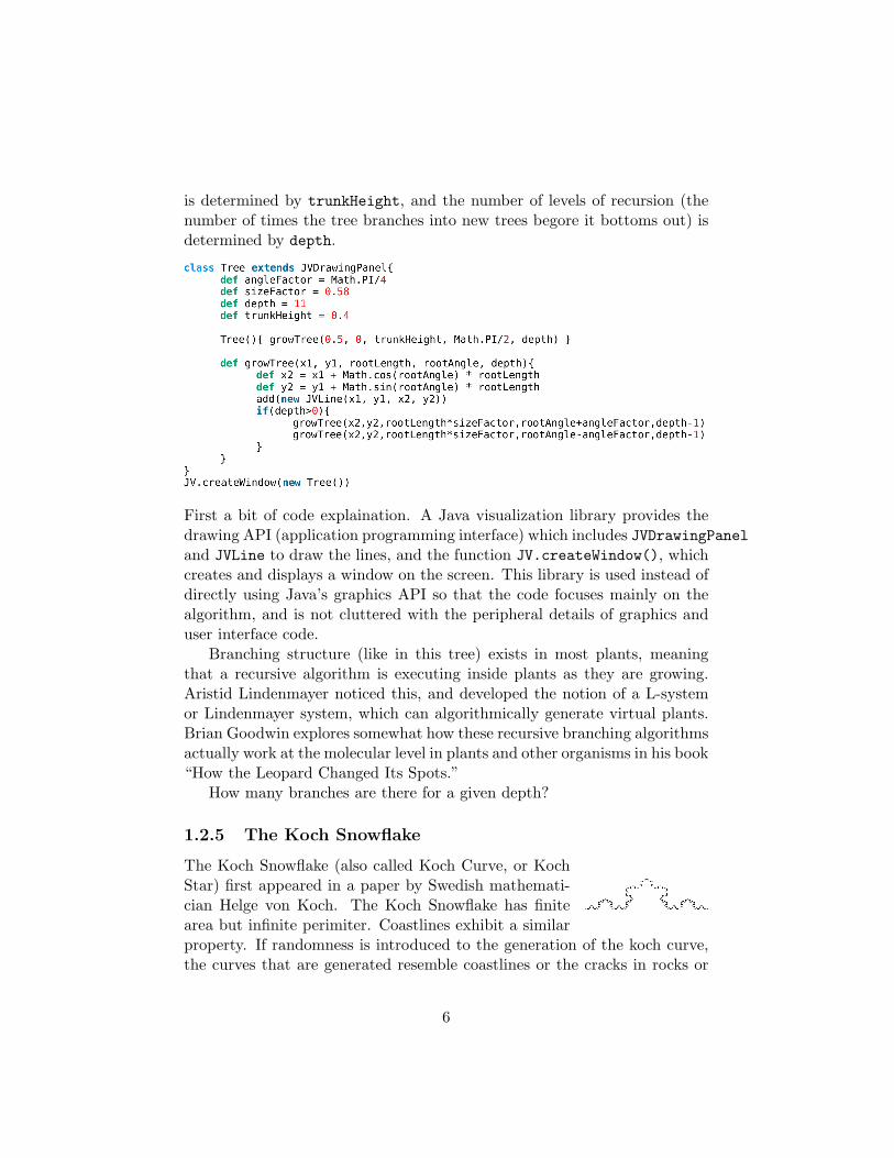
is determined by trunkHeight, and the number of levels of recursion (thenumber of times the tree branches into new trees begore it bottoms out) isdetermined by depth.

First a bit of code explaination. A Java visualization library provides thedrawing API (application programming interface) which includes JVDrawingPaneland JVLine to draw the lines, and the function JV.createWindow(), whichcreates and displays a window on the screen. This library is used instead ofdirectly using Java’s graphics API so that the code focuses mainly on thealgorithm, and is not cluttered with the peripheral details of graphics anduser interface code.

Branching structure (like in this tree) exists in most plants, meaningthat a recursive algorithm is executing inside plants as they are growing.Aristid Lindenmayer noticed this, and developed the notion of a L-systemor Lindenmayer system, which can algorithmically generate virtual plants.Brian Goodwin explores somewhat how these recursive branching algorithmsactually work at the molecular level in plants and other organisms in his book“How the Leopard Changed Its Spots.”

How many branches are there for a given depth?

1.2.5 The Koch Snowflake

The Koch Snowflake (also called Koch Curve, or KochStar) first appeared in a paper by Swedish mathemati-cian Helge von Koch. The Koch Snowflake has finitearea but infinite perimiter. Coastlines exhibit a similarproperty. If randomness is introduced to the generation of the koch curve,the curves that are generated resemble coastlines or the cracks in rocks or

6

pavement. When this randomized Koch curve is generalized into 3 dimen-sions, fractal surfaces are formed that resemble real mountains.

1.2.6 Iterated Function Systems

Iterated Function Systems (IFS) take a single point and move it around re-peatedly, plotting a point on the screen for each move. The point is movedaccording to a mapping function, which is chosen probabalistically fromseveral possible mapping functions. The Sierpinski Triangle and Fern arenotable IFS examples. Electric Sheep, the famous evolving fractal screensaver developed by Scott Draves, uses an IFS with non-linear mapping func-tions (with some other fancy tricks) to generate it’s beautiful images.

The Sierpinski Triangle

The Sierpinski Triangle (or Sierpinski Gasket) was described by Wac lawSierpinski in 1915. The Sierpinski Triangle can be obtained a number of

7

different ways. Pascal’s Triangle, when the odd numbers are colored, ap-proaches the Sierpinski Triangle as it is expanded infinitely.

Fern

The fern IFS is a system of four mapping functions. Each of these functionsis a mapping from the outermost rectangle to another, smaller rectangle.

8

Figure 1.1: The rectangles used in the coordinate transformations (approx-imately), and the image generated by our program.

The four mapping functions map from any point inside the outermost blackrectangle

1. to a point on the green part of the stem (1% of the time)

2. to a point in the red rectangle, the lowest left branch (7% of the time)

3. to a point in the dark blue rectangle, the lowest right branch (7% ofthe time)

4. to a point in the light blue rectangle, which spirals everything upwardsand smaller (85% of the time)

9

Is this algorithm recursive? The code itself is not recursive, it is justrepetitive. However, the mappings are recursive, because they are appliedto themselves eventually. The filling in of the fractal object happens becauseof the randomness introduced by selecting probabalistically which of the fourmappings to apply.

1.2.7 The Mandelbrot Set

The Mandelbrot Set is probably the most famous fractal of all. It is definedby the equation z = z2 + c, where c is the starting point in the complexplane, and z is initially zero. This function is iterated many times. If zeventually (after many iterations) “escapes” the circle (of radius 2 centered

10

Figure 1.2: The image generated by our Mandelbrot program. Black pointsare in the Mandelbrot set. The other points are colored based on the numberof iterations it took for z to escape the circle of radius 2 centered at the origin.

at the origin), then the initial point, c, is not in the Mandelbrot set, andthat point gets assigned a color based on the number of iterations it tookfor z to excape. If z never escapes the circle, then it is in the Mandelbrotset, and is colored black. We assume that if z is still inside the circle aftermaxIterations iterations, then it will never escape (so c is in the set). Thisassumption is not always valid, but we must make it to avoid infinite looping.

11

1.3 Recursion is Everywhere

Recursion is all around us. It is in our computers, in our cells, in the plantswe eat, in our brain, in the land we walk on, in Godel’s incompletenesstheorem, in Escher’s art, and in Bach’s music.

12