rede ning the value of accessibility: toward a better
TRANSCRIPT

Redefining the Value of Accessibility: Toward a BetterUnderstanding of How Accessibility Shapes Household
Residential Location and Travel Choices
by
Xiang Yan
A dissertation submitted in partial fulfillmentof the requirements for the degree of
Doctor of Philosophy(Urban and Regional Planning)in The University of Michigan
2019
Doctoral Committee:
Professor Jonathan Levine, ChairAssistant Professor Dominick BartelmeAssociate Professor Lan DengAssistant Professor Robert GoodspeedAssociate Professor Joe Grengs


For Xilei
ii

ACKNOWLEDGEMENTS
First and foremost, I would like to thank my advisor Jonathan Levine for guiding
me through a long, sometimes painful, but extremely fulfilling journey of Ph.D. study.
I deeply appreciate his training and support. He helped me achieve my best. Jonathan
not only trained me to conduct meaningful and rigorous research, but also inspired
me to find purpose and passion in it. I could not imagine having a better mentor than
him. He was always accessible when I need his advice, he provided timely, detailed
and incisive comments on my writing, and he gave me the freedom to pursue my own
ideas but offered clear directions when I lost the larger picture.
I would like to extend my gratitude to the rest of my dissertation committee: Joe
Grengs, Lan Deng, Robert Goodspeed, and Dominick Bartelme. Lan, Joe, and Rob
have known me since I was a master’s student, and each of them have provided prac-
tical advice and valuable help over the past six years. Together with Dominick who
offered an economics perspective, they provided constructive criticisms and ingenious
suggestions that greatly improved the quality of my work. And by challenging me
with many important questions that I hardly thought of, they inspired me to develop
broader but more nuanced viewpoints. Also, I would like to thank Scott Campbell
for his thoughtful and provocative comments on my dissertation project. Like many
of my doctoral student colleagues in the department, I enjoyed chatting with Scott
and found those conversations very rewarding.
I am grateful for my colleagues in the Taubman College of Architecture and Urban
Planning at the University of Michigan for building up a supportive and intellectually
iii

stimulating environment. I have really enjoyed my time at UM: the happy hours,
the planning discussions, and the random conversations. I would especially like to
thank Matan Singer for his generous support for my research and for sharing useful
information on job opportunities, conferences, and calls for papers.
In my last year of Ph.D. study, I lived at Atlanta, Georgia because of a family
move. Pascal Van Hentenryck generously accepted me as a visiting student into his
lab at Georgia Tech and provided working space for me. I have learned a great deal
from working with Pascal and from interacting with other members in the lab such as
Terrence Mak, Connor Riley, and Nando Fioretto. Moreover, Subhro Guhathakurta
kindly invited me to his weekly research-group meetings at the Center for Spatial
Planning Analytics and Visualization. Learning about the latest urban-science re-
search, observing how Subhro mentors his students, and interacting with this brilliant
research group have been the highlights of my stay at Georgia Tech.
This dissertation would not be possible without the generous funding support
that I received from the University of Michigan. I would also thank Guangyu Li
and Xuan Liu at the Southeast Michigan Council of Governments and Neil Kilgren
at Puget Sound Regional Council for providing the data needed for this project.
Further thanks go to the UrbanSim team for making their choice-model algorithms
as a publicly accessible Python library.
Finally, I would like to thank my family members. In particular, my wife, Xilei,
made immeasurable contribution to make this dissertation happen. She offered
tremendous emotional support and encouragement throughout my Ph.D. study, and
she took on more household responsibilities whenever I had a tight schedule. I am
also grateful for the unrelenting support and love from my parents and my sister
from the other side of the globe. My parents have worked very hard to provide all
the resources I needed for a better education, without which I could not become the
first Ph.D. in my family.
iv

TABLE OF CONTENTS
DEDICATION . . . . . . . . . . . . . . . . . . . . . . . . . . . . . . . . . . ii
ACKNOWLEDGEMENTS . . . . . . . . . . . . . . . . . . . . . . . . . . iii
LIST OF TABLES . . . . . . . . . . . . . . . . . . . . . . . . . . . . . . . . viii
LIST OF MAPS . . . . . . . . . . . . . . . . . . . . . . . . . . . . . . . . . ix
ABSTRACT . . . . . . . . . . . . . . . . . . . . . . . . . . . . . . . . . . . x
CHAPTER
I. Introduction . . . . . . . . . . . . . . . . . . . . . . . . . . . . . . 1
II. Is the Value of Accessibility Beyond Travel Cost Savings? AnEmpirical Examination in the Residential Location Context 11
2.1 Introduction . . . . . . . . . . . . . . . . . . . . . . . . . . . 112.2 A review of the accessibility concept and its application to
residential location studies . . . . . . . . . . . . . . . . . . . 152.2.1 The concept of accessibility and its economic value . 152.2.2 Accessibility measures viewed in terms of the eco-
nomic benefits they capture . . . . . . . . . . . . . 192.2.3 A TCS-view of accessibility benefits in residential lo-
cation studies . . . . . . . . . . . . . . . . . . . . . 222.3 Empirical analysis . . . . . . . . . . . . . . . . . . . . . . . . 25
2.3.1 Conceptual framework . . . . . . . . . . . . . . . . 252.3.2 Modeling framework . . . . . . . . . . . . . . . . . . 272.3.3 Data . . . . . . . . . . . . . . . . . . . . . . . . . . 282.3.4 Accessibility and travel-cost savings measurements . 322.3.5 Estimating nonwork-trip travel costs . . . . . . . . . 36
2.4 Results . . . . . . . . . . . . . . . . . . . . . . . . . . . . . . 372.4.1 Estimation and model fit . . . . . . . . . . . . . . . 37
v

2.4.2 Control variables . . . . . . . . . . . . . . . . . . . 412.4.3 Accessibility and TCS variables . . . . . . . . . . . 42
2.5 Conclusion . . . . . . . . . . . . . . . . . . . . . . . . . . . . 45
III. Beyond VMT Reduction: Toward a Behavioral Understand-ing of the Built Environment and Travel Behavior Relationship 48
3.1 Introduction . . . . . . . . . . . . . . . . . . . . . . . . . . . 483.2 Literature review . . . . . . . . . . . . . . . . . . . . . . . . . 52
3.2.1 Empirical studies of the built-environment and travel-behavior relationship . . . . . . . . . . . . . . . . . 52
3.2.2 A VMT-reduction-based view of transportation ben-efits . . . . . . . . . . . . . . . . . . . . . . . . . . . 54
3.2.3 Induced travel and destination-utility gains . . . . . 573.3 Toward a behavioral understanding of the built-environment
and travel-behavior interaction . . . . . . . . . . . . . . . . . 613.4 Empirical analysis . . . . . . . . . . . . . . . . . . . . . . . . 64
3.4.1 Conceptual framework . . . . . . . . . . . . . . . . 653.4.2 Data . . . . . . . . . . . . . . . . . . . . . . . . . . 663.4.3 Model outputs . . . . . . . . . . . . . . . . . . . . . 70
3.5 Conclusion . . . . . . . . . . . . . . . . . . . . . . . . . . . . 73
IV. Preference versus Constraint: The Role of Walkability, Tran-sit Accessibility, and Auto Accessibility in Residential Loca-tion Choice . . . . . . . . . . . . . . . . . . . . . . . . . . . . . . . 76
4.1 Introduction . . . . . . . . . . . . . . . . . . . . . . . . . . . 764.2 Literature review . . . . . . . . . . . . . . . . . . . . . . . . . 82
4.2.1 The definition and measurement of accessibility . . 824.2.2 Place-based versus people-based accessibility mea-
sures in residential location choice models . . . . . . 844.2.3 Household preference for different types of accessibil-
ity in residential location choice model . . . . . . . 864.2.4 Differences in stated preference versus revealed be-
havior . . . . . . . . . . . . . . . . . . . . . . . . . 884.3 Modeling framework . . . . . . . . . . . . . . . . . . . . . . . 904.4 Model specification, data, and measurement . . . . . . . . . . 93
4.4.1 Model specification . . . . . . . . . . . . . . . . . . 934.4.2 The data . . . . . . . . . . . . . . . . . . . . . . . . 954.4.3 Accessibility measurements . . . . . . . . . . . . . . 101
4.5 Results . . . . . . . . . . . . . . . . . . . . . . . . . . . . . . 1034.5.1 Estimation and model fit . . . . . . . . . . . . . . . 1034.5.2 Control variables . . . . . . . . . . . . . . . . . . . 1094.5.3 Accessibility variables . . . . . . . . . . . . . . . . . 111
4.6 Implication and discussion . . . . . . . . . . . . . . . . . . . . 118
vi

4.6.1 The design of accessibility-promoting policies . . . . 1194.6.2 The importance of regional context in accessibility
evaluation . . . . . . . . . . . . . . . . . . . . . . . 1214.6.3 A need to incorporate “preferred” behavior in inte-
grated land use and transport modeling . . . . . . . 1234.7 Conclusion . . . . . . . . . . . . . . . . . . . . . . . . . . . . 125
V. Conclusion . . . . . . . . . . . . . . . . . . . . . . . . . . . . . . . 128
BIBLIOGRAPHY . . . . . . . . . . . . . . . . . . . . . . . . . . . . . . . . 137
vii

LIST OF TABLES
Table
2.1 Description of independent variables and data sources . . . . . . . . 30
2.2 Mean and standard deviation of independent variables . . . . . . . . 31
2.3 Tobit regression model for predicting home-based nonwork-travel VMT 37
2.4 Residential location choice models in the Puget Sound region . . . . 39
2.5 Residential location choice models in the Southeast Michigan region 40
3.1 Descriptive profile of the dependent and independent variables . . . 68
3.2 Trip frequency and Car-trip frequency models in Puget Sound . . . 69
3.3 Trip frequency and Car-trip frequency models in Southeast Michigan 70
4.1 Description of independent variables and data sources . . . . . . . . 99
4.2 Mean and standard deviation of the independent variables . . . . . 100
4.3 Correlation of accessibility indicators in Atlanta . . . . . . . . . . . 104
4.4 Correlation of accessibility indicators in Southeast Michigan . . . . 104
4.5 Correlation coefficients of the accessibility variables in Puget Sound 104
4.6 Residential location models in the Atlanta region . . . . . . . . . . 105
4.7 Residential location choice models in the Southeast Michigan region 106
4.8 Residential location choice models in the Puget Sound region . . . . 107
4.9 The distribution of walkability (across TAZs and housing units) in
the three regions . . . . . . . . . . . . . . . . . . . . . . . . . . . . 114
viii

LIST OF MAPS
Map
2.1 Transit accessibility (principle component score) in Puget Sound . . 33
2.2 Transit accessibility (principle component score) in Southeast Michigan 33
4.1 The WalkScore of TAZs in the Atlanta region . . . . . . . . . . . . 115
4.2 The WalkScore of TAZs in the Southeast Michigan region . . . . . . 115
4.3 The WalkScore of TAZs in the Puget Sound region . . . . . . . . . 116
ix

ABSTRACT
Accessible locations in a metropolitan region afford individuals who occupy them
greater convenience to interact with activities distributed across the region. This con-
venience may translate into a range of economic benefits: reduced time-plus-money
spending on travel to reach desirable destinations (termed here travel-cost savings),
welfare gains resulting from enhanced social and economic interactions, consumer
satisfaction due to a greater choice of activities to engage with, and so on. Yet many
urban researchers have either implicitly or explicitly equated the benefits afforded by
accessible locations to travel-cost savings (TCS), excluding other forms of benefits
from their purview. An exclusive focus on TCS underestimates the value of accessi-
bility and in many policy contexts constitutes a conceptual barrier that impedes the
promotion of accessibility-based planning practice and policymaking. For instance,
observations of excess commuting are frequently used as evidence refuting the merits
of job-housing balance strategies.
This three-paper dissertation challenges this TCS-based view of accessibility ben-
efits. In the first paper, I trace the origin of TCS-based view of accessibility to classic
urban economic theories and review its application in residential location studies. In
order to test the hypothesis that individuals value accessibility beyond the benefit of
travel-cost savings, I develop residential location choice models for two U.S. regions
(Puget Sound and Southeast Michigan) to examine if transit accessibility remains
a significant predictor of residential location choice after controlling for all possible
travel-cost savings associated with it. The results do not support a TCS-based view
x

of accessibility benefits. Considering that only a small fraction of Americans regu-
larly use transit, I conclude that it is probably the option value of transit access that
attracts people to transit-accessible neighborhoods.
Building on the idea that individuals value accessibility beyond the benefit of
TCS, the second paper critiques the common practice of using VMT reduction as
the main empirical measure to represent the transportation benefits of accessibility-
enhancing compact-development strategies. I argue that VMT-reduction measures
blur the impact that compact development has on the utility that people receive
from their environment because compactness can shape personal VMT in opposite
directions: a desire for TCS would make people reduce their VMT consumption, but
people can end up traveling more if they make more trips and/or travel to more re-
mote destinations in order to gain greater destination utility. I test these ideas by
fitting trip-frequency models in the Puget Sound region and in the Southeast Michigan
region. Empirical analysis supports my hypothesis by suggesting that compact de-
velopment has countervailing effects on driving. I thus conclude that VMT-reduction
measures underrepresent the transportation benefits of compact development.
To facilitate accessibility-based planning policy implementation, the third paper
empirically evaluates the relative importance of walkability, transit accessibility, and
auto accessibility in residential location choice across three U.S. regions (Puget Sound,
Southeast Michigan, and Atlanta). I find that, in general, transit accessibility is a
more important determinant of resident location choice than walkability and auto
accessibility. The results further suggest that the preferred behavior of households
can be different from their actual choice because of housing supply constraints. This
implies that if the conditions of housing supply change, estimates of accessibility
preferences may change accordingly. This finding challenges the standard practice of
land-use and transportation modeling which forecasts future land-use patterns based
on presumed stability of historical or present estimates of accessibility preferences.
xi

CHAPTER I
Introduction
Caught in a built environment where housing is distant from jobs and other essen-
tial services, many people living in U.S. cities often find it challenging to conveniently
get to the destinations they value. If lacking access to a car, individuals can only
reach a very constrained set of destinations using alternative travel modes, which
means that they would have a limited choice of employment opportunities, shopping
places, and healthcare services. As a result, travelers living in U.S. cities are in gen-
eral more car-dependent and consume more gasoline than their counterparts living in
European and Australian cities (Newman and Kenworthy, 1989; Giuliano and Dar-
gay, 2006). This is largely because the land-use and transportation planning policy
and practice in the U.S. have traditionally focused on promoting mobility rather than
accessibility. Mobility refers to the ease of travel whereas accessibility refers to the
ease to reach destinations or the potential to interact with opportunities/activities
distributed across space (Hansen, 1959). A focus on mobility fails to adequately
consider the opportunities/activities that motivate individuals to travel in the first
place, and as a result, mobility-based planning often makes people travel faster but
makes them more disconnected from essential destinations such as jobs and shopping
destinations (Levine et al., 2012).
In recent years, there has been a growing recognition within the academic com-
1

munity that planning policies and practices should be oriented toward accessibil-
ity instead of mobility (Cervero, 1997; Martens, 2016; Levine et al., 2019). On the
policy and practice side, however, much less progress has been made to implement
accessibility-based planning ideas (Handy, 2005; Boisjoly and El-Geneidy, 2017; Prof-
fitt et al., 2019). Commonly recognized factors that inhibit implementation includes
confusion on definitions and measurements, constraints due to governance structure,
and institutional barriers due to legacy and professional norms. Levine et al. (2019)
further discussed some conceptual impediments that have held back policymakers and
practitioners from sharing the accessibility perspective and adopting accessibility-
informed policy and practice. In brief, they refuted misconceptions on what accessi-
bility is, ought to be, and what would count as evidence to evaluate accessibility.
Building on previous accessibility research and in particular the Levine et al. work,
this dissertation aims to further clear the way for accessibility-based planning practice
and policymaking. A main focus of the dissertation addresses a misconception that
equates the benefits of accessibility to travel-cost savings (TCS), which is termed
here a TCS-based view of accessibility benefits. A TCS-based view of accessibility
benefits is present in a variety of policy contexts, as reflected by the use of empirical
measures that represent the benefits resulting from accessibility-promoting land-use
and transportation policies. For example, in the residential location choice context,
scholars often view commuting-cost savings as the main benefit that households can
gain from living at locations near job centers. When evaluating the desirability of
transportation investments, analysts usually measure travel-time savings to represent
the benefits associated with these projects. In built-environment and travel-behavior
studies, researchers consider the amount of reduction in vehicle miles traveled (VMT)
as the main criterion to determine the travel benefits of compact-development policies.
Savings in commuting costs, savings in travel time, and reduction in VMT are all
essentially measures of travel-cost savings.
2

A TCS-based view of accessibility benefits ignores the fact that accessibility gains
often translate into non-TCS benefits. Locations of higher accessibility afford individ-
uals who occupy them a greater convenience/potential to interact with activities (e.g.,
people and services) distributed across space. This convenience may translate into
a range of economic benefits: reduced time-plus-money spending on travel to reach
desirable destinations (termed here travel-cost savings), welfare gains resulting from
more social and economic interactions (e.g., greater participation in out-of-home ac-
tivities), welfare gains associated with the flexibility to change trip destinations (e.g.,
travelling to more remote but more desirable destinations), and consumer satisfaction
due to a greater choice of activities to engage with. These non-TCS aspects of acces-
sibility benefits are jointly termed here destination-utility gains for convenience, since
they all arise from interacting with or the ability to choose from spatially-distributed
destinations (more accurately, the people and activities located at these destinations).
Some recent urban trends have provided empirical support for the importance
of destination-utility gains. First, there is a rise of reverse-commuting (individu-
als work at suburban locations but live in central cities) in recent decades (Glaeser
et al., 2001), which means that many people bear longer commutes to enjoy the
enhanced social and economic interactions available in central cities (Jacobs, 1970).
Besides, the gap between home values (on a per-square-foot-basis) in urban and sub-
urban areas of the U.S. has widened dramatically over the past two decades (Fuller,
2016). Related, property prices in areas surrounding transit-oriented development
have increased significantly in many cities, often causing low-income households to
be displaced (Dawkins and Moeckel, 2016; Chapple and Loukaitou-Sideris, 2019). All
of these empirical observations indicate a growing consumer demand for places of
higher accessibility, but they cannot be reasonably accounted for by a TCS-based
view of accessibility benefits.
There are at least two reasons why these recent trends must not be driven solely
3

by individual desires for travel-cost savings, but rather by individual preferences for
other benefits such as destination-utility gains. First of all, the rent premium com-
manded by locations of higher accessibility is often so high that makes it unlikely to
be completely compensated by travel-cost savings. For example, an analysis of the
median sales prices for single-family homes in suburban areas along Metro-North Rail-
roads New Haven line suggests that homeowners pay tens of thousands dollars more
for each less minute of rail travel time to the Grand Central Station(Kolomatsky,
2016). It is hard to believe that this high price premium completely results from
the potential time-plus-money savings associated with rail commuting or rail use in
general. Second, researchers often find that higher-income households with good car
access like to move into transit-rich areas, but good transit access does not lead to a
significant impact on car ownership (Chapple and Loukaitou-Sideris, 2019) or mode
switch (Chatman, 2013).
When applied for land-use and transportation policy evaluation, a TCS-based view
of transportation benefits underestimates the value of accessibility and hence weakens
the policy importance of accessibility-enhancing strategies such as job-housing bal-
ance, transit-oriented development, and smart growth. For example, in a standard
cost-benefit analysis of transportation investments, the main benefits measured are
travel-time savings; and the size of travel-time savings often becomes the most impor-
tant factor shaping the decisions on whether or not and how much to invest (Bristow
and Nellthorp, 2000). If a transit investment project results in little travel-time sav-
ings but significant destination-utility gains, however, this TCS-based cost-benefit
analysis would suggest this project to be much less cost-effective than it actually is.
Moreover, viewing commuting-cost savings as the primary benefit of living close to
employment centers, researchers often use observations of excess commuting (i.e., the
difference between the observed amount of commuting and a theoretical minimum
amount of commuting suggested by a given job-housing relationship) as evidence re-
4

futing the merits of job-housing balance strategies (Giuliano and Small, 1993; Yang,
2008). However, this interpretation would erroneously undermine the merits of job-
housing balance policy, as long as excess commuting is at least partially driven by
individual desire to get destination-utility gains from locations of higher accessibility.
In this dissertation, I focus on two major literature where a TCS-based view of
accessibility benefits has largely taken hold. First is the residential location literature
from which a TCS-based view of accessibility benefits originated. Robert Murray
Haig (1929) first formulated the idea that accessible locations allow households to
save travel costs and these savings would be consequently capitalized into land rents
as a result of land competition, and this idea was later adopted by the classic ur-
ban economics model developed by Alonso (1964). In the Alonso model, households
deciding where to live are assumed to make a trade-off between housing costs and
commuting costs, as locations of higher accessibility allow households to reduce com-
muting costs but charges a higher land price. In recent decades, there have been many
extensions to these classic models. In particular, researchers have incorporated more
comprehensive accessibility measures that can account for both TCS and non-TCS
benefits in residential location choice models; however, as I will discuss in detail in
chapter two, these researchers rarely recognized that these measures pick up non-TCS
forms of accessibility benefits. As a result, a TCS-based view of accessibility benefits
still dominate the resident location choice literature and the related studies on excess
commuting and location affordability.
The second literature that I focus on is the built-environment and travel-behavior
studies. These studies usually apply measures of vehicle-miles-traveled (VMT) re-
duction (e.g., decreases in VMT, in car ownership, in the probability of driving,
and in car-trip frequency) to evaluate the travel benefits of accessibility-promoting
compact-development strategies. The estimated amount of VMT reduction resulting
from compact development, usually based on a statistical analysis of the association
5

between built-environment variables and travel outcomes, subsequently becomes the
main criterion to judge the transportation merits of compact-development strategies.
Since VMT reduction can be considered as a type of TCS measure, these studies
have essentially adopted an implicit TCS-based view of accessibility benefits. How-
ever, these studies have largely failed to consider that compact-development policies
also lead to destination-utility gains as individuals react to these policies by making
more trips and by traveling to more remote destinations.
Besides advancing the theoretical understanding of accessibility’s economic ben-
efits, this dissertation aims to facilitate accessibility-based planning policy imple-
mentation. Although existing accessibility research is extensive, with contributors
from a variety of disciplines such as urban planning, geography, and transportation
engineering, the existing knowledge on the relative importance of different types of
accessibility (walkability, transit accessibility, and auto accessibility) is very limited.
The absence of such knowledge leads to confusions among transportation profes-
sionals as to which different type of accessibility to prioritize when the funding for
transportation improvement is constrained. In addition, walkability, transit accessi-
bility, and auto accessibility are often highly correlated at a given location; therefore,
when accessibility shapes an outcome, policymakers often cannot discern the effect
comes from which type of accessibility, which inhibits the design of clear and tar-
geted policies. To address these problems requires empirical studies that distinguish
the independent effect of walkability, transit accessibility, and auto accessibility on
individual residential-location and/or travel outcomes.
Furthermore, the current practice of land-use and transportation modeling may
impede accessibility promotion as a result of methodological limitations. For exam-
ple, the standard practice of land-use and transportation planning relies on analyzing
current or historic data on household behavior to first estimate their preferences and
then to apply these preference estimates for forecasting future land-use patterns (of-
6

ten 20-40 years). A presumption made in the process is that household preferences
for accessibility and other goods or services (e.g., school quality) will remain constant
over the forecasting period. This assumption will only be true if the market condi-
tions (e.g., demand for and supply of accessible neighborhoods) of the study region
remain unchanged. In reality, however, driven by rising demand for accessible neigh-
borhoods (especially among the millennials and empty nesters), there is a growing
call to reverse the exclusionary single-family zoning practice that has led to an under-
supply of walkable and transit-accessible neighborhoods in most U.S. metropolitan
regions (Levine, 2006). As a result, the assumption that household preferences for
accessibility will remain stable over a 20-40 years period of time is not likely to hold
true.
This three-paper dissertation addresses the issues raised above that are impeding
the promotion of accessibility-based planning practice and policymaking. These pa-
pers examine a misconception on the concept of accessibility and its economic benefits,
a fallacy in the use of vehicle-miles-traveled as the main criterion for accessibility eval-
uation, and the problematic practice of extrapolating current accessibility-preference
estimates into the future. In each paper, I raise theoretical arguments and subse-
quently design an empirical test to verify them. The empirical analysis not only
serves the purpose of hypothesis testing but also seeks to generate novel empirical ev-
idence that can guide the design and implementation of accessibility-based planning
strategies. Toward this goal, I fit statistical models for multiple U.S. regions rather
than a single region to enhance the robustness of study findings and their transfer-
ability to other places. Besides, the differences in model outputs across regions can
shed light on the importance of local context in shaping statistical results.
My empirical analysis examines three U.S. regions, including Atlanta, Puget
Sound, and Southeast Michigan. These regions are selected not only because of
my familiarity with them but also because they have distinctive metropolitan forms
7

which result in great variations in the supply of accessible neighborhoods. Atlanta
region has long been regarded as a sprawling region dominated by low-density, and
auto-dependent development, and only in recent years, it has started to promote more
mixed-use, transit-oriented development. With the city of Seattle serving as a strong
urban core, Puget Sound excels Atlanta and Southeast Michigan in walkability and
transit accessibility. Consequently, the use of non-driving travel modes is much more
popular in Puget Sound than the other two regions.1 Finally, the Southeast Michigan
region is a slowly growing Midwest region with a declining central city (the city of
Detroit). While it is less sprawled out than the Atlanta region and some parts of it
(e.g., downtown Detroit and downtown Ann Arbor) are well served by public transit,
most neighborhoods are not walkable. The existence of these variations allows me to
fully explore how transferable the study findings are how regional differences shape
model outputs.
The three papers are summarized as follows. In the first paper, I trace the origin
of a TCS-based view of accessibility to early location theory formulated by Robert
Murray Haig (1926) and the classic urban economic models developed by Alonso
(1964), Muth (1969), and Mills (1972). I review the use of different accessibility mea-
sures in residential location studies and the explicit or implicit TCS-based view of
accessibility benefits adopted by these studies. In order to test the hypothesis that
individuals value accessibility beyond the benefit of travel-cost savings, I develop resi-
dential location choice models in the Puget Sound region and the Southeast Michigan
region to examine if transit accessibility remains a significant predictor of residential
location choice once all possible travel-cost savings are controlled for. Results of the
residential location choice models refute a TCS-based view of accessibility benefits.
Considering that only a small fraction of Americans regularly use transit, I conclude
1The conclusion is reached by examining the most recent regional household travel survey dataof these regions. For example, the proportion of trips made by walking and transit in Puget Soundis 10% and 5.5% respectively. These numbers are 7% and 3.1% in the Atlanta region, and 7% and3% in Southeast Michigan.
8

that it is probably the option value of transit access that attracts people to live at
places of high transit accessibility.
Building on the idea that individuals value accessibility beyond the benefit of
TCS, the second paper critiques the standard practice of applying measures of vehicle-
miles-traveled (VMT) reduction as the main criterion to evaluate the travel benefits
of compact-development strategies in built-environment and travel-behavior studies.
I argue that compact development often induces additional car travel by generating
more trips and by expanding individual activity space, which result in greater con-
sumer welfare and can sometimes advance equity goals. I further fit trip frequency
and car-trip frequency models in the Puget Sound region and Southeast Michigan re-
gion to test this hypothesis. Results show that transit accessibility (the main measure
of compact development examined here) is positively associated with trip frequency
(by all modes) in both regions. Besides, while the association between transit accessi-
bility and car-trip frequency is negative in Puget Sound, this association is positive in
Southeast Michigan. These results imply that compact-development strategies have
countervailing effects on car use (a mode-switch effect that reduces car trips and a trip-
generation effect that increases car trips), and whether or not these policies reduce
car-trip frequency depends on if the mode-switch effect outweighs the trip-generation
effect. It follows that a VMT-reduction-based land-use and transportation policy
evaluation is problematic because measures of VMT reduction underrepresent the
transportation benefits of compact development.
To facilitate accessibility-based planning policy implementation, the third paper
empirically evaluates the relative importance of three types of accessibility (walka-
bility, transit accessibility, and auto accessibility) in residential location choice. Two
major findings can be inferred from the model outputs in three U.S. regions (Puget
Sound, Southeast Michigan, and Atlanta). First, transit accessibility is a more impor-
tant determinant of resident location choice than walkability and auto accessibility.
9

Second, location accessibility plays an important role in residential location choice,
but its impact is modest compared to other factors such as commuting cost and hous-
ing affordability. In addition, comparing the results across the three study regions
suggests that the preferred behavior of households can be different from their actual
choice because of housing supply constraints. This implies that if the conditions of
housing supply change, estimates of accessibility preferences may change accordingly.
This finding challenges the standard practice of land-use and transportation model-
ing which forecasts future (often 20-40 years) land-use patterns based on presumed
stability of historical or present estimates of accessibility preferences.
10

CHAPTER II
Is the Value of Accessibility Beyond Travel Cost
Savings? An Empirical Examination in the
Residential Location Context
2.1 Introduction
Accessibility describes the potential from a location to interact with opportunities
(e.g., people and activities) distributed across space (Hansen, 1959). As an essential
indicator of locational advantage, accessibility was considered as a major force shaping
urban land value (Hurd, 1903), regional economy (Haig, 1926), and urban land-use
patterns (Alonso, 1964) in the fundamental theories of urban and regional studies.
Recognizing its importance, some scholars even argue that accessibility is the most
important feature that cities or central areas of a region provide to location seekers
(Haig, 1926; Webber, 1964; Lynch, 1981; Ewing, 1997; Glaeser and Gottlieb, 2009).
1 Recently, in a think piece commissioned by the Brookings Institution to inform
1The pioneer location theorist and regional economists Robert Haig asserted that “the essentialquality which the [urban] center possesses is physical proximity, or accessibility, to all parts of thearea (Haig, 1926, pp.420).” Similarly, urban theorist Melvin Webber (1964, pp.169) suggested that“the unique commodity that the city offers to location seekers is accessibility.” Urban designerKevin Lynch (1981, pp.187) wrote the following: “Cities may have first been built for symbolicreasons and later for defense, but it soon appeared that one of their special advantages was theimproved access they afforded.” In a debate on compact versus sprawled metropolitan form, Ewing(1997, pp.109) argued that “the most important indicator [of sprawl] is poor accessibility.” Urban
11

metropolitan policy, Duranton and Guerra (2016) argue that accessibility should be
placed at the center of the study of urban development.
The theoretical importance of accessibility is verified by numerous empirical stud-
ies. With contributors from a variety of disciplines such as urban planning, geography,
engineering, and economics, decades of accessibility research have repeatedly verified
the continuing influence that accessibility has on urban development and major so-
cioeconomic outcomes. For example, a large number of empirical studies have shown
that accessibility increases, especially gains in transit accessibility, would have a sig-
nificant positive impact on property value (Adair et al., 2000; Bowes and Ihlanfeldt,
2001; Debrezion et al., 2007; Osland and Thorsen, 2008; Du et al., 2012; Li et al.,
2015; Lin and Cheng, 2016). Besides, researchers have accumulated a vast amount
of evidence linking accessibility to a diverse range of important socioeconomic bene-
fits such as reduced car use (Ewing and Cervero, 2001), enhanced economic growth
and labor productivity (Chatman and Noland, 2014), increased employment prospect
and upward mobility (Chetty et al., 2014; Ewing et al., 2016), and increased social
interaction (Brown and Cropper, 2001).
Though thousands of pages have been written about accessibility, what eco-
nomic benefits it offers to individuals is still largely unclear. Early location theo-
rists and urban economists have assumed the value of accessibility nothing more than
transportation-cost savings (TCS), which I term as a TCS-based view of accessibil-
ity benefits in this paper. Robert Murray Haig (1926, pp. 421) first articulated a
TCS-based view of accessibility benefits when describing the relationships between
accessibility, transportation costs, and land rent: “Rent appears to be the charge
which the owner of a relatively accessible site can impose because of the saving in
transportation costs which the use of this site makes possible.” This idea was adopted
by Alonso (1964), Mills (1972), and Muth (1969), which constitute the fundamental
economists Edward Glaeser and Gottlieb claimed that “cities are ultimately nothing more thanproximity (Glaeser and Gottlieb, 2009, pp.984).”
12

theory of urban economics and residential-location models. In these models, house-
holds are assumed to bid for locations based on a consideration of the trade-off be-
tween commuting costs and housing costs, as more accessible sites allow households
to reduce commute costs but charge a higher housing price.
The Alonso (1964), Mills (1972), and Muth (1969) models are building blocks of
modern urban economics theory, which have a significant influence on contemporary
academic discussions and policymaking. As I will discuss further below, although
there have been many criticisms of these models in recent decades, the core idea un-
derlying these models that land rent arises from the TCS associated with accessibility
gains has remained untouched (e.g. Ahlfeldt, 2011).2 A TCS-based view of acces-
sibility benefits and its logical extension that there is a direct trade-off relationship
between transportation costs and housing costs are still widely applied. For exam-
ple, when examining residential location choice, researchers often treat households
preference for job accessibility as equivalent to a desire to reduce commuting costs
(Hamilton and Roell, 1982; Paleti et al., 2013; Van Ommeren, 2018). Similarly, the
recent literature on location affordability assumes that when households move from
a less accessible place of residence to a more accessible one, their travel expenditure
must decrease (Haas et al., 2016); this notion has informed the development of the
Location Affordability Index by the US Department of Housing and Urban Develop-
ment and Department of Transportation, which may inform these agencies where to
allocate funding on public housing and public transit.
Yet many studies have shown empirical evidence that calls the TCS-based view
of accessibility results into question. Researchers often find lower-than-expected or
2In a study that examines “if Alsonso was right,” Ahlfeldt (2011) empirically tested two majorassumptions made by Alonso’s urban rent theory. One is its simplifying assumption of a perfectlymonocentric city, and the other is the assumption that residential land values arise from a tradeoff ofaccessibility and commuting cost. While the results rejected the appropriateness of a monocentric-city assumption, Ahlfeldt (2011, pp.335) concluded the following regarding the second assumption:”Our results can therefore well be interpreted in support of Alonsos urban rent theory whose essenceis that land values arise from a tradeoff between transport costs and accessibility.”
13

even no travel-cost savings when comparing the travel behavior or transportation
expenditure of different households enjoying varying levels of accessibility (Hanson
and Schwab, 1987; Metz, 2008, 2010; Smart and Klein, 2018a). For example, Metz
(2010) reported that after over a hundred billion pounds in road investments over
twenty years, which must have resulted in great accessibility gains, British travelers
barely experienced any travel-time savings.3 Related, in a rare longitudinal study
(data are from 2003 to 2013) that examines the transportation-expense change of
nearly 11,000 US families moving to neighborhoods with greater transit accessibility,
Smart and Klein (2018a) found that families did not experience reductions in their
transportation expenses.
Besides, as I have discussed in the introduction chapter, a TCS-based view of
accessibility benefits cannot reasonably account for some recent urban trends. These
trends include a rapid increase in out-commuting trips in recent decades (Glaeser
et al., 2001), the widening gap between the per-square-foot home value in urban ar-
eas and suburban areas (Fuller, 2016), and the movement of high-income, car-owning
households into areas with high transit accessibility (Chapple and Loukaitou-Sideris,
2019). In all of these cases, the economic actors involved pay a price premium to
enjoy a higher level of accessibility, but they do not experience travel-cost savings at
all or the associated TCS are not enough to offset this price premium; therefore, the
price premium of accessibility must have be compensated by other forms of acces-
sibility benefits rather than TCS. It follows that a mere focus on the TCS aspects
of accessibility benefits underestimates the value of accessibility, and if applied for
accessibility-based policy evaluation it would consequently weaken the policy impor-
tance of these policies.
3There can be two explanations for this observation. One is that average travel time would havebeen higher without the road investments and the other is that people take the benefit of investmentin the form of accessing to desirable destinations at further distances rather than travel-time savings.Metz (2008) argued that the first explanation did not hold since average travel time had a steadytrend despite large variations in road investments by year.
14
This paper argues that accessibility has value beyond travel-cost savings. I em-
pirically test this hypothesis in the residential location context, i.e., examining the
significance of non-TCS aspects of accessibility benefits (which will be termed as
destination-utility gains as I discuss further below) in a residential location choice
model. The rest of the paper is organized as follows. The next section reviews the
concept of accessibility, its economic value, and the application of different accessi-
bility measurements in residential-location studies. The third section discusses the
empirical analysis, which includes the modeling framework, data, and measurements
used in this study. In the fourth section, I present and interpret the model out-
puts. The fifth section discusses the implications of this study for location theory
and land-use and transportation planning. The last section concludes.
2.2 A review of the accessibility concept and its application
to residential location studies
2.2.1 The concept of accessibility and its economic value
Accessibility is commonly defined as the ease of reaching destinations (Dalvi and
Martin, 1976) or the potential to interact with opportunities (Hansen, 1959). Acces-
sibility is jointly determined by two components: a land-use component that denotes
the spatial distribution of destinations, and a transportation component that deter-
mines the ease of reaching each destination. Accessibility improvements can thus
come from either land-use policies such as new urbanism, mixed-use development,
and job-housing balance or transportation policies such as travel-demand manage-
ment and transit investments. In economic terms, an accessibility improvement can
be defined as a decrease in the time-plus-money cost of travel to potential destinations
or an increase in the value of destinations that can be reached for a given investment
of time and money (Levine et al., 2019). When accessibility increases translate into
15

the former, the associated economic benefits are essentially travel-cost savings; and if
accessibility increases translate into the latter, I term the associated economic benefits
as destination-utility gains here.
Destination utility arises from interacting with or the ability to choose from spa-
tially distributed opportunities, and so it contains two types of economic value—the
interaction value and the choice value. The interaction value refers to the utility that
individuals gain from the act of interacting with people and opportunities available at
the reachable destinations. Normally individuals can gain a higher level utility from
more interactions, which means that people are usually better off when they choose
to make more trips. Also, each destination conveys a distinctive degree of utility; and
if an individual choose a more remote destination rather than a closer alternative, it
suggests that the more remote destination produces a higher level of utility. Thus a
pursuit for interaction value can lead to more spending on travel, offsetting the po-
tential travel-cost savings associated with accessibility increases.4 It should be noted
that besides interactions resulting from purposeful trips, which are the focus of most
transportation studies, individuals also gain great value from random or the so-called
non-market interactions (Jacobs, 1970; Glaeser et al., 2000). Random interactions
mean the type of human interactions that are spontaneous, unplanned, and usually
unrecorded (by existing authoritative data sources). The consumer welfare associated
with random interactions is difficult to quantify, but it is an indispensable component
of accessibility benefits. In fact, there is a growing understanding among economists
that cities thrive because they cultivate random interactions that facilitate knowl-
edge transfer and idea generation (Duranton and Puga, 2004; Rosenthal and Strange,
2004).
The choice value is the welfare gains that individuals derived from the freedom of
choice, that is, being able to choose among a range of potential destinations. More
4I further explore the idea that destination-utility gains and travel-cost savings are associatedwith travel-behavior changes in opposite directions in the next chapter.
16

choices usually mean a larger degree of freedom and hence a higher level of utility.
More concretely, having more choices of destinations allow individuals to not only
freely choose the most desirable option at a given time, but also to enjoy diversity and
flexibility (Levine et al., 2019). While the value of choice is not directly observable, it
can be estimated; and one approach to do so is the “logsum” method which is based
upon a random-utility choice modeling framework (De Jong et al., 2007). Several
researchers have applied this method to estimate the option value of accessibility,
such as the option value of transit access (Laird et al., 2009) and the choice value of
mode-destination accessibility to job opportunities (Niemeier, 1997).
Both travel-cost savings and destination-utility gains can result from improve-
ments to either the land-use patterns or the transport network. For example, for a
low-income woman working at an employment center, potential savings in commuting
cost to her can come from either a land-use policy that allows more affordable hous-
ing units to be built around her workplace (Levine, 1998) or a transport policy that
leads to high-quality transit services from her home to her workplace. Likewise, gains
in destination utility for a given individual can come from land-use strategies which
bring more valuable destinations with his reach or transportation improvements that
allow him to travel to a wider geographic area and hence to reach a greater range of
destinations.
Nevertheless, most land-use and transportation studies focus on travel-cost savings
only when evaluating accessibility-promoting land-use and transportation strategies.
And only a handful of studies recognize the non-TCS aspects of accessibility benefits
(e.g., Metz, 2008; Van Wee et al., 2011; Geurs et al., 2010; Merlin, 2015; Levine et al.,
2019). In a paper titled “The Myth of Travel Time Savings,” Metz (2008) first argued
that in the long run, travelers take the benefit of transportation improvements in the
form of additional access to more distant destinations rather than travel-time savings.
Geurs et al. (2010) further developed a “logsum” approach based on discrete-choice
17

modeling to account for accessibility benefits in three forms: travel-cost savings,
destination utility gained from additional trip production, and destination utility
gained from visiting different and more desirable destinations. In a think piece,
Van Wee et al. (2011) argued that if land-use changes did not lead to travel-behavior
changes (or if the impact is smaller than theoretically possible), then it must be that
travelers have converted potential travel-cost savings into other kinds of accessibility
benefits. Merlin (2015) argued that a primary benefit of compact development is to
facilitate the participation of out-of-home nonwork activities and empirically verified
this idea using a national travel data set. Finally, Levine et al. (2019) detailed a list
of “invisible” accessibility benefits that are unrelated to travel-cost savings, including
choice, variety, flexibility, competition, and spillovers.
The need to move beyond a TCS-based view of accessibility benefits is logically
compelled by a basic principle of transportation that views travel demand as derived
from the need to interact with destinations (Bonavia, 1936); that is to say, individuals
usually travel to get to places rather than to enjoy movement. Under this notion, any
economic value associated with accessibility arises from the need for interaction, and
it is for the purpose of interacting with opportunities distributed across space that
individuals are willing to pay a travel cost to overcome the spatial friction between
places. It follows that that travel-cost savings should be viewed as subsidiary to the
destination-utility aspects of accessibility benefits, since no TCS would exist in the
absence of travel driven by the pursuit of destination utility.
Furthermore, the short-run TCS benefits resulting from accessibility improvements
are often converted into destination-utility benefits in the long run. For example,
while transportation improvements such as the construction of a new highway help
drivers travel faster and save the time cost of travel, over time these TCS often end
up translating into gains in destination utility. The process may work like this: 1)
the transportation improvements first allow individuals to spare some money and
18

travel budget used for travel; 2) instead of keeping the savings, travelers decide to
spend the “spared” travel budget (TCS) in order to visit more desirable but further-
away destinations or to make more trips that they previously cannot complete due to
travel-budget constraints;5 3) At the end, little to no TCS exist because individuals
travel more and travel to more distant destinations, which means that the initial TCS
were converted into gains in destination utility (Van Wee et al., 2011).
2.2.2 Accessibility measures viewed in terms of the economic benefits
they capture
I now discuss the commonly used accessibility measures in land-use and trans-
portation studies from the perspective of whether and how they adequately capture
both the TCS and destination-utility gains of accessibility benefits. Commonly used
accessibility measures can be classified into four categories: distance-based, cumula-
tive opportunities, gravity-based, and utility-based (Handy and Niemeier, 1997; Geurs
and Van Wee, 2004).
Distance-based accessibility measures represent the distance from a location to
a predetermined (or a set of) destination(s) that individuals would like to interact
with. Note that the term “distance” here refers to the spatial impedance between
places in general, which in practice may be measured by the general cost of travel,
physical distance, or travel time. Commonly used indicators include commuting cost
(i.e., distance to one’s workplace), distance to the city center, distance to transit
stops, and distance to important landmarks (i.e., a historic site) or natural amenities
(e.g., a park). By predetermining the destination(s) that individuals would like to
5There are two pieces of empirical evidence to support this proposition. First is the findingon constant travel-travel budget, which means that the average time people spend on travel isquite stable all over the world and across different years (Tanner, 1961; Downes and Morrell, 1981;Mokhtarian and Chen, 2004). This suggests that individuals on average allocate a fixed amount oftheir time to travel regardless of the level of accessibility they enjoy. Second is the “induced travel”literature, which findings that reductions in the generalized cost of travel often induce people totravel more (Cervero and Hansen, 2002; Noland and Lem, 2002). The next chapter engages withthis topic further.
19

interact with, distance-based measures essentially assume away the destination-utility
differences across locations of varying distances to this destination. Under this view,
the accessibility differences between locations are merely in distances (i.e., travel
costs) to the destination considered. Therefore, distance-based accessibility measures
essentially represent a TCS-based view of accessibility benefits.
A distance-based accessibility measure is applicable for accessibility evaluation
only if the destination considered is indispensable and irreplaceable, since individuals
may decide not to interact with this destination at all or they may choose an alterna-
tive destination if the distance to it is too large. That is to say, for a given destination,
locations closer to it tend to gain a higher level of destination utility from it, since
the probability of interaction tends to decrease with distance increases. By assuming
away such destination-utility differences, distance-based measures underrepresent the
benefits of accessible sites. Therefore, distance-based measures are only applicable
to describe accessibility to a limited set of opportunities/activities (e.g., someone’s
family members), since most destinations (such as dining places, shopping malls, or
even employment opportunities) are to some extent dispensable and/or replaceable.
Cumulative-opportunity measures count the number of opportunities (e.g., jobs)
reachable from a location within a given time or distance threshold. These measures
can, but inaccurately, capture both TCS and destination-utility gains. When indi-
viduals have a greater choice of destinations to interact with and choose from, they
can derive a higher level of utility from them; and people are more likely to take
shorter trips when more opportunities are available at nearby destinations, which
means that the potential TCS benefits are also captured. However, since destina-
tions beyond the specified time or limit are not considered, cumulative-opportunity
measures are inherently incomplete indicators of accessibility. Moreover, by counting
potential opportunities equally regardless of their relative distance to the reference lo-
cation, these measures ignore that fact when destinations are closer, individuals tend
20

to gain a higher level of utility from them. Thus like the distance-based measures,
cumulative-opportunity measures inaccurately represent the destination-utility gains
from accessibility improvements.
A logical extension to the cumulative-opportunity measures is the gravity-based
potential-opportunity measure proposed by Hansen (1959), which sums up potential
opportunities across space but weights down the importance of opportunities at more
distant locations. Gravity-based measures overcome the problems associated with
cumulative-opportunity measures identified above, thus they are in general regarded
as theoretically sound measures of accessibility.6 Empirical studies that examine the
influence of accessibility on residential-location choice and travel behavior have also
verified that operationalizing accessibility with gravity-based measures often leads to
better model performance (see, e.g., Thill and Kim, 2005; Lee et al., 2010; Barak-
lianos et al., 2018). These results can be interpreted as suggesting that gravity-based
measures can better represent the full range of accessibility benefits.
Finally, utility-based measures conceive accessibility as the utility that individuals
can derive from accessing to spatially distributed opportunities (Ben-Akiva and Ler-
man, 1979). A common utility-based accessibility measure is the “logsum” obtained
from a random-utility choice model, which means the expected utility that individuals
can derive from a choice when choosing among a set of alternatives. In theory, these
measures are able to capture both travel-cost savings and destination-utility gains.
For example, Geurs et al. (2010) applied this measure to evaluate the whole range of
travel benefits resulting from accessibility-promoting land-use and transport policies,
6Related, Harris (1954) made a distinction between a market-potential measure and anaggregate-transport-cost measure when measuring accessibility to regional markets. Similar to theHansen (1959) gravity-based accessibility measure that gives a lighter weight to potential destina-tions that are further away, Harris’s market potential measure presupposes a declining market withdistance. In fact, both measures were adopted from the population potential concept developed byStewart (1948), which is “an abstract index of the intensity of possible contact with markets (Harris,1954, p. 321).” On the other hand, the aggregate-transport-cost measure sums up the distances froma location to all potential markets and thus is analogous to a distance-based accessibility measure. Inrecent regional economics and economic geography literature, the market potential measure receivesmuch wider application (Bartelme, 2015).
21

including travel-cost savings, welfare gains from destination change, and welfare gains
from taking more trips.
2.2.3 A TCS-view of accessibility benefits in residential location studies
Either explicitly or implicitly, researchers have in general adopted a TCS-based
view of accessibility benefits in the residential-location literature. As mentioned
above, this view is a legacy of the classic urban economics models developed by
Alonso (1964), Muth (1969), and Mills (1972). These models assumed a city that sits
on a featureless plain where all activities happen at the center (i.e., the assumption
of a monocentric city). In addition, households only needed to travel to the city
center in order to work, and so the benefit of living at a location closer to the city
center (i.e., a more accessible location) was merely the savings in commuting costs.
Under a competitive land market, the amount of commuting-cost savings that a piece
of accessible land provides would be the price that a household is willing to bid on
it, and so any commuting-cost savings resulting from accessibility will eventually be
capitalized into land rents. Starting from a TCS-based view of accessibility benefits,
these models have elegantly established a theoretical trade-off relationship between
transportation and housing costs.
The simplistic assumptions made by the classic residential-location choice models
have been subject to numerous attacks, especially the assumption of a monocentric
city and the assumption that households only consider commuting and housing costs
when deciding where to live (Anas, 1982; Brueckner et al., 1987).7 Nevertheless,
to my knowledge, no studies have explicitly challenged the theoretical connections
between accessibility, transportation costs, and land value (housing cost) established
7These criticisms have led to extensions to these models which sought to increase their realism.As the discrete choice modeling framework gains increasing popularity, however, recent advances inthis area feature with the development and refinement of choice-based models (Eliasson and Matts-son, 2000; Pagliara et al., 2010) instead of the bid-rent model formulated by Alonso (1964), Muth(1969), and Mills (1972). Martinez (1992) demonstrated that the two approaches are equivalent inperfectly competitive land markets.
22

by these models. More specifically, the idea that the value of accessibility will be
captured by land/housing price has been tested by numerous empirical studies, and
these studies generally found that accessibility has a positive and significant impact
on property value (Knight and Trygg, 1977; Adair et al., 2000; Bowes and Ihlanfeldt,
2001; Armstrong and Rodriguez, 2006; Debrezion et al., 2007; Osland and Thorsen,
2008; Du et al., 2012; Li et al., 2015; Lin and Cheng, 2016). On the other hand,
the assumption that the economic value of accessibility is equivalent to travel-cost
savings has simply been taken for granted by most researchers.
Based on how researchers define and operationalize the concept of accessibility,
existing studies on residential location can be grouped into two categories. The first
group of studies holds an explicit TCS-based view of accessibility benefits. They
often use the term accessibility and savings in transportation costs (especially com-
muting costs) interchangeably like (Alonso, 1960) did,8 and measure accessibility
with only distance-based measures, including commuting cost and distance to key
point-of-interest destinations such as central business center (Kain, 1962), shopping
destinations (Burns and Golob, 1976; Chatman and Voorhoeve, 2010), and trans-
portation facilitates (Habib and Miller, 2009).9 For example, in their study of how
households make trade-offs between accessibility, living space, and other neighbor-
hood amenities, Kim et al. (2005) stated: “accessibility variables such as travel time
to work, travel cost to work and travel time to supermarket are included to assess the
impacts of transport on the intention to move (p. 1628).” Some of these studies may
not define the concept of accessibility at all, since they simply assumed that savings in
commuting cost is the primary transportation benefit provided by a central location
(Wheaton, 1977; White, 1977; Timmermans et al., 1992; Sermons and Koppelman,
8Alonso (1960, p. 150) noted: “one encounters, as well, a negative good(distance) with positivecosts (commuting costs); or, conversely, a positive good (accessibility) with negative costs (savingsin commuting cost).”
9The term ”only” is used here because some studies have included both distance-based measuresand potential-based measures which also capture the non-TCS aspects of accessibility benefits.
23

2001; Ng, 2008).
A subgroup of these studies engages with the topic of “excess” (also called “waste-
ful”) commuting (Hamilton and Roell, 1982; White, 1988), which refers to the esti-
mated difference between the observed amount of commuting and a theoretical min-
imum amount of commuting under a certain job-housing distribution (i.e., a type of
urban spatial structure). These studies are particularly relevant to my study because
of the land-use and transport policy implications underlying the analysis of this phe-
nomenon. While commuting behavior in itself is a subject of major research interest
(Cervero and Wu, 1997; Shen, 2000), studies on excess commuting often interpret the
amount of excess commuting as indicating the strength of the land-use and transport
connection (Giuliano, 1995; Peng, 1997; Yang, 2008). A large amount of excess com-
muting was frequently cited as evidence suggesting that accessibility/transportation
is no longer a major factor in residential location choice as classic urban economics
theory assumed and that transportation policies would be ineffective to shape location
decisions (Gordon et al., 1989; Giuliano, 1995). If accessibility benefits are beyond
savings in commuting (travel) costs, however, these interpretations would wrongly
undermine the rationale for accessibility-promoting land-use and transportation poli-
cies.
The second group of residential-location studies uses more comprehensive ac-
cessibility measures discussed above that can capture both travel-cost savings and
destination-utility gains, such as the gravity-based and utility-based measures (Elias-
son and Mattsson, 2000; Ben-Akiva and Bowman, 1998; Srour et al., 2002; Zondag
and Pieters, 2005; Lee et al., 2010; Baraklianos et al., 2018). However, these studies
do not challenge a TCS-based view of accessibility benefits. As Levine et al. (2019)
argued, the use of accessibility indicators in these studies are purely positive (for the
purpose of predicting location choice); and researchers rarely engage with theoretical
discussions on what economic benefits do accessibility offer, let alone the implications
24

of such knowledge on land-use and transportation policy and practice. This line of
work can be said to be originated from Walter Hansen. In his seminal piece, Hansen
(1959) first proposed the potential-based definition of the accessibility concept, oper-
ationalized it with a gravity-model accessibility measure, and applied it to develop a
residential land-use model. Hansens definition of accessibility represents a conceptual
shift from the first group of studies that used only distance-based measures toward a
measure that captures the potential to reach destinations. The concept of potential
implies that the value of accessibility is not only in travel-cost savings but also in
welfare gains from the capacity to interact with more potential opportunities.
Yet this theoretical implication is barely recognized by the existing literature.
After all, like most work in the field of computer-aided modeling and simulation of
urban systems (Lowry, 1964; Putman; Pagliara et al., 2010), this group of studies
in general are primarily interested in practical applications rather than theoretical
discussions of urban processes. In fact, one may infer an implicit TCS-based view
of accessibility benefits from some studies. For example, some scholars considered
a gravity-based accessibility measure as an aggregate travel-cost measure (Ahlfeldt,
2011),10 thus essentially neglecting the destination-utility gains picked up by this
measure.
2.3 Empirical analysis
2.3.1 Conceptual framework
To test the hypothesis that accessibility has value beyond travel-cost savings, I fit
a model that differentiates the influences of TCS and non-TCS aspects of accessibil-
ity benefits on household residential location choice. I focus on transit accessibility
10Ahlfeldt (2011, pp.328) wrote:“If Alonso was right in the basic idea that commuting costs, andhence access to employment opportunities, (solely) shape the spatial structure of urban land values.”Hence an equivalence of commuting costs and access to employment opportunities was implied here.
25

here, since previous studies have verified a significant impact of transit accessibil-
ity on residential location choice, especially among lower-income car-less households
(Glaeser et al., 2008; Hu, 2017; de Palma et al., 2007). This influence is further
supported by two relevance pieces of empirical evidence. First, the property price
of housing units located at transit-adjacent areas is often higher than other areas
(Debrezion et al., 2007; Bartholomew and Ewing, 2011). Also, when asked about
neighborhood/housing preferences, respondents often list transit access as one of the
important factors that they consider (Urban Land Institute, 2015; Canadian Home
Builders Association, 2015). Moreover, since it is difficult to directly measure the
non-TCS aspects (i.e., destination-utility gains) of accessibility benefits, I adopt the
following empirical strategy to distinguish the influence of destination-utility gains
from that of TCS on residential location choice.
The basic idea is to examine if transit accessibility still maintains an independent
and significant impact on household residential choice once all possible TCS (i.e.,,
TCS from commuting trips and nonwork trips) associated it are controlled for. I first
fit a benchmark model with a transit-accessibility measure that captures both TCS
and non-TCS aspects of accessibility benefits and then fit a comparison model that
additionally control for all possible TCS associated with transit accessibility.11 The
coefficient estimate of the transit accessibility is expected to be positive and significant
in the benchmark model. In the comparison model, the coefficient estimate of the
transit-accessibility measure indicates if non-TCS aspects of accessibility benefits play
a significant role in residential location choice. If these accessibility variables are not
significant but TCS measures are, then the results lead support to a TCS-based view
of accessibility benefits. By contrast, if accessibility variables that can account for
non-TCS benefits turn out to be positively significant, it provides empirical evidence
11Potential TCS associated with transit accessibility includes commuting-cost savings and TCSfor non-work trips. In order to examine the relative influence of the two components of TCS onresidential location choice, I fit two comparison models rather than one.
26

to support the idea that households are often motivated by the non-TCS aspects of
accessibility benefits when deciding where to live; in other words, this finding would
reject a TCS-based view of accessibility benefits that is commonly assumed by the
existing literature.
2.3.2 Modeling framework
I applied a commonly used multinomial logit model to study household residential
location choice (McFadden, 1978). In this model, households were assumed to choose
a residence by weighing the available alternatives (i.e., residential locations) based
on a set of important attributes, which usually include housing cost, housing and
neighborhood characteristics, accessibility variables, and local services. In the process,
households would make necessary trade-offs between costs and desirable attributes,
and decide on a residence that maximizes their utility.
Following the standard random utility model formulation, a household i will choose
residence j if the utility Uij of choosing j is the maximum among all choices: Uij=
Max[Ui1,Ui2,,Uij]. The the utility Uij provided by location j to individual i includes
a systematic component Vij and a random component εij. The former can be cap-
tured by a vector of observed attributes, and the latter is random noise that is often
assumed to follow a Gumbel distribution. The probability of household i choosing
location(zone) j thus can be expressed as:
Pij = exp(Vij)/∑j
exp(Vij). (2.1)
The systematic component of the residential location choice model Vij can be
described as:
Vij = f(Aj,Tj,Cj,Sj,Nj,Hi, nj), (2.2)
where:
27

Aj is the transit accessibility measured at location j;
Tij is a vector of travel-cost savings variables which measures the expected travel-
cost savings household i can gain from location j;
Cj is a vector of housing affordability variables measured at location j;
Sj is a vector of local-services variables measured at location j;
Nj is a vector of neighborhood-environment variables which measure the built
environment and socioeconomic characteristics of location j;
Hi is a vector of household-related variables that measures the demographic and
socioeconomic characteristics of household i;
nj is a size-correction term that corrects for the fact that when a zone with more
housing units would have a higher probability of being selected than a zone with less
(Lerman, 1975).
Note that Hi, which do not vary across alternatives, can not enter into the model
directly and so these variables were interacted with TAZ-level variables. For example,
I have interacted a school-quality variable with a dummy variable which indicates if
a household is a high-income household with children to test if higher-income house-
holds with children are more likely to live in neighborhoods with better schools.
2.3.3 Data
I built residential location choices for two US regions–Puget Sound and South-
east Michigan. The main data sources used were the Puget Sound Regional Coun-
cil (PSRC) 2014-2015 regional household travel survey and the Southeast Michigan
Council of Government (SEMCOG) 2015 regional household travel survey. The mod-
els were built at the traffic analysis zone (TAZ) level instead of the housing-unit level,
since the home location of sampled households was reported at the TAZ level in the
data. Also, I did not have information regarding which non-chosen housing locations
were considered by each sampled household when they decided where to live, and so
28

based on some decision rules I constructed a non-chosen alternative choice set for each
household and randomly sampled 29 alternatives from it in the final model. More
details regarding this procedure can be found in chapter four of this dissertation.
It should be noted that neither of the household travel surveys sampled a statisti-
cally representative population from their respective region. To correct this sampling
bias, a common approach is to apply sample weights, i,e, assigning each population
group (e.g., segmented by place of residence or income levels) a weight which equals
to the ratio of the probability of this population group being randomly selected to
the share of this population group in the household travel survey. Nonetheless, spec-
ifying sample weights in a residential location choice model with a large alternative
choice set is challenging since there is no available software or open-source packages
for this purpose. I thus constructed a more statistically representative sub-sample
by performing a geographically stratified (at the Census County Subdivision level)
sampling procedure on the original survey sample, that is, for each region I drew a
total of 1,200 observations (a sub-sample) from the full survey sample by sampling
in proportion to each Census County Subdivision’s share of households in the region.
Although this procedure does not fully address the sampling bias issue, it corrects for
over- and under-sampling in certain County Subdivisions.
Besides the regional household travel survey data, PSRC and SEMCOG also
kindly provided me with the skim matrix which contains the estimated travel time for
each origin-destination zone pair, which was used to calculate the accessibility and
travel-cost savings indicators. Other data used to construct the model database in-
clude Census Transportation Planning Products (CTPP), American Community Sur-
vey (ACS), and Longitudinal Employer-Household Dynamics (LEHD), school quality
data extract from the GreatSchools.org API, Walk Score data extracted from the
Walk Score.com API, and crime-rate data (for Southeast Michigan but not the other
two regions). Table 2.2 describes the independent variables specified in this study
29

and their data sources, and Table 2.2 presents their mean and standard deviation.
Table 2.1: Description of independent variables and data sources
Variable code Level ofmeasure
Variable description Data source
Main variable of interest
TransitAccess Zonal Transit accessibility index (firstprinciple component derived fromtransit accessibility to jobs and tononwork destinations)
LEHD, skim matrix
Travel-cost-savings variables
AutoTT Householdand zonal
Sum of the commute time by autofrom each household worker’s workTAZ to a given TAZ.
Regional householdtravel survey, skimmatrix
TransitTT Householdand zonal
Sum of the commute time by transitfrom each household worker’s workTAZ to a given TAZ.
Regional householdtravel survey, skimmatrix
PredHHVMT Householdand zonal
Predicted household vehicle milestraveled for nonwork trips at a givenTAZ
Regional householdtravel survey
Housing-affordability variables
HsgCost HHInc Householdand zonal
Median value (for owners) or medianrent (for renters) at a given TAZdivided by household income
ACS, regionalhousehold travelsurvey
Local service related variables
SchoolQual Zonal GreatSchools school rating score at agiven TAZ
Greatschools.org API
SchoolQual HIncHouseholdand zonal
GreatSchools school rating score at agiven TAZ interacted withhigh-income household with children
Greatschools.org API,CTPP
Crime rate Zonal Number of crimes per 10,000 people ata given TAZ
SEMCOG
Neighborhood-environment-related variables
PopDen Zonal Population density in a given TAZ CTPP
PopDen HighInc Householdand zonal
Population density in TAZ interactedwith high-income household
Regional householdtravel survey, CTPP
SinFamChd Householdand zonal
Percent of single-family property in agiven TAZ interacted with householdwith children
Regional householdtravel survey, CTPP
MHH-Size HHSize
Householdand zonal
Absolute difference between medianhousehold size in a given TAZ andhousehold size
Regional householdtravel survey, CTPP
MHHInc HHInc Householdand zonal
Absolute difference between medianhousehold income in a given TAZ andhousehold income
Regional householdtravel survey, CTPP
Size correction term
LogHsgUnits Zonal The natural logarithm of the numberof housing units of the household’schosen tenure in a given TAZ
CTPP
30

Table 2.2: Mean and standard deviation of independent variables
Variable code Sample Puget Sound Southeast Michigan
Mean Stardard Mean Stardard
deviation deviation
Main variable of interest
TransitAccess Chosen TAZs 0.42 1.21 -0.08 0.89
Non-chosen TAZs -0.06 0.83 -0.09 0.63
Travel-cost-savings variables
AutoTT Chosen TAZs 27.24 26.94 20.47 26.96
Non-chosen TAZs 67.07 58.65 36.7 45.07
TransitTT Chosen TAZs 69.93 83.73 214.16 394.4
Non-chosen TAZs 143.99 142.83 311 456.26
PredHHVMT Chosen TAZs 19.24 31.99 14.29 16.76
Non-chosen TAZs 22.05 33.70 14.87 18.54
Housing-affordability variables
HsgCost HHInc (Owners) Chosen TAZs 8.55 15.2 5.65 6.98
Non-chosen TAZs 7.19 14.27 5.32 8.6
HsgCost HHInc (Renters) Chosen TAZs 0.36 0.62 0.61 0.91
Non-chosen TAZs 0.33 0.66 0.5 0.77
Local service related variables
SchoolQual Chosen TAZs 5.86 2.12 5.64 2.11
Non-chosen TAZs 5.68 2.02 5.39 2.19
SchoolQual HInc Chosen TAZs 0.45 1.73 0.73 2.16
Non-chosen TAZs 0.38 1.52 0.58 1.83
CrimeRate Chosen TAZs 3.25 0.31
Non-chosen TAZs 3.29 0.3
Neighborhood environment related variables
PopDen Chosen TAZs 5004.44 6785.83 3299.65 2834.62
Non-chosen TAZs 2572.85 3799.75 3150.26 2767.97
PopDen HighInc Chosen TAZs 1405.71 4470.99 590.4 1408.72
Non-chosen TAZs 714.13 2281.80 807.42 1923.49
SinFamChd Chosen TAZs 0.11 0.25 0.21 0.37
Non-chosen TAZs 0.12 0.27 0.2 0.35
MHHSize HHSize Chosen TAZs 0.7 0.79 0.91 0.8
Non-chosen TAZs 0.83 0.8 0.99 0.91
MHHInc HHInc (1000s) Chosen TAZs 4.23 4.37 3.23 2.9
Non-chosen TAZs 4.81 4.46 4.67 3.81
Size correction term
LogHsgUnits (Owner-occupied) Chosen TAZs 276.98 269.89 721.55 460.47
Non-chosen TAZs 274.35 235.84 553.13 387.59
LogHsgUnits (Renter-occupied) Chosen TAZs 410.95 366.27 285.69 324.81
Non-chosen TAZs 184.69 208.45 252.5 285.19
31

2.3.4 Accessibility and travel-cost savings measurements
The main variables of interest in this study is a transit-accessibility indicator,
which was computed from the procedure described below.12 Figure 2.1 and Figure
2.2 show the transit accessibility across TAZs in the Puget Sound region and Southeast
Michigan region respectively. I used a common form of the gravity model such that
the amount of interaction between an origin zone i and a destination j is positively
related to the number of opportunities at the destination zone but is inversely related
to the travel cost (time) between the zones. The accessibility to opportunity type n
by transit for location i is expressed as
Ain =∑j
Ojnexp(−βTij), (2.3)
where:
Ain is the accessibility index to opportunity type n by transit for location i ;
Ojn is the attractiveness factor for opportunity type n based on the number of
these opportunities in destination zone j;
exp denotes the base of the natural logarithm;
β is the impedance factor that measures the friction of distance, a higher value
of which makes distant opportunities contribute to the accessibility index to a lesser
degree;
Tij is the travel time by transit in minutes between zone i and j—if transit service
is unavailable between zone i and j, the travel time is set to be infinite.
12Although I also computed an auto-accessibility indicator in a different study context, it is notincluded in this study because it had a negative sign in the residential location choice model, possiblybecause the locations of high auto accessibility often are associated with large degrees of negativeexternalities (e.g., such as high crime rates and high levels of noise) that were accounted for bythe model. This means that the coefficient on the auto-accessibility variable does not only capturehousehold valuation for accessibility benefits but also their inclination to avoid undesirable places.
32

Map 2.1: Transit accessibility (principle component score) in Puget Sound
Map 2.2: Transit accessibility (principle component score) in Southeast Michigan
33
In the existing literature, researchers have often used accessibility to jobs as a
rough measure of the overall accessibility of a location (Handy and Niemeier, 1997;
Boarnet and Wang, 2019). In recent years, however, researchers have started to
pay more attention to nonwork accessibility (Grengs, 2015). After all, travelers in
the United States made more than three-quarters of their trips for nonwork pur-
poses in 2009 and 2017 according to the two recent national household travel sur-
veys (McGuckin and Fucci, 2018). In theory, therefore, transit accessibility to both
employment opportunities and to nonwork destinations are expected to play an im-
portant role in household residential location choice. In this study, I used all jobs to
indicate employment opportunities and retail and services jobs to indicate nonwork
destinations. Retail jobs refer to jobs in North American Industry Classification Sys-
tem sector (NAICS) 44-45 (Retail Trade), and services jobs refer to jobs in NAICS
sector 54 (Professional, Scientific, and Technical Services), 56 (Administrative and
Support and Waste Management and Remediation Services), 61 (Educational Ser-
vices), 62 (Health Care and Social Assistance), and 81 (Other Services). In addition,
the value of the impedance factor β was specified to be 0.1 and 0.3 respectively for em-
ployment opportunities and nonwork destinations, respectively, which were adopted
from the estimates in Grengs (2015). To get an aggregate transit accessibility index,
I further performed principal component analysis on the two obtained accessibility
measures and extracted the first principal component. This principal-component vari-
able (coded as TransitAccess here) thus represents the overall transit accessibility of
a TAZ.
Now I discuss the TCS variables examined in this study. There are two main types
of travel-cost savings that a household can gain from transit accessibility—the savings
in commuting costs and the savings in travel costs to nonwork destinations.13 Ideally,
13In addition, when provided with higher transit accessibility, some households may reduce thenumber of cars they own or not own a car at all, which means that transit accessibility can alsoresult in potential savings in vehicle-ownership costs. I have attempted to control for these potentialsavings in my residential location choice models. I fitted a household-vehicle count model(with
34

both the generalized cost of travel (i.e., the time plus money cost of travel) should
be measured, but for simplicity I only considered the time cost for commuting trips
and applied home-based nonwork-trip vehicle miles traveled (VMT) to represent the
travel costs to nonwork. These measures are close proxies for the generalized cost of
travel because the time cost of travel, money cost of travel, and trip distance (which
makes up VMT) are usually highly correlated.
Since the household travel survey data provided information regarding the work-
place of each household worker, the commuting time from each alternative home
location (i.e. TAZ) to the workplace of each worker can be directly computed from
the skim matrix. If there were more than one workers in a household, their commut-
ing times were summed up. Moreover, in this study I examined two travel modes (i.e.,
personal vehicle or transit) for commuting trips, and so I constructed two commuting-
time-related variables. The two variables were coded as AutoTT and TransitTT.
Accurately estimating the total home-based nonwork-trip VMT is challenging.
First of all, there are important household-specific destinations (e.g., the locations
of family members or friends) that a modeler does not know. These destinations
cannot be taken into account in my model. Second, each household has different
nonwork travel needs—in terms of the nonwork destinations they hope to visit and the
desired trip frequency, but these preferences are difficult to be captured by a nonwork-
travel costs indicator. Without fully addressing these issues, I estimated home-based
independent variables similar to the nonwork-trip VMT model) which allowed me to predict theexpected household-vehicle count (this variable will be referred to as PredCarCount) at a givenTAZ. Nevertheless, adding this variable into the residential location choice models resulted in apositive and highly significant coefficient estimate, which means that households often ended upliving in more car-dependent neighborhoods (i.e., TAZs with greater values of predicted household-vehicle count) than less car-dependent ones. This result can be explained by two plausible reasons.First is the omitted variable bias problem. That is, there are desirable attributes associated with car-dependent neighborhoods unaccounted for in my models, which made the estimate of PredCarCounthave an upward bias. Second, some households may have made the decision on vehicle ownership inconjunction with or even before the decision of where to live, which means that the choice of vehicleownership is better modeled jointly with the residential location choice rather than being modeledas a predictor of it. However, implementing such a joint choice model with thousands of alternativeresidential zones is technically challenging. Thus while recognizing it as a limitation, I have notmodeled potential savings in vehicle-ownership costs in this study.
35

nonwork-trip VMT for each household at a given TAZ (coded as PredHHVMT ) with
the following procedure.
2.3.5 Estimating nonwork-trip travel costs
I used a Tobit regression model here to estimate home-based nonwork-trip VMT. A
Tobit regression model, rather than an ordinary least squares model, was used because
a significant proportion (around 30%) of households had zero nonwork-travel VMT on
the travel date recorded by the household travel survey (i.e., the sample data was left-
censored). Also, following (Boarnet and Wang, 2019), I considered households with a
nonwork VMT higher than 200 as outliers and excluded them from the final sample.
Two vectors of variables were specified in the model, including a vector of household
characteristics such as household income, household size, vehicle access, and number
of workers, and a vector of accessibility indicators such as auto accessibility to all jobs
and auto accessibility to service jobs. Since the accessibility indicators for a specific
travel mode (car/transit) are highly correlated, the coefficient estimates for each
variable are not reliable and should not be interpreted as indicating an independent
effect on non-work travel VMT. I included the separate transit-accessibility variables
(i.e., transit accessibility to all jobs, service, and shopping jobs) rather than the first
principal component derived from them in order to reduce the correlation between the
estimated nonwork-trip VMT and the transit-accessibility indicator in the residential
location choice model.
The model outputs for the two nonwork-trip VMT models are shown in Table 2.3.
The estimated model coefficients were then applied to predict the nonwork-trip VMT
for each household at the 29 non-chosen TAZs. Since the household characteristics
were constant but the accessibility variables varied across different TAZs, the differ-
ences in the predicted nonwork-trip VMT indicate the differences in the amount of
nonwork trip costs that each household is expected to pay at each TAZ. For some
36

households, the predicted nonwork-trip VMT at some non-chosen TAZs was negative,
which is unrealistic; I thus converted the predicted negative values into zero instead.
Table 2.3: Tobit regression model for predicting home-based nonwork-travel VMT
Variable Puget Sound Southeast Michigan
Coef. z-value Coef. z-value
Intercept 1 -22.07 -5.37*** 3.27 2.66***
Intercept 2 3.62177.59***
2.96346.26***
Number of adults 16.12 9.41*** 4.24 12.98***
Number of workers -5.51 -3.77*** -1.35 -4.10***
Number of children 9.27 8.89*** -0.81 -3.55***
Home Owner 1.36 0.69 -1.53 -4.77**
Household income above 50k 5.04 1.82* 3.44 5.08***
Household income between 50k and 75k 4.05 1.38 5.07 7.10***
Household income bewteeen 75k and 100k 6.36 2.13** 4.40 5.56***
Household income above 100k 6.17 2.13** 6.46 8.74***
Vehicle per adult 15.91 9.61*** 3.29 9.55***
Retired household 7.16 2.85** 3.85 5.96***
Householder age below 40, no children -2.63 -1.33 -3.27 -4.45***
Accessibility to all jobs by auto -0.05 -0.99 -0.01 -1.69*
Accessibility to all jobs by transit -0.20 -1.19 -0.13 -0.58
Accessibility to shopping jobs by auto 0.93 0.17 -0.62 -0.86
Accessibility to shopping jobs by transit -16.27 -0.58 26.55 0.75
Accessibility to service jobs by auto 0.22 0.13 0.00 -0.01
Accessibility to service jobs by transit 4.05 1.10 -11.50 -0.64
Walk Score -0.07 -1.79* -0.05 -3.73***
Observations (N) 2609 10857
Log-likelihood -9345.84 -39079.29
Note: *Significant at the 0.1 level, **Significant at the 0.05 level, ***Significant at the 0.01 level
2.4 Results
2.4.1 Estimation and model fit
I estimated three models for each of the two regions with almost identifiable sets of
independent variables except differences in the TCS variables. The first model was a
37
benchmark model that does not include any TCS variables. The second model added
two commuting-cost variables—aggregate commuting time by auto and aggregate
commute time by transit.14 The third model further added the predicted nonwork-
trip VMT variable. Jointly, these models show if transit accessibility maintains an
independent effect on residential location choice after controlling for TCS. If the
hypothesis that households value accessibility benefits beyond the benefit of TCS hold
true, the coefficient estimates on transit accessibility would be positively significant
in all three models (more significant in the first model than the other two since it
also captures the savings in commuting costs). In addition, similar model outputs
across the two regions would enhance the transferability of study findings, given the
differences in the regional contexts between the Puget Sound region and the Southeast
Michigan region.
The McFadden’s adjusted pseudo-R-square, shown at the bottom of the tables,
was within the range of 0.2 and 0.3 across the six models, which indicate satisfactory
model fit.15 I focus on the coefficient estimates in the following discussion. I first
briefly discuss the control variables and then examine the transit accessibility and
travel-cost savings variables.
14If no transit service is available between the workplace of a worker and an alternative homelocation, the value of commuting time by transit is set to be 999.
15The McFaddens pseudo-R-square is a measure of the likelihood improvement offered by thefull model compared to an intercept-only model, and values between 0.2 and 0.4 are often taken torepresent good model fit (McFadden, 1979).
38

Table 2.4: Residential location choice models in the Puget Sound region
Variable code Model 1 Model 2 Model 3
Coef. z-value Coef. z-value Coef. z-value
Transportation-relatedvariables
TransAccess 0.27 10.28*** 0.09 2.90*** 0.08 2.40***
AutoTT -0.06 -18.15*** -0.62 -18.19***
TransitTT -0.00 -0.65 -0.00 -0.59
PredictVMT -0.02 -0.72
Housing-affordability indicators
HsgCost HHInc -0.12 -2.32** -0.29 -5.21*** -0.29 -5.19***
Local service related indicators
SchoolQual 0.06 3.98*** 0.04 2.24** 0.04 2.23**
SchoolQual HInc 0.13 2.01** 0.12 1.65* 0.12 1.64
Neighborhood environment related indicators
PopDen 0.31 9.51*** 0.12 3.45*** 0.11 3.01***
PopDen HighInc 0.20 3.34*** 0.05 0.78 0.05 0.74
SinFamChd 0.01 0.04 0.55 1.76* 0.57 1.83*
MHHSize HHSize -0.37 -5.67*** -0.40 -5.67*** -0.40 -5.67***
MHHInc HHInc -0.12 -7.13*** -0.08 -4.98*** -0.08 -4.99***
Size correction term
LogHsgUnits 0.97 21.11*** 1.04 20.45*** 1.03 20.35***
Observations (N) 1200 1200 1200
Log-likelihood atconvergence
-3399.48 -2676.39 -2676.13
Log-likelihood (Null Model) -4081.44 -4081.44 -4081.44
Adjusted pseudo R-sqaure 0.17 0.34 0.34
Note: *Significant at the 0.1 level, **Significant at the 0.05 level, ***Significant at the 0.01 level
39

Table 2.5: Residential location choice models in the Southeast Michigan region
Variable code Model 1 Model 2 Model 3
Coef. z-value Coef. z-value Coef. z-value
Transportation-related variables
TransAccess 0.11 2.80*** 0.09 1.96** 0.08 1.73*
AutoTT -0.05 -18.74*** -0.05 -18.88***
TransitTT -0.01 -4.70*** -0.02 -5.21***
PredictVMT 0.20 6.88***
Housing-affordability indicators
HsgCost HHInc -0.12 -2.43*** -0.17 -3.10*** -0.15 -2.73***
Local service related indicators
SchoolQual 0.01 0.66 0.01 0.54 0.01 0.34
SchoolQual HInc 0.10 1.86 0.09 1.50 0.09 1.54
CrimeRate -0.02 -6.31*** -0.03 -9.25*** -0.02 -5.85***
Neighborhood environment related indicators
PopDen 0.01 0.42 -0.09 -2.47*** -0.01 -0.14
PopDen HighInc -0.04 -0.83 -0.19 -3.10*** -0.19 -3.04***
SinFamChd 0.38 1.46 0.47 1.69 0.42 1.50
MHHSize HHSize -0.08 -1.28 -0.08 -1.33 -0.08 -1.26
MHHInc HHInc -0.21 -14.50*** -0.22 -14.25*** -0.22 -13.95***
Size correction term
LogHsgUnits 0.87 15.45*** 0.97 16.27*** 0.94 15.61***
Observations (N) 1200 1200 1200
Log-likelihood atconvergence
-3655.40 -3065.31 -3033.08
Log-likelihood (Null Model) -4081.44 -4081.44 -4081.44
Adjusted pseudo R-sqaure 0.10 0.25 0.25
Note: *Significant at the 0.1 level, **Significant at the 0.05 level, ***Significant at the 0.01 level
40

2.4.2 Control variables
Within each region, the coefficient estimates on most variables—except the transit-
accessibility variable—barely differed across the three models, which is consistent
with expectation. After all, the TCS variables are only expected to be correlated
with transit accessibility but not other variables. Generally speaking, these coeffi-
cient estimates are reasonable and consistent with the existing evidence. First of all,
most coefficients had the expected signs. The housing affordability indicator, Hsg-
Cost HHInc, was negative and significant at the 0.05 level across all twelve models.
This suggests that households are less likely to choose a zone which is less afford-
able to them. The school-quality variables, SchoolQual and SchoolQual HInc, were
positive in most models (except that SchoolQual was negative in the Southeast Michi-
gan models), which indicate that households, particularly the high-income ones with
children, prefer to live in places with access to good schools.
A crime-rate variable was incorporated into the Southeast Michigan-region models
(crime data were not available to me for Puget Sound), and it is negative and highly
significant. This finding confirms the conventional wisdom that safety is a major
consideration in housing decisions. The degree to which failing to include the crime
variable into the Puget Sound models biases the estimates of transit accessibility
depends on its correlation with crime rate. Since crime has a negative impact on
household residential location choice, the coefficient estimate of transit accessibility
is likely to have a downward bias if transit accessibility is positively correlated with
crime rate; and the coefficient estimate of accessibility would have an upward bias if
the correlation is negative.
Next are the neighborhood-environment related variables. In the Southeast Michi-
gan models, PopDen and PopDen HighInc were negatively associated with residential
location choice, which reflects the preference for low-density living among the house-
holds living in these regions (Myers and Gearin, 2001). By contrast, PopDen was
41

positive and highly significant in the Puget Sound models. SinFamChd had a posi-
tive coefficient across all models, confirming the conventional wisdom that households
with children tend to have a stronger preference for single-family homes. Moreover,
as suggested by the negative signs on MHHSize HHSize and MHHInc HHInc, there
is strong neighborhood sorting by household characteristics and household income.
Finally, the coefficient on the size correction term, LogHsgUnits, was reasonably
close to unity and highly significant across all twelve models. Theoretically, this
variable should have a coefficient of one if all units of a particular type in a given
zone are truly homogeneous, a necessary condition underlying the assumption that a
zonal-level choice model can result in parameter estimates consistent with a housing-
unit level model (Lerman, 1975). Therefore, these coefficient estimates validated the
modeling of residential location choice at the TAZ level with a multinomial logit
model.
2.4.3 Accessibility and TCS variables
The transit-accessibility variable was positive and significant at the 0.05 level in
all models except model 3 in the Southeast Michigan region (but it is statistically sig-
nificant at the 0.1 level), which suggests that transit accessibility is a highly desirable
attribute for households making residential decisions. The fact that transit acces-
sibility remained to be significant when commuting costs and nonwork-travel VMT
were controlled for suggests that households prefer accessibility beyond the benefit of
travel-cost savings. As I have discussed above, a higher level of transit accessibility
(i.e., an increase in the number of potential destinations reachable by transit) can,
in theory, result in not only travel-cost savings but also destination-utility gains. It
allows individuals to derive more interaction value by facilitating more transit trips
and enabling transit trips to more remote but more desirable destinations (e.g., a
distant supermarket that offers cheaper and higher quality products), and it allows
42

people to gain a higher level of choice value by granting them greater freedom of desti-
nation choices. The empirical results presented here thus verified that these non-TCS
aspects (i.e. destination-utility gains) of accessibility benefits exist and matter for
household residential location choice.
There are two alternative interpretations to these findings which should be ad-
dressed. First, one may argue that the significant influence of transit accessibility on
residential location choice does not come from transit accessibility itself but rather
from the urbanist environment (e.g., high population density, the concentration of
apartment building, and high walkability) that it is highly correlated with.16 Amer-
ican households’ preference for denser and walkable neighborhoods in recent years
has been well documented by the literature (Audirac, 1999; Myers and Gearin, 2001;
Levine and Frank, 2007). This concern is partially addressed by the fact that I have
controlled for population density in my models.17 In addition, I have fitted additional
models that replaced the two population-density variables with a Walk Score variable
and an interactive variable between Walk Score and a dummy variable indicating
high-income households (results not presented), which did not lead to changes of
sign or significance in the transit accessibility variable. Finally, adding both the two
population-density variables and the two Walk Score variables into the model (results
not shown) caused no major changes to the coefficient estimate of transit accessibility
except that it became insignificant at the 0.05 level for the third model in the Puget
Sound region.
Moreover, one may argue that households prefer housing units with higher transit
accessibility because they see the investment value of these properties, not because
they value transit accessibility itself. For example, recent research has shown that
16In Puget Sound, the correlation coefficient between transit accessibility and Walk Score (atthe TAZ level) is 0.457, and the correlation coefficient between transit accessibility and populationdensity is 0.383; in Southeast Michigan, these coefficients are 0.471 and 0.327, respectively.
17Since population density and Walk Score is highly correlated in both regions (the correlationcoefficient is greater than 0.7), I only included population density in the models.
43

transit access not only leads to a price premium (Debrezion et al., 2007), but also
makes housing value more resilient in economic downturns (Dong, 2015; Zhang et al.,
2018; Welch et al., 2018). A consideration for property-value growth or resilience
may indeed explain some households’ preference of transit-accessible neighborhoods,
but it does not rule out that possibility that many households value the economic
benefits that they can directly derive from transit accessibility. Although only a
small proportion of Americans households use transit a primary travel mode,18 a
much larger proportion of them use transit at least occasionally (Oram and Stark,
1996; Krizek and El-Geneidy, 2007). Some studies have shown that households derive
substantive option value from transit access even though they do not use transit
frequently (Roson, 2001; Laird et al., 2009).
Comparing the coefficient estimates on transit accessibility across the three models
for the same region generate further insights. The significance level (magnitude of
z-value) of transit accessibility was higher in the first model than that in the second
model, which indicates that the transit-accessibility variable captures some effects
from commuting-cost savings. Both commuting-cost variables (commuting time by
auto and commuting time by transit) were negative, which means that households
prefer to live in places that reduce commuting cost.19
Surprisingly, the predicted nonwork-travel VMT either was insignificant (in Model
3 of the Puget Sound region) or even had a positive sign (in Model 3 of the Southeast
Michigan region). I have tested alternative specifications for the Tobit regression
models used to predict the nonwork-travel VMT, but they did not result in significant
18According to the recent regional household travel survey data used in this study, transit onlyaccounted for 5 percent and 3 percent of all weekday trips in Puget Sound and Southeast Michiganrespectively.
19In fact, the commuting-cost variables were much more significant (value of z-value is muchlarger) than the transit-accessibility variable. This is because the commuting-cost variables (i.e. theaggregate commuting costs of household workers from their workplaces to the alternative home loca-tions) are essentially people-based accessibility variables whereas the transit-accessibility variable isplace-based. In a residential location choice model where the unit of analysis essentially a household,it is natural that people-based accessibility variables have more predictive power than place-basedaccessibility variables.
44

changes. This means that households did not think of reducing nonwork-travel VMT
as a major consideration when they decided where to live. Similar findings can be
found in (Srour et al., 2002; Chen et al., 2008), and Levine et al. (2019) argued that
these findings may be explained by the greater flexibility in choosing where and when
to travel in meeting nonwork-travel needs and by the inability of some households to
opt into high nonwork-accessibility locations. Another plausible contributing factor
is the omitted variable bias problem; that is, there are desirable features (e.g., more
open space) associated with more car-dependent neighborhoods unaccounted for in
my models, which led to an upward bias for the coefficient estimate of PredHHVMT.
2.5 Conclusion
Following the fundamental assumption made by classic urban-economics theory,
urban analysts have either implicitly or explicitly equated the value of accessibility
to transportation-cost savings. In this paper, I make the argument that this TCS-
based view of accessibility benefits ignores the non-TCS accessibility benefits (i.e.,
destination-utility gains). Destination-utility gains stem from interaction value and
choice value; the former refers to consumer welfare resulting from making more inter-
actions and from interacting with different and more desirable destinations and the
latter refers to personal utility derived from the freedom to choose from a wider range
of destinations. Results of an empirical analysis, which is based on data collected from
the Puget Sound and Southeast Michigan region, support this argument by showing
that transit accessibility remains to be a significant determinant of residential location
choice after controlling for all possible TCS associated with it.
A major limitation of the empirical work presented here is that I did not con-
trol for the potential reductions in vehicle-ownership costs associated with transit
accessibility in my residential location choice models. When living at transit-rich
neighborhoods, some households, especially the lower-income ones, may reduce the
45

number of cars they own or not own a car at all. As I discussed in detail in a footnote
(footnote thirteen), a more proper empirical strategy to address this issue is to fit
a joint choice model of residential location choice and vehicle ownership. Moreover,
the empirical approach presented here is only one of the possible approaches to inves-
tigate if accessibility benefits are beyond TCS. Future research may consider fitting
a hedonic price model to examine if the price premium commanded by accessibility
completely arises from TCS or examining if households derive greater satisfaction
from living in more accessible neighborhoods. In addition, I have used cross-sectional
data here due to practical limitations. A longitudinal dataset which records individual
travel behavior, preferences, and attitudes before and after experiencing significant
accessibility gains could greatly enrich the research on the destination-utility gains
aspects of accessibility benefits.
This study provides a recent empirical evaluation of the classic urban economics
theory developed by Alonso (1964), Muth (1969), and Mills (1972). Here I distinguish
between the idea that accessibility (transportation) plays a major role in shaping
residential location choice and a simplifying assumption that equates the value of
accessibility to travel-cost savings. The results confirm the former, a finding consistent
with many previous studies (e.g., Lee et al., 2010; Hu, 2017; Baraklianos et al., 2018).
The main innovation of this study is that it empirically examined the latter and
resulted in evidence to refute it. Furthermore, results of this study challenge the
commonly held notion that there is a direct trade-off relationship between housing and
transportation costs, which is contingent on a TCS-based view of accessibility benefits.
Since households often value accessibility beyond the benefit of TCS, as the empirical
results of this study show, this trade-off relationship no longer holds. This is because
both TCS and destination-utility-gains aspects of accessibility benefits are expected
to be capitalized into housing prices (Debrezion et al., 2007; Bartholomew and Ewing,
2011), which means that the housing-cost increases resulting from accessibility gains
46

would be greater than the associated TCS benefits.
Findings of this study have important implications for land-use and transporta-
tion planning practice and policymaking. In the existing literature, the desirabil-
ity/effectiveness of accessibility-promoting strategies is usually evaluated on the basis
of travel-cost savings (e.g., commuting-cost reduction, or reduced transportation ex-
penditure, or lower vehicle miles traveled) brought by these policies. When a signifi-
cant amount of TCS is absent, such evidence is often interpreted as suggesting that
the transportation benefits of accessibility-promoting policies are over-exaggerated
(Crane, 1996a) or that accessibility is not an important factor in household res-
idential location choice (Giuliano, 1995; Smart and Klein, 2018a). However, this
study has shown that measures of TCS neglect accessibility benefits in the form
of destination-utility gains, which means a TCS-based policy evaluation underesti-
mates the value of accessibility and hence without basis weakens the importance
of accessibility-promoting land-use and transport policies. Joining some European
scholars who argued for an accessibility-based cost-benefit analysis (Geurs et al.,
2010; Martens and Di Ciommo, 2017), I thus call for a shift from a TCS-based to an
accessibility-based land-use and transportation policy evaluation.
47

CHAPTER III
Beyond VMT Reduction: Toward a Behavioral
Understanding of the Built Environment and
Travel Behavior Relationship
3.1 Introduction
A large and growing number of studies in the planning literature examine the
relationship between the built environment and travel behavior (Cervero and Kock-
elman, 1997; Ewing and Cervero, 2001, 2010; Stevens, 2017). The main focus of
these studies is to examine whether and how much compact development can reduce
car use. Empirical evidence showing that compact development significantly reduces
driving is interpreted as supporting the application of land-use and transportation
policies that promote compact development as effective measures to reduce driving
(Zhang, 2004). Such evidence also supports the promotion of compact development—
as opposed to the prevailing pattern of low-density, auto-oriented growth—as a major
planning goal. On the other hand, when empirical evidence suggests that auto travel
is not reduced as a result of compact-development strategies, researchers question the
use of compact-development strategies to reduce vehicle miles traveled (VMT) and
traffic congestion (Salomon and Mokhtarian, 1998; Stevens, 2017). Some researchers
further interpret such evidence as suggesting a lack of transportation benefits from
48

compact-development policies (Crane, 1996a) or suggesting that travel impacts are
not relevant when considering among alternative land-use planning policies (Gordon
and Richardson, 1997).
Implicit in these interpretations is a notion that views only a reduction in VMT as
a positive travel impact of compact-development, which I term as a VMT-reduction-
based view of transportation benefits in this study. Under this view, compact de-
velopment results in transportation benefits only if it leads to a reduction in VMT
and decreases in VMT’s contributing factors such as car-trip frequency, probability of
driving, and car-trip length. In other words, if a compact-development strategy does
not reduce VMT, it is viewed as not having any transportation benefit. As I will dis-
cuss below, this view nonetheless ignores other forms of travel benefits (termed here as
destination-utility gains), which are often associated with additional travel that may
be induced by compact development. Consequently, representing the transportation
benefits of compact-development policies with measures of VMT reduction would
lead to a significant underestimate. In cases where a compact-development policy
leads to substantive destination-utility gains but little VMT reduction (i.e., the po-
tential VMT-reduction was overwhelmed by induced travel), a VMT-reduction-based
evaluation would unfairly weaken the importance of this policy.
When compact development policies lead to little to no VMT reduction, it is pos-
sible that the potential VMT reduction from compact development was overwhelmed
by its trip-inducing effect. That is, these policies can shapes car travel in opposite
directions, i.e., it causes both a reduction in car use in some cases (e.g., individuals
take shorter trips than before since destinations are closer) and an increase in driv-
ing in other cases (e.g., individuals take more car trips than before since the cost of
each trip is lower), which results in a small net effect. When individuals drive less
in response to compact development, they get the time-plus-money savings in travel
costs associated with any reduced VMT. When individuals respond to accessibility
49

increases (i.e., lower cost of travel to potential destinations) by driving more, the
associated travel costs must have been compensated by the resulting trip benefits
(termed here as destination-utility gains).
Van Wee et al. (2011) elaborates on these ideas by imagining an “intervention”
that shrinks a certain region to 25% of its original size. If all travelers keep their
original travel patterns, there would be a 50% reduction in their travel expenses and
a 50% reduction in VMT. However, basic economic principles suggest a reduction in
the generalized cost of travel (to valuable destinations) would induce individuals to
travel more, which means at least some travelers would react to the intervention by
making more trips or traveling to more remote but more desirable destinations (e.g.,
a more remote job with a better pay). The resulting destination-utility gains from
the additional travel must be no less than the costs associated with it, otherwise,
individuals would not make the additional travel in the first place. In the end, the
net effect of the hypothesized intervention on VMT is uncertain, but the reduction,
if any, is would be less than the theoretical maximum (50%).
The hypothetical case presented by van Wee suggests that compact develop-
ment can result in travel-cost savings that are associated with VMT reduction but
also destination-utility gains that are associated with induced travel, but the latter
is rarely recognized by the existing built-environment and travel-behavior studies.
While induced travel from compact development has long been recognized by the ex-
isting literature (e.g., Crane, 1996a; Crane, 1996b), few researchers have considered
the destination-utility gains associated with it. Since reduced driving can result in a
range of benefits such as greenhouse-gas emission reduction, less energy consumption,
and traffic congestion relief, emphasizing VMT reduction as a major policy goal is un-
derstandable. Nevertheless, VMT reduction is not the only transportation goal, and it
should not be regarded as a measure of transportation benefits since the core purpose
of transportation is not to reduce VMT but to provide accessibility (Merlin, 2015;
50

Levine et al., 2019). The destination-utility aspects of accessibility benefits should
not be ignored when evaluating accessibility-enhancing land-use and transportation
policies.
The van Wee hypothetical case further suggests that VMT can be a misleading
indicator of the built-environment and travel-behavior relationship. When compact
development leads to accessibility increases (i.e., reducing the cost of travel to poten-
tial destinations), it can have two countervailing effects on VMT. It reduces VMT
consumption when the resulting accessibility gains translate into travel-cost savings,
and it induces additional car travel if a seek for destination-utility gains makes indi-
viduals take more trips and switch to more remote but more desirable destinations.
Therefore, individual behavioral responses that lead to either increases or decreases
in VMT may both indicate a gain in travel benefits from compact development. To
accurately measure the travel benefits of compact-development strategies, one must
decompose VMT changes into VMT decreases associated with travel-cost savings
and VMT increases associated with destination-utility gains. Therefore, the com-
mon practice of using a net VMT change measure to indicate the travel impacts of
compact development in the built-environment and travel-behavior studies greatly
underestimates its actual travel benefits.
This study criticizes the VMT-reduction-based view of transportation benefits in
the built-environment and travel-behavior literature. I make the case here that al-
though induced travel leads to higher VMT consumption, they result in accessibility
gains that can promote consumer welfare and can sometimes advance equity goals. To
gain a comprehensive understanding of the travel impacts of compact development, I
further propose a behavioral framework of built-environment and travel-behavior in-
teraction that describes the mechanisms through which compact development shapes
travel outcomes. I discuss the behavioral motivations underlying different travel de-
cisions and demonstrate that changes of observed travel-behavior outcomes in either
51

direction (e.g., an increase or decrease in trip length) may indicate a gain in trans-
portation benefits offered by compact development. To augment these theoretical
discussions, I further design an empirical strategy to test the idea that compact de-
velopment has countervailing effects on car travel. I use household travel survey data
in the Puget Sound and Southeast Michigan region to conduct the empirical analysis.
The results support my arguments by showing the following: 1) transit accessi-
bility (measure of compact development used in this study) is positively associated
with trip frequency by all modes in both regions; 2) transit accessibility is positively
associated with car-trip frequency in the Southeast Michigan model but it is nega-
tively associated with car-trip frequency in the Puget Sound Region. These findings
suggest that compact development has countervailing effects on car trips, including a
trip-generation effect that increases driving and a modal-shift (from driving to alter-
native travel modes) effect that reduces driving, and whether or not car-trip frequency
decreases depends on if the latter outweighs the former.
3.2 Literature review
3.2.1 Empirical studies of the built-environment and travel-behavior re-
lationship
Studying the influences of the built environment (also termed as land use) on
travel-behavior started in the 1980s and emerged as a popular research topic in
the planning literature in the 1990s (Boarnet, 2011). The motivation behind these
studies was mainly to reduce the prevailing low-density, and auto-oriented develop-
ment patterns and the excessive auto use associated with them. Following Cervero
and Kockelman (1997), researchers often described the land-use variables with a list
of “D-variables,” including density, diversity, design, destination accessibility, dis-
tance to transit, and so on; and the commonly examined travel-behavior variables
52

included VMT, mode choice, trip frequency, and trip length (Ewing and Cervero,
2010). Among the travel-behavior outcome variables, VMT attracts the most policy
interest since it is the aggregate measure of auto travel that is directly related to traffic
safety, air quality, energy use, and other social harms associated with auto use. Also,
many other outcome variables such as auto ownership, mode choice, trip frequency,
and trip length can be considered as contributing factors to VMT. Consequently,
policy debates surrounding the built-environment and travel-behavior relationship
usually center on whether and how much built-environment factors affect VMT.
Recent work in this literature focuses on answering if the association between the
built environment and travel is causal and on estimating the magnitude of the causal
effect. On the “correlation versus causation” question, the problem of residential se-
lection has attracted great attention (Mokhtarian and Cao, 2008; Cao et al., 2009).
Residential sorting refers to the fact that individuals who prefer certain travel modes
are more likely to live in the type of neighborhoods that support such travel pref-
erences; hence, the significant travel-behavior difference across neighborhoods may
not reflect the “treatment effect” of compact development, but rather the inherent
preference differences among the residents. As a result, it is commonly believed that
statistical models must control for residential-sorting effects in order to produce an
accurate estimate of the influence of built-environment characteristics on travel.
With only a few exceptions (Chatman, 2009; Lin et al., 2017), most studies found
that failing to control for residential sorting would lead to a overestimate of the
treatment effect of built-environment variables on travel. Notably, however, some re-
searchers have questioned the policy relevance of the residential-sorting issue (Levine,
1998; Næss, 2009; Chatman, 2014). In their view, estimating the independent, causal
effect of the built environment on travel addresses the wrong policy question (what
would be the impact of built-environment changes on a randomly selected group of in-
dividuals?) in the first place. In reality, most land-use interventions are likely to affect
53

travel-behavior changes on a self-selected group (those who are more favorable of the
changes) instead of a random group of individuals. Therefore, both residential-choice
and travel changes should be considered as policy effects of land-use interventions,
and controlling for residential self-selection would lead to an underestimate of these
effects.
Several review studies sought to synthesize the empirical studies of the built-
environment and travel-behavior connection with a single elasticity measure (Ewing
and Cervero, 2001, 2010; Stevens, 2017). Notably, a recent meta-regression analysis
of the built-environment and travel-behavior relationship found that the elasticity of
VMT with respect to density (the most commonly used measure of compact devel-
opment) was -0.22 (Stevens, 2017). This study triggered a heated debate on whether
or not an elasticity value of -0.22 is sufficient to warrant policies to promote com-
pact development (see responses from various scholars on the Stevens study in the
2017 Spring and Summer issues of the Journal of the American Planning Associa-
tion). While this finding made Stevens conclude that compact development has a
small influence on driving, a position shared with authors of two responses (Manville,
2017; Knaap et al., 2017), other scholars interpreted the same result as suggesting
substantive travel benefits from compact development (Ewing and Cervero, 2017;
Handy, 2017; Nelson, 2017). Implied in this debate is an assumption that views
only a reduction—not any increases—in driving as a desirable impact of compact
development on travel, and I will examine this assumption in detail below.
3.2.2 A VMT-reduction-based view of transportation benefits
This implicit VMT-reduction-based view of transportation benefits is reflected in
the use of empirical criterion to evaluate the transportation benefits resulting from
land-use and transportation strategies. Most existing built-environment and travel-
behavior studies adopt the following empirical approach: travel-behavior outcome
54

variables such as VMT, mode choice, trip frequency, and trip length are regressed on
a list of built environment variables while controlling for a list of demographic and
socioeconomic variables and occasionally some travel-related attitudinal variables.
The functional form of the statistical model usually takes the following form:
y = β0 + β1 ∗ X + β2 ∗ Z + ε, (3.1)
where y is the travel-behavior outcome variable, X is a vector of built-environment
variables, Z is a vector of control variables, the β terms are coefficients to be estimated
(β1 is the main focus), and ε is the error term. Here, the estimates (sign, statistical
significance, and magnitude) of β1 are usually interpreted as indicating the travel
impacts of land-use and transportation strategies that promote compact development,
which consequently serve as the main empirical criterion to evaluate the desirability
of these policies.
Consider the case where y is VMT or its contributing factors such as car ownership,
probability of driving, car-trip frequency, and car-trip length and X is a vector of built-
environment variables (e.g., transit accessibility) that measure compactness. Under a
VMT-reduction-based view of transportation benefits, to establish scientific evidence
of positive travel impacts from compact-development policies requires the estimates
of β1 to be both negative and statistically significant. In addition, a larger magnitude
of the estimated coefficients is considered as signaling more transportation benefits
from compact development. By contrast, if the coefficient estimates of β1 are positive
or are negative but statistically insignificant, researchers usually interpret such results
as suggesting a lack of significant positive impacts of compact development on travel.
These assumptions are widely shared among researchers who study the relation-
ship between the built environment and travel behavior. For example, based on the
model results that suggested job accessibility had no significant correlation with em-
55

ployment status and commuting distance, Hu (2017) concluded that living in places
of higher job accessibility had no economic benefits for the lowest-income, long-term
residents in Los Angeles. The 2017 Stevens study and the debate on it provide another
illustration of these assumptions. As discussed above, the main focus of the debate
on Stevens (2017) centered on whether an elasticity of -0.22 (the elasticity of VMT
with respect to population density) sufficiently warrants land use and transportation
policies that promote compact development. If the magnitude of this elasticity were
estimated to be larger than one (a threshold commonly used to determine if the re-
lationship should be called as elastic or inelastic), Stevens would be most likely to
label the travel benefits of compact development as substantive rather than “small.”
A VMT-reduction-based evaluation of compact-development policies would be
valid if compact development affects driving in one direction only, that is, compact
development only leads to a reduction but not an increase in driving. If this is
the case, the magnitude and statistical significance of the β1 coefficient would be
a clear and direct indicator of the impact of compact development on driving and
the resulting travel benefits. On the other hand, if compact development also induces
additional car travel, the β1 coefficient would be a measure of compact development’s
net effect on driving-related outcomes rather than a measure of its VMT-reducing
effect only. In theory, compact development would indeed make people take more car
trips since it lowers the price of car travel to reach potential destinations, although
finding the empirical evidence to show this car-trip-generation effect is challenging
because car-trip frequency is an outcome of not only this effect but also a modal-
shift effect (i.e., compact development tends to make alternative modes to driving
more feasible and attractive). The existing literature has shown that accessibility is
positively associated trip frequency by all travel modes (Hanson and Schwab, 1987;
Ewing and Cervero, 2001; Ding et al., 2016; Cordera et al., 2017), but few studies have
empirically examined if accessibility-promoting compact-development policies have a
56

car-trip-generation effect.
A handful of researchers have recognized that compact development may induce
additional travel by car, suggesting that individuals may respond to compact devel-
opment by taking more car trips and traveling to more remote destinations (Crane,
1996a; Crane, 1996b; Handy, 2017). In particular, Crane (1996a, 1996b) applied
microeconomic theory to provide a detailed explanation of why and how accessibil-
ity improvements (i.e., lower distance to access destinations) resulting from land-use
policies can lead to more car trips. Nevertheless, like most contributors to the built-
environment and travel-behavior literature, these scholars did not consider travel
responses that lead to additional car travel as positive travel impacts of accessibility-
promoting compact-development strategies.1 For example, in their critiques of the
Stevens study, several scholars have pointed out that compact development has addi-
tional benefits beyond those associated with reduced driving, such as increased transit
use, reduced energy consumption, and stronger economic vitality (Ewing and Cervero,
2017; Knapp et al., 2017). These additional benefits, however, can be considered as
ancillary benefits associated with reduced driving. Moreover, since these researchers
did not recognize that there are potential travel benefits associated with induced
car travel from compact development due to lower cost of reaching destinations, a
VMT-reduction-based view of transportation benefits is still implied.
3.2.3 Induced travel and destination-utility gains
I now present empirical evidence that challenges the VMT-reduction-based view
of transportation benefits. Specifically, I review empirical evidence on induced travel,
which supports the notion that when compact development leads to little to no VMT
1For example, Crane (1996b) proposed a utility-maximizing framework for individual travel,where the consumer welfare was a function of the number of trips taken by each mode. Thus, it isimplied that if land-use strategies increase car trips, there would be gains in individual consumerwelfare. However, writing at a time when transit- and pedestrian-oriented design were often proposedas strategies to reduce auto use, Crane only considered VMT reduction—while ignoring potentialgains in consumer welfare—as the transportation benefits from these strategies.
57

reduction, it is often not because compact development has no travel impacts but
because the potential VMT reduction from it is overwhelmed by induced travel. I
further argue that induced travel associated with compact development should be
interpreted as signaling gains in transportation benefits for the affected population.
Induced travel, especially induced travel resulting from transportation invest-
ments, is a well-studied topic in the literature. The theory behind induced travel
is intuitive: When transportation investments (e.g., highway expansions) reduce the
generalized (time plus money) cost of travel (to potential destinations), individuals
are likely to respond by traveling more. Recent reviews of induced travel associated
with road investments have found strong evidence that new transportation capacity
generated by these investments would induce additional VMT (Cervero and Hansen,
2002; Noland and Lem, 2002). VMT increases can result from both short-run be-
havioral changes such as a switch to driving from other travel modes, longer trips,
increases in trip frequency and long-run effects such as increases in household auto
ownership levels and longer trips resulting from residential and employment relocation
(Hills, 1996).
Like road investments, compact-development development strategies such as infill
development and transit-oriented development that lead to accessibility gains (i.e.,
lowered cost of traveling to destinations) can also induce additional travel. Some
studies examined the travel-inducing effect of land-use changes, but the outcome
of interest is primarily trip frequency or household trip-generation rate rather than
VMT. Ewing and Cervero (2001) summarized early work on this topic and concluded
that the empirical evidence on the correlation between trip frequency and the built
environment was mixed (Hanson and Schwab, 1987; Ewing et al., 1996; Thill and
Kim, 2005). More recent work on this topic often showed a significant and positive
association between accessibility and trip frequency (Merlin, 2015; Ding et al., 2016;
Cordera et al., 2017). Some related studies discussed the association between urban
58

spatial structure and trip distances—particularly commuting distance, and they sug-
gested that while compact-development strategies may reduce trip length in the short
run, in the long run such reduction tend to disappear due to household/business re-
location (Gordon and Richardson, 1994; Giuliano and Small, 1993). These long-run
effects can be considered as induced travel.
The theoretical foundation for induced travel and its associated benefits is the
basic principle in transportation that views travel as a derived demand (Bonavia,
1936), which means that travel is usually taken to reach destinations rather than
to enjoy travel per se. The derived-demand nature of travel suggests that travel
is inherently a cost, and so if a trip is taken, the cost associated with it must be
compensated by the utility that individuals gain from interacting with the destination.
Consider van Wee’s hypothetical case that I described in the introduction again.
When compact development leads to lower cost of traveling to potential destinations,
individuals can potentially drive less; for example, shrinking a region to 25% of its
original size can potentially lead to a 50% reduction in the travel of this region’s
residents. If the observed VMT reduction is less than this theoretical maximum (50%
of the original VMT consumption), it indicates that a lowered cost of access has made
some travelers drive more frequently and/or drive to more remote destinations; and
the destination-utility gains associated with the additional driving must outweigh the
time and money costs associated it.2 An example of trip-frequency increases due to
compact-development strategies is that infill development brings a new movie theater
that makes nearby residents increase movie-viewing trips. Related, the opening of
a wholesale store (e.g., Walmart) can attract away customers who used to frequent
nearby local stores.
Therefore, when compact-development policies induce additional travel by car,
2Here I reach the same conclusion as van Wee (2011) did, but the underlying reasoning processis different. van Wee reached his conclusion by applying the theory of constant travel-time budget(Van Wee et al., 2006), and I mainly replied on the idea that travel by nature is a derived demand.
59

individuals must have gained travel benefits in other forms (i.e., destination-utility
gains) that can compensate for the time-plus-money costs associated with the induced
car travel. But these destination-utility gains are largely unrecognized. Considering
the various environmental harms (e.g., degrading air quality and contributing to cli-
mate change) associated with driving, it is understandable that researchers tend to
hold a negative view on any induced travel by car. Nevertheless, since the purpose
of transportation is first and foremost to facilitate individual access to resources and
opportunities rather than to reduce driving, VMT reduction should not be regarded
as the only goal of transportation and land use planning (Merlin, 2015; Levine et al.,
2019). Many policies (such as highway expansion to rural areas) result in significant
travel benefits in the form of destination-utility gains for the affected population but
simultaneously lead to VMT increases (Levine et al., 2019). And providing car access
to the poor would contribute to aggregate VMT consumption, but car access can
bring to them higher employment prospects and better options of social services.
Induced travel from compact development can also serve social-equity goals. Find-
ings of a recent study on auto use of the poor and transit-oriented development implied
the equity dimension of induced travel: While low-income families drove significantly
more when being displaced from rail-station areas, their auto use did not change
much (plausibly due to induced auto travel) when moving to these areas (Chatman
et al., 2017). Moreover, studies of travel behavior consistently found that low-income
households drove less than higher-income ones (Pucher and Renne, 2003; Blumenberg
and Pierce, 2012), which is as much by constraint as by choice. For example, em-
pirical studies on activity space showed that lower-income households have a smaller
size of activity space compared to other income groups (Hanson, 1982; Manaugh and
El-Geneidy, 2012; Chen and Akar, 2016). While a smaller activity-space size means
less driving, it is also associated with a higher level of social exclusion and segregation
(Schonfelder and Axhausen, 2003; Wong and Shaw, 2011). If compact development
60

expands the destination choice of low-income population and makes them drive more
(to interact with valuable destinations), it results in gains in social welfare at the
expense of VMT increases.
3.3 Toward a behavioral understanding of the built-environment
and travel-behavior interaction
The above analysis suggests that compact development can result in at least two
distinct forms of travel benefits: travel-cost savings associated with reduced driving
and destination-utility gains associated induced travel. Given that the two forms of
travel benefits shape driving in opposite directions, the relationship between compact
development and VMT is not a straightforward one. Rather, it depends on the
complex interactions of many factors. To unravel these interactions, I propose a
behavioral framework of the built-environment and travel-behavior that describes the
mechanisms through which compact development shapes travel behavior (see Figure
3.1).
This framework is mainly informed by two insights from the existing literature.
First, the microeconomic foundation for the built-environment and travel-behavior
connection lies in the idea that the built environment can alter the price of travel
to potential destinations (Boarnet and Crane, 2001). Second, travel is derived from
the demand for interacting with destinations (Bonavia, 1936), and so it is through
shaping the demand for accessing destinations (the decision of which destination to
interact with and at what frequency) that built-environment changes influence travel
behavior.
In this framework, compact development affects travel behavior by first reducing
the cost of travel to potential destinations. A lower price of travel to potential destina-
tions would lead to changes in individual travel decisions (i.e., trip generation, mode
61

Figure 3.1: A behavioral framework of how compact development shapes travel
choice, and destination choice) that first affect car-trip frequency and car-trip length
and consequently VMT. How exactly these linkages play out is primarily determined
by individual preferences for the two distinctive types of travel benefits: travel-cost
savings and destination-utility gains. A desire for travel-cost savings would make
individuals react to compact-development strategies by switching to cheaper travel
modes (i.e., non-driving modes) and by choosing closer destinations brought by these
strategies. By contrast, a preference for destination-utility gains would make individ-
uals react to compact development by taking additional trips (by all travel modes)
and traveling to more desirable but more remote destinations (these destinations were
not chosen before because of travel time or money constraints).
Consequently, compact-development policies would have two countervailing effects
on driving-related travel outcomes (i.e., car-trip frequency and car-trip length). Indi-
viduals who value travel-cost savings are likely to reduce car-trip frequency and length,
whereas people who prefer destination-utility gains may increase them. In a given
empirical study, the observed changes in VMT or car-trip frequency/length is thus a
product of the two countervailing effects. Either effect results in travel benefits for
62

the impacted population—for example, car-trip generation leads to destination-utility
gains whereas a modal shift from driving to alternative modes indicates travel-cost
savings; therefore, to fully measure the transportation benefits of compact develop-
ment one needs to decompose the two countervailing effects from observed travel-
behavior changes and to sum up the respective benefits associated with them. Using
observed travel-behavior changes to indicate the transportation benefits of compact-
development policies would lead to a significant underestimate. This is equivalent
to the mathematical case where the correct answer is to sum up the absolute values
of two numbers with opposite signs but the student summed up the two numbers
directly.
The above analysis raises doubt on the common empirical approach adopted by
the built-environment and travel-behavior literature to examine the travel impacts
of land-use and transportation policies. Notably, the fact that compact develop-
ment can change travel-behavior outcomes in both directions suggests that the beta
coefficients (i.e., the β1 discussed above) which indicate the association between a
built-environment variable and driving-related travel outcome have no simple inter-
pretation. The interpretation facilitated by a VMT-reduction-based view of travel
benefits is problematic because small and insignificant estimates of β1 do not neces-
sarily mean that the examined compact-development policies have no travel impacts.
In many cases, these policies could have resulted in substantive decreases in VMT but
the potential VMT reduction was overwhelmed by induced travel. The β1 blurs the
impact that compactness has on the utility people receive from their environment.
In sum, the behavioral framework proposed here sheds light on the mechanisms
underlying the built-environment and travel-behavior relationship by showing how
and why compact development shape travel. To gain a comprehensive understanding
of the travel impacts of compact-development strategies thus requires researchers to
carefully examine the behavioral motivations behind individual travel changes. They
63

should examine how much the accessibility gains resulting from compact-development
strategies translate into travel-cost savings versus destination-utility gains. A plau-
sible empirical method for this purpose is the “logsum” consumer-welfare evaluation
approach, which is based on the random-utility discrete-choice modeling technique
(Niemeier, 1997; De Jong et al., 2007; Geurs et al., 2010).3
3.4 Empirical analysis
To strengthen the theoretical arguments raised above, I further conducted an
empirical analysis of the built-environment and travel-behavior relationship. The
main purpose of this empirical analysis is to test the idea that compact development
has countervailing effects on car travel, that is, it can lead to both a reduction and an
increase in driving. An ideal empirical approach to achieve this purpose would be a
longitudinal study that collects information on the before-and-after travel behavior of
individuals who are affected by accessibility-promoting compact-development policies.
Ideally, this longitudinal study should also collect information on individual travel
preferences, needs, and constraints that can shed light on the behavioral motivations
behind each individual’s travel-behavior changes.
Faced with some practical constraints, however, I implemented the following em-
pirical strategy. First, since I have no access to a longitudinal sample that records
the before-and-after travel-behavior information, I used cross-sectional datasets in-
stead, i.e., the regional household travel survey data from the Southeast Michigan
region and the Puget Sound region. Moreover, since a comprehensive evaluation of
the compact development and VMT connection involves too many intermediate steps,
3Logsum is a measure of consumer surplus in the context of a random utility choice model. Itmeans the expected utility that individuals can derive from a choice when choosing among a set ofalternatives, which has been proposed as a measure of accessibility (Ben-Akiva and Lerman, 1979).Since the logsum measure can link different choices such as the travel-mode and destination choice,it has been widely applied to the practice of integrated land-use and transport modeling (Eliassonand Mattsson, 2000; Yao and Morikawa, 2005).
64

for convenience I focus on how compact development shapes nonwork trip frequency
(i.e., all nonwork trips and nonwork trips by car) only. Empirical evidence that shows
compact development induces additional car trips and also promotes a shift from driv-
ing to alternative modes would be sufficient to substantiate the main ideas raised in
this paper. Finally, for simplicity I examined the relationship between nonwork trip
frequency and one built-environment characteristic (transit accessibility) only.
3.4.1 Conceptual framework
I developed two sets of statistical models: a nonwork trip-generation model that
estimates if transit accessibility is associated with more personal nonwork trips (i.e.,
sum of trips by all travel modes), and a nonwork car-trip-generation model that
estimates if transit accessibility is associated with more nonwork trips by car. These
models can be expressed as following:
AllNonworkTrips = a1 + b1 ∗ TransitAccessibility + c1 ∗ Controls+ ε1, (3.2)
NonworkTripsByCar = a2 + b2 ∗ TransitAccessibility + c2 ∗ Controls+ ε2. (3.3)
Here, b1 indicates the trip-generation (for all travel modes) effect of transit acces-
sibility, and b2 indicates the net effect of car-trip increases due to trip generation and
car-trip decreases due to modal shift.
The two models do not measure the car-trip-inducing and car-trip-reducing effects
directly, but when considered together, their model outputs can shed light on if
these effects exist and the relative strength of them. For example, if the model
outputs show that both b1 and b2 are positive and significant, it means that higher
transit accessibility generates additional car trips and that this trip-generation effect
outweighs the modal-shift effect. If b1 are positive and significant but b2 are negative
and significant, it means that higher transit accessibility generates additional car
65

trips but this trip-generation effect is smaller in magnitude compared to the modal-
shift effect. If b2 are not significantly different from zero, it means that the two
countervailing effects have counteracted each other, which makes the net effect on
car-trip frequency very small. On the other hand, if b1 is negative or if it is not
significantly different from zero, it means that transit accessibility does not induce
travel This finding would not support my hypothesis.
3.4.2 Data
The main data sources included the 2015 Southeast Michigan Council of Govern-
ment (SEMCOG) regional household travel survey data collected by SEMCOG and
the 2014-2015 Puget Sound regional household travel survey data collected by Puget
Sound Regional Council (PSRC). The travel-survey data were used to construct the
demographic and socioeconomic control variables, together with the travel-behavior
outcome variables (all personal nonwork trips and personal nonwork trips by car).
The unit of analysis is thus an individual, and I only analyze data on adults. SEM-
COG and PSRC also kindly provided the skim matrix, which contains the estimated
travel time for each origin-destination zone-pair. I also obtained employment statis-
tics from the Longitudinal Employer-Household Dynamics (LEHD) data, which is
available from the US Census Bureau website. The skim matrix and the LEHD data
were used to calculate the transit-accessibility measure.
In this study, transit accessibility is defined as the potential to interact with op-
portunities distributed across the region via the transit mode. I calculated transit
accessibility at the traffic analysis zone level, using a common form of the gravity
model developed by Hansen (1959). This gravity-model measure of accessibility as-
sumes that the amount of interaction between an origin zone i and a destination j
is positively related to the number of opportunities at the destination zone but is
inversely related to the travel cost (time) between the zones. The accessibility to
66

opportunity type n by car for location i can thus expressed as
Ain =∑j
Ojnexp(−βTij), (3.4)
where:
Ain is the accessibility index to opportunity type n by car for location i ;
Ojn is the attractiveness factor for opportunity type n based on the number of
these opportunities in destination zone j;
exp denotes the base of the natural logarithm;
β is the impedance factor that measures the friction of distance, a higher value
of which makes distant opportunities contribute to the accessibility index to a lesser
degree;
Tij is the travel time by car in minutes between location i and j.
I used the total number of jobs to indicate the number of opportunities located
at a destination zone, a common practice for accessibility measurement. Table 3.1
presents the description and the descriptive statistics of the variables examined in the
models.
67

Table 3.1: Descriptive profile of the dependent and independent variables
Variable code Description Puget Sound Southeast Michigan
Mean Standard Mean Standard
deviation deviation
Dependent variables
NonWkAllTrip Total personal trips (by all modes)taken on survey day
0.65 0.83 0.77 0.42
NonWkCarTrip Total personal car trips taken onsurvey day
0.58 0.78 0.55 0.5
Independent variables
TransitAcc Transit accessibility index (firstprinciple component derived fromtransit accessibility to all jobs, andshoping and service destinations)
0.07 0.84 0.03 0.69
Employed Dummy variable that indicates if aperson is currently employed(including self-employed)
0.56 0.5 0.6 0.49
College Dummy variable that indicates if aperson has a bachelor degree or above
0.52 0.5 0.47 0.5
LowInc Dummy variable that indicates if ahousehold’s annual income is $25,000or less
0.1 0.31 0.13 0.34
HighInc Dummy variable that indicates if ahousehold’s annual income is$100,000 or above
0.39 0.49 0.33 0.47
Age35 Dummy variable that indicates if aperson’s age is 35 or below
0.4 0.49 0.22 0.41
Age65 Dummy variable that indicates if aperson’s age is 65 or above
0.16 0.37 0.21 0.41
Female Dummy variable that indicates if aperson is a female
0.51 0.5 0.52 0.5
Own Dummy variable that indicates if ahousehold lives in an owner-occupiedhousing unit
0.65 0.48 0.83 0.38
SingleFamily Dummy variable that indicates if ahousehold lives on single-familyhousing
0.61 0.49
VehPerAdult The number of vehicles in ahousehold divided by its number ofadults
0.93 0.5 1.08 0.54
DriverLicense Dummy variable that indicates if aperson has a driver’s license
0.79 0.41 0.93 0.25
68

Table 3.2: Trip frequency and Car-trip frequency models in Puget Sound
Variable code NonWkAllTrip NonWkCarTrip
Coefficient z-value Coefficient z-value
Main variables of interest
TransitAcc 0.01 2.51*** -0.01 -2.06**
Control variables
Constant -0.31 -5.81*** -0.98 -15.54***
Employed -0.19 -7.29*** -0.21 -6.84***
College 0.08 3.24*** -0.01 -0.50
LowInc -0.01 -0.35 -0.10 -2.19**
HighInc -0.01 -0.43 0.02 0.79
Age35 0.02 0.65 -0.02 -0.51
Age65 -0.03 -0.99 0.03 0.84
Female 0.03 1.60 0.08 3.22***
SingleFamily -0.01 -0.47 0.14 4.74***
VehPerAdult 0.04 1.59 0.23 9.62***
DriverLicense 0.01 0.43 0.25 5.96***
Observations (N) 12643 12643
Log-likelihood at convergence -12251.90 -10931.60
Log-likelihood (Null Model) -12292.50 -11114.08
Note: *Significant at the 0.1 level, **Significant at the 0.05 level, ***Significant at the 0.01 level
69

Table 3.3: Trip frequency and Car-trip frequency models in Southeast Michigan
Variable code NonWkAllTrip NonWkCarTrip
Coefficient z-value Coefficient z-value
Main variables of interest
TransitAcc 0.03 3.68*** 0.02 2.18**
Control variables
Constant -0.95 -8.51*** -1.48 -12.24***
Employed -0.66 -31.03*** -0.65 -28.80***
College 0.14 7.60*** 0.12 6.09***
LowInc 0.09 3.17*** 0.01 0.38
HighInc -0.08 -3.83*** -0.09 -4.12***
Age35 -0.40 -14.44*** -0.35 -12.04***
Age65 0.25 11.45*** 0.30 12.81***
Female 0.05 2.63*** 0.07 3.96***
Own -0.02 -0.74 0.12 3.69***
VehPerAdult 0.06 3.69**** 0.10 5.68***
DriverLicense 0.39 9.36*** 0.79 14.48***
Observations (N) 20120 20120
Log-likelihood at convergence -20284.89 -19028.29
Log-likelihood (Null Model) -21631.74 -20391.85
Note: *Significant at the 0.1 level, **Significant at the 0.05 level, ***Significant at the 0.01 level
3.4.3 Model outputs
Since the model outcomes (trip frequency) are count variables, I applied a negative
binomial model for estimation. To ensure consistency and to enhance the robustness
of model results, I specified models with an almost identical functional form for the
two study regions.4 Table ?? and Table ?? presents the model outputs for the two
study regions respectively.
I now discuss the coefficient estimates, and I report statistical significance at the
4The only difference is in one control variable. I used a dummy variable that indicates if a personlives in a single-family housing unit for the models in the Puget Sound region but a dummy variablethat indicates if a person lives in an owner-occupied housing unit for the models in the SoutheastMichigan region. The SEMCOG data have no information on what type of housing unit (i.e., if itis a single-family unit) a respondent lives in. The two dummy variables are often highly correlatedand so the coefficient estimates on them are likely to be close.
70

0.05 level. On transit accessibility, the main variable of interest in this study, I ob-
tained the following results. First, the coefficient estimate was positive and significant
in the nonwork trip frequency model (i.e., b1 in Equation 3.3) for both regions. There-
fore, as I have hypothesized, transit accessibility indeed has a trip-generation effect.
Second, in the nonwork car-trip frequency model, while the coefficient estimate ((i.e.,
b2 in Equation 3.3)) was positive and significant for the Southeast Michigan region, it
was negative and significant for the Puget Sound region. Considered together with the
coefficient estimate of b1, this means that the modal-shift effect—a shift from driving
to alternative mode—outweighed the car-trip-generation effect for Puget Sound, yet
for Southeast Michigan it was the other way around.
The fact that Puget Sound has a much stronger modal-shift effect from transit-
accessibility increases than Southeast Michigan is not surprising. First, at locations
of high transit accessibility, parking is likely to be more expensive and constrained in
Puget Sound (especially within the city of Seattle) than that in Southeast Michigan.
This makes driving become a less attractive option. Moreover, alternative modes to
driving are more available and feasible in Puget Sound than in Southeast Michigan.
The traffic analysis zones (TAZ) in Puget Sound have a mean Walk Score of 38, and
the mean Walk Score of TAZs in Southeast Michigan is 27. Also, the transit services
are better in Puget Sound. For example, the AllTransit perform score rankings de-
veloped by the Center for Neighborhood Technology ranked the Puget Sound region
at the 30th place and the Southeast Michigan region at the 129th place, respectively,
among all U.S. metropolitan planning organizations.5
These results thus verify that idea that accessibility-promoting compact-development
policies shape auto use in both directions. In addition to the potential VMT-reduction
effect which has been the main focus of research efforts in the current literature, these
policies also induce additional car trips. In the end, whether or not a policy results
5These rankings are available at https://alltransit.cnt.org/rankings/.
71

in a reduction in VMT depends on if its VMT-reduction effect is greater than the
travel-inducing effect. The finding that the association between transit accessibility
and nonwork car-trip frequency is negative in the Puget Sound model but is positive
in the Southeast Michigan model illustrates this point.
I now briefly discuss the coefficient estimates on the control variables, and I focus
on statistically significant (at the 0.05 level) variables only. I first discuss the South-
east Michigan models and compare the results with those of the Puget Sounds models,
and I go through the nonwork-trip frequency model first and then the nonwork-car-
trip frequency model. Everything else being equal, individuals who are female, 65
years old or above, college educated, and poor (i.e., having an annual household in-
come below $25,000) took more nonwork trips. Moreover, having better access to a
personal vehicle and having a driver’s license were positively associated with nonwork-
trip frequency. By contrast, being employed, having an annual household income of
$100,000 or above, and being 35 years old or younger had a negative correlation with
the number of nonwork trips that an individual took.
The coefficient estimates for the nonwork-trip frequency and nonwork-car-trip
frequency largely agreed with each other with two exceptions. First, while people
from low-income households, on average, took more nonwork trips, they did not take
more nonwork trips by car. This suggests that the nonwork-travel needs of the poor
are often fulfilled by non-driving modes, a finding consistent with results from the
national household travel survey (Pucher and Renne, 2003; Blumenberg and Pierce,
2012). In addition, while people living in an owner-occupied unit did not seem to
make more nonwork-trips, they tend to make more nonwork trips by car. This is
likely because neighborhoods filled with single-family, owner-occupied housing units
often lack access to public transit and are less walkable.
Results of the Puget Sound models were in general consistent with those of the
Southeast Michigan models. In both the nonwork-trip frequency and nonwork-car-trip
72

frequency models, there was not a single variable which had opposite signs and were
at the same time statistically significant across the two regions. However, many of the
significant variables in the Southeast Michigan models were insignificant in the Puget
Sound models. For example, only two control variables (excluding the constant term)
were significant in the nonwork-trip frequency model for Puget Sound, compared to
nine significant variables in the Southeast Michigan model. In addition, the following
dummy variables that were significant in the nonwork-car-trip frequency model for
Southeast Michigan turned out to be insignificant in the Puget Sound region: being
college-educated, having an annual household income of $100,000 or above, and is
aged no more than 35 years or no less than 65 years.
3.5 Conclusion
Empirical studies on the built-environment and travel-behavior relationship seek
to inform two different but interrelated policy questions. One is if compact-development
policies such as smart growth and transit-oriented development can be used as an ef-
fective environmental policy tool to reduce driving, and the other is if planners can
justify the promotion of these policies on the basis of their transportation merits.
Underlying the second policy question is a notion that equates the transportation
benefits of compact development to VMT reduction, a view termed here as a VMT-
reduction-based view of transportation benefits.
This paper argues against this VMT-reduction-based view in the context of compact-
development policy evaluation. I make the case that accessibility increases resulting
from compact development may not only reduce driving but also induce additional
car travel and that both directions of influence are associated with travel benefits for
the affected population. My arguments are grounded on two basic theories. One is
the basic economic principle which suggests that the consumer demand for an elastic
good rises as its price declines; that is, as compact development lowers the cost of
73

travel to potential destinations, it tends to make people travel more. The other is the
idea that travel is in general derived from the demand to reach destinations, which
means that travel is usually a cost that individuals pay to gain the utility of inter-
acting with desirable destinations. Thus when compact development induces people
to make additional travel by car, the associated time-plus-money costs must be com-
pensated by the resulting destination-utility gains. These theoretical arguments are
corroborated with an empirical analysis that examines the relationship between tran-
sit accessibility and nonwork trip frequency (by all modes and by car) in two U.S.
regions.
This study highlights the fact that compact-development strategies often lead to
transportation benefits in the form of destination-utility gains. I argue that when
measuring the transportation benefits of compact-development strategies, planners
should quantify both the potential travel-cost savings associated with less driving
and the potential destination-utility gains resulting from induced travel. Very few
contributors to the built-environment and travel-behavior studies have recognized
travel benefits in the form of destination-utility gains. The van Wee (2011) theoretical
piece discussed above is one of the exceptions. And to my knowledge Merlin (2015)
is the only published empirical study which was motivated by the idea that compact-
development policies have benefits beyond TCS reduction, and Merlin examined if
compact development promotes nonwork out-of-home activity participation.
More broadly, this study suggests that there are potential tensions between the
fundamental aims of the planning profession (Campbell, 1996). When compact-
development policies induce additional car travel, the resulting destination-utility
gains can enhance consumer welfare and even advance equity goals (e.g., when low-
income people expand activity space). Nevertheless, increases in driving, regardless
of the sources, result in environmental harms. Therefore, when compact-development
policies induce travel and thus lead to travel benefits in the form of destination-utility
74

gains, it is essentially promoting the goals of economic efficiency and social equity at
the expense of environmental protection. How to navigate these tensions and develop
policy policies is challenging, just like when planners face the dilemma of whether or
not to support car-ownership subsidies to the poor (Grengs, 2010; Blumenberg and
Pierce, 2017; Smart and Klein, 2018b). Ideally, planners can develop policies that can
serve multiple aims, that it, policies that lead to both reductions in personal VMT
and gains in destination utility for the impacted population. The empirical results
from the Southeast Michigan region and the Puget Sound region suggest that plan-
ners should in particular advocate compact-development strategies that can promote
the use of non-driving modes.
75

CHAPTER IV
Preference versus Constraint: The Role of
Walkability, Transit Accessibility, and Auto
Accessibility in Residential Location Choice
4.1 Introduction
Accessibility, commonly defined as the potential (from a location) to interact with
opportunities/activities distributed across space, is the fundamental service that a
transportation and land use system provides to people. As a central indicator of
locational advantage and a major performance measure of the land use and transport
systems, accessibility has become a fundamental topic in a variety of fields such
as urban planning, geography, economics, sociology, and transportation engineering.
Numerous studies in the planning literature have provided theoretical arguments and
empirical evidence to establish accessibility as a major planning goal (Wachs and
Kumagai, 1973; Handy, 2005; Grengs, 2015; Martens, 2016; Levine et al., 2019).
How to properly define and measure accessibility is a challenging topic that
researchers revisit time after time (Ingram, 1971; Morris et al., 1979; Handy and
Niemeier, 1997; Miller, 1999; Geurs and Van Wee, 2004; Paez et al., 2012; Grengs,
2015; Cascetta et al., 2016). Depending on the study purpose, researchers have devel-
oped different types of measures at various levels of complexity, ranging from a simple
76

distance-based measure (e.g., distance to a transit stop) to more comprehensive and
sophisticated measures such as gravity-based potential measures and utility-based
logsum measures (Geurs and Van Wee, 2004). When measuring accessibility, a ma-
jor distinction that analysts frequently make is the level of accessibility by different
travel modes, such as walkability (accessibility by walking), transit accessibility, and
auto accessibility. This distinction is made to mainly serve two purposes: first, to
guide the investment decisions of a specific type of transportation infrastructure by
identifying the spatial disparity of accessibility levels supported by a given travel
mode; second, to identify the accessibility gap between individuals with access to a
car and carless individuals, that is, to gauge the disparity between auto accessibility
and transit accessibility (Grengs, 2010).
Nonetheless, researchers have generally overlooked another important issue: How
individuals value different types of accessibility (i.e., walkability, transit accessibility,
and auto accessibility) differently? Walkability, transit accessibility, and auto acces-
sibility can bring both similar and different benefits to a household. A higher level
of any type of accessibility may result in two similar benefits: it can help a house-
hold reduce travel cost (when the destination to be reached is given) and/or increase
choice (when the destination is unknown or whether or not to make the trip or not is
undecided in the first place). For example, a higher level job accessibility—more jobs
reachable within a given period of time by a travel mode—may not only reduce the
commute cost of household workers but also provide a higher chance of finding em-
ployment for unemployed household members (Ihlanfeldt and Sjoquist, 1991). On the
other hand, walkability, transit accessibility, and auto accessibility can also provide
distinctive benefits. For example, more walkable neighborhoods often encourage in-
dividuals to exercise more and thus bring health-related benefits (Frank et al., 2006).
Transit accessibility provides the benefit of option value, which means that individu-
als can have the future option to travel by transit even if they are not using it now
77

(Roson, 2001; Laird et al., 2009). Auto accessibility, by allowing households access to
a larger quantity and variety of destinations than transit accessibility and walkability,
often means a higher degree of personal freedom (Martens, 2016).
From a policy and practice perspective, assessing the relative value of each type
of accessibility matters for at least three reasons. First, it can shed light on the
debates on transportation funding allocation and guide transportation spending by
incorporating the preferences (“opinions”) of the general public. In the U.S., there
is a long-standing debate on the fair allocation of transportation funding between
highways/roads versus transit; and in everyday transportation investments decision-
making, policymakers and transportation planners often need to decide if they should
invest to improve pedestrian/cycling facilities or public transit. In the absence of
information regarding what type of accessibility that local residents prefer (and hence
without an accessibility-based evaluation procedure informed by such knowledge),
these decisions are often made on the basis of a conventional cost-benefit analysis
that is under increasing criticism (Geurs et al., 2010; Martens and Di Ciommo, 2017).
Second, understanding the varying degree to which individuals value different
types of accessibility can help isolate their independent effects. At a given location,
its walkability, transit accessibility, and auto accessibility are usually highly correlated
since they all share the land use component (i.e., the destinations reachable from a
location are fixed). Therefore, when accessibility shapes an outcome, one often cannot
discern the effect comes from which type of accessibility, which inhibits the design of
clear and targeted policies. Consider the case of transit-oriented development, a major
accessibility-promoting policy. While the conventional wisdom is that housing built in
transit-oriented development attracts residents to use transit and thus allow them to
reduce car use and transportation spending, recent empirical evidence suggests that
households were often drawn to transit-oriented development, not because of transit
accessibility (Chatman and Noland, 2014; Smart and Klein, 2018a) but rather other
78

location attributes such as walkability (Urban Land Institute, 2015; Canadian Home
Builders Association, 2015). These findings suggest that in many cases, planners
should prioritize their efforts in promoting pedestrian-oriented development instead
of transit-oriented development, especially when the latter requires much more public
funding investments. Therefore, a better understanding of what types of accessibility
individuals prefer can lead to clearer and more desirable policymaking.
Third, the valuation of different types of accessibility contributes to a thin body
of literature regarding accessibility evaluation. Existing accessibility studies have
mostly examined accessibility with objective measures (i.e., measures that do not
take into account individual-specific evaluation of accessibility benefits).1, with much
less attention paid to understand how individuals perceive and value accessibility.
Two exceptions include the use of utility-based logsum approach for accessibility
appraisal (De Jong et al., 2007; Niemeier, 1997; Geurs et al., 2010) and the com-
parison between individuals’ perceived accessibility and the objective accessibility
they actually received (Scott et al., 2007) Notably, studies in the latter category
generally found that large discrepancies exist between individuals’ perceived accessi-
bility and objective accessibility they actually received (Curl et al., 2015; Ryan et al.,
2016; Lattman et al., 2018). This finding highlights the importance of conducting
more accessibility evaluation research in order to validate the findings derived from
objective-accessibility-based studies and to refine the path of accessibility research.
Local context is likely to play an important role in the evaluation of different
types of accessibility. Basic economic theory suggests that the relative value (price)
of a product depends on the demand and supply for it, and there is no exception of
such rule to accessibility. A higher level of preference/demand for a certain type of
accessibility would drive its value (price) up, as well as a shortage of supply for this
1This is understandable because land use/transportation systems are not built to satisfy individ-ual travel needs at specific times, but to provide a capacity that can satisfy the aggregate demandfor interaction among all individuals
79

type of accessibility. Residents living in different regions may prefer/demand acces-
sibility at a varying degree, and the supply of walkability (walkable neighborhoods),
transit accessibility (housing units with good access to destinations via transit), and
auto accessibility (housing units with good access to destinations via cars) can vary
significantly across regions. Therefore, the findings on accessibility evaluation are
most likely to be context-dependent, and yet the existing knowledge regarding how
context matters in this regard is very limited in the literature because most studies
focus on one study area only.
In most U.S. cities/regions, walkable neighborhoods are scarce, transit accessibility
is also in short supply but to a less degree than walkability, and auto accessibility is
relatively high across most locations given the ubiquity of highways and public roads.
This is a general statement, and there are large variations in accessibility across
many U.S. regions (Levine et al., 2012; Owen et al., 2015). For instance, one usually
believes that the Puget Sound region excels the Atlanta region in walkability and
transit accessibility. The existence of these variations means that an inter-regional
comparison of accessibility evaluation can not only validate some existing findings
but also shed light on how regional differences shape the study findings.
In light of the above analysis, this study presents a multi-region study on how
households value walkability, transit accessibility, and auto accessibility in residential
location choice. Three regions were studied, including Atlanta, Puget Sound, and
Southeast Michigan. Each of these regions is a typical example of a type of U.S.
regions distinguished by their economic structure and urban form/structure. The
Atlanta region is a booming Southern region featured with sprawling low-density, and
auto-dependent development, and only in recent years it has started to emphasize
more on mixed-use, transit-oriented development (notably the development of the
BeltLine). With the prosperous city of Seattle serving as the urban core, Puget
Sound is a monocentric-city region with a diverse housing stock. It is consist of
80

housing units ranging from very low accessibility (in rural areas) to high levels of
accessibility in all dimensions (at central locations). Finally, the Southeast Michigan
region is a slowly growing Midwest region with a declining central city—the city of
Detroit. While it is less sprawled out than the Atlanta region and some parts of it are
well served by public transit (central parts of Southeast Michigan and the Ann Arbor
area), most neighborhoods are not very walkable. The study results thus can have a
higher degree of generalizability, and examining the similarities and differences across
regions can generate further insights on how regional context matters for accessibility
evaluation.
I built residential location choice models (multinomial logit models) for these three
regions, focusing on examining how households value walkability, transit accessibility,
and auto accessibility in the decision process by interpreting the coefficient estimates
on these variables. The control variables include housing affordability, school quality,
and other neighborhood characteristics such as population density, median household
income, median household size, and racial compositions. The approach presented in
this study is only one of the possible methods to evaluate the importance of acces-
sibility and its various dimensions. Two other commonly used approaches include a
logsum method for accessibility appraisal as demonstrated by Geurs et al. (2010) and
a hedonic price modeling approach that assesses the contribution of accessibility to
the property price.
The main findings that can be inferred from the model outputs are: 1) Walkability
is a major consideration in residential location choice for Puget Sound households but
not for Atlanta and Southeast Michigan households, possibly because of the adequate
supply of walkable neighborhoods in Puget Sound and a dearth of them in the other
two regions; 2) Transit accessibility is an important determinant of household resi-
dential choice across all three regions; 3) Auto accessibility does not appear to have a
significant impact on household residential location choice; 4) Overall, location acces-
81
sibility plays an important role in residential location choice, although its impact is
modest compared to other factors such as commuting cost and housing affordability.
4.2 Literature review
4.2.1 The definition and measurement of accessibility
Accessibility is a widely used term in the literature that may convey a variety of
meanings, and so it is helpful to clearly define it first. This study views accessibility
to be the defining indicator that distinguishes compact development from sprawled
growth, which measures the extent to which the land-use and transport systems of a lo-
cation enable individuals to interact with potential destinations or activities (Hansen,
1959). To measure this multifaceted concept, the most comprehensive measurement
should include four essential components: a land use component that reflects the value
of spatially distributed opportunities, a transportation component that describes the
impedance from an origin to reach a destination via a specific travel mode, an in-
dividual component that reflects the attributes of a particular person’s ability and
willingness to take advantage of the potential opportunities, and a temporal compo-
nent that reflects temporal constraints such as individual’s schedule constraint or the
availability of opportunities at different times of the day (Geurs and Van Wee, 2004).
Given the focus of specific studies, however, researchers have only emphasized a subset
of these components; for example, when the focus is on long-term transportation and
land use planning, the most commonly used accessibility measures—a cumulative-
opportunity measure or a gravity-based measure (Hansen, 1959)—generally ignore
the individual and temporal component (Handy and Niemeier, 1997; Levine et al.,
2019).
A narrow definition of accessibility, which equates accessibility to (savings in)
commuting cost, has prevailed the residential location choice literature. This notion of
82

accessibility originates from classical residential location models developed by Alonso
(1964), Muth (1969), Mills (1972), which simplifies the process of housing decisions
into a trade-off between housing cost and commuting cost. The underlying factor
for this trade-off relationship is accessibility: more accessible locations can allow
households to save commuting cost, which would in turn capitalize into the site rent
that households need to pay. Since accessibility itself is invisible and site rent is
influenced by a host of factors besides accessibility, the differences in commuting cost
are commonly used to indicate the accessibility differentials across locations.
This commuting-cost-based view of accessibility is commonly—arguably even more
frequently than the definition used in this study—applied in planning and policy dis-
cussions. For example, when predicting how changes in gas costs or transportation
technologies would affect residential location patterns, researchers usually examine the
intermediate changes in commute costs instead of gravity-based accessibility measures
(e.g., Evans, 1973; Zhang and Guhathakurta, 2018). Moreover, the phenomenon of
“excess commuting,” which indicates the differences between the observed amount of
commuting and a theoretical minimum amount of commuting suggested by a given
job-housing relationship (Hamilton and Roell, 1982; White, 1988), is often interpreted
as indicating a weakening role of commuting (and hence accessibility) in location de-
cisions (Giuliano and Small, 1993; Yang, 2008).
Nonetheless, since there are other destinations or activities that a household would
want to interact with besides the workplace of its household members, savings in
commuting-cost is an incomplete measure of accessibility. This suggests that a mere
focus on commuting cost may undermine the role of accessibility in location decisions
and hence the policy importance of transportation and land use planning. Beside
commuting-cost reduction, other aspects of accessibility benefits may include reduced
transportation cost to nonwork destinations, freedom of choice, option value (e.g., of
having access to transit), and spillover effects (Martens, 2016; Levine et al., 2019).
83

While these additional benefits are often invisible and hard to quantify, in theory,
they may be captured by potential-based accessibility measures such as cumulative
opportunities or gravity-based measures (Hansen, 1959); and the empirical sound-
ness of these measures have been verified by studies on a variety of subjects such
as employment growth, housing price, and labor productivity (Chatman and Noland,
2014; Giuliano et al., 2012; Osland and Thorsen, 2008). These additional accessibility
benefits (beyond commuting-cost reduction) can be revealed with positive and signifi-
cant coefficient estimates on the potential-based accessibility measures in a residential
location choice model that also includes commuting cost as an independent variable.
4.2.2 Place-based versus people-based accessibility measures in residen-
tial location choice models
In the previous section, I argue that potential-based accessibility measures are
more comprehensive than commuting cost in capturing the accessibility of a loca-
tion. However, in residential location choice models, analysts often (unexpected)
found that commuting cost had much higher explanatory power than potential-based
accessibility measures (see, e.g., Lee et al., 2010; Srour et al., 2002). In fact, in
some cases, researchers found that while some potential-based accessibility measures
(especially auto accessibility measures) had insignificant or even negative coefficient
estimates, commuting cost was highly significant in the same model (e.g., Zolfaghari
et al., 2012).2 Therefore, studies that used commuting cost or other household-specific
accessibility measures (e.g., distance to social contacts) tended to conclude that ac-
cessibility played a significant role in household residential decisions whereas studies
that used potential-based accessibility measures often concluded that accessibility
played a minor role.
2Previous research usually interpreted this finding as suggesting that accessibility was trumpedby other considerations when people decided where to live or that there were high levels of negativeexternalities associated with locations of high (auto) accessibility.
84

This debate can be explained by an analysis of the influence of place-based and
people-based accessibility in residential location choice models. Here, place-based
accessibility refers to the level of accessibility to all potential destinations whereas
people-based accessibility indicates the level of accessibility to household-specific des-
tinations (e.g., the workplace of a household member). Potential-based accessibility
measures are place-based, and commuting cost and other household-specific acces-
sibility measures such as distance to social contacts are people-based. For a given
household, the level of accessibility it actually receives (i.e., people-based accessibil-
ity) at a location can be very low even though the level of place-based accessibility at
this location is quite high. For example, while the downtown provides a very high of
accessibility to all potential employment opportunities (i.e., place-based accessibility
is high), it also incurs very high commuting costs for a household whose members
work at the airport (i.e., people-based accessibility is low).
For a given household that is choosing where to live, it usually seeks to maxi-
mize the accessibility to a limited set of destinations that matter to itself (e.g., the
workplace of a household worker and family and friends) rather than to maximize the
accessibility to all potential destinations. Therefore, in a residential location choice
model in which the unit of analysis is a household, it is natural that people-based ac-
cessibility measures such as commute cost, distance to social contacts (Guidon et al.,
2019), and utility-based measures (Lee et al., 2010) can explain household choice
better than place-based accessibility measures (Guo and Bhat, 2007; Chen et al.,
2008).
In practical applications of residential location choices, both people-based and
place-based accessibility measures may be included in the model to account for the
impact of different dimensions of accessibility. If a higher model fit is the goal, the
modeler should try his best to take into account the accessibility to all important
destinations matter to each household to construct a set of people-based accessibility
85

measures. Besides, since the analyst can never know all the important destinations
to a given household, including some place-based accessibility measures may help
capture the impacts of accessibility to other potential destinations that were not ac-
commodated by people-based accessibility measures. Another factor that influences
the inclusion of place-based versus people-based accessibility measures in residential
location choice models is policy relevance. In the context of land use and transporta-
tion planning, place-based accessibility can be viewed as the direct policy outcome as
it measures the overall performance of the land use/transportation system, whereas
people-based accessibility is the indirect outcome for a particular individual. In prac-
tice, researchers often examine place-based accessibility when studying land-use and
transportation policies (Grengs et al., 2010), and they analyze people-based accessi-
bility when the key concern is transport justice (Martens, 2016).
4.2.3 Household preference for different types of accessibility in residen-
tial location choice model
Households may be drawn into “compact” neighborhoods (as oppose to low-
density, auto-oriented bedroom communities) because of the different types of accessi-
bility they provide. For example, a multi-worker household may have a preference for
neighborhoods with high auto accessibility in order to reduce the aggregate commute
time for all households, a carless household may strongly prefer to live at a place
with high transit accessibility, and a senior household may particularly like walkable
neighborhoods. Often, a compact neighborhood excels in all three dimensions of ac-
cessibility, but it is not always the case. For example, in many suburban locations
where auto accessibility is relatively low compared to places closer to the central city,
they provide relatively high transit walkability and accessibility.3
A clear understanding of household preferences for different types of accessibility
3In the metro Southeast Michigan context, many neighborhoods in the city of Ann Arbor,Michigan fits into this description.
86

can help guide land-use and transport policymaking and planning practices. A recent
study on the impact of transit-oriented development on travel behavior illustrates
this point (Chatman, 2013). The common assumption on rail-based transit-oriented
development is that individuals move in there to take advantage of the accessibility
provided by the rail infrastructure. Somewhat surprisingly, however, Chatman (2013)
finds that household auto ownership and auto travel were mainly explained by local
and subregional density (i.e. walkability and job accessibility by bus) rather than rail
access. This finding suggests the need for planners to broaden efforts to develop dense
and mixed-use neighborhoods at locations beyond areas adjacent to rail stations. In
the current study context, Chatman’s study implies that efforts to promote transit
accessibility for individuals who actually prefer walkability would be misguided and
ineffective. In addition, even if households prefer all types of accessibility, there is a
practical need to understand the relative importance of each to help planners prioritize
their efforts.
The existing studies regarding household preferences for different types of accessi-
bility can be grouped into two broad categories. One body of literature examines how
accessibility impacts property values, and these studies typically apply a hedonic-price
modeling approach. The main relevant insights from these studies can be summarized
as follows: 1) Accessibility is in general found to have a positive and significant effect
on property (land or housing) values (Debrezion et al., 2007; Bartholomew and Ewing,
2011; Pivo and Fisher, 2011; Song and Knaap, 2003; Osland and Thorsen, 2008); 2)
The impacts of transit walkability and accessibility appears to be stronger than auto
accessibility, which may result from the fact that public roads are much more ubiq-
uitous than transit services and pedestrian-oriented infrastructure (Lin and Cheng,
2016); 3) The magnitude of accessibility’s impact on property values varies with cer-
tain contextual factors such as distance to the central business zone and neighborhood
composition in terms of property types, socioeconomic status, and physical-design
87

characteristics, which means that there are significant intraurban sub-market effects
(Adair et al., 2000; Bartholomew and Ewing, 2011; Li et al., 2015; Du et al., 2012).
The second body of literature examines the role of accessibility in residential lo-
cation choice. By shedding light on how different factors of a housing unit shape
household preferences for it, this literature can be viewed as providing the theoretical
foundation for the relationships discovered in a hedonic price model. The study ap-
proach commonly applied by this body of work is discrete choice modeling or attitude
surveys that ask respondents to report/rank their preference for different attributes
of a housing unit or residential neighborhood. Besides confirming some findings of the
hedonic-price studies, this literature generates several additional valuable insights: 1)
while accessibility is commonly found to be a significant factor in residential choice,
its importance is secondary to dwelling-unit attributes and socioeconomic and de-
mographic characteristics (Zondag and Pieters, 2005; Lee et al., 2010); 2) There
is great preference heterogeneity for accessibility, for example, lower-income people
tend to have a stronger preference for transit accessibility (Liao et al., 2015; Hu and
Wang, 2017); 3) There is significant unmet demand for compact neighborhoods (in
terms of high walkability and transit accessibility) in many U.S. metropolitan regions
(Levine and Frank, 2007; Frank et al., 2019). Nonetheless, existing studies have barely
touched on the issue of how individuals value auto accessibility, transit accessibility,
and walkability differently.
4.2.4 Differences in stated preference versus revealed behavior
Studies that examine household preferences in residential location choice are ei-
ther based on revealed-behavior (often called revealed-preference) data or stated-
preference data. The former reflects true market behavior whereas the latter are
assertions of preference or responses to hypothetical situations. Revealed-preference
data are commonly believed to have high reliability and validity, but they are only
88
suitable for short-term forecasting with small departures from the current state of
affairs (Louviere et al., 2000); on the other hand, despite the potential bias of stated-
preference data, they may be more suitable for long-term predictions with structural
shifts in the current market conditions.
Significant discrepancies exist in empirical studies that use stated-preference data
versus revealed-preference data to examine household preferences for accessibility.
Discrete-choice models that are based on stated-preference data consistently showed
that accessibility has a strongly significant and positive effect on residential loca-
tion choice (Kim et al., 2005; de D. Ortuzar et al., 2000). This finding is consis-
tent with the responses to attitude surveys, as survey respondents often reported
accessibility factors to have a high priority in their housing decisions (e.g., Myers
and Gearin, 2001; Chatman, 2009). By contrast, while some discrete-choice models
that examine the actual residential location choice of households reported similar
results (Lee et al., 2010), other revealed-preference studies estimated accessibility
variables to be marginally significant (Ben-Akiva and Bowman, 1998) or even to have
a negative sign (Guo and Bhat, 2007; Zolfaghari et al., 2012; van de Vyvere et al.,
1998). Among the different types of accessibility, it appears that the coefficient es-
timates for transit-accessibility measures are in general significant and positive but
those for auto-accessibility measures are mixed; and to my knowledge no residential
location choice models have incorporated comprehensive walkability measures (i.e.,
cumulative-opportunity or gravity-based measure that considers both the land use
and transport systems).
These discrepancies may result from two possible sources. First, it may be the
effect of real-life constraints on revealed preferences. In the process of actual housing
consumption, it is common that individuals’ preference for accessibility was trumped
by other household priorities due to the lack of choice. For example, in a housing
market where compact neighborhoods are scarce, households whose first priority is
89

school quality (but second priority is accessibility) often have to live in a low-density,
auto-oriented neighborhood to pursue good schools (Levine et al., 2005). In stated
preference surveys, however, survey respondents may not recognize the real-life choice
constraint. Related, the ubiquity of accessibility may also explain the difference. For
instance, although people think auto accessibility to be important, it can not end
up being a determining factor since the ubiquity of road infrastructure in the U.S.
facilitates high levels of auto accessibility at almost all locations. These explanations
imply that the regional context, particularly in terms of the diversity of choice of-
fered by its housing stock, are likely to shape individuals’ housing choice behavior
(i.e., revealed preference for accessibility) to a large degree. Therefore, comparing
residential location choices across different regions can shed light on how altering
land use and transportation planning practices would impact results on the valuation
of accessibility in household residential decisions.
4.3 Modeling framework
The state-of-art method for residential location choice modeling is the logit-family
of models, which is built on the random-utility maximizing theory (Anas, 1982).
Households are assumed to choose a residential location by weighing the attributes of
each available alternative, such as housing cost, dwelling characteristics, accessibility,
school quality, and neighborhood characteristics, and by choosing the alternative
that maximizes utility. Theoretically, this process can be modeled by constructing
an household-specific choice set for each household (to ensure that only housing units
considered by each household are modeled) and specifying a random utility function
for each alternative (i.e., each alternative can have its own utility function).
However, there are several practical challenges to a modeler that result in several
compromises to this ideal approach. First, often the residential location choice is
modeled at a zone level instead of a housing-unit level because the available home-
90

location information for the studied population is often at a zone level only. For
example, the household regional travel survey data released to the public often report
respondents’ home location at the level of traffic analysis zone, census tract, or block
group. This means that one can only use aggregate-level housing characteristics
such as median home value and median lot size to represent individual housing-unit
features such as its sale price and lot size in the modeling process. As long as the
housing units within a zone is reasonably homogeneous, however, Lerman (1975) have
demonstrated that one can still obtain consistent estimates of parameters describing
how households perceive the dwelling units themselves.
Second, since modelers usually do not know which housing units (zones) that
a particular household had considered or which criteria that it applied to screen
out possible housing units (zones), the modelers had to arbitrarily decide a credible
non-chosen alternative choice set for each household. The common practice is to
set up a choice-set pruning procedure based on plausible affordability criteria and
behavioral rules. For example, one can assume that a low-income household would
not be able to afford an expensive neighborhood and that one is only willing to
commute within a certain distance or time threshold (Lerman, 1975; Levine, 1998).
Deciding these pruning rules is an empirical question that lacks clear answers in the
literature (Zolfaghari et al., 2012), and so researchers often set up rules based on
common sense or observed data patterns. In the process, it is unavoidable that some
feasible alternatives would be eliminated whereas some infeasible ones would remain.
In the context of a multinomial logit model, however, it is believed that it is better to
exclude feasible alternatives from the final choice set than to include infeasible ones
into it (Lerman, 1975).
Finally, a sampling of the available alternatives (i.e., results of a choice set prun-
ing process) is usually applied in order to reduce the computational burden of model
estimation. Since the number of housing units (zones) that each household can pos-
91

sibly choose from can be extremely large (thousands or even millions), modeling the
choice probability for each available alternative is a formidable task. To circumvent
this issue, one can estimate a choice model with a random sample of the non-chosen
alternatives as the coefficient estimates would be consistent with those obtained from
a model with the full choice set (McFadden, 1978).
Carefully conducting a choice-set pruning procedure represents the best efforts
that a modeler can do to build a realistic residential location choice model. In practice,
however, the non-chosen alternative choice set specified for each household is still most
likely to be different from the actual residential location choice set that it evaluates
when it decides where to live. This is because the decision process of every household is
likely to be very different, but the modeler usually has little information regarding the
unique considerations of each household and how it prioritizes these considerations.
The resulting non-chosen alternative choice set constructed from a modeler-defined
pruning procedure is thus usually much larger than the actual choice set that each
household evaluates, since in practice households often face (or set up on their own)
more constraints than what the modeler assumes. For example, while a modeler may
assume that a rural household has considered the possibility of living in a walkable
neighborhood in the central city, in reality, this may not be true if the scarcity of
walkable neighborhoods in the region precludes walkability from the consideration of
this household.
The differences between the modeler-defined alternative choice set versus the ac-
tual alternative choice set have implications for the coefficient estimates—or to state
more precisely, the appropriate interpretations of these coefficients—in a residential
location choice model. In the existing literature, the coefficients of a residential loca-
tion choice model are often interpreted as reflecting household preferences. However,
since the modeler-defined choice set often contains infeasible alternatives (i.e., alter-
natives that a given household cannot choose in reality due to constraints introduced
92

by the market conditions or household-specific situations) for many households, the
estimated coefficients are likely to be a product of both household preferences and
market constraints; therefore, desirable attributes such as accessibility tend to have
a downward bias in their coefficient estimates when market or individual constraints
exclude accessible neighborhoods from the actual choice set of household residential
location decisions. This is especially true for U.S. regions that have a undersupply in
walkable and transit-accessible neighborhoods (Levine et al., 2005).
4.4 Model specification, data, and measurement
4.4.1 Model specification
This study applies the commonly used multinomial logit model to examine house-
hold residential location choice at a traffic analysis zone (TAZ) level (McFadden,
1978). There are a total of 2024, 2811, and 3700 TAZs in the Atlanta, Southeast
Michigan, and Puget Sound region, respectively. In a multinomial logit model, the
utility a TAZ j for a household i Uij is assumed to be made of a systematic compo-
nent Vij and a random component εij. The former is a function of observed attributes
whereas the latter is an unobserved error term which is assumed to be identically and
independently distributed across alternatives and across observations following a type
I extreme distribution. Under these assumptions, it can be deduced that the proba-
bility of a TAZ j being chosen by household i is:
Pij = exp(Vij)/∑j
exp(Vij). (4.1)
This systematic utility component Vij can be modeled as
Vij = f(Aj,Cj,Sj,Nj,Hi, nj), (4.2)
93

where:
Aj is a vector of accessibility variables measured at TAZ j;
Tij is a vector of travel-cost savings variables which measures the expected travel-
cost savings household i can gain from TAZ j;
Cj is a vector of housing affordability variables measured at TAZ j;
Sj is a vector of local-services variables measured at TAZ j;
Nj is a vector of neighborhood-environment variables which measure the built
environment and socioeconomic characteristics of TAZ j;
Hi is a vector of household-related variables that measures the demographic and
socioeconomic characteristics of household i;
nj is a size-correction term that corrects for the fact that a TAZ with more housing
units would have a higher probability of being selected than a TAZ with fewer units
(Lerman, 1975).
Note that Hi, which do not vary across alternatives, can not enter into the model
directly and so these variables were interacted with other location variables. For
example, I have interacted a school-quality variable with a dummy variable which
indicates if a household is a high-income household with children to test if higher-
income households with children are more likely to live in neighborhoods with better
schools. Most residential location choice models that model household choice at a zone
level are variations of this function form, but the exact list of independent variables
may differ across studies in accordance to data availability and research focus. Table
?? presents the independent variables specified in this study.
Moreover, as discussed above, the modeler needs to construct a credible non-
chosen alternative choice set for each household (i.e., conduct a choice-set pruning
procedure). In this study, the following decision rules were applied to exclude alter-
natives from a given household’ choice set:
94

1) Delete TAZs with less than five housing units of the household’s chosen tenure;
2) Delete TAZs with less than five housing units of the household’s chosen prop-
erty type (i.e., single-family property versus other types of properties);
3) Delete TAZs that would require the household’s female worker to drive more
than 60 minutes for a one-way work trip;
4) If the household has children, delete TAZs for which the proportion of house-
holds with children is smaller than 1%;
5) If the household resides in a TAZ where the proportion of households of a cer-
tain race is above 95%, delete TAZs for which the proportion of households of that
race is below 5%.
Performing this procedure excluded some TAZs (e.g., TAZs with no residential
units) from the choice set of all sample households, and so only a total of 2018,
2612, and 3596 TAZs in the Atlanta, Southeast Michigan, and Puget Sound region,
respectively, were retained for further analysis. Also, applying these decision rules
may eliminate some feasible alternatives from a household’s choice, but this would not
affect the properties of the parameter estimates in a multinomial logit model thanks
to its independence of the irrelevant alternative property (McFadden, 1978). Also,
a small number of observations may have selected an alternative that violates these
rules. These observations were deleted to avoid the logical inconsistency of having
households choose an alternative which is deemed unavailable. Since the number of
alternatives (thousands of TAZs) in each household’s choice set was still formidably
large, I randomly sampled 29 alternatives from this subset of feasible alternatives in
order to reduce the computational burden.
4.4.2 The data
This study builds residential location choices for three US regions–Atlanta, Puget
Sound, and Southeast Michigan. The main data source used is the recent regional
95

household travel survey data collected by the local metropolitan planning organiza-
tions, i.e., Atlanta Regional Commission (ARC) 2011 survey, Puget Sound Regional
Council (PSRC) 2014-2015 survey, and Southeast Michigan Council of Government
(SEMCOG) 2015 survey. These metropolitan planning organizations also kindly pro-
vided me with the skim matrix which contains the estimated travel time for each
origin-destination zone-pair, which was used to calculate the auto and transit ac-
cessibility measures. Other input data used to construct the model database include
census data—Census Transportation Planning Products (CTPP), American Commu-
nity Survey (ACS), and Longitudinal Employer-Household Dynamics (LEHD), school
quality data extract from the GreatSchools.org API, Walk Score data extracted from
the Walk Score.com API, and crime-rate data (obtained from Southeast Michigan
Council of Government but not the other two regions).
It should be noted that none of the household travel surveys sampled a statisti-
cally representative population from their respective region. To correct this sampling
bias, a common approach is to apply sample weights, i,e, assigning each population
group (e.g., segmented by place of residence or income levels) a weight which equals
to the ratio of the probability of it being randomly selected to the share of this pop-
ulation group in the household travel survey. Nonetheless, specifying sample weights
in a residential location choice model with a large alternative choice set is challenging
since there is no available software or open-source packages for this purpose. I thus
constructed a more statistically representative sub-sample by performing a geograph-
ically stratified (at the Census County Subdivision level) sampling procedure on the
original survey sample, that is, for each region I drew a total of 1,200 observations (a
sub-sample) from the full survey sample by sampling in proportion to each Census
County Subdivision’s share of households in the region. Although this procedure does
not fully address the sampling bias issue, it corrects for over- and under-sampling in
certain County Subdivisions.
96

Essential information extracted from these regional household travel surveys in-
cludes the following: a household’s home address, the work address of each household
worker, basic socioeconomic characteristics of the household (i.e., household income,
housing tenure, household size, and life-stage status).4 The CTPP data are special
tabulations of American Community Survey (ACS) data at the TAZ level, based on
which I constructed the following variables: number of housing units, median house-
hold income, median household size, proportion of households with children, propor-
tion of single-family properties, proportion of non-single-family properties, proportion
of rental properties, proportion of owner properties, and proportion of households in
each of the following racial/ethnic categories: White, Black, Hispanic, Asian, and
other. Since the CTPP data does not contain information regarding median home
value, median rent, and number of owner-occupied/rental units, these variables were
constructed based on the ACS 5-year estimates data; and to convert the ACS data
from the census block-groups level to the TAZ level, an area-weighted average ap-
proach (i.e., proportional allocation based on area size) was used. A similar con-
version was made on the LEHD data since LEHD summarizes employment data by
industry at the census block level instead of at the TAZ level.
GreatSchools.org kindly provided me with an API key to query their school-rating
data for each K-12 school in the United States. The GreatSchools summary rating for
each school, which ranges from 1 to 10, takes into account five factors, including test
scores, student or academic progress, college readiness, equity (relative performance of
disadvantaged students), and student enrollment in advanced courses.5 To construct
4Unlike ARC and PSRC, SEMCOG did not collect the home- and work-location information fromthe survey respondents. Therefore, I estimated this information based on the following procedure.The TAZ at which the majority of the household members reported to start their day was assumedto be the home location. In addition, the destination TAZ at which a household worker reported toarrive for a “Work at fixed work location” trip was assumed to be the work location; If a worker hasmultiple jobs, the job that he worked for the longest hours was assumed to be the primary job andthe TAZ where this job locates was assumed to be the work location.
5A more detailed description of the school-rating calculation methodology can be found athttps://www.greatschools.org/gk/summary-rating/. Official data sources—including the overallschool index constructed by the Michigan Department of Education, the school achievement in-
97

a school-quality variable for each TAZ, I first decided which school district that each
TAZ (its centroid) belongs to and then assigned the GreatSchools rating of the nearest
public school within that school district to the TAZ. I obtained the Walk Score for
each TAZ (its centroid) using the Walk Score API. Walk Score ranges from 0 to 100,
which measures the potential from a location to reach nine categories of amenities
such as grocery stores, restaurants/bars, and coffee shops by walking. The calculation
of Walk Score only accounts for destinations within a 30-minute walk (1.5 miles), and
a distance-decay function is applied to give destinations closer to the location of
interest a higher weigh.6
Table 4.1 presents a description of the independent variables used in this study
and their data sources. The ARC 2011 survey, PSRC 2014-2015 survey, SEMCOG
2015 survey collected valid data from a total of 6789, 10278, 12394 households in
total.7 After removing incomplete responses, I randomly sampled 1200 households
from the remaining sample to fit the residential location choice models. I did not use
the full sample because of computational limitations, and using a subset of the full
sample shall not affect the parameter estimates. I performed data processing in R
and fit the multinomial location choice model using the choicemodels Python library
developed by the UrbanSim team (Waddell, 2002). Table 4.2 shows the mean and
the standard deviation of the independent variables.
dex data generated by the Washington State Board of Education, and the Georgia school gradesreport data available at the Governor Office of Student Achievement—were also evaluated but theseschool-quality data did not result in better parameter estimates on the school-quality related vari-ables.
6A more detailed description of the Walk Score methodology can be found athttps://www.walkscore.com/methodology.shtml
7The PSRC 2014-2015 survey was administrated in two waves, one in 2014 and the other in2015, resulting in a total of 8340 responses. However, the 2015 sample contains 2850 householdswho also participated in the 2014 survey, and so the total number of households surveyed was 6789.For the panel sample—households who responded to the survey twice, I used their responses in 2015for this study.
98

Table 4.1: Description of independent variables and data sources
Variable code Level ofmeasure
Variable description Data source
Transportation-related variables
Walkability Zonal The Walkscore (0-100) of the centroidof a given TAZ
Walkscore.com API
TransitAccess Zonal Transit accessibility index (firstprinciple component derived fromtransit accessibility to employmentand to nonwork destinations)
LEHD, skim matrix
AutoAcc Zonal Auto accessibility index (first principlecomponent derived from autoaccessibility to all jobs, and shoppingand service destinations)
LEHD, skim matrix
AutoTT Householdand zonal
Sum of the auto commute time fromeach household worker’s work TAZ toa given TAZ
Regional householdtravel survey, skimmatrix
Housing-affordability variables
HsgCost HHInc Householdand zonal
Median value (for owners) or medianrent (for renters) at a given TAZdivided by household income
ACS, regionalhousehold travelsurvey
Local-service-related variables
SchoolQual Zonal Average school rating of a given TAZ Greatschools.org API
SchoolQual HIncHouseholdand zonal
Average school rating of a given TAZinteracted with high-income householdwith children
Greatschools.org API,CTPP
Crime rate Zonal Number of crimes per 10,000 people ata given TAZ
SEMCOG
Neighborhood-environment variables
PopDen Zonal Population density in a given TAZ CTPP
PopDen HighInc Householdand zonal
Population density in a given TAZinteracted with high-income household
Regional householdtravel survey, CTPP
SinFamChd Householdand zonal
Percent of single-family property in agiven TAZ interacted with householdwith children
Regional householdtravel survey, CTPP
MHH-Size HHSize
Householdand zonal
Absolute difference between medianhousehold size in a given TAZ andhousehold size
Regional householdtravel survey, CTPP
MHHInc HHInc Householdand zonal
Absolute difference between medianhousehold income in a given TAZ andhousehold income
Regional householdtravel survey, CTPP
Size correction term
LogHsgUnits Zonal The natural logarithm of the numberof housing units of the household’schosen tenure in a given TAZ
CTPP
99

Table 4.2: Mean and standard deviation of the independent variables
Variable code Sample Atlanta Puget Sound Southeast Michigan
Mean Standard Mean Standard Mean Standard
deviation deviation deviation
Transportation-related variables
Walkability Chosen TAZs 14.40 20.41 61.31 32.45 23.48 22.90
Non-chosen TAZs 14.01 19.21 37.79 30.90 25.82 22.74
TransitAccess Chosen TAZs -0.03 0.80 0.42 1.21 -0.08 0.89
Non-chosen TAZs -0.12 0.83 -0.06 0.83 -0.09 0.63
AutoAccess Chosen TAZs -0.09 0.92 0.72 1.32 -0.19 0.96
Non-chosen TAZs -0.15 0.83 -0.02 0.95 -0.07 0.88
CommuteTT Chosen TAZs 41.78 41.03 27.24 26.94 20.47 26.96
Non-chosen TAZs 80.09 75.05 67.07 58.65 36.70 45.07
Housing-affordability variables
HsgCost HHInc Chosen TAZs 8.93 16.56 8.55 15.2 5.65 6.98
(Owners) Non-chosen TAZs 7.71 19.34 7.19 14.27 5.32 8.60
HsgCost HHInc Chosen TAZs 0.68 1.13 0.36 0.62 0.61 0.91
(Renters) Non-chosen TAZs 0.53 1.06 0.33 0.66 0.50 0.77
Local-service-related variables
SchoolQual Chosen TAZs 5.89 2.19 5.86 2.12 5.64 2.11
Non-chosen TAZs 5.79 2.05 5.68 2.02 5.39 2.19
SchoolQual HInc Chosen TAZs 1.04 2.58 0.45 1.73 0.73 2.16
Non-chosen TAZs 0.91 2.28 0.38 1.52 0.58 1.83
CrimeRate Chosen TAZs 3.25 0.31
Non-chosen TAZs 3.29 0.30
Neighborhood-environment variables
PopDen Chosen TAZs 1797.40 2251.17 5004.44 6785.83 3299.65 2834.62
Non-chosen TAZs 1927.25 2871.15 2572.85 3799.75 3150.26 2767.97
PopDen HighInc Chosen TAZs 527.61 1473.10 1405.71 4470.99 590.40 1408.72
Non-chosen TAZs 533.45 1680.09 714.13 2281.08 807.42 1923.49
SinFamChd Chosen TAZs 0.29 0.41 0.11 0.25 0.21 0.37
Non-chosen TAZs 0.27 0.39 0.12 0.27 0.20 0.35
MHHSize HHSize Chosen TAZs 1.03 0.95 0.70 0.79 0.91 0.80
Non-chosen TAZs 1.10 0.97 0.83 0.80 0.99 0.91
MHHInc HHInc(1000s)
Chosen TAZs 3.92 3.19 4.23 4.37 3.23 2.90
Non-chosen TAZs 4.75 3.75 4.81 4.46 4.67 3.81
WkPctWt Chosen TAZs 0.53 0.38
Non-chosen TAZs 0.47 0.37
BkPctBk Chosen TAZs 0.14 0.30
Non-chosen TAZs 0.08 0.21
AsPctAs Chosen TAZs 0.00 0.02
Non-chosen TAZs 0.00 0.02
HpPctHp Chosen TAZs 0.00 0.02
Non-chosen TAZs 0.00 0.02
Size correction term
LogHsgUnits Chosen TAZs 1095.83 663.65 276.98 269.89 721.55 460.47
(Owner-occupied) Non-chosen TAZs 798.34 571.43 274.35 235.84 553.13 387.59
LogHsgUnits Chosen TAZs 574.02 614.98 410.95 366.27 285.69 324.81
(Renter-occupied) Non-chosen TAZs 439.64 470.01 184.69 208.45 252.5 285.19
100

4.4.3 Accessibility measurements
The main variables of interest in this study are walkability, transit accessibility,
and auto accessibility. Broadly defined, there are four commonly used categories
of accessibility measures: 1) proximity-based measures, including proximity to key
destinations such as urban cores and proximity to transportation infrastructure such
as transit stops; 2) cumulative opportunities measures, which estimate the quan-
tity of opportunities reachable within a predefined threshold; 3) gravity-based mea-
sures, which is very similar to the cumulative opportunities measure except that a
distance-decay function is specified to weight down the contribution of more distant
opportunities; 4) utility-based measures, which can be obtained from random utility
choice models to represent the welfare benefits that people derive from access to op-
portunities. The first three are location-based measures whereas the fourth one is a
person-based measure. Among the three location-based measures, the gravity-based
measures are usually believed to be more comprehensive and conceptually appeal-
ing (Geurs and Van Wee, 2004; Handy and Niemeier, 1997). In addition, empirical
studies have verified the usefulness of the gravity-based accessibility measures in pre-
dicting a variety of socioeconomic outcomes such as housing value (Ahlfeldt, 2011),
travel behavior (Kockelman, 1997), labor productivity (Chatman and Noland, 2014).
Therefore, this study measures accessibility with a gravity-model approach.
I used a common form of the gravity model such that the amount of interaction
between an origin zone i and a destination j is positively related to the number of
opportunities at the destination zone but is inversely related to the travel cost (time)
between the zones. The accessibility to opportunity type n by travel mode m for
location i is expressed as
Aimn =∑j
Ojnexp(−βTij), (4.3)
101

where:
Aimn is the accessibility index to opportunity type n by travel mode m for location
i ;
Ojn is the the attractiveness factor for opportunity type n based on the number
of these opportunities in destination zone j;
exp denotes the base of the natural logarithm;
β is the impedance factor that measures the friction of distance, a higher value
of which makes distant opportunities contribute to the accessibility index to a lesser
degree;
Tij is the travel time in minutes between zone i and j.
Assuming that employment to be a coarse indicator of overall activity, researchers
have often used accessibility to jobs as a measure of the overall accessibility of a
location (Handy and Niemeier, 1997; Boarnet and Wang, 2019). In recent years,
however, researchers have started to pay more attention to nonwork accessibility
(Grengs, 2015). After all, travelers in the United States made more than three-
quarters of their trips for nonwork purposes in 2009 and 2017 according to the two
recent national household travel surveys (McGuckin and Fucci, 2018). In theory,
therefore, nonwork accessibility is expected to play an important role in household
residential location choice.8 In this study, I use accessibility to retail and services
jobs to indicate nonwork accessibility. Retail jobs refer to jobs in North American
Industry Classification System sector (NAICS) 44-45 (Retail Trade), and services jobs
refer to jobs in NAICS sector 54 (Professional, Scientific, and Technical Services), 56
(Administrative and Support and Waste Management and Remediation Services),
61 (Educational Services), 62 (Health Care and Social Assistance), and 81 (Other
8The empirical evidence regarding how nonwork accessibility influences is nonetheless mixed.Some studies have found a significant impact (e.g., Lee et al., 2010; Kim et al., 2005; Chen et al.,2008) whereas others found an insignificant influence (e.g., Srour et al., 2002). In general, researchershave found that job accessibility has a larger effect on residential location decisions than nonworkaccessibility, and Levine et al. (2019) provides an interpretation on this issue.
102

Services).
By taking into account both work and nonwork accessibility, this study uses more
comprehensive (in terms of the range of destinations considered) accessibility mea-
sures than most previous residential location studies. The calculation of the auto
accessibility and transit accessibility of a TAZ takes two same steps. First, I applied
equation 4.3 to calculate accessibility to work opportunities (all jobs) to nonwork
opportunities (retail and services jobs). The value of the impedance factor β was
specified to be 0.1 and 0.3 respectively for work and nonwork opportunities, which
were adopted from the estimates in Grengs (2015). Second, I performed principal
component analysis on the two obtained accessibility measures and extracted the first
principal component. This principal-component variable thus represents the overall
auto/transit accessibility of a TAZ.
I was not able to calculate the walkability of a TAZ with the same procedure,
because I did not have the data regarding the walk time for each origin-destination
pair. Two alternative secondary data sources were thus considered: one is the Walk
Score data from walkscore.com, and the other is the “Access Across America: Walking
2014” data published by the Accessibility Observatory at the University of Minnesota.
The latter source was rejected because it does not cover all member counties of the
ARC, PSRC, and SECMOG.
4.5 Results
4.5.1 Estimation and model fit
I estimated three models for each of the three regions, which include the same set
of independent variables except a different accessibility measure (walkability vs. tran-
sit accessibility vs. auto accessibility). I estimated three separate model instead of
one model that includes all three accessibility measures because they are highly corre-
103

lated, which means that there would be multicollinearity if they are all included in the
same model. Table 4.3, Table 4.4, and Table 4.5 present the correlation coefficients
of the three accessibility measures across the three regions. Jointly, the three mod-
els help decide if accessibility maintains an independent effect on residential location
choice after controlling for commuting cost and if households value walkability, tran-
sit accessibility, and auto accessibility differently. In addition, to facilitate regional
comparisons, the models in each region were estimated with a nearly identical set
of independent variables to minimize the impacts of unobserved factors (i.e., model
output differences resulting from omitted variable bias). The model outputs were
presented in Table 4.6, Table 4.7, and Table 4.8.
Table 4.3: Correlation of accessibility indicators in Atlanta
Walkability Transit accessibility Auto accessibility
Walkability 1 0.694 0.766
Transit accessibility 1 0.666
Auto accessibility 1
Table 4.4: Correlation of accessibility indicators in Southeast Michigan
Walkability Transit accessibility Auto accessibility
Walkability 1 0.471 0.646
Transit accessibility 1 0.565
Auto accessibility 1
Table 4.5: Correlation coefficients of the accessibility variables in Puget Sound
Walkability Transit accessibility Auto accessibility
Walkability 1 0.457 0.663
Transit accessibility 1 0.623
Auto accessibility 1
104

Table 4.6: Residential location models in the Atlanta region
Variable code Model 1 Model 2 Model 3
Coefficient z-value Coefficient z-value Coefficient z-value
Transportation-related variables
Walkability 0.06 1.64
TransitAccess 0.09 2.86***
AutoAccess -0.15 -2.94***
CommuteTT -4.02 -29.56*** -4.00 -29.48*** -4.11 -29.40***
Housing-affordability variables
HsgCost HHInc -0.76 -7.14*** -0.76 -7.26*** -0.66 -6.06***
Local-service-related variables
SchoolQual 0.07 1.78* 0.08 1.91* 0.04 1.06
SchoolQual HInc 0.18 1.57 0.18 1.58 0.18 1.57
Neighborhood-environment variables
PopDen -0.32 -6.11*** -0.32 -6.48*** -0.20 -3.46***
PopDen HighInc -0.06 -0.23 -0.06 -0.24 -0.06 -0.24
SinFamChd 0.25 2.44*** 0.25 2.45*** 0.17 1.68*
MHHSize HHSize -0.29 -4.89*** -0.30 -4.93*** -0.30 -4.94***
MHHInc HHInc -0.46 -8.55*** -0.47 -8.57*** -0.46 -8.49***
WtPctWt 0.52 7.06*** 0.50 6.78*** 0.56 7.49***
BkPctBk 0.40 8.57*** 0.40 8.52*** 0.39 8.11***
AsPctAs 0.05 1.03 0.05 1.05 0.05 1.06
HpPctHp -0.04 -0.93 -0.04 -0.92 -0.04 -0.85
Size correction term
LogHsgUnits 1.07 16.24*** 1.07 16.36*** 1.03 15.52***
Observations (N) 1200 1200 1200
Log-likelihood at convergence -2810.22 -2807.77 -2807.01
Log-likelihood (Null Model) -4080.44 -4079.44 -4081.44
Adjusted pseudo R-square 0.31 0.31 0.31
Note: *Significant at the 0.1 level, **Significant at the 0.05 level, ***Significant at the 0.01 level
105

Table 4.7: Residential location choice models in the Southeast Michigan region
Variable code Model 1 Model 2 Model 3
Coefficient z-value Coefficient z-value Coefficient z-value
Transportation-related variables
Walkability 0.02 0.04
TransitAccess 0.09 3.80***
AutoAccess -0.29 -5.32***
CommuteTT -2.89 -23.93*** -2.88 -23.90*** -2.97 -24.20***
Housing-affordability variables
HsgCost HHInc -0.24 -2.31** -0.20 -1.89* -0.23 -2.21**
Local-service-related variables
SchoolQual -0.05 -1.13 -0.07 -1.56 -0.03 -0.61
SchoolQual HInc 0.23 2.27** 0.24 2.32** 0.23 2.28**
CrimeRate -0.43 -8.61*** -0.45 -9.37*** -0.28 -5.02***
Neighborhood-environment variables
PopDen -0.14 -2.54*** -0.14 -2.87*** -0.05 -0.92
PopDen HighInc -0.54 -2.61*** -0.53 -2.56*** -0.54 -2.59***
SinFamChd 0.11 1.09 0.11 1.17 0.09 0.09
MHHSize HHSize -0.05 -0.87 -0.05 -0.83 -0.05 -0.88
MHHInc HHInc -0.77 -13.72*** -0.77 -13.72*** -0.78 -13.83***
Size correction term
LogHsgUnits 0.95 16.22*** 0.94 16.21*** 0.92 15.74***
Observations (N) 1200 1200 1200
Log-likelihood at convergence -3160.42 -3154.86 -3145.57
Log-likelihood (Null Model) -4081.44 -4081.44 -4081.44
Adjusted pseudo R-square 0.22 0.22 0.23
Note: *Significant at the 0.1 level, **Significant at the 0.05 level, ***Significant at the 0.01 level
106
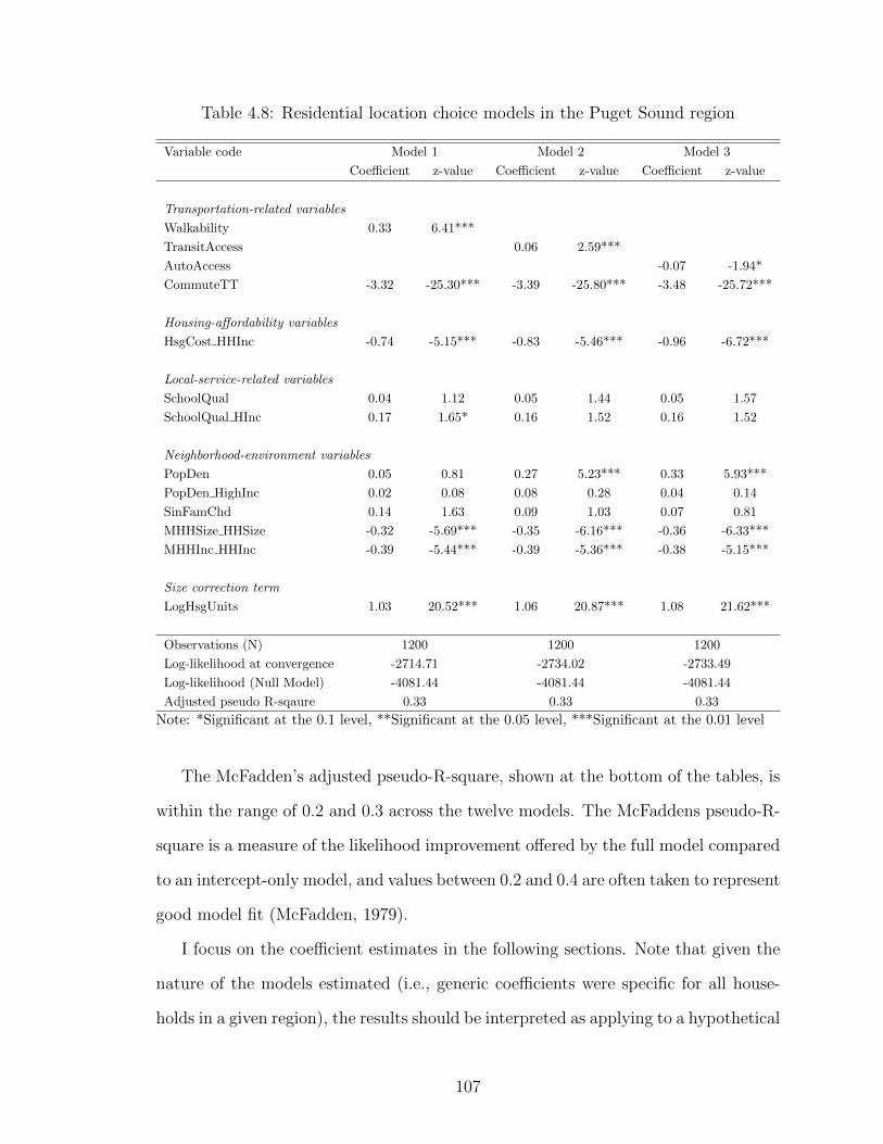
Table 4.8: Residential location choice models in the Puget Sound region
Variable code Model 1 Model 2 Model 3
Coefficient z-value Coefficient z-value Coefficient z-value
Transportation-related variables
Walkability 0.33 6.41***
TransitAccess 0.06 2.59***
AutoAccess -0.07 -1.94*
CommuteTT -3.32 -25.30*** -3.39 -25.80*** -3.48 -25.72***
Housing-affordability variables
HsgCost HHInc -0.74 -5.15*** -0.83 -5.46*** -0.96 -6.72***
Local-service-related variables
SchoolQual 0.04 1.12 0.05 1.44 0.05 1.57
SchoolQual HInc 0.17 1.65* 0.16 1.52 0.16 1.52
Neighborhood-environment variables
PopDen 0.05 0.81 0.27 5.23*** 0.33 5.93***
PopDen HighInc 0.02 0.08 0.08 0.28 0.04 0.14
SinFamChd 0.14 1.63 0.09 1.03 0.07 0.81
MHHSize HHSize -0.32 -5.69*** -0.35 -6.16*** -0.36 -6.33***
MHHInc HHInc -0.39 -5.44*** -0.39 -5.36*** -0.38 -5.15***
Size correction term
LogHsgUnits 1.03 20.52*** 1.06 20.87*** 1.08 21.62***
Observations (N) 1200 1200 1200
Log-likelihood at convergence -2714.71 -2734.02 -2733.49
Log-likelihood (Null Model) -4081.44 -4081.44 -4081.44
Adjusted pseudo R-sqaure 0.33 0.33 0.33
Note: *Significant at the 0.1 level, **Significant at the 0.05 level, ***Significant at the 0.01 level
The McFadden’s adjusted pseudo-R-square, shown at the bottom of the tables, is
within the range of 0.2 and 0.3 across the twelve models. The McFaddens pseudo-R-
square is a measure of the likelihood improvement offered by the full model compared
to an intercept-only model, and values between 0.2 and 0.4 are often taken to represent
good model fit (McFadden, 1979).
I focus on the coefficient estimates in the following sections. Note that given the
nature of the models estimated (i.e., generic coefficients were specific for all house-
holds in a given region), the results should be interpreted as applying to a hypothetical
107

average regional household rather than specific population groups. That is to say,
when a policy intervention (e.g., expansion of transit services) leads to changes in a
given variable (transit accessibility), the coefficients show the potential impacts on a
random group of households in the region rather than on a specific group of house-
holds. In practice, however, due to the existence of preference heterogeneity specific
population groups are more likely to respond to policy changes than a random group
of households; for example, individuals who have a stronger preference for transit ac-
cessibility are more likely to move into newly built transit-oriented development areas.
Therefore, the actual policy effects are likely to be larger than what the estimated
coefficients indicate.
Also, the estimated coefficients here were not regular coefficients butX-standardized
coefficients. They were obtained by fitting multinomial logit models on standardized
input data, i.e., each variable except LogHsgUnits was standardized by subtracting
its mean from each of its values and then dividing these new values by the standard
deviation of the variable. Like the standardized coefficients in regression analysis,
these X-standardized coefficients allow the modeler to directly assess the strength
of the effect of each independent variable on the choice outcome, and the variable
with the largest coefficient has the strongest influence. There is a notable difference
between regular standardized coefficients and the X-standardized coefficients used
here. Regular standardized coefficients were derived by standardizing both the X
and y variables. In logit models, however, only the X variables were standardized
because y, the utility of an alternative, is a latent utility variable unobserved to the
modeler. If one is only interested in the rank order of the magnitude of the effects
of the independent variables on the utility, however, X-standardization is sufficient
(Menard, 2004)
108

4.5.2 Control variables
In this section, I discuss the sign and statistical significance (at the 0.05 level) of
the coefficient estimates for the control variables (non-accessibility variables). Within
each region, the coefficient estimates barely differ across the three models that in-
cluded a different location-accessibility measure. Generally speaking, these coefficient
estimates are reasonable and consistent with the existing theoretical and empirical
evidence.
First of all, the coefficient of CommuteTT was negative and highly significant in
all twelve models, indicating a strong impact of commute time on housing decisions.
This finding was not new, since almost all previous studies on residential location
choice found the same (e.g., Lee et al., 2010; Levine, 1998). However, by estimating
residential location choice models with an identical model structure across three U.S.
regions with distinctive urban structures, my study confirms with robust empirical
evidence that CommuteTT remains a top consideration in household residential deci-
sions. In fact, the magnitude of the CommuteTT coefficient was the largest among all
independent variables, a finding similar to previous studies that used regional house-
hold travel survey data to examine the relative importance of different factors (Liu,
2012; Lee et al., 2010).
The housing affordability indicator, HsgCost HHInc, was negative and significant
at the 0.05 level across all twelve models. This suggests that households are less
likely to choose a zone which is less affordable to them. The school-quality vari-
ables, SchoolQual and SchoolQual HInc, were positive in most models (except that
SchoolQual was negative in the Southeast Michigan models), which indicate that
households, particularly the high-income ones with children, prefer to live in places
with access to good schools.
A crime-rate variable was incorporated into the Southeast Michigan-region models
(crime data were not available to me for Atlanta and Puget Sound), and it is negative
109

and highly significant. This finding confirms the conventional wisdom that safety
is a major consideration in housing decisions. Failing to include the crime variable
into the Atlanta and Puget Sound models would likely bias the estimates of other
independent variables that are correlated with crime rate. Since crime has a negative
impact on household residential location choice and accessibility variables are likely
to be positively correlated with crime rate, the coefficient estimates of CompactAcc,
Walkability, TransitAcc, AutoAccess in the Atlanta and Puget Sound models are likely
to have a downward bias.
Next are the neighborhood-environment related variables. In the Southeast Michi-
gan and Atlanta models, PopDen and PopDen HighInc were negatively associated
with residential location choice, which reflects the preference for low-density living
among the households living in these regions (Myers and Gearin, 2001). By contrast,
PopDen was positive and highly significant in the Puget Sound models. SinFam-
Chd had a positive coefficient across all models, confirming the conventional wisdom
that households with children tend to have a stronger preference for single-family
homes. Moreover, as suggested by the negative signs on MHHSize HHSize and MH-
HInc HHInc, there is strong neighborhood sorting by household characteristics and
household income.
Several race-related variables were specified in the Atlanta models but not the
Southeast Michigan and Puget Sound models because the ARC survey collected the
race information of the household members but the other two household surveys
did not. WtPctWt, BkPctBk, and AsPctAs had a positive sign, which suggests that
Whites, Blacks, and Asians tend to sort into neighborhoods of the same race. By con-
trast, HpPctHp had a negative but insignificant sign, meaning that Hispanics were
more likely to disperse into mixed-race neighborhoods. I also tested a model specifi-
cation without these race variables, and the coefficient estimates on the accessibility-
related variables did not change much. Therefore, while race-based sorting plays an
110

important role in residential decisions, without accounting for it may not create a
serious omitted variable bias problem for estimating the impact of accessibility on
residential location choice.
Finally, the coefficient on the size correction term, LogHsgUnits, was reasonably
close to unity and highly significant across all twelve models. Theoretically, this
variable should have a coefficient of one if all units of a particular type in a given
zone are truly homogeneous, a necessary condition underlying the assumption that a
zonal-level choice model can result in parameter estimates consistent with a housing-
unit level model (Lerman, 1975). Therefore, these coefficient estimates validated the
modeling of residential location choice at the TAZ level with a multinomial logit
model.
4.5.3 Accessibility variables
I now focus on the accessibility-related variables, which are the main variables of
interest. I mainly examine the sign and statistical significance (at the 0.05 level) of
their coefficients. I also compare the magnitude of the (X-standardized) coefficients
on accessibility variables with the control variables in order to assess their relative
influence on residential location choice.
Walkability
Two possible reasons may account for the difference in the coefficient estimates
of Walkability across regions. One is that households living in the Puget Sound re-
gion have a stronger preference for walkability than households in the Atlanta and
Southeast Michigan region. The other is that there is a great scarcity of walkable
neighborhoods (housing units) in Atlanta and Southeast Michigan; that is, if walka-
bility is a rare ”commodity”, most households simply do not or cannot actively seek
for it. The first argument attributes the results on Walkability to household pref-
erences whereas the second attributes them to the constraints they face, and both
111

preferences and constraints may explain individual choice outcomes.
Which of these two arguments is true have important implications on land use
and transportation policies. If the empirical evidence better supports the first argu-
ment, it means that compact-development efforts are less justifiable in the Atlanta
and Southeast Michigan region than in the Puget Sound region. To the least, the
implementation of compact-development initiatives is likely to face more oppositions
from the Atlanta and Southeast Michigan region residents than from the Puget Sound
Region residents. If the second argument is true, however, it suggests that the re-
vealed behavior (in terms of matching the preferences for walkability) in the Atlanta
and Southeast Michigan region may be the preferred behavior. That is to say, due
to the lack of choice, households in the Atlanta and Southeast Michigan region often
had to choose a residence with a lower level of accessibility than what they prefer. It
follows from this reasoning that compact development is warranted to expand choice
for households in the Atlanta and Southeast Michigan region (Levine et al., 2005).
Whether the regional differences in walkability’s coefficient estimates result from
household preference differences or market constraints is an empirical question. My
review of the relevant literature leads me to conclude that market constraints probably
play a greater role. My conclusion is based on the following observations. First, in a
study that compares the fit between people’s transportation and land-use preferences
(i.e., preferences for compact neighborhoods) and actual neighborhoods across the
Atlanta and Boston metropolitan areas, the researchers found that Boston allowed a
much closer fit than did Atlanta (Levine et al., 2005). They showed that Atlantans in-
deed have a relatively weaker preference for compact neighborhoods than Bostonians.
However, the difference in preferences is far from enough to explain why Atlantans
were much more likely to end up living in low-density, auto-dependent neighborhoods
than Bostonians, which suggests that the scarcity of compact development plays a
major role (Levine et al., 2005).
112

Table 4.9 presents the distribution of TAZs and housing units in terms of their
walkability level across three regions. These statistics clearly show that there is a
great scarcity of walkable neighborhoods—more accurately, a scarcity of housing units
locating in walkable neighborhoods—in the Atlanta and Southeast Michigan region
compared to the Puget Sound region. Only 3.2% and 4.3% of the housing units in
the Atlanta and Southeast Michigan region, respectively, were in the “very walkable”
category, compared to a 14.8% in the Puget Sound region. By contrast, 90.7% and
80.4% of housing units in the Atlanta and Southeast Michigan region respective were
in car-dependent neighborhoods, whereas only 72.2% of housing units in the Puget
Sound region were. Alarmingly, a large majority of housing units were built in car-
dependent neighborhoods, although surveys frequently report that only a minority
of American households prefer such neighborhoods (Levine et al., 2005; Frank et al.,
2019; Myers and Gearin, 2001).
Another piece of empirical evidence that leads support for the “market constraint”
view is the studies on how walkability affect property values. To my knowledge, almost
all of these studies found that walkability provided a significant boost to land and
property prices (Li et al., 2015; Bartholomew and Ewing, 2011; Pivo and Fisher,
2011). These studies were conducted in different cities, suggesting that walkability is
a desirable neighborhood attribute among the general population. This is evident in
the two regions themselves: in the Atlanta region, the redevelopment of the Beltline
that turns the surrounding areas into walkable and transit-accessible neighborhoods
has led to rapid property price increases (Immergluck and Balan, 2018); and in the
Southeast region, some walkable neighborhoods in downtown and midtown Southeast
Michigan have attracted many new businesses and residents in recent years (Riley,
2018).
The fact that walkability had a positively significant coefficient in almost all
hedonic-price regression models whereas it was insignificant in two of the three res-
113

Table 4.9: The distribution of walkability (across TAZs and housing units) in thethree regions
Atlanta Southeast Michigan Puget Sound
TAZ Housing units TAZ Housing units TAZ Housing units
Very walkable 4.5% 3.2% 5.6% 4.3% 21.3% 14.8%
Somewhat walkable 5.9% 6.2% 12.9% 15.3% 15.5% 13.0%
Car dependent 89.7% 90.7% 81.4% 80.4% 63.2% 72.2%
Note: Walk Score ranges from 0 to 100. A Walk Score of 70 and above is defined as very walkable,50 to 69 is somewhat walkable, and 49 and below is car-dependent.
idential location choice models is a subject that needs further study. I provide two
possible explanations here. One explanation is that the walkable neighborhoods in
the Puget Sound region are more desirable compared to the walkable neighborhoods
in the Atlanta and Southeast Michigan regions (see Figures 4.1, 4.2, and 4.3). This
can result from two factors. First, walkable neighborhoods in the Puget Sound re-
gion (mostly in the city of Seattle) are better designed (in terms of aesthetics and
pedestrian friendliness) than walkable neighborhoods in the Atlanta region (mostly
in downtown and midtown Atlanta) and in the Southeast Michigan region (mostly in
downtown and mid-town Southeast Michigan). Second, in the Atlanta and Southeast
Michigan region, housing quality is negatively associated with walkability (suburban
housing units are in general of better quality than urban housing units in these two
regions). Since housing quality is expected to be positively associated with residential
location choice and my models did not control for it, there is likely to be a downward
bias for the coefficient estimate on walkability.
The second explanation is that the alternative choice set that the modeler arbi-
trarily constructed for each household may not be the actual choice set considered
by that household. If neighborhoods of high walkability were included in the choice
set of households that in reality only considered auto-dependent neighborhoods when
deciding where to live, the coefficient estimates on walkability are likely to be biased
downward (Lerman, 1975). Given the scarcity of walkable neighborhoods in the At-
lanta region and the Southeast Michigan region, one can expect that walkability is
114

Map 4.1: The WalkScore of TAZs in the Atlanta region
Map 4.2: The WalkScore of TAZs in the Southeast Michigan region
115

Map 4.3: The WalkScore of TAZs in the Puget Sound region
considered by a small minority of households in their housing choice; however, neigh-
borhoods of high walkability were inevitably included into the choice set of most
households in the two regions since I had no information on if a household considered
walkability or not.
Transit accessibility
The estimated coefficients on transit accessibility were positive and statistically
significant at the 0.05 level in models across the three regions. While I am more
inclined to view this established relationship between transit accessibility and housing
choice as causal, there is also reason to believe that it is a pure correlation. The
“correlation” case can be supported by two main arguments. First, the data used
in my study are cross-sectional rather than longitudinal. Results of a cross-sectional
study are highly subjective to omitted variable bias and are commonly believed to be
116

insufficient to determine causal relationships. Second, there can be a reverse causality
issue. Transit lines and stops are usually located at high-density places to achieve the
goal of serving more people, that is to say, transit infrastructure (and hence transit
accessibility) may come after housing choice.
However, the case for “transit accessibility causing residential location choice” is
corroborated by two further pieces of empirical evidence. First, in surveys of residen-
tial preferences, households frequently indicated that transit access was an important
consideration (Chatman, 2009). People may value good transit access not only for
the actual use of the service but also for the opportunities it offers for unexpected
future use (Roson, 2001). Second, hedonic-price models generally estimate a positive
and significant impact of transit accessibility on property values. Scholarly inquiry
into how transit accessibility impacts land value and housing prices has existed for
decades, and the empirical evidence accumulated so far largely support the notion
that transit accessibility has a sizeable impact on property values (Mulley et al., 2016;
Knight and Trygg, 1977). For example, Armstrong and Rodriguez (2006) found that
properties located in municipalities with commuter rail stations were valued about
10% higher than properties in municipalities without a commuter rail station.
Auto accessibility
Auto accessibility had a negative coefficient in models across all three regions.
While a negative coefficient on auto accessibility was unexpected, previous studies
frequently reported the same (see, e.g., Guo and Bhat, 2007; Zolfaghari et al., 2012;
van de Vyvere et al., 1998). Previous studies often interpreted the negative sign as
suggesting that most people in the study area lived in neighborhoods of low auto
accessibility or that neighborhoods of high auto accessibility were often associated
with high levels of negative externalities (e.g., noise and traffic). Besides these reasons,
this may result from the fact that public roads are ubiquitous in U.S. metropolitan
117

regions and so the level of auto accessibility is sufficiently high at most locations. In
this context, households with cars would be indifferent to the variation in the level of
auto accessibility across locations. For households without cars, they are likely to be
even more indifferent since they cannot take advantage of auto accessibility anyway.
It should be noted that in separate models where I excluded the commute cost
variable (results not shown here), the coefficient on auto accessibility became positive
and statistically significant at the 0.05 level. This finding supports the construction
of more housing units at locations of high auto accessibility, in order to allow house-
holds that wish to cut commute costs to have more housing options (Levine, 1998).
Relative influence of accessibility on residential location choice
As discussed above, comparing the magnitude of the estimated X-standardized
coefficients can shed light on the relative influence of each variable on the choice
outcome. Across all three models, CommuteTT had the largest coefficient, suggesting
a very strong influence of commuting time on residential location choice. By contrast,
the magnitude of other accessibility indicators (i.e., overall accessibility, walkability,
transit accessibility, and auto accessibility) was relatively small, which ranked almost
at the bottom when compared with all other independent variables in terms of their
relative influence on residential location choice. One exception is the relative influence
of walkability in the Puget Sound region model, which ranked at the third place.
These findings are largely consistent with the results in several other resident location
choice studies that examined the relative influence of each independent variable on
the choice outcome (Lee et al., 2010; Liu, 2012).
4.6 Implication and discussion
These findings have important implications for land use and transportation plan-
ning practice and policymaking. First, the different impacts of walkability, transit
118

accessibility, and auto accessibility on residential location choice shed light on the
design of land use and transportation policies to promote accessibility. In addition,
the differences in model results across regions reveal that accessibility evaluation is
highly dependent on the regional context. Finally, the study calls into question the
existing long-term land use and travel models that are calibrated based on revealed
location- and travel-choice behavior, since revealed behavior is shaped by the existing
choice constraints and it can be different from preferred behavior.
4.6.1 The design of accessibility-promoting policies
The finding that transit accessibility exerts a significant influence on residential
location choice suggests that transit accessibility is a highly desirable attribute among
many households across U.S. regions. This finding explains the increases in housing
price in areas adjacent to transit infrastructure (Bowes and Ihlanfeldt, 2001) and
also provides empirical support for the planning practice of promoting more transit-
oriented developments in order to meet the market demand (Levine et al., 2005). In
addition, since transit accessibility is the only type of accessibility that has a positive
and significant coefficient across all three regional models, policies that promote tran-
sit accessibility are more likely to have a significant influence on residential patterns
than measures that promote walkability and auto accessibility. However, one should
not interpret this finding as suggesting that local residents are more supportive of
policies that promote transit accessibility than policies that promote walkability and
auto accessibility, since my models examine how households react to the level of dif-
ferent types of accessibility already available at different locations rather than how
they react to proposals to enhance accessibility. Such policy proposals usually come
with a cost and thus requires a different cost-benefit analysis in order to assess their
relative merits and disadvantages (Levine et al., 2018).
After controlling for commuting cost, households across all three regions do not
119

value auto accessibility in residential location choice (in fact, auto accessibility has a
negative coefficient). As I discussed above, this finding is not surprising: The com-
parative advantage and the relative attractiveness of a location depend on if it offers
a much higher level of accessibility than other locations; and in many U.S. regions
where there is almost ubiquitous road access across all locations, it is reasonable for
the locational advantage of central locations in auto accessibility to be perceived as
unimportant. This suggests that road investments are likely to have a relatively small
influence on location patterns in an environment of ubiquitous road access. On the
other hand, the finding that commuting cost is a highly significant factor across all
models provides empirical support for policy measures (e.g., job-housing balance) that
seek to reduce commuting cost. This contradicts an earlier claim which asserts that
commuting cost plays a decreasing role on household residential decisions and that
the land-use and transport link is weakening (Giuliano and Small, 1993; Giuliano,
1995).
The limited influence of auto accessibility on residential location choice should
nonetheless not be interpreted as suggesting that auto accessibility is not an important
and desirable location attribute. Beyond shaping location choice and development
patterns, land use and transportation planning policies and practices that promote
auto accessibility can result in other desirable social outcomes such as reduced vehicle
miles travelled (Ewing and Cervero, 2001), higher economic growth (Banister and
Berechman, 2001), and better employment prospects (Ihlanfeldt and Sjoquist, 1991).
When planning for the future, promoting auto accessibility—as opposed to promoting
automobility—should still be a fundamental planning goal (Martens, 2016; Levine
et al., 2019). A region that is experiencing decreasing auto accessibility would have
a lower level of attractiveness to potential future comers and lose in competitiveness
compared to other regions.
120

4.6.2 The importance of regional context in accessibility evaluation
A comparison of the similarities and differences of the model outputs across re-
gions can generate valuable insights on how regional context influences accessibility
evaluation in residential location choice modeling. Since the models specified in this
study have almost identical sets of independent variables and the measurement of
accessibility indicators (and most other variables) are the same, this study provides
robust empirical evidence (by ruling out the influences of model specification and
measurement) to understand how regional context matters. Nonetheless, I also bring
into discussion findings from other studies in order to have a more comprehensive
understanding of the generalizability of findings in this study.
The finding that transit accessibility has a significant impact on residential loca-
tion choice across all three regions is also consistent with most previous studies (e.g.,
Olaru et al., 2011; Hu and Wang, 2017).9. This means that one can comfortably
generalize this finding to other locations. Regarding auto accessibility, this study
shows that it has a negative coefficient in the models of all three regions, which indi-
cate a limited influence of auto accessibility on household location decisions. While
this finding is not uncommon, this finding contrasts with many other studies that
reported a positive and significant impact of auto accessibility on residential location
choice (e.g., Lee et al., 2010; Srour et al., 2002) While this difference may result from
differences in model specifications and measurements, regional context is also likely
to play a role. The regions studied here are all large U.S. metropolitan regions with
an extensive built-out area that is full of self-contained suburbs and an extensive road
network that well connects the region. This means that a household with access to
personal vehicles can enjoy a very high level of auto accessibility (accessibility to over
millions of job with an hour drive) at most locations. Since the marginal benefit that
9It should be noted, however, most previous studies use a distance-based accessibility (e.g.,distance to transit stop) rather than the more comprehensive gravity-based accessibility measureused here.
121

a household gains from additional accessibility increases at a high level of accessibility
is likely to be low (due to a decreasing marginal utility of accessibility), a household
may place little value on locations with higher auto accessibility. If the study area is
a smaller region with a much lower level of overall auto accessibility, it is likely that
households would value locations of higher auto accessibility more.
An intriguing finding of this study is that walkability was highly significant in the
Puget Sound region model but not significant in the Atlanta and Southeast Michigan
region. As I discussed above, this is most likely because there is a great under-supply
of walkable neighborhoods, particular walkable neighborhoods with better housing
quality and urban design, in the Atlanta and Southeast Michigan region. This under-
supply results in a lack of choice, causing most households living in these two regions
to be unlikely to consider walkability as an important factor when deciding where
to live. To my knowledge, walkability has not been incorporated into the residential
location choice models of previous studies, although existing residential preference
surveys often show that many residents view walkability to be important (Schwanen
and Mokhtarian, 2004; Urban Land Institute, 2015; Canadian Home Builders As-
sociation, 2015; Frank et al., 2019). Therefore, my study fills an important gap in
understanding the role of walkability in residential location choice modeling.
The findings on walkability in this study is consistent with another important
study that examines the degree to which residents in Boston and Atlanta are able
to translate their residential preference for walkable and transit-accessible neighbor-
hoods into their actual residence choice (Levine et al., 2005). In this study, Jonathan
Levine and his co-authors found that Boston—by providing a greater range of neigh-
borhood types—allowed a closer fit between household neighborhood preference and
the actual neighborhood choice than Atlanta. The major improvement of my study
to the Levine et al. study is that my residential choice models control for a range
of other factors such as housing affordability, local services, and neighborhood char-
122

acteristics, which greatly mitigates the omitted-variable-bias concern associated with
the model specified in the Levine et al. study. Together with the Levine et al. study,
my study highlights the importance of regional supply factors in shaping residential
location decisions and the valuation of accessibility in the process. From a policy
perspective, findings of both studies suggest the need for increasing the supply of
walkable and transit-accessible neighborhoods—for example, through the relaxation
of zoning regulations (Levine, 2006)—to allow households to have more choice in
housing decisions.
4.6.3 A need to incorporate “preferred” behavior in integrated land use
and transport modeling
The residential location choice models implemented in this study are standard
models used in an integrated land use and transportation modeling procedure (Wad-
dell, 2002), which was conducted by metropolitan planning agencies to guide land
use/transportation investments and decisions. In the process, residential location
choice models are used to predict the distribution of population growth, usually in
the next twenty or thirty years, in different parts of the region. As is the case in this
study, the main data source for residential location modeling is the regional household
travel survey.
Results of my study point to a potential issue with the current standard practice.
The issue is that residential location choice prediction is only based on the revealed
behavior of regional households, which is necessarily constrained by the existing mar-
ket and individual constraints and thus may not be the preferred behavior (Handy and
Niemeier, 1997). As I have discussed above, the coefficient estimates on walkability—
for the Atlanta and Southeast Michigan region—do not indicate that residents in the
Atlanta and Southeast Michigan region do not value walkable neighborhoods, but
rather suggest that they are not able to choose walkable neighborhoods due to the
123

lack of choice. These households may well consider moving to a more walkable neigh-
borhood if more walkable neighborhoods with better schools and local services are
built in the future and thus bring a greater diversity of choice.
However, a standard application of the residential location choice models in the
Atlanta and Southeast Michigan regions, which assumes that the model outputs re-
flect the preferences of future residents, would signal to planners and policymakers
that households in the two regions do not value walkability and thus the provision
of walkable neighborhoods is unwarranted. Also, since the outputs of a residential
location choice model are inputs the subsequent travel-demand models, an under-
prediction of population growth in walkable neighborhoods would lead the modelers
to predict less nonmotorized trips. When the predicted future travel is used to guide
transportation investments and decisions, more resources are likely to be diverted to
motorized travel at the expense of undermining nonmotorized travel. This practice
thus constitutes another form of the “predict and provide” approach in transportation
planning that has been widely criticized in recent decades (Kenworthy, 2012).
Therefore, I argue that residential location choices with prediction purposes (e.g.,
when performing as a component of integrated land use-transport model systems)
should incorporate both information regarding the preferred behavior of households
and also their revealed behavior at present. One possible approach to achieve this can
be adding some stated-preference questions in the existing regional household travel
surveys, and incorporate such information into the land use and transport modeling
procedure. Research on joint modeling of revealed-preference and stated-preference
data has been ongoing for decades, which has been widely applied in travel modeling
(e.g., Ben-Akiva and Morikawa, 1990) but much less so in location choice modeling.
124

4.7 Conclusion
In recent years, there are two major debates in the planning literature related
to accessibility: one is the debate on the desirability of compact development ver-
sus sprawled growth (Ewing, 1997; Gordon and Richardson, 1997), and the other
is accessibility-based versus mobility-based transportation and land use planning
(Cervero, 1997; Salomon and Mokhtarian, 1998; Levine et al., 2019). These nor-
mative debates are still ongoing but the scale is gradually shifting toward the di-
rection of accessibility, with accessibility and its corresponding policies gaining more
and more support among researchers and making inroads into planning practices
(Boisjoly and El-Geneidy, 2017; Proffitt et al., 2019). A much less discussed and
less well-understood topic, however, is how to plan for accessibility; specifically, little
knowledge is available regarding which types of accessibility to prioritize when plan-
ners and policymakers establish the goals of transportation and land use planning.
This study fills this gap by examining how regional households value walkabil-
ity, transit accessibility, and auto accessibility differently in their residential location
choice. To further evaluate the generalizability of study findings and to investigate
how regional context matters for accessibility valuation in household residential deci-
sions, I fit residential location choice models for random samples of households living
in three U.S. regions, namely, the Atlanta region, the Puget Sound region, and the
Southeast Michigan region. Since accessibility is a “good” with many proven benefits,
in theory, they should all have a positive influence on household residential location
choice. The model outputs only partially confirm this notion. The results show that
transit accessibility has a significant influence on household residential location choice
across all regions. Walkability is an important determinant of residential location for
the Puget Sound households, but not for the Atlanta and Southeast Michigan house-
holds. Somewhat surprisingly, auto accessibility, perhaps the type of accessibility
mostly discussed and measured among the three, appears to have little influence on
125

residential location decisions.
The valuation of accessibility in residential location choice is jointly determined
by two major factors: the preferences of local residents (i.e., demand factor), and
the supply of different types of accessibility in the regional housing stock. However,
previous studies on residential location choice have generally interpreted the model
outputs as an indication of resident preferences while ignoring the potential influences
of the supply factors. That is to say, if the coefficient of an accessibility indicator
is statistically insignificant, it would be interpreted as suggesting that residents do
not have a strong preference for it when deciding where to live. The findings of my
study suggest that this interpretation can be erroneous. I argue that the insignificant
coefficients on walkability in the Atlanta and Southeast Michigan models are more re-
flective of the scarcity of walkable neighborhoods in these two regions rather than the
fact that households in the two regions do not value walkability as much as households
in the Puget Sound region. Likewise, the limited influence of auto accessibility on res-
idential decisions across all three regions is better interpreted as suggesting that the
ubiquity of road access evens out the accessibility differences across locations instead
of suggesting that auto accessibility are not important.
My study also has important implications for land-use and transportation plan-
ning practice and policymaking. First of all, it appears that for U.S. regions, policy
measures that promote transit accessibility are more likely to shape residential lo-
cation outcomes than measures that promote walkability and auto accessibility. In
fact, new road investments are likely to have a minimal influence on residential lo-
cation patterns considering an environment of ubiquitous road access in major U.S.
metropolitan regions. These findings are supported by the model outputs in all three
regions, which ensure a high degree of generalizability to other large metropolitan
regions. The results on auto accessibility are less transferable to smaller regions,
however, because the absolute level of auto accessibility is lower (accessibility is likely
126

to be valued more at a lower absolute level due to decreasing return in utility) and
the road infrastructure is likely to be less pervasive. Moreover, the fact that walka-
bility has a varying degree of influence on household residential decisions across the
three regions highlights the importance of regional context in accessibility valuation.
Whereas households in the Puget Sound region can enjoy a better fit between their
residential preferences for walkability and actual neighborhood choice, the scarcity
of walkable neighborhoods in the Atlanta and Southeast Michigan region often force
households in the two regions to live in less walkable neighborhoods in order to satisfy
other needs such as good schools and good municipal services. This finding suggests
the need for increasing the supply of walkable neighborhoods (such as by relaxing
zoning regulations) to expand the choice of walkability-preferring households.
Finally, this study call for a need to incorporate information regarding the “pre-
ferred behavior” of households into land use and transportation modeling. The ex-
istence of market constraints means that people’s actual choice may not be their
desired choice, and so there is often a disparity between revealed behavior and pre-
ferred behavior. This means that a sole reliance on revealed-behavior data for land
use and transportation modeling, whose outputs are consequently used to guide land
use and transportation planning, can lead to future scenarios that reinforce the status
quo, which are most likely to be very different from the preferred scenario of local
residents. Eliciting information regarding households’ preferred behavior and incor-
porating it into the process of land use and transportation planning can thus lead to
better policy prescriptions and planning outcomes.
127

CHAPTER V
Conclusion
Access is a basic human need. People need access to other people: to family
and relatives, to friends, to potential mates, to business partners, and to a variety
of casual acquaintances. They also need access to activities, goods, services, and
natural amenities, such as to job opportunities, food, medical services, and parks or
other recreational sites.
These needs in turn shape individual residential location and travel decisions.
When people decide where to live, an important factor they consider is the level of
accessibility a location offers, that is, the convenience/potential from it to reach desir-
able destinations (i.e., people and opportunities) distributed across space. Everything
else being equal, individuals in general would prefer a site that offers a higher level of
accessibility to work and nonwork destinations because it provides them more choices
when making travel decisions. By determining the price of travel from a location
to potential destinations (Boarnet and Crane, 2001), accessibility shapes individual
travel decisions regarding how many trips to take, which destinations to visit, and
which travel modes to use and at what frequency.
Land-use and transportation planning shapes the spatial distribution of people
and activities (i.e., land-use patterns) and the ease of travel between them (i.e., the
transport system), the two major components of accessibility.1 Thus to enhance indi-
1Geurs and Van Wee (2004) decomposed accessibility into four components: land use, trans-
128

vidual residential and travel satisfaction, an intuitive approach is to promote land-use
and transportation planning policy and practice that can enhance accessibility. Ac-
cessibility improvements can come from either land-use policies such as new urbanism,
mixed-use development, and job-housing balance that promote the proximity between
origins and destinations or transportation policies such as travel-demand management
and rail investments that promote travel speed (Grengs et al., 2010; Levine et al.,
2012). Nevertheless, proximity-enhancing policies such as job-housing balance and
transit-oriented development (often jointly referred to as “compact development” or
“smart growth”) have been heatedly debated in recent decades.
Up until the early 2000s, a major focus of the debate is whether compact-development
policies are justifiable on the basis of free-market principles. While critics of compact
development assert that the prevailing low-density, auto-dependent development pat-
terns (urban sprawl) across the U.S. is a result of market forces and an expression
of consumer preferences (Gordon and Richardson, 2001, 1997; Glaeser and Kahn,
2004), supporters argue that urban sprawl results from both market failures (Ewing,
1997; Brueckner, 2000) and planning failures (Levine, 2006). Major market failures
associated with urban growth include a failure to account for the benefits of open
space, a failure to account for the social costs of driving, and a failure to make new
development pay for the infrastructure costs it generates (Brueckner, 2000). And
the planning failure lies in the inadequate supply of walkable and transit-friendly
neighborhoods that households prefer due to the pervasive single-family, exclusionary
zoning practices (Levine and Inam, 2004; Levine et al., 2005; Levine, 2006). The
debate on compactness-versus-sprawl has cooled down in recent years, with a grow-
portation, temporal, and individual. The temporal component distinguishes accessibility by timeof the day or day of the week (Miller, 1991; Kwan, 1998; Miller, 1999), which can be captured bythe land-use and transport components if the “operating” hours of activities (e.g., business hours ofstores) and transportation services (e.g.. operating hours of transit services) are accounted for. Theindividual component further accounts for individual preferences, needs, and constraints; however,the focus of this dissertation is on location accessibility (i.e., place-based accessibility) instead ofpeople-based accessibility.
129

ing majority of scholars recognize the inefficiency, environmental harms, and social
inequality associated with sprawl (Anderson et al., 1996; Johnson, 2001; Owen et al.,
2004; Clifton et al., 2008).
More recent debates on accessibility-promoting land-use and transportation poli-
cies center on if these policies are effective tools to achieve planning goals such as
reducing car use (Ewing and Cervero, 2010; Stevens, 2017) and whether or not acces-
sibility remains to be an important locational factor in an era of declining transport
costs (Glaeser and Kohlhase, 2004). Naturally, evidence showing that accessibility
significantly affects travel behavior (e.g., reduce driving or promote the use of non-
motorized modes) and shapes locational decisions supports these policies, whereas
the absence of significance influences undermines the rationale for accessibility-based
planning policymaking and practice. The existing empirical evidence on these top-
ics is extensive but mixed. While many researchers have argued that accessibility-
promoting compact-development policies can reduce car use (Cervero and Kockelman,
1997; Ewing and Cervero, 2001, 2010) and that accessibility is a main determinant of
residential location choice (Lee et al., 2010; Hu and Wang, 2017; Baraklianos et al.,
2018), other scholars have questioned the merits of accessibility-promoting policies;
they argue that these policies do not necessarily reduce driving and traffic congestion
(Crane, 1996a,b; Salomon and Mokhtarian, 1998; Mokhtarian and Salomon, 2001) or
that accessibility is playing a declining role in shaping household residential decisions
(Giuliano, 1995).
The capacity of research to support or reject the merits of accessibility is greatly
influenced by the empirical measures of accessibility benefits. In both the residential-
location choice and travel-behavior studies, researchers have mainly relied on mea-
sures of travel-cost savings (TCS) to represent the benefits of accessibility. In the
residential location choice context, the measures are commuting-cost savings or re-
duced household travel expenditure; and in the travel-behavior context, they are
130
reduced vehicle-mile-traveled (VMT) reduction or decreases in the contributing fac-
tors of VMT such as trip frequency, trip length, or the probability of driving. In other
words, these studies have applied TCS as the main criterion to evaluate accessibility-
enhancing land-use and transportation policies. And researchers have often cited the
absence of significance TCS to question the merits and importance of these policies
(Hamilton and Roell, 1982; Giuliano, 1995; Crane, 1996b; Stevens, 2017; Smart and
Klein, 2018a).
In this dissertation, I have argued that a TCS-based accessibility policy evaluation
ignores the non-TCS aspects (i.e., destination-utility gains) of accessibility benefits,
which underestimates the value of accessibility and hence without basis weaken the
policy importance of accessibility-promoting strategies. This argument is supported
by both theoretical reasoning and empirical evidence. Based on data collected from
the Puget Sound and Southeast Michigan region, I find that transit accessibility re-
mains to have a significant impact on residential location choice after controlling
for all TCS associated with, which I interpret as suggesting that individuals de-
rive destination-utility gains (mainly option value) from transit access. A search for
destination-utility gains often motivates individuals to make more trips and/or to
travel to more remote (and more desirable) destinations, which in turn induces addi-
tional car travel; this travel-inducing effect was verified by the trip-frequency models
estimated in the Southeast Michigan region, which show that transit accessibility was
positively associated with car-trip frequency.
In fact, that the economic value of accessibility is beyond travel-cost savings has
long been recognized by a branch of the urban and regional economics literature that
concerns agglomeration economies, which refers to the positive externalities that in-
dividuals and firms gain from accessing to nearby individuals and firms (Marshall,
1890). While the classic urban and regional economics theories such as the firm-
location theory (Weber, 1909), central place theory (Christaller, 1933; Losch, 1940),
131

and regional economy (Isard, 1956) were all built on transportation costs, in re-
cent decades economists have increasingly relied on the concept of agglomeration
economies to explain the concentration of activities in metropolitan areas and urban
centers (Fujita and Ogawa, 1982; Lucas Jr et al., 2001; Glaeser, 2010). The main
mechanisms of agglomeration economies include labor pooling, input sharing, and
knowledge spillovers (Duranton and Puga, 2004).
The theory of agglomeration economies is well known, but its connection with
accessibility research is not well understood.2 Existing research tends to examine
agglomeration economies at the city-level or regional-level, without distinguishing
the intraurban differences (Duranton and Puga, 2004; Rosenthal and Strange, 2004).
In recent years, however, a limited number of studies have sought to incorporate a
consideration of the production externalities available at different locations into the
modeling of urban spatial structure (Fujita and Ogawa, 1982; Imai, 1982; Lucas Jr
et al., 2001; Allen et al., 2015), and the location-production functions applied in these
studies can be essentially thought as a type of accessibility measure. This means that
accessibility can also be thought of as an indicator of agglomeration economies. By
establishing this connection in this dissertation, I not only add theoretical depth
to the argument that accessibility has benefits beyond travel-cost savings but also
bridges two large and disconnected bodies of literature—land-use and transportation
research and agglomeration economies.
A marriage between two bodies of literature generates valuable insights for ur-
ban research and policymaking. For example, the fact that agglomeration economies
operate in the form of production externalities provides a rationale for government in-
tervention to promote overall regional accessibility. For example, as Anas et al. (1998)
suggests, the inability of economic actors to internalize agglomeration economies can
prevent the free market to form optimal urban spatial structure, which thus opens
2Exceptions include a few recent studies have empirically established the link between accessi-bility and labor productivity (Chatman and Voorhoeve, 2010; Melo et al., 2017).
132

the door for government interventions such as assisting sub-center formation by pro-
viding infrastructure or relaxing the land-use regulations. This is in line with what
land-use and transportation planners have argued for—establishing accessibility as a
central goal of social policymaking (Wachs and Kumagai, 1973; Cervero, 1997; Levine
et al., 2019). Notably, this efficiency-based rationale (i.e., addressing externalities)
adds further theoretical underpinning to the promotion of accessibility as a major
planning goal.
My dissertation also opens the door for a new direction of accessibility research
to investigate the nature and magnitude of destination-utility gains. The empirical
work presented here is tentative and preliminary steps to verify its existence and its
influence on residential location and travel decisions. As I have discussed in the body
of the work, an ideal empirical approach to destination-utility gains requires the use
of longitudinal data that records the behavioral changes of individuals who experi-
ence accessibility gains. I have resorted to cross-sectional data here due to resource
constraints, which is a major limitation of my work. Future work should address this
limitation. In addition, future work should examine how different population groups
value travel-cost savings and destination-utility gains differently, which can generate
insights which population groups to target when specific policy goals are set. For
example, an understanding of which population groups have a stronger preference for
destination-utility gains can inform policymakers with VMT-reduction goals to avoid
targeting areas with large concentrations of these population groups.
On planning policy and practice, findings of this dissertation highlight the need
to shift from a TCS-based to an accessibility-based land-use and transportation
policy evaluation. Until now, the destination-utility aspects of accessibility have
rarely been discussed or even mentioned in planning-related discussions, whether it
is an infill-development project or a transit-investment proposal. To better promote
accessibility-based planning strategies, planners should stress to policymakers and
133

the general public the various forms of destination-utility gains, such as the choice
value derived from greater flexibility and variety, enhanced social and economic in-
teractions, and the associated spillover effects such as knowledge transfer and social
learning. These arguments would be further strengthened if the regional household
travel survey incorporates questions regarding individual preference for various forms
of destination-utility gains and if empirical indicators of these destination-utility gains
are incorporated into the land-use and transportation plans developed by metropoli-
tan planning organizations.
Moreover, standard tools of transportation planning, such as traffic-impact anal-
ysis and level-of-service modeling, are based strictly in a mobility paradigm. An
expanded accessibility view as outlined here highlights the urgency of shifting from
mobility to accessibility as the basis for prospective and retrospective planning evalu-
ation. While a shift in the evaluative tools does not equate to changes in the physical
environment, such a shift can remove impediments to on-the-ground accessibility-
based planning implementation. As I have noted in chapter two, the recent integrated
land-use and transport models have already modeled accessibility with more compre-
hensive measures (e.g., gravity-based and utility-based measures) that can capture
both the TCS and destination-utility gains. By elaborating on the different types
of economic benefits picked up by these measures, My dissertation thus provides a
theoretical underpinning to the accessibility modeling approach in these models.
My dissertation further contributes to planning practice by identifying a major
methodological flaw in existing land-use and transportation modeling and simulation
work. When metropolitan planning organizations calibrate regional land-use and
transportation models to forest future land-use patterns, they usually rely on current
or historical data on household travel and residential location behavior to estimate
household preference for accessibility. These preference estimates are then directly
applied to the forecasting models. Chapter 4 of the dissertation shows that such
134

practice is problematic because households’ revealed behavior, which these preference
estimates are derived from, is often different from their “preferred behavior” because
of the existence of supply constraints. These constraints prevent them from express-
ing their true preferences, which implies that solely relying on revealed behavior for
land-use and transportation modeling can exaggerate the problematic “predict-and-
provide” transportation-modeling approach that has been heavily criticized in the
literature (Owens, 1995; Banister). Therefore, I argue that land-use and transport
models with predictive purposes should incorporate information regarding the pre-
ferred behavior of households.
Written at a time when fully automated vehicles will soon (at least according
to optimistic predictions) pour into our streets, this dissertation sheds light on the
question of how autonomous vehicles will shape individual residential-location and
travel patterns. Autonomous vehicles free people from driving and allow them to
work, entertain, or rest in the car, which means that the disutility associated with in-
vehicle travel time would decrease significantly. That is to say, autonomous vehicles
will lead to substantive reductions in the time cost of travel perceived by travelers. As
the time-plus-money cost of travel declines, individual travel and residential-location
decisions are likely to be less driven by travel-cost savings than the competing factors
(e.g., neighborhood quality in the context of residential location choice). Thus under
a TCS-based view of accessibility benefits, geographical proximity between people and
activities would become less important in an era of autonomous vehicles; individuals
are likely to live further away from their jobs and would be more willing to take long
trips. It follows that autonomous vehicles would lead to further suburban sprawl and
greater VTM consumption.
While I do not negate these potential impacts, I stress here the existence and
importance of destination-utility gains, another form of accessibility benefits that
can hold people and activities together in an era of autonomous vehicles. While
135

autonomous vehicles are expected to reduce the TCS associated with proximity, they
are less likely to reduce the interaction value (a component of destination-utility gains
as I described in chapter two) brought by it. Holding the transport network constant,
greater proximity to spatially distributed opportunities (i.e., people and activities)
leads to more interactions within a given amount of time. Any additional minute
spent on travel, in either an autonomous vehicle or a regular car, means lost time
and potential opportunity for meaningful interactions. Therefore, if people live too
far away from work or take longer trips, they would be able to make fewer trips
(purposeful interactions) in a given day; and if people are far away from other people
and activities, they are less likely to gain from random interactions, i,e,, knowledge
spillovers (Jaffe et al., 1993) and social learning (Glaeser, 1999). Therefore, under
emerging technologies, as with the transportation and communication technologies of
the past, it remains important for us to build cities and regions that facilitate better
accessibility.
136

BIBLIOGRAPHY
137

BIBLIOGRAPHY
Adair, A., McGreal, S., Smyth, A., Cooper, J., and Ryley, T. (2000). House prices andaccessibility: The testing of relationships within the belfast urban area. Housingstudies, 15(5):699–716.
Ahlfeldt, G. (2011). If alonso was right: modeling accessibility and explaining theresidential land gradient. Journal of Regional Science, 51(2):318–338.
Allen, T., Arkolakis, C., and Li, X. (2015). Optimal city structure. Working paper.
Alonso, W. (1960). A theory of the urban land market. Papers in Regional Science,6(1):149–157.
Alonso, W. (1964). Location and land use. Toward a general theory of land rent.Harvard University Press, Cambridge, Massachusetts.
Anas, A. (1982). Residential Location Markets and Urban Transportation. EconomicTheory, Econometrics and Policy Analysis With Discrete Choice Models. NewYork: Academic Press.
Anas, A., Arnott, R., and Small, K. A. (1998). Urban spatial structure. Journal ofeconomic literature, 36(3):1426–1464.
Anderson, W. P., Kanaroglou, P. S., and Miller, E. J. (1996). Urban form, energy andthe environment: a review of issues, evidence and policy. Urban studies, 33(1):7–35.
Armstrong, R. J. and Rodriguez, D. A. (2006). An evaluation of the accessibility bene-fits of commuter rail in eastern massachusetts using spatial hedonic price functions.Transportation, 33(1):21–43.
Audirac, I. (1999). Stated preference for pedestrian proximity: an assessment ofnew urbanist sense of community. Journal of Planning Education and Research,19(1):53–66.
Banister, D. Transport planning. In Button, K. and Hensher, D., editors, Handbookof transport systems and traffic control.
Banister, D. and Berechman, Y. (2001). Transport investment and the promotion ofeconomic growth. Journal of transport geography, 9(3):209–218.
138

Baraklianos, I., Bouzouina, L., Bonnel, P., and Aissaoui, H. (2018). Does the ac-cessibility measure influence the results of residential location choice modelling?Transportation, pages 1–30.
Bartelme, D. (2015). Trade costs and economic geography: evidence from the us.Working Paper, University of California, Berkeley.
Bartholomew, K. and Ewing, R. (2011). Hedonic price effects of pedestrian-andtransit-oriented development. Journal of Planning Literature, 26(1):18–34.
Ben-Akiva, M. and Bowman, J. L. (1998). Integration of an activity-based modelsystem and a residential location model. Urban Studies, 35(7):1131–1153.
Ben-Akiva, M. and Lerman, S. (1979). Disaggregate travel and mobility choice modelsand measures of accessibility. In Hensher, D. and Stopher, P., editors, BehavioralTravel Modeling, pages 654–679. London: Croom Helm.
Ben-Akiva, M. and Morikawa, T. (1990). Estimation of switching models from re-vealed preferences and stated intentions. Transportation Research Part A: General,24(6):485–495.
Blumenberg, E. and Pierce, G. (2012). Automobile ownership and travel by the poor:Evidence from the 2009 national household travel survey. Transportation ResearchRecord, 2320(1):28–36.
Blumenberg, E. and Pierce, G. (2017). Car access and long-term poverty exposure:Evidence from the moving to opportunity (mto) experiment. Journal of transportgeography, 65:92–100.
Boarnet, M. and Crane, R. (2001). The influence of land use on travel behavior:specification and estimation strategies. Transportation Research Part A: Policyand Practice, 35(9):823–845.
Boarnet, M. G. (2011). A broader context for land use and travel behavior, and aresearch agenda. Journal of the American Planning Association, 77(3):197–213.
Boarnet, M. G. and Wang, X. (2019). Urban spatial structure and the potentialfor vehicle miles traveled reduction: the effects of accessibility to jobs within andbeyond employment sub-centers. The Annals of Regional Science, 62(2):381–404.
Boisjoly, G. and El-Geneidy, A. M. (2017). How to get there? a critical assessment ofaccessibility objectives and indicators in metropolitan transportation plans. Trans-port Policy, 55:38–50.
Bonavia, M. R. (1936). Economies of transport. Nisbet and Co LTD, London.
Bowes, D. R. and Ihlanfeldt, K. R. (2001). Identifying the impacts of rail transitstations on residential property values. Journal of Urban Economics, 50(1):1–25.
139

Bristow, A. and Nellthorp, J. (2000). Transport project appraisal in the europeanunion. Transport policy, 7(1):51–60.
Brown, B. B. and Cropper, V. L. (2001). New urban and standard suburban subdivi-sions: Evaluating psychological and social goals. Journal of the American PlanningAssociation, 67(4):402–419.
Brueckner, J. K. (2000). Urban sprawl: diagnosis and remedies. International regionalscience review, 23(2):160–171.
Brueckner, J. K. et al. (1987). The structure of urban equilibria: A unified treatmentof the muth-mills model. Handbook of regional and urban economics, 2(20):821–845.
Burns, L. D. and Golob, T. F. (1976). The role of accessibility in basic transportationchoice behavior. Transportation, 5(2):175–198.
Campbell, S. (1996). Green cities, growing cities, just cities?: Urban planning andthe contradictions of sustainable development. Journal of the American PlanningAssociation, 62(3):296–312.
Canadian Home Builders Association, p. (2015). Home buyer preference survey. Tech-nical report, Ottawa: Canadian Home Builders Association.
Cao, X., Mokhtarian, P. L., and Handy, S. L. (2009). Examining the impacts of resi-dential self-selection on travel behaviour: a focus on empirical findings. Transportreviews, 29(3):359–395.
Cascetta, E., Cartenı, A., and Montanino, M. (2016). A behavioral model of ac-cessibility based on the number of available opportunities. Journal of TransportGeography, 51:45–58.
Cervero, R. (1997). Paradigm shift: from automobility to accessibility planning.Urban Futures (Canberra), (22):9–20.
Cervero, R. and Hansen, M. (2002). Induced travel demand and induced road in-vestment: a simultaneous equation analysis. Journal of Transport Economics andPolicy (JTEP), 36(3):469–490.
Cervero, R. and Kockelman, K. (1997). Travel demand and the 3ds: Density, diversity,and design. Transportation Research Part D: Transport and Environment, 2(3):199–219.
Cervero, R. and Wu, K.-L. (1997). Polycentrism, commuting, and residential locationin the san francisco bay area. Environment and Planning A, 29(5):865–886.
Chapple, K. and Loukaitou-Sideris, A. (2019). Transit-Oriented Displacement orCommunity Dividends?: Understanding the Effects of Smarter Growth on Com-munities. MIT Press.
140

Chatman, D. and Voorhoeve, N. (2010). The transportation-credit mortgage: a post-mortem. Housing Policy Debate, 20(3):355–382.
Chatman, D., Xu, R., Park, J., and Spevack, A. (2017). The effects on auto useof household displacement from rail station areas. K. Chapple, P. Waddell, D.Chatman, M. Zuk, A. Loukaitou-Sideris, P. Ong, K. Gorska, S. Gonzalez, and C.Pech, Developing a New Methodology for Analyzing Potential Displacement, pages156–180.
Chatman, D. G. (2009). Residential choice, the built environment, and nonworktravel: evidence using new data and methods. Environment and planning A,41(5):1072–1089.
Chatman, D. G. (2013). Does tod need the t? on the importance of factors otherthan rail access. Journal of the American Planning Association, 79(1):17–31.
Chatman, D. G. (2014). Estimating the effect of land use and transportation plan-ning on travel patterns: Three problems in controlling for residential self-selection.Journal of Transport and Land use, 7(3):47–56.
Chatman, D. G. and Noland, R. B. (2014). Transit service, physical agglomerationand productivity in us metropolitan areas. Urban Studies, 51(5):917–937.
Chen, J., Chen, C., and Timmermans, H. (2008). Accessibility trade-offs in house-hold residential location decisions. Transportation Research Record: Journal of theTransportation Research Board, (2077):71–79.
Chen, N. and Akar, G. (2016). Effects of neighborhood types & socio-demographicson activity space. Journal of transport geography, 54:112–121.
Chetty, R., Hendren, N., Kline, P., and Saez, E. (2014). Where is the land of op-portunity? the geography of intergenerational mobility in the united states. TheQuarterly Journal of Economics, 129(4):1553–1623.
Christaller, W. (1933). Die zentralen Orte in Suddeutschland. English translation(1966): Central Places in Southern Germany. Egenlwood Cliffs, NJ.
Clifton, K., Ewing, R., Knaap, G.-J., and Song, Y. (2008). Quantitative analysis ofurban form: a multidisciplinary review. Journal of Urbanism, 1(1):17–45.
Cordera, R., Coppola, P., dellOlio, L., and Ibeas, A. (2017). Is accessibility relevant intrip generation? modelling the interaction between trip generation and accessibilitytaking into account spatial effects. Transportation, 44(6):1577–1603.
Crane, R. (1996a). Cars and drivers in the new suburbs: linking access to travel inneotraditional planning. Journal of the American Planning Association, 62(1):51–65.
141

Crane, R. (1996b). On form versus function: Will the new urbanism reduce traffic,or increase it? Journal of Planning Education and Research, 15(2):117–126.
Curl, A., Nelson, J. D., and Anable, J. (2015). Same question, different answer:A comparison of gis-based journey time accessibility with self-reported measuresfrom the national travel survey in england. Computers, Environment and UrbanSystems, 49:86–97.
Dalvi, M. Q. and Martin, K. (1976). The measurement of accessibility: some prelim-inary results. Transportation, 5(1):17–42.
Dawkins, C. and Moeckel, R. (2016). Transit-induced gentrification: Who will stay,and who will go? Housing Policy Debate, 26(4-5):801–818.
de D. Ortuzar, J., Martınez, F. J., and Varela, F. J. (2000). Stated preferences inmodelling accessibility. International Planning Studies, 5(1):65–85.
De Jong, G., Daly, A., Pieters, M., and Van der Hoorn, T. (2007). The logsum asan evaluation measure: Review of the literature and new results. TransportationResearch Part A: Policy and Practice, 41(9):874–889.
de Palma, A., Picard, N., and Waddell, P. (2007). Discrete choice models withcapacity constraints: An empirical analysis of the housing market of the greaterparis region. Journal of Urban Economics, 62(2):204–230.
Debrezion, G., Pels, E., and Rietveld, P. (2007). The impact of railway stations onresidential and commercial property value: a meta-analysis. The Journal of RealEstate Finance and Economics, 35(2):161–180.
Ding, Y., Lu, H., and Sun, X. (2016). Impact of improved accessibility on shoppingactivity: person-based measure. Journal of Urban Planning and Development,142(3):04016006.
Dong, H. (2015). Were home prices in new urbanist neighborhoods more resilientin the recent housing downturn? Journal of Planning Education and Research,35(1):5–18.
Downes, J. and Morrell, D. (1981). Variation of travel time budgets and trip rates inreading. Transportation Research Part A: General, 15(1):47–53.
Du, H., Mulley, C., et al. (2012). Understanding spatial variations in the impact ofaccessibility on land value using geographically weighted regression. The Journalof Transport and Land Use, 5(2):46–59.
Duranton, G. and Guerra, E. (2016). Developing a common narrative on urbanaccessibility: An urban planning perspective. Moving to Access Brookings.
Duranton, G. and Puga, D. (2004). Micro-foundations of urban agglomerationeconomies. In Handbook of regional and urban economics, volume 4, pages 2063–2117. Elsevier.
142

Eliasson, J. and Mattsson, L.-G. (2000). A model for integrated analysis of householdlocation and travel choices. Transportation Research Part A: Policy and Practice,34(5):375–394.
Evans, A. W. (1973). The economics of residential location. Springer.
Ewing, R. (1997). Is los angeles-style sprawl desirable? Journal of the Americanplanning association, 63(1):107–126.
Ewing, R. and Cervero, R. (2001). Travel and the built environment: a synthesis.Transportation research record, 1780(1):87–114.
Ewing, R. and Cervero, R. (2010). Travel and the built environment: a meta-analysis.Journal of the American planning association, 76(3):265–294.
Ewing, R. and Cervero, R. (2017). does compact development make people drive less?the answer is yes. Journal of the American Planning Association, 83(1):19–25.
Ewing, R., DeAnna, M., and Li, S.-C. (1996). Land use impacts on trip generationrates. Transportation research record, 1518(1):1–6.
Ewing, R., Hamidi, S., Grace, J. B., and Wei, Y. D. (2016). Does urban sprawl holddown upward mobility? Landscape and Urban Planning, 148:80–88.
Frank, L. D., Mayaud, J., Hong, A., Fisher, P., and Kershaw, S. (2019). Unmetdemand for walkable transit-oriented neighborhoods in a midsized canadian com-munity: Market and planning implications. Journal of Planning Education andResearch, pages 1–17.
Frank, L. D., Sallis, J. F., Conway, T. L., Chapman, J. E., Saelens, B. E., andBachman, W. (2006). Many pathways from land use to health: associations be-tween neighborhood walkability and active transportation, body mass index, andair quality. Journal of the American planning Association, 72(1):75–87.
Fujita, M. and Ogawa, H. (1982). Multiple equilibria and structural transition ofnon-monocentric urban configurations. Regional science and urban economics,12(2):161–196.
Fuller, C. (2016). Rockin’ the suburbs: Home values and rents in ur-ban, suburban and rural areas. Zillow, Retrieved August 21, 2019, fromhttps://www.zillow.com/research/urban-suburban-rural-values-rents-11714/.
Geurs, K., Zondag, B., De Jong, G., and de Bok, M. (2010). Accessibility appraisal ofland-use/transport policy strategies: More than just adding up travel-time savings.Transportation Research Part D: Transport and Environment, 15(7):382–393.
Geurs, K. T. and Van Wee, B. (2004). Accessibility evaluation of land-use and trans-port strategies: review and research directions. Journal of Transport geography,12(2):127–140.
143

Giuliano, G. (1995). The weakening transportation-land use connection. ACCESSMagazine.
Giuliano, G. and Dargay, J. (2006). Car ownership, travel and land use: a comparisonof the us and great britain. Transportation Research Part A: Policy and Practice,40(2):106–124.
Giuliano, G., Redfearn, C., Agarwal, A., and He, S. (2012). Network accessibility andemployment centres. Urban Studies, 49(1):77–95.
Giuliano, G. and Small, K. A. (1993). Is the journey to work explained by urbanstructure? Urban studies, 30(9):1485–1500.
Glaeser, E. L. (1999). Learning in cities. Journal of urban Economics, 46(2):254–277.
Glaeser, E. L. (2010). Agglomeration economics. University of Chicago Press, Chicago,IL.
Glaeser, E. L. and Gottlieb, J. D. (2009). The wealth of cities: Agglomerationeconomies and spatial equilibrium in the united states. Journal of economic liter-ature, 47(4):983–1028.
Glaeser, E. L., Henderson, V., and Inman, R. P. (2000). The future of urban re-search: nonmarket interactions [with comments]. Brookings-Wharton papers onurban affairs, pages 101–149.
Glaeser, E. L. and Kahn, M. E. (2004). Sprawl and urban growth. In Handbook ofregional and urban economics, volume 4, pages 2481–2527. Elsevier.
Glaeser, E. L., Kahn, M. E., and Rappaport, J. (2008). Why do the poor live incities? the role of public transportation. Journal of urban Economics, 63(1):1–24.
Glaeser, E. L. and Kohlhase, J. E. (2004). Cities, regions and the decline of transportcosts. Papers in Regional Science, pages 197–228.
Glaeser, E. L., Kolko, J., and Saiz, A. (2001). Consumer city. Journal of economicgeography, 1(1):27–50.
Gordon, P., Kumar, A., and Richardson, H. W. (1989). The influence of metropolitanspatial structure on commuting time. Journal of urban economics, 26(2):138–151.
Gordon, P. and Richardson, H. W. (1994). Congestion trends in metropolitan ar-eas. In Curbing gridlock: Peak-period fees to relieve traffic congestion. Volume 2:Commissioned papers, number 242, pages 1–31. Transportation Research Board.
Gordon, P. and Richardson, H. W. (1997). Are compact cities a desirable planninggoal? Journal of the American planning association, 63(1):95–106.
Gordon, P. and Richardson, H. W. (2001). The sprawl debate: Let markets plan.Publius: The Journal of Federalism, 31(3):131–149.
144

Grengs, J. (2010). Job accessibility and the modal mismatch in detroit. Journal ofTransport Geography, 18(1):42–54.
Grengs, J. (2015). Nonwork accessibility as a social equity indicator. InternationalJournal of Sustainable Transportation, 9(1):1–14.
Grengs, J., Levine, J., Shen, Q., and Shen, Q. (2010). Intermetropolitan comparisonof transportation accessibility: Sorting out mobility and proximity in san franciscoand washington, dc. Journal of Planning Education and Research, 29(4):427–443.
Guidon, S., Wicki, M., Bernauer, T., and Axhausen, K. (2019). The social aspect ofresidential location choice: on the trade-off between proximity to social contactsand commuting. Journal of Transport Geography, 74:333–340.
Guo, J. Y. and Bhat, C. R. (2007). Operationalizing the concept of neighborhood:Application to residential location choice analysis. Journal of Transport Geography,15(1):31–45.
Haas, P., Newmark, G., and Morrison, T. (2016). Untangling housing cost and trans-portation interactions: The location affordability index modelversion 2 (laim2).Housing Policy Debate, 26(4-5):568–582.
Habib, M. A. and Miller, E. J. (2009). Reference-dependent residential location choicemodel within a relocation context. Transportation Research Record, 2133(1):92–99.
Haig, R. M. (1926). Toward an understanding of the metropolis: Ii. the assign-ment of activities to areas in urban regions. The Quarterly Journal of Economics,40(3):402–434.
Hamilton, B. W. and Roell, A. (1982). Wasteful commuting. Journal of politicaleconomy, 90(5):1035–1053.
Handy, S. (2005). Planning for accessibility: In theory and in practice. In Access todestinations, pages 131–147. Oxford: Elsevier.
Handy, S. (2017). Thoughts on the meaning of mark stevenss meta-analysis. Journalof the American Planning Association, 83(1):26–28.
Handy, S. L. and Niemeier, D. A. (1997). Measuring accessibility: an exploration ofissues and alternatives. Environment and planning A, 29(7):1175–1194.
Hansen, W. G. (1959). How accessibility shapes land use. Journal of the AmericanInstitute of planners, 25(2):73–76.
Hanson, S. (1982). The determinants of daily travel-activity patterns: relative loca-tion and sociodemographic factors. Urban Geography, 3(3):179–202.
Hanson, S. and Schwab, M. (1987). Accessibility and intraurban travel. Environmentand Planning A, 19(6):735–748.
145

Harris, C. D. (1954). The, market as a factor in the localization of industry in theunited states. Annals of the association of American geographers, 44(4):315–348.
Hills, P. J. (1996). What is induced traffic? Transportation, 23(1):5–16.
Hu, L. (2017). Job accessibility and employment outcomes: which income groupsbenefit the most? Transportation, 44(6):1421–1443.
Hu, L. and Wang, L. (2017). Housing location choices of the poor: does access tojobs matter? Housing Studies, pages 1–25.
Hurd, R. (1903). Principles of city land values: New york record and guide.
Ihlanfeldt, K. R. and Sjoquist, D. L. (1991). The effect of job access on black andwhite youth employment: A cross-sectional analysis. Urban Studies, 28(2):255–265.
Imai, H. (1982). Cbd hypothesis and economies of agglomeration. Journal of Eco-nomic Theory, 28(2):275–299.
Immergluck, D. and Balan, T. (2018). Sustainable for whom? green urban devel-opment, environmental gentrification, and the atlanta beltline. Urban Geography,39(4):546–562.
Ingram, D. R. (1971). The concept of accessibility: a search for an operational form.Regional studies, 5(2):101–107.
Isard, W. (1956). Location and space-economy: A general theory relating to industriallocation, market areas, land use, trade, and urban structure.
Jacobs, J. (1970). The Economy of Cities, volume 584. Vintage.
Jaffe, A. B., Trajtenberg, M., and Henderson, R. (1993). Geographic localizationof knowledge spillovers as evidenced by patent citations. the Quarterly journal ofEconomics, 108(3):577–598.
Johnson, M. P. (2001). Environmental impacts of urban sprawl: a survey of theliterature and proposed research agenda. Environment and planning A, 33(4):717–735.
Kain, J. F. (1962). The journey-to-work as a determinant of residential location.Papers in Regional Science, 9(1):137–160.
Kenworthy, J. (2012). Dont shoot me im only the transport planner (apologies to sirelton john). World Transport Policy and Practice, 18(4):6–26.
Kim, J. H., Pagliara, F., and Preston, J. (2005). The intention to move and residentiallocation choice behaviour. Urban studies, 42(9):1621–1636.
Knaap, G.-J., Avin, U., and Fang, L. (2017). Driving and compact growth: A care-ful look in the rearview mirror. Journal of the American Planning Association,83(1):32–35.
146

Knight, R. L. and Trygg, L. L. (1977). Evidence of land use impacts of rapid transitsystems. Transportation, 6(3):231–247.
Kockelman, K. (1997). Travel behavior as function of accessibility, land use mixing,and land use balance: evidence from san francisco bay area. Transportation researchrecord, 1607(1):116–125.
Kolomatsky, M. (2016). Whats your commute time worth?The New York Times, Retrieved on August 27, 2019, fromhttps://www.nytimes.com/2016/10/30/realestate/whats-your-commute-time-worth.html?module=inline.
Krizek, K. J. and El-Geneidy, A. (2007). Segmenting preferences and habits of transitusers and non-users. Journal of public transportation, 10(3):5.
Kwan, M.-P. (1998). Space-time and integral measures of individual accessibility:a comparative analysis using a point-based framework. Geographical analysis,30(3):191–216.
Laird, J., Geurs, K., and Nash, C. (2009). Option and non-use values and rail projectappraisal. Transport Policy, 16(4):173–182.
Lattman, K., Olsson, L. E., and Friman, M. (2018). A new approach to accessibility–examining perceived accessibility in contrast to objectively measured accessibilityin daily travel. Research in Transportation Economics, 69:501–511.
Lee, B. H., Waddell, P., Wang, L., and Pendyala, R. M. (2010). Reexamining theinfluence of work and nonwork accessibility on residential location choices with amicroanalytic framework. Environment and Planning A, 42(4):913–930.
Lerman, S. R. (1975). A disaggregate behavioral model of urban mobility decisions.PhD thesis, Massachusetts Institute of Technology.
Levine, J. (1998). Rethinking accessibility and jobs-housing balance. Journal of theAmerican Planning Association, 64(2):133–149.
Levine, J. (2006). Zoned Out: Regulation, Markets, and Choices in Transportationand Metropolitan Land Use. RFF Press.
Levine, J. and Frank, L. D. (2007). Transportation and land-use preferences andresidents neighborhood choices: The sufficiency of compact development in theatlanta region. Transportation, 34(2):255–274.
Levine, J., Grengs, J., and Merlin, L. (2019). From Mobility to Accessibil-ity:Transforming Urban Transportation and Land-Us Planning. Cornell UniversityPress.
147

Levine, J., Grengs, J., Shen, Q., and Shen, Q. (2012). Does accessibility requiredensity or speed? a comparison of fast versus close in getting where you wantto go in us metropolitan regions. Journal of the American Planning Association,78(2):157–172.
Levine, J. and Inam, A. (2004). The market for transportation-land use integra-tion: Do developers want smarter growth than regulations allow? Transportation,31(4):409–427.
Levine, J., Inam, A., and Torng, G.-W. (2005). A choice-based rationale for landuse and transportation alternatives: evidence from boston and atlanta. Journal ofPlanning Education and Research, 24(3):317–330.
Levine, J., Singer, M., Merlin, L., and Grengs, J. (2018). Apples to apples: Comparingbrt and light rail while avoiding the brt-lite trap. Transport Policy, 69:20–34.
Li, W., Joh, K., Lee, C., Kim, J.-H., Park, H., and Woo, A. (2015). Assessing benefitsof neighborhood walkability to single-family property values: A spatial hedonicstudy in austin, texas. Journal of Planning Education and Research, 35(4):471–488.
Liao, F. H., Farber, S., and Ewing, R. (2015). Compact development and prefer-ence heterogeneity in residential location choice behaviour: A latent class analysis.Urban Studies, 52(2):314–337.
Lin, J.-J. and Cheng, Y.-C. (2016). Access to jobs and apartment rents. Journal ofTransport Geography, 55:121–128.
Lin, T., Wang, D., and Guan, X. (2017). The built environment, travel attitude, andtravel behavior: Residential self-selection or residential determination? Journal oftransport geography, 65:111–122.
Liu, X. (2012). Measuring Accessibility for Residential Location Choice: Beyond theDichotomy of Local And Regional. PhD thesis, University of Michigan, Ann Arbor.
Losch, A. (1940). Die raumliche ordnung der wirtschaft. english translation (1954):The economics of location.
Louviere, J. J., Hensher, D. A., and Swait, J. D. (2000). Stated choice methods:analysis and applications. Cambridge University Press.
Lowry, I. S. (1964). A model of metropolis. Technical Report RM-4035-RC, TheRAND Corporation.
Lucas Jr, R. E. et al. (2001). Externalities and cities. Review of Economic Dynamics,4(2):245–274.
Lynch, K. (1981). Good city form. MIT Press: Cambridge, MA.
148

Manaugh, K. and El-Geneidy, A. M. (2012). What makes travel’local’ defining andunderstanding local travel behavior. Journal of Transport and Land Use, 5(3):15–27.
Manville, M. (2017). Travel and the built environment: time for change. Journal ofthe American Planning Association, 83(1):29–32.
Marshall, A. (1890). Principles of economics: unabridged eighth edition. Macmillan:London.
Martens, K. (2016). Transport justice: Designing fair transportation systems. Rout-ledge.
Martens, K. and Di Ciommo, F. (2017). Travel time savings, accessibility gains andequity effects in cost–benefit analysis. Transport reviews, 37(2):152–169.
Martinez, F. J. (1992). The bidchoice land-use model: an integrated economic frame-work. Environment and Planning A, 24(6):871–885.
McFadden, D. (1978). Modeling the choice of residential location. TransportationResearch Record, (673).
McFadden, D. (1979). Quantitative methods for analysing travel behaviour of in-dividuals: some recent developments. In Hensher, D. and Stopher, P., editors,Behavioural Travel Modeling, pages 279–318. Croom Helm, London.
McGuckin, N. and Fucci, A. (2018). Summary of travel trends: 2017 national house-hold travel survey. Technical report, U.S. Department of Transportation, FederalHighway Administration. FHWA-PL-18-019.
Melo, P. C., Graham, D. J., Levinson, D., and Aarabi, S. (2017). Agglomeration,accessibility and productivity: Evidence for large metropolitan areas in the us.Urban Studies, 54(1):179–195.
Menard, S. (2004). Six approaches to calculating standardized logistic regressioncoefficients. The American Statistician, 58(3):218–223.
Merlin, L. A. (2015). Can the built environment influence nonwork activity partici-pation? an analysis with national data. Transportation, 42(2):369–387.
Metz, D. (2008). The myth of travel time saving. Transport reviews, 28(3):321–336.
Metz, D. (2010). Saturation of demand for daily travel. Transport Reviews, 30(5):659–674.
Miller, H. J. (1991). Modelling accessibility using space-time prism concepts withingeographical information systems. International Journal of Geographical Informa-tion System, 5(3):287–301.
149

Miller, H. J. (1999). Measuring space-time accessibility benefits within transporta-tion networks: basic theory and computational procedures. Geographical analysis,31(1):187–212.
Mills, E. S. (1972). Studies in the Structure of the Urban Economy. The JohnsHopkins Press, Baltimore.
Mokhtarian, P. L. and Cao, X. (2008). Examining the impacts of residential self-selection on travel behavior: A focus on methodologies. Transportation ResearchPart B: Methodological, 42(3):204–228.
Mokhtarian, P. L. and Chen, C. (2004). Ttb or not ttb, that is the question: areview and analysis of the empirical literature on travel time (and money) budgets.Transportation Research Part A: Policy and Practice, 38(9-10):643–675.
Mokhtarian, P. L. and Salomon, I. (2001). How derived is the demand for travel?some conceptual and measurement considerations. Transportation research part A:Policy and practice, 35(8):695–719.
Morris, J. M., Dumble, P., and Wigan, M. R. (1979). Accessibility indicators fortransport planning. Transportation Research Part A: General, 13(2):91–109.
Mulley, C., Ma, L., Clifton, G., Yen, B., and Burke, M. (2016). Residential propertyvalue impacts of proximity to transport infrastructure: An investigation of busrapid transit and heavy rail networks in brisbane, australia. Journal of TransportGeography, 54:41–52.
Muth, R. F. (1969). Cities and housing: The Spatial Pattern of Urban ResidentialLand Use. University of Chicago Press, Chicago.
Myers, D. and Gearin, E. (2001). Current preferences and future demand for denserresidential environments.
Næss, P. (2009). Residential self-selection and appropriate control variables in landuse: Travel studies. Transport Reviews, 29(3):293–324.
Nelson, A. C. (2017). Compact development reduces vmt: Evidence and applica-tion for plannerscomment on does compact development make people drive less?.Journal of the American Planning Association, 83(1):36–41.
Newman, P. W. and Kenworthy, J. R. (1989). Gasoline consumption and cities: acomparison of us cities with a global survey. Journal of the American planningassociation, 55(1):24–37.
Ng, C. F. (2008). Commuting distances in a household location choice model withamenities. Journal of Urban Economics, 63(1):116–129.
Niemeier, D. A. (1997). Accessibility: an evaluation using consumer welfare. Trans-portation, 24(4):377–396.
150

Noland, R. B. and Lem, L. L. (2002). A review of the evidence for induced traveland changes in transportation and environmental policy in the us and the uk.Transportation Research Part D: Transport and Environment, 7(1):1–26.
Olaru, D., Smith, B., and Taplin, J. H. (2011). Residential location and transit-oriented development in a new rail corridor. Transportation Research Part A:Policy and Practice, 45(3):219–237.
Oram, R. L. and Stark, S. (1996). Infrequent riders: One key to new transit ridershipand revenue. Transportation Research Record, 1521(1):37–41.
Osland, L. and Thorsen, I. (2008). Effects on housing prices of urban attraction andlabor-market accessibility. Environment and Planning A, 40(10):2490–2509.
Owen, A., Levinson, D., and Murphy, B. (2015). Access across america: Walking 2014.Technical report, Center for Transportation Studies, University of Minnesota.
Owen, N., Humpel, N., Leslie, E., Bauman, A., and Sallis, J. F. (2004). Understand-ing environmental influences on walking: review and research agenda. Americanjournal of preventive medicine, 27(1):67–76.
Owens, S. (1995). From predict and provideto predict and prevent?: Pricing andplanning in transport policy. Transport policy, 2(1):43–49.
Paez, A., Scott, D. M., and Morency, C. (2012). Measuring accessibility: positive andnormative implementations of various accessibility indicators. Journal of TransportGeography, 25:141–153.
Pagliara, F., Preston, J., and Simmonds, D. (2010). Residential location choice:Models and applications. Springer Science & Business Media.
Paleti, R., Bhat, C. R., and Pendyala, R. M. (2013). Integrated model of residen-tial location, work location, vehicle ownership, and commute tour characteristics.Transportation Research Record, 2382(1):162–172.
Peng, Z.-R. (1997). The jobs-housing balance and urban commuting. Urban studies,34(8):1215–1235.
Pivo, G. and Fisher, J. D. (2011). The walkability premium in commercial real estateinvestments. Real Estate Economics, 39(2):185–219.
Proffitt, D. G., Bartholomew, K., Ewing, R., and Miller, H. J. (2019). Accessibil-ity planning in american metropolitan areas: Are we there yet? Urban Studies,56(1):167–192.
Pucher, J. and Renne, J. L. (2003). Socioeconomics of urban travel: evidence fromthe 2001 nhts. Transportation Quarterly, 57(3):49–77.
Putman, S. H. Urban residential location models. Martinus Nijhoff Publishing.
151

Riley, R. (2018). 3,000 journalists of nabj to descend on detroit in august. NABJJournal; Official Publication of the National Association of Black Journalists (On-line), pages 6–7.
Rosenthal, S. S. and Strange, W. C. (2004). Evidence on the nature and sources ofagglomeration economies. In Handbook of regional and urban economics, volume 4,pages 2119–2171. Elsevier.
Roson, R. (2001). Assessing the option value of a publicly provided service: The caseof local transport. Urban studies, 38(8):1319–1327.
Ryan, M., Lin, T. G., Xia, J. C., and Robinson, T. (2016). Comparison of perceivedand measured accessibility between different age groups and travel modes at green-wood station, perth, australia. European Journal of Transport and InfrastructureResearch, 16(2).
Salomon, I. and Mokhtarian, P. L. (1998). What happens when mobility-inclinedmarket segments face accessibility-enhancing policies? Transportation ResearchPart D: Transport and Environment, 3(3):129–140.
Schonfelder, S. and Axhausen, K. W. (2003). Activity spaces: measures of socialexclusion? Transport policy, 10(4):273–286.
Schwanen, T. and Mokhtarian, P. L. (2004). The extent and determinants of disso-nance between actual and preferred residential neighborhood type. Environmentand planning B: Planning and Design, 31(5):759–784.
Scott, M. M., Evenson, K. R., Cohen, D. A., and Cox, C. E. (2007). Comparingperceived and objectively measured access to recreational facilities as predictors ofphysical activity in adolescent girls. Journal of Urban Health, 84(3):346.
Sermons, M. W. and Koppelman, F. S. (2001). Representing the differences betweenfemale and male commute behavior in residential location choice models. Journalof transport geography, 9(2):101–110.
Shen, Q. (2000). Spatial and social dimensions of commuting. Journal of the AmericanPlanning Association, 66(1):68–82.
Smart, M. J. and Klein, N. J. (2018a). Complicating the story of location affordability.Housing Policy Debate, 28(3):393–410.
Smart, M. J. and Klein, N. J. (2018b). Disentangling the role of cars and transit inemployment and labor earnings. Transportation, pages 1–35.
Song, Y. and Knaap, G.-J. (2003). New urbanism and housing values: a disaggregateassessment. Journal of Urban Economics, 54(2):218–238.
Srour, I. M., Kockelman, K. M., and Dunn, T. P. (2002). Accessibility indices:Connection to residential land prices and location choices. Transportation ResearchRecord, 1805(1):25–34.
152

Stevens, M. R. (2017). Does compact development make people drive less? Journalof the American Planning Association, 83(1):7–18.
Stewart, J. Q. (1948). Demographic gravitation: evidence and applications. Sociom-etry, 11(1/2):31–58.
Tanner, J. C. (1961). Factors affecting the amount of travel. Number 51. HM Sta-tionery Office.
Thill, J.-C. and Kim, M. (2005). Trip making, induced travel demand, and accessi-bility. Journal of Geographical Systems, 7(2):229–248.
Timmermans, H., Borgers, A., van Dijk, J., and Oppewal, H. (1992). Residentialchoice behaviour of dual earner households: a decompositional joint choice model.Environment and Planning A, 24(4):517–533.
Urban Land Institute, p. (2015). America in 2015: A uli survey of views on housing,transportation, and community. Technical report, Washington, D.C.: the UrbanLand Institute.
van de Vyvere, Y., Oppewal, H., and Timmermans, H. (1998). The validity of hier-archical information integration choice experiments to model residential preferenceand choice. Geographical Analysis, 30(3):254–272.
Van Ommeren, J. (2018). Commuting and relocation of jobs and residences. Rout-ledge.
Van Wee, B. et al. (2011). Evaluating the impact of land use on travel behaviour: theenvironment versus accessibility. Journal of Transport Geography, 19(6):1530–1533.
Van Wee, B., Rietveld, P., and Meurs, H. (2006). Is average daily travel time expen-diture constant? in search of explanations for an increase in average travel time.Journal of transport geography, 14(2):109–122.
Wachs, M. and Kumagai, T. G. (1973). Physical accessibility as a social indicator.Socio-Economic Planning Sciences, 7(5):437–456.
Waddell, P. (2002). Urbansim: Modeling urban development for land use, transporta-tion, and environmental planning. Journal of the American planning association,68(3):297–314.
Webber, M. M. (1964). The urban place and the nonplace urban realm. In Priemus,H., Button, K., and Nijkamp, P., editors, Land Use Planning, pages 163 – 196.Edward Elgar Publishing: CheltenHam, UK.
Weber, A. (1909). Ueber den standort der industrien. English translation (1929): Thetheory of the location of industries, volume 1. Chicago University Press, Chicago,IL.
153

Welch, T. F., Gehrke, S. R., and Farber, S. (2018). Rail station access and housingmarket resilience: Case studies of atlanta, baltimore and portland. Urban Studies,55(16):3615–3630.
Wheaton, W. C. (1977). Income and urban residence: An analysis of consumerdemand for location. The American Economic Review, 67(4):620–631.
White, M. J. (1977). A model of residential location choice and commuting by menand women workers. Journal of Regional Science, 17(1):41–52.
White, M. J. (1988). Urban commuting journeys are not” wasteful”. Journal ofPolitical Economy, 96(5):1097–1110.
Wong, D. W. and Shaw, S.-L. (2011). Measuring segregation: An activity spaceapproach. Journal of geographical systems, 13(2):127–145.
Yang, J. (2008). Policy implications of excess commuting: Examining the impacts ofchanges in us metropolitan spatial structure. Urban Studies, 45(2):391–405.
Yao, E. and Morikawa, T. (2005). A study of on integrated intercity travel demandmodel. Transportation Research Part A: Policy and Practice, 39(4):367–381.
Zhang, M. (2004). The role of land use in travel mode choice: Evidence from bostonand hong kong. Journal of the American planning association, 70(3):344–360.
Zhang, W. and Guhathakurta, S. (2018). Residential location choice in the era ofshared autonomous vehicles. Journal of Planning Education and Research, page0739456X18776062.
Zhang, W., Wang, F., Barchers, C., and Lee, Y. (2018). The impact of transit-orienteddevelopment on housing value resilience: Evidence from the city of atlanta. Journalof Planning Education and Research, page 0739456X18787011.
Zolfaghari, A., Sivakumar, A., and Polak, J. W. (2012). Choice set pruning in residen-tial location choice modelling: a comparison of sampling and choice set generationapproaches in greater london. Transportation Planning and Technology, 35(1):87–106.
Zondag, B. and Pieters, M. (2005). Influence of accessibility on residential locationchoice. Transportation Research Record, 1902(1):63–70.
154