Reducing Network Energy Consumption via Sleeping and Rate Adaptation

2

Reducing Network Energy Consumption via Sleeping and Rate Adaptation

Authors: Sergiu Nedevschi

UC Berkeley & Intel Research Lucian Popa (UC Berkeley) Sylvia Ratnasamy (Intel Research)

Gianluca Iannaccone (Intel Research)David Wetherall (U Washington & Intel Research)

My Name: Anand Seetharam

3

Motivation• Network energy consumption a growing issue

– Equipment increasingly power-hungry (power density)– Rising energy costs (significant fraction of TCO)– Environmental concerns

• Energy Efficient Ethernet Taskforce (IEEE 802.3 az)– Focuses on saving network energy for Ethernet

Network Utilization

AT&T switched voice 33%

Internet Links 15%

Private line networks 3-5%

LANs 1%

“Data networks are lightly utilized, and will stay that way”A. M. Odlyzko, Review of Network Economics, 2003

• Networks are provisioned for peak-load– phone network needs to work on 1st JAN, at 12AM

• Average utilization is low:

Opportunity

5

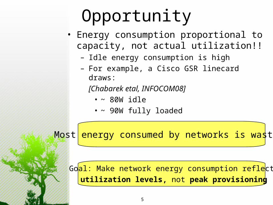
Opportunity• Energy consumption proportional to capacity, not

actual utilization!!– Idle energy consumption is high– For example, a Cisco GSR linecard draws:

[Chabarek etal, INFOCOM08]• ~ 80W idle• ~ 90W fully loaded

Most energy consumed by networks is wasted!

Goal: Make network energy consumption reflect

utilization levels, not peak provisioning

6

Idea• Key Idea: Let network equipment sleep for brief periods or slow down

when lightly loaded to save energy• Inspiration: Use of sleep and performance states in PCs, processors

• Rationale: E ~= pidle Tidle + pactive Tactive

• Assumptions: We assume support for sleep/performance states in NICs, linecards, switches, and routers and consider how to best use them

• Depend on: – Type/extent of hardware support for sleep and performance states– Careful use of these states to protect performance and maximize savings

Sleeping reducesidle energy

Slowing downreduces both

7

Outline

1.Key questions and method2.Sleeping3.Rate adaptation (slowing down)4.Sleep vs. Rate adaptation

8

1. Key questions and method

• How much energy can we save without compromising performance?

• Can we realize these savings with practical schemes?

Methodology:1. Model hardware support for sleep and rate adaptation2. Evaluate savings/performance with simulations (ns)

• Abilene and Intel topologies and their traffic workloads

3. Look for (unrealistic) bounds as well as practical schemes

9

Model• Single sleep state with power psleep<< pidle

• δ: transition period (ms)• Timer or activity-driven wakeup• Interfaces sleep independently

Metrics• Energy savings in % time asleep • Performance in loss and max delay

2. Sleeping states

time

power

pidle

psleep

δ

(sleep)

(idle)

10

Packets over a link:

• sleep time depends on:

Buffer and burst:

When can a link sleep?

time

δ Transition time

1 2 3 4 5 6 7

Periods of sleep

δδ δ δ

time

1 2 3 4 5 6 7

Sleep

11

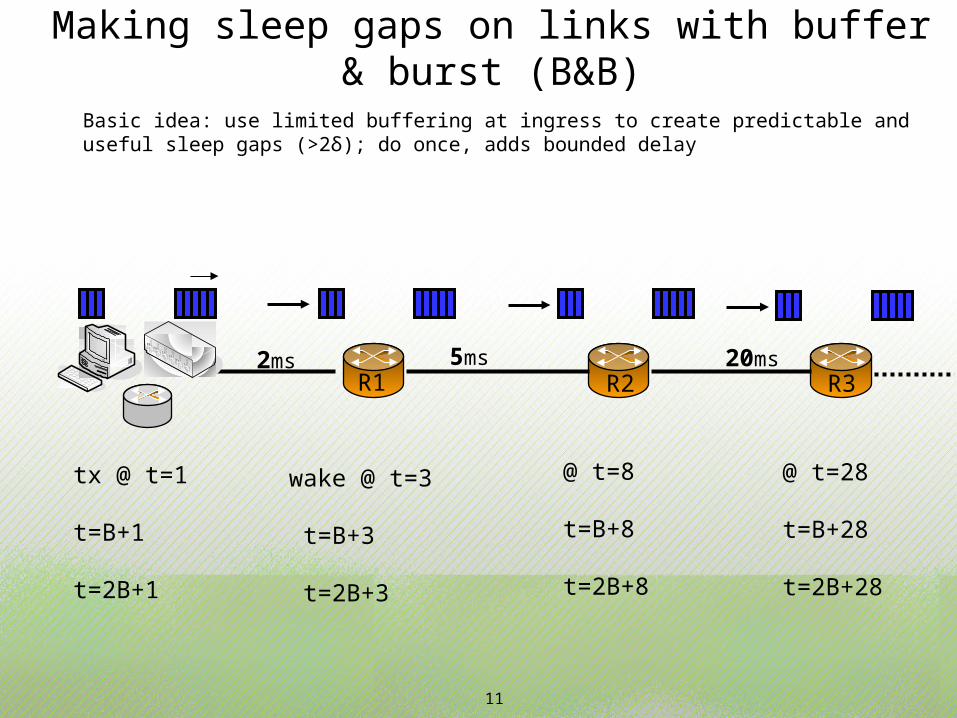
Making sleep gaps on links with buffer & burst (B&B)

Basic idea: use limited buffering at ingress to create predictable and useful sleep gaps (>2δ); do once, adds bounded delay

wake @ t=3 t=B+3 t=2B+3

` 2ms 5ms 20ms

tx @ t=1 t=B+1 t=2B+1

@ t=8 t=B+8 t=2B+8

@ t=28 t=B+28 t=2B+28

R1 R2 R3

12

Coordination among ingressesBasic idea: align bursts/gaps on links in networks by adjusting relative timing phase of different ingresses

8ms

3mst+5, t+5+B,…

t, t+B,…

coordinate burst times to align in the network

R

I1

I2

13

Potential for savings with sleep (optB&B)

• “perfect” coordination not generally possible

1ms

2ms

15ms

20ms

t1

t2

• Upper bound (optB&B): Global search to find ingress transmission times that maximize network-wide sleep

I1

I1

R1

R2

t1 + 1ms = t2 + 20ms

t1 + 15ms = t2 + 2ms

14

Potential benefits of sleeping

A little shaping can get most of the utilization gain

Abilene, transition time=1ms, B=10ms

Upper bound withoutbuffering/shaping

Upper boundfor any scheme

idle (bound)WoA (pareto)WoA (CBR)optB&B(CBR)

Upper bound withbuffering/shaping

15

Practical sleeping algorithm (practB&B)

1. Ingress buffers and transmits packets in a bunch every Bms2. Within bunch, packets are organized by egress3. Router interfaces wake to process bursts4. Router interfaces sleep if start of next burst is >2δ ms away

16

No coordination (practB&B)

Practical algorithm realizes most of the benefit

Abilene, transition time=1ms, B=10ms

17

Impact of sleeping on delay

No added loss; added delay ~ bounded by Bms

Abilene, transition time=1ms98

th p

erce

ntile

del

ay (

ms)

18

Impact of sleep: Any Losses?• No additional losses are incurred until utilizations come

close to saturating some links.• Losses greater than 0.1% occur at

Scheme Utilization

Default 41%

B = 10ms 38%

B = 25ms 36%

19

Impact of sleep transition time

Quick transitions (preferably < 1ms) needed

20

Outline

1.Key questions and method2.Sleeping3.Rate adaptation (slowing down)4.Sleep vs. Rate adaptation

21

3. Rate adaptation states

Model• N performance states • Rates r1, …, rn and pi < pi+1

• δ : transition period (ms)• Interfaces can rate-adapt independently

Metrics• Energy savings in average rate reduction • Performance in loss and max delay

time

power

pi+1

pi

δ

(1G)

(100M)

22

Using performance states

Optimal algorithm: ideal service curve follows shortest Euclidean distance.

bytes arriving at router

bytes leaving router

service rate

• Basic idea: decrease rate as much as possible without introducing more than than d ms per hop

23

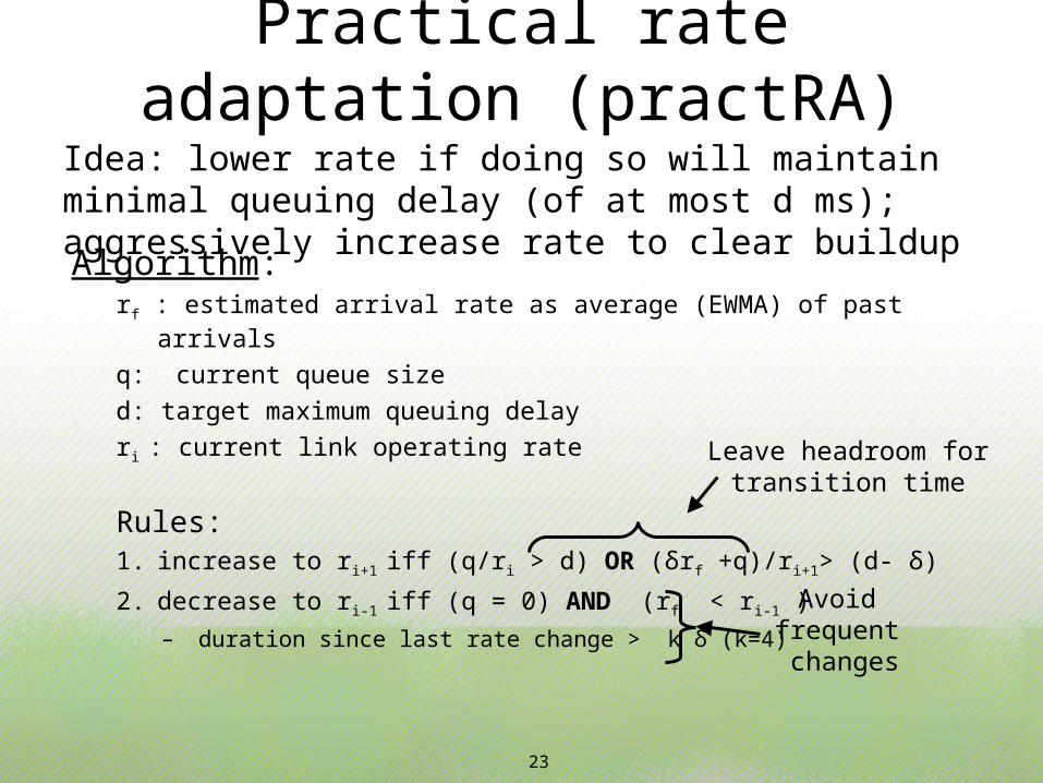
Practical rate adaptation (practRA)Idea: lower rate if doing so will maintain minimal queuing delay (of at most d ms); aggressively increase rate to clear buildup

Algorithm:rf : estimated arrival rate as average (EWMA) of past arrivals

q: current queue sized: target maximum queuing delayri : current link operating rate

Rules: 1. increase to ri+1 iff (q/ri > d) OR (δrf +q)/ri+1> (d- δ)

2. decrease to ri-1 iff (q = 0) AND (rf < ri-1 )– duration since last rate change > k δ (k=4)

Leave headroom fortransition time

Avoid frequent changes

24

Benefits of rate adaptationAbilene, transition time δ =1ms, d=3ms

Upper boundfor any scheme

Practical rate adaptation close with uniform rates

Far with exponential rates• Added delay < d * (#hops)

• No observed packet loss

25

Outline

1.Key questions and method2.Sleeping3.Rate adaptation (slowing down)4.Sleep vs. Rate adaptation

26

Models of future power profiles

pactive = C + fn(rate)

pidle = C + β fn(rate)

psleep = μ pidle(rmax)

Fraction of power that doesn’t scale with rate

Idle/Active Workload Ratio

Rate scaling function

fn(rate) ~ ratefrequency scaling

fn(rate) ~ rate3

dynamic voltage scaling

Power reduction using sleep

27

Sleeping and rate adaptation (DVS-r3)

28

Sleeping and rate adaptation (Frequency Scaling -r)

29

ObservationsThe authors say

“Hence to avoid complex interactions, we consider that the whole network , or at least well-defined components of it, run either rate adaption or sleep”

But both schemes can be combined to give better results.For eg: In rate adaptation one can try to put the links to sleep instead of keeping them in the idle state.

30

ObservationsWhen rate adaptation is done using frequency scaling the authors themselvessay that for values (C=0.3 and β =0.1) and (C=0.3 and β =0.8) the savings obtained are poor and add little additional information.

My observation is that rate adaptation (frequency scaling) gives no gain in terms of energy.

31

Thank you. Questions?