reentrant fms scheduling in loop layout with consideration ... · reentrant fms scheduling in loop...

ORIGINAL ARTICLE

Reentrant FMS scheduling in loop layout with considerationof multi loading-unloading stations and shortcuts

Achmad P. Rifai1 & Siti Zawiah Md Dawal1 & Aliq Zuhdi1 &

Hideki Aoyama2 & K. Case3

Received: 31 August 2014 /Accepted: 5 June 2015# Springer-Verlag London 2015

Abstract The scheduling problem in flexible manufacturingsystems (FMS) environment with loop layout configurationhas been shown to be a NP-hard problem. Moreover, the im-provement and modification of the loop layout add to thedifficulties in the production planning stage. The introductionof multi loading-unloading points and turntable shortcut re-sulted on more possible routes, thus increasing the complex-ity. This research addressed the reentrant FMS schedulingproblem where jobs are allowed to reenter the system andrevisit particular machines. The problem is to determine theoptimal sequence of the jobs as well as the routing options. Amodified genetic algorithm (GA) was proposed to generatethe feasible solutions. The crowding distance-based substitu-tion was incorporated to maintain the diversity of the popula-tion. A set of test was applied to compare the performance ofthe proposed approach with other methods. Further computa-tional experiments were conducted to assess the significanceof multi loading-unloading and shortcuts in reducing themakespan, mean flow time, and tardiness. The resultshighlighted that the proposed model was robust and effectivein the scheduling problem for both small and large sizeproblems.

Keyword Reentrant FMS scheduling .Multiloading-unloading and shortcuts . Genetic algorithm .

Crowding distance-based substitution

1 Introduction

FMS are important systems to satisfy the flexibility and pro-ductivity needs ofmanufacturing enterprises. A FMS typicallyconsists of CNC machines with automated tool magazines,material handling systems, and computer workstations, con-nected together mechanically and controlled by a computercontrol system. Operation management in FMS is an intracta-ble task for engineers as well as technical manager due to thecomplexity of the systems. Therefore, to manage the FMSeffectively, more performance-related decision-making is im-plemented when compared to conventional manufacturingsystems, which use a transfer line or job shop productionsystem [1].

FMS covers a wide variety of automated manufacturingsystems. A loop layout, consisting of several machines con-nected by a material handling system in circular form, is oneof the most commonly used configurations in FMS. Materialflows and part routes in FMS using loop layouts are morecomplex than the in-line layout. Due to its cyclical nature,the machine visiting sequence of a part is different from itsoperation sequence, depending on the machine arrangement.Previous studies have concerned about the improvement inloop layout configurations. Recently, the addition of multiloading-unloading (L/U) stations and shortcuts greatly im-proves the performance of loop layout configurations withsignificant decreases in the traveling distance [2, 3]. However,the improvements increase the complexity of the loop layoutsystem. As a result, improvements in production planning andcontrol are also required. Scheduling, considered as the heart

* Achmad P. [email protected]

Siti Zawiah Md [email protected]

1 Department of Mechanical Engineering, Faculty of Engineering,University of Malaya, 50603 Kuala Lumpur, Malaysia

2 School of Integrated Design Engineering, Keio University,Tokyo, Japan

3 Mechanical and Manufacturing Engineering, LoughboroughUniversity, Loughborough, Leicestershire, UK

Int J Adv Manuf TechnolDOI 10.1007/s00170-015-7395-5

http://crossmark.crossref.org/dialog/?doi=10.1007/s00170-015-7395-5&domain=pdf

of production planning and control, is also affected and needsto be updated.

The scheduling problem of FMS is known to be a NP-hardproblem where the increase of problem size causes the timesto solve the optimization problem to escalate exponentially.Moreover, production planning and control in FMS are moredifficult than those of mass production systems [4]. FMS canprocess different parts while using the same configuration ofmachines where each machine in FMS can perform variousoperations. The combinatorial characteristic of the assign-ments and tasks sequencing decisions encountered is thesource of complexity of scheduling in FMS. In addition,FMS scheduling also takes into account the technological,capacity, and availability constraints as the limiting resources,such as machines, buffers, tools, and material handling de-vices [5].

Studies on the scheduling aspect are required to catch upwith the improvement in the design sector. Since most previ-ous research addressed the scheduling problem for simpleloop layout based FMS, improved scheduling models areneeded to accommodate the addition and modification in looplayout based FMS. The improvements in layout design in-crease the complexity of the scheduling problems. Hence,improvement in the optimization method is essential to solvethe scheduling problem effectively and efficiently. This re-search deals with the reentrant FMS scheduling problem withconsideration of the improvements in the loop layout design.In particular, the scheduling model for accommodating theissues in addition of multi L/U stations and turntable shortcutin loop layout configurations is considered as the main contri-bution. A modified GA is proposed to determine near optimalsolutions within acceptable solution times. The approach em-ploys a substitution based on crowding distance to replace theindividuals with close proximity. The use of meta-heuristictechniques is necessary since the FMS scheduling problemismore complicated than scheduling in a conventional system.Furthermore, discrete event simulation based modeling is de-veloped to verify the outcome of the model. The simulation isused to validate and evaluate the part schedule and routingoptions generated by the modified GA approach.

The rest of the article is organized as follows. Section 2provides a brief literature review of FMS scheduling. Section 3presents the definition and formulation of the scheduling prob-lem in loop layout based FMS. Section 4 explains the pro-posed approach. In Sect. 5, numerical results and simulationexperiments are reported and discussed. Finally, conclusionsare outlined in Sect. 6.

2 Literature review

FMS scheduling has been an active research area because ofits importance in the today’s manufacturing industry. Due to a

high degree of product variability in FMS, the part routing andpart flows are of considerable concern. There are two opera-tional policy in the FMS scheduling. The first is the toolmovement policy where parts are assigned to machines andnecessary tools are brought to the machines to finish the op-erations. The second option is part movement policy whereparts are transferred from one machine to the others based onthe operation process. Part movement policy is implementedin most manufacturing systems because it has the advantageof ensuring that all parts can be processed using the capabili-ties of the machines. Besides that, there has been research ofother scheduling problems such as that by Hall et al. [4] whichconsidered the material handling scheduling. Some studieshave also attempted to integrate part scheduling with tool se-lection and/or material handling scheduling like the study byGamila andMotavalli [5] and Zeballos et al. [6]. Nevertheless,the majority of the research considered the part movementpolicy as the main concern.

Based on the types of FMS, a classification system wasproposed byMacCarthy and Liu [7], consisting of single flex-ible machine (SFM), flexible manufacturing cell (FMC),multi-machine flexible manufacturing system (MMFMS),multi-cell flexible manufacturing system (MCFMS), and un-specified system. The simple loop layout can be classified asFMC. However, the modified loop layout configuration canfall intoMMFMS and/orMCFMS dependent on the complex-ity. The studies by Haq et al. [8] and Keung et al. [9] areexamples of research which have addressed FMC scheduling.Due to the growth of complexity, MCFMS has been exten-sively highlighted in recent years. The studies by Das andCanel [10], Sankar et al. [11], and Jerald et al. [12] are exam-ples of research that took into account MCFMS configuration.

The cyclic scheduling problems have been reviewed,mostly in the form of reentrant flow shop scheduling prob-lem (RFSP). Huang et al. [13] addressed the reentrant two-stage multiprocessor flow shop scheduling with due win-dows. The same problem was also concerned by Jeong andKim [14] while considering the sequence-dependent setuptimes. However, the reentrant scheduling has not beenwidely addressed in FMS problems. In contrast to RFSP,different operation sequences of jobs are given in the reen-trant FMS scheduling problem. Das and Canel [10] consid-ered the scheduling problem in MCFMS with standard loopand sequential configuration which used the fixed type au-tomated handling such as belt conveyors, tow lines, androller conveyors. The study focused on the higher-levelbatch scheduling which was the sequence of batches to beprocessed in the machine cell. The FMS configuration ad-dressed by Burnwal and Deb [15] consists of several FMCserviced by AGV to transport the parts between FMCs. Theconfiguration used a single loading/unloading points andan automated storage/retrieval system to store work inprogress. Souier et al. [16] also employed single loading/

Int J Adv Manuf Technol

unloading points with one AGV to transport the parts be-tween machines.

The previous studies did not necessarily highlight the sameproblems as they differed in the type of FMS, schedulingproblems, scheduling type and the objective functions used.Joseph and Sridharan [17] evaluated the effect of dynamicdue-date assignment models, routing flexibility levels, se-quencing flexibility levels and part sequencing rules on theperformance of FMS in standard loop configurations. Thestudy proposed the development of a model called dynamical-ly estimated flow allowance (DEFA). Cardin et al. [18] pre-sented the group scheduling method using an emulation of acomplex FMS with loop configuration. The study focused ondetermining the ability of the group scheduling in absorbinguncertainties in complex FMS. Udhayakumar and Kumanan[19] addressed the integration between production scheduleand material handling schedule for a U Loop layout in theFMS. In the first phase, the FMS production schedule, withminimizing makespan as the objective function, was generat-ed using the Giffler and Thompson algorithm. Then, the out-put of production scheduling was used to develop materialhandling schedules.

Hsu et al. [20] attempted tominimize the work in process tosatisfy economic constraints. A two-step resolution approachwas presented to solve the problem. Petri net modelling of theproduction process was applied for constructing the model ofthe problem. Afterward, a genetic algorithm was used to ob-tain the sequence of tasks for a flexible manufacturing cell. Inaddition to the static environment, dynamic scheduling hasbeen developed as an alternative approach to mimic real-lifedynamic environments. Qin et al. [21] examined dynamicscheduling for an interbay automated material handling sys-tem configuration. The configuration was a single loop, spinetype interbay material handling route. The AGVs movedaround the path in unidirectional movement. Alternativeshortcut paths were placed to connect the upper and lowerrows of the main loop. A genetic programming based CDRgenerator was proposed to generate the composingdispatching rule that can be used in real-life dynamic produc-tion. The dispatching of AGV in the FMS was also concernedby Caridá et al. [22] in which the factory layout was modeledin Petri nets.

Objective functions hold the central role for optimization inFMS scheduling problems. Several measurements have beenused as the indicators of system performance. Minimizingmakespan is the most common objective function, as indicat-ed by researchers in the FMS scheduling problems [23–27].Other research has tried to use other approaches, i.e. reducingwork in process [20, 28]. However, in practical applications,there are many objectives that have been considered in sched-uling problems. This has indicated that evaluating a singleobjective is not satisfactory for improving the performanceof the complete manufacturing systems [29]. In addition,

satisfying a single objective cannot resolve the trade-off be-tween criteria. Therefore, it is important to consider multipleobjective functions simultaneously since a greater variety ofperformance indicators can be accommodated. Joseph andSridharan [17] employed mean flow time, mean tardiness,percentage of tardy parts and mean flow allowance. Prakashet al. [30] utilized bi-objective functions which are mean flowtime and throughput to quantify performance. Jerald et al. [12]aimed to minimize idle time and the penalty cost for not meet-ing delivery dates by proposing simultaneous scheduling ofparts and AGV. Ebrahimi et al. [31] used the combination ofminimizing makespan and tardiness. These criteria representthe two important issues in the industries, the maximizingproductivity of line production and fulfilling the customerexpectation.

Related to the methods used, there are two categories ofapproach: optimization methods for exact solutions usingmathematical programming and meta-heuristic algorithmsfor near optimal solutions. An example of the use of mathe-matical programming methods is the branch and bound solu-tion method proposed by Das and Canel [10] to exploit thespecial structure of the problem in developing strong lowerbounds. The problem was modeled for a MCFMS withflowshop characteristics. A MCFMS consists of a number offlexible manufacturing cells, and possibly a number of singleflexible machines, connected by an automated material han-dling system. Minimizing makespan was set as the objectivefunction.

In recent research, meta-heuristic became the trend of re-lated studies since they possess the learning ability, which thetraditional scheduling techniques do not have [32]. Somemeta-heuristics have been shown to provide good perfor-mance solutions in previous studies. Low et al. [33] proposedthe combination of Simulated Annealing (SA) and TabuSearch (TS). The hybrid heuristic was used to solve the ad-dressed FMS scheduling problem with three performance in-dicators, mean flow time, mean machine idle time, and meanjob tardiness, simultaneously. Two heuristic procedures fromtheir previous work [34] called sequence-improving proce-dure (SIP) and routing-exchange procedure (REP) were im-plemented using SA and TS. As a result four different hybridsearching structures were generated, depending on whichsearching procedure was adopted in REP and SIP, respective-ly. Baruwa and Piera presented timed colored Petri nets, com-bining evaluation methods (simulation) and search methods(optimization) [35]. The proposed approach was aimed to findthe near optimal solutions in short computation time. Othermethods commonly used in the scheduling problems belongto Swarm intelligence family, including ant colony optimiza-tion [36], pheromone approach [37] and chemotaxis-enhancedbacterial foraging algorithm [38].

Genetic algorithms are the most popular meta-heuristictechniques used in FMS scheduling problems. Kim et al.


[39] developed a network-based hybrid GA. The proposedmethod was combined with the neighborhood search tech-nique in a mutation operation to improve the solution of theFMS problem and to enhance the performance of the geneticsearch process. Prakash et al. [30] developed a novel approachcalled a knowledge based genetic algorithm (KBGA) by com-bining GAwith knowledge management. Godinho Filho et al.[40] reviewed the use of genetic algorithms to solve schedul-ing problems in FMS. There were four conclusions from thisliterature study: (i) there was a switch of direction where meta-heuristics, especially GA and its hybrid have become popular(ii) although most studies dealt with complex environmentsconcerning both the routing flexibility and the job complexity,only a minority of papers simultaneously considered the vari-ety of possible capacity constraints on an FMS environment(iii) local optimization methods were rarely used; (iv)makespan was the most widely used measurement of perfor-mance. In summary, the GA has proven successful when im-plemented in various FMS scheduling problems. Thus, it isworth developing a modified GA for further study.

From the point of view of layout system complexity, pre-vious studies considered relatively simple configuration.Meanwhile, the loop layout configuration has recently beenextensively modified to increase its performance and flexibil-ity. Some examples of improvement in the loop layout designare the addition of turntable shortcuts [2] and multi loading-unloading points [3]. Since these additions have not previous-ly been included, more studies are required to cover the gap inthe complex loop layout system. Thus, based on the literaturereview and our best knowledge, this study emphasizes thedevelopment of a part scheduling model for complex looplayout in FMS. The model accommodates the addition ofmulti loading-unloading points and turntable shortcut in theconfiguration. A modified GAwith crowding distance basedsubstitution is proposed to solve the reentrant FMS schedulingproblem.

3 Problem formulation

3.1 Reentrant FMS scheduling

Loop layout consists of several machines connected by mate-rial handling in a circular form. The reentrant characteristicallows the part to reenter the system and revisit particularparts, thus forming cyclic traveling routes. In this study, theterm of job and part are interchangeable, in which both indi-cate the same meaning. Scheduling in FMS can be consideredas the combination of flowshop and jobshop scheduling withadditional constraints. Figure 1 illustrates the example config-uration of the modified loop layout.

An example taken from previous literature [19] with addi-tional properties is presented to illustrate the scheduling

problem in loop layout FMS. There are four parts to be proc-essed in seven different machines with distinct due dates. Inparticular operations, there are alternative machines which canbe used to substitute the main machine. Thus, there are manypossible routing options for the parts. The number of possibleprocessing sequence depends on the alternative machines,which can be calculated as 2n, where n is the number of alter-native machines corresponding to each part. Table 1 shows anexample of operation sequence.

In the example, the number of alternative machines n=3that can be used to process part 1, thus there are 23=8 possibleprocessing sequence. The parts are allowed to enter and exitfrom the system which results in minimum travel distance.The parts enter using the nearest loading point prior to themachine used to process the first operation, and exit fromthe nearest unloading point subsequent to the machine usedto process the last operation. The model is also built based onthe assumption that whenever circumstances are possible, ashortcut is always used to minimize the travel distance.

This study addresses the determination of two criteria inproduction planning, the part dispatching schedule androuting choice. The dispatching schedule is a permutationvariable that indicates the dispatching sequence of the parts.Since this study covers the multi loading and unloading pointaddition, the permutation characteristic is exclusively applied

Buffer 7

Buffer 6

Buffer 5

Buffer4

Buffer 2Buffer 1

Buffer 3

M2 M6 M3

M1

M5 M4 M7

Loading

Unload Shortcut

Loading

Unloading

Fig. 1 Example of modified loop layout configuration

Table 1 Example of operation sequence matrix

Part types Operation sequence Due date

1 2 3 4

Part 1 M1 M4 M2 M7 200

M3 – M6 M5

Part 2 M1 M6 M3 M4 180

M2 M5 – M7

Part 3 M2 M6 M3 M5 140

M1 M4 – –

Part 4 M3 M4 M2 M7 190

M6 M5 – M1


for the parts at the same loading point. Unlike in conventionalmanufacturing systems, FMS allows the parts to be processedby alternative machines for particular operations. This condi-tion results in the various routing options for the parts. Therouting choice not only determines the machine visiting se-quence, but also the processing time and setup time for eachoperation that will affect the completion time of the parts.Thus, the proposedmodel considers the routing choice of eachpart to get the most optimized schedule.

3.2 Mathematical model

The FMS considered consists of a set of machines J, which arearranged in a cyclic layout connected with a conveyor. Thereare several shortcuts inside in particular positions. The mainconveyor of the loop is unidirectional, while the shortcuts’conveyor is bidirectional. Beside the main loading-unloadingpoint, there are extra loading-unloading points placed insidethe loop. These points can either contain only loading orunloading points or can also contain both loading-unloadingpoints. The parts can enter the system using any loading point land leave the system as a product from any unloading point u.

There is a set of parts K that must be processed. A set ofoperations I corresponding to part k is processed by specificmachine j. Every process follows the job sequence of each partdenoted by Sk. This means that an operation ikt of part k cannotbe processed before the predecessor operation ikt−1 has beencompleted. The transport time is denoted by τ, which dependson distance to be traveled by the part to perform operation iafter completion of operation i−1, denoted by d. In the case oftransport time in shortcuts and from/to loading-unloadingpoints, the same symbol is applied. Table 2 lists the notationsuse in the mathematical model.

The machines can only process one part at the same time.The parts will be placed in the buffer which is positioned justbefore the machine if there is another part being processed bythat machine. The duration between the parts entering thebuffer until the part enters the machine is described as delayd. The manufacturing process of part k in machine j will takesome time expressed by the processing timeφijk. In FMS, eachmachine can perform various operations for different parts.However, a particular time is needed to setup the machinebefore processing a different type of parts. This is denotedby the setup time εijkwhich corresponds to part k and machinej.1.

Multi-objective functions, consisting of minimizingmakespan Cmax, mean flow time Tf and tardiness Tt, wereused as the approach to measuring production efficiency andresource utilization. The objective functions also represent theinterest in the real problem faced by the manufacturing indus-tries [20].

Objective functions:Minimize

Cmax ¼ maxi; j;k

Ci jk

� � ð1Þ

T f ¼ 1

P

XP

k¼1

maxi; j

Ci jk

� � ð2Þ

Tt ¼XP

k¼1

max maxi; j

Ci jk

� �−tdk ; 0

� �ð3Þ

Equations 1, 2, and 3 describe the objective functions,which are makespan, mean flow time, and total tardiness,respectively. Cijk is the integer value of the completion timeof operation i onmachine j for each part k. tdk is the due date ofpart k. The total fitness is the sum of each objective function

Table 2 Lists of notations

Index Description Index DescriptionSubscripts Parameters

k Part to be processed τj Transport time

i Operations of the parts to be machined φijk Processing time of operation i of part k in machine j

j Machines that carry out the operations εijk Setup time of operation i of part k in machine j

u Loading point Cijk Completion time of operation i on machine j for part k

l Unloading point Stijk Starting time of operation i on machine j for part k

h Turntable shortcut tdk Due date of part k

Sets t Time

K Set of parts αijk Decision variable which has the value 1 if the operation iof part k is assigned to machine j, 0 otherwise

I Set of operations μku Decision variable which has the value 1 if part k is loadedusing loading point u, 0 otherwise

J Set of machines λkl Decision variable which has the value 1 if part k is unloadedusing unloading point l, 0 otherwise

Sk Set of operations sequence of part k


with equal weighting factor. Thus, each objective function hasequal significance. The objective functions are subject to thefollowing constraint.

XMJ

αi jk ¼ 1; ∀i; k ð4Þ

Ci jk ≥C i−1½ � jk þ ϕi jk þ τ ii0

þ εi jk ; i ¼ 2; 3;…Ik ∀ j; k ð5Þ

τ ii0 ¼XMj¼1

XMj0 ¼1

XI

i0¼1

d j j0 ⋅αi jk ⋅αi0 j0k 0 ∀i; k ð6Þ

Ci jk ≥0 ; ∀i; j; k ð7ÞSti jk ≥0 ; ∀i; j; k ð8ÞXUu

μku ¼ 1 ; ∀k ð9Þ

XL

l

λkl ¼ 1 ; ∀k ð10Þ

Sti jk ≥C i−1ð Þ jk þ τ j0 ∀ j; k ð11Þ

Equation 4 states that one machine must be selected foreach operation. αijk is a decision variable which will havethe value 1 if the ith operation of part k is assigned to machinej, and 0 otherwise. Equation 5 ensures that the completiontime of operation i on machine j for part k, must be greaterthan the predecessor operation i−1, by at least the processingtime required for an operation i plus transport time and setuptime for operation i of part k on machine j. Equation 6 definesthe transport time which is calculated by the distance betweenmachine j used to process operation i and machine j’ used toprocess operation i’.

Equation 7 defines that each operation begins after timezero. Equation 8 describes the nonzero property of completiontime operation i of part k. Equations 9 and 10 ensure that theparts can only be loaded and unloaded by one loading and oneunloading station. Note that μku=1 if part k is loaded by load-ing u. Similarly, λkl=1 if part k is unloaded using unloading l,0 otherwise. Equation 11 ensures that the starting time ofoperation i of part k must not be earlier than the sum of com-pletion time of the predecessor operation i−1 of the same joband the transport time.

4 Proposed approach

In solving the scheduling and assignment problems ofFMS, past studies have adopted mathematical program-ming techniques. However, in real-world problem in-stances, it has been seen that the traditional techniques

cannot reach optimal solutions [17]. Thus, the use ofmeta-heuristic optimization, also known as artificial intel-ligence techniques, has been considered. This study ad-dresses the use of a modified genetic algorithm to solvethe scheduling problem. The GA aims to seek the optimumvalue of objective function f which is influenced by a vec-tor of decision variables x. Each individual represents apotential solution to the problem at hand. Then, the indi-vidual is evaluated to give some measures of its fitness.Some individuals experience stochastic transformation bymeans of genetic operations to form new individuals.There are two types of transformation: crossover, whichcreates new individuals by combining parts from two par-ent individuals, and mutation, creating new individuals bymaking changes in a single chromosome.

One of the keys to good performance in GAs is main-taining the diversity where it should be prominent in anyapplication [41]. In the GA, the nature of crossover leads topremature convergence since it tends to produce uniformoffspring. Moreover, the implementation of roulette wheelselection allows the good individuals to be selected repeat-edly. This condition results in difficulty in maintaining thepopulation diversity. As a solution, the modified GA incor-porates the crowding distance to evaluate the similaritybetween individuals. Individuals’ substitution engagingthe elitist based re-combination and re-mutation method isused to produce the substitute. The scheme of the proposedapproach is illustrated in Fig. 2.

After several generations, the algorithm converges to thebest individual, which represents an optimal solution. The GAparameters in the proposed approach are set as follows: thepopulation size Ps=20, crossover rate Pc=0.8, and mutationrate Pm=0.025 [12, 42]. The loop process continues until thetermination criterion is fulfilled, when the numbers of gener-ations N=100.

4.1 Coding representation

The GA process starts with coding representation. In optimi-zation problems of FMS scheduling, the main decision vari-able is the sequence of each part that will enter the system.Each part number may be considered to be a gene on chromo-some represented using integer permutation chromosomes.Since each gene represents a part number, the greater numberof parts means longer chromosomes. Table 3 depicts the inte-ger permutation chromosomes; the numbers represent the partcodes.

The chromosomes represent the two variables to be opti-mized. The first layer depicts the input part sequence. It is aninteger permutation, corresponding to the loading groups. Thesecond layer describes the selected route of each part. Eachpart may have a different number of routing options


depending on the operations, layout structure, and the alterna-tive machines that can be used to process the part.

4.2 Parent selection

The initial population of solutions is produced by utilizing astochastic technique. A set of decision variables is portrayedby coded strings of finite length. A roulette wheel is employedas the parent selection method, in which the probability of anindividual i being selected is dependent on its fitness value fias defined in Eq. 12.

pi ¼ f i.Xn¼1

i¼1

f i ð12Þ

When the inequality p0+p1+…+pi−1<γ≤p0+p1+…+pi−1+pi is met, the individual i is selected for the next gen-eration. To ensure that good chromosomes have a higher pos-sibility of being picked, ranking schemes are always adopted.This scheme is performed by sorting the population on thebasis of fitness values and then the selection operation is un-dergone based upon the rank. Therefore, individuals with highfitness values have a greater chance of being chosen asparents.

4.3 Crossover

The crossover operator used in this research is a partiallymatched crossover (PMX). The crossover operator divideseach selected individual into two or more sections and swapsthe divided sections of the individual. Figure 3 illustrates thecrossover operation involving PMX techniques.

4.4 Mutation

Since an integer permutation representation is used in thisstudy, the exchange mutation, also called swap mutation, isapplied. In this technique, two genes are picked randomly andtheir alleles get exchanged. Figure 4 shows the mutation pro-cess using swap mutation.

Unlike the crossover which operates on the individual level(swapping certain parts between two individuals), mutationoperators operates on the gen level. Therefore, the processmay result to an infeasible string where route choices maynot be available. To accommodate this issue, we perform anadjustment process for allele value which violates the con-straints, i.e., the value of selected route exceeds the numberof possible routes. The new values are randomly generatedamong all possible routes.

4.5 Crowding distance calculation

The level of population diversity can be estimated usingcrowding distance, which is an estimate of the perimeter ofthe cuboid formed by using the nearest neighbors as the ver-tices [43]. The proposed approach uses the genotype basedcrowding distance, calculated using the Euclidean distance.Since there are two variables to be optimized, the computationuses a two dimension average Euclidean distance calculation,

Start

Codingrepresentation

Selection

Crossover Mutation

Does the individualmeet the distance

threshold?

Stop

Is terminationcriteria fulfilled?

Generation of Initialpopulation

Crowding-distancecomputation

Fitness evaluation Individualssubstitution

New Population

Acquiring the bestsolution

Is the individualoriginal solution?

yes

yes

yes

no

no

no

Fig. 2 Scheme of modified GA

Table 3 Integer permutation chromosome illustration

P1 P2 P3 P4 P5 P6 P7 P8 P9 P10

Sequence 9 1 3 8 6 2 4 5 7 10

Selected route 2 3 1 4 2 4 1 3 4 5

P1 P2 P3 P4 P5 P6 P7 P8 P9 P10

Parent 19 1 3 8 6 2 4 5 7 102 3 1 4 2 4 1 3 4 5

Parent 28 3 7 4 5 6 1 10 2 93 1 4 5 3 1 4 2 5 2

Offspring 19 1 3 8 5 6 1 10 7 102 3 1 4 3 1 4 2 4 5

Offspring 28 3 7 4 6 2 4 5 2 93 1 4 5 2 4 1 3 5 2

After adjustment

Offspring 19 2 3 8 5 6 1 10 7 42 3 1 4 3 1 4 2 4 5

Offspring 28 3 7 1 6 2 4 5 10 93 1 4 5 2 4 1 3 5 2

Fig. 3 PMX crossover


presented in Eq. 13.

d p; qð Þ ¼ 1

N

XNn¼1

ffiffiffiffiffiffiffiffiffiffiffiffiffiffiffiffiffiffiffiffiffiffiffiffiffiffiffiffiffiffiffiffiffiffiffiffiffiffiffiffiffiffipnx−qnxð Þ2 pny−qny

� �2r

ð13Þ

where p is the allele value of individual i and q is the allelevalue of individual i−1. Subscript x represents the part sched-ule. Subscript y represents the routing options. The order ofallele is represented by n, where N indicates the length ofchromosomes. The distance computation requires sorting thepopulation according to objective function value in descend-ing order of magnitude. In this scheme, the elitist individualwill always be kept. Individuals which have close proximitywith the predecessor solutions will be replaced.

4.6 Individuals substitution

The distance computation results in several solutions whichdo not meet the threshold. To maintain the fixed populationsize, new generated offspring are used as substitutes from thereplaced individuals. The substitution of an individual in-volves two genetic processes, re-combination and re-muta-tion, to generate distinct solutions. Re-combination is basedon the crossover approach involving the elitist individual andthe individual to be replaced. Re-mutation is achieved bychanging an allele with a new randomly generated value.

4.7 Population replacement

Having finished the genetic operator, elitism is applied toallow the best solution to be preserved in the next genera-tion. In this scheme, the surviving best solution replaces theworst individual, which either comes from the previousiteration or as the result of the crossover and mutation op-erators. Thus, the good offspring will not be lost due topopulation replacement.

5 Results and discussion

5.1 Datasets and layout properties

The proposed approach was tested to measure perfor-mance. The test beds were taken from previous literatures[44–46, 19] with some modifications to conform the FMSenvironment. The jobs visit the machines in an operationsequence with the choice of selecting alternative machinesfor the operations. The operation sequence for each job is arandom permutation of the machines, while the processingtimes and setup times are uniformly distributed. Each jobhas a deadline, which is uniformly distributed on an inter-val determined by the expected workload of the system andother parameters. Since the datasets lack some of the pa-rameters, such as setup time and deadline, the missing datawere generated artificially. The layout properties were af-fected by the datasets used, especially the number of ma-chines, parts and operation sequence. The details of pointto point distance between machines and layout propertiesare given in Appendixes 1 and 2, respectively. Table 4shows the instances used to test the algorithms.

5.2 Improvement and robustness test

A comparative study was conducted to measure the perfor-mance of the proposed genetic algorithm optimizationmodel. The approach was contrasted with dispatching ruletechniques such as shortest processing time (SPT), longestprocessing time (LPT), earlier due date (EDD), and othermeta-heuristics, such as conventional GA and SA. Thecomparison was based on the objective functions whichare minimizing makespan, mean flow time, and total tardi-ness. The experiments were done by ten repetitions foreach method. Figure 5 presents the iteration charts of themodified GA in each dataset. The upper line represents theaverage fitness of the generation. The lower line representsthe best fitness obtained.

The iteration process indicated that in small datasets, e.g.,dataset 1, the GA quickly reached a stable state because therewas only a small solution space to be explored. Meanwhile, inlarge datasets, there were huge solution spaces with many

P1 P2 P3 P4 P5 P6 P7 P8 P9 P10Original chromosome

9 1 3 8 6 2 4 5 7 102 3 1 4 2 4 1 4 4 5

Mutated chromosome

9 5 3 8 6 2 4 1 7 102 2 1 4 2 4 1 3 4 5

Fig. 4 Mutation process using swap mutation

Table 4 Data sets and configurations for the case studies

Dataset No. of part types No. of machines Load station Unload station Machine arrangement

1 4 7 2 2 2-6-3-1-5-4-7

2 10 10 2 2 1-2-3-4-5-6-7-8-9-10

3 15 12 2 2 1-2-3-4-5-6-7-8-9-10-11-12

4 20 15 2 2 1-2-3-4-5-6-7-8-9-10-11-12-13-14-15

5 20 20 2 2 1-2-3-4-5-6-7-8-9-10-11-12-13-14-15-16-17-18-19-20


combinations of sequences and possible routing options.Thus, the searching process in large datasets took more itera-tions to converge than in small datasets. Besides comparison

of each objective function, the total fitness was alsocontrasted. The improvement rate IR of the proposed approachover method A is defined in Eq. 14.

b) Data set 2 c) Data set 3

d) Data set 4 e) Data set 5

a) Data set 1

Fig. 5 Iteration charts of the proposed method


Table 5 Value of objective functions obtained and improvements

Indicator Method Datasets

1 2 3 4 5

Makespan SPT 330 1852 1358 945 4669

LPT 382 1880 1220 962 4465

EDD 382 1773 1357 1040 4624

SA 322 1769 1248 955 4294

GA 322 1768 1308 889 4525

Modified GA 322 1727 1219 900 4147

Mean flow time SPT 265 1616 1121 722 3873

LPT 302 1648 1058 731 3810

EDD 302 1591 1122 721 3883

SA 265 1557 1056 713 3719

GA 265 1547 1030 688 3635

Modified GA 265 1493 1023 684 3622

Total tardiness SPT 349 1923 3749 5662 22,750

LPT 499 2240 2803 5848 21,381

EDD 498 1703 3756 5655 22,843

SA 350 1440 2804 5489 19,972

GA 350 1328 2519 4980 18,363

Modified GA 350 997 2366 4910 17,658

Total fitness SPT 944 5391 6228 7329 31,292

LPT 1183 5768 5081 7541 29,656

EDD 1182 5067 6235 7416 31,350

SA 937 4766 5108 7157 27,985

GA 937 4643 4857 6557 26,523

Modified GA 937 4217 4608 6494 25,427

Improvement rate IR of modified GA over SPT 0.74 % 21.78 % 26.01 % 11.39 % 18.74 %

LPT 20.79 % 26.89 % 9.31 % 13.88 % 14.26 %

EDD 20.73 % 16.78 % 26.09 % 12.43 % 18.89 %

SA 0.00 % 11.52 % 9.79 % 9.26 % 9.14 %

GA 0.00 % 9.18 % 5.13 % 0.96 % 4.13 %

Table 6 Robustness improvement ratio of modified GA, in contrast to SA and GA

Datasets SA GA Modified GA Robustness improvement ratio

Best (worst) Average (std.) Best (worst) Average (std.) Best (worst) Average (Std.) mGA vs. SA mGA vs. GA

1 937 945 937 942 937 939 96.64 % 90.54 %

964 8.02 954 4.78 940 1.47

2 4766 4992 4643 4977 4217 4402 16.42 % 60.53 %

5286 131.91 5188 191.97 4590 120.60

3 5108 5456 4857 5126 4608 4806 21.83 % 32.76 %

5637 154.99 5450 167.11 5057 137.03

4 7157 7328 6557 6822 6494 6573 43.44 % 75.18 %

7440 83.82 7008 126.53 6685 63.04

5 27,985 28,944 26,523 27,541 25,427 26,193 17.15 % 30.51 %

29,746 566.03 28,558 618.04 26,977 515.22


IR ¼ f i Að Þ− f i mGAð Þf i Að Þ � 100% ð14Þ

where fi(mGA) denotes the total fitness obtained by the pro-posed approach and fi(A) denotes the total fitness obtained byheuristics method A. Table 5 shows the best results of eachmethod and the improvements, in term of total fitness, obtain-ed by the proposed approach compared to other methods.

Based on the numerical results, the modified GAoutperformed the other methods in all case studies in terms of

overall fitness value. The results of case studies also depictedthe consistency of modified GA, either applied in small or largedatasets. To further examine the performance of modified GA,this study calculates the robustness improvement ratio in con-trast to the simple GA and SA as defined in Eqs. 15 and 16.The results of robustness test are described in Table 6.

Robustness improvement ratio in contrast to simple GA

¼ 1−σ2 mGAð Þσ2 GAð Þ � 100% ð15Þ

Data set 1 Data set 4 With substitution

Data set 2 Data set 5 Without substitution

Data set 3

Fig. 6 The crowding distance of each generation


Robustness improvement ratio in contrast to SA

¼ 1−σ2 mGAð Þσ2 SAð Þ � 100% ð16Þ

The results demonstrated a significant robustness improve-ment of modified GA relative to simple GA and SA both insmall and large data. The improvement was more prominentagainst the simple GA. GA tends to narrow its search space tosmall neighborhoods when it finds a local optima and failed toexplore better solutions in other neighborhoods. When the ex-periments were replicated, the search space of simple GAwasfocused to different neighborhoods, thus it has the lowest stan-dard deviation. In contrast to simple GA, SA has better abilityto explore wider neighborhoods. However, the fitness obtainedby SAwas lower than GA andmodified GA. Although SA hadbetter robustness than GA, it was less effective. In modifiedGA, the crowding distance based substitution gives more op-portunity to broaden the search space without discarding thecurrent neighborhoods. Therefore, the modified GAwas morestable, robust and effective than other methods.

5.3 Similarity level analysis

A similarity level analysis was carried out to measure therobustness of the proposed approach. The comparison usedthe crowding distance as an approach to determine the simi-larity level. Figure 6 presents the comparison of the crowdingdistance before and after the individual substitution in each

generation. The graphs indicate that the earlier generationshad a low similarity level. Since the initial population wasstochastically generated, the individuals have a high degreeof diversity. As the iteration process continues, the diversitylevel decreases. The crossover and roulette wheel selectioncauses individuals to move toward convergence because rou-lette wheel selection allows the individuals with good fitnessto be selected with high probability. As a result, the goodindividuals dominate the next iteration and increase the simi-larity level in that generation.

The increasing of similarity results in premature convergencesince the algorithm will fail to explore new solution space. Dueto this effect, the simple GA is prone to be caught in subopti-mum solutions. The results of experiments indicated that thesimple GA failed to obtain better solutions as observed in theTable 6. It was proved that the GA was trapped in prematureconvergence. As a solution, the proposed modified GA ap-proach was intended to solve the similarity level. The approachinvolves pairwise comparison between individuals. When a pairof individuals has a low crowding distance, the worse solutionwill be substituted with a newly generated solution.

As indicated by Table 7, the individual substitutions in-creased the average distance and reduced the similarity level.It effectively improved the population diversity in all in-stances, thus reducing the possibility of being trapped in pre-mature convergence. The trend of the improvement rate showsthat small problems have higher sensitivity to the substitutionand the large data sets are more resistant toward the change. Inthe instance with fewer parts to be processed, the modificationof a gene will significantly alter the overall fitness of the chro-mosomes. Thus, it can be stated that the number of partsaffects the improvement rate on diversity.

5.4 Significance of multi L/U and shortcuts

The performance of FMS is affected by the jobs’ operationroutes as well as the traveling routes of the parts. In case of theconfiguration discussed, the addition of extra loading-unloading and shortcuts offer the alternative of part traveling

Table 8 Improvement obtained by adding extra L/U stations and shortcut

Dataset Total fitness Improvement

Without L/Uand shortcuts

With extraL/U

Withshortcut

With extra L/Uand shortcuts

Addition ofL/U stations

Addition ofshortcut

Addition of bothL/U and shortcut

1 1040 983 995 937 5.55 % 4.40 % 9.93 %

2 5126 4894 4593 4217 4.52 % 10.39 % 17.73 %

3 4955 4826 4726 4608 2.60 % 4.62 % 7.01 %

4 8833 8173 7343 6494 7.47 % 16.87 % 26.48 %

5 29,812 29,584 27,323 25,537 0.76 % 8.35 % 14.34 %

The highlighted values (lowest total fitness and highest improvement) have been pointed out in italics

Table 7 Average Euclidian distance

Data set Euclidian distance Improvementon diversity

Without substitution With substitution

1 0.053 0.068 28.30 %

2 0.485 0.533 9.90 %

3 1.731 1.867 7.86 %

4 2.289 2.369 3.49 %

5 2.736 2.827 3.33 %


routes. This section presents the analysis of the significance ofextra loading-unloading stations and shortcut addition into theloop layout in reducing the objective functions, makespan C-max, mean flow time Tf, and tardiness Tt.

A set of computational experiments was carried out byexamining the four types of configurations, which are thesimple loop layout, the addition of extra loading-unloadingstation only, the addition of shortcut only and the addition ofboth extra loading-unloading stations and shortcut. The posi-tion of loading-unloading stations and shortcut were randomlygenerated among the feasible position with assumption thenumber of L/U stations l=1, u=1, and shortcut h=1. The

experiments were based on the same parameters to ensurethe performance stability of the proposed approach.

Table 8 tabulates the result of experiments. We found thatmulti L/U stations and shortcuts result on significant improve-ment in reducing the total objective function. The addition ofshortcut showed a more substantial effect since it exception-ally important in cutting traveling distance of reentrant parts.The shortcut increases the number of possible routes to beoptimized, thus providing opportunities to generate theshortest feasible routes. The addition of L/U stations had mod-erate improvement in that the effect is limited to particularparts which belong to the extra L/U stations. However, itshould be underlined that the position of each material han-dling held important effect to the effectiveness. Therefore, thepositioning of extra L/U and shortcuts in design study is verycritical.

5.5 Simulation test

Discrete event simulation models using FlexSim softwarewere constructed to evaluate the part dispatching sequencegenerated by the proposed approach. As in the numericalstudy, three performance indicators were employed to validatethe results of the proposed method, namely flow time, tardi-ness, and makespan. The result of flow time and makespancan be acquired directly from the FlexSim simulation report.However, since tardiness is a derivation of flow time, it wascalculated as the deviation between due date and acquiredflow time. The results of both methods were compared tosee the difference between them.

The main input for the simulation study was the scheduleobtained by the proposed GA model, consisting of the arrival

Fig. 7 Simulation model in FlexSim

Table 9 Parameters of simulation model

Parameter Value

Loop conveyor length 91 m

Shortcut conveyor length 8 m

Conveyor speed 1 m/s

Distance machine to machine(start from machine 1)

3-4-4-3-3-5-5-4-6-5-4-5-6-4-5-3-4-4-4-3

Distance of load point 1 tonext machine

5 m

Distance of load point 2 tonext machine

2 m

Distance of unload point 1from previous machine

3 m

Distance of unload point 2from previous machine

2 m

Buffer capacity Unlimited

Machine capacity 1

Part schedule (obtained fromnumerical study)

Load point 1: 7-11-14-16-17-18Load point 2: 1-2-3-4-5-6-8-9-10-12-13-15-19-20


sequence and routing options of the parts. To compare theresults of both methods, the simulation model study used thesame parameter as used in the numerical study. The overallsystem was set to the same conditions as the numerical study,both on data sets (sequence, processing, and setup time) andlayout properties (machine arrangement and travel distance).Table 9 summarizes the parameters of the simulation model.

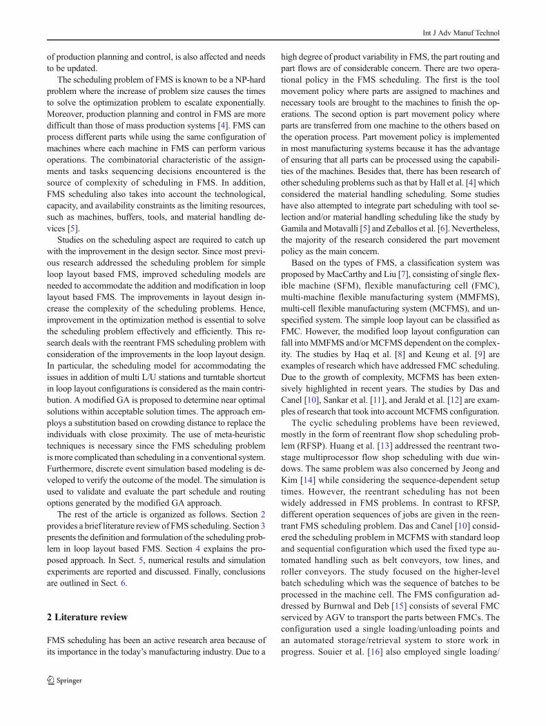
An experimental example of the simulation study involveddata set 5 since it is the most complex system in this study. Themain element of this model was the loop conveyor, construct-ed using MergeSort in FlexSim. The shortcut was representedby two conveyors with opposite movement directions. Thepick and drop points were placed along the MergeSort andconnected to queues and machines, as well as loading andunloading points. The capacity of queue was assumed to beunlimited. Meanwhile, the machines have single capacitymeaning they can only process one part at a time. Figure 7illustrates the example of simulation models on FlexSim. Theresults of the simulation experiment in FlexSim are presentedin Table 10.

Compared to the results of numerical study, there is a slightdifference between both results. Generally, the value of thesimulation result was somewhat lower than the numericalstudy result due to the different policy regarding the position-ing of pick and drop points. In the numerical study, it wasassumed that both pick and drop point of each machine werepositioned at the same point. Meanwhile, in the simulationstudy, there was a space between pick and drop points along

the conveyor. Nevertheless, the comparison indicated thatboth results are similar as depicted in Table 11.

6 Conclusion

Effective and reliable model is critical for solving the re-entrant scheduling problems in FMS with consideration ofthe addition of multi loading-unloading points and turnta-ble shortcut into the loop layout configuration. As a solu-tion, a modified genetic algorithm was developed to gen-erate the near optimal solution. The crowding factor calcu-lated using the Euclidian distance was employed to mea-sure the population diversity of the generations. Substitu-tion based on the re-combination and re-mutation was per-formed to modify the individuals with close similarity. Acomparison study between the proposed approach and oth-er conventional methods showed that the proposed ap-proach exhibited better performance and robustness thanconventional methods for both small and large datasets.The similarity analysis demonstrated that the proposed al-gorithm can tackle the population diversity issue by im-proving the crowding distance. Thus, the probability ofobtaining near optimal solutions increases by avoiding ear-ly convergence.

Although increasing the complexity, the addition alsooffers alternative routes which can be shorter in distancethan the current. The results of experiments with differentdesigns indicated that the addition L/U stations and short-cut has significant effect in reducing the makespan, meanflow time, and total tardiness by cutting the traveling timeof jobs. The outcomes of simulation confirmed that bothstudies were running alike and there were no errors in thenumerical study computation. In future studies, it is worthconsidering the other variables to develop integrated FMSscheduling by combining the parts scheduling and vehicle

Table 11 Comparison of obtained objective functions value

Objective function Numerical Simulation Difference

Makespan 4252 4174 1.83 %

Mean flow time 3688 3686 0.05 %

Total tardiness 19,037 19,040 0.02 %

Table 10 Comparison of the result of simulation and numerical study

Part Simulation result Numerical result Part Simulation result Numerical result

Flow time Tardiness Flow time Tardiness Flow time Tardiness Flow time Tardiness

1 2944 120 2967 143 11 3706 1336 3618 1248

2 3704 1457 3717 1470 12 4161 1578 4249 1666

3 3778 642 3834 698 13 4125 1976 4219 2070

4 3781 910 3372 501 14 3342 1033 3479 1170

5 4056 1855 4086 1885 15 3770 1026 3694 950

6 4174 788 4252 866 16 3634 1467 3890 1723

7 3898 1123 3911 1136 17 3062 – 3095 –

8 3145 3 3146 4 18 3930 1314 3770 1154

9 3654 313 3593 252 19 3489 647 3491 649

10 4108 1401 4109 1402 20 3266 50 3266 50


routing as well as tool selection-allocation problems toconstitute a complete scheduling system. It would also beinteresting to investigate the relationship between the im-provement in productivity and investment cost of extraL/U stations and shortcut.

Acknowledgments The authors would like to acknowledge the JapanInternational Cooperation Agency (JICA) project of the ASEAN Univer-sity Network/the Southeast Asia Engineering Education DevelopmentNetwork (AUN/Seed-Net) and the Ministry of Higher Education for fi-nancial support under High Impact Research Grant UM.C/HIR/MOHE/ENG/35 (D000035-16001).

Appendices

Appendix 1 Point to point distance

Table 12 Point to point distancein case study 1 Stations L/U point M2 M6 M3 M1 M5 M4 M7

L/U point – 3 7 11 16 20 24 27

Shortcut 1 27 30 2 6 11 15 19 22

Shortcut 2 6 9 13 17 22 26 30 1

M2 29 – 4 8 13 17 21 24

M6 25 28 – 4 9 13 17 20

M3 21 24 28 – 5 9 13 16

M1 16 19 23 27 – 4 8 11

M5 12 15 19 23 28 – 4 7

M4 8 11 15 19 24 28 – 3

M7 5 8 12 16 21 25 29 –

Table 13 Point to point distancein case study 2 Stations M1 M2 M3 M4 M5 M6 M7 M8 M9 M10

Central L/U 5 8 12 16 19 22 27 32 36 42

Extra load 40 43 2 6 9 12 17 22 26 32

Extra unload 16 19 23 27 30 33 38 43 2 8

Shortcut 1 36 39 43 2 5 8 13 18 22 28

Shortcut 2 21 24 28 32 35 38 43 3 7 13

M1 – 3 7 11 14 17 22 27 31 37

M2 42 – 4 8 11 14 19 24 28 34

M3 38 41 – 4 7 10 15 20 24 30

M4 34 37 41 – 3 6 11 16 20 26

M5 31 34 38 42 – 3 8 13 17 23

M6 28 31 35 39 42 – 5 10 14 20

M7 23 26 30 34 37 40 – 5 9 15

M8 18 21 25 29 32 35 40 – 4 10

M9 14 17 21 25 28 31 36 41 – 6

M10 8 11 15 19 22 25 30 35 39 –


Table 14 Point to point distancein case study 3 Stations M1 M2 M3 M4 M5 M6 M7 M8 M9 M10 M11 M12

Central L/U 5 8 12 16 19 22 27 32 36 42 47 51

Extra load 49 52 2 6 9 12 17 22 26 32 37 41

Extra unload 14 17 21 25 28 31 36 41 45 51 2 6

Shortcut 1 36 39 43 2 5 8 13 18 22 28 33 37

Shortcut 2 20 23 27 31 34 37 42 47 51 3 8 12

M1 – 3 7 11 14 17 22 27 31 37 42 46

M2 51 – 4 8 11 14 19 24 28 34 39 43

M3 47 50 – 4 7 10 15 20 24 30 35 39

M4 43 46 50 – 3 6 11 16 20 26 31 35

M5 40 43 47 51 – 3 8 13 17 23 28 32

M6 37 40 44 48 51 – 5 10 14 20 25 29

M7 32 35 39 43 46 49 – 5 9 15 20 24

M8 27 30 34 38 41 44 49 – 4 10 15 19

M9 23 26 30 34 37 40 45 50 – 6 11 15

M10 17 20 24 28 31 34 39 44 48 – 5 9

M11 12 15 19 23 26 29 34 39 43 49 – 4

M12 8 11 15 19 22 25 30 35 39 45 50 –

Table 15 Point to point distance in case study 4

Stations M1 M2 M3 M4 M5 M6 M7 M8 M9 M10 M11 M12 M13 M14 M15

Central L/U 5 13 20 27 36 43 50 57 64 66 72 78 86 92 98

Extra load 74 82 89 96 3 10 17 24 31 33 39 45 53 59 65

Extra unload 25 33 40 47 56 63 70 77 84 86 92 98 4 10 16

Shortcut 1 84 92 99 4 13 20 27 34 41 43 49 55 63 69 75

Shortcut 2 25 33 40 47 56 63 70 77 84 86 92 98 4 10 16

M1 – 8 15 22 31 38 45 52 59 61 67 73 81 87 93

M2 94 – 7 14 23 30 37 44 51 53 59 65 73 79 85

M3 87 95 – 7 16 23 30 37 44 46 52 58 66 72 78

M4 80 88 95 – 9 16 23 30 37 39 45 51 59 65 71

M5 71 79 86 93 – 7 14 21 28 30 36 42 50 56 62

M6 64 72 79 86 95 – 7 14 21 23 29 35 43 49 55

M7 57 65 72 79 88 95 – 7 14 16 22 28 36 42 48

M8 50 58 65 72 81 88 95 – 7 9 15 21 29 35 41

M9 43 51 58 65 74 81 88 95 – 2 8 14 22 28 34

M10 41 49 56 63 72 79 86 93 100 – 6 12 20 26 32

M11 35 43 50 57 66 73 80 87 94 96 – 6 14 20 26

M12 29 37 44 51 60 67 74 81 88 90 96 – 8 14 20

M13 21 29 36 43 52 59 66 73 80 82 88 94 – 6 12

M14 15 23 30 37 46 53 60 67 74 76 82 88 96 – 6

M15 9 17 24 31 40 47 54 61 68 70 76 82 90 96 –


Appendix 2 Layout of the systems

Table 16 Point to point distance in case study 5

Stations M1 M2 M3 M4 M5 M6 M7 M8 M9 M10 M11 M12 M13 M14 M15 M16 M17 M18 M19 M20

Central L/U 5 8 12 16 19 22 27 32 36 42 47 51 56 62 66 71 74 78 82 86

Extra load 74 77 81 85 88 2 7 12 16 22 27 31 36 42 46 51 54 58 62 66

Extra unload 18 21 25 29 32 35 40 45 49 55 60 64 69 75 79 84 87 2 6 10

Shortcut 1 77 80 84 88 2 5 10 15 19 25 30 34 39 45 49 54 57 61 65 69

Shortcut 2 22 25 29 33 36 39 44 49 53 59 64 68 73 79 83 88 2 6 10 14

M1 – 3 7 11 14 17 22 27 31 37 42 46 51 57 61 66 69 73 77 81

M2 86 – 4 8 11 14 19 24 28 34 39 43 48 54 58 63 66 70 74 78

M3 82 85 – 4 7 10 15 20 24 30 35 39 44 50 54 59 62 66 70 74

M4 78 81 85 – 3 6 11 16 20 26 31 35 40 46 50 55 58 62 66 70

M5 75 78 82 86 – 3 8 13 17 23 28 32 37 43 47 52 55 59 63 67

M6 72 75 79 83 86 – 5 10 14 20 25 29 34 40 44 49 52 56 60 64

M7 67 70 74 78 81 84 – 5 9 15 20 24 29 35 39 44 47 51 55 59

M8 62 65 69 73 76 79 84 – 4 10 15 19 24 30 34 39 42 46 50 54

M9 58 61 65 69 72 75 80 85 – 6 11 15 20 26 30 35 38 42 46 50

M10 52 55 59 63 66 69 74 79 83 – 5 9 14 20 24 29 32 36 40 44

M11 47 50 54 58 61 64 69 74 78 84 – 4 9 15 19 24 27 31 35 39

M12 43 46 50 54 57 60 65 70 74 80 85 – 5 11 15 20 23 27 31 35

M13 38 41 45 49 52 55 60 65 69 75 80 84 – 6 10 15 18 22 26 30

M14 32 35 39 43 46 49 54 59 63 69 74 78 83 – 4 9 12 16 20 24

M15 28 31 35 39 42 45 50 55 59 65 70 74 79 85 – 5 8 12 16 20

M16 23 26 30 34 37 40 45 50 54 60 65 69 74 80 84 – 3 7 11 15

M17 20 23 27 31 34 37 42 47 51 57 62 66 71 77 81 86 – 4 8 12

M18 16 19 23 27 30 33 38 43 47 53 58 62 67 73 77 82 85 – 4 8

M19 12 15 19 23 26 29 34 39 43 49 54 58 63 69 73 78 81 85 – 4

M20 8 11 15 19 22 25 30 35 39 45 50 54 59 65 69 74 77 81 85 –

(i) Layout in case study 1

Fig. 8

(ii) Layout in case study 2

Fig. 9

(iii) Layout in case study 3

Fig. 10


References

1. Chan FT, Swarnkar R (2006) Ant colony optimization approach toa fuzzy goal programming model for a machine tool selection andoperation allocation problem in an FMS. Robot Comput IntegrManuf 22(4):353–362

2. Kumar RS, Asokan P, Kumanan S (2009) Artificial immunesystem-based algorithm for the unidirectional loop layout problemin a flexible manufacturing system. Int J AdvManuf Technol 40(5–6):553–565

3. Ozcelik F, Islier AA (2011) Generalisation of unidirectional looplayout problem and solution by a genetic algorithm. Int J Prod Res49(3):747–764

4. Hall NG, Sriskandarajah C, Ganesharajah T (2001) Operationaldecisions in AGV-served flowshop loops: scheduling. Ann OperRes 107(1–4):161–188

5. Gamila MA, Motavalli S (2003) A modeling technique for loadingand scheduling problems in FMS. Robot Comput-Integr Manuf19(1):45–54

6. Zeballos L, Quiroga O, Henning GP (2010) A constraint program-ming model for the scheduling of flexible manufacturing systemswith machine and tool limitations. Eng Appl Artif Intell 23(2):229–248

7. MacCarthy B, Liu J (1993) A new classification scheme for flexiblemanufacturing systems. Int J Prod Res 31(2):299–309

8. Haq AN, Karthikeyan T, Dinesh M (2003) Scheduling decisions inFMS using a heuristic approach. Int J AdvManuf Technol 22(5–6):374–379

9. Keung K, Ip W, Yuen D (2003) An intelligent hierarchical work-station control model for FMS. J Mater Process Technol 139(1):134–139

10. Das SR, Canel C (2005) An algorithm for scheduling batches ofparts in a multi-cell flexible manufacturing system. Int J Prod Econ97(3):247–262

11. Sankar SS, Ponnambalam S, GurumarimuthuM (2006) Schedulingflexible manufacturing systems using parallelization of multi-objective evolutionary algorithms. Int J Adv Manuf Technol30(3–4):279–285

12. Jerald J, Asokan P, Saravanan R, Rani ADC (2006) Simultaneousscheduling of parts and automated guided vehicles in an FMS en-vironment using adaptive genetic algorithm. Int J Adv ManufTechnol 29(5–6):584–589

13. Huang R-H, Yu S-C, Kuo C-W (2014) Reentrant two-stage multi-processor flow shop scheduling with due windows. Int J AdvManuf Technol 71(5–8):1263–1276

14. Jeong B, Kim Y-D (2014) Minimizing total tardiness in a two-machine re-entrant flowshop with sequence-dependent setup times.Comput Oper Res 47:72–80

15. Burnwal S, Deb S (2013) Scheduling optimization of flexiblemanufacturing system using cuckoo search-based approach. Int JAdv Manuf Technol 64(5–8):951–959

16. Souier M, Sari Z, Hassam A (2013) Real-time reschedulingmetaheuristic algorithms applied to FMS with routing flexibility.Int J Adv Manuf Technol 64(1–4):145–164

17. JosephO, Sridharan R (2011) Analysis of dynamic due-date assign-ment models in a flexible manufacturing system. J Manuf Syst30(1):28–40

18. Cardin O, Mebarki N, Pinot G (2013) A study of the robustness ofthe group scheduling method using an emulation of a complexFMS. Int J Prod Econ 146(1):199–207

19. Udhayakumar P, Kumanan S (2012) Integrated scheduling of flex-ible manufacturing system using evolutionary algorithms. Int J AdvManuf Technol 61(5–8):621–635

20. Hsu T, Korbaa O, Dupas R, Goncalves G (2008) Cyclic schedulingfor FMS: modelling and evolutionary solving approach. Eur J OperRes 191(2):464–484

21. Qin W, Zhang J, Sun Y (2013) Multiple-objective scheduling forinterbay AMHS by using genetic-programming-based compositedispatching rules generator. Comput Ind 64(6):694–707

22. Caridá V, Morandin Jr O, Tuma C (2015) Approaches of fuzzysystems applied to an AGV dispatching system in a FMS. Int JAdv Manuf Technol:1–11

23. Chan FT, Chung S, Chan P An introduction of dominant genes ingenetic algorithm for scheduling of FMS. In: Intelligent Control,2005. Proceedings of the 2005 I.E. International Symposium on,Mediterrean Conference on Control and Automation, 2005. IEEE,pp 1429–1434

24. Chan F, Chung S, Chan P (2006) Application of genetic algorithmswith dominant genes in a distributed scheduling problem in flexiblemanufacturing systems. Int J Prod Res 44(3):523–543

25. Chan FT, Chung S, Chan L, Finke G, Tiwari M (2006) Solvingdistributed FMS scheduling problems subject to maintenance:genetic algorithms approach. Robot Comput Integr Manuf22(5):493–504

(iv) Layout in case study 4

Fig. 11

(v) Layout in case study 5

Fig. 12


26. Mejía G, Odrey NG (2006) An approach using Petri Nets and im-proved heuristic search for manufacturing system scheduling. JManuf Syst 24(2):79–92

27. Lee J, Lee JS (2010) Heuristic search for scheduling flexiblemanufacturing systems using lower bound reachability matrix.Comput Ind Eng 59(4):799–806

28. Hsu T, Dupas R, Goncalves G A genetic algorithm to solving theproblem of flexible manufacturing system cyclic scheduling. In:Systems, Man and Cybernetics, 2002 I.E. InternationalConference on, 2002. IEEE, p 6 pp. vol. 3

29. Sun Y, Zhang C, Gao L, Wang X (2011) Multi-objective optimiza-tion algorithms for flow shop scheduling problem: a review andprospects. Int J Adv Manuf Technol 55(5–8):723–739

30. Prakash A, Chan FT, Deshmukh S (2011) FMS scheduling withknowledge based genetic algorithm approach. Expert Syst Appl38(4):3161–3171

31. Ebrahimi M, Fatemi Ghomi S, Karimi B (2014) Hybrid flow shopscheduling with sequence dependent family setup time and uncer-tain due dates. Appl Math Model 38(9):2490–2504

32. Chan FT, Chan HK (2004) A comprehensive survey and futuretrend of simulation study on FMS scheduling. J Intell Manuf15(1):87–102

33. Low C, Yip Y, Wu T-H (2006) Modelling and heuristics of FMSscheduling with multiple objectives. Comput Oper Res 33(3):674–694

34. Low C, Wu T-H (2001) Mathematical modelling and heuristic ap-proaches to operation scheduling problems in an FMS environment.Int J Prod Res 39(4):689–708

35. Baruwa OT, Piera MA (2014) Anytime heuristic search for sched-uling flexible manufacturing systems: a timed colored Petri netapproach. Int J Adv Manuf Technol 75(1–4):123–137

36. Zhou R, Nee A, Lee H (2009) Performance of an ant colony opti-misation algorithm in dynamic job shop scheduling problems. Int JProd Res 47(11):2903–2920

37. Renna P (2010) Job shop scheduling by pheromone approach in adynamic environment. Int J Comput Integr Manuf 23(5):412–424

38. Zhao F, Jiang X, Zhang C, Wang J (2014) A chemotaxis-enhancedbacterial foraging algorithm and its application in job shop sched-uling problem. Int J Comput Integr Manuf (ahead-of-print):1–16

39. Kim K, Yamazaki G, Lin L, Gen M (2004) Network-based hybridgenetic algorithm for scheduling in FMS environments. Artif LifeIntell 8(1):67–76

40. Godinho Filho M, Barco CF, Neto RFT (2012) Using GeneticAlgorithms to solve scheduling problems on flexible manufacturingsystems (FMS): a literature survey, classification and analysis. FlexServ Manuf J:1–24

41. Reeves CR, Rowe JE (2003) Genetic algorithms: principles andperspectives: a guide to GA theory, vol 20. Springer, Dordrecht

42. Chen J-S, Pan JC-H, Lin C-M (2008) A hybrid genetic algorithmfor the re-entrant flow-shop scheduling problem. Expert Syst Appl34(1):570–577

43. Deb K, Pratap A, Agarwal S, Meyarivan T (2002) A fast and elitistmultiobjective genetic algorithm: NSGA-II. IEEE Trans EvolComput 6(2):182–197

44. Barnes J, Laguna M (1991) A review and synthesis of tabu searchapplications to production scheduling problems. ORP91-05

45. Brandimarte P (1993) Routing and scheduling in a flexible job shopby tabu search. Ann Oper Res 41(3):157–183

46. Ovacik IM, Uzsoy R (1997) Decomposition methods for complexfactory scheduling problems. Kluwer Academic Publishers, Boston


reentrant fms scheduling in loop layout with consideration ... · reentrant fms scheduling in loop...

Documents