reference governor applications - lirmm

Reference Governor

Applications

1

Aircraft Flight Control

Example

See f16aircraft.m

2

• Pitch pointing control system for F16 fighter aircraft considered by Sobel and Shapiro (IEEE Control Systems Magazine, “Eigenstructure assignment for design of multimode flight control systems”, 5(2) 1985)

• Well-designed MIMO controller for tracking pitch angle and flight path angle commands using elevator and flaperon

• Actuator saturation is not considered

• Aircraft model is open-loop unstable

• Closed-loop response becomes unstable for larger commands due to actuator range and rate limits!

Aircraft control example

3

4 6 8 10 12-10

-5

0

5

10

Pitch angle (𝜃) and flight path angle (𝛾) (deg)

Effects of Actuator Saturation

• Simulated closed-loop response for larger pitch angle and flight path angle commands with actuator range and rate limits imposed

𝑟𝜃

𝑟𝛾

𝜃 𝛾

Time (sec)

4

-10-10-10

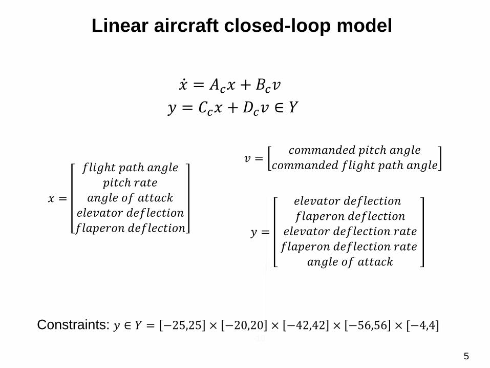
𝑥 =

𝑓𝑙𝑖𝑔ℎ𝑡 𝑝𝑎𝑡ℎ 𝑎𝑛𝑔𝑙𝑒𝑝𝑖𝑡𝑐ℎ 𝑟𝑎𝑡𝑒

𝑎𝑛𝑔𝑙𝑒 𝑜𝑓 𝑎𝑡𝑡𝑎𝑐𝑘𝑒𝑙𝑒𝑣𝑎𝑡𝑜𝑟 𝑑𝑒𝑓𝑙𝑒𝑐𝑡𝑖𝑜𝑛𝑓𝑙𝑎𝑝𝑒𝑟𝑜𝑛 𝑑𝑒𝑓𝑙𝑒𝑐𝑡𝑖𝑜𝑛

𝑣 =𝑐𝑜𝑚𝑚𝑎𝑛𝑑𝑒𝑑 𝑝𝑖𝑡𝑐ℎ 𝑎𝑛𝑔𝑙𝑒

𝑐𝑜𝑚𝑚𝑎𝑛𝑑𝑒𝑑 𝑓𝑙𝑖𝑔ℎ𝑡 𝑝𝑎𝑡ℎ 𝑎𝑛𝑔𝑙𝑒

𝑦 =

𝑒𝑙𝑒𝑣𝑎𝑡𝑜𝑟 𝑑𝑒𝑓𝑙𝑒𝑐𝑡𝑖𝑜𝑛𝑓𝑙𝑎𝑝𝑒𝑟𝑜𝑛 𝑑𝑒𝑓𝑙𝑒𝑐𝑡𝑖𝑜𝑛

𝑒𝑙𝑒𝑣𝑎𝑡𝑜𝑟 𝑑𝑒𝑓𝑙𝑒𝑐𝑡𝑖𝑜𝑛 𝑟𝑎𝑡𝑒𝑓𝑙𝑎𝑝𝑒𝑟𝑜𝑛 𝑑𝑒𝑓𝑙𝑒𝑐𝑡𝑖𝑜𝑛 𝑟𝑎𝑡𝑒

𝑎𝑛𝑔𝑙𝑒 𝑜𝑓 𝑎𝑡𝑡𝑎𝑐𝑘

Constraints: 𝑦 ∈ 𝑌 = −25,25 × −20,20 × −42,42 × −56,56 × [−4,4]

ሶ𝑥 = 𝐴𝑐𝑥 + 𝐵𝑐𝑣

𝑦 = 𝐶𝑐𝑥 + 𝐷𝑐𝑣 ∈ 𝑌

Linear aircraft closed-loop model

5

Ac =[0, 0.0067, 1.341, 0.169, 0.252;

0, -0.869, 43.2, -17.25, -1.577;

0, 0.993, -1.341, -0.169, -0.252;

65, 17.82, 142.3, -30.5, -1.68;

-122,-17.95,-200.6 8.412, -17.89];

Cc = [0, 0, 0, 1, 0;

0, 0, 0, 0, 1;

65, 17.82, 142.3, -30.5, -1.68;

-122, -17.95,-200.6 8.412, -17.89;

0, 0, 1, 0, 0];

Bc = [0, 0;

0, 0;

0, 0;

-57.6, -7.34;

40.4, 81.6];

Dc = [ 0, 0;

0, 0;

-57.6, -7.34;

40.4, 81.6;

0, 0];

Linear aircraft closed-loop model

Closed-loop model (continuous-time) from Sobel and Shapiro, J. Guidance, Control and Dynamics, 8(2) (1985) 181-187.

6

• Convert to a discrete-time model

% Convert the above model to discrete-time using sampling

period of 20 msec

dT = 0.02;

[A,B,C,D]= ssdata( c2d( ss(Ac, Bc, Cc, Dc), dT) );

Discrete-time model

7

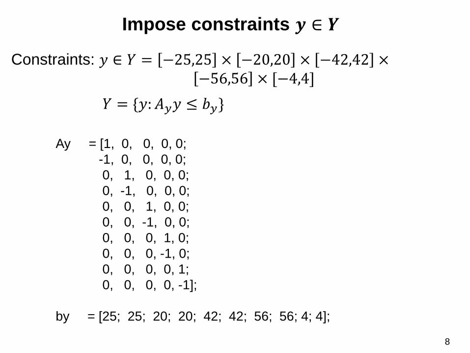
Ay = [1, 0, 0, 0, 0;

-1, 0, 0, 0, 0;

0, 1, 0, 0, 0;

0, -1, 0, 0, 0;

0, 0, 1, 0, 0;

0, 0, -1, 0, 0;

0, 0, 0, 1, 0;

0, 0, 0, -1, 0;

0, 0, 0, 0, 1;

0, 0, 0, 0, -1];

by = [25; 25; 20; 20; 42; 42; 56; 56; 4; 4];

Impose constraints 𝒚 ∈ 𝒀

Constraints: 𝑦 ∈ 𝑌 = −25,25 × −20,20 × −42,42 ×−56,56 × [−4,4]

𝑌 = {𝑦: 𝐴𝑦𝑦 ≤ 𝑏𝑦}

8

Construct ෩𝑶∞ (brute force)

% --- Construct O-infinity (brute force) ----

tstar = 100; % horizon

AOi = [ ]; bOi = [ ];

n = size(A,1);

I = eye(n,n);

for (t = 0:1:tstar),

AOi = [AOi; Ay*(C*inv(I-A)*(I-A^t)*B+D), Ay*(C*A^t)];

bOi = [bOi; by];

end;

% --- Augment tightened steady-state constraints ----

epsi = 0.01;

H = C*inv(I-A)*B+D;

AOi = [AOi; Ay*H,Ay*C*zeros(n,n)];

bOi = [bOi; by*(1-epsi)];

% --- Eliminate redundant inequalities ---

if exist('lp.m','file')>0,

[AOi, bOi] = elimm1(AOi, bOi,1e-12);

end;9

Simulate reference governor

% --- Perform simulations ---

x0 = [0, 0, 0, 0, 0]'; v0 = [0; 0];

[Thist, Vhist, Xhist, Kphist, Rhist] = flow(v0, x0, Rhist, A, B, AOi, bOi);

10

Responses with reference governor

Pitch angle

Flight path angle

𝑟𝜃𝑣𝜃𝜃

𝑟𝛾𝑣𝛾𝛾

≤ 0 ⇒ 𝑐𝑜𝑛𝑠𝑡𝑟𝑎𝑖𝑛𝑡𝑠 𝑠𝑎𝑡𝑖𝑠𝑓𝑖𝑒𝑑

Constraints

Ref. Gov. 𝜿(𝒕)

11

Ay = [1, 0, 0, 0, 0;

-1, 0, 0, 0, 0;

0, 1, 0, 0, 0;

0, -1, 0, 0, 0;

0, 0, 1, 0, 0;

0, 0, -1, 0, 0;

0, 0, 0, 1, 0;

0, 0, 0, -1, 0;

0, 0, 0, 0, 1;

0, 0, 0, 0, -1];

by = [25; 25; 20; 20; 42/4; 42/4; 56/4; 56/4; 4; 4];

Tighten rate limits

12


Pitch angle

Flight path angle


𝑟𝛾𝑣𝛾𝛾

≤ 0 ⇒ 𝑐𝑜𝑛𝑠𝑡𝑟𝑎𝑖𝑛𝑡𝑠 𝑠𝑎𝑡𝑖𝑠𝑓𝑖𝑒𝑑

Constraints


13

Vehicle Rollover ExampleSee vehiclerollover.m

14

Kolmanovsky, I.V., Gilbert, E.G., and Tseng, E., “Constrained control of vehicle

steering,” Proceedings of 2009 IEEE Multi-conference on Systems and Control, St.

Petersburg, Russia, May, 2009, pp. 576-581.

Rollover prevention

• Motivation: Rollover crashes are the leading cause of fatalities

in SUVs.

• Modify driver commanded steering angle if necessary with

Active Front Steer (AFS) system to avoid rollover

• Intervene on other actuators (brakes, etc.) as appropriate

15

Rollover prevention

• Linear model is based on Solmax, Corless and Shorten, “A

methodology for the design of robust rollover prevention

controllers for automotive vehicles: Part 2 - Active steering“,

Proceedings of 2007 American Control Conference, pp.

1606-1611.

• Sample period: 𝑇𝑠 = 10 msec

• Note that tyre force saturation is neglected in the linear

model. This is a more conservative approach, the vehicle is

less likely to rollover if saturation is included.

• Longitudinal speed is treated as a constant parameter

during the maneuver

16

Rollover prevention by modifying steering angle

• Model:

𝑥 𝑡 + 1 = 𝐴𝑥 𝑡 + 𝐵𝛿(𝑡)

𝐴 = 𝐴 𝑣𝑚𝑝𝑠 , 𝐵 = 𝐵(𝑣𝑚𝑝𝑠)

𝑥 =

𝑙𝑎𝑡𝑒𝑟𝑎𝑙 𝑣𝑒𝑙𝑜𝑐𝑖𝑡𝑦 𝑜𝑓 𝐶𝐺, 𝑣𝑦

𝑦𝑎𝑤 𝑟𝑎𝑡𝑒 𝑜𝑓 𝑢𝑛𝑠𝑝𝑟𝑢𝑛𝑔 𝑚𝑎𝑠𝑠, ሶ𝜓

𝑟𝑜𝑙𝑙 𝑟𝑎𝑡𝑒 𝑜𝑓 𝑠𝑝𝑟𝑢𝑛𝑔 𝑚𝑎𝑠𝑠, ሶ𝜙𝑟𝑜𝑙𝑙 𝑎𝑛𝑔𝑙𝑒 𝑜𝑓 𝑠𝑝𝑟𝑢𝑛𝑔 𝑚𝑎𝑠𝑠, 𝜙

𝛿𝑣𝑚𝑝𝑠

=𝑠𝑡𝑒𝑒𝑟𝑖𝑛𝑔 𝑎𝑛𝑔𝑙𝑒 𝑎𝑡 𝑑𝑟𝑖𝑣𝑒𝑟 𝑤ℎ𝑒𝑒𝑙 𝑖𝑛 𝑑𝑒𝑔

𝑙𝑜𝑛𝑔𝑖𝑡𝑢𝑑𝑖𝑛𝑎𝑙 𝑣𝑒ℎ𝑖𝑐𝑙𝑒 𝑠𝑝𝑒𝑒𝑑

(Kolmanovsky, Gilbert, Tseng, 2009)

17

Discrete-time model

• Model:

𝐴 =

0.8646 −0.1382 −0.0379 −0.28690.0379 0.8701 −0.0008 −0.0062−0.1081 0.0595 0.8938 −0.8054−0.0006 0.0003 0.0095 0.9959

𝐵 = 10−3 ×

0.93510.74500.84220.0044

𝑣𝑚𝑝𝑠 = 22.5 𝑚/ sec ⇒

18

Constraints

• Constraints on load transfer ratio:

𝑦 𝑡 = 𝐶𝑥 𝑡 + 𝐷𝑣 ∈ 𝑌 = −0.95, 0.95

𝑦 =1

𝑚𝑔𝐹𝑅 − 𝐹𝐿 =

2

𝑚𝑔𝑇𝑐 ሶ𝜙 + 𝑘 𝜙

𝑦: 𝑙𝑜𝑎𝑑 𝑡𝑟𝑎𝑛𝑠𝑓𝑒𝑟 𝑟𝑎𝑡𝑖𝑜

𝐶 = 0 0 −0.4412 −3.9793

𝐷 = 0.0175

19


Constraints



Steering angle

Path on X-Y plane

𝑟𝜃𝑣𝜃

no R.G.

with R.G.

constraint

violated

20

Anti-rollover reference governor

Bencatel, R., Tian, R., Girard, A., and Kolmanovsky, I.V. “Reference governor strategies

for vehicle rollover avoidance,” IEEE Transactions on Control Systems Technology, vol.

26, no. 6, pp. 1954 – 1969, 2018.

Implementation on a nonlinear model in CARSIM®

Anti-rollover reference governor

• ECG modifies steering and differential braking to prevent rollover

• Nonlinear model

• Vehicle trajectory on X -Y plane with ECG close to the reference trajectory

Anti-rollover extended command governor

Tian, R., Bencatel, R., Girard, A., and Kolmanovsky, I.V., “Coordinated control of active

steering and differential braking using extended command governor for rollover avoidance,”

Proceedings of 2017 ASME Dynamic Systems and Control Conference, Tysons, Virginia,

Paper DSCC2017-5033.

Learning reference governor

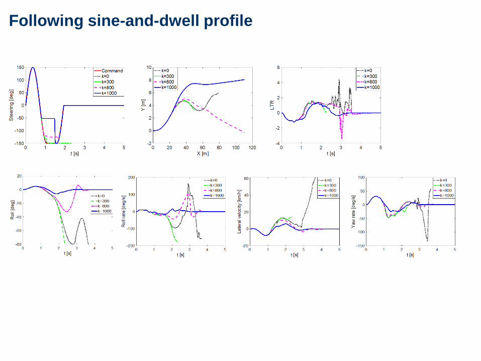
Following sine-and-dwell profile

Constraint violation rate decreases as learning proceeds

Algorithm details and some convergence analysis are in Liu, Li, Rizzo, Garone, Kolmanovsky, and Girard,

Proceedings of 2019 American Control Conference, to appear.

Bypass Valve

HP Check

Valves

LP Check

Valves

Fuel

Load

Reference governor for constraining piston motion in FPE

Zaseck, K., Brusstar, M., and Kolmanovsky, I.V., “Stability, control, and constraint enforcement of piston motion

in a hydraulic free-piston engine,” IEEE Transactions on Control Systems Technology, vol. 25, no. 4,

pp. 1284-1296, 2017.

Free piston engine generator

Xun, G., Kolmanovsky I.V., Garone E., Zaseck K., and Chen H., “Constrained control of free piston engine

generator based on implicit reference governor,” SCIENCE CHINA Information Sciences (SCIS), vol. 61,

no. 7, pp. http://scis.scichina.com, 070203:1–070203:17, 2018

Spacecraft Relative Motion Control

Example

with Linear and Quadratic

Constraints

The example is patterned after Kalabic, U.; Kolmanovsky, I.; Gilbert, E., "Reference

governors for linear systems with nonlinear constraints," 2011 50th IEEE

Conference on Decision and Control, pp.2680-2686, 2011.

see spacecraft_nonlinear_rg.m

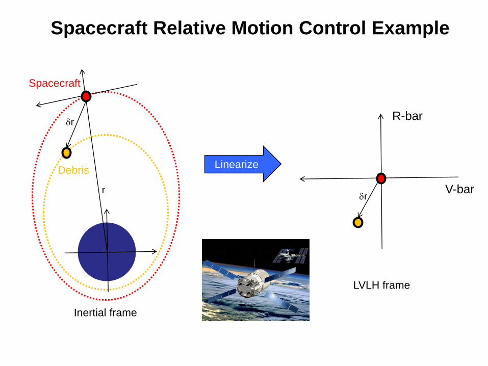
Spacecraft Relative Motion Control Example

Spacecraft

Debris

r

r

Inertial frame

LVLH frame

r

R-bar

V-bar

Linearize

Spacecraft Relative Motion Control Example

x

y

zX

x

y

z

2

2

0 0 0 1 0 0

0 0 0 0 1 0

0 0 0 0 0 1

3 0 0 0 2 0

0 0 0 2 0 0

0 0 0 0 0

cAn n

n

n

𝑥 𝑡 + 1 = 𝐴𝑥 𝑡 + 𝐵𝑢(𝑡)

Relative position (km)

Relative velocity (km/sec)

• Dynamic Model:

0 0 0

0 0 0

0 0 0

1 0 0

0 1 0

0 0 1

cB

𝐴 = 𝑒𝐴𝑐Δ𝑇

𝐵 = 𝑒𝐴𝑐Δ𝑇𝐵𝑐

𝑛 = 0.0011 𝑟𝑎𝑑/𝑠𝑒𝑐 for 350 km altitude Earth orbit

𝑢 𝑡 ∼ "Δ𝑣"

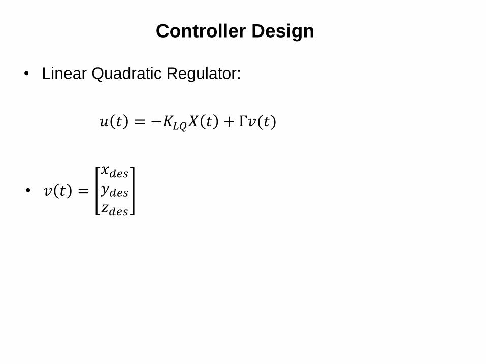
Controller Design

𝑢 𝑡 = −𝐾𝐿𝑄𝑋 𝑡 + Γ𝑣(𝑡)

• Linear Quadratic Regulator:

• 𝑣 𝑡 =

𝑥𝑑𝑒𝑠𝑦𝑑𝑒𝑠𝑧𝑑𝑒𝑠

Constraints [1]

• Line of Sight Cone Constraint configured for the in-track

approach:

𝑥(𝑡)2 + 𝑧(𝑡)2 ≤ 𝑡𝑎𝑛 𝛾 2 𝑦 𝑡 + 0.01 2

𝐶1 𝑡 = 𝑥(𝑡)2 + 𝑧(𝑡)2 − 𝑡𝑎𝑛 𝛾 2 𝑦 𝑡 + 0.01 2 ≤ 0

𝛾 = cone half angle

Constraints [2]

• Thrust / Delta-v Limit assuming single thruster configuration:

𝑢1(𝑡)2 + 𝑢2(𝑡)

2 + 𝑢3 𝑡 2 ≤ 𝑢𝑚𝑎𝑥2

𝐶2(𝑡) = 𝑢1(𝑡)2 + 𝑢2(𝑡)

2 + 𝑢3 𝑡 2 − 𝑢𝑚𝑎𝑥2

𝑢𝑚𝑎𝑥 = 0.001 𝑘𝑚/𝑠𝑒𝑐

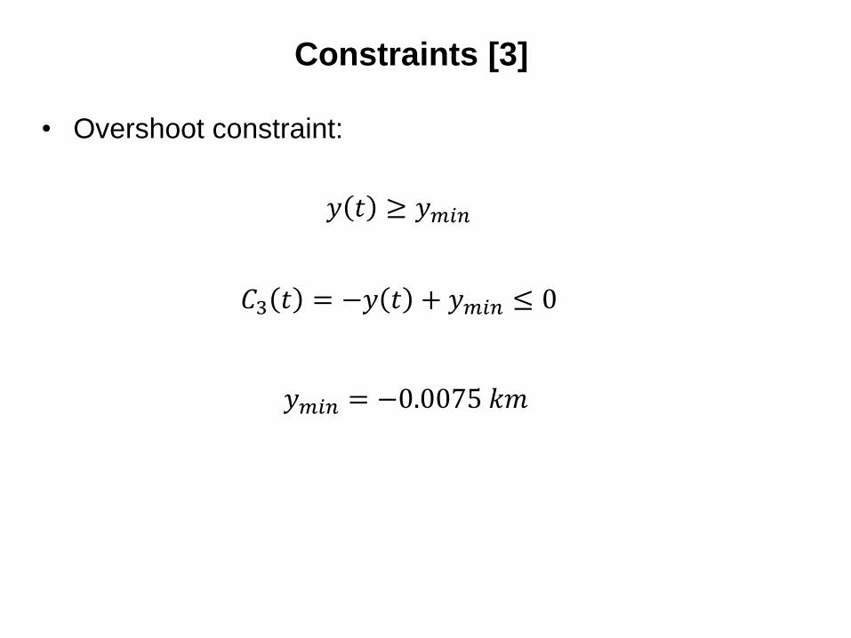
Constraints [3]

• Overshoot constraint:

𝑦 𝑡 ≥ 𝑦𝑚𝑖𝑛

𝐶3 𝑡 = −𝑦 𝑡 + 𝑦𝑚𝑖𝑛 ≤ 0

𝑦𝑚𝑖𝑛 = −0.0075 𝑘𝑚

Responses with the reference governor

𝛥𝑇 = 30, 𝑡∗ = 30 sec,

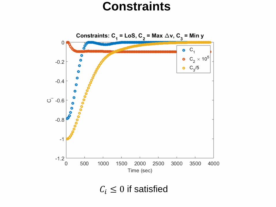
Constraints

𝐶𝑖 ≤ 0 if satisfied

Inputs

Reference governor output

Number of simulation-based response predictions

• Bisection

algorithm is

used

• The case

𝜅 = 1 is

evaluated

first

Incremental RG

Fuel Cell System

45

Load Governor

• Fuel cell loads are controllable

• Load governor (LG): An add-on device that

Enforces constraints (𝜆𝑂2 ≥ 𝜆𝑂2,𝑚𝑖𝑛 , 𝑚𝑂2 ≥ 𝑚𝑂2,𝑚𝑖𝑛)

Minimizes the load tracking error

Deals with uncertainties

Fuel Cell

Stack

State

information

Sun and K., IEEE TCST 13 (6), pp. 991-919, 2005

46

Reference Governor Approach

• A load governor is designed based on the reference governor approach

• The demanded current is altered according to

(0 ≤ ≤ 1) is maximized for load tracking performance subject to

constraints being satisfied for all 𝜏 ≥ 𝑘𝑇 if 𝐼𝑠𝑡 𝜏 = 𝐼𝑠𝑡(𝑘𝑇) for 𝜏 ≥ 𝑘𝑇

• Checking if the constraints are satisfied is accomplished through the

simulation a low-order fuel cell model

TkkTkTII

TkIkTIkTTkIkTI

stst

stdstst

)1(),()(

))1(()()(())1(()(

47

Fuel Cell Model

A 4-state fuel cell model is used for the LG implementation

𝑊𝑥,𝑖𝑛,𝑊𝑥,𝑜𝑢𝑡 calculated from orifice equation, 𝑊𝑂2, 𝑟𝑐𝑡, 𝑊𝑣, 𝑔𝑒𝑛

from the

electrochemical principles, and 𝑊𝑣,𝑚𝑏𝑟 from a phenomenological model

mbrvgenvcaoutvcainvcav

caoutNcainNcaN

rctOcaoutOcainOcaO

smoutinin

sm

asm

WWWWm

WWm

WWWm

TWTWV

Rp

,,_,_,,

_,_,,

,_,_,,

222

2222

)(

48

LG Implementation Details

• An inner loop PI controller is used for O2regulation

• The fuel cell model is augmented with a PI controller

• The 5-state model is simulated over a finite horizon for

constraint violation checking

• Maximum is obtained through bi-sectional search

49

Load Governor with an Observer

• Fuel cell states are not measurable

• LG with an observer

• Measured outputs: supply manifold pressure and cell voltage

State

Observer

psm

vfc

50

Dealing with uncertainties

Sources of uncertainties

• State estimation

• FC model

Temperature

Humidity

Vapor/water diffusion across the membrane

Possible effects:

• Infeasible states

• Constraint violation

51

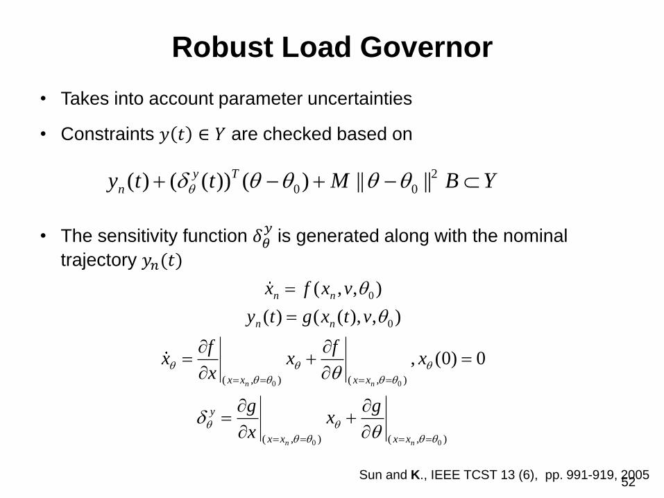
Robust Load Governor

• Takes into account parameter uncertainties

• Constraints 𝑦 𝑡 ∈ 𝑌 are checked based on

• The sensitivity function 𝛿𝜃𝑦

is generated along with the nominal

trajectory 𝑦𝑛(𝑡)

2

0 0( ) ( ( )) ( ) || ||y T

ny t t M B Y

0 0

0 0

0

0

( , ) ( , )

( , ) ( , )

( , , )

( ) ( ( ), , )

, (0) 0

n n

n n

n n

n n

x x x x

y

x x x x

x f x v

y t g x t v

f fx x x

x

g gx

x

Sun and K., IEEE TCST 13 (6), pp. 991-919, 200552

Simulations Setup

LG and RLG are applied to the fuel cell model with

• Large step load changes

• Parameter uncertainties

• Up to 50% change in relative humidity in the supply manifold

• Up to 25kPa in the vapor saturation pressure inside the

cathode (corresponds to about 10oC change in stack

operating temperature)

• Up to 50% change in vapor diffusion coefficient across the

membrane

53

Simulations Results

Nominal system Perturbed system

54

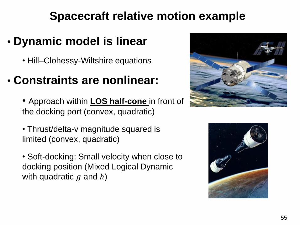
Spacecraft relative motion example

• Dynamic model is linear

• Hill–Clohessy-Wiltshire equations

• Constraints are nonlinear:

• Approach within LOS half-cone in front of

the docking port (convex, quadratic)

• Thrust/delta-v magnitude squared is

limited (convex, quadratic)

• Soft-docking: Small velocity when close to

docking position (Mixed Logical Dynamic

with quadratic 𝑔 and ℎ)

55

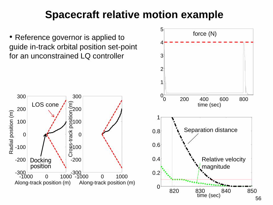
Spacecraft relative motion example

-1000 0 1000-300

-200

-100

0

100

200

300

Ra

dia

l p

ositio

n (

m)

Along-track position (m)-1000 0 1000

-300

-200

-100

0

100

200

300

Cro

ss-t

rack p

ositio

n (

m)

Along-track position (m)

• Reference governor is applied to

guide in-track orbital position set-point

for an unconstrained LQ controller

0 200 400 600 8000

1

2

3

4

5

time (sec)LOS cone

Dockingposition

820 830 840 8500

0.2

0.4

0.6

0.8

1

time (sec)

force (N)

Separation distance

Relative velocity

magnitude

56

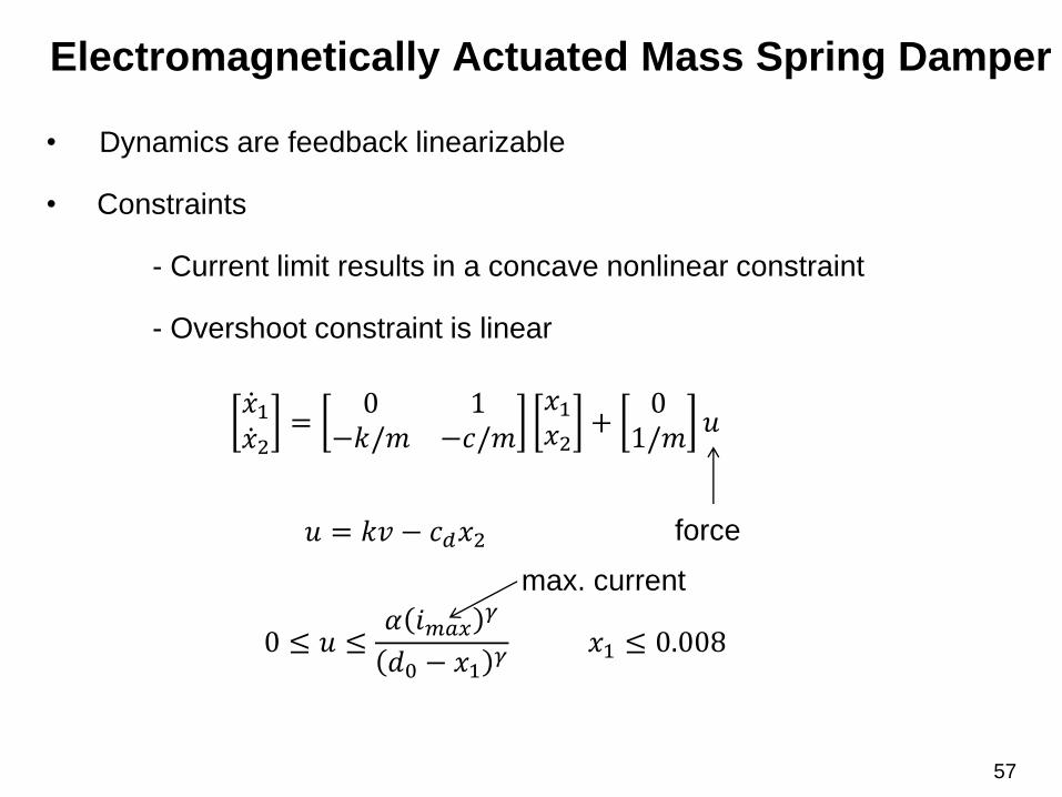
Electromagnetically Actuated Mass Spring Damper

• Dynamics are feedback linearizable

• Constraints

- Current limit results in a concave nonlinear constraint

- Overshoot constraint is linear

ሶ𝑥1ሶ𝑥2

=0 1

−𝑘/𝑚 −𝑐/𝑚

𝑥1𝑥2

+0

1/𝑚𝑢

𝑢 = 𝑘𝑣 − 𝑐𝑑𝑥2

0 ≤ 𝑢 ≤𝛼 𝑖𝑚𝑎𝑥

𝛾

𝑑0 − 𝑥1𝛾

𝑥1 ≤ 0.008

force

max. current

57


0 2 4 60

0.002

0.004

0.006

0.008

0.01

0.012

mass position x1

(m)

time (sec)

unconstrained

imax

=0.5342

imax

=0.365

0 1 2 3 4 50

0.2

0.4

0.6

0.8

current (A)

time (sec)

unconstrained

imax

=0.5342

imax

=0.365

58


• Landing control example

• Voltage limits

• MLD constraints on soft-landing

velocity AND magnetic force

exceeding spring force

𝑑𝑧

𝑑𝑡= 𝑞

𝑑𝑞

𝑑𝑡=

1

𝑚(−𝐹𝑚𝑎𝑔 + 𝑘𝑠 𝑧𝑠 − 𝑧 − 𝑏𝑞)

𝑑𝑖

𝑑𝑡=𝑉𝑐 − 𝑟𝑖 +

2𝑘𝑎𝑖(𝑘𝑏 + 𝑧)2

𝑞

2𝑘𝑠𝑘𝑏 + 𝑧

𝐹𝑚𝑎𝑔 =𝑘𝑎

𝑘𝑏 + 𝑧 2𝑖2

59


60

reference governor applications - lirmm

Documents