refinery hydrogen network optimisation with …
TRANSCRIPT

REFINERY HYDROGEN NETWORK OPTIMISATION
WITH IMPROVED HYDROPROCESSOR MODELLING
A thesis submitted to The University of Manchester for the degree of
Doctor of Philosophy
in the Faculty of Engineering and Physical Sciences
2010
Nan Jia
Centre for Process Integration
School of Chemical Engineering and Analytical Science
brought to you by COREView metadata, citation and similar papers at core.ac.uk
provided by OpenGrey Repository
2
Table of Contents
List of Figures..........................................................................................................6
List of Tables ...........................................................................................................8
Abstract..................................................................................................................10
Declaration.............................................................................................................11
Copyright Statement.............................................................................................12
Acknowledgements................................................................................................13
Chapter 1 Introduction.......................................................................................14
1.1 Basics of Oil Refineries ..........................................................................14
1.2 Emerging Trends on the Oil refining Industry........................................16
1.2.1 Environmental Concerns on Refinery.................................................16
1.2.2 Hydroprocessing for Heavy Crude......................................................18
1.3 Hydroprocessing Technology .................................................................20
1.3.1 Hydrotreating Process .........................................................................21
1.3.2 Hydrocracking Process........................................................................22
1.3.3 Hydrogen Resources in Refineries......................................................23
1.3.4 Hydrogen Network..............................................................................25
1.4 Summary and Thesis Structure ...............................................................26
Chapter 2 Literature Review..............................................................................28
2.1 Hydrogen Management with Thermodynamics Analysis.......................28
2.2 Cost and Value Composite Curves for Hydrogen Management.............30
2.3 Hydrogen Pinch Analysis........................................................................31
2.3.1 Hydrogen Source and Sink..................................................................32
2.3.2 Hydrogen Composite Curve and Surplus Curve.................................33
2.3.3 Hydrogen Purity Analysis ...................................................................36
2.3.4 Limitation of Hydrogen Pinch Analysis .............................................37

3
2.4 Applications and Extensions of Hydrogen Pinch Analysis.....................38
2.5 MINLP H2 Network Optimisation with Purifier Selection Strategy......42
2.5.1 Inclusion of Pressure Consideration....................................................43
2.5.2 Strategy of Purifier Selection..............................................................45
2.5.3 H2 Plant Integration ............................................................................46
2.5.4 Other Systematic Optimisation Methodologies ..................................50
2.6 Molecular Modelling of Hydroprocessors ..............................................51
2.7 Rigorous Optimisation of Hydrogen Networks with Impurity
Considerations.....................................................................................................52
2.8 Modelling and Optimisation of Hydrogen Networks for Multi-period
Operation.............................................................................................................54
2.8.1 Mathematic Formulation.....................................................................55
2.8.2 Optimisation Framework ....................................................................55
2.9 Summary .................................................................................................56
Chapter 3 ..Modified Modelling and Optimisation Methodology for Binary H2
Networks………………………………………………………………………….58
3.1 Introduction .............................................................................................58
3.2 Sensitivity Analysis of Variable H2/Oil Ratio and H2 Partial Pressure on
Hydroprocessor Operation ..................................................................................60
3.2.1 H2/Oil Ratio and H2 Partial Pressure vs Product Yield .....................60
3.2.2 H2/Oil Ratio and H2 Partial Pressure vs H2 Recycle/Purge...............62
3.2.3 Conclusions from the Sensitivity Analysis .........................................69
3.3 Improved Hydrogen Network Formulation and Optimisation
Methodology .......................................................................................................70
3.3.1 Mass Balance of Hydrogen Producers ................................................70
3.3.2 Mass Balance of H2 Headers ..............................................................71
3.3.3 Consumer Reactor Inlets .....................................................................71
3.3.4 Consumer Flash Calculation ...............................................................73
3.3.5 Mass Balance of Purifiers ...................................................................74
3.3.6 Power Consumption of Compressors..................................................75
3.3.7 Summary of Binary H2 Network Modelling ......................................75

4
3.4 Optimisation Methodology .....................................................................77
3.4.1 Key Assumptions ................................................................................77
3.4.2 Optimisation Framework ....................................................................78
3.5 Case study ...............................................................................................80
3.5.1 Software Tool......................................................................................80
3.5.2 Hydrogen Network Base Case with Pinch Analysis ...........................81
3.5.3 H2 Network Operating Cost ...............................................................85
3.5.4 Optimisation Solutions Analysis and Comparison .............................87
3.5.5 Solutions Comparison .........................................................................92
3.6 Summary .................................................................................................93
Chapter 4 Detailed Modelling and Validation of H2 Consumers ...................95
4.1 Introduction .............................................................................................95
4.2 Improved Hydrogen Consumer Model ...................................................96
4.2.1 Feed Mixing ........................................................................................98
4.2.2 Hydroprocessing Reaction ................................................................100
4.2.3 Flash Separation ................................................................................102
4.2.4 Detailed H2 Consumer Modelling Summary....................................104
4.3 Integrated Flash Calculation with Constant K-values...........................105
4.3.1 Introduction of Integrated Flash Calculation ....................................105
4.3.2 Results of Constant K-values Verification........................................107
4.4 Summary ...............................................................................................112
Chapter 5 Multi-component Optimisation for H2 networks ........................114
5.1 Overall Hydrogen Network Modelling and Optimisation ....................114
5.1.1 Hydrogen Producer Model................................................................114
5.1.2 Site Fuel Balance...............................................................................115
5.1.3 Overall Multi-component H2 Network Modelling ...........................117
5.1.4 H2 Network Superstructure ..............................................................118
5.1.5 H2 Network Optimisation Framework..............................................120
5.1.6 Pseudo-components ..........................................................................122
5.1.7 Selection of Optimisation Solvers.....................................................124

5
5.2 Case Study.............................................................................................124
5.2.1 Base Case ..........................................................................................125
5.2.2 Hydrogen Pinch Analysis..................................................................131
5.2.3 Optimisation and Solution Analysis .................................................132
5.3 Methodology Comparison with Simulated Annealing..........................138
5.3.1 Brief Introduction of Simulated Annealing.......................................139
5.3.2 SA Parameters...................................................................................140
5.3.3 SA Moves..........................................................................................141
5.3.4 Modelling Comparison with NLP Methodology ..............................142
5.3.5 Case Study Comparison ....................................................................143
5.3.6 Methodology Comparisons ...............................................................145
5.4 Summary ...............................................................................................146
Chapter 6 Conclusions and Future work........................................................148
6.1 Conclusions ...........................................................................................148
6.2 Future Work ..........................................................................................149
Nomenclature…………………………………………………………………...150
References...…………………………………………………………………….154
Appendix A Binary H2 network optimisation program codes (GAMS)…..161
Appendix B Constant K-values simulation for verification ..........................171
Appendix C Multi-component H2 network
optimisation program codes (GAMS) .............................................................. .175

6
List of Figures
Figure 1.1 A general oil refinery structure (Beychok, 2008)..........................15
Figure 1.2 U.S. Trend of sulphur content in crude oil (U.S. Energy
Information Administration, 2010) .........................................................18
Figure 1.3 A typical hydrotreater flowsheet (Beychok, 2006)........................22
Figure 1.4 A typical hydrocracker flowsheet (Hiller, 1987)...........................23
Figure 1.5 A typical refinery structure flowsheet (Singh, 2006) ....................25
Figure 2.1The thermodynamic mountain (Simpson, 1984) ............................29
Figure 2.2 An example of value composite curves (Towler et al., 1996) .......30
Figure 2.3 A simplified model of a hydrogen consumer ...............................32
Figure 2.4 Hydrogen composite curve ............................................................34
Figure 2.5 Hydrogen surplus curve.................................................................34
Figure 2.6 Hydrogen pinch point ....................................................................35
Figure 2.7 Purity increase impace on hydrogen pinch analysis ......................36
Figure 2.8 Hydrogen purification strategy based on pinch analysis ...............37
Figure 2.9 Hydrogen network superstucture (Liu, 2002)................................43
Figure 2.10 Hydrogen purifer involved into superstucture (Liu, 2002)..........44
Figure 2.11 MINLP problem relaxation methodology ...................................45
Figure 2.12 Simplified hydrogen model simulation (Liu, 2002) ....................47
Figure 2.13 Linear hydrogen plant model (Liu, 2002)....................................48
Figure 2.14 Superstructure for integration of hydrogen plant (Liu, 2002) .....48
Figure 2.15 Hydrogen network optimisation framework................................53
Figure 2.16 Hydrogen network optimisation framework................................56
Figure 3.1 Fixed reactor inlet conditions ........................................................58
Figure 3.2 An example of a hydrogen network with a header ........................59
Figure 3.3 The hydrocracker model for verification.......................................63
Figure 3.4 The hydrocracker model for verification in ASPEN PLUS ..........64
Figure 3.5 The recycle/purge purity vs H2 partial pressure............................65
Figure 3.6 The purge flowrate vs H2 partial pressure.....................................66
Figure 3.7 The recycle flowrate vs H2 partial pressure ..................................66
Figure 3.8 The recycle/purge purity vs H2/Oil ratio&H2 partial pressure .....68
Figure 3.9 The purge flowrate vs H2/Oil ratio&H2 partial pressure ..............68
Figure 3.10 The recycle flowrate vs H2/Oil ratio&H2 partial pressure..........69

7
Figure 3.11 Binary hydrogen network optimisation framework.....................79
Figure 3.12 The hydrogen network base case.................................................81
Figure 3.13 Hydrogen surplus curve for the base case ...................................83
Figure 3.14 Idea of hydrogen purification below the pinch............................85
Figure 3.15 The optimised hydrogen network of solution 1...........................87
Figure 3.16 The optimised hydrogen network of solution 2...........................89
Figure 3.17 The optimised hydrogen network of solution 3...........................91
Figure 4.1 The improved hydrogen consumer model .....................................97
Figure 4.2 Model construction of a H2 consumer ..........................................98
Figure 4.3 Sink mass balances ........................................................................99
Figure 4.4 Reactor model..............................................................................100
Figure 4.5 Flash separation model ................................................................102
Figure 4.6 The improved hydrocracker model..............................................105
Figure 4.7 Constant K-values verification procedure ...................................106
Figure 5.1 Short-cut hydrogen producer model ............................................114
Figure 5.2 An example of site fuel model for a hydrogen network ..............116
Figure 5.3 An example of hydrogen network superstructure........................120
Figure 5.4 The Multi-component hydrogen network optimisation framework
...............................................................................................................121
Figure 5.5 Multi-component hydrogen network base case ...........................125
Figure 5.6 Hydrogen network composite curves ..........................................131
Figure 5.7 Hydrogen network surplus curve.................................................131
Figure 5.8 The optimal solution for multi-component optimisation.............134
Figure 5.9 SA moves for hydrogen network optimisation............................141
Figure 5.10 SA moves for hydrogen network optimisation..........................142
Figure 5.11 SA optimisation solution ...........................................................144
8
List of Tables
Table 1.1 U.S. Sulphur content of crude oil....................................................17
Table 1.2 2007 World crude characteristics selection ....................................19
Table 1.3 Typical hydrogen consumption data ...............................................20
Table 1.4 Typical hydrogen production data ..................................................24
Table 3.1 Product yield under different H2 partial pressure...........................61
Table 3.2 Product yield under different reaction pressure ..............................62
Table 3.3 Variable H2/Oil ratio and H2 partial pressure strategy verification
simulation scenarios ................................................................................64
Table 3.4 Variable H2/Oil ratio and H2 partial pressure strategy verification
simulation scenarios ................................................................................67
Table 3.5 Reactor inlet conditions for the base case.......................................83
Table 3.6 costs of hydrogen production and utility.........................................86
Table 3.7 Reactor inlet conditions comparison for Solution 1........................88
Table 3.8 Reactor inlet conditions comparison for Solution 2........................90
Table 3.9 Reactor inlet conditions comparison for solution 3 ........................92
Table 3.10 Reactor inlet conditions comparison for solution 3 ......................93
Table 4.1 Typical operating temperature and pressure for a hydrotreater ....108
Table 4.2 Constant K-values verification base case......................................109
Table 4.3 Flash model simulation results......................................................110
Table 4.4 Flash model base case and simulations comparison .....................111
Table 5.1 Properties of pseudo components .................................................123
Table 5.2 Details of network connections for each H2 consumer ................126
Table 5.3 Flash Operating conditions for each hydrogen consumer.............126
Table 5.4 Detailed data of liquid feedstock for each H2 consumer ..............127
Table 5.5 Detailed data of H2 consumers for base case ...............................128
Table 5.6 Base case data verification in HYSYS..........................................130
Table 5.7 Constant K-values strategy verification........................................132
Table 5.8 Connections overview for the optimal solution ............................134
Table 5.9 Detailed data of H2 consumers for optimal solution ....................135
Table 5.10 Data comparison between base case and optimisation results....137
Table 5.11 Reactor inlet conditions comparison...........................................138
Table 5.12 SA parameters selection..............................................................143

9
Table 5.13 Network connections summary...................................................144
Table 5.14 Detailed data for SA optimal solution.........................................145
Table 5.15 Detailed data for optimal solution...............................................146

10
Abstract
Heavier crude oil, tighter environmental regulations and increased heavy-end
upgrading in the petroleum industry are leading to the increased demand for
hydrogen in oil refineries. Hence, hydrotreating and hydrocracking processes now
play increasingly important roles in modern refineries. Refinery hydrogen
networks are becoming more and more complicated as well. Therefore,
optimisation of overall hydrogen networks is required to improve the hydrogen
utilisation in oil refineries.
In previous work for hydrogen management many methodologies have been
developed for H2 network optimisation, all with fixed H2/Oil ratio and H2 partial
pressure for H2 consumers, which may be too restrictive for H2 network
optimisation. In this work, a variable H2/Oil and H2 partial pressure strategy is
proposed to enhance the H2 network optimisation, which is verified and integrated
into the optimisation methodology. An industrial case study is carried out to
demonstrate the necessity and effectiveness of the approach.
Another important issue is that existing binary component H2 network
optimisation has a very simplistic assumption that all H2 rich streams consist of H2
and CH4 only, which leads to serious doubts about the solution’s validity. To
overcome the drawbacks in previous work, an improved modelling and
optimisation approach has been developed. Light-hydrocarbon production and
integrated flash calculation are incorporated into a hydrogen consumer model. An
optimisation framework is developed to solve the resulting NLP problem. Both the
CONOPT solver in GAMS and a simulated annealing (SA) algorithm are tested to
identify a suitable optimisation engine. In a case study, the CONOPT solver out-
performs the SA solver. The pros and cons of both methods are discussed, and in
general the choice largely depends on the type of problems to solve.

11
Declaration
No portion of the work referred to in this thesis has been submitted in support of an
application for another degree or qualification of this or any other university or
other institution of learning.
Nan Jia

12
Copyright Statement
[i] The author of this thesis (including any appendices and/or schedules to
this thesis) owns any copyright in it (the “Copyright”) and he has given
The University of Manchester the right to use such Copyright for any
administrative, promotional, educational and/or teaching purposes.
[ii] Copies of this thesis, either in full or in extracts, may be made only in
accordance with the regulations of the John Rylands University Library
of Manchester. Details of these regulations may be obtained from the
Librarian. This page must form part of any such copies made.
[iii] The ownership of any patents, designs, trade marks and any and all
other intellectual property rights except for the Copyright (the
“Intellectual Property Rights”) and any reproductions of copyright
works, for example graphs and tables (“Reproductions”), which may be
described in this thesis, may not be owned by the author and may be
owned by third parties. Such Intellectual Property Rights and
Reproductions cannot and must not be made available for use without
the prior written permission of the owner(s) of the relevant Intellectual
Property Rights and/or Reproductions.
[iv] Further information on the conditions under which disclosure,
publication and exploitation of this thesis, the Copyright and any
Intellectual Property Rights and/or Reproductions described in it may
take place is available from the Head of School of Chemical
Engineering & Analytical Science.

13
Acknowledgements
I would like to express my sincerest gratitude to my supervisor, Dr Nan Zhang,
who has supported me throughout my research with his knowledge and patience
over the past few years, without which the thesis would not have been completed. I
genuinely appreciate all the discussions we had which did help me all the way
through, for which I am extremely grateful.
I wish to thank Centre for Process Integration and School of Chemical Engineering
and Analytical Science for offering me the study opportunity and the finical
support. I also thank Prof Robin Smith and Dr Qiying Yin for their support and
assistance.
It has been a great pleasure working along with all of the CPI fellow students. It is
an honour for me to thank Yongwen, Zixin, Xuesong, Donghui, Yuhang, Lu,
Michael, Imran, Yurong, Sonia, Yadira, Leorelis, Kok Siew, Yufei, Muneeb,
Ankur, Bostjan, Yanis and Anestis for their effort of creating such fabulous
academic and social environment in CPI.
I owe my deepest gratitude to my parents and my wife for their continuous
understanding, unconditional support, and unforgettable love. I take this
opportunity to thank my family, who are behind me for everything and mean
everything to me.

14
Chapter 1 Introduction
1.1 Basics of Oil Refineries
With the rising crude oil price and the growing transportation fuel market, it
is becoming a trend that refineries convert as much crude oil as possible
into transportation fuels, such as gasoline, diesel and jet fuel etc. Besides
this, crude oil can also be further processed into feed stock for
petrochemical plants to produce valuable products such as ethylene,
polyethylene and so on. Although this market is increasing rapidly, it is still
far behind the transportation fuel production in overall revenue distribution.
Unsurprisingly, refineries all over the world are always looking for new
ways or new technology to improve the process performance as well as the
quality of products in order to increase their profitability. To achieve the
goal of the highest possible conversion from crude oil into transportation
fuel, many newly developed methodologies and technologies have adopted
advanced hydroprocessing technology. The implementation of
hydroprocessing technology also helps refineries to overcome the
increasingly stricter specifications of petroleum products.
Refineries vary in capacity and configurations, and the overall flowsheet of
a refinery can be very complicated and huge. Figure 1.1 shows a typical
modern refinery structure. Basically refineries intake crude oil and then
process it through various processes so as to produce different kinds of
products.
Crude first gets heated before going into the atmospheric distillation
column (Atmospheric Distillation Unit, ADU), where the distillation happens
in different stages inside a tower with different temperatures and separates
crude oil into wet gas, light straight run naphtha, heavy naphtha, kerosene,
atmospheric gas oil and atmospheric residue.

15
Figure 1.1 A general oil refinery structure (Beychok, 2008)
As an extraction of ADU, light naphtha is hydrotreated and then sent into
isomerisation to produce isomerates for gasoline blending. Heavy naphtha
is also hydrotreated (NHT) firstly before it goes to catalytic reformer (CCR),
where the octane number is improved and the reformate goes to the
gasoline blending pool as well. Kerosene comes through a kerosene
hydrotreater (KHT) to produce jet fuel. Diesel oil is produced after diesel
distillates have been hydrotreated.

16
Atmospheric residue is further processed in the Vacuum Distillation Unit
(VDU) where it is separated into light vacuum gas oil, heavy vacuum gas
oil, and vacuum residue. It is generally considered to use light vacuum gas
oil as the feed stock of fluid catalytic cracking (FCC) and heavy vacuum
gas oil as the feed stock of hydrocracker unit (HCU). Similarly, within FCC
and HCU, the heavy petroleum molecules are cracked into lower molecular
weight compounds within the boiling ranges of gasoline and distillate fuels.
FCC gasoline is hydrodesulphurised and blended into the gasoline pool, as
is the hydrocracker naphtha and middle distillates. The alkylation unit
produces high-octane alkylate that can be blended into gasoline to improve
the octane number of the gasoline pool.
The Vacuum residue (VR) needs to be treated. The Delayed Coker Unit
(DCU) is used to process VR, and coker naphtha, coking gas oil and coke
is produced. Coker naphtha is hydrotreated and used as petrochemical
naphtha or the CCR feedstock, while coke can be sold straight away as
one of refinery’s products.
Wet gas generated from FCC, DCU, HCU and other units are sent to a gas
processing unit, where it can be separated and light naphtha stabilized to
produce refinery fuel gas and liquid petroleum gas (LPG). After treating
and blending, the refinery can produce gasoline, jet fuel, diesel and
lubricating base oil, etc.
1.2 Emerging Trends on the Oil refining Industry
1.2.1 Environmental Concerns on Refinery
It has been a tendency that crude oil is becoming heavier and higher in
sulphur. The difficulties of processing heavy oil or high-sulphur crude have
been increasing for years and refiners are always perusing better
technology to overcome these problems. Table 1.1 gives an overview of
U.S. crude characteristics from 1985 to 2009 (U.S. Energy Information

17
Administration, 2010) including statistics about sulphur content and API
gravity. The weight percentage of sulphur rises year by year steadily. The
total amount of sulphur content has increased by around 53.8% from
0.91% in 1995 to 1.4% in 2009, which is quite significant.
Table 1.1 U.S. Sulphur content of crude oil
Year API Gravity U.S. Sulphur Content
of Crude Oil (wt%)
1985 32.46 0.91
1986 32.33 0.96
1987 32.22 0.99
1988 31.93 1.04
1989 32.14 1.06
1990 31.86 1.1
1991 31.64 1.13
1992 31.32 1.16
1993 31.30 1.15
1994 31.39 1.14
1995 31.30 1.13
1996 31.14 1.15
1997 31.07 1.25
1998 30.98 1.31
1999 31.31 1.33
2000 30.99 1.34
2001 30.49 1.42
2002 30.42 1.41
2003 30.61 1.43
2004 30.18 1.43
2005 30.20 1.42
2006 30.44 1.41
2007 30.42 1.43
2008 30.21 1.47
2009 30.37 1.4
(U.S. Energy Information Administration, 2010)
In the meantime, refiners are facing much tighter and stricter transportation
fuel specification standards and environmental regulations. Tougher rules
have been applied on specifications of gasoline and diesel both in the
European Union and United States to reduce smog-forming and other
pollutants from vehicle emissions. For instance, the maximum sulphur limit
for diesel in the European Union decreased to 10ppm compared with
50ppm in 2005 (Europa.eu, 2007). In the United States a similar thing
happened. In 1993 the maximum sulphur limit for diesel was 500ppm and it
has been reduced by 10 times in just 12 years to only 15ppm in 2006 (US
Environmental Protection Agency, 2006). As can be predicted from these

18
numbers the quality regulations on fuel are becoming stricter and stricter
resulting from environmental concerns. Plotting the sulphur content against
years, Figure 1.2 indicates the increase trend of sulphur content in the U.S.
crude oil.
Figure 1.2 U.S. Trend of sulphur content in crude oil (U.S. Energy
Information Administration, 2010)
Hence, hydrogen is required considerably more in refineries for
desulphurisation, denitrogenation and other usage. Along with the growing
transportation fuel market, the hydrogen availability has become a focal
point in modern refineries. Lower sulphur fuel would need more hydrogen
for hydrotreating processes. Meanwhile as a by-product of catalytic
reformer, the amount of hydrogen produced is also affected by milder
operation severity resulting from stricter fuel specifications. It is reported
that in Europe and US, the hydrogen demand rises from 10MMNm3/h to
15MMNm3/h while the rate of by-product hydrogen and recovery from off-
gas is decreased from 75% to 35% from 1995 to 2005.
Moreover, hydrogen production is now under pressure as a result of recent
rules of cutting down the greenhouse gas emissions. With increased
concerns on global warming and controlling of greenhouse gas emissions,
it can be predicted that the refinery hydrogen production will become more
expensive and face much stringent standards.
1.2.2 Hydroprocessing for Heavy Crude
World’s crude oil is estimated to become heavier and contain more sulphur.
19
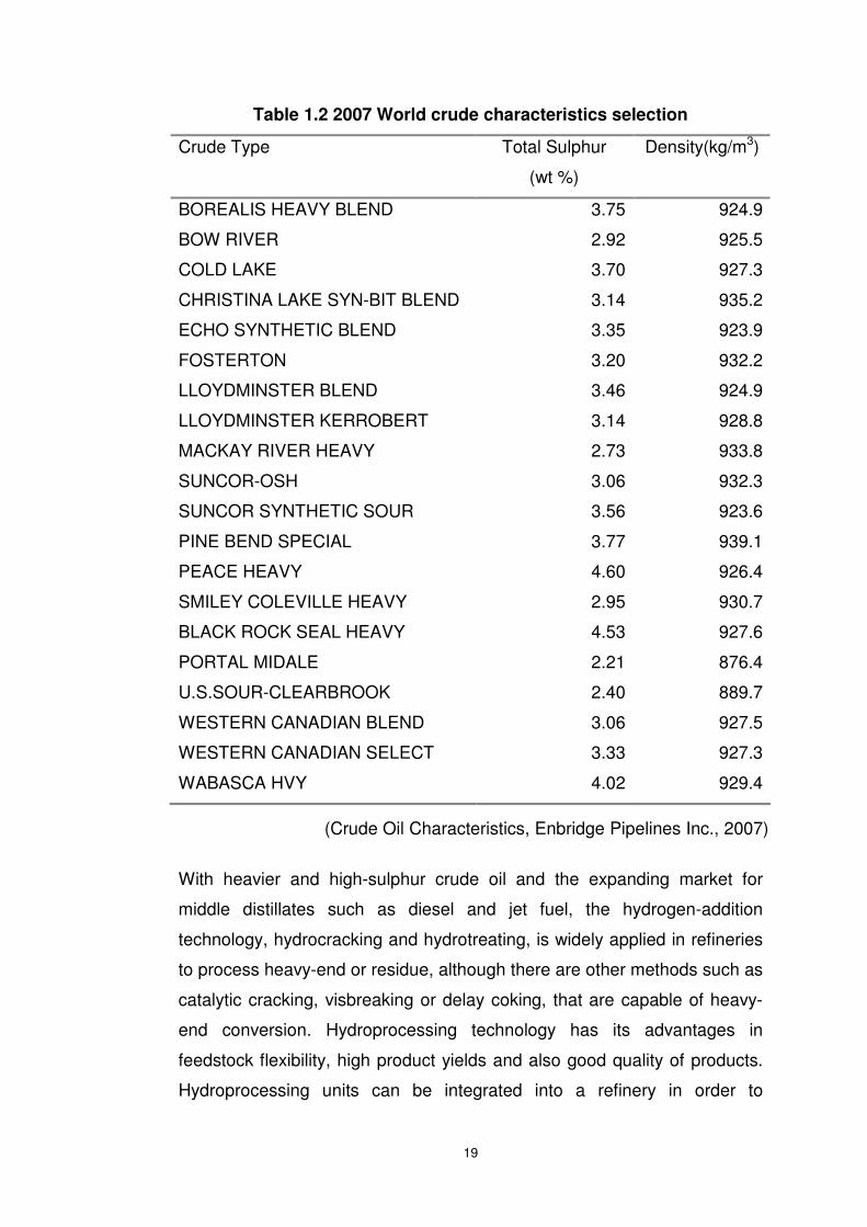
Table 1.2 2007 World crude characteristics selection
Crude Type Total Sulphur
(wt %)
Density(kg/m3)
BOREALIS HEAVY BLEND 3.75 924.9
BOW RIVER 2.92 925.5
COLD LAKE 3.70 927.3
CHRISTINA LAKE SYN-BIT BLEND 3.14 935.2
ECHO SYNTHETIC BLEND 3.35 923.9
FOSTERTON 3.20 932.2
LLOYDMINSTER BLEND 3.46 924.9
LLOYDMINSTER KERROBERT 3.14 928.8
MACKAY RIVER HEAVY 2.73 933.8
SUNCOR-OSH 3.06 932.3
SUNCOR SYNTHETIC SOUR 3.56 923.6
PINE BEND SPECIAL 3.77 939.1
PEACE HEAVY 4.60 926.4
SMILEY COLEVILLE HEAVY 2.95 930.7
BLACK ROCK SEAL HEAVY 4.53 927.6
PORTAL MIDALE 2.21 876.4
U.S.SOUR-CLEARBROOK 2.40 889.7
WESTERN CANADIAN BLEND 3.06 927.5
WESTERN CANADIAN SELECT 3.33 927.3
WABASCA HVY 4.02 929.4
(Crude Oil Characteristics, Enbridge Pipelines Inc., 2007)
With heavier and high-sulphur crude oil and the expanding market for
middle distillates such as diesel and jet fuel, the hydrogen-addition
technology, hydrocracking and hydrotreating, is widely applied in refineries
to process heavy-end or residue, although there are other methods such as
catalytic cracking, visbreaking or delay coking, that are capable of heavy-
end conversion. Hydroprocessing technology has its advantages in
feedstock flexibility, high product yields and also good quality of products.
Hydroprocessing units can be integrated into a refinery in order to

20
maximize profits.
Table 1.3 Typical hydrogen consumption data
Process %wt on feed %wt on crude
HT Str. Run Naphtha 0.05 0.01
HT FCC/TC Naphtha 1 0.05-1
HT Kerosene 0.1 0.01-0.02
HDS LS Gasoline to 0.2% S 0.1 0.03
HDS HS Gasoline to 0.2% S 0.3 0.04
HDS LS Gasoline to 0.05% S 0.15 0.04
HDS HS Gasoline to 0.05% S 0.35 0.05
HDS FCC/TC Gasoline 1 0.1
Cycle oils hydrogenation 3 0.3
Hydrocracking VGO 2-3 0.5-0.8
Deep residue conversion 2-3.5 1-2
Lamber et al. (1994)
Table 1.3 shows that vacuum distillates and residue hydroprocessing
account for most of the hydrogen consumption in refinery processes.
The wide implementation of hydroprocessing technology leads to
significantly increased demand for hydrogen. Therefore hydrogen
management is focused on making the best use of limited hydrogen
resources, and it has become essential for modern refineries to optimise its
operation.
1.3 Hydroprocessing Technology
Hydrogen is added into molecules of oil streams by hydroprocessing units.
The aims of adding hydrogen by different hydrotreating processes are
shown below:

21
• Removing non-hydrocarbon impurities such as sulphur, nitrogen and
metals in order to produce good quality products
Chemistry:
- Hydrodesulphurisation
Ethanethiol + Hydrogen → Ethane + Hydrogen sulphide
C2H5SH + H2 → C2H6 + H2S
- Hydrodenitrogenation
Pyridine + Hydrogen → Pentane + Ammonia
C5H5N + 5H2 → C5H12 + NH3
• Improving the operation of a downstream refining unit
• Saturating olefins and aromatics in order to improve product colour,
stability and make premium quality lubricating oils
Chemistry:
- Olefins Saturation
Pentene + Hydrogen → Pentane
C5H10 + H2 → C5H12
• Cracking heavy, low-value oils into lighter, higher-value products via
hydrocracking
Without changing the density and boiling point of oil streams significantly,
hydrotreating processes generally remove hazardous materials in the
streams. In a hydrocracking process, the main reactions involve
hydrogenation, cracking and isomerisation, which change the size and
shape of molecules.
1.3.1 Hydrotreating Process
A typical hydrotreating process flowsheet is shown in Figure 1.3.

22
Figure 1.3 A typical hydrotreater flowsheet (Meyers, 2003)
• Application: Reduction of the sulphur, nitrogen and metals content
of naphtha, kerosene, diesel or gas oil streams.
• Products: Low-sulphur products for sale or further processing.
• Description: Single or multibed catalytic treatment of hydrocarbon
liquids in the presence of hydrogen converts organic sulphur to H2S
and organic nitrogen to ammonia. Naphtha treating normally takes
place in the vapour phase, while heavier oils usually operate in
mixed-phase.
• Operating conditions: 561K to 672K, 2.76MPa to 10.34MPa
reactor conditions (Refining Processes Handbook, 2004).
1.3.2 Hydrocracking Process
Figure 1.4 shows a typical hydrocracker flowsheet.

23
Make-upHydrogen
RecycleHydrogen
Feed
Reactor
Water
H2SRemoval
Lean Amine
Rich Amine
Sour Water
Gas
Treatedproduct
Purge
Figure 1.4 A typical hydrocracker flowsheet (Hiller, 1987)
• Application: Upgrade vacuum gas oil alone or blended with various
feed stocks, light cycle oil, deasphalted oil, and visbreaker or coker-
gas oil for instance.
• Products: Middle distillates, low-sulphur fuel oil, FCC feed, lube oil
base stocks.
• Description: By using refining and hydrocracking catalyst,
hydrocracker is able to process heavy oil cracking big molecular into
smaller ones. The process consists of: reaction section, gas
separator, stripper and product fractionator.
• Operating conditions:
Reactor temperature, K 658-722
Reactor pressure, MPa 9.66-24.14
H2 partial pressure, MPa 6.89-18.62
(Refining Process Handbook, 2004)
1.3.3 Hydrogen Resources in Refineries
A few hydrogen sources are available in modern refineries such as
catalytic reforming, steam reforming and hydrogen recovery from off-gas.
Some refineries with high-demand hydrogen also have hydrogen plants to
produce hydrogen.

24
A Catalytic reformer is a very common unit that produces hydrogen. During
reforming of hydrocarbon molecules a large amount of hydrogen is
produced as a by-product. The off-gas is very rich in hydrogen and can be
sent to a hydrotreater or a hydrocracker directly if the purity is high enough.
Otherwise the gas will be purified first by a hydrogen purifier such as PSA
or membrane and then sent to hydroprocessors.
Table 1.4 Typical hydrogen production data
Process %wt on feed %wt on crude
Continuous Regeneration Reformer
0.05 0.01
Semi-regeneration Reformer 1 0.05-1
Residue Gasification 0.1 0.01-0.02
Catalytic Cracking 0.1 0.03
Thermal Cracking 0.3 0.04
Ethylene Cracker 0.15 0.04
Steam Reformer 0.35 0.05
Lamber et al. (1994)
Light distillates, such as LPG or light naphtha can be converted into high
purity hydrogen through steam reforming. Table 1.4 summarised typical
hydrogen production data.
Off-gas recycle is another important feature of hydrogen utilization in
refineries. Apart from an internal recycle built in hydroprocessing units
themselves, there are many possible external recycles around refinery
processes. Hydrogen is rich in off-gas of many processes such as delayed
coking and catalytic cracking. However the purity of off-gas may not be
high enough. So sometimes a purifier is introduced to improve the
concentration of hydrogen before sending it to a hydrogen consumer.
Purifiers can also remove hazards and impurities in hydrogen, which allows
hydrogen consumers to use it in a more efficient way.

25
Although hydrogen resources in refineries look abundant, the rapidly
increasing hydrogen demand is causing a hydrogen shortage. Therefore,
hydrogen management is aiming to make the best use of hydrogen
resources in order to satisfy increased demand and improve profitability.
1.3.4 Hydrogen Network
Obviously, there are many processes in the refinery dealing with hydrogen.
If we separate these hydroprocessors and hydrogen plants from other
refinery processes, a refinery hydrogen network can be formed. In a
hydrogen network, the most common hydrogen consumers are
hydrotreaters and hydrocrackers. For hydrogen producers, there can be a
hydrogen plant, a catalytic reformer or an ethylene pant. Figure 1.5 gives
us an example of a middle-scale refinery hydrogen network with 2
hydrogen producers and 6 hydrogen consumers.
HCU DHT KHT
CNHT NHT
HDA
H2 Plant CRU
Fuel
Figure 1.5 A typical refinery structure flowsheet (Singh, 2006)
The processes involved in this hydrogen network can be summarised as
follows:
26
• Hydrogen producers: H2 plant and catalytic reformer (CRU)
• Hydrogen consumers: Hydrocracker (HCU), diesel hydrotreater
(DHT), kerosene hydrotreater (KHT), cracked naphtha hydrotreater
(CNHT), naphtha hydrotreater (NHT), Hydrodealkylation (HDA)
As can be seen from the flowsheet, two hydrogen producers providing
hydrogen to a header, then hydrogen is transported to inlets of these
consumers. Both hydrotreaters and hydrocracker have an internal recycle
shown by dashed lines. After hydrogen consumption, the purge gas will be
sent from hydrogen consumer outlets to a site fuel system.
1.4 Summary and Thesis Structure
Hydrogen is vital for oil refiners to face the trends caused by the clean fuel
regulations, increased processing of heavier sour crude and heavy end
upgrading. Hydrogen demand is increasing in refineries as more hydrogen
is needed for deeper hydrodesulphurisation to reduce the sulphur content
in fuels and to achieve high cetane diesel.
Strict environmental rules on pollutant emissions caused a sharp reduction
in the fuel oil market. On the other hand, market trends indicate a very
large increase in diesel oil and jet fuels production. Hydrocracking can play
an important role in heavy end conversion because of its considerable
flexibility and high quality of products. This indicates that more hydrogen is
needed to satisfy the requirement.
On one hand, hydrogen demand is increasing in refineries. On the other
hand, its availability is decreasing. For example, lower aromatic gasoline
specification will decrease the operation severity in catalytic reformers thus
reducing the by-product hydrogen. A capacity increase or change in
product state of an existing refinery is often constrained by the hydrogen
availability.

27
The imbalance between hydrogen availability and demand has to be solved
by hydrogen network integration and optimisation, which is the focal point
of the developed methods and techniques in this thesis. By optimising
hydrogen utilization in a hydrogen network, the hydrogen utility demand
can be reduced, and the total operating cost of the network will also be
decreased. Nowadays hydrogen network management has become vital
for refinery profitability and competitiveness.
The thesis structure is as follows:
◆◆◆◆ Chapter 2: Literature Review
Review of existing research for refinery hydrogen network design &
management
◆◆◆◆ Chapter 3: Modified Modelling and Optimisation Methodology
for Binary H2 networks
Mathematic formulation of a binary H2 network and optimisation
methodology with an industrial case study
◆◆◆◆ Chapter 4: Detailed Modelling and Validation of H2 consumers
Details of individual H2 consumer modelling under multi-component
considerations and constant K-values strategy with verification
◆◆◆◆ Chapter 5: Multi-component Optimisation for H2 Networks
Overall H2 network modelling under multi-component considerations
and optimisation methodology for H2 networks with a case study.
◆◆◆◆ Chapter 6: Conclusions and Future Work
28
Chapter 2 Literature Review
The need for refinery hydrogen network optimisation was first
acknowledged by Simpson (1984). Since late 1990s, many methodologies
have emerged for refinery hydrogen management. In general, these
methodologies can be distinguished into two categories:
� Targeting methods
� Mathematical programming approaches based on network
superstructure for design
Targeting methods usually adopt a graphical approach based on
thermodynamic principles, while mathematical programming approaches
can provide systematic design methods and deal with possible practical
constraints. In this chapter, Targeting methods will be addressed first,
followed by mathematical programming approaches.
2.1 Hydrogen Management with Thermodynamics
Analysis
The research regarding refinery hydrogen management can trace its
history back to 1980s. In 1984, Shell Canada decided to commence
operation of a refinery designed to process synthetic crude. Due to the high
concentrations of nitrogen and aromatics within the synthetic crude,
hydrogen became a core for removing these unwanted components to
ensure the quality of fuel products and meet the specifications. With a
number of involved hydroprocessing units, hydrogen management was
considered to be very important in both design and operation.

29
Figure 2.1The thermodynamic mountain (Simpson, 1984)
Simpson (1984) proposed his work over hydrogen management that is
based on the analysis of the hydrocarbon thermodynamics. By reviewing
the thermodynamics of hydrocarbons, the strategy of using hydrogen
resources can be derived.
Figure 2.1 shows the free energy of formation by hydrocarbon types. The
higher the curve goes, the more difficult the hydrocarbon to be formed. It
can be figured out that the peak point of the thermodynamics mountain is
around CH2, which coincidently, also represents the average of our
transportation fuels (gasoline or diesel). Hydrogen management is then
needed in order to upgrade the synthetic crude to the peak point so as to
maximise the fuel production.
The way of doing hydrogen management is mainly about the selection of
proper operating conditions and catalytic systems. The availability of
hydrogen itself would not be able to upgrade the crude up to the peak point.
With respect to the kinetic and thermodynamic equilibrium of
hydroprocessors, they tend to be designed with the lowest possible

30
temperature and pressure conditions while maintaining catalyst activity and
stability. A catalytic reformer will need to maximise liquid yield as well as
hydrogen production to feed hydrogen consumers. The selection of catalyst
used in a hydrocracker is carefully made to ensure the capability of
conversion from highly refractive feedstock to high quality naphtha or
middle distillates. The catalyst life, quantity to use, and distribution method
are all optimised through extensive pilot plant experiments.
Appropriate operating conditions and strategy of using catalyst are two
main factors of Simpson’s hydrogen management. This raised issues of
how to use hydrogen resources in refineries more effectively and
intelligently, and led to a great deal of associated research further on.
2.2 Cost and Value Composite Curves for Hydrogen
Management
Towler et al. (1996) developed the first systematic approach for hydrogen
management. Economics analysis of hydrogen recovery against added
values in product by hydrogen is proposed as the main feature in this
method.
Figure 2.2 An example of value composite curves (Towler et al.,
1996)
Incentive value
Hydrogen recovery cost

31
Hydrogen is recovered for a cost and brings extra value to fuel products.
When the extra value brought by hydrogen cannot compensate the cost of
hydrogen recovery, it is preferred not to recover hydrogen because no
profit can be made. Under this concept, the cost and value composite
curves can be plotted for either hydrogen producers or consumers.
The value added to products can be calculated as the value of products
minus the summation of the value of feedstock, operating cost and capital
cost. The cost of hydrogen recovery is represented by the cost of hydrogen
purification units. Figure 2.2 demonstrates the incentive value in hydrogen
consumption processes as the result of adding hydrogen. The curve below
illustrates the cost of hydrogen recovery. Obviously the incentive value
curve positions always above the hydrogen recovery cost curve which
means all of the processes are making profit against investments.
The proposed methodology can be used not only for an economic analysis
of a refinery hydrogen network, but also for refinery operation management,
sensitivity analysis and in examining retrofit design options. However, the
essential economic data to the analysis such as the added value by adding
hydrogen will not be always available for refineries, bringing difficulties in
applying the method. Another limitation of this method is the lack of
hydrogen purifier selection and placement strategies.
2.3 Hydrogen Pinch Analysis
Linnhoff et al. (1979) proposed the pinch technology for heat exchanger
network synthesis. By plotting cold streams and hot streams data into a
composite curve, the overall heat exchanger network’s pinch point can be
found leading to a theoretical optimal solution. Alves (1999) utilized
Linnhoff’s work and extended the pinch technology into the hydrogen
network field. Hydrogen sinks and sources are introduced similarly to the
cold and hot streams in heat exchanger networks. With observation on the
balance between hydrogen sinks and sources, hydrogen pinch analysis

32
gives a general overview of the hydrogen usage situation of a specific
hydrogen network.
2.3.1 Hydrogen Source and Sink
In order to apply the pinch technology on hydrogen networks, hydrogen
sources and sinks must be defined in a simplified hydrogen consumer
model (Alves, 1999).
Purge (FP,yP)
Liquid
feedLiquid
product
Make-up (FM,yM) Recycle (FR,yR)
Reactor
Separator
SinkSource
Figure 2.3 A simplified model of a hydrogen consumer
As can be seen in Figure 2.3, the simplified hydrogen consumer model
illustrates how hydrogen flows and is used through a process. The
hydrogen sink, located at the inlet of the consumer, is defined as the mix of
the make-up hydrogen and the recycle stream. The make-up hydrogen
mainly comes from a H2 plant or a catalytic reformer. FSink and YSink are
used to denote the flowrate and purity of a sink.
On the other hand, a hydrogen source locates at the outlet of a hydrogen
consumer, containing a purge stream and a recycle stream. A hydrogen
source is a hydrogen-rich stream that can be utilized by hydrogen
consumers. It can be off-gas from other hydrogen consumers. In the
hydrogen consumer model the hydrogen source would be the mixture of
purge and recycle stream. FSource and YSource are used to denote the flowrate
and purity of a source.

33
Figure 2.3 demonstrates how a hydrogen consumer unit works. Make-up
hydrogen will be mixed with liquid hydrocarbon feed. The mixture is then
sent into a reactor for reaction under certain operating conditions. The
after-reaction stream goes into the flash separation unit and gets stripped
into vapour and liquid. The vapour phase portion can be recycled or purged,
while the liquid phase becomes a fuel product afterwards.
2.3.2 Hydrogen Composite Curve and Surplus Curve
With defined hydrogen sources and sinks, the mass balance between them
in a hydrogen network can now be observed in a hydrogen composite
curve. By plotting a hydrogen supply profile and a demand profile against
hydrogen flowrate for horizontal axis and purity for vertical axis, a hydrogen
composite curve representing an overall hydrogen network hydrogen
balance can be obtained (Alves, 1999).
As Figure 2.4 shows, the hydrogen composite curve is plotted by a
hydrogen demand profile and a hydrogen supply profile. A few regions
have been created by these two curves indicating either hydrogen surplus
or deficits in terms of “+” or “-“to indicate advice hydrogen resources in
excess or shortage. The area of hydrogen surplus and deficit can be
calculated and directly plotted into another diagram, a hydrogen surplus
curve, which shows the current situation of hydrogen usage in a hydrogen
network (Alves, 1999).
A feasible hydrogen network would require a necessary condition, that no
negative hydrogen surplus is allowed anywhere in the hydrogen network.
Any negative hydrogen surplus would account for hydrogen shortage
resulting in an infeasible network.

34
Figure 2.4 Hydrogen composite curve (Alves, 1999)
Figure 2.5 is the hydrogen surplus curve generated using the hydrogen
surplus or deficit regions created in Figure 2.4.
Figure 2.5 Hydrogen surplus curve (Alves, 1999)
Hydrogen supply
Flowrate (kNm3/h)
Hydrogen surplus (kNm3/h)

35
The aim of drawing the hydrogen surplus curve is to gain a clear view of
the hydrogen utility saving potentials. By moving the curve leftwards until a
vertical segment hits the prutiy axis (Figure 2.6), the minimum hydrogen
demand in a hydrogen network can be identified, and the target of
hydrogen utility saving can be set.
Figure 2.6 Hydrogen pinch point
A hydrogen pinch is then defined as the purity when the curve reaches the
purity axis. Theoretically the hydrogen pinch point shows the minimum
target for hydorgen utility of a hydrogen network without any constraints
such as pressure capability or piping concerns. Therefore, the hydrogen
pinch analysis is a simple graphical method to analyze a hydorgen network
quickly and clearly. But it may produce infeasible hydrogen saving targets.
The hydrogen pinch point always shows a bottleneck in between sinks and
sources, which can be used in network retrofit design. Figure 2.6 shows
how to move hydrogen surplus curve in order to find the hydrogen pinch
point.
Hydrogen surplus (KNm3/h)

36
2.3.3 Hydrogen Purity Analysis
Hydrogen utility purity is a very sensitive factor affecting hydrogen networks.
In the hydrogen pinch analysis, a possible way to reduce the flowrate of a
hydrogen stream is to increase the purity of one or more sources. In fact, a
supply stream with higher purity will always produce bigger hydrogen
surplus, if the stream has the same flowrate. Therefore, by increasing
hydrogen purity, additional hydrogen surplus may be achieved (Alves,
1999).
Hydrogen surplusFlowrate
Not pinched!
Figure 2.7 Purity increase impace on hydrogen pinch analysis
Figure 2.7 shows how increased purity would affect the hydrogen surplus.
The dotted line demonstrates the initial hydrogen network which is already
pinched.
Since the purity of hydrogen goes up, the network is unpinched as the solid
line shows. As can be seen from the gap between the dotted line and the
solid line, the increasing hydrogen purity would give the network extra
hydrogen surplus thus the hydrogen pinch will be relaxed and the network
will have a new minimum hydrogen utility target.
Consequently, hydrogen purification will need to be introduced for a higher
purity of hydrogen which can result in more hydrogen savings. With the
installation of hydrogen purification units, a few sinks and sources are also

37
added into the hydrogen network. The inlet a of purifier would be an added
sink, while the product and the residue of purifier are treated as the added
sources. The whole network would be affected even if a purifier is only
attached to a single hydroprocessing unit.
0
0.1
0.2
0.3
0.4
0.5
0.6
0.7
0.8
0.9
1
0 2 4 6 8 10 12
Hydrogen surplus
No reduction in utility
Possible reduction in utility
Certain reduction in utility
Figure 2.8 Hydrogen purification strategy based on pinch
analysis
Basically, placing a hydrogen purifier somewhere in the hydrogen network
leads to three possible situations with respect to hydrogen surplus,
including above the pinch, across the pinch and below the pinch.
Alves(1999) then found out that certain reduction of hydrogen would be
achieved when a purifier is placed across the pinch, while no effect when
below the pinch and possible savings above the pinch, as Figure 2.8 shows.
2.3.4 Limitation of Hydrogen Pinch Analysis
The hydrogen pinch analysis is a graphical method to analyze a whole
hydrogen network. It is simple and easy to access. However, limitations are
also obvious and restrict the capability of the method.

38
The two dimensional pinch analysis is very limited in dealing with practical
issues, such as pressure consideration. It assumes that a hydrogen stream
can flow from any source to any sink without considering the pressure
conditions, which may result in infeasible situations in practical refineries.
Thus a saving target given by the hydrogen pinch analysis may be too
optimistic and actually impossible to achieve.
Secondly, while the purification units’ placement is guided on the basis of
across pinch, the detailed selection and design of purifiers are neglected.
The hydrogen pinch can give advice for purification before design.
However, since the purification is an important design option itself, the
trade-offs between capital and H2 saving should be carefully carried out
when deciding purification options.
Linear programming proposed by Alves (1999) simplifies the problem and
practical constraints in order to ease the problem solving. However, on the
other hand, the problem simplification and neglect of necessary practical
constraints will definitely bring unrealistic or infeasible solutions.
2.4 Applications and Extensions of Hydrogen Pinch
Analysis
As a graphical targeting method, the hydrogen pinch methodology for
refinery hydrogen management was quickly accepted by the industry. The
approach was then widely used as a basic tool for determining the
theoretical target of minimum H2 consumption in a refinery hydrogen
network.
Hallale et al. (2002) addressed the hydrogen pinch analysis in his paper
and discussed the hydrogen management in a refinery. The hydrogen
pinch analysis is used as the targeting approach to get an overview of a
whole system for hydrogen utilization and also locate the minimum
hydrogen utility target. The main focus of using the hydrogen pinch
analysis is to enhance the hydrogen recovery system and improve

39
hydrogen purification in order to save hydrogen utility. A placement
strategy of hydrogen purifiers in respect to hydrogen pinch analysis is also
proposed.
Furthermore, the hydrogen pinch analysis was highlighted by Kemp (2007)
in his book regarding process integration and efficient use of energy, in
which he discussed how the pinch analysis can be used for an overall
refinery network based on process synthesis. Basically he utilized the
concept of pinch analysis and used it for energy targeting, heat exchanger
network design, utilities, heat and power system design and processes
integration and intensification. The pinch analysis technology has been
addressed throughout his methodologies, and explained and applied into
practical case studies. It shows practical significance of the general pinch
analysis for a refinery, and proves its capability especially in aspects of
refinery hydrogen management, heat exchanger network design and utility
systems optimisation.
For a wider applicable range of the hydrogen pinch analysis, Foo et al.
(2006) develops the theory of gas cascade analysis (GCA). Rather than
considering only hydrogen, the GCA method can be used to work out the
minimum flowrate target for various utility gas networks such as nitrogen or
oxygen network integration.
The conducting procedure of GCA can be summarised in the following
steps:
1. Define gas sinks and sources and locate their flowrates at current
concentration levels
2. Build the gas surplus/deficit cascade at every single concentration
level
3. Set up cumulative impurity load cascade determined by cumulative
gas flowrate and concentration across two concentration levels.
4. Calculate the pure gas requirement at each concentration level
which is actually the minimum gas target

40
Following the procedure above, four case studies have been proposed
including application of GCA on nitrogen integration, oxygen integration
and network design, hydrogen integration with purifier placement and also
a multi-pinch problem investigation. The case studies show that the gas
cascade analysis technology is able to get minimum utility target (minimum
flowrate at specific concentration levels) for various gas utility quickly and
precisely. Based on system pinch points, the gas utility network retrofit
design for saving utility can be obtained with a systematic methodology of
gas purifier selection.
Focusing on hydrogen distribution network utility minimization, Zhao et al.
(2007) proposed two systematic methods for targeting minimum utility. The
innovation of this work is the impurities pinch analysis. As an analogy to the
hydrogen pinch analysis, the impurities pinch analysis can be obtained by
plotting impurities’ flowrates versus relative purities, and is included in the
hydrogen utility minimization methodology (Zhao et al., 2007).
The method proposed by Zhao et al. (2007) takes into account impurities
consideration within a hydrogen network, allowing the network minimisation
to deal with multiple constraints for multi-components including H2 and
various impurities, and figure out the minimised utility target. By using
impurities surplus and deficit diagrams, the network pinch point can be
located by which the minimum hydrogen consumption target is determined.
Under multi-component consideration, the general targeting procedure can
be summarised as follows:
1. Assume flowrate for a given hydrogen network with certain
hydrogen purities
2. Defining and arranging sinks and sources in the order of increasing
impurity concentration
3. Build impurity composite curves for sinks and sources in terms of
concentration versus flowrate
4. Obtain impurity deficit curves
5. If negative deficit happens at any flowrate level, increase hydrogen

41
flowrate and go back to step 2
6. If positive deficit happens at any flowrate level, decrease hydrogen
flowrate and go back to step 2
7. If any place is found with 0 deficit while other places are with deficits
larger than 0, the current H2 consumption is the minimum target
and pinch point is found
The improved hydrogen utility targeting method incorporates the impact of
impurities within a hydrogen network. By taking into account multi-
component in streams, the impurity deficits diagram can be achieved which
is used for locating the system pinch indicating the utility minimum target.
Another issue in this work is the stream ranking taking into account
different impurities. In the proposed targeting procedure, the streams need
to be arranged in certain orders. For all impurities, the stream rankings can
be the same or different. According to the same or different stream ranking
under multiple impurities, hydrogen networks can be classified into two
different types. Similarly, a specific targeting procedure has been
developed for each type of problems. In addition, the proposed hydrogen
pinch targeting technology can be used for water system utility
minimisation as well.
In order to obtain more realistic network design, the pressure consideration
needs to be incorporated into the hydrogen pinch analysis. Ding et al.
(2010) proposed a graphical method for optimising hydrogen networks
using hydrogen pinch theory with inclusion of pressure considerations. The
authors introduced the concept of average pressure profiles to integrate
pressure consideration into the hydrogen pinch analysis.
Unlike the previously proposed hydrogen pinch analysis based methods
(Alves, 1999; Hallale et al., 2002; Foo et al., 2006; Zhao et al., 2007),
pressure drop is considered when there is hydrogen transportation from a
source to a sink. During the transportation, the source pressure is reduced
and contributes to the pressure drop. Consequently, the shifted pressure is
then defined as the average pressure. On the basis of definition of the
42
average pressure, the average pressure profile can be finalised by analogy
to the hydrogen source or sink profiles. The average pressure can be
plotted against dropping purities as the same order of hydrogen composite
curves. With the average pressure profile, the pressure surplus or deficit
can be easily figured out at specific hydrogen purity. For every single
hydrogen purity level, if the source curve is above the sink curve, it means
the pressure is high enough to feed hydrogen to the sink. Conversely, if the
source curve is below the sink, it represents that the pressure requirement
is not satisfied and compressors may be needed.
In the case that a source pressure is not enough for a sink to take in
hydrogen, two options are available. One is to install a new compressor,
while the other choice is swap the source with another one with a higher
pressure level. The selection can be determined by cost analysis in order
to achieve the most economical solution. In this case, the strategy of
whether to add a new compressor or not is proposed with consideration of
the capital cost of a compressor. Based on the compressor selection
strategy, the complete hydrogen network design taking into account
pressure consideration can be obtained by using the enhanced hydrogen
pinch analysis.
As discussed, many targeting methods for refinery hydrogen management
have been developed. However useful, these graphical methods cannot
effectively deal with many practical constraints, which leads to the
development of various design methods.
2.5 MINLP H2 Network Optimisation with Purifier
Selection Strategy
Based on graphical hydrogen pinch analysis, Alves (1999) proposed a
linear programming (LP) approach for optimising H2 network connectivity.
As an extension of Alves’s (1999) work, Hallale et al. (2001) and Liu (2002)
developed the methodology of automated hydrogen network design using a

43
mixed integer non-linear programming (MINLP) method. To overcome the
drawbacks of the hydrogen pinch analysis, Liu has taken the pressure into
consideration as well as the hydrogen purifier placement strategy.
2.5.1 Inclusion of Pressure Consideration
Hallale and Liu (2001) developed an MINLP optimisation approach to
address the pressure constraints in optimising H2 networks which is based
on a hydrogen network superstructure. As shown in Figure 2.9, AM and AR
stands for the make-up and recycle compressors for unit A, while BM and
BR means the make-up and recycle compressors for unit B. The
superstructure shows all the possible connections between sinks and
sources. Hydrogen streams go from sources to sinks. As shown in Figure
2.9 Source A is with 1500psi pressure, lower than 2200psi of Sink B. Thus
the hydrogen from the purge of unit A cannot be used by unit B directly due
to the pressure difference. So, a compressor is needed as shown in the
figure. The inlet of a compressor is treated as a sink and the outlet as a
source. In this way a superstructure is developed for mathematical
formulation and optimisation.
1600psi
2200psi1500psi
1700psi
360psi
1600psi
2200psi
1600psi
2200psi
AM AM
BMBM
ARAR
BRBR
360psi
360psi
1500psi
1700psi
80psi
H2 Plant
Source A
Source B
Sink A
Sink B
Fuel
Figure 2.9 Hydrogen network superstucture (Liu, 2002)

44
The sink requirements and source availability are both formulated in terms
of flowrate and purity. In addition, as compressors are also defined as sinks
and sources, likely they are formulated in the same way apart from some
extra conditions. The overall flowrate and pure hydrogen must be equal
between the inlet and the outlet of a compressor.
For an existing compressor, a maximum flowrate must be set according to
manufacturer’s specifications. Otherwise, unrealistic results may be
produced. If needed, the design programme can introduce extra units such
as new compressors or purifiers. Sometimes new compressors have to be
added in order to meet the minimum utility target and practical restrictions.
As Figure 2.10 shows, one sink and two sources are needed to model a
hydrogen purifier into the superstructure. Similar to the formulation of other
sinks and sources, the flowrate and purity between feed and product and
residue must be balanced. The maximum flowrate limits can also be
included if required.
Product
Residue
Fromsources
Feed
To sinks
To sinks
Figure 2.10 Hydrogen purifer involved into superstucture (Liu,
2002)
With a compressor model, the whole hydrogen distribution network is then
completed. The objective function is typically set to be the minimum
hydrogen utility flowrate.

45
Relax network models to linear models and solveproblem by Mixed-Integer Linear Programming
(MILP)
Use MILP solution as initialisation
Solve problem by Mixed-Integer Non-Linear Programming (MINLP)
Figure 2.11 MINLP problem relaxation methodology (Liu, 2002)
The hydrogen network with compressor selection is then formulated as a
mixed-integer non-linear problem Integer variables are used when there is
a need to introduce a new compressor or purifier. Stream flowrate and
purity calculation will bring non-linearties. In order to solve this MINLP
problem, Liu proposed to relax the non-linear equations into linear
inequalities. In this way the whole MINLP problem is first solved as a
mixed-integer linear programming (MILP) problem followed by solving the
original MINLP problem (Figure 2.11).
2.5.2 Strategy of Purifier Selection
Liu and Zhang (2004) developed an automated design approach to
address the selection of purification processes and their integration in
hydrogen networks, which again was formulated as an MINLP problem.
The selection of hydrogen purifiers depends on process flexibility, reliability
as well as economic concerns. Similarly a superstructure was created for
options of purifiers, and then an MINLP optimisation procedure is
performed to find the optimal solution.
With newly built PSA, membrane and piping cost models, the hydrogen
purifier superstructure is subject to optimisation. The objective function is
then set to be minimum total annual cost that includes operation cost and
annualised capital cost. Minor utility costs, for example hot stream for
46
preheating and instrument air, are neglected in the calculation.
The problem to solve is a mixed integer non-linear programming (MINLP)
problem. Hence the linear relaxation method is required again in the
exactly same way as used before (Figure 2.11). A few case studies have
been carried out and show convincing results of reduced total costs.
In a similar research, Peramanu et al. (1999) proposed economics analysis
of hydrogen purifiers dealing with purge gas from hydroprocessors. The
authors discussed the economics of three most common types of hydrogen
purifiers: pressure swing adsorption (PSA), membrane and cryogenic. For
PSAs, the best economics happens at a lower recovery if the purge gas
satisfies the fuel gas pressure requirements as the off gas compression is
relatively expensive. For a higher feed pressure, membrane can perform
better than PSAs. The cryogenic processes are used to recycle hydrogen
near feed pressure which has advantages over both PSA and membrane
when there is high feed pressure.
A sensitivity analysis case study was also carried out to show the
relationship between H2 purifiers, feed gas capacity, purity, and fuel gas
value. It shows that higher feed gas flow, higher feed purity, and lower fuel
gas value lead to better economics of hydrogen recovery processes.
2.5.3 H2 Plant Integration
Hydrogen production processes are mainly catalytic reforming and steam
reforming (hydrogen plant). They both play very important roles on the
supply of hydrogen in refineries. In Liu’s work (2002) hydrogen plant
process modelling is based on rigorous simulation to derive a simplified
model.
The overall hydrogen plant modelling consists of three steps. Firstly a
simulation is created in PRO/II to generate process data such as hydrogen
production and utility consumption (Figure 2.12). The next step, by using
the process data obtained from the first step, a linear hydrogen plant model

47
is developed by regression. The final step is model verification by process
simulation and feasibility check.
Fuel gas
PSA tail gas
Air
Steam export
hydrodesulphurisedfeedstock Deionised water
Shifted gas to PSA
HTshifter
Steam drum
Steamreformer
Coolingwater
Electricity Otherutilities
Figure 2.12 Simplified hydrogen model simulation (Liu, 2002)
The objective of process simulation is to figure out the performance
hydrogen production with respect to certain feedstock and operating
condition, as well as other related utility data such as power, cooling water
etc.
The automated hydrogen network design method would require a hydrogen
plant model that is capable to describe mass and energy balance of
hydrogen plants and relatively simple mathematical expressions to be
compatible with the overall optimisation methodology without computation
complexity and possible errors. On the basis of the two conditions, a linear
hydrogen plant model is then built up.
Figure 2.13 demonstrates the hydrogen plant model and its interface with a
hydrogen network model. Utility usage includes fuel, boiler feed water
(BFW), cooling water (CW) and electricity. Steam reforming, high-
temperature shifting and steam generation processes are included in the
hydrogen plant. An individual PSA model can be attached to the outlet of a
hydrogen plant in a hydrogen network.

48
The hydrogen plant model is verified by testing typical bulk feedstock
feeding into the model. The results are to be compared for feasibility check.
According to Liu’s case study, the hydrogen plant model works quite well
and fits accurately with the result of simulation.
Hydrogen plant
(Steam reformer + HT shifter
+ steam generation)
Hydrocarbon
Process steam
Fuel DSW CW Electricity
Shift gas
Export steam
Figure 2.13 Linear hydrogen plant model (Liu, 2002)
The integration of a hydrogen plant starts with building a superstructure as
shown in Figure 2.14.
Hydrogen plantPSA
PSA
Refineryoff-gas
Refineryoff-gas
Refineryoff-gas
Natural gas /LSR Naphtha
Refineryoff-gas
Refineryoff-gas
As fuel
As fuel
Hydrogen
Hydrogen
To fuelsystem
To fuelsystem
Fuel gas fromfuel system
To fuel system
Figure 2.14 Superstructure for integration of hydrogen plant (Liu,
2002)
The integrated hydrogen plant with steam reforming and HT-shifting is
treated as a hydrogen generation unit. One PSA unit is attached to the

49
hydrogen plant as the purification process to produce high purity hydrogen
utility. The other one purifies the refinery off-gas, which can feed both PSA
units, the hydrogen plant or even be sent straight to fuel gas. The
feedstock of the hydrogen plant can be hydrocarbons ranging from natural
gas to straight-run naphtha. The purge gas from PSAs provides the fuel to
the hydrogen plant. Fuel gas from the fuel system can also be used as the
fuel of the hydrogen plant. The purge gas from PSAs can also be sent to
the refinery fuel system. Due to relatively low pressure level, compressors
are necessary to lift the hydrogen utility to relatively high inlet pressure of a
hydrogen consumer.
The aim of constructing this superstructure is to find the best way of
integrating of hydrogen generation and purification. The superstructure
should contain options of feed selection for hydrogen plants, strategies of
off-gas recovery and purification. The method can be used to exploit the
potentials of both hydrogen plants and purification for existing hydrogen
networks.
Based on the superstructure a non-linear formulation is developed. The
objective function for operational problems should include all the operating
costs relating to a hydrogen plant.
For hydrogen plant modelling, there are also other research developments.
Bressan (2010) proposed a new design for H2 plant in refineries based on
steam reforming of hydrocarbons. The developed steam reformer design
consists of the following key elements:
• Hydrodesulphurisation section
• Pre-reforming section
• Reforming section
• Syngas cooling and shift reaction section
• Pressure Swing Absorption (PSA) section
The new design adopted the Terrace-Wall furnace design developed by
Foster Wheeler. According to the author, the developed H2 plant design

50
can offer high flexibility and high reliability for refiners to handle wide range
of feedstock securely and stably. The technology is sophisticated and
proved its feasibility and applicability in industry with Foster Wheeler.
2.5.4 Other Systematic Optimisation Methodologies
Fonseca et al. (2008) proposed a linear programming (LP) method to solve
refinery hydrogen network optimisation problems. The authors utilized the
simplified hydrogen consumer model developed by Alves (1999) and
constructed an LP formulation in terms of mass balance between sinks and
sources under pressure consideration. However, the LP methodology is
significantly restricted in problem formulation and is not capable to deal
with many network modification options.
Khajehpour et al. (2009) adopted the optimisation methodology by Hallale
and Liu (2001), and modified the hydrogen network modelling from MINLP
to NLP with a reduced superstructure. Based on industrial experience and
engineering judgements, almost a half of the variables proposed by Hallale
and Liu (2001) were eliminated. In this way the reduced superstructure is
constructed based on which generic algorithm (GA) is applied in
optimisation, with an objective function to minimise the total amount of
purge hydrogen to the fuel system. However the results generated from
this method can only be treated as a theoretical one due to missing critical
practical constraints, which may be impractical for a real refinery hydrogen
management project.
Kumar et al. (2010) put insights into considering variable inlet and outlet
pressure of compressors. With variable pressure configuration of
compressors, the previous H2 network modelling proposed by Hallale and
Liu (2001) was modified and improved in order to obtain more realistic
solutions. The modified compressor formulation takes into account variable
inlet and outlet pressure consideration, and both NLP and MINLP
modelling and optimisation methodologies are developed. The NLP and
MINLP were proved much better than LP when solving complicated
51
hydrogen network optimisation problems as practical constraints such as
compressors and piping can be easily incorporated for a more realistic and
applicable design.
Liao et al. (2010) proposed a systematic method for refinery hydrogen
network retrofit design. The authors proposed an MINLP hydrogen network
model based on Hallale and Liu’s (2001) hydrogen network superstructure.
The proposed optimisation methodology focused on placement of
hydrogen purifiers and compressors during retrofit design. The objective
was set to be the total annual cost by taking into account H2 production
cost, utility cost, and piping costs.
2.6 Molecular Modelling of Hydroprocessors
Sun (2004) tried to improve the integration and optimisation of hydrogen
networks by developing kinetic models of hydroprocessors such as
hydrotreaters and hydrocrackers at a molecular level. In addition, an
interaction analysis between hydrotreating processes and a hydrogen
network is proposed using the developed kinetic models seeking for
improvements for the hydrogen network.
The kinetic models for hydrotreater and hydrocracker are based on the
concept of molecular type homologous series matrix. The matrices are
used to describe the chemical components of complicated petroleum
mixtures. Feed, reaction, and catalyst deactivation are modelled, allowing
monitoring and evaluation of the effects of changes to feed stock or
operating conditions.
The hydrogen pinch analysis can only deal with steady-state conditions.
Sun (2004) developed a new methodology incorporating a series of
systematic procedures to apply the analysis to different operating
conditions.

52
2.7 Rigorous Optimisation of Hydrogen Networks with
Impurity Considerations
There is an important assumption of the existing design approaches
(Hallale and Liu, 2001; Liu, 2002), which is to maintain constant reaction
conditions such as H2/Oil ratio and H2 partial pressure, for all refinery
hydroprocessors in a hydrogen network. However, H2 network optimisation
will lead to changes in H2 distribution in a network, the impacts of which
will result in composition changes of light hydrocarbon compounds in
makeup, recycle and purge streams from hydrogen consuming processes.
As demonstrated by Zhang et al. (2008), it is impossible to keep both
H2/Oil ratio and H2 partial pressure constant when there is a change of
light hydrocarbon composition at the inlet, even if the H2 purity at the inlet
remains unchanged, due to the change of vapour-liquid-equilibrium caused
by composition changes at downstream separation units. This puts the
solutions from the developed design methods in doubts, due to the
concerns of feasibility. Therefore, Zhang et al. (2008) developed a
systematic approach for H2 network optimisation taking into account the
impacts of light hydrocarbons and other impurities on a hydrogen
distribution system. By iterating between detailed simulation and simplified
optimisation, more accurate optimal solutions can be obtained, which
enhances users’ confidence in the solution. However, this method has its
major drawback of lengthy iteration, which results in expensive
computation and sometimes convergence failure.

53
Figure 2.15 Hydrogen network optimisation framework
There are three strict conditions in this optimisation framework as follows:
• Hydrogen-to-oil ratio must be in acceptable range
• Hydrogen partial pressure must be in acceptable range
• Sulphur intake for each consumer must be in acceptable range
Any failure in satisfying the condition listed above may result in infeasible
solutions.
The optimisation framework starts out with the hydrogen pinch analysis to
scope for any possible potentials or improvements upon an existing
network. If there is no improvements detected then the algorithm stops.
Start
Hydrogen pinch analysis for base case
Superstructure based optimisation using spread sheet solver What’sBest!
Simulation with impurity concerns
Scope for Improvement
Optimal solution
∆ Obj ≤ έ No
Yes
Update Base case
Stop investigation or redefine problem
No
∆ Obj ≤ έ
Change hydrogen plant flow
No
Yes
Yes

54
Otherwise, proceed to the next step, superstructure based automated
design would be called up. The whole hydrogen network modelling and
calculations were built in Microsoft Excel environment using VBA
programming, including hydrogen producer models, hydrogen consumer
models and connections. The detailed modelling of hydrogen consumers
contains reaction and separation. The flash separation calculation is done
by flash routine proposed by Singh (2006). The optimisation is performed in
commercial software What’sBest!®. At this stage, impurities are lumped as
methane to boost the optimisation.
The result from optimisation is simulated for feasibility check. The important
thing here is that, the simulation takes detailed impurities into consideration.
If the difference between simulation and optimisation is too big, the current
stream data including flowrates and purities will be sent back to the
optimisation step and iterate again, until a pre-specified tolerance is
achieved.
The systematic methodology is proven to be capable to incorporate the
hydrogen plant model with impurity considerations in hydrogen network
management. The overall hydrogen network modelling is more thorough
than before with detailed hydrogen network simulation and optimisation.
2.8 Modelling and Optimisation of Hydrogen Networks
for Multi-period Operation
In reality, hydrotreating and hydrocracking processes have to operate
under dynamic operating conditions to account for catalyst deactiviation.
The changes of operating conditions will definitely affect the performance
of processes. For example, the changes of feedstock will affect the
hydrogen consumption during reactions, so the rector outlet stream would
be with different compositions leading to an affected flash separation.
Actually, any changes in flowrate, purity, or temperature and pressure
conditions would result in different performance of hydrogen consumers.

55
However, the past research of hydrogen network management are all
based on single-period situation, which means only a single set of data are
considered without taking into account the possibilities of changing
operating conditions.
The methodology for multi-period hydrogen network design was developed
by Ahmed et al. (2010). The developed new methodology has taken into
account the dynamic operating conditions so that it can cope with flexible
multi-period hydrogen network management.
2.8.1 Mathematic Formulation
The formulation is an extension of Liu (2002)’s work by introducing a
subscript p indicating a specific period. With the introduction of the
subscript, the multi-period hydrogen network optimisation is formulated as
an MINLP problem.
The following aspects are included in the formulation:
� Process constraints including overall material and hydrogen balance
� Piping system
� Pressure constraints
The objective function is to minimise the total annualised cost including
operating cost and capital cost.
2.8.2 Optimisation Framework
In order to solve the multi-period hydrogen management problem as an
MINLP optimisation problem, a systematic optimisation methodology
framework is proposed by Ahmed et al. (2010), as shown in Figure 2.16.

56
Figure 2.16 Hydrogen network optimisation framework (Ahmed
et al., 2010)
A key feature of Ahmed’s method is that many variables, for example
flowrates and purities of streams, are all assigned with an additional
dimension accounting for specific periods. The proposed technology
focuses on the extension to multi-period hydrogen management problems
on the basis of Liu’s methodology (2002), which brings more flexibility and
allows it to cope with more practical problems and generate more reliable
and reasonable solutions. However, a hydrogen stream is treated as a
binary mixture including only hydrogen and methane, which is a major
limitation of this method.
2.9 Summary
Since the concept of refinery hydrogen management came out, there has
been significant development for refinery hydrogen network management,
from the simple graphical hydrogen pinch analysis to systematic computer-
aided optimisation strategies.
Linear relaxation of network models to solve multi-period MILP
MILP solution for initialisation
Multi-period MILP optimisation of hydrogen network design
Design evolution by merging compressors (optional)

57
However, there are still major weaknesses in the existing approaches
which can be summarised as follows:
• The assumption of constant H2/Oil ratio and H2 partial pressure in
all hydroprocesses makes the optimisation of a H2 network too
restricted, especially when dealing with hydrogen manifolds
• There is a need to improve the hydrogen consumer model in order
to take into account the impacts of impurities more accurately and
effectively
• The computation efficiency of multi-component H2 network
optimisation needs to be greatly improved
In order to address these shortcomings, the aim of this work is to develop a
more effective modelling and optimisation framework when taking into
account detailed composition changes in H2 distribution networks, so that
the feasibility of the final optimal solution can be guaranteed with efficient
computation effort.

58
Chapter 3 Modified Modelling and
Optimisation Methodology for
Binary H2 Networks
3.1 Introduction
There is a key condition for all previous work regarding H2 network
optimisation: fixed H2/Oil ratio and H2 partial pressure at the reactor inlet.
In a hydrogen consumer, reactor inlet conditions are very sensitive to
hydrogen balance in a hydrogen consumer. Therefore, all existing binary
hydrogen network optimisation methodologies are completed with fixed
reactor inlet H2/Oil ratio and H2 partial pressure.
Reactor
H P FLASH
Liquid Feed
Liquid Product
Reactor Inlet
H2 Make - up
H2/Oil ratio and H2 partialpressure fixed here
Recycle Purge
Figure 3.1 Fixed reactor inlet conditions
The reason why H2/Oil ratio and H2 partial pressure are fixed is that
refinery hydrogen management uses these conditions as benchmarks
when optimising hydrogen network parameters. In this way, the reaction
conditions can be maintained when carrying out hydrogen network
management activities.
However, this constraint has its own limitations. When we need to deal with
a hydrogen network with certain practical constraints and limited freedoms
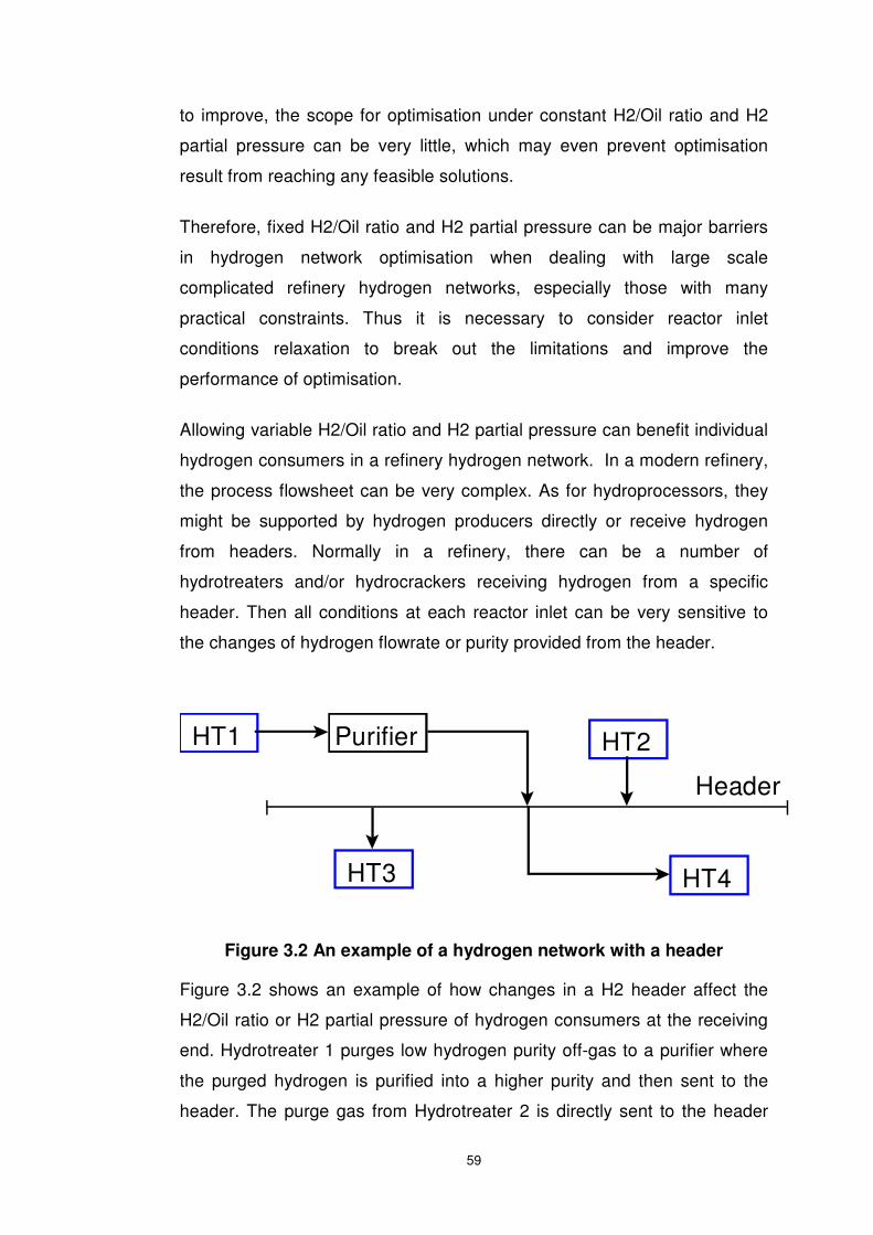
59
to improve, the scope for optimisation under constant H2/Oil ratio and H2
partial pressure can be very little, which may even prevent optimisation
result from reaching any feasible solutions.
Therefore, fixed H2/Oil ratio and H2 partial pressure can be major barriers
in hydrogen network optimisation when dealing with large scale
complicated refinery hydrogen networks, especially those with many
practical constraints. Thus it is necessary to consider reactor inlet
conditions relaxation to break out the limitations and improve the
performance of optimisation.
Allowing variable H2/Oil ratio and H2 partial pressure can benefit individual
hydrogen consumers in a refinery hydrogen network. In a modern refinery,
the process flowsheet can be very complex. As for hydroprocessors, they
might be supported by hydrogen producers directly or receive hydrogen
from headers. Normally in a refinery, there can be a number of
hydrotreaters and/or hydrocrackers receiving hydrogen from a specific
header. Then all conditions at each reactor inlet can be very sensitive to
the changes of hydrogen flowrate or purity provided from the header.
HT1 Purifier
HT4
Header
HT2
HT3
Figure 3.2 An example of a hydrogen network with a header
Figure 3.2 shows an example of how changes in a H2 header affect the
H2/Oil ratio or H2 partial pressure of hydrogen consumers at the receiving
end. Hydrotreater 1 purges low hydrogen purity off-gas to a purifier where
the purged hydrogen is purified into a higher purity and then sent to the
header. The purge gas from Hydrotreater 2 is directly sent to the header
60
without any purification. Then the hydrogen of the header is provided to
Hydrotreater 3 and Hydrotreater 4. As the header hydrogen is the only
source for Hydrotreaters 3 and 4, the hydrogen partial pressures of
hydrotreater 3 and 4 will be determined only by the hydrogen purity of the
header. It is clear that the hydrogen partial pressure will be affected by the
purity change of the header. For example, if we improve the purification
performance of the header, the purity of the header will rise, and
consequently result in improved hydrogen partial pressure at the inlet of the
reactors of Hydrotreaters 3 and 4. However, all these benefits can not
happen if we do not allow H2/Oil ratio or H2 partial pressure to vary. If we
stick to fixed H2/Oil ratio and H2 partial pressure, there will be no flexibility
for HT3 and HT4, and the improved purification would be of no benefit at all.
Nevertheless, what if we relax the H2/Oil ratio and hydrogen partial
pressure? For the same hydrogen network example in Figure 3.2, if H2/Oil
ratio and H2 partial pressure of Hydrotreaters 3 and 4 are allowed to vary,
the change of the hydrogen purity in the header can provide extra potential
in hydrogen network management.
3.2 Sensitivity Analysis of Variable H2/Oil Ratio and H2
Partial Pressure on Hydroprocessor Operation
Since the benefits of allowing H2/Oil ratio and H2 partial pressure to vary is
obvious, it is important to integrate the idea into the modelling of hydrogen
networks. Therefore the first step is to investigate how small changes in
H2/Oil ratio and H2 partial pressure affect other operating conditions in a
hydrogen processor.
3.2.1 H2/Oil Ratio and H2 Partial Pressure vs Product Yield
Considering the operation of a hydroprocessor, the H2/Oil ratio and H2
partial pressure can be very important parameters. Previous researches
(Han, 2001) investigated the variable H2/Oil ratio and H2 partial pressure’s

61
effects on product yield.
The experiment result regarding product yield under different H2 partial
pressure for a hydrocracker was proposed by (Han, 2001). The feedstock
used in his experiment is vacuum gas oil (VGO) with boiling range 340–
530°C. Sulphur content is 2.3wt% while nitrogen content is 0.08wt%. The
experiment of the hydrocracker is performed under two different reaction
partial pressure levels: 14MPa and 7MPa representing high pressure and
intermediate pressure conditions respectively.
Table 3.1 Product yield under different H2 partial pressure
H2 partial pressure 112 (bar) 49 (bar)
Product yield wt% wt%
H2S+NH3 2.5 2.5
C1+C2 0.5 0.5
C3+C4 3.8 4.1
Naphtha 19.0 20.0
Jet fuel 34.8 34.0
Diesel 41.7 40.6
(Han, 2001)
Table 3.1 shows the experiment results of the comparison of product yield
under different H2 partial pressure for a hydrocracker. As can be seen from
the table the gas product is exactly the same under different pressure
levels and while liquid product varies only slightly.
Another investigation regarding H2 partial pressure’s effects in a
hydrocracker was done by UOP Company (Han, 2001). The feed stock is
chosen as two different pressure levels: 56bar and 91bar. The comparison
includes not only the product yield under different pressure levels, but also
the product yield at early and late stage of the operation under the same
pressure level.

62
Table 3.2 Product yield under different reaction pressure
H2 partial pressure 91 (bar) 56 (bar) 91(bar)
Operating time (Month)
1 3 8
Product yield wt% wt% wt%
C1-C4 1.2 1.4 1.5
C5-C6 1.1 1.0 1.0
C7-166°C 1.9 2.0 2.0
166-249°C 6.4 6.0 6.2
249-343°C 18.4 18.6 18.5
>343°C 69.2 69.1 69.2
(Han, 2001)
The results and data comparison shown in Table 3.2 show the product
yield changes under different reaction pressure. Obviously the H2 partial
pressure would vary under different reaction pressure, which is determined
by reaction pressure and H2 purity (H2 partial pressure = Reaction
pressure * H2 purity). The results show that the product yield is almost the
same under high and low pressure. On the other hand, under the same
pressure, the product yield after 8 months operating is still the same as that
of the first month of operation.
The proposed simulations used different feed stock and operating
conditions to test the relative product yield changes for a hydrocracker. All
the results show that the product yield is not changed significantly under
different pressure levels. Therefore, it is reasonable to assume that product
yields of a hydroprocessor will not be affected by marginal changes of its
H2 partial pressure.
3.2.2 H2/Oil Ratio and H2 Partial Pressure vs H2
Recycle/Purge
In order to verify the significance of variable H2/Oil ratio and H2 partial
pressure, the effects on recycle and purge streams in a hydrogen
consumer from varying H2/Oil ratio and H2 partial pressure also need to be

63
investigated. Through monitoring flowrate and purity changes in these two
streams, the relevant effects of changing reactor inlet conditions on reactor
outlet can be monitored.
H P FLASH
H2 Make - Up
Liquid Feed
Liquid Product
Purge
Recycle
Hydrocracker
Reactor
Figure 3.3 The hydrocracker model for verification
A simplified hydrogen consumer (hydrocracker) model (Alves, 1999) is set
up with variable H2/Oil ratio and H2 partial pressure consideration by giving
small changes to the hydrogen flowrate and purity at the inlet of the reactor
model in the mathematical formulation.
On the basis of the hydrocracker model shown in Figure 3.3, a number of
simulation scenarios have been run. Firstly, the values of H2 partial
pressure is changed both upwards and downwards in a small range, whilst
the H2/Oil ratio is maintained the same as the base case.
The simulation with variable H2 partial pressure and constant H2/Oil ratio is
configured under the following conditions:
• Base case conditions: H2/Oil ratio (1544.3 Nm3/m3), H2 partial
pressure (107.6 bar)
• Constant H2/Oil ratio: 1544.3341 Nm3/m3
• Varying H2 partial pressure range: 107.1 – 108.1 bar
The hydrocracker model is created In ASPEN PLUS as shown in Figure
3.4.

64
Figure 3.4 The hydrocracker model for verification in ASPEN PLUS
The way H2 purity is changed at the reactor inlet is to change the hydrogen
purity in the make-up stream. According to the flowsheet shown in Figure
3.4, when the hydrogen purity in the make-up varies, the hydrogen purity at
the reactor inlet will consequently change, leading to variations of the H2
partial pressure.
Table 3.3 Variable H2/Oil ratio and H2 partial pressure strategy
simulation scenarios
H2 PP (bar)
Er% H2/Oil Ratio
(Nm3/m3) Er%
Recycle/ Purge
H2 Purity (Vol%)
Er% Recycle (Nm3/h)
Er% Purge
(Nm3/h) Er%
107.0812 0.4969 1544.3341 0 81.4354 0.3977 127072 0 56.6780 1.2637
107.2951 0.2981 1544.3341 0 81.556 0.2502 127072 0 56.9740 0.7480
107.4555 0.1490 1544.3341 0 81.6756 0.1040 127072 0 57.2067 0.3426
107.6159 0 1544.3341 0 81.7606 0 127072 0 57.4034 0.0000
107.7763 0.1490 1544.3341 0 81.8499 0.1092 127072 0 57.5770 0.3025
107.9367 0.2981 1544.3341 0 81.9212 0.1964 127072 0 57.8077 0.7043
108.0971 0.4471 1544.3341 0 82.011 0.3063 127072 0 58.0376 1.1048
Table 3.3 shows the simulation results of 7 scenarios and each of them are
operated at a different pressure level. The shaded row in Table 3.3 is
shown in the middle of the table as the base case. The detailed data for
H2/Oil ratio and H2 partial pressure at each scenario and the deviations

65
between them can be found from the table. The flowrate and purity
deviations among these scenarios are also shown.
Figure 3.5 The recycle/purge purity vs H2 partial pressure
In order to analyze the changing trends of recycle and purge streams
according to the changes of the H2 partial pressure, all the detailed data in
Table 3.3 have been plotted into diagrams from Figure 3.5 to Figure 3.7.
Since the recycle and the purge streams both come from the high pressure
flash vapour, they have the same hydrogen purity. Hence, the
recycle/purge H2 purity is plotted against the varying H2 partial pressure in
Figure 3.5. As can be seen from the figure, as the H2 partial pressure
increases, the recycle/purge H2 purity increases slightly. The purity is
raised from 81.4354 vol% at a H2 partial pressure 107.0812 bar (lowest
point) to 82.011 vol% at a H2 partial pressure 108.0971 bar (highest point).
With a 0.94% increase of H2 partial pressure in total, the recycle/purge
purity has only increased by 0.71%.

*All points show the same flowrate value. No error between each other.
66
Figure 3.6 The purge flowrate vs H2 partial pressure
Figure 3.6 shows the relationship between the purge flowrate and the H2
partial pressure. As the figure shows, the purge flowrate is increased from
56.6780Nm3 to 58.0376Nm3 as a result of the increase of H2 partial
pressure from 107.0812 bar to 108.0971 bar. The flowrate of the purge
stream is slightly increased by about 1.4Nm3 in total resulting from the
0.94% increase of H2 partial pressure.
Figure 3.7 The recycle flowrate vs H2 partial pressure*

67
On the other hand, as shown in Figure 3.7, the flowrate of the recycle
stream shows no change during the change of the H2 partial pressure.
Another investigation is carried out with H2/Oil ratio and H2 partial pressure
both varying. The simulation with both variable H2 partial pressure and
H2/Oil ratio is configured under the following situations:
• Base case conditions: H2/Oil ratio (1544.3 Nm3/m3), H2 partial
pressure (107.6 bar)
• Varying H2/Oil ratio range: 1536.66 – 1551.24 Nm3/m3
• Varying H2 partial pressure range: 107.1 – 108.1 bar
Table 3.4 Variable H2/Oil ratio and H2 partial pressure strategy
verification simulation scenarios
H2 PP (bar)
Er% H2/Oil Ratio
(Nm3/m3) Er%
Recycle/ Purge
H2 Purity (Vol%)
Er% Recycle (Nm3/h)
Er% Purge
(Nm3/h) Er%
107.08 0.50 1536.66 0.49 81.03 0.88 127072 0 56.29 1.92
107.24 0.35 1538.96 0.34 81.21 0.67 127072 0 56.62 1.35
107.40 0.20 1541.26 0.19 81.44 0.38 127072 0 56.95 0.78
107.62 0 1544.33 0 81.76 0.00 127072 0 57.40 0
107.78 0.15 1546.63 0.14 81.99 0.28 127072 0 57.74 0.59
107.94 0.29 1548.93 0.29 82.23 0.57 127072 0 58.08 1.19
108.10 0.45 1551.23 0.44 82.38 0.76 127072 0 58.43 1.80
The detailed data of the simulation results is shown in Table 3.4. Similarly,
the numbers have been plotted into Figures 3.8 to 3.10 to show effects on
the downstream flows from variable H2/Oil ratio and H2 partial pressure.
According to Figure 3.8, the recycle/purge H2 purity has increased only
slightly during the increase of H2/Oil ratio and H2 partial pressure. The
recycle/purge H2 purity rises from 80.9761 vol% at a H2 partial pressure
107.0812 bar and a H2/Oil ratio 1536.662 Nm3/m3 (lowest point) to 82.467
vol% at a H2 partial pressure 108.0971 bar and a H2/Oil ratio 1551.237
Nm3/m3 (highest point). The recycle/purge H2 purity has only increased by
1.5%.
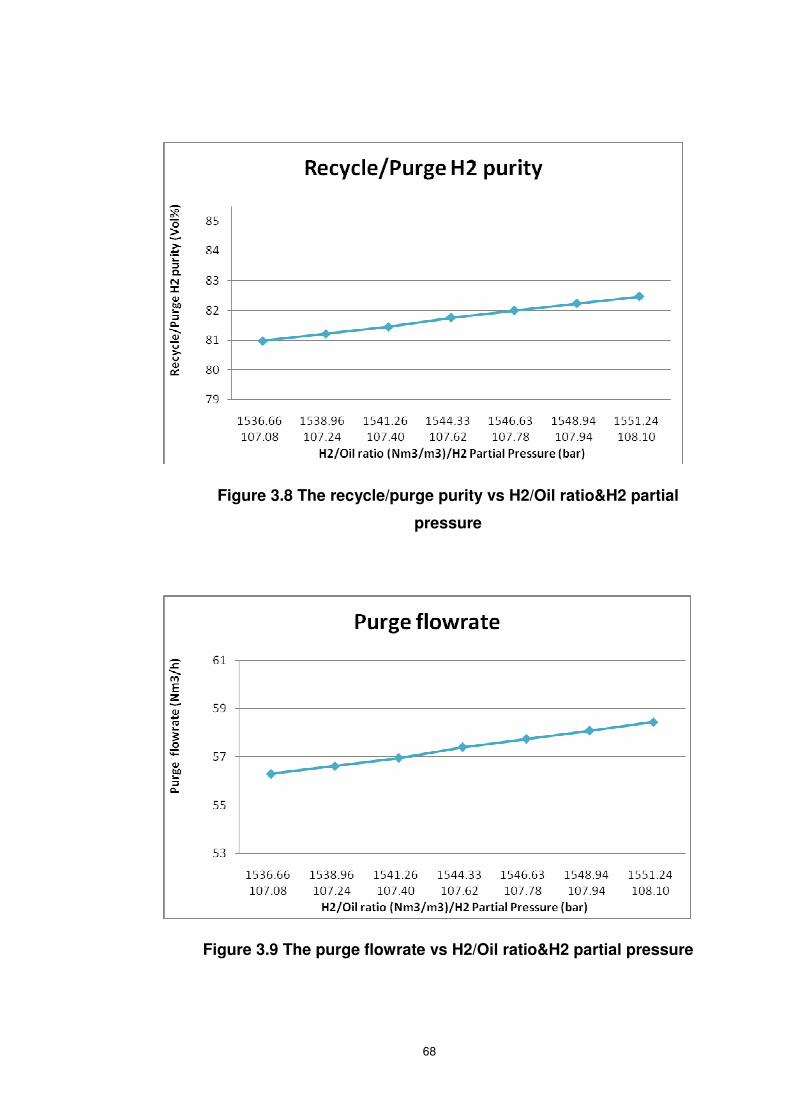
68
Figure 3.8 The recycle/purge purity vs H2/Oil ratio&H2 partial
pressure
Figure 3.9 The purge flowrate vs H2/Oil ratio&H2 partial pressure

69
Figure 3.10 The recycle flowrate vs H2/Oil ratio&H2 partial
pressure
Figure 3.9 shows how the purge flowrate varied according to the varied
H2/Oil ratio and H2 partial pressure. During the increase of reactor inlet
conditions, the purge stream flowrate has increased from 56.3 Nm3/h to
58.4 Nm3/h, indicating only 2Nm3/h of purge flowrate increase.
As can be seen from Figure 3.10, although the H2/Oil ratio and H2 partial
pressure have been increased by certain amount, the recycle flowrate can
be maintained the same as the base case.
3.2.3 Conclusions from the Sensitivity Analysis
From the sensitivity analysis, it is clear that when H2 partial pressure
changes marginally, the recycle flowrate can maintain constant. For the
purge flowrate and purge/recycle purity, there are only slight changes.
To simplify the model building of hydroprocessors, it is reasonable to
assume that marginal variation in H2 partial pressure does not affect the
performance of a hydrogen consumer in terms of product yields and
operating conditions such as recycle and purge flows/purity. It is important

70
to point out that in practice, such an assumption has to be verified by
relevant process engineers, and different criteria may be applied to
individual process units.
3.3 Improved Hydrogen Network Formulation and
Optimisation Methodology
The relaxation of reactor inlet conditions requires new mathematical
formulation of hydrogen networks. Both automated hydrogen network
design (Liu, 2002) and multi-component hydrogen network optimisation
(Zhang et al., 2008) methods are set up with fixed H2/Oil ratio and H2
partial pressure by fixing H2 flowrate and purity at hydrogen sinks. In this
work variable H2/Oil ratio and H2 partial pressure are applied into the new
formulation to provide extra freedom for each hydrogen consumer in a
hydrogen network.
3.3.1 Mass Balance of Hydrogen Producers
The mass balance of hydrogen producers represents the hydrogen
transportation from hydrogen producers to hydrogen consumers, hydrogen
headers, and purifiers:
jFIFIFIFIn k kinij jii ∀++= ∑ ∑∑ ,,, (3.1)
Where FI represents the total flowrate of hydrogen producers, the
subscripts i, j, n and k represent hydrogen producers, consumers, headers
and purifiers respectively. In reality, the throughput of a hydrogen producer
is normally constrained due to practical limitations, and these limits can be
formulated as:
jFIFIFI iii ∀≤≤ maxmin (3.2)
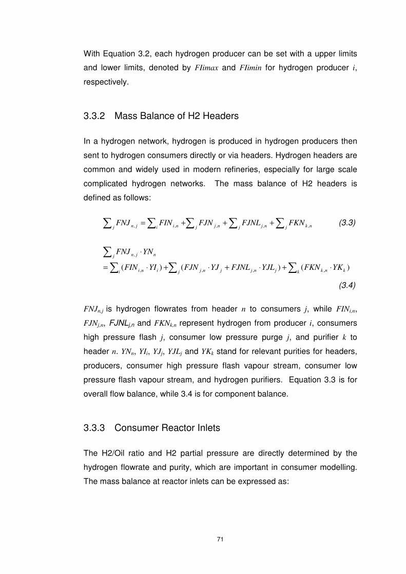
71
With Equation 3.2, each hydrogen producer can be set with a upper limits
and lower limits, denoted by FIimax and FIimin for hydrogen producer i,
respectively.
3.3.2 Mass Balance of H2 Headers
In a hydrogen network, hydrogen is produced in hydrogen producers then
sent to hydrogen consumers directly or via headers. Hydrogen headers are
common and widely used in modern refineries, especially for large scale
complicated hydrogen networks. The mass balance of H2 headers is
defined as follows:
∑ ∑∑∑∑ +++=j j nknjj nji nij jn FKNFJNLFJNFINFNJ ,,,,, (3.3)
)()()( ,,,,
,
kk nkj jnjjnji ini
j njn
YKFKNYJLFJNLYJFJNYIFIN
YNFNJ
⋅+⋅+⋅+⋅=
⋅
∑∑∑∑
(3.4)
FNJn,j is hydrogen flowrates from header n to consumers j, while FINi,n,
FJNj,n, FJNLj,n and FKNk,n represent hydrogen from producer i, consumers
high pressure flash j, consumer low pressure purge j, and purifier k to
header n. YNn, YIi, YJj, YJLj and YKk stand for relevant purities for headers,
producers, consumer high pressure flash vapour stream, consumer low
pressure flash vapour stream, and hydrogen purifiers. Equation 3.3 is for
overall flow balance, while 3.4 is for component balance.
3.3.3 Consumer Reactor Inlets
The H2/Oil ratio and H2 partial pressure are directly determined by the
hydrogen flowrate and purity, which are important in consumer modelling.
The mass balance at reactor inlets can be expressed as:

72
∑∑∑∑∑ ++++=n jnk jkjjj jji jij j FNJFKJFJLFJFIJFC ,,,11 ,1, )( (3.5)
)(
)()()(
,
,1 1,11,1,
nn jn
kk jkj jjjjjji iji
j jj
YNFNJ
YKFKJYJLFJLYJFJYIFIJ
YCFC
⋅+
⋅+⋅+⋅+⋅=
⋅
∑∑∑∑
∑
(3.6)
Where FCj denotes the total reactor inlet flowrate of consumer j. Subscript
j1 is introduced as an alias of j so that flow from j1 to j or j to j1 can cover
recycle and hydrogen transportation between different consumers. FIJi,j,
FKJk,j and FNJn,j represent flowrate from hydrogen producer i, purifier k and
header n to consumer j. FJj1,j and FJLj1,j are used to represent the flowrates
of the vapour stream from high pressure flash and low pressure flash.
When j1 equals to j, the flowrate is the internal recycle of the consumer j.
When j1 is different from j, they are representing different consumers, so
the flow between them would be the hydrogen transportation from a
hydrogen consumer’s high or low pressure flash to another consumer. YCj
stands for hydrogen purities at the reactor inlets of consumer j, while YIi,
YJj1, YJLj1, YKk, and YNn stand for hydrogen purities of hydrogen producer i,
vapour stream from high pressure flash of consumer j, vapour stream from
low pressure flash of consumer j, purifier k and header n, respectively.
With Equations 3.3 and 3.4 the mass balance and hydrogen balance are
calculated. However the reactor inlet modelling is still incomplete without
limits on H2/Oil ratio and H2 partial pressure. In the existing hydrogen
optimisation methodology (Zhang et al., 2008), the H2/Oil ratio and H2
partial pressure are set as constants through fixing mass flowrates and
pure hydrogen flow at inlets of reactors. Considering variable H2/Oil ratio
and H2 partial pressure at reactor inlets, the mass flowrates and pure
hydrogen at reactor inlets should be given certain freedom to vary. As a
result, an upper limit parameter and a lower limit parameter are introduced
to enable the varying range for variable reactor inlet conditions. On the
basis of Equations 3.4 and 3.5, the reactor inlet conditions relaxation
Equation 3.6 and 3.7 are introduced:

73
jFCFCFC jjj ∀≤≤ maxmin (3.7)
jYCFCYCFCYCFC jjjjjj ∀⋅≤⋅≤⋅ maxmaxminmin (3.8)
Parameter FCjmax and FCjmin indicate the upper and lower flowrate limits at
the reactor inlet of consumer j. YCjmax and YCjmin indicate the relevant
hydrogen purity. With the introduced upper bounds and lower bounds, the
total flowrate of reactor inlets (FCj) and the pure hydrogen going into
reactor inlets ( jj YCFC ⋅ ) are allowed certain space to vary instead of fixing
them at a constant level. In this way, H2/Oil ratio and H2 partial pressure
constraints are relaxed.
Apart from reactor inlets, the make-up hydrogen stream in a hydrogen
consumer may be under limits as well due to practical restrictions.
jjjj FMUMAXFJFC ≤− , (3.9)
FJj,j denotes internal recycle flowrate of consumer j. As an upper limit
parameter, FMUMAXj is set as the maximum value for hydrogen make-up
stream flowrate.
3.3.4 Consumer Flash Calculation
The consumer flash calculation is simplified and expressed by hydrogen
balance at the hydrogen consumer outlets.
For high pressure flash hydrogen balance:
∑ ∑ ∑ +++=1 ,,1,j k n jnjkjjjj FJPFJNFJKFJFJ (3.10)
FJj represents the total flowrate of the vapour stream from high pressure
flash of consumer j, while FJj,j1, FJKj,k and FJNj,n represents hydrogen
transportation from this high pressure flash to other consumers or recycle,
purifiers and headers. FJPj represents high pressure purge gas sent to the
site fuel.

74
For low pressure flash hydrogen balance:
jj k n njkjjjj FJLPFJLNFJLKFJLFJL +++=∑ ∑ ∑1 ,,1, (3.11)
FJLj represents the total flowrate of the vapour stream from low pressure
flash of consumer j, while FJLj,j1, FJLKj,k and FJLNj,n represent hydrogen
transportation from this low pressure flash to other consumers or recycle,
purifiers and headers. FJLPj represents low pressure purge gas sent to the
site fuel.
3.3.5 Mass Balance of Purifiers
In a hydrogen network, hydrogen purifiers are used for hydrogen recovery
and re-use. Normally a hydrogen purifier intakes tail gas from hydrogen
consumers and purifies it then sends it back to consumers. The mass
balance of hydrogen purifiers in a hydrogen network can be expressed by
hydrogen balance between inlets and outlets of purifiers.
[ ]( )
kn nkj jk
ki ikij jkjjkj
YKFKNFKJ
RECPYIFIKYJLFJLKYJFJK
⋅+=
⋅⋅+⋅+⋅
∑∑∑∑
,,
,,, )()( (3.12)
FJKj,k, FJLKj,k and FIKi,k denote the hydrogen flowrate from high pressure
flash of consumer j, low pressure flash of consumer j and producer i
respectively, while YJj, YJLj and YIi denote their relevant purity. FKJk,j and
FKNk,n express the hydrogen flowrate from purifier k to consumer j or
header n. Parameter RECPk is used as the rate of hydrogen recovery for
purifier k.
The throughput of a hydrogen purifier must have an upper limit in hydrogen
network design.
kn nkj jk FKMAXFKNFKJ ≤+∑∑ ,, (3.13)
FKJk,j stands for the flowrate from purifier k to consumer j and FKNk,n

75
stands for the flowrate from purifier k to header n. The summation of these
flowrates is the total flowrate at the outlet of purifier k and this value should
always not be higher than the maximum limits of the purifier k set by
parameter FKMAXk.
3.3.6 Power Consumption of Compressors
In a hydrogen network, there are make-up compressors to increase
pressure of hydrogen when it is needed.
For make-up compressors:
∑ ∑∑ ∑ ∑ ++++⋅⋅=1 1 ,1,1,,, )(
j j jjjji k n jnjkjijfj FJLFJFNJFKJFIJPCMUECMU
( jj ≠1 for FJ)
(3.14)
CMUj represents total power consumption for make-up hydrogen
compression of consumer j. Two parameters, Ef and PCMUj, are defined
as the efficiency parameter and the power rate (unit compression power
duty). When jj ≠1 , the flowrate between j1 and j would be between
different consumers, where a make-up hydrogen compressor may be
needed.
For recycle compressors:
jjjfj FJPCREECRE ,⋅⋅= (3.15)
Similarly, CREj denotes total power consumption for the recycle
compressor of consumer j. Ef and PCREj are for efficiency and power rate
of the recycle compressor of consumer j. FIj,j is used to represent the
flowrate from consumer j to itselt, which is actually the recycle flowrate for
consumer j.
3.3.7 Summary of Binary H2 Network Modelling
76
With all the proposed equations, an overall binary hydrogen network model
is completed. On the basis of the hydrogen network model, the design and
optimisation strategy for binary hydrogen network can be developed. For
an optimisation problem, a few definitions need to be made beforehand,
including:
� Variables
The variables of binary hydrogen network optimisation problems mainly
include the stream flowrates and purities around a hydrogen network, for
example the flowrate and purity for hydrogen from producers to consumers
or from headers or purifiers to consumers. It also includes the flowrates
and purities of hydrogen between consumers. Also there are variables for
power calculation of compressors.
� Parameters
Many parameters are involved in the formulation equations such as
process pressures, hydrogen production unit prices, and upper bound and
lower bound values for reactor inlet conditions and hydrogen production for
producers, maximum limits for make-up hydrogen of each hydrogen
consumer as well as the throughput of purifiers. In addition, for
compressors the power rate and efficiency are also set in order to calculate
the compression power cost.
� Constraints
The constraints for binary hydrogen network optimisation problems are
mainly the mass balance around the network between hydrogen sources
and sinks. As expressed with Equation 3.1 to Equation 3.15, the mass
balances for hydrogen producers, consumers, headers and purifiers have
been formulated. All these equations are to be used as the problem
constraints during optimisation.
� Objective function

77
In this work the optimisation objective can be set as the minimum total
operating cost. Therefore on the basis of Equations 3.1 - 3.15, the
optimisation objective function can be expressed as:
)Pr( 2 ueFuelGasValtUtilityCosiceUnitFIMINOBJi Hi −+⋅= ∑ (3.16)
As stated in Equation 3.16, the total operating cost includes hydrogen
production cost, utility cost and fuel gas value. The production cost is
calculated using unit price of hydrogen production times the total
production flowrate. On the other hand, the fuel gas value calculation would
be based on the heating values of the components contained in the fuel
gas. By minimising the result of summation of hydrogen production and
utility cost minus the fuel gas value, the total operating cost of a hydrogen
network can be minimised.
As discussed before, the improvements of this formulation is mainly the
inclusion of variable H2/Oil ratio and H2 partial pressure. In this way, the
overall hydrogen network is more flexible than before, which may brings
more and better design ideas or solutions in the optimisation.
3.4 Optimisation Methodology
For the optimisation methodology, it is important to point out the key
conditions for the assumptions before getting into it.
3.4.1 Key Assumptions
There are two main assumptions in this binary hydrogen network
optimisation methodology:
• Binary component based hydrogen network
• Marginal changes in H2/Oil ratio and H2 partial pressure not
affecting hydrogen consumer operation

78
A binary hydrogen network means that, for each stream in the network, all
the other component apart from hydrogen is lumped as one impurity
component for example CH4. In this case, the mass balance around the
network is actually the mass balance of hydrogen. The binary system is
applied in order to simplify the optimisation calculation and ease the
convergence. Without considering the mass balance of all components in a
stream, the amount of computation effort can be dramatically reduced to
improve the calculation efficiency.
The other assumption is allowing marginal changes in H2/Oil ratio and H2
partial pressure for a hydrogen consumer. The main reason of this
assumption is to provide all reactor inlets in the network with extra degrees
of freedom in hydrogen network design. As in both Liu (2002) and Zhang
(et al., 2008)’s methods, the reactor inlet conditions are strictly fixed as
constants, making it easier to justify hydrogen management decisions.
They also reduce the system design flexibility, especially for large scale
complicated hydrogen networks that under a number of practical
constraints. For those specific hydrogen networks, the space for
optimisation can be very limited, and if reactor inlets are still strictly fixed,
the hydrogen network optimisation problem can be over-constrained
leading to difficulties in solving problems or even no solutions for the
problem. Due to these concerns, the variable H2/Oil ratio and H2 partial
pressure strategy have been introduced. With Equations 3.7 and 3.8, the
hydrogen flowrate and purity at the reactor inlet is allowed in a range to
vary. The parameters for upper and lower limits will be carefully set to
make sure the feasibility of the reactor and the balance of the hydrogen
consumer model.
3.4.2 Optimisation Framework
Based on the proposed binary hydrogen network modelling, the
optimisation framework for the binary hydrogen network optimisation is
shown in Figure 3.11.

79
Figure 3.11 Binary hydrogen network optimisation framework
The optimisation methodology can be summarised into a few stages. At the
beginning the hydrogen pinch method is used to get hydrogen composite
curves and surplus curve to scope for potentials of the network. If there is
no potentials found, investigation will be terminated or directed to problem
redefinition. The binary hydrogen network optimisation is formulated as a
non-linear problem. When an optimisation solution is obtained, it will then
be simulated and compared with optimisation results to check deviations
between them for feasibility. If the deviation criterion is not met, the base
case will be updated with the results and perform the optimisation again
from the beginning until the convergence criterion is finally satisfied.
The new mathematical formulation with considerations of variable H2/Oil
ratio and H2 partial pressure can be applied with the following steps:
• Set up model for the H2 network
Start
Hydrogen pinch analysis for base case
NLP Optimisation with variable H2/Oil ratio and H2 partial pressure considerations
Simulation to check the feasibility of results
Scope for Improvements
Optimal solution
∆ Obj ≤ έ No
Yes
Update Base case
Stop investigation or redefine problem
No
Check deviation between optimisation and simulation

80
• Initially fix the configuration
• Optimise the system allowing H2/Oil ratio and H2 partial pressure to
vary between limits
• In this case only increase in H2/Oil ratio and H2 partial pressure is
allowed
In this way a hydrogen network can be incorporated with flexible reactor
inlet conditions for each hydrogen consumer, which will open up the
degrees of freedom for the network, and reach better optimisation solutions.
The variable H2/Oil ratio and H2 partial pressure can be counter-intuitive
especially for hydrogen networks under many practical constraints, which
will be shown in the forthcoming case study.
3.5 Case study
The case study for the hydrogen network optimisation with variable H2/Oil
ratio and H2 partial pressure considerations is taken from an industrial
project. A refinery undertakes a retrofit design project that will increase its
crude oil through put from 1.35MT/year to 1.8MT/year, which brings in new
processes so that the overall hydrogen requirement for the refinery will be
hugely increased. As a result, the hydrogen network management is then
required to optimise the hydrogen utilization in order to save H2 utility or
operating cost of hydrogen consumers or purifiers.
The hydrogen network to be optimised is located within the refinery with a
number of hydrogen consumers and producers as well as relatively
supporting processes such as purifiers. On the other hand, an ethylene
plant also produces hydrogen as a by-product which is sent to the refinery
as a hydrogen source. So this part of hydrogen will be considered in the
hydrogen network optimisation as well.
3.5.1 Software Tool
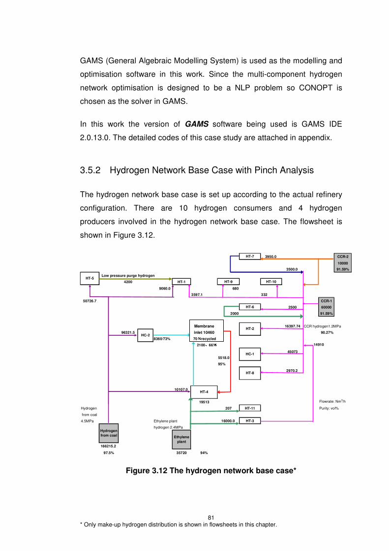
* Only make-up hydrogen distribution is shown in flowsheets in this chapter.
81
GAMS (General Algebraic Modelling System) is used as the modelling and
optimisation software in this work. Since the multi-component hydrogen
network optimisation is designed to be a NLP problem so CONOPT is
chosen as the solver in GAMS.
In this work the version of GAMS software being used is GAMS IDE
2.0.13.0. The detailed codes of this case study are attached in appendix.
3.5.2 Hydrogen Network Base Case with Pinch Analysis
The hydrogen network base case is set up according to the actual refinery
configuration. There are 10 hydrogen consumers and 4 hydrogen
producers involved in the hydrogen network base case. The flowsheet is
shown in Figure 3.12.
HT-7 3950.0 CCR-2
10000
3500.0 91.59%
Low pressure purge hydrogen
4200 HT-1 HT-9 HT-10
9060.0 680
3597.1 332
50726.7 CCR-1
HT-6 2500 60000
2000 91.59%
Membrane 16397.74 CCR hydrogen1.2MPa
96321.5 inlet 10460 90.27%
8360/73% 70%%%%recycled
2100,,,,66%%%%45073
5518.0
95%
2970.2
10107.0
19513 Flowrate: Nm3/h
Hydrogen 207 HT-11 Purity: vol%
from coal
4.5MPa Ethylene plant 16000.0 HT-3
hydrogen 2.4MPa
166215.2
97.5% 35720 94%
Hydrogen
from coal
HT-5
HC-2
Ethylene
plant
HT-2
HC-1
HT-8
HT-4
14910
Figure 3.12 The hydrogen network base case*

82
The hydrogen producers and hydrogen consumers involved in the base
case can be summarised as:
• Hydrogen producers: catalytic reformer 1 (CCR-1), catalytic reformer
2 (CCR-2), ethylene plant, and hydrogen from coal gasification
• Hydrogen consumers: HT-1, HT-2, HT-3, HT-4, HT-5, HT-6, HT-7,
HT-8, HT-9, HT-10, HT-11
• Hydrogen purifiers: Membrane
The entire hydrogen network contains of three hydrogen distribution
headers under different pressure levels. CCR hydrogen is with 1.2MPa
while the ethylene plant and the coal-based hydrogen plant are with
relatively higher 2.4MPa and 4.5MPa respectively. From the flowrate point
of view, the hydrogen from coal accounts for the biggest portion of
hydrogen supply at 166215 Nm3 per hour, which is more than the total of all
other hydrogen sources including hydrogen from the ethylene plant, CCR-1
and CCR-2. Moreover, the purity of hydrogen generated from the coal-
hydrogen plant is 97.5%, also higher than 94% of the ethylene plant and
91.59% of CCR-1 and CCR-2.
The utilisation strategy of hydrogen resources has been set under the
following considerations:
• All reactor inlet conditions of hydroprocessing units should be no
lower than values of the base case.
• 4.5MPa pressure hydrogen is mainly used for process with higher
hydrogen partial pressure.
• 2.4MPa pressure hydrogen including membrane purified hydrogen
and ethylene hydrogen supports HT-3, HT-4 and HT-11.
• 1.2MPa pressure hydrogen only consisting of two CCR units with
purity 91.59% and total 70000Nm3/h flowrate supplying hydrogen to
HC-1, HT-1, HT-2, HT-7, HT-8, HT-9, HT-10.

* Hydrogen listed in tables for reactor inlets in this chapter includes both make-up and recycle hydrogen.
83
Table 3.5 Reactor inlet conditions for the base case*
Process Hydrogen purity v% Hydrogen flowrate
Nm3/h Pure hydrogen flowrate
Nm3/h
HC-1 84.22 165346 139254
HC-2 94.45 503921 475953
HT-1 87.02 123102 107123
HT-2 84.46 126554 107261
HT-3 92.00 16000 14720
HT-4 80.39 158572 127803
HT-5 93.91 409977 384998
HT-6 91.00 2484 2260
HT-7 91.00 3950 3600
HT-8 87.03 11732 10210
Table 3.5 shows all detailed data for reactor inlet conditions of all hydrogen
consumers in the hydrogen network, including hydrotreaters and
hydrocrackers. All the hydrogen purity and flowrate as well as net hydrogen
flowrate are shown in the table. These values are listed not only for
checking the reactor inlet conditions of the base case, but also for
comparison with optimisation solutions.
Hydrogen flowrate: Nm3/h
Figure 3.13 Hydrogen surplus curve for the base case
Hyd
rog
en p
urity
: vo
l%

84
Figure 3.13 shows the hydrogen surplus curve for the current base case.
As can be seen from the diagram, on the basis of the existing purification
situation, the present hydrogen plant (mainly hydrogen from coal
gasification) production is already close to the theoretical minimum of the
hydrogen requirement target. The minimum hydrogen target can only be
reached by modifications of pipeline distribution and compressors systems
which are very costly and sometimes unrealistic. However this does not
suggest that there is no saving potential from the hydrogen network. It is
also observed that around 25247Nm3/h hydrogen is not being utilised due
to low purity and sent to site fuel system directly.
In the base case HT-3 is currently adopting a hydrogen once-through
option in order to save compression work from its own recycle compressor.
However, the once-through option of HT-3 reduces the purity of the
ethylene hydrogen source from 94% to 93%. To make sure that the reactor
inlet conditions of all hydrogen consumers are not deteriorated, more
hydrogen production is then required from the coal gasification hydrogen
plant leading to an increased hydrogen utility for the overall hydrogen
network.
In optimisation there are also practical limitations of the hydrogen network
design:
• No continuous high pressure purge is allowed for each hydrogen
consumer
• All hydrogen consumers receive hydrogen from headers
These limitations indicate that if hydrogen purity of the header varies, every
hydrogen consumer fed by the header will be affected simultaneously.
Looking at the purged low purity hydrogen below the pinch, it is straight
forward to think about hydrogen purification and recovery to reduce the
hydrogen requirement. However, considering the discussed practical
constraints, if we purify and re-use hydrogen we will have to change the
reactor inlet conditions unless it has the same purity currently as that of the

85
headers. Therefore, the hydrogen network purification can be improved
only if we allow H2/Oil ratio and H2 partial pressure at reactor inlets to vary.
Figure 3.14 Idea of hydrogen purification below the pinch
To summarise the hydrogen pinch analysis, when operating optimisation or
selecting optimisation solutions, we should be focusing on how to improve
the HT-3 process design or enhance the hydrogen purification, and
increase the rate of hydrogen recovery with variable H2/Oil ratio and H2
partial pressure to extract the potentials of the hydrogen network as much
as possible.
3.5.3 H2 Network Operating Cost
For both new and revamping design, the total network operating cost is a
very important economical factor to consider. In a revamping design, the
operating cost saving can affect the pay back period significantly.
ueFuelGasValtUtilityCosCostproductionHtingCostTotalOpera −+= 2
(3.17)
Normally, the operating cost for a hydrogen network would be the
summation of all utility costs including hydrogen production cost, power,
water and steam costs. Taking into account the fuel gas value, the total net
operating cost for the hydrogen network is the total utility cost minus the
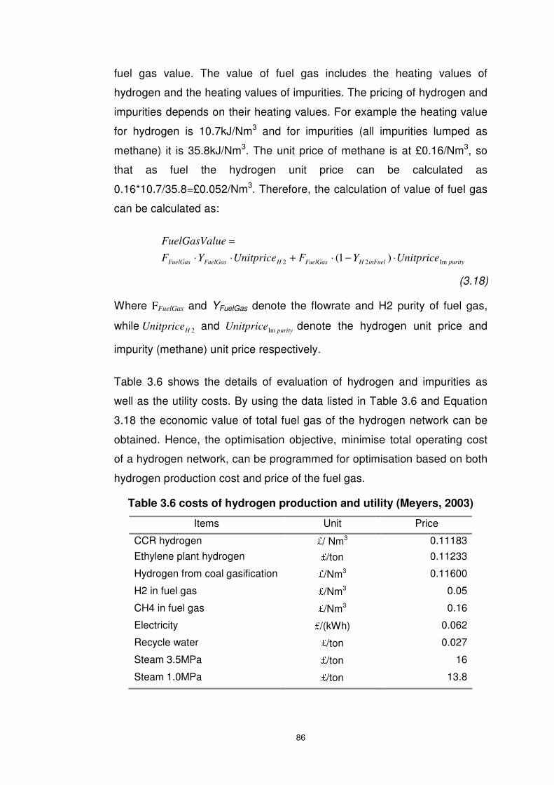
86
fuel gas value. The value of fuel gas includes the heating values of
hydrogen and the heating values of impurities. The pricing of hydrogen and
impurities depends on their heating values. For example the heating value
for hydrogen is 10.7kJ/Nm3 and for impurities (all impurities lumped as
methane) it is 35.8kJ/Nm3. The unit price of methane is at £0.16/Nm3, so
that as fuel the hydrogen unit price can be calculated as
0.16*10.7/35.8=£0.052/Nm3. Therefore, the calculation of value of fuel gas
can be calculated as:
purityinFuelHFuelGasHFuelGasFuelGas UnitpriceYFUnitpriceYF
ueFuelGasVal
Im22 )1( ⋅−⋅+⋅⋅
=
(3.18)
Where FFuelGas and YFuelGas denote the flowrate and H2 purity of fuel gas,
while 2HUnitprice and purityUnitpriceIm denote the hydrogen unit price and
impurity (methane) unit price respectively.
Table 3.6 shows the details of evaluation of hydrogen and impurities as
well as the utility costs. By using the data listed in Table 3.6 and Equation
3.18 the economic value of total fuel gas of the hydrogen network can be
obtained. Hence, the optimisation objective, minimise total operating cost
of a hydrogen network, can be programmed for optimisation based on both
hydrogen production cost and price of the fuel gas.
Table 3.6 costs of hydrogen production and utility (Meyers, 2003)
Items Unit Price
CCR hydrogen £/ Nm3 0.11183
Ethylene plant hydrogen £/ton 0.11233
Hydrogen from coal gasification £/Nm3 0.11600
H2 in fuel gas £/Nm3 0.05
CH4 in fuel gas £/Nm3 0.16
Electricity £/(kWh) 0.062
Recycle water £/ton 0.027
Steam 3.5MPa £/ton 16
Steam 1.0MPa £/ton 13.8

87
3.5.4 Optimisation Solutions Analysis and Comparison
Optimisation solution 1: no new facilities 3950
CCR-2
3500 10000
91.59%
3417 87.30% HT-9
10478.0 391.6 680 332
50726.7 2500 CCR-1
60000
2000 91.59%
Membrane 31628.7 CCR hydrogen
96321.5 inlet 10460 1.2MPa
8360/73% 70%%%%recycled
9060 33047.7
2100 5518.0
66% 95%
2970.2
4540
25293
Hydrogen 1160
from coal Flowrate: Nm3/h
4.5MPa Ethylene plant 207 Purity: vol%
hydrogen 2.4MPa
162066.2
97.5% 35720 94%
HT-7
Ethylene
plant
HT-5 HT-1
HT-4
HT-10
HT-6
HT-8
HT-2
Low pressure Purge hydrogen
HC-2
HT-3
Hydrogen from coal
HC-1
HT-11
Figure 3.15 The optimised hydrogen network of solution 1
The first solution is mainly about the re-configuration of HT-3. As analyzed
in the hydrogen pinch analysis, the once-through operation poses a
question mark on the overall network economics. Therefore in this solution,
the once-through option is compared with the option of complete recycle
operation with no purged hydrogen to improve the hydrogen utilization
efficiency.
The optimised modifications of the hydrogen network structure include:
• Some hydrogen is sent from the ethylene plant to HT-4 so as to
reduce the hydrogen production of coal gasification hydrogen plant
• Some hydrogen from ethylene plant feeds HC-1 as well
• No hydrogen purged from HT-3 to header
Table 3.7 compares the reactor inlet conditions between the base case and
the solution to ensure feasibility.

88
Table 3.7 Reactor inlet conditions comparison for Solution 1
Hydrogen purity v% Hydrogen flowrate
Nm3/h Pure hydrogen flowrate
Nm3/h Process Base case Solution1 Base case Solution1 Base case Solution1
HC-1 84.22 84.22 165346 167462 139254 141036
HC-2 94.45 94.45 503921 503921 475953 475956
HT-1 87.02 87.02 123102 124638 107123 108460
HT-2 84.46 84.54 126554 126875 107261 107261
HT-3 92.00 92.10 16000 16000 14720 14736
HT-4 80.39 80.49 158572 158785 127803 127809
HT-5 93.91 93.91 409977 409977 384998 384998
HT-6 91.00 91.59 2484 2500 2260 2290
HT-7 91.00 91.59 3950 3950 3600 3618
HT-8 87.03 87.03 11732 11732 10210 10210
It is clear that all the hydrogen purities and flowrates in Solutions 1 are
either higher than or equal to those in the base case. The results have
confirmed that the hydrogen consumer reactor inlet conditions are either
maintained or improved with a higher hydrogen purity or flowrate.
With the recycle hydrogen compressor for HT-3 in operation, the required
power has increased by 357.6kWh. However, hydrogen from the coal
gasification requirement and the total amount of purged hydrogen of the
whole network were both reduced by 4,149Nm3/h. Meanwhile, the total
network operating cost was saved by 2.27 million pounds per year.
However, this solution still has an amount of 21,202Nm3 hydrogen being
purged, which could be further recovered, therefore, it should be
investigated further.

89
Optimisation solution 2: additional purification
3950
CCR-2
3500 10000
91.59%
HT9
680 332
4625.0 7790.5
50726.7 2500 CCR-1
60000
96321.5 PSA 2000 91.59%1.2MPa
8360 inlet 31628.7 CCR hydrogen
73% 22540 1.2MPa
Membrane 2921
inlet 10460 33439.2
70% recycled 4353
2100 5518 95% 2970.2
66% 2.4MPa
Hydrogen 1160
from coal Flowrate: Nm3/h
4.5MPa 207 Purity: vol%
Ethylene plant
151673.2 hydrogen 2.4MPa
97.5% 35720 94%
HT6
HT2
HT-8
HT-4
HT-5 HT-1
HT-7
HT10
HT-3
4940/45.5% Membrane
8200/38.5% 1 HC5200/52.2% 3 Diesel HT
4200/87.3% Residue HT
Hydrogen from coal
HT-11
HC-2
HC-1
Ethylene
plant
Figure 3.16 The optimised hydrogen network of solution 2
Considering enhancing the capability of hydrogen recovery, since the
current membrane unit is already on full load, a new purifier needs to be
installed. In this solution a PSA is planned, which will be working along with
the existing membrane. With the capacity of 10000Nm3/h, the PSA can be
used to recover the purged gases from HC-1, HT-2 and the membrane. As
a result, the hydrogen production of hydrogen from coal gasification is
reduced by 14500Nm3 compared with the base case.
The main features of this solution are:
• HT-3 is changed from hydrogen once-through process into complete
H2 recycle process
• Purge gases from HT-5, HC-1, HT-2 and the membrane are sent to
PSA for purification and recovery.
• PSA product to feed HC-1 and HT-1
• HC-1 supported by three hydrogen sources including the ethylene
plant , PSA, and CCR.
• HT-1 fed by hydrogen from the coal gasification and PSA
• HT-4 now receives hydrogen from the ethylene plant only.

90
Table 3.8 Reactor inlet conditions comparison for Solution 2
Hydrogen purity v% Hydrogen flowrate
Nm3/h Pure hydrogen flowrate
Nm3/h Process Base case Solution2 Base case Solution2 Base case Solution2
HC-1 84.22 84.22 165346 166065 139254 139860
HC-2 94.45 94.45 503921 503921 475953 475956
HT-1 87.02 87.26 123102 122767 107123 107124
HT-2 84.46 84.54 126554 126875 107261 107261
HT-3 92.00 92.10 16000 16000 14720 14736
HT-4 80.39 80.41 158572 158954 127803 127809
HT-5 93.91 93.91 409977 409977 384998 384998
HT-6 91.00 91.59 2484 2500 2260 2290
HT-7 91.00 91.59 3950 3950 3600 3618
HT-8 87.03 87.03 11732 11732 10210 10210
Again the hydrogen purities and flowrates for each hydrogen consumer are
compared with the base case to show the how these conditions have been
changed. The overall network purged hydrogen is reduced to about
11,069Nm3/h, leading to considerably reduced network operating cost with
a saving of 6.62 million pounds per year. The investment of the new
installed PSA unit is estimated at 3.2 million pounds. Taking into account
both PSA investment and reduced operating cost, the simple payback
period is only 0.48 year.
Optimisation solution 3: simplified purification scheme
In order to simplify the hydrogen purification system as well as saving
operating cost, this solution considers installing a large scale PSA unit and
meanwhile shutting down the membrane unit. The new PSA is designed at
a capacity of 16,000Nm3/h which is much larger than that of Solution 2, so
that the associated product volume and the capacity of tail gas compressor
would increase. Compared with Solution 2, the modifications made in this
solution are:
• Purge gases from HT-5, HC-1, HT-2, HC-2 and HT-4 are sent to the
new large capacity PSA

91
• HT-4 supported by hydrogen from the ethylene plant and the coal
gasification
• HC-1 fed by PSA and CCR
3950
CCR-2
3500 10000
91.59%
HT-9
680 332
3360.0
50726.7 2500 CCR-1
60000
96321.5 9037.5 2000 91.59%
31628.7 CCR hydrogen
1.2MPa
PSA
1.2MPa 6440 33439.2
inlet
22540
2970.2
1180
34353
Hydrogen 1160
from coal Flowrate: Nm3/h
4.5MPa 207 Purity: vol%
Ethylene plant
151588.2 hydrogen 2.4MPa
97.5% 35720 94%
HT-5 HT-1
HT-7
HT-10
5200/52.2% 3 Diesel HT
HC-2
8200/38.5% 1 HC
HT-6
HT-2
4200/87.3% Residue HT
2100/66% Wax oil HTHC-1
8360/73% 2 HC
HC-4
HT-8
HT-3
Hydrogen from coal
HT-11
Ethylene
plant
Figure 3.17 The optimised hydrogen network of solution 3
Figure 3.17 shows the flowsheet of Solution 3, while Table 3.9 lists all
reactor inlet conditions of hydroprocesses. Similarly, all reactor inlet
conditions are either maintained or improved. So far the results from the
three different optimisation solutions have shown that saving H2 and
improving certain reaction conditions may not be contradictory with each
other.

92
Table 3.9 Reactor inlet conditions comparison for solution 3
Hydrogen purity v% Hydrogen flowrate
Nm3/h Pure hydrogen flowrate
Nm3/h Process Base case Solution3 Base case Solution3 Base case Solution3
HC-1 84.22 84.28 165346 165233 139254 139254
HC-2 94.45 94.45 503921 503921 475953 475956
HT-1 87.02 87.27 123102 122749 107123 107125
HT-2 84.46 84.54 126554 126875 107261 107261
HT-3 92.00 92.10 16000 16000 14720 14736
HT-4 80.39 80.40 158572 158967 127803 127808
HT-5 93.91 93.91 409977 409977 384998 384998
HT-6 91.00 91.59 2484 2500 2260 2290
HT-7 91.00 91.59 3950 3950 3600 3618
HT-8 87.03 87.03 11732 11732 10210 10210
With simplified hydrogen purification scheme, the purged hydrogen of the
whole hydrogen network has been reduced down to 10,986Nm3/h and
operating cost is also saved by 6.73 million pounds. The installation of the
new large capacity PSA costs 4.6 million pounds and the simple payback
period is calculated as 0.69 year. Again Solution 3 indicates great
economic benefits. When comparing with Solution 2, this solution requires
higher investment for the capital cost of the PSA in order to simplify the
configuration and operation of the hydrogen network.
3.5.5 Solutions Comparison
From Table 3.10 it can be found that all three solutions reduce total
hydrogen requirement as well as total operating cost for the overall
hydrogen network comparing with the base case.

93
Table 3.10 Reactor inlet conditions comparison for solution 3
In the table, Solution 3 achieves the biggest hydrogen utility reduction and
the biggest saving on the total operating cost for the hydrogen network.
Solution 2 is actually close to Solution 3 with slightly smaller utility cost
reduction. However, Solution 2 only requires 3.2 million pounds for the
investment, while Solution 3 needs a much higher 4.6 million pounds
investment. As for Solution 1, although there is no need for investment, the
result still has a lot of purged hydrogen and limited reduced operating cost.
All in all, Solution 1 shows limited improvements, and Solution 3 has to pay
higher investment and requires a longer pay back period with a more or
less a similar result as Solution 2. By taking into account all of these
considerations, Solution 2 has been considered as the best solutions for
this hydrogen network optimisation case.
3.6 Summary
The most important advantage of the hydrogen network methodology
proposed in this chapter is the introduction of variable H2/Oil ratio and H2
partial pressure strategy. Allowing variable H2/Oil ratio and H2 partial
Base case Solution 1 Solution 2 Solution 3
H2 Consumption (Nm3/h)
271,935 267,786 257,393 257,308
H2 Reduction (%)
_ 1.5 5.3 5.4
H2 Cost Reduction (£million/y)
_ 3.85 13.49 13.57
Compression Costs (£million/y)
27.01 26.76 27.46 27.39
Fuel Value (£million/y)
26.55 24.72 20.13 20.09
Total operating cost reduction
(£million/y) _ 2.27 6.62 6.73

94
pressure is extremely important in the hydrogen network optimisation,
especially dealing with over-constrained network optimisation problems.
For those complicated hydrogen network with many practical constraints,
varying H2/Oil ratio and H2 partial pressure rather than fixing them to
obtain improvements can be counter-intuitive.
An industrial case study has been demonstrated. A number of productive
thoughts derived from hydrogen network design and optimisation are as
follows:
• In hydrogen network design, it is important to analyze how capacity,
feed and process operation of the hydrogen plants or purifiers would
affect the hydrogen production, purity and consumption as well as
the process investment
• Proper applications of applying purged hydrogen recovery process
can save hydrogen network operating cost effectively.
• As a graphical method, the hydrogen pinch analysis can be used for
targeting bottlenecks and indicating the optimisation direction
• When applying hydrogen network optimisation, practical constraints
must be considered to ensure the feasibility of the optimised design.
With this case study, the optimisation with variable H2/Oil ratio and H2
partial pressure is shown to be capable of dealing with large scale
complicated refinery hydrogen networks. It provides extra flexibilities for
network design. In addition, this strategy can be applied to both new
network design and retrofit design.

95
Chapter 4 Detailed Modelling and
Validation of H2 Consumers
4.1 Introduction
Chapter 3 illustrates the optimisation methodology for binary H2 networks,
in which the hydrogen network modelling and optimisation is simplified with
binary component configuration. However, considering only H2 and CH4
rather than full components analysis will definitely affect the accuracy of
optimisation calculation especially for the mass balance calculation. The
neglect of other impurities except CH4 could lead to inaccuracy and even
generate unrealistic solutions. Considering building a detailed hydrogen
network model to overcome this drawback mentioned, all components in a
stream should be considered. Furthermore, the binary optimisation
methodology only focuses on mass balance between hydrogen sinks and
sources in the network without considering the detailed internal balance of
an individual hydrogen consumer. For more accurate hydrogen network
optimisation, a detailed model for individual hydrogen consumers is
necessary. In this chapter, a detailed modelling approach for hydrogen
consumers with multi-component considerations is developed.
Hydrogen consumer models are important to the overall hydrogen network
modelling, since the hydrogen balance would be dependent on the mass
balance between hydrogen producers and hydrogen consumers. Hence,
the performance of hydrogen consumers would affect a hydrogen network
directly. A detailed hydrogen consumer model is essential to the quality of
the hydrogen network simulation and optimisation. As stated in the
previous chapters, significant progress in hydrogen-addition process
modelling has been made. From a simplified hydrotreater model to a large
scale hydrogen network model, great improvements have been achieved in
this field. However, there are still a few drawbacks lying in existing models
(Zhang et al., 2008), which affect the accuracy and practicality of modelling,
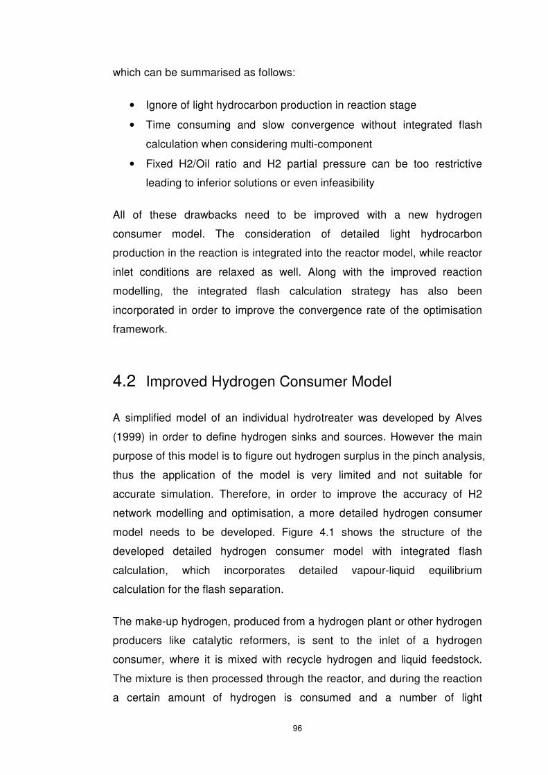
96
which can be summarised as follows:
• Ignore of light hydrocarbon production in reaction stage
• Time consuming and slow convergence without integrated flash
calculation when considering multi-component
• Fixed H2/Oil ratio and H2 partial pressure can be too restrictive
leading to inferior solutions or even infeasibility
All of these drawbacks need to be improved with a new hydrogen
consumer model. The consideration of detailed light hydrocarbon
production in the reaction is integrated into the reactor model, while reactor
inlet conditions are relaxed as well. Along with the improved reaction
modelling, the integrated flash calculation strategy has also been
incorporated in order to improve the convergence rate of the optimisation
framework.
4.2 Improved Hydrogen Consumer Model
A simplified model of an individual hydrotreater was developed by Alves
(1999) in order to define hydrogen sinks and sources. However the main
purpose of this model is to figure out hydrogen surplus in the pinch analysis,
thus the application of the model is very limited and not suitable for
accurate simulation. Therefore, in order to improve the accuracy of H2
network modelling and optimisation, a more detailed hydrogen consumer
model needs to be developed. Figure 4.1 shows the structure of the
developed detailed hydrogen consumer model with integrated flash
calculation, which incorporates detailed vapour-liquid equilibrium
calculation for the flash separation.
The make-up hydrogen, produced from a hydrogen plant or other hydrogen
producers like catalytic reformers, is sent to the inlet of a hydrogen
consumer, where it is mixed with recycle hydrogen and liquid feedstock.
The mixture is then processed through the reactor, and during the reaction
a certain amount of hydrogen is consumed and a number of light
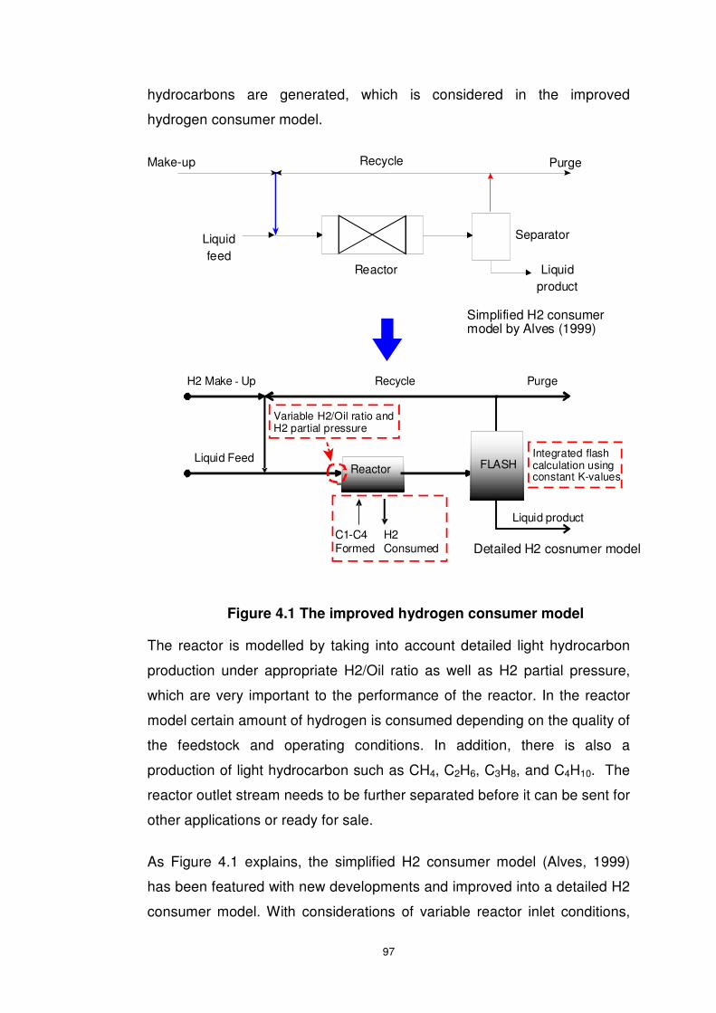
97
hydrocarbons are generated, which is considered in the improved
hydrogen consumer model.
Reactor
FLASH
H2 Make - Up
Liquid Feed
Liquid product
Purge
Recycle
C1-C4 Formed
H2 Consumed
Variable H2/Oil ratio andH2 partial pressure
Integrated flashcalculation usingconstant K-values
Purge
Liquid
feedLiquid
product
Make-up Recycle
Reactor
Separator
Simplified H2 consumermodel by Alves (1999)
Detailed H2 cosnumer model
Figure 4.1 The improved hydrogen consumer model
The reactor is modelled by taking into account detailed light hydrocarbon
production under appropriate H2/Oil ratio as well as H2 partial pressure,
which are very important to the performance of the reactor. In the reactor
model certain amount of hydrogen is consumed depending on the quality of
the feedstock and operating conditions. In addition, there is also a
production of light hydrocarbon such as CH4, C2H6, C3H8, and C4H10. The
reactor outlet stream needs to be further separated before it can be sent for
other applications or ready for sale.
As Figure 4.1 explains, the simplified H2 consumer model (Alves, 1999)
has been featured with new developments and improved into a detailed H2
consumer model. With considerations of variable reactor inlet conditions,

98
light hydrocarbons production during reaction and detailed flash calculation,
the newly developed multi-component hydrogen consumer model is able to
be used for hydroprocessing unit modelling and simulation or integrated
into a hydrogen network for optimisation.
Reactor FLASH
H2 Make - Up
Liquid Feed
Liquid product
Recycle
C1-C4
Formed
H2
Consumed
Feed Mixing Reaction Flash Calculation
Purge
Flash
Figure 4.2 Model construction of a H2 consuemr
The structure of the improved hydrogen consumer model can be found in
Figure 4.2 which can be divided into three different sections for detailed
modelling:
• Feed mixing
• Reaction (hydrotreating or hydrocracking)
• Flash separation
Each section is modelled under multi-component considerations. The
formulation is mainly based on mass balance. Practical constants have
been included. The detailed formulation equations are shown in following
sections.
4.2.1 Feed Mixing
The feed mixing model is used to calculate the mass balance at the inlet of

99
a hydrotreater. Basically there are three streams involved, including:
• Make-up hydrogen
• Liquid feedstock
• Recycle hydrogen
Liquid Feedstock
Mix Point
Fmix, Ymix
Make-up hydrogen Recycle hydrogen
To Reactor
Figure 4.3 Sink mass balances
The balance among these streams can be demonstrated in Figure 4.3. The
mathematical formulation can be expressed as follows:
jFFF jrejmujmix ∀+= ,,, (4.1)
jiYFYFYF jirejrejimujmujimixjmix ∀∀⋅+⋅=⋅ ,,,,,,,,, (4.2)
jFFFF jfeedjrejmujri ∀++= ,,,, (4.3)
jiYFYFYFYF jifeedjfeedjirejrejimujmujirijri ∀∀⋅+⋅+⋅=⋅ ,,,,,,,,,,,, (4.4)
Where Ffeed,j, Fmu,j, Fre,j and Fmix,j represent the flowrates of liquid feedstock,
make-up stream, recycle stream and the mix stream (mixture of make-up
and recycle streams) of consumer j respectively, while Yfeed,i,j, Ymu,i,j, Yre,i,j
and Ymix,i,j stand for the purity of component i in feedstock, make-up stream,
recycle stream and mix stream of consumer j. Subscripts i is used to
indicate each component such as H2 or impurities in a stream. The
subscripts j indicates different hydrogen consumers. In this way hydrogen
and all impurity components are considered to accomplish the multi-
component hydrogen consumer modelling for each H2 consumer in a H2

100
network. With Equations 4.1 to 4.4, the mass balance including hydrogen
balance and impurity balance for the three streams around the hydrogen
consumer inlet are maintained.
As Figure 4.3 shows, the mixing point is defined as the mixture of make-up
hydrogen and recycled hydrogen at the inlet of the reactor. The mixing
point represents the amount of hydrogen and its purity going into the
reactor along with the liquid feed. When considering a H2 network, a
hydrogen consumer can also receive hydrogen from other hydrogen
consumer’s purge gas, which may be rich in hydrogen. Details of hydrogen
network modelling can be found in Chapter 5.
4.2.2 Hydroprocessing Reaction
The reactor model is essential to the overall hydrotreater model. The liquid
feedstock is mixed with hydrogen and then sent through the
hydroprocessing reactor. The hydrogen-consuming reaction removes
sulphur, nitrogen and metals content and meanwhile saturates olefins and
some aromatics.
Reactor inletReactor
Flash inlet
C1-C4formed
HydrogenCosumptionR
Figure 4.4 Reactor model
One of the key improvements within this new model is the inclusion of light
hydrocarbon production, which is defined as R. For a specific case R is
involved in the calculation as a constant matrix depending on different
hydroprocessing units in the network. R can be used to express hydrogen
consumption and light hydrocarbon production simultaneously. The light
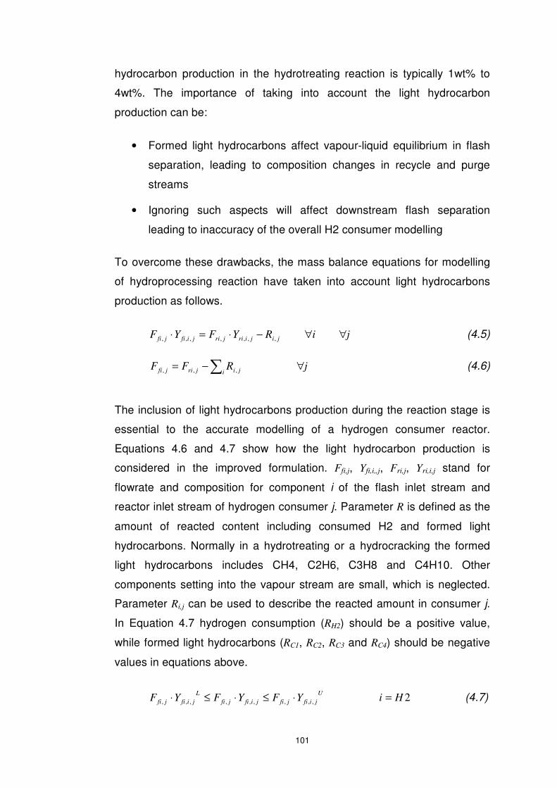
101
hydrocarbon production in the hydrotreating reaction is typically 1wt% to
4wt%. The importance of taking into account the light hydrocarbon
production can be:
• Formed light hydrocarbons affect vapour-liquid equilibrium in flash
separation, leading to composition changes in recycle and purge
streams
• Ignoring such aspects will affect downstream flash separation
leading to inaccuracy of the overall H2 consumer modelling
To overcome these drawbacks, the mass balance equations for modelling
of hydroprocessing reaction have taken into account light hydrocarbons
production as follows.
jiRYFYF jijirijrijifijfi ∀∀−⋅=⋅ ,,,,,,, (4.5)
jRFFi jijrijfi ∀−= ∑ ,,, (4.6)
The inclusion of light hydrocarbons production during the reaction stage is
essential to the accurate modelling of a hydrogen consumer reactor.
Equations 4.6 and 4.7 show how the light hydrocarbon production is
considered in the improved formulation. Ffi,j, Yfi,i,,j, Fri,j, Yri,i,j stand for
flowrate and composition for component i of the flash inlet stream and
reactor inlet stream of hydrogen consumer j. Parameter R is defined as the
amount of reacted content including consumed H2 and formed light
hydrocarbons. Normally in a hydrotreating or a hydrocracking the formed
light hydrocarbons includes CH4, C2H6, C3H8 and C4H10. Other
components setting into the vapour stream are small, which is neglected.
Parameter Ri,j can be used to describe the reacted amount in consumer j.
In Equation 4.7 hydrogen consumption (RH2) should be a positive value,
while formed light hydrocarbons (RC1, RC2, RC3 and RC4) should be negative
values in equations above.
2,,,,,,,,, HiYFYFYFU
jifijfijifijfi
L
jifijfi =⋅≤⋅≤⋅ (4.7)

102
2,,,,,, HiYYYU
jifijifi
L
jifi =≤≤ (4.8)
For a hydrogen consumer reactor, practical constraints for reactor inlet
conditions need to be considered. Rather than maintaining reactor inlet
conditions, by unfixing the H2/Oil ratio and H2 partial pressure at reactor
inlets (Zhang et al., 2008), they can be relaxed and also constrained in an
acceptable range in order to expand optimisation searching space and help
convergence. H2/Oil can be controlled by setting upper and lower bound
parameters for the amount of pure hydrogen going into reactor, whilst the
H2 partial pressure can be controlled by setting upper bound and lower
bound parameters for the hydrogen purity at the reactor inlet. With
Equations 4.8 and 4.9, the variable H2/Oil ratio and H2 partial pressure
strategy is implemented into the hydrogen consumer model.
4.2.3 Flash Separation
The reactor outlet needs to be separated into liquid and vapour. The liquid
phase will be further processed or blended into products before selling,
whilst the vapour will be either recycled for reuse or purged to a site fuel
system.
FlashFlash inlet
Recycle
Liquid product
Purge
Figure 4.5 Flash separation model
In the newly developed flash model as shown in Figure 4.5, the flash inlet

103
stream is sent from the reactor outlet and is separated into vapour and
liquid. To reflect the flash separation, a general method for flash calculation
is to make use of vapour-liquid equilibrium constants, commonly known as
the K-values, to describe the situation of flash separation. Basically the
separation can be expressed in terms of K-values in a general equation:
jiKYY jijiiqljivap ∀∀⋅= ,,,,, (4.9)
Where Yvap,i,j and Yliq,i,j stand for the composition of component i in vapour
or liquid from the flash unit of consumer j. The vapour-liquid equilibrium
constant, Ki,j, is used to represent the K-value for component i used for
flash calculation in consumer j. Combining the flash separation equation
with other mass balance equations, the whole hydrogen consumer flash
model can be expressed as:
jFFFF jpujliqjrejfi ∀++= ,,,, (4.10)
jiYFYFYFYF jipujpujiliqjliqjirejrejifijfi ∀∀⋅+⋅+⋅=⋅ ,,,,,,,,,,,, (4.11)
jFFF jliqjvapjfi ∀+= ,,, (4.12)
jFFF jpujrejvap ∀+= ,,, (4.13)
jiYY jirejivap ∀∀= ,,,, (4.14)
jYi jivap ∀=∑ 1,, (4.15)
jYi jiliq ∀=∑ 1,, (4.16)
jFF jjCHjre ∀= ,,2, (4.17)
Ffi,j, Fre,j, Fpu,j, Fvap,j and Fliq,j denote the flowrate of flash inlet stream,
recycle, purge, flash outlet vapour and flash outlet liquid of consumer j,
while Yfi,i,j, Yre,i,j, Ypu,i,j,, Yvap,i,j and Yliq,i,jj represent the relative composition of
component i in each stream mentioned above. Equations 4.11 to 4.13
express the mass balance for the flash separation. The recycle hydrogen
has the same purity as the flash vapour as shown in Equation 4.14. To
make sure the feasibility of the flash calculation, the summation of

104
compositions for all components in vapour or liquid stream is forced to be
equal to 1 to maintain the components balance. Variable FH2C,j,j is defined
as the hydrogen flowrate from hydrogen consumer j to j which is actually
the internal recycle hydrogen of consumer j. For modelling of a hydrogen
network, the hydrogen transportation between hydrogen consumers will be
shown in terms of this variable with different subscripts.
As for the previous optimisation method (Zhang et al., 2008), the K-values
need to be calculated at every iteration for an accurate separation result. It
brought excessive amount of calculation into the optimisation steps and
considerably time-consuming. Meanwhile, convergence problems could
occur during the large number of iterations, which is another drawback.
To overcome the drawbacks, the constant K-values strategy is introduced.
By using constant K-values for all iterations rather than calculating it every
time, it not only speeds up the optimisation procedure but also prevents it
from major convergence issues. The constant K-values strategy will be
discussed in more details with a complete verification procedure followed in
the next section.
Another issue with the flash modelling is the selection of the property
package. For a hydrocarbon-rich process there are mainly three popular
property packages to choose from:
• Peng-Robinson
• Soave-Redlich-Kwong (SRK)
• Grayson Streed
Grayson Streed is featured with special treatment on hydrogen content.
Therefore it is widely acknowledged as the most suitable property package
for simulating a stream with heavy hydrocarbons and high hydrogen
content, such as hydrotreating or hydrocracking process.
4.2.4 Detailed H2 Consumer Modelling Summary

105
Reactor
H P FLASH
Fmu, Ymu
H2 Make-Up
Ffeed, Yfeed
Reactor Inlet
Fri, Yri
Liquid Feed
Mix Point Fmix, Ymix
Flash Inlet
Ffi, Yfi
Recycle
Fre, Yre
C1-C4
Formed H2 Consumed
'Mix point fixed to maintainthe reactor inlet operatingconditons
'Hydrogen sink mass andmaterial balance calculated
'Reactor model forhydrotreater andhydrocracker separately
'Light hydrocarbonproduction included
'Integrated flashcalculation
'Constant K-valuesstrategy
liquid product
Purge
Figure 4.6 The improved hydrocracker model
As shown in Figure 4.6, the detailed hydrogen consumer model is
completed by connecting up the three main sections: feed mixing, reaction
and flash separation, which have been discussed in details with all relevant
formulation equations. As one of the major improvements, the reaction
modelling takes into account the light hydrocarbon production. In addition,
the flash separation is incorporated with constant K-values for flash
calculation. The details of integrated flash calculation with constant K-
values are discussed in the next section.
4.3 Integrated Flash Calculation with Constant K-
values
4.3.1 Introduction of Integrated Flash Calculation
One of the major improvements over the previous hydrogen network
optimisation methodology (Zhang et al., 2008) is the integrated flash
calculation with constant K-values strategy. In the existing optimisation
methodology (Zhang et al., 2008), the hydrogen network optimisation is
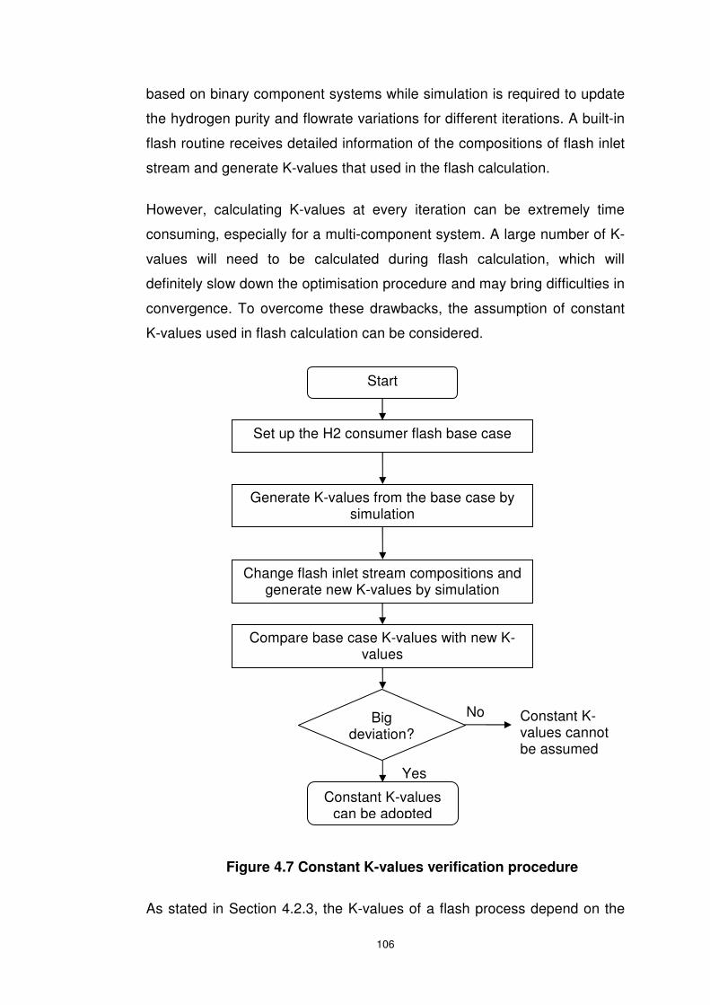
106
based on binary component systems while simulation is required to update
the hydrogen purity and flowrate variations for different iterations. A built-in
flash routine receives detailed information of the compositions of flash inlet
stream and generate K-values that used in the flash calculation.
However, calculating K-values at every iteration can be extremely time
consuming, especially for a multi-component system. A large number of K-
values will need to be calculated during flash calculation, which will
definitely slow down the optimisation procedure and may bring difficulties in
convergence. To overcome these drawbacks, the assumption of constant
K-values used in flash calculation can be considered.
Figure 4.7 Constant K-values verification procedure
As stated in Section 4.2.3, the K-values of a flash process depend on the
Start
Set up the H2 consumer flash base case
Change flash inlet stream compositions and generate new K-values by simulation
Compare base case K-values with new K-values
Constant K-values can be adopted
Big deviation?
No
Yes
Generate K-values from the base case by simulation
Constant K-values cannot be assumed

107
operating conditions including temperature and pressure. In addition, K-
values are also affected by compositions of the flash inlet stream to a very
small extent. Normally in refineries, the operating conditions of a flash unit
in a hydrogen consumer stay stable with very negligible change.
Considering the stable operating conditions, K-values are only related to
the flash inlet stream compositions. Since the influence of different
compositions on variation of K-values is very limited, there is a possibility
that K-values can be treated as constants.
The Constant K-values strategy allows us to integrate the flash calculation
into optimisation step without calculating K-values by simulation at every
iteration. However, it is needed to prove that whether the impact of flash
inlet stream composition on K-values is negligible or not.
As Figure 4.7 shows, the verification procedure of constant k-values starts
with the base case for a flash unit in a hydrogen consumer. The base case
model involves a stream going into the flash unit where it gets separated
into vapour and liquid. After building up the base case, simulation runs to
generate the K-values for the base case under specified operating
conditions. Then the flash inlet stream compositions are changed and the
flash unit will be simulated for each of them to generate new K-values for
each set of compositions. Note that in this procedure the operating
conditions including temperature and pressure are remained exactly the
same as those of the base case. The new K-values are compared with the
base case K-values, and the deviations between them will be checked to
see whether the constant K-value strategy is appropriate or not.
4.3.2 Results of Constant K-values Verification
In this work, ASPEN HYSYS (version 2006.5) software suite is used for the
verification. It is widely used and accepted as a simulation tool in chemical
engineering for modelling and simulation of refining or petrochemical
processes.

108
A general standard flash separation unit can be found in the HYSYS library.
The feed stream can be defined using one of the HYSYS built-in property
packages, Grayson-Streed, as it is designed to model streams with high
hydrogen content.
As for the base case, the flowrate and compositions of the feed stream is
set to be a sample of a naphtha hydrotreater reactor outlet stream. The
operating temperature and pressure for the flash unit has been set to
common flash conditions.
Table 4.1 Typical operating temperature and pressure for a
hydrotreater
Flash operating conditions settings
Temperature (oC) 50
Pressure (bara) 18
The specified operating conditions are shown in Table 4.1. As the
simulation is completed, the flowrate and compositions of each flash outlet
stream will be available and the k-values for the flash calculation can be
generated.
FLASH
Liquid
Vapour
Feed
Figure 4.8 Constant K-values verification
The flash unit base case is modelled in HYSYS as Figure 4.8 shows. A
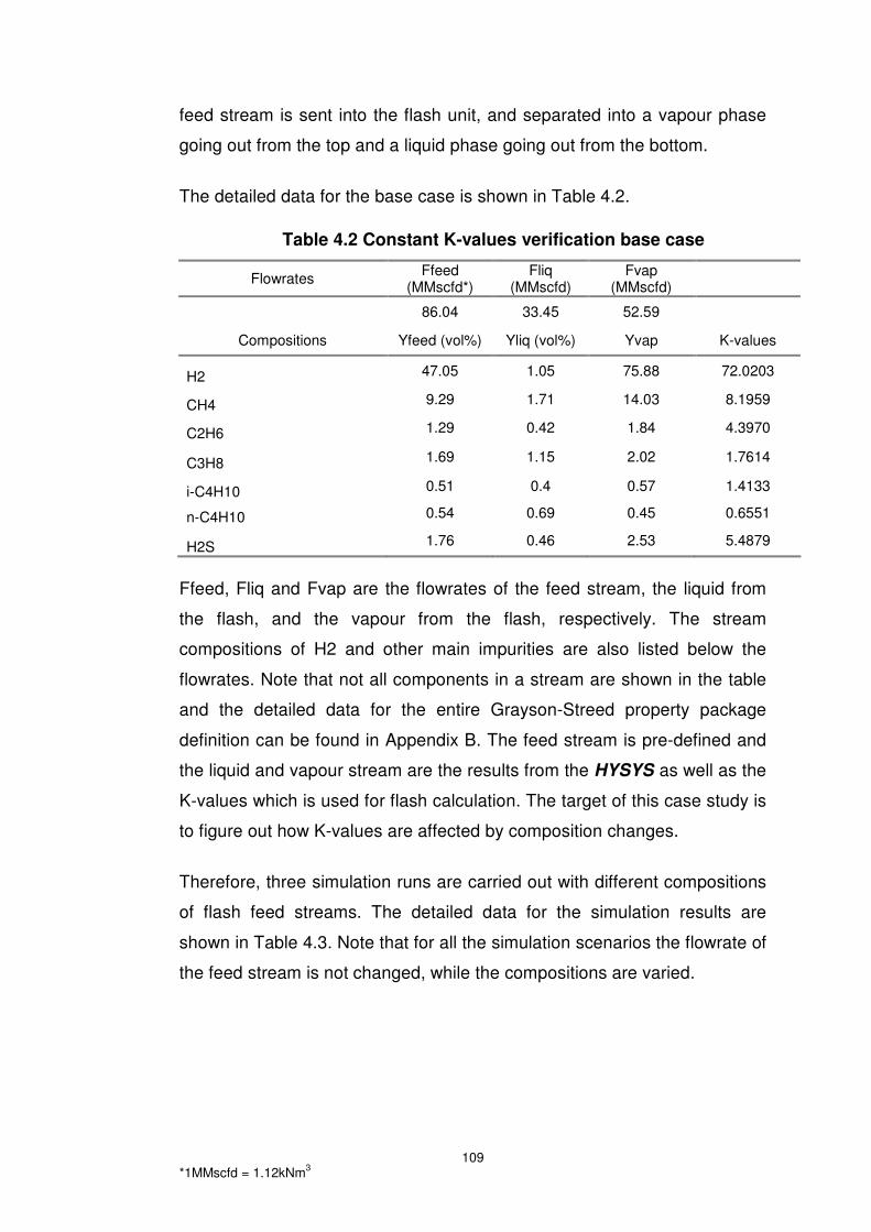
*1MMscfd = 1.12kNm
3
109
feed stream is sent into the flash unit, and separated into a vapour phase
going out from the top and a liquid phase going out from the bottom.
The detailed data for the base case is shown in Table 4.2.
Table 4.2 Constant K-values verification base case
Flowrates Ffeed
(MMscfd*) Fliq
(MMscfd) Fvap
(MMscfd)
86.04 33.45 52.59
Compositions Yfeed (vol%) Yliq (vol%) Yvap K-values
H2 47.05 1.05 75.88 72.0203
CH4 9.29 1.71 14.03 8.1959
C2H6 1.29 0.42 1.84 4.3970
C3H8 1.69 1.15 2.02 1.7614
i-C4H10 0.51 0.4 0.57 1.4133
n-C4H10 0.54 0.69 0.45 0.6551
H2S 1.76 0.46 2.53 5.4879
Ffeed, Fliq and Fvap are the flowrates of the feed stream, the liquid from
the flash, and the vapour from the flash, respectively. The stream
compositions of H2 and other main impurities are also listed below the
flowrates. Note that not all components in a stream are shown in the table
and the detailed data for the entire Grayson-Streed property package
definition can be found in Appendix B. The feed stream is pre-defined and
the liquid and vapour stream are the results from the HYSYS as well as the
K-values which is used for flash calculation. The target of this case study is
to figure out how K-values are affected by composition changes.
Therefore, three simulation runs are carried out with different compositions
of flash feed streams. The detailed data for the simulation results are
shown in Table 4.3. Note that for all the simulation scenarios the flowrate of
the feed stream is not changed, while the compositions are varied.
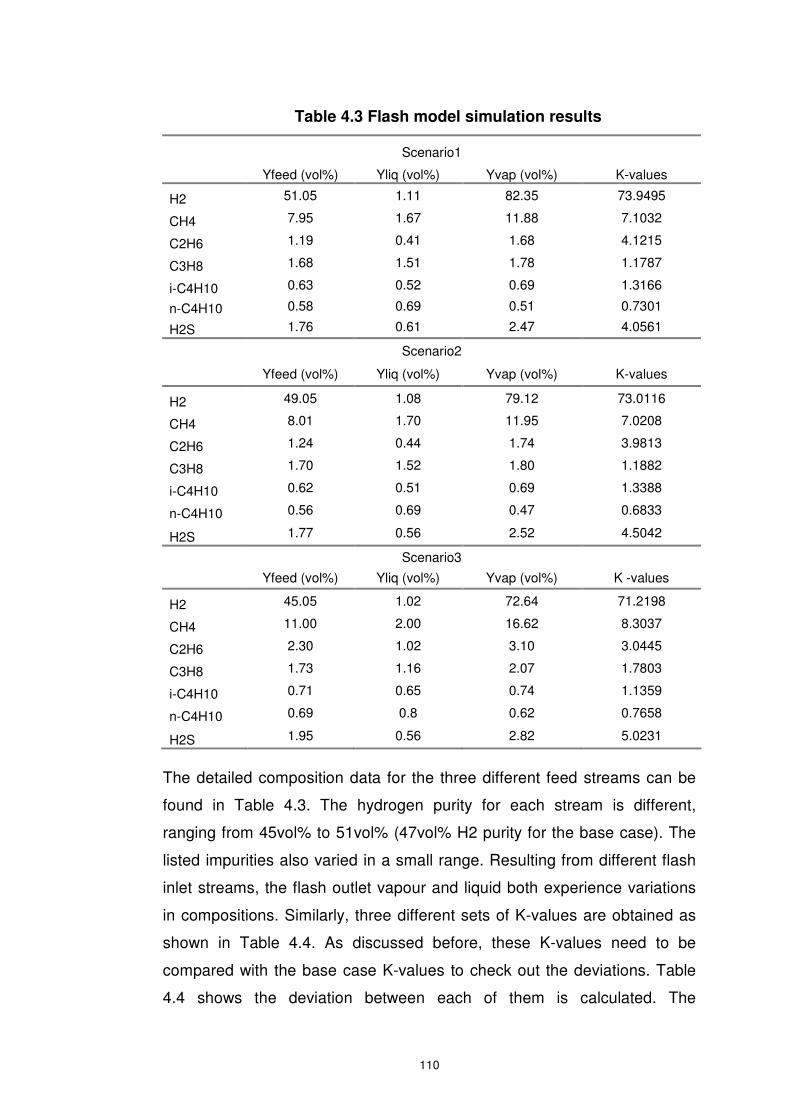
110
Table 4.3 Flash model simulation results
Scenario1
Yfeed (vol%) Yliq (vol%) Yvap (vol%) K-values
H2 51.05 1.11 82.35 73.9495
CH4 7.95 1.67 11.88 7.1032
C2H6 1.19 0.41 1.68 4.1215
C3H8 1.68 1.51 1.78 1.1787
i-C4H10 0.63 0.52 0.69 1.3166
n-C4H10 0.58 0.69 0.51 0.7301
H2S 1.76 0.61 2.47 4.0561
Scenario2
Yfeed (vol%) Yliq (vol%) Yvap (vol%) K-values
H2 49.05 1.08 79.12 73.0116
CH4 8.01 1.70 11.95 7.0208
C2H6 1.24 0.44 1.74 3.9813
C3H8 1.70 1.52 1.80 1.1882
i-C4H10 0.62 0.51 0.69 1.3388
n-C4H10 0.56 0.69 0.47 0.6833
H2S 1.77 0.56 2.52 4.5042
Scenario3
Yfeed (vol%) Yliq (vol%) Yvap (vol%) K -values
H2 45.05 1.02 72.64 71.2198
CH4 11.00 2.00 16.62 8.3037
C2H6 2.30 1.02 3.10 3.0445
C3H8 1.73 1.16 2.07 1.7803
i-C4H10 0.71 0.65 0.74 1.1359
n-C4H10 0.69 0.8 0.62 0.7658
H2S 1.95 0.56 2.82 5.0231
The detailed composition data for the three different feed streams can be
found in Table 4.3. The hydrogen purity for each stream is different,
ranging from 45vol% to 51vol% (47vol% H2 purity for the base case). The
listed impurities also varied in a small range. Resulting from different flash
inlet streams, the flash outlet vapour and liquid both experience variations
in compositions. Similarly, three different sets of K-values are obtained as
shown in Table 4.4. As discussed before, these K-values need to be
compared with the base case K-values to check out the deviations. Table
4.4 shows the deviation between each of them is calculated. The

111
deviations between new generated K-values and the base case K-values
are very limited. In Scenario 1, the biggest deviation is +1.9292 for H2
component, while all other deviations are within +/-1.1. Similarly for
Scenario 2, all deviations are within +/-1.2. For Scenario 3, the biggest
deviation for K-values comparison happens to C2H6 component, which is
however, only -1.35. Again, all other K-values deviations appear no more
than +/-1.
To summarise comparison, it shows some but very limited deviations for
the K-values of all components, which indicates that using constant K-
values is a reasonable assumption to deal with different flash inlet stream
with varying compositions in optimisation. However, after obtaining the
optimisation result, re-simulation is necessary to correct certain deviations
caused by the assumption of constant K-values.
Table 4.4 Flash model base case and simulations comparison
Base case K-values K-values of scenario 1 Deviation
H2 72.0203 73.9495 1.9292
CH4 8.1959 7.1032 -1.0927
C2H6 4.3970 4.1215 -0.2755
C3H8 1.7614 1.1787 -0.5828
i-C4H10 1.4133 1.3166 -0.0966
n-C4H10 0.6551 0.7301 0.0751
H2S 4.8685 4.0561 -0.8125
Base case K K of scenario 2 Deviation
H2 72.0203 73.0116 0.9913
CH4 8.1959 7.0208 -1.1751
C2H6 4.3970 3.9813 -0.4157
C3H8 1.7614 1.1882 -0.5733
i-C4H10 1.4133 1.3388 -0.0745
n-C4H10 0.6551 0.6833 0.0282
H2S 4.8685 4.5042 -0.3643
Base case K K of scenario 3 Deviation
H2 72.0203 71.2198 -0.8005
CH4 8.1959 8.3037 0.1078
C2H6 4.3970 3.0445 -1.3525
C3H8 1.7614 1.7803 0.0188
i-C4H10 1.4133 1.1359 -0.2774
n-C4H10 0.6551 0.7658 0.1107
H2S 4.8685 5.0231 0.1546

112
Therefore, for a hydrogen network optimisation problem, the integrated
flash calculation with constant K-values can be incorporated in the
optimisation procedure with 2 steps:
1. K-values are initially obtained from rigorous flash calculation in
simulation
2. Then K-values will be checked by using simulation when
optimisation results are obtained.
The main advantages of integrated flash calculation using constant K-
values in optimisation include:
• More accurate optimisation methodology
• More reliable and efficient flash calculation
• Huge time and computing resource saving compared with the
existing approach by (Zhang et al., 2008)
Although the integrated flash calculation with the constant K-values
strategy has been verified, it has to be careful when incorporating it into the
optimisation of a hydrogen network, due to the complexity and uncertainty
of a complicated hydrogen network. As a result, for each optimisation
procedure, the K-values for flash calculation in each hydrogen consumer
model will be initialised and assumed as constant from the base case
simulation. When the optimisation result is obtained, the K-values
generated from the optimisation solutions will need to be verified in order to
ensure the feasibility of the optimisation results. Detailed discussion and
application of the optimisation framework with constant K-values can be
found with a case study in Chapter 5.
4.4 Summary
A detailed general hydrogen consumer model has been proposed under
multi-component consideration. The main features and advantages for the
detailed hydrogen consumer model are as follows:

113
• Inclusion of light hydrocarbon production
• Variable H2/Oil ratio and H2 partial pressure
• Integrated flash calculation
These improvements are developed based on the existing hydrogen
consumer model (Zhang et al., 2008). Firstly, light hydrocarbon production
during hydroprocessing reaction is now considered and represented by
mass balance calculations in reactor modelling. Furthermore, the reaction
inlet conditions are allowed to vary slightly instead of strictly fixed, in order
to open up the degrees of freedom for the hydrogen network optimisation.
Also, the flash calculation is incorporated to take into account vapour-liquid
equilibrium under multi-components.
It is the most detailed hydrogen consumer model for H2 network
management so far, and will be used in the detailed hydrogen network
modelling and optimisation, which will be discussed in Chapter 5.
Another major improvement over the previous work by (Zhang et al., 2008)
is the introduction of integrated flash calculation using constant K-values, in
the optimisation model.
By using the constant K-values, the flash calculation for each hydrogen
consumer can be integrated into optimisation without the need of iterative
simulation. The constant K-values assumption has been verified for its
feasibility. The integrated flash calculation can simplify the whole
optimisation procedure with significantly reduced computation time and
much more improved calculation efficiency.

114
Chapter 5 Multi-component Optimisation
for H2 networks
5.1 Overall Hydrogen Network Modelling and
Optimisation
In Chapter 4, the detailed hydrogen consumer model with multiple
components has been developed. However, to complete an overall
hydrogen network, we still need to involve models of hydrogen producers
and site fuel systems. Considering hydrogen consumers as a core of a
hydrogen network, they need to receive hydrogen from hydrogen
producers and may purge hydrogen to a site fuel system. Therefore, to
complete a hydrogen network model, the balance among hydrogen
consumers, producers and fuel system needs to be modelled.
5.1.1 Hydrogen Producer Model
In this work, a shortcut model for a general hydrogen producer is
developed, which simply provides make-up hydrogen to hydrogen
consumers with a flowrate and composition.
H2 Producer
Make-up H2
Figure 5.1 Short-cut hydrogen producer model
In refineries, the make-up hydrogen mainly comes from hydrogen
producers including hydrogen plants and/or other purified by-product
hydrogen, for example catalytic reformers or ethylene plants. The H2 purity
of different hydrogen producers may vary. Therefore, with different flowrate
and H2 purity specifications, the general hydrogen producer model can be

115
adjusted to a various hydrogen producer models. The relationship between
hydrogen producers and consumers can be represented by mass balance.
jFFF jmixj jjCHk jkPH ∀=+ ∑∑ ,1 ,1,2,,2 (5.1)
jYFYFYF jimixjmixj jiCHjjCHk kiPHjkPH ∀⋅=⋅+⋅ ∑∑ ,,,1 1,,2,1,2,,2,,2 )()( (5.2)
FH2P,k,j denotes the flowrates of hydrogen production from producer k to
hydrogen consumer j. Subscript j1 is introduced as an alias of subscript j to
represent different consumers. Using subscripts j1 and j, FH2C,j1,j represents
the hydrogen transportation from consumer j1 to consumer j. When j1
equals j, it represents the internal recycle of consumer j (or j1). When j1 is
not equal to j, it represents the hydrogen flowrate from the purge gas of
consumer j1 to consumer j. YH2P,i,k and YH2C,i,j1 represent composition of
component i of hydrogen producer k and composition of component i of
hydrogen stream between consumers, respectively.
According to Equation 5.1 the summation of hydrogen production from
various hydrogen producers to consumer j plus recycle and hydrogen from
other consumers equals to the flowrate at the mixing point of consumer j,
which is a hydrogen sink. Combined with Equation 5.2 which represents
component balance between sinks and sources, the complete mass
balance between hydrogen producers and consumers is modelled.
5.1.2 Site Fuel Balance
In a hydrogen network, a site fuel system is used to collect the purge gas
from various hydrogen consumers. Normally the purge gas comes from the
flash vapour in a hydrogen consumer. Figure 5.2 shows an example of a
site fuel system. Four hydrotreaters purge gas from their high pressure
flash to the site fuel. The site fuel system is important to a hydrogen
network, as it maintains the overall hydrogen network mass balance.
The purge gas flowrate and purities can be obtained from the flash model
proposed in Chapter 4. Note that the compositions of a purge stream are

116
exactly the same as the recycle, as they are both generated from the high
pressure flash.
Site Fuel
Hydrotreater1 Purge
Hydrotreater2 Purge
Hydrotreater3 Purge
Hydrotreater4 Purge
FPUh2c,YPUh2ci
FPUh2c,YPUh2ci
FPUh2c,YPUh2ci
FPUh2c,YPUh2ci
Figure 5.2 An example of site fuel model for a hydrogen network
The hydrogen producer model is connected to the inlets of hydrogen
consumers, and the site fuel model needs to be connected to the outlets of
hydrogen consumers. The relationship between hydrogen consumers and
a site fuel system is represented as follows:
jjjFFFj jjCHjSFjpu ∀≠+= ∑ 11 1,,2,, (5.3)
jjjYFYFYFj jiCHjjCHjiSFjSFjipujpu ∀≠⋅+⋅=⋅ ∑ 1)(1 ,,21,,2,,,,,, (5.4)
jiYYY jiCHjiSFjipu ∀∀== ,,2,,,, (5.5)
Fpu,j and FSF,j represent the flowrate of the total purge gas of consumer j and
the amount sent to the site fuel system. When 1jj ≠ , FH2C,j,j1 excludes the
internal recycle of consumer j, and represents the hydrogen flowrate from
the purge gas of consumer j to consumer j1. Equation 5.3 explains the
possible destination of purge gas from a hydrogen consumer. Normally the
purge gas is generated from the flash separation and can be sent to a site
fuel system or feed other consumers if it contains rich enough hydrogen.
As shown in Equation 5.3, the total amount of purge gas from consumer j

117
equals to the site fuel contribution from consumer j plus the summation of
hydrogen sent to other consumers from consumer j.
Ypu,i,j, YSF,i,j, and YH2C,i,j represent compositions of purge, purge to site fuel
and recycle streams, which are actually the same because they are all from
the same source, the flash vapour phase.
Together with Equations 4.1-4.17 for detailed hydrogen consumer models,
a hydrogen network is modelled by incorporating Equations 5.1 to 5.5,
which represent mass balance among hydrogen producers, consumers
and a site fuel system.
5.1.3 Overall Multi-component H2 Network Modelling
The H2 network optimisation problem can be formulated by using a few
groups of definitions including variables, parameters, constraints, and
objectives.
� Variables:
Flowrates and purities of hydrogen streams around a hydrogen network
including hydrogen make-up, recycle, purge stream of each hydrogen
consumer and connections consumers and hydrogen plant. Some of
them are independent variables such as hydrogen production of
hydrogen producers, while others are dependent such as recycle
flowrate and purities, as these are calculated from flash calculations.
Details of variable declarations can be found in Appendix C.
� Parameters:
- Liquid feed stock properties
- reactor parameter R (hydrogen consumption and light
hydrocarbon production)
- K-values used for flash calculation
118
- Range of variable H2/Oil ratio and H2 partial pressure for
hydrogen consumer inlets
� Constraints:
All proposed equations in chapter 4 and chapter 5 are used as
constraints for the optimisation. Constraints for individual detailed
hydrogen consumer include Equations 4.1 to 4.17, 5.1 to 5.5 are used
as hydrogen network balance constraints.
� Objective function: minimise total required hydrogen production
[ ] 2)( ,,2,2 HiYFMINObj kiPHk kPH =⋅= ∑ (5.6)
Where Obj stands for the optimisation objective; FH2P,K represents the
flowrate of hydrogen production for each hydrogen producer and YH2P,i,k
denotes relative hydrogen production purity for each hydrogen producer.
As the objective function shows, the optimisation target is to minimise the
summation of all hydrogen production from all hydrogen utility producers
involved in hydrogen network.
For economic concerns, the objective function can be extended to minimise
the total operating cost for a hydrogen network by taking into account the
hydrogen production cost and fuel gas value.
[ ] 2)()( ,,2,2 HiUFUFMINObj jSFj jSFHk kPH =⋅−⋅= ∑∑ (5.7)
The total operating cost should involve both hydrogen production cost and
fuel gas value in the site fuel system. In Equation 5.7 the total operating
cost is represented by total hydrogen production cost minus total fuel gas
value, where UH2 and USF,j represent the unit price for hydrogen and fuel
gas respectively. It is suggested to calculate both unit prices based on
heating value contributions.
5.1.4 H2 Network Superstructure

119
The H2 network optimisation is based on a H2 network superstructure.
When considering optimisation for a hydrogen network, a couple of
questions must be considered beforehand.
For each hydrogen consumer:
� Make-up hydrogen: where and how much?
� Recycle hydrogen: how much?
Considering the make-up hydrogen at the inlet of each hydrogen consumer,
it is defined as a variable which can be obtained from various H2 producers
such as a hydrogen plant, CCR, an ethylene plant, etc. Meanwhile, the
purge gas from other consumers may contribute to the make-up hydrogen
as well. When dealing with a large and complicated hydrogen network with
many hydrogen consumers involved, the possibilities of sources for make-
up hydrogen can be plenty.
As for recycle hydrogen, each hydrogen consumer should decide the
flowrate of recycle hydrogen. As discussed before, the recycle is taken
from flash vapour and sent back to the consumer inlet, mixing with make-
up hydrogen. Therefore it is very sensitive to the overall H2 balance of the
consumer, and will affect the make-up hydrogen requirement due to the
reactor inlet conditions constraints.
To answer these questions systematically and quantitatively, we will need
to introduce a H2 network superstructure for optimisation. In a H2 network
superstructure, all hydrogen producers and consumers will be defined as
hydrogen sinks and sources. Hydrogen producers are defined as hydrogen
sources clearly. Hydrogen consumers are defined as sinks and sources at
the same time, as it can receive hydrogen from sources, meanwhile
provide hydrogen to other sinks (from its high pressure flash vapour). In
this way the H2 superstructure allows flexibility for the balance between
hydrogen sinks and sources, based on which the optimisation can exploit
the best solutions for a hydrogen network under constraints.

120
Figure 5.3 An example of hydrogen network superstructure
An example of hydrogen network superstructure is shown in Figure 5.3, the
network consists of five hydrogen sources, including a hydrogen plant and
sources A to D, and five hydrogen sinks including fuel and sinks A to D.
Typically, most of the hydrogen consumers would act as both sinks and
sources.
As Figure 5.3 shows, hydrogen can be transported from any source to any
sink. This is to give the maximum potential in the hydrogen network
superstructure to provide a large searching space for optimisation. On the
basis of this superstructure, an optimisation algorithm can search from
these possibilities and figure out the best solution. Therefore the hydrogen
superstructure is essential to the hydrogen network optimisation in this
work.
5.1.5 H2 Network Optimisation Framework
The optimisation framework for a multi-component H2 network is illustrated
in Figure 5.4. Starting with the hydrogen pinch analysis, the super-structure
based optimisation will be performed based on the proposed multi-
component hydrogen network model. The obtained optimisation result
needs to be verified by simulation for its feasibility.
H2 Plant
Source A
Source B
Source C
Source D
Sink A
Sink B
Sink C
Fuel
Sink D

121
Figure 5.4 The Multi-component hydrogen network optimisation
framework
The overall optimisation procedure can be summarised into 4 steps:
Step1: Hydrogen pinch analysis for base case
First, the base case is simulated and relevant data are extracted. Then the
hydrogen pinch analysis (Alves, 1999) is applied to check for system
potentials and scope for improvement, by comparing the current H2
consumption against the theoretical minimum H2 target. If there is a big
gap between current H2 utility flow and the target, the procedure continues.
Otherwise the optimisation stops or requires problem redefinition.
Step 2: Integrated hydrogen network optimisation
Start
Hydrogen pinch analysis for base case
Multi-component optimisation with integrated flash calculation
Simulation to verify K-values and network flows
Scope for Improvements
Optimal solution
∆ Obj ≤ έ No
Yes
Update H2 network model
Stop investigation or redefine problem
No
Check deviation between the two results

122
The overall H2 network model is optimised, in which the integrated flash
calculation is included in order to improve calculation efficiency and
accuracy, as discussed in Chapter 4.
Step 3: Network simulation
During the optimisation there is a key assumption that the K-values used
for flash calculation is considered as constants. However, changes in
network connections may result in slight variations in K-values, which may
affect the accuracy of the optimisation results. Therefore, network
simulation is carried out based on the updated network connections from
the optimisation result to retain feasibility.
Step 4: Optimality check
After retaining feasibility from the network simulation, all flowrates and
purities from simulation are compared the optimisation results. Only when
the tolerance between them is met, the optimisation results can be
approved. Otherwise the model is updated and optimised all over again.
5.1.6 Pseudo-components
For multi-component hydrogen network optimisation, all chemical
components in each stream around the hydrogen network need to be
specified with physical property information. Since the exact component
information would not be available due to petroleum mixture’s complexity,
the definition of components is in terms of both real and pseudo-
components.

123
Table 5.1 Properties of pseudo components
Pseudo-Components
TB (K)
API Gravity
Specific gravity
MW TC (K)
PC (bar)
PC1-NHT 344.30 68.4914 0.7075 89.92 523.70 33.69
PC2-NHT 368.50 67.9645 0.7094 102.9 545.57 28.97
PC3-NHT 390.00 65.6453 0.7177 114.8 566.46 26.11
PC4-NHT 412.80 62.1456 0.7307 127.9 589.51 23.86
PC5-NHT 434.00 58.5494 0.7445 140.7 611.25 22.20
PC1-CNHT 349.70 68.6665 0.7069 92.8 528.35 32.43
PC2-CNHT 376.40 67.4160 0.7114 107.3 552.97 27.76
PC3-CNHT 409.40 61.7406 0.7322 125.3 587.09 24.44
PC4-CNHT 436.60 58.0798 0.7464 142.3 613.95 22.02
PC5-CNHT 477.30 51.3646 0.7738 169.3 655.45 19.48
PC1-DHT 499.80 48.0363 0.7881 185.8 677.93 18.28
PC2-DHT 536.20 43.1501 0.8102 215 713.61 16.56
PC3-DHT 579.10 37.8757 0.8354 253.2 754.95 14.88
PC4-DHT 600.80 35.3928 0.8478 274.1 775.58 14.15
PC5-DHT 640.40 31.0198 0.8707 314.6 812.99 12.98
HC-GA1 287.10 76.9630 0.6788 67.36 463.63 46.57
HC-GA2 304.40 72.0910 0.6950 72.75 483.97 42.97
HC-GA3 320.20 67.8959 0.7096 78.11 502.34 40.12
HC-GA4 336.70 63.2102 0.7267 84.18 521.86 37.74
HC-GA5 353.90 68.6862 0.7068 95.05 532.06 31.54
HC-NAP1 349.00 68.6385 0.7070 92.42 527.75 32.59
HC-NAP2 374.10 67.5696 0.7108 106 550.83 28.10
HC-NAP3 399.30 64.3468 0.7225 120.1 575.74 25.10
HC-NAP4 421.10 60.7085 0.7362 132.8 598.06 23.19
HC-NAP5 446.30 56.3756 0.7532 148.4 623.96 21.37
HC-DIE1 438.00 57.8706 0.7472 143.2 615.35 21.91
HC-DIE2 484.90 50.2637 0.7785 174.8 663.01 19.05
HC-DIE3 529.90 43.9419 0.8065 209.7 707.51 16.84
HC-DIE4 575.20 38.3582 0.8330 249.6 751.18 15.02
HC-DIE5 618.40 33.4522 0.8578 291.8 792.19 13.60
The lighter components such as methane, propane, i-butane, n-butane can
be found from ASPEN HYSYS components library as real components.
The heavier part of the mixture can be calculated by using ASPEN HYSYS
internal components estimation function on the basis of true boiling point
and API gravity. Table 5.1 lists all of the pseudo-components included in
the multi-component model and their properties.
The liquid fractions can be classified into a number of groups based on true
boiling point (TBP). In addition, each group of components can be used to
represent a fuel product from a hydroprocessor such as gasoline or diesel.
All properties information for each pseudo-component can be found in
Table 5.1. These pseudo-components are used for modelling each stream

124
in a hydrogen network.
5.1.7 Selection of Optimisation Solvers
A variety of optimisation engines are available for multi-component
hydrogen network optimisation problems. Different specifications of
optimisation problems would require accordingly different optimisation
methodologies. Basically the optimisation algorithms to choose from can be
classified into two main groups:
• Deterministic method : Linear programming (LP), Non-Linear
programming (NLP) or Mixed Integer Non-Linear programming
(MINLP)
• Stochastic method: Simulated Annealing (SA), Genetic Algorithm
(GA), Tabu search, etc.
The deterministic methods are mainly gradient based approaches. They
are always fast in searching for solutions. However they do not perform
well when dealing with large scale mixed integer non-linear programming
problems and may be trapped in local optimum, if a problem is non-convex.
On the other hand, stochastic methods are random search methods with
relatively slow searching speed, but with great capability to solve mix
integer non-linear programming problems and converge to near-global
optimum solutions.
Both methodologies have got obvious advantages and disadvantages. In
this work the non-linear programming (NLP) approach is first chosen for the
multi-component H2 network optimisation method. In the following case
study GAMS (Version GAMS IDE 2.0.13.0.) is selected as the modelling
and optimisation tool with its built-in NLP solver.
5.2 Case Study

125
Based on the proposed multi-component H2 network modelling and
optimisation methodology, a case study is carried out using NLP algorithm.
5.2.1 Base Case
The base case carried out in this case study is originally from the hydrogen
consumer and hydrogen network model by (Singh, 2006). Figure 5.5 shows
the flowsheet of the hydrogen network base case. There are two hydrogen
producers undertaking hydrogen production and supply hydrogen to the
hydrogen network. As the main hydrogen source, the hydrogen plant
produces 109.6 MMscfd of hydrogen with high purity of 99 vol%. The
supporting hydrogen source is CCR which provides 14.63 MMscfd of
hydrogen with a relatively lower purity of 83 vol%.
H2 Plant
CCR
NHT
DHT
CNHT
HC
Fuel
109.6 MMscfd99.0 vol%
14.63 MMscfd83.0 vol%
6.675 MMscfd83.0 vol%
7.788 MMscfd83.0 vol%
25.090 MMscfd99.0 vol%
84.510 MMscfd99.0 vol%
32.22 MMscfd66.48 vol%
27.61 MMscfd76.57 vol%
67.75 MMscfd81.72 vol%
155.92 MMscfd71.38 vol%
5.34 MMscfd76.57 vol%.
3.323 MMscfd66.48 vol%
12.803 MMscfd71.38 vol%
7.885 MMscfd81.72vol%
Figure 5.5 Multi-component hydrogen network base case
As for hydrogen consumers, there are three different hydrotreaters and one
hydrocracker in the hydrogen network. Each of them is modelled with

126
certain amount of hydrogen consumption, and the hydrocracker is with the
largest hydrogen consumption. All hydrogen consumers are configured
with an internal recycle. All the purged gases from these hydrogen
consumers are collected in fuel gas system. In the current network there is
no hydrogen transportation between hydrogen consumers. Tables 5.2 and
5.3 shows network connections and the detailed data for each unit in the
hydrogen network.
Table 5.2 Details of network connections for each H2 consumer
NHT CNHT DHT HC FUEL
CCR 6.675 7.788 0.000 0.000 0.000
H2PLANT 0.000 0.000 25.090 84.510 0.000
NHT 76.57 0.000 0.000 0.000 5.34
CNHT 0.000 32.22 0.000 0.000 3.323
DHT 0.000 0.000 155.92 0.000 12.803
An overview of the hydrogen network distribution is summarised in Table
5.2. The flowrate of hydrogen from hydrogen producers to consumers are
shown. Also the flowrate of hydrogen between consumers are listed. The
hydrogen flowrate between the same consumers is used to indicate its
internal recycle hydrogen. Table 5.3 gives operating conditions for flash
units of each hydrogen consumer.
Table 5.3 Flash Operating conditions for each hydrogen
consumer
High pressure flash Temperature (oC) Pressure (bara)
NHT 50 18
CNHT 50 20
DHT 50 20
HC 50 160
For the four different H2 consumers, each of them is supposed to process
feedstock with different properties in order to produce relevant products.
For the hydrotreaters the feedstock is relatively light, while the
hydrocracker can take much heavier feedstock. Table 5.4 gives detailed
information of the feedstock for each hydrogen consumer including
flowrates and compositions for all components in the system. Note that the

127
liquid feedstock contains no hydrogen, and it will be mixed with make-up
and recycle hydrogen at the reactor inlet. For each individual hydrogen
consumer, the flowrate and complete compositions of hydrogen make-up,
recycle and purge are all provided.
Table 5.4 Detailed data of liquid feedstock for each H2 consumer
Feedstock NHT CNHT DHT HC
Flowrate(MMScfd) 32.79 12.95 36.15 37.62
Compositions (vol%)
H2 0.00 0.00 0.00 0.00
CH4 1.47 1.63 6.53 1.45
C2H6 0.62 1.30 2.74 1.35
C3H8 1.33 2.07 5.94 5.23
i-C4H10 0.43 0.67 1.93 8.31
n-C4H10 0.72 1.12 3.22 5.09
H2S 0.67 3.09 4.88 5.69
NH3 0.00 0.18 0.30 2.86
PC1-NHT 19.40 0.00 0.03 0.00
PC2-NHT 21.35 0.00 0.03 0.00
PC3-NHT 22.51 0.00 0.03 0.00
PC4-NHT 10.89 0.00 0.04 0.00
PC5-NHT 20.00 0.00 0.02 0.00
PC1-CNHT 0.14 11.61 0.00 0.00
PC2-CNHT 0.29 18.37 0.00 0.00
PC3-CNHT 0.18 22.63 0.00 0.00
PC4-CNHT 0.00 16.79 0.00 0.00
PC5-CNHT 0.00 20.54 0.00 0.00
PC1-DHT 0.00 0.00 7.52 0.00
PC2-DHT 0.00 0.00 15.20 0.00
PC3-DHT 0.00 0.00 19.47 0.00
PC4-DHT 0.00 0.00 23.95 0.00
PC5-DHT 0.00 0.00 8.17 0.00
HC-GA1 0.00 0.00 0.00 1.02
HC-GA2 0.00 0.00 0.00 2.03
HC-GA3 0.00 0.00 0.00 4.01
HC-GA4 0.00 0.00 0.00 2.54
HC-GA5 0.00 0.00 0.00 1.64
HC-NAP1 0.00 0.00 0.00 2.57
HC-NAP2 0.00 0.00 0.00 3.76
HC-NAP3 0.00 0.00 0.00 7.66
HC-NAP4 0.00 0.00 0.00 6.20
HC-NAP5 0.00 0.00 0.00 2.96
HC-DIE1 0.00 0.00 0.00 5.89
HC-DIE2 0.00 0.00 0.00 7.92
HC-DIE3 0.00 0.00 0.00 9.95
HC-DIE4 0.00 0.00 0.00 8.18
HC-DIE5 0.00 0.00 0.00 3.68
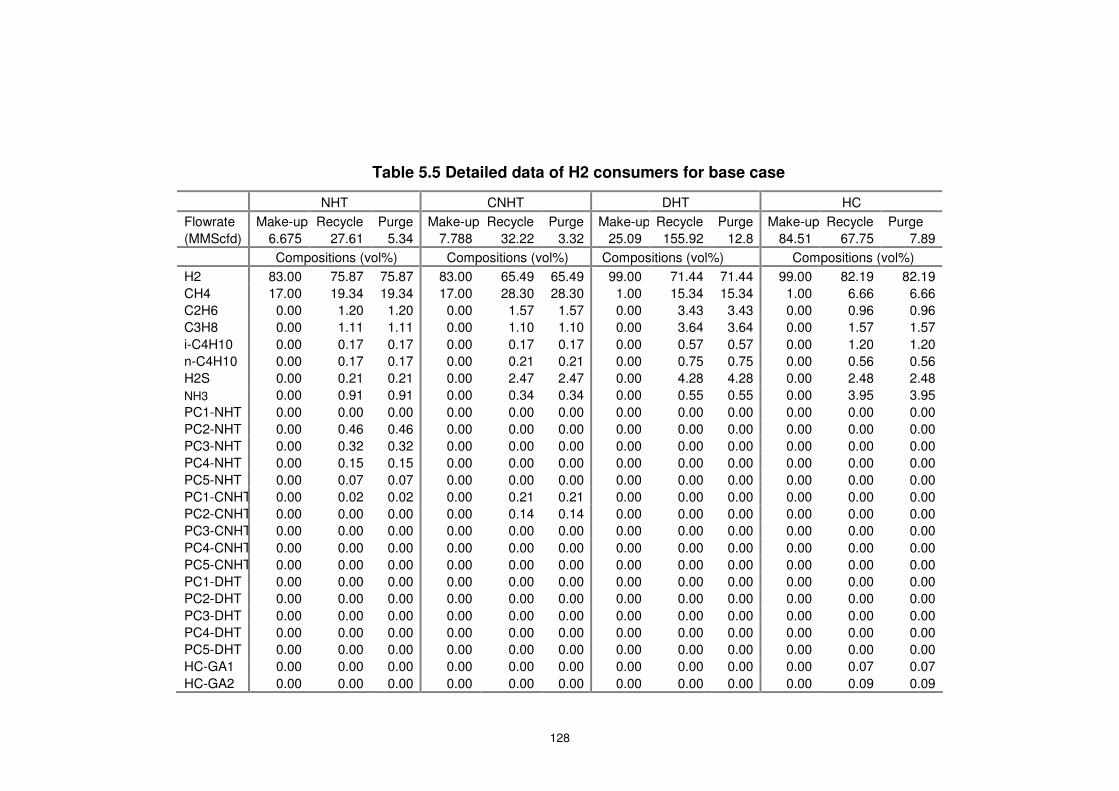
128
Table 5.5 Detailed data of H2 consumers for base case
NHT CNHT DHT HC
Flowrate Make-up Recycle Purge Make-up Recycle Purge Make-up Recycle Purge Make-up Recycle Purge
(MMScfd) 6.675 27.61 5.34 7.788 32.22 3.32 25.09 155.92 12.8 84.51 67.75 7.89
Compositions (vol%) Compositions (vol%) Compositions (vol%) Compositions (vol%)
H2 83.00 75.87 75.87 83.00 65.49 65.49 99.00 71.44 71.44 99.00 82.19 82.19
CH4 17.00 19.34 19.34 17.00 28.30 28.30 1.00 15.34 15.34 1.00 6.66 6.66
C2H6 0.00 1.20 1.20 0.00 1.57 1.57 0.00 3.43 3.43 0.00 0.96 0.96
C3H8 0.00 1.11 1.11 0.00 1.10 1.10 0.00 3.64 3.64 0.00 1.57 1.57
i-C4H10 0.00 0.17 0.17 0.00 0.17 0.17 0.00 0.57 0.57 0.00 1.20 1.20
n-C4H10 0.00 0.17 0.17 0.00 0.21 0.21 0.00 0.75 0.75 0.00 0.56 0.56
H2S 0.00 0.21 0.21 0.00 2.47 2.47 0.00 4.28 4.28 0.00 2.48 2.48
NH3 0.00 0.91 0.91 0.00 0.34 0.34 0.00 0.55 0.55 0.00 3.95 3.95
PC1-NHT 0.00 0.00 0.00 0.00 0.00 0.00 0.00 0.00 0.00 0.00 0.00 0.00
PC2-NHT 0.00 0.46 0.46 0.00 0.00 0.00 0.00 0.00 0.00 0.00 0.00 0.00
PC3-NHT 0.00 0.32 0.32 0.00 0.00 0.00 0.00 0.00 0.00 0.00 0.00 0.00
PC4-NHT 0.00 0.15 0.15 0.00 0.00 0.00 0.00 0.00 0.00 0.00 0.00 0.00
PC5-NHT 0.00 0.07 0.07 0.00 0.00 0.00 0.00 0.00 0.00 0.00 0.00 0.00
PC1-CNHT 0.00 0.02 0.02 0.00 0.21 0.21 0.00 0.00 0.00 0.00 0.00 0.00
PC2-CNHT 0.00 0.00 0.00 0.00 0.14 0.14 0.00 0.00 0.00 0.00 0.00 0.00
PC3-CNHT 0.00 0.00 0.00 0.00 0.00 0.00 0.00 0.00 0.00 0.00 0.00 0.00
PC4-CNHT 0.00 0.00 0.00 0.00 0.00 0.00 0.00 0.00 0.00 0.00 0.00 0.00
PC5-CNHT 0.00 0.00 0.00 0.00 0.00 0.00 0.00 0.00 0.00 0.00 0.00 0.00
PC1-DHT 0.00 0.00 0.00 0.00 0.00 0.00 0.00 0.00 0.00 0.00 0.00 0.00
PC2-DHT 0.00 0.00 0.00 0.00 0.00 0.00 0.00 0.00 0.00 0.00 0.00 0.00
PC3-DHT 0.00 0.00 0.00 0.00 0.00 0.00 0.00 0.00 0.00 0.00 0.00 0.00
PC4-DHT 0.00 0.00 0.00 0.00 0.00 0.00 0.00 0.00 0.00 0.00 0.00 0.00
PC5-DHT 0.00 0.00 0.00 0.00 0.00 0.00 0.00 0.00 0.00 0.00 0.00 0.00
HC-GA1 0.00 0.00 0.00 0.00 0.00 0.00 0.00 0.00 0.00 0.00 0.07 0.07
HC-GA2 0.00 0.00 0.00 0.00 0.00 0.00 0.00 0.00 0.00 0.00 0.09 0.09

129
Table 5.5 Detailed data of H2 consumers for base case (Continued)
NHT CNHT DHT HC
Flowrate Make-up Recycle Purge Make-up Recycle Purge Make-up Recycle Purge Make-up Recycle Purge
(MMScfd) 6.675 27.61 5.34 7.788 32.22 3.32 25.09 155.92 12.8 84.51 67.75 7.89
Compositions (vol%) Compositions (vol%) Compositions (vol%) Compositions (vol%)
HC-GA3 0.00 0.00 0.00 0.00 0.00 0.00 0.00 0.00 0.00 0.00 0.12 0.12
HC-GA4 0.00 0.00 0.00 0.00 0.00 0.00 0.00 0.00 0.00 0.00 0.05 0.05
HC-GA5 0.00 0.00 0.00 0.00 0.00 0.00 0.00 0.00 0.00 0.00 0.02 0.02
HC-NAP1 0.00 0.00 0.00 0.00 0.00 0.00 0.00 0.00 0.00 0.00 0.03 0.03
HC-NAP2 0.00 0.00 0.00 0.00 0.00 0.00 0.00 0.00 0.00 0.00 0.02 0.02
HC-NAP3 0.00 0.00 0.00 0.00 0.00 0.00 0.00 0.00 0.00 0.00 0.02 0.02
HC-NAP4 0.00 0.00 0.00 0.00 0.00 0.00 0.00 0.00 0.00 0.00 0.00 0.00
HC-NAP5 0.00 0.00 0.00 0.00 0.00 0.00 0.00 0.00 0.00 0.00 0.00 0.00
HC-DIE1 0.00 0.00 0.00 0.00 0.00 0.00 0.00 0.00 0.00 0.00 0.00 0.00
HC-DIE2 0.00 0.00 0.00 0.00 0.00 0.00 0.00 0.00 0.00 0.00 0.00 0.00
HC-DIE3 0.00 0.00 0.00 0.00 0.00 0.00 0.00 0.00 0.00 0.00 0.00 0.00
HC-DIE4 0.00 0.00 0.00 0.00 0.00 0.00 0.00 0.00 0.00 0.00 0.00 0.00
HC-DIE5 0.00 0.00 0.00 0.00 0.00 0.00 0.00 0.00 0.00 0.00 0.00 0.00

130
Before optimising the base case, it is important to verify the whole
hydrogen network base case. The way to do this is to simulate the base
case and compare the simulation result with the base case to check any
deviations. If the deviation meets the allowed tolerance, then the base case
is verified for optimisation. Otherwise the base case needs to be redefined.
Table 5.6 Base case data verification in HYSYS
Hydrogen consumers NHT CNHT
Itmes Base case Simulation ER%
Base case Simulation ER%
Flowrate(MMscfd) 34.29 35.00 2.07 40.00 40.10 0.00
Compositions (vol%)
H2 (Vol %) 76.79 76.18 0.08 68.34 69.05 1.03
Sink Stream
CH4 (Vol %) 19.02 19.07 0.00 26.44 25.88 2.10
Flowrate(MMscfd) 32.95 33.00 0.00 45.23 45.23 0.00
Compositions (vol%)
H2 (Vol %) 75.87 75.19 1.20 65.49 65.28 0.03
Source Stream
CH4 (Vol %) 19.34 19.34 0.00 28.30 28.30 0.00
Flowrate(MMscfd) 32.96 32.96 0.00 13.27 13.27 0.00
Compositions (vol%)
H2 (Vol %) 1.05 1.05 0.00 1.54 1.54 0.00
Liquid product Stream
CH4 (Vol %) 1.71 1.69 0.00 4.09 4.00 2.25
DHT HC
Base case Simulation ER%
Base case Simulation ER%
Flowrate(MMscfd) 181.01 182.35 0.07 152.60 153.30 0.08
Compositions (vol%)
H2 (Vol %) 74.51 74.50 0.00 89.68 89.70 0.00
Sink Stream
CH4 (Vol %) 13.74 13.80 0.04 4.14 4.20 1.69
Flowrate(MMscfd) 168.72 168.56 0.01 113.03 114.00 0.09
Compositions (vol%)
H2 (Vol %) 71.45 71.44 0.00 75.64 77.21 0.05
Source Stream
CH4 (Vol %) 15.34 15.32 0.01 6.66 6.70 0.05
Flowrate(MMscfd) 33.21 33.12 0.03 39.25 39.85 1.50
Compositions (vol%)
H2 (Vol %) 1.44 1.47 2.08 6.87 6.61 3.78
Liquid product Stream
CH4 (Vol %) 1.92 2.11 1.00 2.21 2.25 2.00
The simulation is undertaken by using ASPEN HYSYS. In Table 5.6 the
flowrate and key compositions are listed for comparison. Er% is calculated
as the deviation between the base case and simulation results. It is clear
that the simulation data are almost the same as the base case data with
only slight deviations. The high consistency between the base case and
HYSYS simulation is an indication that the base case model is well verified

131
and ready for optimisation.
5.2.2 Hydrogen Pinch Analysis
Figure 5.6 Hydrogen network composite curves
Figure 5.7 Hydrogen network surplus curve
According to the hydrogen pinch analysis (Figures 5.6 and 5.7), the
minimum hydrogen requirement for hydrogen plant is 102.4MMscfd.
Compared with the base case, the current hydrogen production from
Hydro
gen
puri
ty (
vol%
)
Hydrogen flowrate (MMScfd)
Hydrogen flowrate (MMScfd)
Hydro
gen
puri
ty (
vol%
)

132
hydrogen plant is 109.6MMscfd. Therefore there is a considerable gap of
7.48MMscfd hydrogen of 99vol% purity, which indicates the possible
hydrogen saving potentials.
5.2.3 Optimisation and Solution Analysis
The optimisation model is coded in GAMS (detailed codes can be found in
Appendix C). NLP solver CONOPT is selected to solve the multi-
component H2 network optimisation problem. The whole optimisation
procedure only takes no more than 1 minute in GAMS to reach a
optimisation solution. Before we can analyze the optimisation solution, it
needs to be verified for its feasibility with simulations due to the assumption
of constant K-values. The pre-defined constant K-values need to be
compared with the generated K-values in the optimisation result. As
discussed in Section 4.3, the K-values for flash separation calculation
should have minimum changes during optimisation procedure.
Table 5.7 Constant K-values strategy verification
NHT CNHT
Base case Opt
solution Deviation Base case Opt solution Deviation
H2 72.0140 72.0575 0.0435 42.6469 42.7927 0.1458
CH4 11.2857 11.2860 0.0003 6.9179 6.8374 -0.0805
C2H6 2.8654 2.8642 -0.0012 1.8184 1.6784 -0.1400
C3H8 0.9741 0.9734 -0.0007 0.6346 0.5836 -0.0510
i-C4H10 0.4130 0.4125 -0.0005 0.2743 0.2527 -0.0216
n-C4H10 0.3101 0.3096 -0.0005 0.2058 0.1899 -0.0159
H2S 1.7641 1.7625 -0.0016 1.0100 1.1231 0.1131
H3N 7.4751 7.4652 -0.0099 3.9462 4.4127 0.4665
DHT HC
H2 49.2106 49.1038 -0.1068 14.7690 14.6079 -0.1610
CH4 7.9403 7.8784 -0.0619 3.0112 2.9469 -0.0643
C2H6 2.0714 1.9366 -0.1348 0.9698 1.0531 0.0834
C3H8 0.7185 0.6693 -0.0492 0.3345 0.2497 -0.0848
i-C4H10 0.3090 0.2882 -0.0208 0.1560 0.1109 -0.0451
n-C4H10 0.2320 0.2165 -0.0154 0.1184 0.0826 -0.0359
H2S 1.1713 1.2591 0.0878 0.5004 0.4610 -0.0394
H3N 4.9353 5.0744 0.1391 2.0233 1.9277 -0.0956
As Table 5.7 shows, the K-values in optimal solution are compared with the
133
ones in base case and the deviation is shown as well. As can be observed
from Table 5.7, all of the deviations are very small, which indicates good
accuracy of the optimisation solution.
GAMS is able to generate the solution for an NLP optimisation problem in
such scale in seconds. As the Figure 5.8 shows, the optimisation did not
make big changes to the original hydrogen network but successfully
reduced the hydrogen plant production down to 103. 69MMscfd. Although
this is still higher than the theoretical minimum target 102.4MMscfd given
by pinch, the gap is even no more than 1MMscfd and the theoretical
minimum target may never be reached due to the system constraints
therefore the result for reduced hydrogen production can be considered as
a good one. The hydrogen saving result is similar to the result Singh (2006)
has managed to achieve with the existing method, which means that, for
the newly developed methodology proposed in this work, the optimisation
quality is not affected while the model stability and optimisation calculation
efficiency is significantly improved.
The solution given by GAMS suggests very little network configuration
modification, which can be very cost-effective for a refinery hydrogen
network retrofit design. Meanwhile, a considerable amount of hydrogen is
saved with small network modifications including:
• CCR hydrogen now to feed DHT as well as NHT and CNHT
• H2 Plant now supplying hydrogen to DHT, HC and NHT

134
H2 Plant
CCR
14.463MMscfd83.0 vol%
8.123MMscfd83 vol%
0.202MMscfd83.0 vol%
6.138MMscfd83 vol%
103.69MMscfd99.0 vol%
1.346MMscfd99.0 vol%
23.340MMscfd99.0 vol%
79.013MMscfd99.0 vol%
3.691MMscfd65.5 vol%
1.109MMscfd83.0 vol%
17.607MMscfd71.3 vol%
0.001MMscfd76.2 vol%
NHT
DHT
CNHT
HC
41.547 MMscfd65.5 vol%
53.382 MMscfd76.2 vol%
110.677 MMscfd83.0 vol%
195.632 MMscfd71.3 vol%
Fuel
Figure 5.8 The optimal solution for multi-component optimisation
Only two new connections are added, the hydrogen sources from CCR and
hydrogen plant are re-distributed in the system. Since the hydrogen
production of CCR is fixed, all the hydrogen consumption reduction leads
to hydrogen production reduction in the hydrogen plant. As a result, the
total production from the hydrogen plant is reduced from 109.6MMscfd in
the base case down to 103.69MMscfd in the optimal design.
Table 5.8 Connections overview for the optimal solution
NHT CNHT DHT HC FUEL
CCR 6.675 7.788 0.000 0.000 0.000
H2PLANT 0.000 0.000 25.090 84.510 0.000
NHT 76.57 0.000 0.000 0.000 5.34
CNHT 0.000 32.22 0.000 0.000 3.323
DHT 0.000 0.000 155.92 0.000 12.803
HC 0.000 0.000 0.000 67.75 7.885
The information of system connections of the optimal design is shown in
Table 5.8, which focuses on the hydrogen flowrate between hydrogen
producers and consumers. Refer to Table 5.9 for the detailed data of each
hydrogen consumer in the optimised network, including flowrate and full
compositions for make-up, recycle and purge streams for all consumers.

135
Table 5.9 Detailed data of H2 consumers for optimal solution
NHT CNHT DHT HC
Flowrate Make-up Recycle Purge Make-up Recycle Purge Make-up Recycle Purge Make-up Recycle Purge
(MMScfd) 1.548 53.382 0.001 8.123 41.547 3.691 29.478 195.63 17.61 79.013 110.68 1.109
Compositions (vol%) Compositions (vol%) Compositions (vol%) Compositions (vol%)
H2 96.91 76.20 76.20 83.00 65.50 65.50 95.67 71.30 71.30 99.00 83.00 83.00
CH4 3.09 18.00 18.00 17.00 28.40 28.40 4.33 16.70 16.70 1.00 9.20 9.20
C2H6 0.00 1.80 1.80 0.00 1.50 1.50 0.00 3.00 3.00 0.00 1.10 1.10
C3H8 0.00 1.30 1.30 0.00 1.10 1.10 0.00 3.40 3.40 0.00 0.00 0.00
i-C4H10 0.00 0.20 0.20 0.00 0.20 0.20 0.00 0.60 0.60 0.00 0.00 0.00
n-C4H10 0.00 0.20 0.20 0.00 0.60 0.60 0.00 0.70 0.70 0.00 0.00 0.00
H2S 0.00 1.20 1.20 0.00 0.47 0.47 0.00 3.90 3.90 0.00 1.60 1.60
NH3 0.00 0.60 0.60 0.00 2.00 2.00 0.00 0.40 0.40 0.00 5.10 5.10
PC1-NHT 0.00 0.30 0.30 0.00 0.03 0.03 0.00 0.00 0.00 0.00 0.00 0.00
PC2-NHT 0.00 0.10 0.10 0.00 0.00 0.00 0.00 0.00 0.00 0.00 0.00 0.00
PC3-NHT 0.00 0.10 0.10 0.00 0.00 0.00 0.00 0.00 0.00 0.00 0.00 0.00
PC4-NHT 0.00 0.00 0.00 0.00 0.01 0.01 0.00 0.00 0.00 0.00 0.00 0.00
PC5-NHT 0.00 0.00 0.00 0.00 0.05 0.05 0.00 0.00 0.00 0.00 0.00 0.00
PC1-CNHT 0.00 0.00 0.00 0.00 0.14 0.14 0.00 0.00 0.00 0.00 0.00 0.00
PC2-CNHT 0.00 0.00 0.00 0.00 0.00 0.00 0.00 0.00 0.00 0.00 0.00 0.00
PC3-CNHT 0.00 0.00 0.00 0.00 0.00 0.00 0.00 0.00 0.00 0.00 0.00 0.00
PC4-CNHT 0.00 0.00 0.00 0.00 0.00 0.00 0.00 0.00 0.00 0.00 0.00 0.00
PC5-CNHT 0.00 0.00 0.00 0.00 0.00 0.00 0.00 0.00 0.00 0.00 0.00 0.00
PC1-DHT 0.00 0.00 0.00 0.00 0.00 0.00 0.00 0.00 0.00 0.00 0.00 0.00
PC2-DHT 0.00 0.00 0.00 0.00 0.00 0.00 0.00 0.00 0.00 0.00 0.00 0.00
PC3-DHT 0.00 0.00 0.00 0.00 0.00 0.00 0.00 0.00 0.00 0.00 0.00 0.00
PC4-DHT 0.00 0.00 0.00 0.00 0.00 0.00 0.00 0.00 0.00 0.00 0.00 0.00
PC5-DHT 0.00 0.00 0.00 0.00 0.00 0.00 0.00 0.00 0.00 0.00 0.00 0.00
HC-GA1 0.00 0.00 0.00 0.00 0.00 0.00 0.00 0.00 0.00 0.00 0.00 0.00
HC-GA2 0.00 0.00 0.00 0.00 0.00 0.00 0.00 0.00 0.00 0.00 0.00 0.00
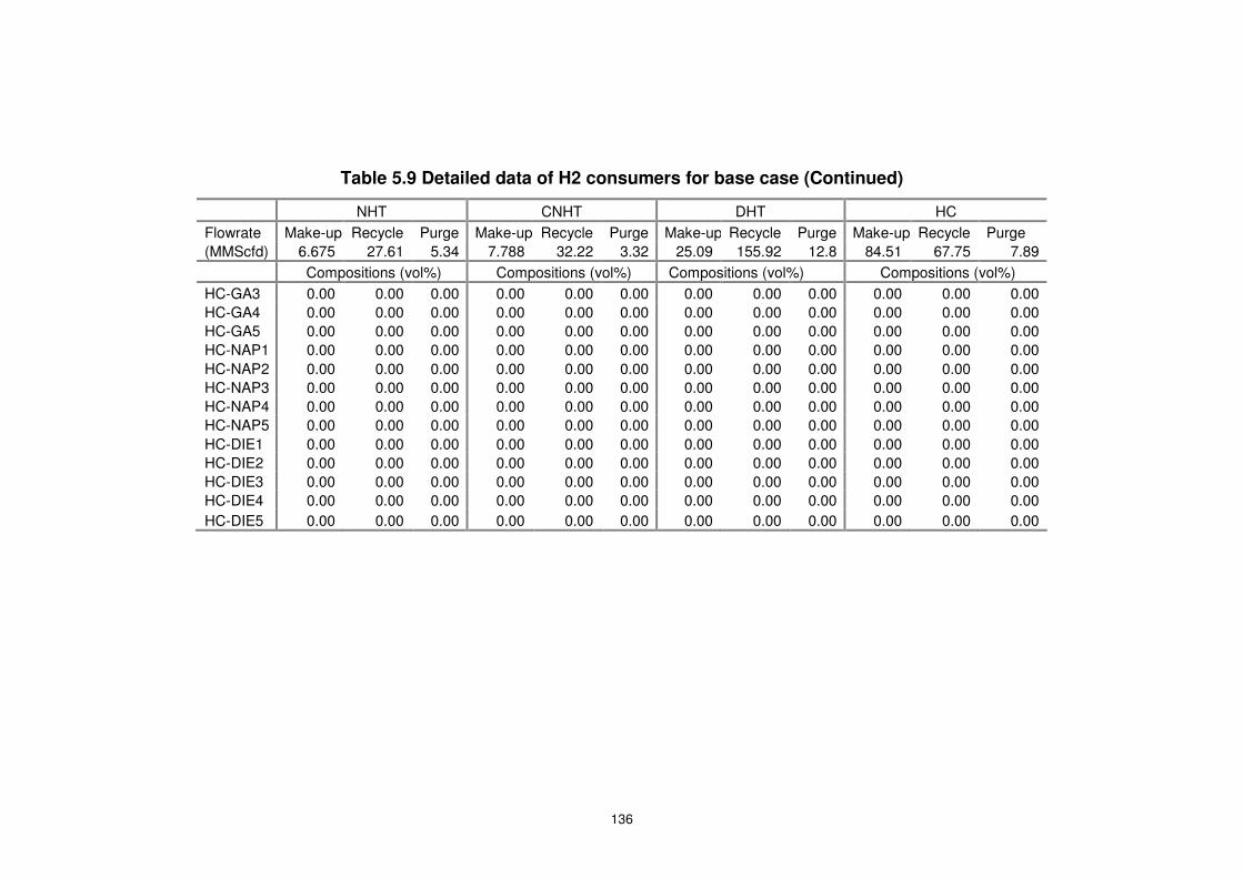
136
Table 5.9 Detailed data of H2 consumers for base case (Continued)
NHT CNHT DHT HC
Flowrate Make-up Recycle Purge Make-up Recycle Purge Make-up Recycle Purge Make-up Recycle Purge
(MMScfd) 6.675 27.61 5.34 7.788 32.22 3.32 25.09 155.92 12.8 84.51 67.75 7.89
Compositions (vol%) Compositions (vol%) Compositions (vol%) Compositions (vol%)
HC-GA3 0.00 0.00 0.00 0.00 0.00 0.00 0.00 0.00 0.00 0.00 0.00 0.00
HC-GA4 0.00 0.00 0.00 0.00 0.00 0.00 0.00 0.00 0.00 0.00 0.00 0.00
HC-GA5 0.00 0.00 0.00 0.00 0.00 0.00 0.00 0.00 0.00 0.00 0.00 0.00
HC-NAP1 0.00 0.00 0.00 0.00 0.00 0.00 0.00 0.00 0.00 0.00 0.00 0.00
HC-NAP2 0.00 0.00 0.00 0.00 0.00 0.00 0.00 0.00 0.00 0.00 0.00 0.00
HC-NAP3 0.00 0.00 0.00 0.00 0.00 0.00 0.00 0.00 0.00 0.00 0.00 0.00
HC-NAP4 0.00 0.00 0.00 0.00 0.00 0.00 0.00 0.00 0.00 0.00 0.00 0.00
HC-NAP5 0.00 0.00 0.00 0.00 0.00 0.00 0.00 0.00 0.00 0.00 0.00 0.00
HC-DIE1 0.00 0.00 0.00 0.00 0.00 0.00 0.00 0.00 0.00 0.00 0.00 0.00
HC-DIE2 0.00 0.00 0.00 0.00 0.00 0.00 0.00 0.00 0.00 0.00 0.00 0.00
HC-DIE3 0.00 0.00 0.00 0.00 0.00 0.00 0.00 0.00 0.00 0.00 0.00 0.00
HC-DIE4 0.00 0.00 0.00 0.00 0.00 0.00 0.00 0.00 0.00 0.00 0.00 0.00
HC-DIE5 0.00 0.00 0.00 0.00 0.00 0.00 0.00 0.00 0.00 0.00 0.00 0.00
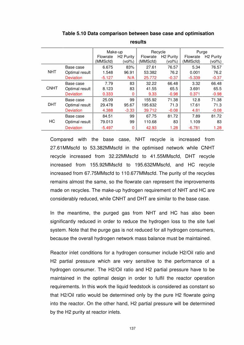
137
Table 5.10 Data comparison between base case and optimisation
results Make-up Recycle Purge Flowrate
(MMScfd) H2 Purity
(vol%) Flowrate
(MMScfd) H2 Purity
(vol%) Flowrate
(MMScfd) H2 Purity
(vol%)
Base case 6.675 83% 27.61 76.57 5.34 76.57
Optimal result 1.548 96.91 53.382 76.2 0.001 76.2 NHT
Deviation -5.127 N/A 25.772 -0.37 -5.339 -0.37
Base case 7.79 83 32.22 66.48 3.32 66.48
Optimal result 8.123 83 41.55 65.5 3.691 65.5 CNHT
Deviation 0.333 0 9.33 -0.98 0.371 -0.98
Base case 25.09 99 155.92 71.38 12.8 71.38
Optimal result 29.478 95.67 195.632 71.3 17.61 71.3 DHT
Deviation 4.388 -3.33 39.712 -0.08 4.81 -0.08
Base case 84.51 99 67.75 81.72 7.89 81.72
Optimal result 79.013 99 110.68 83 1.109 83 HC
Deviation -5.497 0 42.93 1.28 -6.781 1.28
Compared with the base case, NHT recycle is increased from
27.61MMscfd to 53.382MMscfd in the optimised network while CNHT
recycle increased from 32.22MMscfd to 41.55MMscfd, DHT recycle
increased from 155.92MMscfd to 195.632MMscfd, and HC recycle
increased from 67.75MMscfd to 110.677MMscfd. The purity of the recycles
remains almost the same, so the flowrate can represent the improvements
made on recycles. The make-up hydrogen requirement of NHT and HC are
considerably reduced, while CNHT and DHT are similar to the base case.
In the meantime, the purged gas from NHT and HC has also been
significantly reduced in order to reduce the hydrogen loss to the site fuel
system. Note that the purge gas is not reduced for all hydrogen consumers,
because the overall hydrogen network mass balance must be maintained.
Reactor inlet conditions for a hydrogen consumer include H2/Oil ratio and
H2 partial pressure which are very sensitive to the performance of a
hydrogen consumer. The H2/Oil ratio and H2 partial pressure have to be
maintained in the optimal design in order to fulfil the reactor operation
requirements. In this work the liquid feedstock is considered as constant so
that H2/Oil ratio would be determined only by the pure H2 flowrate going
into the reactor. On the other hand, H2 partial pressure will be determined
by the H2 purity at reactor inlets.
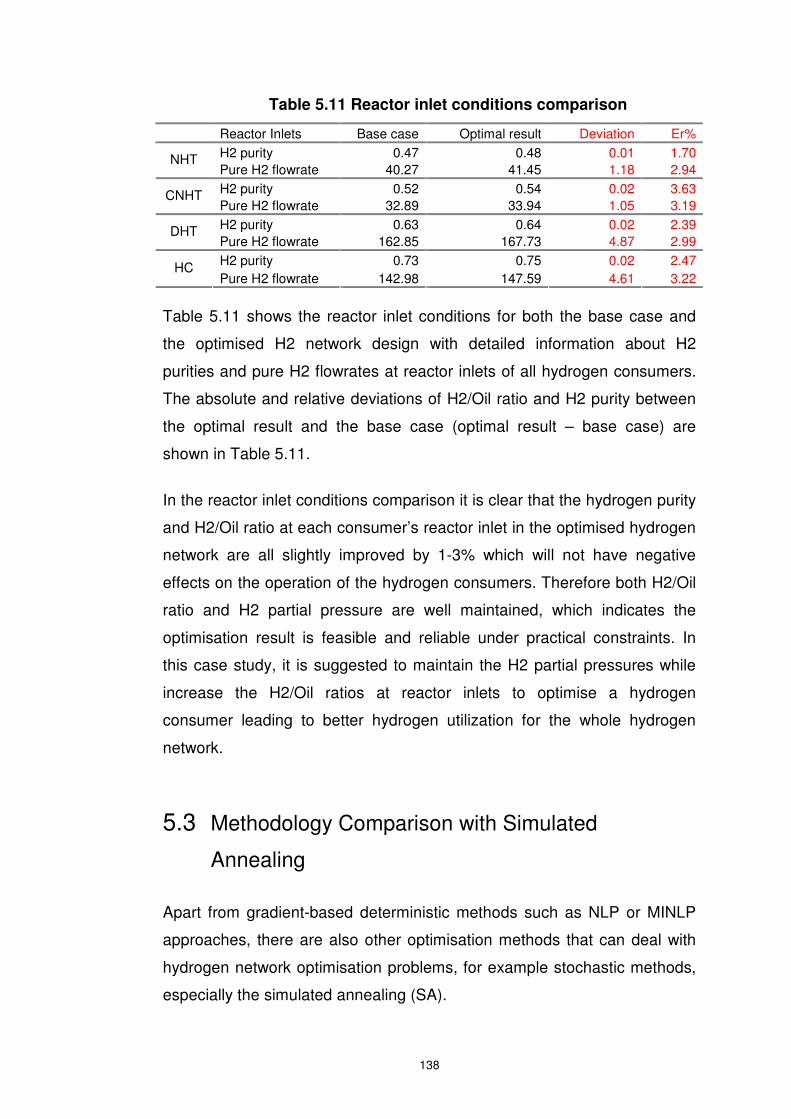
138
Table 5.11 Reactor inlet conditions comparison Reactor Inlets Base case Optimal result Deviation Er%
H2 purity 0.47 0.48 0.01 1.70 NHT
Pure H2 flowrate 40.27 41.45 1.18 2.94
H2 purity 0.52 0.54 0.02 3.63 CNHT
Pure H2 flowrate 32.89 33.94 1.05 3.19
H2 purity 0.63 0.64 0.02 2.39 DHT
Pure H2 flowrate 162.85 167.73 4.87 2.99
H2 purity 0.73 0.75 0.02 2.47 HC
Pure H2 flowrate 142.98 147.59 4.61 3.22
Table 5.11 shows the reactor inlet conditions for both the base case and
the optimised H2 network design with detailed information about H2
purities and pure H2 flowrates at reactor inlets of all hydrogen consumers.
The absolute and relative deviations of H2/Oil ratio and H2 purity between
the optimal result and the base case (optimal result – base case) are
shown in Table 5.11.
In the reactor inlet conditions comparison it is clear that the hydrogen purity
and H2/Oil ratio at each consumer’s reactor inlet in the optimised hydrogen
network are all slightly improved by 1-3% which will not have negative
effects on the operation of the hydrogen consumers. Therefore both H2/Oil
ratio and H2 partial pressure are well maintained, which indicates the
optimisation result is feasible and reliable under practical constraints. In
this case study, it is suggested to maintain the H2 partial pressures while
increase the H2/Oil ratios at reactor inlets to optimise a hydrogen
consumer leading to better hydrogen utilization for the whole hydrogen
network.
5.3 Methodology Comparison with Simulated
Annealing
Apart from gradient-based deterministic methods such as NLP or MINLP
approaches, there are also other optimisation methods that can deal with
hydrogen network optimisation problems, for example stochastic methods,
especially the simulated annealing (SA).

139
SA has been applied to solve optimisation problems such as heat
exchanger network design (Chen, 2007). Since the successful history has
proven the capability of SA in solving various optimisation problem, In 2009,
Loughrey has tried to use SA to optimise a refinery hydrogen network. In
this section, the SA hydrogen network optimisation is compared with NLP
hydrogen network optimisation to check for the performance differences of
these two methods when dealing with detailed hydrogen network
optimisation problems.
5.3.1 Brief Introduction of Simulated Annealing
The simulated annealing algorithm is known as a generic probabilistic
meta-algorithm for global optimisation problems. It is famous for its ability to
locate global or near-global optimum solution within large searching space.
Typically the simulated annealing method is used to solve non-convex,
integer involved or discrete optimisation problems to which gradient-based
methods such as NLP or MINLP are not effective. For most of integer
involved discrete optimisation problem, simulated annealing has proven its
considerable advantages compared with gradient-based approaches.
The name of SA comes from theory of annealing metallurgy, a technical
process that melts metal into crystal by using high initial temperature and
slow cooling procedure. During the melting process, atoms system would
become a disorder through all states of energy because of the heat. In the
following, controlled cooling method is required to slow down the cooling
procedure so that the system configuration with lower internal energy than
initial would be able to be achieved.The relationship between energy states
and temperatures can be expressed as the Boltzmann-Gibbs distribution:
=
aB
TenergyTc
xCP exp (5.8)
Where Penergy is the probability that a system is in a state x, CT is partition
function, x is energy state, CB is Boltzmann’s constant and Ta is
temperature.

140
As can be seen from Equation 5.8, the temperature would change with
energy states accordingly. In addition, at a higher temperature there will be
much higher probability for the system to be with a higher energy state,
resulting in higher mobility for atoms. Conversely, when the temperature
starts to decrease, the probability of the system with a high energy state
will be consistently reduced and if the cooling process is controlled slow
enough allowing the whole system to be in thermodynamic equilibrium at
any time approximately, the metal can be crystallized with minimum internal
energy. However, this kind of annealing technique requires rigorous
conditions for initial temperature and sufficiently slow cooling. Therefore,
failure of satisfying either condition can allow metal to be formed as glassy
meta-stable structure rather than wanted crystalline state.
By exploiting the metal annealing process, the idea of connecting this to
mathematical optimisation was first investigated by Kirkpatrick who
proposed analogies between physical annealing process and an
optimisation problem (Kirkpatrick, 1983). Then it was Spall that introduced
the general algorithm of SA as the first systematic SA method for
optimisation problems (Spall, 2003). By making use of a global parameter
to take control of the whole optimisation procedure, the proposed algorithm
is able to locate global optimum or near-global optimum solutions, which
has been convinced as the most advantages for SA against gradient-based
approaches. By taking not only improved objective values but also worse
objective values into account, the SA optimisation is able to overcome local
optimums with additional freedom to exploit a solution space.
5.3.2 SA Parameters
SA parameters are important because it will affect the problem solving
procedure sensitively. The selection of parameters can vary from problem
to problem. The most important parameters to be used in the hydrogen
network design problem are:
• Acceptance criteria

141
• Initial annealing temperature
• Cooling schedule
• Markov chain length
• Termination criteria
5.3.3 SA Moves
In the superstructure based optimisation algorithm, SA moves can be
extremely important as it will determine the scale of the searching space. In
the SA optimisation procedure, each move will introduce a new design and
the system will be changed therefore the moves for SA is very sensitive to
the optimisation and defining moves is quite important.
Figure 5.9 SA moves for hydrogen network optimisation
For a hydrogen network optimisation problem, the key consideration of
moves would be changes in flow which can be classified into two groups:
recycle flow change and flow between units change. The moves are made
based on random number generated and also affected by the probability
for each particular move. The move probabilities depend on the influence
factor of the variables. The higher the variable’s influence, the higher
probability of the move.
According to the complexity of the hydrogen network optimisation problem,
the move tree shown in Figure 5.9 can be extended to cover more
Hydrogen Network Move
Flow change
Recycle flow change
Flow between units change
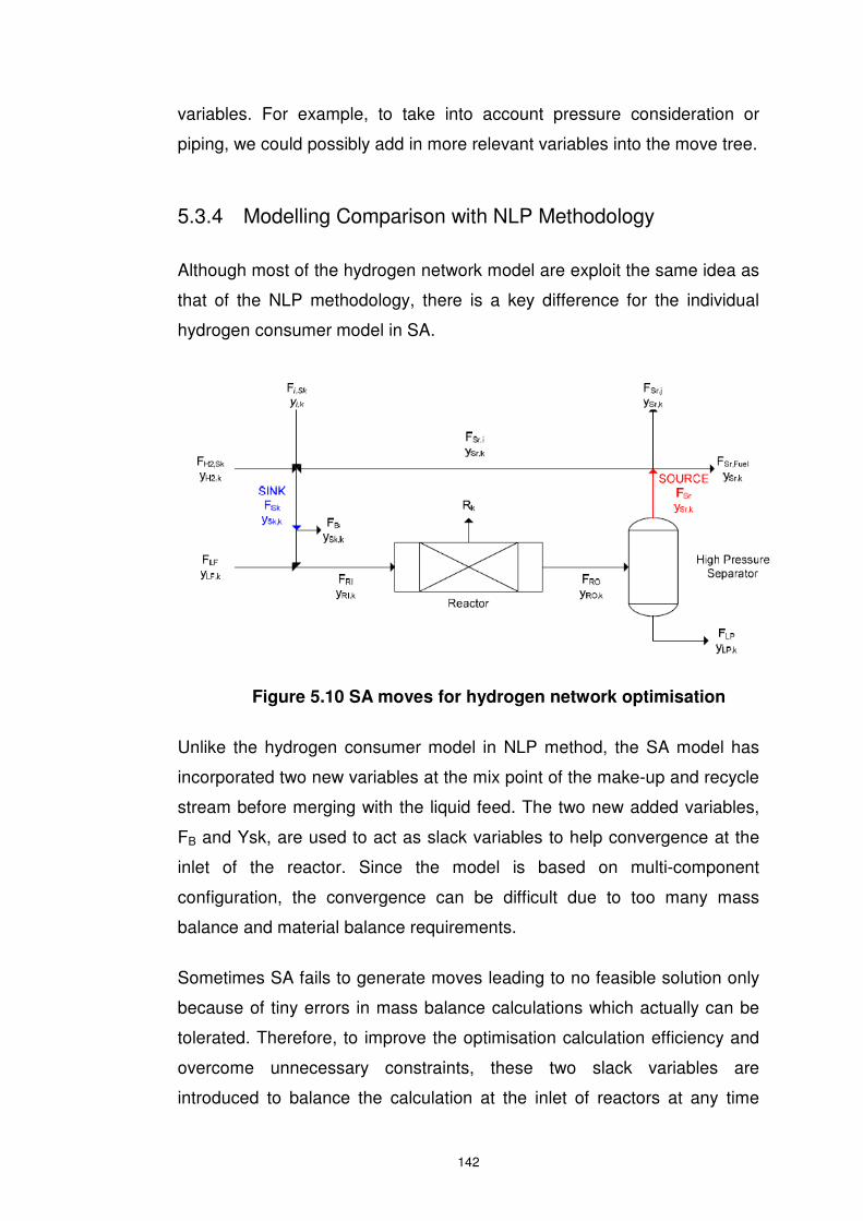
142
variables. For example, to take into account pressure consideration or
piping, we could possibly add in more relevant variables into the move tree.
5.3.4 Modelling Comparison with NLP Methodology
Although most of the hydrogen network model are exploit the same idea as
that of the NLP methodology, there is a key difference for the individual
hydrogen consumer model in SA.
Figure 5.10 SA moves for hydrogen network optimisation
Unlike the hydrogen consumer model in NLP method, the SA model has
incorporated two new variables at the mix point of the make-up and recycle
stream before merging with the liquid feed. The two new added variables,
FB and Ysk, are used to act as slack variables to help convergence at the
inlet of the reactor. Since the model is based on multi-component
configuration, the convergence can be difficult due to too many mass
balance and material balance requirements.
Sometimes SA fails to generate moves leading to no feasible solution only
because of tiny errors in mass balance calculations which actually can be
tolerated. Therefore, to improve the optimisation calculation efficiency and
overcome unnecessary constraints, these two slack variables are
introduced to balance the calculation at the inlet of reactors at any time

143
when required. To obtain a feasible solution, in the SA objective functions
all slack variables will be involved and minimized until the preset tolerance
is met. The hydrogen network distribution balance model and the super-
structure model adopted in SA are similar to the modelling used in the NLP
method.
5.3.5 Case Study Comparison
The base case that carried out for SA optimisation is exactly the same as
the one used in the NLP method as shown in Figure 5.5. In this four-
consumer hydrogen network system, 20 continuous manipulated variables
are involved with implementation of SA. The modelling and optimisation
are completed in MATLAB.
SA parameters have been set for optimisation. Table 5.12 shows all the
information about the SA parameters used in this hydrogen network
optimisation. The parameters for cooling rate and penalty are adjusted
slightly lower due to the problem complexity.
Table 5.12 SA parameters selection
Parameter Value
Initial temperature 1,000,000
Cooling rate 0.01
Markov chain length 30
Final temperature 0.0001
Move probability 50%
Penalty 0.001
As a stochastic algorithm, SA works much slower than NLP algorithms. For
this four-consumer hydrogen network optimisation problem, it normally
takes 10 – 11 hours to finish a scenario. Some key features are included in
this SA optimisation:

144
• Hydrogen pinch analysis
• Integrated Flash calculation
• Constant K-values strategy
Figure 5.11 SA optimisation solution
SA generates an optimised hydrogen network as shown in Figure 5.11.
Compared with the base case flowsheet, the optimisation result flowsheet
shows a much complicated configuration with 11 new connections between
hydrogen consumers.
Table 5.13 Network connections summary
NHT CNHT DHT HC Fuel
NHT 0 0 18.37 5.69 0
CNHT 0.51 0 0 0 11.75
DHT 12.92 0.24 0 67.75 11.19
HC 10.07 0.24 35.67 0 0

145
Table 5.13 gives a summary of the optimised hydrogen network
connections between processing units. The detailed data can be found in
table 5.14.
Table 5.14 Detailed data for SA optimal solution
NHT CNHT DHT HC
FH2 (MMscfd) 0.89 0.06 4.03 98.73 Hydrogen Plant
YH2 (vol%) 99.00 99.00 99.00 99.00
FH2 (MMscfd) 1.94 0.05 11.21 1.24 CCR YH2 (vol%) 83.00 83.00 83.00 83.00
FM (MMscfd) 26.33 17.52 69.31 121.95 Make-up YM (vol%) 76.51 74.26 78.13 94.31
Fr (MMscfd) 27.61 32.22 155.92 67.75 Recycle Yr (vol%) 76.57 66.48 71.38 81.72
FP (MMscfd) 24.51 12.31 57.15 46.00 Purge YP (vol%) 76.57 66.48 71.38 81.72
FSk (MMscfd) 53.93 49.67 225.11 189.69 Sink YSk (vol%) 76.79 68.34 74.51 89.68
FSr (MMscfd) 52.12 44.53 213.07 113.74 Source YSr (vol%) 76.57 66.48 71.38 81.72
In the optimum solution from SA, 6.18MMscfd hydrogen from the H2 plant
has been saved. The minimum hydrogen plant requirement is reduced from
109.6MMscfd to 103.7MMscfd. The SA hydrogen saving is almost the
same as the NLP optimisation.
Similarly as the NLP method, the optimisation result is compatible with the
minimum hydrogen target 102.4MMscfd given by the hydrogen pinch
analysis. This confirms that SA is able to optimise a multi-component
hydrogen network.
5.3.6 Methodology Comparisons
Taking into account all of the discussed aspects, we can summarise the
methodology comparisons between NLP and SA into Table 5.15.
From the result point of view, the two methods both performed well and
with almost the same optimum output. The NLP optimisation solution
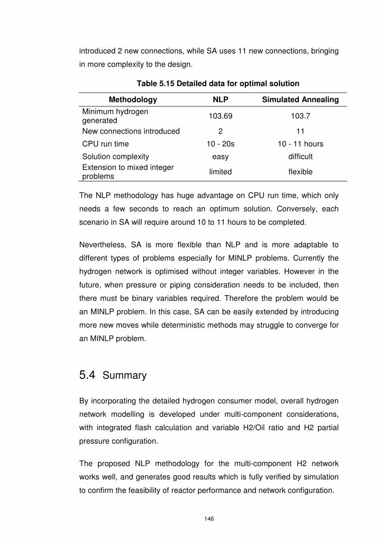
146
introduced 2 new connections, while SA uses 11 new connections, bringing
in more complexity to the design.
Table 5.15 Detailed data for optimal solution
Methodology NLP Simulated Annealing
Minimum hydrogen generated
103.69 103.7
New connections introduced 2 11
CPU run time 10 - 20s 10 - 11 hours
Solution complexity easy difficult
Extension to mixed integer problems
limited flexible
The NLP methodology has huge advantage on CPU run time, which only
needs a few seconds to reach an optimum solution. Conversely, each
scenario in SA will require around 10 to 11 hours to be completed.
Nevertheless, SA is more flexible than NLP and is more adaptable to
different types of problems especially for MINLP problems. Currently the
hydrogen network is optimised without integer variables. However in the
future, when pressure or piping consideration needs to be included, then
there must be binary variables required. Therefore the problem would be
an MINLP problem. In this case, SA can be easily extended by introducing
more new moves while deterministic methods may struggle to converge for
an MINLP problem.
5.4 Summary
By incorporating the detailed hydrogen consumer model, overall hydrogen
network modelling is developed under multi-component considerations,
with integrated flash calculation and variable H2/Oil ratio and H2 partial
pressure configuration.
The proposed NLP methodology for the multi-component H2 network
works well, and generates good results which is fully verified by simulation
to confirm the feasibility of reactor performance and network configuration.

147
In addition, the NLP is compared with SA as an optional optimisation
engine for the same case study. SA and NLP both work well with the multi-
component cases and generate good results. NLP optimisation is faster in
speed but with limited ability to cope with complicated problems, for
example MINLP problems. However, simulated annealing is much slower,
but with great flexibility for all kinds of problems and tends to produce near-
global optimum solutions. It can be concluded that the solver selection
should be dependent on the types of problems.

148
Chapter 6 Conclusions and Future work
6.1 Conclusions
In this thesis a few key improvements have been made to overcome the
drawbacks in existing methods. Firstly, a binary hydrogen network
optimisation methodology with variable H2 partial pressure and H2/Oil ratio
is proposed. Secondly, a detailed hydrogen consumer model is developed
under multi-component consideration. Finally, based on the proposed
detailed hydrogen consumer model, a multi-component hydrogen network
optimisation methodology is proposed.
For a binary component hydrogen network optimisation problem, H2/Oil
ratio and H2 partial pressure of each hydroprocessor can be slightly
relaxed to obtain extra flexibility. The variable H2/Oil ratio and H2 partial
pressure strategy has been proposed, verified, and tested with a industrial
case study in Chapter 3. This method is effective when dealing with over-
constrained network optimisation problems.
For hydroprocessor modelling, a detailed hydrogen consumer model has
been developed. To overcome the drawbacks of existing models, the
reaction modelling has incorporated light hydrocarbon production to obtain
a better reflection of the reality. Integrated flash calculation has been
introduced into a flash separator model for more efficient computation. By
combining the improved detailed hydrogen consumer models with a
hydrogen plant model and site fuel system, an overall hydrogen network
model can be constructed. By taking into account all of the improvements
discussed above, this model can be considered as the most detailed model
for hydrogen network optimisation so far.
On the basis of the detailed hydrogen network model, a multi-component
hydrogen network optimisation methodology is developed. A gradient-
based deterministic NLP solver is able to solve the network optimisation

149
problem and produce solutions efficiently. As another option, stochastic
simulated annealing was also tried to solve the same optimisation problem.
By comparing the two optimisation methods it is found out that each of
them has its advantages and disadvantages, and the methodology
selection should be dependent on the types of problems. Generally
deterministic methods are faster in computation, while stochastic methods
can be more effective when dealing with problems that contain many
discrete decisions.
6.2 Future Work
The current hydrogen network optimisation methodology is based on
single-period operation. However in a realistic refinery the operation is
always changing. Therefore the developed methodology should be
extended to multi-period hydrogen network operation.
Currently the performance of an individual hydrogen consumer model is
fixed by fixing the hydrogen consumption in reactors to simplify the H2
network optimisation problem. However the performance of a hydrogen
consumer can be improved by optimising the reactor inlet conditions. For
example, if the H2/Oil ratio or H2 partial pressure is increased the
hydrogen consumer could have better yield, better hydrodesulphurisation
and hydrodenitrogenation performance and also better olefins and
aromatics saturation, at the expense of more H2 consumption. Such trade-
offs are not included in the current hydrogen network optimisation
technology.
Using hydrogen more effectively rather than just saving H2 is the ultimate
goal of refinery hydrogen management, which can only be achieved by
proper integration between hydroprocessing reactions and hydrogen
networks.

150
Nomenclature
CMU Total power consumption of make-up hydrogen
compression of a consumer
CRE Power consumption of compressors of a consumer
Ef Compression efficiency
PCMU Power rate of make-up compressors of a consumer
PCRE Power rate of recycle compressors of a consumer
F Flowrates of a stream
Y compositions of a stream
FC Total reactor inlet flowrate of a consumer
FI Total flowrate of hydrogen producers
FIK Hydrogen flowrate from a producer to a purifier
FIJ Hydrogen flowrate from a producer to a consumer
FIN Hydrogen flowrate from a producer to a header
FJ Hydrogen flowrate from a consumer high pressure
purge to a consumer
FJK Hydrogen flowrate from a consumer high pressure
purge to a purifier
FJP Hydrogen flowrate from a consumer high pressure
purge to site fuel
FJL Hydrogen flowrate from a consumer low pressure
purge to a consumer
FJLK Hydrogen flowrate from a consumer low pressure
purge to a purifier
FJLN Hydrogen flowrate from a consumer low pressure
purge to a header
FJLP Hydrogen flowrate from a consumer low pressure
purge to site fuel
FJN Hydrogen flowrate from a consumer high pressure
purge to a header
FKJ Hydrogen flowrate from a purifier to a consumer
FKMAX Maximum limit of a purifier

151
FKN Hydrogen flowrate from a purifier to a header
FMUMAX Maximum limit of hydrogen make-up stream flowrate
FNJ Hydrogen flowrate from a header to a consumer
K Vapour liquid equilibrium (K-values)
YC Hydrogen purity at the reactor inlet of a consumer
YI Hydrogen purity of hydrogen produced from a
hydrogen producer
YJ Hydrogen purity of high pressure purge hydrogen of a
consumer
RECP Hydrogen recovery rate of a purifier
YJL Hydrogen purity of low pressure purge hydrogen of a a
consumer
YN Hydrogen purity of a header
YK Hydrogen purity of a purifier
Subscripts
feed Liquid feedstock
fi Flash inlet
H2C Hydrogen consumer
H2P Hydrogen producer
i A hydrogen producer (Chapter 3); a component
(Chapter 4 and 5)
imin Hydrogen production minimum limit of a producer
imax Hydrogen production maximum limit of a producer
j A hydrogen consumer
j1 Alias of subscript j
jmin Reactor inlet hydrogen minimum limit of a consumer
jmax Reactor inlet hydrogen maximum limit of a consumer
k A purifier (Chapter 3); A producer (Chapter 5)
Liq Liquid
mix Mix point
mu Make-up
n A header

152
pu Purge
re Recycle
ri Reactor inlet
SF Site fuel
U Unit price
vap Vapour
Superscripts
L Lower bound
U Upper bound
Abbreviations
ADU Atmospheric distillation unit
BFW Boiler feed water
CCR Catalytic reformer
CNHT Cracked naphtha hydrotreater
CRU Catalytic reformer unit
CW Cooling water
DCU Delayed coker unit
FCC Fluid catalytic cracker
GA Generic algorithm
HC Hydrocracker
HCU Hydrocracker unit
HDA Hydrodealkylation
HT Hydrotreater
LP Linear programming
KHT Kerosene hydrotreater
LPG Liquid petroleum gas
MILP Mixed integer linear programming
MINLP Mixed integer non-linear programming
NHT Naphtha hydrotreater
NLP Non-linear programming
OBJ Objective function

153
PSA Pressure swing adsorption
SA Simulated Annealing
VDU Vacuum distillation unit
VR Vacuum residue

154
References:
Abrardo, J. M., Khurana, V., Hydrogen Technologies to Meet Refiners’ Future
Needs, Hydrocarbon Processing, February 1995, 43-49
Ahmad, M.I., Zhang, N., and Megan, J., Modelling and Optimisation for Design of
Hydrogen Networks for Multi-period Operation. Journal of Cleaner Production18,
pp889-899, 2010
Aitani, A.M., Ali, S.A., Hydrogen Management in Modern Refineries, Erdol &
Knhle – Erdgas, January 1995
Alves, J.J., Analysis and Design of Refinery Hydrogen Distribution Systems. Ph.D.
thesis, Department of Process Integration, UMIST, Manchester, 1999
Alves, J.J., Towler, G.P., Analysis of Refinery Hydrogen Distribution Systems.
Industrial & Engineering Chemistry Research, 41, pp5759-5769, 2002
American Petroleum Institute. Technical Data Book-Petroleum Refining; 6th
Edition, Washington, D.C., 1997
Argaez, A. A.: Integrated Design of Water System, PhD thesis, Department of
Process Integration, UMIST, Manchester, U.K., February 1999
Armor, J. N.: Review – The multiple roles for catalysis in the production of H2,
Applied Catalysis A, General 176, pp159-176, 1999
Baird, C., Petroleum refining process correlations, HPI Consultants, Inc., 1999
Beychok, M., A Schematic Flow Diagram of a Typical Oil Refinery.
Wikipedia.org, 2008
http://en.wikipedia.org/wiki/Oil_refinery

155
Bressan, L., Collodi, G., Ruggeri, F., Hydrogen Generation for Modern Refineries.
Foster Wheeler Technical Paper, 2010
Brooke, A.; Kendrick, D.; Meeraus, A.: GAMS – A User’s Guide (Release 2.25),
GAMS Development Corporation, 1996
Campbell, D.M., Stochastic Modeling of Structure and Reaction in Hydrocarbon
Conversion, doctoral dissertation, University of Delaware, Newark, 1998
Chen, L., Heat-integrated Crude Oil Distillation System Design. Process
Integration Research Consortium, Manchester, 2007 (internal report)
Ding, Y., Feng X., Chu, K. H., Optimization of hydrogen distribution systems with
pressure constraints, Journal of Cleaner Production xxx (2010), in press and
available on line
Elshout, R., Hydrogen Production by Steam Reforming. Chemical Engineering,
May 2010
Environmental Protection Agency (EPA), Technical Amendments to the highway
and Nonroad Diesel Regulations, Direct Final Rule. Rules and Regulations, Vol 71,
No.83
Europa, Summaries of EU Legislation, Environment, Air Pollution, Sulphur
Content of Certain Liquid Fuels. 2007
http://europa.eu/legislation_summaries/environment/air_pollution/l21050_en.htm
Fonseca, A., Sa, V., Bento, H., Tavares, M. L.C., Pinto, G., Gomes, L.A.C.N.,
Hydrogen Distribution Network Optimization: a Refinery Case Study. Journal of
Cleaner Production, 16, pp1755-1763, 2008
Foo, D. C. Y., Manan, Z. A., Setting the Minimum Utility Gas Flowrate Targets
Using Cascade Analysis Technique. Industrial and Engineering Chemistry
Research, 45, pp5986-5995, 2006

156
Hallale, N., Liu, F., Refinery Hydrogen Management for Clean Fuels Production.
Advances in Environmental Research, 6, pp81-98, 2001
Hallale, N., Moore, I., Vauk, D., Hydrogen: Liability or Asset?. Chemical
Engineering Progress, 98 (9), pp66-75, 2002
Han, C. R., Hydrocracking Techniques and Engineering. 1st Edition, China
Petrochemical Press, Beijing, China, 2001 (in Chinese)
Hiller, M.H., Lascatena, J.J., Miller, G., Hydrogen for Hydroprocessing Operation,
presented at the 1987 NPRA Annual Meeting, March 1987, San Antionio, Texas,
U.S.
Refining Processes 2004, Hydrocarbon Processing® Magazine, 2004
IChemE., A Guide to Capital Cost Estimating, 3rd Edition, IChemE and The
Association of Cost Engineers, London, 1988
Johansen, T., Reghuraman, K.S., Hackett, L.A., Trends in Hydrogen Plant Design,
Hydrocarbon Processing, August 1992
Kemp, I.C., Pinch Analysis and Process Integration: A User Guide on Process
Integration for the Efficient Use of Energy. 2nd Edition, Elsevier Ltd, U.K., 2007
Khajehpour, M., Farhadi, F., Pishvaie, M.R., Reduced Superstructure Solution of
MINLP Problem in Refinery Hydrogen Management. International Journal of
Hydrogen Energy, 34, pp9233-9238, 2009
Korre, S. C., Neurock, M., Klein, M. T., Quann, R. J.: Hydrogenation of
polynuclear aromatic hydrocarbons. 2. Quantitative Structure/Reactivity
Correlations. Chemical Engineering Science 49: pp4191, 1994

157
Korre, S. C., Klein, M. T., Quann, R. J.: Polynuclear Aromatic Hydrocarbons
Hydrogenation. 1. Experimental Reaction Pathways and Kinetics. Industrial &
Engineering Chemistry Research 34: pp101-117, 1995
Kumar, A., Gautami, G., Khanam, S., Hydrogen Distribution in the Refinery Using
Mathematical Modelling. Journal of Energy, 35, pp3763-3772, 2010
Lamber, G.J., Schoeber, W.J.A.H., Helden, van H.J.A., The Hydrogen Balance in
Refineries, presented at Foster Wheeler Heavy Oil Processing and Hydrogen
Conference, April 1994, Noordwijk, Netherlands
Liao, Z., Wang, J., Yang, Y., Rong, G., Integrating Purifiers in Refinery Hydrogen
Networks: A Retrofit Case Study. Journal of Cleaner Production, 18, pp233–241,
2010
Linnhoff, B.: Pinch Analysis – A State-of-Art Overview, Trans IChemE, 71, Part
A, September 1993
Linnhoff, B., Mason, D.R., Wardle, I., Understanding Heat Exchanger Networks.
Computer and Chemical Engineering, 3, pp295, 1979
Liu, F., Hydrogen Integration in Oil Refineries. Ph.D. thesis, Department of
Process Integration, UMIST, U.K., Manchester, 2002
Liu, F., Zhang, N., Strategy of Purifier Selection and Integration in Hydrogen
Networks. Chemical Engineering Research and Design, 82, pp1315-1330, 2004
Lucas, A.G., Modern Petroleum Technology Volume 2 Downstream. John Wiley
& Sons, England, 2000
Malek, A., Farooq, S., Hydrogen Purification from Refinery Fuel Gas by Pressure
Swing Adsorption, AIChE Journal, 44, pp1985-1992, 1998
158
Meyers, R.A., Handbook of Petroleum Refining Processes Third Edition.
McGraw-Hill, U.S., 2003
Peng, B., Molecular Modelling of Refinery Processes. PhD Thesis, Department of
Process Integration, UMIST, Manchester, 1999
Peramanu, S., Cox, B.G., Pruden, B.B., Economics of Hydrogen Recovery
Processes for the Purification of Hydroprocessor Purge and Off-gases.
International Journal of Hydrogen Energy, 24, pp405-424, 1999
Pacalowska, B., Whysall, M., Narasimhan, M.V., Improve Hydrogen Recovery
from Refinery Off-gases, Hydrocarbon Processing, pp55-59, November 1996
Phillips, G., Hydrogen – innovative Business Solutions for 2005 & beyond,
presented on the European Refining Technology Conference – Process, Paris,
France November 1999
Rajesh, J.K., Gupta, S.K., Rangaiah, G.P., Ray, A.K., Multiobjective Optimization
of Steam Reformer Performance Using Genetic Algorithm, Industrial &
Engineering Chemical Research, 39, pp706-717, 2000
Ramachandran, R., Menon, R.K., An Overview of Industrial Uses of Hydrogen.
International Journal of Hydrogen Energy, 23, pp593-598, 1998
Ratan, S., Hydrogen Management System, KTI Newsletter, pp24-32, Fall 1994
Reid, R.C., Prausnitz, J.M., Poling, B.E., The Properties of Gases and Liquids. 4th
Edition, McGraw-Hill, 1987
Simpson, D.M., Hydrogen Management in a Synthetic Crude Refinery.
International Journal of Hydrogen Energy, 9, pp95-99, 1984
159
Singh, B. B., Bi-linear Data Reconciliation and Rigorous Optimisation of Refinery
Hydrogen Networks with Hydrogen Plant. Process Integration Research
Consortium, Manchester, 2006
Smith, R., Chemical Process Design and Integration. John Wiley & Sons, U.K.,
2005
Smith, W.N., Santangelo, J.G., Hydrogen: Production and Marketing, ACS
Symposium Series 116, American Chemical Society, Washington, D.C., 1980
Sun, J., Molecular Modelling and Integration Analysis of Hydroprocessors. PhD
Thesis, University of Manchester, U.K., Manchester, 2004
Swain, E.J., U.S. Crude Slate Continues to Get Heavier, Higher in Sulphur, Oil &
Gas Journal, pp37-42, January 9 1995
Towler, G.P., Mann R., Serriere, A.J., Gabaude, C.M.D., Refinery Hydrogen
Management: Cost Analysis of Chemically Integrated Facilities. Industrial and
Engineering Chemistry Research, 35, pp2378-2388, 1996
Uppaluri, R., Synthesis of Membrane Systems, presented at Process Integration
Research Consortium Meeting, October, 2000, Manchester
U.S. Energy Information Administration., U.S. Sulfur Content (Weighted Average)
of Crude Oil Input to Refineries, July 2010
http://tonto.eia.doe.gov/dnav/pet/hist/LeafHandler.ashx?n=pet&s=mcrs1us2&f=a
Vervalin, C.H., Gas Processing Handbook, Hydrocarbon Processing, 73 (4), 1994
Warmuzinski, K., Tanczyk, M., Multicomponent Pressure Swing Adsorption Part I.
Modelling of Large-scale PSA Installation, Chemical Engineering and Processing
36, pp89-99, 1997

160
Zhang, N., Singh, B.B., Liu, F., A Systematic Approach for Refinery Hydrogen
Network Management. PRES2008, Prague, Czech Republic, 2008
Zhao, Z., Liu, G., Feng, X., the Integration of the Hydrogen Distribution System
with Multiple Impurities. Chemical Engineering Research and Design, 85, pp1295-
1304, 2007

161
Appendix A Binary H2 network optimisation
program codes (GAMS)
option NLP=minos5; Set i H2 producers/HP1, HP2, HP3, HP4 / j H2 consumers/HC1, HC2, HT1, HT2, HT3, HT4, HT5, HT6, HT7/ k Purifiers/PSA, MEM/ n H2 mains/12Bar, 24Bar/ ; Alias (j, j1); Parameters FH2S(i) H2 producer flow Nm3h-1/ HP1 60000 HP2 10000 HP3 167391 HP4 35720 / YH2S(i) H2 producer purity/ HP1 91.59 HP2 91.59 HP3 99.9 HP4 92 / PH2S(i) H2 producer pressure MPa/ HP1 1.3 HP2 1.7 HP3 2.4 HP4 2.8 / CH2S(i) H2 producer price RMB.Nm3-1/ HP1 1.118297505 HP2 1.118289637 HP3 1.220978826 HP4 1.123301936 / FH2C(j) H2 consumer reactor inlet flow Nm3h-1/ HC1 158931

162
HC2 501616 HT1 109728 HT2 126995 HT3 3237 HT4 298 HT5 408747 HT6 154944 HT7 11733 / YH2C(j) H2 consumer reactor inlet purity/ HC1 84.22 HC2 94.89 HT1 87.11 HT2 84.46 HT3 92 HT4 91 HT5 94.19 HT6 81.22 HT7 88.29 / PH2C(j) H2 consumer reactor inlet pressure MPa/ HC1 17.5 HC2 17.5 HT1 4.6 HT2 7 HT3 2.5 HT4 5.3 HT5 16.4 HT6 11.5 HT7 6.5 / FH2V(j) H2 consumer high pressure flash vapor flow Nm3h-1/ HC1 125354 HC2 407628 HT1 96609 HT2 95246 HT3 0 HT4 0 HT5 359250 HT6 123433 HT7 8762 / YH2V(j) H2 consumer high pressure flash vapor purity/ HC1 81.57

163
HC2 93.73 HT1 85.5 HT2 82.2 HT3 91 HT4 91 HT5 93.4 HT6 76.45 HT7 85.4u / PH2V(j) H2 consumer high pressure flash vapor pressure MPa/ HC1 15.6 HC2 15.6 HT1 3.9 HT2 6.5 HT3 1.5 HT4 5.3 HT5 15.6 HT6 10 HT7 6 / FH2L(j) H2 consumer low pressure purge flow Nm3h-1/ HC1 2462 HC2 7440 HT1 954 HT2 4445 HT3 0 HT4 0 HT5 7000 HT6 2165 HT7 686 / YH2L(j) H2 consumer low pressure purge purity/ HC1 70.0 HC2 85.32 HT1 67.25 HT2 56.58 HT3 70 HT4 70 HT5 90.0 HT6 66.29 HT7 68 /

164
PH2L(j) H2 consumer low pressure purge pressure MPa/ HC1 1.95 HC2 1.95 HT1 1.2 HT2 1.5 HT3 0 HT4 0.45 HT5 2.1 HT6 2.5 HT7 1.4 / PCMUI(j) Inlet pressure of make-up compressors of hydrogen consumers/ HC1 1.1 HC2 1.1 HT1 1.15 HT2 1.2 HT3 2.5 HT4 1.2 HT5 2.2 HT6 2.2 HT7 1.2 / PCMUO(j) Outlet pressure of make-up compressors of hydrogen consumers/ HC1 18.1 HC2 18.1 HT1 5.8 HT2 7.8 HT3 2.5 HT4 6.5 HT5 17.35 HT6 11.9 HT7 7.3 / PCREI(j) Inlet pressure of recycle compressors of hydrogen consumers/ HC1 15.6 HC2 15.6 HT1 3.9 HT2 6.5 HT3 0 HT4 0 HT5 15.5 HT6 9.9 HT7 5.8

165
/ PCREO(j) Outlet pressure of recycle compressors of hydrogen consumers/ HC1 18.1 HC2 18.1 HT1 5.8 HT2 7.8 HT3 0 HT4 0 HT5 17.35 HT6 11.9 HT7 7 / PPO(k) Purification outlet pressure MPa/ PSA 2.4 MEM 1.2 / RECP(k) Purification recovery/ PSA 0.9 MEM 0.9 / YH2P(k) Purity of H2 purification/ PSA 99.9 MEM 89 / Pmax(k) Purification max flow/ PSA 60000 MEM 10000 / FH2Smax(i) H2 producer max flow Nm3h-1/ HP1 50700 HP2 15000 HP3 60000 HP4 29500 / FH2Smin(i) H2 producer min flow Nm3h-1/ HP1 50700 HP2 15000 HP3 0 HP4 29500 /

166
CMUmax(j) Maximum make-up flow of hydrogen consumers Nm3/ HC1 48000 HC2 110000 HT1 16000 HT2 42017 HT3 7000 HT4 4000 HT5 60602 HT6 44000 HT7 9001 / PPCMU(j) Power rate of make-up compressors of hydrogen consumers kW.Nm3-1/ HC1 0.1333 HC2 0.1149 HT1 0.07 HT2 0.09524 HT3 0 HT4 0.0875 HT5 0.1096 HT6 0.0971 HT7 0.1111 / PPCRE(j) Power rate of recycle compressors of hydrogen consumers kW.Nm3-1/ HC1 0.0103 HC2 0.01003 HT1 0.019 HT2 0.0117 HT3 0 HT4 0 HT5 0.0129 HT6 0.01043 HT7 0.0154 / PH2M(n) Pressure of H2 mains MPa/ 12Bar 1.2 24Bar 2.4 / ; Variables FH2 Total H2 production Nm3.hr-1 Cost Total H2 production cost RMB

167
; Positive variables FI(i) Total flowrate of producer i Nm3.h-1 FIJ(i,j) Flowrate from producer i to consumer j Nm3.h-1 FIK(i,k) Flowrate from producer i to purifier k Nm3.h-1 FIN(i,n) Flowrate from producer i to H2 main n Nm3.h-1 FNJ(n,j) Flowrate from H2 main n to consumer j Nm3.h-1 FJ(j,j1) Flowrate from consumer j to consumer j1 Nm3.h-1 FJN(j,n) Flowrate from consumer j to H2 main n Nm3.h-1 FJK(j,k) Flowrate from consumer j to purifier k Nm3.h-1 FJL(j,j1) Flowrate from low pressure flash of consumer j to consumer j1 Nm3.h-1 FJNL(j,n) Flowrate from low pressure flash of consumer j to H2 main n Nm3.h-1 FJKL(j,k) Flowrate from low pressure flash of consumer j to purifier k Nm3.h-1 FKJ(k,j) Flowrate of purifier k to consumer j Nm3.h-1 FKN(k,n) Flowrate of purifier k to H2 main n Nm3.h-1 FPH(j) Flowrate of high pressure H2 purge from consumer j Nm3.h-1 FPL(j) Flowrate of low pressure H2 purge from consumer j Nm3.h-1 YN(n) Purity of H2 main n CMU(j) Power cost of make-up compressors CRE(j) Power cost of recycle compressors ; Equations MFI(i) Mass balance of H2 producer i MaxFI(i) Maximum flow of producer i MinFI(i) Minimum flow of producer i MFN(n) Mass balance of H2 main n MHN(n) H2 balance of H2 main n *MFJR(j) Mass balance of consumer j reactor inlet MHJR(j) H2 balance of consumer j reactor inlet MFJF(j) Mass balance of consumer j high pressure flash MFJL(j) Mass balance of consumer j low pressure purge MFK(k) Mass balance of purifier k FPmax(k) Max. flowrate of purifier products FMUmax(j) Max. flowrate of make-up flows CCMU(j) Power cost of make-up compressors CCRE(j) Power cost of recycle compressors OBJ Objective function ; MFI(i).. FI(i) =e= sum(j, FIJ(i,j))+sum(n, FIN(i,n))+sum(k, FIK(i,k)); MaxFI(i).. FI(i) =l= FH2Smax(i); MinFI(i).. FI(i) =g= FH2Smin(i); MFN(n).. sum(i, FIN(i,n))+sum(j, FJN(j,n)+FJNL(j,n))+sum(k, FKN(k,n)) =e= sum(j, FNJ(n,j));

168
MHN(n).. sum(i,FIN(i,n)*YH2S(i))+sum(j,FJN(j,n)*YH2V(j) +FJNL(j,n)*YH2L(j))+sum(k, FKN(k,n)*YH2P(k)) =e= sum(j, FNJ(n,j)*YN(n)); MHJR(j).. FH2C(j)*YH2C(j) =e= sum(i, FIJ(i,j)*YH2S(i))+sum(j1, FJ(j1,j)*YH2V(j1)+FJL(j1,j)*YH2L(j1))+sum(k, FKJ(k,j)*YH2P(k)) + sum(n, FNJ(n,j)*YN(n)); MFJF(j).. FH2V(j) =e= sum(j1, FJ(j,j1))+sum(k, FJK(j,k))+sum(n, FJN(j,n))+FPH(j); MFJL(j).. FH2L(j) =e= sum(j1, FJL(j,j1))+sum(k, FJKL(j,k))+sum(n, FJNL(j,n))+FPL(j); MFK(k).. (sum(j, FJK(j,k)*YH2V(j)+FJKL(j,k)*YH2L(j))+sum(i, FIK(i,k)*YH2S(i)))*RECP(k) =e= (sum(j, FKJ(k,j))+sum(n, FKN(k,n)))*YH2P(k); FPmax(k).. (sum(j, FKJ(k,j))+sum(n, FKN(k,n))) =l= Pmax(k); FMUmax(j).. FH2C(j) - FJ(j,j) =l= CMUmax(j); CCMU(j).. CMU(j) =e= 0.6*PPCMU(j)*(sum(i, FIJ(i,j))+sum(j1$(ord(j1) ne ord(j)), FJ(j1,j))+sum(k, FKJ(k,j))+sum(n, FNJ(n,j))+sum(j1, FJL(j1,j))); CCRE(j).. CRE(j) =e= 0.6*PPCRE(j)*FJ(j,j); OBJ.. FH2 =e= sum(i, FI(i)*CH2S(i))-sum(j, FPH(j)*(0.5720631*YH2V(j)+1.78571232*(100-YH2V(j))) +FPL(j)*(0.5720631*YH2L(j)+1.78571232*(100-YH2L(j))))/100 - sum(k, sum(j,(FJK(j,k)*YH2V(j)+FJKL(j,k)*YH2L(j)) +sum(i, FIK(i,k)*YH2S(i)))*(1-RECP(k))*0.5720631/100) - (sum((j,k),FJK(j,k)+FJKL(j,k))+sum((i,k), FIK(i,k))- (sum((i,k), FIK(i,k)*YH2S(i)/100) +sum((j,k), (FJK(j,k)*YH2V(j)+FJKL(j,k)*YH2L(j))/100)))*1.78571232 + sum(j, CMU(j)+CRE(j)); model M /all/; FIJ.fx('HP3',j) =0; FIJ.fx('HP1',j) =0; FIJ.fx(' HP2',j) =0; FIN.fx('HP3','12Bar') =0; FIN.fx(' HP4','12Bar') =0; FIJ.fx(' HP4',j) =0; FJ.fx(j,j1)$(ord(j) ne ord(j1)) = 0; FNJ.fx('12Bar',' HT6 ') =0; FNJ.fx('12Bar',' HT5') =0;

169
FNJ.fx('12Bar','HC2') =0; FNJ.fx('24Bar','HC1') =0; FNJ.fx('24Bar','HT7') =0; FNJ.fx('24Bar','HT1') =0; FNJ.fx('24Bar','HT2') =0; FNJ.fx('24Bar','HT4') =0; FNJ.fx('24Bar','HT7') =0; FJK.fx(j,k) =0; FJKL.fx(j,'MEM') =0; FJN.fx(j,'24Bar') =0; FIN.fx('HP1','24Bar') =0; FIN.fx(' HP2','24Bar') =0; FJNL.fx(j,'24Bar') =0; FPH.fx(j) =0; FJL.fx(j,j1) =0; FKJ.fx('PSA','HC2') =0; FKJ.fx('PSA',' HT6 ') =0; FKJ.fx('PSA',' HT5') =0; FKN.fx('PSA','12Bar') =0; FIK.fx(i,k)$(ord(i) ne 6) =0; *FIK.fx(i,k) =0; *FI.fx('HP3') = 22800; Solve M using NLP minimizing FH2; Solve M using NLP minimizing FH2; *Solve M using NLP minimizing FH2; *Solve M using NLP minimizing FH2; *Solve M using NLP minimizing FH2; *Solve M using NLP minimizing FH2; display FI.l, FIJ.l, FIK.l, FIN.l, FJ.l, FJL.l, FNJ.l, FJK.l, FJKL.l, FKN.l, YN.l, FKJ.l, FJN.l, FJNL.l, FPH.l, FPL.l; parameter YH2CC(j) Calculated reactor inlet purities; YH2CC(j) = (sum(i, FIJ.l(i,j)*YH2S(i))+sum(j1, FJ.l(j1,j)*YH2V(j1)+ FJL.l(j1,j)*YH2L(j1))+sum(k, FKJ.l(k,j)*YH2P(k)) + sum(n, FNJ.l(n,j)*YN.l(n)))/ (sum(i, FIJ.l(i,j))+sum(j1, FJ.l(j1,j)+FJL.l(j1,j))+sum(k, FKJ.l(k,j)) + sum(n, FNJ.l(n,j)));

170
parameter FH2CC(j) Calculated reactor inlet flows; FH2CC(j) = sum(i, FIJ.l(i,j))+sum(j1, FJ.l(j1,j)+FJL.l(j1,j))+sum(k, FKJ.l(k,j)) + sum(n, FNJ.l(n,j)); parameter FPSA PSA feed flowrate; FPSA = sum(j, FJK.l(j,'PSA'))+ sum(j,FJKL.l(j,'PSA'))+sum(i, FIK.l(i,'PSA')); parameter YRPSA PSA residue purity; YRPSA = (sum(j, FJK.l(j,'PSA')*YH2V(j))+ sum(j,FJKL.l(j,'PSA')*YH2L(j))+sum(i, FIK.l(i,'PSA')*YH2S(i)) -sum(j, FKJ.l('PSA',j)*99.9))/(FPSA-sum(j, FKJ.l('PSA',j))); parameter CPC Compression cost; CPC = sum(j, CMU.l(j)+CRE.l(j)) display YH2CC, YH2C, FH2C, FH2CC, FPSA, YRPSA, CPC, FH2.l;
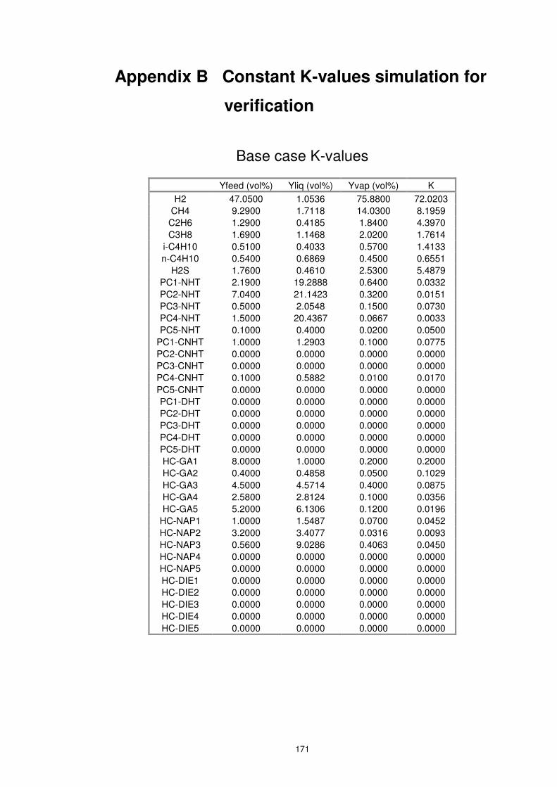
171
Appendix B Constant K-values simulation for
verification
Base case K-values
Yfeed (vol%) Yliq (vol%) Yvap (vol%) K
H2 47.0500 1.0536 75.8800 72.0203
CH4 9.2900 1.7118 14.0300 8.1959
C2H6 1.2900 0.4185 1.8400 4.3970
C3H8 1.6900 1.1468 2.0200 1.7614
i-C4H10 0.5100 0.4033 0.5700 1.4133
n-C4H10 0.5400 0.6869 0.4500 0.6551
H2S 1.7600 0.4610 2.5300 5.4879
PC1-NHT 2.1900 19.2888 0.6400 0.0332
PC2-NHT 7.0400 21.1423 0.3200 0.0151
PC3-NHT 0.5000 2.0548 0.1500 0.0730
PC4-NHT 1.5000 20.4367 0.0667 0.0033
PC5-NHT 0.1000 0.4000 0.0200 0.0500
PC1-CNHT 1.0000 1.2903 0.1000 0.0775
PC2-CNHT 0.0000 0.0000 0.0000 0.0000
PC3-CNHT 0.0000 0.0000 0.0000 0.0000
PC4-CNHT 0.1000 0.5882 0.0100 0.0170
PC5-CNHT 0.0000 0.0000 0.0000 0.0000
PC1-DHT 0.0000 0.0000 0.0000 0.0000
PC2-DHT 0.0000 0.0000 0.0000 0.0000
PC3-DHT 0.0000 0.0000 0.0000 0.0000
PC4-DHT 0.0000 0.0000 0.0000 0.0000
PC5-DHT 0.0000 0.0000 0.0000 0.0000
HC-GA1 8.0000 1.0000 0.2000 0.2000
HC-GA2 0.4000 0.4858 0.0500 0.1029
HC-GA3 4.5000 4.5714 0.4000 0.0875
HC-GA4 2.5800 2.8124 0.1000 0.0356
HC-GA5 5.2000 6.1306 0.1200 0.0196
HC-NAP1 1.0000 1.5487 0.0700 0.0452
HC-NAP2 3.2000 3.4077 0.0316 0.0093
HC-NAP3 0.5600 9.0286 0.4063 0.0450
HC-NAP4 0.0000 0.0000 0.0000 0.0000
HC-NAP5 0.0000 0.0000 0.0000 0.0000
HC-DIE1 0.0000 0.0000 0.0000 0.0000
HC-DIE2 0.0000 0.0000 0.0000 0.0000
HC-DIE3 0.0000 0.0000 0.0000 0.0000
HC-DIE4 0.0000 0.0000 0.0000 0.0000
HC-DIE5 0.0000 0.0000 0.0000 0.0000

172
Simulation Scenario 1
Yfeed (vol%) Yliq (vol%) Yvap (vol%) K
H2 51.0500 1.1100 82.3500 73.9495
CH4 7.9500 1.6700 11.8800 7.1032
C2H6 1.1900 0.4100 1.6800 4.1215
C3H8 1.6800 1.5100 1.7800 1.1787
i-C4H10 0.6300 0.5200 0.6900 1.3166
n-C4H10 0.5800 0.6900 0.5100 0.7301
H2S 1.7600 0.6100 2.4700 4.0561
PC1-NHT 2.4500 25.6800 0.7004 0.0273
PC2-NHT 12.0000 15.2300 0.1747 0.0115
PC3-NHT 1.1000 12.0000 0.0611 0.0051
PC4-NHT 0.4500 0.5000 0.0010 0.0020
PC5-NHT 0.5000 5.6900 0.0048 0.0008
PC1-CNHT 0.2000 1.0000 0.0225 0.0225
PC2-CNHT 0.0000 0.0000 0.0000 0.0000
PC3-CNHT 0.0000 0.0000 0.0000 0.0000
PC4-CNHT 0.3700 0.5000 0.0004 0.0007
PC5-CNHT 0.0000 0.0000 0.0000 0.0000
PC1-DHT 0.0000 1.1100 82.3500 0.0000
PC2-DHT 0.0000 1.1100 82.3500 0.0000
PC3-DHT 0.0000 1.1100 82.3500 0.0000
PC4-DHT 0.0000 1.1100 82.3500 0.0000
PC5-DHT 0.0000 1.1100 82.3500 0.0000
HC-GA1 5.1500 10.0000 1.7734 0.1773
HC-GA2 3.5600 5.6800 0.5845 0.1029
HC-GA3 0.3200 0.5600 0.0346 0.0617
HC-GA4 2.2000 5.1200 0.1821 0.0356
HC-GA5 3.1200 5.5100 0.1079 0.0196
HC-NAP1 3.0400 4.2500 0.0981 0.0231
HC-NAP2 0.5800 1.2000 0.0111 0.0093
HC-NAP3 0.1200 0.5600 0.0020 0.0035
HC-NAP4 0.0000 0.0000 0.0000 0.0000
HC-NAP5 0.0000 0.0000 0.0000 0.0000
HC-DIE1 0.0000 0.0000 0.0000 0.0000
HC-DIE2 0.0000 0.0000 0.0000 0.0000
HC-DIE3 0.0000 0.0000 0.0000 0.0000
HC-DIE4 0.0000 0.0000 0.0000 0.0000
HC-DIE5 0.0000 0.0000 0.0000 0.0000

173
Simulation Scenario 2
Yfeed (vol%) Yliq (vol%) Yvap (vol%) K
H2 49.0500 1.0800 79.1200 73.0116
CH4 8.0100 1.7000 11.9500 7.0208
C2H6 1.2400 0.4400 1.7400 3.9813
C3H8 1.7000 1.5200 1.8000 1.1882
i-C4H10 0.6200 0.5100 0.6900 1.3388
n-C4H10 0.5600 0.6900 0.4700 0.6833
H2S 1.7700 0.5600 2.5200 4.5042
PC1-NHT 11.5100 25.6800 1.9993 0.0779
PC2-NHT 11.1800 24.4500 2.0428 0.0835
PC3-NHT 11.6200 23.5400 1.8770 0.0797
PC4-NHT 2.0000 8.5600 0.7417 0.0867
PC5-NHT 0.7400 11.3700 0.4755 0.0418
PC1-CNHT 0.0000 0.0000 0.0000 0.0000
PC2-CNHT 0.0000 0.0000 0.0000 0.0000
PC3-CNHT 0.0000 0.0000 0.0000 0.0000
PC4-CNHT 0.0000 0.0000 0.0000 0.0000
PC5-CNHT 0.0000 0.0000 0.0000 0.0000
PC1-DHT 0.0000 0.0000 0.0000 0.0000
PC2-DHT 0.0000 0.0000 0.0000 0.0000
PC3-DHT 0.0000 0.0000 0.0000 0.0000
PC4-DHT 0.0000 0.0000 0.0000 0.0000
PC5-DHT 0.0000 1.0800 79.1200 0.0000
HC-GA1 0.0000 0.0000 0.0000 0.0000
HC-GA2 0.0000 0.0000 0.0000 0.0000
HC-GA3 0.0000 0.0000 0.0000 0.0000
HC-GA4 0.0000 0.0000 0.0000 0.0000
HC-GA5 0.0000 0.0000 0.0000 0.0000
HC-NAP1 0.0000 0.0000 0.0000 0.0000
HC-NAP2 0.0000 0.0000 0.0000 0.0000
HC-NAP3 0.0000 0.0000 0.0000 0.0000
HC-NAP4 0.0000 0.0000 0.0000 0.0000
HC-NAP5 0.0000 0.0000 0.0000 0.0000
HC-DIE1 0.0000 0.0000 0.0000 0.0000
HC-DIE2 0.0000 0.0000 0.0000 0.0000
HC-DIE3 0.0000 0.0000 0.0000 0.0000
HC-DIE4 0.0000 0.0000 0.0000 0.0000
HC-DIE5 0.0000 0.0000 0.0000 0.0000

174
Simulation Scenario 3
Yfeed (vol%) Yliq (vol%) Yvap (vol%) K
H2 45.0500 1.0200 72.6400 71.2198
CH4 11.0000 2.0000 16.6200 8.3037
C2H6 2.3000 1.0200 3.1000 3.0445
C3H8 1.7300 1.1600 2.0700 1.7803
i-C4H10 0.7100 0.6500 0.7400 1.1359
n-C4H10 0.6900 0.8000 0.6200 0.7658
H2S 1.1200 2.5600 2.8200 5.0231
PC1-NHT 1.4500 2.5800 0.0856 0.0332
PC2-NHT 5.6900 15.2000 0.2301 0.0151
PC3-NHT 0.0900 0.5000 0.0037 0.0073
PC4-NHT 3.2600 10.9900 0.0359 0.0033
PC5-NHT 2.5600 9.2300 0.0138 0.0015
PC1-CNHT 5.4200 8.2400 0.1855 0.0225
PC2-CNHT 5.5500 7.5600 0.0645 0.0085
PC3-CNHT 0.5700 1.0700 0.0025 0.0023
PC4-CNHT 0.6200 1.2300 0.0009 0.0007
PC5-CNHT 0.0000 0.0000 0.0000 0.0000
PC1-DHT 0.0000 1.0200 72.6400 0.0000
PC2-DHT 0.0000 1.0200 72.6400 0.0000
PC3-DHT 0.0000 1.0200 72.6400 0.0000
PC4-DHT 0.0000 1.0200 72.6400 0.0000
PC5-DHT 0.0000 1.0200 72.6400 0.0000
HC-GA1 0.5900 10.0000 1.7734 0.1773
HC-GA2 4.3500 8.7700 0.9025 0.1029
HC-GA3 0.2500 0.3400 0.0210 0.0617
HC-GA4 0.1000 0.4500 0.0160 0.0356
HC-GA5 0.9800 1.2800 0.0251 0.0196
HC-NAP1 1.2400 2.4600 0.0568 0.0231
HC-NAP2 2.5600 3.6800 0.0342 0.0093
HC-NAP3 0.2100 0.8900 0.0031 0.0035
HC-NAP4 1.1000 3.5900 0.0052 0.0014
HC-NAP5 0.7700 2.4500 0.0037 0.0015
HC-DIE1 0.0400 0.2800 0.0002 0.0007
HC-DIE2 0.0000 0.0000 0.0000 0.0000
HC-DIE3 0.0000 0.0000 0.0000 0.0000
HC-DIE4 0.0000 0.0000 0.0000 0.0000
HC-DIE5 0.0000 0.0000 0.0000 0.0000

175
Appendix C Multi-component H2 network
optimisation program codes
(GAMS)
option nlp=conopt; Sets
Sink all sinks
/NHT,CNHT,DHT,HC,Fuel/
Source all sources
/NHT,CNHT,DHT,HC/
H2Sr H2plant and CCR
/H2Plant,CCR/
Flash fixed sources to be separated by flash routine
/NHT,CNHT, DHT,HC/
C all components in the hydrogen stream
/H2,C1,C2,C3,C4,C5,C6,C7,C8,C9,C10,C11,C12,C13,C14,C15,C16,C17,
C18,C19,C20,C21,C22,C23,C24,C25,C26,C27,C28,C29,C30,C31,C32,C3
3,C34,C35,C36,C37/;
Table R(Flash, C) Reacted amount H2 C1 C2 C3 C4 C5 NHT 1.1520 0.0189 0.0050 0.0074 0.0009 0.0000 CNHT 4.1220 0.0525 0.0324 0.0458 0.0056 0.0000 DHT 15.170 0.1786 0.1245 0.0287 0.0100 0.0000 HC 75.030 0.8458 0.4821 0.1698 0.1457 0.0000 C6 C7 C8 C9 C10 C11 NHT 0.0000 0.0000 0.0000 0.0000 0.0000 0.0000 CNHT 0.0000 0.0000 0.0000 0.0000 0.0000 0.0000 DHT 0.0000 0.0000 0.0000 0.0000 0.0000 0.0000 HC 0.0000 0.0000 0.0000 0.0000 0.0000 0.0000 C12 C13 C14 C15 C16 C17 NHT 0.0000 0.0000 0.0000 0.0000 0.0000 0.0000 CNHT 0.0000 0.0000 0.0000 0.0000 0.0000 0.0000 DHT 0.0000 0.0000 0.0000 0.0000 0.0000 0.0000 HC 0.0000 0.0000 0.0000 0.0000 0.0000 0.0000

176
C18 C19 C20 C21 C22 C23 NHT 0.0000 0.0000 0.0000 0.0000 0.0000 0.0000 CNHT 0.0000 0.0000 0.0000 0.0000 0.0000 0.0000 DHT 0.0000 0.0000 0.0000 0.0000 0.0000 0.0000 HC 0.0000 0.0000 0.0000 0.0000 0.0000 0.0000 C24 C25 C26 C27 C28 C29 NHT 0.0000 0.0000 0.0000 0.0000 0.0000 0.0000 CNHT 0.0000 0.0000 0.0000 0.0000 0.0000 0.0000 DHT 0.0000 0.0000 0.0000 0.0000 0.0000 0.0000 HC 0.0000 0.0000 0.0000 0.0000 0.0000 0.0000 C30 C31 C32 C33 C34 C35 NHT 0.0000 0.0000 0.0000 0.0000 0.0000 0.0000 CNHT 0.0000 0.0000 0.0000 0.0000 0.0000 0.0000 DHT 0.0000 0.0000 0.0000 0.0000 0.0000 0.0000 HC 0.0000 0.0000 0.0000 0.0000 0.0000 0.0000 C36 C37 NHT 0.0000 0.0000 CNHT 0.0000 0.0000 DHT 0.0000 0.0000 HC 0.0000 0.0000; Table Flowrate1Initial(H2Sr,Flash) Initial Flowrate of H2plant and CCR NHT CNHT DHT HC H2plant 0 0 25.090 84.51 CCR 6.675 7.788 0 0; Table Flowrate2Initial(Source,Flash) Initial Flowrate of Fpr NHT CNHT DHT HC NHT 0 0.4 18.37 5.69 CNHT 0.51 0 0 0 DHT 12.92 0.24 0 67.75 HC 10.07 0.24 35.67 0;
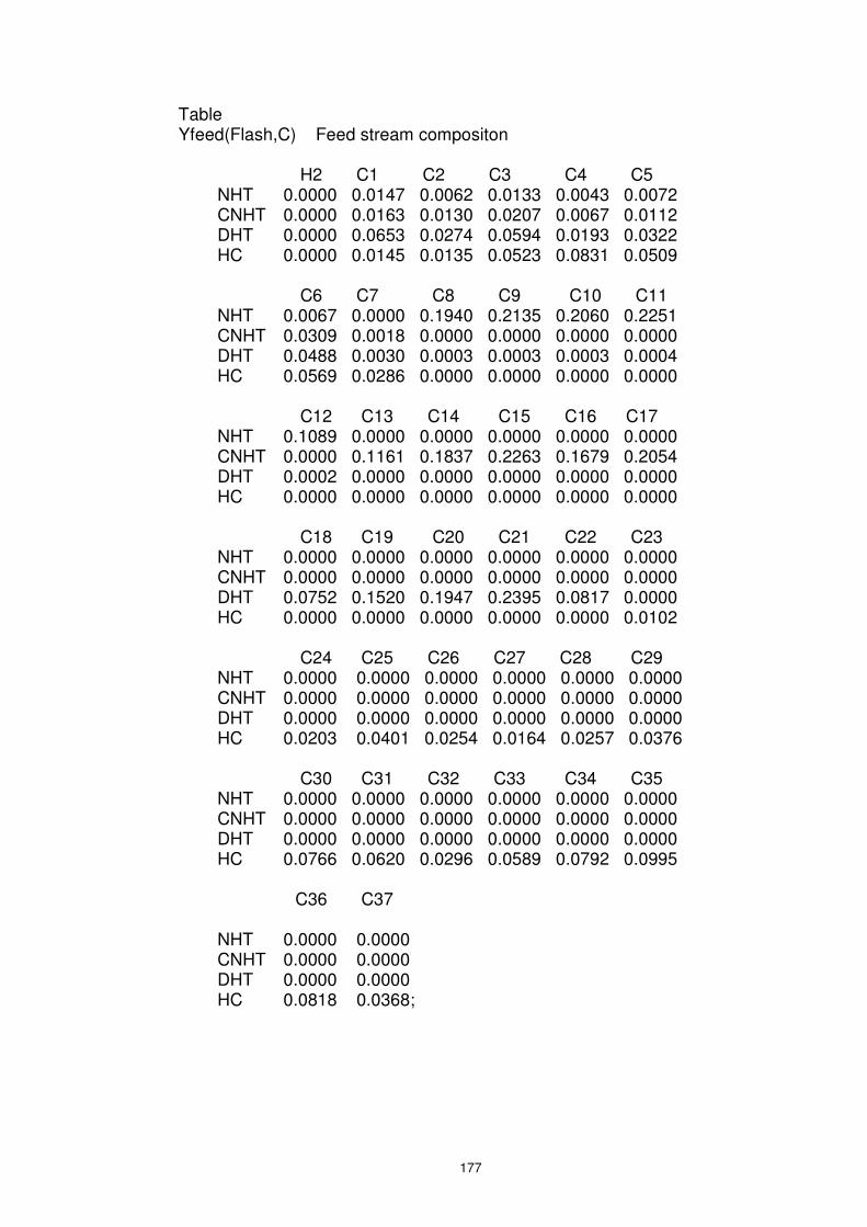
177
Table Yfeed(Flash,C) Feed stream compositon H2 C1 C2 C3 C4 C5 NHT 0.0000 0.0147 0.0062 0.0133 0.0043 0.0072 CNHT 0.0000 0.0163 0.0130 0.0207 0.0067 0.0112 DHT 0.0000 0.0653 0.0274 0.0594 0.0193 0.0322 HC 0.0000 0.0145 0.0135 0.0523 0.0831 0.0509 C6 C7 C8 C9 C10 C11 NHT 0.0067 0.0000 0.1940 0.2135 0.2060 0.2251 CNHT 0.0309 0.0018 0.0000 0.0000 0.0000 0.0000 DHT 0.0488 0.0030 0.0003 0.0003 0.0003 0.0004 HC 0.0569 0.0286 0.0000 0.0000 0.0000 0.0000 C12 C13 C14 C15 C16 C17 NHT 0.1089 0.0000 0.0000 0.0000 0.0000 0.0000 CNHT 0.0000 0.1161 0.1837 0.2263 0.1679 0.2054 DHT 0.0002 0.0000 0.0000 0.0000 0.0000 0.0000 HC 0.0000 0.0000 0.0000 0.0000 0.0000 0.0000 C18 C19 C20 C21 C22 C23 NHT 0.0000 0.0000 0.0000 0.0000 0.0000 0.0000 CNHT 0.0000 0.0000 0.0000 0.0000 0.0000 0.0000 DHT 0.0752 0.1520 0.1947 0.2395 0.0817 0.0000 HC 0.0000 0.0000 0.0000 0.0000 0.0000 0.0102 C24 C25 C26 C27 C28 C29 NHT 0.0000 0.0000 0.0000 0.0000 0.0000 0.0000 CNHT 0.0000 0.0000 0.0000 0.0000 0.0000 0.0000 DHT 0.0000 0.0000 0.0000 0.0000 0.0000 0.0000 HC 0.0203 0.0401 0.0254 0.0164 0.0257 0.0376 C30 C31 C32 C33 C34 C35 NHT 0.0000 0.0000 0.0000 0.0000 0.0000 0.0000 CNHT 0.0000 0.0000 0.0000 0.0000 0.0000 0.0000 DHT 0.0000 0.0000 0.0000 0.0000 0.0000 0.0000 HC 0.0766 0.0620 0.0296 0.0589 0.0792 0.0995 C36 C37 NHT 0.0000 0.0000 CNHT 0.0000 0.0000 DHT 0.0000 0.0000 HC 0.0818 0.0368;

178
Table KValue(Flash, C) K values foir the streams from the sources before flash calculation H2 C1 C2 C3 C4 C5 NHT 72.0140 11.2857 2.8654 0.9741 0.4130 0.3101 CNHT 42.6469 6.9179 1.8184 0.6346 0.2743 0.2058 DHT 49.5106 7.9403 2.0714 0.7185 0.3090 0.2320 HC 14.7690 3.0112 0.8698 0.3345 0.1560 0.1184 C6 C7 C8 C9 C10 C11 NHT 1.7641 7.4751 0.0332 0.0151 0.0073 0.0033 CNHT 1.0100 3.9462 0.0219 0.0102 0.0050 0.0023 DHT 1.1713 4.6353 0.0246 0.0114 0.0056 0.0025 HC 0.5004 2.0233 0.0147 0.0072 0.0014 0.0006 C12 C13 C14 C15 C16 C17 NHT 0.0015 0.0225 0.0085 0.0023 0.0007 0.0001 CNHT 0.0010 0.0184 0.0078 0.0026 0.0010 0.0002 DHT 0.0012 0.0145 0.0055 0.0015 0.0005 0.0001 HC 0.0002 0.0057 0.0022 0.0006 0.0002 0.0000 C18 C19 C20 C21 C22 C23 NHT 0.0000 0.0000 0.0000 0.0000 0.0000 0.1773 CNHT 0.0000 0.0000 0.0000 0.0000 0.0000 0.0967 DHT 0.0001 0.0000 0.0000 0.0000 0.0000 0.1357 HC 0.0000 0.0000 0.0000 0.0000 0.0000 0.0723 C24 C25 C26 C27 C28 C29 NHT 0.1029 0.0617 0.0356 0.0196 0.0231 0.0093 CNHT 0.0561 0.0337 0.0194 0.0107 0.0126 0.0051 DHT 0.0831 0.0528 0.0323 0.0190 0.0212 0.0095 HC 0.0460 0.0302 0.0191 0.0116 0.0128 0.0060 C30 C31 C32 C33 C34 C35 NHT 0.0035 0.0014 0.0005 0.0007 0.0001 0.0000 CNHT 0.0019 0.0008 0.0003 0.0004 0.0000 0.0000 DHT 0.0041 0.0019 0.0008 0.0010 0.0002 0.0000 HC 0.0027 0.0013 0.0006 0.0007 0.0001 0.0000 C36 C37 NHT 0.0000 0.0000 CNHT 0.0000 0.0000 DHT 0.0000 0.0000 HC 0.0000 0.0000;

179
Table Initial1(Flash, C) Purities of the components in the source streams before flash separation H2 C1 C2 C3 C4 C5 NHT 0.7587 0.1932 0.0120 0.0112 0.0017 0.0021 CNHT 0.6562 0.2788 0.0175 0.0122 0.0018 0.0022 DHT 0.7070 0.1500 0.0312 0.0356 0.0066 0.0076 HC 0.8122 0.0820 0.0091 0.0154 0.0120 0.0056 C6 C7 C8 C9 C10 C11 NHT 0.0092 5.e-11 0.0064 0.0032 0.0015 0.0007 CNHT 0.0241 0.0030 0.0001 0.0000 0.0000 0.0000 DHT 0.0429 0.0192 8.1E-6 4.2E-6 1.9E-6 9.8E-7 HC 0.0240 0.0355 0.0000 0.0000 0.0000 0.0000 C12 C13 C14 C15 C16 C17 NHT 0.0002 0.0000 0.0000 0.0000 0.0000 0.0000 CNHT 0.0000 0.0021 0.0014 0.0006 0.0002 4.1E-5 DHT 2.2E-7 0.0000 0.0000 0.0000 0.0000 0.0000 HC 0.0000 0.0000 0.0000 0.0000 0.0000 0.0000 C18 C19 C20 C21 C22 C23 NHT 0.0000 0.0000 0.0000 0.0000 0.0000 0.0000 CNHT 0.0000 0.0000 0.0000 0.0000 0.0000 0.0000 DHT 0.0000 0.0000 0.0000 0.0000 0.0000 0.0000 HC 0.0000 0.0000 0.0000 0.0000 0.0000 0.0007 C24 C25 C26 C27 C28 C29 NHT 0.0000 0.0000 0.0000 0.0000 0.0000 0.0000 CNHT 0.0000 0.0000 0.0000 0.0000 0.0000 0.0000 DHT 0.0000 0.0000 0.0000 0.0000 0.0000 0.0000 HC 0.0009 0.0012 0.0005 0.0002 0.0003 0.0002 C30 C31 C32 C33 C34 C35 NHT 0.0000 0.0000 0.0000 0.0000 0.0000 0.0000 CNHT 0.0000 0.0000 0.0000 0.0000 0.0000 0.0000 DHT 0.0000 0.0000 0.0000 0.0000 0.0000 0.0000 HC 0.0002 7.9E-5 1.6E-5 4.2E-5 1.0E-5 2.1E-6 C36 C37 NHT 0.0000 0.0000 CNHT 0.0000 0.0000 DHT 0.0000 0.0000 HC 2.5E-7 1.5E-08;

180
Table Initial2(Flash, C) Purities of the mix point H2 C1 C2 C3 C4 C5 NHT 0.7663 0.1937 0.0097 0.0091 0.0014 0.0018 CNHT 0.7049 0.2424 0.0140 0.0105 0.0015 0.0019 DHT 0.7542 0.1154 0.0223 0.0282 0.0092 0.0071 HC 0.9059 0.0458 0.0073 0.0095 0.0043 0.0027 C6 C7 C8 C9 C10 C11 NHT 0.0080 0.0002 0.0053 0.0027 0.0012 0.0006 CNHT 0.0180 0.0018 0.0010 0.0005 0.0002 0.0001 DHT 0.0366 0.0258 0.0000 0.0000 0.0000 0.0000 HC 0.0129 0.0105 0.0000 0.0000 0.0000 0.0000 C12 C13 C14 C15 C16 C17 NHT 0.0001 0.0000 0.0000 0.0000 0.0000 0.0000 CNHT 0.0000 0.0015 0.0010 0.0004 0.0001 0.0000 DHT 0.0000 0.0000 0.0000 0.0000 0.0000 0.0000 HC 0.0000 0.0000 0.0000 0.0000 0.0000 0.0000 C18 C19 C20 C21 C22 C23 NHT 0.0000 0.0000 0.0000 0.0000 0.0000 0.0000 CNHT 0.0000 0.0000 0.0000 0.0000 0.0000 0.0000 DHT 0.0000 0.0000 0.0000 0.0000 0.0000 0.0003 HC 0.0000 0.0000 0.0000 0.0000 0.0000 0.0002 C24 C25 C26 C27 C28 C29 NHT 0.0000 0.0000 0.0000 0.0000 0.0000 0.0000 CNHT 0.0000 0.0000 0.0000 0.0000 0.0000 0.0000 DHT 0.0003 0.0004 0.0001 0.0001 0.0001 0.0001 HC 0.0002 0.0003 0.0001 0.0000 0.0001 0.0001 C30 C31 C32 C33 C34 C35 NHT 0.0000 0.0000 0.0000 0.0000 0.0000 0.0000 CNHT 0.0000 0.0000 0.0000 0.0000 0.0000 0.0000 DHT 0.0001 0.0000 0.0000 0.0000 0.0000 0.0000 HC 0.0001 0.0000 0.0000 0.0000 0.0000 0.0000 C36 C37 NHT 0.0000 0.0000 CNHT 0.0000 0.0000 DHT 0.0000 0.0000 HC 0.0000 0.0000;

181
Table YreInitial(Flash, C) Purities of recycle H2 C1 C2 C3 C4 C5 NHT 0.7587 0.1934 0.0120 0.0111 0.0017 0.0021 CNHT 0.6549 0.2830 0.0157 0.0110 0.0017 0.0021 DHT 0.7144 0.1534 0.0343 0.0364 0.0058 0.0075 HC 0.8219 0.0666 0.0096 0.0157 0.0120 0.0056 C6 C7 C8 C9 C10 C11 NHT 0.0091 0.0000 0.0064 0.0032 0.0015 0.0007 CNHT 0.0241 0.0034 0.0000 0.0000 0.0000 0.0000 DHT 0.0428 0.0055 0.0000 0.0000 0.0000 0.0000 HC 0.0248 0.0395 0.0000 0.0000 0.0000 0.0000 C12 C13 C14 C15 C16 C17 NHT 0.0002 0.0000 0.0000 0.0000 0.0000 0.0000 CNHT 0.0000 0.0021 0.0014 0.0006 0.0002 0.0000 DHT 0.0000 0.0000 0.0000 0.0000 0.0000 0.0000 HC 0.0000 0.0000 0.0000 0.0000 0.0000 0.0000 C18 C19 C20 C21 C22 C23 NHT 0.0000 0.0000 0.0000 0.0000 0.0000 0.0000 CNHT 0.0000 0.0000 0.0000 0.0000 0.0000 0.0000 DHT 0.0000 0.0000 0.0000 0.0000 0.0000 0.0000 HC 0.0000 0.0000 0.0000 0.0000 0.0000 0.0007 C24 C25 C26 C27 C28 C29 NHT 0.0000 0.0000 0.0000 0.0000 0.0000 0.0000 CNHT 0.0000 0.0000 0.0000 0.0000 0.0000 0.0000 DHT 0.0001 0.0000 0.0000 0.0000 0.0000 0.0000 HC 0.0009 0.0012 0.0005 0.0002 0.0003 0.0002 C30 C31 C32 C33 C34 C35 NHT 0.0000 0.0000 0.0000 0.0000 0.0000 0.0000 CNHT 0.0000 0.0000 0.0000 0.0000 0.0000 0.0000 DHT 0.0000 0.0000 0.0000 0.0000 0.0000 0.0000 HC 0.0002 0.0001 0.0000 0.0000 0.0000 0.0000 C36 C37 NHT 0.0000 0.0000 CNHT 0.0000 0.0000 DHT 0.0000 0.0000 HC 0.0000 0.0000;

182
Table YH2Source(H2Sr,C) Purity of the sources from hydrogen producers H2 C1 C2 C3 C4 C5 H2Plant 0.9900 0.0100 0.0000 0.0000 0.0000 0.0000 CCR 0.8300 0.1700 0.0000 0.0000 0.0000 0.0000 C6 C7 C8 C9 C10 C11 H2Plant 0.0000 0.0000 0.0000 0.0000 0.0000 0.0000 CCR 0.0000 0.0000 0.0000 0.0000 0.0000 0.0000 C12 C13 C14 C15 C16 C17 H2Plant 0.0000 0.0000 0.0000 0.0000 0.0000 0.0000 CCR 0.0000 0.0000 0.0000 0.0000 0.0000 0.0000 C18 C19 C20 C21 C22 C23 H2Plant 0.0000 0.0000 0.0000 0.0000 0.0000 0.0000 CCR 0.0000 0.0000 0.0000 0.0000 0.0000 0.0000 C24 C25 C26 C27 C28 C29 H2Plant 0.0000 0.0000 0.0000 0.0000 0.0000 0.0000 CCR 0.0000 0.0000 0.0000 0.0000 0.0000 0.0000 C30 C31 C32 C33 C34 C35 H2Plant 0.0000 0.0000 0.0000 0.0000 0.0000 0.0000 CCR 0.0000 0.0000 0.0000 0.0000 0.0000 0.0000 C36 C37 NHT 0.0000 0.0000 CNHT 0.0000 0.0000; Parameter Ffeed(Flash) flowrate of Feed /NHT 32.79 CNHT 12.95 DHT 36.15 HC 37.62/

183
Variables z; Positive Variables Flowrate1(H2Sr,Flash) Flowrate2(Source,Flash) Fuel(Source) Slack1(Flash,C) Slack2(Flash,C) Slack3(Flash) Slack4(Flash) Slack5(Flash) Slack6(Flash) Slack7(Flash) Slack8(Flash) Slack9(Flash) Slack10(Flash) Slack11(Flash) Slack12(Flash) Slack13(Flash) Slack14(Flash) Fuel(Source) Purge to fuel Fpr(Flash) Flowrate of H2 between consumers Ypr(Flash,C) Compositions of H2 between consumers Fri(Flash) Flowrate of reactor inlet Yri(Flash,C) Compositions of reactor inlet Fre(Flash) Flowrate of recycle

184
Yre(Flash,C) Compositions of recycle Fmu(Flash) Flowrate of H2 makeup Ymu(Flash,C) Compositions of H2 makeup Fmix(Flash) Flowrate of mixture of recycle and makeup Ymix(Flash,C) Compositions of mixture of recycyel and makeup Ffi(Flash) Flowrate of flash inlet Yfi(Flash,C) Compositions of flash inlet Fliq(Flash) Flowrate of flash liquid Yliq(Flash,C) Compositions of flash liquid Fpu(Flash) Flowrate of Purge Yri.up(Flash,C)=0.9999; Yri.lo(Flash,C)=0; Yre.up(Flash,C)=0.9999; Yre.lo(Flash,C)=0; Ymu.up(Flash,C)=0.9999; Ymu.lo(Flash,C)=0; Ymix.up(Flash,C)=0.9999; Ymix.lo(Flash,C)=0; Yliq.up(Flash,C)=0.9999; Yliq.lo(Flash,C)=0; Fri.lo(Flash)=1e-3; Fre.lo(Flash)=1e-3; Fmu.lo(Flash)=1e-3; Fmix.lo(Flash)=1e-3; Fliq.lo(Flash)=1e-3; Fpu.lo(Flash)=1e-3; Ypr.up(Flash,C)=0.9999; Ypr.lo(Flash,C)=0; Ymix.up('NHT','H2')=0.8; Ymix.up('CNHT','H2')=0.8; Ymix.up('DHT','H2')=0.8; Ymix.up('HC','H2')=0.9; Ymix.lo('NHT','H2')=0.7; Ymix.lo('CNHT','H2')=0.6; Ymix.lo('DHT','H2')=0.7; Ymix.lo('HC','H2')=0.8;

185
Fmix.fx('NHT')= 53.93; Fmix.fx('CNHT')=49.67; Fmix.fx('DHT')=225.11; Fmix.fx('HC')=189.69; Fmix.up('NHT')= 60; Fmix.up('CNHT')=60; Fmix.up('DHT')=250; Fmix.up('HC')=220; Fmix.lo('NHT')= 45; Fmix.lo('CNHT')=40; Fmix.lo('DHT')=180; Fmix.lo('HC')=150; Fre.l('NHT')=47.28; Fre.l('CNHT')=42.04; Fre.l('DHT')=200.17; Fre.l('HC')=105.16; Equations equ1 Reactor inlet flowrate balance equ2 Reactor inlet composition balance equ3 Flash inlet flowrate balance equ4 Flash inlet composition balance *equ5 Flash calculation equ6 Flash inlet flowrate = outlet flowrate equ7 Flash outlet split composition balance equ8 Sum Yri to 1 equ9 Sum Yre to 1 equ10 Sum Ymu to 1 equ11 Sum Ymix to 1 equ12 Sum Yfi to 1 equ13 Sum Yliq to 1 *const1(Flash) equ14 mix point flowrate balance equ15 mix point composition balance equ16 Flash component balance equ17 H2Sr Flowrate balance equ18 H2Sr Component balance equ19 Define Fpr equ20 Define Ypr

186
equ21 Sum Ypr to 1 equ22 Fuel=Fpu-Fpr equ23 *equ24 *equ25 *equ26 obj objective function; *Flash calculation and network mass balance equ1(Flash).. Fri(Flash) =e= Fmix(Flash)+Ffeed(Flash)+Slack11(Flash)-Slack12(Flash); equ2(Flash,C).. Fri(Flash)*Yri(Flash,C) =e= Fmix(Flash)*Ymix(Flash,C)+Ffeed(Flash)*Yfeed(Flash,C)+Slack13(Flash,C)-Slack14(Flash,C); equ3(Flash).. Ffi(Flash) =e= Fri(Flash) - sum(C, R(Flash,C)); equ4(Flash,C).. Yfi(Flash,C)*Ffi(Flash) =e= Fri(Flash)*Yri(Flash,C)- R(Flash,C); *equ5(Flash,C).. Yfi(Flash,C) =e= Yre(Flash,C)*(1-f(Flash))+f(Flash)*Yliq(Flash,C)+Slack1(Flash,C); equ16(Flash,C).. Ffi(Flash)*Yfi(Flash,C) =e=Fre(Flash)*Yre(Flash,C)+Fpu(Flash)*Yre(Flash,C)+Fliq(Flash)*Yliq(Flash,C); equ6(Flash).. Fre(Flash)+Fpu(Flash)+Fliq(Flash) =e= Ffi(Flash); equ7(Flash,C).. Yre(Flash,C)=e= Yliq(Flash,C)*KValue(Flash,C)+Slack1(Flash,C)-Slack2(Flash,C); equ8(Flash).. sum(C,Yri(Flash,C))+Slack3(Flash)-Slack4(Flash) =e= 1; equ9(Flash).. sum(C,Yre(Flash,C)) =e= 1; equ10(Flash).. sum(C,Ymu(Flash,C)) +Slack7(Flash)-Slack8(Flash) =e= 1; equ11(Flash).. sum(C,Ymix(Flash,C)) +Slack9(Flash)-Slack10(Flash) =e= 1; equ12(Flash).. sum(C,Yfi(Flash,C))+Slack5(Flash)-Slack6(Flash) =e= 1;

187
equ13(Flash).. sum(C,Yliq(Flash,C)) =e= 1; equ14(Flash).. Fmix(Flash)=e= Fmu(Flash)+Fre(Flash)+Fpr(Flash); equ15(Flash,C).. Fmix(Flash)*Ymix(Flash,C)=e= Fmu(Flash)*Ymu(Flash,C)+Fre(Flash)*Yre(Flash,C)+Fpr(Flash)*Ypr(Flash,C); equ17(Flash).. Fmu(Flash)=e=sum(H2Sr,Flowrate1(H2Sr,Flash)); equ18(Flash,C).. Fmu(Flash)*Ymu(Flash,C)=e=sum(H2Sr,Flowrate1(H2Sr,Flash)*YH2Source(H2Sr,C)); equ19(Flash).. Fpr(Flash)=e= sum(Source$(ord(source) ne ord(flash)),Flowrate2(Source,Flash)); equ20(Flash,C).. Fpr(Flash)*Ypr(Flash,C)=e=sum(Source$(ord(source) ne ord(flash)),Flowrate2(Source,Flash)*Yre(Flash,C)); equ21(Flash).. sum(C,Ypr(Flash,C))=e=1; equ22.. sum(Flash,Flowrate1('CCR',Flash)) =e= 14.463; equ23.. sum(Flash,Flowrate1('H2plant',Flash)) =e= 103.7; obj.. z =e=sum((Flash),Flowrate1('H2Plant',Flash)) +sum((Flash,C),Slack1(Flash,C) +Slack2(Flash,C)+Slack13(Flash,C)+Slack14(Flash,C))*10000+sum(Flash,Slack3(Flash)+Slack4(Flash) +Slack5(Flash)+Slack6(Flash)+Slack7(Flash)+Slack8(Flash)+Slack9(Flash) +Slack10(Flash)+Slack11(Flash)+Slack12(Flash))*10000; option reslim = 1e20; option domlim = 10; option iterlim = 2e5; Model Basecase /all/ ; Basecase.workspace = 100;
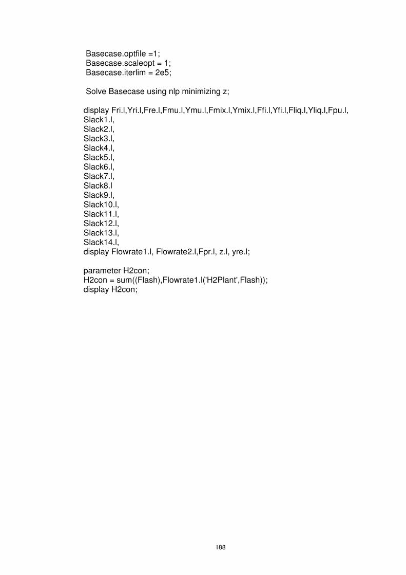
188
Basecase.optfile =1; Basecase.scaleopt = 1; Basecase.iterlim = 2e5; Solve Basecase using nlp minimizing z; display Fri.l,Yri.l,Fre.l,Fmu.l,Ymu.l,Fmix.l,Ymix.l,Ffi.l,Yfi.l,Fliq.l,Yliq.l,Fpu.l, Slack1.l, Slack2.l, Slack3.l, Slack4.l, Slack5.l, Slack6.l, Slack7.l, Slack8.l Slack9.l, Slack10.l, Slack11.l, Slack12.l, Slack13.l, Slack14.l, display Flowrate1.l, Flowrate2.l,Fpr.l, z.l, yre.l; parameter H2con; H2con = sum((Flash),Flowrate1.l('H2Plant',Flash)); display H2con;