reflection seismology - soest.hawaii.edu · reflection profile on the right.here we have assumed...

7

Reflection seismology

One of the most important applications of seismology involves the probing ofEarth’s internal structure by examining energy reflected at steep incidence anglesfrom subsurface layers. This technique may loosely be termed reflection seismologyand has been used extensively by the mining and petroleum industries to study theshallow crust, generally using portable instruments and artificial sources. However,similar methods can be applied to the deeper Earth using recordings of earthquakesor large explosions. Because reflected seismic waves are sensitive to sharp changesin velocity or density, reflection seismology can often provide much greater lateraland vertical resolution than can be obtained from study of direct seismic phasessuch as P and S (analyses of these arrivals may be termed refraction seismology).However, mapping of reflected phases into reflector depths requires knowledgeof the average background seismic velocity structure, to which typical reflectionseismic data are only weakly sensitive. Thus refraction experiments are a usefulcomplement to reflection experiments when independent constraints on the velocitystructure (e.g., from borehole logs) are unavailable.

Reflection seismic experiments are typically characterized by large numbers ofsources and receivers at closely spaced and regular intervals. Because the datavolume generally makes formal inversions too costly for routine processing, morepractical approximate methods have been widely developed to analyze the results.Simple time versus distance plots of the data can produce crude images of the subsur-face reflectors; these images become increasingly accurate as additional processingsteps are applied to the data.

Our discussion in this chapter will be limited to P-wave reflections, as the sourcesand receivers in most reflection seismic experiments are designed to produce andrecord P waves. Our focus will also mainly be concerned with the travel timerather than the amplitude of seismic reflections. Although amplitudes are some-times studied, historically amplitude information has assumed secondary impor-tance in reflection processing. Indeed often amplitudes are self-scaled prior to

181

182 7. R E F L E C T I O N S E I S M O L O G Y

plotting using automatic gain control (AGC) techniques. Finally, we will considera two-dimensional geometry, for which the sources, receivers, and reflectors areassumed to lie within a vertical plane. Recently, an increasing number of reflectionsurveys involve a grid of sources and receivers on the surface that are capable ofresolving three-dimensional Earth structure. Most of the concepts described in thischapter, such as common midpoint stacking and migration, are readily generalizedto three dimensions, although the data volume and computational requirements aremuch greater in this case.

Reflection seismology is a big topic, and only a brief outline can be presentedhere. For additional details, the reader is referred to texts such as Yilmaz (1987),Sheriff and Geldart (1995), and Claerbout (1976, 1985).

7.1 Zero-offset sections

Consider a collocated source and receiver at the surface above a horizontally layeredvelocity structure (Fig. 7.1). The downward propagating P waves from the sourceare reflected upward by each of the interfaces. The receiver will record a series ofpulses at times determined by the two-way P travel time between the surface andthe interfaces. If the velocity structure is known, these times can easily be convertedto depths.

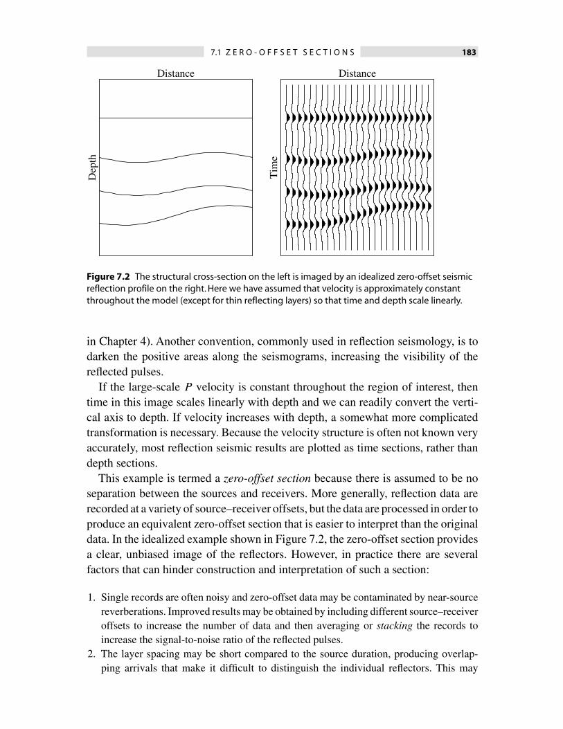
Now imagine repeating this as the source and receiver are moved to a seriesof closely spaced points along the surface. At each location, the receiver recordsthe reflected waves from the underlying structure. By plotting the results as afunction of time and distance, an image can be produced of the subsurface structure(Fig. 7.2). For convenience in interpreting the results, these record sections areplotted with downward increasing time (i.e., upside down compared with the plots

source & receiver

*

t

reflection seismogram

Figure 7.1 Seismic waves from a surface source are reflected by subsurface layers, producing aseismogram with discrete pulses for each layer. In this example, the velocity contrasts at theinterfaces are assumed to be small enough that multiple reflections can be ignored.

7.1 Z E R O - O F F S E T S E C T I O N S 183

Tim

e

Distance

Dep

th

Distance

Figure 7.2 The structural cross-section on the left is imaged by an idealized zero-offset seismicreflection profile on the right. Here we have assumed that velocity is approximately constantthroughout the model (except for thin reflecting layers) so that time and depth scale linearly.

in Chapter 4). Another convention, commonly used in reflection seismology, is todarken the positive areas along the seismograms, increasing the visibility of thereflected pulses.

If the large-scale P velocity is constant throughout the region of interest, thentime in this image scales linearly with depth and we can readily convert the verti-cal axis to depth. If velocity increases with depth, a somewhat more complicatedtransformation is necessary. Because the velocity structure is often not known veryaccurately, most reflection seismic results are plotted as time sections, rather thandepth sections.

This example is termed a zero-offset section because there is assumed to be noseparation between the sources and receivers. More generally, reflection data arerecorded at a variety of source–receiver offsets, but the data are processed in order toproduce an equivalent zero-offset section that is easier to interpret than the originaldata. In the idealized example shown in Figure 7.2, the zero-offset section providesa clear, unbiased image of the reflectors. However, in practice there are severalfactors that can hinder construction and interpretation of such a section:

1. Single records are often noisy and zero-offset data may be contaminated by near-sourcereverberations. Improved results may be obtained by including different source–receiveroffsets to increase the number of data and then averaging or stacking the records toincrease the signal-to-noise ratio of the reflected pulses.

2. The layer spacing may be short compared to the source duration, producing overlap-ping arrivals that make it difficult to distinguish the individual reflectors. This may


be addressed through a process termed deconvolution, which involves removing theproperties of the source from the records, providing a general sharpening of the image.

3. Lateral variations in structure or dipping layers may result in energy being scattered awayfrom purely vertical ray paths. These arrivals can bias estimates of reflector locationsand depths. By summing along possible sources of scattered energy, it is possible tocorrect the data for these effects; these techniques are termed migration and can resultin a large improvement in image quality.

4. Uncertainties in the overall velocity structure may prevent reliable conversion betweentime and depth and hinder application of stacking and migration techniques. Thus it iscritical to obtain the most accurate velocity information possible; in cases where outsideknowledge of the velocities are unavailable, the velocities must be estimated directlyfrom the reflection data.

We now discuss each of these topics in more detail.

7.2 Common midpoint stacking

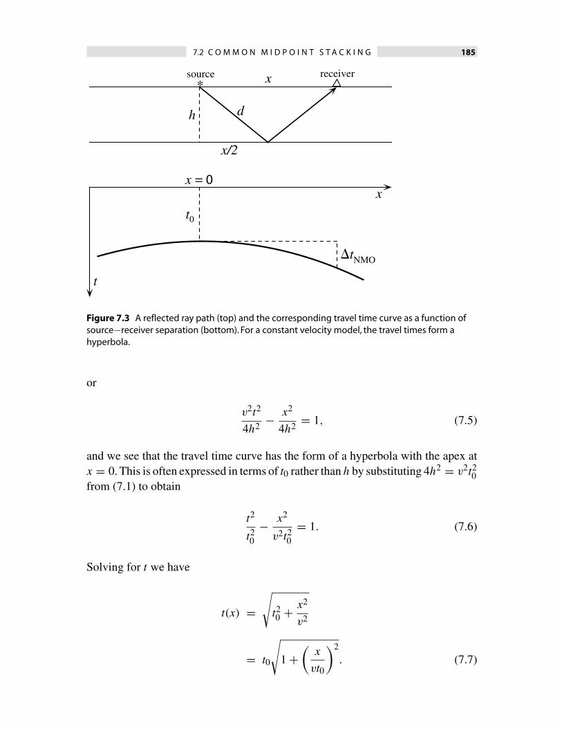
Consider a source recorded by a series of receivers at increasing distance. A pulsereflected from a horizontal layer will arrive earliest for the zero-offset receiver, whilethe arrivals at longer ranges will be delayed (Fig. 7.3). If the layer has thicknessh and a uniform P velocity of v, then the minimum travel time, t0, defined by thetwo-way vertical ray path, is

t0 = 2h

v. (7.1)

More generally, the travel time as a function of range, x, may be expressed as

t(x) = 2d

v, (7.2)

where d is the length of each leg of the ray path within the layer. From the geometry,we have

d2 = h2 + (x/2)2,

4d2 = 4h2 + x2.(7.3)

Squaring (7.2) and substituting for 4d2, we may write

v2t2 = x2 + 4h2 (7.4)

7.2 C O M M O N M I D P O I N T S T A C K I N G 185

source*

t

t0

x

h d

x/2

receiver

!tNMO

xx = 0

Figure 7.3 A reflected ray path (top) and the corresponding travel time curve as a function ofsource−receiver separation (bottom). For a constant velocity model, the travel times form ahyperbola.

or

v2t2

4h2 − x2

4h2 = 1, (7.5)

and we see that the travel time curve has the form of a hyperbola with the apex atx = 0. This is often expressed in terms of t0 rather than h by substituting 4h2 = v2t2

0from (7.1) to obtain

t2

t20

− x2

v2t20

= 1. (7.6)

Solving for t we have

t(x) =!

t20 + x2

v2

= t0

!

1 +"

x

vt0

#2

. (7.7)


For small offsets (x ≪ vt0) we may approximate the square root as

t(x) ≈ t0

$1 + 1

2(x/vt0)2%. (7.8)

The difference in time between the arrival at two different distances is termed themoveout and may be expressed as

!t = t(x2) − t(x1) = t0

&1 + (x2/vt0)2 − t0

&1 + (x1/vt0)2 (7.9)

≈ t0

$1 + 1

2(x2/vt0)2%

− t0

$1 + 1

2(x1/vt0)2%

≈ x22 − x2

1

2v2t0, (7.10)

where the approximate form is valid at small offsets. The normal moveout (NMO)is defined as the moveout from x = 0 and is given by

!tNMO = t0

&1 + (x/vt0)2 − t0 (7.11)

≈ x2

2v2t0. (7.12)

These equations are applicable for a single homogeneous layer. More complicatedexpressions can be developed for a series of layers overlying the target reflector orfor dipping layers (e.g., see Sheriff and Geldart, 1995).Alternatively, the ray tracingtheory developed in Chapter 4 can be applied to solve for the surface-to-reflectortravel time for any arbitrary velocity versus depth function v(z). Thus, a generalform for the NMO equation is

!tNMO(x) = 2[t(z, x/2) − t(z, 0)], (7.13)

where t(z, x) is the travel time from the surface to a point at depth z and horizontaloffset x.

A typical seismic reflection experiment deploys a large number of seismometersto record each source (these instruments are often called geophones in these appli-cations, or hydrophones in the case of pressure sensors for marine experiments).This is repeated for many different source locations. The total data set thus consistsof nm records, where n is the number of instruments and m is the number of sources.The arrival time of reflectors on each seismogram depends on the source–receiveroffset as well as the reflector depth. To display these results on a single plot, it isdesirable to combine the data in a way that removes the offset dependence in thetravel times so that any lateral variability in reflector depths can be seen clearly.

7.2 C O M M O N M I D P O I N T S T A C K I N G 187

sources* * * * *****

receivers

Figure 7.4 The source and receiver locations for a common midpoint (CMP) gather.

Figure 7.5 The left plot shows reflection seismograms at increasing source−receiver distance.The right plot shows the same profile after applying a NMO correction to each time series. Notethat this removes the range dependence in the arrival times.The NMO corrected records canthen be stacked to produce a single composite zero-offset record.

This is done by summing subsets of the data along the predicted NMO times toproduce a composite zero-offset profile. Data are generally grouped by predictedreflector location as illustrated in Figure 7.4.

Seismograms with common source–receiver midpoints are selected into what istermed a gather.ANMO correction is then applied to the records that shifts the timesto their zero-offset equivalent (as illustrated in Fig. 7.5). Notice that this correctionis not constant for each record but varies with time within the trace. This results inpulse broadening for the waveforms at longer offsets, but for short pulse lengthsand small offsets this effect is not large enough to cause problems. Finally the NMOcorrected data are summed and averaged to produce a single composite record that


represents the zero-offset profile at the midpoint location. This is called commonmidpoint (CMP) stacking, or sometimes common depth point (CDP) stacking. Thenumber of records, n, that are stacked is called the fold. For data with randomnoise, stacking can improve the signal-to-noise ratio of the records by a factor of√

n. CMP stacking can also minimize the influence of contaminating arrivals, suchas direct body waves or surface waves (Rayleigh waves, termed ground roll byreflection seismologists, are often the strongest arrival in reflection records), thatdo not travel along the predicted NMO travel time curves and thus do not stackcoherently.

CMP stacking has proven to be very successful in practice and is widely usedto produce reflection profiles at a minimum of computational expense. However, itrequires knowledge of the velocity-depth function to compute the NMO times andit does not explicitly account for the possibility of energy reflected or scattered fromnon-horizontal interfaces. We will discuss ways to address some of these limitationslater in this chapter, but first we examine source effects.

7.3 Sources and deconvolution

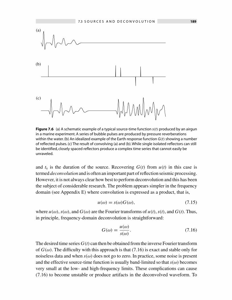
The ideal source for reflection seismology would produce a delta function or a veryshort impulsive wavelet that would permit closely spaced reflectors to be clearlyresolved. In practice, however, more extended sources must be used and the finitesource durations can cause complications in interpreting the data. For example, anairgun is often used for marine seismic reflection profiling. This device is towedbehind a ship and fires bursts of compressed air at regular intervals. This creates abubble that oscillates for several cycles before dissipating, producing a complicated“ringy’’ source-time function (e.g., Fig. 7.6). The reflection seismograms producedby such a source will reproduce this source-time function for each reflector. This isnot too confusing in the case where there are only a few, widely separated reflectors.However, if several closely spaced reflectors are present then it becomes difficultto separate the real structure from the source.

The combination of the Earth response with the source-time function is termedconvolution (see Appendix E) and may be written as

u(t) = s(t) ∗ G(t) ≡' ts

0s(τ)G(t − τ) dτ, (7.14)

where u(t) is the recorded seismogram, s(t) is the effective source-time function(i.e., what is actually recorded by the receiver; we assume that s(t) includes thereceiver response and any near-source attenuation), G(t) is the Earth response,

7.3 S O U R C E S A N D D E C O N V O L U T I O N 189

(a)

(b)

(c)

Figure 7.6 (a) A schematic example of a typical source-time function s(t) produced by an airgunin a marine experiment. A series of bubble pulses are produced by pressure reverberationswithin the water. (b) An idealized example of the Earth response function G(t) showing a numberof reflected pulses. (c) The result of convolving (a) and (b).While single isolated reflectors can stillbe identified, closely spaced reflectors produce a complex time series that cannot easily beunraveled.

and ts is the duration of the source. Recovering G(t) from u(t) in this case istermed deconvolution and is often an important part of reflection seismic processing.However, it is not always clear how best to perform deconvolution and this has beenthe subject of considerable research. The problem appears simpler in the frequencydomain (see Appendix E) where convolution is expressed as a product, that is,

u(ω) = s(ω)G(ω), (7.15)

where u(ω), s(ω), and G(ω) are the Fourier transforms of u(t), s(t), and G(t). Thus,in principle, frequency-domain deconvolution is straightforward:

G(ω) = u(ω)

s(ω). (7.16)

The desired time series G(t) can then be obtained from the inverse Fourier transformof G(ω). The difficulty with this approach is that (7.16) is exact and stable only fornoiseless data and when s(ω) does not go to zero. In practice, some noise is presentand the effective source-time function is usually band-limited so that s(ω) becomesvery small at the low- and high-frequency limits. These complications can cause(7.16) to become unstable or produce artifacts in the deconvolved waveform. To


address these difficulties, various methods for stabilizing deconvolution have beendeveloped. Often a time-domain approach is more efficient for data processing, inwhich case a filter is designed to perform the deconvolution directly on the data.

Although deconvolution is an important part of reflection data processing, nodeconvolution method is perfect, and some information is invariably lost in theprocess of convolution with the source-time function that cannot be recovered.For this reason, it is desirable at the outset to obtain as impulsive a source-timefunction as possible. Modern marine profiling experiments use airgun arrays thatare designed to minimize the amplitudes of the later bubble pulses, resulting inmuch cleaner and less ringy pulses than the example plotted in Figure 7.6a.

Another important source-time function is produced by a machine that vibratesover a range of frequencies. This is the most common type of source for shallowcrustal profiling on land and is termed vibroseis after the first commercial applica-tion of the method. The machine produces ground motion of the form of a modulatedsinusoid, termed a sweep,

v(t) = A(t) sin[2π(f0 + bt)t]. (7.17)

The amplitude A(t) is normally constant except for a taper to zero at the start and endof the sweep. The sweep lasts from about 5 to 40 s with frequencies ranging fromabout 10 to 60 Hz. The sweep duration is long enough compared with the intervalbetween seismic reflections that raw vibroseis records are difficult to interpret. Toobtain clearer records, the seismograms, u(t), are cross-correlated with the vibroseissweep function.

The cross-correlation f(t) between two real functions a(t) and b(t) is defined as

f(t) = a(t) ⋆ b(t) =' ∞

−∞a(τ − t)b(τ) dτ, (7.18)

where, following Bracewell (1978), we use the five-pointed star symbol ⋆ to denotecross-correlation; this should not be confused with the asterisk ∗ that indicates con-volution. The cross-correlation integral is very similar to the convolution integralbut without the time reversal of (7.14). Note that

a(t) ∗ b(t) = a(−t) ⋆ b(t) (7.19)

and that, unlike convolution, cross-correlation is not commutative:

a(t) ⋆ b(t) = b(t) ⋆ a(t). (7.20)

7.4 M I G R A T I O N 191

Cross-correlation of the vibroseis sweep function v(t) with the original seismogramu(t) yields the processed time series u′(t):

u′(t) = v(t) ⋆ u(t) =' ts

0v(τ − t)u(τ) dτ, (7.21)

where ts is the sweep duration. From (7.14) and replacing s(t) with v(t),we obtain

u′(t) = v(t) ⋆ [v(t) ∗ G(t)] (7.22)

= v(−t) ∗ [v(t) ∗ G(t)] (7.23)

= [v(−t) ∗ v(t)] ∗ G(t) (7.24)

= [v(t) ⋆ v(t)] ∗ G(t) (7.25)

= v′(t) ∗ G(t), (7.26)

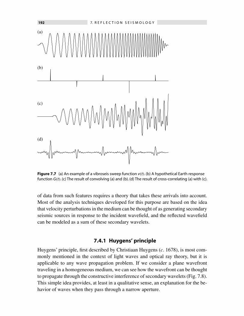
where we have used (7.19) and the associative rule for convolution. The cross-correlation of v(t) with itself, v′(t) = v(t) ⋆ v(t), is termed the autocorrelation ofv(t). This is a symmetric function, centered at t = 0, that is much more sharplypeaked than v(t). Thus, by cross-correlating the recorded seismogram with the vi-broseis sweep function v(t), one obtains a time series that represents the Earthresponse convolved with an effective source that is relatively compact. These re-lationships are illustrated in Figure 7.7. Cross-correlation with the source functionis a simple form of deconvolution that is sometimes termed spiking deconvolu-tion. Notice that the resulting time series is only an approximation to the desiredEarth response function G(t). More sophisticated methods of deconvolution canachieve better results, but G(t) can never be recovered perfectly since v(t) is band-limited and the highest and lowest frequency components of G(t) are lost in theconvolution.

7.4 Migration

Up to this point, we have modeled reflection seismograms as resulting from reflec-tions off horizontal interfaces. However, in many cases lateral variations in structureare present; indeed, resolving these features is often a primary goal of reflectionprofiling. Dipping, planar reflectors can be accommodated by modifying the NMOequations to adjust for differences between the updip and downdip directions. How-ever, more complicated structures will produce scattered and diffracted arrivals thatcannot be modeled by simple plane-wave reflections, and accurate interpretation


(a)

(b)

(c)

(d)

Figure 7.7 (a) An example of a vibroseis sweep function v(t). (b) A hypothetical Earth responsefunction G(t). (c) The result of convolving (a) and (b). (d) The result of cross-correlating (a) with (c).

of data from such features requires a theory that takes these arrivals into account.Most of the analysis techniques developed for this purpose are based on the ideathat velocity perturbations in the medium can be thought of as generating secondaryseismic sources in response to the incident wavefield, and the reflected wavefieldcan be modeled as a sum of these secondary wavelets.

7.4.1 Huygens’ principle

Huygens’ principle, first described by Christiaan Huygens (c. 1678), is most com-monly mentioned in the context of light waves and optical ray theory, but it isapplicable to any wave propagation problem. If we consider a plane wavefronttraveling in a homogeneous medium, we can see how the wavefront can be thoughtto propagate through the constructive interference of secondary wavelets (Fig. 7.8).This simple idea provides, at least in a qualitative sense, an explanation for the be-havior of waves when they pass through a narrow aperture.

7.4 M I G R A T I O N 193

(a)

(b)

t

t + !t

Figure 7.8 Illustrations ofHuygens’ principle. (a) A planewave at time t + !t can bemodeled as the coherent sumof the spherical wavefrontsemitted by point sources on thewavefront at time t. (b) A smallopening in a barrier to incidentwaves will produce a diffractedwavefront if the opening issmall compared to thewavelength.

The bending of the ray paths at the edges of the gap is termed diffraction. Thedegree to which the waves diffract into the “shadow’’ of the obstacle depends uponthe wavelength of the waves in relation to the size of the opening. At relatively longwavelengths (e.g., ocean waves striking a hole in a jetty), the transmitted waveswill spread out almost uniformly over 180◦. However, at short wavelengths thediffraction from the edges of the slot will produce a much smaller spreading in thewavefield. For light waves, very narrow slits are required to produce noticeablediffraction. These properties can be modeled using Huygens’ principle by comput-ing the effects of constructive and destructive interference at different wavelengths.

7.4.2 Diffraction hyperbolas

We can apply Huygens’ principle to reflection seismology by imagining that eachpoint on a reflector generates a secondary source in response to the incident wave-field. This is sometimes called the “exploding reflector’’ model. Consider a singlepoint scatterer in a zero-offset section (Fig. 7.9). The minimum travel time isgiven by

t0 = 2h

v, (7.27)


*

t

t0

x

x

h d

source & receiver

point scatterer

diffraction hyperbola Figure 7.9 A pointscatterer will produce acurved ‘‘reflector’’ in azero-offset section.

where h is the depth of the scatterer and v is the velocity (assumed constant inthis case). More generally, the travel time as a function of horizontal distance, x, isgiven by

t(x) = 2√

x2 + h2

v. (7.28)

Squaring and rearranging, this can be expressed as

v2t2

4h2 − x2

h2 = 1 (7.29)

or

t2

t20

− 4x2

v2t20

= 1 (7.30)

after substituting 4h2 = v2t20 from (7.27). The travel time curve for the scattered

arrival has the form of a hyperbola with the apex directly above the scattering point.Note that this hyperbola is steeper and results from a different ray geometry thanthe NMO hyperbola discussed in Section 7.2 (equation (7.5)). The NMO hyperboladescribes travel time for a reflection off a horizontal layer as a function of source–receiver distance; in contrast (7.30) describes travel time as a function of distance

7.4 M I G R A T I O N 195

Zero-offset sectionModel

Figure 7.10 The endpoint of a horizontal reflector will produce a diffracted arrival in azero-offset section.The reflector itself can be modeled as the coherent sum of the diffractionhyperbola from individual point scatterers.The diffracted phase, shown as the curved heavy line,occurs at the boundary of the region of scattered arrivals.

away from a point scatterer at depth for zero-offset data (the source and receiverare coincident).

7.4.3 Migration methods

Consider a horizontal reflector that is made up of a series of point scatterers, eachof which generates a diffraction hyperbola in a zero-offset profile (Fig. 7.10). Fol-lowing Huygens’ principle, these hyperbolas sum coherently only at the time ofthe main reflection; the later contributions cancel out. However, if the reflectorvanishes at some point, then there will be a diffracted arrival from the endpointthat will show up in the zero-offset data. This creates an artifact in the section thatmight be falsely interpreted as a dipping, curved reflector.

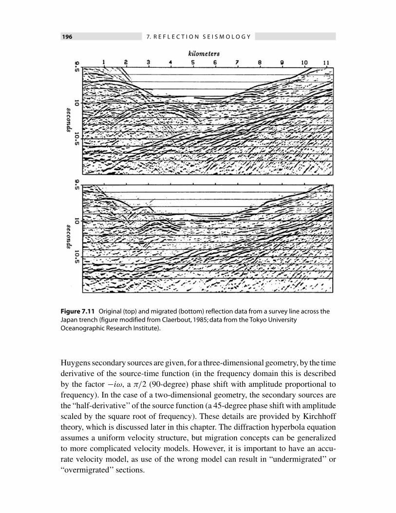
Techniques for removing these artifacts from reflection data are termed migrationand a number of different approaches have been developed. The simplest of thesemethods is termed diffraction summation migration and involves assuming thateach point in a zero-offset section is the apex of a hypothetical diffraction hyperbola.The value of the time series at that point is replaced by the average of the data fromadjacent traces taken at points along the hyperbola. In this way, diffraction artifactsare “collapsed’’ into their true locations in the migrated section. In many casesmigration can produce a dramatic improvement in image quality (e.g., Fig. 7.11).

Aproper implementation of diffraction summation migration requires wave prop-agation theory that goes beyond the simple ideas of Huygens’ principle. In partic-ular, the scattered amplitudes vary as a function of range and ray angle, and the


Figure 7.11 Original (top) and migrated (bottom) reflection data from a survey line across theJapan trench (figure modified from Claerbout, 1985; data from the Tokyo UniversityOceanographic Research Institute).

Huygens secondary sources are given, for a three-dimensional geometry, by the timederivative of the source-time function (in the frequency domain this is describedby the factor −iω, a π/2 (90-degree) phase shift with amplitude proportional tofrequency). In the case of a two-dimensional geometry, the secondary sources arethe “half-derivative’’of the source function (a 45-degree phase shift with amplitudescaled by the square root of frequency). These details are provided by Kirchhofftheory, which is discussed later in this chapter. The diffraction hyperbola equationassumes a uniform velocity structure, but migration concepts can be generalizedto more complicated velocity models. However, it is important to have an accu-rate velocity model, as use of the wrong model can result in “undermigrated’’ or“overmigrated’’ sections.

7.5 V E L O C I T Y A N A L Y S I S 197

In common practice, data from seismic reflection experiments are first processedinto zero-offset sections through CMP stacking. The zero-offset section is thenmigrated to produce the final result. This is termed poststack migration. BecauseCMP stacking assumes horizontal layering and may blur some of the details of theoriginal data, better results can be obtained if the migration is performed prior tostacking. This is called prestack migration. Although prestack migration is knownto produce superior results, it is not implemented routinely owing to its much greatercomputational cost.

7.5 Velocity analysis

Knowledge of the large-scale background seismic velocity structure is essential forreflection seismic processing (for both stacking and migration) and for translatingobserved events from time to depth. Often this information is best obtained fromresults derived independently of the reflection experiment, such as from boreholelogs or from a collocated refraction experiment. However, if such constraints are notavailable a velocity profile must be estimated from the reflection data themselves.This can be done in several different ways.

One approach is to examine the travel time behavior of reflectors in CMP gathers.From (7.7), we have for a reflector overlain by material of uniform velocity v:

t2(x) = t20 + x2

v2 (7.31)

= t20 + u2x2, (7.32)

where u = 1/v is the slowness of the layer. From observations of the NMO offsetsin a CMP gather, one can plot values of t2 versus x2. Fitting a straight line to thesepoints then gives the intercept t2

0 and the slope u2 = 1/v2. Velocity often is notconstant with depth, but this equation will still yield a velocity, which can be shownto be approximately the root-mean-square (rms) velocity of the overlying medium,that is, for n layers

v2 ≈(n

i=1 v2i!ti(n

i=1!ti, (7.33)

where !ti is the travel time through the ith layer.Another method is to plot NMO corrected data as a function of offset for different

velocity models to see which model best removes the range dependence in the dataor produces the most coherent image following CMP stacking. As in the case of the


t2(x2) plotting method, this will only resolve the velocities accurately if a reasonablespread in source–receiver offsets are available. Zero-offset data have no directvelocity resolution; the constraints on velocity come from the NMO offsets in thetravel times with range. Thus, wider source–receiver profiling generally producesbetter velocity resolution, with the best results obtained in the case where receiverranges are extended far enough to capture the direct refracted phases. However,even zero-offset data can yield velocity information if diffraction hyperbolas arepresent in the zero-offset profiles, as the curvature of these diffracted phases canbe used to constrain the velocities. One approach is to migrate the section withdifferent migration velocities in order to identify the model that best removes theartifacts in the profile.

7.5.1 Statics corrections

Often strong near-surface velocity heterogeneity produces time shifts in the recordsthat can vary unpredictably between sources and stations. This could be causedby topography/bathymetry or a sediment layer of variable thickness. The result-ing “jitter’’ in the observed reflected pulses (Fig. 7.12) can hinder applicationof stacking and migration techniques and complicate interpretation of the results.Thus, it is desirable to remove these time shifts prior to most processing of theresults. This is done by applying timing corrections, termed statics corrections, tothe data. In the case of the receivers, these are analogous to the station terms (the

Figure 7.12 Small time shifts on individual records produce offsets in reflectors in CMP gathers(left plot) that prevent coherent stacking of these phases in data processing.These shifts can beremoved by applying static corrections (right plot).

7.6 R E C E I V E R F U N C T I O N S 199

average travel time residual at a particular station for many different events) usedin travel time inversions for Earth structure. Statics may be computed by trackingthe arrival time of a reference phase, such as a refracted arrival. Often automaticmethods are applied to find the time shifts that best smooth the observed reflectors.The goal is to shift the timing of the individual records such that reflectors will stackcoherently. This problem is tractable since the time shifts are generally fairly small,and solutions for the time shifts are overdetermined in typical reflection experiments(multiple receivers for each source, multiple sources for each receiver).

7.6 Receiver functions

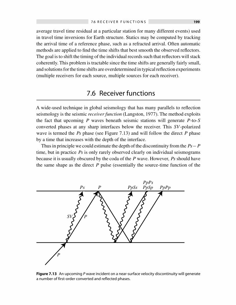
A wide-used technique in global seismology that has many parallels to reflectionseismology is the seismic receiver function (Langston, 1977). The method exploitsthe fact that upcoming P waves beneath seismic stations will generate P-to-Sconverted phases at any sharp interfaces below the receiver. This SV -polarizedwave is termed the Ps phase (see Figure 7.13) and will follow the direct P phaseby a time that increases with the depth of the interface.

Thus in principle we could estimate the depth of the discontinuity from the Ps−P

time, but in practice Ps is only rarely observed clearly on individual seismogramsbecause it is usually obscured by the coda of the P wave. However, Ps should havethe same shape as the direct P pulse (essentially the source-time function of the

P

SV

PPs PpSsPpPs

PpPpPpSp

P

Figure 7.13 An upcoming P wave incident on a near-surface velocity discontinuity will generatea number of first-order converted and reflected phases.


earthquake as modified by attenuation along the ray path), and thus, just as in thevibroseis example discussed above, Ps can often be revealed by deconvolving the P

pulse from the rest of the seismogram. The deconvolved waveform is termed thereceiver function. For the steeply incident ray paths of distant teleseisms, P appearsmost strongly on the vertical component and Ps on the radial component. Thus, thesimplest approach extracts the direct P pulse from the vertical channel and performsthe deconvolution on the radial component. However, somewhat cleaner results canbe obtained by applying a transformation to estimate the upcoming P and SV wavefield from the observed vertical and radial components. This transformation mustinclude the effect of the free-surface reflected phases (i.e., the downgoing P andSV pulses) on the observed displacement at the surface.

Following Kennett (1991) and Bostock (1998), we may express the upcomingP and SV components at the surface as

)P

SV

*=)

pβ2/α (1 − 2β2p2)/2αηα(1 − 2β2p2)/2βηβ −pβ

* )UR

UZ

*, (7.34)

where UR and UZ are the radial and vertical components, p is the ray parameter, αand β are the P and S velocities at the surface, and the P and S vertical slownessesare given by ηα =

+α−2 − p2 and ηβ =

+β−2 − p2. Note that here we adopt the

sign convention, opposite to that in Bostock (1998), that the incident P wave hasthe same polarity on the vertical and radial seismometer components.

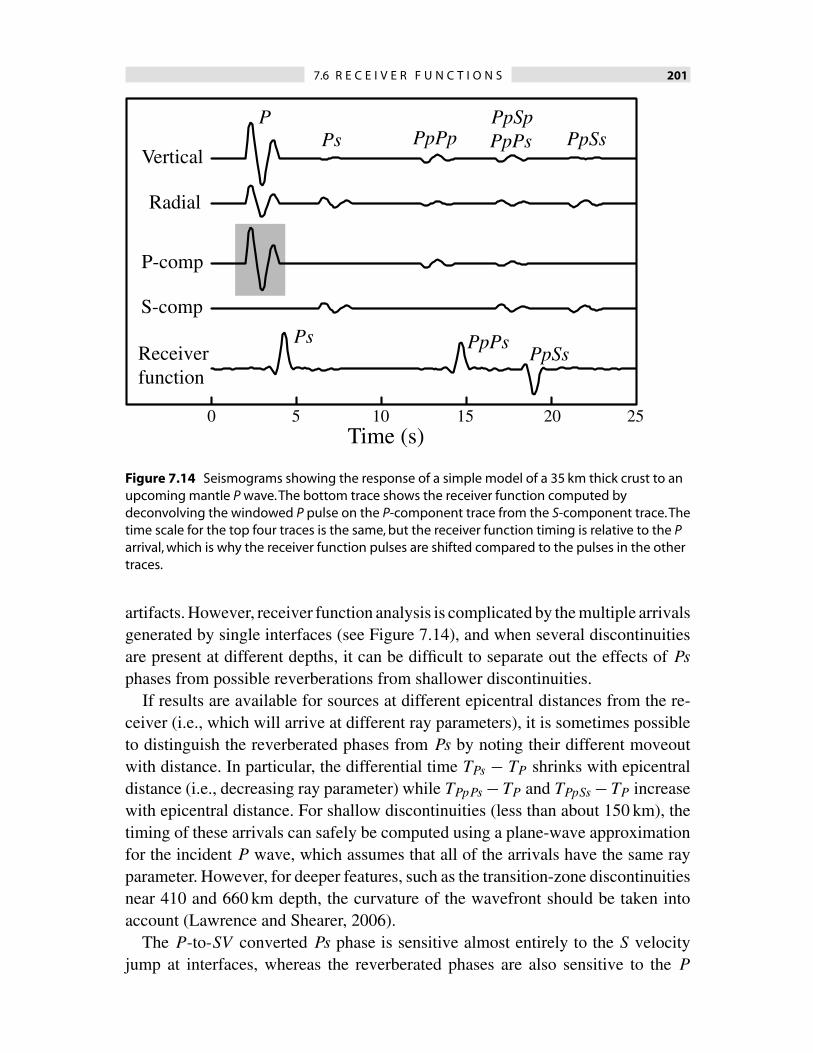
This transformation has been applied to the vertical and radial channels in Figure7.14 and shows how the resulting P and SV components isolate the different phases.In particular, note that the direct P arrival appears only on the P component, whilePs appears only on the SV component. The reverberated phases are seen separatelyon the P and S components according to whether the upcoming final leg beneaththe receiver is P or SV . The resulting receiver function is plotted at the bottom ofFigure 7.14, and in this case has pulses at times given by the differential times of Ps,PpPs and PpSs with respect to the direct P arrival. In general, the receiver-functionpulse shapes are more impulsive and symmetric than that of the P waveform, buttheir exact shape will depend on the deconvolution method and the bandwidth ofthe data.

Analysis of receiver functions is similar to reflection seismology in many re-spects. Both methods study seismic phases resulting from velocity jumps at inter-faces beneath receivers and require knowledge of the background seismic velocitiesto translate the timing of these phases into depth. Both often use deconvolution andstacking to improve the signal-to-noise ratio of the results. When closely spacedseismic receivers are available (for example, a seismometer array), migration meth-ods can be used to image lateral variations in structure and correct for scattering

7.6 R E C E I V E R F U N C T I O N S 201

0 5 10 15 20 25Time (s)

PPs PpSsPpPsPpPp

PpSp

Ps PpPsPpSs

Vertical

Radial

P-comp

S-comp

Receiverfunction

Figure 7.14 Seismograms showing the response of a simple model of a 35 km thick crust to anupcoming mantle P wave.The bottom trace shows the receiver function computed bydeconvolving the windowed P pulse on the P-component trace from the S-component trace.Thetime scale for the top four traces is the same, but the receiver function timing is relative to the Parrival, which is why the receiver function pulses are shifted compared to the pulses in the othertraces.

artifacts. However, receiver function analysis is complicated by the multiple arrivalsgenerated by single interfaces (see Figure 7.14), and when several discontinuitiesare present at different depths, it can be difficult to separate out the effects of Ps

phases from possible reverberations from shallower discontinuities.If results are available for sources at different epicentral distances from the re-

ceiver (i.e., which will arrive at different ray parameters), it is sometimes possibleto distinguish the reverberated phases from Ps by noting their different moveoutwith distance. In particular, the differential time TPs − TP shrinks with epicentraldistance (i.e., decreasing ray parameter) while TPpPs −TP and TPpSs −TP increasewith epicentral distance. For shallow discontinuities (less than about 150 km), thetiming of these arrivals can safely be computed using a plane-wave approximationfor the incident P wave, which assumes that all of the arrivals have the same rayparameter. However, for deeper features, such as the transition-zone discontinuitiesnear 410 and 660 km depth, the curvature of the wavefront should be taken intoaccount (Lawrence and Shearer, 2006).

The P-to-SV converted Ps phase is sensitive almost entirely to the S velocityjump at interfaces, whereas the reverberated phases are also sensitive to the P


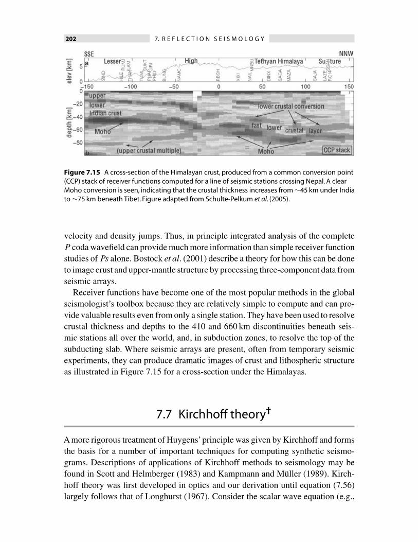
Figure 7.15 A cross-section of the Himalayan crust, produced from a common conversion point(CCP) stack of receiver functions computed for a line of seismic stations crossing Nepal. A clearMoho conversion is seen, indicating that the crustal thickness increases from ∼45 km under Indiato ∼75 km beneath Tibet. Figure adapted from Schulte-Pelkum et al. (2005).

velocity and density jumps. Thus, in principle integrated analysis of the completeP coda wavefield can provide much more information than simple receiver functionstudies of Ps alone. Bostock et al. (2001) describe a theory for how this can be doneto image crust and upper-mantle structure by processing three-component data fromseismic arrays.

Receiver functions have become one of the most popular methods in the globalseismologist’s toolbox because they are relatively simple to compute and can pro-vide valuable results even from only a single station. They have been used to resolvecrustal thickness and depths to the 410 and 660 km discontinuities beneath seis-mic stations all over the world, and, in subduction zones, to resolve the top of thesubducting slab. Where seismic arrays are present, often from temporary seismicexperiments, they can produce dramatic images of crust and lithospheric structureas illustrated in Figure 7.15 for a cross-section under the Himalayas.

7.7 Kirchhoff theory†

A more rigorous treatment of Huygens’principle was given by Kirchhoff and formsthe basis for a number of important techniques for computing synthetic seismo-grams. Descriptions of applications of Kirchhoff methods to seismology may befound in Scott and Helmberger (1983) and Kampmann and Muller (1989). Kirch-hoff theory was first developed in optics and our derivation until equation (7.56)largely follows that of Longhurst (1967). Consider the scalar wave equation (e.g.,

7.7 K I R C H H O F F T H E O R Y 203

equation (3.31) where φ is the P-wave potential)

∇2φ = 1c2

∂2φ

∂t2 , (7.35)

where c is the wave velocity. Now assume a harmonic form for φ, that is, at aparticular frequency ω we have the monochromatic function

φ = ψ(r)e−iωt = ψ(r)e−ikct, (7.36)

where r is the position and k = ω/c is the wavenumber. Note that we have separatedthe spatial and temporal parts of φ. We then have

∇2φ = e−ikct∇2ψ (7.37)

and

∂2φ

∂t2 = −k2c2ψe−ikct (7.38)

and (7.35) becomes

∇2ψ = −k2ψ. (7.39)

This is a time-independent wave equation for the space-dependent part of φ. It isalso sometimes termed the Helmholtz equation.

Next, recall Green’s theorem from vector calculus. If ψ1 and ψ2 are two contin-uous single-valued functions with continuous derivatives, then for a closed surfaceS

'

V(ψ2∇2ψ1 − ψ1∇2ψ2) dv =

'

S

"ψ2∂ψ1

∂n− ψ1

∂ψ2

∂n

#dS, (7.40)

where the volume integral is over the volume enclosed by S, and ∂/∂n is the deriva-tive with respect to the outward normal vector to the surface. Now assume that bothψ1 and ψ2 satisfy (7.39), that is,

∇2ψ1 = −k2ψ1, (7.41)

∇2ψ2 = −k2ψ2. (7.42)

In this case, the left part of (7.40) vanishes and the surface integral must be zero:'

S

"ψ2∂ψ1

∂n− ψ1

∂ψ2

∂n

#dS = 0. (7.43)

Now suppose that we are interested in evaluating the disturbance at the point P ,which is enclosed by the surface S (Fig. 7.16). We set ψ1 = ψ, the amplitude of


Figure 7.16 A point P surrounded by asurface S of arbitrary shape. Kirchhoff’sformula is derived by applying Green’stheorem to the volume between S and aninfinitesimal sphere " surrounding P.

the harmonic disturbance. We are free to choose any function for ψ2, provided italso satisfies (7.39). It will prove useful to define ψ2 as

ψ2 = eikr

r, (7.44)

where r is the distance from P . This function has a singularity at r = 0 and sothe point P must be excluded from the volume integral for Green’s theorem to bevalid. We can do this by placing a small sphere , around P . Green’s theorem maynow be applied to the volume between , and S; these surfaces, together, make upthe integration surface. On the surface of the small sphere the outward normal tothis volume is opposite to the direction of r and thus ∂/∂n can be replaced with−∂/∂r and the surface integral over , may be expressed as

'

,

"ψ2∂ψ

∂n− ψ

∂ψ2

∂n

#dS =

'

,

,−eikr

r

∂ψ

∂r+ ψ

∂

∂r

-eikr

r

./

dS

='

,

,−eikr

r

∂ψ

∂r+ ψ

-−eikr

r2 + ikeikr

r

./

dS.

(7.45)

Now let us change this to an integral over solid angle- from the point P , in whichdS on , subtends d- and dS = r2 d-. Then

'

,='

around P

"−reikr ∂ψ

∂r− ψeikr + rikψeikr

#d-. (7.46)

Now consider the limit as r goes to zero. Assuming that ψ does not vanish, thenonly the second term in this expression survives. Thus as r → 0

'

,→'

−ψeikrd-. (7.47)


As the surface, collapses around P , the value ofψ on the surface may be assumedto be constant and equal to ψP , its value at P . Thus

'

,→

'−ψPeikrd- (7.48)

= −ψP

'eikrd- (7.49)

= −ψP

'd- since eikr → 1 as r → 0 (7.50)

= −4πψP . (7.51)

From (7.43) we know that0S+, = 0, so we must have

0S = +4πψP , or

4πψP ='

S

,eikr

r

∂ψ

∂n− ψ

∂

∂n

-eikr

r

./

dS (7.52)

='

S

,eikr

r

∂ψ

∂n− ψeikr ∂

∂n

"1r

#− ikψeikr

r

∂r

∂n

/

dS, (7.53)

since ∂∂n = ∂

∂r∂r∂n . This is often called Helmholtz’s equation. Since φ = ψe−ikct

(7.35), we have

ψ = φeikct (7.54)

and (7.53) becomes

φP = 14π

e−ikct

'

S

,eikr

r

∂ψ

∂n− ψeikr ∂

∂n

"1r

#− ikψeikr

r

∂r

∂n

/

dS

= 14π

'

S

,e−ik(ct−r)

r

∂ψ

∂n− ψe−ik(ct−r) ∂

∂n

"1r

#− ikψe−ik(ct−r)

r

∂r

∂n

/

dS.

(7.55)

This expression gives φ(t) at the point P . Note that the term ψe−ik(ct−r) =ψe−ikc(t−r/c) is the value of φ at the element dS at the time t − r/c. This timeis referred to as the retarded value of φ and is written [φ]t−r/c. In this way, we canexpress (7.55) as

φP = 14π

'

S

-1r

)∂φ

∂n

*

t−r/c

− ∂

∂n

"1r

#[φ]t−r/c + 1

cr

∂r

∂n

)∂φ

∂t

*

t−r/c

.

dS,

(7.56)


Figure 7.17 The raygeometry for a single pointon a surface dS separating asource and receiver.

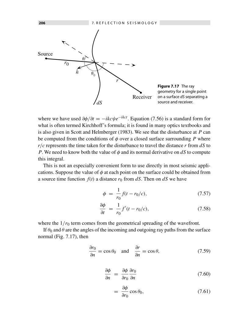
where we have used ∂φ/∂t = −ikcψe−ikct . Equation (7.56) is a standard form forwhat is often termed Kirchhoff’s formula; it is found in many optics textbooks andis also given in Scott and Helmberger (1983). We see that the disturbance at P canbe computed from the conditions of φ over a closed surface surrounding P wherer/c represents the time taken for the disturbance to travel the distance r from dS toP . We need to know both the value of φ and its normal derivative on dS to computethis integral.

This is not an especially convenient form to use directly in most seismic appli-cations. Suppose the value of φ at each point on the surface could be obtained froma source time function f(t) a distance r0 from dS. Then on dS we have

φ = 1r0

f(t − r0/c), (7.57)

∂φ

∂t= 1

r0f ′(t − r0/c), (7.58)

where the 1/r0 term comes from the geometrical spreading of the wavefront.If θ0 and θ are the angles of the incoming and outgoing ray paths from the surface

normal (Fig. 7.17), then

∂r0

∂n= cos θ0 and

∂r

∂n= cos θ, (7.59)

∂φ

∂n= ∂φ

∂r0

∂r0

∂n(7.60)

= ∂φ

∂r0cos θ0, (7.61)


and

∂

∂n

"1r

#= ∂r

∂n

∂

∂r

"1r

#(7.62)

= − 1r2 cos θ. (7.63)

We can evaluate ∂φ/∂r0 using the chain rule:

∂

∂r0

"1r0

f(t − r0/c)

#= − 1

r20

f(t − r0/c) − 1cr0

f ′(t − r0/c) (7.64)

since ∂∂r0

= ∂t∂r0

∂∂t = −1

c∂∂t . Putting (7.57)–(7.64) into (7.56), we have

φP(t) = 14π

'

S

-−1

rr20

cos θ0 + 1r2r0

cos θ

.

f(t − r/c − r0/c) dS

+ 14π

'

S

" −1crr0

cos θ0 + 1crr0

cos θ#

f ′(t − r/c − r0/c) dS. (7.65)

The negative signs arise from our definition of n in the direction opposing r0; theseterms are positive since cos θ0 is negative. Equation (7.65) may also be expressedin terms of convolutions with f(t) and f ′(t):

φP(t) = 14π

'

Sδ

"t − r + r0

c

#-−1

rr20

cos θ0 + 1r2r0

cos θ

.

dS ∗ f(t)

+ 14π

'

Sδ

"t − r + r0

c

#" −1crr0

cos θ0 + 1crr0

cos θ#

dS ∗ f ′(t).

(7.66)

Notice that the f(t) terms contain an extra factor of 1/r or 1/r0. For this reasonthey are most important close to the surface of integration and can be thought of asnear-field terms. In practice, the source and receiver are usually sufficiently distantfrom the surface (i.e., λ ≪ r, r0) that φP is well approximated by using only thefar-field f ′(t) terms. In this case we have

φP(t) = 14πc

'

Sδ

"t − r + r0

c

#1

rr0(− cos θ0 + cos θ) dS ∗ f ′(t). (7.67)

This formula is the basis for many computer programs that compute Kirchhoffsynthetic seismograms.


Figure 7.18 Kirchhoff theory can be used to compute the effect of an irregular boundary onboth transmitted and reflected waves.

7.7.1 Kirchhoff applications

Probably the most common seismic application of Kirchhoff theory involves thecase of an irregular interface between simpler structure on either side. Kirchhofftheory can be used to provide an approximate solution for either the transmitted orreflected wavefield due to this interface (Fig. 7.18). For example, we might want tomodel the effect of irregularities on the core–mantle boundary, the Moho, the seafloor, or a sediment–bedrock interface. In each case, there is a significant velocitycontrast across the boundary.

Let us consider the reflected wave generated by a source above an undulatinginterface. Assume that the incident wavefield is known and can be described withgeometrical ray theory. Then we make the approximation that the reflected wave-field just above the interface is given by the plane-wave reflection coefficient forthe ray incident on the surface. This approximation is sometimes called the Kirch-hoff, physical optics, or tangent plane hypothesis (Scott and Helmberger, 1983).Each point on the surface reflects the incident pulse as if there were an infiniteplane tangent to the surface at that point. Considering only the far-field terms, wethen have

φP(t) = 14πc

'

Sδ

"t − r + r0

c

#R(θ0)

rr0(cos θ0 + cos θ) dS ∗ f ′(t), (7.68)

where R(θ0) is the reflection coefficient, θ0 is the angle between the incident rayand the surface normal, and θ is the angle between the scattered ray and the surfacenormal (see Fig. 7.19).

If the overlying layer is not homogeneous, then the 1/r and 1/r0 terms must bereplaced with the appropriate source-to-interface and interface-to-receiver geomet-rical spreading coefficients. In some cases, particularly for obliquely arriving rays,


nr0 r

Source Receiver

Figure 7.19 Ray angles relative to the surface normal for a reflected wave geometry.

Source Receiver

cornerdiffractedwave

reflectedwave

Figure 7.20 This structure will produce both a direct reflected pulse and a diffracted pulse forthe source−receiver geometry shown.

the reflection coefficient R may become complex. If this occurs, then this equationwill have both a real and an imaginary part. The final time series is obtained byadding the real part to the Hilbert transform of the imaginary part.

The Kirchhoff solution will correctly model much of the frequency dependenceand diffracted arrivals in the reflected wavefield. These effects are not obtainedthrough geometrical ray theory alone, even if 3-D ray tracing is used. For example,consider a source and receiver above a horizontal interface containing a verti-cal fault (Fig. 7.20). Geometrical ray theory will produce only the main reflectedpulse from the interface, while Kirchhoff theory will provide both the main pulseand the secondary pulse diffracted from the corner. However, Kirchhoff theoryalso has its limitations, in that it does not include any multiple scattering ordiffractions along the interface; these might be important in more complicatedexamples.


7.7.2 How to write a Kirchhoff program

As an illustration, let us list the steps involved in writing a hypothetical Kirchhoffcomputer program to compute the reflected wavefield from a horizontal interfacewith some irregularities.

1. Specify the source and receiver locations.2. Specify the source-time function f(t).3. Compute f ′(t), the derivative of the source-time function.4. Initialize to zero a time series J(t), with sample interval dt, that will contain the output

of the Kirchhoff integral.5. Specify the interface with a grid of evenly spaced points in x and y. At each grid point,

we must know the height of the boundary z and the normal vector to the surface n. Wealso require the surface area, dA, corresponding to the grid point. This is approximatelydx dy where dx and dy are the grid spacings in the x and y directions, respectively (if asignificant slope is present at the grid point, the actual surface area is greater and thiscorrection must be taken into account). The grid spacing should be finer than the scalelength of the irregularities.

6. At each grid point, trace rays to the source and receiver. Determine the travel times tothe source and receiver, the ray angles to the local normal vector (θ0 and θ), and thegeometrical spreading factors g0 (source-to-surface) and g (surface-to-receiver).

7. At each grid point, compute the reflection coefficient R(θ0) and the factor cos θ0 +cos θ.8. At each grid point, compute the product R(θ0)(cos θ0 + cos θ)dA/(4πcg0g). Add the

result to the digitized point of J(t) that is closest to the total source-surface-receivertravel time, after first dividing the product by the digitization interval dt.

9. Repeat this for all grid points that produce travel times within the time interval ofinterest.

10. Convolve J(t) with f ′(t), the derivative of the source-time function, to produce the finalsynthetic seismogram.

11. (very important) Repeat this procedure at a finer grid spacing, dx and dy, to verify thatthe same result is obtained. If not, the interface is undersampled and a finer grid mustbe used.

Generally the J(t) function will contain high-frequency numerical “noise’’ that isremoved through the convolution with f ′(t). It is computationally more efficientto compute f ′(t) and convolve with J(t) than to compute J ′(t) and convolve withf(t), particularly when multiple receiver positions are to be modeled.

7.7.3 Kirchhoff migration

Kirchhoff results can be used to implement migration methods for reflection seismicdata that are consistent with wave propagation theory. For zero-offset data, θ0 = θ

7.8 E X E R C I S E S 211

and r0 = r and (7.68) becomes

φP(t) = 12πc

'

Sδ

"t − r + r0

c

#R(θ0)

r2 cos θ dS ∗ f ′(t). (7.69)

To perform the migration, the time derivative of the data is taken and the tracesfor each hypothetical scattering point are multiplied by the obliquity factor cos θ,scaled by the spherical spreading factor 1/r2 and then summed along the diffractionhyperbolas.

7.8 Exercises

1. (COMPUTER) Recall equation (7.17) for the vibroseis sweep function:

v(t) = A(t) sin[2π(f0 + bt)t].

(a) Solve for f0 and b in the case of a 20-s long sweep between 1 and 4 Hz. Hint:b = 3/20 is incorrect! Think about how rapidly the phase changes with time.

(b) Compute and plot v(t) for this sweep function. Assume that A(t) =sin2(πt/20) (this is termed a Hanning taper; note that it goes smoothly tozero at t = 0 and t = 20 s). Check your results and make sure that you havethe right period at each end of the sweep.

(c) Compute and plot the autocorrelation of v(t) between −2 and 2 s.(d) Repeat (b) and (c), but this time assume that A(t) is only a short 2-s long taper

at each end of the sweep, that is, A(t) = sin2(πt/4) for 0 < t < 2, A(t) = 1for 2 ≤ t ≤ 18, and A(t) = sin2[π(20 − t)/4] for 18 < t < 20. Note that thismilder taper leads to more extended sidelobes in the autocorrelation function.

(e) What happens to the pulse if autocorrelation is applied a second time tothe autocorrelation of v(t)? To answer this, compute and plot [v(t) ⋆ v(t)] ⋆[v(t) ⋆v(t)] using v(t) from part (b). Is this a way to produce a more impulsivewavelet?

2. A reflection seismic experiment produces the CMP gather plotted in Figure 7.21.Using the t2(x2) method, determine the approximate rms velocity of the materialoverlying each reflector. Then compute an approximate depth to each reflector.Note: You should get approximately the same velocity for each reflector; do notattempt to solve for different velocities in the different layers.

3. Consider a simple homogeneous layer over half-space model (as plotted inFig. 7.22) with P velocity α1 and S velocity β1 in the top layer and P veloc-ity α2 in the bottom layer.

reflection seismology - soest.hawaii.edu · reflection profile on the right.here we have assumed...

Documents