Regime Shifts in a Dynamic Term Structure Model

of U.S. Treasury Bond Yields

Qiang Dai, Kenneth J. Singleton, and Wei Yang 1

This draft: April, 2006

1Dai is with the Stern School of Business, New York University, New York, NY 10012,qdai@stern.nyu.edu. Singleton is with the Graduate School of Business, Stanford University,Stanford, CA 94305 and NBER, ken@future.stanford.edu. Yang is with the William E. SimonGraduate School of Business Administration, University of Rochester, Rochester, NY 14627,wei.yang@simon.rochester.edu. We are grateful for financial support from the Gifford Fong As-sociates Fund, at the Graduate School of Business, Stanford University.

Abstract

This paper develops and empirically implements an arbitrage-free, dynamic term struc-ture model with “priced” factor and regime-shift risks. The risk factors are assumed to followa discrete-time Gaussian process, and regime shifts are governed by a discrete-time Markovprocess with state-dependent transition probabilities. This model gives closed-form solutionsfor zero-coupon bond prices, an analytic representation of the likelihood function for bondyields, and a natural decomposition of expected excess returns to components correspondingto regime-shift and factor risks. Using monthly data on U.S. Treasury zero-coupon bondyields, we show a critical role of priced, state-dependent regime-shift risks in capturing thetime variations in expected excess returns, and document notable differences in the behaviorsof the factor risk component of the expected returns across high and low volatility regimes.Additionally, the state dependence of the regime-switching probabilities is shown to capturean interesting asymmetry in the cyclical behavior of interest rates. The shapes of the termstructure of volatility of bond yield changes are also very different across regimes, with thewell-known hump being largely a low-volatility regime phenomenon.

1 Introduction

This paper develops and empirically implements an arbitrage-free, dynamic term structuremodel (DTSM) with “priced” factor and regime-shift risks. The risk factors are assumedto follow a discrete-time Gaussian process, and regime shifts are governed by a discrete-timeMarkov process with state-dependent transition probabilities. Agents are assumed to knowboth the current state of the economy and the regime they are currently in. This leads toregime-dependent risk-neutral pricing and an equilibrium term structure that reflects therisks of both changes in the state and shifts in regimes.

There is an extensive empirical literature on bond yields (particularly short-term rates)that suggests that “switching-regime” models describe the historical interest rate data betterthan single-regime models (see, for example, Cecchetti, Lam, and Mark [1993], Gray [1996],Garcia and Perron [1996], and Ang and Bekaert [2002a]).1 In spite of this evidence, largelyfor reasons of tractability, most of the empirical literature on DTSMs has continued tofocus on single-regime models (see Dai and Singleton [2003] for a survey). Recently Naikand Lee [1997], Landen [2000], and Dai and Singleton [2003] have proposed continuous-timeregime-switching DTSMs that yield closed-form solutions for zero-coupon bond prices, butmulti-factor versions of their models have yet to be implemented empirically.

We develop a discrete-time multi-factor DTSM with the following features: (i) withineach regime the short-term interest rate follows a three-factor Gaussian model with state-dependent market prices of factor risks;2 (ii) there are two regimes characterized by low(L) and high (H) volatility, and the transitions between these regimes under the historicalmeasure P are governed by a Markov process with regime-shift probabilities πPij

t (i, j = H,L)that depend on the risk factors underlying changes in the shape of the yield curve;3 and (iii)regime-shift risks are priced. This model yields exact closed-form solutions for bond prices,and an analytic representation of the likelihood function that we use in our empirical analysisof U.S. Treasury zero-coupon bond yields. Expected excess returns are naturally decomposedinto two components, which are associated with regime-shift and factor risks, respectively.

Our findings suggest that the omission of regime-shift risk leads single-regime modelsto understate the fluctuations in excess returns during the periods of transitions betweenregimes, and to overstate the volatility of factor risk premiums and excess returns during

1Ang and Bekaert [2002b] suggest that the mixing of regime-dependent state processes inherent in ourDTSM can potentially replicate the nonlinear conditional means of short-term yields documented by Ait-Sahalia [1996] and Stanton [1997]. While the non-parametric evidence for non-linearity in the short-rateprocess is somewhat controversial (see, e.g., Chapman and Pearson [2000]), the findings of Ang and Bekaertfor a Gaussian autoregressive model of the short rate suggest that our regime-dependent state processintroduces the flexibility to match such nonlinearity if it is present.

2More precisely, within each regime, the short rate rt follows an A0(3) model (in the notation of Daiand Singleton [2000]): rt is an affine function of a vector Yt of three risk factors, Y follows a Gaussianvector-autoregression with constant conditional variances, and the market prices of factor risks depend onYt as in Duffee [2002] and Dai and Singleton [2002].

3The presence of regime switching implies that, under P, the conditional volatilities of both Yt and bondyields may be state-dependent; that is, conditional volatilities are stochastic.

1

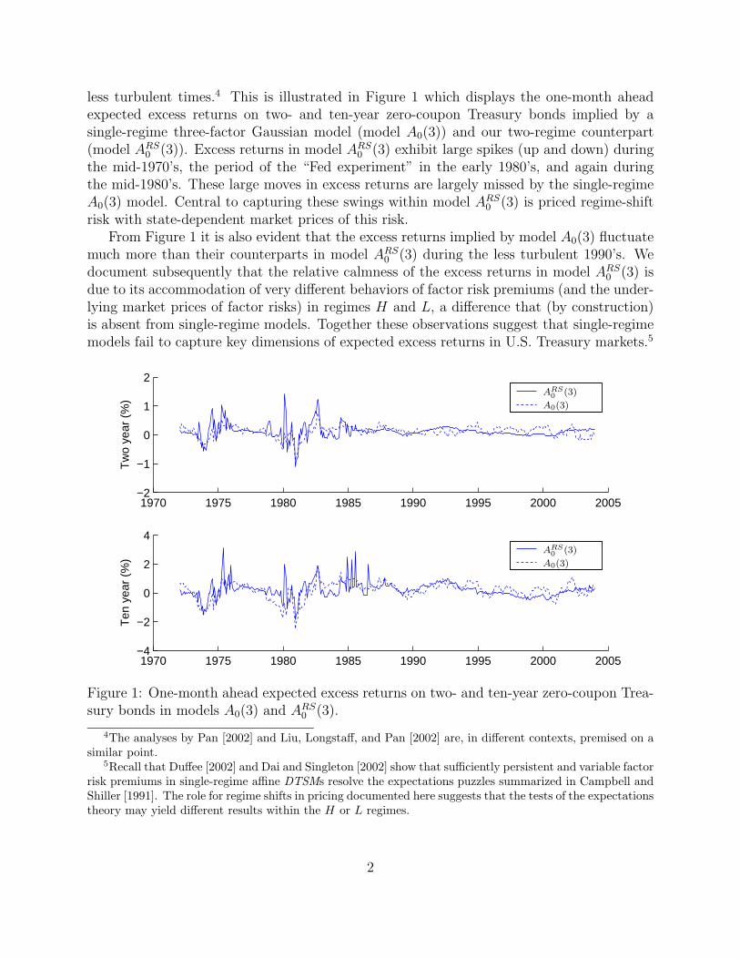
less turbulent times.4 This is illustrated in Figure 1 which displays the one-month aheadexpected excess returns on two- and ten-year zero-coupon Treasury bonds implied by asingle-regime three-factor Gaussian model (model A0(3)) and our two-regime counterpart(model ARS

0 (3)). Excess returns in model ARS0 (3) exhibit large spikes (up and down) during

the mid-1970’s, the period of the “Fed experiment” in the early 1980’s, and again duringthe mid-1980’s. These large moves in excess returns are largely missed by the single-regimeA0(3) model. Central to capturing these swings within model ARS

0 (3) is priced regime-shiftrisk with state-dependent market prices of this risk.

From Figure 1 it is also evident that the excess returns implied by model A0(3) fluctuatemuch more than their counterparts in model ARS

0 (3) during the less turbulent 1990’s. Wedocument subsequently that the relative calmness of the excess returns in model ARS

0 (3) isdue to its accommodation of very different behaviors of factor risk premiums (and the under-lying market prices of factor risks) in regimes H and L, a difference that (by construction)is absent from single-regime models. Together these observations suggest that single-regimemodels fail to capture key dimensions of expected excess returns in U.S. Treasury markets.5

1970 1975 1980 1985 1990 1995 2000 2005−2

−1

0

1

2

Tw

o ye

ar (

%)

1970 1975 1980 1985 1990 1995 2000 2005−4

−2

0

2

4

Ten

yea

r (%

) A0(3)

A0(3)

ARS0

(3)

ARS0

(3)

Figure 1: One-month ahead expected excess returns on two- and ten-year zero-coupon Trea-sury bonds in models A0(3) and ARS

0 (3).

4The analyses by Pan [2002] and Liu, Longstaff, and Pan [2002] are, in different contexts, premised on asimilar point.

5Recall that Duffee [2002] and Dai and Singleton [2002] show that sufficiently persistent and variable factorrisk premiums in single-regime affine DTSMs resolve the expectations puzzles summarized in Campbell andShiller [1991]. The role for regime shifts in pricing documented here suggests that the tests of the expectationstheory may yield different results within the H or L regimes.

2

Where the state dependence of the market price of regime-shift risk (equivalently, statedependence of πP) appears to matter is in modeling the persistence of regimes. A standardresult in the empirical literature on regime-switching models of interest rates with constantπP (e.g., Ang and Bekaert [2002b] and Bansal and Zhou [2002]) is that πPHH ≫ πPHL andπPLL ≫ πPLH ; i.e., both regimes are highly persistent. With state-dependent πP

t , we replicatethe finding that E[πPLL

t ] ≫ E[πPLHt ]. On the other hand, though we still find that E[πPHH

t ]is larger than E[πPHL

t ], the difference is not nearly as large as in models with constant πP.In other words, in the presence of priced, state-dependent regime-shift risk, high volatilityregimes are less persistent than low volatility regimes. Importantly, this asymmetry is equallypresent in a descriptive model of Treasury yields, suggesting that models (descriptive orpricing) that impose a constant πP are missing an empirically important asymmetry in thecyclical behavior of interest rates.

In developing our model we build upon a growing literature on discrete-time DTSMs byextending the Gaussian, discrete-time DTSMs in Bekaert and Grenadier [2001], Ang andPiazzesi [2003], and Gourieroux, Monfort, and Polimenis [2002] to allow for multiple regimesand priced regime-shift risk.6 This is accomplished by overlaying a switching regime processon the conditional distribution of the risk factors. However, rather than adopting Hamilton[1989]’s convention of specifying the distribution of the state conditional on the future regime,we condition on the current regime. Under our convention, all of the conditioning variablesat date t reside in agents’ date t information set, which includes knowledge of the currentregime. This leads to an intuitive interpretation of the components of agents’ pricing kernelthat parallels standard formulations in the continuous-time literature.

Our analysis of a Gaussian DTSM is complementary to Bansal and Zhou [2002]’s studyof an (approximate) discrete-time “CIR-style” DTSM with regime shifts. Model ARS

0 (3)extends their framework by allowing for state-dependent πP

t (Bansal and Zhou assumedthat πP

t = constant), and priced regime-shift risk (they assumed that the market price ofregime-shift risk is zero).7 Furthermore, the added flexibility in the correlation structure ofthe risk factors in model ARS

0 (3) allows us to replicate the well known hump in the termstructure of volatility, and to explore the regime dependence of the shape of this hump. Theassumption of mutually independent, mean-reverting factors in CIR-style models essentiallyforces downward sloping term structures of volatility in all regimes.

In a concurrent study, with a different objective, Ang and Bekaert [2005] also examine aregime-switching Gaussian DTSM.8 They assume that the regime-shift risk is not priced, πP

t

is constant, and the historical rates of mean reversion of the risk factors are the same across

6To the extent that changes in regimes are related to business-cycle developments, multiple switches withina monthly, or even a quarterly, time frame seem unlikely. Therefore, we see little cost to a discrete-timeframework, with the obvious benefit of being able to link our results directly with the descriptive literatureon regime shifts in the distributions of interest rates.

7As we explain more formally below, neither of our models is nested within the other with regard to thespecifications of the market price of factor risks.

8In other related studies, Wu and Zeng [2003] derive a general equilibrium, regime-switching model,building upon the one-factor CIR-style model of Naik and Lee [1997], with constant πP. Veronesi and Yared[2000] develop an equilibrium model of the term structure with regime shifts and constant πQ = πP.

3

regimes. Model ARS0 (3) relaxes all of these assumptions thereby facilitating an exploration

of the state dependence of πPt and of the contributions of the market prices of regime-shift

and factor risks to expected excess returns.The remainder of this paper is organized as follows. Section 2 develops our model and

derives the arbitrage-free bond pricing relations in the presence of regime shifts. We alsocompare the nature of the various market prices of risk in our setup to those in previousstudies. The likelihood function that is used in estimation is derived in Section 3. Section 4describes the data, presents the estimates of our models, and interprets the results. Thecontributions of the regime-shift and factor risks to expected excess returns are explored inmore depth in Section 5. Finally, concluding remarks are presented in Section 6.

2 A Regime-Switching, Gaussian DTSM

In formulating a DTSM for econometric analysis, there is an inherent trade-off between therichness of one’s model and the computational complexity that arises in both pricing andestimation. These trade-offs are compounded in our setting by the introduction of multipleregimes for the state vector Y . Just as in the literature on single-regime affine DTSMs,we proceed by parameterizing the risk-neutral distribution of Y so as to assure closed-formsolutions for bond prices, and then overlay flexible specifications of the market prices of riskto describe the historical distribution of bond yields. This construction also highlights thesources of the added flexibility in our formulation of a regime-switching DTSM relative torecent alternative formulations in the literature.

We assume that there are S + 1 “regimes” that govern the dynamic properties of theN -dimensional state (factor) vector Y . Formally, the joint process (Y, s) is modelled as amarked point process. Heuristically, the regime variable st may be thought of as a (S + 1)-state Markov process, with the risk-neutral (hereafter denoted by Q) probability of switchingfrom regime st = j to regime st+1 = k given by πQjk

t , 0 ≤ j, k ≤ S, with∑S

k=0 πQjkt = 1, for

all j. Agents are presumed to know the current and past histories of both the state vector andthe regime the economy is in. Thus expectations EQ

t [·] are conditioned on the informationset It generated by Yt−ℓ, st−ℓ : ℓ ≥ 0. We use the notation EQ

t [·|st = j] in cases where wewish to highlight the current value of st ∈ It, and use the notation EQ(j)[·] to denote theunconditional mean of a random variable under the assumption of a single-regime economygoverned by the parameters of regime j.9

The Markov process governing regime changes is assumed to be conditionally independentof the Y process. In addition, fQ(Yt+1|Yt−ℓ : ℓ ≥ 0; st = j, st+1 = k) = fQ(Yt+1|Yt−ℓ : ℓ ≥0; st = j). This differs from (our pricing counterpart to) Hamilton [1989]’s formulation wherefQ(Yt+1|Yt−ℓ : ℓ ≥ 0; st = j, st+1 = k) = fQ(Yt+1|Yt−ℓ : ℓ ≥ 0; st+1 = k). As the length of aunit of time shrinks toward zero (in the continuous time limit), these two formulations are

9In adopting this notation we are presuming that the unconditional means in each regime are finite underQ. For our empirical implementation, one of the roots of the mean reversion matrix indicates that Y isborderline non-stationary under Q. This finding is of limited practical relevance for our analysis, since wefocus on conditional moments under P and Q and unconditional moments under P (which are all finite).

4

equivalent. We adopt our discrete-time formulation for comparability with the developmentof continuous-time models, and for the natural interpretation of the market prices of riskthat it yields (see below).10

Given st = j, under Q, Y is assumed to follow the process

Yt+1 = µQjt + Σjǫt+1, (1)

where µQjt ≡ EQ

t [Yt+1|st = j], Σj ≡ Σ(st = j) is a volatility matrix that is regime-dependentbut not dependent on time, and ǫt+1 ∼ N(0, I) is standard normal. It follows that

fQ(Yt+1|Yt−ℓ : ℓ ≥ 0; st = j) ∼ N(µQjt , ΣjΣj′). (2)

Equivalently, the conditional moment generating function (MGF) of Yt+1 is, given st = j,

φQjt (u) ≡ EQ

t

[

eu′Yt+1

∣

∣

∣st = j

]

= eu′µQjt +u′

ΣjΣ

j′u2 , u ∈ RN . (3)

In order to obtain closed-form solutions for zero-coupon bond prices, we parallel Dai andSingleton [2003]’s construction in continuous time and assume

Assumption AQ: Restrictions on the Q distribution of (Y, s):

AµQ: µQj(Yt) = Yt + κQ(θQj − Yt), for constant θQj ∈ RN , j = 0, . . . , S and N ×N constantmatrix κQ with κQ

ij ∈ R.

AπQ: the πQjk are constants, for all j and k.

An implication of assumption AµQ is that the unconditional mean EQ(j)[Yt] differs acrossregimes. On the other hand, to facilitate pricing, the state-dependent component of µQj

t ,κQYt, is assumed to be common across regimes. Assumption AπQ restricts the regime-switching probabilities to be state-independent under Q. Bansal and Zhou [2002] imposeassumption AπQ, but not AµQ in that they allow κQj to be regime-dependent. This takesthem outside of a framework with analytic bond prices and, as such, they study approxi-mate prices using a linearization of their model. Like us, Ang and Bekaert [2005] imposeassumption AQ in its entirety.

The continuously compounded yield on a one-period zero-coupon bond in regime j, rjt ≡

r(Yt, st = j), is assumed to be related to Yt according the affine function

Assumption Ar: rjt = δj

0 + δ′Y Yt.

Under assumption Ar, EQ(j)[rt] differs across regimes, as a result of the regime dependenceof both δj

0 and EQ(j)[Yt]. Bansal and Zhou [2002] constrain δj0 = 0 in both regimes in their

10A similar timing convention was adopted by Cecchetti, Lam, and Mark [1993] in their descriptive studyof equity returns. In the context of descriptive regime-switching models (i.e., observable variables and nopricing), our and Hamilton’s specifications lead to identical likelihood functions, except for the interpretationof the initial values of certain conditional regime probabilities. Once latent factors and pricing are introduced,the interpretations are not the same for reasons discussed subsequently.

5

CIR-style formulation. Allowing for non-zero δj0 seems important in light of the evidence in

Pearson and Sun [1994] (for treasury bonds) and Duffie and Singleton [1997] (for interest rateswaps) that, for their single-regime multi-factor CIR models, a non-zero δ0 was essential tofitting the term structure. With regard to the state-dependent component of rj

t we constrainthe “loadings” δY on Yt to be the same across regimes to facilitate bond pricing. Bansal andZhou’s model is more flexible on this dimension in that δj

Y is regime-dependent owing to thevolatility coefficient in their approximate CIR process changing across regimes.11

These assumptions give rise to closed-form solutions for zero-coupon bond prices.12 Specif-ically, letting Dt,n ≡ Dn(Yt, st) denote the time-t price for a zero-coupon bond with maturityof n periods, and Dj

t,n denote the price when the current regime is st = j, we have:

Proposition 1 (Zero-Coupon Bond Prices) Assuming that Yt+1 follows the process (1)and assumptions AµQ, AπQ, and Ar hold, zero-coupon bond prices are given by

Djt,n = e−A

jn−B′

nYt , (4)

where,

Ajn+1 = δj

0 + (κQθQj)′Bn − 1

2B′

nΣjΣj′Bn − log

(

S∑

k=0

πQjke−Akn

)

, (5)

Bn+1 = δY + Bn − κQ′Bn, (6)

with initial conditions: Aj0 = 0 and B0 = 0.

Proof: Substituting (4) into the risk-neutral pricing equation

Djt,n+1 = EQ

t

[

e−rjt Dt+1,n

∣

∣

∣st = j

]

yields

e−Ajn+1

−B′

n+1Yt = EQ

t

[

e−rjt Dt+1,n|st = j

]

= e−rjt

S∑

k=0

πQjkEQt

[

Dkt+1,n|st = j

]

= e−rjt

S∑

k=0

πQjke−AknEQ

t

[

e−B′

nYt+1 |st = j]

= e−rjt

[

S∑

k=0

πQjke−Akn

]

e−B′

nµQjt + 1

2B′

nΣjΣj′Bn .

11This is a second contributing factor (besides the regime dependence of κQj) to their use of approximationsin pricing bonds.

12More precisely, the dependence of bond yields on Y is known analytically, up to a set of coefficients thatsolve the recursion equations. These equations can be solved essentially instantaneously.

6

Equations (5) and (6) are necessary and sufficient for the above equation to hold for anyYt and st = j. It is easy to check that Aj

0 = 0, B0 = 0, Aj1 = δj

0, and B1 = δY satisfythe recursion. Thus, the recursion can start either at n = 0 or at n = 1. When n denotesmaturities in months, the annualized yields are given by

Rjt,n = aj

n + b′nYt =Aj

n

n/12+

B′n

n/12Yt. (7)

To complete the specification of our model it remains to specify the distribution of(Yt+1, st+1) conditional on It under the historical measure, P. The conditional distributionsof (Yt+1, st+1) under P and Q are linked by the Radon-Nikodym derivative (dP/dQ)t,t+1.

13

Equivalently, under the assumption of no arbitrage opportunities, they are linked by thepricing kernel Mt,t+1 = M(Yt, st; Yt+1, st+1) underlying the time-t valuation of payoffs atdate t + 1, as (dP/dQ)t,t+1 = 1/[ertMt,t+1]. To accommodate both regime-shift and factorrisks we assume that (dP/dQ)t,t+1 is given by

(

dP

dQ

)

t,t+1

= eΓt,t+1−1

2Λ′

tΛt+Λ′

tΣ−1t (Yt+1−µ

Qt ) = eΓt,t+1 × eΛ′

tΣ−1t Yt+1

φQt ((Σ′

t)−1Λt)

, (8)

where Γt,t+1 = Γ(Yt, st; st+1) is the market price of regime-shift (MPRS) risk from st to st+1,Λt = Λ(Yt, st) is the market price of factor (MPF ) risk, and φQ

t ((Σ′t)

−1Λt) is the MGF ofYt+1 under Q evaluated at (Σ′

t)−1Λt. The Radon-Nikodym derivative depends implicitly on

the regimes (st, st+1), because agents know both the regime st+1 and the regime from whichthey have transitioned, st. As will be discussed in more detail, dependence on st+1 enterssolely through the MPRS risk Γt,t+1. The MPF risk, on the other hand, takes a form thatparallels its counterpart in a continuous-time Gaussian DTSM . For later development, wedefine Γjk

t ≡ Γ(Yt, st = j; st+1 = k) and Λjt ≡ Λ(Yt, st = j).

For P to be a well-defined probability measure we require that

1 = EQt [(dP/dQ)t,t+1]

= EQt [eΓt,t+1|st = j] =

S∑

k=0

πQjkeΓjkt , 0 ≤ ∀j ≤ S.

(9)

Since the regime switching probabilities under P are given by

πPjkt ≡ Et

[

1st+1=k|st = j]

= πQjkeΓjkt , (10)

the condition in (9) is equivalent to∑S

k=0 πPjkt = 1.

The conditional distribution of Yt+1 under P is fully characterized by its MGF :

φPjt (u) ≡ Et

[

eu′Yt+1 |st = j]

= EQt

[

eu′Yt+1(dP/dQ)t,t+1|st = j]

=φQj

t ((Σj′)−1Λjt + u)

φQjt ((Σj′)−1Λj

t)= eu′(µ

Qjt +ΣjΛj

t)+u′Σ

jΣ

j′u2 , u ∈ RN .

(11)

13The P and Q distributions are related according to P(dYt+1, st+1|It) = (dP/dQ)t,t+1Q(dYt+1, st+1|It).

7

Thus, this distribution is also Gaussian with conditional mean

µPt = µQ

t + ΣtΛt, (12)

and variance ΣtΣ′t. Moreover, the P distribution of (Y, s) inherits the property from the Q

distribution that Y and s are conditionally independent processes.The pricing kernel implied by our choice of Radon-Nikodym derivative in (8) is:

Mt,t+1 = e−rt−Γt,t+1−1

2Λ′

tΛt−Λ′

tΣ−1t (Yt+1−µP

t ). (13)

No arbitrage requires that

e−rjt = Et[Mt,t+1|st = j] = e−r

jt Et[(dQ/dP)t,t+1|st = j], (14)

which is guaranteed by the requirement that∑S

k=0 πQjk = 1.To motivate our labelling of the component Λt of the pricing kernel M as the market

prices of factor risks, consider the security with payoff e−b′Yt+1 , which has exposure only tofactor risks at date t + 1. Its price is

P jt = e−r

jt EQ

t [e−b′Yt+1 |st = j] = e−rjt e−b′µ

Qjt + 1

2b′ΣjΣj′b, (15)

and its P-expected payoff is Et[e−b′Yt+1 ] = e−b′µ

Pjt + 1

2b′ΣjΣj′b in regime st = j. Therefore, the

log expected return for this security, in excess of the one period zero-coupon bond yield, is14

logEt[e

−b′Yt+1 |st = j]

P jt

− rjt = −b′ΣjΛj

t . (16)

Since b′Σj is the “risk exposure” or volatility of the security associated with the factor risk,the MPF risk in regime st = j, Λj

t , gives the excess log expected return per unit of factorrisk exposure.

Turning to the component Γt,t+1, consider a security with payoff 1st+1=k, which hasexposure only to the risk of shifting to regime k at date t + 1. Conditional on the current

regime st = j, its risk-neutral expected payoff is πQjk, and its current price is P jt = e−r

jt πQjk.

Thus, its excess log expected return is given by

logEt[1st+1=k|st = j]

P jt

− rjt = Γjk

t . (17)

That is, Γjkt,t+1 is naturally defined as the MPRS risk from regime j to regime k.

14For intuitive interpretation of the market prices of risks, log expected returns in excess of the one periodshort rate provide a more convenient platform than the conventionally defined, expected excess log returns.The latter, which are related to the market prices of risks in qualitatively very similar manners, will beexamined in Section 5.

8

Importantly, assumption AµQ does not constrain the state or regime dependence of µP.Given our parametrization of µQj

t and the regime dependence of Σj, we can match any desiredstate and regime dependence of µPj

t under P,

µPjt = µQj

t + ΣjΛjt , 0 ≤ j ≤ S, (18)

by appropriate choice of the market prices of factor risks, Λjt . In our parametric DTSM, we

extend Duffee [2002]’s essentially affine, Gaussian model to the case of multiple regimes byassuming that

Λjt =

(

Σj)−1 (

λj0 + λj

Y Yt

)

. (19)

Duffee [2002] and Dai and Singleton [2002] found that A0(3) models with MPF risks givenby (19) (without the regime index) were able to match many features of historical expectedexcess returns on bonds. The regime independence of κQ (assumption AµQ) requires that

κQ = κPL + λLY = κPH + λH

Y . (20)

To take advantage of the maximal flexibility allowed by this restriction, we set κPL, λLY , and

λHY as free parameters in our model. Consequently, κPH as well as κQ are derived parameters.

Similarly assumption AπQ does not restrict the state dependence of πPjkt . Given the πQjk,

by appropriate choice of the Γjkt , we can match any desired state dependence of the πPjk

t ,subject to the constraint that

∑S

k=0 πPjkt = 1. Following Gray [1996], Boudoukh, Richardson,

Smith, and Whitelaw [1999], and many subsequent studies, we assume that (for the two-regime case)

πPjkt =

1

1 + eηjk0

+ηjkY

Yt

, πPjjt = 1 − πPjk

t , j 6= k. (21)

Consequently, the MPRS risks are

Γjkt = log

(

πPjkt

πQjk

)

, ∀ j, k. (22)

The unknown parameters to be estimated are the (constant) risk-neutral regime-shift prob-abilities πQjk, ηjk

0 , and ηjkY . Unlike in descriptive regime-switching models for interest rates,

the elements of πP in our DTSM depend directly on the latent risk factors Y (rather thanon the yields themselves).

Our specification (13) of the pricing kernel M, and the associated market prices of risk,extends the literature on regime-switching models for interest rates along several importantdimensions. As in Naik and Lee [1997] and Bansal and Zhou [2002], we assume that the πQjk

are constants (assumption AπQ). However, these studies also assume that regime-shift riskis not priced (Γjk

t = 0). Regime-shift risk is also not priced (and the πQjk are constants) inthe regime-switching Gaussian model used by Ang and Bekaert [2005] in their study of realreturns. The state dependence of the Γjk

t implied by (21) and (22) is key to achieving ourobjective of an improved understanding of the nature of market prices of risk, and regime-shift risk in particular. The assumption that Γjk

t = 0 means that the state and regime

9

dependence of Λjt and Σj (the volatility matrix of Y ) must explain the time-series properties

of expected excess returns. By allowing for priced regime-shift risk, we have an additionalregime-dependent channel through which risk preferences can affect expected excess returns.

Our formulation of the market prices of factor risks shares with Bansal and Zhou [2002]the features that Λt is both state- and regime-dependent. Where we differ is in our focuson different members of the affine family of term structure models. They focus on an ap-proximate CIR style model, and assume that the market prices of risk are proportional tofactor volatilities (a “completely affine” model). Though our within-regime volatilities areconstant (due to the Gaussian framework), our market prices of risk depend directly onthe state variables according to (19). Within single-regime models, the latter “essentiallyaffine” models have been found to fit the dynamic properties of yield curves much betterthan completely affine CIR-style models (e.g., Duffee [2002], Dai and Singleton [2002]).

The specification (19) of Λt allows both the constant term (λj0) and the coefficients in the

state-dependent term (λjY ) to change across regimes. Ang and Bekaert [2005] also allow their

counterpart to λj0 to change across regimes for one of their two latent factors. However, for

this factor, they assume that λjY = 0. Further, they assume that the market price of inflation

risk is zero at all dates and in all regimes. It follows that, for both of these factors, the MPFshave no effect on the time series properties of excess returns within regimes.15 For their thirdfactor (also latent), the market prices of risk are state-, but not regime-dependent. As such,they constrain the degree of persistence of all three of their risk factors (the state-dependentcomponents of the conditional mean of Yt+1) to be the same across regimes. Given our focuson the relations between the time series properties of excess returns and the market pricesof factor and regime-shift risks, we allow the components of λj

Y to be non-zero and regime-dependent for all three factors, in order to give maximal flexibility to the market prices offactor risks in our analysis.

A potential weakness of our Gaussian DTSM, relative to say multiple-regime versions ofAM(N) DTSMs, with M > 0, is that the within-regime conditional variances of the Y ’s areconstants. However, our experience with single-regime affine DTSMs is that the conditionalvolatility in bond yields induced by conditional volatility in the Y ’s is, in fact, very smallrelative to the volatility of excess returns. Furthermore, by overlaying regime shifts on top ofa Gaussian state vector we introduce stochastic volatility into our DTSM, perhaps at least tothe same degree as in square-root processes. Even in the case of constant πP, the conditionalvariances of bond yields will be time varying due to the possibility of regime shifts. Thisis the only source of time-varying volatility in Gaussian models that assume that πP is aconstant matrix (e.g., Ang and Bekaert [2005]). With the introduction of state-dependentπP (equivalently, state-dependent Γjk), we allow for an important additional source of time-varying volatility that is absent from extant single- and multiple-regime Gaussian models.

Additionally, assumptions AπQ and (22) imply that our model cannot accommodatestate-dependent regime-shift risk that is not priced. This is a consequence of the fact that,since the πQjk are not state-dependent, any state dependence in the πPjk

t is inherited from

15The factor risk component of the expected excess returns, as shown in (37), implies that within regimes,time varying expected excess returns result from state-dependent MPF risks.

10

state-dependence of the market prices of regime-shift risks, Γjkt , in our model. We nest the

special cases of πQ and πP being constants, with Γjk being either a non-zero constant (pricedregime-shift risk) or zero (non-priced regime-shift risk). However, our formulation does notnest the case of state-dependent πP

t with Γjkt = 0. Nevertheless, we view the accommodation

of state-dependent πP and rich regime dependence of Λjt as potentially important extensions

of the literature on A0(3) models that are worthwhile exploring empirically.Finally, a notable difference between our formulation and that in Bansal and Zhou [2002]

and Ang and Bekaert [2005] is that we have assumed that (Λjt , Γ

jkt ) ∈ It, consistent with the

continuous-time regime-switching model developed in Dai and Singleton [2003]. In contrast,using our notation for the one-factor case, these authors adopted the pricing kernel

Mt,t+1 = exp

[

−rf,t − (λst+1)2Yt

2− λst+1ǫt+1

]

, (23)

in which λst+1 depends on st+1. In our formulation, the components Λjt and Γjk

t can bedirectly interpreted as market prices of risk. On the other hand, under the formulation (23),λst+1 is not the MPF risk, since it is not in It. The MPF risk depends on both λst+1 and theregime-switching probabilities πPjk.16

3 Maximum Likelihood Estimation

Given the Gaussian structure of the risk factors, we proceed with maximum likelihood (ML)estimation of the regime-switching DTSMs. Following common practice (e.g., Chen andScott [1995], Duffie and Singleton [1997]), we assume that the yields on a collection of Nzero-coupon bonds are priced without error, and the yields on a collection of M zero-couponbonds are priced with error.

Let Rt be the vector of yields for the bonds priced exactly by the model. In regimest = j, Rt = aj + bY j

t , where aj is the N × 1 regime-dependent vector, b is the N × Nregime-independent matrix of factor loadings, and Y j

t is the N × 1 vector of state variablesimplied by the model. Inverting for fitted yields we obtain

Y jt = b−1(Rt − aj). (24)

Conditional on st = j and st+1 = k, we have

Rt+1 = ak + bY kt+1 = ak + bµPj

t + bΣjǫt+1

= Rt + (ak − aj) + κPj(θPj − Rt) + Σjǫt+1, (25)

16More precisely, in their setting, the excess log expected return for a security with regime-independent,time-(t + 1) payoff of e−bYt+1 is given by

log

∑Sk=0

πPjke−bµPk

t+

Yt

2bΣk

Σkb

∑Sk=0

πPjke−bµPk

t+

Yt

2bΣkΣkb+bλkYt

.

11

where µPjt = Yt + κPj(θPj − Yt), κPj = bκPj b−1, θPj = aj + bθPj, and Σj = bΣj. It follows that

f(Rt+1|Rt, st = j, st+1 = k)

=e−

1

2(Rt+1−Rt−(ak−aj)−κj(θj−Rt))′[ΣjΣj′]−1(Rt+1−Rt−(ak−aj)−κj(θj−Rt))

√

(2π)N

∣

∣

∣ΣjΣj′

∣

∣

∣

. (26)

Notice that f(Rt+1|Rt, st = j) is obtained by integrating out the dependence of (26) on st+1,so conditioning only on st = j (and Rt) gives a mixture-of-normals distribution.

The remaining M yields used in estimation are denoted by Rt, with corresponding load-ings aj and b when st = j:

Rt = aj + bY jt + uj

t = (aj − bb−1aj) + bb−1Rt + ujt , (27)

where ut is i.i.d. with zero mean and volatility Ωj. Thus, the conditional density for Rt+1,conditional on Rt+1, st = j and st+1 = k, is given by

f(Rt+1|Rt+1, st = j, st+1 = k)

=e−

1

2(Rt+1−(ak−bb−1ak)−bb−1Rt+1)′[ΩkΩk′]−1(Rt+1−(ak−bb−1ak)−bb−1Rt+1)

√

2π |ΩkΩk′|.

(28)

To construct the likelihood function for the data, we introduce the econometrician’sinformation set Jt = Rτ , Rτ , τ ≤ t ⊂ It, and let Qj

t = f(st = j|Jt) be the probability ofregime j given Jt. Define the following matrices:

Qt =[

f(st = 0|Jt) f(st = 1|Jt)]

,

fRt,t+1 =

[

f(Rt+1|Rt, st = 0, st+1 = 0) f(Rt+1|Rt, st = 0, st+1 = 1)

f(Rt+1|Rt, st = 1, st+1 = 0) f(Rt+1|Rt, st = 1, st+1 = 1)

]

,

fut,t+1 =

[

f(Rt+1|Rt+1, st+1 = 0) f(Rt+1|Rt+1, st+1 = 1)

f(Rt+1|Rt+1, st+1 = 0) f(Rt+1|Rt+1, st+1 = 1)

]

.

Using this notation, the conditional density of observed yields is

f(Rt+1, Rt+1|Jt) =∑

j

f(Rt+1, Rt+1|Jt, st = j)Qjt

=∑

j,k

f(Rt+1, Rt+1|Jt, st = j, st+1 = k)Qjtπ

Pjkt

=∑

j,k

f(Rt+1|Rt, st = j, st+1 = k)Qjtπ

Pjkt f(Rt+1|Rt+1, st+1 = k).

12

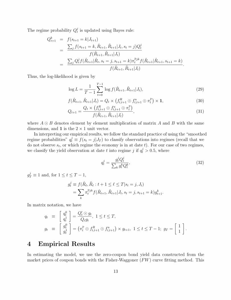
The regime probability Qjt is updated using Bayes rule:

Qkt+1 = f(st+1 = k|Jt+1)

=

∑

j f(st+1 = k, Rt+1, Rt+1|Jt, st = j)Qjt

f(Rt+1, Rt+1|Jt)

=

∑

j Qjtf(Rt+1|Rt, st = j, st+1 = k)πPjk

t f(Rt+1|Rt+1, st+1 = k)

f(Rt+1, Rt+1|Jt).

Thus, the log-likelihood is given by

log L =1

T − 1

T−1∑

t=0

log f(Rt+1, Rt+1|Jt), (29)

f(Rt+1, Rt+1|Jt) = Qt ×(

fRt,t+1 ⊙ fu

t,t+1 ⊙ πPt

)

× 1, (30)

Qt+1 =Qt ×

(

fRt,t+1 ⊙ fu

t,t+1 ⊙ πPt

)

f(Rt+1, Rt+1|Jt), (31)

where A ⊙ B denotes element by element multiplication of matrix A and B with the samedimensions, and 1 is the 2 × 1 unit vector.

In interpreting our empirical results, we follow the standard practice of using the “smoothedregime probabilities” qj

t ≡ f(st = j|JT ) to classify observations into regimes (recall that wedo not observe st, or which regime the economy is in at date t). For our case of two regimes,we classify the yield observation at date t into regime j if qj

t > 0.5, where

qjt =

gjt Q

jt

∑

k gkt Q

kt

, (32)

gjT ≡ 1 and, for 1 ≤ t ≤ T − 1,

gjt ≡ f(Rℓ, Rℓ : t + 1 ≤ ℓ ≤ T |st = j, Jt)

=∑

k

πPjkt f(Rt+1, Rt+1|Jt, st = j, st+1 = k)gk

t+1.

In matrix notation, we have

qt ≡[

q0t

q1t

]

=Q′

t ⊙ gt

Qtgt

, 1 ≤ t ≤ T,

gt ≡[

g0t

g1t

]

=(

πPt ⊙ fR

t,t+1 ⊙ fut,t+1

)

× gt+1, 1 ≤ t ≤ T − 1; gT =

[

11

]

.

4 Empirical Results

In estimating the model, we use the zero-coupon bond yield data constructed from themarket prices of coupon bonds with the Fisher-Waggoner (FW ) curve fitting method. This

13

method, together with Unsmoothed Fama-Bliss (UFB), McCulloch-Kwon (MK), SmoothedFama-Bliss (SFB), and Nelson-Siegel-Bliss (NSB), comprise the most popular zero-couponyield estimation methods in the empirical literature.17 One important difference across thesemethods is the resulting degree of smoothness of the estimated term structure data. At oneextreme, the USB method iteratively extracts forward rates from coupon bond prices bybuilding a piece-wise linear discount rate function, and the implied discount rates exhibitkinks at the maturities of the coupon bonds used. At the other extreme, the NSB and theSFB methods approximate the discount rates with exponential functions of time to maturityand the resulting forward rate function is differentiable to infinite order.

The FW method seems to occupy a desirable middle ground. It is based on a cubicspline, similar to the MK method.18 A large number of knots (as many as 50 to 60 knots)are used when minimizing the fitting errors, and then a penalty is imposed on the excessvariability of yields induced by the flexibility of the spline. In contrast to the kinky USByield curves, the FW method generates a smooth term structure with a continuous firstderivative. In contrast to the possibly over-smoothed NSB and SFB data, the flexibilityof the 50 to 60 knot points allows the FW data to better track the many small dips andhumps in the underlying coupon bond yields.

We estimate a two-regime, three-factor (N = 3) model, ARS0 (3), using the FW monthly

data on U.S. Treasury zero-coupon bond yields for the period 1972 to 2003.19 The vectorR includes the yields on bonds with maturities of 6, 24, and 120 months, and M = 1 withR chosen to be the yield on the 60-month bond. The two regimes are denoted L and H,corresponding to “low” and “high” values of the diagonal entries of Σj (see below).

In parameterizing model ARS0 (3), we impose several normalizations. Analogous to the

normalizations imposed in Dai and Singleton [2000] for single-regime affine DTSMs, in regimeL, we set the annualized volatility

√12ΣL to an identity matrix, κPL to a lower triangular

matrix, and θPL to zero. The normalization of ΣL is needed, because we have allowedδY to be free and the factors Y are latent. Second, in regime H, ΣH was set to a lowerdiagonal matrix, because the Brownian motions in regime H can be rotated independentlyof any rotations on the Brownian motions in regime L. Beyond these normalizations, therestrictions κQH = κQL ≡ κQ and δH

Y = δLY = δY were imposed so that zero-coupon bonds

are priced in closed form. Consequently κPL + λLY = κPH + λH

Y .

17Bliss [1997] provides a more detailed description of these methods. The Unsmoothed Fama-Bliss methodis documented in Fama and Bliss [1987]. The McCulloch-Kwon method is a modified version of the McCullochmethod (McCulloch [1975]). The Fisher-Waggoner method (Waggoner [1997]) is a modified version of theFisher-Nychka-Zervos method (Fisher, Nychka, and Zervos [1995]). The Nelson-Siegel-Bliss method wasoriginally labeled the extended Nelson-Siegel method in Bliss [1997]. The original Nelson-Siegel method(Nelson and Siegel [1987]) has only four free parameters. The Nelson-Siegel-Bliss method has five parametersfree so as to provide a better fit for longer maturities (Bliss [1997]).

18In the MK method a cubic spline is used to approximate the discount function, and the spline isestimated with ordinary least squares. The FW method uses a cubic spline to approximate the forward ratefunction itself.

19The FW data is generated using “The Bliss Term Structure Generating Programs” with the filtered“long data set”, which filters out bonds with option features and liquidity problems, but otherwise containsall eligible issues. See Bliss [1997].

14

Even with these normalizations/constraints, the resulting maximally flexible ARS0 (3)

model (with restrictions for analytical pricing) involves a high dimensional parameter space:there are 56 parameters in

δL0 , δH

0 , δY , κPL, θPH , ΣH , λL0 , λL

Y , λH0 , λH

Y , ΩL, ΩH , πQ, ηLH0 , ηLH

Y , ηHL0 , ηHL

Y .

To facilitate numerical identification of the free parameters, we imposed several additionalover-identifying restrictions. The model, together with the normalizations, imply that wheneconomy stays in a regime L or H forever, the long-run mean of the short rate is E(L)[rt] = δL

0

and E(H)[rt] = δH0 + δ′Y θPH . Given the challenge of estimating these unconditional means,

we discipline our search procedure by fixing them a priori. Specifically, we use the regimesidentified from the descriptive regime-switching model and compute the sample means forthe one-month Treasury bill yield when the regimes are L (H) for the current month tand months t − ℓ, where ℓ is at least 1. Using these estimates, we fix δL

0 = 5.30%/12 andδH0 + δ′Y θPH = 9.20%/12. Also, after a preliminary exploration of model ARS

0 (3) we setthe parameters κPL(2, 1), ΣH(2, 1), ΣH(3, 1), ΣH(3, 2), λL

Y (1, 1), λLY (2, 1), λL

Y (2, 2), λLY (3, 2),

λH0 (1), λH

0 (2), λH0 (3), λH

Y (1, 3), λHY (2, 3), λH

Y (3, 2), λHY (3, 3), ηLH

Y (2), and ηHLY (1) to 0, because

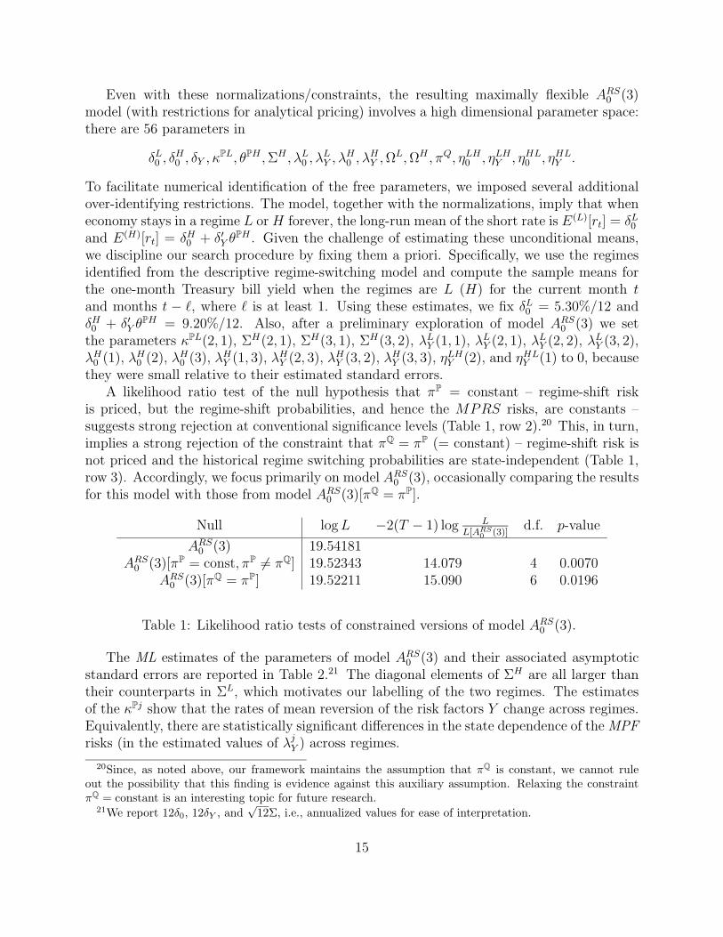
they were small relative to their estimated standard errors.A likelihood ratio test of the null hypothesis that πP = constant – regime-shift risk

is priced, but the regime-shift probabilities, and hence the MPRS risks, are constants –suggests strong rejection at conventional significance levels (Table 1, row 2).20 This, in turn,implies a strong rejection of the constraint that πQ = πP (= constant) – regime-shift risk isnot priced and the historical regime switching probabilities are state-independent (Table 1,row 3). Accordingly, we focus primarily on model ARS

0 (3), occasionally comparing the resultsfor this model with those from model ARS

0 (3)[πQ = πP].

Null log L −2(T − 1) log L

L[ARS0

(3)]d.f. p-value

ARS0 (3) 19.54181

ARS0 (3)[πP = const, πP 6= πQ] 19.52343 14.079 4 0.0070

ARS0 (3)[πQ = πP] 19.52211 15.090 6 0.0196

Table 1: Likelihood ratio tests of constrained versions of model ARS0 (3).

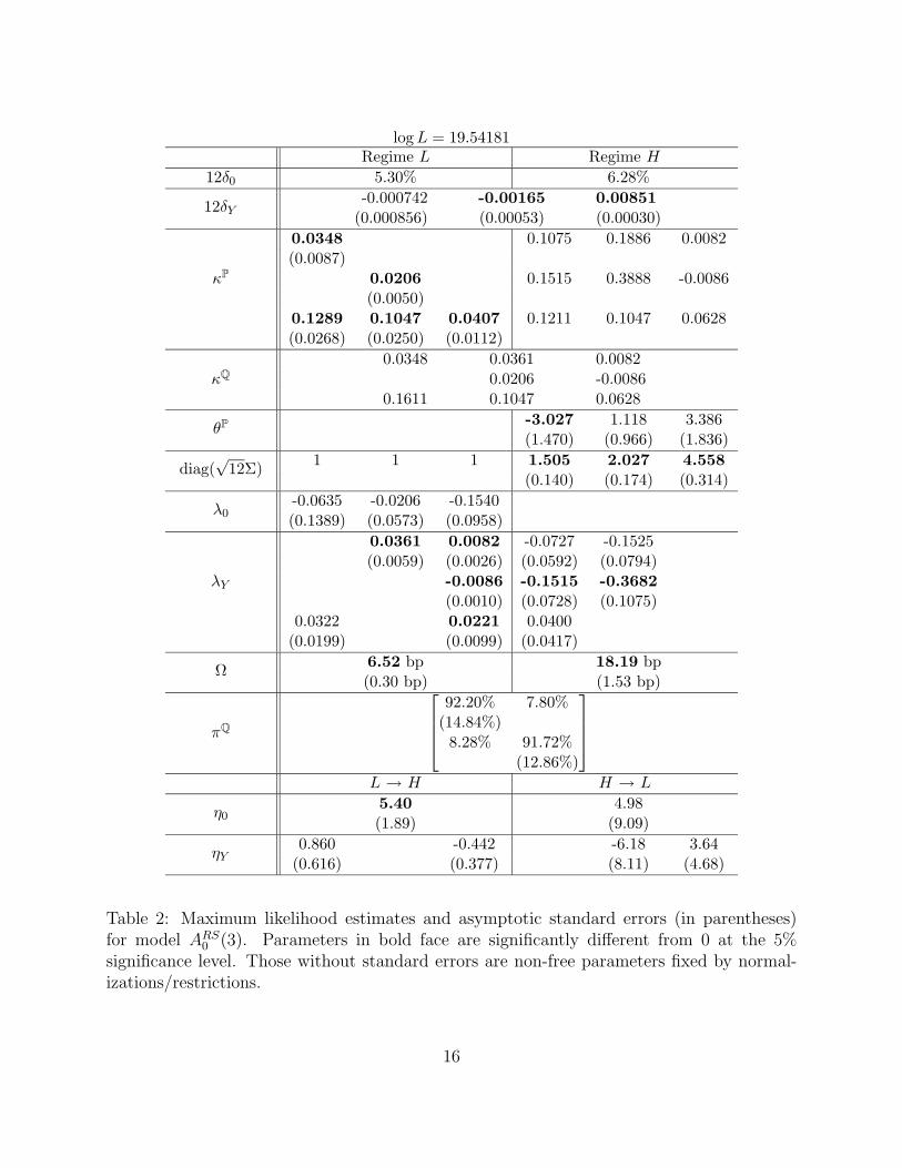
The ML estimates of the parameters of model ARS0 (3) and their associated asymptotic

standard errors are reported in Table 2.21 The diagonal elements of ΣH are all larger thantheir counterparts in ΣL, which motivates our labelling of the two regimes. The estimatesof the κPj show that the rates of mean reversion of the risk factors Y change across regimes.Equivalently, there are statistically significant differences in the state dependence of the MPFrisks (in the estimated values of λj

Y ) across regimes.

20Since, as noted above, our framework maintains the assumption that πQ is constant, we cannot ruleout the possibility that this finding is evidence against this auxiliary assumption. Relaxing the constraintπQ = constant is an interesting topic for future research.

21We report 12δ0, 12δY , and√

12Σ, i.e., annualized values for ease of interpretation.

15

log L = 19.54181Regime L Regime H

12δ0 5.30% 6.28%

12δY-0.000742 -0.00165 0.00851

(0.000856) (0.00053) (0.00030)

0.0348 0.1075 0.1886 0.0082(0.0087)

κP0.0206 0.1515 0.3888 -0.0086(0.0050)

0.1289 0.1047 0.0407 0.1211 0.1047 0.0628(0.0268) (0.0250) (0.0112)

0.0348 0.0361 0.0082κQ 0.0206 -0.0086

0.1611 0.1047 0.0628

θP -3.027 1.118 3.386(1.470) (0.966) (1.836)

diag(√

12Σ)1 1 1 1.505 2.027 4.558

(0.140) (0.174) (0.314)

λ0-0.0635 -0.0206 -0.1540(0.1389) (0.0573) (0.0958)

0.0361 0.0082 -0.0727 -0.1525(0.0059) (0.0026) (0.0592) (0.0794)

λY -0.0086 -0.1515 -0.3682

(0.0010) (0.0728) (0.1075)0.0322 0.0221 0.0400

(0.0199) (0.0099) (0.0417)

Ω6.52 bp 18.19 bp(0.30 bp) (1.53 bp)

πQ

92.20% 7.80%(14.84%)8.28% 91.72%

(12.86%)

L → H H → L

η05.40 4.98(1.89) (9.09)

ηY0.860 -0.442 -6.18 3.64

(0.616) (0.377) (8.11) (4.68)

Table 2: Maximum likelihood estimates and asymptotic standard errors (in parentheses)for model ARS

0 (3). Parameters in bold face are significantly different from 0 at the 5%significance level. Those without standard errors are non-free parameters fixed by normal-izations/restrictions.

16

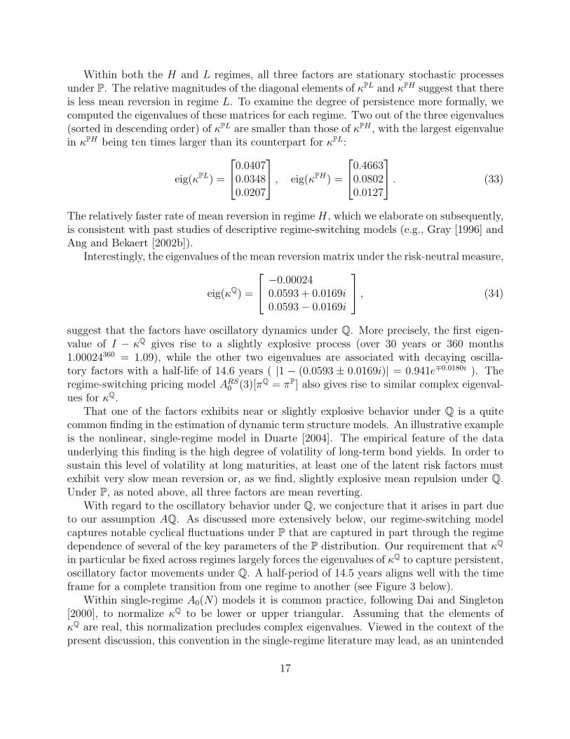
Within both the H and L regimes, all three factors are stationary stochastic processesunder P. The relative magnitudes of the diagonal elements of κPL and κPH suggest that thereis less mean reversion in regime L. To examine the degree of persistence more formally, wecomputed the eigenvalues of these matrices for each regime. Two out of the three eigenvalues(sorted in descending order) of κPL are smaller than those of κPH , with the largest eigenvaluein κPH being ten times larger than its counterpart for κPL:

eig(κPL) =

0.04070.03480.0207

, eig(κPH) =

0.46630.08020.0127

. (33)

The relatively faster rate of mean reversion in regime H, which we elaborate on subsequently,is consistent with past studies of descriptive regime-switching models (e.g., Gray [1996] andAng and Bekaert [2002b]).

Interestingly, the eigenvalues of the mean reversion matrix under the risk-neutral measure,

eig(κQ) =

−0.000240.0593 + 0.0169i0.0593 − 0.0169i

, (34)

suggest that the factors have oscillatory dynamics under Q. More precisely, the first eigen-value of I − κQ gives rise to a slightly explosive process (over 30 years or 360 months1.00024360 = 1.09), while the other two eigenvalues are associated with decaying oscilla-tory factors with a half-life of 14.6 years ( |1 − (0.0593 ± 0.0169i)| = 0.941e∓0.0180i ). Theregime-switching pricing model ARS

0 (3)[πQ = πP] also gives rise to similar complex eigenval-ues for κQ.

That one of the factors exhibits near or slightly explosive behavior under Q is a quitecommon finding in the estimation of dynamic term structure models. An illustrative exampleis the nonlinear, single-regime model in Duarte [2004]. The empirical feature of the dataunderlying this finding is the high degree of volatility of long-term bond yields. In order tosustain this level of volatility at long maturities, at least one of the latent risk factors mustexhibit very slow mean reversion or, as we find, slightly explosive mean repulsion under Q.Under P, as noted above, all three factors are mean reverting.

With regard to the oscillatory behavior under Q, we conjecture that it arises in part dueto our assumption AQ. As discussed more extensively below, our regime-switching modelcaptures notable cyclical fluctuations under P that are captured in part through the regimedependence of several of the key parameters of the P distribution. Our requirement that κQ

in particular be fixed across regimes largely forces the eigenvalues of κQ to capture persistent,oscillatory factor movements under Q. A half-period of 14.5 years aligns well with the timeframe for a complete transition from one regime to another (see Figure 3 below).

Within single-regime A0(N) models it is common practice, following Dai and Singleton[2000], to normalize κQ to be lower or upper triangular. Assuming that the elements ofκQ are real, this normalization precludes complex eigenvalues. Viewed in the context of thepresent discussion, this convention in the single-regime literature may lead, as an unintended

17

consequence, to the inability of single-regime A0(N) models to capture the rich cyclicalpatterns documented here within our ARS

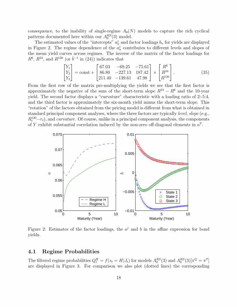
0 (3) model.The estimated values of the “intercepts” aj

n and factor loadings bn for yields are displayedin Figure 2. The regime dependence of the aj

n contributes to different levels and slopes ofthe mean yield curves across regimes. The inverse of the matrix of the factor loadings forR6, R24, and R120 (or b−1 in (24)) indicates that

Y1

Y2

Y3

= const +

67.03 −69.25 −75.6186.80 −227.13 187.42211.40 −139.61 47.98

×

R6

R24

R120

. (35)

From the first row of the matrix pre-multiplying the yields we see that the first factor isapproximately the negative of the sum of the short-term slope R24 − R6 and the 10-yearyield. The second factor displays a “curvature” characteristic with a loading ratio of 2:-5:4,and the third factor is approximately the six-month yield minus the short-term slope. This“rotation” of the factors obtained from the pricing model is different from what is obtained instandard principal component analyses, where the three factors are typically level, slope (e.g.,R120

t −rt), and curvature. Of course, unlike in a principal component analysis, the componentsof Y exhibit substantial correlation induced by the non-zero off-diagonal elements in κP.

0 5 100.05

0.055

0.06

0.065

0.07

0.075

Maturity (Year)

Regime HRegime L

0 5 10−0.01

−0.005

0

0.005

0.01

Maturity (Year)

State 1State 2State 3

a b

Figure 2: Estimates of the factor loadings, the aj and b in the affine expression for bondyields.

4.1 Regime Probabilities

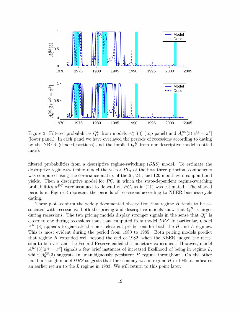
The filtered regime probabilities QHt = f(st = H|Jt) for models ARS

0 (3) and ARS0 (3)[πQ = πP]

are displayed in Figure 3. For comparison we also plot (dotted lines) the corresponding

18

1970 1975 1980 1985 1990 1995 2000 20050

0.5

1ModelDesc

1970 1975 1980 1985 1990 1995 2000 20050

0.5

1ModelDesc

AR

S0

(3)

AR

S0

(3)[π

Q=

πP]

Figure 3: Filtered probabilities QHt from models ARS

0 (3) (top panel) and ARS0 (3)[πQ = πP]

(lower panel). In each panel we have overlayed the periods of recessions according to datingby the NBER (shaded portions) and the implied QH

t from our descriptive model (dottedlines).

filtered probabilities from a descriptive regime-switching (DRS) model. To estimate thedescriptive regime-switching model the vector PCt of the first three principal componentswas computed using the covariance matrix of the 6-, 24-, and 120-month zero-coupon bondyields. Then a descriptive model for PCt in which the state-dependent regime-switchingprobabilities πPC

t were assumed to depend on PCt as in (21) was estimated. The shadedperiods in Figure 3 represent the periods of recessions according to NBER business-cycledating.

These plots confirm the widely documented observation that regime H tends to be as-sociated with recessions: both the pricing and descriptive models show that QH

t is largerduring recessions. The two pricing models display stronger signals in the sense that QH

t iscloser to one during recessions than that computed from model DRS. In particular, modelARS

0 (3) appears to generate the most clear-cut predictions for both the H and L regimes.This is most evident during the period from 1980 to 1985. Both pricing models predictthat regime H extended well beyond the end of 1982, when the NBER judged the reces-sion to be over, and the Federal Reserve ended the monetary experiment. However, modelARS

0 (3)[πQ = πP] signals a few brief instances of increased likelihood of being in regime L,while ARS

0 (3) suggests an unambiguously persistent H regime throughout. On the otherhand, although model DRS suggests that the economy was in regime H in 1985, it indicatesan earlier return to the L regime in 1983. We will return to this point later.

19

1970 1975 1980 1985 1990 1995 2000 20050

0.5

1ModelDesc

1970 1975 1980 1985 1990 1995 2000 20050

0.5

1

πPL

Ht

πPH

Lt

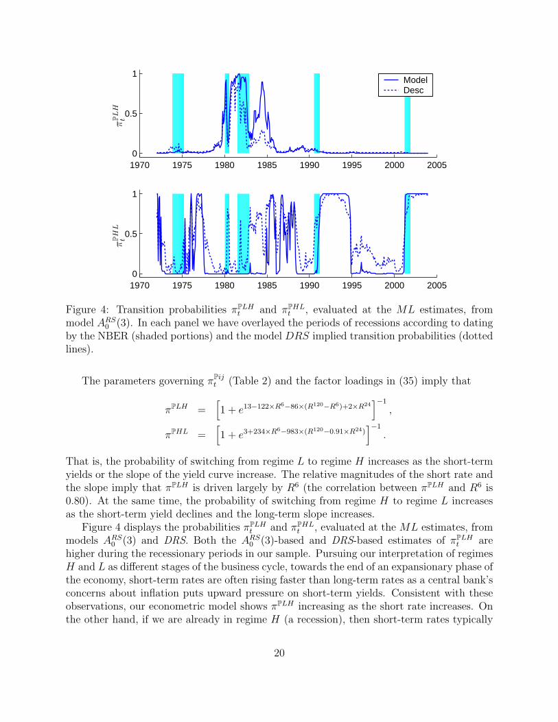
Figure 4: Transition probabilities πPLHt and πPHL

t , evaluated at the ML estimates, frommodel ARS

0 (3). In each panel we have overlayed the periods of recessions according to datingby the NBER (shaded portions) and the model DRS implied transition probabilities (dottedlines).

The parameters governing πPijt (Table 2) and the factor loadings in (35) imply that

πPLH =[

1 + e13−122×R6−86×(R120−R6)+2×R24]−1

,

πPHL =[

1 + e3+234×R6−983×(R120−0.91×R24)]−1

.

That is, the probability of switching from regime L to regime H increases as the short-termyields or the slope of the yield curve increase. The relative magnitudes of the short rate andthe slope imply that πPLH is driven largely by R6 (the correlation between πPLH and R6 is0.80). At the same time, the probability of switching from regime H to regime L increasesas the short-term yield declines and the long-term slope increases.

Figure 4 displays the probabilities πPLHt and πPHL

t , evaluated at the ML estimates, frommodels ARS

0 (3) and DRS. Both the ARS0 (3)-based and DRS-based estimates of πPLH

t arehigher during the recessionary periods in our sample. Pursuing our interpretation of regimesH and L as different stages of the business cycle, towards the end of an expansionary phase ofthe economy, short-term rates are often rising faster than long-term rates as a central bank’sconcerns about inflation puts upward pressure on short-term yields. Consistent with theseobservations, our econometric model shows πPLH increasing as the short rate increases. Onthe other hand, if we are already in regime H (a recession), then short-term rates typically

20

have to come down far enough to induce an expansion. This is consistent with πPHL risingas short-term rates fall and the long-term slope increases.

During the recessionary periods in our sample, πPLH and πPHL tend to move in oppositedirections. That is, when the U.S. economy was in a recession, the conditional probability ofmoving from regime H to regime L was lower. As noted above, πPHL was driven by the short-term rate R6 and the long-term slope. During 1984 the Federal Reserve temporarily tightenedmonetary policy. Then in late 1984 and throughout 1985 there was a monetary easing andconcurrent decline in short-term interest rates. Additionally, the striking decline in U.S.inflation rates, instigated by Volker’s anti-inflation policy of the early 1980’s, continued.These events show up in our model as an increase in πPHL from near zero in 1984 to nearunity by the end of 1985.22

During much of the period between 1983 and 1985, πPHL is larger in model DRS thanin model ARS

0 (3) . That is, the pricing model shows much more persistent risk of stayingin regime H during this period, suggesting that bond markets did not view the announcedshift in monetary policy in 1982 as fully credible. In addition, there were substantial swingsin πPHL from 1985 until early 1988. We find this interesting in the light of the fact that theFederal Reserve only weakened its dedication to monetary growth targets in October 1982(the ending date for the “monetary experiment”) and, in fact, maintained a target for M1until 1987 (Friedman [2000]).23 Consistent with these observations, the filtered probabilityQH

t from the pricing models indicates that a persistent H regime extended beyond 1983 until1985, and was followed by another increase in QH

t in 1986.For the period after 1990 the time-series of QH

t suggests that the economy has stayedin the L regime. On the other hand, there were a few swings in πPHL during the period,with increases occurring in early 1991 and in 2001. Both of these increases were associatedwith increases in the short rate concurrent with the two most recent recessions dated by theNBER.

The relative sensitivities of the πP to the level and slope of the yield curve may also berelevant for recent findings on the predictability of GDP growth using yield curve variables.Ang, Piazzesi, and Wei [2003] find that both level and slope have predictive content withina single-regime DTSM, and in particular, the short rate contains more information aboutthe GDP growth than the slope. Our two-regime model suggests that the relative predictivecontents of these variables may vary with the stage of the business cycle, and reveals a strongrole of the short rate in driving the transition probabilities.

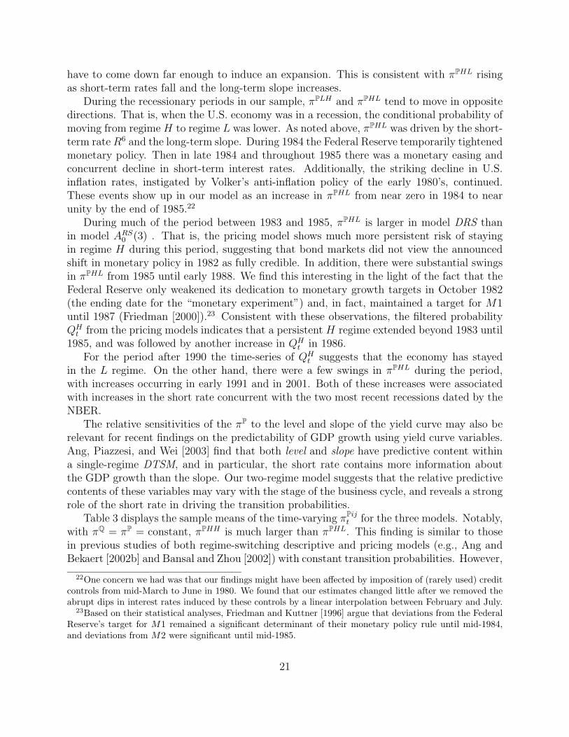
Table 3 displays the sample means of the time-varying πPijt for the three models. Notably,

with πQ = πP = constant, πPHH is much larger than πPHL. This finding is similar to thosein previous studies of both regime-switching descriptive and pricing models (e.g., Ang andBekaert [2002b] and Bansal and Zhou [2002]) with constant transition probabilities. However,

22One concern we had was that our findings might have been affected by imposition of (rarely used) creditcontrols from mid-March to June in 1980. We found that our estimates changed little after we removed theabrupt dips in interest rates induced by these controls by a linear interpolation between February and July.

23Based on their statistical analyses, Friedman and Kuttner [1996] argue that deviations from the FederalReserve’s target for M1 remained a significant determinant of their monetary policy rule until mid-1984,and deviations from M2 were significant until mid-1985.

21

Model πP xP Q

ARS0 (3)

[

87.58% 12.42%31.96% 68.04%

] [

72.00%28.00%

] [

71.91%28.09%

]

DRS

[

91.38% 8.62%46.88% 53.52%

] [

84.36%15.64%

] [

83.30%16.70%

]

ARS0 (3)[πQ = πP]

[

97.72% 2.28%5.52% 94.48%

] [

70.75%29.25%

] [

71.92%28.08%

]

Table 3: Sample means of the transition probabilities πP, the stable probability distributionxP implied by the mean transition matrices, and the sample means of the fitted probabilities(QL

t , QHt ). For model ARS

0 (3) and the descriptive model DRS the transition probabilities aretime-varying (state-dependent), while for model ARS

0 (3)[πQ = πP], are constant.

our model with time-varying regime-switching probabilities (ARS0 (3)) for U.S. treasury data

gives a smaller difference between πPHHt and πPHL

t on average, and suggests that regime Hwas notably less persistent on average than regime L. If we view regime H as capturingperiods of downturns and regime L as periods of expansions, consistent with our previousdiscussion of NBER business cycles and the probability QH

t , then this finding can be viewedas a manifestation of the well documented asymmetry in U.S. business cycles: recoveriestend to take longer than contractions (see, e.g., Neftci [1984] and Hamilton [1989]). ModelARS

0 (3) with priced, state-dependent regime shift risk captures this asymmetry, but modelARS

0 (3)[πQ = πP] with constant regime-shift probabilities does not.24

Table 3 also reveals a close match between xP, the stable probabilities implied by themean transition matrix25 and Q, the sample means of the fitted probabilities (QL

t , QHt ). In-

terestingly, both pricing models generate very similar xP and Q, although the mean transitionmatrices are dramatically different. In particular, both πPLL and πPHH are higher in modelARS

0 (3)[πQ = πP] than in model ARS0 (3). Hence, models with constant transition probabilities

not only overstate the persistence of the H regime, but also exaggerate the persistence ofthe L regime in order to match the historical distribution of “residence” in the two regimes.

The estimated risk-neutral transition probabilities from model ARS0 (3) (shown in Table

2) imply an invariant distribution of xQ = [51.50% 48.50%]′. Comparing the stable prob-abilities xQ and xP, it is seen that the economy spends much more time in regime H andmuch less time in regime L under Q than under P. This is intuitive since, with risk-aversebond investors, risk-neutral pricing will recover market prices for bonds only if we treat the

24We also confirm πPHH ≫ πPHL in the model with constant transition probabilities but priced regimeshifts (row 2 in Table 1).

25For a constant transition matrix Π, the stable (stationary, invariant) distribution x is defined by theequation Π′x = x. Equivalently, x is the limit of Π

′nx, as n → ∞. Finite-state Markov chains for which allof the elements of the transition matrix are positive are positive recurrent and irreducible, and have uniqueinvariant distributions.

22

“bad” H regime as being more likely to occur than in actuality. The diagonal elements ofπQ are statistically different from the means of the corresponding elements in πP.

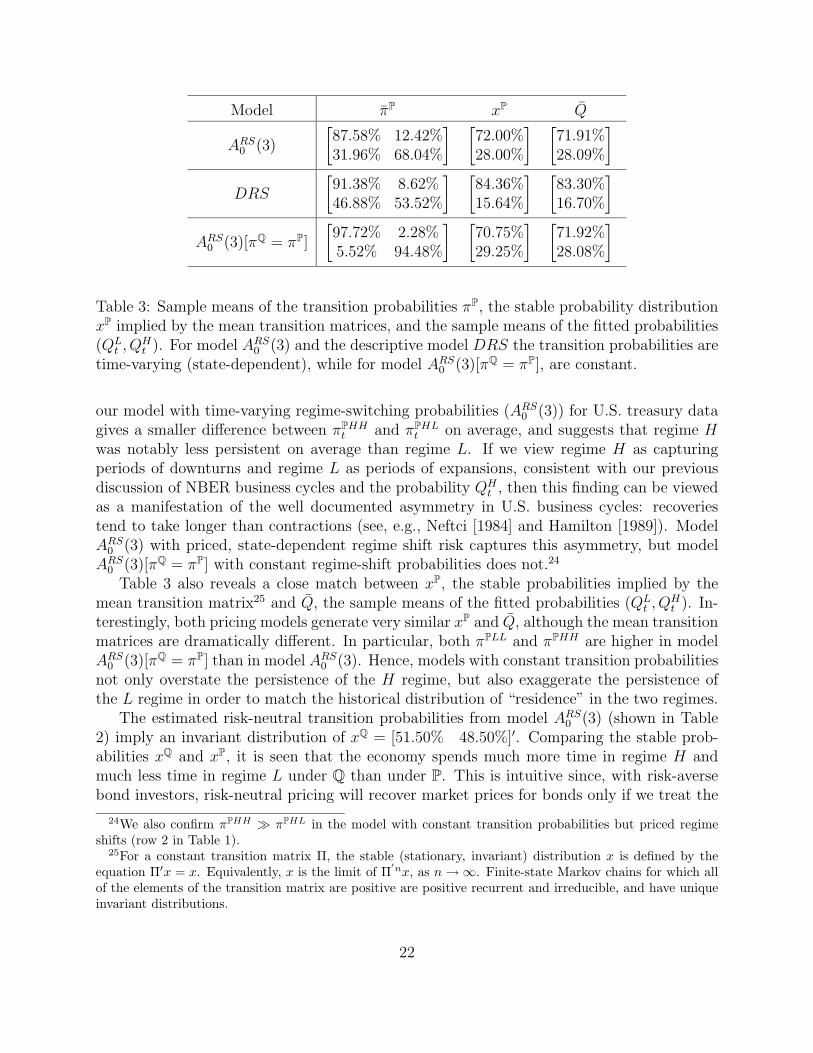
4.2 Model-Implied Means and Volatilities of Bond Yields

Figure 5 compares the sample and the model-implied means of the Treasury yields andstandard deviations (volatilities) of the monthly yield changes. To obtain the model-impliedmeans and volatilities, we treated the ML estimates as the true population parameters andsimulated 1000 time series of yields, each with the same length as that of our historical data(384 months). Then, conditional on either the L or H regime, we computed the mean of theyields and the volatility of the monthly yield changes for each simulated series, and plottedthe average and two standard deviation bands for these 1000 means and volatilities.

To construct a sample counterpart, we compute the smoothed probabilities qjt given by

(32), and then classify a date as being in regime L if qLt ≥ 0.5 or in regime H if qH

t > 0.5.After sorting the dates, we compute the sample means and volatilities of the yields in eachregime. These are reported as Sample in the plots. Figure 5 suggests that the model does avery good job at matching the first and second unconditional moments in the data, as thesample curves fall well within the two standard deviation bands of the simulated curves. Themean yield curves are upward sloping in both regimes, with the yields being notably higherin regime H.

Of particular note are the shapes of the volatility curves in the two regimes. It iswell known that in many U.S. fixed-income markets (e.g., Treasury bond, swaps, etc.),the term structures of unconditional yield volatilities are hump-shaped (see, e.g., Litterman,Scheinkman, and Weiss [1991]), with the peak of the hump being approximately at two yearsto maturity.26 Under our classification of dates into regimes, the hump in volatility is anL-regime phenomenon. Fleming and Remolona [1999] present evidence linking the hump tomarket reactions to macroeconomic announcements. Through the lens of our model, it ap-pears that these, and possibly other, sources of yield volatility show up as a hump in volatilityprimarily during relatively tranquil, expansionary phases of the business cycle. When theeconomy is in regime H, volatility is high and the risk factors mean-revert to their long-runmeans relatively quickly (κPH in Table 2). The fast mean reversion in regime H swamps ahumped reaction (if any) to macroeconomic news, and induces the steeply downward slopingterm structure of (unconditional) volatility.

Pursuing the latter point, it is the interaction between the factor correlations and theirrates of mean reversion that largely induce humped-shaped term structures of volatility indynamic term structure models (Dai and Singleton [2000]). Indeed, when we estimateda restricted version of model ARS

0 (3) with diagonal κPj, Σj, and λjY matrices, simulations

confirmed that mean reversion induces downward sloping term structures of volatility in boththe H and L regimes. This is why we highlight the flexibility associated with correlated

26Figure 5 also shows the “snake” shaped pattern in historical yield volatilities for very short-term bonds.This pattern is partially captured by our three-factor model. The findings in both Longstaff, Santa-Clara,and Schwartz [2001] and Piazzesi [2005] suggest that the addition of a fourth factor would allow our modelto replicate this pattern even better.

23

0 5 102

4

6

8

Maturity (Year)

Mea

n in

Reg

ime

L (%

)

SampleSimu

0 5 106

8

10

12

14

Maturity (Year)

Mea

n in

Reg

ime

H (

%)

SampleSimu

0 5 100.25

0.3

0.35

Maturity (Year)

Vol

atili

ty in

Reg

ime

L (%

)

SampleSimu

0 5 100

0.5

1

1.5

Maturity (Year)V

olat

ility

in R

egim

e H

(%

)

SampleSimu

Figure 5: Term structures of unconditional means of Treasury bond yields and volatilitiesof monthly yield changes implied by model ARS

0 (3). The solid lines show the sample results,obtained by computing sample means and volatilities after allocating dates to regimes basedon the smoothed probabilities qj

t . The dotted lines and the crosses plot the averages and twostandard deviations for the means and volatilities computed from the time series of yieldssimulated from the model. Both means and volatilities are annualized.

factors in Gaussian affine models relative to multi-factor CIR models with independentfactors. Ang and Bekaert [2005] also constrain the “level” and “slope” (latent) factors intheir regime-switching Gaussian models to be mutually independent within all regimes.

In unreported results, we also confirm that the simulated curves from model ARS0 (3)[πQ =

πP], in which regime-shift risk is not priced and regime-switching probabilities are state-independent, perform similarly well in matching the sample mean and volatility curves.By and large, there is not a large difference between the model-implied first and secondunconditional moments across these two models.

We examine the model-implied conditional volatilities in Section 6 as part of our assess-ment of the robustness of the properties of model ARS

0 (3) to the presence of within-regimetime-varying volatility.

5 Excess Returns and Market Prices of Risk

In this section we return to one of the primary motivations for our analysis, namely, aninvestigation of the contributions of factor and regime-shift risk premiums to the temporal

24

variation in expected excess returns.We start by presenting the decomposition of expected excess returns into components

associated with regime-shift and factor risks. Let pjt,n ≡ log Dj

t,n denote the log price of an-period bond at time t and in regime st = j. The one-period expected excess return on then-period bond is (see appendix A for more details)

Et[pt+1,n−1|st = j] − pjt,n + pj

t,1 = ρRSjt,n + ρFj

t,n, (36)

where

ρRSjt,n = log

e∑S

k=0π

Pjkt (−Ak

n−1)

∑S

k=0 πQjke−Akn−1

, (37)

ρFjt,n = −1

2B′

n−1ΣjΣj′Bn−1 − B′

n−1ΣjΛj

t . (38)

Since econometricians do not observe the regimes, we evaluate the expected excess returnsconditional on Jt:

Et[pt+1,n−1 − pt,n + pt,1|Jt] =∑

j

Et[pt+1,n−1 − pt,n + pt,1|st = j, Jt]Qjt

=∑

j

ρRSjt,n Qj

t +∑

j

ρFjt,nQ

jt ≡ ρRS

t,n + ρFt,n,

where the regime-specific components ρRSjt,n and ρFj

t,n are weighted by regime probabilities Qjt .

The regime-shift component ρRSjt,n is determined largely by the difference between the

historical and risk neutral transition probabilities and the regime dependence of Akn−1. This

can be seen more clearly from its linear expansion,

ρRSjt,n ≈

S∑

k=0

(πQjk − πPjkt )Ak

n−1 (39)

=

(πQLH − πPLHt )(AH

n−1 − ALn−1), if st = L,

(πQHL − πPHLt )(AL

n−1 − AHn−1), if st = H.

(40)

Though ρRSjt,n is nonzero even if πQjk = πPjk, due to the convexity effect associated with

continuously compounded returns, the quantitative importance of this convexity effect isnegligible (see below). Thus, the within-regime variation in ρRSj

t,n is determined largely by

time variation in πPjkt and, hence, the historical probabilities of a change in regime potentially

play a central role in the temporal variation in expected excess returns.The convexity effect also produces the first term in ρFj

t,n. The second term, on the other

hand, is proportional to the market price of factor risk, Λjt , and the amount of exposure to

the factor risk, B′n−1Σ

j. Substituting ΣjΛjt = λj

0 + λjY Yt into (38), we see that a constant

MPF risk (λj0 6= 0, λj

Y = 0) would only induce regime specific, constant expected returns.

25

Consequently, with λjY = 0, the only source of temporal variation in the component ρF

t,n of

expected excess returns is the variation in the Qjt . By allowing for λj

Y 6= 0 we introducewithin-regime variation in ρFj

t and, thereby, allow for much richer historical patterns in thevariation of the component ρF

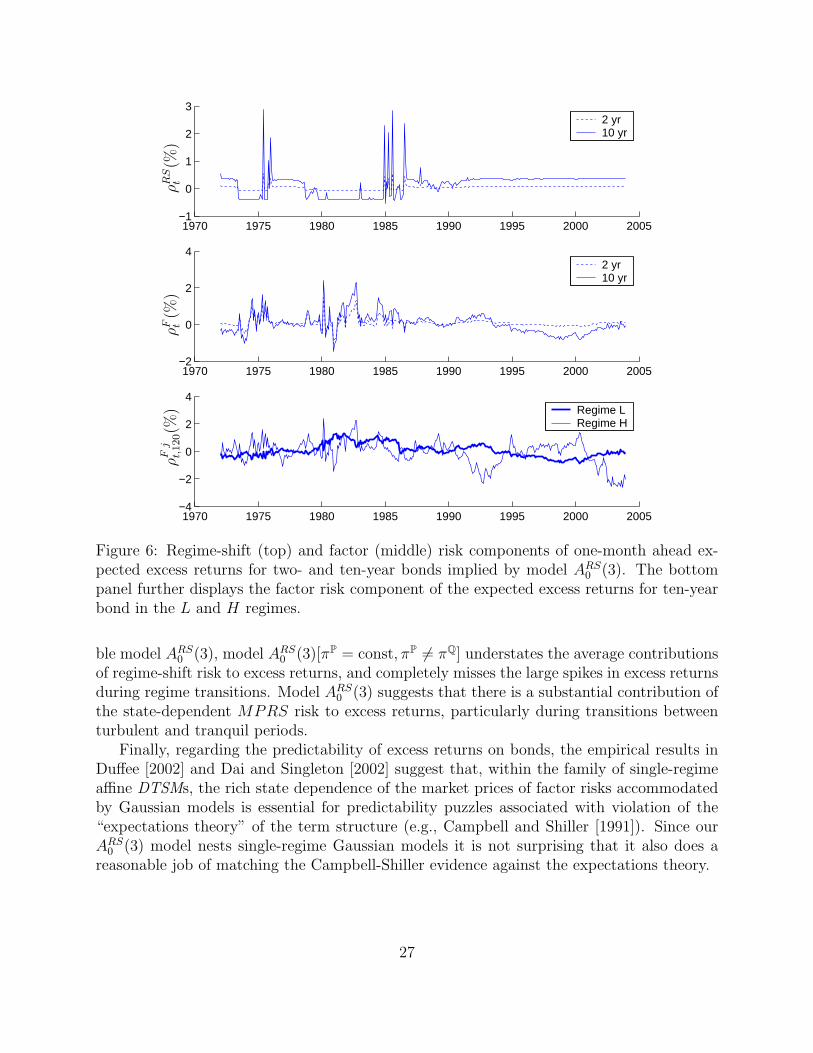
t,n.Figure 6 plots ρRS

t,n and ρFt,n for n = 24 and 120 months. During extended L (H) regimes

we observe persistent positive (negative) levels of the regime shift component of the expectedexcess returns. Intuitively, during the L regime the physical probability of switching to theH regime is extremely low (almost zero), lower than the πQLH . The bonds are priced inthe markets as if the probabilities of going into recessions are higher under the risk-neutralmeasure. This pushes down the current bond prices, yielding a positive expected returncomponent. Similarly, during the H regime, the relatively higher risk neutral probability ofswitching to the L regime pushes up the current bond prices and yields a negative expectedreturn. The magnitudes of these persistent levels of the regime-shift components are about0.2 to 0.3% (monthly) on a ten-year bond, in comparison to a 0.6% standard deviation ofthe factor risk component.

The large spikes around the mid-1970’s and mid-1980’s in the regime-shift risk componentare attributable to ρRS H

t,n , the H regime component, and thus are associated with the swingsin the πPHL during these two periods. We have noted earlier that the mid-1980’s episodesuggests investors doubted the credibility of the Federal Reserve’s announced change inmonetary policy. These spikes are completely missed in the model-implied expected returnsfor the single-regime A0(3) model (see Figure 1).

The bottom panel of Figure 6 decomposes the factor risk component into values duringthe L and H regimes based on model ARS

0 (3) (the ρFjt,n in (38)). Consistent with the view that

expected returns should not fluctuate dramatically under “normal” circumstances, the curvesare much smoother in regime L (thick line) than in regime H (thin line).27 A very differentimpression comes from inspection of the expected excess returns from the correspondingsingle-regime Gaussian A0(3) model displayed in Figure 1 (induced solely by factor risks).They look much more like the choppy patterns during regime H than the relatively smoothbehavior during regime L. This finding lends support to a basic premise of this paper;namely, omission of the regime-switching process tends to distort the model-implied (factorrisk component of) excess returns both in tranquil and turbulent times.

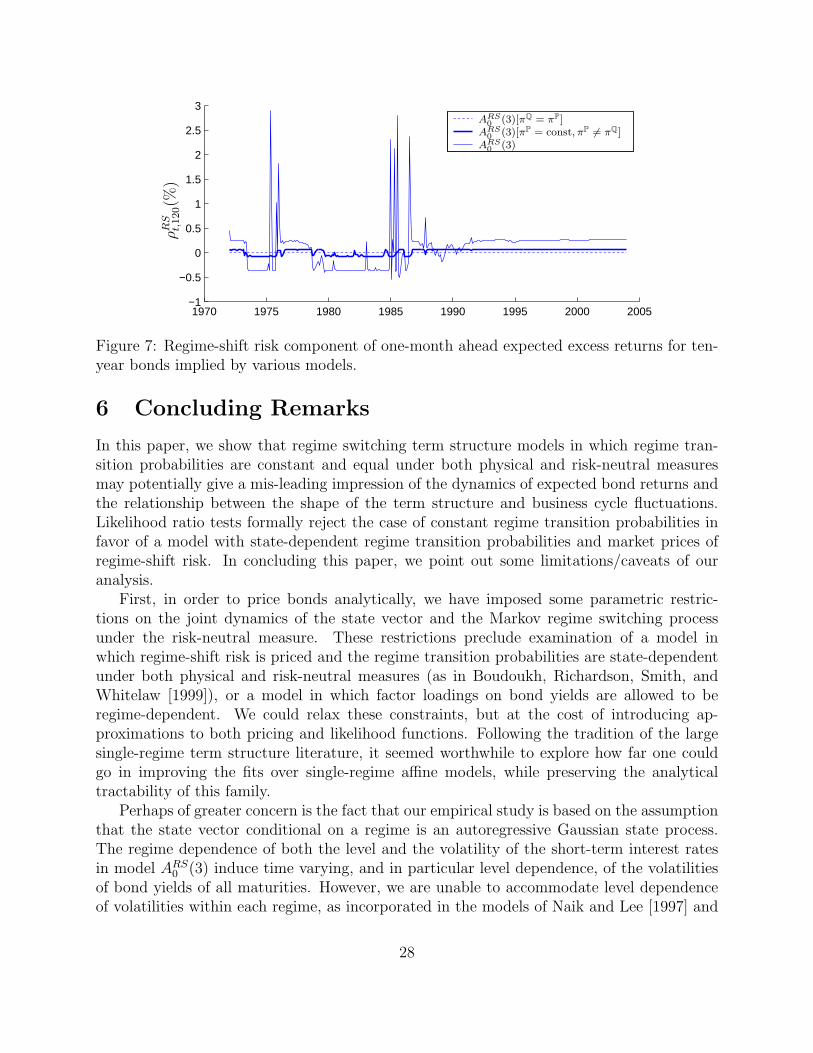
To demonstrate the critical role of state-dependent MPRS risks in capturing the vari-ations in excess returns, Figure 7 plots the regime-shift component of expected returns ona ten-year bond implied by three models, ordered from the least to the most flexible spec-ifications of the MPRS risk. Model ARS

0 (3)[πQ = πP] restricts Γjkt = 0, and the regime

-shift component of excess returns is comprised solely of the convexity term. As anticipated,the magnitudes are negligible, with maximums of about 0.003%. Allowing for a constant,nonzero Γjk

t in model ARS0 (3)[πP = const, πP 6= πQ] gives rise to persistent positive (negative)

contributions to excess returns within the L (H) regime. However, relative to our most flexi-

27The regime dependent characteristics of ρFt are attributable to the corresponding market prices of factor

risks in L and H regimes. We confirm in unreported results that the market prices of factor risks are muchsmoother in the L regime than in the H regime.

26

1970 1975 1980 1985 1990 1995 2000 2005−1

0

1

2

32 yr10 yr

1970 1975 1980 1985 1990 1995 2000 2005−2

0

2

42 yr10 yr

1970 1975 1980 1985 1990 1995 2000 2005−4

−2

0

2

4Regime LRegime H

ρR

St

(%)

ρF t(%

)ρ

Fj

t,120(%

)

Figure 6: Regime-shift (top) and factor (middle) risk components of one-month ahead ex-pected excess returns for two- and ten-year bonds implied by model ARS

0 (3). The bottompanel further displays the factor risk component of the expected excess returns for ten-yearbond in the L and H regimes.

ble model ARS0 (3), model ARS

0 (3)[πP = const, πP 6= πQ] understates the average contributionsof regime-shift risk to excess returns, and completely misses the large spikes in excess returnsduring regime transitions. Model ARS

0 (3) suggests that there is a substantial contribution ofthe state-dependent MPRS risk to excess returns, particularly during transitions betweenturbulent and tranquil periods.

Finally, regarding the predictability of excess returns on bonds, the empirical results inDuffee [2002] and Dai and Singleton [2002] suggest that, within the family of single-regimeaffine DTSMs, the rich state dependence of the market prices of factor risks accommodatedby Gaussian models is essential for predictability puzzles associated with violation of the“expectations theory” of the term structure (e.g., Campbell and Shiller [1991]). Since ourARS

0 (3) model nests single-regime Gaussian models it is not surprising that it also does areasonable job of matching the Campbell-Shiller evidence against the expectations theory.

27

1970 1975 1980 1985 1990 1995 2000 2005−1

−0.5

0

0.5

1

1.5

2

2.5

3

ρR

St,120(%

)

ARS0

(3)ARS

0(3)[πP = const, πP 6= πQ]

ARS0

(3)[πQ = πP]

Figure 7: Regime-shift risk component of one-month ahead expected excess returns for ten-year bonds implied by various models.

6 Concluding Remarks

In this paper, we show that regime switching term structure models in which regime tran-sition probabilities are constant and equal under both physical and risk-neutral measuresmay potentially give a mis-leading impression of the dynamics of expected bond returns andthe relationship between the shape of the term structure and business cycle fluctuations.Likelihood ratio tests formally reject the case of constant regime transition probabilities infavor of a model with state-dependent regime transition probabilities and market prices ofregime-shift risk. In concluding this paper, we point out some limitations/caveats of ouranalysis.

First, in order to price bonds analytically, we have imposed some parametric restric-tions on the joint dynamics of the state vector and the Markov regime switching processunder the risk-neutral measure. These restrictions preclude examination of a model inwhich regime-shift risk is priced and the regime transition probabilities are state-dependentunder both physical and risk-neutral measures (as in Boudoukh, Richardson, Smith, andWhitelaw [1999]), or a model in which factor loadings on bond yields are allowed to beregime-dependent. We could relax these constraints, but at the cost of introducing ap-proximations to both pricing and likelihood functions. Following the tradition of the largesingle-regime term structure literature, it seemed worthwhile to explore how far one couldgo in improving the fits over single-regime affine models, while preserving the analyticaltractability of this family.

Perhaps of greater concern is the fact that our empirical study is based on the assumptionthat the state vector conditional on a regime is an autoregressive Gaussian state process.The regime dependence of both the level and the volatility of the short-term interest ratesin model ARS

0 (3) induce time varying, and in particular level dependence, of the volatilitiesof bond yields of all maturities. However, we are unable to accommodate level dependenceof volatilities within each regime, as incorporated in the models of Naik and Lee [1997] and

28

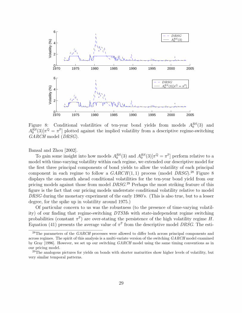
1970 1975 1980 1985 1990 1995 2000 20050

2

4

6

Vol

atili

ty (

%)

1970 1975 1980 1985 1990 1995 2000 20050

2

4

6

Vol

atili

ty (

%)

DRSG

DRSG

ARS0

(3)

ARS0

(3)[πQ = πP]

Figure 8: Conditional volatilities of ten-year bond yields from models ARS0 (3) and

ARS0 (3)[πQ = πP] plotted against the implied volatility from a descriptive regime-switching

GARCH model (DRSG).

Bansal and Zhou [2002].To gain some insight into how models ARS

0 (3) and ARS0 (3)[πQ = πP] perform relative to a

model with time-varying volatility within each regime, we extended our descriptive model forthe first three principal components of bond yields to allow the volatility of each principalcomponent in each regime to follow a GARCH(1, 1) process (model DRSG).28 Figure 8displays the one-month ahead conditional volatilities for the ten-year bond yield from ourpricing models against those from model DRSG.29 Perhaps the most striking feature of thisfigure is the fact that our pricing models understate conditional volatility relative to modelDRSG during the monetary experiment of the early 1980’s. (This is also true, but to a lesserdegree, for the spike up in volatility around 1975.)

Of particular concern to us was the robustness (to the presence of time-varying volatil-ity) of our finding that regime-switching DTSMs with state-independent regime switchingprobabilities (constant πP) are over-stating the persistence of the high volatility regime H.Equation (41) presents the average value of πP from the descriptive model DRSG. The esti-

28The parameters of the GARCH processes were allowed to differ both across principal components andacross regimes. The spirit of this analysis is a multi-variate version of the switching GARCH model examinedby Gray [1996]. However, we set up our switching GARCH model using the same timing conventions as inour pricing model.

29The analogous pictures for yields on bonds with shorter maturities show higher levels of volatility, butvery similar temporal patterns.

29

mates are very similar to those from the model DRS:

πDRSG =

[

91.39% 8.61%49.11% 50.89%

]

. (41)

This extended descriptive analysis with model DRSG does not, of course, allow us to assessthe implications of within-regime time-varying volatility for the structure of the marketprices of factor or regime-shift risks. Such an assessment would require a regime-shiftingDTSM that allows for both within regime stochastic volatility and state-dependent regime-shift probabilities. Nevertheless, given the similarity between the results for models DRSand DRSG, we are reassured that some of our key findings– in particular, the asymmetry inthe persistence of regimes– are robust to extended specifications of volatility beyond whatis inherent in model ARS

0 (3).Finally, a natural question is whether our findings are sensitive to our choice of sample

period. The nature of a regime-switching model is such that the answer has to be (a qualified)yes. As documented above, in both our pricing and descriptive regime-switching models, theregimes identified by our model are related to stages of the business cycle. For such anidentification to be feasible, it is essential that the sample period span a sufficient number ofcycles. Otherwise, the flexibility of a regime-switching model will largely be used to capturerelatively minor within-cycle variations in the conditional distributions of bond yields.

This was confirmed upon re-estimation of model ARS0 (3) over the post-1987 sample. For

this shorter sample, the two-regime model associated the period 1987–1992 with the Hregime, and the post-1992 with the L regime. The pre-1992 H regime spans the recessionof the early 1990’s. Not unexpectedly, the differences in the volatilities of the factors acrossthe H and L regimes are much smaller than those obtained for the full sample period(the diagonal elements of

√12ΣH are (0.96, 1.06, 1.26) in the shortened sample compared to

(1.51, 2.03, 4.56) in the full sample). This is consistent with the full-sample results, whichtreat the post-1987 era as a homogeneous L regime. Many other features of the full-sampleresults, including faster rates of mean reversion in the H regime and asymmetry in thematrix πP when these probabilities are state-dependent, remain qualitatively the same inthe post-1987 period. These findings provide further assurance that our key results arerobust.

30

A Decomposition of Expected Excess Returns

The price of a n-period bond is

Djt,n = e−A

jn−B′

nYt .

The log price is

pjt,n ≡ log Dj

t,n = log EQt

[

e−rjt Dt+1,n−1|st = j

]

= −rjt + log

(

S∑

k=0

πQjkEQt

[

Dkt+1,n−1|st = j

]

)

= −rjt + log

(

S∑

k=0

πQjke−Akn−1EQ

t

[

e−B′

n−1Yt+1|st = j

]

)

= −rjt + log

(

S∑

k=0

πQjke−Akn−1

)

− B′n−1µ

Qjt +

1

2B′

n−1ΣjΣj′Bn−1.

The expected value of the log price is

Et[pt+1,n|st = j]

=S

∑

k=0

πPjkt Et[p

kt+1,n|st = j]

=S

∑

k=0

πPjkt

(

−Akn − B′

nEt[Yt+1|st = j])

= −(

S∑

k=0

πPjkt Ak

n

)

− B′nµ

Pjt .

The expected excess return is then

Et[pt+1,n−1|st = j] − pjt,n + pj

t,1

= −(

S∑

k=0

πPjkt Ak

n−1

)

− B′n−1µ

Pjt

+rjt − log

(

S∑

k=0

πQjke−Akn−1

)

+ B′n−1µ

Qjt − 1

2B′

n−1ΣjΣj′Bn−1

−rjt

= loge

∑Sk=0

πPjkt (−Ak

n−1)

∑S

k=0 πQjke−Akn−1

− 1

2B′

n−1ΣjΣj′Bn−1 − B′

n−1ΣjΛj

t .

31

References

Ait-Sahalia, Y. (1996). Testing Continuous-Time Models of the Spot Interest Rate. Reviewof Financial Studies 9 (2), 385 – 426.

Ang, A. and G. Bekaert (2002a). Regime Switches in Interest Rates. Journal of Businessand Economic Statistics 20, 163–182.

Ang, A. and G. Bekaert (2002b). Short Rate Nonlinearities and Regime Switches. Journalof Economic Dynamics and Control 26, 1243–1274.

Ang, A. and G. Bekaert (2005). The Term Structure of Real Rates and Expected Inflation.Working paper, Columbia University.

Ang, A. and M. Piazzesi (2003). A No-Arbitrage Vector Autoregression of Term Struc-ture Dynamics with Macroeconomic and Latent Variables. Journal of Monetary Eco-nomics 50, 745–787.

Ang, A., M. Piazzesi, and M. Wei (2003). What Does the Yield Curve Tell us About GDPGrowth? Working Paper, Columbia University.

Bansal, R. and H. Zhou (2002). Term Structure of Interest Rates with Regime Shifts.Journal of Finance 57, 1997 – 2043.

Bekaert, G. and S. Grenadier (2001). Stock and Bond Pricing in an Affine Equilibrium.Working Paper, Stanford University.

Bliss, R. R. (1997). Testing Term Structure Estimation Methods. Advances in Futures andOptions Research 9, 197–231.

Boudoukh, J., M. Richardson, T. Smith, and R. F. Whitelaw (1999). Regime Shifts andBond Returns. Working paper, New York University.

Campbell, J. and R. Shiller (1991). Yield Spreads and Interest Rate Movements: A Bird’sEye View. Review of Economic Studies 58, 495–514.

Cecchetti, S., P. Lam, and N. Mark (1993). The Equity Premium and the Risk-free Rate:Matching the Moments. Journal of Monetary Economics 31, 21–45.

Chapman, D. and N. Pearson (2000). Is the Short-Rate Drift Actually Nonlinear? Journalof Finance 55, 355–388.

Chen, R. and L. Scott (1995). Interest Rate Options in Multifactor Cox-Ingersoll-RossModels of the Term Structure. Journal of Fixed Income Winter, 53–72.

Dai, Q. and K. Singleton (2000). Specification Analysis of Affine Term Structure Models.Journal of Finance 55, 1943–1978.

Dai, Q. and K. Singleton (2002). Expectations Puzzles, Time-Varying Risk Premia, andAffine Models of the Term Structure. Journal of Financial Economics 63, 415–441.

Dai, Q. and K. Singleton (2003). Term Structure Dynamics in Theory and Reality. Reviewof Financial Studies 16, 631–678.

32

Duarte, J. (2004). Evaluating an Alternative Risk Preference in Affine Term StructureModels. Review of Financial Studies 17, 379–404.

Duffee, G. R. (2002). Term Premia and Interest Rate Forecasts in Affine Models. Journalof Finance 57, 405–443.

Duffie, D. and K. Singleton (1997). An Econometric Model of the Term Structure ofInterest Rate Swap Yields. Journal of Finance 52, 1287–1321.

Fama, E. F. and R. R. Bliss (1987). The Information in Long-Maturity Forward Rates.American Economic Review 77 (4), 680–692.

Fisher, M., D. Nychka, and D. Zervos (1995). Fitting the Term Structure of Interest Rateswith Smoothing Splines. Working Paper 95-1, Finance and Economics Discussion SeriesFederal Reserve Board.

Fleming, M. J. and E. Remolona (1999). The Term Structure of Announcement Effects.FRB New York Staff Report No. 76.

Friedman, B. (2000). The Role of Interest Rates in Federal Reserve Policy Making. NBERWorking Paper 8047.

Friedman, B. and K. Kuttner (1996). A Price Target for U.S. Monetary Policy? Lessonsfrom the Experience with Monetary Growth Targets. Brookings Papers on EconomicActivity 1, 77–146.

Garcia, R. and P. Perron (1996). An Analysis of the Real Interest Rate Under RegimeShifts. Review of Economics and Statistics , 111–125.

Gourieroux, C., A. Monfort, and V. Polimenis (2002). Affine Term Structure Models.Working paper, University of Toronto, Canada.

Gray, S. (1996). Modeling the Conditional Distribution of Interest Rates as a RegimeSwitching Process. Journal of Financial Economics 42, 27–62.

Hamilton, J. (1989). A New Approach to the Economic Analysis of Nonstationary TimeSeries and the Business Cycle. Econometrica 57, 357–384.

Landen, C. (2000). Bond Pricing in a Hidden Markov Model of the Short Rate. Financeand Stochastics 4, 371–389.

Litterman, R., J. Scheinkman, and L. Weiss (1991). Volatility and the Yield Curve. Journalof Fixed Income 1, 49–53.

Liu, J., F. Longstaff, and J. Pan (2002). Dynamic Asset Allocation with Event Risk.forthcoming, Journal of Finance.

Longstaff, F., P. Santa-Clara, and E. Schwartz (2001). The Relative Valuation of Capsand Swaptions: Theory and Empirical Evidence. Journal of Finance 56, 2067–2109.

McCulloch, J. (1975). The Tax-Adjusted Yield Curve. Journal of Finance 30, 811–830.

Naik, V. and M. H. Lee (1997). Yield Curve Dynamics with Discrete Shifts in EconomicRegimes: Theory and Estimation. Working paper, Faculty of Commerce, University ofBritish Columbia.

33

Neftci, S. (1984). Are Economic Time Series Asymmetric Over the Business Cycle? Jour-nal of Political Economy 92, 307–328.

Nelson, C. and A. Siegel (1987). Parsimonious Modelling of Yield Curves. Journal ofBusiness 60, 473–489.

Pan, J. (2002). The Jump-Risk Premia Implicit in Options: Evidence from an IntegratedTime-Series Study. Journal of Financial Economics 63, 3–50.

Pearson, N. D. and T. Sun (1994). Exploiting the Conditional Density in Estimating theTerm Structure: An Application to the Cox, Ingersoll, and Ross Model. Journal ofFinance 49, 1279–1304.

Piazzesi, M. (2005). Bond Yields and the Federal Reserve. Journal of Political Econ-omy 113, 311–344.

Stanton, R. (1997). A Nonparametric Model of Term Structure Dynamics and the MarketPrice of Interest Rate Risk. Journal of Finance 52, 1973–2002.

Veronesi, P. and F. Yared (2000). Short and Long Horizon Term and Inflation Risk Premiain the U.S. Term Structure: Evidence from an Integrated Model for Nominal and RealBond Prices under Regime Shifts. Working Paper, University of Chicago.

Waggoner, D. (1997). Spline Methods for Extracting Interest Rate Curves from CouponBond Prices. Working Paper, Federal Reserve Bank Atlanta.

Wu, S. and Y. Zeng (2003). A General Equilibrium Model of the Term Structure of InterestRates under Regime-switching Risk. Working Paper, University of Kansas.

34