Regularity Estimates in Maximum Norm forElliptic and Parabolic Finite Difference Equations

J. Thomas BealeDuke University

www.math.duke.edu/faculty/beale

Discrete versions of ellliptic or parabolic equationsfinite differences on gridsestimates in maximum norm

Inverting discrete Laplacian gains two differences, almost?L2 estimates are standard, fine with enough smoothnessFor limited smoothness, e.g. with interfaces,

largest error typically on a small setL∞ is a more meaningful measure of error than L2

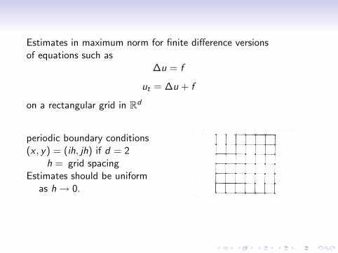
Estimates in maximum norm for finite difference versionsof equations such as

∆u = f

ut = ∆u + f

on a rectangular grid in Rd

periodic boundary conditions(x , y) = (ih, jh) if d = 2

h = grid spacingEstimates should be uniform

as h→ 0.

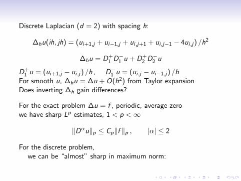
Discrete Laplacian (d = 2) with spacing h:

∆hu(ih, jh) = (ui+1,j + ui−1,j + ui ,j+1 + ui ,j−1 − 4ui ,j) /h2

∆hu = D+1 D−1 u + D+

2 D−2 u

D+1 u = (ui+1,j − ui ,j) /h , D−1 u = (ui ,j − ui−1,j) /h

For smooth u, ∆hu = ∆u + O(h2) from Taylor expansionDoes inverting ∆h gain differences?

For the exact problem ∆u = f , periodic, average zerowe have sharp Lp estimates, 1 < p <∞

‖Dαu‖p ≤ Cp‖f ‖p , |α| ≤ 2

For the discrete problem,we can be “almost” sharp in maximum norm:

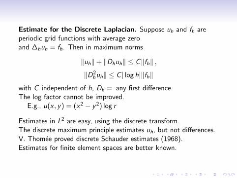
Estimate for the Discrete Laplacian. Suppose uh and fh areperiodic grid functions with average zeroand ∆huh = fh. Then in maximum norms

‖uh‖+ ‖Dhuh‖ ≤ C‖fh‖ ,

‖D2huh‖ ≤ C | log h|‖fh‖

with C independent of h, Dh = any first difference.The log factor cannot be improved.

E.g., u(x , y) = (x2 − y2) log r

Estimates in L2 are easy, using the discrete transform.The discrete maximum principle estimates uh, but not differences.V. Thomee proved discrete Schauder estimates (1968).Estimates for finite element spaces are better known.

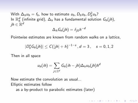
With ∆huh = fh, how to estimate uh,Dhuh,D2huh?

In Rdh (infinite grid), ∆h has a fundamental solution Gh(jh),

jh ∈ Rd

∆hGh(jh) = δj0h−d

Pointwise estimates are known from random walks on a lattice,

|DshGh(jh)| ≤ C (|jh|+ h)−1−s , d = 3 , s = 0, 1, 2

Then in all space

uh(ih) =∑j∈Zd

Gh(ih − jh)∆huh(jh)hd

Now estimate the convolution as usual...Elliptic estimates follow

as a by-product to parabolic estimates (later)

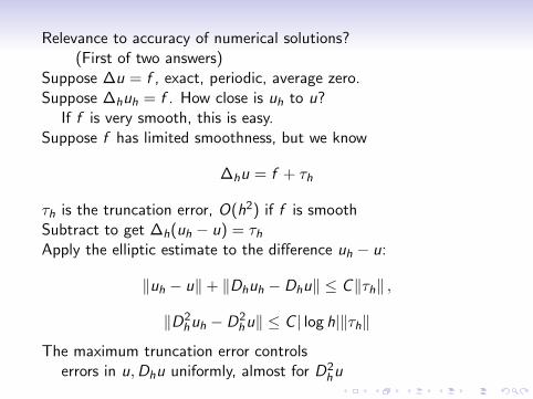
Relevance to accuracy of numerical solutions?(First of two answers)

Suppose ∆u = f , exact, periodic, average zero.Suppose ∆huh = f . How close is uh to u?

If f is very smooth, this is easy.Suppose f has limited smoothness, but we know

∆hu = f + τh

τh is the truncation error, O(h2) if f is smoothSubtract to get ∆h(uh − u) = τhApply the elliptic estimate to the difference uh − u:

‖uh − u‖+ ‖Dhuh − Dhu‖ ≤ C‖τh‖ ,

‖D2huh − D2

hu‖ ≤ C | log h|‖τh‖

The maximum truncation error controlserrors in u,Dhu uniformly, almost for D2

hu

Poisson problem with an interface

∆u− = f− in Ω− , ∆u+ = f+ in Ω+ ,

[u] = g0 on Γ , [∂nu] = g1 on Γ

−

+

ΩΩ Γ

∆hu(ih)−∆u(ih) = O(h2)at regular points,away from Γ

∆hu(ih)−∆u(ih) is largeat irregular points,where ∆h crosses Γ

If we improve the truncation error to O(h)at the irregular points, then

the error in u is uniformly O(h2), andthe error in Dhu is uniformly O(h2| log h|)

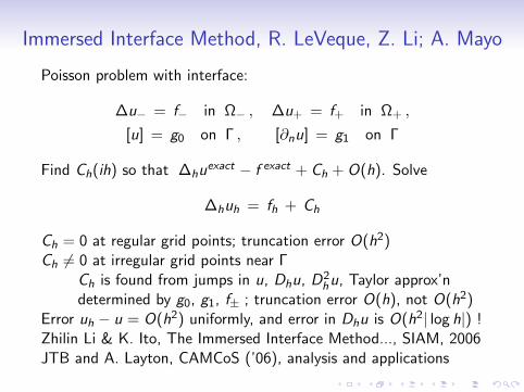
Immersed Interface Method, R. LeVeque, Z. Li; A. Mayo

Poisson problem with interface:

∆u− = f− in Ω− , ∆u+ = f+ in Ω+ ,

[u] = g0 on Γ , [∂nu] = g1 on Γ

Find Ch(ih) so that ∆huexact − f exact + Ch + O(h). Solve

∆huh = fh + Ch

Ch = 0 at regular grid points; truncation error O(h2)Ch 6= 0 at irregular grid points near Γ

Ch is found from jumps in u, Dhu, D2hu, Taylor approx’n

determined by g0, g1, f± ; truncation error O(h), not O(h2)Error uh − u = O(h2) uniformly, and error in Dhu is O(h2| log h|) !Zhilin Li & K. Ito, The Immersed Interface Method..., SIAM, 2006JTB and A. Layton, CAMCoS (’06), analysis and applications

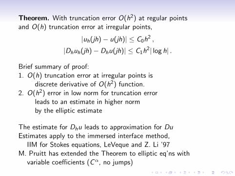
Theorem. With truncation error O(h2) at regular pointsand O(h) truncation error at irregular points,

|uh(jh)− u(jh)| ≤ C0h2 ,

|Dhuh(jh)− Dhu(jh)| ≤ C1h2| log h| .

Brief summary of proof:1. O(h) truncation error at irregular points is

discrete derivative of O(h2) function.2. O(h2) error in low norm for truncation error

leads to an estimate in higher normby the elliptic estimate

The estimate for Dhu leads to approximation for DuEstimates apply to the immersed interface method,

IIM for Stokes equations, LeVeque and Z. Li ’97M. Pruitt has extended the Theorem to elliptic eq’ns with

variable coefficients (Cα, no jumps)

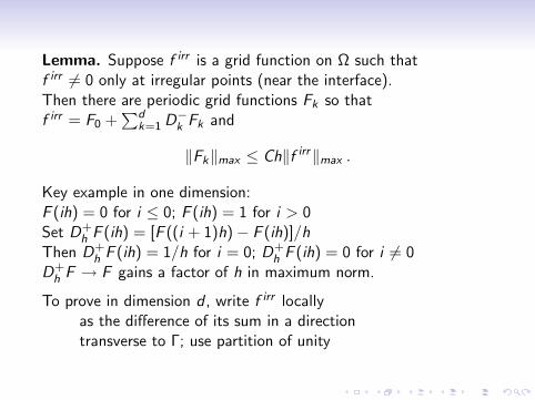
Lemma. Suppose f irr is a grid function on Ω such thatf irr 6= 0 only at irregular points (near the interface).Then there are periodic grid functions Fk so thatf irr = F0 +

∑dk=1 D−k Fk and

‖Fk‖max ≤ Ch‖f irr‖max .

Key example in one dimension:F (ih) = 0 for i ≤ 0; F (ih) = 1 for i > 0Set D+

h F (ih) = [F ((i + 1)h)− F (ih)]/hThen D+

h F (ih) = 1/h for i = 0; D+h F (ih) = 0 for i 6= 0

D+h F → F gains a factor of h in maximum norm.

To prove in dimension d , write f irr locallyas the difference of its sum in a directiontransverse to Γ; use partition of unity

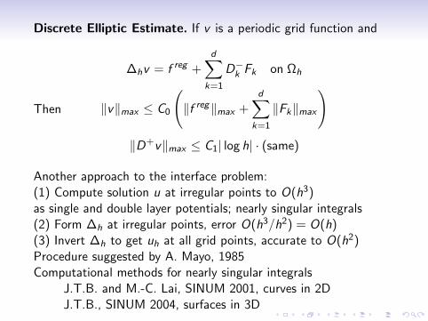
Discrete Elliptic Estimate. If v is a periodic grid function and

∆hv = f reg +d∑

k=1

D−k Fk on Ωh

Then ‖v‖max ≤ C0

(‖f reg‖max +

d∑k=1

‖Fk‖max

)‖D+v‖max ≤ C1| log h| · (same)

Another approach to the interface problem:(1) Compute solution u at irregular points to O(h3)as single and double layer potentials; nearly singular integrals(2) Form ∆h at irregular points, error O(h3/h2) = O(h)(3) Invert ∆h to get uh at all grid points, accurate to O(h2)Procedure suggested by A. Mayo, 1985Computational methods for nearly singular integrals

J.T.B. and M.-C. Lai, SINUM 2001, curves in 2DJ.T.B., SINUM 2004, surfaces in 3D

Gain in Regularity for Parabolic Difference Equations

Estimates for discrete versions of

ut = ∆u , u(·, 0) = u0

Use grid in space with x = jh, j ∈ Zd

Discretize ∆ with ∆h as beforeWe should get estimates for Dhu and D2

huTime t = nk, time step k ; how to discretize in time?Simplest version, “forward Euler”: un+1 − un = k∆hu

n

This (explicit) method requires k = ch2

Implicit methods are better, allow k = chThe simplest implicit method is “backward Euler”

un+1 − un = k∆hun+1 or un+1 = (I − k∆h)−1un

Then un = (I − k∆h)−nu0 = s(k∆h)nu0 , s(z) ≡ 1/(1− z)Backward Euler has regularity but first order error O(k)There are “good” second order methods, error O(k2)

Gain in Regularity for Parabolic Difference Equations

Suppose we approximate (using backward Euler)

ut = ∆u + f , u(·, 0) = 0

by un+1 − un = k∆hun+1 + kf n+1

or un+1 = (I − k∆h)−1(un + kf n+1

)Then

‖un‖+ ‖Dhun‖ ≤ C1 sup

t≤T‖f (·, t)‖

‖D2hun‖ ≤ C2 (1 + | log h|) sup

t≤T‖f (·, t)‖

Similar statements hold for a class of time-stepping methods...Interpretation: ucomputed − uexact and differences

are bounded by maximum truncation error.J.T.B. “Smoothing properties...”, SINUM 2009.

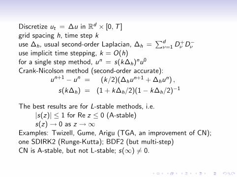
Discretize ut = ∆u in Rd × [0,T ]grid spacing h, time step kuse ∆h, usual second-order Laplacian, ∆h =

∑dν=1 D+

ν D−νuse implicit time stepping, k = O(h)for a single step method, un = s(k∆h)nu0

Crank-Nicolson method (second-order accurate):un+1 − un = (k/2)(∆hu

n+1 + ∆hun) ,

s(k∆h) = (1 + k∆h/2)(1− k∆h/2)−1

The best results are for L-stable methods, i.e.|s(z)| ≤ 1 for Re z ≤ 0 (A-stable)s(z)→ 0 as z →∞

Examples: Twizell, Gume, Arigu (TGA, an improvement of CN);one SDIRK2 (Runge-Kutta); BDF2 (but multi-step)CN is A-stable, but not L-stable; s(∞) 6= 0.

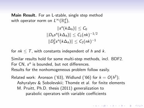
Main Result. For an L-stable, single step methodwith operator norm on L∞(Rd

h),

‖sn(k∆h)‖ ≤ C0

‖Dhsn(k∆h)‖ ≤ C1(nk)−1/2

‖D2hsn(k∆h)‖ ≤ C2(nk)−1

for nk ≤ T , with constants independent of h and k.

Similar results hold for some multi-step methods, incl. BDF2.For CN, sn is bounded, but not differences.Results for the nonhomogeneous problem follow easily.

Related work: Aronson (’63), Widlund (’66) for k = O(h2);Ashyralyev & Sobolevskii; Thomee et al. for finite elementsM. Pruitt, Ph.D. thesis (2011) generalization to

parabolic operators with variable coefficients

Proof of the Main Result

‖sn(k∆h)‖ ≤ C0

‖Dhsn(k∆h)‖ ≤ C1(nk)−1/2

‖D2hsn(k∆h)‖ ≤ C2(nk)−1

Use the point of view of analytic semigroups, as inThomee, Galerkin FEM for Parabolic ProblemsAshyralyev & Sobolevskii, ...Parabolic Difference Eq’ns

Proof in three steps:(1) For the semidiscrete equation ut = ∆hu , u = u(jh, t)

estimate u and its differences for complex t,‖Dm

h e∆ht‖ ≤ Cm|t|−m/2 on L∞(Rdh)

(2) Estimate Dmh (z −∆h)−1 using (1).

(3) Write sn(z) as a contour integral using (z −∆h)−1;estimate Dm

h sn(z) on L∞(Rdh) for n large.

Step 1. Semidiscrete: ut = ∆hu , u(t) = e∆htu0

Show ‖Dmh e∆ht‖ ≤ Cm|t|−m/2 on L∞(Rd

h), for complex tt in a sector, t = t1 + it2 : t1 > 0, |t2| ≤ Mt1

Use gt = ∆hg , g(jh, 0) = δj0

u(jh, t) =∑

` g(jh − `h, t)u0(`h)

Estimate Dmh g in discrete L1 using transform (F. John, ’52)

f (jh) =1

2π

∫ π

−πf (ξ)e ijξ dξ , f (ξ) =

∑j∈Z

f (jh)e−ijξ

in one dimension; g(ξ, t) = exp(−4t sin2(ξ/2)/h2) ; e.g.,

|g(jh, t)| ≤ C

j2

∫ π

−π|g ′′(ξ, t)| dξ ≤ C ′

j2

|t|1/2

h(D+

h g)

(ξ) = (2i/h) e iξ/2 sin(ξ/2)g(ξ)

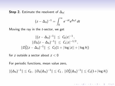
Step 2. Estimate the resolvent of ∆h:

(z −∆h)−1 =

∫ ∞0

e−zte∆ht dt

Moving the ray in the t-sector, we get

‖(z −∆h)−1‖ ≤ C0|z |−1 ,

‖Dh(z −∆h)−1‖ ≤ C1|z |−1/2 ,

‖D2h(z −∆h)−1‖ ≤ C2(1 + | log |z ||+ | log h|)

for z outside a sector about z < 0

For periodic functions, mean value zero,

‖(∆h)−1‖ ≤ C0 , ‖Dh(∆h)−1‖ ≤ C1 , ‖D2h(∆h)−1‖ ≤ C2(1+| log h|)

Proof of the Main Result

Step 3. Estimate s(k∆h)n and differences:

Dαh s(k∆h)n =

1

2πi

∫Γs(z)nDα

h (z − k∆h)−1dz

use contour Γ, radius O(1/n)use resolvent estimates

from Step 2use assumptions on s:

s(z) analytic in a sector about z < 0,s(z) = 1 + z + O(z2) as z → 0 ,|s(z)| ≤ (1 + c1|z |)−1 , z in sector about z < 0(from consistency and L-stability)

Discrete Parabolic Operators with VariableCoefficients

Michael Pruitt, Ph.D. Thesis (2011)E.g., ut = D+

h

(a(x , h)D−h u

), u(·, 0) given

Similar results with gain of regularity in maximum normSteps 2 and 3 are similar, once Step 1 is doneMain part: Step 1, estimating semidiscrete equationNeed estimates for u, Dhu, D2

hu for complex tFundamental solution from construction of E. E. Levi

LhΓh(x , t; y) = 0 , Γh(x , 0; y) = δxy

so that u(x , t) =∑

x ′ Γh(x , t; x ′)u0(x ′)Cf. recent work of A. Mazzucato

Lh = parabolic operator; Γh is the fund’l sol’n,

LhΓh(x , t; y) = 0 , Γh(x , 0; y) = δxy

Estimates for Γ, t in a sector about t > 0 in C:

|Dγh Γh(x , t; y)| ≤ C1h

d |t|−d/2−|γ|/2e−C2|x−y |/√|t|eωt , |t| ≥ h2

|Dγh Γh(x , t; y)| ≤ C1h

−|γ|e−C2|x−y |/heωt , |t| ≤ 2h2

Start with frozen coefficient problem; fix y , coeff’ts at y ,

Lh(y)Gh(x , t; y) = 0 , Gh(x , 0; y) = δx0

First prove that Gh has the estimates stated for Γh

using the discrete Fourier transform, complex extension

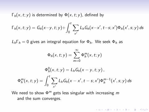
Γh(x , t; y) is determined by Φ(x , t; y), defined by

Γh(x , t; y) = Gh(x−y , t; y)+

∫ t

0

∑x ′

LhGh(x−x ′, t−s; x ′)Φh(x ′, s; y) ds

LhΓh = 0 gives an integral equation for Φh. We seek Φh as

Φh(x , t; y) =∞∑

m=0

Φmh (x , t; y)

Φ0h(x , t; y) = LhGh(x − y , t; y) ,

Φmh (x , t; y) =

∫ t

0

∑x ′

LhGh(x − x ′, t − s; x ′)Φm−1h (x ′, s; y) ds

We need to show Φm gets less singular with increasing mand the sum converges.

Estimates for Φm :They depend on α in Holder condition for coeff’ts.Power of |t| increases by α/2 at each step.For |t| ≥ h2, m ≥ 0

|Φmh (x , t; y)| ≤ C (m)hd |t|−d/2−1+(m+1)α/2e−C2|x−y |/

√|t|eω|t|

For large m,

C (m) =Cm

Γ((m + 1)α/2− d/2)

Prototype Problem, Interface in Viscous Fluid

Navier-Stokes equationsinterface Γ : X(α, t)α = material coordinates = arclength at current timerestoring force on Γ acts on fluidperiodic b.c.’s on box

−

+

ΩΩ Γ

∂u

∂t+ u · ∇u = −∇p + µ∆u + fδΓ ,

∇ · u = 0 , τ = unit tangent,

f(s, t) =∂

∂s(T (s, t)τ (s, t)) ,

T (s, t) = T0

(∣∣∣∣∂X

∂α

∣∣∣∣− 1

).

interfacial force amounts to jumps in ∇u and p

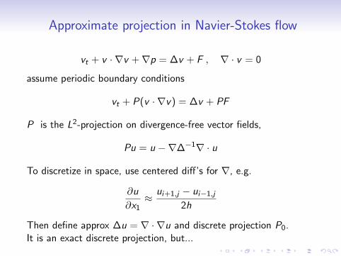
Approximate projection in Navier-Stokes flow

vt + v · ∇v +∇p = ∆v + F , ∇ · v = 0

assume periodic boundary conditions

vt + P(v · ∇v) = ∆v + PF

P is the L2-projection on divergence-free vector fields,

Pu = u −∇∆−1∇ · u

To discretize in space, use centered diff’s for ∇, e.g.

∂u

∂x1≈

ui+1,j − ui−1,j

2h

Then define approx ∆u = ∇ · ∇u and discrete projection P0.It is an exact discrete projection, but...

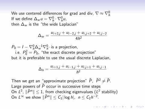
We use centered differences for grad and div, ∇ ≈ ∇0h

If we define ∆wu = ∇0h · ∇0

hu,then ∆w is the “the wide Laplacian”

∆w =ui+2,j + ui−2,j + ui ,j+2 + ui ,j−2

4h2

P0 = I −∇0h∆−1

w ∇0h· is a projection,

i.e. P20 = P0, “the exact discrete projection”

but it is preferable to use the usual discrete Laplacian,

∆h =ui+1,j + ui−1,j + ui ,j+1 + ui ,j−1

h2

Then we get an “approximate projection” P, P2 6= P.Large powers of P occur in successive time stepsOn L2, ‖Pn‖ ≤ 1, from checking eigenvalues (L2 stability)On L∞ we show ‖Pn‖ ≤ C1| log h|, n ≤ C2h

−2.

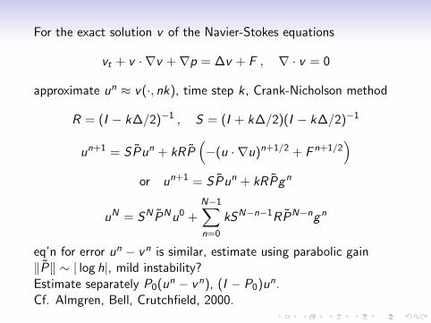
For the exact solution v of the Navier-Stokes equations

vt + v · ∇v +∇p = ∆v + F , ∇ · v = 0

approximate un ≈ v(·, nk), time step k , Crank-Nicholson method

R = (I − k∆/2)−1 , S = (I + k∆/2)(I − k∆/2)−1

un+1 = SPun + kRP(−(u · ∇u)n+1/2 + F n+1/2

)or un+1 = SPun + kRPgn

uN = SN PNu0 +N−1∑n=0

kSN−n−1RPN−ngn

eq’n for error un − vn is similar, estimate using parabolic gain‖P‖ ∼ | log h|, mild instability?Estimate separately P0(un − vn), (I − P0)un.Cf. Almgren, Bell, Crutchfield, 2000.

Estimating the approximate projection

We show ‖Pn‖ ≤ C1| log h| on L∞, n ≤ C2h−2.

Discrete Fourier transform, periodic grid functions

f (k) =∑

j

f (jh)e−ikjh , f (jh) = (2π)−d∑k

f (k)e ikjhhd .

|jν | ≤ π/h, |kν | ≤ π/h, 1 ≤ ν ≤ d

For an operator A, multiplying in transform,

(Af ) (k) = σ(kh)f (k)

we can estimate the operator norm on L∞ by (s > d/2)

‖A‖ ≤ C1‖(D+)sσ‖d2s

L2h‖σ‖1− d

2s

L2h

+ C2‖σ‖L2h.

Approximate projection P = I −∇0h∆−1

h ∇0h·

The difference operators have symbols in the discrete transform

(D0ν ) =

i

hsin ξν ξ = kh

(∆h) (ξ) = − 4

h2

(sin2(ξ1/2) + sin2(ξ2/2)

)(Take d = 2.) The symbol of P is

a 2× 2 matrix σ(ξ) with eigenvalues

λ0 =s4

1 + s42

s21 + s2

2

, λ1 = 1 , si = sin(ξi/2)

Estimating Pn reduces to estimating the nth power ofthe (scalar) operator with symbol λ0.