relativistic fluid dynamics: physics for many different · pdf filerelativistic fluid...
TRANSCRIPT

arX
iv:g
r-qc
/060
5010
v2 2
May
200
6
Relativistic fluid dynamics: physics for many different scales
N. Andersson
School of Mathematics
University of Southampton
Southampton SO17 1BJ, United Kingdom
email: [email protected]
G. L. Comer
Department of Physics & Center for Fluids at All Scales
Saint Louis University
St. Louis, MO, 63156-0907, USA
email: [email protected]
February 6, 2008
Abstract
The relativistic fluid is a highly successful model used to describe the dynamics of many-particle, relativistic systems. It takes as input basic physics from microscopic scales and yieldsas output predictions of bulk, macroscopic motion. By inverting the process, an understandingof bulk features can lead to insight into physics on the microscopic scale. Relativistic fluidshave been used to model systems as “small” as heavy ions in collisions, and as large as theuniverse itself, with “intermediate” sized objects like neutron stars being considered alongthe way. The purpose of this review is to discuss the mathematical and theoretical physicsunderpinnings of the relativistic (multiple) fluid model. We focus on the variational principleapproach championed by Brandon Carter and his collaborators, in which a crucial elementis to distinguish the momenta that are conjugate to the particle number density currents.This approach differs from the “standard” text-book derivation of the equations of motionfrom the divergence of the stress-energy tensor, in that one explicitly obtains the relativisticEuler equation as an “integrability” condition on the relativistic vorticity. We discuss theconservation laws and the equations of motion in detail, and provide a number of (in ouropinion) interesting and relevant applications of the general theory.
1

1 Introduction
1.1 Setting the stage
If one does a search on the topic of relativistic fluids on any of the major physics article databasesone is overwhelmed by the number of “hits”. This is a manifestation of the importance thatthe fluid model has long had for modern physics and engineering. For relativistic physics, inparticular, the fluid model is essential. After all, many-particle astrophysical and cosmologicalsystems are the best sources of detectable effects associated with General Relativity. Two obviousexamples, the expansion of the universe and oscillations of neutron stars, indicate the vast rangeof scales on which relativistic fluid models are relevant. A particularly exciting context for generalrelativistic fluids today is their use in the modelling of sources of gravitational waves. This includesthe compact binary inspiral problem, either of two neutron stars or a neutron star and a blackhole, the collapse of stellar cores during supernovae, or various neutron star instabilities. Oneshould also not forget the use of special relativistic fluids in modelling collisions of heavy nuclei,astrophysical jets, and gamma-ray burst sources.
This review provides an introduction to the modelling of fluids in General Relativity. Ourmain target audience is graduate students with a need for an understanding of relativistic fluiddynamics. Hence, we have made an effort to keep the presentation pedagogical. The articlewill (hopefully) also be useful to researchers who work in areas outside of General Relativity andgravitation per se (eg. a nuclear physicist who develops neutron star equations of state), but whorequire a working knowledge of relativistic fluid dynamics.
Throughout most of the article we will assume that General Relativity is the proper descriptionof gravity. Although not too severe, this is a restriction since the problem of fluids in othertheories of gravity has interesting aspects. As we hope that the article will be used by studentsand researchers who are not necessarily experts in General Relativity and techniques of differentialgeometry, we have included some discussion of the mathematical tools required to build models ofrelativistic objects. Even though our summary is not a proper introduction to General Relativitywe have tried to define the tools that are required for the discussion that follows. Hopefullyour description is sufficiently self-contained to provide a less experienced reader with a workingunderstanding of (at least some of) the mathematics involved. In particular, the reader will findan extended discussion of the covariant and Lie derivatives. This is natural since many importantproperties of fluids, both relativistic and non-relativistic, can be established and understood by theuse of parallel transport and Lie-dragging. But it is vital to appreciate the distinctions betweenthe two.
Ideally, the reader should have some familiarity with standard fluid dynamics, eg. at the levelof the discussion in Landau & Lifshitz [62], basic thermodynamics [91], and the mathematics ofaction principles and how they are used to generate equations of motion [61]. Having statedthis, it is clear that we are facing a facing a real challenge. We are trying to introduce a topicon which numerous books have been written (eg. [106, 62, 67, 8, 117]), and which requires anunderstanding of much of theoretical physics. Yet, one can argue that an article of this kind istimely. In particular, there has recently been exciting developments for multi-constituent systems,such as superfluid/superconducting neutron star cores.1 Much of this work has been guided by thegeometric approach to fluid dynamics championed by Carter [14, 16, 18]. This provides a powerfulframework that makes extensions to multi-fluid situations quite intuitive. A typical example of aphenomenon that arises naturally is the so-called entrainment effect, which plays a crucial role ina superfluid neutron star core. Given the potential for future applications of this formalism, we
1In this article we use “superfluid” to refer to any system which has the ability to flow without friction. In this
sense, superfluids and superconductors are viewed in the same way. When we wish to distinguish charge carrying
fluids, we will call them superconductors.
2
have opted to base much of our description on the work of Carter and his colleagues.Even though the subject of relativistic fluids is far from new, a number of issues remain to be
resolved. The most obvious shortcoming of the present theory concerns dissipative effects. As wewill discuss, dissipative effects are (at least in principle) easy to incorporate in Newtonian theorybut the extension to General Relativity is problematic (see, for instance, Hiscock and Lindblom[51]). Following early work by Eckart [36], a significant effort was made by Israel and Stewart[55, 54] and Carter [14, 16]. Incorporation of dissipation is still an active enterprise, and of keyimportance for future gravitational-wave asteroseismology which requires detailed estimates of therole of viscosity in suppressing possible instabilities.
1.2 A brief history of fluids
The two fluids air and water are essential to human survival. This obvious fact implies a basichuman need to divine their innermost secrets. Homo Sapiens have always needed to anticipate airand water behaviour under a myriad of circumstances, such as those that concern water supply,weather, and travel. The essential importance of fluids for survival, and that they can be exploitedto enhance survival, implies that the study of fluids probably reaches as far back into antiquityas the human race itself. Unfortunately, our historical record of this ever-ongoing study is not sogreat that we can reach very far accurately.
A wonderful account (now in Dover print) is “A History and Philosophy of Fluid Mechanics,”by G. A. Tokaty [105]. He points out that while early cultures may not have had universities,government sponsored labs, or privately funded centres pursuing fluids research (nor the LivingReviews archive on which to communicate results!), there was certainly some collective understand-ing. After all, there is a clear connection between the viability of early civilizations and their accessto water. For example, we have the societies associated with the Yellow and Yangtze rivers inChina, the Ganges in India, the Volga in Russia, the Thames in England, and the Seine in France,to name just a few. We should also not forget the Babylonians and their amazing technological(irrigation) achievements in the land between the Tigris and Euphrates, and the Egyptians, whoseintimacy with the flooding of the Nile is well documented. In North America, we have the so-called Mississippians, who left behind their mound-building accomplishments. For example, theCahokians (in Collinsville, Illinois) constructed Monk’s Mound, the largest precolumbian earthenstructure in existence that is (see http://en.wikipedia.org/wiki/Monk’s_Mound) “... over 100feet tall, 1000 feet long, and 800 feet wide (larger at its base than the Great Pyramid of Giza).”
In terms of ocean and sea travel, we know that the maritime ability of the Mediterranean peoplewas a main mechanism for ensuring cultural and economic growth and societal stability. The finely-tuned skills of the Polynesians in the South Pacific allowed them to travel great distances, perhapsreaching as far as South America itself, and certainly making it to the “most remote spot on theEarth,” Easter Island. Apparently, they were remarkably adept at reading the smallest of signs— water color, views of weather on the horizon, subtleties of wind patterns, floating objects, birds,etc — as indication of nearby land masses. Finally, the harsh climate of the North Atlantic wasovercome by the highly accomplished Nordic sailors, whose skills allowed them to reach severalsites in North America. Perhaps it would be appropriate to think of these early explorers as adeptgeophysical fluid dynamicists/oceanographers?
Many great scientists are associated with the study of fluids. Lost are the names of thoseindividuals who, almost 400,000 years ago, carved “aerodynamically correct” [43] wooden spears.Also lost are those who developed boomerangs and fin-stabilized arrows. Among those not lost isArchimedes, the Greek Mathematician (287-212 BC), who provided a mathematical expression forthe buoyant force on bodies. Earlier, Thales of Miletus (624-546 BC) asked the simple question:What is air and water? His question is profound since it represents a clear departure from themain, myth-based modes of inquiry at that time. Tokaty ranks Hero of Alexandria as one of the
3

Leonardo da Vinci(1425-1519)
Isaac Newton(1642-1727)
Leonhard Euler
Louis de Lagrange(1707-83)
(1736-1813)
Andre Lichnerowicz(1915-1998)
(1879-1955)
Albert Einstein
Sophus Lie(1842-1899)
Heike Kamerlingh-Onnes(1853-1926)
Carl Henry Eckart(1902-1973)
Lev Davidovich Landau(1908-1968)
Lars Onsager(1903-1976)
(1931-)
(1947-)
Werner Israel
John M. Stewart
Brandon Carter(1942-)
EARLY EMPIRICAL STUDIES
1700s FLUID DYNAMICS
VARIATIONAL METHODS
1900s RELATIVITY
VORTICITY
IRREVERSIBLE THERMODYNAMICS
1950s SUPERFLUIDS
RELATIVISTIC DISSIPATION
MULTIFLUID MODELS
Isaak Markovich Khalatnikov(1919-)
1800s VISCOSITY
Ilya Prigogine(1917-2003)
Claude Louis Navier(1785-1836)
George Gabriel Stokes(1819-1903)
Daniel Bernoulli(1700-1782)
Hans Ertel(1904-1995)
Archimedes(287-212 BC)
Figure 1: A “timeline” focussed on the topics covered in this review, including chemists, engineers,mathematicians, philosophers, and physicists who have contributed to the development of non-relativistic fluids, their relativistic counterparts, multi-fluid versions of both, and exotic phenomenasuch as superfluidity.
great, early contributors. Hero (c. 10-70) was a Greek scientist and engineer, who left behindmany writings and drawings that, from today’s perspective, indicate a good grasp of basic fluidmechanics. To make complete account of individual contributions to our present understandingof fluid dynamics is, of course, impossible. Yet it is useful to list some of the contributors to thefield. We provide a highly subjective “timeline” in Fig. 1. Our list is to a large extent focussed onthe topics covered in this review, and includes chemists, engineers, mathematicians, philosophers,and physicists. It recognizes those who have contributed to the development of non-relativisticfluids, their relativistic counterparts, multi-fluid versions of both, and exotic phenomena such assuperfluidity. We have provided this list with the hope that the reader can use these names askey words in a modern, web-based literature search whenever more information is required.
Tokaty [105] discusses the human propensity for destruction when it comes to our water re-sources. Depletion and pollution are the main offenders. He refers to a “Battle of the Fluids”as a struggle between their destruction and protection. His context for this discussion was theCold War. He rightly points out the failure to protect our water and air resource by the twopredominant participants — the USA and USSR. In an ironic twist, modern study of the rela-tivistic properties of fluids has also a “Battle of the Fluids.” A self-gravitating mass can becomeabsolutely unstable and collapse to a black hole, the ultimate destruction of any form of matter.
1.3 Notation and conventions
Throughout the article we assume the “MTW” [75] conventions. We also generally assume ge-ometrized units c = G = 1, unless specifically noted otherwise. A coordinate basis will always beused, with spacetime indices denoted by lowercase Greek letters that range over 0, 1, 2, 3 (timebeing the zeroth coordinate), and purely spatial indices denoted by lowercase Latin letters that
4

range over 1, 2, 3. Unless otherwise noted, we assume the Einstein summation convention.
5
2 Physics in a Curved Spacetime
There is an extensive literature on special and general relativity, and the spacetime-based view(i.e. three space and one time dimensions that form a manifold) of the laws of physics. Forthe student at any level interested in developing a working understanding we recommend Taylorand Wheeler [103] for an introduction, followed by Hartle’s excellent recent text [48] designed forstudents at the undergraduate level. For the more advanced students, we suggest two of theclassics, “MTW” [75] and Weinberg [111], or the more contemporary book by Wald [108]. Finally,let us not forget the Living Reviews archive as a premier online source of up-to-date information!
In terms of the experimental and/or observational support for special and general relativity, werecommend two articles by Will that were written for the 2005 World Year of Physics celebration[115, 116]. They summarize a variety of tests that have been designed to expose breakdownsin both theories. (We also recommend Will’s popular book Was Einstein Right? [113] and histechnical exposition Theory and Experiment in Gravitational Physics [114].) To date, Einstein’stheoretical edifice is still standing!
For special relativity, this is not surprising, given its long list of successes: explanation of theMichaelson-Morley result, the prediction and subsequent discovery of anti-matter, and the standardmodel of particle physics, to name a few. Will [115] offers the observation that genetic mutationsvia cosmic rays require special relativity, since otherwise muons would decay before making it tothe surface of the Earth. On a more somber note, we may consider the Trinity site in New Mexico,and the tragedies of Hiroshima and Nagasaki, as reminders of E = mc2.
In support of general relativity, there are Eotvos-type experiments testing the equivalence ofinertial and gravitational mass, detection of gravitational red-shifts of photons, the passing ofthe solar system tests, confirmation of energy loss via gravitational radiation in the Hulse-Taylorbinary pulsar, and the expansion of the universe. Incredibly, general relativity even finds apractical application in the GPS system: if general relativity is neglected an error of about 15meters results when trying to resolve the location of an object [115]. Definitely enough to makedriving dangerous!
The evidence is thus overwhelming that general relativity, or at least something that passes thesame tests, is the proper description of gravity. Given this, we assume the Einstein EquivalencePrinciple, i.e. that [115, 116, 114]:
• test bodies fall with the same acceleration independently of their internal structure or com-position;
• the outcome of any local non-gravitational experiment is independent of the velocity of thefreely-falling reference frame in which it is performed;
• the outcome of any local non-gravitational experiment is independent of where and when inthe universe it is performed.
If the Equivalence Principle holds, then gravitation must be described by a metric-based theory[115]. This means that
1. spacetime is endowed with a symmetric metric,
2. the trajectories of freely falling bodies are geodesics of that metric, and
3. in local freely falling reference frames, the non-gravitational laws of physics are those ofspecial relativity.
For our present purposes this is very good news. The availability of a metric means that wecan develop the theory without requiring much of the differential geometry edifice that would be
6

needed in a more general case. We will develop the description of relativistic fluids with this inmind. Readers that find our approach too “pedestrian” may want to consult the recent article byGourgoulhon [46], which serves as a useful complement to our description.
2.1 The Metric and Spacetime Curvature
Our strategy is to provide a “working understanding” of the mathematical objects that enter theEinstein equations of general relativity. We assume that the metric is the fundamental “field”of gravity. For four-dimensional spacetime it determines the distance between two spacetimepoints along a given curve, which can generally be written as a one parameter function with,say, components xµ(λ). As we will see, once a notion of parallel transport is established, themetric also encodes information about the curvature of its spacetime, which is taken to be of thepseudo-Riemannian type, meaning that the signature of the metric is −+ ++ (cf. Eq. (2) below).
In a coordinate basis, which we will assume throughout this review, the metric is denoted bygµν = gνµ. The symmetry implies that there are in general ten independent components (modulothe freedom to set arbitrarily four components that is inherited from coordinate transformations;cf. Eqs. (8) and (9) below). The spacetime version of the Pythagorean theorem takes the form
ds2 = gµνdxµdxν , (1)
and in a local set of Minkowski coordinates t, x, y, z (i.e. in a local inertial frame) it looks like
ds2 = − (dt)2+ (dx)
2+ (dy)
2+ (dz)
2. (2)
This illustrates the − + ++ signature. The inverse metric gµν is such that
gµρgρν = δµν , (3)
where δµν is the unit tensor. The metric is also used to raise and lower spacetime indices, i.e. if we
let V µ denote a contravariant vector, then its associated covariant vector (also known as a covectoror one-form) Vµ is obtained as
Vµ = gµνV ν ⇔ V µ = gµνVν . (4)
We can now consider three different classes of curves: timelike, null, and spacelike. A vector issaid to be timelike if gµνV µV ν < 0, null if gµνV µV ν = 0, and spacelike if gµνV µV ν > 0. We cannaturally define timelike, null, and spacelike curves in terms of the congruence of tangent vectorsthat they generate. A particularly useful timelike curve for fluids is one that is parameterized bythe so-called proper time, i.e. xµ(τ) where
dτ2 = −ds2 . (5)
The tangent uµ to such a curve has unit magnitude; specifically,
uµ ≡ dxµ
dτ, (6)
and thus
gµνuµuν = gµν
dxµ
dτ
dxν
dτ=
ds2
dτ2= −1 . (7)
Under a coordinate transformation xµ → xµ, contravariant vectors transform as
Vµ
=∂xµ
∂xνV ν (8)
7

and covariant vectors as
V µ =∂xν
∂xµ Vν . (9)
Tensors with a greater rank (i.e. a greater number of indices), transform similarly by acting linearlyon each index using the above two rules.
When integrating, as we need to when we discuss conservation laws for fluids, we must becareful to have an appropriate measure that ensures the coordinate invariance of the integration.In the context of three-dimensional Euclidean space the measure is referred to as the Jacobian.For spacetime, we use the so-called volume form ǫµνρτ . It is completely antisymmetric, and forfour-dimensional spacetime, it has only one independent component, which is
ǫ0123 =√−g and ǫ0123 =
1√−g, (10)
where g is the determinant of the metric. The minus sign is required under the square root becauseof the metric signature. By contrast, for three-dimensional Euclidean space (i.e. when consideringthe fluid equations in the Newtonian limit) we have
ǫ123 =√
g and ǫ123 =1√g
, (11)
where g is the determinant of the three-dimensional space metric. A general identity that isextremely useful is [108]
ǫµ1...µjµj+1...µnǫµ1...µjνj+1...νn= (−1)s (n − j)!j!δ[µj+1 . . .
νj+1δµn ]
νn(12)
where s is the number of minus signs in the metric (eg. s = 1 here). As an application considerthree-dimensional, Euclidean space. Then s = 0 and n = 3. Using lower-case Latin indices wesee (for j = 1 in Eq. (12))
ǫmijǫmkl = δikδj
l − δjkδi
l . (13)
The general identity will be used in our discussion of the variational principle, while the three-dimensional version is often needed in discussions of Newtonian vorticity.
2.2 Parallel Transport and the Covariant Derivative
In order to have a generally covariant prescription for fluids, i.e. written in terms of spacetimetensors, we must have a notion of derivative ∇µ that is itself covariant. For example, when ∇µ
acts on a vector V ν a rank-two tensor of mixed indices must result:
∇µVν
=∂xσ
∂xµ
∂xν
∂xρ∇σV ρ . (14)
The ordinary partial derivative does not work because under a general coordinate transformation
∂Vν
∂xµ =∂xσ
∂xµ
∂xν
∂xρ
∂V ρ
∂xσ+
∂xσ
∂xµ
∂2xν
∂xσ∂xρV ρ . (15)
The second term spoils the general covariance, since it vanishes only for the restricted set ofrectilinear transformations
xµ = aµνxν + bµ , (16)
where aµν and bµ are constants.
For both physical and mathematical reasons, one expects a covariant derivative to be defined interms of a limit. This is, however, a bit problematic. In three-dimensional Euclidean space limits
8

a) b)
Figure 2: A schematic illustration of two possible versions of parallel transport. In the first case(a) a vector is transported along great circles on the sphere locally maintaining the same angle withthe path. If the contour is closed, the final orientation of the vector will differ from the originalone. In case (b) the sphere is considered to be embedded in a three-dimensional Euclidean space,and the vector on the sphere results from projection. In this case, the vector returns to the originalorientation for a closed contour.
can be defined uniquely in that vectors can be moved around without their lengths and directionschanging, for instance, via the use of Cartesian coordinates, the i, j,k set of basis vectors, and theusual dot product. Given these limits those corresponding to more general curvilinear coordinatescan be established. The same is not true of curved spaces and/or spacetimes because they do nothave an a priori notion of parallel transport.
Consider the classic example of a vector on the surface of a sphere (illustrated in Fig. 2). Takethat vector and move it along some great circle from the equator to the North pole in such a wayas to always keep the vector pointing along the circle. Pick a different great circle, and withoutallowing the vector to rotate, by forcing it to maintain the same angle with the locally straightportion of the great circle that it happens to be on, move it back to the equator. Finally, movethe vector in a similar way along the equator until it gets back to its starting point. The vector’sspatial orientation will be different from its original direction, and the difference is directly relatedto the particular path that the vector followed.
On the other hand, we could consider that the sphere is embedded in a three-dimensionalEuclidean space, and that the two-dimensional vector on the sphere results from projection of athree-dimensional vector. Move the projection so that its higher-dimensional counterpart alwaysmaintains the same orientation with respect to its original direction in the embedding space. Whenthe projection returns to its starting place it will have exactly the same orientation as it startedwith, see Fig. 2. It is thus clear that a derivative operation that depends on comparing a vectorat one point to that of a nearby point is not unique, because it depends on the choice of paralleltransport.
Pauli [83] notes that Levi-Civita [66] is the first to have formulated the concept of parallel“displacement,” with Weyl [112] generalizing it to manifolds that do not have a metric. The pointof view expounded in the books of Weyl and Pauli is that parallel transport is best defined as amapping of the “totality of all vectors” that “originate” at one point of a manifold with the totality
9

at another point. (In modern texts, one will find discussions based on fiber bundles.) Pauli pointsout that we cannot simply require equality of vector components as the mapping.
Let us examine the parallel transport of the force-free, point particle velocity in Euclideanthree-dimensional space as a means for motivating the form of the mapping. As the velocity isconstant, we know that the curve traced out by the particle will be a straight line. In fact, wecan turn this around and say that the velocity parallel transports itself because the path tracedout is a geodesic (i.e. the straightest possible curve allowed by Euclidean space). In our analysiswe will borrow liberally from the excellent discussion of Lovelock and Rund [71]. Their text iscomprehensive yet readable for one who is not well-versed with differential geometry. Finally,we note that this analysis will be of use later when we obtain the Newtonian limit of the generalrelativistic equations, but in an arbitrary coordinate basis.
We are all well aware that the points on the curve traced out by the particle are describable, inCartesian coordinates, by three functions xi(t) where t is the standard Newtonian time. Likewise,we know the tangent vector at each point of the curve is given by the velocity components vi(t) =dxi/dt, and that the force-free condition is equivalent to
ai(t) =dvi
dt= 0 ⇒ vi(t) = const . (17)
Hence, the velocity components vi(0) at the point xi(0) are equal to those at any other point alongthe curve, say vi(T ) at xi(T ), and so we could simply take vi(0) = vi(T ) as the mapping. But asPauli warns, we only need to reconsider this example using spherical coordinates to see that thevelocity components r, θ, φ must necessarily change as they undergo parallel transport along astraight-line path (assuming the particle does not pass through the origin). The question is whatshould be used in place of component equality? The answer follows once we find a curvilinearcoordinate version of dvi/dt = 0.
What we need is a new “time” derivative D/dt, that yields a generally covariant statement
Dvi
dt= 0 , (18)
where the vi(t) = dxi/dt are the velocity components in a curvilinear system of coordinates. Letus consider an infinitesimal displacement of the velocity from xi(t) to xi(t + δt). In Cartesiancoordinates we know that
δvi =∂vi
∂xjδxj = 0 . (19)
Consider now a coordinate transformation to the curvilinear coordinate system xi, the inversebeing xi = xi(xj). Given that
vi =∂xi
∂xjvj (20)
we can writedvi
dt=
(
∂xi
∂xj
∂vj
∂xk+
∂2xi
∂xk∂xjvj
)
vk . (21)
The metric gij for our curvilinear coordinate system is obtainable from
gij =∂xk
∂xi
∂xl
∂xjgkl , (22)
where
gij =
1 i = j0 i 6= j
. (23)
10

Differentiating Eq. (22) with respect to x, and permuting indices, we can show that
∂2xh
∂xi∂xj
∂xl
∂xkghl =
1
2
(
gik,j + gjk,i − gij,k
)
≡ gil
l
j k
, (24)
where
gij,k ≡ ∂gij
∂xk. (25)
With some tensor algebra we find
dvi
dt=
∂xi
∂xj
Dvi
dt, (26)
whereDvi
dt= vj
(
∂vi
∂xj+
ik j
vk
)
. (27)
One can verify that the operator D/dt is covariant with respect to general transformations ofcurvilinear coordinates.
We now identify our generally covariant derivative (dropping the overline) as
∇jvi =
∂vi
∂xj+
ik j
vk ≡ vi;j . (28)
Similarly, the covariant derivative of a covector is
∇jvi =∂vi
∂xj−
ki j
vk ≡ vi;j . (29)
One extends the covariant derivative to higher rank tensors by adding to the partial derivativeeach term that results by acting linearly on each index with
i
k j
using the two rules given above.By relying on our understanding of the force-free point particle, we have built a notion of
parallel transport that is consistent with our intuition based on equality of components in Cartesiancoordinates. We can now expand this intuition and see how the vector components in a curvilinearcoordinate system must change under an infinitesimal, parallel displacement from xi(t) to xi(t+δt).Setting Eq. (27) to zero, and noting that viδt = δxi, implies
δvi ≡ ∂vi
∂xjδxj = −
i
k j
vkδxj . (30)
In general relativity we assume that under an infinitesimal parallel transport from a spacetimepoint xµ(λ) on a given curve to a nearby point xµ(λ + δλ) on the same curve, the components ofa vector V µ will change in an analogous way, namely
δV µ
‖ ≡ ∂V µ
∂xνδxν = −Γµ
ρνV ρδxν , (31)
where
δxµ ≡ dxν
dλδλ . (32)
Weyl [112] refers to the symbol Γµρν as the “components of the affine relationship,” but we will use
the modern terminology and call it the connection. In the language of Weyl and Pauli, this is themapping that we were looking for.
For Euclidean space, we can verify that the metric satisfies
∇igjk = 0 (33)
11

for a general, curvilinear coordinate system. The metric is thus said to be “compatible” with thecovariant derivative. We impose metric compatibility in general relativity. This results in theso-called Christoffel symbol for the connection, defined as
Γρµν =
1
2gρσ (gµσ,ν + gνσ,µ − gµν,σ) . (34)
The rules for the covariant derivative of a contravariant vector and a covector are the same as inEqs. (28) and (29), except that all indices are for full spacetime.
2.3 The Lie Derivative and Spacetime Symmetries
Another important tool for measuring changes in tensors from point to point in spacetime is theLie derivative. It requires a vector field, but no connection, and is a more natural definition inthe sense that it does not even require a metric. It yields a tensor of the same type and rankas the tensor on which the derivative operated (unlike the covariant derivative, which increasesthe rank by one). The Lie derivative is as important for Newtonian, non-relativistic fluids as forrelativistic ones (a fact which needs to be continually emphasized as it has not yet permeated thefluid literature for chemists, engineers, and physicists). For instance, the classic papers on theChandrasekhar-Friedman-Schutz instability [41, 42] in rotating stars are great illustrations of theuse of the Lie derivative in Newtonian physics. We recommend the book by Schutz [98] for acomplete discussion and derivation of the Lie derivative and its role in Newtonian fluid dynamics(see also the recent series of papers by Carter and Chamel [19, 20, 21]). We will adapt here thecoordinate-based discussion of Schouten [94], as it may be more readily understood by those notwell-versed in differential geometry.
In a first course on classical mechanics, when students encounter rotations, they are introducedto the idea of active and passive transformations. An active transformation would be to fix theorigin and axis-orientations of a given coordinate system with respect to some external observer,and then move an object from one point to another point of the same coordinate system. A passivetransformation would be to place an object so that it remains fixed with respect to some externalobserver, and then induce a rotation of the object with respect to a given coordinate system, byrotating the coordinate system itself with respect to the external observer. We will derive the Liederivative of a vector by first performing an active transformation and then following this witha passive transformation and finding how the final vector differs from its original form. In thelanguage of differential geometry, we will first “push-forward” the vector, and then subject it to a“pull-back”.
In the active, push-forward sense we imagine that there are two spacetime points connected bya smooth curve xµ(λ). Let the first point be at λ = 0, and the second, nearby point at λ = ǫ,i.e. xµ(ǫ); that is,
xµǫ ≡ xµ(ǫ) ≈ xµ
0 + ǫ ξµ , (35)
where xµ0 ≡ xµ(0) and
ξµ =dxµ
dλ
∣
∣
∣
∣
λ=0
(36)
is the tangent to the curve at λ = 0. In the passive, pull-back sense we imagine that the coordinatesystem itself is changed to xµ = xµ(xν), but in the very special form
xµ = xµ − ǫ ξµ . (37)
It is in this last step that the Lie derivative differs from the covariant derivative. In fact, if weinsert Eq. (35) into (37) we find the result xµ
ǫ = xµ0 . This is called “Lie-dragging” of the coordinate
12

xm
xm
xm(l)
l=0
l=e
Figure 3: A schematic illustration of the Lie derivative. The coordinate system is dragged alongwith the flow, and one can imagine an observer “taking derivatives” as he/she moves with the flow(see the discussion in the text).
frame, meaning that the coordinates at λ = 0 are carried along so that at λ = ǫ, and in the newcoordinate system, the coordinate labels take the same numerical values.
As an interesting aside it is worth noting that Arnold [9], only a little whimsically, refers to thisconstruction as the “fisherman’s derivative”. He imagines a fisherman sitting in a boat on a river,“taking derivatives” as the boat moves with the current. Playing on this imagery, the covariantderivative is cast with the high-test Zebco parallel transport fishing pole, the Lie derivative withthe Shimano, Lie-dragging ultra-light. Let us now see how Lie-dragging reels in vectors.
For some given vector field that takes values V µ(λ), say, along the curve, we write
V µ0 = V µ(0) (38)
for the value of V µ at λ = 0 andV µ
ǫ = V µ(ǫ) (39)
for the value at λ = ǫ. Because the two points xµ0 and xµ
ǫ are infinitesimally close ǫ << 1, and wecan thus write
V µǫ ≈ V µ
0 + ǫ ξν ∂V µ
∂xν
∣
∣
∣
∣
λ=0
, (40)
for the value of V µ at the nearby point and in the same coordinate system. However, in the newcoordinate system at the nearby point, we find
V µǫ =
(
∂xµ
∂xνV ν
)∣
∣
∣
∣
λ=ǫ
≈ V µǫ − ǫ V ν
0
∂ξµ
∂xν
∣
∣
∣
∣
λ=0
. (41)
The Lie derivative now is defined to be
LξVµ = lim
ǫ→0
V µǫ − V µ
ǫ
= ξν ∂V µ
∂xν− V ν ∂ξµ
∂xν
13

= ξν∇νV µ − V ν∇νξµ , (42)
where we have dropped the “0” subscript and the last equality follows easily by noting Γρµν = Γρ
νµ.We introduced in Eq. (31) the effect of parallel transport on vector components. By contrast,
the Lie-dragging of a vector causes its components to change as
δV µL = LξV
µ ǫ . (43)
We see that if LξVµ = 0, then the components of the vector do not change as the vector is Lie-
dragged. Suppose now that V µ represents a vector field and that there exists a correspondingcongruence of curves with tangent given by ξµ. If the components of the vector field do not changeunder Lie-dragging we can show that this implies a symmetry, meaning that a coordinate systemcan be found such that the vector components will not depend on one of the coordinates. This isa potentially very powerful statement.
Let ξµ represent the tangent to the curves drawn out by, say, the µ = a coordinate. Then wecan write xa(λ) = λ which means
ξµ = δµa . (44)
If the Lie derivative of V µ with respect to ξν vanishes we find
ξν ∂V µ
∂xν= V ν ∂ξµ
∂xν= 0 . (45)
Using this in Eq. (40) implies V µǫ = V µ
0 , that is to say, the vector field V µ(xν) does not dependon the xa coordinate. Generally speaking, every ξµ that exists that causes the Lie derivative of avector to vanish represents a symmetry.
2.4 Spacetime Curvature
The main message of the previous two subsections is that one must have an a priori idea ofhow vectors and higher rank tensors are moved from point to point in spacetime. Anothermanifestation of the complexity associated with carrying tensors about in spacetime is that thecovariant derivative does not commute. For a vector we find
∇ρ∇σV µ −∇σ∇ρVµ = Rµ
νρσV ν , (46)
where Rµνρσ is the Riemann tensor. It is obtained from
Rµνρσ = Γµ
νσ,ρ − Γµνρ,σ + Γµ
τρΓτνσ − Γµ
τσΓτνρ . (47)
Closely associated are the Ricci tensor Rνσ = Rσν and scalar R that are defined by the contractions
Rνσ = Rµνµσ , R = gνσRνσ . (48)
We will later also have need for the Einstein tensor, which is given by
Gµν = Rµν − 1
2Rgµν . (49)
It is such that ∇µGµν vanishes identically (this is known as the Bianchi Identity).
A more intuitive understanding of the Riemann tensor is obtained by seeing how its presenceleads to a path-dependence in the changes that a vector experiences as it moves from point topoint in spacetime. Such a situation is known as a “non-integrability” condition, because the
14

result depends on the whole path and not just the initial and final points. That is, it is unlike atotal derivative which can be integrated and thus depends on only the lower and upper limits ofthe integration. Geometrically we say that the spacetime is curved, which is why the Riemanntensor is also known as the curvature tensor.
To illustrate the meaning of the curvature tensor, let us suppose that we are given a surfacethat can be parameterized by the two parameters λ and η. Points that live on this surface willhave coordinate labels xµ(λ, η). We want to consider an infinitesimally small “parallelogram”whose four corners (moving counterclockwise with the first corner at the lower left) are given byxµ(λ, η), xµ(λ, η+δη), xµ(λ+δλ, η+δη), and xµ(λ+δλ, η). Generally speaking, any “movement”towards the right of the parallelogram is effected by varying η, and that towards the top resultsby varying λ. The plan is to take a vector V µ(λ, η) at the lower-left corner xµ(λ, η), paralleltransport it along a λ = constant curve to the lower-right corner at xµ(λ, η + δη) where it willhave the components V µ(λ, η + δη), and end up by parallel transporting V µ at xµ(λ, η + δη) alongan η = constant curve to the upper-right corner at xµ(λ + δλ, η + δη). We will call this path Iand denote the final component values of the vector as V µ
I . We repeat the same process exceptthat the path will go from the lower-left to the upper-left and then on to the upper-right corner.We will call this path II and denote the final component values as V µ
II .Recalling Eq. (31) as the definition of parallel transport, we first of all have
V µ(λ, η + δη) ≈ V µ(λ, η) + δηV µ
‖ (λ, η) = V µ(λ, η) − ΓµνρV
νδηxρ (50)
andV µ(λ + δλ, η) ≈ V µ(λ, η) + δλV µ
‖ (λ, η) = V µ(λ, η) − ΓµνρV
νδλxρ , (51)
whereδηxµ ≈ xµ(λ, η + δη) − xµ(λ, η) , δλxµ ≈ xµ(λ + δλ, η) − xµ(λ, η) . (52)
Next, we need
V µI ≈ V µ(λ, η + δη) + δλV µ
‖ (λ, η + δη) (53)
and
V µII ≈ V µ(λ + δλ, η) + δηV µ
‖ (λ + δλ, η) . (54)
Working things out, we find that the difference between the two paths is
∆V µ ≡ V µI − V µ
II = RµνρσV νδλxσδηxρ , (55)
which follows because δλδηxµ = δηδλxµ, i.e. we have closed the parallelogram.
15

3 The Stress-Energy-Momentum Tensor and the Einstein
Equations
Any discussion of relativistic physics must include the stress-energy-momentum tensor Tµν . It isas important for general relativity as Gµν in that it enters the Einstein equations in as direct away as possible, i.e.
Gµν = 8πTµν . (56)
Misner, Thorne, and Wheeler [75] refer to Tµν as “...a machine that contains a knowledge of theenergy density, momentum density, and stress as measured by any and all observers at that event.”
Without an a priori, physically-based specification for Tµν , solutions to the Einstein equationsare devoid of physical content, a point which has been emphasized, for instance, by Geroch andHorowitz (in [49]). Unfortunately, the following algorithm for producing “solutions” has beenmuch abused: (i) specify the form of the metric, typically by imposing some type of symmetry,or symmetries, (ii) work out the components of Gµν based on this metric, (iii) define the energydensity to be G00 and the pressure to be G11, say, and thereby “solve” those two equations, and(iv) based on the “solutions” for the energy density and pressure solve the remaining Einsteinequations. The problem is that this algorithm is little more than a mathematical game. It isonly by sheer luck that it will generate a physically viable solution for a non-vacuum spacetime.As such, the strategy is antithetical to the raison d’etre of gravitational-wave astrophysics, whichis to use gravitational-wave data as a probe of all the wonderful microphysics, say, in the coresof neutron stars. Much effort is currently going into taking given microphysics and combining itwith the Einstein equations to model gravitational-wave emission from realistic neutron stars. Toachieve this aim, we need an appreciation of the stress-energy tensor and how it is obtained frommicrophysics.
Those who are familiar with Newtonian fluids will be aware of the roles that total internalenergy, particle flux, and the stress tensor play in the fluid equations. In special relativity welearn that in order to have spacetime covariant theories (e.g. well-behaved with respect to theLorentz transformations) energy and momentum must be combined into a spacetime vector, whosezeroth component is the energy and the spatial components give the momentum. The fluid stressmust also be incorporated into a spacetime object, hence the necessity for Tµν . Because theEinstein tensor’s covariant divergence vanishes identically, we must have also ∇µT µ
ν = 0 (whichwe will later see happens automatically once the fluid field equations are satisfied).
To understand what the various components of Tµν mean physically we will write them in termsof projections into the timelike and spacelike directions associated with a given observer. In orderto project a tensor index along the observer’s timelike direction we contract that index with theobserver’s unit four-velocity Uµ. A projection of an index into spacelike directions perpendicularto the timelike direction defined by Uµ (see [99] for the idea from a “3+1” point of view, or [18]from the “brane” point of view) is realized via the operator ⊥µ
ν , defined as
⊥µν= δµ
ν + UµUν , UµUµ = −1 . (57)
Any tensor index that has been “hit” with the projection operator will be perpendicular to thetimelike direction associated with Uµ in the sense that ⊥µ
ν Uν = 0. Fig. 4 is a local view of bothprojections of a vector V µ for an observer with unit four-velocity Uµ. More general tensors areprojected by acting with Uµ or ⊥µ
ν on each index separately (i.e. multi-linearly).The energy density ρ as perceived by the observer is (see Eckart [36] for one of the earliest
discussions)ρ = TµνUµUν , (58)
Pµ = − ⊥ρµ UνTρν (59)
16
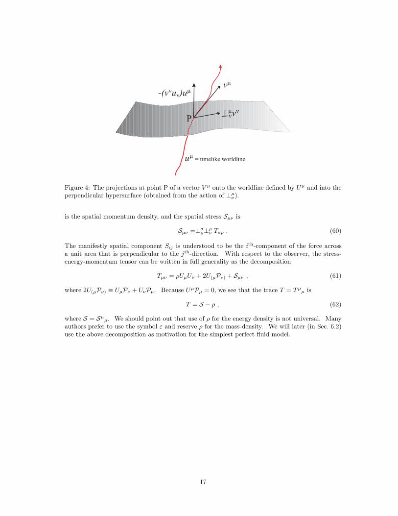
= timelike worldline
-(v u )unn
m
um
P
vm
m nvn
Figure 4: The projections at point P of a vector V µ onto the worldline defined by Uµ and into theperpendicular hypersurface (obtained from the action of ⊥µ
ν ).
is the spatial momentum density, and the spatial stress Sµν is
Sµν =⊥σµ⊥ρ
ν Tσρ . (60)
The manifestly spatial component Sij is understood to be the ith-component of the force acrossa unit area that is perpendicular to the jth-direction. With respect to the observer, the stress-energy-momentum tensor can be written in full generality as the decomposition
Tµν = ρUµUν + 2U(µPν) + Sµν , (61)
where 2U(µPν) ≡ UµPν + UνPµ. Because UµPµ = 0, we see that the trace T = T µµ is
T = S − ρ , (62)
where S = Sµµ. We should point out that use of ρ for the energy density is not universal. Many
authors prefer to use the symbol ε and reserve ρ for the mass-density. We will later (in Sec. 6.2)use the above decomposition as motivation for the simplest perfect fluid model.
17

4 Why are fluids useful models?
The Merriam-Webster online dictionary (http://www.m-w.com/) defines a fluid as “. . .a substance(as a liquid or gas) tending to flow or conform to the outline of its container” when taken as a nounand “. . .having particles that easily move and change their relative position without a separation ofthe mass and that easily yield to pressure: capable of flowing” when taken as an adjective. The bestmodel of physics is the Standard Model which is ultimately the description of the “substance” thatwill make up our fluids. The substance of the Standard Model consists of remarkably few classes ofelementary particles: leptons, quarks, and so-called “force” carriers (gauge-vector bosons). Eachelementary particle is quantum mechanical, but the Einstein equations require explicit trajectories.Moreover, cosmology and neutron stars are basically many particle systems and, even forgettingabout quantum mechanics, it is not practical to track each and every “particle” that makes themup. Regardless of whether these are elementary (leptons, quarks, etc) or collections of elementaryparticles (eg. stars in galaxies and galaxies in cosmology). The fluid model is such that the inherentquantum mechanical behaviour, and the existence of many particles are averaged over in such away that it can be implemented consistently in the Einstein equations.
Central to the model is the notion of “fluid particle,” also known as a fluid element. It isan imaginary, local “box” that is infinitesimal with respect to the system en masse and yet largeenough to contain a large number of particles (eg. an Avogadro’s number of particles). This isillustrated in Fig. 5. In order for the fluid model to work we require M >> N >> 1 and D >> L.Strictly speaking, our model has L infinitesimal, M → ∞, but with the total number of particlesremaining finite. The explicit trajectories that enter the Einstein equations are those of the fluidelements, not the much smaller (generally fundamental) particles that are “confined,” on average,to the elements. Hence, when we speak later of the fluid velocity, we mean the velocity of fluidelements.
DD
LL
N particles
M fluid elements
Figure 5: An object with a characteristic size D is modelled as a fluid that contains M fluidelements. From inside the object we magnify a generic fluid element of characteristic size L. Inorder for the fluid model to work we require M >> N >> 1 and D >> L.
In this sense, the use of the phrase “fluid particle” is very apt. For instance, each fluid elementwill trace out a timelike trajectory in spacetime. This is illustrated in Fig. 7 for a number of fluidelements. An object like a neutron star is a collection of worldlines that fill out continuously aportion of spacetime. In fact, we will see later that the relativistic Euler equation is little morethan an “integrability” condition that guarantees that this filling (or fibration) of spacetime can be
18

performed. The dual picture to this is to consider the family of three-dimensional hypersurfacesthat are pierced by the worldlines at given instants of time, as illustrated in Fig. 7. The integrabilitycondition in this case will guarantee that the family of hypersurfaces continuously fill out a portionof spacetime. In this view, a fluid is a so-called three-brane (see [18] for a general discussion ofbranes). In fact the method used in Sec. 8 to derive the relativistic fluid equations is based onthinking of a fluid as living in a three-dimensional “matter” space (i.e. the left-hand-side of Fig. 7).
Once one understands how to build a fluid model using the matter space, it is straight-forwardto extend the technique to single fluids with several constituents, as in Sec. 9, and multiple fluidsystems, as in Sec. 10. An example of the former would be a fluid with one species of particlesat a non-zero temperature, i.e. non-zero entropy, that does not allow for heat conduction relativeto the particles. (Of course, entropy does flow through spacetime.) The latter example canbe obtained by relaxing the constraint of no heat conduction. In this case the particles andthe entropy are both considered to be fluids that are dynamically independent, meaning that theentropy will have a four-velocity that is generally different from that of the particles. There isthus an associated collection of fluid elements for the particles and another for the entropy. Ateach point of spacetime that the system occupies there will be two fluid elements, in other words,there are two matter spaces (cf. Sec. 10). Perhaps the most important consequence of this is thatthere can be a relative flow of the entropy with respect to the particles (which in general leads tothe so-called entrainment effect). The canonical example of such a two fluid model is superfluidHe4 [89].
19

5 A Primer on Thermodynamics and Equations of State
Fluids consist of many fluid elements, and each fluid element consists of many particles. Thestate of matter in a given fluid element is determined thermodynamically [91], meaning that onlya few parameters are tracked as the fluid element evolves. Generally, not all the thermodynamicvariables are independent, being connected through the so-called equation of state. The numberof independent variables can also be reduced if the system has an overall additivity property. Asthis is a very instructive example, we will now illustrate such additivity in detail.
5.1 Fundamental, or Euler, Relation
Consider the standard form of the combined first and second laws for a simple, single-speciessystem:
dE = TdS − pdV + µdN . (63)
This follows because there is an equation of state, meaning that E = E(S, V, N) where
T =∂E
∂S
∣
∣
∣
∣
V,N
, p = − ∂E
∂V
∣
∣
∣
∣
S,N
, µ =∂E
∂N
∣
∣
∣
∣
S,V
. (64)
The total energy E, entropy S, volume V , and particle number N are said to be extensive if whenS, V , and N are doubled, say, then E will also double. Conversely, the temperature T , pressurep, and chemical potential µ are called intensive if they do not change their values when V , N , andS are doubled. This is the additivity property and we will now show that it implies an Eulerrelation (also known as the “fundamental relation” [91]) among the thermodynamic variables.
Let a tilde represent the change in thermodynamic variables when S, V , and N are all increasedby the same amount λ, i.e.
S = λS , V = λV , N = λN . (65)
Taking E to be extensive then means
E(S, V , N) = λE(S, V, N) . (66)
Of course we have for the intensive variables
T = T , p = p , µ = µ . (67)
Now,
dE = λdE + Edλ= TdS − pdV + µdN= λ (TdS − pdV + µdN) + (TS − pV + µN) dλ , (68)
and therefore we find the Euler relation
E = TS − pV + µN . (69)
If we let ρ = E/V denote the total energy density, s = S/V the total entropy density, and n = N/Vthe total particle number density, then
p + ρ = Ts + µn . (70)
The nicest feature of an extensive system is that the number of parameters required for acomplete specification of the thermodynamic state can be reduced by one, and in such a way thatonly intensive thermodynamic variables remain. To see this, let λ = 1/V , in which case
S = s , V = 1 , N = n . (71)
20

The re-scaled energy becomes just the total energy density, i.e. E = E/V = ρ, and moreoverρ = ρ(s, n) since
ρ = E(S, V , N) = E(S/V, 1, N/V ) = E(s, n) . (72)
The first law thus becomes
dE = TdS − pdV + µdN = Tds + µdn , (73)
ordρ = Tds + µdn . (74)
This implies
T =∂ρ
∂s
∣
∣
∣
∣
n
, µ =∂ρ
∂n
∣
∣
∣
∣
s
. (75)
The Euler relation Eq. (70) then yields the pressure as
p = −ρ + s∂ρ
∂s
∣
∣
∣
∣
n
+ n∂ρ
∂n
∣
∣
∣
∣
s
. (76)
We can think of a given relation ρ(s, n) as the equation of state, to be determined in the flat,tangent space at each point of the manifold, or, physically, a small enough region across which thechanges in the gravitational field are negligible, but also large enough to contain a large number ofparticles. For example, for a neutron star Glendenning [45] has reasoned that the relative changein the metric over the size of a nucleon with respect to the change over the entire star is about10−19, and thus one must consider many internucleon spacings before a substantial change in themetric occurs. In other words, it is sufficient to determine the properties of matter in specialrelativity, neglecting effects due to spacetime curvature. The equation of state is the major linkbetween the microphysics that governs the local fluid behaviour and global quantities (such as themass and radius of a star).
In what follows we will use a thermodynamic formulation that satisfies the fundamental scalingrelation, meaning that the local thermodynamic state (modulo entrainment) is a function of thevariables N/V , S/V , etcetera. This is in contrast to the fluid formulation of “MTW” [75]. Intheir approach one fixes from the outset the total number of particles N , meaning that one simplysets dN = 0 in the first law of thermodynamics. Thus without imposing any scaling relation, onecan write
dρ = d (E/V ) = Tds +1
n(p + ρ − T s) dn . (77)
This is consistent with our starting point for fluids, because we assume that the extensive variablesassociated with a fluid element do not change as the fluid element moves through spacetime.However, we feel that the use of scaling is necessary in that the fully conservative, or non-dissipative,fluid formalism presented below can be adapted to non-conservative, or dissipative, situations wheredN = 0 cannot be imposed.
5.2 From Microscopic Models to Fluid Equation of State
Let us now briefly discuss how an equation of state is constructed. For simplicity, we focus on a one-parameter system, with that parameter being the particle number density. The equation of statewill then be of the form ρ = ρ(n). In many-body physics (such as studied in condensed matter,nuclear, and particle physics) one can in principle construct the quantum mechanical particlenumber density nQM, stress-energy-momentum tensor T QM
µν , and associated conserved particlenumber density current nµ
QM (starting with some fundamental Lagrangian, say; cf. [109, 45, 110]).But unlike in quantum field theory in curved spacetime [12], one assumes that the matter exists
21

in an infinite Minkowski spacetime (cf. the discussion following Eq. (76)). If the reader likes, theapplication of T QM
µν at a spacetime point means that T QMµν has been determined with respect to a
flat tangent space at that point.Once T QM
µν is obtained, and after (quantum mechanical and statistical) expectation values withrespect to the system’s (quantum and statistical) states are taken, one defines the energy densityas
ρ = uµuν〈T QMµν 〉 , (78)
where
uµ ≡ 1
n〈nµ
QM〉 , n = 〈nQM〉 . (79)
At sufficiently small temperatures, ρ will just be a function of the number density of particles n atthe spacetime point in question, i.e. ρ = ρ(n). Similarly, the pressure is obtained as
p =1
3
(
〈T QMµµ〉 + ρ
)
(80)
and it will also be a function of n.One must be very careful to distinguish T QM
µν from Tµν . The former describes the states ofelementary particles with respect to a fluid element, whereas the latter describes the states of fluidelements with respect to the system. Comer and Joynt [32] have shown how this line of reasoningapplies to the two-fluid case.
22

6 An Overview of the Perfect Fluid
There are many different ways of constructing general relativistic fluid equations. Our purposehere is not to review all possible methods, but rather to focus on a couple: (i) an “off-the-shelve”consistency analysis for the simplest fluid a la Eckart [36], to establish some key ideas, and then (ii) amore powerful method based on an action principle that varies fluid element world lines. The ideasbehind this variational approach can be traced back to Taub [102] (see also [95]). Our descriptionof the method relies heavily on the work of Brandon Carter, his students, and collaborators [16, 33,34, 25, 26, 63, 85, 86]. We prefer this approach as it utilizes as much as possible the tools of thetrade of relativistic fields, i.e. no special tricks or devices will be required (unlike even in the case ofour “off-the-shelve” approach). One’s footing is then always made sure by well-grounded, action-based derivations. As Carter has always made clear: when there are multiple fluids, of both thecharged and uncharged variety, it is essential to distinguish the fluid momenta from the velocities.In particular, in order to make the geometrical and physical content of the equations transparent.A well-posed action is, of course, perfect for systematically constructing the momenta.
6.1 Rates-of-Change and Eulerian Versus Lagrangian Observers
The key geometric difference between generally covariant Newtonian fluids and their general rel-ativistic counterparts is that the former have an a priori notion of time [19, 20, 21]. Newtonianfluids also have an a priori notion of space (which can be seen explicitly in the Newtonian covariantderivative introduced earlier; cf. the discussion in [19]). Such a structure has clear advantages forevolution problems, where one needs to be unambiguous about the rate-of-change of the system.But once a problem requires, say, electromagnetism, then the a priori Newtonian time is at oddswith the full spacetime covariance of electromagnetic fields. Fortunately, for spacetime covarianttheories there is the so-called “3+1” formalism (see, for instance, [99]) that allows one to define“rates-of-change” in an unambiguous manner, by introducing a family of spacelike hypersurfaces(the “3”) given as the level surfaces of a spacetime scalar (the “1”).
Something that Newtonian and relativistic fluids have in common is that there are preferredframes for measuring changes—those that are attached to the fluid elements. In the parlanceof hydrodynamics, one refers to Lagrangian and Eulerian frames, or observers. A NewtonianEulerian observer is one who sits at a fixed point in space, and watches fluid elements pass by,all the while taking measurements of their densities, velocities, etc. at the given location. Incontrast, a Lagrangian observer rides along with a particular fluid element and records changes ofthat element as it moves through space and time. A relativistic Lagrangian observer is the same,but the relativistic Eulerian observer is more complicated to define. Smarr and York [99] definesuch an observer as one who would follow along a worldline that remains everywhere orthogonalto the family of spacelike hypersurfaces.
The existence of a preferred frame for a one fluid system can be used to great advantage. Inthe very next sub-section we will use an “off-the-shelve” analysis that exploits the fact of onepreferred frame to derive the standard perfect fluid equations. Later, we will use Eulerian andLagrangian variations to build an action principle for the single and multiple fluid systems. Thesesame variations can also be used as the foundation for a linearized perturbation analysis of neutronstars [59]. As we will see, the use of Lagrangian variations is absolutely essential for establishinginstabilities in rotating fluids [41, 42]. Finally, we point out that multiple fluid systems can haveas many notions of Lagrangian observer as there are fluids in the system.
23

6.2 The Single, Perfect Fluid Problem: “Off-the-shelve” Consistency
Analysis
We earlier took the components of a general stress-energy-momentum tensor and projected themonto the axes of a coordinate system carried by an observer moving with four-velocity Uµ. Asmentioned above, the simplest fluid is one for which there is only one four-velocity uµ. Hence,there is a preferred frame defined by uµ and if we want the observer to sit in this frame we cansimply take Uµ = uµ. With respect to the fluid there will be no momentum flux, i.e. Pµ = 0. Sincewe use a fully spacetime covariant formulation, i.e. there are only spacetime indices, the resultingstress-energy-momentum tensor will transform properly under general coordinate transformations,and hence can be used for any observer.
The spatial stress is a two-index, symmetric tensor, and the only objects that can be used tocarry the indices are the four-velocity uµ and the metric gµν . Furthermore, because the spatialstress must also be symmetric, the only possibility is a linear combination of gµν and uµuν . Giventhat uµSµν = 0, we find
Sµν =1
3S(gµν + uµuν) . (81)
If we identify the pressure as p = S/3 [36], then
Tµν = (ρ + p)uµuν + pgµν , (82)
which is the well-established result for a perfect fluid.Given a relation p = p(ρ), there are four independent fluid variables. Because of this the
equations of motion are often understood to be ∇µT µν = 0, which follows immediately from the
Einstein equations and the fact that ∇µGµν = 0. To simplify matters, we take as equation of state
a relation of the form ρ = ρ(n) where n is the particle number density. The chemical potential isthen given by
dρ =∂ρ
∂ndn ≡ µdn , (83)
and we see from the Euler relation Eq. (70) that
µn = p + ρ . (84)
Let us now get rid of the free index of ∇µT µν = 0 in two ways: first, by contracting it with uν
and second, by projecting it with ⊥νρ (letting Uµ = uµ). Recalling the fact that uµuµ = −1 we
have the identity∇µ (uνuν) = 0 ⇒ uν∇µuν = 0 . (85)
Contracting with uν and using this identity gives
uµ∇µρ + (ρ + p)∇µuµ = 0 . (86)
The definition of the chemical potential µ and the Euler relation allow us to rewrite this as
µuµ∇µn + µn∇µuµ ⇒ ∇µnµ = 0 , (87)
where nµ ≡ nuµ. Projection of the free index using ⊥ρµ leads to
Dµp = −(ρ + p)aµ , (88)
where Dµ ≡⊥ρµ ∇ρ is a purely spatial derivative and aµ ≡ uν∇νuµ is the acceleration. This is
reminiscent of the familiar Euler equation for Newtonian fluids.
24

However, we should not be too quick to think that this is the only way to understand ∇µT µν =
0. There is an alternative form that makes the perfect fluid have much in common with vacuumelectromagnetism. If we define
µµ = µuµ , (89)
and note that uµduµ = 0 (because uµuµ = −1), then
dρ = −µµdnµ . (90)
The stress-energy-momentum tensor can now be written in the form
T µν = pδµ
ν + nµµν . (91)
We have here our first encounter with the momentum µµ that is conjugate to the particle numberdensity current nµ. Its importance will become clearer as this review develops, particularly whenwe discuss the two-fluid case. If we now project onto the free index of ∇µT µ
ν = 0 using ⊥µν , as
before, we findfν + (∇µnµ)µν = 0 , (92)
where the force density fν isfν = 2nµωµν , (93)
and the vorticity ωµν is defined as
ωµν ≡ ∇[µµν] =1
2(∇µµν −∇νµµ) . (94)
Contracting Eq. (92) with nν implies (since ωµν = −ωνµ) that
∇µnµ = 0 (95)
and as a consequencefν = 2nµωµν = 0 . (96)
The vorticity two-form ωµν has emerged quite naturally as an essential ingredient of the fluiddynamics [67, 16, 10, 57]. Those who are familiar with Newtonian fluids should be inspiredby this, as the vorticity is often used to establish theorems on fluid behaviour (for instance theKelvin-Helmholtz Theorem [62]) and is at the heart of turbulence modelling [88].
To demonstrate the role of ωµν as the vorticity, consider a small region of the fluid where thetime direction tµ, in local Cartesian coordinates, is adjusted to be the same as that of the fluidfour-velocity so that uµ = tµ = (1, 0, 0, 0). Eq. (96) and the antisymmetry then imply that ωµν
can only have purely spatial components. Because the rank of ωµν is two, there are two “nulling”vectors, meaning their contraction with either index of ωµν yields zero (a condition which is truealso of vacuum electromagnetism). We have arranged already that tµ be one such vector. Bya suitable rotation of the coordinate system the other one can be taken as zµ = (0, 0, 0, 1), thusimplying that the only non-zero component of ωµν is ωxy. “MTW” [75] points out that such atwo-form can be pictured geometrically as a collection of oriented worldtubes, whose walls lie in thex = constant and y = constant planes. Any contraction of a vector with a two-form that does notyield zero implies that the vector pierces the walls of the worldtubes. But when the contraction iszero, as in Eq. (96), the vector does not pierce the walls. This is illustrated in Fig. 6, where the redcircles indicate the orientation of each world-tube. The individual fluid element four-velocities liein the centers of the world-tubes. Finally, consider the dashed, closed contour in Fig. 6. If thatcontour is attached to fluid-element worldlines, then the number of worldtubes contained withinthe contour will not change because the worldlines cannot pierce the walls of the worldtubes. This
25

x
yt
Figure 6: A local, geometrical view of the Euler equation as an integrability condition of thevorticity for a single-constituent perfect fluid.
is essentially the Kelvin-Helmholtz Theorem on conservation of vorticity. From this we learn thatthe Euler equation is an integrability condition which ensures that the vorticity two-surfaces meshtogether to fill out spacetime.
As we have just seen, the form Eq. (96) of the equations of motion can be used to discuss theconservation of vorticity in an elegant way. It can also be used as the basis for a derivation ofother known theorems in fluid mechanics. To illustrate this, let us derive a generalized form ofBernoulli’s theorem. Let us assume that the flow is invariant with respect to transport by somevector field kρ. That is, we have
Lkµρ = 0 , −→ (∇ρµσ −∇σµρ)kσ = ∇ρ(k
σµσ) . (97)
Here one may consider two particular situations. If kσ is taken to be the four-velocity, then thescalar kσµσ represents the “energy per particle”. If instead kσ represents an axial generator ofrotation, then the scalar will correspond to an angular momentum. For the purposes of the presentdiscussion we can leave kσ unspecified, but it is still useful to keep these possibilities in mind. Nowcontract the equation of motion Eq. (96) with kσ and assume that the conservation law Eq. (95)holds. Then it is easy to show that we have
nρ∇ρ (µσkσ) = ∇ρ (nρµσkσ) = 0 . (98)
In other words, we have shown that nρµσkσ is a conserved quantity.Given that we have just inferred the equations of motion from the identity that ∇µT µ
ν = 0, wenow emphatically state that while the equations are correct the reasoning is severely limited. Infact, from a field theory point of view it is completely wrong! The proper way to think about theidentity is that the equations of motion are satisfied first, which then guarantees that ∇µT µ
ν = 0.There is no clearer way to understand this than to study the multi-fluid case: Then the vanishingof the covariant divergence represents only four equations, whereas the multi-fluid problem clearlyrequires more information (as there are more velocities that must be determined). We havereached the end of the road as far as the “off-the-shelf” strategy is concerned, and now move onto an action-based derivation of the fluid equations of motion.
26

7 Setting the Context: The Point Particle
The simplest physics problem, i.e. the point particle, has always served as a guide to deep principlesthat are used in much harder problems. We have used it already to motivate parallel transportas the foundation for the covariant derivative. Let us call upon the point particle again to set thecontext for the action-based derivation of the fluid field equations. We will simplify the discussionby considering only motion in one dimension. We assure the reader that we have good reasons,and ask for patience while we remind him/her of what may be very basic facts.
Early on we learn that an action appropriate for the point particle is
I =
∫ tf
ti
dt T =
∫ tf
ti
dt
(
1
2mx2
)
, (99)
where m is the mass and T the kinetic energy. A first-order variation of the action with respectto x(t) yields
δI = −∫ tf
ti
dt (mx) δx + (mxδx)|tf
ti. (100)
If this is all the physics to be incorporated, i.e. if there are no forces acting on the particle, thenwe impose d’Alembert’s principle of least action [61], which states that those trajectories x(t) thatmake the action stationary, i.e. δI = 0, are those that yield the true motion. We see from theabove that functions x(t) that satisfy the boundary conditions
δx(ti) = 0 = δx(tf ) , (101)
and the equation of motionmx = 0 , (102)
will indeed make δI = 0. This same reasoning applies in the substantially more difficult fluidactions that will be considered later.
But, of course, forces need to be included. First on the list are the so-called conservative forces,describable by a potential V (x), which are placed into the action according to:
I =
∫ tf
ti
dtL(x, x) =
∫ tf
ti
dt
(
1
2mx2 − V (x)
)
, (103)
where L = T − V is the so-called Lagrangian. The variation now leads to
δI = −∫ tf
ti
dt
(
mx +∂V
∂x
)
δx + (mxδx)|tf
ti. (104)
Assuming no externally applied forces, d’Alembert’s principle yields the equation of motion
mx +∂V
∂x= 0 . (105)
An alternative way to write this is to introduce the momentum p (not to be confused with thefluid pressure introduced earlier) defined as
p =∂L
∂x= mx , (106)
in which case
p +∂V
∂x= 0 . (107)
27

In the most honest applications, one has the obligation to incorporate dissipative, i.e. non-conservative, forces. Unfortunately, dissipative forces Fd cannot be put into action principles.Fortunately, Newton’s second law is of great guidance, since it states
mx +∂V
∂x= Fd , (108)
when conservative and dissipative forces act. A crucial observation of Eq. (108) is that the“kinetic” (mx = p) and conservative (∂V/∂x) forces, which enter the left-hand side, do follow fromthe action, i.e.
δI
δx= −
(
mx +∂V
∂x
)
. (109)
When there are no dissipative forces acting, the action principle gives us the appropriate equationof motion. When there are dissipative forces, the action defines for us the kinetic and conservativeforce terms that are to be balanced by the dissipative terms. It also defines for us the momentum.
We should emphasize that this way of using the action to define the kinetic and conservativepieces of the equation of motion, as well as the momentum, can also be used in a context where thesystem experiences an externally applied force Fext. The force can be conservative or dissipative,and will enter the equation of motion in the same way as Fd did above. That is
− δI
δx= Fd + Fext . (110)
Like a dissipative force, the main effect of the external force can be to siphon kinetic energy fromthe system. Of course, whether a force is considered to be external or not depends on the a prioridefinition of the system. To summarize: The variational argument leads to equations of motionof the form
− δI
δx= mx +
∂V
∂x= p +
∂V
∂x
= 0 Conservative6= 0 Dissipative and/or External Forces
(111)
28

8 The “Pull-back” Formalism for a Single Fluid
In this section the equations of motion and the stress-energy-momentum tensor for a one-component,general relativistic fluid are obtained from an action principle. Specifically a so-called “pull-back”approach (see, for instance, [33, 34, 31]) is used to construct a Lagrangian displacement of thenumber density four-current nµ, whose magnitude n is the particle number density. This willform the basis for the variations of the fundamental fluid variables in the action principle.
As there is only one species of particle considered here, nµ is conserved, meaning that once anumber of particles N is assigned to a particular fluid element, then that number is the same ateach point of the fluid element’s worldline. This would correspond to attaching a given numberof particles (i.e. N1, N2, etc.) to each of the worldlines in Fig. 7. Mathematically, one can writethis as a standard particle-flux conservation equation:
∇µnµ = 0 . (112)
For reasons that will become clear shortly, it is useful to rewrite this conservation law in what may(if taken out context) seem a rather obscure way. We introduce the dual nνλτ to nµ, i.e.
nνλτ = ǫνλτµnµ , nµ =1
3!ǫµνλτnνλτ , (113)
such that
n2 =1
3!nνλτnνλτ , (114)
In Fig. 6 we have seen that a two-form gives worldtubes. A three-form is the next higher-rankedobject and it can be thought of, in an analogous way, as leading to boxes [75]. The key step hereis to realize that the conservation rule is equivalent to having the three-form nνλτ be closed. Indifferential geometry this means that
∇[µnνλτ ] = 0 . (115)
This can be shown to be equal to Eq. (112) by contracting with ǫµνλτ .The main reason for introducing the dual is that it is straightforward to construct a particle
number density three-form that is automatically closed, since the conservation of the particlenumber density current should not—speaking from a strict field theory point of view—be a part ofthe equations of motion, but rather should be automatically satisfied when evaluated on a solutionof the “true” equations.
This can be made to happen by introducing a three-dimensional “matter” space—the left-handpart of Fig. 7—which can be labelled by coordinates XA = XA(xµ), where A, B, C etc = 1, 2, 3.For each time slice in spacetime, there will be a corresponding configuration in the matter space;that is, as time goes forward, the weaving of worldlines in spacetime will be matched by the fluidparticle positions in the matter space. In this sense we are “pulling-back” from spacetime to thematter space (cf. the previous discussion of the Lie derivative). The three-form can be pulled-backto its three-dimensional matter space by using the mappings XA, as indicated in Fig. 7. Thisallows us to construct a three-form that is automatically closed on spacetime. Hence, we let
nνλτ = NABC
(
∇νXA) (
∇λXB)
∇τXC , (116)
where NABC is completely antisymmetric in its indices and is a function only of the XA. The XA
will also be comoving in the sense that
nµ∇µXA =1
3!ǫµνλτNBCD
(
∇νXB) (
∇λXC) (
∇τXD)
∇µXA = 0 . (117)
29

X1
X2
t=0
1
2 3
4
N2
N1N3
N4
XA3
x1i
x2i
x3i
x4i
X3
Figure 7: The pull-back from “fluid-particle” worldlines in spacetime, on the right, to “fluid-particle” points in the three-dimensional matter space labelled by the coordinates X1, X2, X3.Here, the pull-back of the “Ith” (I = 1, 2, ..., n) worldline into the abstract space (for the t = 0configuration of “fluid-particle” points) is XA
I = XA(0, xiI) where xi
I is the spatial position of theintersection of the worldline with the t = 0 time slice.
The time part of the spacetime dependence of the XA is thus somewhat ad hoc; that is, if we wouldtake the flow of time to be the proper time of the worldlines, then the XA would not change, andhence there would be no “motion” of the fluid particles in the matter space.
Because the matter space indices are three-dimensional and the closure condition involves fourspacetime indices, and also the XA are scalars on spacetime (and thus two covariant differentiationscommute), the pull-back construction does indeed produce a closed three-form:
∇[µnνλτ ] = ∇[µ
(
NABC∇νXA∇λXB∇τ ]XC
)
≡ 0 . (118)
In terms of the scalar fields XA, we now have particle number density currents that are automati-cally conserved. Thus, another way of viewing the pull-back construction is that the fundamentalfluid field variables are the XA (as evaluated on spacetime). In fact, the variations of nνλτ cannow be taken with respect to variations of the XA.
Let us introduce the Lagrangian displacement on spacetime for the particles, to be denoted ξµ.This is related to the variation δXA via a “push-forward” construction (which takes a variation inthe matter space and pushes it forward to spacetime):
δXA = −(
∇µXA)
ξµ . (119)
Using the fact that
∇νδXA = −∇ν
([
∇µXA]
ξµ)
= −(
∇µXA)
∇νξµ −(
∇µ∇νXA)
ξµ (120)
means [63]
δnνλτ = − (ξσ∇σnνλτ + nσλτ∇νξσ + nνστ∇λξσ + nνλσ∇τ ξσ) = −Lξnνλτ , (121)
where L is the Lie derivative along ξµ (cf. Eq. (42)). We can thus infer that
δnµ = nσ∇σξµ − ξσ∇σnµ − nµ
(
∇σξσ +1
2gσρδgσρ
)
. (122)
30

By introducing the decomposition
nµ = nuµ , uµuµ = −1 , (123)
we can furthermore show that
δn = −∇σ (nξσ) − n
(
uνuσ∇σξν +1
2[gσρ + uσuρ] δgσρ
)
, (124)
and
δuµ =(
δµρ + uµuρ
)
(uσ∇σξρ − ξσ∇σuρ) +1
2uµuσuρδgσρ . (125)
The Lagrangian variation resulting from the Lagrangian displacement is given by
∆ ≡ δ + Lξ , (126)
from which it follows that∆nµλτ = 0 , (127)
which is entirely consistent with the pull-back construction. We also find that
∆uµ =1
2uµuσuρ∆gσρ , (128)
∆ǫνλτσ =1
2ǫνλτσgµρ∆gµρ , (129)
and∆n = −n
2(gσρ + uσuρ)∆gσρ . (130)
These formulae (and their Newtonian analogues) have been adroitly used by Friedman and Schutzin their establishment of the so-called Chandrasekhar-Friedman-Schutz (CFS) instability [27, 41,42], see Sec. 13.
With a general variation of the conserved four-current in hand, we can now use an actionprinciple to derive the equations of motion and the stress-energy-momentum tensor. The centralquantity in the analysis is the so-called “master” function Λ, which is a function of the scalar n2 =−nµnµ. For this single fluid system, it is such that −Λ corresponds to the local thermodynamicenergy density. In the action principle, the master function is the Lagrangian density for the fluid:
Ifluid =
∫
M
√−gΛd4x . (131)
An unconstrained variation of Λ(n2) is with respect to nµ and the metric gµν , and allows thefour components of nµ to be varied independently. It takes the form
δΛ = µµδnµ +1
2nµµνδgµν , (132)
where
µµ = Bnµ , B ≡ −2∂Λ
∂n2. (133)
The use of the letter B is to remind us that this is a bulk fluid effect, which is present regardlessof the number of fluids and constituents. The momentum covector µµ is what we encounteredearlier. It is dynamically, and thermodynamically, conjugate to nµ, and its magnitude can beseen to be the chemical potential of the particles by recalling that Λ = −ρ. Correctly identifyingthe momentum is essential for a concise and transparent formulation of fluids, e.g. for constructing
31
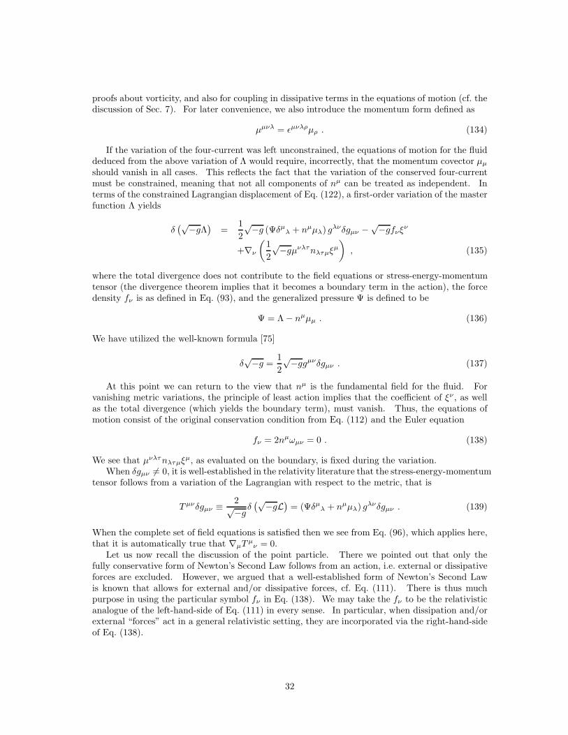
proofs about vorticity, and also for coupling in dissipative terms in the equations of motion (cf. thediscussion of Sec. 7). For later convenience, we also introduce the momentum form defined as
µµνλ = ǫµνλρµρ . (134)
If the variation of the four-current was left unconstrained, the equations of motion for the fluiddeduced from the above variation of Λ would require, incorrectly, that the momentum covector µµ
should vanish in all cases. This reflects the fact that the variation of the conserved four-currentmust be constrained, meaning that not all components of nµ can be treated as independent. Interms of the constrained Lagrangian displacement of Eq. (122), a first-order variation of the masterfunction Λ yields
δ(√−gΛ
)
=1
2
√−g (Ψδµλ + nµµλ) gλνδgµν −√−gfνξν
+∇ν
(
1
2
√−gµνλτnλτµξµ
)
, (135)
where the total divergence does not contribute to the field equations or stress-energy-momentumtensor (the divergence theorem implies that it becomes a boundary term in the action), the forcedensity fν is as defined in Eq. (93), and the generalized pressure Ψ is defined to be
Ψ = Λ − nµµµ . (136)
We have utilized the well-known formula [75]
δ√−g =
1
2
√−ggµνδgµν . (137)
At this point we can return to the view that nµ is the fundamental field for the fluid. Forvanishing metric variations, the principle of least action implies that the coefficient of ξν , as wellas the total divergence (which yields the boundary term), must vanish. Thus, the equations ofmotion consist of the original conservation condition from Eq. (112) and the Euler equation
fν = 2nµωµν = 0 . (138)
We see that µνλτnλτµξµ, as evaluated on the boundary, is fixed during the variation.When δgµν 6= 0, it is well-established in the relativity literature that the stress-energy-momentum
tensor follows from a variation of the Lagrangian with respect to the metric, that is
T µνδgµν ≡ 2√−gδ(√−gL
)
= (Ψδµλ + nµµλ) gλνδgµν . (139)
When the complete set of field equations is satisfied then we see from Eq. (96), which applies here,that it is automatically true that ∇µT µ
ν = 0.Let us now recall the discussion of the point particle. There we pointed out that only the
fully conservative form of Newton’s Second Law follows from an action, i.e. external or dissipativeforces are excluded. However, we argued that a well-established form of Newton’s Second Lawis known that allows for external and/or dissipative forces, cf. Eq. (111). There is thus muchpurpose in using the particular symbol fν in Eq. (138). We may take the fν to be the relativisticanalogue of the left-hand-side of Eq. (111) in every sense. In particular, when dissipation and/orexternal “forces” act in a general relativistic setting, they are incorporated via the right-hand-sideof Eq. (138).
32
9 The Two-Constituent, Single Fluid
Generally speaking, the total energy density ρ can be a function of independent parameters otherthan the particle number density nn, such as the entropy density ns, assuming that the systemscales in the manner discussed in Sec. 5 so that only densities need enter the equation of state.(For later convenience we will introduce the constituent indices x, y, etc., which range over thetwo constituents n, s, and do not satisfy any kind of summation convention.) If there is noheat conduction, then this is still a single fluid problem, meaning that there is still just one unitflow velocity uµ [33]. This is what we mean by a two-constituent, single fluid. We assumethat the particle number and entropy are both conserved along the flow, in the same sense as inEq. (117). Associated which each parameter there is thus a conserved current density four-vector,i.e. nµ
n = nnuµ for the particle number density and nµs = nsu
µ for the entropy density. Note thatthe ratio xs = ns/nn is comoving in the sense that
uµ∇µ (xs) = 0 . (140)
In terms of constituent indices x, y, the associated first law can be written in the form
dρ =∑
x=n,s
µxdnx = −∑
x=n,s
µxµdnµ
x , (141)
since ρ = ρ(n2n, n2
s ), wherenµ
x = nxuµ , n2
x = −gµνnµxnν
x , (142)
and
µxµ = gµνBxnν
x , Bx ≡ 2∂ρ
∂n2x
. (143)
Because of Eq. (74) µs = T where T is the temperature.Given that we only have one four-velocity, the system will still just have one fluid element per
spacetime point. But unlike before, there will be an additional conserved number, Ns, that canbe attached to each worldline, like the particle number Nn of Fig. 7. In order to describe theworldlines we can use the same three scalars XA(xµ) as before. But how do we get a constructionthat allows for the additional conserved number? Recall that the intersections of the worldlineswith some hypersurface, say t = 0, is uniquely specified by the three XA(0, xi) scalars. Eachworldline will have also the conserved numbers Nn and Ns assigned to them. Thus, the valuesof these numbers can be expressed as functions of the XA(0, xi). But most importantly, the factthat each Nx is conserved, means that this function specification must hold for all of spacetime,so that in particular the ratio xs is of the form xs(x
µ) = xs(XA(xµ)). Consequently, we now have
a construction whereby this ratio identically satisfies Eq. (140), and the action principle remainsa variational problem just in terms of the three XA scalars.
The variation of the action follows like before, except now a constituent index x must beattached to the particle number density current and three-form:
nxνλτ = ǫνλτµnµ
x . (144)
Once again it is convenient to introduce the momentum form, now defined as
µµνλx = ǫµνλρµx
ρ . (145)
Since the XA are the same for each nxνλτ , the above discussion indicates that the pull-back con-
struction now is to be based on
nxνλτ = Nx
ABC
(
∇νXA) (
∇λXB)
∇τXC , (146)
33

where NxABC is completely antisymmetric and a function of the XA. After some due deliberation,
the reader should be convinced that the only thing required here in addition to the previoussubsection is to attach a x index to nνλτ , nµ, and n in Eqs. (121), (122), and (124), respectively.If we now define the master function as
Λ = −ρ (147)
and the generalized pressure Ψ to be
Ψ = Λ −∑
x=n,s
µxµnµ
x = Λ +∑
x=n,s
µxnx , (148)
then the first-order variation for Λ is
δ(√−gΛ
)
=1
2
√−g (Ψgµν + [Ψ − Λ] uµuν) δgµν −√−g
∑
x=n,s
fxν
ξν+
∇ν
1
2
√−g∑
x=n,s
µνλτx nx
λτµξµ
, (149)
wherefx
ν = 2nµxωx
µν , (150)
andωx
µν = ∇[µµxν] . (151)
The final equations of motion are∑
x=n,s
fxν = 0 , (152)
and∇νnν
x = 0 , (153)
whereas the stress-energy-momentum tensor takes the familiar form
T µν = Ψgµν + (Ψ − Λ)uµuν . (154)
34

10 The “Pull-Back” Formalism for Two Fluids
Having discussed the single fluid model, and how one accounts for stratification, it is time tomove on to the problem of modelling multi-fluid systems. We will experience for the first timenovel effects due to the presence of a relative flow between two, interpenetrating fluids, and thefact that there is no longer a single, preferred rest-frame. This kind of formalism is necessary,for example, for the simplest model of a neutron star, since it is generally accepted that theinner crust is permeated by an independent neutron superfluid, and the outer core is thought tocontain superfluid neutrons, superconducting protons, and a highly degenerate gas of electrons.Still unknown is the number of independent fluids that would be required for neutron stars thathave colour-flavour-locked quark matter in the deep core [1]. The model can also be used todescribe superfluid Helium and heat-conducting fluids, which is of importance for incorporationof dissipation (see Sec. 14). We will focus on this example here. It should be noted that, eventhough the particular system we concentrate on consists of only two fluids it illustrates all newfeatures of a general multi-fluid system. Conceptually, the greatest step is to go from one to twofluids. A generalization to a system with more degrees of freedoms is straightforward.
In keeping with the previous section, we will rely on use of the constituent index, which for allremaining formulas of this section will range over x, y, z = n, s. In the example that we considerthe two fluids represent the particles (n) and the entropy (s). Once again, the number densityfour-currents, to be denoted nµ
x , are taken to be separately conserved, meaning
∇µnµx = 0 . (155)
As before, we use the dual formulation, i.e. introduce the three-forms
nxνλτ = ǫνλτµnµ
x , nµx =
1
3!ǫµνλτnx
νλτ . (156)
Also like before, the conservation rules are equivalent to the individual three-forms being closed,i.e.
∇[µnxνλτ ] = 0 . (157)
However, we need a formulation whereby such conservation obtains automatically, at least inprinciple.
We make this happen by introducing the three-dimensional matter space, the difference beingthat we now need two such spaces. These will be labelled by coordinates XA
x , and we recall thatA, B, C etc = 1, 2, 3. This is depicted in Fig. 8, which indicates the important facts that (i) agiven spatial point can be intersected by each fluid’s worldline and (ii) the individual worldlinesare not necessarily parallel at the intersection, i.e. the independent fluids are interpenetrating andcan exhibit a relative flow with respect to each other. Although we have not indicated this inFig. 8 (in order to keep the figure as uncluttered as possible) attached to each worldline of a givenconstituent will be a fixed number of particles Nx
1 , Nx2 , etc. (cf. Fig. 7). For the same reason, we
have also not labelled (as in Fig. 7) the “pull-backs” (represented by the arrows) from spacetimeto the matter spaces.
By “pulling-back” each constituent’s three-form onto its respective matter space we can onceagain construct three-forms that are automatically closed on spacetime, i.e. let
nxνλτ = Nx
ABC∇νXAx ∇λXB
x ∇τXCx , (158)
where NxABC is completely antisymmetric in its indices and is a function of the XA
x . Using thesame reasoning as in the single fluid case, the pull-back construction produces three-forms thatare automatically closed, i.e. they satisfy Eq. (157) identically. If we let the scalar fields XA
x (asfunctions on spacetime) be the fundamental variables, they yield a representation for each particle
35

t=0x1
i x2i
x3i
x4i
X1
X2
1
2 3
4
X3
X1
X2
1
2
3
4
X3
2
2
2
1
1
1
Figure 8: The pull-back from an xth-constituent “fluid-particle” worldline in spacetime, on theright, to “fluid-particle” points in that xth-constituent’s three-dimensional matter space labelledby the coordinates X1
x , X2x , X3
x, where the constituent index x = n, s. There exist as manymatter spaces as there are dynamically independent fluids, which for this case means two.
number density current that is automatically conserved. The variations of the three-forms cannow be derived by varying them with respect to the XA
x .Lagrangian displacements on spacetime for each fluid, to be denoted ξµ
x , will now be introduced.They are related to the variations δXA
x via the “push-forwards”
δXAx = −
(
∇µXAx
)
ξµx . (159)
It should be clear that the analogues of Eqs. (121), (122), (124), and (125) for this two-fluid case aregiven by the same formulas except that each displacement and four-current will now be associatedwith a constituent index, using the decomposition
nµx = nxu
µx , ux
µuµx = −1 , (160)
where uxµ = gµνuν
x.Associated with each constituent’s Lagrangian displacement is its own Lagrangian variation.
These are naturally defined to be∆x ≡ δ + Lξx
, (161)
so that it follows that∆xn
xµλτ = 0 , (162)
as expected for the pull-back construction. Likewise, two-fluid analogues of Eqs. (128)–(130) existwhich take the same form except that the constituent index is attached. However, in contrastto the ordinary fluid case, there are many more options to consider. For instance, we could alsolook at the Lagrangian variation of the first constituent with respect to the second constituent’sflow, i.e. ∆snn, or the other way around, i.e. ∆nns. The Newtonian analogues of these Lagrangiandisplacements were essential to an analysis of instabilities in rotating superfluid neutron stars [7].
36
We are now in a position to construct an action principle that will yield the equations of motionand the stress-energy tensor. Again, the central quantity is the “master” function Λ, which is nowa function of all the different scalars that can be formed from the nµ
x , i.e. the scalars nx togetherwith
n2xy = n2
yx = −gµνnµxnν
y . (163)
In the limit where all the currents are parallel, i.e. the fluids are comoving, −Λ corresponds againto the local thermodynamic energy density. In the action principle, Λ is the Lagrangian density forthe fluids. It should be noted that our choice to use only the fluid currents to form scalars impliesthat the system is “locally isotropic” in the sense that there are no a priori preferred directions,i.e. the fluids are equally free to move in any direction. Structures like the crust believed to existnear the surface of a neutron star generally would be locally anisotropic, eg. sound waves in thelattice move in the preferred directions associated with the lattice.
An unconstrained variation of Λ with respect to the independent vectors nµx and the metric gµν
takes the form
δΛ =∑
x=n,s
µxµδnµ
x +1
2gλν
∑
x=n,s
nµxµx
λ
δgµν , (164)
whereµx
µ = gµν
(
Bxnνx + Axynν
y
)
, (165)
Axy = Ayx = − ∂Λ
∂n2xy
, x 6= y . (166)
The momentum covectors µxµ are each dynamically, and thermodynamically, conjugate to their
respective number density currents nµx , and their magnitudes are the chemical potentials. We see
that Axy represents the fact that each fluid momentum µxµ may, in general, be given by a linear
combination of the individual currents nµx . That is, the current and momentum for a particular
fluid do not have to be parallel. This is known as the entrainment effect. We have chosen torepresent it by the letter A for historical reasons. When Carter first developed his formalism heopted for this notation, referring to the “anomaly” of having misaligned currents and momenta.It has since been realized that the entrainment is a key feature of most multi-fluid systems and itwould, in fact, be anomalous to leave it out!
In the general case, the momentum of one constituent carries along some mass current of theother constituents. The entrainment only vanishes in the special case where Λ is independentof n2
xy (x 6= y) because then we obviously have Axy = 0. Entrainment is an observable effectin laboratory superfluids [89, 104] (eg. via flow modifications in superfluid 4He and mixtures ofsuperfluid 3He and 4He). In the case of neutron stars, entrainment is an essential ingredient ofthe current best explanation for the so-called glitches [90, 92]. Carter [16] has also argued thatthese “anomalous” terms are necessary for causally well-behaved heat conduction in relativisticfluids, and by extension necessary for building well-behaved relativistic equations that incorporatedissipation.
In terms of the constrained Lagrangian displacements, a variation of Λ now yields
δ(√
−gΛ)
=1
2
√−g
Ψδµλ +
∑
x=n,s
nµxµx
λ
gλνδgµν −√−g
∑
x=n,s
fxν ξν
x
+∇ν
1
2
√−g∑
x=n,s
µνλτx nx
λτµξµx
, (167)
37

where fxν is as defined in Eq. (150) except that the individual velocities are no longer parallel. The
generalized pressure Ψ is now
Ψ = Λ −∑
x=n,s
nµxµx
µ . (168)
At this point we will return to the view that nµn and nµ
s are the fundamental variables for thefluids. Because the ξµ
x are independent variations, the equations of motion consist of the twooriginal conservation conditions of Eq. (155) plus two Euler type equations
fxν = 0 . (169)
We also find that the stress-energy tensor is
T µν = Ψδµ
ν +∑
x=n,s
nµxµx
ν . (170)
When the complete set of field equations is satisfied then it is automatically true that ∇µT µν = 0.
One can also verify that Tµν is symmetric. The momentum form µµνλx entering the boundary
term is the natural extension of Eq. (145) to this two-fluid case.It must be noted that Eq. (169) is significantly different from the multi-constituent version of
Eq. (152). This is true even if one is solving for a static and spherically symmetric configura-tion, where the fluid four-velocities would all necessarily be parallel. Simply put, Eq. (169) stillrepresents two independent equations. If one takes entropy as an independent fluid, then thestatic and spherically symmetric solutions will exhibit thermal equilibrium [35]. This explains,for instance, why one must specify an extra condition (eg. convective stability [111]) to solve for adouble-constituent star with only one four-velocity.
38

11 Speeds of Sound
Crucial to the understanding of black holes is the effect of spacetime curvature on the light-conestructures, that is, the totality of null vectors that emanate from each spacetime point. Crucialto the propagation of massless fields is the light-cone structure. In the case of fluids, it is both thespeed of light and the speed (and/or speeds) of sound that dictate how waves propagate throughthe matter, and thus how the matter itself propagates. We give here a simple analysis that usesplane-wave propagation to derive the speed(s) of sound in the single-fluid, two-constituent single-fluid, and two-fluid cases, assuming that the metric variations vanish (see [16] for a more rigorousderivation). The analysis is local, assuming that the speed of sound is a locally defined quantity,and performed using local, Minkowski coordinates xµ. The purpose of the analysis is to illuminatehow the presence of various constituents and multi-fluids impact the local dynamics.
In a small region we will assume that the configuration of the matter with no waves presentis locally isotropic, homogeneous, and static. Thus for the background nµ
x = nx, 0, 0, 0 and thevorticity ωx
µν vanishes. For all cases the general form of the variation of the force density fxν for
each constituent isδfx
ν = 2nµx∂[µδµx
ν] . (171)
Similarly, the conservation of the nµx gives
∂µδnµx = 0 . (172)
We are here using the point of view that the nµx are the fundamental fluid fields, and thus plane
wave propagation meansδnµ
x = Aµxeikνxν
, (173)
where the amplitudes Aµx and the wave vector kµ are constant. Eqs. (172) and (173) imply simply
kµδnµx = 0 ; (174)
i.e. the waves are “transverse” in the spacetime sense. We will give general forms for δµxν in what
follows, and only afterwards assume static, homogeneous, and isotropic backgrounds.
11.1 Single Fluid Case
Suppose that there is only one constituent, with index x = n. The master function Λ then dependsonly on n2
n. The variation in the chemical potential due to a small disturbance δnµn is
δµnµ = Bn
µνδnνn , (175)
where
Bnµν = Bngµν − 2
∂Bn
∂n2n
gµσgνρnσnnρ
n . (176)
The equation of motion is δfnµ = 0. It is not difficult to show, by using the condition of transverse
wave propagation Eq. (174) and contracting with the spatial part of the wave vector ki = gijkj ,that the equation of motion reduces to
(
Bn + Bn00
kjkj
k20
)
kiδnin = 0 . (177)
The speed of sound is thus
C2S ≡ k2
0
kiki
= 1 +∂ lnBn
∂ lnnn. (178)
Given that a well-constructed fluid model should have C2S ≤ 1, we see that the second term must
be negative. This would ensure that the model is causal.
39

11.2 Two-constituent, Single Fluid Case
Now consider the case when there are the two constituents with densities nn and ns, two conserveddensity currents nµ
n and nµs , two chemical potential covectors µn
µ and µsµ, but still only one four-
velocity uµ. The master function Λ depends on both n2n and n2
s meaning that
δµxµ = Bx
µνδnνx + X xy
µν δnνy , (179)
where
X xyµν = −2
∂Bx
∂n2y
gµσgνρnσxnρ
y (180)
and Bsµν is as in Eq. (176) except that each n is replaced with s. We have chosen to use the letter
X to represent what is a true multi-constituent effect, which arises due to composition gradientsin the system. An alternative would have been to use C since the effect is due to the presenceof different constituents. However, in his papers Carter tends to use Bs = C, referring to thebulk entropy contribution as “caloric”. Our chosen notation is intended to avoid confusion. It isalso the case that the presence of the composition term X xy
µν has not been emphasized in previouswork. This may be unfortunate since a composition variation is known to affect the dynamics ofa system, eg. by giving rise to the g-modes in a neutron star [93].
The fact that nµs is parallel to nµ
n implies that it is only the magnitude of the entropy densitycurrent that is independent. One can show that the condition of transverse propagation, as appliedto both currents, implies
δnµs = xsδn
µn . (181)
Now, we proceed as in the previous example, noting that the equation of motion is δfnµ + δf s
µ = 0,which reduces to
(
[
Bn + x2sBs
] k20
kjkj
−[
Bnc2n + x2
sBsc2s − 2xsX ns
00
]
)
kiδnin = 0 , (182)
where
c2x ≡ 1 +
∂ lnBx
∂ lnnx. (183)
The speed of sound is thus
C2S =
Bnc2n + x2
sBsc2s − 2xsX ns
00
Bn + x2sBs
. (184)
11.3 Two Fluid Case
The two-fluid problem is qualitatively different from the previous two cases, since there are now twoindependent density currents. This fact impacts the analysis in two crucial ways: (i) the masterfunction Λ depends on n2
n, n2s , and n2
ns = n2sn (i.e. entrainment is present), and (ii) the equations
of motion, after taking into account the transverse flow condition, are doubled to δfnµ = 0 = δf s
µ.As we will see, the key point is that there are now two sound speeds that must be determined.
A variation of the chemical potential covectors that leaves the metric fixed takes the form
δµxµ =
(
Bxµν + Axx
µν
)
δnνx +
(
X xyµν + Axy
µν
)
δnνy , (185)
where the complicated terms
Axxµν = −gµσgνρ
(
∂Bx
∂n2xy
[
nρxn
σy + nσ
xnρy
]
+∂Axy
∂n2xy
nσynρ
y
)
, (186)
40

Axyµν = Axygµν − gµσgνρ
(
∂Bx
∂n2xy
nσxnρ
x +∂By
∂n2xy
nσynρ
y +∂Axy
∂n2xy
nσynρ
x
)
, (187)
exist solely because of entrainment. The same procedure as in the previous two examples leadsto the dispersion relation
(
Bn − [Bn00 + Ann
00 ]kiki
k20
) (
Bs − [Bs00 + Ass
00]kjkj
k20
)
− (Ans −X ns00 −Ans
00)2
= 0 . (188)
This is quadratic in kiki/k20 meaning there are two sound speeds. This is a natural result of the
doubling of fluid degrees of freedom.The sound speed analysis is local, but its results are seen globally in the analysis of modes of
oscillation of a fluid body. For a neutron star, the full spectrum of modes is quite impressive(see McDermott et al [72]): polar (or spheroidal) f-, p-, and g-modes and the axial (or toroidal)r-modes. Epstein [38] was the first to suggest that there should be even more modes in superfluidneutron stars because the superfluidity allows the neutrons to move independently of the protons.Mendell [73] developed this idea further by using an analogy with coupled pendulums. He arguedthat the new modes should feature a counter-motion between the neutrons and protons, i.e. as theneutrons move out radially, say, the protons will move in. This is in contrast to ordinary fluidmotion that would have the neutrons and protons move in more or less “lock-step”. Analytical andnumerical studies [65, 69, 35, 6] have confirmed this basic picture and the new modes of oscillationare known as superfluid modes.
41

12 The Newtonian limit and the Euler equations
One reason relativistic fluids are needed is that they can be used to model neutron stars. However,even though neutron stars are clearly general relativistic objects, one often starts with good oldNewtonian physics when considering new applications. The main reason is that effects (such asacoustic modes of oscillation) which are primarily due to the fluids that make up the star can oftenbe understood qualitatively from just Newtonian calculations. There are also certain regimes ina neutron star where the Newtonian limit is sufficient quantitatively (such as the outer layers).
There has been much progress recently in the analysis of Newtonian multiple fluid systems. Prix[86] has developed an action-based formalism, analogous to what has been used here. Carter andChamel [19, 20, 21] have done the same except that they use a fully spacetime covariant formalism.We will be somewhat less ambitious (for example, as in [6]) by extracting the Newtonian equationsas the non-relativistic limit of the fully relativistic equations. Given the results of Prix and Carterand Chamel we can think of this exercise as a consistency check of our equations.
The Newtonian limit consists of writing the general relativistic field equations to order c0 wherec is the speed of light. The Newtonian equations are obtained in the limit that c → ∞. Thegravitational potential, denoted Φ, is assumed to be small in the sense that
− 1 <<Φ
c2≤ 0 . (189)
To order c0 the metric becomes
ds2 = −c2
(
1 +2Φ
c2
)
dt2 + gijdxidxj , (190)
where the xi are Cartesian coordinates and gij is the metric of Eq. (23).If τ is the proper time as measured along a fluid element worldline, then the curve it traces out
can be writtenxµ(τ) = t(τ), xi(τ) . (191)
Recall that its four-velocity is given by (cf. Eq. (6))
uµ =dxµ
dτ, (192)
but because the speed of light has been restored, uµuµ = −c2. The proper time is now given by
− ds2 = c2dτ2 = c2
(
1 +2Φ
c2− gijv
ivj
c2
)
dt2 , (193)
where vi = dxi/dt is the Newtonian three-velocity of the fluid. It is considered to be small in thesense that
∣
∣vi∣
∣
c<< 1 . (194)
Hence, to the correct order the four-velocity components are
ut = 1 − Φ
c2+
v2
2c2, ui = vi , (195)
where v2 = gijvivj . Note that the particle number current becomes
nµ = n (uµ/c) . (196)
42
In order to write the single fluid Euler equations, keeping terms to the required order, it isnecessary to explicitly break up the “master” function into its mass part and internal energy partE , i.e., to write Λ as
Λ = −mnc2 − E(n) , (197)
where m is the particle mass. The internal energy is small compared to the mass, meaning
0 ≤ Emnc2
<< 1 . (198)
With this choice, a variation of Λ that leaves the metric fixed yields:
dΛ = −(
mc2 + µ)
dn , (199)
where
µ =∂E∂n
. (200)
The Bn coefficient reduces toBn = mc2 +
µ
n. (201)
In terms of these variables, the pressure p is seen to be
p = −E + µn . (202)
The Newtonian limit of the general relativistic fluid equations, in a general coordinate basis, isthen
0 =∂n
∂t+ ∇i
(
nvi)
, (203)
and
0 =∂
∂tvi + vj∇jv
i + gij∇j
(
Φ +µ
m
)
, (204)
where ∇i is the Euclidean space covariant derivative. Of course, the gravitational potential Φ isdetermined by a Poisson equation with mn as source.
A Newtonian two-fluid system can be obtained in a similar fashion. As discussed in Sec. 10,the main difference is that we obviously need two sets of worldlines, describable, say, by curvesxµ
x (τx) where τx is the proper time along a constituent’s worldline. Of course, entrainment alsocomes into play. Its presence implies that the relative flow of the fluids is required to specifythe local thermodynamic state of the system, and that the momentum of a given fluid is notsimply proportional to that fluid’s flux. This is the situation for superfluid He4 [89, 104], wherethe entropy can flow independently of the superfluid Helium atoms. Superfluid He3 can also beincluded in the mixture, in which case there will be a relative flow of the He3 isotope with respectto He4, and relative flows of each with respect to the entropy [107].
Let us consider a two-fluid model like a mixture of He4 and He3, or neutrons and protons ina neutron star. We will denote the two fluids as fluids a and b. The magnitude squared of thedifference of three-velocities
wyxi = vy
i − vxi (205)
is denoted w2 so that the equation of state takes the form E = E(na, nb, w2). Hence,
dE = µadna + µbdnb + αdw2 , (206)
where
µa =∂E∂na
∣
∣
∣
∣
nb,w2
, µb =∂E∂nb
∣
∣
∣
∣
na,w2
, α =∂E∂w2
∣
∣
∣
∣
na,nb
. (207)
43
The α coefficient reflects the effect of entrainment on the equation of state. Similarly, entrainmentcauses the fluid momenta to be modified to
pxi
mx= vi
x + 2α
ρxwi
yx . (208)
The number density of each fluid obeys a continuity equation:
∂nx
∂t+ ∇j(nxv
jx) = 0 . (209)
Each fluid is also seen to satisfy an Euler-type equation, which ensures the conservation of totalmomentum. This equation can be written
(
∂
∂t+ vj
x∇j
)
[vxi + εxw
yxi ] + ∇i(Φ + µx) + εxw
yxj ∇iv
jx = 0 , (210)
where,
µx =µx
mx, (211)
i.e. µx is the relevant chemical potential per unit mass, and the entrainment is included via thecoefficients
εx = 2ρxα . (212)
For a detailed discussion of these equations, see [86, 5].
44

13 The CFS instability
Investigations into the stability properties of rotating self-gravitating bodies are of obvious rele-vance to astrophysics. By improving our understanding of the relevant issues we can hope toshed light on the nature of the various dynamical and secular instabilities that may govern thespin-evolution of rotating stars. The relevance of such knowledge for neutron star astrophysicsmay be highly significant, especially since instabilities may lead to detectable gravitational-wavesignals. In this section we will review the Lagrangian perturbation framework developed by Fried-man and Schutz [41, 42] for rotating non-relativistic stars. This will lead to criteria that canbe used to decide when the oscillations of a rotating neutron star are unstable. We provide anexplicit example proving the instability of the so-called r-modes at all rotation rates in a perfectfluid star.
13.1 Lagrangian perturbation theory
Following [41, 42], we work with Lagrangian variations. We have already seen that the Lagrangianperturbation ∆Q of a quantity Q is related to the Eulerian variation δQ by
∆Q = δQ + LξQ (213)
where (as before) Lξ is the Lie derivative that was introduced in Sec. 2. The Lagrangian changein the fluid velocity follows from the Newtonian limit of Eq. (125):
∆vi = ∂tξi (214)
where ξi is the Lagrangian displacement. Given this, and
∆gij = ∇iξj + ∇jξi (215)
we have∆vi = ∂tξi + vj∇iξj + vj∇jξi . (216)
Let us consider the simplest case, namely a barotropic ordinary fluid for which E = E(n). Thenwe want to perturb the continuity and Euler equations from the previous section. The conservationof mass for the perturbations follows immediately from the Newtonian limits of Eqs. (124) and(128) (which recall automatically satisfy the continuity equation):
∆n = −n∇iξi , δn = −∇i(nξi) . (217)
Consequently, the perturbed gravitational potential follows from
∇2δΦ = 4πGmδn = −4πGm∇i(nξi) . (218)
In order to perturb the Euler equations we first rewrite Eq. (204) as
(∂t + Lv)vi + ∇i
(
µ + Φ − 1
2v2
)
= 0 , (219)
where µ = µ/m. This form is particularly useful since the Lagrangian variation commutes withthe operator ∂t + Lv. Perturbing Eq. (219) we thus have
(∂t + Lv)∆vi + ∇i
(
∆µ + ∆Φ − 1
2∆(v2)
)
= 0 . (220)
45

We want to rewrite this equation in terms of the displacement vector ξ. After some algebraone finds
∂2t ξi + 2vj∇j∂tξi + (vj∇j)
2ξi + ∇iδΦ + ξj∇i∇jΦ
−(∇iξj)∇j µ + ∇i∆µ = 0 . (221)
Finally, we need
∆µ = δµ + ξi∇iµ =
(
∂µ
∂n
)
δn + ξi∇iµ
= −(
∂µ
∂n
)
∇i(nξi) + ξi∇iµ . (222)
Given this, we have arrived at the following form for the perturbed Euler equation
∂2t ξi + 2vj∇j∂tξi + (vj∇j)
2ξi + ∇iδΦ + ξj∇i∇j (Φ + µ)
−∇i
[(
∂µ
∂n
)
∇j(nξj)
]
= 0 . (223)
This equation should be compared to Eq. (15) of [41].Having derived the perturbed Euler equations, we are interested in constructing conserved
quantities that can be used to assess the stability of the system. To do this, we first multiplyEq. (223) by the number density n, and then write the result (schematically) as
A∂2t ξ + B∂tξ + Cξ = 0 , (224)
omitting the indices since there is little risk of confusion. Defining the inner product
⟨
ηi, ξi
⟩
=
∫
ηi∗ξidV (225)
where the asterisk denotes complex conjugation, one can now show that
〈η, Aξ〉 = 〈ξ, Aη〉∗ and 〈η, Bξ〉 = −〈ξ, Bη〉∗ . (226)
The latter requires the background relation ∇i(nvi) = 0, and holds provided that n → 0 at thesurface of the star. A slightly more involved calculation leads to
〈η, Cξ〉 = 〈ξ, Cη〉∗ . (227)
Inspired by the fact that the momentum conjugate to ξi is ρ(∂t + vj∇j)ξi, we now consider the
symplectic structure
W (η, ξ) =
⟨
η, A∂tξ +1
2Bξ
⟩
−⟨
A∂tη +1
2Bη, ξ
⟩
(228)
where η and ξ both solve the perturbed Euler equation. Given this, it is straightforward to showthat W (η, ξ) is conserved, i.e. ∂tW = 0. This leads us to define the canonical energy of the systemas
Ec =m
2W (∂tξ, ξ) =
m
2〈∂tξ, A∂tξ〉 + 〈ξ, Cξ〉 . (229)
After some manipulations, we arrive at the following explicit expression
Ec =1
2
∫
ρ|∂tξ|2 − ρ|vj∇jξi|2 + ρξiξj∗∇i∇j(µ + Φ)
+
(
∂µ
∂n
)
|δn|2 − 1
4πG|∇iδΦ|2
dV (230)
46
which can be compared to Eq. (45) of [41]. In the case of an axisymmetric system, eg. a rotatingstar, we can also define a canonical angular momentum as
Jc = −m
2W (∂ϕξ, ξ) = − Re
⟨
∂ϕξ, A∂tξ +1
2Bξ
⟩
. (231)
The proof that this quantity is conserved relies on the fact that (i) W (η, ξ) is conserved for anytwo solutions to the perturbed Euler equations, and (ii) ∂ϕ commutes with ρvj∇j in axisymmetry,which means that if ξ solves the Euler equations then so does ∂ϕξ.
As discussed by [41, 42], the stability analysis is complicated by the presence of so-called“trivial” displacements. These trivials can be thought of as representing a relabeling of thephysical fluid elements. A trivial displacement ζi leaves the physical quantities unchanged, i.e. issuch that δn = δvi = 0. This means that we must have
∇i(ρζi) = 0 , (232)
(∂t + Lv) ζi = 0 . (233)
The solution to the first of these equations can be written
ρζi = ǫijk∇jχk (234)
where, in order to satisfy the second equations, the vector χk must have time-dependence suchthat
(∂t + Lv)χk = 0 . (235)
This means that the trivial displacement will remain constant along the background fluid trajec-tories. Or, as Friedman and Schutz [41] put it, the “initial relabeling is carried along with theunperturbed motion.”
The trivials have the potential to cause trouble because they affect the canonical energy. Beforeone can use the canonical energy to assess the stability of a rotating configuration one mustdeal with this “gauge problem”. To do this one should ensure that the displacement vector ξis orthogonal to all trivials. A prescription for this is provided by Friedman and Schutz [41].In particular, they show that the required canonical perturbations preserve the vorticity of theindividual fluid elements. Most importantly, one can also prove that a normal mode solution isorthogonal to the trivials. Thus, normal mode solutions can serve as canonical initial data, andbe used to assess stability.
13.2 Instabilities of rotating perfect fluid stars
The importance of the canonical energy stems from the fact that it can be used to test the stabilityof the system. In particular,
• dynamical instabilities are only possible for motions such that Ec = 0. This makes intuitivesense since the amplitude of a mode for which Ec vanishes can grow without bounds and stillobey the conservation laws.
• if the system is coupled to radiation (eg. gravitational waves) which carries positive energyaway from the system (which should be taken to mean that ∂tEc < 0) then any initial datafor which Ec < 0 will lead to an unstable evolution.
Consider a real frequency normal-mode solution to the perturbation equations, a solution ofform ξ = ξei(ωt+mϕ). One can readily show that the associated canonical energy becomes
Ec = ω
[
ω 〈ξ, Aξ〉 − i
2〈ξ, Bξ〉
]
(236)
47

where the expression in the bracket is real. For the canonical angular momentum we get
Jc = −m
[
ω 〈ξ, Aξ〉 − i
2〈ξ, Bξ〉
]
. (237)
Combining Eq. (236) and (237) we see that, for real frequency modes, we will have
Ec = − ω
mJc = σpJc (238)
where σp is the pattern speed of the mode.Now notice that Eq. (237) can be rewritten as
Jc⟨
ξ, ρξ⟩ = −mω + m
⟨
ξ, iρvj∇jξ⟩
⟨
ξ, ρξ⟩ . (239)
Using cylindrical coordinates, and vj = Ωϕj , one can show that
− iρξ∗i vj∇jξi = ρΩ[m|ξ|2 + i(ξ∗ × ξ)z] . (240)
But|(ξ∗ × ξ)z | ≤ |ξ|2 (241)
and we must have (for uniform rotation)
σp − Ω
(
1 +1
m
)
≤ Jc/m2
⟨
ξ, ρξ⟩ ≤ σp − Ω
(
1 − 1
m
)
. (242)
Eq. (242) forms a key part of the proof that rotating perfect fluid stars are generically unstablein the presence of radiation [42]. The argument goes as follows: Consider modes with finitefrequency in the Ω → 0 limit. Then Eq. (242) implies that co-rotating modes (with σp > 0) musthave Jc > 0, while counter-rotating modes (for which σp < 0) will have Jc < 0. In both casesEc > 0, which means that both classes of modes are stable. Now consider a small region near apoint where σp = 0 (at a finite rotation rate). Typically, this corresponds to a point where theinitially counter-rotating mode becomes co-rotating. In this region Jc < 0. However, Ec willchange sign at the point where σp (or, equivalently, the frequency ω) vanishes. Since the modewas stable in the non-rotating limit this change of sign indicates the onset of instability at a criticalrate of rotation.
13.3 The r-mode instability
In order to further demonstrate the usefulness of the canonical energy, let us prove the instabilityof the inertial r-modes. For a general inertial mode we have (cf. [70] who provide a discussion ofthe single fluid problem using notation which closely resembles the one we adopt here)
vi ∼ δvi ∼ ξi ∼ Ω and δΦ ∼ δn ∼ Ω2 . (243)
If we also assume axial-led modes, like the r-modes, then we have δvr ∼ Ω2 and the continuityequation leads to
∇iδvi ∼ Ω3 → ∇iξ
i ∼ Ω2 . (244)
Under these assumptions we find that Ec becomes (to order Ω2)
Ec ≈ 1
2
∫
ρ[
|∂tξ|2 − |vi∇iξ|2 + ξi∗ξj∇i∇j (Φ + µ)]
dV . (245)
48

We can rewrite the last term using the equation governing the axisymmetric equilibrium. Keepingonly terms of order Ω2 we have
ξi∗ξj∇i∇j (Φ + µ) ≈ 1
2Ω2ξi∗ξj∇i∇j(r
2 sin2 θ) . (246)
A bit more work then leads to
1
2Ω2ξi∗ξj∇i∇j(r
2 sin2 θ) = Ω2r2[
cos2 θ|ξθ|2 + sin2 θ|ξϕ|2]
(247)
and
|vi∇iξj |2 = Ω2
m2|ξ|2 − 2imr2 sin θ cos θ[
ξθξϕ∗ − ξϕξθ∗]
+ r2[
cos2 θ|ξθ|2 + sin2 θ|ξϕ|2]
(248)
which means that the canonical energy can be written in the form
Ec ≈ −1
2
∫
ρ
(mΩ − ω)(mΩ + ω)|ξ|2
−2imΩ2r2 sin θ cos θ[
ξθξϕ∗ − ξϕξθ∗]
dV (249)
for an axial-led mode.Introducing the axial stream function U we have
ξθ = − iU
r2 sin θ∂ϕY m
l eiωt , (250)
ξϕ =iU
r2 sin θ∂θY
ml eiωt , (251)
where Y ml = Y m
l (θ, ϕ) are the standard spherical harmonics. This leads to
|ξ|2 =|U |2r2
[
1
sin2 θ|∂ϕY m
l |2 + |∂θYml |2
]
(252)
and
ir2 sin θ cos θ[
ξθξϕ∗ − ξϕξθ∗]
=1
r2
cos θ
sin θm|U |2 [Y m
l ∂θYm∗l + Y m∗
l ∂θYml ] . (253)
After performing the angular integrals, we find that
Ec = − l(l + 1)
2
(mΩ − ω)(mΩ + ω) − 2m2Ω2
l(l + 1)
∫
ρ|U |2dr . (254)
Combining this with the r-mode frequency [70]
ω = mΩ
[
1 − 2
l(l + 1)
]
(255)
we see that Ec < 0 for all l > 1 r-modes, i.e. they are all unstable. The l = m = 1 r-mode is aspecial case, leading to Ec = 0.
49

13.4 The relativistic problem
The theoretical framework for studying stellar stability in general relativity was mainly developedduring the 1970s, with key contributions from Chandrasekhar and Friedman [28, 29] and Schutz[96, 97]. Their work extends the Newtonian analysis discussed above. There are basicallytwo reasons why a relativistic analysis is more complicated than the Newtonian one. Firstly,the problem is algebraically more complex because one must solve the Einstein field equationsin addition to the fluid equations of motion. Secondly, one must account for the fact that ageneral perturbation will generate gravitational waves. The work culminated in a series of papers[40, 41, 42, 39] in which the role that gravitational radiation plays in these problems was explained,and a foundation for subsequent research in this area was established. The main result was thatgravitational radiation acts in the same way in the full theory as in a post-Newtonian analysis ofthe problem. If we consider a sequence of equilibrium models, then a mode becomes secularlyunstable at the point where its frequency vanishes (in the inertial frame). Most importantly, theproof does not require the completeness of the modes of the system.
50

14 Modelling dissipation
Although the inviscid model provides a natural starting point for any investigation of the dynamicsof a fluid system, the effects of various dissipative mechanisms are often key to the constructionof a realistic model. Consider, for example, the case of neutron star oscillations and possibleinstabilities. While it is interesting from the conceptual point of view to establish that an instability(such as the gravitational-wave driven instability of the fundamental f-mode or the inertial r-modediscussed above) may be present in an ideal fluid, it is crucial to establish that the instabilityactually has opportunity to grow on a reasonably short timescale. To establish this, one mustconsider the most important damping mechanisms and work out whether they will suppress theinstability or not. A recent discussion of these issues in the context of the r-mode instability canbe found in [4].
From the point of view of relativistic fluid dynamics, it is clear already from the outset that weare facing a difficult problem. After all, the Fourier theory of heat conduction leads to instanta-neous propagation of thermal signals. The fact that this non-causality is built into the descriptionis unattractive already in the context of the Navier-Stokes equations. After all, one would ex-pect heat to propagate at roughly the mean molecular speed in the system. For a relativisticdescription non-causal behaviour would be truly unacceptable. As work by Lindblom and Hiscock[50] has established, there is a deep connection between causality, stability, and hyperbolicity of adissipative model. One would expect an acceptable model to be hyperbolic, not allowing signalsto propagate superluminally.
Our aim in this section is to discuss the three main models that exist in the literature. Wefirst consider the classic work of Eckart [36] and Landau and Lifshitz [62], which is based on aseemingly natural extension of the inviscid equations. However, a detailed analysis of Lindblomand Hiscock [51, 52] has demonstrated that these descriptions have serious flaws and must beconsidered unsuitable for practical use. However, having discussed these models it is relativelyeasy to extend them in the way proposed by Israel and Stewart [101, 54, 55]. Their description,the derivation of which was inspired by early work of Grad [47] and Muller [76] and results fromrelativistic kinetic theory, provides a framework that is generally accepted as meeting the keycriteria for a relativistic model [50]. Finally, we describe Carter’s more recent approach to theproblem. This model is elegant because it makes maximal use of a variational principle argument.The construction is also more general than that of Israel and Stewart. In particular, it showshow one would account for several dynamically independent interpenetrating fluid species. Thisextension is important for, for example, the consideration of relativistic superfluid systems.
14.1 The “standard” relativistic models
It is natural to begin by recalling the equations that describe the evolution of a perfect fluid, seeSec. 6. For a single particle species, we have the number current nµ which satisfies
∇µnµ = 0 , where nµ = nuµ . (256)
The stress energy tensorT µ
ν = p ⊥µν +ρuµuν , (257)
where p and ρ represent the pressure and the energy density, respectively, satisfies
∇µT µν = 0 . (258)
In order to account for dissipation we need to introduce additional fields. First introduce a vectorνµ representing particle diffusion. That is, let
nµ −→ nuµ + νµ , (259)
51

and assume that the diffusion satisfies the constraint uµνµ = 0. This simply means that it ispurely spatial according to an observer moving with the particles in the inviscid limit, exactlywhat one would expect from a diffusive process. Next we introduce the heat flux qµ and theviscous stress tensor, decomposed into a trace-part τ (not to be confused with the proper time)and a trace-free bit τµν , such that
T µν −→ (p + τ) ⊥µν +ρuµuν + q(µuν) + τµν , (260)
subject to the constraints
uµqµ = uµτµν = τµµ = τµν − τνµ = 0 . (261)
That is, both the heat flux and the trace-less part of the viscous stress tensor are purely spatialin the matter frame, and τµν is also symmetric. So far, the description is quite general. Theconstraints have simply been imposed to ensure that the problem has the anticipated number ofdegrees of freedom.
The next step is to deduce the permissible form for the additional fields from the second law ofthermodynamics. The requirement that the total entropy must not decrease leads to the entropyflux sµ having to be such that
∇µsµ ≥ 0 . (262)
Assuming that the entropy flux is a combination of all the available vectors, we have
sµ = suµ + βqµ − λνµ , (263)
where β and λ are yet to be specified. It is easy to work out the divergence of this. Then usingthe component of Eq. (258) along uµ, i.e.
uµ∇νT µν = 0 , (264)
and the thermodynamic relation
n∇µxs =1
T∇µρ − p + ρ
nT∇µn , (265)
which follows from assuming the equation of state s = s(ρ, n), and we recall that xs = s/n, onecan show that
∇µsµ = qµ
(
∇µβ − 1
Tuν∇νuµ
)
+
(
β − 1
T
)
∇µqµ
−(
xs + λ − p + ρ
nT
)
∇µνµ − νµ∇µλ − τ
T∇µuµ − τµν
T∇µuν . (266)
We want to ensure that the right-hand side of this equation is positive definite (or indefinite). Aneasy way to achieve this is to make the following identifications
β = 1/T , (267)
and
λ = −xs +p + ρ
nT. (268)
Here we note that λ = g/nT where g is the Gibbs free energy density. We also identify
νµ = −σT 2 ⊥µν ∇νλ (269)
52

where the “diffusion coefficient” σ ≥ 0, and the projection is needed in order for the constraintuµνµ = 0 to be satisfied. Furthermore, we can use
τ = −ζ∇µuµ (270)
where ζ ≥ 0 is the coefficient of bulk viscosity, and
qµ = −κT ⊥µν
(
1
T∇νT + uα∇αuν
)
(271)
with κ ≥ 0 the heat conductivity coefficient. To complete the description, we need to rewrite thefinal term in Eq. (266). To do this it is useful to note that the gradient of the four-velocity cangenerally be written
∇µuν = σµν +1
3⊥µν θ + ωµν − aνuµ (272)
where the acceleration is defined asaµ = uβ∇βuµ , (273)
the expansion is θ = ∇µuµ and the shear is given by
σµν =1
2
(
⊥αν ∇αuµ+ ⊥α
µ ∇αuν
)
− 1
3⊥µν θ . (274)
Finally, the “vorticity” follows from2
µν =1
2
(
⊥αν ∇αuµ− ⊥α
µ ∇αuν
)
. (275)
Since we want τµν to be symmetric, trace-free, and purely spatial according to an observer movingalong uµ, it is useful to introduce the notation
〈Aµν〉 =1
2⊥ρ
µ⊥σν
(
Aρσ + Aσρ − 2
3⊥ρσ⊥γδ Aγδ
)
, (276)
where Aµν is a general two-form. In the case of the gradient of the four-velocity, it is easy to showthat this leads to
〈∇µuν〉 = σµν (277)
and therefore it is natural to useτµν = −ησµν , (278)
where η ≥ 0 is the shear viscosity coefficient. Given these relations, we can write
T∇µsµ =qµqµ
κT+
τ
ζ+
νµνµ
σT 2+
τµντµν
2η≥ 0 . (279)
By construction, the second law of thermodynamics is satisfied.The model we have written down is quite general. In particular, it is worth noticing that we
did not yet specify the four-velocity uµ. By doing this we can obtain from the above equationsboth the formulation due to Eckart [36] and that of Landau and Lifshitz [62]. To arrive at theEckart description, we associate uµ with the flow of particles. Thus we take νµ = 0 (or equivalentlyσ = 0). This prescription has the advantage of being easy to implement. The Landau and Lifshitz
2It is important to note the difference between the vorticity formed from the momentum and the “vorticity” in
terms of the velocity. They differ because of the entrainment, and one can show that while the former is conserved
along the flow, the latter is not.
53

model follows if we choose the four velocity to be a timelike eigenvector of the stress-energy tensor.From Eq. (260) it is easy to see that, by setting qµ = 0 we get
uµT µν = −ρuν . (280)
This is equivalent to setting κ = 0. Unfortunately, these models, which have been used in mostapplications of relativistic dissipation to date, are not at all satisfactory. While they pass the keytest set by the second law of thermodynamics, they fail several other requirements of a relativisticdescription. A detailed analysis of perturbations away from an equilibrium state [51] demonstratesserious pathologies. The dynamics of small perturbations tends to be dominated by rapidlygrowing instabilities. This suggests that these formulations are likely to be practically useless.From the mathematical point of view they are also not acceptable since, being non-hyperbolic,they do not admit a well-posed initial-value problem.
14.2 The Israel-Stewart approach
From the above discussion we know that the most obvious strategy for extending relativistic hy-drodynamics to include dissipative processes leads to unsatisfactory results. At first sight, thismay seem a little bit puzzling because the approach we took is fairly general. Yet, the formulationsuffers from pathologies. Most importantly, we have not managed to enforce causality. Let usnow explain how this problem can be solved.
Our previous analysis was based on the assumption that the entropy current sµ can be describedas a linear combination of the various fluxes in the system, the four-velocity uµ, the heat-flux qµ
and the diffusion νµ. In a series of papers, Israel and Stewart [101, 54, 55] contrasted this “first-order” theory with relativistic kinetic theory. Following early work by Muller [76] and connectingwith Grad’s 14-moment kinetic theory description [47], they concluded that a satisfactory modelought to be “second order” in the various fields. If we, for simplicity, work in the Eckart frame(cf. Lindblom and Hiscock [50]) this means that we would use the Ansatz
sµ = suµ +1
Tqµ − 1
2T
(
β0τ2 + β1qαqα + β2ταβταβ
)
uµ +α0τqµ
T+
α1τµνqν
T. (281)
This expression is arrived at by asking what the most general form of a vector constructed fromall the various fields in the problem may be. Of course, we now have a number of new (so farunknown) parameters. The three coefficients β0, β1, and β2 have a thermodynamical origin, whilethe two coefficients α0 and α1 represent the coupling between viscosity and heat flow. From theabove expression, we see that in the frame moving with uµ the effective entropy density is givenby
− uµsµ = s − 1
2T
(
β0τ2 + β1qαqα + β2ταβταβ
)
. (282)
Since we want the entropy to be maximized in equilibrium, when the extra fields vanish, we shouldhave [β0, β1, β2] ≥ 0. We also see that the entropy flux,
⊥µν sν =
1
T[(1 + α0τ)qµ + α1τ
µνqν ] , (283)
is affected only by the parameters α0 and α1.Having made the assumption Eq. (281) the rest of the calculation proceeds as in the previous
case. Working out the divergence of the entropy current, and making use of the equations ofmotion, we arrive at
∇µsµ = − 1
Tτ
[
∇µuµ + β0uµ∇µτ − α0∇µqµ − γ0Tqµ∇µ
(α0
T
)
+τT
2∇µ
(
β0uµ
T
)]
54

− 1
Tqµ
[
1
T∇µT + uν∇νuµ + β1u
ν∇νqµ − α0∇µτ − α1∇ντνµ
+T
2qµ∇ν
(
β1uν
T
)
− (1 − γ0)τT∇µ
(α0
T
)
− (1 − γ1)Tτνµ∇ν
(α1
T
)
]
− 1
Tτµν
[
∇µuν + β2uα∇ατµν − α1∇µqν +
T
2τµν∇α
(
β2uα
T
)
− γ1Tqµ∇ν
(α1
T
)]
. (284)
In this expression it should be noted that we have introduced (following Lindblom and Hiscock)two further parameters, γ0 and γ1. They are needed because, without additional assumptions itis not clear how the “mixed” quadratic term should be distributed. A natural way to fix theseparameters is to appeal to the Onsager symmetry principle [55], which leads to the mixed termsbeing distributed “equally” and hence γ0 = γ1 = 1/2.
Denoting the comoving derivative by a dot, i.e. using uµ∇µτ = τ etcetera, we see that thesecond law for thermodynamics is satisfied if we choose
τ = −ζ
[
∇µuµ + β0τ − α0∇µqµ − γ0Tqµ∇µ
(α0
T
)
+τT
2∇µ
(
β0uµ
T
)]
, (285)
qµ = −κT ⊥µν
[
1
T∇νT + uν + β1qν − α0∇ντ − α1∇ατα
ν +T
2qν∇α
(
β1uα
T
)
− (1 − γ0)τT∇ν
(α0
T
)
− (1 − γ1)Tταν∇α
(α1
T
)
+ γ2∇[νuα]qα]
, (286)
and
τµν = −2η
[
β2τµν +T
2τµν∇α
(
β2uα
T
)
+⟨
∇µuν − α1∇µqν − γ1Tqµ∇ν
(α1
T
)
+ γ3∇[µuα]τα
ν
⟩]
(287)
where the angular brackets denote symmetrization as before. In these expression we have added yetanother two terms, representing the coupling to vorticity. These bring further “free” parametersγ2 and γ3. It is easy to see that we are allowed to add these terms since they do not affect theentropy production. In fact, a large number of similar terms may, in principle, be considered (seenote added in proof in [50]). The presence of coupling terms of the particular form that we haveintroduced is suggested by kinetic theory [55].
What is clear from these complicated expressions is that we now have evolution equations forthe dissipative fields. Introducing characteristic “relaxation” times
t0 = ζβ0 , t1 = κβ1 , and t2 = 2ηβ2 (288)
the above equations can be written
t0τ + τ = −ζ[...] , (289)
t1 ⊥µν qν + qµ = −κT ⊥µν [...] , (290)
t2τµν + τµν = −2η[...] . (291)
A detailed stability analysis by Hiscock and Lindblom [50] shows that the Israel-Stewart theoryis causal for stable fluids. Then the characteristic velocities are subluminal and the equations form
55

a hyperbolic system. An interesting aspect of the analysis concerns the potentially stabilizing roleof the extra parameters (β0, ..., α0, ...). Relevant discussions of the implications for the nuclearequation of state and the maximum mass of neutron stars have been provided by Olson and Hiscock[81, 79]. A more detailed mathematical stability analysis can be found in the work of Kreiss et al[60].
Although the Israel-Stewart model resolves the problems of the first-order descriptions for nearequilibrium situations, difficult issues remain to be understood for nonlinear problems. This ishighlighted in work by Hiscock and Lindblom [53] and Olson and Hiscock [80]. They considernonlinear heat conduction problems and show that the Israel-Stewart formulation becomes non-causal and unstable for sufficiently large deviations from equilibrium. The problem appears tobe more severe in the Eckart frame [53] than in the frame advocated by Landau and Lifshitz [80].The fact that the formulation breaks down in nonlinear problems is not too surprising. After all,the basic foundation is a “Taylor expansion” in the various fields. However, it raises importantquestions. There are many physical situations where a reliable nonlinear model would be crucial,eg. heavy-ion collisions and supernova core collapse. This problem requires further thought.
14.3 Carter’s canonical framework
The most recent attempt to construct a relativistic formalism for dissipative fluids is due to Carter[17]. His approach is less “phenomenological” than the ones we have considered so far in thatit is based on making maximal use of variational principle arguments. The construction is alsoextremely general. On the one hand this makes it more complex. On the other hand this generalitycould prove useful in more complicated cases, eg. for investigations of multi-fluid dynamics and/orelastic media. Given the potential that this formalism has for future applications, it is worthdiscussing it in detail.
The overall aim is to generalize the variational formulation described in Sec. 8 in such a waythat viscous “stresses” are accounted for. Because the variational foundations are the same, thenumber currents nµ
x play a central role (x is a constituent index as before). In addition we canintroduce a number of viscosity tensors τµν
Σ , which we assume to be symmetric (even though it isclear that such an assumption is not generally correct [5]). The index Σ is “analogous” to theconstituent index, and represents different viscosity contributions. It is introduced in recognitionof the fact that it may be advantageous to consider different kinds of viscosity, eg. bulk- and shearviscosity, separately. As in the case of the constituent index, a repeated index Σ does not implysummation.
The key quantity in the variational framework is the master function Λ. As it is a function ofall the available fields, we will now have Λ(nµ
x , τµνΣ , gµν). Then a general variation leads to
δΛ =∑
x
µxρδn
ρx +
1
2
∑
Σ
πΣµνδτµν
Σ +∂Λ
∂gµνδgµν . (292)
Since the metric piece is treated in the same way as in the non-dissipative problem we will con-centrate on the case δgµν = 0 here. This is, obviously, no real restriction since we already knowhow the variational principle couples in the Einstein equations in the general case. In the aboveformula we recognize the momenta µx
ρ that are conjugate to the fluxes. We also have an analogousset of “strain” variables which are defined by
πΣµν = πΣ
(µν) = 2∂Λ
∂τµνΣ
. (293)
As in the non-dissipative case, the variational framework suggests that the equations of motion
56

can be written as a force-balance equation;
∇µT µν =
∑
x
fxν +
∑
Σ
fΣν = 0 (294)
where the generalized forces work out to be
fxρ = µx
ρ∇σnσx + nσ
x∇[σµxρ] (295)
and
fΣρ = πΣ
ρν∇στσνΣ + τσν
Σ
(
∇σπΣρν − 1
2∇ρπ
Σσν
)
. (296)
Finally, the stress-energy tensor becomes
T µν = Ψgµ
ν +∑
x
µνnµx +
∑
Σ
τµσΣ πΣ
σν (297)
with the generalized pressure given by
Ψ = Λ −∑
x
µxρn
ρx − 1
2
∑
Σ
τρσΣ πΣ
ρσ . (298)
For reasons that will become clear shortly, it is useful to introduce a set of “convection vectors”.In the case of the currents, these are taken as proportional to the fluxes. This means that weintroduce βµ
x according to
hxβµx = nµ
x , µxνβν
x = −1 −→ hx = −µxνnν
x . (299)
With this definition we can introduce a projection operator
⊥µνx = gµν + µµ
xβνx −→ ⊥µ
xν βνx =⊥µν
x µxν = 0 . (300)
From the definition of the force density fµx we can now show that
∇µnµx = −βµ
x fxµ (301)
andhxLxµ
xν =⊥x
νσ fσx (302)
where the Lie-derivative along βµx is Lx = Lβ
µx. We see that the component of the force which
is parallel to the convection vector βµx is associated with particle conservation. Meanwhile, the
orthogonal component represents the “change in momentum” along βµx .
In order to facilitate a similar decomposition for the viscous stresses, it is natural to choose theconduction vector as a unit null eigenvector associated with πµν
Σ . That is, we take
πΣµνβν
Σ = 0 (303)
together withuΣ
µ = gµνβνΣ and uΣ
µβµΣ = −1 . (304)
Introducing the projection associated with this conduction vector,
⊥Σµν= gµν + uΣ
µuΣν −→ ⊥Σ
µν βνΣ = 0 . (305)
Once we have defined βµΣ, we can use it to reduce the degrees of freedom of the viscosity tensors.
So far, we have only required them to be symmetric. However, in the standard case one would
57

expect a viscous tensor to have only six degrees of freedom. To ensure that this is the case in thepresent framework we introduce the following degeneracy condition
uΣµτµν
Σ = 0 . (306)
That is, we require the viscous tensor τµνΣ to be purely spatial according to an observer moving
along uµΣ. With these definitions one can show that
βµΣLΣπΣ
µν = 0 (307)
where LΣ = Lβµ
Σis the Lie-derivative along βµ
Σ, and
τµνΣ LΣπΣ
µν = −2βµΣfΣ
µ . (308)
Finally, let us suppose that we choose to work in a given frame, moving with four-velocity uµ
(and that the associated projection operator ⊥µν ). Then we can use the following decompositions
for the conduction vectors
βµx = βx(u
µ + vµx ) and βµ
Σ = βΣ(uµ + vµΣ) . (309)
We see that µx = 1/βx represents a chemical type potential for species x with respect to the chosenframe. At the same time, it is easy to see that µΣ = 1/βΣ is a Lorentz contraction factor. Usingthe norm of βµ
Σ we haveβµ
ΣβΣµ = −β2
Σ
(
1 − v2Σ
)
= −1 (310)
where v2Σ = vµ
ΣvΣµ . Thus
µΣ = 1/βΣ =√
1 − v2Σ (311)
clearly analogous to the standard Lorentz contraction formula.So far the construction is quite formal, but we are now set to make contact with the physics.
First we note that the above results allow us to demonstrate that
uσ∇ρTρσ +
∑
x
(µx∇σnσx + vσ
x fxσ) +
∑
Σ
(
vσΣfΣ
σ +1
2µΣτρσ
Σ LΣπΣρσ
)
= 0 . (312)
Recall that similar results were central to expressing the second law of thermodynamics in theprevious two sections. To see how things work out in the present formalism, let us single out theentropy fluid (with index s) by defining sµ = nµ
s and T = µs. To simplify the final expressions itis also useful to assume that the remaining species are governed by conservation laws of the form
∇µnµx = Γx (313)
subject to the constraint of total baryon conservation∑
x 6=s
Γx = 0 . (314)
Given this, and the fact that the divergence of the stress-energy tensor should vanish, we have
T∇µsµ = −∑
x 6=s
µxΓx −∑
x
vµxfx
µ −∑
Σ
(
vµΣfΣ
µ +1
2µΣτµν
Σ LΣπΣµν
)
. (315)
Finally, we can bring the remaining two force contributions together by introducing the linearcombinations
∑
x
ζxvµx = 0 and
∑
x
ζxΣvµ
x = vµΣ (316)
58

constrained by∑
x
ζx =∑
x
ζxΣ = 1 . (317)
Then defining
fxν = fx
ν +∑
Σ
ζxΣfΣ
ν (318)
we have
T∇µsµ = −∑
x 6=s
µxΓx −∑
x
vµx fx
µ − 1
2
∑
Σ
µΣτµνΣ LΣπΣ
µν ≥ 0 . (319)
The three terms in this expression represent, respectively, the entropy increase due to i) chemicalreactions, ii) conductivity, and iii) viscosity. The simplest way to ensure that the second law ofthermodynamics is satisfied is to make each of the three terms positive definite.
At this point, the general formalism must be completed by some suitably simple model for thevarious terms. A reasonable starting point would be to assume that each term is linear. For thechemical reactions this would mean that we expand each Γx according to
Γx = −∑
y 6=s
Cxyµy (320)
where Cxy is a positive definite (or indefinite) matrix composed of the various reaction rates.Similarly, for the conductivity term it is natural to consider “standard” resistivity such that
fxρ = −
∑
y
Rxyρσvσ
y . (321)
Finally, for the viscosity we can postulate a law of form
τµνΣ = −ηµνρσ
Σ LΣπΣρσ , (322)
where we would have, for an isotropic model,
ηµνρσΣ = ηΣ ⊥µ(ρ
Σ ⊥σ)νΣ +
1
3(ηΣ − ζΣ) ⊥µν
Σ ⊥ρσΣ (323)
where the coefficients ηΣ and ζΣ can be recognized as representing shear- and bulk viscosity,respectively.
A detailed comparison between Carter’s formalism and the Israel-Stewart framework has beencarried out by Priou [84]. He concludes that the two models, which are both members of alarge family of dissipative models, have essentially the same degree of generality and that they areequivalent in the limit of linear perturbations away from a thermal equilibrium state. Providingexplicit relations between the main parameters in the two descriptions, he also emphasizes the keypoint that analogous parameters may not have the same physical interpretation.
In developing his theoretical framework, Carter argued in favour of an “off the peg” model forheat conducting models [15]. This model is similar to that introduced in Sec. 10, and was intendedas a simple, easier to use alternative to the Israel-Stewart construction. In the particular examplediscussed by Carter, he chooses to set the entrainment between particles and entropy to zero.This was done in order to simplify the discussion. But, as a discussion by Olson and Hiscock [82]shows, it has disastrous consequences. The resulting model violates causality in two simple modelsystems. As discussed by Priou [84] and Carter and Khalatnikov [22], this breakdown emphasizesthe importance of the entrainment effect in these problems.
59

14.4 Remaining issues
We have discussed some of the models that have been constructed in order to incorporate dissipativeeffects in a relativistic fluid description. We have seen that the most obvious ways of doing this,the “text-book” approach of Eckart [36] and Landau and Lifshitz [62], fail completely. Theydo not respect causality and have serious stability problems. We have also described how thisproblem can be fixed by introducing additional dynamical fields. We discussed the formulationsof Israel and Stewart [101, 54, 55] and Carter [17] in detail. From our discussion it should be clearthat these models are examples of an extremely large family of possible theories for dissipativerelativistic fluids. Given this wealth of possibilities, can we hope to find the “right” model? Tosome extent, the answer to this question relies on the extra parameters one has introduced in thetheory. Can they be constrained by observations? This question has been discussed by Geroch[44] and Lindblom [68]. The answer seems to be no, we should not expect to be able to useobservations to single out a preferred theoretical description. The reason for this is that thedifferent models relax to the Navier-Stokes form on very short timescales. Hence, one will likelyonly be able to constrain the standard shear- and bulk viscosity coefficients etc. Related questionsconcern the practicality of the different proposed schemes. To a certain extent, this is probably amatter of taste. Of course, it may well be that the additional parameters required in a particularmodel are easier to extract from microphysics arguments. This could make this description easierto use in practice, which would be strong motivation for preferring it. Of course, there is noguarantee that the same formulation will be ideal for all circumstances. Clearly, there is scope fora lot more research in this problem area.
60

15 Heavy ion collisions
Relativistic fluid dynamics has regularly been used as a tool to model heavy ion collisions. Theidea of using hydrodynamics to study the process of multiparticle production in high-energy hadroncollisions can be traced back to work by, in particular, Landau in the early 1950s, see [11]. In theearly days these phenomena were observed in cosmic rays. The idea to use hydrodynamics wasresurrected as collider data became available [13] and early simulations were carried out at LosAlamos [2, 3]. More recently, modelling has primarily been focussed on reproducing data from,for example, CERN. A useful review of this active area of research can be found in [30].
In a hydrodynamics based model, a high-energy nuclear collision is viewed in the followingway: In the centre of mass frame two Lorentz contracted nuclei collide and, after a complexmicroscopic process, a hot dense plasma is formed. In the simplest description this matter isassumed to be in local thermal equilibrium. The initial thermalization phase is, of course, outof reach for hydrodynamics. In the model, the state of matter is simply specified by the initialconditions, eg. in terms of distributions of fluid velocities and thermodynamical quantities. Thenfollows a hydrodynamical expansion, which is described by the standard conservation equations forenergy/momentum, baryon number and other conserved quantities, such as strangeness, isotopicspin, etc. (see [37] for a variational principle derivation of these equations). As the expansionproceeds, the fluid cools and becomes increasingly rarefied. This eventually leads to the decouplingof the constituent particles, which then do not interact until they reach the detector.
Fluid dynamics provides a well defined framework for studying the stages during which matterbecomes highly excited and compressed and, later, expands and cools down. In the final stagewhen the nuclear matter is so dilute that nucleon-nucleon collisions are infrequent, hydrodynamicsceases to be valid. At this point additional assumptions are necessary to predict the number ofparticles, and their energies, which may be formed (to be compared to data obtained from thedetector). These are often referred to as the “freeze-out” conditions. The problem is complicatedby the fact that the “freeze-out” typically occurs at a different time for each fluid cell.
Even though the application of hydrodynamics in this area has led to useful results, it isclear that the theoretical foundation for this description is not a trivial matter. Basically, thecriteria required for the equations of hydrodynamics to be valid are 1) many degrees of freedomin the system, 2) a short mean free path, 3) a short mean stopping length, 4) a sufficient reactiontime for thermal equilibration, and 5) a short de Broglie wavelength (so that quantum mechanicscan be ignored). An interesting aspect of the hydrodynamic models is that they make use ofconcepts largely outside traditional nuclear physics: e.g., thermodynamics, statistical mechanics,fluid dynamics, and of course elementary particle physics. This is natural since the very hot,highly excited matter has a large number of degrees of freedom. But it is also a reflection of thebasic lack of knowledge. As the key dynamics is uncertain, it is comforting to resort to standardprinciples of physics like the conservation of momentum and energy.
Another key reason why hydrodynamic models are favoured is the simplicity of the input. Apartfrom the initial conditions which specify the masses and velocities, one needs only an equation ofstate and an Ansatz for the thermal degrees of freedom. If one includes dissipation one must inaddition specify the form and magnitude of the viscosity and heat conduction. The fundamentalconservation laws are incorporated into the Euler equations. In return for this relatively modestamount of input, one obtains the differential cross sections of all the final particles, the compositionof clusters, etc. Of course, before one can confront the experimental data, one must make additionalassumptions about the freeze-out, chemistry, etc. A clear disadvantage of the hydrodynamicsmodel is that much of the microscopic dynamics is lost.
Let us discuss some specific aspects of the hydrodynamics that has been used in this area. Aswe will recognize, the issues that need to be addressed for heavy-ion collisions are very similar tothose faced in studies of relativistic dissipation theory and multi-fluid modelling. The one key
61

difference is that the problem only requires special relativity, there is no need to worry about thespacetime geometry. Of course, it is still convenient to use a fully covariant description since oneis then not tied down to the use of a particular set of coordinates.
In many studies of heavy ions a particular frame of reference is chosen. As we know from ourdiscussion of dissipation and causality, see Sec. 14, this is an issue that must be approached withsome care. In the context of heavy-ion collisions it is common to choose uµ as the velocity ofeither energy transport (the Landau-Lifshitz frame) or particle transport (the Eckart frame). It isrecognized that the Eckart formulation is somewhat easier to use and that one can let uµ be eitherthe velocity of nucleon or baryon number transport. On the other hand, there are cases where theLandau-Lifshitz picture has been viewed as more appropriate. For instance, when ultrarelativisticnuclei collide they virtually pass through one another leaving the vacuum between them in a highlyexcited state causing the creation of numerous particle-antiparticle pairs. Since the net baryonnumber in this region vanishes, the Eckart definition of the four-velocity cannot easily be employed.This discussion is a clear reminder of the situation for viscosity in relativity, and the resolution islikely the same. A true frame-independent description will need to include several distinct fluidcomponents.
Multi-fluid models have, in fact, often been considered for heavy-ion collisions. One can, forexample, treat the target and projectile nuclei as separate fluids to admit interpenetration, thusarriving at a two-fluid model. One could also use a relativistic multi-fluid model to allow fordifferent species, e.g. nucleons, deltas, hyperons, pions, kaons, etc. Such a model could accountfor the varying dynamics of the different species and their mutual diffusion and chemical reactions.The derivation of such a model would follow closely our discussion in Sec. 10. In the heavy-ion community, it has been common to confuse the issue somewhat by insisting on choosing aparticular local rest frame at each space-time point. This is, of course, complicated since thedifferent fluids move at different speeds relative to any given frame. For the purpose of studyingheavy ion collisions in the baryon-rich regions of space, the standard option seems to be to definethe “baryonic Lorentz frame”. This is the local Lorentz frame in which the motion of the center-of-baryon number (analogous to the center-of-mass) vanishes.
The main problem with the one-fluid hydrodynamics model is the requirement of thermalequilibrium. In the hydrodynamic equations of motion it is implicitly assumed that local thermalequilibrium is “imposed” via an equation of state of the matter. This means that the relaxationtimescale and the mean-free path should be much smaller than both the hydrodynamical timescaleand the spatial size of the system. It seems reasonable to wonder if these conditions can bemet for hadronic and nuclear collisions. On the other hand, from the kinematical point of view,apart from the use of the equation of state, the equations of hydrodynamics are nothing butconservation laws of energy and momentum, together with other conserved quantities such ascharge. In this sense, for any process where the dynamics of flow is an important factor, ahydrodynamic framework is a natural first step. The effects of a finite relaxation time and mean-free path might be implemented at a later stage by using an effective equation of state, incorporatingviscosity and heat conductivity, or some simplified transport equations. This does, of course, leadus back to the challenging problem of designing a causal relativistic theory for dissipation, seeSec. 14. In the context of heavy-ion collisions no calculations have yet been performed using afully three-dimensional, relativistic theory which includes dissipation. In fact, considering theobvious importance of entropy, it is surprising that so few calculations have been reported foreither relativistic or nonrelativistic hydrodynamics (although see [56]). An interesting comparisonof different dissipative formulations is provided in [77, 78].
62

16 Superfluids and broken symmetries
In this section we discuss models that result when additional constraints are made on the prop-erties of the fluids. We focus on the modelling of superfluid systems, using as our example thecase of superfluid He4. The equations describing more complex systems are readily obtained bygeneralizing our discussion. We contrast three different descriptions: (i) the model that followsfrom the variational framework that has been our prime focus so far if we impose that one con-stituent is irrotational, (ii) the potential formulation due to Khalatnikov and collaborators, and(iii) a “hybrid” formulation which has been used in studies of heavy-ion collisions with brokensymmetries.
16.1 Superfluids
Neutron star physics provides ample motivation for the need to develop a relativistic descriptionof superfluid systems. As the typical core temperatures (below 108 K) are far below the Fermitemperature of the various constituents (of the order of 1012 K for baryons) neutron stars areextremely cold on the nuclear temperature scale. This means that, just like ordinary matter atnear absolute zero temperature, the matter in the star will most likely freeze to a solid or becomesuperfluid. While the outer parts of the star, the so-called crust, form an elastic lattice the innerparts of the star are expected to be superfluid. In practice, this means that we must be ableto model mixtures of superfluid neutrons and superconducting protons. It is also likely that weneed to understand superfluid hyperons and colour superconducting quarks. There are many hardphysics questions that need to be considered if we are to make progress in this area. In particular,we need to make contact with microphysics calculations that determine the various parametersof such multi-fluid systems. However, we will ignore this aspect and focus on the various fluidmodels that have been used to describe relativistic superfluids.
One of the key features of a pure superfluid is that it is irrotational. Bulk rotation is mimickedby the formation of vortices, slim “tornadoes” representing regions where the superfluid degeneracyis broken. In practice, this means that one would often, eg. when modelling global neutron staroscillations, consider a macroscopic model where one “averages” over a large number of vortices.The resulting model would closely resemble the standard fluid model. Of course, it is importantto remember that the vortices are present on the microscopic scale, and that they may affectthe values of various parameters in the problem. There are also unique effects that are due tothe vortices, eg. the mutual friction that is thought to be the key agent that counteracts relativerotation between the neutrons and protons in a superfluid neutron star core [74].
For the present discussion, let us focus on the simplest model problem of superfluid He4. Wethen have two fluids, the superfluid Helium atoms with particle number density nn and the entropywith particle number density ns. From the derivation in Sec. 6 we know that the equations ofmotion can be written
∇µnµx = 0 (324)
andnµ
x∇[µµxν] = 0 . (325)
To make contact with other discussions of the superfluid problem [22, 23, 24, 26], we will use thenotation sµ = nµ
s and Θν = µsν . Then the equations that govern the motion of the entropy
obviously become∇µsµ = 0 and sρ∇[ρΘν] = 0 . (326)
Now, since the superfluid constituent is irrotational we will have
∇[σµnν] = 0 . (327)
63

Hence, the second equation of motion is automatically satisfied once we impose that the fluid isirrotational. The particle conservation law is, of course, unaffected. This example shows how easyit is to specify the equations that we derived earlier to the case when one (or several) componentsare irrotational. It is worth emphasizing that it is the momentum that is quantized, not thevelocity.
It is instructive to contrast this description with the potential formulation due to Khalatnikovand colleagues [58, 64]. We can obtain this alternative formulation in the following way [23].First of all, we know that the irrotationality condition implies that the particle momentum can bewritten as a gradient of a scalar potential α (say). That is, we have
vρ = −µn
ρ
m= −∇ρα . (328)
Here m is the mass of the Helium atom and vρ is what is traditionally (and somewhat confusedly)referred to as the “superfluid velocity”. We see that it is really a rescaled momentum. Nextassume that the momentum of the remaining fluid (in this case, the entropy) is written
µsρ = Θρ = κρ + ∇ρφ . (329)
Here κρ is Lie transported along the flow provided that sρκρ = 0 (assuming that the equation ofmotion Eq. (326) is satisfied). This leads to
sρ∇ρφ = sρΘρ . (330)
There is now no loss of generality in introducing further scalar potentials β and γ such thatκρ = β∇ργ, where the potentials are constant along the flow-lines as long as
sρ∇ρβ = sρ∇ργ = 0 . (331)
Given this, we haveΘρ = ∇ρφ + β∇ργ . (332)
Finally, comparing to Khalatnikov’s formulation [58, 64] we define Θρ = −κwρ and let φ → κζand β → κβ. Then we arrive at the final equation of motion
− Θρ
κ= wρ = −∇ρζ − β∇ργ . (333)
Eqs. (328) and (333), together with the standard particle conservation laws, are the key equationsin the potential formulation. As we have seen, the content of this description is identical to thatof the canonical variational picture that we have focussed on in this review. We have also seenhow the various quantities can be related. Of course, one has to exercise some care in using thisdescription. After all, referring to the rescaled momentum as the “superfluid velocity” is clearlymisleading when the entrainment effect is in action.
16.2 Broken symmetries
In the context of heavy-ion collisions, models accounting for broken symmetries have sometimesbeen considered. At a very basic level, a model with a broken U(1) symmetry should correspondto the superfluid model described above. However, at first sight our equations differ from thoseused in, for example, [100, 87, 118]. Since we are keen to convince the reader that the variationalframework we have discussed in this article is able to cover all cases of interest (in fact, we believethat it is more powerful than alternative formulations) a demonstration that we can reformulateour equations to get those written down for a system with a broken U(1) symmetry has some merit.
64

The exercise is also of interest since it connects with models that have been used to describe othersuperfluid systems.
Take as the starting point the general two-fluid system. From the discussion in Section 10, weknow that the momenta are in general related to the fluxes via
µxρ = Bxnx
ρ + Axynyρ . (334)
Suppose that, instead of using the fluxes as our key variables, we want to consider a “hybrid”formulation based on a mixture of fluxes and momenta. In the case of the particle-entropy systemdiscussed in the previous section, we can then use
nnρ =
1
Bnµn
ρ − Ans
Bnns
ρ . (335)
Let us impose irrotationality on the fluid by representing the momentum as the gradient of a scalarpotential ϕ. With µn
ρ = ∇ρϕ we get
nnρ =
1
Bn∇ρϕ − Ans
Bnns
ρ . (336)
Now take the preferred frame to be that associated with the entropy flow, i.e. introduce the unitfour velocity uµ such that nµ
s = nsuµ = suµ. Then we have
nnρ = nuρ − V 2∇ρϕ (337)
where we have defined
n ≡ −sAns
Bnand V 2 = − 1
Bn. (338)
With these definitions, the particle conservation law becomes
∇ρnρn = ∇ρ
(
nuρ − V 2∇ρϕ)
= 0 . (339)
The chemical potential in the entropy frame follows from
µ = −uρµnρ = −uρ∇ρϕ . (340)
One can also show that the stress-energy tensor becomes
T µν = Ψδµ
ν + (Ψ + ρ)uµuν − V 2∇µϕ∇νϕ (341)
where the generalized pressure is given by Ψ as usual, and we have introduced
Ψ + ρ = Bss2 + Asnsn . (342)
The equations of motion can now be obtained from ∇µT µν = 0. (Keep in mind that the equation
of motion for x = n is automatically satisfied once we impose irrotationality, as in the previoussection.) This essentially completes the set of equations written down by, for example, Son [100].The argument in favour of this formulation is that it is close to the microphysics calculations, whichmeans that the parameters may be relatively straightforward to obtain. Against the descriptionis the fact that it is a, not very elegant, hybrid where the inherent symmetry amongst the differentconstituents is lost, and there is also a risk of confusion since one is treating a momentum as if itwere a velocity.
65

17 Final remarks
In writing this review, we have tried to discuss the different building blocks that are needed if onewants to construct a relativistic theory for fluids. Although there are numerous alternatives, weopted to base our discussion of the fluid equations of motion on the variational approach pioneeredby Taub [102] and in recent years developed considerably by Carter [14, 16, 18]. This is anappealing strategy because it leads to a natural formulation for multi-fluid problems. Havingdeveloped the variational framework, we discussed applications. Here we had to decide what toinclude and what to leave out. Our decisions were not based on any particular logic, we simplyincluded topics that were either familiar to us, or interested us at the time. That may seem a littlepeculiar, but one should keep in mind that this is a “living” review. Our intention is to add furtherapplications when the article is updated. On the formal side, we could consider how one accountsfor elastic media and magnetic fields, as well as technical issues concerning relativistic vortices(and cosmic strings). On the application side, we may discuss many issues for astrophysical fluidflows (like supernova core collapse, jets, gamma-ray bursts, and cosmology).
In updating this review we will obviously also correct the mistakes that are sure to be found byhelpful colleagues. We look forward to receiving any comments on this review. After all, fluidsdescribe physics at many different scales and we clearly have a lot of physics to learn. The onlything that is certain is that we will enjoy the learning process!
66

18 Acknowledgments
Several colleagues have helped us develop our understanding of relativistic fluid dynamics. Weare particularly indebted to Brandon Carter, David Langlois, Reinhard Prix, and Bernard Schutz.
NA acknowledges support from PPARC via grant no PPA/G/S/2002/00038 and Senior Re-search Fellowship no PP/C505791/1. GLC is supported by NSF grant no PHY-0457072.
67

References
[1] Alford, M., Berges, J., and Rajagopal, K., “Magnetic Fields within Color SuperconductingNeutron Star Cores”, Nucl. Phys. B, 571, 269–284, (2000). Related online version (cited on28 April 2006):http://www.sciencedirect.com/science.
[2] Amsden, A.A., Bertsch, G.F., Harlow, F.H., and Nix, J.R., “Relativistic HydrodynamicTheory of Heavy-Ion Collisions”, Phys. Rev. Lett., 35, 905–908, (1975). Related online version(cited on 28 April 2006):http://prola.aps.org/abstract/PRL/v35/i14/p905_1.
[3] Amsden, A.A., Harlow, F.H., and Nix, J.R., “Relativistic Nuclear Fluid Dynamics”,Phys. Rev. C, 15, 2059–2071, (1977). Related online version (cited on 28 April 2006):http://prola.aps.org/abstract/PRC/v15/i6/p2059_1.
[4] Andersson, N., “TOPICAL REVIEW: Gravitational Waves from Instabilities in RelativisticStars”, Class. Quantum Grav., 20, 105–144, (2003). Related online version (cited on 28 April2006):http://www.iop.org/EJ/abstract/0264-9381/20/7/201/.
[5] Andersson, N., and Comer, G.L., “A Flux-Conservative Formalism for Convective and Dis-sipative Multi-Fluid Systems, with Application to Newtonian Superfluid Neutron Stars”,(September, 2005). URL (cited on 28 April 2006):http://arXiv.org/abs/physics/0509241.
[6] Andersson, N., and Comer, G.L., “On the Dynamics of Superfluid Neutron Star Cores”,Mon. Not. R. Astron. Soc., 328, 1129–1143, (2005). Related online version (cited on 28April 2006):http://www.blackwell-synergy.com/doi/abs/10.1046/j.1365-8711.2001.04923.x.
[7] Andersson, N., Comer, G.L., and Grosart, K., “Lagrangian Perturbation Theory of Non-relativistic Rotating Superfluid Stars”, Mon. Not. R. Astron. Soc., 355, 918–928, (2004).Related online version (cited on 28 April 2006):http://www.blackwell-synergy.com/doi/abs/10.1111/j.1365-2966.2004.08370.x.
[8] Anile, A.M., Relativistic Fluids and Magneto-fluids, (Cambridge University Press, Cam-bridge, UK, 1990), 1st edition.
[9] Arnol’d, V.I., Mathematical Methods of Classical Mechanics, (Encyclopaedia of mathematicalsciences: Springer, Berlin, New York, 1995), 2nd edition.
[10] Bekenstein, J.D., “Helicity Conservation Laws for Fluids and Plasmas”, Astrophys. J., 319,207–214, (1987). Related online version (cited on 28 April 2006):http://www.journals.uchicago.edu/cgi-bin/resolve?id=doi:10.1086/165447.
[11] Belenkij, S.Z., and Landau, L.D., “Hydrodynamic Theory of Multiple Production of Parti-cles”, Usp. Fiz. Nauk, 56, 309, (1955). Related online version (cited on 29 April 2006):http://usparc.ihep.su/spires/find/hep/www?j=NUCUA,3S10,15.
[12] Birrell, N.D., and Davies, P.C.W., Quantum Fields in Curved Space, (Cambridge UniversityPress, Cambridge, UK, 1982), 1st edition.
68
[13] Carruthers, P., “Heretical Models of Particle Production”, Ann. N.Y. Acad. Sci., 229, 91–123, (1974). Related online version (cited on 29 April 2006):http://chemport.cas.org/.
[14] Carter, B., “The Canonical Treatment of Heat Conduction and Superfluidity in Relativis-tic Hydrodynamics”, in Dadhich, N., Rao, J.K., Narlikar, J.V., and Vishveshwara, C.V.,eds., A Random Walk in General Relativity and Cosmology, Festschriftens: P.C. Vaidya &A.K. Raychaudhuri, 49–62, (Wiley Eastern, Bombay, India, 1983).
[15] Carter, B., “Conductivity with Causality in Relativistic Hydrodynamics: the Regular So-lution to Eckart’s Problem”, in B.R. Iyer, A. Kembhavi, J.V. Narlikar, and Vishveshwara,C.V., eds., Highlights in gravitation and cosmology, 58, (Cambridge Univ. Press, Cambridge,UK, 1988).
[16] Carter, B., “Covariant Theory of Conductivity in Ideal Fluid or Solid Media”, in Anile, A.,and Choquet-Bruhat, M., eds., Relativistic Fluid Dynamics (Noto, 1987), 1–64, (Springer-Verlag, Heidelberg, Germany, 1989). Related online version (cited on 29 April 2006):http://www.slac.stanford.edu/spires/f.
[17] Carter, B., “Convective Variational Approach to Relativistic Thermodynamics of DissipativeFluids”, Proc. Roy. Soc. London A, 433, 45–, (1991).
[18] Carter, B., “Basic Brane Theory”, Class. Quantum Grav., 9, 19–33, (1992). Related onlineversion (cited on 28 April 2006):http://www.iop.org/EJ/abstract/0264-9381/9/S/002/.
[19] Carter, B., and Chamel, N., “Covariant Analysis of Newtonian Multi-fluid Models for Neu-tron Stars: I. Milne-Cartan Structure and Variational Formulation”, Int. J. Mod. Phys. D,13, 291–326, (2004). Related online version (cited on 28 April 2006):http://www.worldscinet.com/ijmpd/13/1302/S0218271804004542.html.
[20] Carter, B., and Chamel, N., “Covariant Analysis of Newtonian Multi-fluid Models for Neu-tron Stars: II. Stress - energy Tensors and Virial Theorems”, Int. J. Mod. Phys. D, 14,717–748, (2005). Related online version (cited on 28 April 2006):pd/14/1405/S0218271805006821.html.
[21] Carter, B., and Chamel, N., “Covariant Analysis of Newtonian Multi-fluid Mod-els for Neutron stars: III. Transvective, Viscous, and Superfluid Drag Dissipation”,Int. J. Mod. Phys. D, 14, 749–774, (2005). Related online version (cited on 15 June 2004):pd/14/1405/S0218271805006845.html.
[22] Carter, B., and Khalatnikov, I.M., “Momentum, Vorticity and Helicity in Covariant Super-fluid Dynamics”, Ann. Phys. (N.Y.), 219, 243–265, (1992).
[23] Carter, B., and Khalatnikov, I.M., “Canonically Covariant Formulation of Landau’s New-tonian Superfluid Dynamics”, Rev. Math. Phys., 6, 277–304, (1994). Related online version(cited on 28 April 2006):http://adsabs.harvard.edu/.
[24] Carter, B., and Langlois, D., “The Equation of State for Cool Relativisitic Two ConstituentSuperfluid Dynamics”, Phys. Rev. D, 51, 5855–5864, (1995). Related online version (citedon 28 April 2006):http://prola.aps.org/abstract/PRD/v51/i10/p5855_1.
69
[25] Carter, B., and Langlois, D., “Kalb–Ramond Coupled Vortex Fibration Model for RelativisticSuperfluid Dynamics”, Nucl. Phys. B, 454, 402–424, (1995). Related online version (citedon 28 April 2006):http://www.sciencedirect.com/science.
[26] Carter, B., and Langlois, D., “Relativistic Models for Superconducting-Superfluid Mixtures”,Nucl. Phys. B, 531, 478–504, (1998). Related online version (cited on 28 April 2006):http://www.sciencedirect.com/science.
[27] Chandrasekhar, S., “Solutions of Two Problems in the Theory of Gravitational Radiation”,Phys. Rev. Lett., 24, 611–615, (1970). Related online version (cited on 28 April 2006):http://prola.aps.org/abstract/PRL/v24/i11/p611_1.
[28] Chandrasekhar, S., and Friedman, J.L., “On the Stability of Axisymmetric Systems to Ax-isymmetric Perturbations in General Relativity. I. The Equations Governing Nonstationary,Stationary, and Perturbed Systems”, Astrophys. J., 175, 379–405, (1972). Related onlineversion (cited on 28 April 2006):http://www.journals.uchicago.edu/cgi-bin/resolve?id=doi:10.1086/151566.
[29] Chandrasekhar, S., and Friedman, J.L., “On the Stability of Axisymmetric Systems to Ax-isymmetric Perturbations in General Relativity. II. A Criterion for the Onset of Instabilityin Uniformly Rotating Configurations and the Frequency of the Fundamental Mode in Caseof Slow Rotation”, Astrophys. J., 176, 745–768, (1972). Related online version (cited on 28April 2006):http://articles.adsabs.harvard.edu/.
[30] Clare, R.B., and Strottman, D., “Relativistic Hydrodynamics and Heavy Ion Reactions”,Phys. Rep., 141, 177–280, (1986). Related online version (cited on 28 April 2006):http://www.sciencedirect.com/science.
[31] Comer, G.L., “Do Neutron Star Gravitational Waves Carry Superfluid Imprints?”,Found. Phys., 32, 1903–1942, (2002). Related online version (cited on 29 July 2002):http://arxiv.org/abs/astro-ph/0207608.
[32] Comer, G.L., and Joynt, R., “Relativistic Mean Field Model for Entrainment in GeneralRelativistic Superfluid Neutron Stars”, Phys. Rev. D, 68, 023002, (2003). Related onlineversion (cited on 28 April 2006):http://adsabs.harvard.edu/.
[33] Comer, G.L., and Langlois, D., “Hamiltonian Formulation for Multi-constituent RelativisticPerfect Fluids”, Class. Quantum Grav., 10, 2317–2327, (1993). Related online version (citedon 28 April 2006):http://www.iop.org/EJ/abstract/0264-9381/10/11/014/.
[34] Comer, G.L., and Langlois, D., “Hamiltonian Formulation for Relativistic Superfluids”,Class. Quantum Grav., 11, 709–721, (1994). Related online version (cited on 28 April 2006):http://www.iop.org/EJ/abstract/0264-9381/11/3/021/.
[35] Comer, G.L., Langlois, D., and Lin, L.M., “Quasinormal Modes of General RelativisticSuperfluid Neutron Stars”, Phys. Rev. D, 60, 104025, (1999). Related online version (citedon 28 April 2006):http://prola.aps.org/abstract/PRD/v60/i10/e104025.
70

[36] Eckart, C., “The Thermodynamics of Irreversible Processes. III. Relativistic Theory of theSimple Fluid”, Phys. Rev., 58, 919–924, (1940). Related online version (cited on 28 April2006):http://prola.aps.org/abstract/PR/v58/i10/p919_1.
[37] Elze, H.-T., Hama, Y., Kodama, T., Makler, M., and Rafelski, J., “Variational Principlefor Relativistic Fluid Dynamics”, J. Phys. G, 25, 1935–1957, (1999). Related online version(cited on 29 April 2006):http://www.iop.org/EJ/abstract/0954-3899/25/9/312/.
[38] Epstein, R.I., “Acoustic Properties of Neutron Stars”, Astrophys. J., 333, 880–894, (1988).Related online version (cited on 29 April 2006):http://articles.adsabs.harvard.edu/.
[39] Friedman, J.L., “Generic Instability of Rotating Relativistic Stars”, Commun. Math. Phys.,62, 247–278, (1978). Related online version (cited on 28 April 2006):http://www.springerlink.com/.
[40] Friedman, J.L., and Schutz, B.F., “On the Stability of Relativistic Systems”, Astrophys. J.,200, 204–220, (1975). Related online version (cited on 28 April 2006):http://articles.adsabs.harvard.edu/.
[41] Friedman, J.L., and Schutz, B.F., “Lagrangian Perturbation Theory of Nonrelativistic Flu-ids”, Astrophys. J., 221, 937–957, (1978). Related online version (cited on 28 April 2006):http://articles.adsabs.harvard.edu/.
[42] Friedman, J.L., and Schutz, B.F., “Secular Instability of Rotating Newtonian Stars”, Astro-phys. J., 222, 281–296, (1978). Related online version (cited on 28 April 2006):http://articles.adsabs.harvard.edu/.
[43] Gad-el Hak, M., “Fluid Mechanics from the Beginning to the Third Millennium”, Int. J. En-gng. Ed., 14, 177–185, (1998).
[44] Geroch, R., “Relativistic Theories of Dissipative Fluids”, J. Math. Phys, 36, 4226–4241,(1995). Related online version (cited on 29 April 2006):http://scitation.aip.org/.
[45] Glendenning, N., Nuclear and Particle Physics of Compact Stars, (Springer, Berlin, Germany,1997), 1st edition.
[46] Gourgoulhon, E., “An Introduction to Relativistic Hydrodynamics”, (March, 2006). URL(cited on 28 April 2006):http://arXiv.org/abs/gr-qc/0603009.
[47] Grad, H., “On the Kinetic Theory of Rarefied Gases”, Commun. Pure Appl. Math., 2, 331–407, (1949).
[48] Hartle, J.B., Gravity : An Introduction to Einstein’s General Relativity, (Addison Wesley,San Francisco, Ca, USA, 2003), 1st edition.
[49] Hawking, S.W., and Israel, W., General Relativity, (Cambridge University Press, Cambridge,UK, 1979), 1st edition.
[50] Hiscock, W.A., and Lindblom, L., “Stability and Causality in Dissipative Relativistic Fluids”,Ann. Phys., 151, 466–496, (1983). Related online version (cited on 28 April 2006):http://www.sciencedirect.com/science.
71

[51] Hiscock, W.A., and Lindblom, L., “Generic Instabilities in First-order Dissipative RelativisticFluid Theories”, Phys. Rev. D, 31, 725–733, (1985). Related online version (cited on 29 April2006):http://prola.aps.org/abstract/PRD/v31/i4/p725_1.
[52] Hiscock, W.A., and Lindblom, L., “Linear Plane Waves in Dissipative Relativistic Fluids”,Phys. Rev. D, 35, 3723–32, (1987). Related online version (cited on 28 April 2006):http://prola.aps.org/abstract/PRD/v35/i12/p3723_1.
[53] Hiscock, W.A., and Lindblom, L., “Nonlinear Pathologies in Relativistic Heat-ConductingFluid Theories”, Phys. Lett. A, 131, 509–513, (1988). Related online version (cited on 29April 2006):http://www.sciencedirect.com/science.
[54] Israel, W., and Stewart, J.M., “On Transient Relativistic Thermodynamics and KineticTheory. II”, Proc. R. Soc. London, Ser. A, 365, 43–52, (1979).
[55] Israel, W., and Stewart, J.M., “Transient Relativistic Thermodynamics and Kinetic Theory”,Ann. Phys., 118, 341–372, (1979).
[56] Kapusta, J., “Viscous Heating of Expanding Fireballs”, Phys. Rev. C, 24, 2545–2551, (1981).Related online version (cited on 29 April 2006):http://prola.aps.org/abstract/PRC/v24/i6/p2545_1.
[57] Katz, J., “Relativistic Potential Vorticity”, Proc. R. Soc. London A, 391, 415–418, (1984).
[58] Khalatnikov, I.M., and Lebedev, V.V., “Relativistic Hydrodynamics of a Superfluid Liquid”,Phys. Lett. A, 91, 70–72, (1982). Related online version (cited on 29 April 2006):http://www.sciencedirect.com/science.
[59] Kokkotas, K., and Schmidt, B., “Quasi-Normal Modes of Stars and Black Holes”, LivingRev. Relativity, 2, 2, gr-qc/9909058, (1999). URL (cited on 29 April 2006):http://relativity.livingreviews.org/Articles/lrr-1999-2/.
[60] Kreiss, H.O., Nagy, G.B., Ortiz, O.E., and Reula, O.A., “Global Existence and ExponentialDecay for Hyperbolic Dissipative Relativistic Fluid Theories”, J. Math. Phys, 38, 5272–5279,(1997). Related online version (cited on 29 April 2006):http://scitation.aip.org/.
[61] Lanczos, C., The Variational Principles of Mechanics, (University of Toronto Press, Toronto,Canada, 1949), 1st edition.
[62] Landau, L.D., and Lifshitz, E.M., Fluid Mechanics, vol. 6 of Course of Theoretical Physics,(Pergamon, Oxford, UK, 1959), 1st edition.
[63] Langlois, D., Sedrakian, D.M., and Carter, B., “Differential Rotation of Relativistic Super-fluids in Neutron Stars”, Mon. Not. R. Astron. Soc., 297, 1189–1201, (1998). Related onlineversion (cited on 29 April 2006):http://www.blackwell-synergy.com/doi/abs/10.1046/j.1365-8711.1998.01575.x.
[64] Lebedev, V.V., and Khalatnikov, I.M., “Relativistic Hydrodynamics of a Superfluid”,Sov. Phys. JETP, 56, 923–930, (1982).
[65] Lee, U, “Nonradial Oscillations of Neutron Stars with the Superfluid Core”, Astron. Astro-phys., 303, 515–525, (1995). Related online version (cited on 29 April 2006):http://articles.adsabs.harvard.edu/.
72
[66] Levi-Civita, T., “Nozione di Parallelismo, etc.”, R. C. Circ. mat. Palermo, 42, 173, (1917).
[67] Lichnerowicz, A., Relativistic Hydrodynamics and Magnetohydrodynamics, (Benjamin, NewYork, US, 1967).
[68] Lindblom, L., “The Relaxation Effect in Dissipative Relativistic Fluid Theories”, Ann. Phys.,247, 1–18, (1996). Related online version (cited on 29 April 2006):http://adsabs.harvard.edu/.
[69] Lindblom, L, and Mendell, G., “Does Gravitational Radiation Limit the Angular Velocitiesof Superfluid Neutron Stars?”, Astrophys. J., 444, 804–809, (1995). Related online version(cited on 29 April 2006):http://adsabs.harvard.edu/.
[70] Lockitch, K.H., and Friedman, J.L., “Where are the R-modes of Isentropic Stars”, Astro-phys. J., 521, 764–788, (1999). Related online version (cited on 29 April 2006):http://www.journals.uchicago.edu/ApJ/journal/issues/ApJ/v521n2/39649/39649.html.
[71] Lovelock, D., and Rund, H., Tensors, Differential Forms, and Variational Principles, (DoverPublications, Inc., New York, US, 1989), reprint edition.
[72] McDermott, P.N., van Horn, H.M., and Hansen, C.J., “Nonradial Oscillations of NeutronStars”, Astrophys. J., 325, 725–748, (1988). Related online version (cited on 29 April 2006):http://adsabs.harvard.edu/.
[73] Mendell, G., “Superfluid Hydrodynamics in Rotating Neutron Stars. I - Nondissipative equa-tions.”, Astrophys. J., 380, 515–529, (1991). Related online version (cited on 29 April 2006):http://articles.adsabs.harvard.edu/.
[74] Mendell, G., “Superfluid Hydrodynamics in Rotating Neutron Stars. II. Dissipative Effects”,Astrophys. J., 380, 530–540, (1991). Related online version (cited on 29 April 2006):http://adsabs.harvard.edu/.
[75] Misner, C.W., Thorne, K.S., and Wheeler, J.A., Gravitation, (W.H. Freeman and Co., SanFrancisco, US, 1973), 1st edition.
[76] Muller, I., “Zum Paradox der Warmeleitungstheorie”, Z. Phys., 198, 329, (1967).
[77] Muronga, A., “Second-Order Dissipative Fluid Dynamics for Ultrarelativistic Nuclear Colli-sions”, Phys. Rev. Lett., 88, 062302, (2002). Related online version (cited on 29 April 2006):http://prola.aps.org/abstract/PRL/v88/i6/e062302.
[78] Muronga, A., “Causal Theories of Dissipative Relativistic Fluid Dynamics for Nuclear Col-lisions”, Phys. Rev. C, 69, 034903, (2004). Related online version (cited on 29 April 2006):http://scitation.aip.org/.
[79] Olson, T.S., “Maximally Incompressible Neutron Star Matter”, Phys. Rev. C, 63, 015802,(2001). Related online version (cited on 28 April 2006):http://prola.aps.org/abstract/PRC/v63/i1/e015802.
[80] Olson, T.S., and Hiscock, W.A., “Effects of Frame Choice on Nonlinear Dynamics in Rela-tivistic Heat-conducting Fluid Theories”, Phys. Lett. A, 141, 125–130, (1989). Related onlineversion (cited on 29 April 2006):http://www.sciencedirect.com/.
73

[81] Olson, T.S., and Hiscock, W.A., “Relativistic Dissipative Hydrodynamics and the NuclearEquation of State”, Phys. Rev. C, 39, 1818–1826, (1989). Related online version (cited on29 April 2006):http://prola.aps.org/abstract/PRC/v39/i5/p1818_1.
[82] Olson, T.S., and Hiscock, W.A., “Stability, Causality, and Hyperbolicity in Carter’s “Reg-ular” Theory of Relativistic Heat-conducting Fluids”, Phys. Rev. D, 41, 3687–3695, (1990).Related online version (cited on 28 April 2006):http://prola.aps.org/abstract/PRD/v41/i12/p3687_1.
[83] Pauli, W., Theory of Relativity, (Dover Publications, Inc., New York, US, 1981), reprintedition.
[84] Priou, D., “Comparison Between Variational and Traditional Approaches to RelativisticThermodynamics of Dissipative Fluids”, Phys. Rev. D, 43, 1223–1234, (1991). Related onlineversion (cited on 28 April 2006):http://prola.aps.org/abstract/PRD/v43/i4/p1223_1.
[85] Prix, R., Aspects de l’Hydrodynamique Superfluide des Etoiles a Neutrons, Ph.D. Thesis,(Universite de Paris XI, Paris, France, 2000).
[86] Prix, R., “Variational Description of Multifluid Hydrodynamics: Uncharged Fluids”,Phys. Rev. D, 69, 043001, (2004). Related online version (cited on 28 April 2006):http://scitation.aip.org/.
[87] Pujol, C., and Davesne, D., “Relativistic Dissipative Hydrodynamics with Spontaneous Sym-metry Breaking”, Phys. Rev. C, 67, 014901, (2003). Related online version (cited on 29 April2006):http://scitation.aip.org/.
[88] Pullin, D.I., and Saffman, P.G., “Vortex Dynamics in Turbulence”, Annu. Rev. Fluid Mech.,30, 31–51, (1998). Related online version (cited on 29 April 2006):http://arjournals.annualreviews.org/doi/full/10.1146/annurev.fluid.30.1.31.
[89] Putterman, S.J., Superfluid Hydrodynamics, (North-Holland, Amsterdam, Holland, 1974),1st edition.
[90] Radhakrishnan, V., and Manchester, R.N., “Detection of a Change of State in the PulsarPSR 0833-45”, Nature, 222, 228, (1969).
[91] Reichl, L.E., A Modern Course in Statistical Physics, (University of Texas Press, Austin,US, 1984), 1st edition.
[92] Reichley, P.E., and Downs, G.S., “Observed Decerease in the Periods of Pulsar PSR 0833-45”,Nature (London), 222, 229, (1969).
[93] Reisenegger, A., and Goldreich, P., “A New Class of g-modes in Neutron Stars”, Astro-phys. J., 395, 240–249, (1992). Related online version (cited on 29 April 2006):http://adsabs.harvard.edu/.
[94] Schouten, J.A., Tensor Analysis for Physicists, (Dover Publications, Inc., New York, US,1989), reprint edition.
74
[95] Schutz, B.F., “Perfect Fluids in General Relativity: Velocity Potentials and a VariationalPrinciple”, Phys. Rev. D, 2, 2762–2773, (1970). Related online version (cited on 28 April2006):http://prola.aps.org/abstract/PRD/v2/i12/p2762_1.
[96] Schutz, B.F., “Linear Pulsations and Stability of Differentially Rotating Stellar Mod-els. I. Newtonian Analysis”, Astrophys. J., 24, 319–342, (1972). Related online version (citedon 28 April 2006):http://articles.adsabs.harvard.edu/.
[97] Schutz, B.F., “Linear Pulsations and Stability of Differentially Rotating Stellar Mod-els. II. General-Relativistic Analysis”, Astrophys. J., 24, 343–374, (1972). Related onlineversion (cited on 28 April 2006):http://articles.adsabs.harvard.edu/.
[98] Schutz, B.F., Geometrical Methods of Mathematical Physics, (Cambridge University Press,Cambridge, UK, 1980), 1st edition.
[99] Smarr, L., and York, J.W., “Kinematical Conditions in the Construction of Spacetime”,Phys. Rev. D, 17, 2529–2551, (1978). Related online version (cited on 29 April 2006):http://prola.aps.org/abstract/PRD/v17/i10/p2529_1.
[100] Son, D.T., “Hydrodynamics of Relativistic Systems with Broken Continuous Symmetries”,Int. J. Mod. Phys. A, 16, 1284–1286, (2001). Related online version (cited on 29 April 2006):http://www.worldscinet.com/ijmpa/16/16supp01c/S0217751X01009545.html.
[101] Stewart, J.M., “On Transient Relativistic Thermodynamics and Kinetic Theory”,Proc. Roy. Soc. London A, 357, 59–75, (1977). Related online version (cited on 29 April2006):http://www.jstor.org/view/00804630/ap000169/00a00050/0.
[102] Taub, A.H., “General Relativistic Variational Principle for Perfect Fluids”, Phys. Rev., 94,1468–1470, (1954). Related online version (cited on 29 April 2006):http://prola.aps.org/abstract/PR/v94/i6/p1468_1.
[103] Taylor, E.F., and Wheeler, J.A., Spacetime Physics - Introduction to Special Relativity,(W.H. Freeman and Co., New York, US, 1992), 2 edition.
[104] Tilley, D.R., and Tilley, J., Superfluidity and Superconductivity, (IOP Publishing, Bristol,UK, 1990), 3rd edition.
[105] Tokaty, G.A., A History and Philosophy of Fluid Mechanics, (Dover Publications, Inc., NewYork, US, 1994), reprint edition.
[106] Tolman, R.C., Relativity, Thermodynamics, and Cosmology, (Dover Publications, Inc., NewYork, US, 1987), reprint edition.
[107] Vollhardt, D., and Wolfle, P., The Superfluid Phases of Helium 3, (Taylor and Francis,London, UK, 2002), 1st edition.
[108] Wald, R.M., General Relativity, (University of Chicago Press, Chicago, US, 1984), 1st edi-tion.
[109] Walecka, J. D., Theoretical Nuclear and Subnuclear Physics, (Oxford University Press, Ox-ford, UK, 1995), 1st edition.
75
[110] Weber, F., Pulsars as Astrophysical Laboratories for Nuclear and Particle Physics, (IOP,Bristol, UK, 1999), 1st edition.
[111] Weinberg, S., Gravitation and Cosmology: Principles and Applications of the General Theoryof Relativity, (Wiley, New York, US, 1972), 1st edition.
[112] Weyl, H., Space Time Matter, (Dover Publications, Inc., New York, US, 1952), reprint edi-tion.
[113] Will, C.M., Was Einstein Right? Putting General Relativity to the Test, (Basic Books, NewYork, US, 1986), 1st edition.
[114] Will, C.M., Theory and Experiment in Gravitational Physics, (Cambridge University Press,Cambridge, UK, 1993), 1st edition.
[115] Will, C.M., “Special Relativity: A Centenary Perspective”, (April, 2005). URL (cited on 28April 2006):http://arxiv.org/abs/gr-qc/0504085.
[116] Will, C.M., “Was Einstein Right? Testing Relativity at the Centenary”, (April, 2005). URL(cited on 28 April 2006):http://arxiv.org/abs/gr-qc/0504086.
[117] Wilson, J.R., and Mathews, G.J., Relativistic Numerical Hydrodynamics, (Cambridge Uni-versity Press, Cambridge, UK, 2003), 1st edition.
[118] Zhang, S., “Study on Two Coupled Relativistic Superfluids with Spontaneous SymmetryBreaking”, Phys. Lett. A, 307, 93–98, (2002). Related online version (cited on 28 April2006):http://www.sciencedirect.com/science.
76