reliability based robust design of drilled shafthsein/wp-content/uploads/2017/01/robust... · 1 1...
TRANSCRIPT

1
Robust Geotechnical Design of Drilled Shafts in Sand 1
- A New Design Perspective 2
3
C. Hsein Juang1, F.ASCE, Lei Wang
2, Zhifeng Liu
3, Nadarajah Ravichandran
4, M.ASCE, 4
Hongwei Huang5, and Jie Zhang
6, A.M. ASCE 5
6
Abstract: This paper presents a new geotechnical design concept, called robust geotechnical 7
design (RGD). The new design methodology, seeking to achieve a certain level of design 8
robustness, in addition to meeting safety and cost requirements, is complementary to the 9
traditional design methods. Here, a design is considered robust if the variation in the system 10
response is insensitive to the variation of noise factors (mainly uncertain soil parameters). To 11
aid in the selection of the best design, a Pareto Front, which describes a trade-off relationship 12
between cost and robustness at a given safety level, can be established using the RGD 13
methodology. The new design methodology is illustrated with an example of drilled shaft 14
design for axial compression. The significance of the RGD methodology is demonstrated. 15
16
Key words: Reliability; Uncertainty; Failure probability; Limit states; Robust design; Drilled 17
shaft; Sand. 18
19
_______________ 20
1Glenn Professor, Glenn Department of Civil Engineering, Clemson University, Clemson, SC 21
29634; and Chair Professor, Department of Civil Engineering, National Central University, 22
Jungli, Taoyuan 32001, Taiwan (corresponding author). E-mail: [email protected] 23
24 2
Research Assistant, Glenn Department of Civil Engineering, Clemson University, Clemson, 25
SC 29634. E-mail: [email protected] 26

2
27 3
Research Assistant, Glenn Department of Civil Engineering, Clemson University, Clemson, 28
SC 29634. E-mail: [email protected] 29
30 4Assistant Professor, Glenn Department of Civil Engineering, Clemson University, Clemson, 31
SC 29634. E-mail: [email protected] 32
33 5Professor, Department of Geotechnical Engineering, Tongji University, Shanghai 200092, 34
China. E-mail: [email protected] 35
36 6Associate Professor, Department of Geotechnical Engineering, Tongji University, Shanghai 37
200092, China. E-mail: [email protected] 38
39
40

3
Introduction 41
In a traditional geotechnical design, multiple candidate designs are first checked against 42
code-specified safety (including strength and serviceability) requirements, and the acceptable 43
designs are then optimized for cost (by means of a mathematical optimization procedure 44
considering all possible designs or simply by selecting the least-cost design from a few possible 45
alternatives) to produce a final design. In this design process, the safety requirements are 46
analyzed by either deterministic methods or probabilistic methods. The deterministic methods 47
use factor of safety (FS) as a measure of safety, while probabilistic methods use reliability index 48
or probability of failure as the measure of safety. With the FS-based approach, the uncertainties 49
in soil parameters and the associated analysis model are not considered explicitly in the 50
analysis but their effect is considered in the design by adopting a threshold FS value. With the 51
probabilistic (or reliability-based) approach, these uncertainties are included explicitly in the 52
analysis based on ultimate limit state (ULS) or serviceability limit state (SLS), and the design is 53
considered acceptable if the reliability index or failure probability requirement is satisfied. 54
Finally, cost optimization among the acceptable designs is performed to yield the final design. 55
Regardless of whether the FS-based approach or the reliability-based approach is 56
employed, the traditional design focuses mainly on safety and cost; design “robustness” is not 57
explicitly considered. Robust Design, which originated in the field of Industrial Engineering 58
(Taguchi 1986; Tsui 1992; Chen et al. 1996) aims to make the product of a design insensitive to 59
(or robust against) “hard-to-control” input parameters (called “noise factors”) by adjusting 60

4
“easy-to-control” input parameters (called “design parameters”). The essence of this design 61
approach is to consider robustness explicitly in the design process along with safety and 62
economic requirements. The focus of this paper is to turn this robust design concept into a 63
Robust Geotechnical Design (RGD) methodology. 64
The traditional design approach that does not consider robustness against noise factors 65
(such as soil parameters variability and/or construction variation) may have two drawbacks. 66
First, the lowest-cost design may no longer satisfy the safety requirements if the actual 67
variations of the noise factors are underestimated. Here, the design requirements may be 68
violated because of the high variation of the system response due to the underestimated 69
variation of noise factors. Second, facing high variability of the system response, the designer 70
may choose an overly conservative design that guarantees safety; as a result, the design may 71
become inefficient and costly. This dilemma between the over-design for safety and the 72
under-design for cost-savings is, of course, not a new problem in geotechnical engineering. By 73
reducing the variation of the system response to ensure the design robustness against noise 74
factors, the RGD approach can ease such dilemma in the decision making process. Of course, 75
the variation of the system response may also be reduced by reducing the variation in soil 76
parameters. However, in many geotechnical projects the ability to reduce soil variability is 77
restricted by the nature of soil deposit (i.e., inherent soil variability) and/or the number of soil 78
test data that is available. In this regard, it is important to note that the RGD methodology seeks 79
the reduction in the variation of system responses by adjusting only the “easy-to-control” 80

5
design parameters, and not the “hard-to-control” noise factors. 81
It should be noted that adjusting the design parameters through the concept of robust 82
design is just one option to meet the design requirements. It may be feasible to achieve similar 83
goal by improving soil parameter characterization. A balanced approach is to adopt a suitable 84
site characterization and testing program, followed by a robust design with the estimated 85
parameter uncertainty. 86
RGD is not a design methodology to compete with the traditional FS-based approach or 87
the reliability-based approach; rather, it is a design strategy to complement the traditional 88
design methods. With the RGD approach, the focus is to satisfy three design objectives, namely 89
safety, cost, and robustness (against the variation in system response caused by noise factors). 90
As with many multi-objective engineering problems, it is possible that no single best solution 91
exists that satisfies all three objectives. In such situations, a detailed study of the trade-offs 92
among these design objectives can lead to a more informed design decision. 93
In this paper, robustness is first considered within the framework of a reliability-based 94
design. Specifically, a reliability-based RGD procedure is proposed herein and illustrated with 95
an example of a drilled shaft in sand for axial load. In the sections that follow, a brief review of 96
a reliability-based model for axial capacity of drilled shaft (Phoon et al.1995; Wang et al. 2011a) 97
is first provided. Then, the reliability-based RGD methodology is presented, followed by an 98
illustrative example to demonstrate the significance of design robustness and the effectiveness 99
of this methodology for selection of the “best” design based on multiple objectives. Finally, to 100

6
demonstrate the applicability of the RGD methodology in a deterministic approach, the robust 101
design concept is integrated with Load and Resistance Factor Design (LRFD) procedure. 102
103
Reliability-Based Design of Drilled Shafts 104
A summary of a reliability-based design of drilled shafts in sand presented by Phoon et 105
al. (1995) is provided herein. The schematic diagram of a drilled shaft in loose sand subjected 106
to an axial load under drained condition is shown in Figure 1. In this example, the water table is 107
set at the ground surface. The diameter and depth (length) of the shaft are denoted as B and D, 108
respectively. Other design parameters regarding soil and structure properties are listed in Table 109
1. In the reliability-based design framework, B and D are selected to meet the target reliability 110
index through a trial-and-error process. 111
The requirements of both ultimate limit state (ULS) and serviceability limit state (SLS) 112
have to be satisfied in a reliability-based design. For either ULS or SLS requirement, the drilled 113
shaft is considered failed if the compression load exceeds the shaft compression capacities. In 114
this study, the axial compression load F is set as the 50-year return period load F50 for both 115
ULS and SLS design (F50 = 800 kN in this example). The ULS compression capacity (denoted 116
as QULS) is determined with the following equation (Kulhawy 1991): 117
118
ULS side tipQ Q Q W (1) 119
120
where Qside, Qtip, and W are side resistance, tip resistance, and effective shaft weight, 121
7
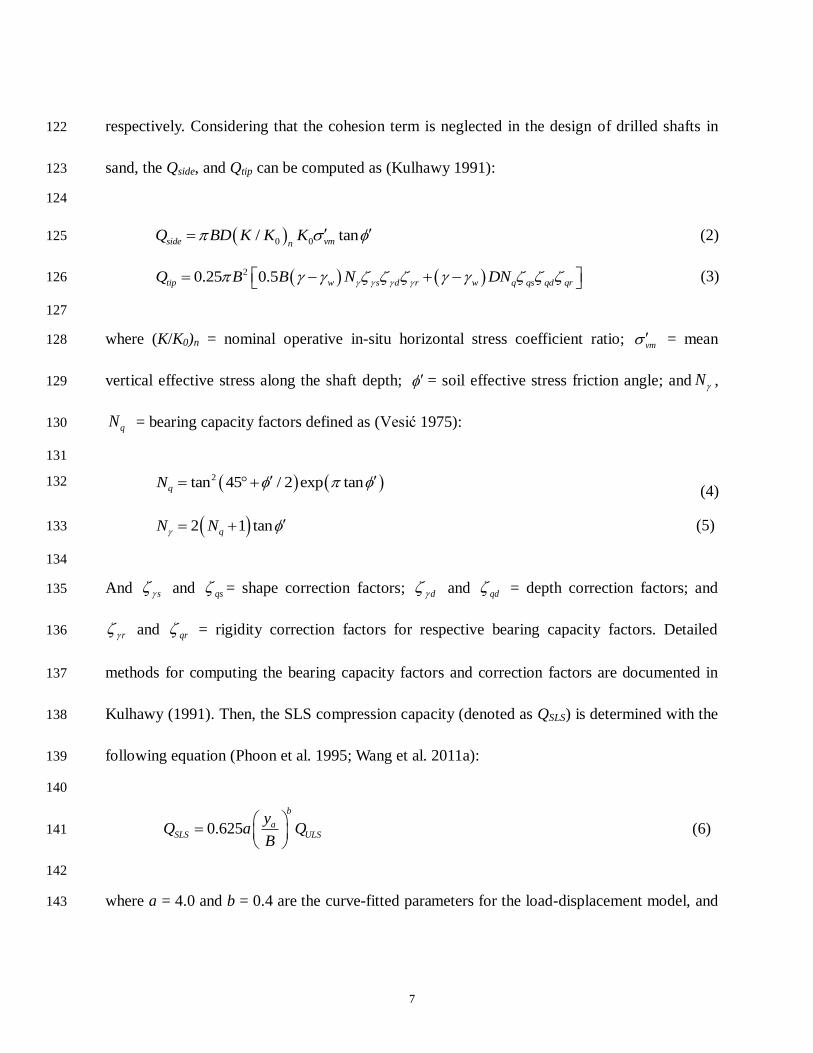
respectively. Considering that the cohesion term is neglected in the design of drilled shafts in 122
sand, the Qside, and Qtip can be computed as (Kulhawy 1991): 123
124
0 0/ tanside vmnQ BD K K K (2) 125
20.25 0.5tip w s d r w q qs qd qrQ B B N DN (3) 126
127
where (K/K0)n = nominal operative in-situ horizontal stress coefficient ratio; vm = mean 128
vertical effective stress along the shaft depth; = soil effective stress friction angle; and N , 129
qN = bearing capacity factors defined as (Vesić 1975): 130
131
2tan 45 / 2 exp tanqN (4)
132
2 1 tanqN N (5) 133
134
And s and qs = shape correction factors; d and qd = depth correction factors; and 135
r and qr = rigidity correction factors for respective bearing capacity factors. Detailed 136
methods for computing the bearing capacity factors and correction factors are documented in 137
Kulhawy (1991). Then, the SLS compression capacity (denoted as QSLS) is determined with the 138
following equation (Phoon et al. 1995; Wang et al. 2011a): 139
140
0.625
b
aSLS ULS
yQ a Q
B
(6) 141
142
where a = 4.0 and b = 0.4 are the curve-fitted parameters for the load-displacement model, and 143

8
ay = allowable displacement, which is 25mm for this problem. 144
The probability of ULS failure ( ULS
fp ) and the probability of SLS failure ( SLS
fp ) are 145
defined as 50r ULSP Q F and 50r SLSP Q F , respectively. The reliability-based design can 146
be realized by meeting the target failure probability requirements, namely, SLS SLS
f Tp p and 147
ULS ULS
f Tp p , where SLS
Tp and ULS
Tp are the target failure probabilities based on the 148
serviceability limit state and the ultimate limit state, respectively. 149
150
Methodology for Reliability-Based Robust Geotechnical Design 151
In a reliability-based RGD, the design robustness is considered explicitly in the 152
reliability-based design framework. Although the robustness may be interpreted differently (e.g., 153
Taguchi 1986; Chen et al. 1996; Doltsinis and Kang 2005; Park et al. 2006; Ait Brik et al. 2007; 154
Papadopoulos and Lagaros 2009), in this paper a geotechnical design is considered robust if the 155
performance measure (i.e., failure probability ULS
fp or SLS
fp ) is insensitive to the variation of 156
noise factors (i.e., uncertain soil parameters). Note that the probability of failure is usually 157
determined using Monte Carlo simulation (MCS) or reliability-based methods that require 158
knowledge of the variation of soil parameters. If the actual variations of soil parameters are 159
greater than the estimated variations that are used in the reliability-based analysis, the 160
probability of failure may be underestimated. Thus, the generally accepted reliability-based 161
designs that do not consider robustness in the analysis could violate the safety requirements 162
( ULS ULS
f Tp p and SLS
fp <SLS
Tp ) if the variations of soil parameters are underestimated. The 163

9
chance for this violation may be greatly reduced if the variation of the failure probability, which 164
is considered as the system response, can be minimized by adjusting design parameters. 165
Thus, in a reliability-based RGD, the goal is to achieve design robustness by adjusting 166
design parameters (such as B and D in the drilled shaft design) to minimize the variation of the 167
probability of failure. In many cases, however, greater robustness can only be achieved at a 168
high cost and thus, a trade-off exists, which can best be investigated through multi-objective 169
optimization. 170
Estimation of the coefficients of variation of soil parameters 171
As pointed out by Phoon et al. (1995), drained friction angle and coefficient of 172
earth pressure at rest K0 are the two random variables that should be considered for the 173
reliability-based design of drilled shaft in loose sand. 174
In geotechnical practice, soil parameters are often determined from a limited number of 175
test data, thus, the statistical parameters derived from a small sample may be subjected to error. 176
In general, the “population” mean can be adequately estimated from the “sample” mean even 177
with a small sample (Wu et al. 1989). However, the estimation of standard deviation of the 178
population based on a sample is often not as accurate, especially with a smaller sample. Of 179
course, the measurement error and the model with which soil parameters are derived (e.g., 180
estimation of based on SPT or other means) could also contribute to the variation of the 181
derived parameters. 182
Duncan (2000) suggested that the standard deviation of a random variable might be 183

10
obtained by (1) direct calculation from data, (2) use of published coefficient of variation (COV), 184
or (3) estimate based on the “three-sigma rule.” The evaluation of parameter uncertainty for a 185
specific problem is the duty of the engineer in charge. In this paper, the published COVs are 186
adopted for illustration of robustness concept in a geotechnical design. The COV of of 187
loose sand, denoted as [ ]COV , typically ranges from 0.05 to 0.10 (Amundaray 1994), and 188
the COV of K0, denoted as 0[ ]COV K , typically ranges from 0.20 to 0.90 (Phoon et al. 1995). 189
For a typical reliability-based design, it is reasonable to take the mean value of the range of 190
COV of a given parameter as its coefficient of variation. Thus, [ ]COV ≈ 0.07 and 191
0[ ]COV K ≈ 0.50 may be used in a reliability-based design of drilled shafts in sand if there is 192
no additional data. 193
The outcome of a reliability-based design is affected by the accuracy of the estimated 194
COVs of soil parameters. Because of the uncertainty of the estimated COVs, there will be 195
uncertainty regarding the outcome of the design (e.g., we are not sure whether the design really 196
meets the target reliability index requirement if the COVs are underestimated). In this paper, we 197
incorporate the concept of robustness to ensure that the design will meet the target reliability 198
index requirement in the face of uncertainty on the estimated COVs. 199
The uncertainty of the COV of a given soil parameter may be characterized with a range. 200
In fact, when COV is expressed as a range, the uncertainty is readily characterized. For 201
example, if we consider [ ]COV to vary from 0.05 to 0.10 based on Amundaray (1994), then 202
the uncertainty about the value of [ ]COV to be used in the reliability design is readily 203
11
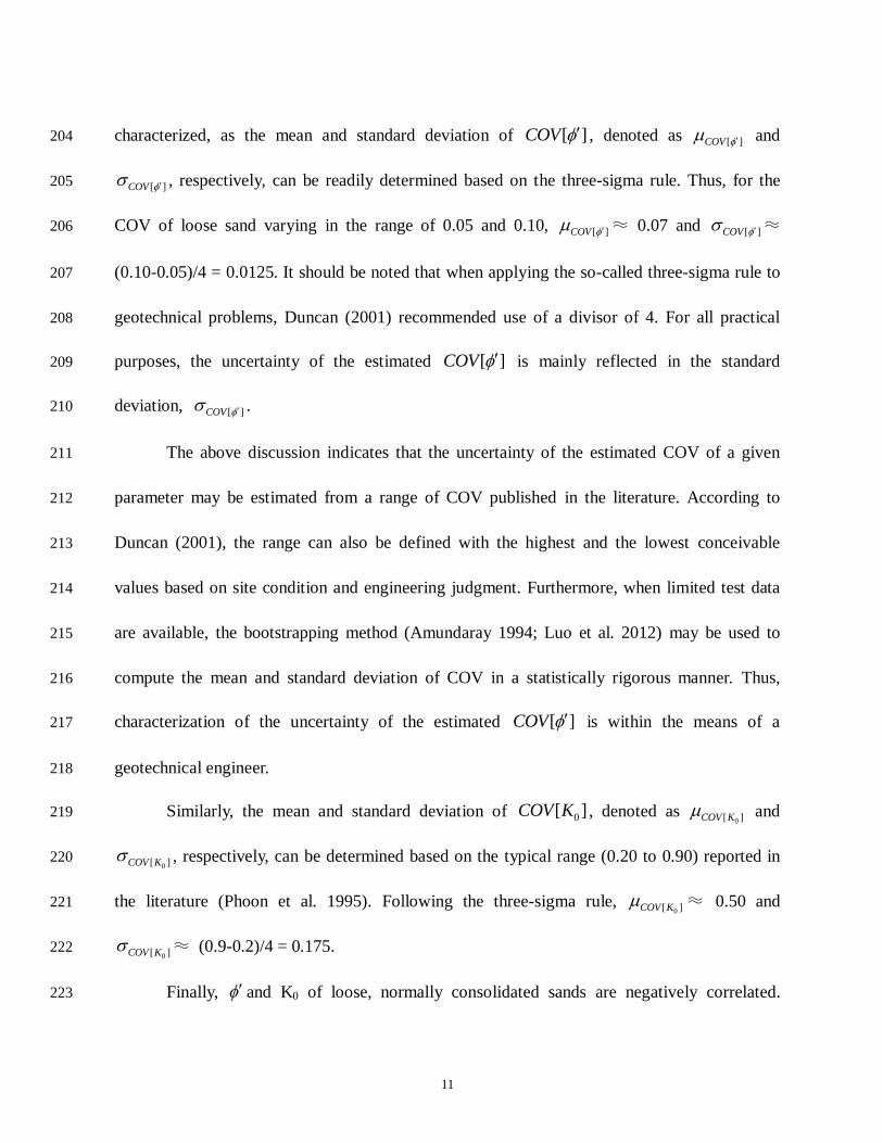
characterized, as the mean and standard deviation of [ ]COV , denoted as [ ]COV and 204
[ ]COV , respectively, can be readily determined based on the three-sigma rule. Thus, for the 205
COV of loose sand varying in the range of 0.05 and 0.10, [ ]COV ≈ 0.07 and [ ]COV ≈ 206
(0.10-0.05)/4 = 0.0125. It should be noted that when applying the so-called three-sigma rule to 207
geotechnical problems, Duncan (2001) recommended use of a divisor of 4. For all practical 208
purposes, the uncertainty of the estimated [ ]COV is mainly reflected in the standard 209
deviation, [ ]COV . 210
The above discussion indicates that the uncertainty of the estimated COV of a given 211
parameter may be estimated from a range of COV published in the literature. According to 212
Duncan (2001), the range can also be defined with the highest and the lowest conceivable 213
values based on site condition and engineering judgment. Furthermore, when limited test data 214
are available, the bootstrapping method (Amundaray 1994; Luo et al. 2012) may be used to 215
compute the mean and standard deviation of COV in a statistically rigorous manner. Thus, 216
characterization of the uncertainty of the estimated [ ]COV is within the means of a 217
geotechnical engineer. 218
Similarly, the mean and standard deviation of 0[ ]COV K , denoted as 0[ ]COV K and 219
0[ ]COV K , respectively, can be determined based on the typical range (0.20 to 0.90) reported in 220
the literature (Phoon et al. 1995). Following the three-sigma rule, 0[ ]COV K ≈ 0.50 and 221
0[ ]COV K ≈ (0.9-0.2)/4 = 0.175. 222
Finally, and K0 of loose, normally consolidated sands are negatively correlated. 223

12
According to Mayne and Kulhawy (1982), and personal communications with Mayne (2012) 224
and Phoon (2012), the correlation coefficient 0,K is estimated to be in the range of -0.6 to 225
-0.9. Following the three-sigma rule, the mean and standard deviation of 0,K , denoted as 226
, 0K
and
, 0K
, are estimated to be -0.75 and 0.075, respectively. Furthermore, for 227
illustration purpose, both and K0 are assumed to follow lognormal distribution. 228
As is shown later, the robustness of a reliability-based design is achieved if the system 229
response (in terms of the probability of failure) is insensitive to the variation of the estimated 230
COVs of and K0 and their correlation. 231
232
Reliability-based robust geotechnical design approach 233
A framework for reliability-based robust geotechnical design is presented below using 234
design of drilled shaft in loose sand as an example. This framework is a modification of the 235
authors’ recent work (Juang et al. 2012; Juang and Wang 2013; Wang et al. 2013). In reference 236
to Figure 2, the RGD approach is summarized in the following steps (presented with rationale): 237
Step 1: Select design parameters and noise factors and identify the design space. For 238
the design of drilled shaft in sand, the diameter (B) and depth (D) of the drilled shaft are 239
considered as the design parameters, and the soil parameters and K0 are considered as the 240
noise factors. The statistics of the noise factors are estimated based on available data and 241
guided by experience, as discussed previously. The choice of diameter B is usually limited to 242
equipment and local practice, and for illustration purpose in this paper, only three discrete 243
values (B = 0.9 m, 1.2 m, and 1.5 m) are considered here. The depth D is often computed for a 244

13
given B that satisfies ULS or SLS requirements, and is typically rounded to the nearest 0.2 m 245
(Wang et al. 2011a). Thus, design parameters B and D can be conveniently modeled in the 246
discrete domain and the design space will consist of finite number of designs (say, M designs). 247
For example, M will be equal to 93 if D is selected from the likely range of 2 m to 8 m (for the 248
drilled shaft shown in Figure 1 subjected to an axial compression load F50 = 800 kN) for each 249
of the three discrete B values. 250
Step 2: Evaluate the variation of the system response as a measure of robustness of a 251
given design. For each possible design in the design space, the probability of failure can be 252
computed based on either ultimate limit state (ULS) or serviceability limit state (SLS). Here, 253
the probability of failure is treated as a system response (or more precisely, an effect of the 254
system response), and the variation of the system response as a result of the variation of the 255
sample statistics of the noise factors is adopted as a measure of robustness. In this paper, the 256
modified point estimate method (PEM) by Zhao and Ono (2000) is used for evaluating the 257
mean and standard deviation of the failure probability. The PEM approach requires evaluation 258
of the failure probability at each of a set of N “estimating” points (or sampling points) of the 259
input noise factors, as reflected by the inner loop shown in Figure 2. In each repetition, 260
statistics of each of the noise factors at each PEM estimating point must be assigned, and then 261
the failure probability is computed using the First Order Reliability Method (FORM; see Ang 262
and Tang 1984; Phoon 2004). The resulting N failure probabilities are then used to compute the 263
mean and standard deviation of the failure probability. 264

14
Step 3: Repeat Step 2 for each of the M designs in the design space. For each design, 265
the mean and standard deviation of the failure probability are determined. This step is 266
represented by the outer loop shown in Figure 2. 267
Step 4: Perform a fast elitist non-dominated sorting to establish a Pareto Front. For 268
multi-objective optimization, Non-dominated Sorting Genetic Algorithm version II (NSGA-II) 269
by Deb et al. (2002) is widely used. The sorting technique of NSGA-II is adopted herein. 270
Note that in single-objective optimization, one tries to get a design that is superior to all 271
other designs. For example, in a reliability-based optimization, one may seek to find the 272
least-cost design using reliability as a constraint. Such a scheme tends to result in a design with 273
the least cost but barely meet the reliability requirement. However, this design may not be the 274
“best” solution for stakeholders who are willing to pay more for less risk. 275
When multiple objectives are enforced, it is likely that no single best design exits that is 276
superior to all other designs in all objectives. However, a set of designs may exist that are 277
superior to all other designs in all objectives; but within the set, none of them is superior or 278
inferior to each other in all objectives. These designs constitute a Pareto Front. Figure 3 shows 279
a conceptual illustration of a Pareto Front in a bi-objective setting (Gencturk and Elnashai 280
2011). Each point on the Pareto Front is optimal in the sense that no improvement can be 281
achieved in one objective without worsening in at least one other objective. When the 282
optimization process yields a Pareto Front, a trade-off situation is implied. For example, if the 283
cost and the robustness are two objectives in the trade-off relationship, the designer can 284

15
approach it in two ways. If an acceptable cost range of the design is pre-defined, the most 285
robust design within the cost range will be the best design. On the other hand, if certain level of 286
robustness is required and specified, the least cost design that meets the robustness requirement 287
will be the best design. 288
Finally, it should be noted that the procedure described above (in reference to Figure 2) 289
is only one possible implementation of the RGD methodology. Other implementations may be 290
equally effective. For example, FORM as a means to compute the failure probability for a given 291
design with a set of known statistics of each of the noise factors may be replaced by MCS. 292
Similarly, PEM as a means to compute the variation of the system response (i.e., the failure 293
probability) may also be replaced by MCS or other means. Since only finite, and relatively 294
small, number of designs are considered in this illustrative example (M = 93), only the sorting 295
part of the NSGA-II algorithm is employed for selecting “points” (or designs) for the Pareto 296
Front. However, if M becomes much larger, the full algorithm of NSGA-II may be employed 297
for the multi-objective optimization. 298
299
Reliability-Based Design without Robustness Consideration 300
To provide a reference for reliability-based RGD, reliability-based design of a drilled 301
shaft without considering robustness is first presented. For a drilled shaft shown in Figure 1 302
with soil parameters described in Table 1 (in particular, [ ]COV = 0.07, 0[ ]COV K = 0.50, 303
and 0,K = -0.75), the probability of SLS and ULS failure for various designs for a given axial 304

16
load of F50 = 800 kN is analyzed using FORM. The results are shown in Figure 4. The results 305
indicate that the SLS requirement controls the design of drilled shaft under axial compression 306
load, which is consistent with those reported by other investigators (e.g., Wang et al. 2011a). In 307
fact, in all analyses performed in this study, the SLS requirement always controls the design of 308
drilled shafts in sand for axial compression. Thus, in the subsequent analysis only the SLS 309
failure probability is considered. 310
In a reliability-based design, the reliability requirement is generally used as a constraint 311
(i.e., the actual reliability index must be greater than the target value or the corresponding 312
failure probability must be less than the target value) to screen for the acceptable designs, and 313
then the optimal design is obtained by minimizing the cost (Zhang et al. 2011). For a 314
comprehensive design, the total life-cycle cost of the structure may be considered (Frangopol 315
and Maute 2003). For simplicity, only the initial cost of a drilled shaft is considered in this 316
paper so that we can focus on the subject of design robustness. The initial cost generally refers 317
to the cost for completing a drilled shaft construction, including both material and labor cost, 318
which can be estimated from published, annually updated literature, such as Means Building 319
Construction Cost Data (R.S. Means Co. 2007). The U.S. national average unit costs for 320
constructing drilled shafts with respective diameters of 0.9 m, 1.2 m and 1.5 m are summarized 321
in Table 2. The costs for constructing a unit depth (0.3 m) are USD 77.5, 116 and 157, 322
respectively for the three diameters (Wang et al. 2011a). If the “best” design is to be chosen 323
based on least cost subjected to the constraint that the SLS failure probability is less than a 324
17
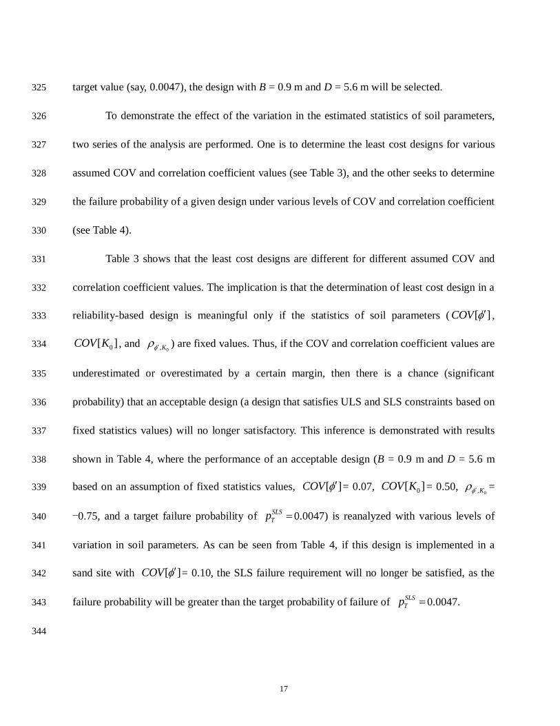
target value (say, 0.0047), the design with B = 0.9 m and D = 5.6 m will be selected. 325
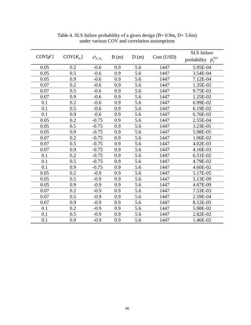
To demonstrate the effect of the variation in the estimated statistics of soil parameters, 326
two series of the analysis are performed. One is to determine the least cost designs for various 327
assumed COV and correlation coefficient values (see Table 3), and the other seeks to determine 328
the failure probability of a given design under various levels of COV and correlation coefficient 329
(see Table 4). 330
Table 3 shows that the least cost designs are different for different assumed COV and 331
correlation coefficient values. The implication is that the determination of least cost design in a 332
reliability-based design is meaningful only if the statistics of soil parameters ( [ ]COV , 333
0[ ]COV K , and 0,K ) are fixed values. Thus, if the COV and correlation coefficient values are 334
underestimated or overestimated by a certain margin, then there is a chance (significant 335
probability) that an acceptable design (a design that satisfies ULS and SLS constraints based on 336
fixed statistics values) will no longer satisfactory. This inference is demonstrated with results 337
shown in Table 4, where the performance of an acceptable design (B = 0.9 m and D = 5.6 m 338
based on an assumption of fixed statistics values, [ ]COV = 0.07, 0[ ]COV K = 0.50, 0,K = 339
-0.75, and a target failure probability of SLS
Tp 0.0047) is reanalyzed with various levels of 340
variation in soil parameters. As can be seen from Table 4, if this design is implemented in a 341
sand site with [ ]COV = 0.10, the SLS failure requirement will no longer be satisfied, as the 342
failure probability will be greater than the target probability of failure of SLS
Tp 0.0047. 343
344

18
Reliability-Based Design Considering Robustness 345
To investigate the issue of design robustness, the same drilled shaft problem (see Figure 346
1 and Table 1) is analyzed with additional knowledge of the variation of [ ]COV , 0[ ]COV K 347
and 0,K . Specially, the reliability-based design is based on the following additional data: 348
[ ]COV = 0.07, [ ]COV = 0.125, 0[ ]COV K = 0.50,
0[ ]COV K = 0.175, , 0K
= -0.75, and , 0K
349
= 0.075. It should be noted that these values are just used as an example to illustrate the concept 350
of robustness in the design, although they are deemed appropriate based on an assessment of 351
these parameters presented previously. 352
Following the procedure described previously (in reference to Figure 2), the mean and 353
standard deviation of the probability of SLS failure SLS
fp , namely p and p , can be 354
obtained for various designs (i.e., various pairs of B and D). Figure 5 shows the mean SLS 355
failure probability ( p ) for various designs. As can be seen, many designs have a mean failure 356
probability greater than the target failure probability (SLS
Tp 0.0047). Figure 6 shows the 357
standard deviation of the SLS failure probability ( p ). Note that in this figure, only acceptable 358
designs (those that have a p less than the target failure probability) are plotted. 359
It is noted that the robustness of a reliability-based design, in which acceptance of the 360
design is based on the requirement that SLS SLS
f Tp p , may be measured in terms of the standard 361
deviation of the SLS failure probability ( p ). Thus, a design is said to have a greater 362
robustness if p caused by the uncertainty of [ ]COV , 0[ ]COV K and 0,K is smaller. In 363
Figure 6, all designs are acceptable based on the traditional reliability-based design concept. If 364

19
the cost is the only design objective after satisfying the SLS failure requirement, then the 365
design of B = 0.9 m and D = 6.0 m will be selected, which has the least cost of 1550USD. 366
However, this design has the greatest standard deviation of the SLS failure probability, 367
indicating that the design has the lowest level of robustness or is most sensitive to the 368
uncertainty in the estimated statistics of soil parameters. The implication is that such design, 369
albeit most economical from the traditional reliability-based design viewpoint, is likely to fail 370
the SLS failure requirement if the uncertainty of soil parameters statistics is ignored. On the 371
other hand, if a design with a smaller p is chosen, it will be more robust, albeit at a higher 372
cost. 373
To further illustrate the trade-off between cost and robustness, all acceptable designs 374
(SLS
p Tp 0.0047) are computed for their costs, and these costs are plotted against robustness 375
(in terms of standard deviation of the SLS failure probability, p ). The results are shown in 376
Figure 7. Three designs, as indicated in Figure 7, are used as an example for further discussion 377
of the trade-off between cost and robustness. Design 1 (B = 0.9 m, D = 6.0 m) has the least cost 378
among all acceptable designs, while Design 2 (B = 0.9 m, D = 6.4 m) and Design 3 (B = 0.9 m, 379
D = 7.0 m) cost more but have a smaller p value (meaning that the designs are more robust). 380
For each of these three designs, the probability of SLS failure is reanalyzed for various COV 381
and correlation levels for the two soil parameters, and K0. The results of these additional 382
analyses are shown in Table 5. It is noted that the uncertainty levels of 27 cases for loose sand 383
shown in Table 5 can be roughly divided into three categories, Low variation ( [ ]COV = 0.05 384

20
and 0[ ]COV K = 0.2), Medium variation ( [ ]COV = 0.07 and 0[ ]COV K = 0.5), and High 385
variation ( [ ]COV = 0.10 and 0[ ]COV K = 0.9). 386
Based on the results shown in Table 5, Design 1 will perform satisfactory (in terms of 387
meeting the requirement that SLS SLS
f Tp p 0.0047) if the variation of soil parameters for this 388
sand is Low or Medium. However, Design 1 does not meet the SLS failure probability 389
requirement if it is implemented in a site with high variation in and K0. Thus, for this design, 390
the SLS failure probability is sensitive to the level of uncertainty of soil parameters. 391
On the contrary, with Design 3, the SLS failure probabilities under all uncertainty 392
scenarios meet the requirement. Thus, for this design, the SLS failure probability is insensitive 393
to the uncertainty in the COV levels of soil parameters. However, the cost is 1808USD for 394
Design 3, compared to the cost of 1550USD for Design 1. Finally, Design 2 is a compromise 395
between Design 1 and Design 3, in which the increase in cost is not as prohibitive (only 396
1653USD) but it still has some chance of violating the SLS failure probability requirement. 397
The results presented above suggest that design aids are needed for making more 398
informed engineering decisions. In the sections that follow, the concept of Pareto Front is 399
presented to explain the trade-off relationship between cost and robustness, followed by a 400
procedure for selecting better designs. 401
402
Two-Objective Non-dominated Sorting for Pareto Front 403
Pareto-Front consists of designs that are not dominated by other designs with respect to 404
21
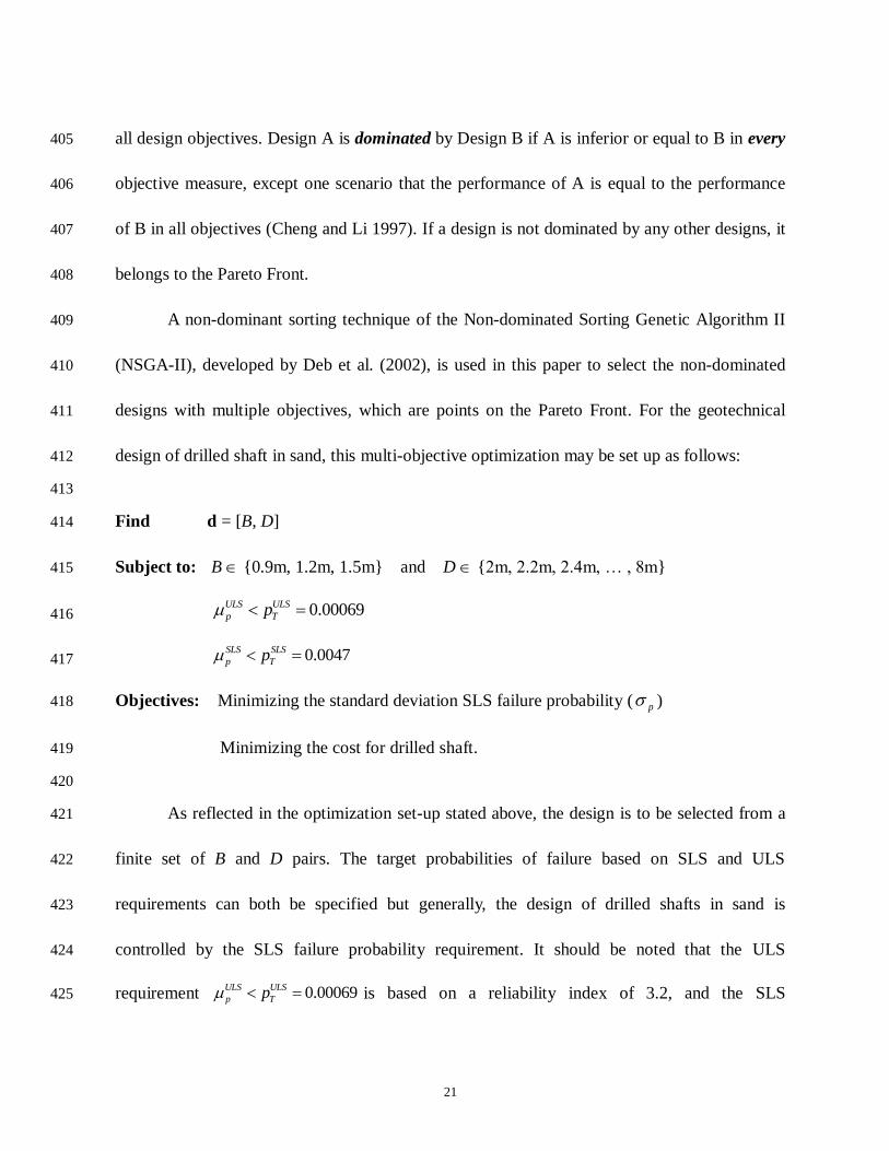
all design objectives. Design A is dominated by Design B if A is inferior or equal to B in every 405
objective measure, except one scenario that the performance of A is equal to the performance 406
of B in all objectives (Cheng and Li 1997). If a design is not dominated by any other designs, it 407
belongs to the Pareto Front. 408
A non-dominant sorting technique of the Non-dominated Sorting Genetic Algorithm II 409
(NSGA-II), developed by Deb et al. (2002), is used in this paper to select the non-dominated 410
designs with multiple objectives, which are points on the Pareto Front. For the geotechnical 411
design of drilled shaft in sand, this multi-objective optimization may be set up as follows: 412
413
Find d = [B, D] 414
Subject to: B {0.9m, 1.2m, 1.5m} and D {2m, 2.2m, 2.4m, … , 8m} 415
0.00069ULS ULS
p Tp 416
0.0047SLS SLS
p Tp 417
Objectives: Minimizing the standard deviation SLS failure probability ( p ) 418
Minimizing the cost for drilled shaft. 419
420
As reflected in the optimization set-up stated above, the design is to be selected from a 421
finite set of B and D pairs. The target probabilities of failure based on SLS and ULS 422
requirements can both be specified but generally, the design of drilled shafts in sand is 423
controlled by the SLS failure probability requirement. It should be noted that the ULS 424
requirement 0.00069ULS ULS
p Tp is based on a reliability index of 3.2, and the SLS 425

22
requirement 0.0047SLS SLS
p Tp is based on a reliability index of 2.6 (Wang et al. 2011a). 426
Although the multi-objective optimization as prescribed above can easily be carried out 427
using NSGA-II, the number of possible designs in the design space in this drilled shaft example 428
is finite and relatively small (M = 93). Thus, only the non-dominated sorting technique of 429
NSGA-II is applied herein. Among the 93 designs, 56 are found acceptable based on the SLS 430
and ULS failure probability requirements. With the non-dominated sorting, 27 of the 56 431
acceptable designs are selected into the Pareto Front (with two objectives, cost and robustness 432
in terms of p ), as shown in Figure 8. It should be noted that the non-dominated sorting is 433
generally more efficient if a larger number of acceptable designs is to be sorted for Pareto Front, 434
especially when more design parameters are involved and/or the interactions between the 435
design parameters and noise factors are much more complex. 436
While the traditional reliability-based design approach often selects the best design 437
based solely on cost, after satisfying the failure probability requirements, the reliability-based 438
robust design considers robustness in addition to cost. In the case of drilled shaft design, 439
optimization of both cost and robustness yields a Pareto Front, which enables the engineer to 440
make informed decision based on a well-defined trade-off relationship between cost and 441
robustness against the possible soil parameters variability. If a certain maximum cost is desired 442
(i.e., the cost must be less than some desired amount), then the design with greatest robustness 443
will be the best choice. If a certain minimum level of robustness is desired, then the design with 444
least cost will be the best choice. 445

23
446
Selection of the best design based on feasibility robustness 447
Although the Pareto Front provides a well-defined trade-off relationship between cost 448
and robustness, it is desirable to take the process further to ease decision making. Here, the 449
concept of “feasibility robustness” (Parkinson et al. 1993) is further adopted. The design with 450
feasibility robustness is the design that can remain “feasible” (i.e., acceptable in terms of 451
satisfying the safety and serviceability requirements) in a pre-defined constraint for certain 452
probability even when it undergoes variations. In this paper, the feasibility robustness is the 453
robustness against the SLS failure requirement,
SLS SLS
f Tp p 0.0047. Because of the 454
uncertainty in the estimated sample statistics, [ ]COV , 0[ ]COV K and 0,K , the SLS 455
failure probability SLS
fp may be treated as a random variable. Parkinson et al. (1993) suggest 456
that feasibility robustness can be expressed with the following constraint: 457
458
0Pr[( 0.0047) 0]SLS
fp P (7) 459
460
where Pr[( 0.0047) 0]SLS
fp is the probability that the SLS failure requirement can be 461
satisfied (and thus, the system is still feasible), and 0P is an acceptable level of this probability 462
selected by the designer. The probability Pr[( 0.0047) 0]SLS
fp is referred to herein as the 463
feasibility probability. 464
Determination of the probability Pr[( 0.0047) 0]SLS
fp requires the knowledge of 465
distribution type of SLS
fp , which is generally difficult to ascertain. Simulations of a given 466
design (for example, B = 0.9 m, D = 6.8 m) show that the resulting histogram of SLS can be 467

24
approximated well with a lognormal distribution, as depicted in Figure 9. Thus, an equivalent 468
counterpart in terms of Pr[( ) 0]SLS SLS
T , where 2.6SLS
T (corresponding to 469
SLS
Tp 0.0047), may be used to assess the feasibility robustness. 470
The mean and standard deviation of SLS , denoted as and , respectively, can 471
be determined using FORM within the framework of PEM. When SLS is assumed to follow 472
lognormal distribution, the feasibility probability can be computed using simplified procedure 473
such as first order second moment (FOSM) method as follows (Juang and Wang 2013): 474
475
Pr[( 2.6) 0] ( )ULS
(8) 476
where is the cumulative standard normal distribution function, and is defined as: 477
478
2
2
ln 1 ln 2.6
ln 1
(9) 479
480
If the acceptable level of the feasibility probability is specified as 0P = 97.72%, then 481
the required value will be 2. In other words, if the computed based on and 482
is equal to 2, then there is a feasibility probability of 97.72% that the SLS failure requirement 483
( SLS SLS
f Tp p 0.0047 or equivalently 2.6)SLS SLS
T is satisfied. 484
Thus, the value may be used as an index for feasibility robustness. Figure 10 485
shows the values computed for all 27 points on the Pareto Front versus the corresponding 486
costs. As expected, the results show that a design with higher feasibility robustness costs more. 487

25
By selecting a desired feasibility robustness level (in terms of ), the least-cost design among 488
those on the Pareto Front can readily be determined. Table 6 shows final designs selected from 489
the Pareto Front for various specified feasibility robustness levels. As a reference, it is observed 490
that the final design obtained for the feasibility robustness level of = 2, namely B = 0.9 m 491
and D = 6.8 m, is approximately the same as the threshold acceptable design that was obtained 492
by the traditional reliability-based design under the higher-end level of soil variability that was 493
examined in Table 3. The developed Pareto Front, especially with the computed feasibility 494
robustness, makes it easier to select the best design to meet the designer’s objectives. 495
496
Integration of RGD with Load and Resistance Factor Design (LRFD) 497
In the above sections, we have shown how the robust design concept can be integrated 498
with rigorous reliability methods such as FORM. To this end, the reliability-based RGD method 499
is proposed. In the current geotechnical practice, however, reliability-based design is often 500
carried out using the LRFD approach. From the user’s perspective, the LRFD approach is a 501
deterministic approach, although the parameter and model uncertainties may have been 502
considered in the calibration of resistance factors using a database of load test results. The 503
LRFD approach is often regarded as an approximate way to achieve the objective of a 504
reliability-based design, which is to maintain an acceptable and consistent safety level 505
throughout the design of all components. Because it is a deterministic approach and does not 506
require statistical characterization of soil parameters on the part of the user, the LRFD approach 507
is easier to use and more practical. However, the desire for simplicity and practicality naturally 508
comes at the expense of the flexibility and versatility that are possible with the reliability-based 509
design. For example, as noted by Wang et al. (2011b), LRFD codes are only calibrated for some 510
26
predefined value of target failure probability, which limits designer’s flexibility in selecting a 511
proper target failure probability for a particular project. Furthermore, the adopted LRFD code 512
may not address the effect of site-specific soil variability and the dependency of the bias factor 513
on the design parameters (Kulhawy et al. 2012). Previous studies by Phoon et al. (2003) and 514
Paikowsky et al. (2004) also recognized the shortcoming of the LRFD code in dealing with 515
these issues. 516
Development of “robust” resistance factors for LRFD so that the result (i.e., final design) 517
is insensitive to (or robust against) the “noises” such as site-specific soil variability and the 518
dependency of the bias factor on the design parameters is one possible solution to dilemma 519
discussed previously. In this paper, however, a simpler approach is taken, which utilizes the 520
current LRFD approach with fixed resistance factors. In the remaining of this section, we 521
demonstrate how robust design can be integrated into the current LRFD approach. 522
The general form of a LRFD method (Phoon et al. 1995; Phoon et al. 2003; Paikowsky 523
et al. 2004; AASHTO 2007; FHWA 2010; Roberts et al. 2011; Kulhawy et al. 2012; Basu and 524
Salgado 2012) may be expressed as follows: 525
Ψn nF Q (10) 526
where is load factor ( 1) ; Ψ is resistance factor ( 1) ; Fn is the nominal load; Qn is the 527
nominal resistance. The load factor from structural engineering is generally adopted in 528
foundation design to maintain design consistency (Ellingwood et al. 1982a,b). 529
The LRFD method has been successfully used in structural engineering, where the 530
variation of input parameters and nominal resistance is typically low. However, the variation 531
for soil parameters can be much higher, which demands a smaller resistance factor to 532
compensate for the effect of larger variation in the nominal resistance. As a user of a particular 533

27
LRFD code or method, however, the resistance factor is fixed. Thus, in a site where the 534
variation of soil parameters is high, it would be a challenging task to select nominal parameter 535
values for design regardless of whether the LRFD or the traditional factor-of-safety-based 536
approach is taken. 537
The focus of this section is to investigate how the proposed RGD methodology can be 538
integrated with LRFD method. In particular, we seek an answer to the question, “how can the 539
design of drilled shafts by means of the LRFD method be “robust” in the face of uncertainty?” 540
In other words, as a user, how do we ensure that the design requirement as specified in Eq. (10) 541
is satisfied with the estimated nominal parameter values? 542
To answer the above question, let us consider the design example of drilled shaft in sand 543
subjected to drain compression loading (see Figure 1). The LRFD formulation developed with 544
generalized reliability theory (Phoon et al. 1995) is adopted as the deterministic model. 545
Specifically, the ULS and SLS design equations for drilled shaft under drained compression is 546
written as: 547
50 Ψ Ψ Ψs sN t tN wF Q Q W (11) 548
50 Ψc cNF Q (12) 549
550
where F50 is the factored load based on 50-year return period, which is the left-hand-side of Eq. 551
(10); Ψs is the resistance factor for side resistance; QsN is the nominal side resistance; Ψt is 552
the tip resistance factor; QtN is the nominal tip resistance; Ψw is the weight resistance factor; 553
W is the foundation weight; Ψc is the deformation factor; QcN is the nominal allowable 554
compression capacity. The resistance factors are given by Phoon et al. (1995) as follows: 555
Ψs 0.42, Ψ =t 0.39, Ψ =w 0, and Ψ =c 0.56. The nominal resistances QsN, QtN, and QcN are 556

28
calculated based on nominal values of soil parameters, including and K0. The reader is 557
referred to Phoon et al. (1995) for detailed equations for QsN, QtN, and QcN. 558
As discussed previously, the determination of nominal values for and K0 involves 559
certain degree of uncertainty. For illustration purpose, let us assume site investigation and 560
testing program yields statistics of these soil parameters as those shown in Table 1. These 561
sample statistics are considered fixed values. With the recognition of the variation of these soil 562
parameters as shown in Table 1, the LRFD requirements may be re-written as limit states: 563
564
50() Ψ Ψ ΨULS s sN t tN wg Q Q W F (13) 565
50() ΨSLS c cNg Q F (14) 566
567
In a deterministic approach, a design is said to satisfy the LRFD requirements if 568
0ULSg and 0SLSg . Because of the uncertainty of the soil parameters involved, however, 569
the predicted values of , , and sN tN cNQ Q Q , and thus ULSg and SLSg , are no longer fixed 570
numbers. Instead of checking whether the LRFD requirements of 0ULSg and 0SLSg are 571
satisfied in a yes-or-no manner, new criterion is needed. To this end, the concept of “feasibility 572
robustness” described previously is again employed. Here, robust design is aimed at finding a 573
design (i.e., a pair of design parameters B and D) so that a certain confidence level (i.e., a 574
probability) can be achieved that the LRFD requirement will be satisfied in the face of 575
uncertainty. In other words, the design can remain “feasible” in terms of satisfying the LRFD 576
requirement at a prescribed probability level. 577
For the drilled shaft example analyzed, the probability of satisfying or exceeding 578
ULS-based LRFD requirement, denoted as Pr[ () 0]ULSg , is always greater than the probability 579

29
of satisfying or exceeding SLS-based LRFD requirement, denoted as Pr[ () 0]SLSg , for all 580
designs in the design space (illustrated later in Figure 11). Thus, the SLS-based LRFD 581
requirement controls the design in this example, and only this requirement is focused in the 582
subsequent discussion. The feasibility robustness requirement is defined as: 583
584
50 0Pr[ () 0] Pr[(Ψ ) 0]SLS c cNg Q F P (15) 585
586
where 50Pr[(Ψ ) 0]c cNQ F is the probability of satisfying or exceeding the SLS-based LRFD 587
requirement, which is a measure of feasibility robustness; and 0P is a target feasibility 588
probability. A requirement of 0P = 0.5 is approximately equivalent to the deterministic 589
SLS-based LRFD requirement assessed with the mean nominal parameter values. A 590
requirement of 0P > 0.5 is desirable and needed to assure a higher chance of satisfying or 591
exceeding the LRFD requirement in the face of parameter uncertainty. 592
For convenience of presentation, the probability of satisfying or exceeding the LRFD 593
requirement, 50Pr[(Ψ ) 0]c cNQ F , is referred to hereinafter as the probability of exceedance 594
( EP ). Figure 11 shows the probability of satisfying or exceeding the ULS- and SLS-based 595
LRFD requirements, denoted as ULS
EP and SLS
EP , respectively. Designs with EP > 0.5 are 596
desired as noted previously. 597
Assuring a higher probability of exceedance in the face of uncertainty will likely cost 598
more. Thus, in the face of uncertainty, the essence of robust design is to find a design (i.e., a 599
pair of design parameters B and D) that satisfies the deterministic LRFD requirement, 600
maximizes the probability of exceedance, and minimizes the cost. As was discussed previously, 601
a single best design that satisfies all requirements usually does not exist. Rather, a Pareto Front 602
30
may exist that offers a set of non-dominated designs. Thus, a multi-objective optimization can 603
be set up to find the Pareto Front: 604
605
Find d = [B, D] 606
Subject to: B {0.9m, 1.2m, 1.5m} and D {2m, 2.2m, 2.4m, … , 8m} 607
0 and 0ULS SLS
g g 608
Objectives: Maximizing the probability of exceedance 609
Minimizing the cost for drilled shaft. 610
611
It is noted that the deterministic LRFD requirement is satisfied by the constraints of 612
0ULS
g and 0SLS
g , where ULS
g and SLS
g are the mean values of ULSg
and SLSg , 613
respectively. These mean values may be determined with sample statistics shown in Table 1 614
using PEM method (Zhao and Ono 2000). Alternatively, they may be approximately 615
determined using the deterministic approach with mean input parameter values. It should be 616
noted that the constraints of 0ULS
g and 0SLS
g are equivalent to the constraints based on 617
the probability of exceedance 0.5ULS
EP and 0.5SLS
EP . 618
The probability of exceedance EP (or more specifically, SLS
EP , since it controls the 619
design of drilled shaft in sand) may be obtained through a reliability analysis using FORM. 620
Greater probability of exceedance signals a more robust design in the face of uncertainty. 621
Alternatively, the mean and standard deviation of SLSg , denoted as SLS
g and SLS
g , 622
respectively, may be determined using PEM (Zhao and Ono 2000), from which the probability 623
of exceedance can be determined. Furthermore, from the perspective of robust design, we want 624

31
to maximize SLS
g (for safety) and minimize SLS
g (for robustness). Thus, the ratio of 625
SLS
g over SLS
g can also serve as a robustness measure. In fact, it is analog to the 626
signal-to-noise ratio (SNR) commonly used in the fields of Industrial Engineering and 627
Electrical Engineering (Taguchi 1986). For convenience, this robustness measure is referred to 628
herein as Robustness Index ( IR ). It should be noted that this Robustness Index ( IR ) is analog 629
to the reliability index using FORM that adopts Eq. (14) as limit state. 630
Figure 12 shows the Pareto Front obtained from non-dominant sorting procedure of 631
NSGA-II, which shows a more robust design (greater Robustness Index) generally costs more 632
in this case. Here, selected levels of probability of exceedance are also plotted as a reference to 633
the Robustness Index. Note that each point on the Pareto Front represents a non-dominated 634
design, a unique set of B and D in this drilled shaft example. The least cost design on this 635
Pareto Front is B = 0.9 m and D = 6.4 m, which has a cost of 1653USD and a Robustness Index 636
of IR = 0.05 (corresponding to a probability of exceedance of EP = 0.522 or 52.2%). If the 637
probability of exceedance of EP = 0.7 (or 70%) is desired, the least cost design on the Pareto 638
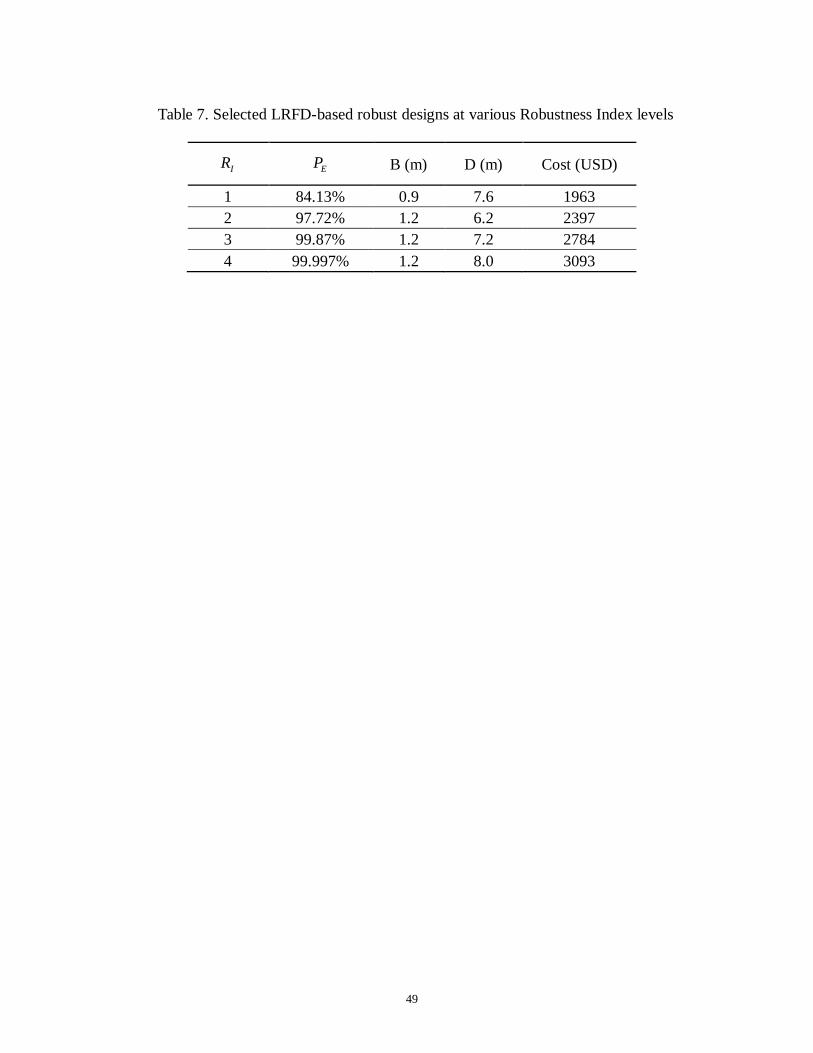
Front would be B = 0.9 m and D = 7.0 m with a cost of 1808USD. Table 7 shows examples of 639
final designs (least cost designs) selected from the Pareto Front for various target Robustness 640
Index values. Thus, the developed Pareto Front makes it easier to select the best design to meet 641
the designer’s objectives. 642
643
Further Discussions 644
The results presented previously clearly illustrated the need for, and the significance and 645
solution of, robust design to handle the uncertainty in the noise factors. Although the robust 646
32
geotechnical design (RGD) methodology presented is far from perfect, and indeed several 647
outstanding issues are still being examined in an ongoing study, this paper is considered a first 648
step, and an important step, in developing the RGD methodology. A brief description of the 649
issues that are being investigated is provided below. 650
First, the advantages of Pareto Front for identifying the best designs of drilled shaft as 651
presented in this paper are not fully realized, as the number of possible designs in the design 652
space is finite and relatively small in the example presented. In this case, the robustness and 653
cost of each possible design can be calculated, as there are only a limited number of 654
combinations of B and D. The advantages of using Pareto Front will become more obvious 655
when more design parameters are involved, more selections of discrete design parameters are 656
implemented (so that the discrete variables are getting closer to being continuous random 657
variables), and/or the interactions between the design parameters and noise factors are more 658
complex. For example, in an ongoing study of robust design of a braced excavation system, the 659
advantages of Pareto Front for identifying the best designs through multi-objectives 660
optimization become more obvious. 661
Second, robust design concept can be implemented to a deterministic (i.e., factor of 662
safety-based or LRFD) approach or a probabilistic (i.e., reliability-based) approach. Robustness 663
concept may be implemented in different ways to adapt to the domain problem and/or the 664
solution approach (deterministic or probabilistic approach). In either approach, the presented 665
RGD methodology can be adjusted slightly to adapt to the domain problem. 666
Third, although the robustness concept has been demonstrated in this paper, further 667
studies to consider robustness against other sources of uncertainty are warranted. In particular, 668
design robustness against the following uncertainties may also be considered: (1) the 669

33
distribution type of the input random variables (noise factors), (2) the effect of spatial 670
correlation distance, (3) the loading complexity, and (4) the effect of construction noise. 671
672
Summary and Concluding Remarks 673
Robustness as one of the design objectives has been illustrated in this paper. In fact, the 674
concept of robustness is incorporated into the reliability-based design to deal with the 675
uncertainty in the estimated sample statistics of soil parameters, which is often a major problem 676
in a reliability-base design. In the context of robust geotechnical design of drilled shafts for 677
axial load in sand, B (diameter) and D (depth or length) are considered as the design parameters 678
(denoted as d), and the soil parameters and K0 are considered as the noise factors (denoted 679
as z). In the reliability-based design, the safety and serviceability requirements are satisfied by 680
meeting the constraint, ( ) 0.0047SLS SLS
f Tp p d,z . It is noted that probability of the SLS failure 681
( )SLS
fp d,z is a random variable, the value of which depends on both design parameters d and 682
noise factors z. The essence of robustness design is to minimize the variation of ( )SLS
fp d,z 683
caused by the uncertainty in the estimated sample statistics of soil parameters by adjusting the 684
design parameters. 685
To consider the robustness of the design against the uncertainty in the estimated sample 686
statistics of soil parameters, the standard deviation of the SLS failure probability ( )SLS
fp d,z is 687
adopted as a measure of robustness. It is considered along with cost as the design objectives, 688
and as a result, a Pareto Front is established through non-dominated sorting. This Pareto Front 689
34
gives a trade-off relationship between cost and robustness. To improve the decision making 690
process further, the concept of feasibility robustness is adopted. Through an implementation of 691
feasibility robustness, the best design can be selected from the Pareto Front based on the 692
designer’s objectives. 693
The Robust Geotechnical Design (RGD) methodology is demonstrated through an 694
application to design of drilled shafts in sand. Although the advantages of this RGD 695
methodology have not been fully realized because the problem is fairly simple (since the design 696
space consists of finite pairs of two design parameters B and D), the methodology has been 697
shown effective in addressing the issue of design robustness. Furthermore, the RGD 698
methodology yields a Pareto Front that describes a trade-off relationship between cost and 699
robustness. Finally, the index for feasibility robustness is shown to be an effective design aid 700
that can be used to select the best design from a Pareto Front. 701
The RGD methodology can also be applied to a deterministic design approach such as 702
LRFD method. Robustness Index defined in this paper is shown effective as a robustness 703
measure for implementing robust design concept in the drilled shaft design using LRFD. As in 704
the reliability-based RGD, the dilemma of the parameter uncertainty at a given site is overcome 705
with the Pareto Front developed by implementing robustness in the LRFD approach. 706
It should be noted that the RGD is not a methodology to compete with the traditional 707
design approaches; rather, it is a complementary design strategy. With the RGD approach, the 708
focus is to satisfy three design objectives, namely safety (including strength and serviceability 709

35
requirements), cost, and robustness. Robustness, which is often not considered explicitly in 710
geotechnical design, may have to be achieved at a higher cost, and thus, development of Pareto 711
Front as a design aid through multi-objective optimization is often required for trade-off 712
consideration in the design. This paper is a first step in developing the RGD methodology. 713
Further investigation is warranted to advance this design methodology. 714
715
ACKNOWLEDGMENTS 716
The study on which this paper is based is supported in part by National Science 717
Foundation through Grant CMMI-1200117 (“Transforming Robust Design Concept into a 718
Novel Geotechnical Design Tool”) and the Glenn Department of Civil Engineering, Clemson 719
University. The results and opinions expressed in this paper do not necessarily reflect the view 720
and policies of the National Science Foundation. 721
722
723

36
References 724
American Association of State Highway and Transportation Officials (2007). LRFD bridge 725
design specifications, 4th Ed., AASHTO, Washington, DC. 726
Ait Brik, B., Ghanmi, S., Bouhaddi N., and Cogan S. (2007). “Robust design in structural 727
mechanics.” International Journal for Computational Methods in Engineering Science and 728
Mechanics, 8(1), 39–49. 729
Amundaray, J. I. (1994). “Modeling geotechnical uncertainty by bootstrap resampling.” Ph.D. 730
thesis, Purdue University, West Lafayette, IN. 731
Ang, A. H. S., and Tang, W. H. (1984). Probability concepts in engineering planning and 732
design. Vol. II: Decision, risk, and reliability, Wiley, New York. 733
Basu, D. and Salgado, R. (2012). “Load and resistance factor design of drilled shaft in sand.” 734
Journal of Geotechnical and Geoenvironmental Engineering, 138(12), 1455–1469. 735
Chen, W., Allen, J.K., Mistree, F. and Tsui, K.-L. (1996). “A procedure for robust design: 736
minimizing variations caused by noise factors and control factors.” Journal of Mechanical 737
Design, 118(4), 478–485. 738
Cheng, F.Y., and Li, D. (1997). “Multi-objective optimization design with Pareto genetic 739
algorithm.” Journal of Structural Engineering, 123(9), 1252–1261. 740
Deb, K., Pratap, A., Agarwal, S., and Meyarivan, T. (2002). “A fast and elitist multiobjective 741
genetic algorithm: NSGA-II.” IEEE Transactions on Evolutionary Computation, 6(2), 742
182–197. 743

37
Doltsinis, I., and Kang, Z. (2005). “Robust design of non-linear structures using optimisation 744
methods.” Computer Methods in Applied Mechanics and Engineering, 194(12–16), 745
1779–1795. 746
Duncan, J.M. (2000). “Factors of safety and reliability in geotechnical engineering.” Journal of 747
Geotechnical and Geoenvironmental Engineering, 126 (4), 307–316. 748
Duncan, J.M. (2001). “Closure to factors of safety and reliability in geotechnical engineering.” 749
Journal of Geotechnical and Geoenvironmental Engineering, 126 (8), 717–721. 750
Ellingwood, B., Galambos, T., MacGregor, J., and Cornell, C. (1982a). “Probability Based 751
Load Criteria—Assessment of Current Design Practices.” Journal of the Structural 752
Division, 108(5), 959–977. 753
Ellingwood, B., Galambos, T., MacGregor, J., and Cornell, C. (1982b). “Probability Based 754
Load Criteria—Load Factors and Load Combinations.” Journal of the Structural Division, 755
108(5), 978–997. 756
Federal Highway Administration (2010). “Drilled shafts: Construction procedures and LRFD 757
design methods.” Publication No. FHWA-NHI-10-016; GEC No. 10 (eds D. A. Brown, J. P. 758
Turner, and R. J. Castelli), Federal Highway Administration, Washington, DC. 759
Frangopol, D.M., and Maute, K. (2003). “Life-cycle reliability-based optimization of civil and 760
aerospace structures.” Computers and Structures, 81, 397–410. 761
Gencturk, B., and Elnashai, A. S. (2011). “Multi-objective optimal seismic design of buildings 762
using advanced engineering materials,” Mid-America Earthquake (MAE) Center, Research 763
38
Report 11-01, Department of Civil and Environmental Engineering, University of Illinois at 764
Urbana-Champaign, IL. 765
Hohenbichler, M., and Rackwitz, R. (1981). “Non-normal dependent vectors in structural 766
safety.” Journal of the Engineering Mechanics Division, 107(6), 1227–1238. 767
Juang, C. H., and Wang, L. (2013). “Reliability-based robust geotechnical design of spread 768
foundations using multi-objective genetic algorithm.” Computers and Geotechnics, 48, 769
96–106. 770
Juang, C.H., Wang, L., Atamturktur, S., and Luo, Z. (2012). “Reliability-based robust and 771
optimal design of shallow foundations in cohesionless soil in the face of uncertainty.” 772
Journal of GeoEngineering, 7(3), 75–87. 773
Kulhawy, F. H. (1991). “Drilled shaft foundations.” Foundation engineering handbook, 2nd 774
Ed., H. Y. Fang, ed.,Van Nostrand Reinhold, New York, 537–552. 775
Kulhawy, F. H., Phoon, K. K., and Wang, Y. (2012). “Reliability based design of foundations 776
–a modern view.” Proceedings of GeoCongress 2012: Geotechnical Engineering State of 777
the Art and Practice (GSP 226), Ed. K. Rollins, & D. P. Zekkos, ASCE, Reston (VA), 778
102-121. 779
Luo, Z., Atamturktur, S., and Juang, C.H. (2012). “Bootstrapping for characterizing the effect 780
of uncertainty in sample statistics for braced excavations.” Journal of Geotechnical and 781
Geoenvironmental Engineering, 139(1), 13–23. 782
39
Mayne, P.W., and Kulhawy, F.H. (1982). “Ko-OCR relationships in soil.” Journal of the 783
Geotechnical Engineering Division, 108(6), 851-872. 784
Paikowsky, S. G., Birgisson, B., McVay, M., Nguyen, T., Kuo, C., Baecher, G., Ayyub, B., 785
Stenersen, K., O’Malley, K., Chernauskas, L., and O’Neill, M. (2004). “Load and resistance 786
factor design (LRFD) for deep foundations.” NCHRP Report 507, Transportation Research 787
Board, Washington, DC. 788
Papadopoulos, V., and Lagaros, N.D. (2009). “Vulnerability-based robust design optimization 789
of imperfect shell structures.” Structural Safety, 31(6), 475–482. 790
Park, G.J., Lee, T.H., Lee, K., and Hwang, K.H. (2006). “Robust design: an overview.” AIAA 791
Journal, 44 (1), 181–191. 792
Parkinson, A., Sorensen, C., and Pourhassan, N. (1993). “A general approach for robust 793
optimal design.” Journal of Mechanical Design, 115(1), 74–80. 794
Phoon, K. K. (2004). “General non-Gaussian probability models for first order reliability 795
method (FORM): A state-of-the-art report.” ICG Rep. No. 2004-2-4 (NGI Rep. No. 796
20031091-4), International Center for Geohazards, Oslo, Norway. 797
Phoon, K. K., Kulhawy, F. H., and Grigoriu, M. D. (1995). “Reliability based design of 798
foundations for transmission line structures.” Rep. TR-105000, Electric Power Research 799
Institute, Palo Alto, California. 800

40
Phoon, K. K., Kulhawy, F. H., and Grigoriu, M. D. (2003). “Development of a reliability-based 801
design framework for transmission line structure foundations.” Journal of Geotechnical and 802
Geoenvironmental Engineering, 129(9), 798–806. 803
R. S. Means Co. (2007). R. S. Means building construction cost data, Kingston, Mass. 804
Roberts, L., Fick, D., and Misra, A. (2011). “Performance-based design of drilled shaft bridge 805
foundations.” Journal of Bridge Engineering, 16(6), 749–758. 806
Taguchi, G. (1986). Introduction to quality engineering: Designing quality into products and 807
processes, Quality Resources, White Plains, New York. 808
Tsui, K.-L. (1992). “An overview of Taguchi method and newly developed statistical methods 809
on robust design.” IIE Transactions, 24 (5), 44–57. 810
Vesić, A. S. (1975). “Bearing capacity of shallow foundations.” Foundation engineering 811
handbook, H. F. Winterkorn and H. Y. Fang, eds., Van Nostrand Reinhold, New York, 812
121–147. 813
Wang, L., Hwang, J.H., Juang, C.H., and Atamturktur, S. (2013). “Reliability-based design of 814
rock slopes – A new perspective on design robustness.” Engineering Geology, 154, 56–63. 815
Wang, Y., Au, S. K., and Kulhawy, F. H. (2011a). “Expanded reliability-based design approach 816
for drilled shafts.” Journal of Geotechnical and Geoenvironmental Engineering, 137(2), 817
140–149. 818

41
Wang, Y., Cao, Z., and Kulhawy, F.H. (2011b). “A comparative study of drilled shaft design 819
using LRFD and Expanded RBD.” Proceedings of Georisk 2011: Geotechnical Risk 820
assessment & management, GSP No. 224, Atlanta, 648-655. 821
Wu, T.H., Tang W.H., Sangrey, D.A., and Baecher, G.B. (1989). “Reliability of offshore 822
foundations—State-of-the-art.” Journal of Geotechnical Engineering, 115(2), 157–178. 823
Zhao, Y. G., and Ono, T. (2000). “New point estimates for probability moments.” Journal of 824
Engineering Mechanics, 126(4), 433–436. 825
Zhang, J., Zhang, L.M., and Tang, W.H. (2011). “Reliability-based optimization of 826
geotechnical systems.” Journal of Geotechnical and Geoenvironmental Engineering, 827
137(12), 1211–1221. 828
829

42
Lists of Tables
Table 1. Sample statistics of soil parameters
Table 2. Summary of drilled shaft unit construction cost (data from R.S. Means Co. 2007)
Table 3. Least-cost designs under various COV and correlation assumptions for soil parameters
Table 4. SLS failure probability of a given design (B = 0.9m, D = 5.6m) under various COV
and correlation assumptions
Table 5. Comparison of SLS failure probability for three designs under various COV
and correlation assumptions for soil parameters
Table 6. Selected reliability-based RGD designs at various feasibility robustness levels
Table 7. Selected LRFD-based robust designs at various Robustness Index levels
43
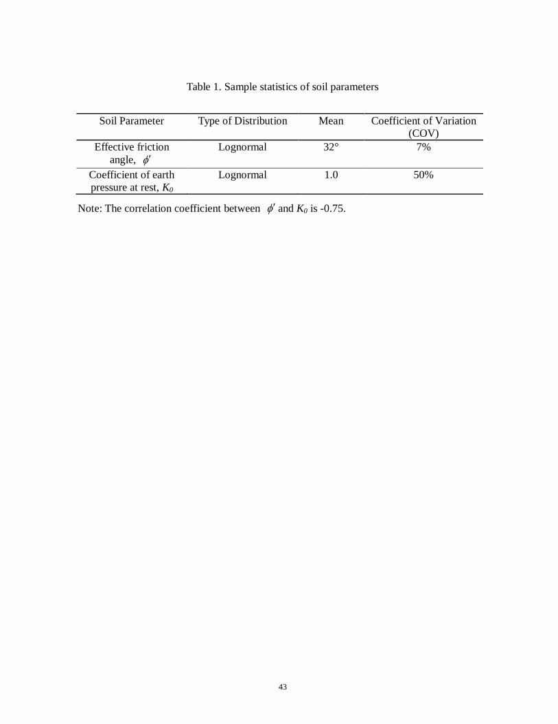
Table 1. Sample statistics of soil parameters
Soil Parameter Type of Distribution Mean Coefficient of Variation
(COV)
Effective friction
angle, Lognormal 32° 7%
Coefficient of earth
pressure at rest, K0
Lognormal 1.0 50%
Note: The correlation coefficient between and K0 is -0.75.
44
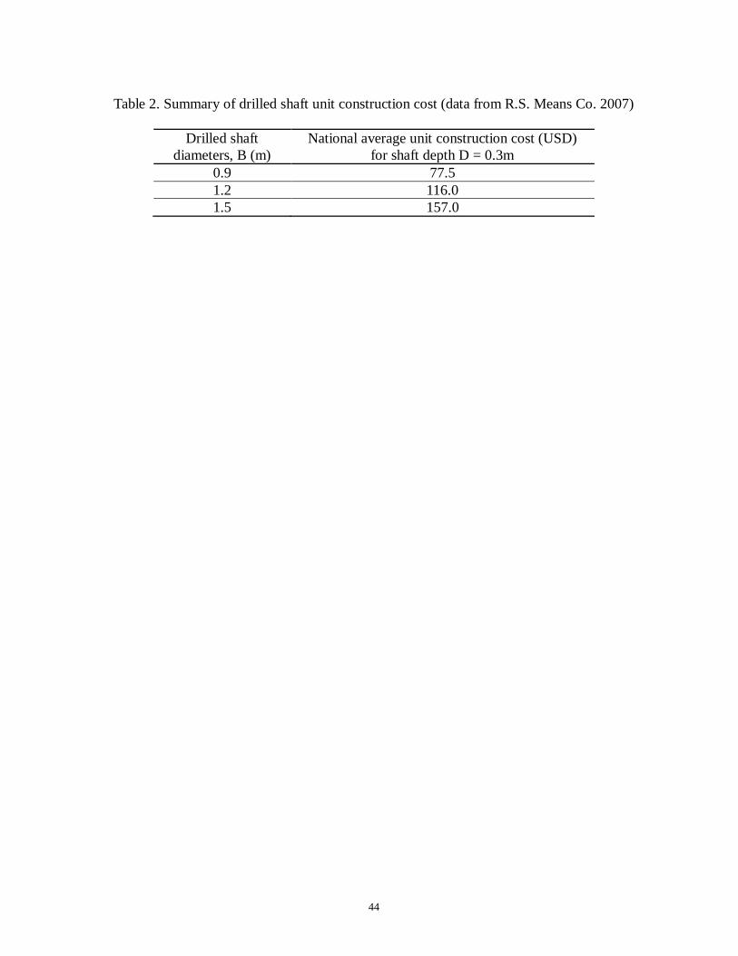
Table 2. Summary of drilled shaft unit construction cost (data from R.S. Means Co. 2007)
Drilled shaft
diameters, B (m)
National average unit construction cost (USD)
for shaft depth D = 0.3m
0.9 77.5
1.2 116.0
1.5 157.0

45
Table 3. Least-cost designs under various COV and correlation assumptions for soil parameters
[ ]COV 0[ ]COV K 0,K
B (m) D (m) Cost (USD) SLS failure
probability SLS
fp
0.05 0.2 -0.6 0.9 5.4 1395 0.00188
0.05 0.5 -0.6 0.9 5.2 1343 0.00356
0.05 0.9 -0.6 1.2 3.6 1392 0.00395
0.07 0.2 -0.6 0.9 6.0 1550 0.00362
0.07 0.5 -0.6 0.9 6.0 1550 0.00230
0.07 0.9 -0.6 0.9 6.0 1550 0.00343
0.1 0.2 -0.6 0.9 7.0 1808 0.00458
0.1 0.5 -0.6 0.9 7.0 1808 0.00297
0.1 0.9 -0.6 0.9 7.0 1808 0.00431
0.05 0.2 -0.75 0.9 5.2 1343 0.00350
0.05 0.5 -0.75 0.9 5.0 1292 0.00373
0.05 0.9 -0.75 0.9 5.0 1292 0.00428
0.07 0.2 -0.75 0.9 6.0 1550 0.00232
0.07 0.5 -0.75 0.9 5.6 1447 0.00402
0.07 0.9 -0.75 0.9 5.6 1447 0.00416
0.1 0.2 -0.75 0.9 7.0 1808 0.00304
0.1 0.5 -0.75 0.9 6.6 1705 0.00316
0.1 0.9 -0.75 0.9 6.6 1705 0.00326
0.05 0.2 -0.9 0.9 5.2 1343 0.00185
0.05 0.5 -0.9 0.9 4.8 1240 0.00207
0.05 0.9 -0.9 0.9 4.8 1240 0.00089
0.07 0.2 -0.9 0.9 5.8 1498 0.00317
0.07 0.5 -0.9 0.9 5.4 1395 0.00151
0.07 0.9 -0.9 0.9 5.2 1343 0.00256
0.1 0.2 -0.9 0.9 6.8 1757 0.00328
0.1 0.5 -0.9 0.9 6.2 1602 0.00207
0.1 0.9 -0.9 0.9 6.0 1550 0.00207
46
Table 4. SLS failure probability of a given design (B= 0.9m, D= 5.6m)
under various COV and correlation assumptions
[ ]COV 0[ ]COV K 0,K
B (m) D (m) Cost (USD) SLS failure
probability SLS
fp
0.05 0.2 -0.6 0.9 5.6 1447 5.95E-04
0.05 0.5 -0.6 0.9 5.6 1447 3.54E-04
0.05 0.9 -0.6 0.9 5.6 1447 7.12E-04
0.07 0.2 -0.6 0.9 5.6 1447 1.35E-02
0.07 0.5 -0.6 0.9 5.6 1447 9.75E-03
0.07 0.9 -0.6 0.9 5.6 1447 1.25E-02
0.1 0.2 -0.6 0.9 5.6 1447 6.99E-02
0.1 0.5 -0.6 0.9 5.6 1447 6.19E-02
0.1 0.9 -0.6 0.9 5.6 1447 6.76E-02
0.05 0.2 -0.75 0.9 5.6 1447 2.55E-04
0.05 0.5 -0.75 0.9 5.6 1447 3.23E-05
0.05 0.9 -0.75 0.9 5.6 1447 5.98E-05
0.07 0.2 -0.75 0.9 5.6 1447 1.06E-02
0.07 0.5 -0.75 0.9 5.6 1447 4.02E-03
0.07 0.9 -0.75 0.9 5.6 1447 4.16E-03
0.1 0.2 -0.75 0.9 5.6 1447 6.51E-02
0.1 0.5 -0.75 0.9 5.6 1447 4.79E-02
0.1 0.9 -0.75 0.9 5.6 1447 4.60E-02
0.05 0.2 -0.9 0.9 5.6 1447 5.17E-05
0.05 0.5 -0.9 0.9 5.6 1447 5.13E-09
0.05 0.9 -0.9 0.9 5.6 1447 4.67E-09
0.07 0.2 -0.9 0.9 5.6 1447 7.53E-03
0.07 0.5 -0.9 0.9 5.6 1447 2.59E-04
0.07 0.9 -0.9 0.9 5.6 1447 8.12E-05
0.1 0.2 -0.9 0.9 5.6 1447 5.98E-02
0.1 0.5 -0.9 0.9 5.6 1447 2.82E-02
0.1 0.9 -0.9 0.9 5.6 1447 1.46E-02

47
Table 5. Comparison of SLS failure probability for three designs under various COV and
correlation assumptions for soil parameters
[ ]COV 0[ ]COV K 0,K
SLS failure probability, SLS
fp
Design 1
(B=0.9m, D=6.0m)
1550USD
Design 2
(B=0.9m, D=6.4m)
1653USD
Design 3
(B=0.9m, D=7.0m)
1808USD
0.05 0.2 -0.6 4.05E-05 1.62E-06 4.81E-09
0.05 0.5 -0.6 2.42E-05 1.20E-06 7.81E-09
0.05 0.9 -0.6 7.17E-05 5.70E-06 8.83E-08
0.07 0.2 -0.6 3.62E-03 7.57E-04 4.36E-05
0.07 0.5 -0.6 2.30E-03 4.40E-04 2.62E-05
0.07 0.9 -0.6 3.43E-03 8.20E-04 7.64E-05
0.1 0.2 -0.6 3.67E-02 1.74E-02 4.58E-03
0.1 0.5 -0.6 2.99E-02 1.29E-02 2.97E-03
0.1 0.9 -0.6 3.41E-02 1.58E-02 4.31E-03
0.05 0.2 -0.75 8.34E-06 1.10E-07 2.78E-11
0.05 0.5 -0.75 6.01E-07 6.40E-09 2.93E-12
0.05 0.9 -0.75 1.94E-06 4.28E-08 7.62E-11
0.07 0.2 -0.75 2.32E-03 3.52E-04 9.07E-06
0.07 0.5 -0.75 5.18E-04 4.63E-05 6.74E-07
0.07 0.9 -0.75 6.36E-04 7.62E-05 2.14E-06
0.1 0.2 -0.75 3.25E-02 1.42E-02 3.04E-03
0.1 0.5 -0.75 1.88E-02 6.03E-03 7.46E-04
0.1 0.9 -0.75 1.79E-02 5.95E-03 8.89E-04
0.05 0.2 -0.9 2.12E-07 6.17E-11 1.16E-18
0.05 0.5 -0.9 4.99E-13 1.09E-17 1.11E-25
0.05 0.9 -0.9 1.61E-12 2.03E-16 6.01E-23
0.07 0.2 -0.9 1.15E-03 8.65E-05 2.34E-07
0.07 0.5 -0.9 3.12E-06 1.29E-08 6.36E-13
0.07 0.9 -0.9 1.18E-06 8.86E-09 2.04E-12
0.1 0.2 -0.9 2.78E-02 1.08E-02 1.62E-03
0.1 0.5 -0.9 5.79E-03 6.27E-04 6.76E-06
0.1 0.9 -0.9 2.07E-03 1.88E-04 2.51E-06
Std. dev. of probability of
SLS failure based on PEM 5.84E-03 2.17E-03 4.27E-04

48
Table 6. Selected reliability-based RGD designs at various feasibility robustness levels
0P B (m) D (m) Cost (USD)
1 84.13% 0.9 6.2 1602
2 97.72% 0.9 6.8 1757
3 99.87% 0.9 7.6 1963
4 99.997% 1.2 6.6 2552
49
Table 7. Selected LRFD-based robust designs at various Robustness Index levels
IR EP B (m) D (m) Cost (USD)
1 84.13% 0.9 7.6 1963
2 97.72% 1.2 6.2 2397
3 99.87% 1.2 7.2 2784
4 99.997% 1.2 8.0 3093

50
Lists of Figures
Figure 1. An example drilled shaft under drained compression (data from Wang et al. 2011a)
Figure 2. Flowchart illustrating robust geotechnical design of drilled shaft
Figure 3. Conceptual illustration of a Pareto Front in a bi-objective space
Figure 4. Probability of failure obtained using FORM with [ ]COV = 7% 0[ ]COV K = 50%
0,K = -0.75 : (a) SLS failure; (b) ULS failure
Figure 5. Mean of the SLS failure probability using the PEM procedure
Figure 6. Standard deviation of the SLS failure probability for all acceptable designs using the
PEM procedure
Figure 7. Relationship between cost and standard deviation of the SLS failure probability (all
acceptable designs are shown, including three arbitrarily selected designs)
Figure 8. Pareto Front based on two-objective non-dominated sorting
Figure 9. Distribution of reliability index for a given design (B = 0.9 m, D = 6.8 m)
Figure 10. Cost versus feasibility robustness for all designs on Pareto Front
Figure 11. Probability of exceeding ULS- and SLS-based LRFD requirements
Figure 12. Cost versus Robustness Index for all designs on Pareto Front