reliability prediction - operating systems and middleware group

Dependable Systems

Reliability Prediction

Dr. Peter Tröger

Krishna B. Misra: Handbook of Performability Engineering. Springer. 2008 (p. 265ff)

Dependable Systems Course PT 2012

Predicting System Reliability - Application Areas

• Feasability evaluation

• Comparison of competing designs

• Identification of potential reliability problems - low quality, over-stressed parts

• Input to other reliability-related tasks

• Maintainability analysis, testability evaluation

• Failure modes and effects analysis (FMEA)

• Ultimate goal is the prediction of system failures by a reliability methodology

2


Predicting System Reliability - Procedure

• Procedure of system reliability prediction [Misra]

• Define system and its operating conditions

• Define system performance criterias (success, failure)

• Define system model (e.g. with RBDs or fault trees)

• Compile parts list for the system

• Assign failure rates and modify generic failure rates with an according procedure

• Combine part failure rates (see last lecture)

• Estimate system reliability

3


Reliability Data

• Field (operational) failure data

• Meaningful source of information, experience from real world operation

• Operational and environmental conditions may be not fully known

• Service life data with / without failure

• Helpful in assessing time characteristics of reliability issues

• Data from engineering tests

• Example: Accelerated life tests

• Results from controlled environment

• Trustworthy for analysis purposes

• Lack of failure information the ,greatest deficiency‘ in reliability research [Misra]

4


Reliability Prediction Models

• Economic requirements affect field-data availability

• Customers do not need generic field data, so collection is extra effort

• Numerical reliability prediction models available for specific areas

• Hardware-oriented reliability modeling

• MIL-HDBK-217, Bellcore Reliability Prediction Program, ...

• Software-oriented reliability modeling

• Jelinski-Moranda model, Basic Execution model, software metrics, ...

• Prediction models look for corrective factors, so they are always focused

• Demands confidence in understanding of environmental conditions

5


Reliability Prediction Models

• Several objectives

• Feasibility evaluation for given model, identification of potential problem sources

• Comparison of competing designs

• Provision of input to other reliability and maintainability tasks

• Issues with prediction models

• Reconciliation is often needed between the different values of failure data from various sources

• Operating stresses are projected into the failure rates for the preliminary design

• Models depend on nature of component (electrical, electronic, mechanical)

6


MIL-HDBK 217

• Most widely used and accepted prediction data for electronic components

• Military handbook for reliability prediction of electronic equipment

• First published by the U.S. military in 1965, last revision F2 from 1995

• Common ground for comparing the reliability of two or more similar designs

• Empirical failure rate models for various part types used in electronic systems

• ICs, transistors, diodes, resistors, capacitors, relays, switches, connectors, ...

• Failures per million operating hours

• Modification for mechanical components

• Due not follow exponential failure distribution or constant rate (e.g. wear-out)

• Change to very long investigation time to include replacement on failure

7


MIL-HDBK 217 - Part Count Method

• Part count prediction in early product development cycle, quick estimate

• Prepare a list of each generic part type and their numbers used

• Assumes that component setup is reasonably fixed in the design process

• MIL 217 provides set of default tables with generic failure rate per component type

• Based on intended operational environment

• Quality factor - Manufactured and tested for military, or relaxed environment

• Learning factor - Number of years the component has been in production

• Assumes constant failure rate for each component, assembly and the system

8


MIL-HDBK 217 - Part Count Method

• Early estimate of a failure rate, given by

• - Number of part categories

• - Number of parts in category i

• - Failure rate of category i

• - Quality factor for category i

• Literally: Counting similar components of a product and grouping them in types

• Quality factor from MIL 217 tables

• Part count assumes all components in a series

9

� =nX

i=1

Ni�i⇥Qi

n

Ni

�i

⇡Qi

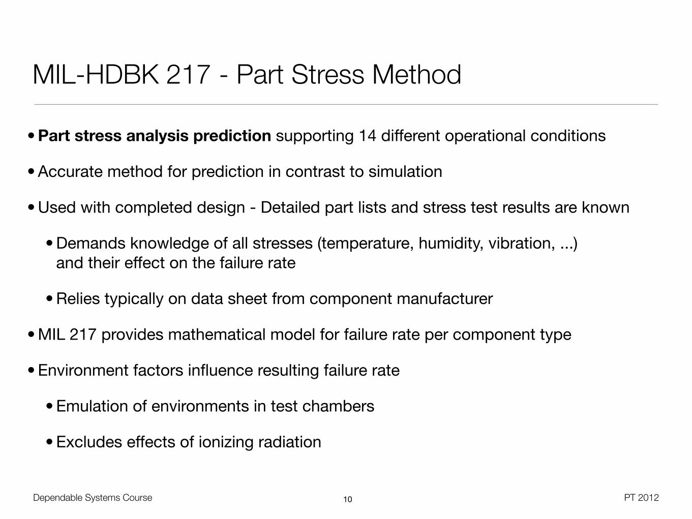
• Part stress analysis prediction supporting 14 different operational conditions

• Accurate method for prediction in contrast to simulation

• Used with completed design - Detailed part lists and stress test results are known

• Demands knowledge of all stresses (temperature, humidity, vibration, ...) and their effect on the failure rate

• Relies typically on data sheet from component manufacturer

• MIL 217 provides mathematical model for failure rate per component type

• Environment factors influence resulting failure rate

• Emulation of environments in test chambers

• Excludes effects of ionizing radiation


MIL-HDBK 217 - Part Stress Method

10

• Determine the system failiure rate from each part‘s stress level

• - Learning factor (1-2)

• - Production quality factor (1-100)

• - Temperature acceleration factor (1-100)

• - Voltage stress factor

• - Application environment factor (1-20)

• - Technology constants for complexity (1-100) and case (1-20)

• - Failure rate per million hours

• Supports quantitative assessment of relative cost-benefit of system-level tradeoffs


MIL-HDBK 217 - Part Stress Method

11

� = ⇥L⇥Q(C1⇥T⇥V + C2⇥E)

⇡L

⇡Q

⇡T

⇡V

⇡E

C1, C2

�


Application Environment Factor


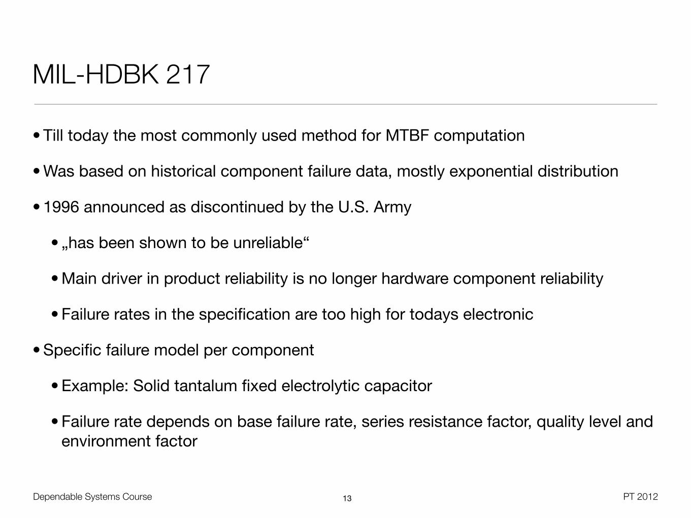
MIL-HDBK 217

• Till today the most commonly used method for MTBF computation

• Was based on historical component failure data, mostly exponential distribution

• 1996 announced as discontinued by the U.S. Army

• „has been shown to be unreliable“

• Main driver in product reliability is no longer hardware component reliability

• Failure rates in the specification are too high for todays electronic

• Specific failure model per component

• Example: Solid tantalum fixed electrolytic capacitor

• Failure rate depends on base failure rate, series resistance factor, quality level and environment factor

13


MIL-HDBK 217 Tool Support

14


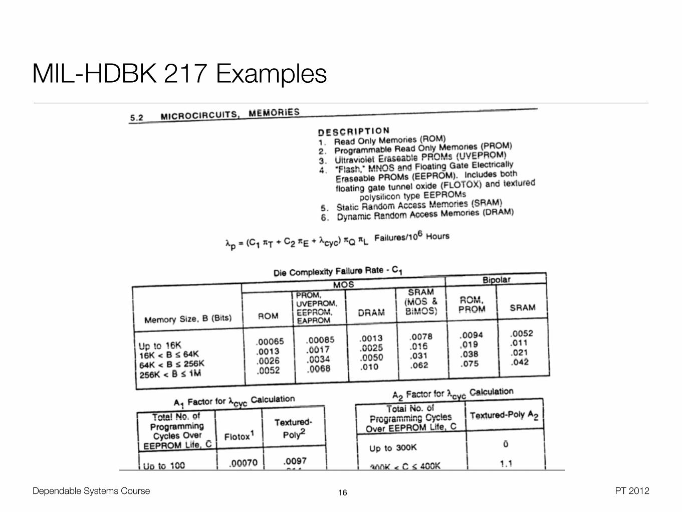
MIL-HDBK 217 Examples

15


MIL-HDBK 217 Examples

16


Mechanical Parts

17


Telcordia (Bellcore) SR-332 / TR-332

• Reliability prediction model evolved from telecom industry equipment experience

• First developed by Bellcore Communications research, based on MIL217

• Lower and more conservative values for MTBF

• Availability with relation to failures per billion component operation hours

• Factors: Static failure rate of basic component, quality, electrical load, temperature

• Often observed that calculations are more optimistic than in MIL 217

• Requires fewer parameters than MIL 217 - Four unified quality levels

• Different components supported - Printed circuit boards, lasers, tubes, magnetic memories (217) vs. gyroscopes, batteries, heaters, coolers, computer systems

18


Telcordia (Bellcore) SR-332 / TR-332

• Three methods with empirically proven data

• Method 1: Part count approach, no field data available

• Supports first year multiplier for infant mortality modeling

• Method 2: Method 1 extended with laboratory test data

• Supports Bayes weighting procedure for burn-in results

• Method 3: Method 2 including field failure tracking

• Different Bayes weighting based on the similarity of the field data components

19

� = ⇡g�b⇡S⇡t

Environmental Factor Base Failure Rate from

Transistor Count

Quality Factor

Temperature Factor, default 40 deg


MIL-HDBK-217 vs. Telecordia

• Often observed that Telecordia calculations are much more optimistic

• Telecordia requires fewer parameters for components, has additional capabilities for considering burn-in data, laboratory test data, and field data

• Helps to calculate failure rates based on historical data

• Can model infant mortality effects

• Telecordia uses Failures-In-Time (FIT) - per billion hours, MIL uses failures per million hours

• Operating environments in Telecordia are limited, since only designed for telco users

• Telecordia quality levels are simplified

20


PRISM

• PRISM released by Reliability Analysis Center (RAC) in 2000

• Can update predictions based on test data

• Adresses factors such as development process robustness and thermal cycling

• Basic consideration of system software part

• Seen as industry replacement for MIL 217

• Factors in the model: Initial failure rate, infant mortality, environment, design processes, reliability growth, manufacturing processes, item management processes, wear-out processes, software failure rate, ...

• Quantitative factors are determined through an interactive process

21


RIAC 217Plus

• Predictive models for integrated circuits (Hermetic and non-hermetic), diodes, transistors, capacitors, resistors and thyristors

• Based on over 2x1013 operation hours and 795,000 failures

• Includes also software model

• System level modeling part for non-component variables

• Failure rate contribution terms: Operating, non-operating, cycling, induced

• Process grading factors: Parts, Design, Manufacturing, System Management, Wear-out, Induced and No Defect Found

• Model degree of action for failure mitigation

• Still only series calculation, no active-parallel or standby redundancy support

22


Other Sources• IEC TR62380 - Technical report of the International Electrotechnical Commission,

considers thermical behaviour and system under different environmental conditions

• IEC 61709 - Parts count approach, every user relies on own failure rates

• NPRD-95 - Failure rates for > 25.000 mechanical and electromechanical parts, collected from 1970s till 1994

• HRD5 - Handbook for reliability data of electronic components used in Telco industry, developed by British Telecom, similar to MIL 217

• VZAP95 - Electrostatic discharge susceptibility for 22.000 devices (e.g. microcircuits)

• RDF 2000 - Different approach for failure rates

• Cycling profiles - power on/off, temperature cycling

• Demands complex information (e.g. thermal expansion, transistor technology, package related failure rates, working time ratio)

23


Other Sources

• WASH-1400 (NUREG-75/015) - „Reactor Safety Study - An Assessment of Accident Risks in U.S. Commercial Nuclear Power Plants“ 1975

• IEEE Standard 500

• Government-Industry Data Exchange Program (GIDEP)

• NUREG/CR-1278; „Handbook of Human Reliability Analysis with Emphasis on Nuclear Power Plant Applications;“ 1980

• SAE model - Society of automotive engineers, similar equations to MIL 217

• Modifying factors are are specific for automotive industry

• Examples: Component composition, ambient temperature, location in the vehicle

24


Failure Probability Sources (Clemens & Sverdrup)

• Original data

• Manufacturer‘s Data

• Industry Consensus Standards, MIL Standards

• Historical Evidence - Same or similar systems

• Similar product technique - Take experience from old product with similar attributes

• Similar complexity technique - Estimate reliability by relate product complexity to well-known product

• Prediction by function technique - Part count prediction or part stress prediction

• Simulation or testing

25


Comparison

• Naval Surface Warfare Center (NSWC) Crane Division established working group for modification factors of MIL 217

• Industry survey - Reliability prediction methods used

• From survey of 1900 component tests, less than 25% had used prediction models

• 38% of them used MIL 217

26(C)VMECritical.com


Software - A Different Story

27


Software Reliability Assessment

• Software bugs are permanent faults, but behave as transient faults

• Activation depends on software usage pattern and input values

• Timing effects with parallel or distributed execution

• Software aging effects

• Fraction of system failures reasoned by software increased in the last decades

• Possibilities for software reliability assessment

• Black box models - No details known, observations from testing or operation

• Reliability growth models

• Software metric models - Derive knowledge from static code properties

28


Dimensions of Black Box Models (Musa et al.)

29

Consider stress factors, e.g.

through aging

Consider infinite number of failures,

e.g. from reintroduced bugs

Consider how failures are distributed in time

Consider how failure severity is

distributed

Good for managers


Software Reliability Growth Models

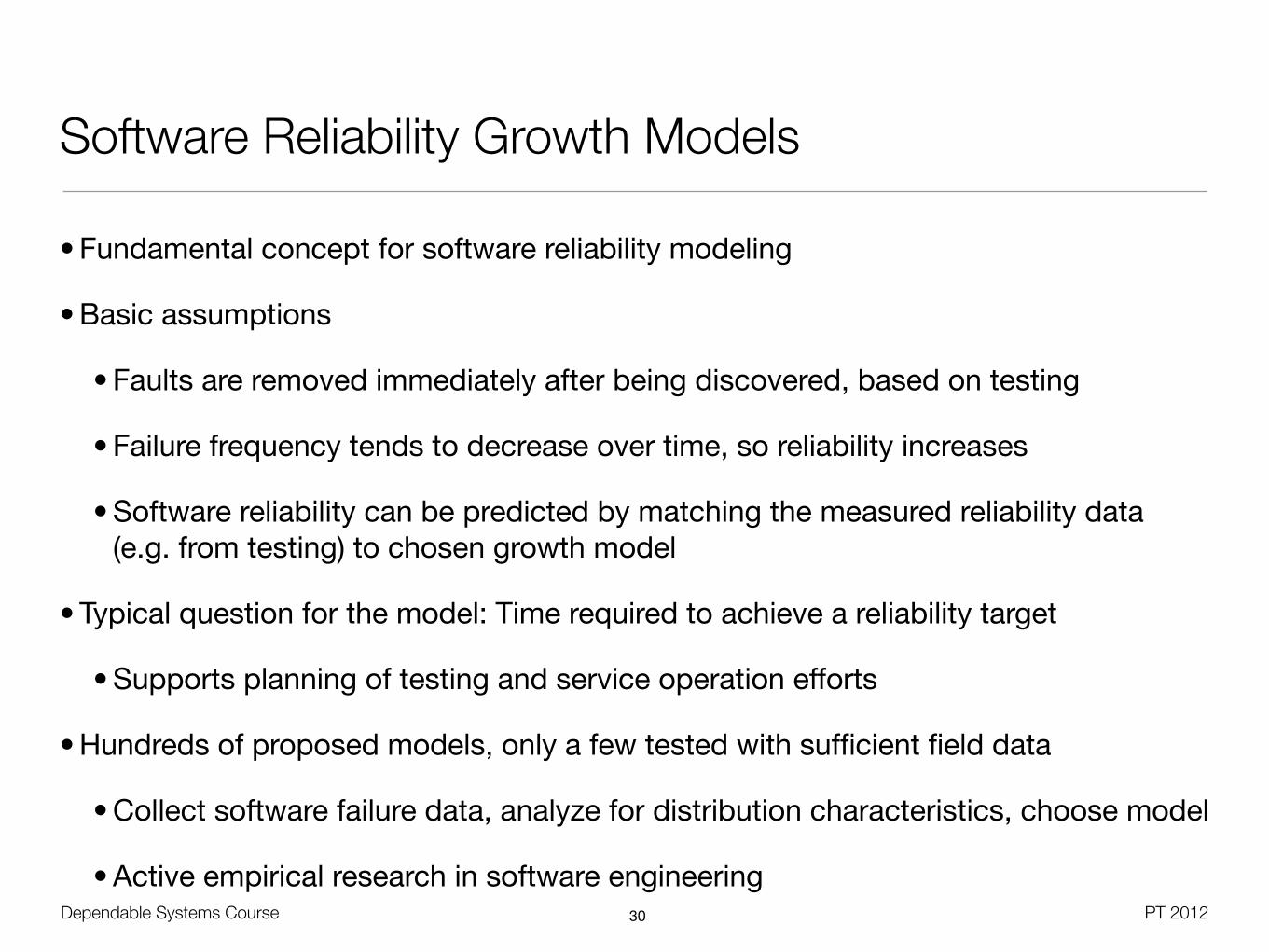
• Fundamental concept for software reliability modeling

• Basic assumptions

• Faults are removed immediately after being discovered, based on testing

• Failure frequency tends to decrease over time, so reliability increases

• Software reliability can be predicted by matching the measured reliability data (e.g. from testing) to chosen growth model

• Typical question for the model: Time required to achieve a reliability target

• Supports planning of testing and service operation efforts

• Hundreds of proposed models, only a few tested with sufficient field data

• Collect software failure data, analyze for distribution characteristics, choose model

• Active empirical research in software engineering30


Reliability Growth Model Analysis by Tandem [Wood]

31

• Concave models: Fault detection rate decreases over time with repair activities

• S-Shaped models: Early testing is more efficient than later testing

• Ramp-up phase were error detection rate increases

• Example: Early phase detects faults that prevent the application from running


Software Reliability Growth Models• Classification by Singpurwalla and Wilson (1994)

• Type I: Model time between successive failures

• Should get longer as faults are removed from the software

• Time is assumed to follow a function, related to number of non-fixed faults

• Type I-1: Based on failure rate (Example: Jelinski-Moranda Model (1972))

• Type I-2: Model inter-failure time based on previous inter-failure times

• Type II: Counting process to model the number of failures per time unit

• As faults are removed, observed number of failures per unit should decrease

• Typically derivation of remaining number of defects / failures

• Example: Basic execution time model by Musa (1984)

32

• Finite number of bugs, inter-failure time has exponential distribution

• Assumptions: Faults are equal, errors occur randomly and independent from each other, error detection rate is constant, repairs are perfect, repair time is negligible, software operation during test is the same as in production use

• Constant function for failure rate in the i-th time interval, based on constant factor and number of bugs:

• Estimation of : Number of failures in interval i / length of interval i

• Failure rate estimation based on testing efforts done so far

• Allows to reason about (remaining) number of dormant faults in the software


Jelinksi-Moranda Model

33

�i

�i = � ⇤Ni

• Time between failures 7.5 min before testing, 2h after testing

• 75 faults were removed

• Looking for number of initial faults and proportionality constant

• Reliability after 10h of operation with the improved version of the software


Example: Jelinski-Moranda

34

�0 = � ⇤N �end = � ⇤ (N � 75) �0 ⇡ 1

0, 125

�end ⇡ 1

2�0

�end=

N

N � 75= 16 N = 80,� = 0, 1

R(10h) = e��end10h = 7%R(ti) = e��iti


Basic Execution Time Model (Musa)• Another reliability growth model

• Determine cumulative number of failures by time i

• Start with estimated number of initial faults, get number of corrected fault after

• Fundamental assumption that correction of faults does not introduce new ones

• One of the first models to rely on execution time, instead of calendar time

• Resources limit execution time spent per unit calendar time

• Expression in terms of CPU time can indicate ,stress‘ on software

• Random process that represents the number of failures experienced by some time

• Exponential distribution of resulting failure intensity function

• Failure intensity changes with a constant rate, depending on the number of observed failures

35

⌧

• - Failure rate (number of failures per time unit)

• - Execution time (time since the program is running)

• - Mean number of expected failures in an execution time interval

• - Initial failure rate at the start of execution

• - Total number of failures over an infinite time period

• Assumed maximum number offailures leads to decreasingover time


Basic Execution Time Model (Musa)

36

µ(⌧) = ⌫0(1� e��0⌫0

⌧ )

�

�0

⌧

⌫0

µ

�(⌧) = �0e��0

⌫0⌧

µ⌫0



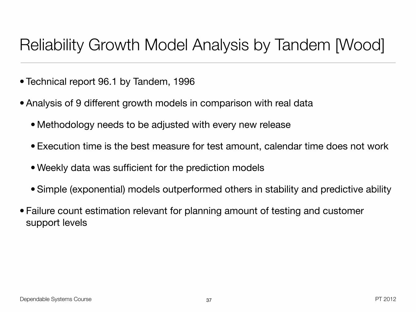
• Technical report 96.1 by Tandem, 1996

• Analysis of 9 different growth models in comparison with real data

• Methodology needs to be adjusted with every new release

• Execution time is the best measure for test amount, calendar time does not work

• Weekly data was sufficient for the prediction models

• Simple (exponential) models outperformed others in stability and predictive ability

• Failure count estimation relevant for planning amount of testing and customer support levels

37

• Reality check for typical assumptions

• „Repair is perfect“: New defects are less likely to be detected, since regression is not as comprehensive as the original tests

• „Each unit of time is equivalent“: Corner tests are more likely to find defects, test reruns for fixed bugs are less likely to find new defects

• „Tests represent operational profile“: Size and transaction volume of production system is typically not reproducible

• „Failures are independent“: Reasonable, except for badly tested portions of code

• During testing, the model should predict additional test effort for some quality level

• After test, the model should predict the number of remaining defects in production

• Most models do not become stable until about 60% of the tests



38



39

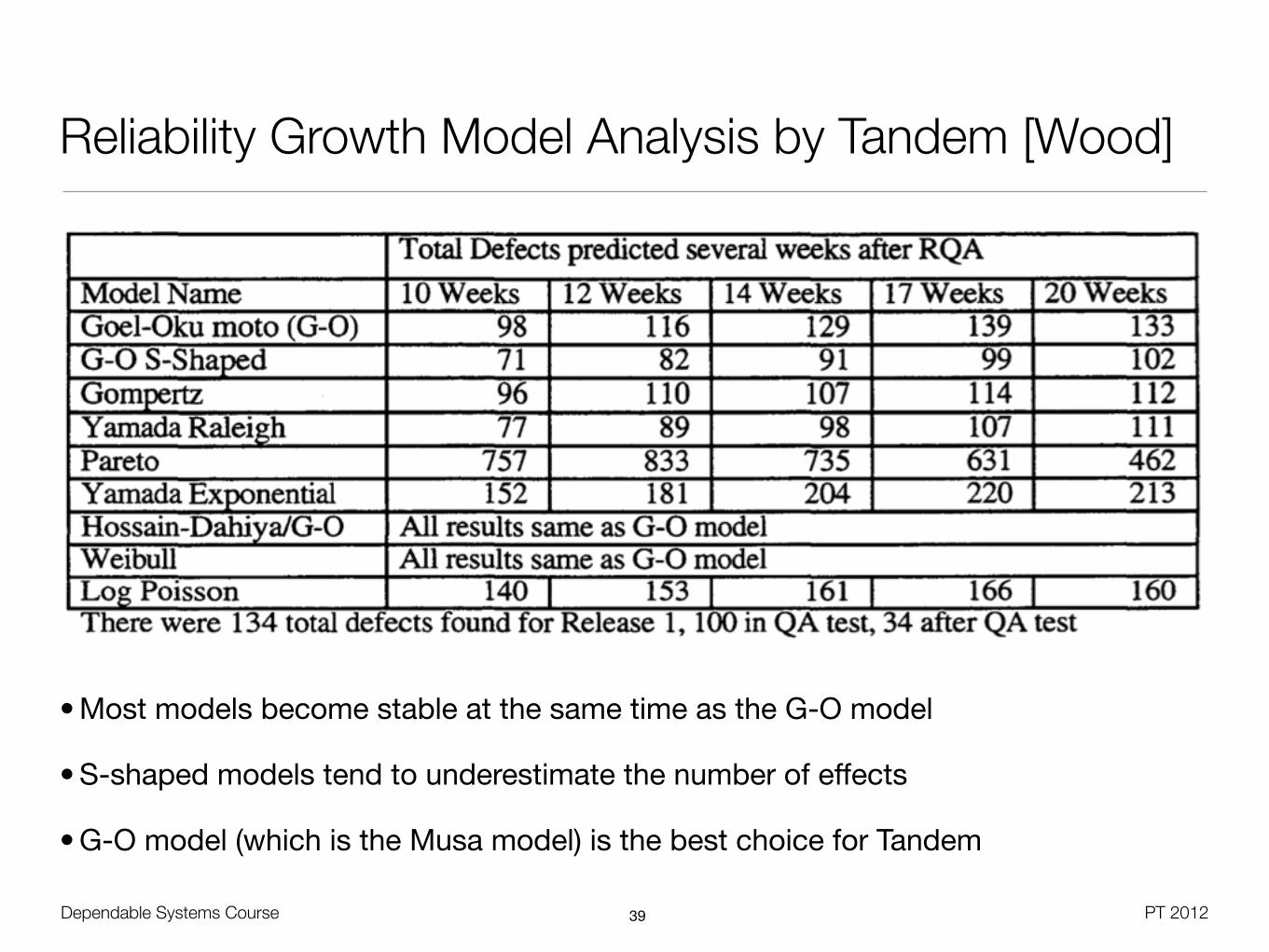
• Most models become stable at the same time as the G-O model

• S-shaped models tend to underestimate the number of effects

• G-O model (which is the Musa model) is the best choice for Tandem


White Box Approach - Software Metric Models

• Larger software is more complex, which brings more dormant faults

• Idea: Rank software reliability by complexity measures

• ... for the code itself

• ... for the development process

• Complexity metrics should rank degree of difficulty for design and implementation of program structures, algorithms, and communication schemes

• Hundreds of different metrics proposed, variety of software tools

• Most basic approach - lines of code (LOC)

• Industry standard from 0,3 to 2 bugs per 1000 lines of code

• Better data for structured analysis available with large open source projects

40

41

2010

2011

2012


Example: CyVis Tool for Java


Halstead Metric• Statistical approach - Complexity is related to number of operators and operands

• Only defined on method level, OO code analysis must consider additional structure

• Program length N = Number of operators NOP + total number of operands NOD

• Vocabulary size n = Number of unique operators nOP + number of unique operands nOD

• Program volume V = N * log2(n)

• Describes size of an implementation by vocabulary and (mainly) by program length

• In-place changes are ok ...

• Difficulty level D = (nOP / 2) * (NOD / nOD), program level L = 1 / D

• Error proneness is proportional to number of unique operators -> since most languages only offer a few, this should be small

• Also proportional to the level of operand reuse through the code45

x = x + 1;NOP=nOP=3

NOD=3nOD=2


Halstead Metric• Effort to implement / understand the program E = V * D

• Depends on volume and difficulty level of the analyzed software

• Describes mental effort to re-create the software (only implementation)

• Questioned by some researchers

• Time in seconds to implement / understand the program T = E / 18

• Stroud number 18 by John Stroud, psychologist

• -> humans can detect between 5 and 20 discrete events per second

• Widely ignored in software metric tools

• Number of delivered bugs B = V / 3000

• Bug count correlates with the complexity / effort to understand the software

• Statistically proven for object-oriented software46


Cyclomatic Complexity

47

Thomas McCabe‘s cyclomatic complexity (1976)

• Measure based on graph representation of the control flow

• Cyclomatic number v(G) for a strongly connected graph:

• Number of directed edges - number of vertexes + number of connected components

• Expresses number of independent conditional paths in the control flow

• No consideration of data structure complexity, data flow, or module interface design

• Goal should be max. 15 for functions, 100 for files

• Studies showed correlation between fault count andcyclomatic number

if / for /

while / case / catch /

....

Phantom edge for strongly connected graph


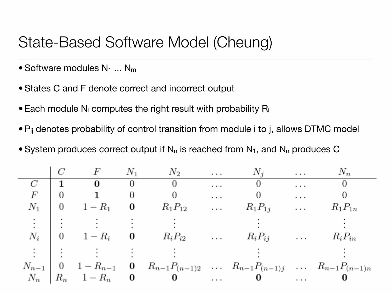
State-Based Software Model (Cheung)• Software modules N1 ... Nm

• States C and F denote correct and incorrect output

• Each module Ni computes the right result with probability Ri

• Pij denotes probability of control transition from module i to j, allows DTMC model

• System produces correct output if Nn is reached from N1, and Nn produces C

48

49

"All Models are Wrong - Some are Useful." George E. P. Box

reliability prediction - operating systems and middleware group

Documents