Relocation of the Rich: Migration in Response to TopTax Rate Changes from Spanish Reforms

David R. Agrawal, University of Kentucky and CESifoDirk Foremny, Universitat de Barcelona and IEB

Skilled workers play a vital role in the �scal systems of advancedeconomies, and may easily be �worth their weight in gold�, bringing

�scal dividends of substantial size to the societies in which they reside.� David Wildasin (2009)

Research Agenda

How sensitive are the �rich� to interstate tax di�erentials?

Are individuals in certain industries and occupations more sensitive?

How large are the revenue implications of tax-induced migration?

Ideal context to study migration:

I A reform implemented in 2011 granted Spanish regions the ability toset their own income tax rates and brackets.

I Tax rates diverged substantially across regions.

Motivation to Study Migration

High-income individuals are potentially very responsive to taxdi�erentials, especially within a country when mobility barriers are low.

Mobility is a form of behavioral response.

I Moving increases the e�ciency cost of taxation and limitsredistribution policy (Mirrlees 1982: optimal degree of redistributionwill decline as the mobility elasticity increases).

I Mobile labor may induce ine�cient tax competition (Wildasin 2006;Wilson 2009).

Substantially discussed in the media and policy world: e.g., �ActorDepardieu bids 'adieu' to France to avoid taxes.�

Tax-Induced Migration: An Example

Academic Evidence

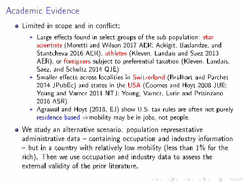
Limited in scope and in con�ict:

I Large e�ects found in select groups of the sub-population: starscientists (Moretti and Wilson 2017 AER; Ackigit, Baslandze, andStantcheva 2016 AER), athletes (Kleven, Landais and Saez 2013AER), or foreigners subject to preferential taxation (Kleven, Landais,Saez, and Schultz 2014 QJE)

I Smaller e�ects across localities in Switzerland (Brülhart and Parchet2014 JPubEc) and states in the USA (Coomes and Hoyt 2008 JUE;Young and Varner 2011 NTJ; Young, Varner, Lurie and Prisinzano2016 ASR)

I Agrawal and Hoyt (2018, EJ) show U.S. tax rules are often not purelyresidence based ⇒mobility may be in jobs, not people.

We study an alternative scenario: population representativeadministrative data � containing occupation and industry information� but in a country with relatively low mobility (less than 1% for therich). Then we use occupation and industry data to assess theexternal validity of the prior literature.

Main Contributions and Findings

Graphical evidence on aggregate e�ects using stocks.

I Clear e�ect after accounting for origin and destination �xed e�ects.I But, the elasticity of the stock has relatively small revenue implications.

Choice model: movers are more likely to select low-tax states.

I The Madrid - Catalunya tax di�erential increases probability of movingto Madrid by 2.25 points.

I Heterogeneity by various occupations/industries.

Interpretation of the elasticities using a simple theoretical model.

I Tax decreases result in revenue losses suggesting the mechanical e�ectof the tax change outweighs the behavioral response.

Preview of Results

−.0

6−

.04

−.0

20

.02

.04

.06

Pro

babi

lity

of M

ovin

g to

Reg

ion

−.03 −.02 −.01 0 .01 .02 .03log net−of−mtr

Pre−Reform

−.0

6−

.04

−.0

20

.02

.04

.06

Pro

babi

lity

of M

ovin

g to

Reg

ion

−.03 −.02 −.01 0 .01 .02 .03log net−of−mtr

Post−Reform

pre-reform: no e�ect post-reform: �large� e�ect

Institutional Details

Institutional Details: Reform

Spain consists of 17 autonomous communities (in Spanish:comunidades autónomas).

Since the 90s regions are entitled to receive a share of the PersonalIncome Tax (Impuesto sobre la Renta de las Personas Físicas), wherewe study the labor income tax bases.

I Capital income is taxed under a single federal tax system.

A major wave of decentralization in 2011 had substantial changes:

I The share of revenue that regions could keep.I The authority to change the tax rates / tax brackets were given to theregions.

Immediately following the new law, the regions began changing taxrates substantially, but mainly at the top portion of the incomedistribution.

Spanish Popular Press: �Fiscal Paradise�

Tax Changes (2011)

-20

24

mtr

rela

tive

to c

entra

l mtr

in p

erce

ntag

e po

ints

0 100 200 300income in thousands of Euros

AND ARA AST BAL

CAN CAN CAL CAM

CAT VAL EXD GAL

MAD MUR RIO

2011

Tax Changes (2012)

-20

24

mtr

rela

tive

to c

entra

l mtr

in p

erce

ntag

e po

ints

0 100 200 300income in thousands of Euros

AND ARA AST BAL

CAN CAN CAL CAM

CAT VAL EXD GAL

MAD MUR RIO

2012

Tax Changes (2013)

-20

24

mtr

rela

tive

to c

entra

l mtr

in p

erce

ntag

e po

ints

0 100 200 300income in thousands of Euros

AND ARA AST BAL

CAN CAN CAL CAM

CAT VAL EXD GAL

MAD MUR RIO

2013

Tax Changes (2014)

-20

24

mtr

rela

tive

to c

entra

l mtr

in p

erce

ntag

e po

ints

0 100 200 300income in thousands of Euros

AND ARA AST BAL

CAN CAN CAL CAM

CAT VAL EXD GAL

MAD MUR RIO

2014

Tax Declaration

Tax Rates and Income Distribution: 2014

[Calculator]

Data

Spain's Continuous Sample of Employment Histories (MuestraContinua de Vidas Laborales, MCVL)

I Data matches individual microdata from from social security recordswith data from the tax administration (Agencia Tributaria, AEAT ),and o�cial population register data (Padrón Continuo) from theSpanish National Statistical O�ce (INE ).

I A 4% non-strati�ed random sample (over 1 million observations eachyear) of the population of individuals which had any relationship withSpain's Social Security system in a given year.

Income tax data not top coded: ideal for high-income.I We create an income variable which is the sum of all reported incomeby di�erent employers within each year which is subject to the personalincome tax (labor income, self employed income, etc.).

We de�ne a change of location if an individual changed his or herresidence using o�cial population registers.

I Information is taken from the o�cial register of the municipality wherepeople registered (for local services).

Tax Rates

The data only includes income reported by employers or self-employed,not full tax declarations.

NBER's TAXSIM does not exist for Spain � we digitize Spain's taxcode.

We write a tax calculator where we simulate average and marginal taxrates for each individual in each year for each region and reconstructthe taxes of all individuals included in the data.

I This simulation takes into account the variation of marginal tax rates,their brackets, and basic deductions and tax credits for children, elderly,and disabilities.

Method I: Aggregate AnalysisEstimation of Location Equilibrium Condition

Theoretical Motivation

Let the utility of a top income individual living in region r in period tbe given by:

Vr ,t = α ln(cr ,t) + π ln(gr ,t) + µr − γ ln(Nr ,t) (1)

I where cr ,t = (1− τr ,t)wr ,t and ln(Nr ,t) is a disutility (congestion)function.

If production is given by ArNθr ,tK

ϑr we must have wr ,t = Ar K

ϑr

Nθr ,t

.

Then, the equilibrium between regions r = {d , o} is characterized by

ln(Nd ,t

No,t) =

1

θ + γ

α

ln

(1− τd ,t

1− τo,t

)+

π

α(θ + γ

α)ln

(gd ,tgo,t

)+ ζd −ζo (2)

I where ζr depends on time-invariant parameters µr , Ar and Kr .I Adjustment of wages:

dln(wr ,t )dln(1−τr ,t ) =

dln(Nr ,t )dln(1−τr ,t ) ×

dln(wr ,t )dln(Nr ,t ) =−θ

1

θ+γ

α

Aggregate Analysis: Stocks

ln(Ndt/Not)︸ ︷︷ ︸stock ratio

= β [ln(1−atrdt)− ln(1−atrot)]︸ ︷︷ ︸tax differentials

+ ζd︸︷︷︸’d’ amenities

+ ζo︸︷︷︸’o’ amenitiess

+ζt +δ ln

(gd ,tgo,t

)+Xodtφ +νodt

(3)

The left hand side variable ln(Ndt/Not) is the log of the stock ofindividuals in the top 1% of the income distribution in region drelative to region o.

Need to address potential taxable income responses. Do so byfocusing on individuals that repeat being in the top 1%.

The stock elasticity with respect to the net of tax top rate is

approximately equal to β =dln(Nd ,t)

dln(1−atrd ,t) −dln(No,t)

dln(1−atrd ,t) .

Model Motivation

Model leads to a structural interpretation of estimated coe�cient:

I β is the e�ect of tax changes including through their indirect e�ect onregional wages, i.e. the e�ect taking all �xed regional characteristics(amenities) and public services as given except for taxes and wages.

Visual Results: Stock Elasticity

theory: ↓tax di�erential =⇒ ↑ net of tax di�erential =⇒↑ stock of rich

Results : Stock Elasticity

Baseline Speci�cations AddressingTaxableIncome

ATR (1) ATR (2) MTR (3) ATR (4) MTR (5)

ln[(1−atrd)/(1−atro)] 0.917* 1.116** 0.656** 0.878* 0.556**(0.537) (0.545) (0.300) (0.500) (0.267)

Government Spending? Y Y Y Y YFE? Y Y Y Y Y

Controls? N Y Y Y YNumber of Observations 1050 1050 1050 1050 1050

Visual Results : Lower Parts of Distribution

Visual Results : Pre-reform Stock & Post-reform Taxes

Event Study

Method II: Individual AnalysisWhere to Move?

Individual Choice Model [Estimation]

Letting j index location and (i , t) index a particular move, we estimateusing movers pre-reform (2005-2010) and post-reform (2011-2014):

di ,t,j = β ln(1− τi ,t,j )︸ ︷︷ ︸tax differentials

+ ζjxi ,t︸ ︷︷ ︸wage differentials

+ γzi ,t,j︸ ︷︷ ︸moving costs

+

region-year effects︷︸︸︷ιt,j + αi ,t︸︷︷︸

case FE

+εi ,t,j

(4)

with di ,t,j = 1 if selected region and 0 otherwise.

Identi�cation: Taxes

Approach A:

I Because counterfactual wages are not observed, calculation of thecounterfactual average tax rate presents challenges if wages are notsimilar across regions.

I Initially use the marginal tax rate of individual i . Independent ofearnings if income changes across regions do not induce tax bracketchanges across regions.

Approach B:

I Also calculate the average tax rate assuming that wages are constantacross regions.

I Individuals are more likely to select states with high wages =⇒overestimate counterfactual wages =⇒ overestimate counterfactualaverage tax rates (progressive).

I Resolved using an IV approach.

Identi�cation: Wage Di�erentials

But, we also need to control for wages across other regions. To dothis, we construct measures of �ability� using education, male, age,and age squared.

I We then interact these variables with state dummy variables to allowfor di�erent e�ects across states.

I This allows the returns to education and the skill premium of age tovary by region.

Identi�cation: Other Policies / Amenities

We control for other policy changes and amenities across regions.

I We do this by including region by year �xed e�ects to capture anyalternative speci�c policies that may vary over time.

I Implicitly assumes all policies are constant across individuals within aregion.

I Public services consumption likely similar in the top 1%.

Identi�cation: Moving Costs

We control for moving costs.

I Calculate the distance between all alternatives and the region of origin(gravity model of migration).

I Dummy variable for region of birth.I Dummy variable for region of �rst job.I Dummy variable for region moving from.I Dummy variable for region of �rm headquarters.

Sample Selection

We focus on movers.

Because movers are a very small share of the population, it is likelythat the equilibrium tax rates selected following the �scaldecentralization are driven by the large share of the stayers � reducingendogeneity concerns (Brulhart, Bucovetsky and Schmidheiny 2015).

Schmidheiny (2006): �Households do not daily decide upon their placeof residence. There are speci�c moments in any individual's life [�rstjob, family changes, career opportunities] when the decision aboutwhere to live becomes urgent.... Limiting the analysis to movinghouseholds therefore eliminates the bias when including householdsthat stay in a per se sub-optimal location because of high monetaryand psychological costs of moving. However, the limitation to movinghouseholds introduces a potential selection bias when the unobservedindividual factors that trigger the decision to move are correlated withthe unobserved individual taste for certain locations.�

Sample Selection

Address these concerns by:

I Testing for di�erences in covariates between movers and stayers.I Estimate the model for the full sample of stayers and movers (smaller,but same sign).

Results: MTR

(1) (2) (3)

ln(1−mtri ,j ,t) 0.569 0.604** 0.677**(0.367) (0.305) (0.308)

place of origin -0.797*** -0.766***(0.061) (0.060)

place of birth 0.207*** 0.206***(0.022) (0.021)

place of �rst work 0.186*** 0.177***(0.020) (0.020)

work place 0.288*** 0.261***(0.018) (0.021)

ln(distance) -0.075*** -0.072***(0.009) (0.009)

individual �xed e�ects Y Y Yj by year �xed e�ects Y Y Y

j by education N N Yj by age N N Y

j by age squared N N Yj by male N N Y

observations 13,395 13,395 13,395

Results: ATR

(1) (2) (3)

ln(1−atri ,j ,t) 0.588 0.714** 0.904***(0.420) (0.343) (0.332)

place of origin -0.797*** -0.766***(0.061) (0.060)

place of birth 0.207*** 0.206***(0.022) (0.021)

place of �rst work 0.185*** 0.177***(0.020) (0.020)

work place 0.288*** 0.261***(0.018) (0.021)

ln(distance) -0.075*** -0.072***(0.009) (0.009)

individual �xed e�ects Y Y Yj by year �xed e�ects Y Y Y

j by education N N Yj by age N N Y

j by age squared N N Yj by male N N Y

observations 13,395 13,395 13,395

Results: ATR with IV(1) (2) (3)

ln(1−atri ,j ,t) 1.452 1.542* 1.731**(0.948) (0.788) (0.797)

place of origin -0.797*** -0.766***(0.061) (0.060)

place of birth 0.207*** 0.206***(0.022) (0.021)

place of �rst work 0.185*** 0.177***(0.020) (0.020)

work place 0.288*** 0.261***(0.018) (0.021)

ln(distance) -0.075*** -0.072***(0.009) (0.009)

individual �xed e�ects Y Y Yj by year �xed e�ects Y Y Y

j by education N N Yj by age N N Y

j by age squared N N Yj by male N N Y

observations 13,395 13,395 13,395

First Stage Coe�cient 0.392*** 0.392*** 0.391***(0.015) (0.014) (0.014)

F-statistic 735.1 740.2 792.9

Magnitudes

E�ect of Madrid-Catalunya average tax di�erential (0.75 points in2013)

I increases probability of moving to Madrid by 2.25 percentage points.

E�ect of Madrid's tax cut in 2014 (0.4 points)

I Further increases probability of moving to Madrid by another 1.15points.

Results: IV Fixed Bracket

Exclude observations 1, 2.5 and 5% above/below cut-o�s.

Idea: reduces the possibility that the instrument is in�uenced bycounterfactual income.

(1) (2) (3)1%

above/below2.5%above/below

5%above/below

ln(1−atri ,j ,t) 1.782** 1.864** 3.734***(0.896) (0.871) (1.277)

observations 12,255 10,620 8,040

Placebo Test: Do Post-reform Rates Predict Pre-reformMigration?

(1) (2) (3) (4)MTR ATR MTR ATR

Pre-Reform Post-Reform

ln(1− τ) 0.038 0.093 0.866*** 2.051***(0.194) (0.469) (0.281) (0.687)

observations 6,180 6,180 4,965 4,965

Discussion

Real response vs. tax evasion

I The top 1% may have the ability to change residence to a second homewithout spending the majority of the year there.

I From a tax revenue perspective real response and tax evasion are bothimportant.

A tax professional we spoke to: recommends his clients to 'move'when income is above 80,000 euros.

We conduct heterogeneity analysis to try to determine the mechanism.

Heterogeneity of E�ect

Individual characteristics:

I Younger than 40 ( 1.680*) vs. older than 40 (1.759**)I Kids (1.767*) vs. no kids (1.709**).I University degree (2.185**) vs. no degree (1.008).I Men (1.483) vs. women (3.012***).

Job characteristics:

I Not �red (2.015**) vs. �red (0.847).I No contract change (1.660**) vs. contract change (2.429**).

Occupation/Industry

The prior literature has been unable to answer the question whetherpolicymakers can take the estimates derived for star scientists andathletes and apply these elasticities to the top of the incomedistribution more generally.

The Spanish data we have access to has occupation and industryreported in the data.

This section also helps to inform the recent policy debate on thee�ciency of tax schemes for top earners in speci�c occupations.Several OECD countries have preferential tax schemes for foreigners incertain high-income occupations.

Major contribution: prior literature focusing on star scientists andathletes masks substantial heterogeneity by otheroccupations/industries.

Occupation

self-employed

engineers, college graduates

managers and graduate assistants

others

-2 0 2 4 6

effects by occupation

Industry

HealthOther

Real EstateInformation

FinancialProfessional/Scientific

ConstructionEducation

Wholesale/RetailExtraterritorial Activities

ManufacturingTransportation

Arts/EntertainmentAdministrative

AgricultureTourism

Electricity-10 -5 0 5 10

effects by industry

Interpretation of Magnitudes

Magnitudes

To interpret, we construct a simple model of tax revenue maximizationfrom the rich.

Then a top tax rate change above income y will have mechanical andbehavioral e�ects:

dR = [N(y − y)]dτ︸ ︷︷ ︸mechanical

−εa

[N(y − y)

τ

1− τ

]dτ︸ ︷︷ ︸

taxable income

−ηN(y − y)

[T (y)

y −T (y)

]dτ︸ ︷︷ ︸

mobility

ETI for governments that hits the La�er Curve Peak:

ε =1−η

(T (y)

y−T (y)

)a(

τ

1−τ

) .

Revenue Changes / La�er Tax Rates

We calculate the change in revenue relative to what would have beenobtained if the region had simply mimicked the federal government taxrate.

I Focus on a τ applied to income above 94,000 euros (top 1%).I We estimate the Pareto parameter (we estimate this for each region).I Elasticity of taxable income is taken from Saez, Slemrod and Giertz(2012, JEL). We take the midpoint of the literature (0.25) and adjustit downward slightly because of the smaller number of deductions inSpain (consistent with our estimates).

Use the parametric bootstrap to construct con�dence bands.

Revenue E�ects

-.5 0 .5 1 1.5percent of revenue

La RiojaMurciaMadridGalicia

ExtremaduraValencia

CatalunyaCastilla la Mancha

Castilla y LeonCantabriaCanarias

Islas BalearsAsturiaAragon

Andalusia

mechanical taxable incomemobility

What Does the ETI Need to Be to Break Even?0

.25

.5.7

51

1.25

1.5

elas

ticity

of t

axab

le in

com

e

Andalu

sia

Aragon

Asturia

Islas

Bale

ars

Canari

as

Cantab

ria

Castill

a y Le

on

Castill

a la M

anch

a

Catalun

ya

Valenc

ia

Extrem

adura

Galicia

Madrid

Murcia

La R

ioja

-.03

-.02

-.01

0.0

1.0

2.0

3lo

g sh

are

of in

com

e to

the

top

1%

-.04 -.02 0 .02 .04log net of tax rate

Conclusion

State taxes have a signi�cant and stable e�ect on the locationdecisions of the rich, but the revenue implications appear to be small.

Thus, we �nd short-run evidence consistent with Epple and Romer(1991) that shows local redistribution is feasible even with migration.

In the long-run, this may create substantial sorting e�ects as migration�ows persist, in particular when avoidance is easy.

I Mobility is likely to rise over time given demographic shifts andtechnological innovations, which may in turn impose added constraintson the ability to engage in redistributive �scal policy (Wildasin 2015).

Within Variation[Back]

0.5

11.

5w

ithin

sta

ndar

d de

viat

ion

2004 2006 2008 2010 2012 2014year

Top 1% Top 2%Top 3%

Aggregate Analysis: Flows [Back]

ln(Podt/Poot) = e[ln(1−mtrdt)− ln(1−mtrot)]+ζo +ζd +ζt +Xodtβ +νodt

(5)

The left hand side variable ln(Podt/Poot) is the log odds ratio wherePodt is the the share of the population that moves from state o tostate d in year t and Poot is the fraction of the population that staysin state o in the same year.

ε is the approximate �ow elasticity with respect to the net of tax rate.

Visual Results: Flow Model

theory: ↓tax di�erential =⇒ ↑ net of tax di�erential =⇒↑ odds of moving

Estimation [Back]

For ease of notation, we prove this for an equation with a singlecovariate denoted by xi ,t,j , the sum of the predicted probabilities for agiven move (i , t) from our regression is given by

∑j (βxi ,t,j + αi ,t) = ∑j βxi ,t,j + ∑j αi ,t = β ·J ·xi ,t +J · αi ,t = J · [βxi ,t + αi ,t ](6)

where the upper-bar denotes an average over the j 's. Given we have Jalternative regions and, for a given move, only one region can bechosen:

d i ,t =1

J. (7)

As shown in Greene (2003), the linear model implies that theestimated �xed e�ects, αi ,t , are given by

αi ,t = d i ,t − βx i ,t ⇒ d i ,t = βx i ,t + αi ,t . (8)

Algebra proves that ∑j(βxi ,t,j + αi ) = J ·d i ,t = J · 1J = 1. This, then,necessarily implies that an increase in the probability of selecting oneregion must lower the probability of the alternative regions.