report documentation page · report documentation page the public reporting burden for...
TRANSCRIPT

AFRL-SR-AR-TR-09-0051
REPORT DOCUMENTATION PAGE
The public reporting burden for th^^Tllection of information is estimated to average 1 hour per response, including the time for reviewing instructions, searching existing data sources, gathering and maintaining the data needed, and completing and reviewing the collection of information. Send comments regarding this burden estimate or any other aspect of this collection of information, including suggestions for reducing the burden, to Department of Defense, Washington Headquarters Services, Directorate for Information Operations and Reports (0704-0188), 1215 Jefferson Davis Highway, Suite 1204, Arlington, VA 22202-4302. Respondents should be aware that notwithstanding any other provision of law, no person shall be subject to any penalty for failing to comply with a collection of information if it does not display a currently valid 0MB control number,
PLEASE DO NOT RETURN YOUR FORM TO THE ABOVE ADDRESS.
1. REPORT DATE (DD-MM-YYYY)
06-02-2009 REPORT TYPE
Final Performance Report 3. DATES COVERED (From - To)
01-01-2006 to 30-11-2008 4. TITLE AND SUBTITLE
Advanced Steganographic and Digital Forensic Methods
5a. CONTRACT NUMBER
FA9559-06-1-0046
5b. GRANT NUMBER
5c. PROGRAM ELEMENT NUMBER
6. AUTHOR(S)
Dr. Jessica Fridrich
5d. PROJECT NUMBER
5e. TASK NUMBER
5f. WORK UNIT NUMBER
7. PERFORMING ORGANIZATION NAME(S) AND ADDRESS(ES)
The Research Foundation of State University of New York SUNY at Binghamton 4400 Vestal Parkway East Binghamton, NY 13902-6000
8. PERFORMING ORGANIZATION REPORT NUMBER
9. SPONSORING/MONITORING AGENCY NAME(S) AND ADDRESS(ES)
USAF, AFRL AF Office of Scientific Research 875 N. Randolph Street RM 3112
rlington.VA / / / ,
10. SPONSOR/MONITOR'S ACRONYM(S)
AFOSR/PKA
— _^rlin; 11. SPONSOR/MONITOR'S REPORT
NUMBER(S)
12. DISTRIBUTION/AVAILABIL/TY STATEMENT
All data delivered is approved for public release; distribution is unlimited.
13. SUPPLEMENTARY NOTES
14. ABSTRACT
The author developed and advanced a new class of digital forensic techniques to verify origin and integrity of digital imagery based on systematic artifacts of imaging sensors called photo-response non-uniformity (PRNU), which is caused by slight variations in physical dimensions of pixels and inhomogeneity of silicon. PRNU thus forms a unique fingerprint that characterizes an imaging device, such as a camera, camcorder, or scanner. Both CCD and CMOS technologies exhibit this type of irregularity. The specific achievements include perfecting the methodology for estimating the fingerprint from images, extending to cases when the image under investigation is simultaneously cropped, scaled, and processed, extending the technology when the digital image is printed, developing technology capable of determining the camera model from the fingerprint, and a large scale validation on millions of images from 6900 cameras of 150 models. The techniques have dual purpose and are important for information validation in military intelligence gathering, law enforcement, and forensic investigation.
15. SUBJECT TERMS
Digital Forensics, sensor, fingerprint, identification, forgery detection, authentication, information assurance, media security
16. SECURITY CLASSIFICATION OF:
a. REPORT
Unclassified
b. ABSTRACT
Unclassified
c. THIS PAGE
Unclassified
17. LIMITATION OF ABSTRACT
Unlimited
18. NUMBER OF PAGES
43
19a. NAME OF RESPONSIBLE PERSON
Jessica Fridrich
19b. TELEPHONE NUMBER (Include area code!
607 777 6177 Standard Form 298 (Rev. 8/98) Prescribed by ANSI Std Z39 18

Final Report
Effort title: Advanced Digital Forensic and Steganalysis Methods
Principal Investigator: Jessica Fridrich, Professor Department of Electrical and Computer Engineering Binghamton University T. J. Watson School Binghamton, NY 13902-6000 Ph: 607-777-6177, Fax: 607-777-4464
Agreement Number: FA95500610046
20090324145

OBJECTIVES
1. Develop new digital forensic methods for identifying camera from images or video clips.
2. Develop digital forensic methods for detection and localization of tampering. 3. Implement the methods in Matlab and deliver the code to US Air Force and FBI. 1. Assist in technology transfer to law enforcement and government.
PERSONNEL SUPPORTED
Dr. Jessica Fridrich, PI Dr. Miroslav Goljan, Postdoctoral Assistant Dr. Mo Chen, Postdoctoral Assistant Mr. Tomas Filler, PhD student Dr. Paul Blythe, DDE Lab Manager
LIST OF PUBLISHED PAPERS AND DISSERTATIONS
1. J. Lukas, J. Fridrich, and M. Goljan: "Digital Camera Identification from Sensor Pattern Noise." IEEE Transactions on Information Security and Forensics, vol. 1(2), pp. 205-214, June 2006.
2. M. Goljan and J. Fridrich: "Camera Identification from Cropped and Scaled Images." Proc. SPIE Electronic Imaging, Forensics, Security, Steganography, and Watermarking of Multimedia Contents X, vol. 6819, San Jose, California, January 28 - 30, pp. 0E-1-0E-13 2008.
3. M. Goljan and J. Fridrich: "Camera Identification from Printed Images." Proc. SPIE Electronic Imaging, Forensics, Security, Steganography, and Watermarking of Multimedia Contents X, vol. 6819, San Jose, California, January 28 - 30, pp. 01-1-01-12,2008.
4. M. Goljan, Mo Chen, and J. Fridrich: "Identifying Common Source Digital Camera from Image Pairs." Proc. IEEE ICIP 07, San Antonio, TX, 2007.
5. Mo Chen, J. Fridrich, and M. Goljan: "Source Digital Camcorder Identification Using CCD Photo Response Non-uniformity." Proc. SPIE Electronic Imaging, Security, Steganography, and Watermarking of Multimedia Contents IX, vol. 6505, San Jose, California, January 28 - February 1, pp. 1G-1H, 2007.
6. J. Fridrich, Mo Chen, M. Goljan, and J. Lukas, "Digital Imaging Sensor Identification (Further Study)." Proc. SPIE, Electronic Imaging, Security, Steganography, and Watermarking of Multimedia Contents IX, vol. 6505, San Jose, CA, January 28-February 2, pp. 0P-0Q, 2007.
7. Lukas, J., Fridrich, J., and Goljan, M.: "Detecting Digital Image Forgeries Using Sensor Pattern Noise." Proc. SPIE, Electronic Imaging, Security, Steganography, and Watermarking of Multimedia Contents VIII, vol. 6072. San Jose, California, pp. 0Y1-0Y11,2006.
8. Mo Chen, J. Fridrich, M. Goljan, and J. Lukas: "Determining Image Origin and Integrity Using Sensor Noise." IEEE Transactions on Information Security and Forensics, vol. 1(1), pp. 74-90, March 2008.

9. J. Fridrich, Mo Chen, J. Lukas, and M. Goljan, "Imaging Sensor Noise as Digital X-Ray for Revealing Forgeries." 9' Information Hiding Workshop, Saint Malo, France, June 9-11, LNCS, 4567, Springer-Verlag, pp. 342-358, 2007.
10. T. Filler, J. Fridrich, and M. Goljan: "Using Sensor Pattern Noise for Camera Model Identification." Proc. IEEE ICIP 08, San Diego, CA, September 2008
11. J. Fridrich, "Digital Image Forensics using Sensor Noise," to appear in Special Issue Signal processing Magazine, 2009 (to appear).
12. M. Goljan, J. Fridrich, and T. Filler: "Camera Identification - Large Scale Test." Proc. SPIE, Electronic Imaging, Security and Forensics of Multimedia Contents XI, San Jose, CA, January 18-22, 2009 (to appear).
All papers were presented at the above noted conferences or published in respective journals.
PhD Dissertations
J. Lukas: Digital Image Forensics using Sensor Pattern Noise, Ph.D. Dissertation, SUNY Binghamton, Department of Electrical and Computer Engineering, June 2006.
INTERACTIONS/TRANSITIONS
The research findings were presented to peers at professional meetings, such as the Annual AFOSR PI meetings, IEEE International Conference on Image Processing (ICIP) in San Antonio, Texas, in September 2007, IEEE International Conference on Image Processing (ICIP) in San Diego, California, in September 2008, 9th Information Hiding Workshop in 2007, and multiple times at SPIE Electronic Imaging in San Jose in January 2006-2009. The research was also briefed to FBI forensic investigators and to AFRL in July 2008.
The PI and the co-PI, Miroslav Goljan, provided expert service to Scottish law enforcement agency in connection with a child pornography case. The issue was whether a given image was taken with the exact same camera as other images. For the first time, the camera ID technology has been used in the court of law.
The research results are continuously being incorporated into a software application through a separate project "FIND Camera" funded by the FBI. This application is intended to be used by forensic investigators for fighting crime and collecting intelligence as part of Homeland Security
PATENTS
The achievements on this project are closely related to two patents that were previously filed. Below are included the patent disclosures.
PROJECT: RB-218 (internal Research Foundation filing number)

TITLE: METHOD AND APPARATUS FOR IDENTIFYING AN IMAGING DEVICE
INVENTORS: Jessica Fridrich, Miroslav Goljan, Jan Lukas
DESCRIPTION
This invention concerns the problem of authenticating digital images. In particular, the method enables to decisively answer the following questions: Given a digital image and the imaging device that took it, was some specific area of the image tampered? Is there a tampered area in the image and where?
As digital images and video continue to replace their analog counterparts, reliable and inexpensive authentication of digital images increases on importance. It would especially prove useful in the court. For example, the integrity verification could be used for establishing the authenticity of images presented as evidence, or, in a child pornography case, one could prove that certain imagery, or at least its critical part, has been obtained using a specific camera and is not a computer-generated image.
The process of image authentication has been approached from several different directions, but to the best of our knowledge none so far led to a generally usable reliable method. The technology in this disclosure uses as an identification pattern a certain component of the pattern noise of imaging sensors (e.g., CCD or CMOS) caused by pixel non-uniformity. This pattern is extracted using a specially designed denoising filter. The presence of the pattern in a given region of interest is established using a mathematical operation called correlation. This approach is computationally simple and relatively reliable. It is also possible to verify integrity of processed images (e.g., using JPEG or other common processing operations).
TECHNOLOGY APPLICATIONS
1. Discovering digital forgeries 2. Establishing integrity of digital images
TECHNOLOGY ADVANTAGES
1. Reliability and accuracy of this technology unmatched by other competing methods
2. Simplicity and computational efficiency 3. Applicability to all sensor types and image acquisition devices
PROJECT: RB-222 (internal Research Foundation filing number)
TITLE: USING PATTERN NOISE OF IMAGING SENSORS FOR IMAGING HARDWARE IDENTIFICATION

INVENTORS: Jessica Fridrich, Miroslav Goljan, Jan Lukas
DESCRIPTION
This patent concerns the problem of identification of the imaging digital device (e.g., a digital camera or scanner) from a digital image. In particular, the method enables to decisively answer the following questions: Given a digital camera, was a specific image taken with that camera (or scanned with a given scanner)? Did the same camera take two images?
As digital images and video continue to replace their analog counterparts, reliable, inexpensive, and fast identification of digital image origin increases on importance. It would especially prove useful in the court. For example, the identification could be used for establishing the origin of images presented as evidence, or, in a child pornography case, one could prove that certain imagery has been obtained using a specific camera and is not a computer-generated image.
The process of image identification has been approached from several different directions, but to the best of our knowledge none so far led to a reliable method. The technology in this disclosure uses as an identification pattern a certain component of the pattern noise of imaging sensors (e.g., CCD or CMOS) caused by pixel non-uniformity. This pattern is extracted using a specially designed denoising filter. The presence of the pattern in a given image is established using a mathematical operation called correlation. This approach is computationally simple and is able to distinguish between cameras of the exact same model. It is also possible to identify the camera from processed images (e.g., using JPEG or other common processing operations).
TECNOLOGY APPLICATIONS
1. Determining the origin of digital images 2. Matching an image to a camera
TECHNOLOGY ADVANTAGES
1. Reliability and accuracy of this technology unmatched by other competing methods
2. Simplicity and computational efficiency 3. Applicability to all sensor types and image acquisition devices 4. Ability to distinguish between cameras of the exact same brand
POTENTIAL LICENSEES (for both patents)
Law enforcement and forensic analysts, Government contractors and consulting companies, imaging companies and companies manufacturing imaging sensors, companies dealing with data embedding and security, such as Digimarc (http//www.digimarc.com), Verance (http://www.verance.com/). Blue Spike, Inc.

(http://www.bluespike.com), Signum Technologies, (http://www.sianumtech.com), or Wetstone, Inc. (http://www.wetstonestech.com).
COMPETING PRODUCTS: None known at this time.
STAGE OF DEVELOPMENT: A working prototype is available for demonstration.
STATUS OF INTELLECTUAL PROPERTY PROTECTION: U.S. patent applications submitted in 2006.
RIGHTS AVAILABLE: Due to the potential broad applicability of the technology, non- exclusive licensing and distribution is anticipated.
CONTACT FOR FURTHER INFORMATION:
Dr. Eugene B. Krentsel Director, Technology Transfer and Innovation Partnerships Division of Research P.O. Box 6000 State University of New York Binghamton, NY 13902-6000 Phone: 607-777-5871 Fax: 607-777-4354 E-mail: [email protected]

Advanced Digital Forensics and Steganalysis Methods
Executive Summary
Despite its unquestionable advantages, it is highly non-trivial to establish integrity and origin of digitally represented visual data. This issue of trust increases on importance with widespread use of digital imagery for reconnaissance, remote sensing, intelligence gathering, command, control, and communication. Digital images and video are also increasingly more often produced as silent witness in court in connection with child pornography and movie piracy cases, or insurance claims.
The goal of digital forensics is to investigate the origin, integrity, and meaning of evidence in digital form. The fundamental tasks of digital forensic can be clustered into the following six types:
Source Classification with the objective to assign a given image to several broad classes based on then- origin, such as scan vs. digital camera, or Canon vs. Kodak.
Device Identification focuses on proving that a given image was obtained by a specific device that is available (prove that a given camera took a certain image or video).
Device Linking, whose task is to group images according to their common source. For example, given a set of images, we would like to find out which images were obtained using the exact same camera.
Processing History Recovery with the objective to recover the processing chain applied to a given image. Here, we are interested in non-malicious processing, e.g., lossy compression, filtering, recoloring, contrast/brightness adjustment, etc.
Integrity Verification or forgery detection is a procedure aimed at discovering malicious processing, such as object removal or adding.
Anomaly Investigation deals with explaining anomalies found in images that may be a product of digital processing or other phenomena specific to digital cameras.
The research presented in this report concerns virtually all of the above forensic tasks. The crucial idea is to use pixel imperfections of digital imaging sensors as a unique fingerprint whose form, integrity, or presence can be used to reach high-certainty conclusions about image processing history, integrity, and origin. The sensor fingerprint is an intrinsic property of all digital imaging sensors due to slight variations among individual pixels in their ability to convert photons to electrons. Consequently, every sensor casts a weak noise-like pattern onto every image it takes. This pattern, or a sensor fingerprint, is essentially an unintentional stochastic spread-spectrum watermark that survives processing, such as lossy compression or filtering. This report explains in detail how this fingerprint can be estimated from images taken by the camera and later detected in a given image to establish image origin and integrity. Extensive experimental evaluation confirms the usability of the proposed methods in practice.
All forensic techniques developed under this project have been peer reviewed and published. The methods were also implemented in Matlab, tested, and made available to the US Government. A forensic software product with all reported methods is currently being developed by PAR, Inc., for use by the FBI and US Air Force. The technology is covered by two US patents.

1. MAIN ACHIEVEMENTS
In this section, the investigator summarizes the main research achievements. Some topics are then detailed in individual sections, while the remaining material uncovered in this report is cited with appropriate references.
1.1 INTRODUCTION
There exist two types of imaging sensors commonly found in digital cameras, camcorders, and scanners—CCD (Charge-Coupled Device) and CMOS (Complementary Metal-Oxide Semiconductor). Both consist of a large number of photo detectors also called pixels. Pixels are made of silicon and capture light by converting photons into electrons using the photoelectric effect. The accumulated charge is transferred out of the sensor, amplified, and then converted to a digital signal in an AD converter and further processed before the data is stored in an image format, such as JPEG.
The pixels are usually rectangular, several microns across. The amount of electrons generated by the incident light at a pixel depends on the physical dimensions of the pixel photosensitive area and on the homogeneity of silicon. The pixels' physical dimensions slightly vary due to imperfections in the manufacturing process. Also, the inhomogeneity naturally present in silicon contributes to variations in quantum efficiency among pixels (the ability to convert photons to electrons). The differences among pixels can be captured with a matrix K of the same dimensions as the sensor. When the imaging sensor is illuminated with ideally uniform light intensity Y, in the absence of other noise sources, the sensor would register a noise-like signal Y+YK instead. The term YK is usually referred to as the pixel-to-pixel non- uniformity or PRNU.
The matrix K is responsible for a major part of what is called the camera fingerprint. The fingerprint can be estimated experimentally, for example by taking many images of a uniformly illuminated surface and averaging the images to isolate the systematic component of all images. At the same time, the averaging suppresses random noise components, such as the shot noise (random variations in the number of photons reaching the pixel caused by quantum properties of light) or the readout noise (random noise introduced during the sensor readout), etc [1,2]. Fig. 1 shows a magnified portion of a fingerprint from a 4 megapixel Canon G2 camera obtained by averaging 120 8-bit grayscale images with average grayscale 128 across each image. Bright dots correspond to pixels that consistently generate more electrons, while dark dots mark pixels whose response is consistently lower. The variance in pixel values across the averaged image (before adjusting its range for visualization) was 0.5 or 51 dB. Although the strength of the fingerprint strongly depends on the camera model, the sensor fingerprint is typically quite a weak signal.
Fig. 1: Magnified portion of the sensor fingerprint from Canon G2. The dynamic range was scaled to the interval [0,255] for visualization.
Fig. 2 shows the magnitude of the Fourier transform of one pixel row in the averaged image. The signal resembles white noise with an attenuated high frequency band.

Besides the PRNU, the camera fingerprint essentially contains all systematic defects of the sensor, including hot and dead pixels (pixels that consistently produce high and low output independently of illumination) and the so called dark current (a noise-like pattern that the camera would take with its objective covered). The most important component of the fingerprint is the PRNU. The PRNU term KK is only weakly present in dark areas where K«0. Also, completely saturated areas of an image, where the pixels were filled to their full capacity, producing a constant signal, do not carry any traces of PRNU or any other noise for that matter.
It should be noted that essentially all imaging sensors (CCD, CMOS, JFET, or CMOS-Foveon• X3) are built from semiconductors and their manufacturing techniques are similar. Therefore, these sensors will likely exhibit fingerprints with similar properties.
400 600 800 Frequency
Fig. 2: Magnitude of Fourier transform of one row of the sensor fingerprint.
Even though the PRNU term is stochastic in nature, it is a relatively stable component of the sensor over its life span. The factor K is thus a very useful forensic quantity responsible for a unique sensor fingerprint with the following important properties:
1. Dimensionality. The fingerprint is stochastic in nature and has a large information content, which makes it unique to each sensor.
2. Universality. All imaging sensors exhibit PRNU.
3. Generality. The fingerprint is present in every picture independently of the camera optics, camera settings, or scene content, with the exception of completely dark images.
4. Stability. It is stable in time and under wide range of environmental conditions (temperature, humidity).
5. Robustness. It survives lossy compression, filtering, gamma correction, and many other typical processing.
The fingerprint can be used for many forensic tasks:
• By testing the presence of a specific fingerprint in the image, one can achieve reliable device identification (e.g., prove that a certain camera took a given image) or prove that two images were taken by the same device (device linking). The presence of camera fingerprint in an image is also indicative of the fact that the image under investigation is natural and not a computer rendering.
• By establishing the absence of the fingerprint in individual image regions, it is possible to discover maliciously replaced parts of the image. This task pertains to integrity verification.
• By detecting the strength or form of the fingerprint, it is possible to reconstruct some of the processing history. For example, one can use the fingerprint as a template to estimate geometrical processing, such as scaling, cropping, or rotation. Non-geometrical operations are also going to influence the strength of the fingerprint in the image and thus can be potentially detected.
• The spectral and spatial characteristics of the fingerprint can be used to identify the camera model or distinguish between a scan and a digital camera image (the scan will exhibit spatial anisotropy).

This section is organized as follows. In Section 1.2, the author describes a simplified sensor output model and uses it to derive a maximum likelihood estimator for the fingerprint. At the same time, the author points out the need to preprocess the estimated signal to remove certain systematic patterns that might increase false alarms in device identification and missed detections when using the fingerprint for image integrity verification. Starting again with the sensor model in Section 1.3, the task of detecting the PRNU is formulated as a two-channel problem and approached using the generalized likelihood ratio test in Neyman-Pearson setting. First, the detector for device identification is derived and then adapted for device linking and fingerprint matching. Section 1.4 shows how the fingerprint can be used for integrity verification by detecting the fingerprint in individual image blocks. The reliability of camera identification and forgery detection using sensor fingerprint is illustrated on real imagery in Section 1.5.
Everywhere in this report, boldface font will denote vectors (or matrices) of length specified in the text, e.g., X and Y are vectors of length n and X[i] denotes the rth component of X. Sometimes, pixels will be indexed using a two-dimensional index formed by the row and column index. Unless mentioned otherwise, all operations among vectors or matrices, such as product, ratio, raising to a power, etc., are elementwisc.
The dot product of vectors is denoted as XD Y = 2_, X[z']Y[/'] with ||X||=vXD X being the L2 norm of
X. Denoting the sample mean with a bar, the normalized correlation is
corr{X,\) =
1.2 SENSOR EINGERPRINT ESTIMATION
(X-X)D (Y-Y)
IIX-XIHIY-YII
The PRNU is injected into the image during acquisition before the signal is quantized or processed in any other manner. In order to derive an estimator of the fingerprint, we need to formulate a model of the sensor output.
1.2.1 Sensor Output Model
Even though the process of acquiring a digital image is quite complex and varies greatly across different camera models, some basic elements are common to most cameras. The light cast by the camera optics is projected onto the pixel grid of the imaging sensor. The charge generated through interaction of photons with silicon is amplified and quantized. Then, the signal from each color channel is adjusted for gain (scaled) to achieve proper white balance. Because most sensors cannot register color, the pixels are typically equipped with a color filter that lets only light of one specific color (red, green, or blue) enter the pixel. The array of filters is called the color filter array (CFA). To obtain a color image, the signal is interpolated or demosaicked. Finally, the colors are further adjusted to correctly display on a computer monitor through color correction and gamma correction. Cameras may also employ filtering, such as denoising or sharpening. At the very end of this processing chain, the image is stored in the JPEG or some other format, which may involve quantization.
Let us denote by I[i] the quantized signal registered at pixel i, / = 1, ..., mxn, before demosaicking. Here, mxn are image dimensions. Let Y[i] be the incident light intensity at pixel i. Dropping the pixel indices for better readability, the following vector form of the sensor output model is used
I = g''[(l + K)Y + ftf+Q. (1)
All operations in (1) (and everywhere else in this report) are element-wise. In (1), g is the gain factor (different for each color channel) and /is the gamma correction factor (typically, y*a 0.45). The matrix K is a zero-mean noise-like signal responsible for the PRNU (the sensor fingerprint). Denoted by 12 is a combination of the other noise sources, such as the dark current, shot noise, and read-out noise [2]; Q is the combined distortion due to quantization and/or JPEG compression.

In parts of the image that are not dark, the dominant term in the square bracket in (1) is the scene light intensity Y. By factoring it out and keeping the first two terms in the Taylor expansion of (1 + x)r= 1 + yx + O(x') at x = 0, one obtains
[ = (gYy-[l + K + ft/Yj+QD
(g\y • (I+ yK + yil/\)+ Q = l{0) + t0)K+ 0.
In (2), I'0' = igYY denotes the ideal sensor output in the absence of any noise or imperfections. Note that
I(l),K is the PRNU term and 0 = yVa)\/Y + & is the modeling noise. In the last expression in (2), the
scalar factor y was absorbed into the PRNU factor K to simplify the notation.
1.2.2 Sensor Fingerprint Estimation
The sensor output model is now used to derive an estimator of the PRNU factor K. A good introductory text on signal estimation and detection is [3,4].
The SNR between the signal of interest I(0)K and observed data I can be improved by suppressing the
noiseless image I(0) by subtracting from both sides of (2) a denoised version of I, I'01 = F(l), obtained using a denoising filter F (Section 1.6 describes the filter used in all experiments in this report):
W = I -1(0) = IK +1(0) - il0) + (I(0) - I)K + 0
= IK + E .
It is easier to estimate the PRNU term from W than from I because the filter suppresses the image content. Here, S is the sum of 0 and two additional terms introduced by the denoising filter.
It will be assumed that a database of d > 1 images, Ij, ..., I,/, obtained by the camera, is available. For each pixel i, the sequence E,[f], ..., E(/[i] is modeled as white Gaussian noise (WGN) with variance <J~. Even
though the noise term is technically not independent of the PRNU signal IK due to the term (I10' -I)K ,
because the energy of this term is small compared to IK, the assumption that E is independent of IK is reasonable.
From (3), one can write for each A' = 1, ..., d
f = KA Wt=I,-i<°\i<0)=F(It). (4)
Under the assumption about the noise term the log-likelihood of observing W, l\k given K is
L(K) = -^±log{2^f(lkf)-±(^^-K/ . (5)
2 *_• *,i 2cr /(It)
By taking partial derivatives of (5) with respect to individual elements of K and solving for K, one obtains the maximum likelihood estimate K
y wi sjm = fyjkiik-K = Q^k=h_Ll, (6)
5K tt v2'(lkY y^y
The Cramer-Rao Lower Bound (CRLB) gives the bound on the variance of K

d2L(K) t(U2 . , *=l —s \'/ir(K\ ^
a2
dK2
-E d2L(K)
dK2 t(I,): (7)
Because the sensor model (3) is linear, the CRLB says that the maximum likelihood estimator is minimum
variance unbiased and its variance var(K) ~ \ld. From (7), one can see that the best images for estimation
of K are those with high luminance (but not saturated) and small <j~ (which means smooth content). If the camera under investigation is in our possession, out-of-focus images of bright cloudy sky would be the best. In practice, good estimates of the fingerprint may be obtained from 20-50 natural images depending on the camera. If sky images are used instead of natural images, only approximately one half of them would be enough to obtain an estimate of the same accuracy.
The estimate K contains all components that are systematically present in every image, including artifacts introduced by color interpolation, JPEG compression, on-sensor signal transfer [5], and sensor design. While the PRNU is unique to the sensor, the other artifacts are shared among cameras of the same model or sensor design. Consequently, PRNU factors estimated from two different cameras may be slightly correlated, which undesirably increases the false identification rate. Fortunately, the artifacts manifest
themselves mainly as periodic signals in row and column averages of K and can be suppressed simply by
subtracting the averages from each row and column. For a PRNU estimate K with /;; rows and /; columns, the processing is described using the following pseudo-code
r(=l/nX;,K[U]
for/= 1 to/n {K'[i,j] = K[i,j]-rl foij= 1, ...,«}
c,.=l/m£" ,£•[*,;]
for / = 1 to n {K"[(,./] = K'[;, /'] - c, for / = 1, ..., m}.
The difference K-K" is called the linear pattern (see Fig. 3) and it is a useful forensic entity by itself- it can be used to classify a camera fingerprint to a camera model or brand. More details of this preprocessing step are contained in [6,28].
Fig. 3: Detail of the linear pattern for Canon S40.
To avoid cluttering the text with too many symbols, in the rest of this report, the processed fingerprint K"
will be denoted with the same symbol K .
For color images, the PRNU factor can be estimated for each color channel separately, obtaining thus three
fingerprints of the same dimensions KR, KG , and Kg. Since these three fingerprints are highly correlated due to in-camera processing, in all forensic methods in this report, before analyzing a color image under investigation it is converted to grayscale and correspondingly the three fingerprints are combined into one fingerprint using the usual conversion from RGB to grayscale
K = 0.2989K/(+0.587kc+0.114k;j. (8)

1.3 CAMERA IDENTIFICATION USING SENSOR FINGERPRINT
This section introduces general methodology for determining the origin of images or video using sensor fingerprint. The author starts with what is generally considered as the most frequently occurring situation in practice, which is camera identification from images. Here, the task is to determine if an image under investigation was taken with a given camera. This is achieved by testing whether the image noise residual contains the camera fingerprint. Anticipating the next two closely related forensic tasks, the author formulates the hypothesis testing problem for camera identification in a setting that is general enough to essentially cover the remaining tasks, which are device linking and fingerprint matching. In device linking, two images are tested if they came from the same camera (the camera itself may not be available). The task of matching two estimated fingerprints occurs in matching two video-clips because individual video frames from each clip can be used as a sequence of images from which an estimate of the camcorder fingerprint can be obtained (here, again, the cameras/camcorders may not be available to the analyst).
1.3.1 Device identification
A general scenario will be considered here, in which the image under investigation has possibly undergone a geometrical transformation, such as scaling or rotation. Let us assume that before applying any geometrical transformation the image was in grayscale represented with an mxn matrix l[i,j], i = 1, ... m, j - 1, ..., n. Let us denote as u the (unknown) vector of parameters describing the geometrical transformation, Tu. For example, u could be a scaling ratio or a two-dimensional vector consisting of the scaling parameter and unknown angle of rotation. In device identification, we wish to determine whether or not the transformed image
z=r„(i)
was taken with a camera with a known fingerprint estimate K . Thus, one can assume that the geometrical transformation is downgrading (such as downsampling) and thus it will be more advantageous to match the
inverse transform Tu~'(Z) with the fingerprint rather than matching Z with a downgraded version of K .
The detection problem will now be formulated in a slightly more general form to cover all three forensic tasks mentioned above within one framework. The fingerprint detection is the following two-channel hypothesis testing problem
H0: K. ^ K, ('))
H,: K. - K,
where
W, =I,K, +H, (10)
ru-(W2) = 7'11-'(Z)K2+E2.
In (10), all signals are observed with the exception of the noise terms E,, S, and the fingerprints K| and
K:. Specifically, for the device identification problem, I, =1, W, = K estimated in the previous section,
and H, is the estimation error of the PRNU. K, is the PRNU from the camera that took the image, W2 is
the geometrically transformed noise residual, and E, is a noise term. In general, u is an unknown
parameter. Note that since Tu '(W,) and W, may have different dimensions, the formulation (10) involves an unknown spatial shift between both signals, s.
Modeling the noise terms E, and E, as white Gaussian noise with known variances oy, a';, the generalized likelihood ratio test for this two-channel problem was derived in [7]. The test statistics is a sum of three terms: two energy-like quantities and a cross-correlation term

t = max{£,(u,s) + £2(u,s) + C(u,s)}, (11) u.s
zrtusnY i.['../'](w,[/+^Py+^])2
' ' t!,ofif[i,7]+ff,V(?,.",(Z)[''+*i.y'+*2])2
£ (u s) = y (ru'(Z)[/ + ^,y+^])2(7'u-'(W2)[/ + 5l,y + 52]):
2 ' f; c722(ru-
1(Z)ti+51)y + s2])2+a2Vlf['.i]
C(us) =yI,['\7lWJi,7](ru-,(Z)[i + J,,j+J2])(7;-|(W,)[i + Jpj + A-,])
tT a]X[i,j] + af(Tu-'(Z)[i + st,j + s2])2
The complexity of evaluating these three expressions is proportional to the square of the number of pixels, (mxn)~, which makes this detector unusable in practice. Thus, this detector is simplified to a normalized cross-correlation (NCC) that can be evaluated using fast Fourier transform. Under H,, the maximum in (11) is mainly due to the contribution of the cross-correlation term, C(u, s), that exhibits a sharp peak for the proper values of the geometrical transformation. Thus, a much faster suboptimal detector is the NCC between X and Y maximized over all shifts S[,s2, and u
m n
££(X[t,/]-X)(Y[* + 5I,/ + *2]-Y) NCC[J,,v,;u] = ^ 1, zziiij =, , (12)
|X-X||Y-Y|
which we view as an wxn matrix parameterized by u, where
i,w, y_ rB-'(Z)rM-'(w2) (13)
oflf + of(r.-'(Z))a Joft+o>(Tu-\Z))
A more stable detection statistics, whose meaning will become apparent from error analysis later in this section, that is strongly advocated to use for all camera identification tasks, is the Peak to Correlation Energy measure (PCE) defined as
NCC[s ,;u]2
PCE(u) = pejk , (14) —— - Y NCC[s;u]2
mn-15V | sj^
where for each fixed u, iVis a small region surrounding the peak value of NCC speak across all shifts s\, .v2.
For device identification from a single image, the fingerprint estimation noise E, is much weaker
compared to S2 for the noise residual of the image under investigation. Thus, CT2 = var(H,) D var(E,) = al
and (12) can be further simplified to a NCC between
X = W,=K and Y = 7,u"
1(Z)7,/'(W2).
Recall that I| = 1 for device identification when its fingerprint is known.
In practice, the maximum PCE value can be found by a search on a grid obtained by discretizing the range of u. Because the statistics is noise-like for incorrect values of u_and only exhibits a sharp peak in a small neighborhood of the correct value of u, unfortunately, gradient methods do not apply and one is left with a potentially expensive grid search. The grid has to be sufficiently dense in order not to miss the peak. As an example, the author now provides additional details how one can cany out the search when u = /• is an unknown scaling ratio. More details are given in Section 2.

0.6 0 7 0 8 0 9 1 scaling ratio
Fig. 4: Top: Detected peak in PCE(/-,). Bottom: Visual representation of the detected cropping and scaling parameters rpcak. Speak- The gray frame shows the original image size, while the black frame shows the image size after cropping before resizing.
Assuming the image under investigation has dimensions A/x/V, one searches for the scaling parameter at discrete values /•, < 1, i = 0, 1, ..., R, from r0 = 1 (no scaling, just cropping) down to rmin = max{A//w, Nln) < 1
r, =• 1
1 + 0.005/ '=0,1,2, (15)
For a fixed scaling parameter r„ the cross-correlation (12) does not have to be computed for all shifts s but
only for those that move the upsampled image Tr~\Z) within the dimensions of K because only such
shifts can be generated by cropping. Given that the dimensions of the upsampled image Tr '(Z) are M/r, x
N/rh one has the following range for the spatial shift s = (su s2)
0 < s, < m - M/r, and 0 < s2 < n - Nlrt. (16)
The peak of the two-dimensional NCC across all spatial shifts s is evaluated for each r, using PCE(/,) (14). If max, PCE(/-,) > r, the decision is H| (camera and image are matched). Moreover, the value of the scaling parameter at which the PCE attains this maximum determines the scaling ratio ;"peak. The location of the peak speak in the normalized cross-correlation determines the cropping parameters. Thus, as a by-product of this algorithm, one can determine the processing history of the image under investigation (see Fig. 4). The fingerprint can thus play the role of a synchronizing template similar to templates used in digital watermarking. It can also be used for reverse-engineering in-camera processing, such as digital zoom [9],
In any forensic application, it is important to keep the false alarm rate low. For camera identification tasks, this means that the probability, PFA, that a camera that did not take the image is falsely identified must be below a certain user-defined threshold (Neyman-Pearson setting). Thus, it is necessary to obtain a relationship between PFA and the threshold on the PCE. Note that the threshold will depend on the size of the search space, which is in turn determined by the dimensions of the image under investigation.
Under hypothesis H0 for a fixed scaling ratio rt, the values of the normalized cross-correlation NCC[s; /•,] as a function of s are well-modeled as white Gaussian noise <^") - N(0,a~) (see Fig. 5) with variance that

may depend on i. Estimating the variance of the Gaussian model using the sample variance ff: of
NCC[s; r,] over s after excluding a small central region Wsurrounding the peak
1 c, =
mn-13V | tM3t
-(0
I NCC[s;/-]2 (17)
one can now calculate the probability/?, that C, would attain the peak value NCC[speak; /peak] or larger by
chance:
/>•
NCCJi J
1 dx =
|«ak 'r]iaA I m a. i i
<W JPCEP. Una.
dx = Q peak
VPCIW
where Q(.v) = 1 - <t{x) with (P(x) denoting the cumulative distribution function of a standard normal variable /V(0,1) and PCEp<:ak = PCE(rpcak). As explained above, during the search for the cropping vector s, one only needs to search in the range (16), which means that the maximum is taken over &,= (m - Mir, + l)x(n - N/r,+ 1) samples of £'\ Thus, the probability that the maximum value of £" would not
exceed NCC[speak; rpeak] is (l - p])'. After R steps in the search, the probability of false alarm is
p^^-m-p.f (18)
Since the search can be stopped after the PCE reaches a certain threshold, it must be r, < ;-pt.ak. Because &:
is non-decreasing in /, cr^ I at > 1. Because Q(x) is decreasing, p, < Q\JPCEpak 1= p . Thus, because A-, <
mn, one obtains an upper bound on PFA
PnZl-il-pf-, (19)
where knax = V^ is the maximal number of values of the parameters /• and s over which the maximum of
(II) could be taken. Equation (19), together with/> = £>(Vr 1, determines the threshold for PCE, r= r
(PFA, M, N, m, n).
0
-2
-4
A -6 o o Z -8 •I
# -1° o
-12
-14
•15
# • NCC
Gaussian distribution
'••.
1 !i 3 3.5
x103
Fig. 5: Log-tail plot for the right tail of the sample distribution of NCC[s; r,] for an unmatched case.
This finishes the technical formulation and solution of the camera identification algorithm from a single image if the camera fingerprint is known. To demonstrate how reliable this algorithm is. Section 1.5 shows the results of experiments on real images. This algorithm can be used with small modifications for the other

two forensic tasks formulated in the beginning of this section, which are device linking and fingerprint matching.
Pseudo-code for camera identitlcation from cropped and scaled images
1. Read True color image Z, with M rows and N columns of pixels.
PCEpeak = 0; K is the estimated PRNU with m rows and n columns. 2. Set rmin = raa.x{M/m, Nln)
r = (r0, rur,,...,rmin), rt=————•, i = 0,1,2,. ..,R-l; 1 + 0.005;
r {detection threshold for PCE for a given PfA (see Equation (18) in Section 1.3.1)}
3. Extract noise W from Z in each color channel and combine the matrices using the linear transform (8): W = 0.2989 x WR + 0.5870 x WG + 0.1140 x WB.
4. Convert Z to grayscale. 5. For i = (R-3,R-2,R-l,0, 1, ...,R-4)
begin {phase 1 ( 6. Up-sample noise W by factor 1/r, to obtain 7j r (W) (nearest neighbor algorithm used).
7. Calculate the NCC matrix (12) with X = K and Y = Tt r (Z)7J ,,(W).
8. Obtain PCE(/-,) according to (14). 9. If PCE(r,) > PCEpeak, then PCEpeak = PCE(r,);y = i;
elseif PCEpeak > r then go to Step 10. end {phase 1}
10. Set ;-slep= l/max{w, «}; r' = (rH-rMp, rH-2rsxep,... , r;+, +rs{cp) = (r\, r'2,..., r'R.); 11. For i = (l, ...,R')
begin {phase 2} 12. Up-sample noise W by factor 1/r', to obtain TVr. (W).
13. Calculate the NCC matrix (12) with X = K and Y = Tx , (Z)7j , (W).
14. Obtain PCE(r';) according to (14). 15. If PCE(/',) > PCEpeak, then PCEpeak = PCE(/',); /"pcak = r\;
end {phase 2} 16. If PCEpeak> r,
then begin Declare the image source being identified. Locate the maximum (= PCEpeak) in NCC to determine the cropping parameters («/, u,) = speak. Output spcak, rpeak.
end else Declare the image source unknown,
end
1.3.2 Device linking
The detector derived in the previous section can be readily used with only a few changes for device linking or determining whether two images, I| and Z, were taken by the exact same camera [11]. Note that in this problem the camera or its fingerprint is not necessarily available.
The device linking problem corresponds exactly to the two-channel formulation (9) and (10) with the GLRT detector (11). Its faster, suboptimal version is the PCE (14) obtained from the maximum value of NCC[.vpA',;u]over all 5,,5;;u (see (12) and (13)). In contrary to the camera identification problem, now

the power of both noise terms, 2, and H2, is comparable and needs to be estimated from observations.
Fortunately, because the PRNU term IK is much weaker than the modeling noise E, reasonable estimates
of the noise variances are simply a\ = var(W,), d\ = var(W:).
Unlike in the camera identification problem, the search for unknown scaling must now be enlarged to scalings r, > 1 (upsampling) because the combined effect of unknown cropping and scaling for both images prevents us from easily identifying which image has been downscaled with respect to the other one. The error analysis carries over from Section 1.3.1. Experimental verification of the device linking algorithm appears in Section 3 and in the original publication [11].
1.3.3 Matching fingerprints
The third, fingerprint matching scenario corresponds to the situation when one desires to decide whether or not two estimates of potentially two different fingerprints are identical. This happens, for example, in video-clip linking because the fingerprint can be estimated from all frames forming the clip [12].
The detector derived in Section III.A applies to this scenario, as well. It can be further simplified because for matching fingerprints, I| = Z = 1 and (12) simply becomes the normalized cross-correlation between
X = K, and Y = 7"u~'(K,). Experimental verification of the fingerprint matching algorithm for video clips
is in Section 4 and in the original publication [12].
1.4 FORGERY DETECTION USING CAMERA FINGERPRINT
Another important use of the sensor fingerprint is verification of image integrity. Certain types of tampering can be identified by detecting the fingerprint presence in smaller regions. The assumption is that if a region was copied from another part of the image (or an entirely different image), it will not have the correct fingerprint on it. Some malicious changes in the image may preserve the PRNU and will not be detected using this approach. A good example is changing the color of a stain to a blood stain.
The forgery detection algorithm tests for the presence of the fingerprint in each 5x5 sliding block separately and then fuses all local decisions. For simplicity, it will be assumed that the image under investigation did not undergo any geometrical processing. For each block, <Bh, the detection problem is formulated as hypothesis testing
Ho: W,-I4
H,: Wh=l„kb+Sb. (20)
Here, W/, is the block noise residual, KA is the corresponding block of the fingerprint, lh is the block
intensity, and Eh is the modeling noise assumed to be a white Gaussian noise with an unknown variance
oi. The likelihood ratio test is the normalized correlation
pb=corr(lbKb,V/b). (21)
In forgery detection, one is likely to desire to control both types of error - failing to identify a tampered block as tampered and falsely marking a region as tampered. To this end, the distribution of the test statistic under both hypotheses must be estimated.
The probability density under H0, p(x\H0), can be estimated by correlating the known signal I^K,, with
noise residuals from other cameras. The distribution of pi, under Hh p(.v|H|), is much harder to obtain because it is heavily influenced by the block content. Dark blocks will have lower value of correlation due to the multiplicative character of the PRNU. The fingerprint may also be absent from flat areas due to strong JPEG compression or saturation. Finally, textured areas will have a lower value of the correlation

due to stronger modeling noise. This problem can be resolved by building a predictor of the correlation that will tell us what the value of the test statistics ph and its distribution would be if the block b was not tampered and indeed came from the camera.
The predictor is a mapping that needs to be constructed for each camera. The mapping assigns an estimate of the correlation ph to each triple (//„//„ f/,), where the individual elements of the triple stand for a measure of intensity, saturation, and texture in block b. The mapping can be constructed for example using regression or machine learning techniques by training them on a database of image blocks coming from images taken by the camera. The block size cannot be too small (because then the correlation ph has too large a variance). On the other hand, large blocks would compromise the ability of the forgery detection algorithm to localize. Blocks of 64x64 or 128x128 pixels work well for most cameras.
A reasonable measure of intensity is the average intensity in the block
Among possible measures of flatness, in this report the author selected the relative number of pixels, i, in the block whose sample intensity variance a\[i\ estimated from the local 3x3 neighborhood of; is below a certain threshold
/^-Ul/e^laJ^cIt,]}!. (23) \<Bh | '
where c * 0.03 (for Canon G2 camera). The best values of c vary with the camera model.
A good texture measure should somehow evaluate the amount of edges in the block. Among many available options, the following example gives satisfactory performance
h=—y—l-—. (24) |<8A|^l + var5(F[*])
where var5(F[/]) is the sample variance computed from a local 5x5 neighborhood of pixel i for a high-pass filtered version of the block, F[(], such as one obtained using an edge map or a noise residual in a transform domain.
Since one can obtain potentially hundreds of blocks from a single image, only a small number of images (e.g., ten) are needed to train (construct) the predictor. The data used for its construction can also be used to estimate the distribution of the prediction error vh
Pb=Pb+vb> (25)
where pb is the predicted value of the correlation.

0.05 0.1 0.15 0.2 0.25 0.3 0.35 0.4 Estimated correlation
Fig. 6: Scatter plot of correlation pb vs. ph for 30,000 128x128 blocks from 300 TIF images for Canon G2
Fig. 6 shows the performance of the predictor constructed using second order polynomial regression for a Canon G2 camera. Say that for a given block under investigation, one applies the predictor and obtains the estimated value ph. The distribution /^H,) is obtained by fitting a parametric pdf to all points in Fig. 7
whose estimated correlation is in a small neighborhood of ph, ( p,,-s, ph +s). A sufficiently flexible model for the distribution that allows thin and thick tails is the generalized Gaussian model with pdf
a/(2oT(\/a))e •(\x-tfla)" with variance crT(3/'a)IY(\la), mean /i, and shape parameter a.
The description of the forgery detection algorithm using sensor fingerprint now continues. The algorithm proceeds by sliding a block across the image and evaluates the test statistics ph for each block b. The decision threshold t for the test statistics ph was set to obtain the probability of misidentifying a tampered block as non-tampered, Pr(ph> t\ H0) = 0.01.
Block b is marked as potentially tampered if ph < t but this decision is attributed only to the central pixel / of the block. Through this process, for an mxn image one obtains an (m-B+l)x(n-B+l) binary array Z[/'] = pi < t indicating the potentially tampered pixels with Z[i] = 1.
The above Neyman-Pearson criterion decides 'tampered' whenever pi, < t even though p/, may be "more compatible" with p(x\Hi), which is more likely to occur when ph is small, such as for highly textured blocks. To control the amount of pixels falsely identified as tampered, one computes for each pixel i the probability of falsely labeling the pixel as tampered when it was not
p[i]=[xP(.x\Hl)dx. (26)
Pixel /' is labeled as non-tampered (we reset Z[/] = 0) if p[i\>P, where P is a user-defined threshold (in experiments in this report, /?= 0.01). The resulting binary map Z identifies the forged regions in their raw form. The final map Z is obtained by further post-processing Z.
The block size imposes a lower bound on the size of tampered regions that the algorithm can identify. Thus, the author proposes to remove from Z all simply connected tampered regions that contain fewer than 64x64 pixels. The final map of forged regions is obtained by dilating Z with a square 20x20 kernel. The purpose of this step is to compensate for the fact that the decision about the whole block is attributed only to its central pixel and we may miss portions of the tampered boundary region.

1.5 EXPERIMENTAL VERIFICATION
In this section, the performance of the proposed forensic methods is evaluated and examples of how these techniques may be implemented is also given. References [9,13] contain more extensive tests and [111 and [12] contain experimental verification of device linking and fingerprint matching for video-clips. Camera identification from printed images appears in [10].
1.5.1 Camera identification
A Canon G2 camera with a 4 megapixel CCD sensor was used in all experiments in this section. The camera fingerprint was estimated for each color channel separately using the maximum likelihood estimator (6) from 30 blue sky images acquired in the TIFF format. The estimated fingerprints were preprocessed using the column and row zero-meaning explained in Section 1.2 to remove any residual patterns not unique to the sensor. This step is very important because these artifacts would cause unwanted interference at certain spatial shifts, s, and scaling factors, and thus decrease the PCE and substantially increase the false alarm rate.
The fingerprints estimated from all three color channels were combined into a single fingerprint using the linear conversion rule (8). All other images involved in this test were also converted to grayscale before applying the detectors described in Section 1.3.
The camera was further used to acquire 720 images containing snapshots or various indoor and outdoor scenes under a wide spectrum of light conditions and zoom settings spanning the period of four years. All images were taken at the full CCD resolution and with a high JPEG quality setting. Each image was first cropped by a random amount up to 50% in each dimension. The upper left corner of the cropped region was also chosen randomly with uniform distribution within the upper left quarter of the image. The cropped part was subsequently downsampled by a randomly chosen scaling ratio re[0.5, 1]. Finally, the images were converted to grayscale and compressed with 85% quality JPEG.
The detection threshold r was chosen to obtain the probability of false alarm PFA= 10" . The camera identification algorithm was run with rmin = 0.5 on all images. Only two missed detections were encountered (Fig. 7). In the figure, the PCE is displayed as a function of the randomly chosen scaling ratio. The missed detections occurred for two highly textured images. In all successful detections, the cropping and scaling parameters were detected with accuracy better than 2 pixels in either dimension.
10
oio3;V^-V!^/:"'vv;^"'- •'-• 1*.** ' • ••> ._
10V.Y
10. 05 06 0.7 0.8
scaling factor 09
Fig. 7: PCEpeak as a function of the scaling ratio for 720 images matching the camera. The detection threshold r, which is outlined with a horizontal line, corresponds to PFA = 10 .

0.7 0.8 scaling factor
Fig. 8: PCEp,.ak for 915 images not matching the camera. The detection threshold ris again outlined with a horizontal line and corresponds to PFA = 10~5.
To test the false identification rate, 915 images from more than 100 different cameras downloaded from the Internet in native resolution were used. The images were cropped to 4 megapixels (the size of Canon G2 images) and subjected to the same random cropping, scaling, and JPEG compression as the 720 images before. The threshold for the camera identification algorithm was set to the same value as in the previous experiment. All images were correctly classified as not coming from the tested camera (Fig. 8). To experimentally verify the theoretical false alarm rate, millions of images would have to be taken, which is, unfortunately, not feasible.
1.5.2 Forgery detection
Fig. 9a shows the original image taken in the raw format by an Olympus C765 digital camera equipped with a 4 megapixel CCD sensor. Using Photoshop, the girl in the middle was covered by pieces of the house siding from the background (Fig. 9b). The forged image was then stored in the TIFF and JPEG 75 formats. The corresponding output of the forgery detection algorithm, shown in Figs. 9c and d, is the binary map Z highlighted using a square grid. The last two figures show the map Z after the forgery was subjected to denoising using a 3x3 Wiener filter (Fig. 9e) followed by 90% quality JPEG and when the forged image was processed using gamma correction with y= 0.5 and again saved as JPEG 90 (Fig. 90- In all cases, the forged region was accurately detected.
More examples of forgery detection using this algorithm, including the results of tests on a large number automatically created forgeries as well as non-forged images, can be found in the original publication [13] and in [44], which presents an older version of the forgery detection algorithm.
Alternative approaches to detection of digital forgeries were described by other researchers in [33-45].
1.6 DENOISING FILTER
The denoising filter used in the experimental sections of this report is constructed in the wavelet domain. It was originally described in [22].
Assume that the image is a grayscale 512x512 image. Larger images can be processed by blocks and color images are denoised for each color channel separately. The high-frequency wavelet coefficients of the noisy image are modeled as an additive mixture of a locally stationary i.i.d. signal with zero mean (the
noise-free image) and a stationary white Gaussian noise N(0,a^) (the noise component). The denoising
filter is built in two stages. In the first stage, one estimates the local image variance, while in the second

stage the local Wiener filter is used to obtain an estimate of the denoised image in the wavelet domain. The individual steps are now described.
Step 1. Calculate the fourth-level wavelet decomposition of the noisy image with the 8-tap Daubechies quadrature mirror filters. The author describes the procedure for one fixed level (it is executed for the high- frequency bands for all four levels). Denote the vertical, horizontal, and diagonal subbands as h[i,y], v[i,j], d[i,j], where (i,j) runs through an index set J that depends on the decomposition level.
Step 2. In each subband, estimate the local variance of the original noise-free image for each wavelet coefficient using the MAP estimation for 4 sizes of a square WxlV neighborhood % for We {3, 5, 7, 9|.
a-,UJ] = max 0,—r £ h2[/,y]-o-, W (/.»£>'
(i,M J-
Take the minimum of the 4 variances as the final estimate,
a\i,j) = mm(al[iJ],ol[i,j],o*[i,j],ol[i,j]),(i,j)e J.
Step 3. The denoised wavelet coefficients are obtained using the Wiener filter
hdJ'> J] = <>['. J]~2
and similarly for v[i,j], and d[ij], {i,j)e J.
o2[«',;'] + cr0:
Step 4. Repeat Steps 1-3 for each level and each color channel. The denoised image is obtained by applying the inverse wavelet transform to the denoised wavelet coefficients.
In all experiments in this report, a0= 2 (for dynamic range of images 0, ..., 255) to be conservative and to make sure that the filter extracts substantial part of the PRNU noise even for cameras with a large noise component.
(a) Original
(d) Tampered region, JPEG 75
(b) Forgery (c) Tampered region, TIFF
(e) Tampered region, Wiener 3x3 , JPFG 90 ('"> Tampered region, y = 0.5 and JPEG
Fig. 9: An original (a) and forged (b) Olympus C765 image and its detection from a forgery stored as TIFF (c), JPEG 75 (d), denoised using a 3x3 Wiener filter and saved as 90% quality JPEG (e), gamma corrected with y = 0.5 and stored as 90% quality JPEG.

1.7 SUMMARY
This section introduces several digital forensic methods that capitalize on the fact that each imaging sensor casts a noise-like fingerprint on every picture it takes. The main component of the fingerprint is the photo-response non- uniformity (PRNU), which is caused by pixels' varying capability to convert light to electrons. Because the differences among pixels are due to imperfections in the manufacturing process and silicon inhomogeneity, the fingerprint is essentially a stochastic, spread-spectrum signal and thus robust to distortion.
Since the dimensionality of the fingerprint is equal to the number of pixels, the fingerprint is unique for each camera and the probability of two cameras sharing similar fingerprints is extremely small. The fingerprint is also stable over time. All these properties make it an excellent forensic quantity suitable for many tasks, such as device identification, device linking, and tampering detection.
This section provides a summary of the main results and methods for estimating the fingerprint from images taken by the camera and methods for fingerprint detection. The estimator is derived using maximum likelihood principle from a simplified sensor output model. The model is then used to formulate fingerprint detection as two-channel hypothesis testing problem for which the generalized likelihood detector is derived. Due to its complexity, the GLRT detector is replaced with a simplified but substantially faster detector computable using fast Fourier transform.
The performance of the introduced forensic methods is briefly demonstrated on real images. The following sections contain more details and more extensive experimental verification.
For completeness, we note that there exist approaches combining sensor noise detection with machine-learning classification [14-16]. References [14,17,18] extend the sensor-based forensic methods to scanners. An older version of this forensic method was tested for cell phone cameras in [16] and in [19] where the authors show that combination of sensor-based forensic methods with methods that identify camera brand can decrease false alarms. The improvement reported in [19], however, is unlikely to hold for the newer version of the sensor noise forensic method presented in this report as the results appear to be heavily influenced by uncorrected effects discussed in Section II.B. The problem of pairing of a large number of images was studied in [20] using an ad hoc approach. Anisotropy of image noise for classification of images into scans, digital camera images, and computer art appeared in [21].
Digital forensic methods based on other principles than imaging sensor photo-response non-uniformity include the following work. Artifacts due to color filter interpolation can be used for classification of images to camera models or manufacturers [23-25,30]. Dust present on the protective glass of Single Lens Reflex cameras can also be used for forensic purposes [46].
2. CAMERA ID FROM CROPPED AND SCALED IMAGES
This section of the report provides more details about the algorithm for camera identification from images that underwent simultaneous cropping scaling. Extensive experimental results are provided to demonstrate the performance of the techniques in real life conditions.
2.2 EXPERIMENTAL RESULTS
Three types of experiments are presented in this section. Tests of the camera ID algorithm for the scaling only case and the cropping only case were performed on 5 different test images along with (and without) JPEG compression (see Section 2.2.1). Section 2.2.2 contains random cropping and random scaling tests with JPEG compression on a single image. This test follows the most likely "real life" scenario and reveals how each processing step affects camera identification. Section 3.3 discusses a special case of cropping and scaling which occurs when digital zoom is engaged in the camera.
2.2.1 Scaling only and cropping only
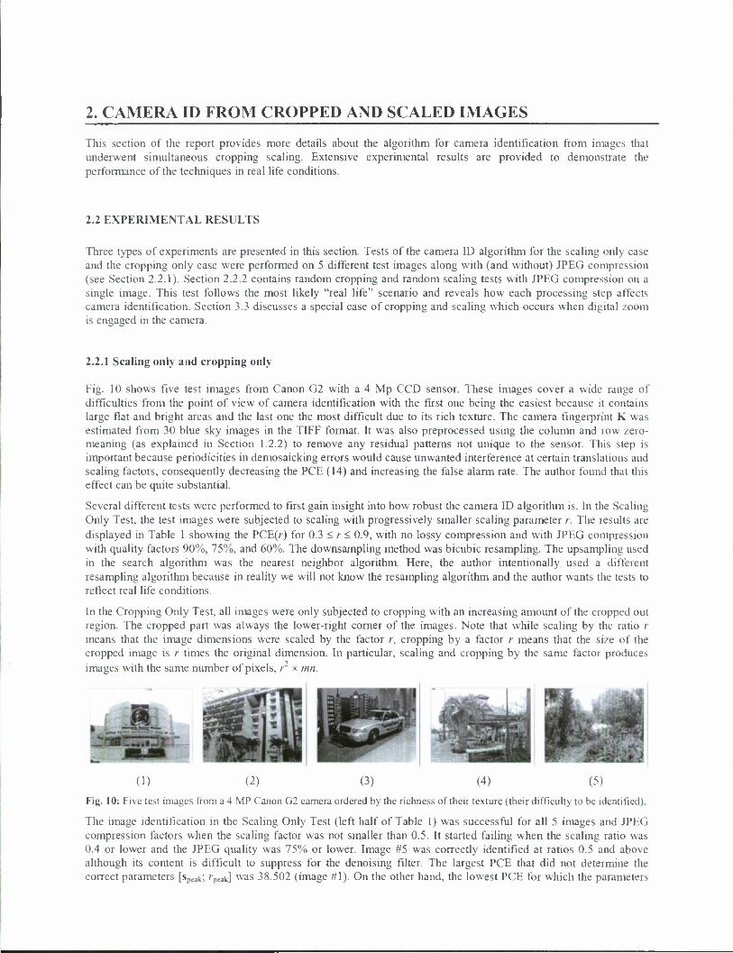
Fig. 10 shows five test images from Canon G2 with a 4 Mp CCD sensor. These images cover a wide range of difficulties from the point of view of camera identification with the first one being the easiest because it contains large flat and bright areas and the last one the most difficult due to its rich texture. The camera fingerprint K was estimated from 30 blue sky images in the TIFF format. It was also preprocessed using the column and row zero- meaning (as explained in Section 1.2.2) to remove any residual patterns not unique to the sensor. This step is important because periodicities in demosaicking errors would cause unwanted interference at certain translations and scaling factors, consequently decreasing the PCE (14) and increasing the false alarm rate. The author found that this effect can be quite substantial.
Several different tests were performed to first gain insight into how robust the camera ID algorithm is. In the Scaling Only Test, the test images were subjected to scaling with progressively smaller scaling parameter r. The results are displayed in Table 1 showing the PCE(r) for 0.3 < r < 0.9, with no lossy compression and with JPEG compression with quality factors 90%, 75%, and 60%. The downsampling method was bicubic resampling. The upsampling used in the search algorithm was the nearest neighbor algorithm. Here, the author intentionally used a different resampling algorithm because in reality we will not know the resampling algorithm and the author wants the tests to reflect real life conditions.
In the Cropping Only Test, all images were only subjected to cropping with an increasing amount of the cropped out region. The cropped part was always the lower-right corner of the images. Note that while scaling by the ratio r means that the image dimensions were scaled by the factor r, cropping by a factor r means that the size of the cropped image is r times the original dimension. In particular, scaling and cropping by the same factor produces images with the same number of pixels, r x mn.
(1) (2) (3) (4) (5)
Fig. 10: Five test images from a 4 MP Canon G2 camera ordered by the richness of their texture (their difficulty to be identified).
The image identification in the Scaling Only Test (left half of Table 1) was successful for all 5 images and JPEG compression factors when the scaling factor was not smaller than 0.5. It started failing when the scaling ratio was 0.4 or lower and the JPEG quality was 75% or lower. Image #5 was correctly identified at ratios 0.5 and above although its content is difficult to suppress for the denoising filter. The largest PCE that did not determine the correct parameters [speak; /"peak] was 38.502 (image #1). On the other hand, the lowest PCE for which the parameters

were correctly determined was 35.463 (also for image #1). In some cases, the maximum value of NCC did occur for the correct cropping and scaling parameters but the identification algorithm failed because the PCE was below the threshold set to achieve PFA < 10~5.
Image cropping has a much smaller effect on image identification (the Cropping Only Test part of Table 1). It was possible to correctly determine the exact position of the cropped image within the (unknown) original in all tested cases. The PCE was consistently above 130 even when the images were cropped to the small size 0.3m x 0.3/J and compressed with JPEG quality factor 60.
Scaling Only Test Cropping Only Test
Im. #1 Im. #2 Im. #3 Im. #4 Im. #5 Im. #1 Im. #2 Im. #3 Im. #4 Im. #5
TIFF 68003 32325 28570 20092 2964 14624 9157 7789 8961 3106 r = 0.9 Q90 28951 12834 11347 6971 1515 20905 11475 8223 7348 2637 r=45.1 Q75 6131 3343 3436 2225 793 7192 4509 4668 3193 1480
Q60 1778 1245 1291 1037 461 2751 2029 2227 1706 919 TIFF 72971 35086 30128 17494 2260 9282 8148 7764 8043 3058
r = 0.8 Q90 19041 8045 7080 4171 955 15287 8988 8251 6060 2329
r=48.3 Q75 2980 1610 1736 1115 417 5698 2979 3977 2550 1226
Q60 763 645 614 348 222 2216 1224 1916 1337 754 TIFF 41835 20058 17549 9674 910 6496 7986 7384 6030 250S
/- = 0.7 Q90 8255 3642 3731 1938 410 11434 7887 9210 4533 2037 r=50.4 Q75 1316 724 979 507 170 4565 2593 3807 2142 995
Q60 328 318 406 203 124 1774 1155 1860 1139 622 TIFF 42192 18991 16902 8986 1001 4896 8249 6550 4353 1971
/=0.6 Q90 4619 2060 2195 1311 422 7679 6328 8574 2918 1445 r=52.1 Q75 625 399 476 214 117 2883 1951 3443 1255 682
Q60 190 166 196 85 53 1166 709 1568 669 459 TIFF 24767 10719 9442 4781 487 4339 6592 5216 3006 1599
r = 0.5 Q90 1721 997 927 533 196 6314 3989 6996 2206 1265 r=53.5 Q75 211 168 221 134 111 2622 1089 2799 1003 695
Q60 144 56 70 (50) 58 1216 398 1322 574 464 TIFF 8083 3193 2897 1310 123 4008 4469 4163 1881 1086
/• = 0.4 Q90 457 227 280 151 (52) 3730 2274 5178 1230 846 r=54.8 Q75 72 (52) 72 (53) 31 1407 723 2113 570 453
Q60 (35) (43) (43) 26 34 599 255 1006 311 324 TIFF 777 352 477 124 27 3518 1585 3030 916 837
;=0.3 Q90 (46) (41) 60 38 30 2577 742 3414 657 609 r=55.9 Q75 39 32 35 31 35 969 269 1378 300 259
Q60 35 33 35 32 35 461 139 721 164 177
Table 1: PCE in the Scaling Only Test followed by JPEG compression. The PCE is in italic when the scaling ratio was not determined correctly. Values in parentheses are below the detection threshold r (see the leftmost column) for PFA < 10 .
2.2.2 Random cropping and random scaling simultaneously
This series of tests focused on the performance of the search method on image #2. The image underwent 50 simultaneous random cropping and scaling with both scaling and cropping ratios between 0.5 and 1 followed by JPEG compression with the same quality factors as in the previous tests. The maximum PCE values found in each search were sorted by the scaling ratio (since it has by far the biggest influence on the algorithm performance) and plotted the PCE in Fig. 11. The threshold r= 56.315 displayed in the figure corresponds to the worst scenario (largest search space) of 0.5 scaling and 0.5 cropping for false alarm rate below 10~5. In the test, no missed detection occurred for the JPEG quality factor 90, 1 missed detection for JPEG quality factor 75 and scaling ratio close to 0.5, and 5 missed detections for JPEG quality factor 60 when the scaling ratios were below 0.555. Even though these

numbers will vary significantly with the image content, they provide insight into the robustness of the method on real images.
The last test was a large scale test intended to evaluate the real-life performance of the proposed methodology. The database of 720 images contained snapshots spanning the period of four years. All images were taken at the full CCD resolution and with a high JPEG quality setting. Each image was first subjected to a randomly-generated cropping up to 50% in each dimension. The cropping position was also chosen randomly with uniform distribution within the image. The cropped part was further resampled by a scaling ratio re[0.5, 1]. Finally, the image was compressed with 85% quality JPEG. The false alarm was set again to 10~5. Running our algorithm with /,„„, = 0.5 on all images processed this way, we encountered 2 missed detections (Fig. 5a), which occurred for more difficult (textured) images. In all successful detections, the cropping and scaling parameters were detected with accuracy better than 2 pixels in either dimension.
To complement this test, 915 images from more than 100 different cameras were downloaded from the Internet in native resolution, cropped to the 4 Mp size of Canon G2 and subjected to the same random cropping, scaling, and JPEG compression as the 720 images before. No single false detection was encountered. All maximum values of PCE were below the threshold with the overall maximum at 42.5.
2.2.3 Digital zoom
While optical zoom does not desynchronize PRNU with the image noise residual (it is equivalent to a change of scene), when a camera engages digital zoom, it introduces the following geometrical transformation: the middle part of the image is cropped and up-sampled to the resolution determined by the camera settings. This is a special case of our cropping and scaling scenario. Since the cropping may be a few pixels off the center, one needs to search for the scaling factor /• as well as the shift vector s. The maximum digital zoom determines the upper bound on the search for the scaling factor (see Section 1.3.1). For simplicity, the same search is applied for cropping as before although it would be possible to use a restricted search range around the image center. Some cameras allow almost continuous digital zoom (e.g., Fuji E550) while other offer only several fixed values. This is the case of Canon S2. The camera display indicates zoom values "24*", "30*", "37x", and "48*", which correspond to digital zoom scaling ratios 1/2, 1/2.5, 1/3.0833, and 1/4, considering the 12x camera optical zoom. The test using camera fingerprint revealed exact scaling ratios 1/2.025, 1/2.5313, 1/3.1154, and 1/4, corresponding to cropped sizes 1280*960, 1024*768, 832*624, and 648*486, respectively. Thus, in general for camera identification, one may wish to check these digital zoom scaling values first before proceeding with the rest of the search if no match is found. Note that none of the camera manuals for the two tested cameras (Fuji and Canon) contained any information about the digital zoom. The details about their digital zooms were found using the PRNU! Thus, this is an interesting example of using the PRNU as a template to recover processing history or reverse-engineer in-camera processing.
Table 2 shows the maximal PCE on 10 images taken with Canon S2 and Fuji E550, some of which were taken with digital zoom. Both cameras were identified with very high confidence in all 10 cases. Images from Fuji camera yielded smaller maximum PCEs, which suggests that (if the image content is dark or heavily textured) the identification of Fuji E550 camera could be more difficult than Canon S2. The detected cropped dimensions (see Table 2) are either precise or off only by a few pixels. This camera apparently has a much finer increment when adjusting the digital zoom than Canon S2. Since the Fuji E550 user is not informed about the fact that the digital zoom has been engaged, it may be quite tedious to find all possible scaling values in this case. The largest digital zoom the camera offers for full resolution output size is 1.4. Fig. 12 shows images with detected cropped frame for the last two Fuji camera images of the same scene.
The fact that it is possible to obtain previous dimensions of the up-sampled images is an example of "reverse engineering" for revealing image processing history. Such information is potentially useful in forensics sciences even if the source camera is positively known beforehand.

10' 10
10*
U 10 Q-
• I •<
10"
10. 0.5 0.6 0.7 0.8 0.9
scaling factor
(a) JPEG quality factor 90
10
o 10" Q_
10'
10. 0.5 0.6 0.7 0.8 0.9
scaling factor
(b) JPEG quality factor 75
0.5 0.6 0.7 0.8 0.9 1 scaling factor
(c) JPEG quality factor 60
Fig. 11. PCE for image #2 after a series of random scaling and cropping followed by 90% quality JPEG compression.
Canon S2 Fuji E550
Image scaling max cropped scaling max cropped # detected PCE dim detected I'd-: dim
1 3.1154 1351 832x624 1.1530 358 2470x1853 2 2.5313 6020 1024x768 1.3434 238 2120x1590 3 2.0250 2792 1280x960 1.3940 102 2043x1532 4 2.0203 9250 1283x962 1.1837 310 2406x1805 5 2.5313 5929 1024x768 1.0234 576 2783x2087 6 3.1154 3509 832x624 1.0007 328 2846x2135 7 4.0062 2450 647x485 1.0000 314 2848x2136 8 4.0062 1265 647x485 1.0845 1022 2626x1970 9 4.0062 1620 649x487 1.1530 976 2470x1853 10 4.0062 1612 647x485 1.3428 378 2121x1591
Table 2: Detection of scaling and cropping for digitally zoomed images.

Fig. 12: Cropping detected for Fuji E550 images #9 and #10.
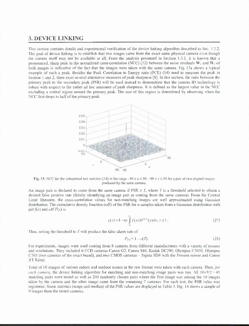
3. DEVICE LINKING
This section contains details and experimental verification of the device linking algorithm described in Sec. 1.3.2. The goal of device linking is to establish that two images came from the exact same physical camera even though the camera itself may not be available at all. From the analysis presented in Section 1.3.1, it is known that a pronounced, sharp peak in the normalized cross-correlation (NCC) (12) between the noise residuals W, and \V2 of both images is indicative of the fact that the images were taken with the same camera. Fig. 13a shows a typical example of such a peak. Besides the Peak Correlation to Energy ratio (PCE) (14) used to measure the peak in Section 1 and 2, there exist several alternative measures of peak sharpness [8]. In this section, the ratio between the primary peak to the secondary peak (PSR) will be used instead to demonstrate that the camera ID technology is robust with respect to the rather ad hoc measures of peak sharpness. It is defined as the largest value in the NCC excluding a central region around the primary peak. The size of this region is determined by observing when the NCC first drops to half of the primary peak.
-50 -50
Fig. 13: NCC for the suboptimal test statistics (14) in the range -50 < u < 50,-50 < v < 50 for a pair of two aligned images produced by the same camera.
An image pair is declared to come from the same camera if PSR > T, where T is a threshold selected to obtain a desired false positive rate (falsely identifying an image pair as coming from the same camera). From the Central Limit Theorem, the cross-correlation values for non-matching images are well approximated using Gaussian distribution. The cumulative density function (cdf) of the PSR for n samples taken from a Gaussian distribution with pdf/(.v) and cdf F(x) is
c(z) = \-nz jf(xz)F"-,(x)dx, z>\ (27)
Thus, setting the threshold to T will produce the false alarm rate of
PFA=\-c(T). (28)
For experiments, images were used coming from 8 cameras from different manufacturers with a variety of sensors and resolutions. They included 6 CCD cameras Canon G2, Canon S40, Kodak DC290, Olympus C3030, Olympus C765 (two cameras of the exact brand), and two CMOS cameras - Sigma SD9 with the Foveon sensor and Canon XT Rebel.
Total of 10 images of various indoor and outdoor scenes in the raw format were taken with each camera. Then, for each camera, the device linking algorithm for matching and non-matching image pairs was run. All 10x9/2 =45 matching pairs were tested as well as 200 randomly chosen pairs where the first image was among the 10 images taken by the camera and the other image came from the remaining 7 cameras. For each test, the PSR value was registered. Some statistics (range and median) of the PSR values are displayed in Table 3. Fig. 14 shows a sample of 9 images from the tested cameras.

To see how the reliability of the device linking algorithm deteriorates with lossy compression, the same experiment was repeated after all images were compressed using JPEG with quality factor 90 and 75. The results are also shown in Table 3.
Regardless of the quality factor, the largest value of the PSR for an unmatched pair (among 3x8x200 pairs) was 1.3, while the smallest value for a matched pair (out of 3x8x45 pairs) was 1.0. Setting T= 1.4 would in this test produce zero false alarms (incorrectly classified non-matching pair) with the probability of false alarm PFA s 5x10 . Table 3 shows the percentage of correctly classified matching pairs with this theoretical false alarm rate. For example, 41 correctly classified cases out of 45 pairs of the raw Canon Rebel images result in 91.1% probability of correct detection of a matched pair (PDM).
The PDM is usually very high for raw images but deteriorates with a decreasing JPEG quality factor. Since the PRNU term IK is multiplicative, very dark images are more likely to be misclassified. The same is also true for highly textured images due to the limitation of the denoising filter, which fails to filter out the image content.
Matched Pairs Unmatched Pairs PDM
Matched Pairs Unmatched Pairs PDM
min 1 med max min med max min med max min med max
Canon G2
Raw 7.4 11.6 24.3 1.00 1.03 1.19 100",, Olympus C765-1
Raw 3.6 5.5 9.1 1.00 1.04 1.28 100%
Q90 4.1 6.6 16.5 1.00 1.03 1.20 100% Q90 1.8 3.6 4.8 1.00 1.03 1.25 100%
Q75 1.2 2.6 6.3 1.00 1.03 1.28 97.8% Q75 1.2 1.8 2.9 1.00 1.03 1.26 88.9%
Raw 8.8 12.6 23.2 1.00 1.03 1.30 100% Olympus C765-2
Raw 1.9 3.0 8.3 1.00 1.03 1.29 100% Canon
S40 Q90 5.3 S.4 14.3 1.00 1.03 1.30 100",, Q90 1.1 1.9 4.6 1.00 1.03 1.24 86.7%
Q75 2.2 3.3 5.2 LOO 1.03 1.30 100% Q75 1.0 1.2 2.7 1.00 1.04 1.26 33.3% Raw 1.0 2.9 5.7 1.00 1.03 1.21 91.1",,
Olympus C3030
SHQ 8.4 15.0 28.1 1.00 1.04 1.26 100% Canon XT
Rebel Q90 1.0 1.7 2.6 1.00 1.03 1.30 57.8% 090 4.7 8.0 15.1 1.00 1.04 1.25 100%
Q75 1.0 1.1 1.6 1.00 1.04 1.27 4.4% Q75 1.9 3.7 6.9 1.00 1.03 1.26 100%
Kodak DC290
Raw 2.2 7.2 13.8 1.00 1.03 1.19 100% Sigma SD9
Raw 3.8 8.0 14.1 1.00 1.03 1.23 100%
Q90 1.1 2.7 5.4 1.00 1.04 1.24 93.3% Q90
Q75
1.4 3.2 6.9 1.00 1.03 1.25 95.6%
Q75 1.0 1.4 2.2 1.00 1.03 1.23 48.9% 1.0 1.5 3.7 1.00 1.04 | 1.24 55.6%
Table 3: Minimum, median, and maximum PSR and probability of detection (PDM) for tested image pairs from all cameras. The decision threshold was set so that the probability of false alarms was PF/t = 5x 10" .
Fig. 14: Some sample images used in our tests
4. VIDEO IDENTIFICATION
This section contains extensive experimental verification of the fingerprint linking algorithm proposed for identification of video clips in Section 1.3.3. This algorithm is used to decide whether two video-clips A and B were produced by the exact same camcorder. Let KA and KB be the PRNUs estimated from both clips. Because the PRNU is a unique signature of the camera, the task of origin identification is equivalent to The test statistic (12) is the NCC between the estimates of both fingerprints, kA and KB.
4.1 REMOVING ARTIFACTS FROM THE FINGERPRINT
Because PRNUs from two different sensors are uncorrelated, if both clips are indeed from the same camcorder, one expects to see a sharp peak in the NCC and a correspondingly large PCE. However, almost all camcorders use DPCM-Block DCT transform-type video coding, such as MPEG-x and H.26x. This creates (i) ringing artifacts at the frame boundaries caused by the padding required for frame dimensions not divisible by the block size and by operations such as motion estimation/compensation for out of frame movement; (ii) 16x16 blockiness artifacts inside the frame because most standard codecs are based on 16x16 macroblocks. These periodic pulse-like signals (Fig. 15a) propagate through the denoising filter into the estimated fingerprints and cause false correlations between otherwise uncorrelated fingerprints. Thus, they must be removed before calculating the NCC. Because of the heavy compression typically encountered in video coding, the fingerprints need to be estimated from thousands of video-frames and the periodic artifacts accumulate more than in the case of camera identification from images.
The boundary artifacts can be easily removed by cropping ~8 pixel wide boundaries in the spatial domain. The periodic pulse-like blockiness artifacts can be removed in the Fourier domain (Fig. 15b) by attenuating the Fourier coefficients at frequencies where most of the artifacts' energy is located. To illustrate how to locate the frequencies of these periodic pulse-like signals, consider the following one-dimensional periodic signal x{n) = 8{n -16m), 0 < n < N -1 whose DFT transform is X(r)
. ( 2rr k ) sin r
\X{r)\= \Nn6\K (29) sin
V/V/162
where k = L(A'-l)/16j and /' is the DFT index. Equation (29) shows that the energy of \X(r)\ concentrates around frequencies of integer multiples of Ml6. Therefore, setting X(r) = 0 for those frequencies and their neighborhood (3-6 times frequency resolution) effectively reduces the strength of the periodic signal. In the experiments described in this section, a similar effect idea was realized using an FFT domain filter designed to mitigate the deteriorating effect of blockiness on the NCC. Fig. 15b and c show the Fourier magnitude of the fingerprint and the filtered fingerprint. Since in practice the NCC is calculated in the Fourier domain, one can conveniently perform blockiness removal at the same time. Furthermore, other artifacts that manifest themselves as peaks in the Fourier domain will be suppressed, such as artifacts due to color filter array interpolation and other hardware or software operations already mentioned in Section 1.2.

33
(a) (b) (c)
Fig. 15: (a) Blockiness artifacts in a small magnified portion of the estimated fingerprint; (b) Fourier magnitude of (a); (c) Fourier magnitude after removing the artifacts in the DFT domain.
4.2 EXPERIMENTAL RESULTS
This section contains selected experiments illustrating the effectiveness of the proposed forensic method for identifying the origin of video clips. Twenty-five consumer digital camcorders were used (20 SONY, 4 Hitachi, 1 Canon). The recording media was Mini-DV or DVD-RW and the sensor resolution varied from 0.68MP^.l MP. Three camcorders (one Canon DC40 and two camcorders of the same model SONY DCR- DVD105) were selected and tested against the remaining clips. The two SONY camcorders will be addressed as SONY DCR-1 and SONY DCR-2. With each camcorder, several high quality video clips were prepared (roughly 6 Mb/sec, DVD quality, resolution 536x720, frame rate 30 Hz, MPEG-2 VOB format) of various indoor and outdoor scenes. The clips contained brief periods of optical zooming in/out and panning. Some of the videos contained quickly moving objects (e.g., cars) while others had panned static scenes. All the camcorders had their Electronic Image Stabilization (EIS) and digital zooming turned off. All scenes were taped with the fully automatic settings.
The videos were also transcoded to low-bit rate formats, such as the MPEG-4 XviD format (~1 Mbit/sec), the RealPlay format (-750 Kbit/sec), and the MPEG-4 DivX format (-450 Kbit/sec). These formats represent the most popular choices for distribution of video over the Internet today.
4.2.1 VOB, XviD, RealPlay, DivX vs. VOB
This purpose of this test is to investigate whether it is possible to correctly identify the source camera from videos that were transcoded to 4 different formats and bit-rates. First, the fingerprints were estimated from a 40-second randomly selected video segment from SONY DCR-1 clips in the VOB format. Then, three more fingerprints were estimated from three transcoded formats, Xvid, RealPlay, and DivX, obtaining thus four SONY DCR-1 fingerprints of varying quality. Then, the NCCs were computed with the fingerprints from a different 40-second SONY DCR-1 video clip in the VOB format and 24 fingerprints from 24 40-second video clips from all the other camcorders, also in the VOB format. For the SONY DCR-1, SONY DCR-2, and Canon DC40 camcorders, Fig. 16 shows the NCC surface and the PCE in a pictorial form. The results for the remaining 22 camcorders are summarized in the table below the figure.
In the same manner, two 40-second randomly selected SONY DCR-2 clips and Canon DC40 clips were randomly chosen and tested against all the fingerprints from the 25 camcorders (obtained from VOBs). The results are shown in the same format in Fig. 16b and Fig. 16c. The figures reveal the reliability of the proposed identification approach for all four bit rates. Also, one can see that with the same number of frames, the quality of the estimated fingerprints decreases as the video quality decreases (measured by the bit rate).

34
The degradation of the estimated fingerprints is the reason for deterioration of the NCC surface (and the decrease in PCE and correlation coefficient). Regardless of the video format, the PCE and the correlation coefficients obtained for the matched case are by several orders of magnitude larger than for the unmatched case.
4.2.2 Xvid vs. Xvid for clips of different length
In the second experiment, two fingerprints were estimated from two 40-second SONY DCR-2 video clips of different scenes in the XviD-format and the NCC between them was calculated. Then, the same process was repeated with length of the clips increased to 80 seconds and 120 seconds. The resulting NCCs are shown in Fig. 17.
4.2.3 Low bit-rate experiment
The third experiment focused on identification of "Internet-quality" clips with low resolution and very low bit-rate. Two clips were used - the one from SONY DCR-1 and one from Canon DC40 taken at LP resolution of 264x352 pixels. Both clips were then transcoded to 150kb/sec. in the RMVB format. Then both clips were tested for the presence of a fingerprint estimated from four 2.5min VOB clips from SONY DCR-1. The NCC surfaces and PCEs are shown in Figure 18. The identification is again possible and improves with the length of the clip.
SONY DCR-1 40 Sees, SONY DCR-2 40 Sees, Canon DV40 40 Sees, 6Mb/s, VOB 6Mb/s, VOB 6Mb/s, VOB
SONY ] ' •i
!
DCR-1 ** .:
40 Sees M
6Mb/s VOB
»** .no
~"~M wt
«' .-*•.' " tt >- **" t •* *
IN HI-
1W
MO Mfl
(a) PCE = 9.0e+04, 0.6318
CorrCocf = (b) PCE = 41.1, CorrCoef =0.0016 (c) PCE = 34.1. CorrCoef = 0.0028
SONY i.is
u 0^
DCR-1 MS
•' "
40 Sees » , •
IMb/s XviD • *•-.
»"' ••..-••••"'«
(d) PCE = 6.2e+03. 0.1512
•
CorrCoef = (e)
» ' - „ --- " M
PCE = 37.5, CorrCoef = -0.0023
MS m
to PCE = 41.2, CorrCoef =0.0024

35
SONY U. ... .«
DCR-1 U, i^^&i r* •••<'. j t .-"f r -4., ; '"<
Ijf • '
40 Sees ' iflii^ . .... • . '
750 Kb/s RealPlay
Ml *J2
1'" IM
M
MO HW
(g) PCE = 936.8, CorrCoef = 0.0573 (h) PCE = 35.3, CorrCoef = -0.0022 (i) PCE = 27.6, CorrCoef - 0.0025
SONY
... •it.
wL-J""'"' IM .
DCR-1
40 Sees
DM • •
v . •?:•:'/'::' •' *' - ';v.:'"'.,•."•>••,:., tMt
M4.
*
450 Kb/s DivX
m
(j) PCE = ].2e+03, CorrCoef = 0.0657
(k) PCE = 56.7.1, CorrCoef = 0.0024
(1) PCE - 35.8, CorrCoef = -O.00O8
Other 22 SONY DCR-1 SONY DCR-1 SONY DCR-1 SONY DCR-1 camcorders
40 Sees, 6Mb/s 40 Sees, 1 Mb/s 40 Sees, 750 Kb/s 40 Sees, 450 Kb/s VOB XviD RP DivX
CorrCoef PCE CorrCoef PCE CorrCoef PCE CorrCoef PCE
Min -0.0041 28.0 -0.0044 28.2 -0.0053 26.8 -0.0035 25.5
Max 0.0084 89.0 0.0045 90.3 0.0046 73.9 0.0050 156.9 Statistics
-0.0004 43.2 0.0005 37.3 0.0012 32.5 0.0007 38.7 Median
Fig. 16a: NCC of PRNUs of 4 differently transcoded versions of a SONY DCR-1 clip with PRNUs estimated from 25 camcorders in the VOB format.

36
SONY DCR-1 Sees, 6Mb/s, VOB
40 SONY DCR-2 Sees, 6Mb/s, VOB
40 Canon DV40 Sees, 6Mb/s, VOB
40
SONY DCR-2
40 Sees 6Mb/s VOB
(a) PCE = 38.0, CorrCoef 0.0028
(b) PCE = 8.2e+04. CorrCoef =0.6464
(c) PCE = 38.8, CorrCoef 0.0058
SONY DCR-2
40 Sees
IMb/s XviD
(d) PCE = 32.8, CorrCoef 0.0006
(e) PCE = 1.0e+04, CorrCoef =0.2038
(f) PCE = 34.8, CorrCoef 0.0006
SONY DCR-2
40 Sees
750 Kb/s RealPla y
(g) PCE = 28.1, CorrCoef 0.0005
(h) PCE = 2.1e+03, CorrCoef = 0.0867
(i) PCE = 28.0, CorrCoef 0.0013
SONY DCR-2
40 Sees
450 Kb/s DivX (j) PCE = 37.2, CorrCoef
-0.0016 (k) PCE = 1.9e+03, CorrCoef =0.0871
(1) PCE = 33.6, CorrCoef -0.0018

37
Other 22 camcorders
SONY DCR-2
40 Sees, 6Mb/s VOB
SONY DCR-2
40 Sees, IMb/s XviD
SONY DCR-2
40 Sees, 750 Kb/s RP
SONY DCR-2
40 Sees, 450 Kb/s, DivX
CorrCoef PCE CorrCoef PCE CorrCoef PCE CorrCoef PCE
Statistics
Min -0.0070 22.6 -0.0058 29.5 -0.0060 28.4 -0.0044 27.6
Max 0.0059 73.7 0.0051 100.8 0.0059 116.5 0.0065 61.6
Median -0.0022 43.1 -0.0015 38.5 -0.0005 39.3 0.0005 35.8
Fig. 16b: NCC of PRNUs of 4 differently transcoded versions of a SONY DCR-2 clip with PRNUs estimated from 25 camcorders in the VOB format.
SONY DCR-1 40 SONY DCR-2 40 Canon DV40 40 Sees, 6Mb/s, VOB Sees, 6Mb/s, VOB Sees, 6Mb/s, VOB
Canon
... ... • -i.
DV40 •
*),
40 Sees 02 • •7, ' ^^^B ^BflMWP^ 6Mb/s ;••--, _.-••- '•'
VOB - „. • w '..-•' •*
(a) PCE = 38.2, CorrCoef = 0.0032
(b) PCE = 38.7, CorrCoef = 0.0072
(c) PCE = 3.7e+04, CorrCoef = 0.4644
Canon e.i. •
(.IS
\ ..„
DV40
40 Sees
IMb/s •sJ
M . 1*»
-•-••"" •
M MS,
„>~. • ...— .
XviD (d) PCE = 35.1, CorrCoef = (e) PCE = 55.0, CorrCoef = (f) PCE = 2.0e+03, -0.0002 0.0002 CorrCoef =0.0982
Canon DV40 .«. M*. .. 40 Sees ... *.<M- j Ml
750 Kb/s RealPla *m
a»2
' Ml
1
"^i;:. ' . ',, sit****
y M' "«
m m .'.'",„ *

38
(g) PCE = 25.8, CorrCoef = (h) PCE = 31.3, CorrCoef = (i) PCE = 370.9, CorrCoef = -0.0034 -0.0016 0.0404
Canon DV40
Ml
Ml
j MX
nee
IJM
••J
•Ml,
: '
40 Sees . . . - '- • • , : • ;
450 $»? . .. z
M"^'-.^ .•-'"". .-• """ "»
•1)
* Kb/s »' "V '
to;" ittt »"> <•'•
DivX (j) PCE = 32.6, CorrCoef = (k) PCE = 40.5, CorrCoef = (1) PCE = 390.0, CorrCoef = 0.0022 -0.0008 0.0429
Other 22
camcorders
Canon DV40 40 Sees, 6Mb/s VOB
Canon DV40 40 Sees, IMb/s XviD
Canon DV40
40 Sees, 750 Kb/s RP
Canon DV40
40 Sees, 450 Kb/s DivX
CorrCoef PCE CorrCoef PCE CorrCoef PCE CorrCoef PCE
Statistic s
Min -0.0058 26.8 -0.0033 28.7 -0.0045 32.5 -0.0041 26.0
Max 0.0111 121.1 0.0080 122.3 0.0050 94.5 0.0039 82.2
Median 0.0021 56 -0.0012 38.4 -0.0013 32.4 -0.0005 39.9
Fig. 16c: NCC of PRNUs of 4 differently transcoded versions of a Canon clip with PRNUs estimated from 25 camcorders in the VOB format.

SONY DCR-2, 40 Sees, IMb/s, XviD NCC
SONY DCR-2, 40 Sees, IMb/s, XviD
SONY DCR-2, 80 Sees, IMb/s, XviD NCC
SONY DCR-2, 80 Sees, IMb/s, XviD
39
SONY DCR-2, 120 Sees, IMb/s, XviD NCC
SONY DCR-2, 120 Sees, IMb/s, XviD
(a) PCE = 9.0e+03, CorrCoef 0.1893
(b) PCE = 1.8e+04, CorrCoef 0.2830 (c) PCE = 2.8e+04, CorrCoef
0.3630
Fig. 17: NCCs of PRNUs from different SONY DCR-2 XviD-format video clips with the length 40, 80, and 120 seconds.
SONY DCR-1 10 Canon DC40 10 SONY DCR-1 40 Mins, 150Kb/sRMVB Mins, 150 Kb/s RMVB Mins, 150 Kb/s RMVB
SONY DCT- ' ' 1 10 l [U. ' o«2
._••- •'•
>. ooa. 006.
Mins 1.5
m;. oo<
•j-
oei • •
'•' 00*.
0 02.
0. ''
Mb/s
VOB tin,
•
003. 5) t^
oo: 0 04.
so' 50
SO 40 SO 40
(a) PCE = 111, CorrCoef = (b) PCE = 22, CorrCoef = (c) PCE = 196, CorrCoef = 0.0580 0.0018 0.0834
Fig. 18: NCC surface and PCE coefficient for two low-resolution, low bit-rate clips from SONY DCR-1 and Canon DC40 with PRNU estimated from a 10 minute VOB clip from SONY DCR-1. 4a) is for a 10 minute clip from SONY DCR-1 and 4b) for 40 minute clip.

REFERENCES [1] Janesick, J.R.: Scientific Charge-Coupled Devices, SPIE PRESS Monograph vol. PM83, SPIE-The
International Society for Optical Engineering, January, 2001.
[2] Healey, G. and Kondepudy, R.: "Radiometric CCD Camera Calibration and Noise Estimation." IEEE Transactions on Pattern Analysis and Machine Intelligence, vol. 16(3), pp. 267-276, March, 1994.
[3] Kay, S.M.: Fundamentals of Statistical Signal Processing, Volume I, Estimation theory, Prentice Hall, 1998.
[4] Kay, S.M.: Fundamentals of Statistical Signal Processing, Volume II. Detection theory. Prentice Hall, 1998.
[5] El Gamal, A„ Fowler, B. Min, H., and Liu, X.: "Modeling and Estimation of FPN Components in CMOS Image Sensors." Proc. SPIE, Solid State Sensor Arrays: Development and Applications II, vol. 3301-20, San Jose, CA, pp. 168-177, January 1998.
[6] Filler, T., Fridrich, J., and Goljan, M.: "Using Sensor Pattern Noise for Camera Model Identification." To appear in Proc. IEEE ICIP 08, San Diego, CA, September 2008.
[7] Holt, C.R.: "Two-Channel Detectors for Arbitrary Linear Channel Distortion," IEEE Trans, on Acoustics. Speech, andSig. Proc, vol. ASSP-35(3), pp. 267-273, March 1987.
[8] Vijaya Kuma, B.V.K. and Hassebrook, L.: "Performance Measures for Correlation Filters," Appl. Opt. 29,2997-3006, 1990.
[9] Goljan, M. and Fridrich, J.: "Camera Identification from Cropped and Scaled Images." Proc. SPIE Electronic Imaging, Forensics, Security, Steganography, and Watermarking of Multimedia Contents X, vol. 6819, San Jose, California, January 28 - 30, pp. 0E-1-0E-13 2008.
[10]Goljan, M. and Fridrich, J.: "Camera Identification from Printed Images." Proc. SPIE Electronic Imaging, Forensics, Security, Steganography, and Watermarking of Multimedia Contents X, vol. 6819, San Jose, California, January 28 - 30, pp. OI-1-OI-12, 2008.
[1 lJGoljan, M., Mo Chen, and Fridrich, J.: "Identifying Common Source Digital Camera from Image Pairs." Proc. IEEE ICIP 07, San Antonio, TX, 2007.
[12]Chen, M.. Fridrich, J., and Goljan, M.: "Source Digital Camcorder Identification Using CCD Photo Response Non-uniformity." Proc. SPIE Electronic Imaging, Security. Steganography. and Watermarking of Multimedia Contents IX, vol. 6505, San Jose, California, January 28 - February 1, pp. 1G-1H, 2007.
[13] Chen, M., Fridrich, J., Goljan, M., and Lukas, J.: "Determining Image Origin and Integrity Using Sensor Noise." IEEE Transactions on Information Security and Forensics, vol. 3(1), pp. 74-90, March 2008.
[14]Gou, H., Swaminathan, A., and Wu, M.: "Robust Scanner Identification Based on Noise Features." Proc. SPIE, Electronic Imaging, Security, Steganography, and Watermarking of Multimedia Contents IX, vol. 6505, January 29-February 1, San Jose, CA, pp. 0S-0T, 2007.
[15]Khanna, N., Mikkilineni, A.K., Chiu, G.T.C., Allebach, J.P., and Delp, E.J. Ill: "Forensic Classification of Imaging Sensor Types." Proc. SPIE, Electronic Imaging, Security. Steganography. and Watermarking of Multimedia Contents IX, vol. 6505, January 29-February 1, San Jose, CA, pp. 0U-0V, 2007.

42
[16]Sankur, B., Celiktutan, O., and Avcibas, I.: "Blind Identification of Cell Phone Cameras." Proc. SPIE, Electronic Imaging, Security, Steganography, and Watermarking of Multimedia Contents IX, vol. 6505, January 29-February 1, San Jose, CA, pp. 1H—II, 2007.
[17]Gloe, T., Franz, E., and Winkler, A.: "Forensics for Flatbed Scanners." Proc. SPIE, Electronic Imaging, Security, Steganography, and Watermarking of Multimedia Contents IX, vol. 6505, January 29-February 1, San Jose, CA, pp. II—1J, 2007.
[18]Khanna, N., Mikkilineni, A.K., Chiu, G.T.C., Allebach, J.P., and Delp, E.J. Ill: "Scanner Identification Using Sensor Pattern Noise." Proc. SPIE, Electronic Imaging, Security, Steganography. and Watermarking of Multimedia Contents IX, vol. 6505, January 29-February 1, San Jose, CA, pp. 1K-1L, 2007.
[19]Sutcu, Y., Bayrarn, S., Sencar, H.T., and Memon, N.: "Improvements on Sensor Noise Based Source Camera Identification." Proc. IEEE International Conference on Multimedia and Expo, pp. 24-27, July, 2007.
[20]Bloy, G.J.: "Blind Camera Fingerprinting and Image Clustering." IEEE Transactions on Pattern Analysis and Machine Intelligence, vol. 30(3), pp. 532-534, March 2008.
[21 ] Khanna, N., Chiu, G.T.-C, Allebach, J.P., and Delp, E.J.: "Forensic Techniques for Classifying Scanner, Computer Generated and Digital Camera Images." Proc. IEEE ICASSP, pp. 1653 - 1656, March 31 - April 4, 2008.
[22]Mihcak, M.K., Kozintsev, I., and Ramchandran, K.: "Spatially Adaptive Statistical Modeling of Wavelet Image Coefficients and its Application to Denoising." Proc. IEEE Int. Conf. Acoustics, Speech, and Signal Processing, Phoenix, AZ, vol. 6, pp. 3253-3256, March 1999.
|23]K.harrazi, M., Sencar, H.T., and Memon, N.: "Blind Source Camera Identification", Proc. ICIP' 04, Singapore, October 24-27, 2004.
[24] Bayrarn, S., Sencar, H.T., and Memon, N.: "Source camera identification based on CFA interpolation." ICIP 05, Genoa, Italy, September 2005.
[25]Swaminathan, A., Wu, M., and Liu, K.J.R.: "Non-intrusive Forensic Analysis of Visual Sensors Using Output Images," IEEE Int. Conf. on Acoustics, Speech, and Signal Processing (ICASSP'06), May 2006.
[26] Geradts, Z., Bijhold, J., Kieft, M., Kurosawa, K., Kuroki, K., and Saitoh, N.: "Methods for Identification of Images Acquired with Digital Cameras", Proc. of SPIE, Enabling Technologies for Law Enforcement and Security, vol. 4232, pp. 505-512, February 2001.
[27]Lukas, J. Fridrich, J., and Goljan, M.: "Digital Camera Identification from Sensor Pattern Noise," IEEE Transactions on Information Security and Forensics, vol. 1(2), pp. 205-214, June 2006.
[28] Chen, M., Fridrich, J., and Goljan, M.: "Digital Imaging Sensor Identification (Further Study)," Proc. SPIE Electronic Imaging, Security, Steganography, and Watermarking of Multimedia Contents IX, vol. 6505, San Jose, California, January 28 - February 1, pp. 0P-0Q, 2007.
[29] Cox, I., Miller, M.L., and Bloom, J.A.: Digital Watermarking, Morgan Kaufmann, San Francisco, 2001.
[30] Swaminathan, A., Wu, M., and Liu, K.J.R.: "Image Authentication via Intrinsic Fingerprints." Proc. SPIE, Electronic Imaging, Security, Steganography, and Watermarking of Multimedia Contents IX, vol. 6505, January 29-February 1, San Jose, CA, pp. 1J-1K, 2007.

43
[31 ] Kurosawa, K., Kuroki, K., and Saitoh, N.: "CCD Fingerprint Method - Identification of a Video Camera from Videotaped Images." Proc. ICIP'99, Kobe, Japan, pp. 537-540, October 1999.
[32] Lukas, J., Fridrich, J., and Goljan, M: "Digital Camera Identification from Sensor Pattern Noise." IEEE Transactions on Information Security and Forensics, vol. 1(2), pp. 205-214, June 2006.
[33] Ng, T.-T., Chang, S.-F., and Sun, Q.: "Blind Detection of Photomontage Using Higher Order Statistics." Proc. IEEE International Symposium on Circuits and Systems, vol. 5, Vancouver, Canada, pp. v-688-v- 691,2004.
[34] Avcibas, I., Bayram, S., Memon, N., Ramkumar, M., and Sankur, B.: "A Classifier Design for Detecting Image Manipulations." Proc. ICIP'04, vol. 4, pp. 2645-2648, 2004.
[35] Lin, Z., Wang, R., Tang, X., and Shum, H.-Y.: "Detecting Doctored Images Using Camera Response Normality and Consistency." Proc. IEEE Computer Society Conference on Computer Vision and Pattern Recognition, vol. 1, pp. 1087-1092, 2005.
[36]Popescu, A.C. and Farid, H.: "Exposing Digital Forgeries by Detecting Traces of Resampling." IEEE Transactions on Signal Processing, vol. 53(2), pp. 758-767, 2005.
[37]Popescu, A.C. and Farid, H.: "Exposing Digital Forgeries in Color Filter Array Interpolated Images." IEEE Transactions on Signal Processing, vol. 53(10), pp. 3948-3959, 2005.
[38] Johnson, M.K. and Farid, H.: "Exposing Digital Forgeries by Detecting Inconsistencies in Lighting." Proc. ACM Multimedia and Security Workshop. New York, pp. 1-9, 2005.
[39]Farid, H.: "Exposing Digital Forgeries in Scientific Images." Proc. ACM Multimedia & Security Workshop. Geneva, Switzerland, pp. 29-36, 2006.
[40]Johnson, M.K. and Farid, H.: "Exposing Digital Forgeries Through Chromatic Aberration." Proc. ACM Multimedia and Security Workshop. Geneva, Switzerland, pp. 48-55, 2006.
[41] Chen, W. and Shi, Y.: "Image Splicing Detection Using 2D Phase Congruency and Statistical Moments of Characteristic Function." Proc. SPIE, Electronic Imaging, Security, Steganography, and Watermarking of Multimedia Contents IX, vol. 6505, January 29-February 1, San Jose, CA, pp. 0R-0S, 2007.
[42] Fridrich, J., Soukal, D., and Lukas, J.: "Detection of Copy-Move Forgery in Digital Images." Proc. Digital Forensic Research Workshop. Cleveland, August 2003.
[43]Popescu, A.C. and Farid, H.: "Exposing Digital Forgeries by Detecting Duplicated Image Regions." Technical Report. TR2004-515. Dartmouth College, Computer Science, 2004.
[44] Lukas, J., Fridrich, J., and Goljan, M.: "Detecting Digital Image Forgeries Using Sensor Pattern Noise." Proc. SPIE, Electronic Imaging, Security, Steganography, and Watermarking of Multimedia Contents VIII, vol. 6072. San Jose, California, pp. 0Y1-0Y11, 2006.
[45]Bayram, S., Avcibas, I., Sankur, B. and Memon, N.: "Image Manipulation Detection," Journal of Electronic Imaging, vol. 15(4), 041102, 2006.
[46]Dirik, A., Sencar, E., Husrev T., Memon, N., and Khrazzi, M.: "Source Camera Identification Based on Sensor Dust Characteristics." Proc. IEEE Workshop on Signal Processing Applications for Public Security and Forensics, SAFE '07. April 11-13, 2007, pp. 1-6.