Report on the Central Baltic River GIG Macrophyte Intercalibration Exercise June 2007

ANNEX: NATIONAL MACROPHYTE METHODS FR | DE | PL | BE (WL) | UK | BE (FL)

Monitoring and assessment of the quality element Macrophytes in Rivers FRANCE Status: national norm, defined as the official method for rivers assessment (BQE : Macrophytes) for national monitoring networks (reference network and surveying network).

Original method reference:

Haury J., Peltre M.-C., Trémolières M., Barbe J., Thiébaut G., Bernez I., Daniel H., Chatenet P., Haan-Archipof G., Muller S., Dutartre A., Laplace-Treyture C., Cazaubon A., Lambert-Servien E., 2006. A new method to assess water trophy and organic pollution – the Macrophytes Biological Index for Rivers (IBMR): its application to different types of river and pollution. Hydrobiologia 570:153-158.

National norm reference:

NF T 90-395 (AFNOR, October 2003). Water quality – Determination of the Macrophytes Biological Index for Rivers (IBMR). Which indicators are used? Macrophytes types The macrophytes taken into account for recording are all macrophytic vegetation forms which have at least the stem basis into water in low water conditions. This definition includes 208 taxa, from different floristic groups:

- Emergent phanerogams (helophytic or amphibious forms), - Anchored submerged phanerogams, - Free-floating and floating-leaved phanerogams, - Pteridophytes, - Bryophytes (Mosses and Liverworts), - Macro-algae (Characea), - Filamentous and thallus colonies algae, - Aquatic lichens, - Heterotrophic organisms (filamentous bacteria and fungus).

Taxonomic level The required taxonomic level for determination is:

- Phanerogams: species - Bryophytes: species - Macro-algae (Characea) : species - Colonial algae: genus - Lichens: species - Heterotrophic organisms: genus.

Macrophytes abundance The abundance scale uses 5 logarithmic/algebric classes of abundance, as given in table 1.

Table 1. The macrophytic taxa abundance scale for IBMR.

class % cover description 1 < 0.1 Just present 2 0.1 - 1 Few covering and few frequent 3 1.1 - 10 Fairly covering and fairly frequent 4 11 - 50 Middling covering 5 > 50 Very abundant or covering

Indicative value IBMR is trophic-level oriented by the score assigned at each contributive taxon. These scores are representative of oligotrophy affinity (1: hypereutrophic; 20: very ologotrophic). The index responds also to the habitat structure (bank shape, habitat type, substrate). Complementary habitat description A habitat description is completed with each macrophytes record. The registered parameters are linked to:

- Observation conditions, - Flowing type, - Substrate, - General aquatic vegetation aspect (total cover for each macrophytes floristic /

functional type) How are these indicators monitored? Sampling strategy An exhaustive record is completed on a 100 m. river stretch. The norm is complemented by a technical framework requiring to proceed within 2 different facies (fast as a priority, slow secondarily). Most of phanerogams are identified on field, bryophytes and algae are sampled to determine them in lab. When is monitored and with which frequency? The IBMR surveys must be carried out during the main vegetative period, i.e. 15th June – 15th September, in stabilized low water conditions. Only 1 campaign is required per year. For long term surveying, 1 campaign each 2 or 3 years seems to be sufficient. Specific equipment In small to medium rivers: Personal and security equipment to work in water (waders, lifejacket), hand-rake, bathyscop, sampling bags and flacons, preservative. In deep rivers (i.e. more than 1.2 m deep): boat and its equipment, bathyscop, telescopic rake.

Way of reporting basic data For now, most of the national data set is collected from the National Reference Network and Surveying network. This surveying is completed by the Regional Environnement Agencies (DIREN), part of Ministry in charge of environnement. The data are collected by the Ministry, then transmitted to some public bodies in charge of the bancarisation (Cemagref, International Water Office, Water Agencies) The interconnection of these databanks and a public delivering process are in development. Assessment Tools Some software applications are available to hemp entering and checking data. - A pack of MS-Excel sheets, to enter floristic lists, to check relative covers, to give reference list and codes, and to calculate the IBMR value and some characteristics values. - A MS-Word template to enter the site description, giving a standardized form and output files. These tools are available for free by downloading from Cemagref Bordeaux website. Methods of calculation The calculation parameters needed are:

- Floristic list (and taxa codes) - For each taxon:

Cover (in % or in classes) Specific score (1 to 20) Stenoecy factor (1 to 3)

The codes and the last two scores are given by the reference list in the norm, or automatically by using the Excel calculation sheets. IBMR value is calculated with the formula below:

i = contributive taxon, n = total number of contributive taxa, CSi = specific score (from 0 to 20), Ei = stenoecy factor (from 1 to 3), Ki = abundance class (from 1 to 5). How are reference conditions, H/G and G/M boundaries derived? The reference values were defined following 3 stages:

- Calculating the median value from the reference sites of the French reference network, for campaign 2005 and/or 2006.

ΣEi x Ki x CSi

i

niΣEi x Kin

- Adjusting these values by expert judgment (Macrophytes SIG - French expert network), taking into account the reference sites typology, the knowledge of the ecology population in these river types, and non reference-defined other sites.

- According French values to the intercalibration harmonization band, taken into account the difference between the notion of “reference” for France and the way adopted in the GIG.

The reference sites network was defined by abiotic conditions screening. This network is used for all BQE. The main abiotic parameters are linked to land use on watershed and chemicals (Nitrogen, Phosphorus). How well correlate the indicators with pressure indicators? IBMR assess the global trophic level. A very broad range of parameters is includes into this concept, since the trophic level results from multiple influences of abiotic features. The index can be related mainly with phosphorus (and secondarily ammonium) concentration, bank shape alterations, sediment deposit, changing in lighting intensity (bank vegetation management). So far, the behaviour of the macrophytic populations cannot be fitted precisely with defined human activity pressures, since it reacts to a whole habitat impact. The IBMR is fitted to highlight the trophic aspect. It is well correlated with phosphorus, the others correlations are more difficult to identify. The evolution of this method is foreseen toward a better control of the index response. How is dealt with differences between national data and assessment vs. GIG data and assessment? As an evaluation of trophic status, IBMR is quite correlated to the ICM defined for CB Rivers GIG (i.e. ITEM Index of Trophy for European Macrophytes). The main lack of the French method, in its current state, is to don’t match to a general quality status, but rather to a trophic level scale. To correct this problem, the EQR system has been defined by calculating the reference values per river types. This way is to be continued and refined. Any heavy transformation on national methodology is needed. However, the response scale have to be analysed further, in order to make the index able to show better the G and M status.

Annex: list of macrophytes taken into account in the French IBMR method, and assigned trophic level scores and sténoécie coefficients.

taxa codes taxa names

specific scores

stenoecy coefficient

- HETEROTROPHIC ORGANISMS - LEP.SPX Leptomitus sp. 0 3 SPT.SPX Sphaerotilus sp. 0 3 - ALGUAE - AUD.SPX Audouinella sp. 13 2 BAN.SPX Bangia sp. (B. atropurpurea) 10 2 BAT.SPX Batrachospermum sp. 16 2 BIN.SPX Binuclearia sp. 14 2 CHE.SPX Chaetophora sp. 12 2 CHA.GLO Chara globularis 13 1 CHA.HIS Chara hispida 15 2 CHA.VUL Chara vulgaris 13 1 CLA.SPX Cladophora sp. 6 1 DIA.SPX Diatoma sp. 12 2 DRA.SPX Draparnaldia sp. 18 3 ENT.SPX Enteromorpha intestinalis 3 2 HIL.SPX Hildenbrandia rivularis 15 2 HYI.SPX Hydrodictyon reticulatum 6 2 HYU.SPX Hydrurus foetidus 16 2 LEA.SPX Lemanea gr. fluviatilis 15 2 LYN.SPX Lyngbya sp. 10 2 MEL.SPX Melosira sp. 10 1 MIC.SPX Microspora sp. 12 2 MOO.SPX Monostroma sp. 13 2 MOU.SPX Mougeotia sp. 13 2 NIT.FLE Nitella flexilis 14 2 NIT.GRA Nitella gracilis 14 2 NIT.MUC Nitella mucronata 14 2 NOS.SPX Nostoc sp. 9 1 OED.SPX Oedogonium sp. 6 2 OSC.SPX Oscillatoria sp. 11 1 PHO.SPX Phormidium sp. 13 2 RHI.SPX Rhizoclonium sp. 4 2 SCH.SPX Schizomeris sp. 1 3 SIR.SPX Sirogonium sp. 12 2 SPI.SPX Spirogyra sp. 10 1 STI.SPX Stigeoclonium sp. 13 2 STI.TEN Stigeoclonium tenue 1 3 TET.SPX Tetraspora sp. 12 1 THO.SPX Thorea hispida (T. ramossissima) 14 3 TOL.GLO Tolypella glomerata 12 2 TOL.PRO Tolypella prolifera 15 3 TRI.SPX Tribonema sp. 11 2 ULO.SPX Ulothrix sp. 10 1 VAU.SPX Vaucheria sp. 4 1 ZYG.SPX Zygnema sp. 13 3 - LICHENS - COL.FLU Collema fluviatile 17 3

DER.WEB Dermatocarpon weberi 16 3 - BRYOPHYTES - - LIVERWORTS ANE.PIN Aneura pinguis (Riccardia pinguis) 14 2 CHI.PAL Chiloscyphus pallescens 14 2 CHI.POL Chiloscyphus polyanthos var. polyanthos (C. polyanthos) 15 2 JUG.ATR Jungermannia atrovirens (Solenostoma triste) 19 3 JUG.GRA Jungermannia gracillima (Solenostoma crenulatum) 20 3 MAR.AQU Marsupella emarginata var. aquatica (M. aquatica) 19 2 MAR.EMA Marsupella emarginata var. emarginata (M. emarginata) 20 3 NAR.COM Nardia compressa 20 3 NAR.SCA Nardia scalaris (N. acicularis ) 20 3 POR.PIN Porella pinnata 12 2 RIC.CHA Riccardia chamaedryfolia (R. sinuata) 15 2 RIC.MUL Riccardia multifida 15 2 RII.FLU Riccia fluitans 8 3 SCA.PAL Scapania paludosa 20 3 SCA.UND Scapania undulata 17 3 - MOSSES AMB.FLU Amblystegium fluviatile (Hygroamblystegium fluviatile) 11 2 AMB.RIP Amblystegium riparium (Leptodictyum riparium) 5 2 AMB.TEN Amblystegium tenax (Hygroamblystegium tenax) 15 2 BRA.PLU Brachythecium plumosum 18 3 BRA.RIV Brachythecium rivulare 15 2 CIN.AQU Cinclidotus aquaticus 15 2 CIN.DAN Cinclidotus danubicus 13 3 CIN.FON Cinclidotus fontinaloides 12 2 CIN.RIP Cinclidotus riparius 13 2 CRA.COM Cratoneuron commutatum 15 2 CRA.FIL Cratoneuron filicinum 18 3 DRE.ADU Drepanocladus aduncus 15 3 DRE.FLU Drepanocladus fluitans 14 2 FIS.CRA Fissidens crassipes 12 2 FIS.GRA Fissidens gracilifolius (F. minutulus) 14 3 FIS.GRN Fissidens grandifrons (Pachyfissidens grandifrons) 15 3 FIS.POL Fissidens polyphyllus 20 3 FIS.PUS Fissidens pusillus 14 2 FIS.RUF Fissidens rufulus 14 3 FIS.VIR Fissidens viridulus 11 2 FON.ANT Fontinalis antipyretica 10 1 FON.DUR Fontinalis hypnoides var. duriaei (F. duriaei) 14 3 FON.SQU Fontinalis squamosa 16 3 HYG.DUR Hygrohypnum duriusculum (H. dilatatum) 19 3 HYG.LUR Hygrohypnum luridum 19 3 HYG.OCH Hygrohypnum ochraceum 19 3 HYO.ARM Hyocomium armoricum (H. flagellare) 20 3 OCT.FON Octodiceras fontanum 7 3 ORT.RIV Orthotrichum rivulare 15 3 PHI.CAL Philonotis calcarea 18 2

PHI.FON Philonotis fontana et autres espèces, exclusion P. calcarea (P. gr. fontana) 18 3

RAC.ACI Racomitrium aciculare (Rhacomitrium aciculare) 18 3 RHY.RIP Rhynchostegium riparioides (Platyhypnidium rusciforme) 12 1 SCS.RIV Schistidium rivulare 15 3 SPH.DEN Sphagnum denticulatum (S. gr. inundatum) 20 3

SPH.PAL Sphagnum palustre 20 3 THA.ALO Thamnobryum alopecurum (Thamnium alopecurum) 15 2 - PTERIDOPHYTES - AZO.FIL Azolla filiculoides 6 3 EQU.FLU Equisetum fluviatile 12 2 EQU.PAL Equisetum palustre 10 1 - PHANEROGAMS - - HYDROPHYTES API.INU Apium inundatum (Sium inundatum) 17 3 API.NOD Apium nodiflorum (Sium nodiflorum) 10 1 CAL.HAM Callitriche hamulata 12 1 CAL.OBT Callitriche obtusangula 8 2 CAL.PLA Callitriche platycarpa 10 1 CAL.STA Callitriche stagnalis 12 2 CAL.OCC Callitriche truncata subsp. occidentalis 10 2 CER.DEM Ceratophyllum demersum 5 2 CER.SUB Ceratophyllum submersum 2 3 ELO.CAN Elodea canadensis 10 2 ELO.NUT Elodea nuttallii 8 2 GRO.DEN Groenlandia densa (Potamogeton densus) 11 2 HIP.VUL Hippuris vulgaris 12 2 HOT.PAL Hottonia palustris 12 2 HYD.MOR Hydrocharis morsus-ranae 11 3 JUN.BUL Juncus bulbosus 16 3 LEM.GIB Lemna gibba 5 3 LEM.MIN Lemna minor 10 1 LEM.TRI Lemna trisulca 12 2 LIT.UNI Littorella uniflora 15 3 LUR.NAT Luronium natans (Alisma natans) 14 3 MYR.ALT Myriophyllum alterniflorum 13 2 MYR.SPI Myriophyllum spicatum 8 2 MYR.VER Myriophyllum verticillatum 12 3 NAJ.MAR Najas marina (N. major) 5 3 NAJ.MIN Najas minor 6 3 NUP.LUT Nuphar lutea 9 1 NYM.ALB Nymphaea alba 12 3 NYP.PEL Nymphoides peltata 10 2 POT.ACU Potamogeton acutifolius 12 3 POT.ALP Potamogeton alpinus 13 2 POT.BER Potamogeton berchtoldii 9 2 POT.COL Potamogeton coloratus 20 3 POT.COM Potamogeton compressus 6 3 POT.CRI Potamogeton crispus 7 2 POT.FRI Potamogeton friesii (P. mucronatus) 10 1 POT.GRA Potamogeton gramineus 13 2 POT.LUC Potamogeton lucens 7 3 POT.NAT Potamogeton natans 12 1 POT.NOD Potamogeton nodosus (P. fluitans) 4 3 POT.OBT Potamogeton obtusifolius 10 2 POT.PAN Potamogeton panormitanus (P. pusillus) 9 2 POT.PEC Potamogeton pectinatus 2 2 POT.PER Potamogeton perfoliatus 9 2 POT.POL Potamogeton polygonifolius 17 3 POT.PRA Potamogeton praelongus 13 2

POT.TRI Potamogeton trichoides 7 2 RAN.AQU Ranunculus aquatilis 11 2 RAN.CIR Ranunculus circinatus (R. divaritacus) 10 2 RAN.FLA Ranunculus flammula 16 3 RAN.FLU Ranunculus fluitans 10 2 RAN.HED Ranunculus hederaceus 12 3 RAN.OLO Ranunculus ololeucos 19 3 RAN.OMI Ranunculus omiophyllus 19 3 RAN.PEL Ranunculus peltatus 12 2

RAN.CAL Ranunculus penicillatus var. calcareus (R. penicillatus subsp. calcareus) 13 2

RAN.PEN Ranunculus penicillatus var. penicillatus (R. penicillatus subsp. penicillatus) 12 1

RAN.TRI Ranunculus trichophyllus 11 2 SCI.FLU Scirpus fluitans (Eleogiton fluitans) 18 3 SPA.ANG Sparganium angustifolium 19 3 SPA.EMC Sparganium emersum feuilles courtes (< 20 cm) 13 2 SPA.EML Sparganium emersum feuilles longues (> 20 cm) 7 1 SPA.MIN Sparganium minimum 15 3 SPR.POL Spirodela polyrhiza 6 2 TRA.NAT Trapa natans 10 3 VAL.SPI Vallisneria spiralis 8 2 WOL.ARH Wolffia arhiza 6 2 ZAN.PAL Zannichellia palustris 5 1 - HELOPHYTES and HYDROPHYTES / HELOPHYTES ACO.CAL Acorus calamus 7 3 AGR.STO Agrostis stolonifera 10 1 ALI.LAN Alisma lanceolatum 9 2 ALI.PLA Alisma plantago-aquatica 8 2 BER.ERE Berula erecta (Sium erectum) 14 2 BUT.UMB Butomus umbellatus 9 2 CAR.ROS Carex rostrata 15 3 CAR.VES Carex vesicaria 12 2 CAT.AQU Catabrosa aquatica 11 2 ELE.PAL Eleocharis palustris 12 2 GLY.FLU Glyceria fluitans 14 2 HEL.PAL Helodes palustris (Hypericum elodes) 17 3 HYR.VUL Hydrocotyle vulgaris 14 2 IRI.PSE Iris pseudacorus 10 1 JUN.SUB Juncus subnodulosus (J. obtusiflorus) 17 3 LYC.EUR Lycopus europaeus 11 1 MEN.AQU Mentha aquatica 12 1 MEY.TRI Menyanthes trifoliata 16 3 MON.FON Montia fontana 15 2 MYO.PAL Myosotis gr. palustris (M. scorpioïdes) 12 1 NAS.OFF Nasturtium officinale (Rorippa nasturtium-aquaticum) 11 1 OEN.AQU Oenanthe aquatica 11 2 OEN.CRO Oenanthe crocata 12 2 OEN.FLU Oenanthe fluviatilis 10 2 PHA.ARU Phalaris arundinacea 10 1 PHR.AUS Phragmites australis 9 2 POL.AMP Polygonum amphibium (Persicaria amphibia) 9 2 POL.HYD Polygonum hydropiper (Persicaria hydropiper) 8 2 POE.PAL Potentilla palustris 16 3 ROR.AMP Rorippa amphibia 9 1

SAG.SAG Sagittaria sagittifolia 6 2 SCI.LAC Scirpus lacustris (Schoenoplectus lacustris) 8 2 SCI.SYL Scirpus sylvaticus 10 2 SPA.ERE Sparganium erectum 10 1 TYP.ANG Typha angustifolia 6 2 TYP.LAT Typha latifolia 8 1 VER.ANA Veronica anagallis-aquatica 11 2 VER.BEC Veronica beccabunga 10 1 VER.CAT Veronica catenata 11 2

Ecological Assessment of River Macrophytes and Phytobenthos in Germany

Status: National input for intercalibration, accepted national method, slight adjustments are still possible

Detailed instructions are provided by

Schaumburg, J., C. Schranz, J. Foerster, A. Gutowski, G. Hofmann, P. Meilinger, S. Schneider & U. Schmedtje, 2004. Ecological classification of macrophytes and phytobenthos for rivers in Germany according to the Water Framework Directive. Limnologica 34: 283-301. – http://www.bayern.de/lfw/projekte/welcome.htm

The development of the macrophyte assessment is described in

Meilinger, P., S. Schneider & A. Melzer, 2005. The Reference Index Method for the macrophyte-based assessment of rivers - a contribution to the implementation of the European Water Framework Directive in Germany. Int. Rev. Hydrobiol. 90: 322-342.

Which indicators are used? • Macrophyte taxonomic composition:

The taxonomic composition of hydrophytes is assessed on species level. Hydrophytes includes angiosperms, charophytes and mosses. Other macroalgea (e.g. Cladophora sp.) are assed separately (see below). Only submerged, floating-leaved and free floating macrophytes are considered as indicators.

• Macrophyte abundance: The species composition uses a 5 classes of abundance, see Table 1. The abundance of the species growing submerged and emerged is recorded separately.

Table 1: The German species abundance scale for macrophytes

1 very rare 2 rare 3 common 4 frequent 5 abundant/predominant

• Composition and abundance of phytobenthos: specify group: diatoms/floating algae beds/others

specify level of taxonomy: species-genus-family-growth form specify way of expressing abundance (scale) Two groups of phytobenthos are assed separately.

• benthic diatoms (Bacillariophyceae): In order to obtain a representative distribution, 400 diatom objects are determined in a prepared slide to the species level. The frequencies are presented as percentages.

• phytobenthos without diatoms: The species composition uses 5 classes of abundance, see Table 2.

Table 2: The German species abundance scale for benthic algae

1 microscopically rare 2 microscopically common 3 macroscopically rare, barely recognizable (note in field protocol: "solitary specimen" or

5 % coverage) or microscopically massive 4 common, but covering less than 1/3 of the river bed (coverage 5–33 %) 5 massive, covering more than 1/3 of the river bed (coverage > 33 %)

• Bacterial tufts: Bacterial tufts are not used in the assessment of the quality element, because of lack of data and information for suitable indicators and its reference values.

• Summary

For the German method macrophytes, diatoms and other benthic algae are assessed separately and then combined to one EQR.

Macrophytes

reference index (RI): relative abundance of the macrophyte species of three different typespecific ecological species groups (reference indicators, indifferent taxa, degradation indicators) additional criteria (according to IC river type): e.g. dominance of helophytes (RC-1 and RC-4), species richness (RC-4), evenness (SHANNON & WEAVER 1949 (RC-4),

Diatoms

Trophic-Index: diatom index related to trophic status according to Rott et al. (1999). Species Composition and Abundance: percentage of cumulated frequencies of the general reference taxa of siliceous or calcareous running waters Acidification: relative abundance of the acidification indicators Halobic Index: relative abundance of the salinisation indicators

Phytobenthos without diatoms

assessment index: relative abundance of the algae species of four different type specific ecological species groups (sensitive species, less sensitive species, tolerant species, eutrophication indicators)

How are these indicators monitored? • Sampling strategy

Macrophytes

Mapping of macrophyte vegetation is carried out along river sections that from an ecologic point of view can be considered homogenous. Above all, the investigated section should be homogenous regarding velocity of flow, shading and sediment conditions. The maximum length of a mapping section is approximately 100 m. For data analyses, the macrophyte abundance data is transformed into “plant quantity” using the function y = x3.

Diatoms

Preferably stones are sampled in their original position and the periphyton (Aufwuchs) or sediment cover is scratched off with a tea spoon, spatula or a similar

device and is transferred into a labeled wide neck sampling container. The sampling depth should exceed 30 cm. Fluctuations of the water level must be kept in mind when scheduling sampling dates. If mainly sand or soft sediments are present, the upper millimeters are lifted off with a spoon. The sites are the same as surveyed for macrophytes. The sampling can be done together once during summer.

Phytobenthos without diatoms

In order to list the benthic algae as completely as possible, sampling is carried out following the principle of "multiple habitat sampling". For this purpose a brook section of approx. 20 m and a river section of approx. 50 m are surveyed. For data analyses, the abundance data of benthic algae is transformed using the function y = x2.

• Numbers of samples per waterbody not specified jet

• When is monitored and with which frequency? Samples of macrophytes and phytobenthos are taken once in the middle of growing season i.e. 15th June-30th August.

• Use of equipment

Macrophytes

In shallow rivers, sampling can be done using a water viewer. In deeper water additionally a boat and a rake should be used. In any case sampling bags and cool bags are used to store species for later determination (mosses, charophytes).

Diatoms

Samples are taken with a tea spoon, spatula or a similar device and transferred into a labeled wide neck sampling jar. Diatoms are preserved by adding formaldehyde of a final concentration of 1-4 %.

Phytobenthos without diatoms

Hard substrata (gravel, fine gravel, cobble stones and remainders of wood) is sampled and transferred into small plastic bags (freezer bags). Soft substrata (mosses, macro algae, vascular plants, matting of roots) small tufts are taken and in a plastic bag filled with river water are thoroughly squeezed. The resulting mixture is transferred into a small glass vial. In case of striking filamentous forms, small parts are transferred into a larger glass container along with river water.

• Analysis of sample and level of determination

Macrophytes

Most plants are determined to species level in the field, and partly validated in the laboratory. Charophytes and mosses are determined to genus or higher taxa in the field and collected for species determination.

Diatoms

Samples are oxidized (KRAMMER & LANGE-BERTALOT (1986)). Determination with microscope (interference/phase contrast) with 1000- to 1200fold magnification. 400 diatom objects are determined in a prepared slide to the species level.

Phytobenthos without diatoms

The evaluation of samples is carried out with a stereo microscope (magnification 6,7 fold to 40 fold) as well as with a microscope (magnification 40 fold to 1000 fold). For documentation of the species detected (compare below) microscope camera equipment is essential. It is the goal of microscopic analysis to determine, if possible, the taxa of the representative sub samples to the species level. According to our present knowledge we cannot recommend to limit the analysis to the indicator species mentioned. To be able to settle any taxonomic questions, each taxon should be photographed.

• way of reporting basic data

There is not yet a strict procedure for data management or for reporting basic data for the assessment.

Assessment • Data requirements

A software tool for the automatically calculation of the German assessment is newly developed. Table 3 and 4 give examples for input files of environmental data and macrophyte/phytobenthos data respectively.

Table 3. Example of an input table of environmental data.

site eco region

catchment area

mean width

depth class

Velocity of flow

groundwater influence

alkalinity catchment geology

dominance of helophytes

River type (LAWA)

1 1 1500 5 1 1 0 2 1 1 4 2 1 3000 5 2 1 1 1 2 1 4

Table 4: Example of an input table of macrophyte/phytobentos data. Note that txa are recorded as “DV-numbers” which will be automatically assigned to “macrophytes” or “phytobenthos”;”growthform” is only relevant for macrophyte data; “abundance” has to be given according to “unit” either in percent values (1) or abundance classes (3).

site sample taxon growth form

abundance unit cf

1 1 6221 8192 5 3 1 1 6008 8192 1 3 1 1 6133 8192 10 1 1 2 6963 8192 30 1 1 2 6595 8192 4 1 1 2 16560 8192 1 1 2 1 6198 8192 3 3 2 1 6199 8192 14 1

• Methods of calculation

Macrophytes

Prior to performing any calculations, the nominally scaled values of plant abundance are converted into metric quantities using the following function: macrophyte abundance³ = quantity The taxa occurring at the sampling site will be assigned to type specific species groups (compare Annex A). The quantities of the different species will be summed up separately for each group and for all submerged species of a sampling site. The Reference Index is calculated according to the following formula (Equation 1):

Equation 1: Calculation of the Reference Index

RI = Reference Index

QAi = Quantity of the i-th taxon of species group A/V QCi = Quantity of the i-th taxon of species group C Qgi = Quantity of the i-th taxon of all groups nA = Total number of taxa in group A nC = Total number of taxa in group C

ng = Total number of taxa in all groups

100

1

11 ∗−

=

∑

∑∑

=

==g

CA

n

igi

n

iCi

n

iAi

Q

QQRI

The RI is an expression of the “plant quantity” ratio of type-specific sensitive taxa, dominating at reference conditions, compared to the “plant quantity” of insensitive taxa and is therefore a tool for estimating the deviation of observed macrophyte communities from reference communities. The resulting index values range from +100 (only species group A taxa) to –100 (only species group C taxa). The additional criteria provided in table 4 used are type related correcting factors of the RI. In order to calculate the Reference Index, the respective type specific characteristics and prerequisites have to be considered.

Table 4: Correcting factors for different lake types

German river type

intercalibration type

correcting factors

TR RC-1 - if RI ≥ 0 and dominance of helophytes, RI is reduced by 80

MRS RC-3 - . If 100% of the mosses mapped at a site belong to the species group V, one is dealing with acidification. action needs to be taken (ecological quality class is 3 or worse)

TNm RC-4 - if RI ≥ 0 and dominance of helophytes, RI is reduced by 80

- if RI ≥ 0 and if there are less than five submerged taxa, the RI is reduced by 20

- if RI ≥ 0 and if evenness < 0,75, the RI is reduced by 30 - if RI ≥ 0 and if the total quantity of the taxa Myriophyllum

spicatum and Ranunculus spp. > 60 % , the RI is reduced by 80 - if due to application of several criteria the RI falls < -100, a

value of -100 will be stipulated

In order to create a basis for comparison for the metrics macrophytes, diatoms and other benthic algae and to obtain EQR values, the index values must be transformed. A unified scale from “0” to “1” is suitable. The value “1” represents the best ecological status according to the WFD, i.e. status class 1. The value “0” stands for the highest degree of degradation of a water body, i.e. status class 5. The

transformation for the module „Macrophytes“ (Reference Index, RI) is carried out according to Equation 2.

Equation 2: Transformation of the module RIS (Reference Index Macrophytes) on a scale from 0 to 1.

1005,0*)100( +

=RI

M MPMMP = Module Macrophyte Assessment

ence Index

Table 6 provides an example for the German macrophyte assessment.

Ta e river site.

RI = type specifically calculated Refer

ble 6: An example for calculation of species metric for a MRS (= RC-3) typ

submerged species at site abundance species group Calculation EQR (0-5) / quantity (see AnnexA)

Amblystegium fluviatile 3/27 A Fontinalis antipyretica 4/64 B Callitriche hamulata 2/8 A Scapania undulata 2/8 V Berula erecta 2/8 B

RI = 37,39 .69 (good)

0

Combination of the metrics Macrophytes, Diatoms and Phytobenthos without

tion of the index is carried out according to Equation 7. If an individual

E culation of the Index M&P for determination of the ecological status in case

diatoms

Calculamodule cannot be considered reliable, the Macrophyte-Phytobenthos Index corresponds to the reliably calculated module. However, the result must critically be verified.

quation 7: Calof two reliable modules.

2& MMMPM PBDMP ++=

M&P = Macrophyte & Phytobenthos-Index MMP = Module Macrophytes MD = Module Diatoms MP = Module Phytobenthos wiB B thout diatoms

According to river types, the M&P-values are assigned to ecological quality

acrophytes and therefore an classes. Table 8 gives an example for sites of RC-3. In all ecoregions the reason for an absence of munreliable module Macrophytes must be determined. If, for example due to physicochemical parameters, structural modifications (embankments), mowing or other anthropogenic influences a macrophyte depopulation is proved, an overall assessment of “very good” or “good” (Macrophytes & Phytobenthos) must be downgraded to the status class 3.

Table 8: Index limits for attribution of the ecological status class: Siliceous running waters of the variegated sandstone and the bedrock of the Central German Uplands with a catchment area smaller than 100 km²

Phytobenthos MG_sil

Diatoms D 5

Running waters of the variegated sandstone and the bedrock with a catchment area < 100 km2

Macrophytes MRS

1 1,00 – 0,72

2 0,72 – 0,51

3 0,51 – 0,30

4 0,29 – 0,15

5 0,14 – 0,00

• How are reference conditions, H/G and G/M boundaries derived?

The reference is based on (few) existing reference sites. Physico-chemical characteristics were only defined for H/G (Table 9)

Table 9: Physico-chemical characteristics of reference sites

Parameter H/G thresholds (mountainous areas; RC-3)

H/G thresholds (northern German lowland; RC-1 and RC-4)

BOD5 (mg/l, median value) < 2.3 ≤ 3 Cl- (mg/l, median value) ≤ 11 < 40 NH4-N (mg/l, median value) < 0.065 < 0.11 NO3-N (mg/l, median value) ≤ 3 ≤ 5.3 SRP (mg/l, median value) ≤ 0.041 < 0.1 TP (mg/l, median value) ≤ 0.75 ≤ 0.215 O2 (mg/l, median value) > 6.2 > 7.6 pH (minimum value) > 6 (not relevant)

• How well correlate the indicators with pressure indicators? <provide one or more examples of relationships between macrophyte indicators and indicators for pressure (tP, chf-a, N, etc)> The German macrophyte assessment is developed to classify general degradation. Especially for lowland rivers this means that eutrophication pressure interacts with hydromorphological pressures and other human activities (e.g. mowing). Macrophyte communities reflect the sum of these degradations. However the classification based on the whole benthic flora (macrophytes and phytobenthos) is more likely to show good correlations with eutrophication indicating parameters (e.g. TP or N) as diatoms as well as other benthic algae are more sensitive for nutrients than for other pressures. In the average of these tree metrics the eutrophication indication will therefore outweigh the influence of other pressures.

Assessment transformation to the GIG data base

The whole German assessment is based on data for macrophytes and phytobenthos on species level. The GIG data did not contain detailed phytobenthos data that fulfilled the requirements to calculate the index. Therefore only one of the three assessment metrics, the Reference Index (macrophytes) could be applied to the GIG data.

The German assessment requires data on growth form (submerged/emerged). Due to a lack of this information many sites can not be assessed reliably. In addition, not all countries provided data on moss vegetation, which is needed for correct assessment. Further analyses have to show effect of excluding mosses on the final assessment. If necessary, data from countries that do not record mosses has to be excluded.

ANNEX A. List of type specific indicator species. The table continues at the next pages. Taxon MRS (RC-3)TN (RC-4) TR (RC-1) Agrostis gigantea B B B Agrostis stolonifera B B B Amblystegium fluviatile A A A Amblystegium humile B B B Amblystegium serpens B B B Amblystegium tenax B A A Amblystegium varium B B B Aneura pinguis B B B Angelica sylvestris B B B Apium nodiflorum B B B Apium repens B B B Azolla caroliniana C Azolla filiculoides C B B Berula erecta B A A Blindia acuta A Brachythecium plumosum A A A Brachythecium rivulare B A A Bryum turbinatum B B B Butomus umbellatus C B C Calliergon cordifolium B B B Calliergon giganteum B A A Callitriche cophocarpa b b b Callitriche hamulata A A A Callitriche hermaphroditica b b b Callitriche obtusangula B B B Callitriche platycarpa B A A Callitriche stagnalis A A Cardamine amara B B B Ceratophyllum demersum C C C Ceratophyllum submersum C C Chara aspera A A Chara contraria A A Chara delicatula A A Chara globularis A A Chara hispida A A Chara intermedia A A Chara tomentosa A A Chara vulgaris A A Chiloscyphus pallescens A A A Chiloscyphus polyanthos A A A Cinclidotus aquaticus B Cinclidotus danubicus B A A Cinclidotus fontinaloides B A A Conocephalum conicum B B A Cratoneuron filicinum A A A Dichodontium pellucidum A A A Drepanocladus aduncus B A A Drepanocladus sendtneri B A A Eleocharis acicularis A A Elodea canadensis C B C Elodea nuttallii C B C Equisetum fluviatile A A Eucladium verticillatum B Fissidens adianthoides B B B Fissidens arnoldii A A A Fissidens crassipes B A A Fissidens grandifrons A Fissidens gymnandrus B B

Fissidens pusillus B B B Fissidens rivularis A A A Fissidens rufulus A A A Fontinalis antipyretica B B B Fontinalis hypnoides A A A Fontinalis squamosa A A Galium palustre B B B Glyceria fluitans B B B Glyceria maxima B B B Groenlandia densa A B Hippuris vulgaris B A Hottonia palustris A Hydrocharis morsus-ranae B B Hydrocotyle vulgaris B B Hygrohypnum duriusculum A A Hygrohypnum eugyrium A Hygrohypnum luridum B A A Hygrohypnum ochraceum V A A Hyocomium armoricum V Isolepis fluitans A A Juncus articulatus B B B Juncus bulbosus A A Jungermannia atrovirens A Jungermannia exsertifolia V Jungermannia sphaerocarpa V Lagarosiphon major C Lemna gibba C C Lemna minor C B C Lemna minutula B C Lemna trisulca B C Leptodictyum riparium C B C Leskea polycarpa B B B Lunularia cruciata B Marchantia polymorpha B B B Marsupella emarginata V A A Marsupella emarginata var. V A A Mentha aquatica B B B Myosotis palustris B B Myriophyllum alterniflorum A A A Myriophyllum spicatum C B C Myriophyllum verticillatum B Nardia compressa A A Nasturtium microphyllum B B Nasturtium officinale B A B Nitella flexilis B A A Nitella mucronata A A Nitella opaca A A Nitella tenuissima A A Nitellopsis obtusa A A Nuphar lutea C B C Nymphaea alba B C Octodiceras fontanum B B B Palustriella commutata A A A Palustriella decipiens A Pellia epiphylla V A Phalaris arundinacea B B B Plagiomnium undulatum B B Plagiothecium succulentum B B B Pohlia wahlenbergii B B B Polygonum amphibium B B Polygonum hydropiper B B B Porella cordeana A Potamogeton acutifolius A

Potamogeton alpinus A A A Potamogeton berchtoldii C C C Potamogeton coloratus A A A Potamogeton compressus B Potamogeton crispus C C C Potamogeton filiformis B A B Potamogeton friesii C C C Potamogeton gramineus A B Potamogeton helveticus A Potamogeton lucens C A C Potamogeton lucens x natans C Potamogeton lucens x C Potamogeton natans C B B Potamogeton natans x nodosus B Potamogeton nodosus C B C Potamogeton obtusifolius B B B Potamogeton pectinatus C C C Potamogeton perfoliatus C A C Potamogeton polygonifolius A A B Potamogeton praelongus A Potamogeton pusillus C C C Potamogeton trichoides C C C Potamogeton x zizii A Racomitrium aciculare A A A Racomitrium aquaticum A Ranunculus aquatilis B Ranunculus circinatus B B C Ranunculus flammula B A A Ranunculus fluitans B B A Ranunculus fluitans x B B A Ranunculus hederaceus A Ranunculus peltatus B B A Ranunculus penicillatus B B A Ranunculus trichophyllus B B Rhynchostegium alopecurioides A A A Rhynchostegium riparioides B B B Riccardia chamaedryfolia A A Riccia fluitans C A C Riccia rhenana C A C Ricciocarpos natans B C C Sagittaria latifolia C Sagittaria sagittifolia B C Scapania undulata V A A Schistidium rivulare A A A Schoenoplectus lacustris B B B Scorpidium scorpioides B A Sparganium emersum C B C Sparganium erectum B C Sparganium minimum A C Sphagnum V A A Spirodela polyrhiza C C C Stratiotes aloides A Thamnobryum alopecurum B A Trapa natans C C Utricularia vulgaris A Veronica anagallis-aquatica B B B Warnstorfia exannulata A A Warnstorfia fluitans V A AZannichellia palustris C C C

Dutch River Macrophyte Assessment Method Status: national input for intercalibration, assessments are under development, no legal status Which indicators are used? Macrophyte taxonomic composition: The taxanomic composition of hydrophytes is assessed on species level. Hydrophytes includes angiosperms, charophytes and submerged and floating mosses. Other macroalgea (e.g. Hydrodictyon sp.) are not included. Besides an assessment of the species composition, growth forms are assessed separately. Six growth forms are used: submerged, nymphaeids, emergent, floating algae beds, free floating (Lemnids), and riparian. Not all growth forms are considered as indicator for each river type, and combinations of growth forms are made for some river types. Macrophyte abundance: The metric for species composition uses 3 classes of abundance (and 0 if absent), see table 1. The abundance represents the occurrence of the species for the whole waterbody. The basic abundance data are however in a more precise scale (% cover or other abundance scales, and multiple sample locations). Table 1. The Dutch species abundance scale.

1 Zeldzaam of schaars voorkomen rarely/scarcely occurrence 2 Frequent en/of plaatselijk voorkomen locally/frequently occurrence 3 Algemeen of (co)dominant voorkomen common/dominant

The growth forms are expressed as percentage cover of the maximum potentially vegetated area in the river channel. In larger river types only the shallower parts are considered to be potentially covered by submerged vegetation. For riparian plants the potential area is defined by the area which is naturally falling dry during summer but flooded for at least several days in autumn and winter. The type of vegetation considered depends on the river type. In general the types with high verlocity (>0,5 m/sec) the cover of trees and shrubs is considerd, in the type with low velocity the cover of the herbaceous vegetation is considered. For emergent macrophytes and nympaeids the potential area is considerd equally to that of the submerged. Composition and abundance of phytobenthos: The Dutch indicator of phytobenthos quality is composed of list of positive taxa (mainly species likely to occur at reference conditions) and a list of negative taxa (mainly species likely to occur at impacted sites). All taxa are diatoms (Bacillariophyceae). The abundance of both positive and negative taxa is expressed relatively to the total. Due to uncertainty about validation and intercalibration results the metric for phytobenthos is not yet included in the accessment of all types and still under development. Bacterial tufts: Bacterial tufts are not used in the assessment of the quality element, because lack of data and information for suitable indicators and its reference values.

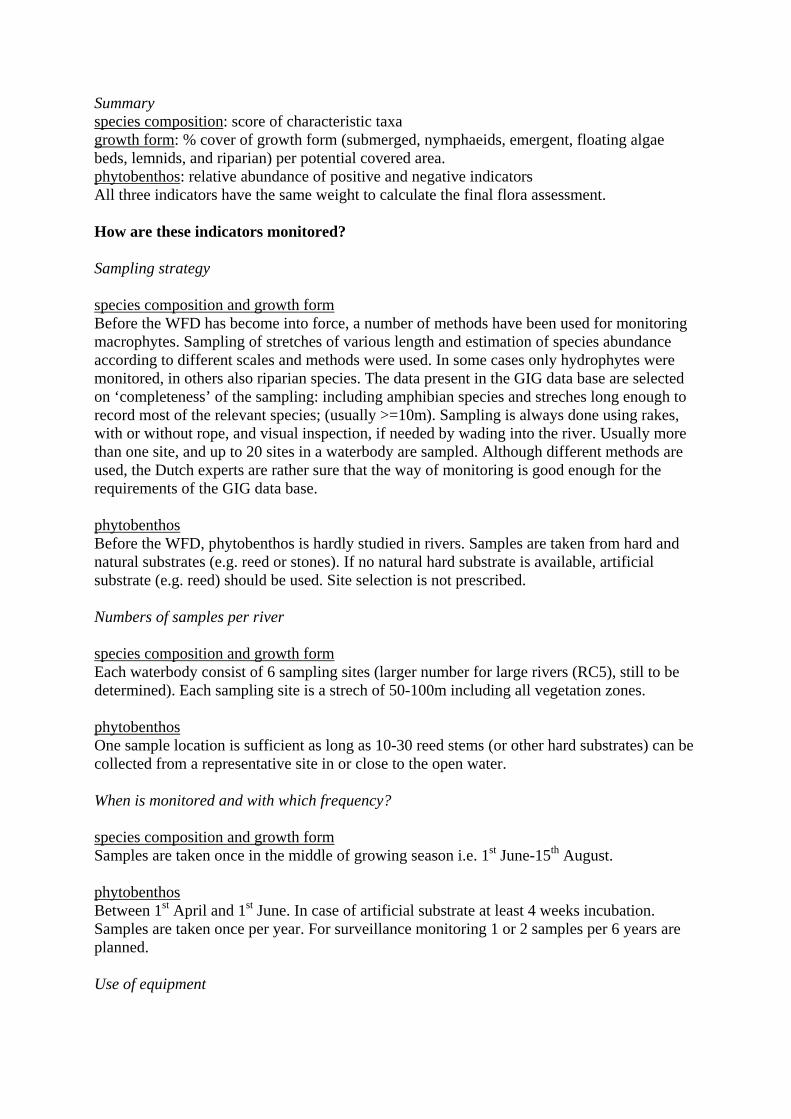
Summary species composition: score of characteristic taxa growth form: % cover of growth form (submerged, nymphaeids, emergent, floating algae beds, lemnids, and riparian) per potential covered area. phytobenthos: relative abundance of positive and negative indicators All three indicators have the same weight to calculate the final flora assessment. How are these indicators monitored? Sampling strategy species composition and growth form Before the WFD has become into force, a number of methods have been used for monitoring macrophytes. Sampling of stretches of various length and estimation of species abundance according to different scales and methods were used. In some cases only hydrophytes were monitored, in others also riparian species. The data present in the GIG data base are selected on ‘completeness’ of the sampling: including amphibian species and streches long enough to record most of the relevant species; (usually >=10m). Sampling is always done using rakes, with or without rope, and visual inspection, if needed by wading into the river. Usually more than one site, and up to 20 sites in a waterbody are sampled. Although different methods are used, the Dutch experts are rather sure that the way of monitoring is good enough for the requirements of the GIG data base. phytobenthos Before the WFD, phytobenthos is hardly studied in rivers. Samples are taken from hard and natural substrates (e.g. reed or stones). If no natural hard substrate is available, artificial substrate (e.g. reed) should be used. Site selection is not prescribed. Numbers of samples per river species composition and growth form Each waterbody consist of 6 sampling sites (larger number for large rivers (RC5), still to be determined). Each sampling site is a strech of 50-100m including all vegetation zones. phytobenthos One sample location is sufficient as long as 10-30 reed stems (or other hard substrates) can be collected from a representative site in or close to the open water. When is monitored and with which frequency? species composition and growth form Samples are taken once in the middle of growing season i.e. 1st June-15th August. phytobenthos Between 1st April and 1st June. In case of artificial substrate at least 4 weeks incubation. Samples are taken once per year. For surveillance monitoring 1 or 2 samples per 6 years are planned. Use of equipment

species composition and growth form For sampling plants in most cases a rake or dredge connected to a rope is used, but smaller rivers are inspected using waders. Sampling bags or jars with alcohol are used for fixation for species determination (mosses, charophytes). phytobenthos Diatoms on the hard substrate are soaked in 10 % HCl. Small jars are used for collection. Analysis of sample and level of determination species composition Most plants are determined to species level in the field, and partly validated in the laboratory. Charophytes and mosses are determined to genus or higher taxa in the field and collected for species determination. phytobenthos Samples are stored frozen and the samples are oxidized (NEN-EN 13946). Determination with microscope (interference/phase contrast) with 100x magnification. 200 shells are determined. Where applicable guidance NEN-EN 13946 Water quality-Guidance standard for the routine sampling and pretreatment of benthic diatoms from rivers and NEN-EN 14407 Water quality - Guidance standard for the identification and enumeration of benthic diatom samples from rivers, and their interpretation, is followed. way of reporting basic data There is not yet a strict procedure for transformation basic data to data ready for assessment. This is planned for June 2007. Assessment Data requirements Species composition The river should be typed and species list should contain a number ranging between 0 and 3 (integer). The GIG database can be used directly, after converting scores 3 to 2 and 4 and 5 to 3. The data of sampling sites have to be consolidated to one list of species with their abundances. For comparability reasons the Dutch samples in the GIG database are only the single site samples from each river that had the highest assessment result with Dutch method. Growth form The rivers should be typed and the growth forms contain a percentage ranging between 0 and 100 of the potential area for each growth form. Phytobenthos Relative contribution of each species to the total should be reported (fraction, %). Table 2. Example of an input file which can be used for automatically calculation of the Dutch macrophyte species metric. In this example 6 site samples of the same waterbody are assessed but also the aggregated samples as a waterbody sample.

Samplenumber 1224 1225 1226 1227 1228 1230 IWaterbody aggregated

watertype R6 R6 R6 R6 R6 R6 R6 Submerged 65 20 80 30 10 40 40 Nympaeids 20 20 10 10 Emergent 10 10 10 5 10 5 8 Lemnids 5 10 10 4 Flab 2 10 5 2 1 2 3 Riparian 90 90 90 90 90 90 90 Agrostis stolonifera 2 2 2 1 Alisma plantago-aquatica 1 1 1 Apium nodiflorum 3 1 Berula erecta 2 1 Bidens frondosa 2 1 1 Carex riparia 2 1 1 Glyceria maxima 2 3 3 1 2 Iris pseudacorus 2 2 1 2 Mentha aquatica 3 1 3 2 Myosotis laxa s. cespitosa 3 1 Myosotis scorpioides 3 1 3 3 2 Persicaria hydropiper 2 3 2 Phalaris arundinacea 3 3 3 2 2 2 Phragmites australis 3 3 3 2 Rorippa amphibia 3 1 1 2 2 Sagittaria sagittifolia 3 2 2 2 2 Scirpus sylvaticus 1 1 Sparganium erectum 2 3 1 2 Stachys palustris 3 1 Symphytum officinale 1 1 Veronica catenata 1 1 Zygmales species 2 3 3 2 Lemna minor 3 3 2 Lemna minuta 3 3 2 2 2 3 3 Callitriche obtusangula 3 3 3 2 Callitriche platycarpa 3 2 3 2 Callitriche species 3 1 2 Elodea canadensis 2 1 Elodea nuttallii 3 2 2 Nitella flexilis 1 1 Potamogeton pectinatus 3 2 2 Potamogeton perfoliatus 3 1 Potamogeton trichoides 3 1 Ranunculus fluitans 3 3 2 Sagittaria sagittifolia f. vallisneriifolia 2 3 2 Sparganium emersum 3 3 3 3 3 3 Juncus effusus 1 1 1 Lythrum salicaria 1 1 Persicaria amphibia 1 1 Potamogeton natans 3 2 2 Rumex hydrolapathum 1 1 2 1 1 1

Methods of calculation <provide way of calculation including weights, groups of species etc provide an example (may be fictive)> species composition

For each type a list with species scores is constructed based on the expected abundance in reference conditions (Annex B). For assessment all scores are summed and compared to the reference score. All class boundaries are also expressed as percentage of the reference score. H/G: 70% G/M:40%; M/P:20% P/B:10%. The boundary percentages are transformed to EQR values, where H/G equals 0.8 and G/M equals 0.6 etc. Table 3. The type specific reference score (R5, R10, R12, R14, R18 = R-C1; R6, R15 = R-C4; R7, R8, R16 = R-C5). Type R5 R6 R7 R8 R10 R12 R14 R15 R16 R18 Referentiescore 41 64 40 38 43 60 33 26 15 35 Table 4. An example for calculation of species metric for a R6 type river. Species in the lake Abundance (0-3) Score (see ANNEX B) Agrostis stolonifera 2 1 Alisma plantago-aquatica 1 1 Callitriche obtusangula 3 - Glyceria maxima 3 0 Iris pseudacorus 2 1 Juncus effusus 1 - Lemna minuta 2 - Lythrum salicaria 1 1 Myosotis scorpioides 3 1 Phalaris arundinacea 2 1 Ranunculus fluitans 3 4 Rorippa amphibia 1 1 Rumex hydrolapathum 1 1 Sagittaria sagittifolia 2 2 Sparganium emersum 3 3 Sparganium erectum 1 1 Symphytum officinale 1 - Calculation: 1. Sum of scores = 18, reference score= 64 (see table 3) 2. EQR not transformed: 18/64=0,281 or 28.1 % of the ref score meaning Moderate 3. EQR transformed (for averaging): linear transformation within class boundaries 0.4

and 0.6 (20% and 40%) gives: 0.481 (half way moderate).

Growth form From the basic data one number for each growth form is aggregated. Example: the channel of a river of type R5 (RC1) is covered by submerged macrophytes at both sides, for 20% of the channel width, but consistently over a long stretch. The potential area is channel wide because is it maximum 1,4 m deep. The covered area is 20%, or ‘good’ status (exactly on G/M boundary, see ANNEX A). Principle of transformed EQR is the same as for species metric; in this example: 0,6

Phytobenthos For a sample the share of ‘positive’ and ‘negative’ individuals is determined as compared to the total presence of diatoms (some species are indifferent). The species are listed in ANNEX C and the boundaries with critical share of negative species in Table 5. The correlation between quality status and share of positive species was unclear in preliminary studies and there not yet considered in the calculation. Example: The sum of relative abundances of positive species appears 5% and the share of negative species 20%. For the negative species status is the status mid Moderate (see Table 5) with transformed EQR of 0.45. Principle of transformed EQR is the same as for species metric.

Table 5. Boundaries for percentages of negative and positive species of Diatoms. The species listed as ‘positive’ or ‘negative’ are listed in ANNEX C.

Satus Percentage negative species EQR High (mid) 2,5 0.9 High/Good 5 0.8 Good/Moderate 10 0.6 Moderate/Poor 30 0.4 Poor/Bad 50 0.2

How are reference conditions, H/G and G/M boundaries derived? The number of reference sites is too low for setting reference values. The reference for species composition is based on the idea of having complete plant communities in reference conditions. The list of plant communities that are considered to be present in reference conditions is based on earlier work on target types in nature management (Bal et al.) and improved by expert judgedment. Vegetation data from the database on well developed plant communities in The Netherlands (Schaminée et al.) is used to list all characteristic and all frequent (>20% occurrence on relevé basis) species of these plant communities. The weight given to species at the three abundance levels is derived from both the plant communities charactistics and expert judgment. The reference score for the sum of the scores of the species is derived from frequency data in the vegetation database, which is considered a good estimate for the probability of finding the species in a fixed amount of samples. The fraction of species (or EQR or deviation from reference) at G/M and H/G are estimated with expert judgment, and adjustment may be needed because of too low number of reference sites. Final adjustment of the reference scores are based on intercalibration results. The potential area where macrophytes can grow relies also on expert judgment. The selection of positive and negative diatoms is based on both literature and expert judgment. The boundary percentages are derived purely on expert judgment. How well correlate the indicators with pressure indicators? The species indicator is correlating with hydromorphological pressures and eutrophication. The selection of the species and their weight has been done on there indication value for these pressures. No tests have been done to check the correlation between assessment results and pressure data yet. How is dealt with differences between national data and assessment vs. GIG data and assessment?

Completeness of method The Dutch method uses species composition and growth forms cover for macrophyte assessment, both of which contribute equally to the final assessment. In the GIG comparison only the species composition metric has been used because the data needed for the growth form metric is missing in the GIG database. Data transformation to GIG data base Data on species were compatable with the GIG database format, the numerical scale for abundance of the species was converted from 5 class scale to a 3 class scale (1 -> 1 / 2+3 -> 2 / 4+5 -> 3). Some species had to be renamed after their synonyms. Assessment transformation to the GIG data base - The parameters for growth form cover could be derived from species abundance data but accuracy of such a transformation is far too low even for assessment in groups of classes and was therefore not performed; if the species abundance in the GIG data would have been in a 10 class scale or more (best in percentage cover), the transformation could have been performed. - The NL method was designed to assess aggregated water body data (multiple samples combined or areal surveys) rather than assessing individual sites. The assessment is based on tot summarised score of every characteristic species found in these samples, divided by the expected maximum score for reference waterbodies. When applied to individual samples (which are then regarded as extremely small water bodies), the scores are consistently lower than the aggregated scores for water bodies. The original boundaries of the metric were set by expert judgement in 2004. In December 2006 all reference values were recalculated on the basis of a stochastical approach. The expected chance that the species could be found in samples was derived from the database of samples of well developed vegetation in The Netherlands. These new values were lower than the originals based on expert judgement. The estimation of the expected chance to be found in samples was done for every species and for single samples as well as increasing number of multiple samples. The reference scores were set on the summarized chance of species to be found in 5 representative samples from a waterbody. The summarized chance of species to be found in only one of those samples was calculated to get an estimate for the correction needed for the expected maximum score for reference waterbodies, to apply the assessment method for single site samples. The correction factor showed to be +/- 3 for most NL types and is suitable for assessing randomly selected samples. Analyses of the variability was done within site samples of 22 waterbodies from Netherlands completed with multiple site samples of waterbodies from France and UK in the GIG database, both on species richness and on assessment results. These analyses showed that the variability was at least a factor 2 between the minimum and the maximum, both in species richness and in NL-assessment score. The samples from NL added tot the GIG database were the site samples of the selected waterbodies with the highest NL assessment score. Because the difference between mean and maximum was roughly 1.5, the correction factor for single site assessment should be 3/1.5 = 2. It was assumed that the samples provided by the other MS for the GIG database were also best sites of a waterbody and therefore also could be assessed using the correction factor 2. It is very difficult to estimate the confidence boundaries round the correction factor on a sound statistical basis. A crude estimation is that the 90% confidence limits are at +/- 1.3 and 3, which means that the assessment confidence is +/- one quality class.

- Indicator species that do not exist in other MS were excluded from the metric when applied for the samples of those MS, the reference value and class boundaries were corrected accordingly. - Species that do not exist in Dutch but have the same indicator value in other MS were included in the metric when applied for the samples of those MS, the reference value and class boundaries were corrected accordingly. - The last two corrections had almost no effect on the assessment results in comparison to the uncertainty due to the problem encountered with site assessement versus waterbody assessment and therefore eventally not applied. Transformations on national methodology The Dutch method was developed in 2004 with tentative reference values and class boundaries. In comparion with methods of other MS the methods was considered to stringent both for lakes and rivers. December 2006 all reference values were recalculated and from then on the new values were used in the comparisons. For lakes, it became clear from intercalibration results that these new values had to be adjusted another 15%; the values will be adjusted for rivers according to intercalibration results.

ANNEX A. Overview of growth form boundaries (% cover) for each Dutch river type (drijvend=nymphaeids, flab=floating algae beds; kroos=lemnides; oever=amphibious, riparian zone). The left column represent the transformed EQR.

R5 R6 R7 R8 R10 R12 R14 R15 R16 R18

submers 0,0 0 0 0 0 0 0 0 0 0 0 0,2 1 1 0,1 0,5 1 1 1 1 1 1 0,4 5 5 0,5 1 5 5 2 2 5 2 0,6 20 20 1 2 10 10 5 5 10 5 0,8 30 30 5 5 20 20 10 10 20 10 1,0 65 60 20 10 40 40 20 20 30 20 0,8 100 100 100 100 50 50 30 40 100 30 0,6 70 70 50 60 50 0,4 100 100 70 80 70 0,2 100 100 100drijvend 0,0 0 0,2 1 0,4 5 0 0 0,6 10 1 1 0,8 20 5 5 1,0 25 10 10 0,8 50 15 15 0,6 90 30 30 0,4 100 50 50 0,2 80 80 0,0 100 100 emers 0,0 0 0 0 0,2 1 1 1 0,4 3 2 2 0,6 5 5 5 0,8 10 10 10 1,0 20 15 15 0,8 50 20 20 0,6 90 50 50 0,4 100 75 75 0,2 95 95 0,0 100 100 flab 0,8 0 0 0 0 1,0 1 2 2 2 0 0 0 0 0,8 3 5 5 5 1 1 1 1 0,6 10 10 10 10 5 5 5 5 0,4 30 40 30 30 10 10 10 10 0,2 50 70 50 50 50 50 50 50 0,0 100 100 100 100 100 100 100 100kroos 0,8 0 0 0 0 1,0 1 2 2 2 0 0 0 0,8 3 5 5 5 1 1 1 0,6 10 10 10 10 5 5 5 0,4 30 40 30 30 10 10 10 0,2 50 70 50 50 50 50 50 0,0 100 100 100 100 100 100 100oever 0,0 0 0 0 0 0 0 0,2 10 10 2 1 1 1 0,4 20 20 7 20 20 20 0,6 40 40 15 40 40 40 0,8 60 60 25 60 60 60

R5 R6 R7 R8 R10 R12 R14 R15 R16 R18

1,0 80 80 30 80 80 80 0,8 100 100 100 100 100 100

ANNEX B. List of type specific characteristic species (‘soort’) scores. Per type and per species the number should reed as three separate scores, the first for the lowest abundance (1), the second for the intermediate abundance (2), the third for the highest abundance. Example: Alsima gramineum found in abundance class of 3 in type M5 will get a score of 4. The table continues at the next page.

R5 R6 R7 R8 R10 R12 R14 R15 R16 R18 Acorus calamus 111 111 111 110 120 110 110 110 Agrostis stolonifera 111 111 111 111 Alisma gramineum 111 234 122 111 234 234 234 Alisma lanceolatum 111 111 122 111 111 111 110 110 110 Alisma plantago-aquatica 121 123 122 111 111 123 210 110 234 210 Alopecurus geniculatus 111 111 Apium nodiflorum 121 123 134 344 244 244 Berula erecta 111 111 111 110 110 232 232 110 Bolboschoenus maritimus 111 134 Butomus umbellatus 121 123 122 111 120 111 Calamagrostis canescens 111 111 111 Calliergonella cuspidata 111 234 Callitriche cophocarpa 111 Callitriche hamulata 243 344 344 244 244 234 244 Callitriche obtusangula 120 Callitriche platycarpa 121 111 122 111 110 120 210 232 234 232 Callitriche stagnalis 111 Callitriche truncata 111 Caltha palustris 111 234 Caltha palustris subsp. araneosa 134 Cardamine amara 111 Carex acuta 234 123 Carex acutiformis 120 111 Carex paniculata 344 Carex pseudocyperus 111 Carex riparia 123 111 111 Carex vesicaria 344 234 Ceratophyllum demersum 111 111 122 111 110 111 Cicuta virosa 111 111 Eleogiton fluitans 132 Elodea canadensis 132 111 122 110 234 234 232 244 110 232 Elodea nuttallii 111 110 110 110 110 110 110 Epilobium hirsutum 110 111 110 110 Equisetum fluviatile 132 234 111 234 234 110 110 110 Equisetum palustre 111 111 Galium palustre 111 111 111 111 Glyceria fluitans 111 111 122 111 110 110 210 210 111 210 Glyceria maxima 111 110 111 110 110 100 100 100 Glyceria notata 344 244 111 244 Hippuris vulgaris 111 111 111 Hottonia palustris 243 344 344 111 Hydrocharis morsus-ranae 111 100 111 100 100 111 Iris pseudacorus 111 111 111 110 110 110 110 110 Lemna gibba 100 Lemna minor 100 100 100 100 100 Lemna trisulca 234 100 110 111 Ludwigia palustris 132 Luronium natans 132 344 Lycopus europaeus 111 111 111 111 111 110 110 110 Lysimachia thyrsiflora 234 111 344 Lythrum salicaria 110 111 111 Mentha aquatica 111 111 111 111 Myosotis scorpioides 111 111 111 111 111 110 110 111 110 Myriophyllum alterniflorum 243 344 344 244 Myriophyllum spicatum 132 230 122

R5 R6 R7 R8 R10 R12 R14 R15 R16 R18 Myriophyllum verticillatum 111 234 122 111 234 234 232 111 232 Nitella flexilis 344 Nitella mucronata 243 344 122 111 344 344 111 Nuphar lutea 243 230 134 134 100 120 232 232 234 232 Nymphaea alba 234 134 234 344 234 Nymphoides peltata 123 134 111 111 Oenanthe aquatica 121 234 111 110 120 110 110 234 110 Oenanthe fistulosa 111 234 111 234 234 110 110 111 110 Persicaria amphibia 110 111 110 110 111 Persicaria hydropiper 121 234 111 110 110 Persicaria minor 123 123 Persicaria mitis 123 123 Peucedanum palustre 111 111 110 Phalaris arundinacea 111 110 111 110 110 100 100 100 Phragmites australis 111 111 134 110 110 110 110 Potamogeton alpinus 243 344 123 244 244 244 Potamogeton compressus 111 234 122 111 234 234 232 232 111 232 Potamogeton crispus 132 230 122 111 120 110 210 210 111 210 Potamogeton gramineus 344 Potamogeton lucens 121 234 134 134 123 123 244 244 234 244 Potamogeton mucronatus 111 234 122 111 234 234 232 111 232 Potamogeton natans 111 111 122 111 111 111 111 Potamogeton nodosus 134 111 234 Potamogeton pectinatus 121 110 122 111 210 210 111 210 Potamogeton perfoliatus 121 123 122 111 111 244 244 111 244 Potamogeton praelongus 344 344 Potamogeton pusillus 111 110 122 111 110 110 232 232 111 232 Potamogeton trichoides 132 120 Potentilla palustris 234 Ranunculus circinatus 111 111 122 111 111 111 232 232 111 232 Ranunculus flammula 344 Ranunculus fluitans 243 344 134 230 244 244 234 244 Ranunculus hederaceus Ranunculus lingua 234 111 234 Ranunculus ololeucos 123 Ranunculus peltatus 243 134 110 120 244 244 234 244 Ranunculus sceleratus 111 111 Rorippa amphibia 111 110 111 110 110 110 110 110 Rorippa microphylla 111 111 111 110 110 111 110 Rorippa nasturtium-aquaticum 123 244 Rorippa palustris 110 110 Rumex hydrolapathum 111 111 111 110 110 110 110 110 Rumex palustris 111 111 Sagittaria sagittifolia 121 120 122 111 120 120 244 244 111 244 Schoenoplectus lacustris 122 134 111 111 Schoenoplectus pungens 111 Schoenoplectus tabernaemontani 134 Schoenoplectus triqueter 134 Schoenoplectus x carinatus 111 Sium latifolium 111 111 111 110 111 110 110 110 Solanum dulcamara 110 110 Sparganium emersum 243 123 122 123 123 244 244 111 244 Sparganium erectum 121 123 111 110 120 100 100 100 Spirodela polyrhiza 100 100 100 100 Stachys palustris 110 111 110 Stellaria uliginosa 111 Stratiotes aloides 111 111 Thelypteris palustris 234 111 Typha angustifolia 111 111 111 Typha latifolia 111 110 111 110 110 232 232 110 Utricularia vulgaris 111 111 234 234 111 Veronica anagallis-aquatica 121 123 134

R5 R6 R7 R8 R10 R12 R14 R15 R16 R18 Veronica beccabunga 121 123 111 123 244 244 Veronica catenata 121 123 111 123 110 110 Zannichellia palustris 111

ANNEX C. List of type specific positive (P) and negative (N) indicators of phytobenthos

R5 R6 R7 R8 R10 R12 R14 R15 R16 R18

Achnanthes austriaca var. ventricosa P

Achnanthes lanceolata ssp. frequentissima N N N N N N N

Achnanthes oblongella P P

Achnanthidium ventralis P

Amphipleura pellucida P P P

Bacillaria paxillifer N N

Caloneis bacillum P P P P P P

Craticula accomoda N N N N N N N N N N

Cyclostephanos dubius N N

Cyclotella meneghiniana N N N N N N N N N N

Cymbella gracilis P P

Cymbella microcephala P P P P P P P P P P

Diatoma mesodon P P P P P P P P P P

Diatoma vulgaris N N

Epithemia adnata N N

Eunotia exigua N N N N N N N N

Eunotia implicata P P

Eunotia paludosa N N N N N N N N

Eunotia rhomboidea P P

Eunotia subarcuatoides N N N N N N N N

Eunotia tenella P P

Fragilaria arcus P P P P P P P P P P

Fragilaria ulna N N N N N N N N N N

Frustulia rhomboides var. saxonica N N N N N N N N

Gomphonema olivaceum N N

Gomphonema parvulum N N N N N N N N N N

Gomphonema parvulum f. saprophilum N N N N N N N N N N

Gomphonema pseudoaugur N N N N N N N N N N

Gyrosigma acuminatum N N

Lemnicola hungarica N N N N N N N

Luticola dapaliformis N N N N N N N N N N

Meridion circulare P P P P P P P P P P

Navicula angusta P P

Navicula atomus N N N N N N N N N N

Navicula atomus var. excelsa N N N N N N N N N N

Navicula atomus var. permitis N N N N N N N N N N

Navicula festiva N N N N N N N N

Navicula joubaudii N N N N N N N

Navicula minima N N N N N N N N N N

Navicula molestiformis N N N N N N N N N N

Navicula saprophila N N N N N N N N N N

Navicula subminuscula N N N N N N N N N N

Navicula veneta N N N N N N N N N N

Neidium bisulcatum P P

Nitzschia angustiforaminata N N N N N N N N N N

Nitzschia capitellata N N N N N N N N N N

Nitzschia palea N N N N N N N N N N

Nitzschia paleaeformis N N N N N N N N

Nitzschia supralitorea N N

Nitzschia tubicola N N N N N N N N N N

Nitzschia umbonata N N N N N N N N N N

Pinnularia interrupta P P

Pinnularia subcapitata N N N N N N N N

R5 R6 R7 R8 R10 R12 R14 R15 R16 R18

Planothidium delicatulum N N N N N N N

Psammothidium scoticum P P

Sellaphora seminulum N N N N N N N N N N

Skeletonema potamos N N N N N N N

Stauroneis producta N N N N N N N

Staurosirella leptostauron P P P P P

Tabellaria flocculosa P P P P P P P P P P

Tabellaria quadriseptata N N N N N N N N

Assessment methods based on macrophytes POLAND Finally we have our Polish national method for river ecological state assessment based on macrophytes. The method is very much based on the British MTR and is based on the trophic ranking sore. At the moment the method is focused mainly on lowland river types - counterparts of RC-1, RC-4 and RC-5 in intercalibration exercise. Please, note: Polish intercalibration sites belong to lowland high-alkalinity types: RC-1 1.2 and 2.2 RC-4 1.2 and 2.2. During the fieldwork we record every species which is noticed in the river channel “with a naked eye”. They are given the coverage value in 9 point scale. In order to calculate an index (Macrophyte River Index) we use 146 indicative species (marked as 2 in column “Rec”). The rest of the species we marked as 1 even if we normally don’t find them in Poland (e.g. Elodea nuttallii or some other alien species) – once when we find them we will record them!!! Every of 146 indicative species is given two scores:

1. trophic ranking score (L) from 1 (for hypertrophy) to 10 (for oligotrophy); 2. weights value (W) from 1 for species with broad range of tolerance (eurythopic) to 3

for species with very narrow range of tolerance (stenotopic). Both values are independent on the river types (species have the same L and W values in different river types).

MIR value is calculated: 10⋅⋅

⋅⋅=∑∑

ii

iii

PWPWL

MIR

Where: L – trophic ranking score; W – weights value; P – coverage. Different river types have then different reference value and different border values of ecological state classes. In order to indicate reference, ubiquitous and disturbance indicating taxa for intercalibration purposes we used recalculation (applicable only for lowland, high -alkalinity types RC-1 1.2, 2.2 and RC-4 1.2, 2.2):

Trophic

ranking score L

(1-10)

Weight value W (1-3)

Indication in column URD in Template

1 2 1, 2, 3 2

3 4

1, 2, 3 0

5, 6 1 0 5, 6 2, 3 1 7 8 9 10

1, 2, 3 1

In Polish typology we have only four types of lowland rivers according to macrophytes:

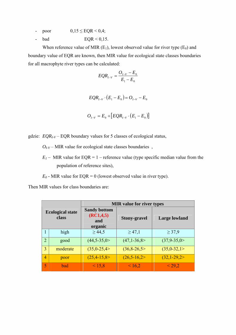
- small and medium-size lowland rivers with sandy bottom; - small and medium-size lowland rivers with gravel and stony substrate; - small and medium-size lowland rivers organic; - large lowland rivers.

Class boundary setting

In order to recalculate MIR index into 1-0 scale the reference value (E1) and the lowest

observed value (E0) of MIR are considered, for different macrophyte river types separately.

The reference value is a median value from reference sites in particular river type.

Then EQRMIR is calculated as follow:

01

0

EEEO

EQRMIR −−

=

where: O –MIR value of the site,

E1 – MIR value for EQR = 1 – reference value (type specific median value from the

population of reference sites),

E0 - MIR value for EQR = 0 (lowest observed value in river type).

In table below reference values and lowest observed values for four Polish macrophyte

lowland river types are given

Macrophyte river types MIR value for EQR =

0 (lowest observed value) (E0)

MIR value for EQR = 1 (median from ref. sites) (E1)

1 Sandy bottom (RC1, 4, 5) 10,0 48,4 2 Gravel-stony substrate 10,0 51,3 3 Organic 10,0 48,4

Large lowland rivers 27,5 39,1

Please, note: in this situation lowland rivers with sandy bottom substrate and lowland organic rivers, although they have different species composition, they have the same MIR values.

In order to set the boundary G/M linear regression was used. Two main indicatiors were

considered:

a) share of natural areas (forests, wetlands) in catchment area;

b) cumulative index of physico-chemical parameters of water quality;

blue – forests and wetlands

red – physico-chemical parameters of water quality (cumulative index)

G/M boundary – MIR = 35

According to statistical analysis boundary values for EQR were proposed as:

- high EQR ≥ 0,9;

- good 0,65 ≤ EQR < 0,9;

- moderate 0,4 ≤ EQR < 0,65;

- poor 0,15 ≤ EQR < 0,4;

- bad EQR < 0,15.

When reference value of MIR (E1), lowest observed value for river type (E0) and

boundary value of EQR are known, then MIR value for ecological state classes boundaries

for all macrophyte river types can be calculated:

01

0

EEEO

EQR VIVI −

−= −

−

( ) 001 EOEEEQR VIVI −=−⋅ −−

( )[ ]010 EEEQREO VIVI −⋅+= −−

gdzie: EQRI-V – EQR boundary values for 5 classes of ecological status,

OI-V – MIR value for ecological state classes boundaries ,

E1 – MIR value for EQR = 1 – reference value (type specific median value from the

population of reference sites),

E0 - MIR value for EQR = 0 (lowest observed value in river type).

Then MIR values for class boundaries are:

MIR value for river types

Ecological state class

Sandy bottom (RC1,4,5)

and organic

Stony-gravel Large lowland

1 high ≥ 44,5 ≥ 47,1 ≥ 37,9

2 good (44,5-35,0> (47,1-36,8> (37,9-35,0>

3 moderate (35,0-25,4> (36,8-26,5> (35,0-32,1>

4 poor (25,4-15,8> (26,5-16,2> (32,1-29,2>

5 bad < 15,8 < 16,2 < 29,2

Centre de Recherche de la Nature, des Forêts et du Bois DIRECTION GENERALE DES RESSOURCES NATURELLES ET DE L

ENVIRONNEMENT

MINISTERE DE LA REGION WALLONNE Av Maréchal Juin 23

B-5030 Gembloux (Belgium) ------------------------------------------------------------------------------------------------------------

Water Framework Directive Intercalibration

Central and Baltic Geographical Intercalibration Group

Macrophytes' method used in BELGIUM (WALLOON REGION) Quality class boundaries for RC3 rivers

Macrophytes' method used in BELGIUM (WALLOON REGION)

The macrophytes' method used in Belgium (Walloon Region) is the Macrophyte Biological Index for rivers (IBMR) –AFNOR, 2003, T90-395. 1.1 Survey Protocol 1.2 Abundance scheme 1.3 Taxonomic basis 1.4 Assessment procedure 1.5 Classification scheme 1.1Survey protocol Field form General description of the station Station coordinates at the downstream point . Conditions of the survey (hydrology (water level), meteorology ,water turbidity) Station length: plant surveys are made generally on 100 meter long stretches, sometimes on 50 meter long stretches in urban or industrial area Station width Dominant lithology of the catchment area Facies number, ( erosive (lotic) or sedimentary (lentic) ) Facies characteristics: rapid, riffle, waterfall, run/glide, pool, slack Facies length Facies width Percentage of each facies in the station Depth of each facies ( 5 classes) Flow velocity ( 5 classes) Shading (5 classes) Substrate (bedrocks, boulders, pebbles, cobbles, gravel, sand, silt, clay, artificial) Vegetalisation -General description -% area covered by the vegetation: vertical projection of the whole vegetation( which cannot exceed 100%) -area free from vegetation on the water surface (%) Floristic composition Cover assessment (%) : -periphyton -heterotroph organisms -bryophytes, -pteridophytes -lichens -algae -angiosperms Total cover can exceed 100% (algae covering the other plants)

Functional composition Cover assessment (%): -Floating hydrophytes and hydrophytes with floating leaves -Submerged hydrophytes -Helophytes Total cover with different vegetal kinds can exceed 100%. Survey protocol Standard ( small and medium size streams wadable ), contact-points ( large rivers) or mixed. Floristic list -All the angiosperms, mosses, liverworts, pteridophytes, lichens, macroalgae and heterotroph organisms growing in the channel are recorded (wet channel ). Area at contact between air and water (tree roots , natural and artificial stones ) is specially explored as previewed in the norma Macrophyte Biologic Index for rivers AFNOR 2003, T90-395 . The survey is made downstream to upstream by wading or by boat ( contact points) The cover of each species ( % of the total superficy) is estimated thanks to a stepwise way . A separate plant list is made for lotic facies and lentic facies . Where the identity of the species cannot be established with confidence in the field, samples are collected for confirmation in laboratory. Samples of bryophytes and macroalgae are systematically collected. Map of the station and the vegetation Location of the station The sampling station is fixed at the end of the waterbody for the monitoring control. 1.2 Abundance scheme Abundance scale :

Cover (%) Scale <0.1 1 ≥0.1 <1 2 ≥1<10 3 ≥10<50 4 ≥50-100 5

1.3 Taxonomic basis Angiosperms, mosses, liverworts, lichens, pteridophytes are determined at the species level. Macroalgae , heterotroph organisms (Sphaerotilus and Leptomitus ) are determined until the genus level, sometimes at the species level when it is possible.

1.4 Assessment procedure The French trophic index (IBMR), a mean of indivual oligotrophic coefficients (from 0 up to 20) weighted by the abundances and the stenoecy coefficients is computed. 1.5 Classification scheme

1.5.1. River-type definition in Wallonia and RC3 type The river-types in Wallonia (Belgium) were defined according to the system B of the Water Framework Directive (criteria: size of the catchment area, slope, five natural regions). The river-type R-C3 (small mid-altitude siliceous type) are the Ardennes brooks (strong and medium slope) and the Ardennes rivers with strong and medium slope. The Ardennes are a natural region which in Belgium only exists in Wallonia . This region extends in France, Luxemburg and Germany. The altitude varies from 300 up to 700 m and its annual average rainfall varies from 1100 mm up to 1400 mm.The annual average temperature varies from 7°C up to 9°C. The geology encompasses Cambrian , Ordovician, Silurian and Eodevonian siliceous rocks .

1.5.2 Reference sites definition Reference sites are selected through two methods. The first one is based on the pressures: • Land use intensification: artificial land-use. Intensive agriculture :<20% of the catchment

area. Cattle breeding :<1,25 animal /ha of the catchment area. • Forestry. Acidification. Eutrophication; • Riparian zone vegetation. • Morphological alterations : adaptation of the French Qualphy method. • Water abstraction. • River flow regulation • Biological pressures:introduction of alien species. • Fisheries and aquaculture . • Biomanipulation. • Recreation uses. Those criteria are observed with only small deviations (mainly for the artificial land-use which often is higher than 0,3%). The second one is based on respect of physico-chemical criteria used for diatoms and macroinvertebrates intercalibration exercise : • N-NO3 ≤average value of 2 mg/l, • O2 : =average value of 95-105% , • N-NH4: ≤average value of 50 microg/l, • P-PO4 : ≤ average value of 20 microg/l • BOD5: ≤average value of 2 mg/l)

1.5.3. Data on reference sites. Reference IBMR value-RC3 rivers Our data set was made up of 29 surveys within which 7 reference sites are considerated ;

IBMR Eau noire 14,15

Alysses 16,83 Rulles 12,72 Ronce 16,07

Masblette 12,47 Basseilles 15,83

Loubas 16,91 Mean 15,00

The value of IBMR used to quantify reference conditions is the arithmetic mean of 7 representative sites (IBMRRef mean: 15,00).The confidence interval -first risk kind: 5% - is included between13,34 and 16,61. Representative sites contain narrow ( 3-5m width) brooks with only bryophytes and average width (5-8m) streams with bryophytes and Ranunculus penicillatus .This explains the medium value (IBMR=15) because Ranunculus penicillatus has a low score (IBMR=12).

1.5.4. Change of the IBMR with the pressure impacts. Setting class boundaries-RC3 rivers. The intercalibration exercise concerns the macrophytes' answer to organic pollution and nutrients. A linear combination of the physico-chemical parameters (N-NO3, N-NH4, P-PO4, BOD5) has been computed (Principal components analysis) to assess the water quality. Most of the variation (52%) is concentrated around the axis one which can be considered as representative of the water degradation. The sites are qualified by their coordinate on axis n°1 (sites scores).

Observations (axes F1 et F2 : 73,35 %)

WAYAI

WARTOISE

WARCHENNE

WARCHEM AL

WARCHEBULL

SALM 06

OURTHEORTHO06OURTHEORI06

OURTHEOCC06

OISE2006

M ACHE

LUVELIENNELORC06

LHOM M EHAT06

LESSELES

LAVAL

HOUILLE 2006

HELLE

ALEINES2006

LIENNEBRAS

BASSEILLES

GILEPPE

LOUBAS STJEAN

M ASBLETTE2006

RONCERULLES

ALISSES

EAU NOIRE

-3

-2

-1

0

1

2

-3 -2 -1 0 1 2 3 4

F1 (52,42 %)

F2 (2

0,93

%)

The graph (IBMR/sites scores) shows a medium relationship ( R2=50%) without obvious discontinuities.

y = -1,2804x + 13,444R2 = 0,5026

0

2

4

6

8

10

12

14

16

18

20

-3,0 -2,0 -1,0 0,0 1,0 2,0 3,0 4,0

Water degradation

IBM

R

The high-good boundary (IBMRHigh:14,25) is set at 95% of the reference value. Data do not cover the whole gradient. Three class boundaries will only be set in total. The lowest value of IBMR in our data set is 7,9 and the class boundary of the high status is 14,25 , so the gradient can be divided into two equal parts to state the limit class of the good/moderate status (IBMRGood/Moderate=11,07) and of the moderate /poor status (IBMRModerate/Poor=7,90).

IBMR Reference value 15,00 High status 14,25 Good/Moderate status 11,07 Moderate/Poor status 7,90

Example of taxonomic composition of the three quality classes (A=abundance).

REFERENCE STATUS GOOD STATUS MODERATE STATUSRiver name-Site Basseilles(Lavacherie) Aleines(Auby/s/Semois) Warche (Bullange)

IBMR score 15.83 12.92 9.20 Phalaris arundinacea

(A=1) Ranunculus fluitans

(A=1) Callitriche hamulata

(A=2)

Ranunculus penicillatus(A=1)

Ranunculus penicillatus (A=4)

AN

GIO

SPER

MS

Petasites hybridus (A=2)

Phalaris arundinacea (A=2)

Leptodictyum riparium (A=1)

Leptodictyum riparium (A=4)

Hyocomium armoricum (A=1)

Platyhypnidium riparoides (A=1)

Platyhypnidium riparoides (A=1)

Pellia epiphylla (A=1) Amblystegium fluviatile(A=3)

Racomitrium aciculare (A=1)

Fontinalis antipyretica (A=1)

Fontinalis antipyretica (A=1)

Brachytecium rivulare (A=1)

Scapania undulata (A=3)

Chiloscyphus polyanthos (A=3)

Fontinalis squamosa (A=3)

Fontinalis squamosa (A=3)

BR

YO

PHY

TES

Thamnobryum alopecurum (A=1)

Lemanea fluviatilis(A=3)

Lemanea fluviatilis (A=1)

Microspora amoena (A=3)

Oscillatoria sp (A=3) Oscillatoria sp (A=2)

Ulothrix zonata (A=1)

MA

CR

OA

LGA

E

Vaucheria sp(A=1) Vaucheria sp(A=1)

INTERIM REPORT JUNE 2006 Summary of approach used in LEAFPACS for defining ecological quality of rivers and lakes using macrophyte composition. Nigel Willby1, John Hilton2, Jo-Anne Pitt3, Geoff Phillips3 1School of Biological and Environmental Science, University of Stirling 2Centre for Ecology & Hydrology, Dorset 3 Environment Agency, Ecology Technical Team Introduction In preparation for the implementation of the Water Framework Directive (WFD), the UK regulatory agencies have commissioned an R & D project to develop a method to classify the ecological status of rivers and lakes on the basis of macrophyte communities. This has become generally known as the LEAFPACS project. Large existing national data sets have been used in the development of the approach described below. It should be borne in mind that the approach described and the resulting classifications require further testing on independent data sets, although a preliminary comparison of outputs for lakes using new data appears to give a good relationship with other parameters such as chlorophyll and total phosphorus. Application of the classification system by the UK agencies may also require the development of additional rules to augment the “raw” classification output from LEAFPACS which currently focuses on macrophyte composition. For example, a complementary method is being developed to deal with macrophyte abundance in lakes. It is anticipated that validation and testing of the system will continue in the light of comparisons with other European methods through the intercalibration process, and as a result of applying the system to new data sets collected by the UK agencies over the last two years. This report is primarily concerned with reporting recent developments relating to the classification of rivers. However, this work has been built on the initial thinking that was developed by working with UK lake data, and reference is made to examples from this work as well. A full report detailing both river and lake classification methods will be produced at the end of the current project (March 2007). The LEAFPACS approach The general approach adopted by the project has been to make use of existing data, for both rivers and lakes, in developing prototype classification tools, which can then be tested using independent data sets. This approach was considered pragmatic given the timescale involved, but the use of existing data, collected by a range of organisations for different purposes, presented a number of difficulties. For rivers, the LEAFPACS project had access to data from c.7000 surveys of river macrophytes collected across Britain and Ireland. Surveys were generally based on one of two methods: Mean Trophic Rank, 100m reach, nine point cover scale, or JNCC, pair of 500m reaches, three point cover scale). The surveys were generally not linked to routine environmental monitoring data, and were not screened to distinguish reference or impacted sites. Surveys included >900 taxa, many of which were either incidental to rivers or wholly terrestrial. Linking of surveys to available environmental and geographical scale data was undertaken by CEH Dorset. This generated sufficient data for intrinsic variables (such as catchment area, slope, distance to source, and

altitude at site or source), but exposed significant gaps in the match to pressure variables such as nutrients, which at initial inspection were most readily available for the most impacted sites. The approach used by the LEAFPACS project was a pragmatic solution to the above challenges. The key stages can be considered as follows:

1. Establish an environmentally based typology for the water category 2. Derive a metric that can be used to assess sensitivity of the biological quality element to a

pressure 3. Develop a rationale for placement of boundaries between classes across the range of

metric values 4. Screen sites on a type specific basis to identify putative reference sites 5. Develop a method for prediction of site specific reference conditions using widely

available environmental data 6. Convert a site metric to an EQR to allow WFD compliant site classification

Two further areas that are developed in this report are the derivation of nutrient standards for macrophytes in rivers and the issue of uncertainty in classification due to sampling variability. 1. An environmentally-based typology for river macrophytes. Holmes et al. (1999) produced a TWINSPAN based classification of river macrophyte data from c.2200 sites, widely distributed across the UK. The surveys on which the classification was based were not exclusively of high or good quality sites (although they were largely initiated by statutory conservation agencies for site assessment), indeed several classes of sites were considered to be characterized by a high level of human influence. The relationship between this biological classification and intrinsic environmental variables formed the basis for defining an environmental typology in the present project. It is important to realize that the typology developed here is a means to an end, not an end in itself - it is an important step in screening a large population of sites for sites that could be considered as being in reference condition. The 16-type classification used by Holmes et al (Types I-IV plus the classification in which each of the remaining six types are split once) was analysed using discriminant analysis and CCA of the compositional data on which the classification was based. These analyses highlighted the overriding importance of slope and geologically-based variables (such as alkalinity or composition of drift geology) in driving variation in macrophyte composition. The boxplots in Figure 1 illustrate the relationship between these variables and the distribution of sites in the various biological types. On the basis of these figures four alkalinity classes and four slope classes were defined. Several alternative sets of values were trialled, but an analysis of the distribution of biological types between environmental types indicated that these classes resulted in the least random distribution of biological classes across environmental classes. Through aggregation of three of the least populated types in a 4 x 4 matrix of alkalinity x slope, a 13 celled typology was achieved. The environmental typology in Table 1 has formed the basis for all subsequent analysis. It should be noted that discrete separation of biology in relation to environment is not expected, partly because some biological types are inherently impacted (and will therefore overlap with unimpacted assemblages sharing the same combination of slope and alkalinity), partly because a range of biological types might naturally be expected for a given environmental type even under reference condition, and partly because a combination of other environmental variables (e.g. shading and substrate) will explain background variation in assemblages.

2

Ia-cIIa-c

IIIa-bIVa-c

Va-cVd-e

VIa-cVId-e

VIIa-bVIIc-d

VIIIa-cVIIId-e

IXa IXb-cXa-b

Xc-e

holmes type

0.00

0.50

1.00

1.50

2.00

2.50

3.00

log

alka

linity

(mg/

l CaC

O3)

Ia-cIIa-c

IIIa-bIVa-c

Va-cVd-e

VIa-cVId-e

VIIa-bVIIc-d

VIIIa-cVIIId-e

IXa IXb-cXa-b

Xc-e

holmes type

-1

0

1

2

log

slop

e (m

/km

)

Figure 1. Distribution of Holmes et al. (1999) 16 river biological types in relation to alkalinity (derived from matched chemistry data) and reach slope. The y axis is stratified to indicate the optimal thresholds for each variable.

3

Table 1. Environmental typology of UK rivers based on variation in macrophyte composition. Figures are numbers of sites, italicized figures are numbers as a percentage of the total

Gentle Low Moderate Steep(<1) (1-3) (3-8) (>8)

Low 154 350 617(<10) 3.8 8.5 15.1

Moderate 241 277 817(10-50) 5.9 6.8 19.9High 430 538 370 296 1634

(50-200) 10.5 13.1 9.0 7.2 39.9Very high 485 388 1031

(>200) 11.8 9.5 25.21327 926 923 923 409932.4 22.6 22.5 22.5

Alk

alin

ity (m

gl-1

CaC

O3)

Slope (mkm-1)

1132.82997.3

1583.9

2. Deriving a metric for pressure assessment The evidence from analyses of species richness and total cover is that these variables in rivers are poorly correlated with nutrient enrichment pressures, and therefore cannot be used to classify ecological status with any meaningful confidence. Richness is sensitive to survey method, surveyor experience and inconsistencies over bank vs. channel limits to recording. Cover is notoriously variable, depending on factors such as shade or substrate (that are not routinely or systematically recorded), or antecedent flow conditions. In lakes, it is difficult to derive a measure of total cover of macrophytes from community data scored on a DAFOR scale. Maximum depth of rooting would be a far more useful measure but is currently only available for a minority of lakes in the UK. Initial analyses indicate that the frequency distribution of macrophyte cover scores is sensitive to nutrient enrichment and that this could be used to develop an abundance-based metric for use in lakes. At the present time the LEAFPACS approach is based solely on community level metrics. Calculation of a pressure metric using the global populations of sites and biological data:

One approach to this, based on reciprocal averaging of expert-derived species ranks for a perceived pressure has been used for macrophytes. This approach was first applied to quadrat data collected as part of the UK’s Countryside Survey 2000, to allow an adjustment of continental Ellenberg indicator scores for British plant taxa, and is described in detail in Hill et al. (2001). The mechanics of applying this method are given in Appendix 1.

•

•

•

In essence this method examines the relative abundance of a large suite of species across a large number of sites, and re-defines “expert scores” such that biological and ‘environmental’ datasets are optimally correlated. There is no absolute necessity to perform this step in order to follow the process described below if a suitable expert ranking is already available, but experience to date suggests that expert scores are rarely consistently aligned across species for the pressure or environmental gradient they are designed to reflect.

4

Using this method it is also possible to define ranks for species that were originally unranked by the expert system, and to calculate a measure of tolerance associated with each species rank that can be used as a measure of its indicator value.

•

•

•

•

•

•

•

•

This approach can be used within intercalibration to allow national methods developed in countries from which certain species are absent or unrecorded to be applied to a common dataset. Missing scores can be calculated as detailed in the Appendix whereby these scores are contingent upon the scores of those species for which values are already available. Note that in such a case the original scores could be expert derived or based on, for example, empirical nutrient optima.

This approach may be most appropriate when there is a very large biological dataset but the necessary environmental data are either missing, unevenly distributed (in relation to type or perceived class), or inappropriate to describe a pressure from the perspective of the biological quality element (e.g. water column rather than sediment interstitial nutrient concentrations, spot not monthly samples, a particular fraction not loading).

When the appropriate environmental data do exist, care should be taken to ensure that it is valid to scale up from regional studies (where such data are more likely to exist) to larger scales, and that the niche of rare, but locally abundant species is both adequately described and consistent with the autecological information on such species. In other datasets, such as those that exist for phytoplankton, sufficient direct measurements of a relevant pressure well matched to biological data should exist for the species optima to be determined in relation to an empirical gradient (this could be for individual nutrients or a synthetic gradient combining N, P and chlorophyll a). Cosmopolitan species distributions and widely distributed sampling may render concerns over rare species and scaling less relevant for some quality elements.

Once species scores have been derived they are used to calculate site index scores (see Appendix 1) 2.1 Ground truthing site index scores. Examine the relationship between the site index scores and a suitable indicator of the pressure to which the species ranks are designed to be sensitive.

Since a later stage of the process may involve the use of such relationships to derive regulatory values for physicochemical variables to support high or good ecological status, it is obviously desirable for such relationships to be strong and to be improved by the use of adjusted species ranks relative to the original expert version. An example of testing vegetation-based site scores against spot summer TP values in Northern Irish lakes is shown below (Figure 2). Given that part of the rationale for biological indicator scores is that they reflect environmental determinants of species distribution that cannot, or cannot readily, be measured directly, it is difficult to falsify species ranks, although it is possible to partition and test their underlying environmental basis. It should be noted that a perfect correlation between biology and pressure is not the target of this exercise since the role of biology in monitoring would then become largely redundant. Experience suggests than an r2 of about 0.60 is the maximum that can be achieved.

A second stage in assessing the utility of the new site scores is to include this as a supplementary variable in an ordination of biological data that is constrained by available environmental data.

5

An example of this is shown below (Figure 3) by a CCA analysis of macrophyte composition for 1250 lakes in the REBECCA lake dataset (data supplied and managed by Bernard Dudley, CEH). The environmental variables retained are the minimum necessary to explain significant variation in the species data. The Lake Macrophyte Nutrient Index (LMNI) has been supplied as a supplementary variable to illustrate the strength of correlation with chlorophyll and phosphorus and its general utility as an aggregative measure of enrichment pressure.

•

unrefined scores

R2 = 0.19

1

1.5

2

2.5

3

3.5

4

1 3 5 7 9

lake TR

log

summer

TP

(ugl1)

unrefined scores

R2 = 0.19

1

1.5

2

2.5

3

3.5

4

1 3 5 7 9

lake TR

log

summer

TP

(ugl1)

algorithmic adjustment

R2 = 0.33

1

1.5

2

2.5

3

3.5

4

1 3 5 7

LMNI

log

summer

TP

(ugl1)

9

algorithmic adjustment

R2 = 0.33

1

1.5

2

2.5

3

3.5

4

1 3 5 7

LMNI

log

summer

TP

(ugl1)

9

Figure 2: Relationship between site index scores and pressure. “Unrefined” scores are derived using the lake Trophic Rank expert score system developed by Palmer et al (1992). LMNI = Lake Macrophyte Nutrient Index developed using the LEAFPACS approach, and applied to the same population of sites.

-2.0 3.0

-1.5

1.5

Alt

Alkal

logAlkal

logChlorlogColour

logSRP

logTNlogTP

LMNI

UK

Ee

Fi

LT

LV

NL

NOPL

RO

Figure 3: CCA analysis of lake macrophyte data (REBECCA European data set). LMNI is fitted as a supplementary variable. Grey triangles represent centroids of data supplied by different countries.

6

3. Developing a rationale for boundary placement The protocol for class boundary placement, and identification of reference conditions, for both lakes and rivers using macrophyte composition, is based on thresholds in the relative cover of groups of species that show similar or contrasting responses to a pressure gradient. For example, the switch between positively and negatively responding species is regarded as critical, and could represent the mid-point of moderate class. The switch from high to good status may occur where strongly negatively responding species become subordinate to positively responding ones. It is then possible to stratify the pressure gradient (whether measured or inferred) in an objective and defensible (albeit still arbitrary) way. This is illustrated in Figure 4 below, using macrophyte data from low gradient, base-poor rivers as the example. A prerequisite of this approach is clearly the ability to classify species into different response groups.

Type 1

0

0.1

0.20.3

0.4

0.5

0.6

0.70.8

0.9

1

2.0 3.0 4.0 5.0 6.0 7.0 8.0 9.0

RMNI

rela

tive

cove

r

strong negativepositivecombined negative

HIGH GOOD POOR Figure 4: Potential class boundaries inferred from the changes in relative cover of species identified as responding negatively and positively to a pressure gradient. RMNI – River Macrophyte Nutrient Index. The arrowed line indicates the median of the High class and is considered to equate to an EQR of 1.0. Any approach to classification involves some element of subjectivity, whether in the rules devised, the choice of analytical method, or the interpretation of analytical results. The approach outlined here shows where the subjectivity lies and imposes it consistently. In this sense it does not claim to be right or wrong, it is simply one of several possible approaches that can be evaluated on their merits, but it is suitable for dealing with data whose characteristics present challenges to the use of other approaches. This approach ought to be usable by anyone on any dataset, if equipped with CANOCO 4.5 and SPSS, or software with similar capabilities. A particular feature of the present approach is that reference sites are identified based on their biology rather than the view of regional experts or screening sites by pressures (Figure 5). Thus the basis of the biological approach is:

BADMOD

Type 1

0

0.1

0.20.3

0.4

0.5

0.6

0.70.8

0.9

1

2.0 3.0 4.0 5.0 6.0 7.0 8.0 9.0

RMNI

rela

tive

cove

r

strong negativepositivecombined negative

HIGH GOOD POORMOD BAD

7

(i) the response of individual species to pressures as indicated by empirical data or expert view;

(ii) knowledge of species associations based on empirical data; (iii) use of historical records to either validate the benchmark indicated by contemporary

data or, if necessary, to set a new (unimpacted) benchmark. While the site-based approach has advantages the screening rules are themselves only best judgment, often based on understanding of a limited number of biological quality elements. Hence they may not be equally suitable for all quality elements, and to be applied widely also require the full complement of pressure data to be available for all sites. Unfortunately such pressure data is not universally available for contemporary biological survey data, since monitoring is generally concentrated at impacted sites to check compliance. Even the use of catchment land use to assess potential nutrient loading requires these data to be both available and, for site locations, to be readily resolvable within a GIS framework in order for such data to be extracted. The requirement for direct pressure data also normally precludes the use of historical biological data which may ultimately provide the best indication of reference conditions. A further weakness of this approach is that the derivation of supporting standards for biology at class boundaries is essentially circular since a prejudgment was made on this when selecting reference sites at the outset.

Pool of sites x physicochem

Reference sites

Reference biology

Pool of sites x biology

Reference biology

Reference sites

Figure 5. Approaches to identification of reference sites from an initial large site pool. The first method relies on a large pool of environmental data that can be used for screening pressures plus an understanding of how the biology responds to these pressures in order to set appropriate pressure thresholds. The second method requires an understanding of autecological behavour of individual species, species associations and a historical benchmark of reference biology. 3.1 Identifying members of response groups. 1. Using site scores calculated from cover or abundance-weighted species scores (as in 2 above)

as the environmental variable, perform a CCA on a (lake or river) type-specific basis, with

8

the site x biological data for that type as the dependent dataset. This allows members of response groups to be identified appropriate to each water body type, rather than imposing an arbitrary grouping based on the original species ranks that would not be appropriate to all types. For example, if macrophyte species ranks lie on a continuous scale from 1 to 10, regarding all species with ranks of 1-3 as always being strongly negatively responding and those with ranks >7 as always positively responding may be appropriate to base-poor, upland rivers, but would be inappropriate for lowland base-rich rivers where site scores typically exceed 7 and species characteristic of very nutrient poor conditions are naturally absent.

2. Prepare a table for each river or lake type from the CCA solution file of CCA axis 1 species

scores, tolerance values associated with these scores, sample sizes for each species and the derived expert scores for those species that were generated from an analysis of the global dataset in step 1. Examine the trend in species scores in relation to their global rank to determine whether high scores are associated with high or low ranks (this will vary arbitrarily between types as a function of the analysis). Prepare a separate column combining the species score and its tolerance. If high scores are associated with high ranks then the tolerance value should be added to the site score while if high scores are associated with low ranks the tolerance should be subtracted from the species score.

3. The rationale for classifying species into different response groups is that when species

scores switch from negative to positive they change from being overall negative to positive responders on the inferred pressure gradient. This point must coincide with the centroid of the site scores included in the analysis. To separate strongly negatively responding species (SNRs), that are considered to be characteristic of type specific reference conditions, from negatively responding species (NRs) that ultimately decline along a pressure gradient but are stimulated by a low level of pressure, the species score + tolerance is used. When this value exceeds zero it is considered that species are no longer SNRs since their tolerance ‘carries’ them into potentially impacted sites.

4. When the number of samples containing a species is small (<10), its distribution at a type-

specific level may be a poor guide to its ecological affinities. For example, a globally high ranking species that, by chance, within a type occurs at three sites dominated by SNR species, cannot be taken reliably to also be a SNR. Similarly, because a species with a low rank, that is an SNR in other types where it is better represented, happens to occur at a few high scoring sites with positive responders (PRs) this does not indicate reliably that this species is also a PR. Consequently, when species are rare in a type their classification is defined by their global rank. The values to be used are defined by regressing the site scores, or site score+tolerance, against the global rank for the more frequent species in that type (>10 records), with the critical values being given by the intercept on the y axis.

5. Therefore, in the prepared table, sort by sample size and allocate species present in <10

samples to SNR, NR or PR groups based on their global rank, using the thresholds determined in (4) above. For the more frequent species sort by species score to separate NRs and PRs, using a cut-off value of zero. Within NRs sort by species score + tolerance to separate SNRs from NRs, using a cut-off value of zero.

The diagram below (Figure 6) illustrates the species scores from a CCA analysis of one river type, ranked in ascending order, with tolerance values and classification of species into response groups. Species that outlie the main zones of the different response groups have been classified on the basis of their global rank rather than the type specific ordination. Note

9

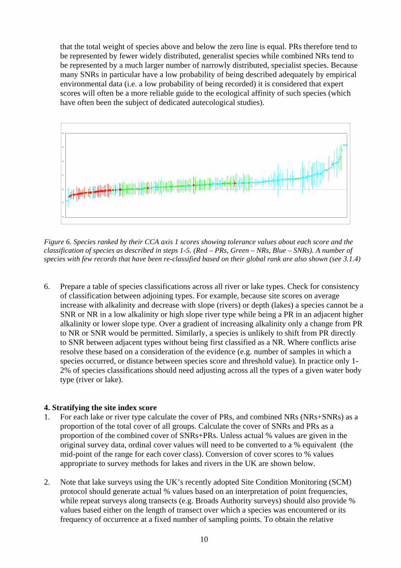
that the total weight of species above and below the zero line is equal. PRs therefore tend to be represented by fewer widely distributed, generalist species while combined NRs tend to be represented by a much larger number of narrowly distributed, specialist species. Because many SNRs in particular have a low probability of being described adequately by empirical environmental data (i.e. a low probability of being recorded) it is considered that expert scores will often be a more reliable guide to the ecological affinity of such species (which have often been the subject of dedicated autecological studies).

-4-2

02

46

8

Figure 6. Species ranked by their CCA axis 1 scores showing tolerance values about each score and the classification of species as described in steps 1-5. (Red – PRs, Green – NRs, Blue – SNRs). A number of species with few records that have been re-classified based on their global rank are also shown (see 3.1.4)

6. Prepare a table of species classifications across all river or lake types. Check for consistency of classification between adjoining types. For example, because site scores on average increase with alkalinity and decrease with slope (rivers) or depth (lakes) a species cannot be a SNR or NR in a low alkalinity or high slope river type while being a PR in an adjacent higher alkalinity or lower slope type. Over a gradient of increasing alkalinity only a change from PR to NR or SNR would be permitted. Similarly, a species is unlikely to shift from PR directly to SNR between adjacent types without being first classified as a NR. Where conflicts arise resolve these based on a consideration of the evidence (e.g. number of samples in which a species occurred, or distance between species score and threshold value). In practice only 1-2% of species classifications should need adjusting across all the types of a given water body type (river or lake).

4. Stratifying the site index score 1. For each lake or river type calculate the cover of PRs, and combined NRs (NRs+SNRs) as a

proportion of the total cover of all groups. Calculate the cover of SNRs and PRs as a proportion of the combined cover of SNRs+PRs. Unless actual % values are given in the original survey data, ordinal cover values will need to be converted to a % equivalent (the mid-point of the range for each cover class). Conversion of cover scores to % values appropriate to survey methods for lakes and rivers in the UK are shown below.

2. Note that lake surveys using the UK’s recently adopted Site Condition Monitoring (SCM)

protocol should generate actual % values based on an interpretation of point frequencies, while repeat surveys along transects (e.g. Broads Authority surveys) should also provide % values based either on the length of transect over which a species was encountered or its frequency of occurrence at a fixed number of sampling points. To obtain the relative

10

abundance of the different response groups sum the derived cover for the species belonging to each response group and then divide by the cover or frequency of all groups combined.

Table 2: Standard conversion of cover scores to percentage cover values for UK lakes and rivers

Lake cover score

% equivalent River cover score

% equivalent

1 1 1 (1) 0.05 2 5 2 0.5 3 10 3 (2) 1.7 4 25 4 3.8 5 50 5 7.5 6 (3) 17.5 7 37.5 8 62.5 9 87.5

Bracketed values in river cover scores refer to cover scores used in JNCC survey method (Holmes et al., 1999). 3. The purpose of classifying species into response groups is merely to enable a stratification

of site index scores that is consistent with WFD normative definitions. Therefore, model the distribution of relative cover values for different response groups across the site index scores for the population of sites in that type. Appropriate techniques are logistic regression with an upper bound of 1, or logistic regression with a Gaussian link function. See Figure 5 below. Note the standard error associated with each model. This is typically in the region of an absolute relative % cover value of 10-15%.

4. Using the fitted values from these regressions and the error value, identify the point on the

site index score where %PRs = %combined NRs, and the upper and lower index scores equivalent to this cross-over point plus or minus the error value.

If the change from dominance by NRs to PRs is regarded as an undesirable change and a significant distortion in composition compared to good ecological status (as described in the WFD normative definitions), it is appropriate to regard this crossover as the middle of the moderate status class.

•

•

•

•

•

At this point minus its standard error the probability of an undesirable impact is low (i.e. it is relatively improbable that cover of PRs will exceed the cover of combined NRs), and this is therefore appropriate for the G/M boundary as directed in the ECOSTAT Guidance on Eutrophication. Conversely, at the crossover point plus its standard error the probability of an undesirable impact is high (i.e. it is relatively likely that cover of PRs will exceed that of combined NRs), and this is therefore an appropriate point for the M/P boundary. The H/G boundary is defined by an index score equivalent to the crossover in cover of SNRs and PRs (relative to the combined cover of these groups on their own) minus the error associated with this point. At this site index score the relative cover of SNRs typically exceeds PRs by two to –three-fold. A total absence of PRs from reference sites is not an appropriate goal since such species are often present as subordinates in unimpacted assemblages. The interpretation of the H/G boundary is more esoteric compared to G/M and M/P boundaries but this threshold has been found to be appropriate for capturing known

11

reference sites defined from palaeo-ecological or historical archive data, or contemporary examples from catchments free from pressures.

It should be noted that while the concept of crossover points is beguiling they are merely a self fulfilling prophecy of the analysis.

Figure 7: Distribution of different response groups across the range of River Macrophyte Nutrient Index site scores for “Type 3” rivers. 5. The threshold values for the pressure metric (in this case RMNI) should then be examined

(Table 3) and the candidate reference sites checked as described below. The overall proportion of sites classed as being in reference condition was 17% but it can be seen from Table 3 that this varied widely between types (from 46% in Type 3 to <4% in Types 11 and 12).

5. Assumptions and verification of reference species and sites One key assumption in classifying species in this way is that sites within a type cover the full gradient from ‘pristine’ to highly degraded. If this is not the case and the gradient in quality is truncated (e.g. there are no minimally impacted sites or no severely impacted sites), a gradient in species distribution will still emerge, but the species classification that results will not be appropriate for stratifying site scores in a way that is consistent with WFD normative definitions.

12

One way to determine whether populations of sites in different types cover a similar gradient of impact is to check that the scores associated with thresholds of change in the relative cover of different groups show a consistent pattern of change (direction and magnitude), both from one type to another, and within a type in relation to the position of the G/M boundary relative to the H/G boundary. For example, modelled scores must increase moving from one type to another where types are distinguished on the basis of increasing alkalinity, and decrease from one type to another where sites are distinguished on the basis of increasing slope (rivers) or depth (lakes). This is illustrated in Table 3. Table 3: Modelled River Macrophyte Nutrient Index scores for different river types at the class boundaries

n n ref median H H/G G/M M/P P/BLowAlk, Low Grdt 120 32 3.65 3.99 4.53 5.13 5.99LowAlk, Mod Grdt 154 39 3.23 3.82 4.47 5.04 5.79LowAlk, High Grdt 360 167 3.24 3.8 4.28 4.78 5.38ModAlk, Low Grdt 365 104 5.13 5.49 5.77 6.25 6.85ModAlk, Mod Grdt 299 74 4.75 5.04 5.42 5.95 6.64ModAlk, High Grdt 298 87 4.23 4.65 5.21 5.75 6.46HighAlk, Vlow Grdt 726 86 6.25 6.59 7.05 7.49 8.06HighAlk, Low Grdt 975 159 5.95 6.39 6.77 7.17 7.68HighAlk, Mod Grdt 554 157 5.58 6.13 6.64 7.1 7.67HighAlk, High Grdt 319 73 4.62 5.12 5.91 6.37 6.96VHighAlk, Vlow Grdt 1040 26 6.78 6.98 7.51 7.88 8.36VHighAlk, Low Grdt 793 32 6.53 6.85 7.35 7.7 8.15VHighAlk, Mod Grdt 276 22 6.01 6.51 6.95 7.38 7.92

Low alk = <200μeq l-1, Mod alk = 200-1000μeq l-1, High alk = 1000-4000μeq l-1, V High alk = >4000μeq l-1. V Low gradient = <1mkm-1, Low gradient = 1-3mkm-1, moderate gradient = 3-8mkm-1, high gradient = >8mkm-1. Since anthropogenic pressures on low to moderate alkalinity sites in more sparsely populated regions of north and west Britain are much lower than those on base-rich sites in the south and east, it is reasonable to suppose that, excluding the effects of atmospheric deposition, the best available sites on a particular pressure gradient within the low and moderate alkalinity types are indeed indicative of reference conditions with respect to that pressure, taking 1850 as an approximate baseline. Comparison with historical data (whether historical archive for macrophytes, or palaeo-reconstruction based on diatoms) largely confirms this. However, there is a significant risk that the best available sites in high alkalinity classes are more than minimally impacted or that these sites do not provide a representative view of reference conditions for that type (i.e. they lie near the H/G boundary). Two options have been used to reduce this risk: 1. Take a pool of reference sites derived only from low and moderate alkalinity river types in

which it is likely that the examples are representative of reference conditions, develop a model (type or site specific) based on these sites, and then extrapolate this model to indicate the metric values that would be expected for reference sites at higher alkalinities. Compare these modeled values with the values observed for candidate reference sites. This approach was applied to the river macrophyte data and indicated that there were negligible differences between the observed and expected metric scores for sites in higher alkalinity types. On this basis it is assumed that the reference sites at high alkalinity are no more impacted than the reference sites in lower alkalinity types.

13

2. Using historical archive, and/or macrofossil data from the dated base of sediment cores construct a profile of the assemblage in the mid 1800s. This approach is time consuming and is likely to work best in regions with natural clusters of lakes in areas of high population density where the likelihood of recording by Victorian naturalists was greatest (e.g. Cumbrian Lakes, Norfolk Broads, West Midland Meres). It yields only presence-absence data, and is most reliable when integrated with examination of plant macrofossils but provides a clear picture of the composition of reference assemblages (Davidson et al., 2005). This is likely to be the only satisfactory method to derive reference conditions for base-rich shallow lakes in England and Wales and is currently the subject of an EA/BA/EN jointly funded PhD at Stirling and UCL.. Presently it is very difficult to apply this approach to rivers. The historical botanical archive for rivers is very poor compared to lakes and usually features only a few highly conspicuous species so is a poor guide to the overall assemblage. Moreover, there are hardly any historical records of bryophytes or small algae that were probably characteristic of reference conditions even in many lowland rivers. The best available evidence comes from synoptic surveys undertaken by Butcher in the 1920s but these indicate very little difference from current floras at the same sites and are probably a poor guide to reference conditions. Sediment coring of isolated palaeochannels and reconstruction using macrofossils may provide a means of establishing reference conditions for macrophytes but this area of research is in its infancy, most palaeochannels have been lost from the floodplains of lowland rivers, and even these studies may greatly under-represent the historical lower plant flora.

6. Deriving a type-specific Ecological Quality Ratio. Calculate the median site index score for the pool of reference sites in a type, and take this as an EQR of unity. Calculate an EQR for all sites based on O/E. Since the Lake and River Macrophyte Nutrient Indices currently run from 1 -10 in deference to Ellenberg and TDI, with 10 being “bad”, the EQR is calculated as:

EQR = (O1- E0)/( E1- E0)

O1 = Observed site score

E0 = Maximum (most degraded) score on scale E1 = Expected score under reference conditions (i.e. the median type specific reference site

score) A value of 9.5 is used for E0 for rivers since this is the maximum recorded in 7000 surveys and is therefore highly unlikely to be exceeded in sites that have been correctly surveyed. The type specific H/G boundary emerges as an EQR of 0.94-0.85 and the G/M boundary as 0.86-0.72 (Table 4). The ranges of values probably reflect the fact that Types 1-6 are well populated with un-impacted sites (32% of sites considered reference) and contain few severely degraded sites while the inverse is true of Types 7-13 (12% of sites considered reference with only 4% considered reference in Types 11-13). Given that the pressure gradient within each type cannot be considered as being of equal length it is difficult to justify retaining type-specific EQRs and the median EQR for each boundary across all types has therefore been taken. The EQRs derived by this method are approximately the same as those used in relation to invertebrate ASPT scores within RIVPACS derived by a different approach based on the percentile distribution of metric scores with reference sites (0.89,0.78, 0.67 and 0.56).

14

One point to note in the setting of EQRs is that because the metric operates over a constrained scale and increases with increasing alkalinity and decreasing slope the window of potential metric scores is therefore inevitably much lower in Types 11-13 than in Types 1-6. The consequence of a fixed EQR at the P/B boundary is that metric scores in base-poor rivers will therefore rarely, if ever get high enough for sites to be classified as Bad on the basis of species composition. This will apply to any metric that operates on a constrained scale and where the metric is intrinsically linked to the typing factors or predictive environmental variables. Table 4. Type specific EQRs derived using threshold scores in Table x. The highlighted bar illustrates the median EQRs across all types and forms the boundary of classes based on this pressure metric.

median H H/G G/M M/P P/BLowAlk, Low Grdt 1 0.94 0.81 0.75 0.6LowAlk, Mod Grdt 1 0.91 0.8 0.71 0.6LowAlk, High Grdt 1 0.91 0.83 0.75 0.65ModAlk, Low Grdt 1 0.92 0.85 0.74 0.61ModAlk, Mod Grdt 1 0.94 0.86 0.75 0.6ModAlk, High Grdt 1 0.92 0.81 0.71 0.58HighAlk, Vlow Grdt 1 0.89 0.75 0.62 0.44HighAlk, Low Grdt 1 0.88 0.77 0.65 0.51HighAlk, Mod Grdt 1 0.86 0.73 0.62 0.46HighAlk, High Grdt 1 0.9 0.73 0.64 0.52VHighAlk, Vlow Grdt 1 0.93 0.73 0.59 0.42VHighAlk, Low Grdt 1 0.89 0.72 0.61 0.45VHighAlk, Mod Grdt 1 0.85 0.73 0.6 0.45

1 0.91 0.78 0.65 0.52 7. Interrogating ecological meaning of boundaries The boundaries as defined have no intrinsic ecological meaning. Modelling of the changes in relative cover of various taxonomic or plant functional groups is therefore needed to interpret these boundaries. A simple example of this for chalk streams is given below (Table 5). On this basis one might conclude that the dominant change at the H/G boundary in this river type is from a mosaic of small or benthic species to larger shading species, and at the G/M boundary is from trailing wintergreen species associated with gravels to large, deciduous thermophilic species usually rooting in silt and from small marginal species to large, single species swamp. In theory one could simply model changes in the relative abundance of various functional groups across a pressure gradient to deduce the ecological relevance of the derived boundaries, or even use such changes to derive the boundaries themselves. However, the analyses conducted to date indicate that within some functional groups there is considerable within-group variation in the distribution of group members across a pressure gradient. This probably derives from the fact that species with convergent life history and morphological traits may still differ significantly in their ecophysiology to the extent that their response to a chemically-based pressure gradient, such as fertility, is also different. A functional group approach may therefore prove too coarse in some cases.

15

Table 5. Dominant changes in selected species, taxonomic and functional groups at class boundaries in chalk streams (type 12 and 13 rivers) H/G boundary G/M boundary

Ranunculus spp replace combination of bryophytes, lichens, small macroalage and Callitriche spp

Combination of Ranunculus and Callitriche spp replaced by large macroalgae, Potamogeton spp, Myriophyllum spicatum and Sparganium erectum or Schoenoplectus

Umbellifers and Rorippa nasturtium officinale replace Callitriche

Berula and Oenanthe replaced by Rorippa and Apium

Moderate sized Carex spp replaced by larger emergent monocots (Typha, Glyceria maxima)

Amphibious grasses (Agrostis, Glyceria fluitans, Catabrosa) replaced by Sparganium erectum.

8. Progressing from type specific to site specific predictions The division of continuous variation in alkalinity and slope to form stream types is an artificial division that enables the prediction of type-specific reference conditions and is a convenient method for generating a pool of reference sites. However, it does not allow prediction of the expected assemblage or metric values at an individual site, may discriminate against sites located near type-boundaries, and cannot incorporate the effects of within-type variation that can be attributed to other intrinsic variables (such as site and source altitude, catchment area, distance from source, or geographical location). Consequently, it is preferable, where possible to directly model variation in a metric on a site-specific basis using a fuller suite of intrinsic environmental predictors. The approach used here is based on the use of multiple stepwise regression to explain variation in the RMNI metric across a pool of sites. The resulting functions can then be used to predict the RMNI score expected under reference conditions for any test site given the appropriate environmental data. The principle of this approach is described in Figure 8. In essence the sites identified as putative reference sites from screening at a type-specific level are used to build a regression model with various subsets of environmental predictors as detailed below. The resulting model is then used to calculate an expected RMNI score for these reference sites as well as being applied to the sites that were rejected at the type-specific screening stage. An O/E ratio is then calculated for all sites. Those in the original model with an EQR<0.91 are rejected and those from the initial screening that now achieve an EQR>0.91 are added to the pool of sites used to build a new model. This iteration is repeated again with the resulting model being used as the basis for the prediction of site specific expected RMNI scores.

16

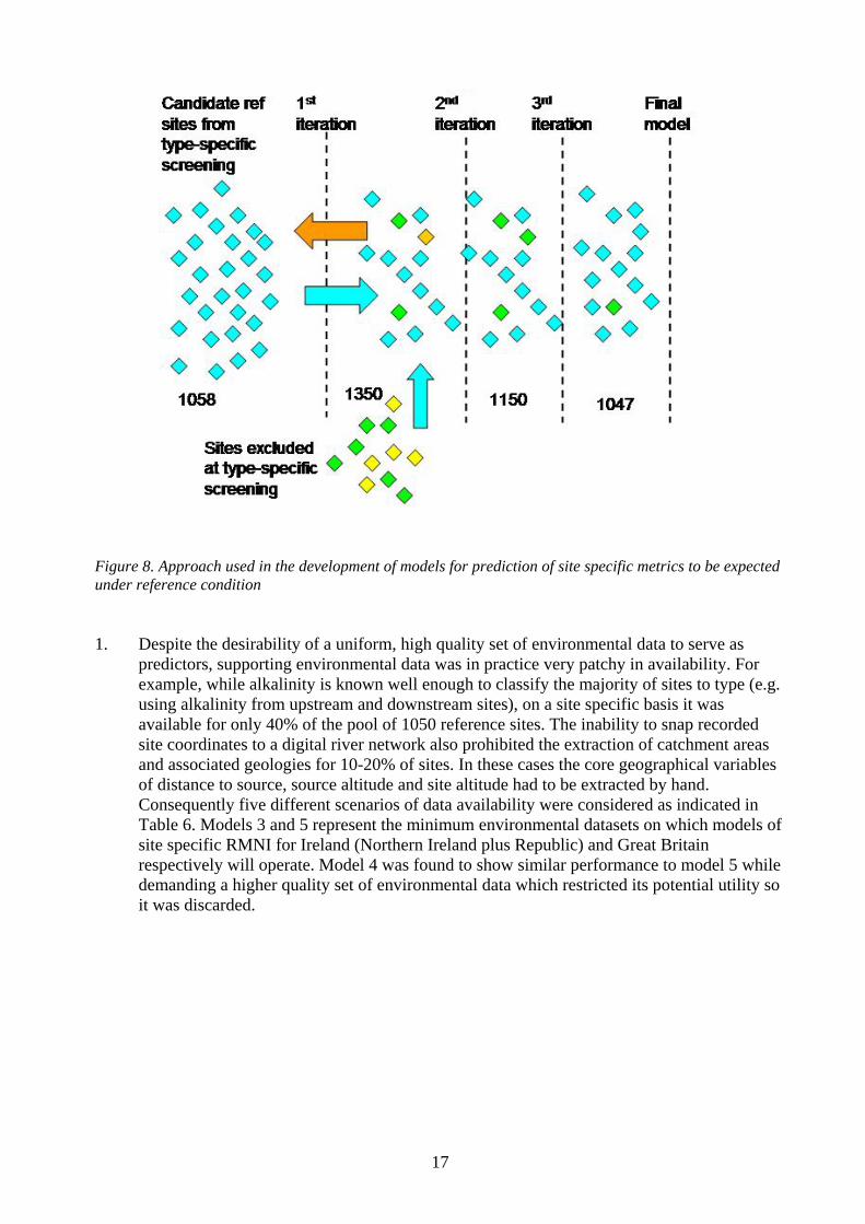
Figure 8. Approach used in the development of models for prediction of site specific metrics to be expected under reference condition 1. Despite the desirability of a uniform, high quality set of environmental data to serve as

predictors, supporting environmental data was in practice very patchy in availability. For example, while alkalinity is known well enough to classify the majority of sites to type (e.g. using alkalinity from upstream and downstream sites), on a site specific basis it was available for only 40% of the pool of 1050 reference sites. The inability to snap recorded site coordinates to a digital river network also prohibited the extraction of catchment areas and associated geologies for 10-20% of sites. In these cases the core geographical variables of distance to source, source altitude and site altitude had to be extracted by hand. Consequently five different scenarios of data availability were considered as indicated in Table 6. Models 3 and 5 represent the minimum environmental datasets on which models of site specific RMNI for Ireland (Northern Ireland plus Republic) and Great Britain respectively will operate. Model 4 was found to show similar performance to model 5 while demanding a higher quality set of environmental data which restricted its potential utility so it was discarded.

17

Table 6. Predictive variables entered in five alternative models of reference RMNI designed to accommodate variations in availability of supporting environmental data. Variables featuring in final stepwise models are shown in bold. Model 4 showed similar performance to Model 5 and was not considered further.

Input Predictors Model 1 Model 2 Model 3 Model 4 Model 5

GB Northing x X GB Easting x X Irish Northing X x Irish Easting x X Alkalinity X Slope X X X x X Distance to source X x X x X Source altitude X X X x X Site altitude X X X x X Catchment area x x Drift geology1 X x Solid geology2 x x

1. Supplied as % clay, sand, peat, rock. 2. Supplied as % calcareous or siliceous and % in four acid sensitivity classes.

The stepwise regression models obtained for models 1,2 3 and 5 are detailed in the Table 7. These models illustrate that it is possible to predict expected RMNI with a moderate to high degree of precision (± 8% of the mean for 70% of reference sites and ±11% for the remaining 30%) using a fairly minimal subset of environmental predictors.

Figure 9 . Relationship between Expected and Observed RMNI values for whole dataset with status classes overlain. The expected values are derived from the model that can predict RMNI with the lowest standard error and depend on the environmental data available for each site.

18

Table 7. Summary of stepwise regression models for predicting RMNI at reference sites based on differenscenarios of environmental data availability.

t

Model1: Alkalinity and key geographical variables knownAdjusted r2 = 0.78. Standard error of estimate = 0.41. n = 398 mean 4.83

Unstandardized Coefficients t Sig.B Std. Error

(Constant) 4.42 0.24 18.40 0.00logalk 0.92 0.04 21.11 0.00log_dist 0.56 0.07 8.43 0.00log_source_alt -0.53 0.10 -5.35 0.00log_slope -0.28 0.05 -5.54 0.00site_alt 0.00 0.00 -5.31 0.00

Model2 NI+ROI but requires catchment and associated geologyAdjusted r2 = 0.81. Standard error of estimate = 0.32. n = 207 mean 5.24

Unstandardized Coefficients t Sig.B Std. Error

(Constant) 4.54 0.29 15.91 0.00log_slope -0.63 0.05 -11.48 0.00drift Clay 0.01 0.00 11.92 0.00IrishN 0.00 0.00 3.85 0.00Height_of_Source 0.00 0.00 -3.68 0.00site_alt 0.00 0.00 -3.21 0.00

Model3 NI+ROI no alkalinity, catchment area or associated geologyAdjusted r2 = 0.68. Standard error of estimate = 0.46. n = 320 mean5.09

Unstandardized Coefficients t Sig.B Std. Error

(Constant) 4.21 0.26 15.97 0.00log_slope -0.56 0.10 -5.60 0.00IrishE 0.00 0.00 10.48 0.00Height_of_Source 0.00 0.00 -6.47 0.00site_alt 0.00 0.00 -3.20 0.00log_site_alt 0.35 0.14 2.53 0.01log_dist 0.30 0.09 3.27 0.00Slope -0.01 0.00 -2.77 0.01

Model 5 GB, no alkalinity,catchment area or associated geologyAdjusted r2 = 0.75. Standard error of estimate = 0.51. n = 727 mean 4.44

Unstandardized Coefficients t Sig.B Std. Error

(Constant) 4.02 0.12 33.26 0.00log_slope -0.45 0.05 -9.63 0.00NORTHNET 0.00 0.00 -13.08 0.00Distance_to_souce 0.00 0.00 4.60 0.00EASTNET 0.00 0.00 11.70 0.00Height_of_Source 0.00 0.00 -12.23 0.00log_dist 0.72 0.07 9.65 0.00

19

2. The main virtues of the environmental predictors in Table 7, are, that with the exception of

alkalinity, (i) all can be derived readily from maps (provided co-ordinates have been determined correctly in the field); (ii) they are spatially and temporally invariant and can be measured with minimal error; (iii) they are all genuinely un-impactable intrinsic characteristics of sites. However, some datasets also contain information on locally measured environmental variables, such as substrate, shading, depth and channel width. Although these variables cannot be used to build generally available models to be applied to existing survey data because they have been measured too infrequently, it was felt wise to check whether these variables had sufficient additional explanatory power to justify their measurement in the field in future sampling campaigns. In the assessments that were made, these local variables were highly significant when tested individually but only explained an additional 1-2% of the variation in the best models having fitted the core ‘regional’ variables. Channel width is very tightly correlated with distance from source (r2 = 0.89) and not surprisingly adds very little. Substrate is highly correlated with slope and source altitude. While it may be a more proximate influence on macrophytes than either slope or altitude there is also the risk that substrate incorporates a pressure effect through the modification of sediments via siltation.

3. To predict expected RMNI the prototype tool calculates expected RMNI using all models

for which the necessary environmental predictors are available and then selects the value that can be predicted with the lowest standard error term. Thus the choice of models is from 2>1>5>3. Figure 9 illustrates the relationship between observed and expected RMNI for 7000 river surveys with sites coloured by class assigned on the basis of EQR boundary values. The line fitted through the reference sites alone by definition represents an EQR of unity (i.e. the median reference site score).

20

9. ComComb invertsensitorganmacroother betterdiffere or Good macromacrostresse

parison with other quality elements ining the outputs of the above model with previous matches between macrophyte andebrate site data, it is possible to examine the relationship between site status based on ivity of macrophytes to nutrient enrichment and macroinvertebrates at adjacent sites to ic enrichment. The figure below illustrates that sites classified as Bad based on their phytes also typically support invertebrates with much lower mean ASPT scores than in classes (although apparently most of these sites would still be considered as being Good or for invertebrates). In the range of macrophyte class High-Moderate however, there is no nce with respect to invertebrate ASPT with the vast majority of sites classed as Highfor macrophytes being assigned High status for their macroinvertebrates. Evidently phytes show stronger differentiation over a nutrient pressure gradient than invertebrates but conditions that result in low status for macrophytes also contribute to d invertebrate faunas.

Figure 10. Relationship between final macrophyte-based class using RMNI metric (x axis) and macroinvertebrate ASPT EQR values, showing class boundaries.

21

10. Deriving regulatory standards for nutrients based on ecological status of river macrophytes Having classified sites regulatory standards can be defined by examining the relationship betweclass and the determinand considered to reflect a particular pressure. This step may add some legitimacy to the process described above in terms of boundary setting if proposed nutrientmatch current thinking for other quality elements, or hindcast values based on hisdata or inferred from diatoms.

en

values torical landuse

here are two basic options for setting regulatory values: Examine, on a type-specific basis, the distribution of values of a determinand for sites of a

given class and take an upper percentile (usually 90th) as the value corresponding to the class boundary. This is the approach currently recommended by UKTAG (2006) and is likely to perform best when sample sizes of matched biology and chemistry sites in good or high classes are very large (i.e. thousands) and there is high confidence in the spatial and temporal match between chemistry and biology data.

• Establish a continuous relationship between the metric used to classify sites and the pressure variable and use this to derive values that support High or Good Ecological Status. The attractions of this approach are its ability to fully exploit matched biology and chemistry data, to function when sample sizes are relatively small, to predict the levels of a pressure under reference condition and at the various class boundaries for any given site and, most critically, to predict the levels of a pressure at a class boundary that was defined with some ecological justification rather than defining these levels by an arbitrary percentile. Values may be considered in terms of the fitted (median) value or some percentile of the residual variation at that point, dependent on the percentage of sites in which it is considered appropriate to support that standard of ecology.

In the second case it is open to debate whether standards are more appropriately derived using a type specific relationship between the metric and pressure, or the global relationship based on all sites. The global approach is less prone to outliers and gaps at extremes of the gradient that may arise in types with a poor match to environmental data. Moreover, since many sites fall at or close to type boundaries, and because the impacted biological assemblage of one type may represent good or even reference conditions in a different higher alkalinity or lower gradient type, the global relationship approach makes use of the full dataset in deriving regulatory standards. There is a significant advantage here since most chemical monitoring has focused on impacted sites and only a minority of sites classed as high or good for macrophytes actually have contemporaneous chemica hat may aris The choice of percentiles in setting standards is critical, especially in the first approach. The use of a low percentile (e.g. 25th) would protect the biology at a high proportion of sites but equally such a standard would then be unnecessarily conservative for the majority of sites and would present considerable, and to some extent unwarranted challenges for regulators. The alternative of setting standards using an upper percentile (75th or 90th) may be preferred on the grounds that these represent the upper limits for a determinand at which biology of that class is still supported. This approach is justified (if sample sizes are large enough) while it is remembered that this standard then supports biology of that class at a minority of sites in that type and as long as the standard does not become seen as a target or an indication of the capacity of sites to absorb further pressure. The joint use of biological and physiochemical elements in site classification would ensure that sites with impacted biology at values of a pressure better than the regulatory standard would take the lower class value whereas the approach of setting a highly precautionary

T•

l data. The use of a global relationship also reduces the potential influence of outliers te as a result of weak spatial-temporal matches between datasets.

22

regulatory value carries the risk of failing sites on their physicochemistry at which the b(that was used

iology to inform those physicochemical standards) is actually relatively unimpacted.

r than an upper limit representative of the whole range of values

r High quality sites. (ii) in the case of biological and chemical monitoring that was not th invertebrate sampling) the quality of

tchtime mpercen match Value RP) and total oxidised nitrogen

with the tymatch is only applie Valuemetricfor the value for EQR=relatio

RMNIi = ((E1-E0)*EQRi)+E0

ed

t to

or

Additional problems in translating the current UKTAG approach to macrophytes are that: (i) the pool of contemporary reference sites in moderate to high alkalinity water body types almost certainly represent sites near the H/G boundary rather than core High quality sites so taking an upper percentile of available chemistry could be considered equivalent to taking an upper limit ofan already truncated range rathefospecifically linked in space and time (e.g. at GQA sites wima ing of biology to chemistry data is very variable. Filtering of paired data to an exact space-

atch drastically reduces the data on which to work and is not an option, yet an upper tile approach may be unduly influenced by outlying samples with a poorer space or time.

s are presented here for soluble reactive phosphorus (S(TON) (annual means) comparing the use of the global metric-pressure relationship method

pe specific distribution of within-class values method. Because of the limited sample sizes of ed biology and chemistry at high or good class the type-specific distribution methodd using the four group typology used by the DARES project for diatoms (Kelly et al., 2005).s can then be compared directly with those obtained for diatoms. In the case of the global -pressure relationship method, for simplicity, values have been calculated using the values median site in each class as the environmental predictors (i.e. to derive the RMNI 1). The various boundary and mid class RMNI values are then derived from the nship:

E1 is the metric value expected under reference conditions, E0 is the maximum (most degraded) metric value (in this case 9.5) EQRi is the EQR for the boundary or mid class in question (e.g. 0.78 for G/M boundary).

Each type comprises a population of sites whose intrinsic environmental characteristics range either above or below those of the median site. Members of a type will therefore have an expectRMNI score and corresponding nutrient standards for the various EQR boundaries that lie above or below those of the median site. Consequently values are also given for nutrients equivalenthe upper and lower quartiles of the distribution of expected RMNI values for the population of sites in each type. Figure 11 illustrates the global relationship between RMNI and SRP or TON that were used to derive regulatory standards. Note that RMNI is clearly the dependent variable but is used here topredict the nutrient concentrations associated with known class boundary values. These relationships were obtained after considerable screening, most notably the removal of species poor sites (4 or fewer species) at which the vegetation is often a poor indication of ambient nutrient concentrations. Sites with high or low RMNI may be linked to unexpectedly low or high nutrient concentrations respectively, perhaps because such sites were under-sampled during surveyingare recovering from disturbance (natural or anthropogenic) and represent a somewhat random sample of the potential species pool.

23

Figure 11: Global relationship between River Macrophyte Nutrient Index (x axis) and annual mean soluble

active phosphorus or Total Oxidised Nitrogen (log scale). re

y = 0.2791x + 1.5703

4

ugl-1

)

R2 = 0.594.5

0

0.5

1 2 3 4 5 6 7 8 9 10

Observed RMNI

1

1.5

2

2.5

log

TON

(

3

3.5

5

y = 0.4522eR2 = 0.5514

1.5

2

2.5

3

3.5

4lo

g SR

P (u

gl-1

)0.2177x

1

0

0.5

1 2 3 4 5 6 7 8 9 10Observed RMNI

4.5

24

Table 8. Modelled annual mean SRP values (ugl-1) at the mid points of High and Good status and H/G and G/M boundaries for the median site in each of 13 river types (bold). Upper and lower values are the concentrations associated with the 25th and 75th percentiles of expected RMNI scores for the population of sites in each river type.

DARES type LEAFPACS Type

1 LowAlk, Low Grdt 11 13 16 15 17 22 19 22 28 24 28 352 LowAlk, Mod Grdt 9 11 14 12 15 18 16 20 24 20 25 302 LowAlk, High Grdt 6 7 10 8 10 14 11 13 18 14 17 221 ModAlk, Low Grdt 18 23 29 25 31 39 32 39 50 40 49 622 ModAlk, Mod Grdt 14 17 19 19 23 26 25 29 34 31 37 422 ModAlk, High Grdt 11 13 16 14 18 21 19 23 27 24 29 343 HighAlk, Vlow Grdt 38 44 52 51 58 69 64 73 86 79 90 1053 HighAlk, Low Grdt 27 33 38 37 43 50 47 55 64 58 68 794 HighAlk, Mod Grdt 19 24 27 26 32 36 34 40 46 42 51 584 HighAlk, High Grdt 13 18 23 17 24 31 22 31 39 28 39 493 VHighAlk, Vlow Grdt 56 66 81 74 86 105 92 107 130 113 130 1573 VHighAlk, Low Grdt 39 46 54 52 61 71 65 77 89 81 95 1084 VHighAlk, Mod Grdt 24 32 38 33 42 50 42 54 63 52 67 78

High/Good mid Good Good/Modmid High

Table 9. Modelled annual mean TON values (mgl-1) at the mid points of High and Good status and H/G and G/M boundaries for the median site in each of 13 river types (bold). Upper and lower values are the concentrations associated with the 25th and 75th percentiles of expected RMNI scores for the population of sites in each river type.

DARES type LEAFPACS Type

1 LowAlk, Low Grdt 0.49 0.58 0.74 0.68 0.79 0.98 0.86 1.00 1.22 1.07 1.22 1.472 LowAlk, Mod Grdt 0.40 0.52 0.63 0.56 0.71 0.84 0.73 0.90 1.06 0.91 1.11 1.292 LowAlk, High Grdt 0.26 0.33 0.46 0.37 0.46 0.63 0.50 0.61 0.81 0.64 0.78 1.011 ModAlk, Low Grdt 0.84 1.02 1.27 1.10 1.32 1.60 1.35 1.60 1.91 1.62 1.89 2.232 ModAlk, Mod Grdt 0.66 0.78 0.89 0.88 1.02 1.16 1.10 1.27 1.42 1.34 1.53 1.692 ModAlk, High Grdt 0.49 0.60 0.73 0.67 0.82 0.97 0.86 1.03 1.20 1.06 1.25 1.453 HighAlk, Vlow Grdt 1.57 1.74 1.98 1.94 2.13 2.40 2.29 2.50 2.78 2.64 2.86 3.163 HighAlk, Low Grdt 1.20 1.39 1.57 1.52 1.73 1.94 1.83 2.06 2.29 2.14 2.39 2.634 HighAlk, Mod Grdt 0.89 1.06 1.20 1.16 1.36 1.52 1.42 1.64 1.82 1.69 1.94 2.134 HighAlk, High Grdt 0.59 0.83 1.03 0.80 1.09 1.32 1.01 1.34 1.61 1.23 1.60 1.903 VHighAlk, Vlow Grdt 2.09 2.33 2.69 2.52 2.78 3.17 2.91 3.19 3.60 3.30 3.59 4.013 VHighAlk, Low Grdt 1.60 1.81 2.02 1.97 2.22 2.45 2.32 2.59 2.84 2.67 2.96 3.224 VHighAlk, Mod Grdt 1.09 1.36 1.56 1.40 1.70 1.93 1.69 2.03 2.27 1.99 2.36 2.62

mid High High/Good mid Good Good/Mod

25

The tabulated values (Tables 8and 9) are derived from the fitted lines using the median, 25th and 75th percentiles of the distribution of expected RMNI scores for each river type (i.e. EQR = 1) anthe equivalent RMNI scores associated with H/G, mid Good and G/M EQR equivalents of 0.90.84 and 0.78 respectively. Values calculated by this

d 1,

approach are typically about twice as high at /M boundary as at the mid-point of High and the upper and lower values for a boundary or class

mid-point are typically ± 10-20% of the median. 10.1 Comparison with standards proposed by UKTAG based on diatoms By aggregating macrophyte survey data in line with the four group typology employed by the DARES project Table 10 provides a direct comparison with the standards proposed by UKTAG based on diatoms. Relative to the macrophyte dataset the diatom –chemistry dataset is a high quality match of sampling in space and time for sites of high or good status. In the case of macrophytes, the application of the upper percentile approach to small sample sizes produces inconsistent trends between High and Good status due to the influence of outliers, although this is improved by the use of the 75th percentile. While diatoms are certainly more responsive than macrophytes to short term increases in nutrient loading there is little evidence that they are more sensitive to prolonged exposure to increased nutrient loads. Generally, comparisons here between standards suggested by diatoms and

acrophytes are probably therefore distorted more by differential quality of data than indicative f differences in sensitivity of these quality elements. The global relationship approach is onsidered to offer a far superior guide to the setting of standards for macrophytes and it would be aluable to assess the effect of applying this approach to diatoms. This approach applied to acrophytes generally compares very favourably to the standards established for diatoms based

able 10. Comparison of the upper percentile, type specific approach to derivation of SRP standards (annual mean ugl-1) for macrophytes with values derived for diatoms and with the use of the global-relationship approach, using the DARES four group typology as a reporting framework.

G

mocvmon the selection of upper percentile values for a class on type-specific basis but suggests the need for rather more conservative standards in the higher altitude stream types (2 and 4), especially at the G/M boundary. T

GOODDARES River Type

n 90th 75th modelled H/G Diatoms n 90th 75th modelled G/M DiatomsLow alk, low alt (1) 121 96 60 27 30 119 312 80 44 50Low alk, high alt (2) 115 51 27 16 20 84 58 50 27 40High alk, low alt (3) 81 493 98 63 110 407 243 97High alk, high alt (4) 49 90 26 32 56 110 85 51

120

macrophytesHIGH

macrophytes

50

0.2 Comparison with other standards he values that emerge for macrophytes using the global-relationship approach are generally losely convergent with WFD characterisation work and Habitats Directive standards (Pitt et al., 002) as reviewed in the UK Environmental Standards report (UKTAG, 2006). For example, the roposed guideline standard for SRP of 60ugl-1 for chalk stream SACs that might be aligned with

1Tc2p

26

the middle of Good status agrees well with values of 77 and 54 (types 12 and 13) in the current analysis. The threshold value for chalk streams of 100ugl-1 SRP, that could be considered as near the mid point of Moderate status, is compatible with values of 95 and 67ugl-1 SRP proposed as thG/M boundary for this river type in the present analysis. The main area of departure from the Habitats Directive s

e

tandards is in the case of natural values r rivers on calcareous geologies (suggested standard 20-30 ugl-1 compared with 45 ugl-1 (range

0-55 ugl-1) as the mid-point of High for low altitude, base-rich rivers (DARES Type 3) in the ms of guideline and

e

cy d an

in lowland base-rich rivers may be more akin to a ear total absence of any human impact which maybe incompatible with the pre-Industrial 1800-

on 0 ugl-1

owland

allow,

it is commonly assumed that production in freshwaters is phosphorus limited is assumption may not hold in lowland lakes or rivers that are well supplied with phosphorus

nd in which nitrogen is likely to be relatively mobile. The standards suggested by the present ) are

d storical

xport coefficient models which suggest nitrate concentrations of c 2mgl in the early 900s.

10.3 Causation and association Demonstrating a correlation between community composition, or a community-based metric, such as RMNI, and nutrient concentrations does not prove that macrophytes respond directly to nutrients per se (or specifically their annual average concentrations). While it is widely recognized that there is a general ecological response to a suite of specific physicochemical and biological changes that occur under the general banner of nutrient enrichment, most of the field-based ‘evidence’ for a direct effect of nutrients on macrophytes is tenuous given the problem of multiple highly intercorrelated factors. Variance partitioning methods that attempt to deal with

is problem by identifying unique and shared effects of different variables simply risk throwing e baby out with the bath water. Experimental manipulation of nutrient supply under controlled

rovide some of the most convincing evidence for a cause-rm,

fo4present analysis). This is more surprising given the close agreement in terthreshold standards for all river types and natural standards for siliceous rivers, coupled with thfact that reference conditions for macrophytes in base-rich rivers were pre-validated against thosefrom base-moderate/poor rivers to reduce the risk of including degraded sites. Some discrepanis to be expected since the Habitats Directive standards were based on expert judgement anassessment of the risk to all features of interest in riverine SACs, not just macrophytes. The Habitats Directive standards for ‘natural’ envisages an absence of significant human pressure. However, concentrations of 20-30ug l-1 SRPn1850 baseline that was used when identifying WFD reference condition sites for macrophytes. Sources including historical measurements, borehole data and export coefficient models based historical landuse data and livestock densities are compatible with values in the range 30-5SRP in lowland base-rich rivers during the nineteenth century. There may also be an additional issue of reduced sensitivity of macrophytes to nutrient enrichment in some larger, deeper, lrivers if a combination of depth, shade or turbidity, fine substrate, and grazing or scouring of epiphytes by flow leads to reduced interaction with filamentous algae compared to small, shsiliceous systems. The approach used also generates a set of standards for TON which have not been previously available. Although thaanalysis (0.5-2.8 mgl-1 and 0.8-3.6 mgl-1 TON at the H/G and G/M boundaries respectivelythus broadly in line with the suggested need for tighter controls on nitrate loading to achieve GooEcological status. For lowland rivers the values predicted for High status are in line with hirecords and e -1

1

ththconditions, for example in mesocosms, peffect relationship between nutrients and macrophytes, but such studies are invariably short temay lack realism, and may still fail to identify the true basis of the ecological response.

27

Even when only a weak effect of nutrients is found in the field this may arise because the wrongaspect (e.g. average nutrient concentration) of a pressure (e.g. eutrophication) has been chosen to reflect that pressure, not because the quality element is insensitive to the pressure as a whole. Other measures, such as nutrient loading, landuse, siltation

, sediment oxygen supply, haracteristics of the nutrient supply regime, particular nutrient fractions, or sediment as opposed

r

Volume 2 Technical Annex. ITE/DETR

d

rfield, I. (1992) A botanical classification of standing waters in

,

cto waterborne concentrations may prove better indicators of a pressure as perceived by a particulabiological quality element but such information is more difficult to obtain. It is simply convenient to use routinely monitored determinands as a marker for a pressure that needs to be managed rather than inferring anything about the precise mode of effect. Thus the most appropriate Program of Measures is that which manages a pressure to the extent that the physicochemical environment is restored to a level at which biology of a particular status is supported; this requires the use of simply measured determinands both to set a target and gauge the performance of a POM, even if that determinand per se is not the exact aspect of a pressure to which the biology responds. References Davidson, T.A., Sayer, C.D., Bennion, H., Rose, N., David, C., & Wade, M. (2005). A 250 year comparison of historical, macrofossil and pollen records of aquatic plants in a shallow lake. Freshwater Biology 50: 1671-1686 Hill, MO, Mountford, JO, Roy, DB & Bunce RGH (1999) Ellenberg’s indicator values for British plants. ECOFACT Hill, MO, Mountford, JO, Roy, DB & Bunce RGH (2000) Extending Ellenberg’s indicator values to a new area: an algorithmic approach. J. Appl. Ecol 37: 3-15. Holmes, NTH, Boon, P. & Rowell, T. (1999) Vegetation communities of British rivers: a reviseclassification. JNCC, Peterborough.

Kelly, M., Juggins, S., Guthrie, R. & Jamieson, J. (2005). Nutrient and acid conditions required to support good ecological status in benthic diatom assemblages in rivers. RTT56.

Palmer, M.A., Bell, S.L. & ButteBritain: applications for conservation and monitoring. Aquatic Conservation: Marine and freshwater ecosystems 2: 125-143

Pitt, J, Phillips, G & Mainstone, C (2002) The application of phosphorus standards to SAC riversDraft technical guidance note. UKTAG (2006) UK Environmental Standards and conditions (Phase 1) UK Technical AdvisoryGroup on the Water Framework Directive.

28

Appendix 1

Calculating species ranks for a perceived pressure from a global dataset using a draft expertranking system 1. Take a site x species dataset. The sites should be widely distributed geographically,

should represent a randomized sample of the resource, and not be biased towards particular areas or lake or river types (unless these are naturally water body rich). Multipsurveys of single water bodies should be averaged if necessary. Data can be cover von a standard scale or can be expressed as presence-absence. If large amounts of data frdifferent sources and obtained by different methods are being pooled then analyzing presence-absence data is likely to be more robust.

2. For

le alues

om

each site calculate a site index score using an available expert ranking system, by calculating the average cover-weighted rank of the species present. The Ellenberg system, which includes a fertility rank, provides the most comprehensive set of rankings for European plant species and has been adapted for the British flora as part of the ECOFACT project (Hill et al., 1999). The MTR or TRS systems for rivers and lakes respectively

also be used, or some hybrid of these systems. If species are present that do not have

. Take the species x sites dataset and the site index scores and perform a DCCA with the site

. Take the original expert ranks and regress these against the DCCA axis 1 species scores.

ed rank scaled according to the original ranking system (NB: this step can also be employed during intercalibration if the

.

full set of site index scores as the independent variable. Once rescaled to match the direction and scale of

hown d see if this can be readily explained. Under such

circumstances there is a risk that the adjusted expert score for rare species (<10

re misrepresentative of its ecological niche rather than because the (indeed many rare species have been the specific focus of detailed

herefore suggested that a global regression of original versus adjusted expert ranks using only those species with >10 occurrences is used instead to generate a new score.

6. Calculate a site index score using the adjusted values, possibly incorporating the (final DCCA derived) tolerance as a measure of the indicator potential of different species.

coulda rank ensure that the calculation of the site index is based only on the cover of ranked species.

3

index scores as the ‘environmental’ variable. 4

For species with no rank in the original system apply the regression equation to the DCCA1 axis score of that species in order to obtain a fitt

inclusion of data from other countries within a GIG introduces species that were absent from the British site database)

5. Repeat steps 2 and 3 until all species have a rank and a site index score is available for all sites. Usually only 2 iterations are required. Then carry out a DCCA with

the original system the axis 1 scores and associated tolerance values produced by this analysis form the new “adjusted expert scores”. It is useful at this stage to assess the relationship between the original and adjusted scores to identify species that have sthe largest change in rank an

occurrences) is wrong because that species is under-sampled and the sites (or vegetation) where it was recorded aexpert view is incorrectautecological studies). When species are rare in the dataset and show a marked departure from their original expert score it is t

29

7. This approach is described in detail in Hill et al. (2000). The details given above differ very slightly and do not require the use of specific software but the mechanics of the approach and results are effectively the same (Mark Hill, pers comm.)

30

1

Case: BE-FL Status: input for intercalibration exercise For further details see Schneiders et al. (2004), Leyssen et al. (2005). Internet source: http://www.instnat.be/content/page.asp?pid=PUB_Rapporten. Indicators Macrophyte taxonomic composition Species composition covers all charophytes, some non-charophyte algae (undifferentiated filamentous algae, Batrachospermum, Enteromorpha, Hydrodyction) and all angiosperms classified as hydrophyte or phreatophyte, as well as selected aphreatophytes, mosses and liverworts; ‘sewage fungus’ is also considered. All taxa included in the assessment are listed in Annex 1 (this list is updated regularly for taxa newly recorded in rivers). Thirteen growth forms are distinguished: lemnid, ricciellid, large pleustophyte (incl. stratiotid, hydrocharitid), ceratophyllid, charid, magnopotamid, batrachid and peplid (incl. Callitriche), other rooting caulescent hydrophyte (incl. parvopotamid, myriophyllid and elodeid), nymphaeid, vallisnerid, small and medium-sized helophyte, large monocotyledonous helophyte and aquatic mosses. Macrophyte abundance The abundance of macrophyte taxa is scored on the scale shown in Table 1. Site characteristics, structure of aquatic vegetation, occurrence of growth forms and abundance of submerged plants (cf. infra) are also recorded. Table 1. Macrophyte abundance scale used for rivers. score abundance criteria weight 1 rare less than 3 plants 1 2 occasional > 3 plants, insignificant cover 1 3 frequent large number of plants, cover < 5 % 2 4 sub-abundant cover 5-25 % 3 5 abundant cover 25-50 % 4 6 co-dominant cover 50-75 % 5 7 dominant cover 75-100 % 6 Additionally, the total abundance of submerged vegetation is estimated for smaller river types as in Table 2. Table 2. Assessment of aquatic vegetation abundance for smaller river types.

abundance submerged vegetation score average score stretch EQR 0 absent 0 1.6-2 0.8-1 1 scarce 1 1.2-<1.6 0.6-<0.8 2 (fairly) abundant but not filling the water column 2 0.8-<1.2 0.4-<0.6 3 filling the entire water column 1 0.4-<0.8 0.2-<0.4 0-<0.4 0-<0.2

Bacterial tufts Presence and abundance of sewage fungus is considered. Summary Four metrics in the form of EQRs (scaled 0-1), covering both structural and functional aspects of the aquatic vegetation, are used to assess ecological status in terms of species composition and abundance:

relative abundance of type-specific taxa, relative abundance of disturbance indicators, diversity of growth forms, and, for some smaller river types only, abundance of submerged vegetation.

The standard list specifies how taxa are classified to calculate the metrics for type specificity and disturbance (Leyssen et al. 2005, Annex 1). All the metrics are considered equally important and are combined by taking the lowest value for any one of them as the final EQR (‘one out, all out’). Macrophyte assessment is not constrained by requiring the presence of a minimum number of species or an abundance treshold. Macrophytes and phytobenthos are

2

assessed independently of each other as different quality elements and considered on an equal basis using the ‘one out, all out’ principle. Monitoring Strategy Several 100 m stretches are considered to assess the status of an entire water body (WB). At least 3 stretches are surveyed per WB, each one positioned randomly within the upstream, midstream and downstream part, respectively (division into parts based on equal length or stream confluence). The exact location of each stretch is adapted in accordance to local conditions (accessibility, lack of dense shading,…) to within 1 km or 500 m (depending on WB type) up- or downstream of the initial random point. If this proves impossible, another random location is determined as a starting point. Relevés are made of the stream bed vegetation along 100 m river stretches and, if necessary, from both banks. Overall light and substrate conditions along these stretches should allow unhindered plant growth. Vegetation is surveyed by wading upstream through the water, from a boat and/or from the shore, whatever is most appropriate or feasible. Abundance and growth form are noted for individual taxa. Optionally, relevés can be made of the stream bank vegetation, including both left and right side of the selected stretches, up to the normal winter water level. When, frequency? Once a year. Preferably in summer (mid June to August), possibly extending into early Autumn for certain sites. Depending on the vegetation composition or observed phenology, an additional visit may be made in spring (May) or early summer to allow complementary observations. Equipment A 50 cm broad mesh-covered rake on a telescopic handle (up to 4 m long) or a similar double-sided rake fixed to a 20 m rope are used to collect plants where necessary. Plastic bags and jars to hold collected specimens. Binoculars, magnifying glasses (10x, 20x). Analysis Identification is done in the field, if possible, using appropriate keys. If necessary, this is validated or completed in the laboratory. In case identification proves impossible due to lack of certain parts at the time of survey, additional visits to the site are made in a more appropriate season. Voucher material is retained, dried or in a preserving liquid, of difficult or dubious specimens. Angiosperms, charophytes, mosses and liverworts are identified to species level. Some non-charophyte algae are considered at genus level; sewage fungus and filamentous algae are recognized by general aspect, only. Reporting No procedures have been established, yet. Assessment Data requirements Attribution of the WB to a water type. Macrophyte survey data for individual stretches. Calculation The EQR for type-specific species composition (TS) indicates the relative abundance-weighted agreement between the observed species composition and that expected for the water type. For each water type, specificity values are attributed to individual species in the standard list (0: species does not occur naturally; 1: occurrence possible in natural conditions; Annex 1). Most type-specific taxa can occur in several types. The notion of ‘type specificity’ (in the sense of naturalness) also depends strongly on the perception of neophytes. Aggressive non-native species (marked with Z in Annex 1) are not considered type specific in the calculation of TS, although Annex 1 indicates the types in which they usually occur. The treatment of other neophytes may be reconsidered in the future. The EQR is calculated by means of the formula:

3

TS = ( )

∑

∑

=

=

⋅

n

ii

n

iii

Ab

tsAb

1

1

Abi : abundance of taxon i; tsi : type-specificity value of taxon i (0 or 1); n : number of observed taxa included in the standard list; TS : index for type specificity.

The EQR for the abundance of disturbance indicators (V) gives the relative abundance-weighted representation of pollution (sewage, eutrophication, acidification,…) indicative species. These are taxa assumed to increase in abundance with increasing chemical pressures. Only the most reliable disturbance indicators are selected for each water type (0: no marked indication; 1: deteriorating quality with increasing abundance). Note that type-specific taxa can be disturbance indicators. The index is calculated as:

V = 1 - ( )

∑

∑

=

=

⋅

n

ii

n

iii

Ab

vAb

1

1

Abi : abundance of taxon i; vi : perturbation value of taxon i (0 or 1); n : number of observed taxa included in the standard list; V : index for disturbance.

The abundance classes are weighted as indicated in Table 1. For the calculation of the indices TS and V, the abundance classes ‘rare’ (1) and ‘occasional’ (2) are merged and weighted as 1. For each water type, an expected spectrum and diversity of macrophyte growth forms is specified for the aquatic vegetation (= only the vegetation in the water at the time of surveying) to enable the calculation of a corresponding relative metric (GV). Expectations envisage a functionally ‘complete’ system with normal vegetation development. Only the presence of growth forms, not their abundance, is taken into account in view of the variation that may occur within a water type at the relevé scale under natural conditions. Growth forms observed in the field are scored according to Table 3 and the sum obtained is used to calculate an EQR using the key given in Table 4 and linear interpolation. Presence of growth forms other than those listed in the table is not taken into account. If taxa indicating an exceptional ecological quality are present (specified by B in Annex 1), their number is added to the observed sum1. Table 3. Scoring of macrophyte growth forms for regional river types (bkK small brook Kempen, bgK large brook Kempen, bk small brook, bg large brook, rk small river, rg large river, rzg very large river; not shown for headwaters and polder ditches). Flemish type bkK bgK bk bg rk rg rzg GIG type RC-1 RC1/RC-4 RC-1 RC1/RC-4 RC-4 RC-4/R-C5 - lemnid - 1 - 1 1 1 1 ricciellid - 1 - 1 1 1 - large pleustophyte 1 1 - - - - - ceratophyllid - 1 - 1 1 1 1 charopyte 1 1 1 1 - - 1 rooting caulescent hydrophyte p.p. 1 1 1 1 1 1 1 magnopotamid 1 1 1 1 1 1 1 nymphaeid 1 1 1 1 1 1 1 batrachid and peplid (incl. most Callitriche) 1 1 1 1 - - 1 vallisnerid 1 1 1 1 1 1 1 aquatic moss, incl. sphagna 1 - 1 - - - - small and medium-sized helophyte 1 1 1 1 1 1 1 large monocotyledonous helophyte 1 1 1 1 1 1 1 For the smaller water types, bkK, bk, bgK and bg, both a reduced abundance as well as an excessive development of aquatic vegetation are considered to indicate human impact. This is expressed by the EQR for vegetation abundance (VO). In each stretch, the abundance of submerged vegetation is estimated for ten 10 m sections on a scale from 0 to 3 (Table 5). The averaged score for the 100 m stretch is converted by means of Table 5 and linear interpolation.

1 The alternative to use such species for differentiating between good and high status will be examined further.

4

Table 4. Translation of the number of growth forms to an EQR for the regional river types (cf. Table 3). Flemish type bkK bgK bk bg rk rg rzg GV range and corresponding status class RC-1 RC1/RC-4 RC-1 RC1/RC-4 RC-4 RC-4/R-C5 -

high: 0.8 - 1.0 7 - 10 (>10=10)

9 -12 (>12=12)

7 - 9 (>9=9)

6 - 11 (>11=11)

7 - 9 (>9=9)

7 - 9 (>9=9)

7 - 10 (>10=10)

good: 0.6 - <0.8 5 - 6 6 - 8 5 - 6 4 - 5 5 - 6 5 - 6 5 moderate: 0.4 - <0.6 3 - 4 4 - 5 3 - 4 2 - 3 4 4 3 poor: 0.2 - <0.4 2 2 - 3 2 1 2 - 3 2 - 3 2 bad: 0 - <0.2 0 - 1 0 - 1 0 - 1 0 0 - 1 0 - 1 0 Table 5. Assessment of aquatic vegetation abundance for smaller river types.

abundance submerged vegetation score average score stretch VO status 0 absent 0 1.6-2 0.8-1 high 1 scarce 1 1.2-<1.6 0.6-<0.8 good 2 (fairly) abundant but not filling the water column 2 0.8-<1.2 0.4-<0.6 moderate 3 filling the entire water column 1 0.4-<0.8 0.2-<0.4 poor 0-<0.4 0-<0.2 bad

For the optional relevés of the bank vegetation, separate TS and V values can be calculated as indicated above using Annex 1. These metrics may be included in the assessment as additional EQRs. Pending further investigation, however, the metrics for bank vegetation will not be considered in status classification for the WFD at present. Final EQR The final quality score (EQR) for a stretch is determined by the status of the 3 or 4 EQRs for the stream bed vegetation (optionally 5 or 6 in case bank vegetation is included) and reported as the lowest score of all metrics. General guidelines for applying the method to artificial and heavily modified water bodies are given by Leyssen et al. (2006; cf. link in Introduction). The EQR scale is divided into five equal classes for all metrics to indicate status class (Table 6). Table 6. EQR values in relation to classification.

class EQR = minimum(TSw, TSo, Vw, Vo , GV, VO) high 0.80 – 1 good 0.60 – <0.80 moderate 0.40 – <0.60 poor 0.20 – <0.40 bad 0 – <0.20

Example Site descriptors:

• regional type: small brook Kempen (bkK); • vegetation data: see colums abundance and species in Table 7.

Index 1 - TS: type-specific species composition (see colums ‘ts’ and ‘ts*weight’ in Table 7):

84.01323111

11131213111111=

+++++++⋅+⋅+⋅++⋅+⋅+⋅+⋅

=K

KTS (high)

Index 2 - V: abundance of disturbance indicators (see colums ‘v’ and ‘v*weight’ in Table 7):

43.01323111

111312130111011 =+++++++

⋅+⋅+⋅++⋅+⋅+⋅+⋅−=

K

KV (moderate)

Index 3 - GV: growth forms (Table 8):

• growth forms present are: sum = 7 (the growth forms ‘filamentous algae’ and ‘lemnid’ are not relevant for this river type, see Table 3);

• no species indicates exceptional quality (Annex 1, B): sum = 7 + 0 = 7;

5

• EQR GV = 0.8 (high; Table 4). Table 7. Example data of a 100 m stretch and calculation of TS and V. species abundance weight ts ts*weight v v*weight Alisma plantago-aquatica 1 1 1 1 0 0 Bidens tripartita 1 1 1 1 1 1 Callitriche hamulata 2 1 1 1 0 0 Callitriche obutsangula 4 3 1 3 1 3 filamentous algae 3 2 0 0 1 2 Elodea canadensis 3 2 1 2 0 0 Iris pseudacorus 1 1 1 1 0 0 Lemna minor 2 1 1 1 1 1 Lemna minuta 2 1 0 0 1 1 Mentha aquatica 2 1 1 1 0 0 Myosotis scorpioides 2 1 1 1 0 0 Myriophyllum spicatum 2 1 1 1 1 1 Nasturtium officinale 3 2 1 2 0 0 Polygonum hydropiper 1 1 1 1 0 0 Potamogeton crispus 3 2 1 2 1 2 Potamogeton natans 3 2 1 2 0 0 Potamogeton perfoliatus 4 3 1 3 0 0 Potamogeton trichoides 4 3 0 0 1 3 Ranunculus sceleratus 1 1 1 1 1 1 Rumex hydrolapathum 2 1 1 1 0 0 Sagittaria sagittifolia 3 2 1 2 1 2 Sparganium emersum 4 3 1 3 1 3 Sparganium erectum 1 1 1 1 1 1 sum 37 31 21 EQR TS 0.84 V 0.43

Table 8. Calculation of the index growth forms (GV). growth form species scorefilamentous algae filamentous algae 0

Lemna minor lemnid Lemna minuta

0

parvopotamid* Potamogeton trichoides myriophyllid* Myriophyllum spicatum elodeid* Elodea canadensis

1

Potamogeton crispus magnopotamid Potamogeton perfoliatus

1

nymphaeid Potamogeton natans 1Callitriche hamulata peplid Callitriche obutsangula

1

Sagittaria sagittifolia vallisnerid Sparganium emersum

1

Alisma plantago-aquatica Bidens tripartita Mentha aquatica Myosotis scorpioides Nasturtium officinale Polygonum hydropiper Ranunculus sceleratus

small and medium-sized helophyte

Rumex hydrolapathum

1

Iris pseudacorus large monocotyledonous helophyte Sparganium erectum

1

number of growth forms 7EQR GV 0.8

* rooting caulescent hydrophytes Index 4 - VO: vegetation abundance (Table 9):

• average score over 100 m: 1.3;

6

• VO = 1.3/2 = 0.65 (good). Table 9. Calculation of index vegetation abundance (VO). stretch submerged abundance score 0 – 10 m 2 2 10 – 20 m 2 2 20 – 30 m 3 1 30 – 40 m 3 1 40 – 50 m 3 1 50 – 60 m 1 1 60 – 70 m 2 2 70 – 80 m 1 1 80 – 90 m 1 1 90 – 100 m 1 1

average score over 100 m 1.3 EQR 0.65

Final EQR: MIN(0.84, 0.43, 0.8, 0.65) = 0.43 (moderate; due to V). The mathematical integration of multiple EQRs for stretches into a single EQR for a water body, for instance as the lowest or (weighted) average value, has not yet been decided. Reference, H/G, G/M Contemporary references are absent or extremely scarce for all types prohibiting a spatial reference approach. The assessment is therefore based on vegetation attributes which can be estimated from the remaining sites presenting higher quality, historical records, and information on the behaviour of individual species and the structural response of aquatic vegetations in relation to pressures, making as few assumptions as possible. This information is integrated by expert judgement. Expectations for growth form diversity are based mainly on expert judgement, envisaging a functionally ‘complete’ system with undisturbed vegetation succession for each water type. Development of submerged vegetation is added as a robust semi-quantitative assessment of the expected response in productivity to eutrophication, mainly, with both reduced and superfluous abundance leading to a lower status assessment. Boundary values are set mainly by expert judgement with the requirement that good status can only be attained if taxa which are not specific for the water type or indicate disturbance remain notably less abundant relative to type-specific and non-disturbance species. These boundaries may be revised in the harmonisation process and as more information from monitoring becomes available. The corresponding EQR scale is divided into equal classes, which will not require revision, as such. Correlation to pressures The EQR is designed to reflect the combined effect of hydrochemical, hydromorphological and biological pressures in terms of deviation from reference characteristics and functional impairment for the purpose of general status and trend monitoring (operational monitoring may involve only particular metrics or different methods). Consequently, lower values are expected from a significant increase in any potential pressure. As the individual metrics respond to different pressures, the combined EQR will only show a clear response to a single selected pressure, such as eutrophication, in the absence of any other pressures. Site selection in the intercalibration only considers possible impact by eutrophication, however. Moreover, most methods considered in the intercalibration are designed to track (only) this specific pressure, reducing their comparability to the BE-FL-approach. The different metrics will respond respectively, most strongly to:

• TS: overall hydrochemical alteration, sediment quality, invasive species; • V: eutrophication, pollution; • GV: eutrophication, pollution, sedimentation/erosion, dredging, weed cutting; • VO: eutrophication, pollution (incl. thermal pollution), hydromorphological change,

dredging, weed cutting. Table 10 (next page). Spearman rank correlation matrix of metrics and water quality variables for all available surveys in bkK and bgK streams. Significant values (p ≤ 0.05) are in yellow.

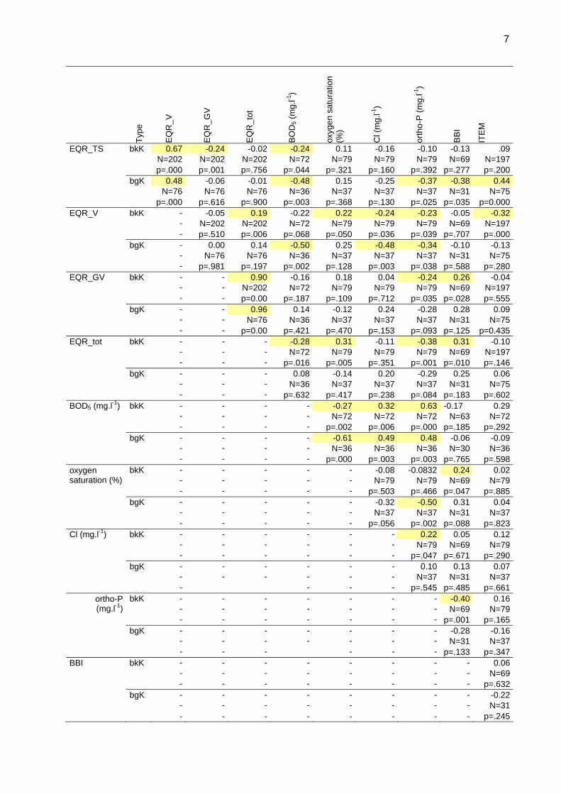
7

Type

EQ

R_V

EQ

R_G

V

EQ

R_t

ot

BO

D5 (

mg.

l-1)

oxyg

en s

atur

atio

n

(%)

Cl (

mg.

l-1)

orth

o-P

(mg.

l-1)

BB

I

ITE

M

EQR_TS bkK 0.67 -0.24 -0.02 -0.24 0.11 -0.16 -0.10 -0.13 .09 N=202 N=202 N=202 N=72 N=79 N=79 N=79 N=69 N=197 p=.000 p=.001 p=.756 p=.044 p=.321 p=.160 p=.392 p=.277 p=.200 bgK 0.48 -0.06 -0.01 -0.48 0.15 -0.25 -0.37 -0.38 0.44 N=76 N=76 N=76 N=36 N=37 N=37 N=37 N=31 N=75 p=.000 p=.616 p=.900 p=.003 p=.368 p=.130 p=.025 p=.035 p=0.000EQR_V bkK - -0.05 0.19 -0.22 0.22 -0.24 -0.23 -0.05 -0.32 - N=202 N=202 N=72 N=79 N=79 N=79 N=69 N=197 - p=.510 p=.006 p=.068 p=.050 p=.036 p=.039 p=.707 p=.000 bgK - 0.00 0.14 -0.50 0.25 -0.48 -0.34 -0.10 -0.13 - N=76 N=76 N=36 N=37 N=37 N=37 N=31 N=75 - p=.981 p=.197 p=.002 p=.128 p=.003 p=.038 p=.588 p=.280EQR_GV bkK - - 0.90 -0.16 0.18 0.04 -0.24 0.26 -0.04 - - N=202 N=72 N=79 N=79 N=79 N=69 N=197 - - p=0.00 p=.187 p=.109 p=.712 p=.035 p=.028 p=.555 bgK - - 0.96 0.14 -0.12 0.24 -0.28 0.28 0.09 - - N=76 N=36 N=37 N=37 N=37 N=31 N=75 - - p=0.00 p=.421 p=.470 p=.153 p=.093 p=.125 p=0.435EQR_tot bkK - - - -0.28 0.31 -0.11 -0.38 0.31 -0.10 - - - N=72 N=79 N=79 N=79 N=69 N=197 - - - p=.016 p=.005 p=.351 p=.001 p=.010 p=.146 bgK - - - 0.08 -0.14 0.20 -0.29 0.25 0.06 - - - N=36 N=37 N=37 N=37 N=31 N=75 - - - p=.632 p=.417 p=.238 p=.084 p=.183 p=.602BOD5 (mg.l-1) bkK - - - - -0.27 0.32 0.63 -0.17 0.29 - - - - N=72 N=72 N=72 N=63 N=72 - - - - p=.002 p=.006 p=.000 p=.185 p=.292 bgK - - - - -0.61 0.49 0.48 -0.06 -0.09 - - - - N=36 N=36 N=36 N=30 N=36 - - - - p=.000 p=.003 p=.003 p=.765 p=.598

bkK - - - - - -0.08 -0.0832 0.24 0.02oxygen saturation (%) - - - - - N=79 N=79 N=69 N=79 - - - - - p=.503 p=.466 p=.047 p=.885 bgK - - - - - -0.32 -0.50 0.31 0.04 - - - - - N=37 N=37 N=31 N=37 - - - - - p=.056 p=.002 p=.088 p=.823Cl (mg.l-1) bkK - - - - - - 0.22 0.05 0.12 - - - - - - N=79 N=69 N=79 - - - - - - p=.047 p=.671 p=.290 bgK - - - - - - 0.10 0.13 0.07 - - - - - - N=37 N=31 N=37 - - - - p=.545 p=.485 p=.661

bkK - - - - - - - -0.40 0.16ortho-P (mg.l-1) - - - - - - - N=69 N=79

- - - - - - - p=.001 p=.165 bgK - - - - - - - -0.28 -0.16 - - - - - - - N=31 N=37 - - - - - - p=.133 p=.347BBI bkK - - - - - - - - 0.06 - - - - - - - - N=69 - - - - - - - - p=.632 bgK - - - - - - - - -0.22 - - - - - - - - N=31 - - - - - - - - p=.245

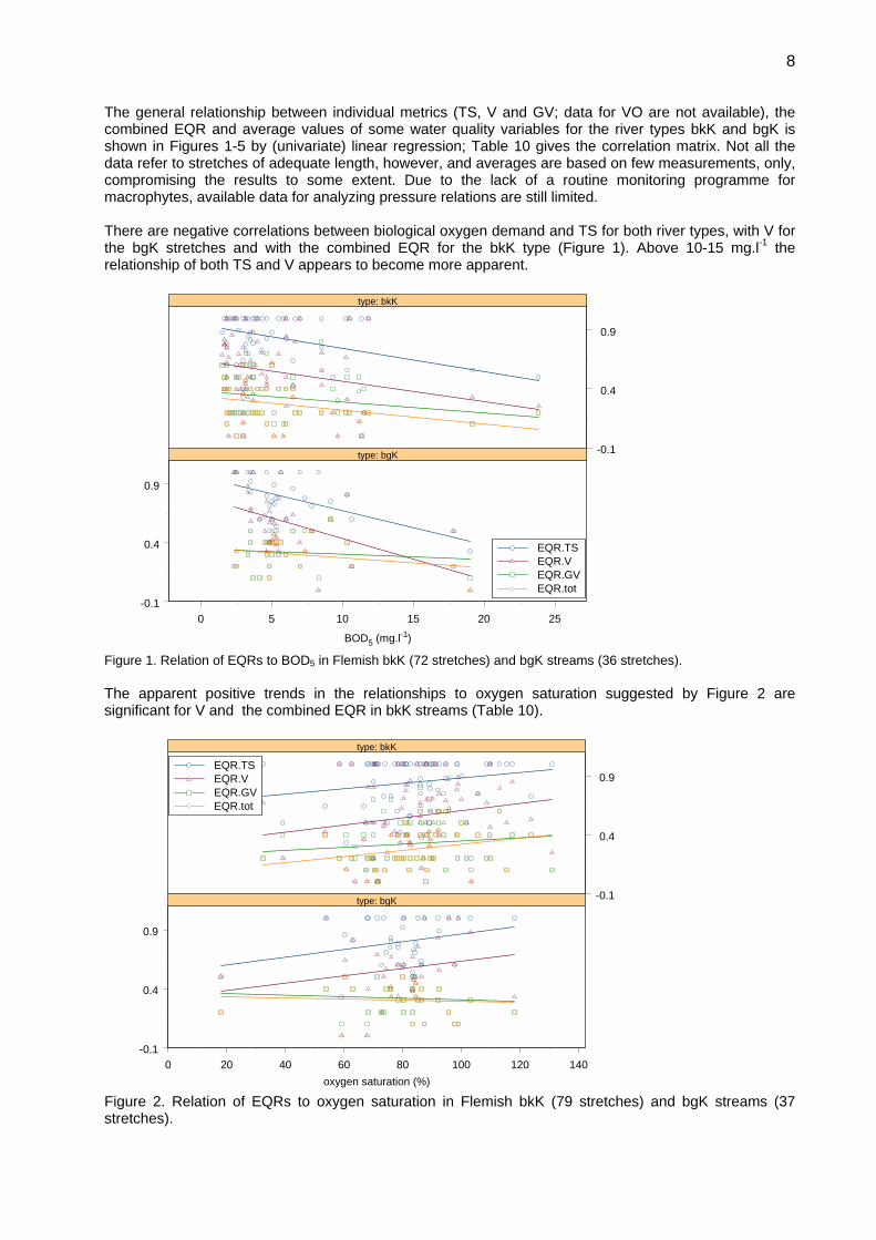
8

The general relationship between individual metrics (TS, V and GV; data for VO are not available), the combined EQR and average values of some water quality variables for the river types bkK and bgK is shown in Figures 1-5 by (univariate) linear regression; Table 10 gives the correlation matrix. Not all the data refer to stretches of adequate length, however, and averages are based on few measurements, only, compromising the results to some extent. Due to the lack of a routine monitoring programme for macrophytes, available data for analyzing pressure relations are still limited. There are negative correlations between biological oxygen demand and TS for both river types, with V for the bgK stretches and with the combined EQR for the bkK type (Figure 1). Above 10-15 mg.l-1 the relationship of both TS and V appears to become more apparent.

0 5 10 15 20 25

BOD5 (mg.l-1)

-0.1

0.4

0.9

-0.1

0.4

0.9

type: bgK

type: bkK

EQR.TSEQR.VEQR.GVEQR.tot

Figure 1. Relation of EQRs to BOD5 in Flemish bkK (72 stretches) and bgK streams (36 stretches). The apparent positive trends in the relationships to oxygen saturation suggested by Figure 2 are significant for V and the combined EQR in bkK streams (Table 10).

0 20 40 60 80 100 120 140oxygen saturation (%)

-0.1

0.4

0.9

-0.1

0.4

0.9

type: bgK

type: bkK

EQR.TSEQR.VEQR.GVEQR.tot

Figure 2. Relation of EQRs to oxygen saturation in Flemish bkK (79 stretches) and bgK streams (37 stretches).

9

Although TS declines slightly in both river types with increasing chloride concentration, this trend is not significant (Figure 3). In bkK this is more notable if a single site with 453 mg.l-1 Cl and a high TS value, due to the presence of only Callitriche sp., is excluded (as in the graph). Because TS and V are relative measures, they remain insensitive in case only few wide-spread and tolerant macrophytes are recorded; the GV metric adequately corrects for such conditions. V seems to respond more effectively in both types.

0 20 40 60 80

Cl (mg.l-1)

-0.1

0.4

0.9

-0.1

0.4

0.9

type: bgK

type: bkK

EQR.TSEQR.VEQR.GVEQR.tot

Figure 3. Relation of EQRs to chloride in Flemish bkK (71 stretches) and bgK streams (36 stretches). The relation to dissolved phosphorus is shown in Figure 4. Besides V where the negative relationship is apparent, GV also demonstrates a similar trend, and significantly so in the bkK type. The negative relationship is also significant for TS in bkK and for the combined EQR in bkK. Again a single bkK site with 3.67 mg.l-1 ortho-P is not plotted, for the same reason as above. The data may suggest a treshold at about 0.3-0.4 mg.l-1, but this needs to be substantiated further.

0.0 0.2 0.4 0.6 0.8 1.0 1.2 1.4

ortho-P (mg.l-1)

-0.1

0.4

0.9

-0.1

0.4

0.9

type: bgK

type: bkK

EQR.TSEQR.VEQR.GVEQR.tot

Figure 4. Relation of EQRs to ortho-phosphate phosphorus in Flemish bkK (78 stretches) and bgK streams (37 stretches).

10

Figure 5 demonstrates that there is a slight tendency for higher GV and combined EQR values in line with increasing values of the macro-invertebrate index, BBI. In part, this is possibly due to the relation with oxygen conditions in bkK streams (Figure 2), but particularly in bgK it becomes apparent that GV is associated to habitat diversity, and thus will tend to correspond with higher macrofauna diversity. TS associates negatively with the BBI in bgK streams.

0 2 4 6 8BBI

-0.1

0.4

0.9

-0.1

0.4

0.9

type: bgK

type: bkK

EQR.TSEQR.VEQR.GVEQR.tot

Figure 5. Relation of EQRs to the Belgian Biotic Index (BBI, macro-invertebrates) in Flemish bkK (69 stretches) and bgK streams (31 stretches). Veit & Kohler (2007) conclude that VO reflects increased sedimentation, resulting in higher biomass production. Overall, it can be concluded that the different metrics are complementary to each other, but that their response to specific pressures is type specific. The final EQR integrates the different responses. In general, correlations of EQRs to individual variables are low. This may be explained, among others, by data quality, interaction of different pressures (e.g. weed cutting) and extraneous gradients influencing species distributions (cf. sediment quality, competition), the response characteristics of macrophytes themselves in relation to the measured variables (cf. life histories) and stochasticity. Finally, Figure 6 shows the relationships to the ITEM score with the same data. This shows that the V metric tracks the increase of ITEM fairly nicely for the (originally) more nutrient poor bkK streams. For the more downstream stretches of the bgK type, the expected trophic state and alkalinity are higher. Consequently the regional expectations, as reflected by V relate only poorly to ITEM. TS is positively related to ITEM for bgK relevés due to a few data points with ITEM < 4. The possible implications of this need further attention. Note that ITEM is not meaningfully related to any of the water chemistry variables, nor to the BBI (Table 10); its strongest correlation occurs with BOD5 in bkK. Differences between national data and assessment vs. GIG data and assessment Completeness of method Some national methods do not comprise taxa that are accounted for in the BE-FL-method. Conversely, a number of taxa which do not occur in Flemish water courses but are normal constituents of the aquatic flora in other parts of the GIG region are only considered on the basis of their growth form in the calculation of GV, but not in any of the other metrics. Due to the lack of natural hard substrates, hydrology and lowland setting, many bryophytes, liverworts, ferns and certain algae, occurring in streams elsewhere, are absent or uncharacteristic in Flemish rivers and, consequently, left without consideration. No data are available in the intercalibration database to calculate the metric VO for non-BE-FL-sites, so for RC-1 and part of the RC-4 sites only a partial assesment can be made.

11

0 2 4 6 8ITEM

0.3

0.8

0.3

0.8

type: bgK

type: bkK

EQR.TSEQR.VEQR.GVEQR.tot

Figure 6. Relation of EQRs to the ITEM score in Flemish bkK (69 stretches) and bgK streams (31 stretches). Data transformation to GIG data base The BE-FL abundance data are converted according to Table 8. Table 8. Conversion of BE-FL abundance scale to GIG abundance scale. original abundance abundance GIG 1 1 2 2 3 3 4-5 4 6-7 5 Assessment transformation to the GIG data base VO can not be calculated from the available data, so the BE-FL GIG assessment only considers the metrics TS, V and GV. Because of the ‘one out, all out principle’, this will result in an overestimation of the EQR in some cases. Due to lack of suitable data, the effect cannot be illustrated at present using data from Flanders. However, Veit & Kohler (2007) using data from the Friedberger Au (Bayern, Germany), demonstrate that adding VO can reduce the final status classification quite significantly. Their results are reproduced in Table 9, showing that for 983 stretches surveyed between 1972 and 2005, the proportion classified as good or high dropped from 28.9 % to 4.6 % if VO was included; in this case VO was the most discriminating metric for 61 % of the relevées (note that V was determined with a previous and less stringent version of the standard list). Table 9. Comparison of status with and without VO for macrophyte surveys in the Friedberger Au (Germany; Veit & Kohler 2007).

EQR 4 metrics (TS, V, GV, VO)

EQR 3 metrics (TS, V, GV) number of

stretches % number of stretches %

high 2 0,2 59 6,0 good 44 4,5 225 22,9

moderate 125 12,7 322 32,8 poor 445 45,3 361 36,7

status

bad 367 37,3 16 1,6 TS 38 3,9 118 12,0 V 36 3,7 131 13,3

GV 319 32,4 759 77,2 VO 600 61,0 - -

most discriminating metric

two metrics 10 1,0 25 2,5

12

References Jochems H., Schneiders A., Denys L. & Van den Bergh E. (2002). Typologie van de oppervlaktewateren in Vlaanderen. Eindverslag van het project VMM. KRW-typologie.2001. Verslag Instituut voor Natuurbehoud 2002.7, Brussel. Leyssen A., Adriaens P., Denys L., Packet J., Schneiders A., Van Looy K. & L. Vanhecke (2005). Toepassing van verschillende biologische beoordelingssystemen op Vlaamse potentiële interkalibratielocaties overeenkomstig de Europese Kaderrichtlijn Water – Partim “Macrofyten”. Rapport Instituut voor Natuurbehoud IN.R.2004.01, Brussel. Leyssen A., Denys L., Schneiders A., Van Looy K., Packet J. & L. Vanhecke (2006). Afstemmen van referentiecondities en evaluatiesystemen voor de biologische kwaliteitselementen macrofyten en fytobenthos en uitwerken van een meetstrategie in functie van de Kaderrichtlijn Water. Rapport van het Instituut voor Natuurbehoud IN.R.2006.09 in opdracht van VMM, Brussel. Schneiders A., Denys L., Jochems H., Vanhecke L., Triest L., Es K., Packet J., Knuysen K., Meire P. (2004). Ontwikkelen van een monitoringsysteem en een beoordelingssysteem voor macrofyten in oppervlaktewateren in Vlaanderen overeenkomstig de Europese Kaderrichtlijn Water. Rapport Instituut voor Natuurbehoud IN.R.2004.1, Brussel. Veit U. & Kohler A. (2007) Methoden zum Monitoring der Makrophyten-Vegetation in Fließgewässern. Deutsche Gesellschaft für Limnologie (DGL) – Tagungsbericht 2006 (Dresden), Werder.

13

Annex 1. Standard macrophyte list for WFD river assessment in Belgium-Flanders (version February 2007). Type specificity (1 occurrence plausible in water type if hydromorphology and chemistry are undisturbed), disturbance indication (s), indication of exceptional ecological quality (B) and origin (N neophyte, N/Z aggressive neophyte) of river-associated plants in Flanders (bbk calcareous headwaters, bbz non-calcareous headwaters, pzoet fresh polder ditch, pzilt slightly brackish polder ditch, pzout brackish polder ditch, see Table 3 forother regional river types; water types not considered in the intercalibration are shaded). name bbk bbz bkK bgK bk bg rk rg rzg pzoet pzilt pzout N/ZAcorus calamus L. 1S 1S 1 1 1 1 1 1 N Agrostis canina L. 1 1S 1 1 1 1 Agrostis stolonifera L. 1 1 1 1 1 1 1 1 1 1 1 Alisma sp. 1 1 1 1 1 1 1 1 1 1 Alisma gramineum Lej. 1B Alisma lanceolatum With. 1 1 1 1 1 1 1 1 1 1 Alisma plantago-aquatica L. 1 1 1 1 1 1 1 1 1 1 Allium ursinum L. 1 Alnus glutinosa (L.) Gaertn. 1 1 1 1 1 1 1 1 1 1 Alopecurus geniculatus L. 1 1 1 1 1 1 1 1 1 1 Angelica archangelica L. 1 1 1 1 1 N Angelica sylvestris L. 1 1 1 1 1 1 1 1 1 Apium graveolens L. 1 1 1 1 Apium inundatum (L.) Reichenb. 1B 1B 1B 1B 1B Apium nodiflorum (L.) Lag. 1 1 1 1 1 1 1 1 1 Aster tripolium L. 1 1 Atriplex prostrata Boucher ex DC. 1 1 1 1 1 1S 1 1 Azolla filiculoides Lam. S S S S 1S 1S 1S 1S S S 1 N Baldellia ranunculoides (L.) Parl. 1B 1B 1B Barbarea stricta Andrz. 1 1 1 Batrachospermum sp. 1B 1B 1B 1B Berula erecta (Huds.) Coville 1 1 1 1 1 1 1 1 1 Bidens sp. S S 1S 1 1S 1 1 1 1 1S 1 Bidens cernua L. 1S 1 1S 1 1 1 1 1S Bidens connata Muhlenb. ex Willd. 1 1 1 1 1 1 1 N Bidens frondosa L. S S 1S 1 1S 1 1 1 1 1S N Bidens tripartita L. 1S S 1S 1 1S 1 1 1 1 1 1 Brachythecium rivulare Schimp. 1 Brachythecium rutabulum (Hedw.) Schimp. 1 Butomus umbellatus L. 1 1 1 1 1 1 1 Calamagrostis canescens (Weber) Roth 1 1 1 1 1 Calla palustris L. 1 1 1 1 Callitriche sp. 1 1 1 1 1 1 1 1 1 1 1 Callitriche hamulata Kütz. ex Koch 1 1 1 1 1 1 1 1 1 1 Callitriche obtusangula Le Gall 1S S 1S 1S 1 1 1 1 1 1 1 Callitriche palustris L. 1 1 1 1 1 1 1 1 Callitriche platycarpa Kütz. 1 1 1 1 1 1 1 1 1 1 1 Callitriche stagnalis Scop. 1 1 1 1 1 1 1 1 1 1 Callitriche truncata Guss. subsp. occidentalis (Rouy) Br.-Bl. 1 1

Caltha palustris L. 1 1 1 1 1 1 1 Calystegia sepium (L.) R. Brown 1 1 1 1 1 1 1 Cardamine amara L. 1 1 1 1 1 Cardamine flexuosa With. 1 1 1 1 1 1 1 Cardamine pratensis L. 1 1 1 1 1 1 1 1 1 Carex acuta L. 1 1 1 1 1 1 1 1 1 Carex acutiformis Ehrh. 1 1 1 1 1 1 1 1 1 1 Carex canescens L. 1 1 Carex cuprina (Sandor ex Heuffel) Nendtwich ex A. Kerner 1 1 1 1 1 1 1

Carex demissa Vahl ex Hartm. 1 1 1 1 1 Carex diandra Schrank 1B 1B 1B 1B 1B Carex disticha Huds. 1 1 1 1 1 1 1 1 1 1

14

name bbk bbz bkK bgK bk bg rk rg rzg pzoet pzilt pzout N/ZCarex echinata Murray 1 1 1 Carex elata All. 1 1 1 1 1 1 Carex elongata L. 1 1 1 1 1 Carex flava L. 1B 1B 1B 1B 1B Carex hirta L. 1 1 1 1 1 1 1 1 1 1 Carex hostiana DC. 1B 1B 1B Carex lasiocarpa Ehrh. 1B 1B 1B Carex lepidocarpa Tausch 1B 1B 1B 1B 1B Carex limosa L. 1B 1B 1B 1B 1B Carex nigra (L.) Reichard 1 1 1 Carex otrubae Podp. 1 1 1 1 1 Carex panicea L. 1 1 Carex paniculata L. 1 1 1 1 1 1 1 1 1 Carex pendula Huds. 1 1 1 Carex pseudocyperus L. 1 1 1 1 1 1 1 Carex remota Jusl. ex L. 1 1 1 1 Carex riparia Curt. 1 1 1 1 1 1 1 1 1 1S Carex rostrata Stokes 1 1 1 Carex strigosa Huds. 1 1 1 Carex vesicaria L. 1 1 1 1 1 1 1 Carex viridula Michaux s.l. 1 1 Carum verticillatum (L.) Koch 1 1 1 Catabrosa aquatica (L.) Beauv. 1S S S S 1 1 1 1 1 Centaurium littorale (D. Turn.) Gilm. 1 1 Ceratophyllum demersum L. S S S 1S 1S 1S 1S 1S 1S 1S 1S Ceratophyllum submersum L. S S S S S S S 1S 1S 1 1 Chara sp. 1 1 1 1 1 1 1 1 1 1 1 1 Chara aculeolata Kützing 1B 1B Chara aspera Detharding 1B 1B 1B 1B 1B Chara baltica Bruzelius 1B 1B 1B Chara canescens Desvaux & Loiseleur 1B 1B Chara connivens Salzmann 1B 1B Chara contraria A. Braun 1 1 1 1 1 Chara globularis Thuillier 1 1 1 1 1 1 1 1 1 Chara major (Hartman) Hy 1B 1B 1B 1B 1B Chara virgata Kütz. 1 1 1 1 1 1 Chara vulgaris L. 1 1 1 1 1 1 1 1 1 1 Chara vulgaris var. longibracteata (Kützing) J. Groves & Bullock-Webster 1 1 1 1 1 1 1 1 1 1

Chara vulgaris var. papillata Wallroth 1 1 1 1 1 1 1 1 1 1 Chrysosplenium alternifolium L. 1 1 1 Chrysosplenium oppositifolium L. 1 1 1 Cicuta virosa L. 1 1 1 Circaea lutetiana L. 1 1 1 Cirsium oleraceum (L.) Scop. 1 1 1 1 1 Cirsium palustre (Huds.) Druce 1 1 1 1 1 1 1 1 1 1 1 Cladium mariscus (L.) Pohl 1 1 1 1 1 1 1 Cochlearia officinalis L. 1 1 Comarum palustre L. 1 1 1 Crassula helmsii (T. Kirk) Cock. 1 1 1 1 1 N/ZCratoneuron commutatum (Hedw.) Roth 1 Cratoneuron filicinum Hedw. Spruce 1 Crepis paludosa (L.) Moench 1 1 1 1 Cyperus flavescens L. 1 1 Cyperus fuscus L. 1 1 Deschampsia cespitosa (L.) Beauv. 1 1 1 1 Deschampsia setacea (Huds.) Hack. 1B 1B Egeria densa Planchon 1 1 N Eleocharis acicularis (L.) Roem. et Schult. 1 1

15

name bbk bbz bkK bgK bk bg rk rg rzg pzoet pzilt pzout N/ZEleocharis multicaulis (Smith) Desv. 1 1 Eleocharis ovata (Roth.) Roem. et Schult. 1B 1B 1B Eleocharis palustris (L.) Roem. et Schult. 1 1 1 1 1 1 1 1 1 1 Eleocharis uniglumis (Link) Schult. 1 1 1 1 Elodea canadensis Michaux S S 1 1 1 1 1 N Elodea nuttallii (Planch) St John S S S 1S 1S 1S 1S 1 1 1 1 N/ZEnteromorpha sp. S S S S S S S S S S 1S 1 Epilobium hirsutum L. 1S S 1S 1S 1S 1 1 1 1 1 1 1 Epilobium obscurum Schreb. 1 1 1 1 1 1 1 Epilobium palustre L. 1 1 1 1 1 Epilobium roseum Schreb. 1 1 1 1 1 1 Epilobium tetragonum L. 1 1 1 1 1 1 Equisetum fluviatile L. 1 1 1 1 1 1 1 1 Equisetum palustre L. 1 1 1 1 1 1 1 1 1 1 Equisetum sylvaticum L. 1 1 1 Equisetum telmateia Ehrh. 1 Eriophorum polystachion L. 1 1 Fallopia japonica (Houtt.) Ronse Decraene S S S S S S S S S S S S N/ZFestuca arundinacea Schreb. 1 1 1 1 1 1 filamentous algae S S S S S S 1S 1S 1S 1S 1S Filipendula ulmaria (L.) Maxim. 1 1 1 1 1 1 1 1 1 1 1 Fontinalis antipyretica Hedw. 1 1 1 1 1 1 Galium palustre L. 1 1 1 1 1 1 1 1 Galium uliginosum L. 1 1 1 1 1 Geum rivale L. 1 Glaux maritima L. 1 1 Glyceria sp. 1 1 1 1 1 1 1 1 1 1 1 Glyceria declinata Bréb. 1 1 1 1 1 1 Glyceria fluitans (L.) R. Brown 1S 1S 1 1 1 1 1 1 1 1 1 Glyceria maxima (Hartm.) Holmberg 1S S 1S 1S 1S 1S 1S 1 1 1S 1 Glyceria notata Chevall. 1S 1S 1S 1 1S 1 1 1 1 1 1 Gnaphalium luteoalbum L. 1 Gnaphalium uliginosum L. 1 Groenlandia densa (L.) Fourr. 1 1 1 1 Hippuris vulgaris L. 1 1 1 1 Hottonia palustris L. 1 1 1 1 Hydrocharis morsus-ranae L. 1 1 1 1 1 1 1 Hydrocotyle ranunculoides L. S S S S S S S S S S S S N/ZHydrocotyle vulgaris L. 1 1 1 1 1 1 1 Hydrodiction reticulatum Roth. 1S 1S 1S 1S 1S 1S Hypericum elodes L. 1B 1B Hypericum tetrapterum Fries 1 1 1 1 1 1 1 1 Impatiens glandulifera Royle S S S S S S S S S S S S Impatiens noli-tangere L. 1 Inula britannica L. 1 Iris pseudacorus L. 1 1 1 1 1 1 1 1 1 1 Juncus acutiflorus Ehrh. ex Hoffmann 1 1 1 1 1 1 Juncus ambiguus Guss. 1 1 1 Juncus articulatus L. 1 1 1 1 1 1 1 1 1 1 Juncus bufonius L. 1 1 1 1 1 1 1 1 1 1 1 1 Juncus bulbosus L. 1 1 1 1 1 Juncus compressus Jacq. 1 1 1 1 1 1 1 1 Juncus conglomeratus L. 1 1 1 Juncus effusus L. 1 1S 1 1 1 1 1 1 1 1 1 Juncus filiformis L. 1B 1B 1B 1B 1B Juncus gerardii Loisel. 1 1 Juncus inflexus L. 1 1 1 1 1 1 1 1 Juncus subnodulosus Schrank 1 1 1 1 1 Leersia oryzoides (L.) Swartz 1 1 1 1 1 1 1

16

name bbk bbz bkK bgK bk bg rk rg rzg pzoet pzilt pzout N/ZLemna gibba L. S S S S 1S 1S 1S 1 1S 1 1 Lemna minor L. 1S S 1S 1S 1S 1S 1S 1 1 1S 1 1 Lemna minuta Humb., Bonpl. et Kunth S S S S S S S S S S S S N/ZLemna trisulca L. 1 1 1 1 1 Lemna turionifera Landolt S S S S S S S S S S S S N/ZLeucojum aestivum L. 1 1 1 Lotus pedunculatus Cav. 1 1 1 1 1 1 1 Ludwigia grandiflora (Michaux) Greuter et Burdet 1 1 1 1 1 N/Z

Ludwigia palustris (L.) S. Elliott 1 1 1 1 Ludwigia peploides (Kunth) Raven 1 1 1 1 1 N/ZLuronium natans (L.) Rafin. 1B 1B Lycopus europaeus L. 1 1 1 1 1 1 1 1 1 1 1 Lysimachia nemorum L. 1 1 1 Lysimachia nummularia L. 1 1 1 1 1 1 1 1 1 Lysimachia vulgaris L. 1 1 1 1 1 1 1 1 1 1 Lythrum salicaria L. 1S S 1S 1S 1S 1S 1S 1 1 1 Mentha aquatica L. 1 1 1 1 1 1 1 1 1 1 Mentha 'arvensis' group 1 1 1 1 1 1 1 1 1 1 1 Mimulus guttatus DC. 1 1 N Molinia caerulea (L.) Moench 1 1 1 Montia fontana L. 1B Myosotis cespitosa C.F. Schultz 1 1 1 1 1 1 Myosotis scorpioides L. 1 1 1 1 1 1 1 1 1 1 Myosoton aquaticum (L.) Moench 1 1 1 1 1 Myrica gale L. 1 Myriophyllum alterniflorum DC. 1B 1B 1B Myriophyllum aquaticum (Velloso) Verdc. 1 1 1 1 N/ZMyriophyllum spicatum L. 1S 1S 1S 1 1S 1 1 1 1 1S 1S Myriophyllum verticillatum L. 1 1 1 Narthecium ossifragum (L.) Huds. 1B Nasturtium microphyllum (Boenningh.) Reichenb. 1 1 1 1 1 1 1 1 1 1

Nasturtium 'officinale' group 1 1 1 1 1 1 1 1 1 1 Nasturtium officinale R. Brown 1 1 1 1 1 1 1 1 1 Nitella sp. 1 1 1 1 1 1 1 1 Nitella capillaris (Krocker) J. Groves & Bullock-Webster 1B 1B 1B 1B

1B

Nitella flexilis (L.) Ag. 1 1 1 1 1 1 Nitella flexilis/opaca (sterile) 1 1 1 1 1 1 Nitella mucronata (A. Braun) Miquel 1 1 1 1 1 1 1 1 Nitella opaca Ag. 1 1 1 1 Nuphar lutea (L.) Smith 1S 1S 1S 1 1S 1 1 1 1 1 Nymphaea alba L. 1 1 1 1 1 1 1 Nymphoides peltata (S.G. Gmel.) O. Kuntze 1 1 1 1 1 1 Oenanthe aquatica (L.) Poiret 1 1 1 1 1 1 1 1 Oenanthe crocata L. 1 Oenanthe fistulosa L. 1 1 1 1 1 1 1 Oenanthe lachenalii C.C. Gmel. 1 1 Petasites hybridus (L.) Gaertn., B. Mey. et Scherb. 1 1 1 1 1 1 1

Peucedanum palustre (L.) Moench 1 1 1 1 Phalaris arundinacea L. 1S 1 1 1 1 1 1 1 1 1 S Philonotis fontana Milde 1 Phragmites australis (Cav.) Steud. 1 1 1 1 1 1 1 1 1 1 1 1 Poa trivialis L. 1S S 1S 1S 1 1 1 1 1 1 1 1 Polygonum amphibium L. 1 1 1 1 1 1 1 1 1 Polygonum hydropiper L. 1 1 1 1 1 1 1 1 Polygonum lapathifolium L. 1 1 1 1 1 1 1 1 1 1 Polygonum minus Huds. 1 1 1

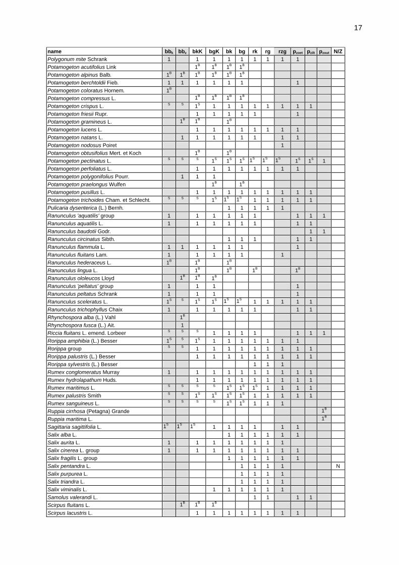
17

name bbk bbz bkK bgK bk bg rk rg rzg pzoet pzilt pzout N/ZPolygonum mite Schrank 1 1 1 1 1 1 1 1 1 Potamogeton acutifolius Link 1B 1B 1B 1B Potamogeton alpinus Balb. 1B 1B 1B 1B 1B 1B Potamogeton berchtoldii Fieb. 1 1 1 1 1 1 1 Potamogeton coloratus Hornem. 1B Potamogeton compressus L. 1B 1B 1B 1B Potamogeton crispus L. S S 1S 1 1 1 1 1 1 1 1 Potamogeton friesii Rupr. 1 1 1 1 1 1 Potamogeton gramineus L. 1B 1B 1B Potamogeton lucens L. 1 1 1 1 1 1 1 1 Potamogeton natans L. 1 1 1 1 1 1 1 1 Potamogeton nodosus Poiret 1 Potamogeton obtusifolius Mert. et Koch 1B 1B Potamogeton pectinatus L. S S S 1S 1S 1S 1S 1S 1S 1S 1S 1 Potamogeton perfoliatus L. 1 1 1 1 1 1 1 1 Potamogeton polygonifolius Pourr. 1 1 1 Potamogeton praelongus Wulfen 1B 1B Potamogeton pusillus L. 1 1 1 1 1 1 1 1 1 Potamogeton trichoides Cham. et Schlecht. S S S 1S 1S 1S 1 1 1 1 1 Pulicaria dysenterica (L.) Bernh. 1 1 1 1 1 Ranunculus 'aquatilis' group 1 1 1 1 1 1 1 1 1 Ranunculus aquatilis L. 1 1 1 1 1 1 1 1 Ranunculus baudotii Godr. 1 1 Ranunculus circinatus Sibth. 1 1 1 1 1 Ranunculus flammula L. 1 1 1 1 1 1 1 Ranunculus fluitans Lam. 1 1 1 1 1 1 Ranunculus hederaceus L. 1B 1B 1B Ranunculus lingua L. 1B 1B 1B 1B Ranunculus ololeucos Lloyd 1B 1B 1B Ranunculus 'peltatus' group 1 1 1 1 Ranunculus peltatus Schrank 1 1 1 1 Ranunculus sceleratus L. 1S S 1S 1S 1S 1S 1 1 1 1 1 Ranunculus trichophyllus Chaix 1 1 1 1 1 1 1 1 Rhynchospora alba (L.) Vahl 1B Rhynchospora fusca (L.) Ait. 1 Riccia fluitans L. emend. Lorbeer S S S 1 1 1 1 1 1 1 Rorippa amphibia (L.) Besser 1S S 1S 1 1 1 1 1 1 1 Rorippa group S S 1 1 1 1 1 1 1 1 1 Rorippa palustris (L.) Besser 1 1 1 1 1 1 1 1 1 Rorippa sylvestris (L.) Besser 1 1 1 Rumex conglomeratus Murray 1 1 1 1 1 1 1 1 1 1 Rumex hydrolapathum Huds. 1 1 1 1 1 1 1 1 1 Rumex maritimus L. S S S S 1S 1S 1S 1 1 1 1 Rumex palustris Smith S S 1S 1S 1S 1S 1 1 1 1 1 Rumex sanguineus L. S S S S 1S 1S 1 1 1 Ruppia cirrhosa (Petagna) Grande 1B Ruppia maritima L. 1B Sagittaria sagittifolia L. 1S 1S 1S 1 1 1 1 1 1 Salix alba L. 1 1 1 1 1 1 Salix aurita L. 1 1 1 1 1 1 1 1 Salix cinerea L. group 1 1 1 1 1 1 1 1 1 Salix fragilis L. group 1 1 1 1 1 1 Salix pentandra L. 1 1 1 1 N Salix purpurea L. 1 1 1 1 Salix triandra L. 1 1 1 1 Salix viminalis L. 1 1 1 1 1 1 Samolus valerandi L. 1 1 1 1 Scirpus fluitans L. 1B 1B 1B Scirpus lacustris L. 1 1 1 1 1 1 1 1

18

name bbk bbz bkK bgK bk bg rk rg rzg pzoet pzilt pzout N/ZScirpus maritimus L. S S 1 1 1 1 Scirpus sylvaticus L. 1 1 1 1 Scirpus tabernaemontani C.C. Gmel. 1 1 1 Scirpus triqueter L. 1 1 Scrophularia auriculata L. 1 1 1 1 1 1 1 1 1 Scrophularia nodosa L. 1 1 1 1 1 1 1 1 Scrophularia umbrosa Dum. 1 1 1 1 1 1 Scutellaria galericulata L. 1 1 1 1 1 1 1 1 Senecio aquaticus Hill 1 1 1 1 Senecio congestus (R. Brown) DC. 1 1 1 1 Senecio paludosus L. 1 1 Senecio sarracenicus L. 1 sewage fungus S S S S S S S S S S S Sium latifolium L. 1 1 Solanum dulcamara L. 1S S 1S 1S 1S 1S 1 1 1 1 1 Sparganium angustifolium Michaux 1B 1B Sparganium emersum Rehm. 1S 1S 1S 1 1 1 1 1 1 1 Sparganium erectum L. 1S S 1S 1 1 1 1 1 1 1 1 Sparganium natans L. 1B 1B 1B Sphagnum denticulatum Brid. 1 1 Sphagnum palustre L. 1 1 Sphagnum sp. 1 Spirodela polyrhiza (L.) Schleid. S S S S S 1S 1 1S Stachys palustris L. 1 1 1 1 1 1 1 1 1 Stellaria alsine Grimm 1 1 1 1 1 1 1 Stellaria nemorum L. 1 1 1 Stellaria palustris Retz. 1 1 1 1 1 1 1 1 Stratiotes aloides L. 1B 1B Symphytum officinale L. 1 1 1 1 1 1 1 1 Thalictrum flavum L. 1 1 1 1 1 1 Tolypella intricata (Trentepohl) Leonhardi 1B 1B Tolypella prolifera (Ziz) Leonhardi 1B 1B 1B Trichocolea tomentella (Ehrh.) Dum. 1 Trifolium fragiferum L. 1 1 1 1 1 Triglochin maritimum L. 1 1 Triglochin palustre L. 1 1 Typha angustifolia L. 1S 1S 1S 1S 1S 1S 1 1 1 1 Typha latifolia L. S S 1S 1S 1S 1S 1 1 1 1 1 Urtica dioica L. 1S S 1S 1S 1S 1S 1S 1S 1S 1S 1S 1S Utricularia australis R. Brown 1 1 Utricularia vulgaris L. 1B 1B 1B 1B 1B Vaccinium oxycoccos L. 1B Valeriana dioica L. 1 Valeriana repens Host. 1 1 1 1 1 1 1 1 1 Veronica anagallis-aquatica L. 1 1 1 1 1 1 1 1 1 1 Veronica beccabunga L. 1 1 1 1 1 1 1 1 Veronica longifolia L. 1 N Veronica scutellata L. 1 1 1 1 Viburnum opulus L. 1 1 1 Viola palustris L. 1 Wahlenbergia hederacea (L.) Reichenb. 1B Wolffia arrhiza (L.) Hork. ex Wimm. S S S 1S S 1S 1 Zannichellia palustris L. S S 1S 1S 1S 1S 1 1 1 Zannichellia palustris L. subsp. pedicellata (Wahlenb. et Rosén) Hegi

S S S S S S 1 1