report to the national measurement system policy unit...
TRANSCRIPT

NPL Report CMSC 42/04
Report to the National Measurement System Policy Unit, Department of Trade and Industry
Testing Continuous Modelling Software: Three Case Studies
T J Esward, K Lees, D Sayers, and L Wright
Revised June 2004

NPL Report CMSC 42/04
Testing Continuous Modelling Software: Three Case Studies
T J Esward(1), K Lees(2), D Sayers(3), and L Wright(1) (1): Centre for Mathematics and Scientific Computing, NPL (2): Centre for Electromagnetic and Time Metrology, NPL
(3): NAG Ltd., UK
March 2004
ABSTRACT This report describes three case studies of the testing of continuous modelling software. Where possible, the testing has been conducted by following the methodology outlined in the SSfM report “Testing Continuous Modelling Software” [1]. Where following this methodology has not been possible, the advice on alternative testing methods in the report [1] has been employed. The problems studied are:
• Testing boundary element method software for acoustic applications
• Testing finite integration technique software for electromagnetic applications
• Testing software that solves a system of ODEs to model semiconductor dislocations

NPL Report CMSC 42/04
© Crown Copyright 2004
Reproduced by Permission of the Controller of HMSO
ISSN 1471-0005
National Physical Laboratory Queens Road, Teddington, Middlesex, TW11 0LW
Extracts from this report may be reproduced provided the source is acknowledged and the extract is not taken out of context.
Approved on behalf of the Managing Director, NPL by Dave Rayner, Head of the Centre for Mathematics and Scientific Computing

NPL Report CMSC 42/04
Contents
1 Introduction...............................................................................................................1 2 Boundary element methods software........................................................................3
2.1 Details of the software ......................................................................................3 2.1.1 Mathematical formulation: The Helmholtz equation................................3 2.1.2 Circumventing the non-uniqueness problem ............................................4 2.1.3 Software implementations ........................................................................5
2.2 Test problem .....................................................................................................6 2.2.1 Generation of reference results .................................................................9
2.3 Test results ......................................................................................................12 2.3.1 Kirkup’s software ...................................................................................12 2.3.2 Forsythe’s CHIEF software ....................................................................15
2.4 Conclusions and recommendations for future work .......................................18 3 Computational electromagnetics software..............................................................19
3.1 Details of CST Microwave Studio..................................................................19 3.1.1 Special features of the software ..............................................................20
3.2 Test problems..................................................................................................21 3.3 Test results ......................................................................................................23
3.3.1 Scalable tests...........................................................................................23 3.3.2 Coaxial sensor tests.................................................................................26
3.4 Conclusions and extensions ............................................................................31 4 Semiconductor dislocation modelling software......................................................32
4.1 Details of the software ....................................................................................32 4.1.1 Physical problem.....................................................................................32 4.1.2 Mesh generation......................................................................................33 4.1.3 Mathematical formulation.......................................................................34 4.1.4 Solution method......................................................................................35 4.1.5 Software implementation........................................................................36
4.2 Test problem ...................................................................................................37 4.3 Test results ......................................................................................................39
4.3.1 Output quantity 1: Residuals of the ode systems....................................39 4.3.2 Output quantity 2: Free energy calculations ...........................................40 4.3.3 Output quantity 3: Difference between averaged and unaveraged boundary conditions................................................................................................43
4.4 Conclusions and extensions ............................................................................44 5 Conclusions.............................................................................................................46 6 References...............................................................................................................47
i

NPL Report CMSC 42/04
ii

NPL Report CMSC 42/04
1 Introduction This report describes three case studies of the testing of continuous modelling software. Where possible, the testing has been conducted by following the methodology outlined in the SSfM report “Testing Continuous Modelling Software” [1]. Where following this methodology has not been possible, the advice on alternative testing methods in the report [1] has been employed.
The problems examined involved the testing of a range of software, from popular commercial packages to in-house software with fully available source code. All of the software tested is either used on a regular basis at NPL or is being considered for regular usage. The application areas addressed are electromagnetics, acoustics, and stress analysis. The mathematical formulations of the problems include scalar and vector quantities subject to ordinary differential equations (odes) and partial differential equations (pdes). These choices show the broad range of applicability of the testing methods outlined in the report [1].
There are usually two important steps in the numerical solution of pde and odes: the approximation of the differential equations on the mesh, and the solution of the resulting system of equations. The testing methodology that has been developed for continuous modelling software aims to test both of these steps separately, wherever possible. The first step is tested using small-scale tests, and the second is tested using scalable tests. The methodology is illustrated by figure 1.
START: Choice of equation
Referenceresults
Reference data
Test software
Test results
Comparison
Scalable test definition
Small test definition
Test software
Reference results
Test results
Comparison
Figure 1: Methodology for testing continuous modelling software
Small-scale tests use a small number of mesh points to generate problems that can be solved analytically for a given approximation technique. The tests are not generally physically realistic as they require too many assumptions to hold. Small-scale tests check the formulation of the approximation to the pde because the system of equations that they produce is small and well-conditioned and so should be within the capabilities of the system solver. The definition of a small-scale test should always include the definition of its mesh because of the need to keep the test small-scale.
Where analytical solutions to pdes do exist, they can sometimes be characterised in terms of a number of variables, each a function of the input parameters. For example, many of the analytical solutions to the heat equation depend on α(λ, ρ, cp) = λ/ρcp, where λ is the thermal conductivity, ρ is the density, and cp is the specific heat capacity. This dependence means that problems with the same value of α but different individual values of λ, ρ, and cp will have the same solution. Any dependencies similar to this can
Page 1 of 48

NPL Report CMSC 42/04
be exploited to produce parametric families of input data for testing. A scalable test is a test based on an analytical pde or ode solution that has such a dependence.
Scalable tests test the solution of the full system of the equations where small-scale tests do not. Their results will be affected by problems with the formulation, but ideally the small-scale tests will have identified any such problems. Scalable tests are of interest to examine how the solution error varies with the changing input data.
Page 2 of 48

NPL Report CMSC 42/04
2 Boundary element methods software Boundary element methods are becoming increasingly popular for the solution of field prediction problems in a range of disciplines, including electromagnetic wave propagation, stress analysis, crack propagation, potential flow, and acoustics. This case study reports on the testing of three different software implementations of the boundary element method in acoustics.
Many problems of interest in acoustics concern the field radiated by a transducer or the field that is scattered by a target. In both these cases the acoustic domain of interest may be the whole of the fluid-filled space that surrounds the transducer or scatterer surface of interest. The need to represent a potentially infinite volume of air or water means that finite element methods cannot be applied easily to this kind of problem. Boundary element methods have an important contribution to make in the modelling of acoustic fields owing to their computational efficiency in solving problems with potentially infinite domains. The advantage of boundary element methods is that it is necessary only to define a mesh to represent the surface of the acoustic source and to formulate the mathematical problem to be solved as an integral equation. The integral equation relates the behaviour of points on the boundary element surface to acoustic quantities of interest, such as acoustic potential or pressure, at points in the exterior domain.
2.1 Details of the software 2.1.1 Mathematical formulation: The Helmholtz equation One of the most important partial differential equations in acoustics is the Helmholtz equation, which governs time-harmonic waves, that is, continuous waves that vibrate at a constant frequency.
For homogeneous media, the linear acoustic wave equation is
,012
2
22 =
∂∂
−∇tP
cP
where P is acoustic pressure, and c is the speed of sound in the medium. At any point in a fluid, time-harmonic waves oscillate sinusoidally according to
),exp( tipP ω=
where p is the complex pressure at the point of interest and ω is angular frequency (ω = 2πf where f is the frequency in Hertz). Complex p arises because the pressure possesses both amplitude and phase at any point of interest in the fluid. Combining these two equations produces the Helmholtz equation
,022 =+∇ pkp (1)
in which k = ω/c = 2π/λ is known as the wave number (λ is wavelength). For an explanation of methods of solving the Helmholtz equation, see Wu [2], Ch. 2, pp 10-27.
In general, the boundary conditions for the problem are given by an expression of the form
( ) ( ) ( ) ( ) ( )rrrrr γβα =+ nνp (2)
over the surface S of some volume V, where p is pressure, vn is the component of the particle velocity that is perpendicular to the surface of V and α, β and γ are functions of
Page 3 of 48

NPL Report CMSC 42/04
position r. The particle velocity is defined as the velocity of the motion of the fluid medium at a point as a result of the process of compression and rarefaction that the fluid undergoes. The type of problem is then defined by whether the results are required inside V (in which case the problem is an interior problem), or outside it (an exterior problem). For exterior problems, in addition to the conditions given in (2), a condition at infinity must be defined. A common choice is that all scattered and radiated waves are outgoing (called the Sommerfeld radiation condition).
The first step in using the boundary element method to solve the Helmholtz equation for interior or exterior problems is to reformulate (1) as a surface integral on the surface of V by using Green’s second theorem. This reformulation results in an equation of the form
( ) ( ) ( ) ( ) ( )∫∫ =−∂
∂S
qknS
k dS,GvpdSp,nG qrqrqqr
21 , (3)
where Gk is the (known) Green’s function for the Helmholtz equation given by the wave number k. The surface S is approximated by a set of boundary elements, an assumption is made about the behaviour of the pressure and velocity within each element, and the surface integral expression is applied to each element to produce a set of linear equations in p and vn. The conditions (2) are applied, and the resulting system is solved to give the pressure and normal velocity component on S.
Once the pressure and normal particle velocity are known on the surface of V, the pressure at points within the exterior domain can be calculated from
( ) ( ) ( ) ( ) ( )∫∫ −∂
∂=
Sqkn
Sq
q
k dS,GvdSp,nGp qrqqqrr .
For exterior problems, one of the limitations of the boundary element method is that equation (3) does not have a unique solution at the eigenfrequencies of the interior Dirichlet problem, because the left hand side of equation (3) is singular for these frequencies (in acoustics the Dirichlet boundary condition implies that the pressure p is known on the boundary of V and the particle velocity vn is unknown, whereas the Neumann boundary condition implies that the particle velocity is prescribed on the surface). In addition to the non-uniqueness, the left hand side of equation (3) is ill-conditioned for frequencies close to the eigenfrequencies, making accurate solution of the problem very difficult. It should also be noted that, as the frequency increases, the eigenfrequencies become more closely spaced. The non-uniqueness problem will be illustrated in section 2.2.1.
A more extensive explanation of these issues is given in Wu [2], pp 24-27. A discussion of non-existence and non-uniqueness problems associated with integral equation methods in acoustics can be found in Benthien and Schenck [3].
2.1.2 Circumventing the non-uniqueness problem Two of the main methods for overcoming the non-uniqueness problem described in the previous section are due to Schenck [4] and Burton and Miller [5]. A complete description of each approach is given in the papers by these authors, but an outline of each is given below.
Schenk’s method, known as CHIEF
CHIEF stands for Combined Helmholtz Integral Equation Formulation. In this method
Page 4 of 48

NPL Report CMSC 42/04
additional constraining interior points are defined within the volume V, and the pressure at each of these points is constrained to be zero. These points are often called CHIEF points and the associated equations are known as the CHIEF equations.
The aim of using these additional constraints is that the extra zero-pressure conditions produce a unique solution to the exterior problem. However, if the solution to the interior Dirichlet problem is zero at the chosen CHIEF point, the additional constraint will have no effect, and so care must be taken when choosing CHIEF points. In addition, as frequency increases more CHIEF points are required and it becomes more difficult to choose suitable points. It is not always clear how many CHIEF points are needed and where they should be placed. However, at low frequencies the CHIEF method has been shown to produce reliable results for the exterior Helmholtz problem (see Wu [2]).
Burton and Miller method
This method is an improved formulation of the surface Helmholtz equation. The formulation is obtained by differentiating the surface Helmholtz equation with respect to the normal to the boundary and forming a linear combination of the surface Helmholtz equation and the differentiated equation. Further details are given in Burton and Miller [5] and Kirkup [6, 7]. A coupling constant µ is required on both sides of the improved equation formulation to ensure that the relative contribution from all of the terms in the integral equation are balanced, whatever value the wave number k takes. Kirkup [7] points out that this is achieved by setting µ approximately equal to 1/k. In the work reported here a coupling constant of µ = i/(k + 1) has been used, in accordance with Kirkup’s practice in his test examples ([7], p 91).
2.1.3 Software implementations Three software packages suitable for solving the external Helmholtz problem were available: the PAFEC vibroacoustics combined finite element and boundary element software, an implementation of the Burton and Miller approach by Kirkup [7] and a realisation of the CHIEF method in Matlab by Forsythe [8].
PAFEC is a general finite element software package that is particularly well-suited to applications in vibroacoustics. More information about PAFEC can be found on their website at http://www.vibroacoustics.co.uk/index.htm. As was pointed out earlier, the representation of the fluid in external Helmholtz problems can provide a substantial challenge for numerical solution techniques. PAFEC has a range of methods for meeting this challenge. It offers several boundary element methods, including the CHIEF method described earlier and a finite element method using what are known as wave envelope elements. More information about such elements can be found in Astley et al [9-11] and Cremers et al [12].
Kirkup’s boundary element software is a realisation of the boundary element method that includes an implementation of the Burton and Miller approach to the solution of exterior Helmholtz problems. The programming language employed is FORTRAN77 and the source code is available. The code and its use are described at length in Kirkup [7]. Further information about the software and links to acoustic modelling resources can be found at http://www.soundsoft.demon.co.uk/. An order form for the software is available from this site.
Forsythe’s Matlab realisation of CHIEF is a boundary element solver that uses the CHIEF method for external Helmholtz problems. The software itself is also known as CHIEF. The version of CHIEF for Matlab that was used in this study was developed by
Page 5 of 48
NPL Report CMSC 42/04
S.E Forsythe of the United States’ Naval Undersea Warfare Center, Newport, Rhode Island, USA [8]. Forsythe makes the Matlab version of the code available to interested parties in the form of a suite of Matlab m-files and he can be contacted by e-mail at [email protected].
2.2 Test problem Only a limited range of idealised acoustic problems is easily amenable to analytical solutions. This lack of analytical solutions makes the use of scalable tests as described in the software testing methodology [1] difficult. Instead, reference software has been chosen as a preferable option. As was mentioned in section 2.1.3, PAFEC has two methods for solving external Helmholtz problems that are derived from different types of discrete approximation. The independence of the two methods means that they can be used to validate one another’s results. This validation has made it possible to use PAFEC as reference software for this study.
The small-scale tests recommended as the second step of the methodology [1] are not generally suitable for boundary element methods. The software tested here assumes that the pressure remains constant within each boundary element, which severely limits the range of problems for which a reasonably accurate solution can be found using a small number of elements.
The choice of test problem was made on the basis of the rationale set out below.
• The test should be as far as possible a test of the software itself and not of the user’s ability to employ the software or to implement novel problems using the software.
• The test problem should be within the expected capabilities of each of the three software packages and should not require very large or very dense meshes since this study is a test of the algorithms used to solve the problem rather than of meshing capabilities.
• To compare the CHIEF and Burton and Miller method an external Helmholtz problem should be chosen involving a frequency at which the non-uniqueness problem exists.
• The problem should be restricted to frequencies that are low enough to require only a limited number of CHIEF points to produce an accurate result.
• If possible, the test problem should be based on the kinds of routines which the suppliers of the software packages had themselves used to test their software and which they had made available to potential users.
• The test problem should require only relatively straightforward edits to existing software routines, for example, to change the values of input parameters, to avoid the need to make any edits of the routines which might compromise the kernel of the software under test.
Given the requirements set out above it was decided to define a test problem as follows:
• Calculate the far-field scattered acoustic pressure amplitude (commonly known as the directional response) arising from a single frequency, continuous wave point source irradiating a 1 m radius rigid sphere.
• The point source is to be located 8 m from the centre of the sphere.
Page 6 of 48

NPL Report CMSC 42/04
• The fluid surrounding the sphere is water.
• Two frequencies are to be analysed, one where the non-uniqueness problem is not an issue and one where it is. For spheres this latter case occurs where ka, the product of the wave number and the sphere radius, is equal to π.
Far-field, in this case, means “sufficiently far from the source and scatterer that any surface interference effects have died away”. The boundary conditions on the surface of the sphere are given by the values of the pressure due to the point source on the surface of the sphere. The pressure at a distance r from the point source (before scattering) is given by P(f)exp(-ikr)/r, where P(f) is the source strength at the frequency of interest.
The material parameters needed for the solution of the external Helmholtz problem are the speed of sound in the medium and the density of the medium. For fluids such as water these quantities are related by
,Bcρ
=
where c is the speed of sound in m s-1, ρ is density in kg m-3 and B is the bulk modulus of the fluid in Pa. Both Kirkup’s and Forsythe’s software require the user to input the speed of sound and the density. PAFEC requires the bulk modulus and density and then calculates sound speed itself. Table 1 sets out the parameters that define the problems. The exact value of frequency employed in test 1 was 238.73241 Hz.
Test 1 Test 2 Frequency f (Hz) 238.7 750 Sphere radius a (m) 1 1 Sound speed c (m s-1) 1500 1500 Density ρ (kg m-3) 1026 1026 Bulk modulus B (GPa) 2.3085 2.3085 Wavelength λ (m) 6.284 2.000 ka 1.000 3.141
Table 1. Input parameters of test problems
If the acoustic axis of the source-sphere system is defined as the line joining the point source to the centre of the sphere, then the problem has axial symmetry and the exploitation of this symmetry would allow the most efficient solution of the problem. PAFEC and the Kirkup software can both solve axisymmetric problems. However, the Forsythe CHIEF software does not offer an axisymmetric solver and so all problems must be solved in three dimensions. In order that the same problem is solved by the two packages under test, the symmetry has not been exploited in the tests of the Kirkup and Forsythe. The axisymmetric solver has been used in the generation of the reference data because if the results are to be regarded as sufficiently accurate to be reference results, their method of calculation must be irrelevant.
A further approximation arises in relation to the definition of the far field. Kirkup’s and Forsythe’s software both require definition of the exact location of the points at which results are calculated. PAFEC has an option that calculates the far field results without the location of the far field being defined. For the purposes of this test, it is assumed that the far field lies 1,000 m from the spherical surface. This assumption was explored
Page 7 of 48

NPL Report CMSC 42/04
further during the generation of the reference data, as will be described in section 2.2.1. The test problem is shown in figure 1.
Figure 1: Diagram of test problem (not to scale)
The three software packages use different definitions of a point source. To allow direct comparison of the results of the three software packages, it is necessary to ensure consistent scaling of the results. The scaling factor depends on whether the point source is treated as a pressure source or a velocity source. For single frequency periodic sources, as are used in this problem, there is a simple relationship between the velocity potential and the pressure. Following Skudrzyk (1971, p 279) this is
,cki
pρ
ϕ =
where φ is the velocity potential. For direct comparison with PAFEC it is necessary to divide the predicted pressure amplitudes by kρc. These factors vary between approximately 106 kg m-3 s-1 and approximately 107 kg m-3 s-1 depending on frequency and which factor is considered.
To compare predictions from the software packages, the root mean square (RMS) difference between the results is often employed in this report. Scaling the results by a constant factor of the order of 106 leads to the possibility of rounding errors
Page 8 of 48

NPL Report CMSC 42/04
contributing to the RMS difference calculation, and this should be taken into account when considering the results presented here.
2.2.1 Generation of reference results The results were generated using PAFEC version 8.6. The test problem was analysed using both the boundary element and the wave envelope element method. As these are two distinctly different mathematical approaches to the problem of interest, the results from each method act as a check upon each other.
The first test was to derive the far field scattered pressure field (also known as directivity) using the CHIEF boundary element method for the two test frequencies. PAFEC calculates the far field pressure as
( ),lim rprr ∞→
(4)
on the assumption that this limit exists and is unique. This definition means that if the pressure at r = 1000 m is to be a good approximation to the far-field pressure, the limit given by (4) divided by a factor of 1000 should equal the calculated scattered pressure at 1000m.
As the problem is axisymmetric it was sufficient to model the sphere surface as a semicircle of unit radius. 17 equi-spaced nodes (angular separation 11.25 degrees) were placed on this semi-circle. In general, a mesh for solving an acoustic scattering problem requires the maximum element length to be at most 1/3 of the wavelength. As the shortest wavelength employed in the analysis is 2 m and the circumference of the semi-circle is π m, the chosen mesh was considered to be sufficiently dense for both frequencies. Tests with denser meshes showed that this was in fact the case: the tests with denser meshes produced the same results. Three CHIEF points were used in the region inside the spherical surface.
Results were requested at intervals of one degree on a circle centred on the origin of the co-ordinate system, which is taken to be where the centre of the sphere is located. Owing to the symmetrical nature of the problem, results in the angular range 0 to 180 degrees are mirrored by those in the range 180 to 360 degrees, so that in the figures that follow only the angular range from 0 to 180 degrees is shown.
A second analysis was performed in which results were requested at a specific distance of 1000 m from the origin to allow direct comparison with Forsythe’s and Kirkup’s software. The results of the analysis of the scattered field at 1000 m and the far field results scaled by a factor of 1000 are compared in figures 2 and 3.
Figure 2 presents the results of the 238.7 Hz analysis and figure 3 displays the results of the 750 Hz analysis. Note that for both frequencies, on the scale of the graphs, the far field and 1000 m results cannot be distinguished. The root mean square difference between the pairs of normalised results is 1.7 × 10⁻⁸ at 238.7 Hz and 5.3 × 10⁻⁸ at 750 Hz. These results show that a distance of 1000 m is a good approximation to the far field.
Page 9 of 48

NPL Report CMSC 42/04
0.00E+00
1.00E-05
2.00E-05
3.00E-05
4.00E-05
5.00E-05
6.00E-05
7.00E-05
0 20 40 60 80 100 120 140 160 180Angle (degrees)
Pres
sure
am
plitu
de (P
a)Scaled far field 1000 m
Figure 2: Comparison between the PAFEC boundary element scaled far field response and 1000 m results, compared at 238.7 Hz.
0.00E+00
2.00E-05
4.00E-05
6.00E-05
8.00E-05
1.00E-04
1.20E-04
1.40E-04
1.60E-04
0 20 40 60 80 100 120 140 160 180
Angle (degrees)
Pres
sure
am
plitu
de (P
a)
Scaled far field 1000 m
Figure 3: Comparison between the PAFEC boundary element scaled far field response and 1000 m results, compared at 750 Hz.
The results of these calculations were further validated by comparing them with the results of a model of the same problem using wave envelope elements. Plots of the two sets of results showed no visible difference between them at 238.7 Hz and very little difference at 750 Hz. For the 238.7 Hz case the RMS difference between the two sets of results was 2.6 × 10⁻⁸ and at 750 Hz it was 3 × 10⁻⁷. These calculations validated the reference results and increased confidence that the implementation of the CHIEF method in PAFEC could be used to generate reference results for these problems.
Page 10 of 48

NPL Report CMSC 42/04
The next study performed with the PAFEC software was an investigation of the effect of omitting CHIEF points for both the low and the high frequency case. This was to check that the problem requiring CHIEF points had been defined correctly. The expectation is that the omission of CHIEF points would have no effect on the 238.7 Hz results (ka = 1) but that the prediction at 750 Hz (ka = π) would fail. In practice, no difference between the two cases was found at 238.7 Hz. However, figure 4 presents the 750 Hz prediction, which shows that at this frequency the analysis clearly fails if no CHIEF points are used. These results show that CHIEF points are required for the solution of the 750 Hz problem, and that the points that were chosen gave a good solution.
19.34
19.36
19.38
19.40
19.42
19.44
19.46
19.48
19.50
19.52
19.54
0 20 40 60 80 100 120 140 160 180
Angle (degrees)
Pres
sure
am
plitu
de (P
a)
Figure 4: PAFEC boundary element solution calculated without CHIEF points, far field directional response at 750 Hz.
The results of the previous tests have only shown the scattered field, rather than the combined field of the source and its scattering. PAFEC allows the calculation of the total field at the point of interest, and this calculation can also be performed using the Kirkup software. Thus it was decided to generate the total field for comparison with the Kirkup results.
The total pressure field at the 1000 m position was calculated for both test frequencies using the CHIEF method with PAFEC. Since acoustic pressure is a complex quantity, constructive and destructive interference effects occur, as waves of differing phase, such as the source and its scattered field, are summed. Figure 5 shows the results of the total pressure field calculation for 238.7 Hz and 750 Hz. The effects of constructive and destructive interference between the two acoustic sources are clearly identified, and shown to be frequency dependent as expected.
Page 11 of 48

NPL Report CMSC 42/04
0.00E+00
2.00E-04
4.00E-04
6.00E-04
8.00E-04
1.00E-03
1.20E-03
0 20 40 60 80 100 120 140 160 180
Angle (degrees)
Pres
sure
am
plitu
de (P
a)238.7 Hz 750 Hz
Figure 5: Total pressure field at 1000 m at 238.7 Hz and 750 Hz calculated using PAFEC
2.3 Test results Throughout this section, RMS values for comparisons between the various sets of results are given. These values are presented in table 2 in section 2.4 for ease of further comparison. All sets of results consisted of pressure amplitudes calculated at 181 equally spaced points around half of the 1000m radius circle indicated in figure 1.
2.3.1 Kirkup’s software Following creation of the reference results, the scattering problem was analysed using Kirkup’s FORTRAN software, which employs the Burton and Miller method for the solution of the exterior Helmholtz problem. The routine employed computes the solution to the Helmholtz equation exterior to a general closed surface in a three-dimensional domain.
The spherical surface was discretised into a mesh of planar triangular elements, as is required by the software for all three-dimensional analyses. Kirkup’s software has no automatic meshing facilities, and each node and element has to be defined individually by the user of the software and entered either via a text file or directly into the source code. The first mesh that was used contained 134 nodes joined together to form 264 elements, as shown in figure 6. This is a more coarse mesh than that used to generate the reference results, although it still passes the “three elements per wavelength” criterion mentioned in section 2.2.1. Even with this number of elements, the mesh is no more than an approximate representation of a sphere, owing to the fact that each element forms a plane surface. The number of elements that can be used in Kirkup’s software is limited by the need to store an N by N matrix when using a mesh with N elements.
Page 12 of 48

NPL Report CMSC 42/04
Figure 6: Coarse mesh used in Kirkup’s software to calculate the pressure field
A more dense mesh of the sphere was created, consisting of 308 nodes and 612 elements, in order to compare the effects of mesh density on the results. Comparisons between the predictions from the two meshes are presented in figures 7 and 8. Figure 7 shows the 238.7 Hz results for the scattered field for the two Kirkup meshes and the reference results. Note that the denser Kirkup mesh produces closer agreement with the reference results at this frequency.
Figure 8 shows the same comparison at 750 Hz, and the denser mesh achieved better agreement with the reference results than the original mesh, especially in the regions close to 60 degrees and 180 degrees. The improvement in agreement with increasing mesh density probably means that the differences between the test results and the reference results are due to an insufficiently dense mesh, rather than any fundamental deficiencies in the software.
The RMS differences between the Kirkup results and the reference results for the scattered field predictions at 238.7 Hz were 1.86 × 10⁻⁶ (coarse mesh) and 8.82 × 10⁻⁷ (fine mesh). The equivalent 750 Hz results were 2.04 × 10⁻⁶ (coarse mesh) and 1.88 × 10⁻⁶ (fine mesh).
The dense mesh was also used to derive the total pressure (i.e. the field scattered by the sphere and the field arising directly from the point source) at both 238.7 Hz and 750 Hz for comparison with the reference results. These results are shown in figures 9 and 10. Considering the results as a function of angle, the differences between the reference total field and the Kirkup total field never exceed 0.5% at any angle at 238.7 Hz and exceed 1% at 750 Hz only in the region around 20 degrees.
Page 13 of 48

NPL Report CMSC 42/04
For the total pressure field predictions using the Kirkup fine mesh the RMS differences were 1.29 × 10⁻⁶ at 238.7 Hz and 4.20 × 10⁻⁶ at 750 Hz. It should be noted that since the pressure due to a point source is given by an analytical expression, it is expected that the error in the total field and the error in the scattered field will be approximately equal. The figures show this to be the case.
0.00E+00
1.00E-05
2.00E-05
3.00E-05
4.00E-05
5.00E-05
6.00E-05
7.00E-05
0 20 40 60 80 100 120 140 160 180Angle (degrees)
Pres
sure
am
plitu
de (P
a)
Kirkup dense mesh Kirkup coarse mesh Reference result
Figure 7: Results from Kirkup’s software using coarse and dense meshes compared with reference results for scattered pressure at 238.7 Hz.
0.00E+00
2.00E-05
4.00E-05
6.00E-05
8.00E-05
1.00E-04
1.20E-04
1.40E-04
1.60E-04
0 20 40 60 80 100 120 140 160 180
Angle (degrees)
Pres
sure
am
plitu
de (P
a)
Kirkup dense mesh Kirkup coarse mesh Reference result
Figure 8: Results from Kirkup’s software using coarse and dense meshes compared with reference results for scattered pressure at 750 Hz.
Page 14 of 48

NPL Report CMSC 42/04
0.00E+00
2.00E-04
4.00E-04
6.00E-04
8.00E-04
1.00E-03
1.20E-03
0 20 40 60 80 100 120 140 160 180
Angle (degrees)
Tota
l pre
ssur
e (P
a)
Kirkup dense mesh Reference result
Figure 9: Results from Kirkup’s software using the dense mesh compared with reference results for total pressure at 238.7 Hz.
0.00E+00
2.00E-04
4.00E-04
6.00E-04
8.00E-04
1.00E-03
1.20E-03
0 20 40 60 80 100 120 140 160 180
Angle (degrees)
Tota
l pre
ssur
e am
plitu
de (P
a)
Kirkup dense mesh Reference result
Figure 10: Results from Kirkup’s software using the dense mesh compared with reference results for total pressure at 750 Hz.
2.3.2 Forsythe’s CHIEF software The software used for the work reported here is version 2.0. Matlab version 6.5.1 was employed throughout. The software’s automatic meshing facilities were employed to generate the mesh. Boundary element patches in Forsythe’s software are in general quadrilaterals, although for some geometries triangles may be needed to complete the required shape in a satisfactory manner. The mesh that was employed for the current
Page 15 of 48

NPL Report CMSC 42/04
analysis is shown in figure 11. The mesh consists of 34 strips of 24 elements, and so it has almost the same mesh size as the mesh used to generate the reference results. The mesh has a total of 816 elements, considerably more than the finer of the meshes used with Kirkup’s software. Once again, given that at 750 Hz the wavelength is 2 m, the mesh is a more than adequate discretisation of a sphere of 1 m radius for the test problems.
Figure 11: Mesh used in Forsythe’s CHIEF software to calculate the scattered pressure field
The first study performed with Forsythe’s software was a comparison of the 238.7 Hz results for the scattered pressure with and without the inclusion of CHIEF points with the reference results. Since this frequency is not expected to have non-uniqueness problems, the results should be independent of the presence of CHIEF points. The CHIEF points used were the same three points as those used successfully during the generation of the reference results.
Figure 12 shows the results. Note that on the scale of the graph it is not possible to distinguish between the reference results and those for the Forsythe code. The RMS differences between the reference results and Forsythe 238.7 Hz results shown in figure 12 are for the case of the Forsythe prediction 5.04 × 10⁻⁸ without CHIEF points and 5.05 × 10⁻⁸ with the inclusion of CHIEF points.
The results shown in figure 12 are behaving in the expected manner: the presence of CHIEF points should not decrease the accuracy of the solution since the equations imposed at the CHIEF points are consistent with the equations generated by the surface integral, and so the solution accuracy should not be compromised.
Page 16 of 48

NPL Report CMSC 42/04
0.00E+00
1.00E-05
2.00E-05
3.00E-05
4.00E-05
5.00E-05
6.00E-05
7.00E-05
0 20 40 60 80 100 120 140 160 180Angle (degrees)
Pres
sure
am
plitu
de (P
a)
Forsythe without CHIEF points Forsythe with CHIEF points Reference result
Figure 12: Comparison of reference results and results of Forsythe’s software for scattered pressures at 238.7 Hz
The next series of tests calculated the scattered pressures at 750 Hz with and without CHIEF points. These results are shown in figure 13. It is clear that at this frequency the failure to include CHIEF points produces an erroneous result, as would be expected. The RMS differences between the Forsythe and reference results at 750 Hz are 3.78 × 10⁻⁵ for the calculation without CHIEF points and 2.45 × 10⁻⁷ for the calculation that includes CHIEF points.
0.00E+00
5.00E-05
1.00E-04
1.50E-04
2.00E-04
2.50E-04
0 20 40 60 80 100 120 140 160 180Angle (degrees)
Pres
sure
am
plitu
de (P
a)
Forsythe without CHIEF points Forsythe with CHIEF points Reference result
Figure 13: Comparison of reference results and results of Forsythe’s software for scattered pressures at 750 Hz
Page 17 of 48

NPL Report CMSC 42/04
2.4 Conclusions and recommendations for future work This study has concentrated on a simple low frequency acoustic scattering problem as a means of comparing the CHIEF and Burton and Miller methods of solving the exterior Helmholtz problem. The approach has been to define as simple a problem as possible to test the software itself. The aim has not been to test the skill of the user in getting the best performance possible out of the software in question, nor to recommend software to tackle a particular problem.
The reference results were generated using PAFEC as reference software. PAFEC was chosen to generate the reference results because it had two independent methods of calculating the required results, and so the results of the two methods could be used to validate one another. The RMS difference between the reference results calculated using the two methods was 2.6 × 10⁻⁸ at 238.7 Hz, and at 750 Hz it was 3.0 × 10⁻⁷.
Table 2 summarises the results for RMS differences between the test results and the reference results. The agreement with the reference results was always closer for Forsythe’s software than for Kirkup’s software in the case of calculations of scattered fields, provided that CHIEF points were used were necessary.
Kirkup’s software produced good agreement with the PAFEC reference results, especially for the total pressure fields at 1000 m. Agreement for the scattered pressure alone was slightly less good, especially in the 750 Hz case, although the overall shape of the scattering pattern was represented successfully. Forsythe’s software produced good agreement of the scattered pressure fields with the reference results in all cases, provided that CHIEF points were used when needed.
Frequency (Hz) Software, mesh and field details
238.7 750
Kirkup, coarse mesh, scattered field 1.86 × 10⁻⁶ 2.04 × 10⁻⁶
Kirkup, fine mesh, scattered field 8.82 × 10⁻⁷ 1.88 × 10⁻⁶
Forsythe, no CHIEF points, scattered field 5.04 × 10⁻⁸ 3.78 × 10⁻⁵
Forsythe, CHIEF points, scattered field 5.05 × 10⁻⁸ 2.45 × 10⁻⁷
Kirkup, fine mesh, total field 1.29 × 10⁻⁶ 4.20 × 10⁻⁶
Table 2: RMS differences between the reference results and the various sets of test results.
There are a number of aspects of the use of continuous modelling software that have not formed part of this study, such as the optimisation of meshes, the choice of number and location of CHIEF points, and the choice of coupling constant in the Burton and Miller formulation. These aspects could form the subject of further investigations.
Page 18 of 48

NPL Report CMSC 42/04
3 Computational electromagnetics software Much of the computational electromagnetic modelling work undertaken at NPL involves simulation of experiments, often with a view to carrying out sensitivity analyses and determining uncertainties associated with experimental results. This focus means that it is important to ensure that modelling errors do not add significantly to the uncertainty, which means that software testing is a key concern for this work.
NPL has already carried out a number of testing and benchmarking exercises on some of its CEM codes. An extensive inter-comparison [14] of four different packages using four different calculation methods led to an objective view of the strengths and weaknesses of each, and also provided several sets of reference data that could be used for testing other packages. The software results were further validated against measurement data.
CST’s MicroWave Studio® (MWS) [15] was not included in this earlier inter-comparison, but is used extensively at NPL. The work described in this case study is intended to apply the software testing methodology [1] to MWS.
3.1 Details of CST Microwave Studio The MWS manual [15] says that:
“The software is a general-purpose electromagnetic simulator based on the Finite Integration Technique (FIT), first proposed by Weiland in 1976/1977 [16]. This numerical method provides a universal spatial discretisation scheme, applicable to various electromagnetic problems, ranging from static field calculations to high frequency applications in time or frequency domain.”
FIT uses the integral form of Maxwell’s equations
∫∫ ∫∫ ∫∫ ∫
∂∂
∂∂
=⋅=⋅
⋅⎟⎠⎞
⎜⎝⎛ +
∂
∂=⋅⋅
∂
∂−=⋅
VV V
A AA A
ddVd
dt
ddt
d
0ABAD
AJDsHABsE
ρ (5)
where:
E is the electric field measured in Vm-1 ,
B is the magnetic field measured in T,
H = B/µ where µ is the magnetic permeability measured in NA-2,
D = εE where ε is the electric permittivity, measured in Fm-1,
J is the vector current density measured in Am-2, and
ρ is the charge density in Cm-3.
These equations are applied individually to every cell in a pair of offset finite volume meshes. One mesh is used for calculation of the electric field and the other is used for calculation of the magnetic field. A similar technique using a pair of offset finite volume meshes is often used in computational fluid dynamics for calculation of pressures and velocities from integrated forms of the laws of conservation of mass and momentum.
Page 19 of 48

NPL Report CMSC 42/04
The software can be used for time domain problems, frequency domain problems, and eigenvalue problems. Central differences are used to approximate the time derivatives in time domain problems, giving an explicit method for solution of the discretised form of the equations (5) that does not require iterative techniques. The times at which the electric and magnetic fields are calculated are offset from one another by half a time step, called a staggered leapfrog technique, which provides a stable and accurate solution at little computational cost.
If it is assumed that the current densities are zero, and that E and B are periodic in time so that E = E0eiωt and B = B0eiωt, the system of equations (5) leads to an eigenvalue problem of the form
02
02 ΕΕ µεω−=∇ (6)
with appropriate boundary conditions. The eigenmode solver in MWS®, which has been tested in this work, uses a Krylov subspace method [17] to solve the discretised form of the eigenvalue problem. Krylov subspace methods are commonly used for solution of large-scale eigenvalue problems, particularly for large sparse symmetric matrices such as those generated by the FIT, because they require a small amount of storage for the matrix terms and converge more quickly than some of the alternative iterative methods.
The frequency domain problems are similar in form to the eigenvalue problems. The electrical field is written as the sum of a set of terms of the form E0eiωt, and the field equations become
( ) JEE ωωµ i−=−×∇×∇ 02
01 ,
where all terms are as defined above. This formulation is particularly useful for problems that only require a few frequencies to describe them sufficiently accurately. According to the manual, MWS is not suitable for solving frequency-domain problems involving lossy materials.
Another useful feature of MWS is its ability to calculate Q-factors. The Q- or quality factor of a resonant system is a measure of the ratio of the energy stored in the system to the energy lost during one cycle of operation. This is a useful property for filter design as it gives a measure of the broadening of the spectral behaviour of a resonating system. Additionally the phase angle of the complex permittivity of a dielectric is approximately inversely proportional to the Q-factor, which is a useful property for measurement of complex permittivity.
3.1.1 Special features of the software MWS includes an automatic mesh generation tool. Electromagnetic computations can be extremely sensitive to mesh density, and they generally require a certain number of volumes per wavelength to capture the behaviour correctly. The automatic meshing tool calculates the wavelength from the input quantities, and creates a suitable mesh for the problem. Whilst the automatic meshing can be turned off, the recommended way of using the software is to employ automatic meshing.
The requirement for multiple volumes per wavelength makes “single element” tests as outlined in the software testing methodology [1] impossible to define. This has meant that this part of the software testing methodology has had to be neglected for this case study.
Page 20 of 48

NPL Report CMSC 42/04
Whilst automatic meshing is a generally useful tool, it does mean that in general the user does not have direct control over the mesh unless the automatic meshing tool is turned off. This makes the “scalable” tests more difficult to control. However, the scalable tests that have been chosen are of constant wavelength, so in theory the meshes for the tests should be sufficiently similar that any significant changes in the results should not have been caused by the changes in the mesh.
MWS also includes an adaptive meshing tool. This tool runs models with a series of progressively finer meshes to ensure that the model results have converged. This enables the user to get a feel for how reliable the results are likely to be. If the results produced from models with different mesh densities have converged to a single solution, the results are more likely to be accurate. The adaptive meshing tool has been used in some of the tests in order to maximise the likelihood of obtaining converged results.
MWS is able to model curved surfaces accurately through its use of the Perfect Boundary ApproximationTM (PBA) technique [18]. Many discretisation methods for continuous models require meshes to be constructed using straight lines, and in many cases this requirement leads to a poor approximation to the shape of the true surface. The PBA technique does not require boundaries of the computational domain to be defined by boundaries of the mesh volumes. Instead a second-order approximation is developed using the exact geometry of the boundary and partially-filled volumes to produce an accurate approximation for problems involving curved surfaces. This property of MWS is particularly relevant to the work described here because the test geometry of the scalable tests is a sphere, which would cause problems for some approximation methods.
3.2 Test problems Two sets of test problems were used. The first set had an analytical solution [19] and so reference data and results were easy to generate. The second set had been used previously [14] for intercomparison of different software packages. During this intercomparison exercise, identical results were obtained using several different mathematical techniques, and so the results can be regarded as sufficiently accurate to be used as reference results.
The first set of test problems was to find the first three resonant frequencies of a spherical cavity of radius a and the Q-factor for the lowest mode. The analytical solution for this problem [19] can be found by seeking separable solutions to the problem (5), applying boundary conditions that various components of the electric or magnetic field be zero on r = a, and calculating the eigenvalues from the resulting equations. Two types of eigenfunction exist: one type in which the electrical field has a zero radial component (called the transverse electric or TE solution), and one type in which the magnetic field has a zero radial component (called the transverse magnetic or TM solution). The eigenvalues corresponding to both types of eigenfunction are expressed as the solutions to equations involving spherical Bessel functions and their derivatives.
The expressions for the resonant frequencies and the Q factor are
Page 21 of 48

NPL Report CMSC 42/04
( ) ( )
( )( ) ⎥
⎥⎦
⎤
⎢⎢⎣
⎡
′−=
===′=′=′===
====
′==
211
0110011
00
312111
312111
212
973487037442988676354934
232132110
22
ζµπσµ
εεεµµµζζζζζζ
πω
εµπ
ζ
εµπ
ζ
TMr
rr
rr
npTMmnp
rr
npTEmnp
faQ
,,,.,.,.,.,.,.
f,...,,p,...,,,n,n,...,,m
,a
cf,
a
cf
where σ is the conductivity of the material in Ω-1 m-1, c = 2.998 ×10⁸ ms-1 is the speed of light in vacuo, µ0 is the magnetic permeability of free space = 4π×10-7 NA-2 and ε0 is the electric permittivity of free space = 1/( µ0c2) Fm-1. µr and εr are called the relative permeability and the relative permittivity respectively, are dimensionless, and have a minimum value of 1.0. The reference solution for the Q factor was quite difficult to obtain, due to the varying notation of the sources consulted and the problems converting between absolute and relative permittivity and permeability.
The dependence of the resonant frequencies on the radius of the sphere and the relative permeability and permittivity means that if the product a√(εr µr) is kept constant but the individual components are changed, the frequencies will stay fixed. This property meant that a set of tests could be designed expecting the same result but with a range of different input parameters a, εr and µr. The conductivity was held fixed throughout at 5 × 10⁷ Ω-1 m-1.
The initial test plan was to vary the radius of the sphere between 10-3 m and 103 m, vary the permittivity and permeability between 1 and 1012, and keep the product a√(εr µr) fixed at 106 m. Each of the values used was an integer power of 10 to make the parameter input straightforward. The original choice of individual combinations will not be listed in full, for reasons that will be explained in section 3.3.1. It should be noted that these values of relative permittivity and permeability were extremely unrealistic: the permeability and permittivity of real materials would be expected to lie in the range 1-103, with values higher than this being comparatively rare. However, the aim of this set of software tests was not to simulate real situations, it was to investigate how the software would behave under extreme conditions.
The second set of tests simulated coaxial sensors, used to measure complex permittivity for soft materials and liquids. The sensors pass an electromagnetic signal down a coaxial cable. The signal is reflected at the boundary between one end of the cable and the dielectric substance being measured. The reflection causes the signal’s amplitude and phase to change, and the sensor measures this change in the form of a reflection coefficient Γ such that reflected signal = Γ × original signal. If |Γ|<1 then the energy has been coupled into the substance. The complex permittivity of the substance can be calculated from Γ.
The models used in the tests were time domain models of a coaxial sensor in contact with a substance of known complex permittivity. The tests can be grouped into three subsets, consisting of models of:
1. A coaxial sensor and a cylinder of air of radius 35 mm and length 60 mm at
Page 22 of 48

NPL Report CMSC 42/04
frequencies every 0.1 GHz between 0.1 GHz and 2.0 GHz,
2. A coaxial sensor and a cylinder of dielectric material of various thicknesses between 0.07 mm and 9.97 mm, with results being required for a frequency of 3.0 GHz and permittivities of 19.66 - 13.97j and 77.43 – 12.24j (these being the permittivities of methanol and deionised water respectively),
3. A coaxial sensor and a 1 mm thick circular lamina of radius 35 mm. Results are required for three different lamina permittivities (100-1000j, 100-100j, and 50-50j) at frequencies 0.1 GHz, 1.0 GHz, 2.0 GHz, and 3.0 GHz.
The sensors were modelled by simulating the transmission and reflection of a single electromagnetic pulse, at the frequency of interest, within the sensor and the dielectric.
The choice of tests and accuracy of reference results for this second set of tests was determined by the extent of agreement between the results produced in the previous software inter-comparison exercise [14]. Generally, the results of this inter-comparison exercise were found to agree to two or three figures. The required test results are the reflection coefficients. In the first set of tests, the probe acts as if it is open circuited and has a reflection modulus of 1.0 and it is the phase that is of interest. In the other tests, magnitude and phase are both of interest. The full set of reference results will not be given here, for reasons explained in section 3.3.2. It should be noted that the values of permittivity used in the third subset of these tests are larger than those encountered in most materials.
Since these tests are comparing the solution to reference data from either analytic solutions or software that does not use the FIT, no specification of mesh density was made in the definition of these tests. Instead, the automatic meshing tool was used to obtain the best converged solution for each problem.
3.3 Test results The original test plan has been described in section 3.2. These tests used the eigenvalue solver and the time domain solver of MWS. Some difficulties were encountered during the test runs, and these problems are described in the following sections. Likely explanations for the problems have been suggested. The results of the tests that converged successfully are shown and discussed.
3.3.1 Scalable tests The planned range of scalable tests included spheres of radius 10-3 m. The software was unable to reach a converged solution for any sphere of radius less than 10-1 m. This failure is likely to have been caused by the unreality of the modelled situation. MWS has been designed for practical applications in electromagnetics and not for modelling of hypothetical situations, and so its algorithms have been chosen to perform well for realistic input values.
The meshes for the problems contained approximately the same number of volumes (about 40 000), and a typical mesh density is shown in figure 14. It is clear from this picture that the sphere is not defined by the edges of the volume elements, and so the PBA has been an important step in obtaining the solution.
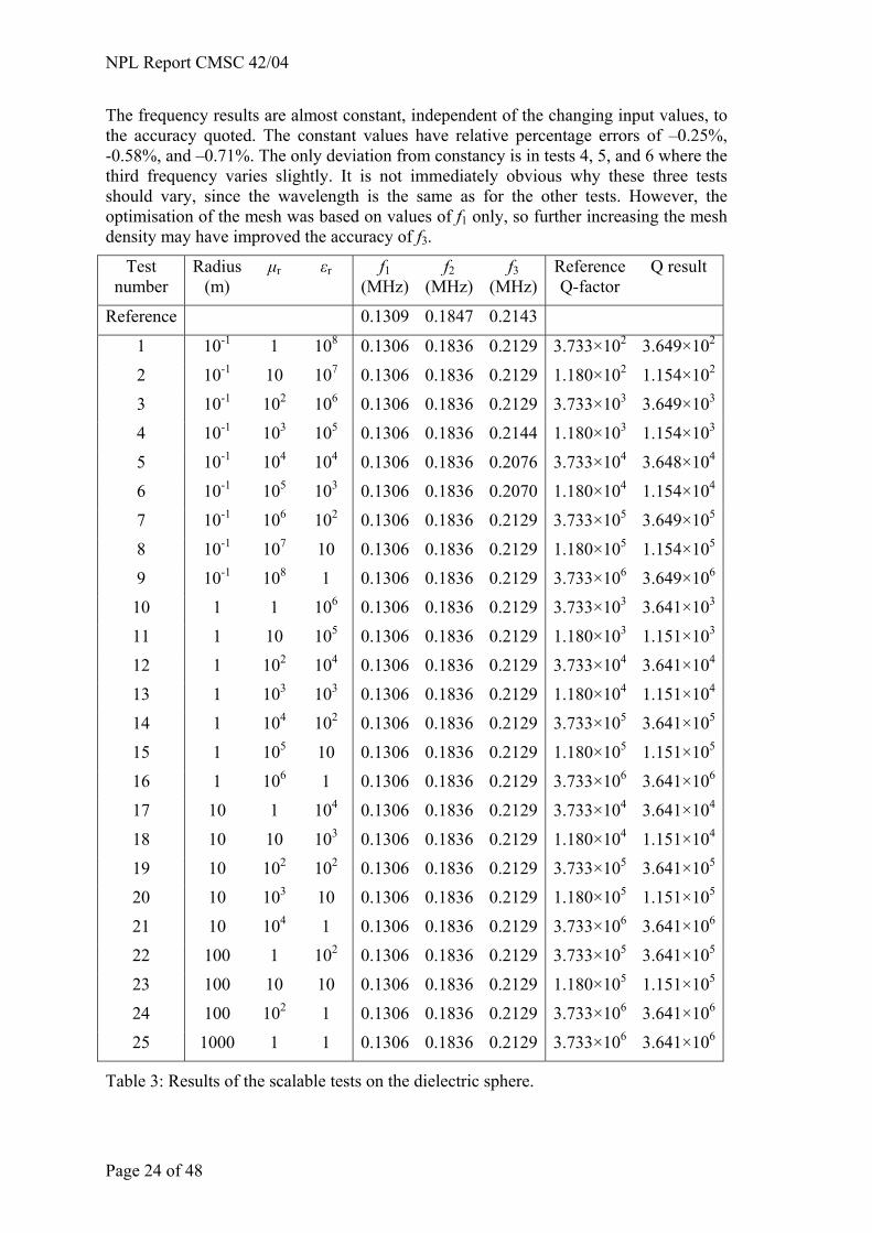
The tests that converged successfully are described in table 3. The frequency reference results are given in the first row, and the Q factor reference results are given for each test as they vary with the input values.
Page 23 of 48
NPL Report CMSC 42/04
The frequency results are almost constant, independent of the changing input values, to the accuracy quoted. The constant values have relative percentage errors of –0.25%, -0.58%, and –0.71%. The only deviation from constancy is in tests 4, 5, and 6 where the third frequency varies slightly. It is not immediately obvious why these three tests should vary, since the wavelength is the same as for the other tests. However, the optimisation of the mesh was based on values of f1 only, so further increasing the mesh density may have improved the accuracy of f3.
Test number
Radius (m)
µr εr f1 (MHz)
f2 (MHz)
f3 (MHz)
Reference Q-factor
Q result
Reference 0.1309 0.1847 0.2143
1 10-1 1 108 0.1306 0.1836 0.2129 3.733×10² 3.649×10²
2 10-1 10 107 0.1306 0.1836 0.2129 1.180×10² 1.154×10²
3 10-1 102 106 0.1306 0.1836 0.2129 3.733×10³ 3.649×10³
4 10-1 103 105 0.1306 0.1836 0.2144 1.180×10³ 1.154×10³
5 10-1 104 104 0.1306 0.1836 0.2076 3.733×10⁴ 3.648×10⁴
6 10-1 105 103 0.1306 0.1836 0.2070 1.180×10⁴ 1.154×10⁴
7 10-1 106 102 0.1306 0.1836 0.2129 3.733×10⁵ 3.649×10⁵
8 10-1 107 10 0.1306 0.1836 0.2129 1.180×10⁵ 1.154×10⁵
9 10-1 108 1 0.1306 0.1836 0.2129 3.733×10⁶ 3.649×10⁶
10 1 1 106 0.1306 0.1836 0.2129 3.733×10³ 3.641×10³
11 1 10 105 0.1306 0.1836 0.2129 1.180×10³ 1.151×10³
12 1 102 104 0.1306 0.1836 0.2129 3.733×10⁴ 3.641×10⁴
13 1 103 103 0.1306 0.1836 0.2129 1.180×10⁴ 1.151×10⁴
14 1 104 102 0.1306 0.1836 0.2129 3.733×10⁵ 3.641×10⁵
15 1 105 10 0.1306 0.1836 0.2129 1.180×10⁵ 1.151×10⁵
16 1 106 1 0.1306 0.1836 0.2129 3.733×10⁶ 3.641×10⁶
17 10 1 104 0.1306 0.1836 0.2129 3.733×10⁴ 3.641×10⁴
18 10 10 103 0.1306 0.1836 0.2129 1.180×10⁴ 1.151×10⁴
19 10 102 102 0.1306 0.1836 0.2129 3.733×10⁵ 3.641×10⁵
20 10 103 10 0.1306 0.1836 0.2129 1.180×10⁵ 1.151×10⁵
21 10 104 1 0.1306 0.1836 0.2129 3.733×10⁶ 3.641×10⁶
22 100 1 102 0.1306 0.1836 0.2129 3.733×10⁵ 3.641×10⁵
23 100 10 10 0.1306 0.1836 0.2129 1.180×10⁵ 1.151×10⁵
24 100 102 1 0.1306 0.1836 0.2129 3.733×10⁶ 3.641×10⁶
25 1000 1 1 0.1306 0.1836 0.2129 3.733×10⁶ 3.641×10⁶
Table 3: Results of the scalable tests on the dielectric sphere.
Page 24 of 48

NPL Report CMSC 42/04
Figure 14: A typical mesh of the sphere for the scalable tests. The mesh density is illustrated by the grey squares, and the coloured objects are construction points.
The results for the Q factor had relative percentage errors of between 2.2% and 2.5%. The variation in percentage relative error with trial number is shown in figure 15. The jump in values occurs when the radius of the sphere increases from 0.1 m. This may be due to the results being less converged for the smaller spheres. This lack of convergence would also explain the variation in frequency 3 results for tests 4, 5, and 6.
2.2
2.25
2.3
2.35
2.4
2.45
2.5
0 5 10 15 20 25 30
Test number
Perc
enta
ge e
rror
in th
e Q
fact
or
Figure 15: Percentage relative error in the Q factor results for the different tests.
Page 25 of 48

NPL Report CMSC 42/04
3.3.2 Coaxial sensor tests As was stated in section 3.2, the original test plan included three subsets of tests modelling coaxial sensors, based on the tests used for a previous inter-comparison exercise [14]. The software was unable to obtain converged solutions for some of these subsets.
The first subset of tests modelled a coaxial sensor and an infinite half-plane of air dielectric. The infinite half-plane was modelled as a cylinder of radius 35 mm and length 60 mm because the previous inter-comparison exercise had used this approximation. The tests converged successfully for all frequencies. The input values, reference results, and test results are shown in table 4. The test results are correct to within ± 0.1 degree, which is a much better accuracy than the repeatability of experimental measurements.
Figures 16 and 17 show typical plots of convergence behaviour for this subset of tests. Figure 16 shows the normalised change in output value versus “sweep number”. The sweep number counts the sequence of mesh refinements made by the adaptive meshing tool, and the change that is plotted is the change in value between two consecutive sweeps, labelled with the higher sweep number. Results are generally regarded as having converged when this change falls below 0.02. Figure 17 plots the number of volumes in the mesh against the sweep number. The solution for the last mesh shown on this plot took approximately 9 000 seconds (2.5 hours) to generate.
Phase angle (degrees) Phase angle (degrees) Frequency (GHz) Reference
result Test result
Frequency (GHz) Reference
result Test result
0.1 -0.38 -0.39 1.1 -4.2 -4.3
0.2 -0.77 -0.78 1.2 -4.6 -4.7
0.3 -1.15 -1.17 1.3 -5.0 -5.1
0.4 -1.5 -1.6 1.4 -5.4 -5.5
0.5 -1.9 -2 1.5 -5.8 -5.9
0.6 -2.3 -2.3 1.6 -6.2 -6.3
0.7 -2.7 -2.7 1.7 -6.6 -6.7
0.8 -3.1 -3.1 1.8 -7.0 -7.1
0.9 -3.5 -3.5 1.9 -7.4 -7.5
1.0 -3.8 -3.9 2.0 -7.8 -7.9
Table 4: Reference results and test results for the first subset of coaxial sensor model tests, modelling a coaxial sensor and an infinite half-plane of air dielectric.
Page 26 of 48

NPL Report CMSC 42/04
Figure 16: Change in output value plotted against sweep number for the air dielectric tests, showing good convergence behaviour.
Figure 17: Number of volumes in mesh plotted against sweep number.
Page 27 of 48

NPL Report CMSC 42/04
The second set of tests was unable to reach a converged solution within the time available. The first test attempted was the test with 9.97 mm of methanol, since that test was seen as most likely to converge. After five iterations of the adaptive mesh tool, the mesh consisted of around 700 000 volumes. Figure 18 shows a typical mesh for this problem. The area shaded light blue represents the bead part of the sensor. A single run of this mesh took around 22 hours to solve, and the results were still not considered to have converged. This is very poor performance compared to the 2.5 hours for a converged solution of the air model. The convergence behaviour is shown in figure 19. The minimum change in output value is approximately 0.04, which is two orders of magnitude larger than the minimum value obtained in the air tests.
The reference results for this test were an amplitude of 0.50 and a phase of –148 º. The results after five meshes were an amplitude of 0.66 and a phase of –178 º. These are clearly unsatisfactory. The reason for this poor performance is thought to be the choice of input values. As methanol allows energy to be coupled out of the probe, a resonant situation is set up with the boundaries of the problem space (which are treated as being perfect electrical conductors). The high loss of methanol damps the resonance, but not to an extent that makes the problem solvable in a reasonable amount of computing time in comparison to the first set of tests. The slow convergence is in part caused by the need to model methanol using a complex permittivity rather than a real-valued one, and significantly more computational resources are required to solve such problems.
Figure 20 shows the magnitude of the E field from one of the tests using an air dielectric. The E field is zero within the dielectric apart from an evanescent field that dies away quickly, and the reflection coefficient had a magnitude of 1.00 in all tests. Figure 21 shows the magnitude of the E field from the tests using the greatest depth of methanol dielectric. The field clearly interacts with the edge of the domain and creates a resonant effect, and the calculated reflection coefficients had magnitude less than 1.00. Although the two fields appear to decay over approximately the same distance, the scaling of the horizontal spatial dimension is misleading. Air has an electrical wavelength approximately six times that of methanol for the frequencies concerned, and for a fair comparison, the length over which the field decays should be considered in terms of number of wavelengths. Figure 22 shows a more appropriate rescaling of the methanol plot. The plot has been stretched by a scale factor of six in the horizontal direction, making the air and methanol plots more comparable, and illustrating the existence of an undamped resonance.
The third set of tests showed no signs of converging and so the results of the tests have not been reported here. As the materials to be simulated were high loss, any resonance that occurred should have been fully damped by the material, so the convergence problem is unlikely to be due to the loss factor. The poor convergence may be due to the need for modelling a complex permittivity, as mentioned above.
The good performance of the software for the tests using air dielectric shows that the algorithms that solve the time domain problems will provide accurate solutions for non-lossy materials, and will probably perform reasonably well for materials with a small imaginary part of their complex permittivity. It would be interesting to repeat these tests with a range of complex permittivities, in a non-resonant case, in order to identify how large the imaginary part of the permittivity can be before problems ensue. However, reference data for such problems are not available.
Page 28 of 48

NPL Report CMSC 42/04
Figure 18: Typical mesh for the coaxial sensor model.
Figure 19: Change in output value plotted against sweep number for the methanol dielectric tests, showing poor convergence behaviour.
Page 29 of 48

NPL Report CMSC 42/04
Figure 20: E field magnitude results for a test with air dielectric.
Figure 21: E field magnitude results for a test with methanol dielectric.
Page 30 of 48

NPL Report CMSC 42/04
Figure 22: Rescaled version of figure 21, stretched so that it is more directly comparable to figure 20.
3.4 Conclusions and extensions Two sets of problems have been run to test MWS. These problems tested the eigenvalue solver and the time domain solver over a range of input parameters.
MWS passed the majority of the eigenvalue tests, although no converged results were produced for spheres of small radius. This failure is likely to be caused by the unrealistic combination of input values.
The time domain problems using air dielectric were calculated to an accuracy better than experimental repeatability. The tests using methanol and other lossy dielectrics did not produce converged results. This may be due to the time domain algorithms being unable to simulate materials with complex permittivities accurately within a reasonable amount of computational time on the computing system used. Further tests could explore this hypothesis.
Page 31 of 48

NPL Report CMSC 42/04
4 Semiconductor dislocation modelling software Semiconductors can be created by the deposition of thin layers of material onto the surface of a much thicker substrate. The substrate and the layers are not necessarily made of the same material. If the crystal lattices of the thin layers have the same orientation as the crystal lattice of the substrate onto which they are deposited, the layers are called epitaxial layers.
Defects called dislocations can occur within the epitaxial layers. These occur where the crystal lattices of two adjacent layers do not match up precisely, commonly when one layer has an extra plane of atoms in its lattice relative to the other. The lattice mismatches caused by the dislocations produce stresses and displacements within the semiconductor.
Software has been developed to model the stresses and displacements caused by dislocations in the epitaxial layers of semiconductors. The model used is a system of fourth-order odes, and the software solves the system using an eigenvalue technique.
This software has full source code access as it was produced in-house at NPL. The central method for solution of the model, which will be outlined in section 4.2.4, is used in a slightly altered form for solution of several related problems, so the testing of this software is of benefit to several different problems.
The software is typical of a large amount of continuous modelling software, since it defines the problem of interest in physical terms instead of mathematical terms. The user does not have direct control over the coefficients of the fourth-order odes; instead the coefficients are generated when the material properties and mesh density are specified.
4.1 Details of the software 4.1.1 Physical problem A semiconductor consists of a substrate of thickness a, onto which epitaxial layers of total thickness t are deposited, where t << a. The semiconductor is regarded as infinite in one direction (the y direction), and consisting of identical units of length 2L in that direction. A typical unit is shown in figure 23. For the ease of notation, the substrate is considered as a layer throughout the following.
The use of these repeated units leads to periodic symmetry at the boundaries between units. This symmetry is useful in the mathematical formulation of this problem. It is also assumed that the system has reflective symmetry about the plane x = 0. This assumption will be true if the semiconductor has total thickness 2(a + t) and has thin films on both faces. The assumption is expected to be a good approximation for cases when t << a. It is assumed that the strain in the z direction (out of plane) is uniform and constant, so that the problem can be reduced to two dimensions.
The value of L and the origin of the axes are chosen such that the dislocations in the epitaxial layers occur in the region y = ±L, xa ≤ x ≤ xb for some values xa and xb. There may be multiple dislocations within a single semiconductor, in which case there will be sets of values xa
(i), i = 1, 2, …, n and xb(i) , i = 1, 2, …, n defining the limits of the n
dislocations.
Page 32 of 48

NPL Report CMSC 42/04
The physical problem is to predict the stress and displacement of the semiconductor due to the lattice mismatch effects. It is assumed that the semiconductor is not loaded by any external forces and the stresses are solely due to crystal lattice mismatch effects.
Substrate Epitaxial layers
a t
2L x
y
0
Figure 23: A typical periodic unit of the semiconductor. The system is assumed to be symmetric about the plane x = 0.
4.1.2 Mesh generation The first step in developing the mathematical formulation is to create a mesh. The technique used for this problem is to divide the layers into a set of strips, with the ith strip being the area xi-1 ≤ x ≤ xi, -L ≤ y ≤ L for i = 1, 2, …, N + 1. The meshing method is applied to each layer separately. The method has been chosen to produce a smooth transition between regions with different physical properties, and in particular to model the regions around the end-points of the dislocations accurately. The user has full control over the meshing, but is not provided with any visualisation of the final mesh. The final element sizes are given in one of the output files.
The meshing of each layer is defined by four numbers: the layer thickness, the number of elements n1, and the number of refinements at each end of the layer n2 and n3. Consider a layer xi-1 ≤ x ≤ xi, and let hi = xi - xi-1. The generated element sizes ej, j = 1, 2, … Ni, where Ni = n1 + n2 + n3, will be defined as follows:
Let pi = hi/n1.
For j = 1, let k = n2. Then ej = pi/2k
For j = 2, 3,...,n2 + 1, let k = n2 + 2 – j. Then ej = pi/2k.
For j = n2 + 2, …, n2 + n1 - 1, ej = pi.
For j = n2 + n1, …, n2 + n1 + n3 - 1, let k = j + 1 – (n2 + n1). Then ej = pi/2k.
Page 33 of 48

NPL Report CMSC 42/04
For j = n2 + n1 + n3, let k = n3. Then ej = pi/2k.
This produces a mesh with n1 – 2 “full sized” elements and two refined elements that are subdivided by repeatedly halving the element size. These subdivisions are used for three main reasons:
• to produce a smooth transition between substrate and coating (substrate elements are usually large because the substrate is thick and there is little variation of stress and displacement there: epitaxial layer elements are thin because the epitaxial layers are thin and the sharpest stress gradients are in the epitaxial layers),
• to provide extra detail around the ends of a dislocation since dislocations are a source of discontinuity, and a severe 1/r singularity, and
• to smooth the mesh before reaching a dislocation.
So for instance, if a laminate is made of three epitaxial layers and a substrate, and the middle layer includes a dislocation, the supplied parameters might be as follows:
Layer number Thickness (nm) n1 n2 n3
1 (Substrate) 6400 20 0 8
2 50 2 1 5
3 100 4 5 5
4 75 3 5 0
This would mean that the elements either side of all the layer boundaries were the same size (recommended practice), and that the mesh around the ends of the layer containing the dislocation (layer 3) was fine enough to capture detail. It would also mean that the element size varied from 320 nm to 0.78125 nm, which may cause computational problems.
4.1.3 Mathematical formulation The main assumptions underlying the mathematical formulation are:
• the system is in static equilibrium,
• the layers are perfectly bonded to one another,
• each layer is made from a linear orthotropic elastic material, so that its stresses and displacements are linked by twelve constants,
• the external faces of the semiconductor are stress-free,
• the stress component σyy is independent of x.
Strictly, the equations of linear orthotropic elasticity are not obeyed exactly. The assumptions required to make solution possible mean that the stress-strain equation
,TEEEy
vAzz
A
Ayy
Axx
A
a ∆+−+−=∂∂ ασνσσν 1
where v is the displacement on the y direction, νa, νA, EA, and αA are material properties, ∆T is a temperature difference and σij are the various stress components, is only obeyed in an averaged sense within each element.
These assumptions lead to a set of fourth-order differential equations of the form
Page 34 of 48

NPL Report CMSC 42/04
N,...,j,CHCGCFN
iiij
N
iiij
N
iiij 210
111
==+′′+′′′′ ∑∑∑===
(7)
where Fij, Gij, and Hij are constant coefficients generated by a set of recurrence relations, and the functions Ci, i = 1, 2, …N, are such that σxy(xi, y) = Ci’(y).
The boundary conditions applied to this system are a symmetry condition on y = 0, so that
( ) ( ) N,...,,i,CC ii 21000 ==′′′=′ , (8)
a symmetry condition on y = L, so that
( ) N,...,,i,LCi 210 ==′ , (9)
and a set of conditions, derived from considering the averaged vertical displacement of each element, that depend on whether the layer contains a dislocation:
( ) ( )[ ] ( ) ,i,LCE~h
LCLCE~h
*
A
*i
*ii
Ai1011
111
1 >=−− − layer has no dislocation (10)
( ) ( )[ ] ( ) ,i,fLCE~h
LCLCE~h
ikj
*
A
*i
*ii
Ai111
111
1 >=−− − layer has a dislocation (11)
where
( )
( ) ( )[ ] ( )[ ] ( )[ ] jk
kj
jkkj
x
xkj
i
ikj
aa,/aa
xaaxbxf
,dxxfh
fi
i
<−−−
−−−−−−=
= ∫−
22exp1
exp1exp12
11
λ
λλ (12)
It is important to note that the boundary conditions (10) and (11) are averaged across each layer. The difference between the calculated vertical displacement and the averaged value is a good measure of how well the model simulates the true physical situation. Ideally, the displacement would be uniform and constant within each element, so the closer the calculated results are to the averaged value, the better the simulation is.
The function fkj(x) is an approximation to the vertical displacement caused by a dislocation whose endpoints are x = ak and x = aj. The parameter b is the Burger’s vector of the dislocation (an indication of its direction and severity), and the parameter λ is chosen such that λ(ak - aj)/2 >> 1. In reality, the dislocation causes a discontinuity in the vertical displacement but this approach leads to a singularity in the stresses and strains which makes the problem intractable. The technique used here produces a good approximation to the discontinuity whilst allowing the stresses and strains to be calculated.
4.1.4 Solution method The solution method used for (7) has two main stages: the construction of a general solution and the calculation of the coefficients required to satisfy the boundary conditions (8), (9), (10), and (11).
The general solution is created by noting that the functions Ci are of the form
Page 35 of 48

NPL Report CMSC 42/04
( ) ( ,yByCN
jjj,ii ∑
=
=4
1
exp λ ) (13)
where the Bi,j are constants to be determined and the λj are the roots of the 4Nth order polynomial
( )( )( ) .HGFM
M
ijijijij ++=
=24
0det
λλλ
λ (14)
The polynomial (14) is a function of λ2, and so the roots of (14) must occur as pairs of positive and negative square roots. This property reduces the number of roots that need to be found to 2N. It can be shown that these 2N roots are the solutions to the generalised eigenvalue problem
,,
IF
B,I
HGA
BA
iNiii
NN
N
NN
κλκλ
κ
−==
⎥⎦
⎤⎢⎣
⎡−=⎥
⎦
⎤⎢⎣
⎡=
=
+2
00
0
xx
(15)
where the square roots are chosen to have positive real parts, 0N is the N by N zero matrix, and IN is the N by N identity matrix.
The second stage of the solution process is determination of the constants Bij. It can be shown that these constants are of the form
N,...,,i,N,...,,j,AB iN,jjj,i 21421 === −µ , (16)
where the Aj are constants that can be determined from the boundary conditions, and the µj,k can be determined from the coefficients in a factorisation of M(λj). (15) and (14) show that M(λj) = M(λj+2N), and so µj,k = µj+2N,k, j = 1, 2, …, 2N, k = 1, 2, …, N. From (8), the solution is symmetric about y = 0, and from (13) and (15) this symmetry means that Bi,j = Bi,j+2N , j = 1, 2, …, 2N, i = 1, 2, …, N and so Aj = Aj+2N , j = 1, 2, …, 2N. Hence it is only necessary to determine 2N coefficients.
These 2N coefficients are determined by substituting the expression (13) into the boundary conditions (9), (10), and (11), which results in a set of linear equations for the Ai. In order to avoid numerical overflow problems, the form (13) is slightly altered so that
( ) ( ),LyA~yCN
jjj,N-iji ∑
=
−=4
1
exp λµ
which means that the exponential term will not grow excessively large when the conditions on y = L are applied.
4.1.5 Software implementation As was mentioned in the introduction, the software was developed at NPL so the source code is fully available. The code is written in Fortran 77 and the user enters the input quantities via a text file. The software takes under a minute to perform a typical calculation on a 1.7GHz Pentium PC.
It was felt that the key step in determining the accuracy of the solution was the
Page 36 of 48

NPL Report CMSC 42/04
determination of the eigenvalues, i.e. the solution of (15). With this in mind, several versions of the software were created using different routines to carry out this calculation. The original version of the software used a public-domain routine, thought to be from a 1983 version of EISPACK [21] to calculate the eigenvalues. Two alternative versions of the software were created: one with a slightly altered version of the 1983 EISPACK routine, and one using a routine from the latest version of LAPACK. These versions are different implementations of the same algorithm, the QZ algorithm for solving generalized matrix eigenvalue problems [20, 21]. The alteration to the original routine removed an option that allowed the software to neglect very small matrix entries in order to improve stability. It was suspected that stability was being improved at the expense of accuracy.
Each version of the software was modified so that it provided the eigenvalues of maximum and minimum modulus as an output quantity as it was thought that this might be a useful indicator of the condition of the problem.
Once the different versions were prepared, they were treated as a black box, as is recommended by the testing methodology [1].
4.2 Test problem No analytical solutions have been identified for the stresses and displacements occurring in this problem in the presence of dislocations. No reference software has been found that is capable of generating reference results for the stresses and strains. This lack of reference data has led to alternative approaches being investigated for definition of test results. Three output quantities have been examined, two with a physical meaning and one that is a measure of how well the software is solving a part of the problem.
Analytical energy balance calculations [22, 23] have been carried out for semiconductors under certain restrictions. These calculations produce values for the Helmholtz free energy stored in the region between two planes of dislocations (i.e. y = ±L in figure 1). An equivalent quantity can be calculated using the software under test, and so one indication of the quality of the results is the difference between the analytical energies and those calculated using the software.
The restrictions on the semiconductor are that the substrate and epitaxial layer must have the same elastic properties, the substrate must be “infinite” (although in practice t<<a is a sufficient condition), there can only be a single epitaxial layer, and the external in-plane boundary conditions must be such that the displacements caused by the conditions are zero. These conditions can easily be simulated using the software.
As was mentioned in section 4.1.3, because the averaged boundary conditions (10) and (11) for vertical displacement are used, the maximum difference between the vertical displacement within an element and the averaged vertical displacement of that element can be used as an indication of the quality of results.
Comparison of the software results to the analytically-derived energies is not solely a test of the software: it is a test of the software, the chosen mesh, and the model validity. Similarly, the comparison between calculated and averaged displacement values is not a test of the accuracy of the software so much as it is a test of the suitability of the model. These checks are of interest to the materials scientist as they validate the model. If the quantities converge to some set of values as the mesh becomes finer, then these values will be independent of mesh and so will validate the model and the software, but it is
Page 37 of 48

NPL Report CMSC 42/04
not possible to use the result to test the software alone.
The third output quantity is the residuals obtained on substituting the calculated solution back into equation (7) and its integral with respect to y, which can be shown to be zero. This quantity is a true test of the numerical accuracy of the software as the residuals should be zero regardless of the mesh and the input quantities. It is of less interest to the materials scientist, however, and so all three quantities were investigated.
So that the analytical energy balance results could be used, the test problem was defined to fulfil the criteria outlined above. The tests had two main aims: to compare the accuracy of the solutions obtained using the different eigenvalue solvers, and to investigate the effects of varying the mesh on the results. The input parameters for the tests are shown in table 5. The material properties are those of isotropic silicon, apart from the thermal expansion coefficient which has been modified to simulate the lattice mismatch strains caused by the dislocations. An evenly spaced range of values is used for L, and the maximum value is listed in the table.
Substrate thickness (nm) 6000 Young’s modulus (GPa) 130.0
Epitaxial layer thickness (nm) 25 Poisson’s ratio
(dimensionless) 0.30
Burger’s vector (nm) [0, -0.384, 0] Thermal expansion coefficient (K-1) 1.00 × 10⁻⁵
Lattice mismatch parameter 4.2 × 10⁻³ Shear modulus (GPa) 50.0
λ as used in (E6) 5.0 L (nm) [maximum] 19.2
Table 5: Input parameters used for the test.
This problem was initially modelled using six different meshes, in order to see how the results varied with element size and distribution. The values of n1, n2, and n3 for each mesh (as explained in section 4.1.2) are given in table 6. Table 6 also shows the maximum and minimum element size within each mesh.
Substrate Epitaxial layer Mesh number n1 n2 n3 n1 n2 n3
Max size (nm)
Min size (nm)
1 20 0 2 8 2 0 200 7.8 × 10⁻¹
2 20 2 2 8 2 2 200 7.8 × 10⁻¹
3 20 0 6 8 6 0 200 4.9 × 10⁻²
4 20 0 12 8 8 0 200 1.2 × 10⁻²
5 20 0 12 8 12 0 200 7.6 × 10⁻⁴
6 20 0 20 8 20 0 200 3.0 × 10⁻⁶
Table 6: Mesh parameters and element size ranges for the meshes used in initial tests.
Page 38 of 48

NPL Report CMSC 42/04
4.3 Test results As was mentioned in section 4.2, three different output quantities have been examined. In this section, the results for each output quantity are examined in more detail.
4.3.1 Output quantity 1: Residuals of the ode systems Table 7 shows the average maximum residual of the system (7) for each mesh for the different software packages. The solution functions Ci(y) were evaluated at different values of y and substituted into (7), and the maximum residual across all values of y and all the equations was found. These calculations were repeated for 21 different values of L, and the values shown in the table are the averages of the maximum residuals. The table also shows the maximum and minimum eigenvalue moduli calculated for each mesh, which were independent of calculation method. The maximum eigenvalue modulus is not given for the final mesh because all results were thought to be unreliable for that mesh. Table 8 shows the same quantities for the system (7) integrated with respect to y.
Mesh number
Maximum eigenvalue modulus
Minimum eigenvalue modulus
Residuals: original routine
Residuals: altered routine
Residuals: new LAPACK
1 2.19 3.96 × 10⁻⁴ 1.13 × 10⁻⁴ 1.13 × 10⁻⁴ 1.32 × 10⁻⁶
2 2.21 3.96 × 10⁻⁴ 2.98 × 10⁻⁵ 2.98 × 10⁻⁵ 9.35 × 10⁻⁸
3 35.0 3.96 × 10⁻⁴ 1.77 × 10⁻⁵ 1.79 × 10⁻⁵ 8.28 × 10⁻⁶
4 134 3.96 × 10⁻⁴ 1.46 × 1061 4.71 × 10⁻⁴ 3.98 × 10⁻⁴
5 533 3.96 × 10⁻⁴ 1.00 × 10²⁰ 4.72 × 10⁻³ 1.00 × 10²⁰
6 - 3.96 × 10⁻⁴ 1.00 × 10²⁰ 3.24 × 1056 1.00 × 10²⁰
Table 7: Averaged maximum residuals of the system (7) for the six meshes for each package.
Mesh number
Maximum eigenvalue modulus
Minimum eigenvalue modulus
Residuals: original routine
Residuals: altered routine
Residuals: new LAPACK
1 2.19 3.96 × 10⁻⁴ 4.11 × 10⁻³ 4.11 × 10⁻³ 4.63 × 10⁻⁵
2 2.21 3.96 × 10⁻⁴ 1.05 × 10⁻³ 1.05 × 10⁻³ 3.44 × 10⁻⁶
3 35.0 3.96 × 10⁻⁴ 6.16 × 10⁻⁴ 6.16 × 10⁻⁴ 1.38 × 10⁻⁴
4 134 3.96 × 10⁻⁴ 1.39 × 1032 2.13 × 10⁻⁵ 8.67 × 10⁻⁶
5 533 3.96 × 10⁻⁴ 1.00 × 10²⁰ 3.78 × 10⁻⁵ 1.00 × 10²⁰
6 - 3.96 × 10⁻⁴ 1.00 × 10²⁰ 4.62 × 1034 1.00 × 10²⁰
Table 8: Averaged maximum residuals of the integral of the system (7) for the six meshes for each package.
These tables show that the original routine produces the least accurate solutions to the ode system (7), followed by the new LAPACK routine, and that the altered version of the original routine produces the best results. The tables also show that the minimum eigenvalue modulus is not affected by the increasing mesh density, which may mean that it is determined by the maximum element size (which has remained fixed
Page 39 of 48

NPL Report CMSC 42/04
throughout). Other tests, not reported here, have shown that the maximum eigenvalue modulus is approximately inversely proportional to the minimum element size.
Further investigation showed that the poor performance of the routines generally occurred when the algorithm was attempting to calculate an infinite or near-infinite eigenvalue. Infinite eigenvalues occur when the matrix B in (15) is singular, which indicates that one of the C functions includes a term that is independent of y. Since the maximum eigenvalue modulus seems to be inversely proportional to the minimum element size, there is clearly a practical limit on the minimum step size. For this set of input quantities, the extended set of results indicates that the residuals are unacceptably large (O(105)) for a minimum element size of 1.5 × 10⁻³ nm, but the residuals for a minimum element size of 3.0 × 10⁻³ nm are acceptable (O(10-3)). This estimate may depend on the material properties, and this dependence could make a good subject for further investigation.
A typical variation of maximum residual with L for the three packages is shown in figure 24. The horizontal axis is b/(2L) where b is the size of the Burger’s vector that indicates the severity of the dislocation. It is interesting to note that the most recent LAPACK routine results do not exhibit such a clear trend towards increasing with increasing b/(2L) as the other two packages.
0.00E+00
5.00E-06
1.00E-05
1.50E-05
2.00E-05
2.50E-05
3.00E-05
3.50E-05
0.00E+00 2.00E-03 4.00E-03 6.00E-03 8.00E-03 1.00E-02 1.20E-02
b/(2L)
Max
imum
resi
dual
Original routine
Altered routine
New LAPACK routine
Figure 24: Typical variation of maximum residual of the system (7) with L.
4.3.2 Output quantity 2: Free energy calculations The free energy is given by an analytic formula that holds under certain conditions. It is useful to see which, if any, of the packages agree with the analytic solution, and to examine the convergence behaviour of the free energy calculations with varying mesh. These results do not just test the software: they validate the model as well. They should be considered in conjunction with the results presented in section 4.3.1 for an overall measure of software performance.
Energy results were not available for the software using the new LAPACK routine and so only the original and altered routines were used. The original routine only produced
Page 40 of 48

NPL Report CMSC 42/04
numerical results for the first three meshes, as would be expected from the results for residuals shown in table 7. The results for these meshes were identical to those produced by the altered routine, and so only the altered routine results will be discussed.
The altered routine produced results for all six of the original meshes, despite the large residual results produced using the sixth mesh. This is somewhat surprising, and an explanation has not been identified yet. Energy results were produced for a series of meshes defined in table 9. These meshes were designed to have elements of the same size on either side of the interface between the substrate and the epitaxial layer. The analytic solution is given in terms of b/(2L), and the analytic solution and two calculated solutions are plotted against b/(2L) in figure 25.
Substrate Epitaxial layer Mesh number n1 n2 n3 n1 n2 n3
Max size (nm)
Min size (nm)
7 20 0 6 8 0 0 200 3.1
8 20 0 8 8 2 0 200 7.8 × 10⁻¹
9 20 0 10 8 4 0 200 2.0 × 10⁻¹
10 20 0 12 8 6 0 200 4.9 × 10⁻²
11 20 0 16 8 10 0 200 3.1 × 10⁻³
12 20 0 20 8 14 0 200 1.9 × 10⁻⁴
Table 9: Additional meshes used for energy calculations.
-0.06
-0.04
-0.02
0
0.02
0.04
0.06
0 0.002 0.004 0.006 0.008 0.01 0.012
b/(2L)
Ener
gy (J
)
Analytic solutionMesh 1Mesh 12
Figure 25: Analytic energy solution for an infinite array of dislocations and two solutions calculated by the altered version of the software using meshes 1 and 12.
Table 10 gives the root mean square difference, summed over 21 values of b/(2L),
Page 41 of 48

NPL Report CMSC 42/04
between the analytic and calculated solutions for each mesh. The table also shows the minimum element size for each mesh, and the corresponding average maximum residual of the odes calculated by the altered version of the software.
Mesh number RMS difference (J) Minimum element size (nm)
Average max ode residuals
1 3.6 × 10-27.8 × 10-1 1.13 × 10⁻⁴
2 3.6 × 10-27.8 × 10-1 2.98 × 10⁻⁵
3 7.2 × 10-34.9 × 10-2 1.79 × 10⁻⁵
4 1.3 × 10-41.2 × 10-2 4.71 × 10⁻⁴
5 1.4 × 10-47.6 × 10-4 4.72 × 10⁻³
6 5.4 × 10-43.0 × 10-6 3.24 × 1056
7 1.4 × 10-23.1 2.01 × 10⁻⁴
8 6.0 × 10-37.8 × 10-1 2.42 × 10⁻⁵
9 1.3 × 10-32.0 × 10-1 1.78 × 10⁻⁵
10 5.9 × 10-54.9 × 10-2 5.81 × 10⁻⁵
11 1.6 × 10-43.1 × 10-3 6.41 × 10⁻³
12 1.7 × 10-41.9 × 10-4 9.35 × 10⁹
Table 10: RMS differences between the analytic expression for the free energy and the calculated solutions.
Whilst there are no clear-cut trends in table 10, some broad conclusions can be drawn. The first is that the calculated energy values appear to converge to the analytic solution for the energy as the minimum element size decreases. This property is important because it validates the model against an independent solution. The property is probably caused by the increasing number of elements rather than the decreasing minimum size, although no further investigation has been carried out to check this.
The second broad conclusion is that the software has produced a good result for the free energy despite the overall solution being of poor quality (demonstrated by the large average residual). This is not a good property, since the good energy result could mislead the user as to the overall quality of their results. This behaviour illustrates the dangers of testing software or validating a model against a single property of a complicated system, such as energy or mass: a solution with incorrect detailed results can still produce the correct overall property, leading to false acceptance of a poor model.
Page 42 of 48
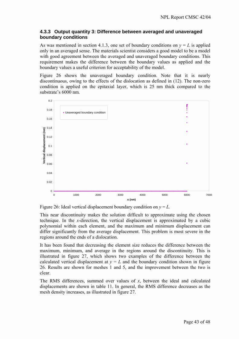
NPL Report CMSC 42/04
4.3.3 Output quantity 3: Difference between averaged and unaveraged boundary conditions As was mentioned in section 4.1.3, one set of boundary conditions on y = L is applied only in an averaged sense. The materials scientist considers a good model to be a model with good agreement between the averaged and unaveraged boundary conditions. This requirement makes the difference between the boundary values as applied and the boundary values a useful criterion for acceptability of the model.
Figure 26 shows the unaveraged boundary condition. Note that it is nearly discontinuous, owing to the effects of the dislocation as defined in (12). The non-zero condition is applied on the epitaxial layer, which is 25 nm thick compared to the substrate’s 6000 nm.
0
0.02
0.04
0.06
0.08
0.1
0.12
0.14
0.16
0.18
0.2
0 1000 2000 3000 4000 5000 6000 7000
x (nm)
Ver
tical
dis
plac
emen
t (nm
)
Unaveraged boundary condition
Figure 26: Ideal vertical displacement boundary condition on y = L.
This near discontinuity makes the solution difficult to approximate using the chosen technique. In the x-direction, the vertical displacement is approximated by a cubic polynomial within each element, and the maximum and minimum displacement can differ significantly from the average displacement. This problem is most severe in the regions around the ends of a dislocation.
It has been found that decreasing the element size reduces the difference between the maximum, minimum, and average in the regions around the discontinuity. This is illustrated in figure 27, which shows two examples of the difference between the calculated vertical displacement at y = L and the boundary condition shown in figure 26. Results are shown for meshes 1 and 5, and the improvement between the two is clear.
The RMS differences, summed over values of x, between the ideal and calculated displacements are shown in table 11. In general, the RMS difference decreases as the mesh density increases, as illustrated in figure 27.
Page 43 of 48

NPL Report CMSC 42/04
Mesh No. 1 2 3 4 5 6
RMS difference
5.78 × 10⁻² 5.53 × 10⁻² 6.68 × 10⁻² 5.77 × 10⁻⁴ 2.09 × 10⁻³ 4.28 × 10¹³
Mesh No. 7 8 9 10 11 12
RMS difference
1.25 × 10⁻² 9.38 × 10⁻³ 3.85 × 10⁻³ 1.09 × 10⁻³ 9.12 × 10⁻⁵ 8.06 × 10⁴
Table 11: RMS differences between the ideal and calculated vertical boundary displacements for the meshes.
-0.3
-0.2
-0.1
0
0.1
0.2
0.3
0 1000 2000 3000 4000 5000 6000 7000
x (nm)
Idea
l bou
ndar
y di
spla
cem
ent -
Cal
cula
ted
boun
dary
dis
plac
emen
t (n
m) Mesh 1
Mesh 5
Figure 27: Difference between ideal vertical boundary displacement and calculated vertical boundary displacement for meshes 1 and 5.
4.4 Conclusions and extensions Testing has been carried out on three different versions of a software package that models dislocations in semiconductors by solving a system of fourth-order odes. The aim of the testing was to investigate which of the packages produced accurate results for a wide range of mesh parameters, since the mesh affects how close the calculated solution is to the ideal solution.
The continuous modelling software testing methodology could not be applied due to a lack of analytic solutions making the identification of reference results difficult. Instead, three other criteria have been used for assessing the performance of the packages. The main criterion is the maximum size of the residuals obtained by substituting the calculated solution back into the odes.
The testing has shown that the original version of the software produces accurate solutions with small residuals over a smaller range of mesh parameters than the other two versions of the software. One of the other versions is suspected to have stability problems since the alteration that was made to produce the software was expected to lead to accumulation of errors, but this has not shown up in the test results. The third
Page 44 of 48

NPL Report CMSC 42/04
version of the software is expected to be reliable, stable, and accurate since it is based on an LAPACK routine.
The routine for solution of the eigenvalue problem can produce the eigenvectors as part of the solution procedure. At the moment, the software uses the eigenvalues but does not consider any potential uses of the eigenvectors. If the eigenvectors were calculated, they could provide an estimate of the condition number of the problem, which could be a useful guide as to the likely accuracy of the results. Additionally, it may be possible to use the eigenvectors during the calculation involving the boundary conditions.
This case study has illustrated the difficulty of testing software that solves problems for which reference solutions are not available. The study has also shown that combining testing with validation can reach an end result that is of more use to the end user than testing alone.
Page 45 of 48

NPL Report CMSC 42/04
5 Conclusions This report has demonstrated the advice given on testing continuous modelling software in the companion report to this one [1] by applying the techniques described there to three case studies.
The first case study tested software implementations of the boundary element method for simulation of propagation and scattering of acoustic waves. One software package was used as reference software, because it was shown to produce results identical to a given accuracy using two independent mathematical methods. Two test problems were used to investigate two software packages. One problem was expected to be straightforward to solve, and the other was designed to test the most important aspect of the packages. The test results showed that both of the packages produced accurate results for both problems. The study showed that where reference software is available it can be a very useful source of reference results. Further investigations into the parameters affecting the test results are planned.
The second case study applied two sets of test problems to a computational electromagnetic software package. One set of tests was a scalable set, as recommended in the methodology for testing continuous modelling software. The other set had been used in a previous software intercomparison exercise, which had used several independent calculation methods to produce the same results. Some of the test problems did not produce converged results within an acceptable time. It is thought that these problems are outside of the capabilities of the package under test, and further investigations exploring the limits of the software’s capabilities may take place in future.
The third case study tested software that solved a system of fourth order differential equations to simulate the displacements, stresses and strains in a semiconductor containing dislocations. Three quantities were used as test results: two that were physically important quantities that gave an insight into how well the model described the physical system, and one that measured the mathematical accuracy of the solution to the system of differential equations. In effect, the physical quantities were being used for model validation and the software test result was the mathematical accuracy of the solution. The results showed that the physical quantities could not always identify a mathematically inaccurate solution, and provided useful information about how to obtain an accurate solution by choosing input parameters carefully.
The work described has illustrated several of the common difficulties involved in testing continuous modelling software, in particular
• the difficulty of obtaining reference solutions,
• the difficulty of defining the capabilities of a package precisely before use,
• the question of whether to define a mesh for the test problem or to use automatic meshing tools, and
• the hazards of using global quantities, such as energy, as test results.
The work also showed the benefits of testing software thoroughly, the use of scalable tests in investigating how software accuracy varies with input parameters, and how combining testing with validation can achieve an end result that is of more use to the end user than testing alone.
Page 46 of 48
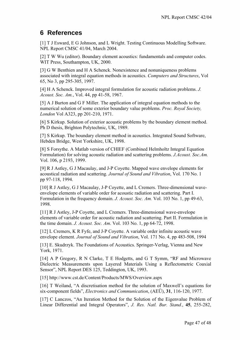
NPL Report CMSC 42/04
6 References [1] T J Esward, E G Johnson, and L Wright. Testing Continuous Modelling Software. NPL Report CMSC 41/04, March 2004.
[2] T W Wu (editor). Boundary element acoustics: fundamentals and computer codes. WIT Press, Southampton, UK, 2000.
[3] G W Benthien and H A Schenck. Nonexistence and nonuniqueness problems associated with integral equation methods in acoustics. Computers and Structures, Vol 65, No 3, pp 295-305, 1997.
[4] H A Schenck. Improved integral formulation for acoustic radiation problems. J. Acoust. Soc. Am., Vol. 44, pp 41-58, 1967.
[5] A J Burton and G F Miller. The application of integral equation methods to the numerical solution of some exterior boundary value problems. Proc. Royal Society, London Vol A323, pp 201-210, 1971.
[6] S Kirkup. Solution of exterior acoustic problems by the boundary element method. Ph D thesis, Brighton Polytechnic, UK, 1989.
[7] S Kirkup. The boundary element method in acoustics. Integrated Sound Software, Hebden Bridge, West Yorkshire, UK, 1998.
[8] S Forsythe. A Matlab version of CHIEF (Combined Helmholtz Integral Equation Formulation) for solving acoustic radiation and scattering problems. J.Acoust. Soc.Am. Vol. 106, p 2193, 1999.
[9] R J Astley, G J Macaulay, and J-P Coyette. Mapped wave envelope elements for acoustical radiation and scattering. Journal of Sound and Vibration, Vol. 170 No. 1 pp 97-118, 1994.
[10] R J Astley, G J Macaulay, J-P Coyette, and L Cremers. Three-dimensional wave-envelope elements of variable order for acoustic radiation and scattering. Part I. Formulation in the frequency domain. J. Acoust. Soc. Am. Vol. 103 No. 1, pp 49-63, 1998.
[11] R J Astley, J-P Coyette, and L Cremers. Three-dimensional wave-envelope elements of variable order for acoustic radiation and scattering. Part II. Formulation in the time domain. J. Acoust. Soc. Am. Vol. 103 No. 1, pp 64-72, 1998.
[12] L Cremers, K R Fyfe, and J-P Coyette. A variable order infinite acoustic wave envelope element. Journal of Sound and Vibration, Vol. 171 No. 4, pp 483-508, 1994
[13] E. Skudrzyk. The Foundations of Acoustics. Springer-Verlag, Vienna and New York, 1971.
[14] A P Gregory, R N Clarke, T E Hodgetts, and G T Symm, “RF and Microwave Dielectric Measurements upon Layered Materials Using a Reflectometric Coaxial Sensor”, NPL Report DES 125, Teddington, UK, 1993.
[15] http://www.cst.de/Content/Products/MWS/Overview.aspx
[16] T Weiland, “A discretisation method for the solution of Maxwell’s equations for six-component fields”, Electronics and Communication, (AEÜ), 31, 116-120, 1977.
[17] C Lanczos, “An Iteration Method for the Solution of the Eigenvalue Problem of Linear Differential and Integral Operators”, J. Res. Natl. Bur. Stand., 45, 255-282,
Page 47 of 48

NPL Report CMSC 42/04
1950.
[18] B Krietenstein, R Schuhmann, P Thoma and T Weiland, “The Perfect Boundary Approximation technique facing the challenge of high precision field computation”, Proc. XIX International Linear Accerlerator Conference (LINAC ’98), Chicago, USA. 860-862, 1998.
[19] C A Balanis, “Advanced Engineering Electromagnetics”, John Wiley & Sons ISBN 0-471-62194-3, 1989.
[20] C B Moler and G W Stewart. An algorithm for the generalized eigenvalue problem. SIAM J. Numer. Anal., 10, 241-256, 1973.
[21] http://www.netlib.org/lapack/
[22] J R Willis, S C Jain and R Bullough. The strain energy of an array of dislocations: implications for strain relaxation in semiconductor heterostructures. Phil. Mag., 62, 115-129, 1990.
[23] T J Gosling, S C Jain, J R Willis, A Atkinson and R Bullough. Stable configurations in strained epitaxial layers. Phil. Mag., 66, 119-132, 1992.
Page 48 of 48